Embed Size (px)
Citation preview
Lecture Notes in:
FRACTURE MECHANICS
Victor E. SaoumaDept. of Civil Environmental and Architectural Engineering
University of Colorado, Boulder, CO 80309-0428

ii
Victor Saouma Fracture Mechanics

Contents
I INTRODUCTION 3
1 INTRODUCTION 51.1 Modes of Failures . . . . . . . . . . . . . . . . . . . . . . . . . . . . . . . . . . . . 51.2 Examples of Structural Failures Caused by Fracture . . . . . . . . . . . . . . . . 61.3 Fracture Mechanics vs Strength of Materials . . . . . . . . . . . . . . . . . . . . . 71.4 Major Historical Developments in Fracture Mechanics . . . . . . . . . . . . . . . 111.5 Coverage . . . . . . . . . . . . . . . . . . . . . . . . . . . . . . . . . . . . . . . . . 13
2 PRELIMINARY CONSIDERATIONS 152.1 Tensors . . . . . . . . . . . . . . . . . . . . . . . . . . . . . . . . . . . . . . . . . 15
2.1.1 Indicial Notation . . . . . . . . . . . . . . . . . . . . . . . . . . . . . . . . 162.1.2 Tensor Operations . . . . . . . . . . . . . . . . . . . . . . . . . . . . . . . 182.1.3 Rotation of Axes . . . . . . . . . . . . . . . . . . . . . . . . . . . . . . . . 182.1.4 Trace . . . . . . . . . . . . . . . . . . . . . . . . . . . . . . . . . . . . . . 192.1.5 Inverse Tensor . . . . . . . . . . . . . . . . . . . . . . . . . . . . . . . . . 202.1.6 Principal Values and Directions of Symmetric Second Order Tensors . . . 20
2.2 Kinetics . . . . . . . . . . . . . . . . . . . . . . . . . . . . . . . . . . . . . . . . . 212.2.1 Force, Traction and Stress Vectors . . . . . . . . . . . . . . . . . . . . . . 212.2.2 Traction on an Arbitrary Plane; Cauchy’s Stress Tensor . . . . . . . . . . 22E 2-1 Stress Vectors . . . . . . . . . . . . . . . . . . . . . . . . . . . . . . . . . . 242.2.3 Invariants . . . . . . . . . . . . . . . . . . . . . . . . . . . . . . . . . . . . 242.2.4 Spherical and Deviatoric Stress Tensors . . . . . . . . . . . . . . . . . . . 252.2.5 Stress Transformation . . . . . . . . . . . . . . . . . . . . . . . . . . . . . 252.2.6 Polar Coordinates . . . . . . . . . . . . . . . . . . . . . . . . . . . . . . . 26
2.3 Kinematic . . . . . . . . . . . . . . . . . . . . . . . . . . . . . . . . . . . . . . . . 262.3.1 Strain Tensors . . . . . . . . . . . . . . . . . . . . . . . . . . . . . . . . . 262.3.2 Compatibility Equation . . . . . . . . . . . . . . . . . . . . . . . . . . . . 29
2.4 Fundamental Laws of Continuum Mechanics . . . . . . . . . . . . . . . . . . . . . 292.4.1 Conservation Laws . . . . . . . . . . . . . . . . . . . . . . . . . . . . . . . 302.4.2 Fluxes . . . . . . . . . . . . . . . . . . . . . . . . . . . . . . . . . . . . . . 302.4.3 Conservation of Mass; Continuity Equation . . . . . . . . . . . . . . . . . 312.4.4 Linear Momentum Principle; Equation of Motion . . . . . . . . . . . . . . 32

iv CONTENTS
2.4.5 Moment of Momentum Principle . . . . . . . . . . . . . . . . . . . . . . . 332.4.6 Conservation of Energy; First Principle of Thermodynamics . . . . . . . . 33
2.5 Constitutive Equations . . . . . . . . . . . . . . . . . . . . . . . . . . . . . . . . . 342.5.1 Transversly Isotropic Case . . . . . . . . . . . . . . . . . . . . . . . . . . . 362.5.2 Special 2D Cases . . . . . . . . . . . . . . . . . . . . . . . . . . . . . . . . 36
2.5.2.1 Plane Strain . . . . . . . . . . . . . . . . . . . . . . . . . . . . . 362.5.2.2 Axisymmetry . . . . . . . . . . . . . . . . . . . . . . . . . . . . . 362.5.2.3 Plane Stress . . . . . . . . . . . . . . . . . . . . . . . . . . . . . 37
2.6 Airy Stress Function . . . . . . . . . . . . . . . . . . . . . . . . . . . . . . . . . . 372.7 Complex Variables . . . . . . . . . . . . . . . . . . . . . . . . . . . . . . . . . . . 38
2.7.1 Complex Airy Stress Functions . . . . . . . . . . . . . . . . . . . . . . . . 392.8 Curvilinear Coordinates . . . . . . . . . . . . . . . . . . . . . . . . . . . . . . . . 402.9 Basic Equations of Anisotropic Elasticity . . . . . . . . . . . . . . . . . . . . . . 42
2.9.1 Coordinate Transformations . . . . . . . . . . . . . . . . . . . . . . . . . . 442.9.2 Plane Stress-Strain Compliance Transformation . . . . . . . . . . . . . . . 442.9.3 Stress Functions . . . . . . . . . . . . . . . . . . . . . . . . . . . . . . . . 452.9.4 Stresses and Displacements . . . . . . . . . . . . . . . . . . . . . . . . . . 47
2.10 Conclusion . . . . . . . . . . . . . . . . . . . . . . . . . . . . . . . . . . . . . . . 48
II LINEAR ELASTIC FRACTURE MECHANICS 49
3 ELASTICITY BASED SOLUTIONS FOR CRACK PROBLEMS 513.1 Introduction . . . . . . . . . . . . . . . . . . . . . . . . . . . . . . . . . . . . . . . 513.2 Circular Hole, (Kirsch, 1898) . . . . . . . . . . . . . . . . . . . . . . . . . . . . . 513.3 Elliptical hole in a Uniformly Stressed Plate (Inglis, 1913) . . . . . . . . . . . . . 553.4 Crack, (Westergaard, 1939) . . . . . . . . . . . . . . . . . . . . . . . . . . . . . . 57
3.4.1 Stress Intensity Factors (Irwin) . . . . . . . . . . . . . . . . . . . . . . . . 623.4.2 Near Crack Tip Stresses and Displacements in Isotropic Cracked Solids . 64
3.5 V Notch, (Williams, 1952) . . . . . . . . . . . . . . . . . . . . . . . . . . . . . . . 653.6 Crack at an Interface between Two Dissimilar Materials (Williams, 1959) . . . . 70
3.6.1 General Function . . . . . . . . . . . . . . . . . . . . . . . . . . . . . . . . 703.6.2 Boundary Conditions . . . . . . . . . . . . . . . . . . . . . . . . . . . . . 703.6.3 Homogeneous Equations . . . . . . . . . . . . . . . . . . . . . . . . . . . . 723.6.4 Solve for λ . . . . . . . . . . . . . . . . . . . . . . . . . . . . . . . . . . . 733.6.5 Near Crack Tip Stresses . . . . . . . . . . . . . . . . . . . . . . . . . . . . 74
3.7 Homogeneous Anisotropic Material (Sih and Paris) . . . . . . . . . . . . . . . . . 773.8 Assignment . . . . . . . . . . . . . . . . . . . . . . . . . . . . . . . . . . . . . . . 79
4 LEFM DESIGN EXAMPLES 834.1 Design Philosophy Based on Linear Elastic Fracture Mechanics . . . . . . . . . . 834.2 Stress Intensity Factors . . . . . . . . . . . . . . . . . . . . . . . . . . . . . . . . 844.3 Fracture Properties of Materials . . . . . . . . . . . . . . . . . . . . . . . . . . . . 94
Victor Saouma Fracture Mechanics

CONTENTS v
4.4 Examples . . . . . . . . . . . . . . . . . . . . . . . . . . . . . . . . . . . . . . . . 954.4.1 Example 1 . . . . . . . . . . . . . . . . . . . . . . . . . . . . . . . . . . . . 954.4.2 Example 2 . . . . . . . . . . . . . . . . . . . . . . . . . . . . . . . . . . . . 96
4.5 Additional Design Considerations . . . . . . . . . . . . . . . . . . . . . . . . . . . 974.5.1 Leak Before Fail . . . . . . . . . . . . . . . . . . . . . . . . . . . . . . . . 974.5.2 Damage Tolerance Assessment . . . . . . . . . . . . . . . . . . . . . . . . 98
5 THEORETICAL STRENGTH of SOLIDS; (Griffith I) 995.1 Derivation . . . . . . . . . . . . . . . . . . . . . . . . . . . . . . . . . . . . . . . . 99
5.1.1 Tensile Strength . . . . . . . . . . . . . . . . . . . . . . . . . . . . . . . . 1005.1.1.1 Ideal Strength in Terms of Physical Parameters . . . . . . . . . 1005.1.1.2 Ideal Strength in Terms of Engineering Parameter . . . . . . . . 103
5.1.2 Shear Strength . . . . . . . . . . . . . . . . . . . . . . . . . . . . . . . . . 1035.2 Griffith Theory . . . . . . . . . . . . . . . . . . . . . . . . . . . . . . . . . . . . . 104
5.2.1 Derivation . . . . . . . . . . . . . . . . . . . . . . . . . . . . . . . . . . . . 104
6 ENERGY TRANSFER in CRACK GROWTH; (Griffith II) 1076.1 Thermodynamics of Crack Growth . . . . . . . . . . . . . . . . . . . . . . . . . . 108
6.1.1 General Derivation . . . . . . . . . . . . . . . . . . . . . . . . . . . . . . . 1086.1.2 Brittle Material, Griffith’s Model . . . . . . . . . . . . . . . . . . . . . . . 109
6.2 Energy Release Rate; Global . . . . . . . . . . . . . . . . . . . . . . . . . . . . . 1126.2.1 From Load-Displacement . . . . . . . . . . . . . . . . . . . . . . . . . . . 1126.2.2 From Compliance . . . . . . . . . . . . . . . . . . . . . . . . . . . . . . . . 113
6.3 Energy Release Rate; Local . . . . . . . . . . . . . . . . . . . . . . . . . . . . . . 1156.4 Crack Stability . . . . . . . . . . . . . . . . . . . . . . . . . . . . . . . . . . . . . 117
6.4.1 Effect of Geometry; Π Curve . . . . . . . . . . . . . . . . . . . . . . . . . 1176.4.2 Effect of Material; R Curve . . . . . . . . . . . . . . . . . . . . . . . . . . 118
6.4.2.1 Theoretical Basis . . . . . . . . . . . . . . . . . . . . . . . . . . . 1196.4.2.2 R vs KIc . . . . . . . . . . . . . . . . . . . . . . . . . . . . . . . 1196.4.2.3 Plane Strain . . . . . . . . . . . . . . . . . . . . . . . . . . . . . 1206.4.2.4 Plane Stress . . . . . . . . . . . . . . . . . . . . . . . . . . . . . 122
7 MIXED MODE CRACK PROPAGATION 1257.1 Analytical Models for Isotropic Solids . . . . . . . . . . . . . . . . . . . . . . . . 126
7.1.1 Maximum Circumferential Tensile Stress. . . . . . . . . . . . . . . . . . . 1267.1.2 Maximum Energy Release Rate . . . . . . . . . . . . . . . . . . . . . . . . 1277.1.3 Minimum Strain Energy Density Criteria. . . . . . . . . . . . . . . . . . . 1297.1.4 Observations . . . . . . . . . . . . . . . . . . . . . . . . . . . . . . . . . . 131
7.2 Empirical Models for Rocks . . . . . . . . . . . . . . . . . . . . . . . . . . . . . . 1337.3 Extensions to Anisotropic Solids . . . . . . . . . . . . . . . . . . . . . . . . . . . 1347.4 Interface Cracks . . . . . . . . . . . . . . . . . . . . . . . . . . . . . . . . . . . . 140
7.4.1 Crack Tip Fields . . . . . . . . . . . . . . . . . . . . . . . . . . . . . . . . 1407.4.2 Dimensions of Bimaterial Stress Intensity Factors . . . . . . . . . . . . . . 142
Victor Saouma Fracture Mechanics

vi CONTENTS
7.4.3 Interface Fracture Toughness . . . . . . . . . . . . . . . . . . . . . . . . . 1437.4.3.1 Interface Fracture Toughness when β = 0 . . . . . . . . . . . . . 1457.4.3.2 Interface Fracture Toughness when β �= 0 . . . . . . . . . . . . . 146
7.4.4 Crack Kinking Analysis . . . . . . . . . . . . . . . . . . . . . . . . . . . . 1477.4.4.1 Numerical Results from He and Hutchinson . . . . . . . . . . . 1477.4.4.2 Numerical Results Using Merlin . . . . . . . . . . . . . . . . . . 149
7.4.5 Summary . . . . . . . . . . . . . . . . . . . . . . . . . . . . . . . . . . . . 154
III ELASTO PLASTIC FRACTURE MECHANICS 157
8 PLASTIC ZONE SIZES 1598.1 Uniaxial Stress Criteria . . . . . . . . . . . . . . . . . . . . . . . . . . . . . . . . 160
8.1.1 First-Order Approximation. . . . . . . . . . . . . . . . . . . . . . . . . . . 1608.1.2 Second-Order Approximation (Irwin) . . . . . . . . . . . . . . . . . . . . . 160
8.1.2.1 Example . . . . . . . . . . . . . . . . . . . . . . . . . . . . . . . 1628.1.3 Dugdale’s Model. . . . . . . . . . . . . . . . . . . . . . . . . . . . . . . . . 163
8.2 Multiaxial Yield Criteria . . . . . . . . . . . . . . . . . . . . . . . . . . . . . . . . 1658.3 Plane Strain vs. Plane Stress . . . . . . . . . . . . . . . . . . . . . . . . . . . . . 168
9 FATIGUE CRACK PROPAGATION 1719.1 Experimental Observation . . . . . . . . . . . . . . . . . . . . . . . . . . . . . . . 1729.2 Fatigue Laws Under Constant Amplitude Loading . . . . . . . . . . . . . . . . . 172
9.2.1 Paris Model . . . . . . . . . . . . . . . . . . . . . . . . . . . . . . . . . . . 1739.2.2 Foreman’s Model . . . . . . . . . . . . . . . . . . . . . . . . . . . . . . . . 1749.2.3 Modified Walker’s Model . . . . . . . . . . . . . . . . . . . . . . . . . . . 1749.2.4 Table Look-Up . . . . . . . . . . . . . . . . . . . . . . . . . . . . . . . . . 1749.2.5 Effective Stress Intensity Factor Range . . . . . . . . . . . . . . . . . . . 1759.2.6 Examples . . . . . . . . . . . . . . . . . . . . . . . . . . . . . . . . . . . . 175
9.2.6.1 Example 1 . . . . . . . . . . . . . . . . . . . . . . . . . . . . . . 1759.2.6.2 Example 2 . . . . . . . . . . . . . . . . . . . . . . . . . . . . . . 1769.2.6.3 Example 3 . . . . . . . . . . . . . . . . . . . . . . . . . . . . . . 176
9.3 Variable Amplitude Loading . . . . . . . . . . . . . . . . . . . . . . . . . . . . . . 1769.3.1 No Load Interaction . . . . . . . . . . . . . . . . . . . . . . . . . . . . . . 1769.3.2 Load Interaction . . . . . . . . . . . . . . . . . . . . . . . . . . . . . . . . 177
9.3.2.1 Observation . . . . . . . . . . . . . . . . . . . . . . . . . . . . . 1779.3.2.2 Retardation Models . . . . . . . . . . . . . . . . . . . . . . . . . 177
9.3.2.2.1 Wheeler’s Model . . . . . . . . . . . . . . . . . . . . . . 1789.3.2.2.2 Generalized Willenborg’s Model . . . . . . . . . . . . . 178
Victor Saouma Fracture Mechanics
CONTENTS vii
10 CRACK TIP OPENING DISPLACEMENTS 18110.1 Derivation of CTOD . . . . . . . . . . . . . . . . . . . . . . . . . . . . . . . . . . 182
10.1.1 Irwin’s Solution . . . . . . . . . . . . . . . . . . . . . . . . . . . . . . . . . 18210.1.2 Dugdale’s Solution . . . . . . . . . . . . . . . . . . . . . . . . . . . . . . . 183
10.2 G-CTOD Relations . . . . . . . . . . . . . . . . . . . . . . . . . . . . . . . . . . . 184
11 J INTEGRAL 18511.1 Genesis . . . . . . . . . . . . . . . . . . . . . . . . . . . . . . . . . . . . . . . . . 18511.2 Proof of Path Independence . . . . . . . . . . . . . . . . . . . . . . . . . . . . . . 18611.3 Nonlinear Elastic Energy Release Rate . . . . . . . . . . . . . . . . . . . . . . . . 187
11.3.1 Virtual Line Crack Extension . . . . . . . . . . . . . . . . . . . . . . . . . 18811.3.2 †Virtual Volume Expansion . . . . . . . . . . . . . . . . . . . . . . . . . . 189
11.4 Nonlinear Energy Release Rate . . . . . . . . . . . . . . . . . . . . . . . . . . . . 19211.5 J Testing . . . . . . . . . . . . . . . . . . . . . . . . . . . . . . . . . . . . . . . . 19411.6 Crack Growth Resistance Curves . . . . . . . . . . . . . . . . . . . . . . . . . . . 19411.7 † Load Control versus Displacement Control . . . . . . . . . . . . . . . . . . . . . 19611.8 Plastic Crack Tip Fields . . . . . . . . . . . . . . . . . . . . . . . . . . . . . . . . 19711.9 Engineering Approach to Fracture . . . . . . . . . . . . . . . . . . . . . . . . . . 202
11.9.1 Compilation of Fully Plastic Solutions . . . . . . . . . . . . . . . . . . . . 20411.9.2 Numerical Example . . . . . . . . . . . . . . . . . . . . . . . . . . . . . . 215
11.10J1 and J2 Generalization. . . . . . . . . . . . . . . . . . . . . . . . . . . . . . . . 21611.11Dynamic Energy Release Rate . . . . . . . . . . . . . . . . . . . . . . . . . . . . 21711.12Effect of Other Loading . . . . . . . . . . . . . . . . . . . . . . . . . . . . . . . . 219
11.12.1 Surface Tractions on Crack Surfaces . . . . . . . . . . . . . . . . . . . . . 21911.12.2 Body Forces . . . . . . . . . . . . . . . . . . . . . . . . . . . . . . . . . . . 22011.12.3 Initial Strains Corresponding to Thermal Loading . . . . . . . . . . . . . 22011.12.4 Initial Stresses Corresponding to Pore Pressures . . . . . . . . . . . . . . 22311.12.5 Combined Thermal Strains and Pore Pressures . . . . . . . . . . . . . . . 225
11.13Epilogue . . . . . . . . . . . . . . . . . . . . . . . . . . . . . . . . . . . . . . . . . 226
IV FRACTURE MECHANICS OF CONCRETE 227
12 FRACTURE DETERIORATION ANALYSIS OF CONCRETE 22912.1 Introduction . . . . . . . . . . . . . . . . . . . . . . . . . . . . . . . . . . . . . . . 22912.2 Phenomenological Observations . . . . . . . . . . . . . . . . . . . . . . . . . . . . 230
12.2.1 Load, Displacement, and Strain Control Tests . . . . . . . . . . . . . . . . 23012.2.2 Pre/Post-Peak Material Response of Steel and Concrete . . . . . . . . . . 231
12.3 Localisation of Deformation . . . . . . . . . . . . . . . . . . . . . . . . . . . . . . 23212.3.1 Experimental Evidence . . . . . . . . . . . . . . . . . . . . . . . . . . . . 232
12.3.1.1 σ-COD Diagram, Hillerborg’s Model . . . . . . . . . . . . . . . . 23312.3.2 Theoretical Evidence . . . . . . . . . . . . . . . . . . . . . . . . . . . . . . 236
12.3.2.1 Static Loading . . . . . . . . . . . . . . . . . . . . . . . . . . . . 236
Victor Saouma Fracture Mechanics
viii CONTENTS
12.3.2.2 Dynamic Loading . . . . . . . . . . . . . . . . . . . . . . . . . . 24012.3.2.2.1 Loss of Hyperbolicity . . . . . . . . . . . . . . . . . . . 24112.3.2.2.2 Wave Equation for Softening Maerials . . . . . . . . . . 241
12.3.3 Conclusion . . . . . . . . . . . . . . . . . . . . . . . . . . . . . . . . . . . 24312.4 Griffith Criterion and FPZ . . . . . . . . . . . . . . . . . . . . . . . . . . . . . . . 243
13 FRACTURE MECHANICS of CONCRETE 24713.1 Fracture Toughness Testing of Concrete: a Historical Perspective . . . . . . . . . 24713.2 Nonlinear Fracture Models . . . . . . . . . . . . . . . . . . . . . . . . . . . . . . . 249
13.2.1 Models . . . . . . . . . . . . . . . . . . . . . . . . . . . . . . . . . . . . . 24913.2.1.1 Cohesive Crack Model . . . . . . . . . . . . . . . . . . . . . . . . 24913.2.1.2 Jenq and Shah Two Parameters Model . . . . . . . . . . . . . . 249
13.2.2 Characteristic Lengths . . . . . . . . . . . . . . . . . . . . . . . . . . . . . 25013.2.2.1 Hillerborg . . . . . . . . . . . . . . . . . . . . . . . . . . . . . . . 25013.2.2.2 Jenq and Shah . . . . . . . . . . . . . . . . . . . . . . . . . . . . 25013.2.2.3 Carpinteri Brittleness Number . . . . . . . . . . . . . . . . . . . 251
13.2.3 Comparison of the Fracture Models . . . . . . . . . . . . . . . . . . . . . 25113.2.3.1 Hillerborg Characteristic Length, lch . . . . . . . . . . . . . . . . 25113.2.3.2 Bazant Brittleness Number, β . . . . . . . . . . . . . . . . . . . 25213.2.3.3 Carpinteri Brittleness Number, s . . . . . . . . . . . . . . . . . . 25313.2.3.4 Jenq and Shah’s Critical Material Length, Q . . . . . . . . . . . 25313.2.3.5 Discussion . . . . . . . . . . . . . . . . . . . . . . . . . . . . . . 254
13.2.4 Model Selection . . . . . . . . . . . . . . . . . . . . . . . . . . . . . . . . . 25413.3 Fracture Energies Gf and GF . . . . . . . . . . . . . . . . . . . . . . . . . . . . . 255
13.3.1 Maximum Load is Controlled by Gf , Postpeak by GF . . . . . . . . . . . 25613.3.2 Statistical Scatter of Gf and GF . . . . . . . . . . . . . . . . . . . . . . . 25613.3.3 Level I and Level II Testing . . . . . . . . . . . . . . . . . . . . . . . . . . 258
13.4 Proposed ACI/ASCE Test Methods . . . . . . . . . . . . . . . . . . . . . . . . . 25913.4.1 Test 1: Determination of Jenq & Shah Parameters (KIc(tp) And CTODc(tp))259
13.4.1.1 Terminology . . . . . . . . . . . . . . . . . . . . . . . . . . . . . 25913.4.1.1.1 Definitions . . . . . . . . . . . . . . . . . . . . . . . . . 25913.4.1.1.2 Abbreviations . . . . . . . . . . . . . . . . . . . . . . . 260
13.4.1.2 Summary of Test Method . . . . . . . . . . . . . . . . . . . . . . 26013.4.1.3 Apparatus . . . . . . . . . . . . . . . . . . . . . . . . . . . . . . 26113.4.1.4 Specimens . . . . . . . . . . . . . . . . . . . . . . . . . . . . . . 26213.4.1.5 Procedure . . . . . . . . . . . . . . . . . . . . . . . . . . . . . . . 26313.4.1.6 Specimen Testing . . . . . . . . . . . . . . . . . . . . . . . . . . 26313.4.1.7 Measured Values . . . . . . . . . . . . . . . . . . . . . . . . . . . 26313.4.1.8 Calculation . . . . . . . . . . . . . . . . . . . . . . . . . . . . . . 263
13.4.2 Test 2: Cohesive Crack Model Parameters; Level 1 (Gf ) . . . . . . . . . . 26513.4.2.1 Terminology . . . . . . . . . . . . . . . . . . . . . . . . . . . . . 265
13.4.2.1.1 Definitions . . . . . . . . . . . . . . . . . . . . . . . . . 265
Victor Saouma Fracture Mechanics

CONTENTS ix
13.4.2.1.2 Notation and Abbreviations . . . . . . . . . . . . . . . 26613.4.2.2 Summary of Test Method . . . . . . . . . . . . . . . . . . . . . . 26713.4.2.3 Significance and Use . . . . . . . . . . . . . . . . . . . . . . . . . 26913.4.2.4 Specimens . . . . . . . . . . . . . . . . . . . . . . . . . . . . . . 26913.4.2.5 Casting, Curing and Conservation . . . . . . . . . . . . . . . . . 27013.4.2.6 Procedure . . . . . . . . . . . . . . . . . . . . . . . . . . . . . . . 27013.4.2.7 Calculations . . . . . . . . . . . . . . . . . . . . . . . . . . . . . 271
13.4.2.7.1 Tensile strength, f ′t . . . . . . . . . . . . . . . . . . . . 271
13.4.2.7.2 Elastic modulus, E . . . . . . . . . . . . . . . . . . . . 27213.4.2.7.3 Net plastic flexural strength, fp . . . . . . . . . . . . . 27213.4.2.7.4 Brittleness length, l1, and horizontal intercept, w1 . . . 272
13.4.3 Test 3: Cohesive Crack Model Parameters; Level 2 (GF ) . . . . . . . . . . 27313.4.3.1 Terminology . . . . . . . . . . . . . . . . . . . . . . . . . . . . . 273
13.4.3.1.1 Definitions . . . . . . . . . . . . . . . . . . . . . . . . . 27313.4.3.1.2 Notation and Abbreviations . . . . . . . . . . . . . . . 275
13.4.3.2 Summary of Test Method . . . . . . . . . . . . . . . . . . . . . . 27713.4.3.3 Significance and Use . . . . . . . . . . . . . . . . . . . . . . . . . 27813.4.3.4 Specimens . . . . . . . . . . . . . . . . . . . . . . . . . . . . . . 27813.4.3.5 Apparatus . . . . . . . . . . . . . . . . . . . . . . . . . . . . . . 27913.4.3.6 Test Record . . . . . . . . . . . . . . . . . . . . . . . . . . . . . 28013.4.3.7 Procedure . . . . . . . . . . . . . . . . . . . . . . . . . . . . . . . 28013.4.3.8 Calculations . . . . . . . . . . . . . . . . . . . . . . . . . . . . . 282
13.4.3.8.1 Tensile strength, ft . . . . . . . . . . . . . . . . . . . . 28213.4.3.8.2 Elastic modulus, E . . . . . . . . . . . . . . . . . . . . 28213.4.3.8.3 Far tail constant, A . . . . . . . . . . . . . . . . . . . . 283
13.4.3.9 Net plastic flexural strength, fp . . . . . . . . . . . . . . . . . . 28413.4.3.10 Brittleness length, l1, and horizontal intercept, w1 . . . . . . . . 28413.4.3.11 Fracture energy GF . . . . . . . . . . . . . . . . . . . . . . . . . 28513.4.3.12 Center of gravity of the softening curve, wG . . . . . . . . . . . . 28513.4.3.13 Critical crack opening, wc . . . . . . . . . . . . . . . . . . . . . . 28613.4.3.14 Coordinates at the kink point (σk, wk) . . . . . . . . . . . . . . . 286
13.5 Wedge Splitting Test; Saouma et. al. . . . . . . . . . . . . . . . . . . . . . . . . . 28713.5.1 Apparatus . . . . . . . . . . . . . . . . . . . . . . . . . . . . . . . . . . . . 28713.5.2 Test Specimens . . . . . . . . . . . . . . . . . . . . . . . . . . . . . . . . . 28813.5.3 Procedure . . . . . . . . . . . . . . . . . . . . . . . . . . . . . . . . . . . . 28813.5.4 Measured Values . . . . . . . . . . . . . . . . . . . . . . . . . . . . . . . . 29013.5.5 Calculation . . . . . . . . . . . . . . . . . . . . . . . . . . . . . . . . . . . 290
13.5.5.1 Fracture Toughness . . . . . . . . . . . . . . . . . . . . . . . . . 29013.5.5.2 Fracture Energy . . . . . . . . . . . . . . . . . . . . . . . . . . . 292
13.5.6 Report . . . . . . . . . . . . . . . . . . . . . . . . . . . . . . . . . . . . . . 29313.5.7 Observations . . . . . . . . . . . . . . . . . . . . . . . . . . . . . . . . . . 293
Victor Saouma Fracture Mechanics

x CONTENTS
14 SIZE EFFECT 29514.0.1 Original Derivation . . . . . . . . . . . . . . . . . . . . . . . . . . . . . . . 296
14.1 Analytical Derivation . . . . . . . . . . . . . . . . . . . . . . . . . . . . . . . . . . 29714.1.1 Constant Cohesive Stresses . . . . . . . . . . . . . . . . . . . . . . . . . . 297
14.1.1.1 Central Crack . . . . . . . . . . . . . . . . . . . . . . . . . . . . 29714.1.1.2 Edge Crack . . . . . . . . . . . . . . . . . . . . . . . . . . . . . . 299
14.1.2 Linear Cohesive Stresses . . . . . . . . . . . . . . . . . . . . . . . . . . . . 30114.1.2.1 Edge Crack . . . . . . . . . . . . . . . . . . . . . . . . . . . . . . 30114.1.2.2 Three-Point Bend Specimen . . . . . . . . . . . . . . . . . . . . 303
14.2 Discussion . . . . . . . . . . . . . . . . . . . . . . . . . . . . . . . . . . . . . . . . 30414.2.1 Comparison with Experimental Data . . . . . . . . . . . . . . . . . . . . . 30414.2.2 Implications . . . . . . . . . . . . . . . . . . . . . . . . . . . . . . . . . . . 30514.2.3 LEFM vs NLFM Analyses . . . . . . . . . . . . . . . . . . . . . . . . . . . 307
14.3 Conclusion . . . . . . . . . . . . . . . . . . . . . . . . . . . . . . . . . . . . . . . 309
15 FRACTALS, FRACTURES and SIZE EFFECTS 31115.1 Introduction . . . . . . . . . . . . . . . . . . . . . . . . . . . . . . . . . . . . . . . 311
15.1.1 Fracture of Concrete . . . . . . . . . . . . . . . . . . . . . . . . . . . . . . 31115.1.2 Fractal Geometry . . . . . . . . . . . . . . . . . . . . . . . . . . . . . . . . 31115.1.3 Numerical Determination of Fractal Dimension . . . . . . . . . . . . . . . 31415.1.4 Correlation of Fractal Dimensions With Fracture Properties . . . . . . . . 315
15.2 Experimental Procedure . . . . . . . . . . . . . . . . . . . . . . . . . . . . . . . . 31615.2.1 Fracture Testing . . . . . . . . . . . . . . . . . . . . . . . . . . . . . . . . 31615.2.2 Profile Measurements . . . . . . . . . . . . . . . . . . . . . . . . . . . . . 31815.2.3 Computation of Fractal Dimension . . . . . . . . . . . . . . . . . . . . . . 318
15.3 Fractals and Fracture . . . . . . . . . . . . . . . . . . . . . . . . . . . . . . . . . 32115.3.1 Spatial Variation of the Fractal Dimension . . . . . . . . . . . . . . . . . . 32115.3.2 Correlation Between Fracture Toughness and Fractal Dimensions . . . . . 32615.3.3 Macro-Scale Correlation Analysis . . . . . . . . . . . . . . . . . . . . . . . 328
15.4 Fractals and Size Effects . . . . . . . . . . . . . . . . . . . . . . . . . . . . . . . . 32815.5 Conclusions . . . . . . . . . . . . . . . . . . . . . . . . . . . . . . . . . . . . . . . 334
16 On Fractals and Size Effects 33516.1 Introduction . . . . . . . . . . . . . . . . . . . . . . . . . . . . . . . . . . . . . . . 335
16.1.1 Fractals . . . . . . . . . . . . . . . . . . . . . . . . . . . . . . . . . . . . . 33516.1.1.1 Definition . . . . . . . . . . . . . . . . . . . . . . . . . . . . . . . 33516.1.1.2 Lacunar versus Invasive Fractals . . . . . . . . . . . . . . . . . . 33616.1.1.3 Self-Similar and Self-Affine Fractals . . . . . . . . . . . . . . . . 33616.1.1.4 Multifractals . . . . . . . . . . . . . . . . . . . . . . . . . . . . . 33716.1.1.5 Fractality of Cracks and Concrete . . . . . . . . . . . . . . . . . 339
16.1.2 Size Effect . . . . . . . . . . . . . . . . . . . . . . . . . . . . . . . . . . . . 33916.1.2.1 Bazant . . . . . . . . . . . . . . . . . . . . . . . . . . . . . . . . 33916.1.2.2 Carpinteri . . . . . . . . . . . . . . . . . . . . . . . . . . . . . . 341
Victor Saouma Fracture Mechanics

CONTENTS xi
16.1.3 Historical Notes . . . . . . . . . . . . . . . . . . . . . . . . . . . . . . . . 34416.2 Fractal Stress Intensity Factors . . . . . . . . . . . . . . . . . . . . . . . . . . . . 346
16.2.1 Far Field Stress . . . . . . . . . . . . . . . . . . . . . . . . . . . . . . . . . 34616.2.2 Cohesive Crack . . . . . . . . . . . . . . . . . . . . . . . . . . . . . . . . . 347
16.3 Fractal Size Effect . . . . . . . . . . . . . . . . . . . . . . . . . . . . . . . . . . . 34916.4 Cellular Automata . . . . . . . . . . . . . . . . . . . . . . . . . . . . . . . . . . . 35116.5 Conclusion . . . . . . . . . . . . . . . . . . . . . . . . . . . . . . . . . . . . . . . 352
17 FRACTURE MECHANICS PROPERTIES OF CONCRETE 35517.1 Introduction . . . . . . . . . . . . . . . . . . . . . . . . . . . . . . . . . . . . . . . 35517.2 Experiments . . . . . . . . . . . . . . . . . . . . . . . . . . . . . . . . . . . . . . . 356
17.2.1 Concrete Mix Design and Specimen Preparation . . . . . . . . . . . . . . 35617.2.2 Loading Fixtures . . . . . . . . . . . . . . . . . . . . . . . . . . . . . . . . 35817.2.3 Testing Procedure . . . . . . . . . . . . . . . . . . . . . . . . . . . . . . . 35917.2.4 Acoustic Emissions Monitoring . . . . . . . . . . . . . . . . . . . . . . . . 36017.2.5 Evaluation of Fracture Toughness by the Compliance Method . . . . . . . 361
17.3 Fracture Toughness Results . . . . . . . . . . . . . . . . . . . . . . . . . . . . . . 36217.4 Specific Fracture Energy Results . . . . . . . . . . . . . . . . . . . . . . . . . . . 36417.5 Conclusions . . . . . . . . . . . . . . . . . . . . . . . . . . . . . . . . . . . . . . . 36617.6 Size Effect Law Assessment . . . . . . . . . . . . . . . . . . . . . . . . . . . . . . 36717.7 Notation and Abbreviations . . . . . . . . . . . . . . . . . . . . . . . . . . . . . . 367
V FINITE ELEMENT TECHNIQUES IN FRACTURE MECHANICS371
18 SINGULAR ELEMENT 37318.1 Introduction . . . . . . . . . . . . . . . . . . . . . . . . . . . . . . . . . . . . . . . 37318.2 Displacement Extrapolation . . . . . . . . . . . . . . . . . . . . . . . . . . . . . . 37318.3 Quarter Point Singular Elements . . . . . . . . . . . . . . . . . . . . . . . . . . . 37418.4 Review of Isoparametric Finite Elements . . . . . . . . . . . . . . . . . . . . . . . 37518.5 How to Distort the Element to Model the Singularity . . . . . . . . . . . . . . . . 37718.6 Order of Singularity . . . . . . . . . . . . . . . . . . . . . . . . . . . . . . . . . . 37918.7 Stress Intensity Factors Extraction . . . . . . . . . . . . . . . . . . . . . . . . . . 380
18.7.1 Isotropic Case . . . . . . . . . . . . . . . . . . . . . . . . . . . . . . . . . . 38118.7.2 Anisotropic Case . . . . . . . . . . . . . . . . . . . . . . . . . . . . . . . . 382
18.8 Numerical Evaluation . . . . . . . . . . . . . . . . . . . . . . . . . . . . . . . . . 38318.9 Historical Overview . . . . . . . . . . . . . . . . . . . . . . . . . . . . . . . . . . . 38418.10Other Singular Elements . . . . . . . . . . . . . . . . . . . . . . . . . . . . . . . . 386
19 ENERGY RELEASE BASED METHODS 38919.1 Mode I Only . . . . . . . . . . . . . . . . . . . . . . . . . . . . . . . . . . . . . . 389
19.1.1 Energy Release Rate . . . . . . . . . . . . . . . . . . . . . . . . . . . . . . 38919.1.2 Virtual Crack Extension. . . . . . . . . . . . . . . . . . . . . . . . . . . . 390
Victor Saouma Fracture Mechanics

xii CONTENTS
19.2 Mixed Mode Cases . . . . . . . . . . . . . . . . . . . . . . . . . . . . . . . . . . . 39119.2.1 Two Virtual Crack Extensions. . . . . . . . . . . . . . . . . . . . . . . . . 39119.2.2 Single Virtual Crack Extension, Displacement Decomposition . . . . . . . 392
20 J INTEGRAL BASED METHODS 39520.1 Numerical Evaluation . . . . . . . . . . . . . . . . . . . . . . . . . . . . . . . . . 39520.2 Mixed Mode SIF Evaluation . . . . . . . . . . . . . . . . . . . . . . . . . . . . . . 39920.3 Equivalent Domain Integral (EDI) Method . . . . . . . . . . . . . . . . . . . . . 400
20.3.1 Energy Release Rate J . . . . . . . . . . . . . . . . . . . . . . . . . . . . . 40020.3.1.1 2D case . . . . . . . . . . . . . . . . . . . . . . . . . . . . . . . . 40020.3.1.2 3D Generalization . . . . . . . . . . . . . . . . . . . . . . . . . . 403
20.3.2 Extraction of SIF . . . . . . . . . . . . . . . . . . . . . . . . . . . . . . . . 40520.3.2.1 J Components . . . . . . . . . . . . . . . . . . . . . . . . . . . . 40620.3.2.2 σ and u Decomposition . . . . . . . . . . . . . . . . . . . . . . . 406
21 RECIPROCAL WORK INTEGRALS 40921.1 General Formulation . . . . . . . . . . . . . . . . . . . . . . . . . . . . . . . . . . 40921.2 Volume Form of the Reciprocal Work Integral . . . . . . . . . . . . . . . . . . . . 41421.3 Surface Tractions on Crack Surfaces . . . . . . . . . . . . . . . . . . . . . . . . . 41521.4 Body Forces . . . . . . . . . . . . . . . . . . . . . . . . . . . . . . . . . . . . . . . 41621.5 Initial Strains Corresponding to Thermal Loading . . . . . . . . . . . . . . . . . 41721.6 Initial Stresses Corresponding to Pore Pressures . . . . . . . . . . . . . . . . . . . 41921.7 Combined Thermal Strains and Pore Pressures . . . . . . . . . . . . . . . . . . . 42021.8 Field Equations for Thermo- and Poro-Elasticity . . . . . . . . . . . . . . . . . . 420
22 FICTITIOUS CRACK MODEL 42522.1 Introduction . . . . . . . . . . . . . . . . . . . . . . . . . . . . . . . . . . . . . . . 42522.2 Computational Algorithm . . . . . . . . . . . . . . . . . . . . . . . . . . . . . . . 426
22.2.1 Weak Form of Governing Equations . . . . . . . . . . . . . . . . . . . . . 42622.2.2 Discretization of Governing Equations . . . . . . . . . . . . . . . . . . . . 42822.2.3 Penalty Method Solution . . . . . . . . . . . . . . . . . . . . . . . . . . . 43122.2.4 Incremental-Iterative Solution Strategy . . . . . . . . . . . . . . . . . . . 432
22.3 Validation . . . . . . . . . . . . . . . . . . . . . . . . . . . . . . . . . . . . . . . . 43522.3.1 Load-CMOD . . . . . . . . . . . . . . . . . . . . . . . . . . . . . . . . . . 43522.3.2 Real, Fictitious, and Effective Crack Lengths . . . . . . . . . . . . . . . . 43722.3.3 Parametric Studies . . . . . . . . . . . . . . . . . . . . . . . . . . . . . . . 437
22.4 Conclusions . . . . . . . . . . . . . . . . . . . . . . . . . . . . . . . . . . . . . . . 44222.5 Notation . . . . . . . . . . . . . . . . . . . . . . . . . . . . . . . . . . . . . . . . . 442
23 INTERFACE CRACK MODEL 44723.1 Introduction . . . . . . . . . . . . . . . . . . . . . . . . . . . . . . . . . . . . . . . 44723.2 Interface Crack Model . . . . . . . . . . . . . . . . . . . . . . . . . . . . . . . . . 449
23.2.1 Relation to fictitious crack model. . . . . . . . . . . . . . . . . . . . . . . 456
Victor Saouma Fracture Mechanics

CONTENTS xiii
23.3 Finite Element Implementation . . . . . . . . . . . . . . . . . . . . . . . . . . . . 45623.3.1 Interface element formulation. . . . . . . . . . . . . . . . . . . . . . . . . . 45723.3.2 Constitutive driver. . . . . . . . . . . . . . . . . . . . . . . . . . . . . . . 45923.3.3 Non-linear solver. . . . . . . . . . . . . . . . . . . . . . . . . . . . . . . . . 46523.3.4 Secant-Newton method. . . . . . . . . . . . . . . . . . . . . . . . . . . . . 46623.3.5 Element secant stiffness. . . . . . . . . . . . . . . . . . . . . . . . . . . . . 46723.3.6 Line search method. . . . . . . . . . . . . . . . . . . . . . . . . . . . . . . 468
23.4 Mixed Mode Crack Propagation . . . . . . . . . . . . . . . . . . . . . . . . . . . . 47023.4.1 Griffith criterion and ICM. . . . . . . . . . . . . . . . . . . . . . . . . . . 47023.4.2 Criterion for crack propagation. . . . . . . . . . . . . . . . . . . . . . . . . 472
23.5 Examples and validation . . . . . . . . . . . . . . . . . . . . . . . . . . . . . . . . 47323.5.1 Direct shear test of mortar joints. . . . . . . . . . . . . . . . . . . . . . . . 47323.5.2 Biaxial interface test. . . . . . . . . . . . . . . . . . . . . . . . . . . . . . 47723.5.3 Modified Iosipescu’s beam. . . . . . . . . . . . . . . . . . . . . . . . . . . 47723.5.4 Anchor bolt pull-out test. . . . . . . . . . . . . . . . . . . . . . . . . . . . 487
23.6 Conclusions . . . . . . . . . . . . . . . . . . . . . . . . . . . . . . . . . . . . . . . 489
A INTEGRAL THEOREMS 493A.1 Integration by Parts . . . . . . . . . . . . . . . . . . . . . . . . . . . . . . . . . . 493A.2 Green-Gradient Theorem . . . . . . . . . . . . . . . . . . . . . . . . . . . . . . . 493A.3 Gauss-Divergence Theorem . . . . . . . . . . . . . . . . . . . . . . . . . . . . . . 493
Victor Saouma Fracture Mechanics

xiv CONTENTS
Victor Saouma Fracture Mechanics

List of Figures
1.1 Cracked Cantilevered Beam . . . . . . . . . . . . . . . . . . . . . . . . . . . . . . 71.2 Failure Envelope for a Cracked Cantilevered Beam . . . . . . . . . . . . . . . . . 91.3 Generalized Failure Envelope . . . . . . . . . . . . . . . . . . . . . . . . . . . . . 101.4 Column Curve . . . . . . . . . . . . . . . . . . . . . . . . . . . . . . . . . . . . . 10
2.1 Stress Components on an Infinitesimal Element . . . . . . . . . . . . . . . . . . . 222.2 Stresses as Tensor Components . . . . . . . . . . . . . . . . . . . . . . . . . . . . 232.3 Cauchy’s Tetrahedron . . . . . . . . . . . . . . . . . . . . . . . . . . . . . . . . . 232.4 Flux Through Area dS . . . . . . . . . . . . . . . . . . . . . . . . . . . . . . . . . 312.5 Equilibrium of Stresses, Cartesian Coordinates . . . . . . . . . . . . . . . . . . . 332.6 Curvilinear Coordinates . . . . . . . . . . . . . . . . . . . . . . . . . . . . . . . . 412.7 Transversly Isotropic Material . . . . . . . . . . . . . . . . . . . . . . . . . . . . . 432.8 Coordinate Systems for Stress Transformations . . . . . . . . . . . . . . . . . . . 45
3.1 Circular Hole in an Infinite Plate . . . . . . . . . . . . . . . . . . . . . . . . . . . 523.2 Elliptical Hole in an Infinite Plate . . . . . . . . . . . . . . . . . . . . . . . . . . 553.3 Crack in an Infinite Plate . . . . . . . . . . . . . . . . . . . . . . . . . . . . . . . 583.4 Independent Modes of Crack Displacements . . . . . . . . . . . . . . . . . . . . . 623.5 Plate with Angular Corners . . . . . . . . . . . . . . . . . . . . . . . . . . . . . . 663.6 Plate with Angular Corners . . . . . . . . . . . . . . . . . . . . . . . . . . . . . . 70
4.1 Middle Tension Panel . . . . . . . . . . . . . . . . . . . . . . . . . . . . . . . . . 854.2 Single Edge Notch Tension Panel . . . . . . . . . . . . . . . . . . . . . . . . . . . 854.3 Double Edge Notch Tension Panel . . . . . . . . . . . . . . . . . . . . . . . . . . 854.4 Three Point Bend Beam . . . . . . . . . . . . . . . . . . . . . . . . . . . . . . . . 864.5 Compact Tension Specimen . . . . . . . . . . . . . . . . . . . . . . . . . . . . . . 874.6 Approximate Solutions for Two Opposite Short Cracks Radiating from a Circular Hole in an Infinite Pla4.7 Approximate Solutions for Long Cracks Radiating from a Circular Hole in an Infinite Plate under Tensio4.8 Radiating Cracks from a Circular Hole in an Infinite Plate under Biaxial Stress . 894.9 Pressurized Hole with Radiating Cracks . . . . . . . . . . . . . . . . . . . . . . . 904.10 Two Opposite Point Loads acting on the Surface of an Embedded Crack . . . . . 914.11 Two Opposite Point Loads acting on the Surface of an Edge Crack . . . . . . . . 91

xvi LIST OF FIGURES
4.12 Embedded, Corner, and Surface Cracks . . . . . . . . . . . . . . . . . . . . . . . 924.13 Elliptical Crack, and Newman’s Solution . . . . . . . . . . . . . . . . . . . . . . . 934.14 Growth of Semielliptical surface Flaw into Semicircular Configuration . . . . . . 97
5.1 Uniformly Stressed Layer of Atoms Separated by a0 . . . . . . . . . . . . . . . . 1005.2 Energy and Force Binding Two Adjacent Atoms . . . . . . . . . . . . . . . . . . 1015.3 Stress Strain Relation at the Atomic Level . . . . . . . . . . . . . . . . . . . . . . 1015.4 Influence of Atomic Misfit on Ideal Shear Strength . . . . . . . . . . . . . . . . . 104
6.1 Energy Transfer in a Cracked Plate . . . . . . . . . . . . . . . . . . . . . . . . . . 1096.2 Determination of Gc From Load Displacement Curves . . . . . . . . . . . . . . . 1126.3 Experimental Determination of KI from Compliance Curve . . . . . . . . . . . . 1136.4 KI for DCB using the Compliance Method . . . . . . . . . . . . . . . . . . . . . 1146.5 Variable Depth Double Cantilever Beam . . . . . . . . . . . . . . . . . . . . . . . 1156.6 Graphical Representation of the Energy Release Rate G . . . . . . . . . . . . . . 1166.7 Effect of Geometry and Load on Crack Stability, (Gdoutos 1993) . . . . . . . . . 1186.8 R Curve for Plane Strain . . . . . . . . . . . . . . . . . . . . . . . . . . . . . . . 1216.9 R Curve for Plane Stress . . . . . . . . . . . . . . . . . . . . . . . . . . . . . . . . 1226.10 Plastic Zone Ahead of a Crack Tip Through the Thickness . . . . . . . . . . . . 124
7.1 Mixed Mode Crack Propagation and Biaxial Failure Modes . . . . . . . . . . . . 1267.2 Crack with an Infinitesimal “kink” at Angle θ . . . . . . . . . . . . . . . . . . . . 1287.3 Sθ Distribution ahead of a Crack Tip . . . . . . . . . . . . . . . . . . . . . . . . . 1317.4 Angle of Crack Propagation Under Mixed Mode Loading . . . . . . . . . . . . . . 1327.5 Locus of Fracture Diagram Under Mixed Mode Loading . . . . . . . . . . . . . . 1327.6 Fracture Toughnesses for Homogeneous Anisotropic Solids . . . . . . . . . . . . . 1347.7 Angles of Crack Propagation in Anisotropic Solids . . . . . . . . . . . . . . . . . 1387.8 Failure Surfaces for Cracked Anisotropic Solids . . . . . . . . . . . . . . . . . . . 1397.9 Geometry and conventions of an interface crack, (Hutchinson and Suo 1992) . . . 1407.10 Geometry of kinked Crack, (Hutchinson and Suo 1992) . . . . . . . . . . . . . . . 1427.11 Schematic variation of energy release rate with length of kinked segment of crack for β �= 0, (Hutchinson7.12 Conventions for a Crack Kinking out of an Interface, (Hutchinson and Suo 1992) 1477.13 Geometry and Boundary Conditions of the Plate Analyzed . . . . . . . . . . . . 1507.14 Finite Element Mesh of the Plate Analyzed . . . . . . . . . . . . . . . . . . . . . 1507.15 Variation of G/Go with Kink Angle ω . . . . . . . . . . . . . . . . . . . . . . . . 153
8.1 First-Order Approximation of the Plastic Zone . . . . . . . . . . . . . . . . . . . 1608.2 Second-Order Approximation of the Plastic Zone . . . . . . . . . . . . . . . . . . 1618.3 Dugdale’s Model . . . . . . . . . . . . . . . . . . . . . . . . . . . . . . . . . . . . 1638.4 Point Load on a Crack . . . . . . . . . . . . . . . . . . . . . . . . . . . . . . . . . 1648.5 Effect of Plastic Zone Size on Dugdale’s Model . . . . . . . . . . . . . . . . . . . 1658.6 Barenblatt’s Model . . . . . . . . . . . . . . . . . . . . . . . . . . . . . . . . . . . 1658.7 Normalized Mode I Plastic Zone (von Myses) . . . . . . . . . . . . . . . . . . . . 167
Victor Saouma Fracture Mechanics

LIST OF FIGURES xvii
8.8 Plastic Zone Size Across Plate Thickness . . . . . . . . . . . . . . . . . . . . . . . 1678.9 Plastic Zone Size in Comparison with Plate Thickness; Plane Stress and Plane Strain1688.10 Plate Thickness Effect on Fracture Toughness . . . . . . . . . . . . . . . . . . . . 169
9.1 S-N Curve and Endurance Limit . . . . . . . . . . . . . . . . . . . . . . . . . . . 1719.2 Repeated Load on a Plate . . . . . . . . . . . . . . . . . . . . . . . . . . . . . . . 1729.3 Stages of Fatigue Crack Growth . . . . . . . . . . . . . . . . . . . . . . . . . . . . 1729.4 Forman’s Fatigue Model . . . . . . . . . . . . . . . . . . . . . . . . . . . . . . . . 1749.5 Retardation Effects on Fatigue Life . . . . . . . . . . . . . . . . . . . . . . . . . . 1779.6 Cause of Retardation in Fatigue Crack Growth . . . . . . . . . . . . . . . . . . . 1789.7 Yield Zone Due to Overload . . . . . . . . . . . . . . . . . . . . . . . . . . . . . . 179
10.1 Crack Tip Opening Displacement, (Anderson 1995) . . . . . . . . . . . . . . . . . 18210.2 Estimate of the Crack Tip Opening Displacement, (Anderson 1995) . . . . . . . . 183
11.1 J Integral Definition Around a Crack . . . . . . . . . . . . . . . . . . . . . . . . . 18511.2 Closed Contour for Proof of J Path Independence . . . . . . . . . . . . . . . . . 18711.3 Virtual Crack Extension Definition of J . . . . . . . . . . . . . . . . . . . . . . . 18811.4 Arbitrary Solid with Internal Inclusion . . . . . . . . . . . . . . . . . . . . . . . . 19011.5 Elastic-Plastic versus Nonlinear Elastic Materials . . . . . . . . . . . . . . . . . . 19311.6 Nonlinear Energy Release Rate, (Anderson 1995) . . . . . . . . . . . . . . . . . . 19311.7 Experimental Derivation of J . . . . . . . . . . . . . . . . . . . . . . . . . . . . . 19511.8 J Resistance Curve for Ductile Material, (Anderson 1995) . . . . . . . . . . . . . 19511.9 J , JR versus Crack Length, (Anderson 1995) . . . . . . . . . . . . . . . . . . . . 19711.10J , Around a Circular Path . . . . . . . . . . . . . . . . . . . . . . . . . . . . . . . 19811.11Normalize Ramberg-Osgood Stress-Strain Relation (α = .01) . . . . . . . . . . . 19911.12HRR Singularity, (Anderson 1995) . . . . . . . . . . . . . . . . . . . . . . . . . . 20011.13Effect of Plasticity on the Crack Tip Stress Fields, (Anderson 1995) . . . . . . . 20111.14Compact tension Specimen . . . . . . . . . . . . . . . . . . . . . . . . . . . . . . 20411.15Center Cracked Panel . . . . . . . . . . . . . . . . . . . . . . . . . . . . . . . . . 20611.16Single Edge Notched Specimen . . . . . . . . . . . . . . . . . . . . . . . . . . . . 20611.17Double Edge Notched Specimen . . . . . . . . . . . . . . . . . . . . . . . . . . . . 20811.18Axially Cracked Pressurized Cylinder . . . . . . . . . . . . . . . . . . . . . . . . . 21111.19Circumferentially Cracked Cylinder . . . . . . . . . . . . . . . . . . . . . . . . . . 21411.20Dynamic Crack Propagation in a Plane Body, (Kanninen 1984) . . . . . . . . . . 217
12.1 Test Controls . . . . . . . . . . . . . . . . . . . . . . . . . . . . . . . . . . . . . . 23012.2 Stress-Strain Curves of Metals and Concrete . . . . . . . . . . . . . . . . . . . . . 23112.3 Caputring Experimentally Localization in Uniaxially Loaded Concrete Specimens 23312.4 Hillerborg’s Fictitious Crack Model . . . . . . . . . . . . . . . . . . . . . . . . . . 23412.5 Concrete Strain Softening Models . . . . . . . . . . . . . . . . . . . . . . . . . . . 23512.6 Strain-Softening Bar Subjected to Uniaxial Load . . . . . . . . . . . . . . . . . . 23712.7 Load Displacement Curve in terms of Element Size . . . . . . . . . . . . . . . . . 239
Victor Saouma Fracture Mechanics

xviii LIST OF FIGURES
12.8 Localization of Tensile Strain in Concrete . . . . . . . . . . . . . . . . . . . . . . 24412.9 Griffith criterion in NLFM. . . . . . . . . . . . . . . . . . . . . . . . . . . . . . . 245
13.1 GF vs Gf . . . . . . . . . . . . . . . . . . . . . . . . . . . . . . . . . . . . . . . . 256
13.2 GpredF Based on ..... . . . . . . . . . . . . . . . . . . . . . . . . . . . . . . . . . . . 258
13.3 Servo-Controlled Test Setup for Concrete KIc and GF . . . . . . . . . . . . . . . 26113.4 Test Apparatus for Two Parameter Model . . . . . . . . . . . . . . . . . . . . . . 26213.5 Typical response for a notched beam in CMOD control using the center-point loading method26413.6 Softening Curve and Initial Linear Portion . . . . . . . . . . . . . . . . . . . . . . 26613.7 “Brazilian Test, (?)” . . . . . . . . . . . . . . . . . . . . . . . . . . . . . . . . . . 26813.8 Specimen Geometry and Dimensions . . . . . . . . . . . . . . . . . . . . . . . . . 27013.9 Sketch of a Loading Apparatus . . . . . . . . . . . . . . . . . . . . . . . . . . . . 27113.10Softening Curve and Initial Linear Portion . . . . . . . . . . . . . . . . . . . . . . 27413.11Softening curve and bilinear approximation . . . . . . . . . . . . . . . . . . . . . 27413.12Specimen Geometry and Dimensions . . . . . . . . . . . . . . . . . . . . . . . . . 27913.13Plot of corrected load P1 versus CMOD. . . . . . . . . . . . . . . . . . . . . . . . 28313.14Plot of corrected load P1 versus load-point displacement δ . . . . . . . . . . . . . 28613.15Principle of the Wedge Splitting Test Set-up . . . . . . . . . . . . . . . . . . . . . 28713.16Dimensions of the specimens for the Wedge Splitting Test (all dimensions in mm)28913.17Representative Experimental Load-COD Curve . . . . . . . . . . . . . . . . . . . 28913.18Test set-up and acting forces, for a prismatic specimen . . . . . . . . . . . . . . . 29013.19Normalized Compliance and Stress Intensity Factors in Terms of Crack Length a 29113.20Compliance and Stress Intensity Factors in Terms of Crack Length a . . . . . . . 29113.21Definition of the work of fracture and specific fracture energy . . . . . . . . . . . 293
14.1 Energy Transfer During Infinitesimal Crack Extension . . . . . . . . . . . . . . . 29714.2 Central Crack With Constant Cohesive Stresses . . . . . . . . . . . . . . . . . . . 29814.3 Nominal Strength in Terms of Size for a Center Crack Plate with Constant Cohesive Stresses29914.4 Dugdale’s Model . . . . . . . . . . . . . . . . . . . . . . . . . . . . . . . . . . . . 30014.5 Size Effect Law for an Edge Crack with Constant Cohesive Stresses . . . . . . . . 30014.6 Linear Cohesive Stress Model . . . . . . . . . . . . . . . . . . . . . . . . . . . . . 30114.7 Energy Transfer During Infinitesimal Crack Extension . . . . . . . . . . . . . . . 30214.8 Size Effect Law for an Edge Crack with Linear Softening and Various Orders of Approximation30314.9 Three Point Bend Specimen with Linear Cohesive Stresses . . . . . . . . . . . . . 30414.10Size Effect Law . . . . . . . . . . . . . . . . . . . . . . . . . . . . . . . . . . . . . 30614.11Inelastic Buckling . . . . . . . . . . . . . . . . . . . . . . . . . . . . . . . . . . . . 307
15.1 (A) Straight line initiator, fractal generator, and triadic Koch curve; (B) Quadratic Koch curve; (C) Mo15.2 Frontal view of wedge-splitting-test specimen showing forces applied to specimen by lateral wedge loadin15.3 Orientations of measured profiles over the fractured surface, horizontally, vertically, and diagonally.31915.4 Typical grid overlying an object. Dashed lines indicate adjustable sidFixed grid boundaries; B, Flexible15.5 Plot of box counting method applied to the profile of a typical fractured concrete specimen. Number of o15.6 A-B) GF and KIc versus D; C) GF versus D for concrete (this study), ceramics, and alumina (Mecholsk
Victor Saouma Fracture Mechanics

LIST OF FIGURES xix
15.7 GF versus D for concrete (this study), ceramics, and alumina (Mecholsky and Freiman, 1991)32915.8 KIc versus D for concrete (this study); ceramics, and alumina (Mecholsky and Frieman, 1991); Flint (M15.9 Variation of L(S) in terms of S . . . . . . . . . . . . . . . . . . . . . . . . . . . . 331
16.1 Triadic von-Koch Curve; Example of a a Self Similar Invasive Fractal . . . . . . . 33616.2 Sierpinski Carpet; Example of a Self Similar Lacunar Factal . . . . . . . . . . . . 33616.3 Example of a Self-Affine Fractal . . . . . . . . . . . . . . . . . . . . . . . . . . . 33716.4 Example of an iteratively defined MultiFractal . . . . . . . . . . . . . . . . . . . 33816.5 Energy Transfer During Infinitesimal Crack Extension . . . . . . . . . . . . . . . 34016.6 Bazant’s original size effect law . . . . . . . . . . . . . . . . . . . . . . . . . . . . 34216.7 Multifractal Scaling Laws (Carpinteri) . . . . . . . . . . . . . . . . . . . . . . . . 34216.8 The Scaling of Bones, Galilei (1638) . . . . . . . . . . . . . . . . . . . . . . . . . 34416.9 Cohesive Stress Distribution Along a Fractal Crack . . . . . . . . . . . . . . . . . 34716.10Generalized Cohesive Stress Distribution . . . . . . . . . . . . . . . . . . . . . . . 34816.11Fractal Size Effect Laws (Dugdale) . . . . . . . . . . . . . . . . . . . . . . . . . . 35016.12Slope of the Fractal Size Effect Law in terms of α as r → ∞ . . . . . . . . . . . . 35016.13Asymptotic Values of the Size Effect Law as r → 0 . . . . . . . . . . . . . . . . . 35116.14Cellular Automata Definition of Rule 150 Along WIth Potential Crack Path . . . 352
17.1 *Wedge-splitting specimen geometry. . . . . . . . . . . . . . . . . . . . . . . . . . 35617.2 *Wedge fixture and line support. . . . . . . . . . . . . . . . . . . . . . . . . . . . 35917.3 *Block diagram of the experimental system. . . . . . . . . . . . . . . . . . . . . . 35917.4 *Typical PSP vs. CMOD curve for a “Large” specimen. . . . . . . . . . . . . . . 36017.5 *Typical AE record for a “Large” WS specimen test. . . . . . . . . . . . . . . . . 36117.6 *The three stages of the fracture toughness vs. effective crack length curve. . . . 36217.7 *Mean fracture toughness values obtained from the rounded MSA WS specimen tests.36317.8 *Mean specific fracture energy values obtained from the rounded MSA WS specimen tests.36517.9 Size effect for WS specimens for da=38 mm (1.5 in) (Bruhwiler, E., Broz, J.J., and Saouma, V.E., 1991)
18.1 Stress Intensity Factor Using Extrapolation Technique . . . . . . . . . . . . . . . 37418.2 Isoparametric Quadratic Finite Element: Global and Parent Element . . . . . . . 37518.3 Singular Element (Quarter-Point Quadratic Isoparametric Element) . . . . . . . 37918.4 Finite Element Discretization of the Crack Tip Using Singular Elements . . . . . 38018.5 Displacement Correlation Method to Extract SIF from Quarter Point Singular Elements38118.6 Nodal Definition for FE 3D SIF Determination . . . . . . . . . . . . . . . . . . . 383
19.1 Crack Extension Δa . . . . . . . . . . . . . . . . . . . . . . . . . . . . . . . . . . 39019.2 Displacement Decomposition for SIF Determination . . . . . . . . . . . . . . . . 393
20.1 Numerical Extraction of the J Integral (Owen and Fawkes 1983) . . . . . . . . . 39620.2 Simply connected Region A∗ Enclosed by Contours Γ1, Γ0, Γ+, and Γ−, (Anderson 1995)40120.3 Surface Enclosing a Tube along a Three Dimensional Crack Front, (Anderson 1995)40320.4 Interpretation of q in terms of a Virtual Crack Advance along ΔL, (Anderson 1995)40420.5 Inner and Outer Surfaces Enclosing a Tube along a Three Dimensional Crack Front404
Victor Saouma Fracture Mechanics
xx LIST OF FIGURES
21.1 Contour integral paths around crack tip for recipcoal work integral . . . . . . . . 410
22.1 Body Consisting of Two Sub-domains . . . . . . . . . . . . . . . . . . . . . . . . 42722.2 Wedge Splitting Test, and FE Discretization . . . . . . . . . . . . . . . . . . . . . 43622.3 Numerical Predictions vs Experimental Results for Wedge Splitting Tests . . . . 43822.4 Real, Fictitious, and Effective Crack Lengths for Wedge Splitting Tests . . . . . . 43922.5 Effect of GF on 50 ft Specimen . . . . . . . . . . . . . . . . . . . . . . . . . . . . 44022.6 Effect of wc on 50 ft Specimen . . . . . . . . . . . . . . . . . . . . . . . . . . . . 44122.7 Effect of s1 on 3 ft Specimen . . . . . . . . . . . . . . . . . . . . . . . . . . . . . 443
23.1 Mixed mode crack propagation. . . . . . . . . . . . . . . . . . . . . . . . . . . . . 44823.2 Wedge splitting tests for different materials, (Saouma V.E., and Cervenka, J. and Slowik, V. and Chand23.3 Interface idealization and notations. . . . . . . . . . . . . . . . . . . . . . . . . . 45023.4 Interface fracture. . . . . . . . . . . . . . . . . . . . . . . . . . . . . . . . . . . . . 45123.5 Failure function. . . . . . . . . . . . . . . . . . . . . . . . . . . . . . . . . . . . . 45223.6 Bi-linear softening laws. . . . . . . . . . . . . . . . . . . . . . . . . . . . . . . . . 45323.7 Stiffness degradation in the equivalent uniaxial case. . . . . . . . . . . . . . . . . 45523.8 Interface element numbering. . . . . . . . . . . . . . . . . . . . . . . . . . . . . . 45823.9 Local coordinate system of the interface element. . . . . . . . . . . . . . . . . . . 45923.10Algorithm for interface constitutive model. . . . . . . . . . . . . . . . . . . . . . 46023.11Definition of inelastic return direction. . . . . . . . . . . . . . . . . . . . . . . . . 46223.12Influence of increment size. . . . . . . . . . . . . . . . . . . . . . . . . . . . . . . 46423.13Shear-tension example. . . . . . . . . . . . . . . . . . . . . . . . . . . . . . . . . . 46423.14Secant relationship. . . . . . . . . . . . . . . . . . . . . . . . . . . . . . . . . . . . 46623.15Line search method. . . . . . . . . . . . . . . . . . . . . . . . . . . . . . . . . . . 46923.16Griffith criterion in NLFM. . . . . . . . . . . . . . . . . . . . . . . . . . . . . . . 47123.17Mixed mode crack propagation. . . . . . . . . . . . . . . . . . . . . . . . . . . . . 47423.18Schematics of the direct shear test setup. . . . . . . . . . . . . . . . . . . . . . . 47523.19Direct shear test on mortar joint. . . . . . . . . . . . . . . . . . . . . . . . . . . . 47623.20Experimental set-up for the large scale mixed mode test. . . . . . . . . . . . . . . 47723.21Nonlinear analysis of the mixed mode test. . . . . . . . . . . . . . . . . . . . . . 47823.22Crack propagation in Iosipescu’s beam, (Steps 1 & 3). . . . . . . . . . . . . . . . 48123.23Crack propagation in Iosipescu’s beam, (Increment 11 & 39 in Step 6). . . . . . . 48223.24Multiple crack propagation in Iosipescu’s beam (Steps 3,4). . . . . . . . . . . . . 48323.25Multiple crack propagation in Iosipescu’s beam (Step 5). . . . . . . . . . . . . . . 48423.26Meshes for crack propagation in Iosipescu’s beam (Steps 1,3,4,5). . . . . . . . . . 48523.27Iosipescu’s beam with ICM model. . . . . . . . . . . . . . . . . . . . . . . . . . . 48623.28Crack paths for Iosipescu’s beam. . . . . . . . . . . . . . . . . . . . . . . . . . . . 48623.29Large Iosipescu’s beam, h = 50 x 100 mm. . . . . . . . . . . . . . . . . . . . . . . 48723.30Crack propagation for anchor bolt pull out test I. . . . . . . . . . . . . . . . . . . 48823.31Crack propagation for anchor bolt pull out test II. . . . . . . . . . . . . . . . . . 49023.32Crack patterns. . . . . . . . . . . . . . . . . . . . . . . . . . . . . . . . . . . . . . 49123.33Load displacement curve for test I. . . . . . . . . . . . . . . . . . . . . . . . . . . 491
Victor Saouma Fracture Mechanics

LIST OF FIGURES xxi
23.34Load displacement curve for test II. . . . . . . . . . . . . . . . . . . . . . . . . . 492
Victor Saouma Fracture Mechanics

xxii LIST OF FIGURES
Victor Saouma Fracture Mechanics

List of Tables
1.1 Column Instability Versus Fracture Instability . . . . . . . . . . . . . . . . . . . . 9
2.1 Number of Elastic Constants for Different Materials . . . . . . . . . . . . . . . . 42
3.1 Summary of Elasticity Based Problems Analysed . . . . . . . . . . . . . . . . . . 51
4.1 Newman’s Solution for Circular Hole in an Infinite Plate subjected to Biaxial Loading, and Internal Pres4.2 C Factors for Point Load on Edge Crack . . . . . . . . . . . . . . . . . . . . . . . 914.3 Approximate Fracture Toughness of Common Engineering Materials . . . . . . . 954.4 Fracture Toughness vs Yield Stress for .45C − Ni − Cr − Mo Steel . . . . . . . . 95
7.1 Material Properties and Loads for Different Cases . . . . . . . . . . . . . . . . . . 1517.2 Analytical and Numerical Results . . . . . . . . . . . . . . . . . . . . . . . . . . . 1527.3 Numerical Results using S-integral without the bimaterial model . . . . . . . . . 152
10.1 Comparison of Various Models in LEFM and EPFM . . . . . . . . . . . . . . . . 182
11.1 Effect of Plasticity on the Crack Tip Stress Field, (Anderson 1995) . . . . . . . . 20111.2 h-Functions for Standard ASTM Compact Tension Specimen, (Kumar, German and Shih 1981)20511.3 Plane Stress h-Functions for a Center-Cracked Panel, (Kumar et al. 1981) . . . . 20711.4 h-Functions for Single Edge Notched Specimen, (Kumar et al. 1981) . . . . . . . 20911.5 h-Functions for Double Edge Notched Specimen, (Kumar et al. 1981) . . . . . . . 21011.6 h-Functions for an Internally Pressurized, Axially Cracked Cylinder, (Kumar et al. 1981)21211.7 F and V1 for Internally Pressurized, Axially Cracked Cylinder, (Kumar et al. 1981)21211.8 h-Functions for a Circumferentially Cracked Cylinder in Tension, (Kumar et al. 1981)21311.9 F , V1, and V2 for a Circumferentially Cracked Cylinder in Tension, (Kumar et al. 1981)214
12.1 Strain Energy versus Fracture Energy for uniaxial Concrete Specimen . . . . . . 240
13.1 Summary relations for the concrete fracture models. . . . . . . . . . . . . . . . . 25413.2 When to Use LEFM or NLFM Fracture Models . . . . . . . . . . . . . . . . . . . 255
14.1 Experimentally Determined Values of Bf ′t, (Bazant, Z. and Planas, J. 1998) . . . 305
14.2 Size Effect Law vs Column Curve . . . . . . . . . . . . . . . . . . . . . . . . . . . 307
xxiv LIST OF TABLES
15.1 Fractal dimension definition . . . . . . . . . . . . . . . . . . . . . . . . . . . . . . 31315.2 Concrete mix design . . . . . . . . . . . . . . . . . . . . . . . . . . . . . . . . . . 31715.3 Range and resolution of the profilometer (inches) . . . . . . . . . . . . . . . . . . 31815.4 CHECK Mapped profile spacing, orientation, and resolution for the two specimen sizes investigated31815.5 Computed fractal dimensions of a straight line with various inclinations . . . . . 32015.6 Computed fractal dimensions for various synthetic curves . . . . . . . . . . . . . 32115.7 Fractal dimension D versus profile orientations . . . . . . . . . . . . . . . . . . . 32315.8 Fractal dimension for various profile segments and distances from centerline in specimen S33A32415.9 Comparison between D, KIc, and GF for all specimens (MSA, Maximum size aggregate)32515.10Linear regression coefficients between GF and KIc with D . . . . . . . . . . . . . 32815.11Amplification factors for fractal surface areas with D = 1.1 . . . . . . . . . . . . 33315.12Comparison between “corrected” G∗
F and Gc values based on Swartz Tests (1992).334
17.1 Concrete mix design. . . . . . . . . . . . . . . . . . . . . . . . . . . . . . . . . . . 35717.2 Experimentally obtained material properties of the concrete mixes used. . . . . . 35717.3 Wedge-splitting specimen dimensions. . . . . . . . . . . . . . . . . . . . . . . . . 35817.4 Test matrix. . . . . . . . . . . . . . . . . . . . . . . . . . . . . . . . . . . . . . . . 35917.5 Summary of fracture toughness data obtained from the WS tests. . . . . . . . . . 36317.6 Fracture toughness values obtained from the CJ-WS specimens. . . . . . . . . . . 36317.7 Summary of specific fracture energy values obtained from the WS tests. . . . . . 36517.8 Fracture energy values obtained from the CJ-WS specimens. . . . . . . . . . . . . 36617.9 Size Effect Law model assessment from the WS test program (average values)(Bruhwiler, E., Broz, J.J.,
18.1 Shape Functions, and Natural Derivatives for Q8 Element . . . . . . . . . . . . . 376
23.1 Material properties for direct shear test. . . . . . . . . . . . . . . . . . . . . . . . 47523.2 Material properties for direct shear test. . . . . . . . . . . . . . . . . . . . . . . . 47823.3 Material properties for ICM for Iosipescu’s test. . . . . . . . . . . . . . . . . . . . 479
Victor Saouma Fracture Mechanics
LIST OF TABLES 1
COVERAGE
Mon. Day COVERAGE
Jan. 14 Intro, Coverage
1 19 Overview, Elasticity21 Elasticity, Kirch, Hole
2 26 Crack, Griffith29 Notch, Williams
3 Feb. 2 LEFM4 LEFM, Examples
4 9 Bi-Material, Merlin11 Theoretical Strength
5 16 Theoretical Strength18 Energy
6 23 Energy26 MERLIN
7 Mar. 2 Mixed Mode4 Plastic Zone Size
8 9 CTOD, J11 J
9 16 Fatigue18 Fatigue
Fatigue
10 30 ConcreteApr. 1 Fatigue
11 6 Concrete8 Concrete
12 13 EXAM15 Concrete
13 20 Num. Methods22 Num. Methods
14 27 Experiment29 Anisotropic
Victor Saouma Fracture Mechanics

2 LIST OF TABLES
Victor Saouma Fracture Mechanics

Part I
INTRODUCTION

Chapter 1
INTRODUCTION
In this introductory chapter, we shall start by reviewing the various modes of structural failureand highlight the importance of fracture induced failure and contrast it with the limited coveragegiven to fracture mechanics in Engineering Education. In the next section we will discuss someexamples of well known failures/accidents attributed to cracking. Then, using a simple examplewe shall compare the failure load predicted from linear elastic fracture mechanics with the onepredicted by “classical” strength of materials. The next section will provide a brief panoramicoverview of the major developments in fracture mechanics. Finally, the chapter will concludewith an outline of the lecture notes.
1.1 Modes of Failures
The fundamental requirement of any structure is that it should be designed to resist mechanicalfailure through any (or a combination of) the following modes:
1. Elastic instability (buckling)
2. Large elastic deformation (jamming)
3. Gross plastic deformation (yielding)
4. Tensile instability (necking)
5. Fracture
Most of these failure modes are relatively well understood, and proper design procedureshave been developed to resist them. However, fractures occurring after earthquakes constitutethe major source of structural damage (Duga, Fisher, Buxbam, Rosenfield, Buhr, Honton andMcMillan 1983), and are the least well understood.
In fact, fracture often has been overlooked as a potential mode of failure at the expense ofan overemphasis on strength. Such a simplification is not new, and finds a very similar analogyin the critical load of a column. If column strength is based entirely on a strength criterion, an
6 INTRODUCTION
unsafe design may result as instability (or buckling) is overlooked for slender members. Thusfailure curves for columns show a smooth transition in the failure mode from columns based ongross section yielding to columns based on instability.
By analogy, a cracked structure can be designed on the sole basis of strength as long as thecrack size does not exceed a critical value. Should the crack size exceed this critical value, thena fracture-based failure results. Again, on the basis of those two theories (strength of materialsand fracture mechanics), one could draw a failure curve that exhibits a smooth transitionbetween those two modes.1
1.2 Examples of Structural Failures Caused by Fracture
Some well-known, and classical, examples of fracture failures include:
• Mechanical, aeronautical, or marine
1. Fracture of train wheels, axles, and rails
2. Fracture of the Liberty ships during and after World War II
3. Fracture of airplanes, such as the Comet airliners, which exploded in mid-air duringthe fifties, or more recently fatigue fracture of bulkhead in a Japan Air Line Boeing747
4. Fatigue fractures found in the Grumman buses in New York City, which resulted inthe recall of 637 of them
5. Fracture of the Glomar Java sea boat in 1984
6. Fatigue crack that triggered the sudden loss of the upper cockpit in the Air Alohaplane in Hawaii in 1988
• Civil engineering
1. Fractures of bridge girders (Silver bridge in Ohio)
2. Fracture of Statfjord A platform concrete off-shore structure
3. Cracks in nuclear reactor piping systems
4. Fractures found in dams (usually unpublicized)
Despite the usually well-known detrimental effects of fractures, in many cases fractures areman-made and induced for beneficial purposes Examples include:
1. Rock cutting in mining
2. hydrau-fracturing for oil, gas, and geothermal energy recovery
1When high strength rolled sections were first introduced, there was a rush to use them. However, after somespectacular bridge girder failures, it was found that strength was achieved at the expense of toughness (which isthe material ability to resist crack growth).
Victor Saouma Fracture Mechanics

1.3 Fracture Mechanics vs Strength of Materials 7
3. “Biting” of candies (!)
Costs associated with fracture in general are so exorbitant, that a recent NBS report (Dugaet al. 1983) stated:
[The] cost of material fracture to the US [is] $ 119 billion per year, about 4 percentof the gross national product. The costs could be reduced by an estimated missing35 billion per year if technology transfer were employed to assure the use of bestpractice. Costs could be further reduced by as much as $ 28 billion per year throughfracture-related research.
In light of the variety, and complexity of problems associated with fracture mechanics, it hasbecome a field of research interest to mathematicians, scientists, and engineers (metallurgical,mechanical, aerospace, and civil).
1.3 Fracture Mechanics vs Strength of Materials
In order to highlight the fundamental differences between strength of materials and fracturemechanics approaches, we consider a simple problem, a cantilevered beam of length L, widthB, height H, and subjected to a point load P at its free end, Fig. 1.1 Maximum flexural stress
Figure 1.1: Cracked Cantilevered Beam
is given by
σmax =6PL
BH2(1.1)
We will seek to determine its safe load-carrying capacity using the two approaches2.
1. Based on classical strength of materials the maximum flexural stress should not exceedthe yield stress σy, or
σmax ≤ σy (1.2)
2This example is adapted from (Kanninen and Popelar 1985).
Victor Saouma Fracture Mechanics
8 INTRODUCTION
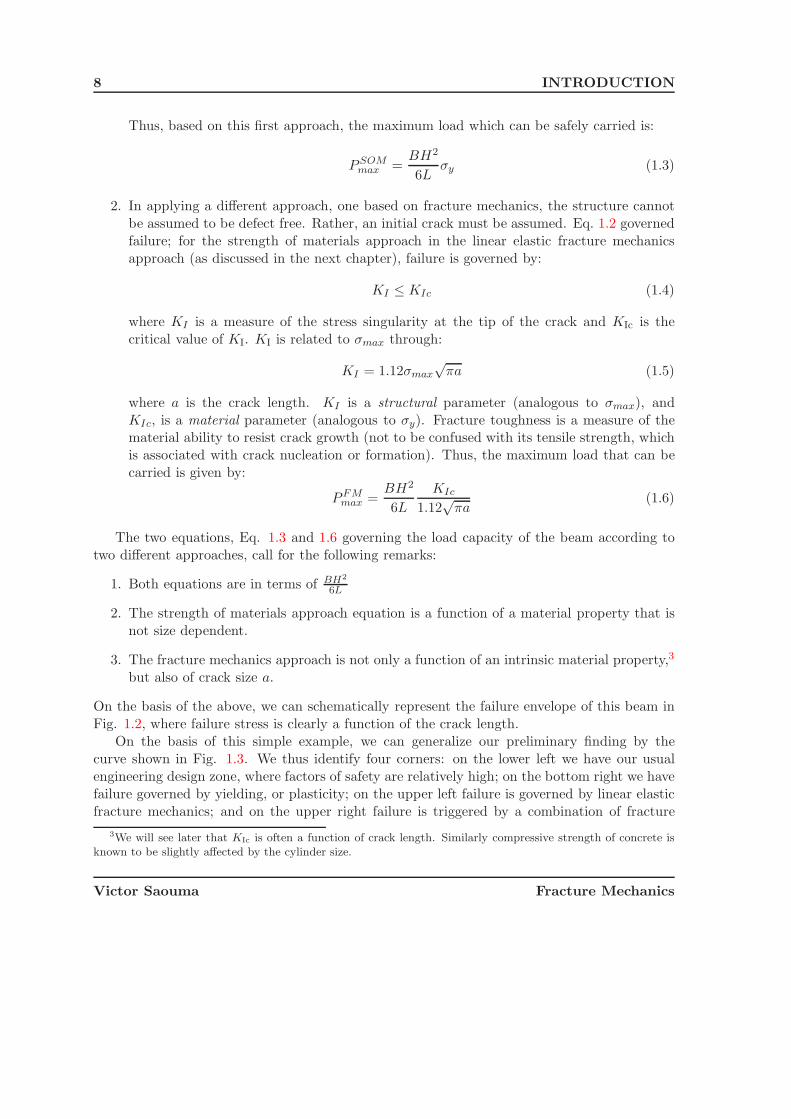
Thus, based on this first approach, the maximum load which can be safely carried is:
PSOMmax =
BH2
6Lσy (1.3)
2. In applying a different approach, one based on fracture mechanics, the structure cannotbe assumed to be defect free. Rather, an initial crack must be assumed. Eq. 1.2 governedfailure; for the strength of materials approach in the linear elastic fracture mechanicsapproach (as discussed in the next chapter), failure is governed by:
KI ≤ KIc (1.4)
where KI is a measure of the stress singularity at the tip of the crack and KIc is thecritical value of KI. KI is related to σmax through:
KI = 1.12σmax√
πa (1.5)
where a is the crack length. KI is a structural parameter (analogous to σmax), andKIc, is a material parameter (analogous to σy). Fracture toughness is a measure of thematerial ability to resist crack growth (not to be confused with its tensile strength, whichis associated with crack nucleation or formation). Thus, the maximum load that can becarried is given by:
PFMmax =
BH2
6L
KIc
1.12√
πa(1.6)
The two equations, Eq. 1.3 and 1.6 governing the load capacity of the beam according totwo different approaches, call for the following remarks:
1. Both equations are in terms of BH2
6L
2. The strength of materials approach equation is a function of a material property that isnot size dependent.
3. The fracture mechanics approach is not only a function of an intrinsic material property,3
but also of crack size a.
On the basis of the above, we can schematically represent the failure envelope of this beam inFig. 1.2, where failure stress is clearly a function of the crack length.
On the basis of this simple example, we can generalize our preliminary finding by thecurve shown in Fig. 1.3. We thus identify four corners: on the lower left we have our usualengineering design zone, where factors of safety are relatively high; on the bottom right we havefailure governed by yielding, or plasticity; on the upper left failure is governed by linear elasticfracture mechanics; and on the upper right failure is triggered by a combination of fracture
3We will see later that KIc is often a function of crack length. Similarly compressive strength of concrete isknown to be slightly affected by the cylinder size.
Victor Saouma Fracture Mechanics

1.3 Fracture Mechanics vs Strength of Materials 9
Figure 1.2: Failure Envelope for a Cracked Cantilevered Beam
mechanics and plasticity. This last zone has been called elasto-plastic in metals, and nonlinearfracture in concrete.4
Finally, we should emphasize that size effect is not unique to fractures but also has beenencountered by most engineers in the design of columns. In fact, depending upon its slendernessratio, a column failure load is governed by either the Euler equation for long columns, or thestrength of materials for short columns.
Column formulas have been developed, as seen in Fig. 1.4, which is similar to Fig. 1.2.Also note that column instability is caused by a not perfectly straight element, whereas fracturefailure is caused by the presence of a crack. In all other cases, a perfect material is assumed, asshown in Table 1.1. As will be shown later, similar transition curves have also been developedby Bazant (Bazant, Z.P. 1984) for the failure of small or large cracked structures on the basisof either strength of materials or linear elastic fracture mechanics.
Approach Governing Eq. Theory Imperfection
Strength of Material σ = PA Plasticity σy Dislocation
Column Instability σ = π2E(KL
r)2
Euler KLr Not Perfectly straight
Fracture σ = Kc√πa
Griffith KIc Micro-defects
Table 1.1: Column Instability Versus Fracture Instability
4This curve will be subsequently developed for concrete materials according to Bazant’s size effect law.
Victor Saouma Fracture Mechanics

10 INTRODUCTION
Figure 1.3: Generalized Failure Envelope
Figure 1.4: Column Curve
Victor Saouma Fracture Mechanics
1.4 Major Historical Developments in Fracture Mechanics 11
1.4 Major Historical Developments in Fracture Mechanics
As with any engineering discipline approached for the first time, it is helpful to put fracturemechanics into perspective by first listing its major developments:
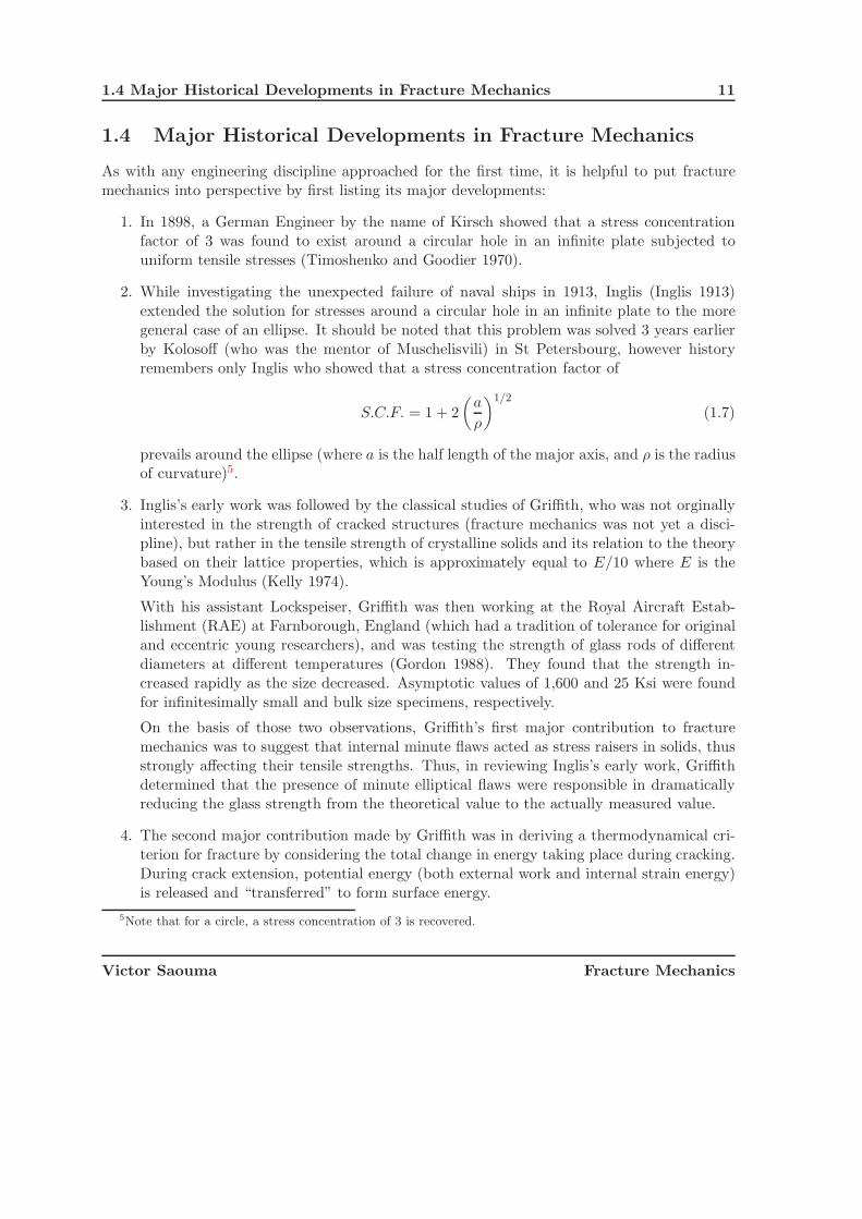
1. In 1898, a German Engineer by the name of Kirsch showed that a stress concentrationfactor of 3 was found to exist around a circular hole in an infinite plate subjected touniform tensile stresses (Timoshenko and Goodier 1970).
2. While investigating the unexpected failure of naval ships in 1913, Inglis (Inglis 1913)extended the solution for stresses around a circular hole in an infinite plate to the moregeneral case of an ellipse. It should be noted that this problem was solved 3 years earlierby Kolosoff (who was the mentor of Muschelisvili) in St Petersbourg, however historyremembers only Inglis who showed that a stress concentration factor of
S.C.F. = 1 + 2
(a
ρ
)1/2
(1.7)
prevails around the ellipse (where a is the half length of the major axis, and ρ is the radiusof curvature)5.
3. Inglis’s early work was followed by the classical studies of Griffith, who was not orginallyinterested in the strength of cracked structures (fracture mechanics was not yet a disci-pline), but rather in the tensile strength of crystalline solids and its relation to the theorybased on their lattice properties, which is approximately equal to E/10 where E is theYoung’s Modulus (Kelly 1974).
With his assistant Lockspeiser, Griffith was then working at the Royal Aircraft Estab-lishment (RAE) at Farnborough, England (which had a tradition of tolerance for originaland eccentric young researchers), and was testing the strength of glass rods of differentdiameters at different temperatures (Gordon 1988). They found that the strength in-creased rapidly as the size decreased. Asymptotic values of 1,600 and 25 Ksi were foundfor infinitesimally small and bulk size specimens, respectively.
On the basis of those two observations, Griffith’s first major contribution to fracturemechanics was to suggest that internal minute flaws acted as stress raisers in solids, thusstrongly affecting their tensile strengths. Thus, in reviewing Inglis’s early work, Griffithdetermined that the presence of minute elliptical flaws were responsible in dramaticallyreducing the glass strength from the theoretical value to the actually measured value.
4. The second major contribution made by Griffith was in deriving a thermodynamical cri-terion for fracture by considering the total change in energy taking place during cracking.During crack extension, potential energy (both external work and internal strain energy)is released and “transferred” to form surface energy.
5Note that for a circle, a stress concentration of 3 is recovered.
Victor Saouma Fracture Mechanics

12 INTRODUCTION
Unfortunately, one night Lockspeiser forgot to turn off the gas torch used for glass melting,resulting in a fire. Following an investigation, (RAE) decided that Griffith should stopwasting his time, and he was transferred to the engine department.
5. After Griffith’s work, the subject of fracture mechanics was relatively dormant for about20 years until 1939 when Westergaard (Westergaard 1939a) derived an expression for thestress field near a sharp crack tip.
6. Up to this point, fracture mechanics was still a relatively obscure and esoteric science.However, more than any other single factor, the large number of sudden and catastrophicfractures that occurred in ships during and following World War II gave the impetus forthe development of fracture mechanics. Of approximately 5,000 welded ships constructedduring the war, over 1,000 suffered structural damage, with 150 of these being seriouslydamaged, and 10 fractured into two parts. After the war, George Irwin, who was at theU.S. Naval Research Laboratory, made use of Griffith’s idea, and thus set the foundationsof fracture mechanics. He made three major contributions:
(a) He (and independently Orowan) extended the Griffith’s original theory to metals byaccounting for yielding at the crack tip. This resulted in what is sometimes calledthe modified Griffith’s theory.
(b) He altered Westergaard’s general solution by introducing the concept of the stressintensity factor (SIF).
(c) He introduced the concept of energy release rate G
7. Subcritical crack growth was subsequently studied. This form of crack propagation isdriven by either applying repeated loading (fatigue) to a crack, or surround it by a cor-rosive environment. In either case the original crack length, and loading condition, takenseparately, are below their critical value. Paris in 1961 proposed the first empirical equa-tion relating the range of the stress intensity factor to the rate of crack growth.
8. Non-linear considerations were further addressed by Wells, who around 1963 utilized thecrack opening displacement (COD) as the parameter to characterize the strength of acrack in an elasto-plastic solid, and by Rice, who introduce his J integral in 1968 inprobably the second most referenced paper in the field (after Griffith); it introduced apath independent contour line integral that is the rate of change of the potential energyfor an elastic non-linear solid during a unit crack extension.
9. Another major contribution was made by Erdogan and Sih in the mid ’60s when theyintroduced the first model for mixed-mode crack propagation.
10. Other major advances have been made subsequently in a number of subdisciplines offracture mechanics: (i) dynamic crack growth; (ii) fracture of laminates and composites;(iii) numerical techniques; (iv) design philosophies; and others.
Victor Saouma Fracture Mechanics

1.5 Coverage 13
11. In 1976, Hillerborg (Hillerborg, A. and Modeer, M. and Petersson, P.E. 1976a) introducedthe fictitious crack model in which residual tensile stresses can be transmitted across aportion of the crack. Thus a new meaning was given to cracks in cementitious materials.
12. In 1979 Bazant and Cedolin (Bazant, Z.P. and Cedolin, L. 1979) showed that for theobjective analysis of cracked concrete structure, fracture mechanics concepts must beused, and that classical strength of materials models would yield results that are meshsensitive.
This brief overview is designed to make detailed coverage of subsequent topics better un-derstood when put into global perspective.
1.5 Coverage
Following this brief overview, chapter two will provide the reader with a review of elasticity.In particular we shall revisit the major equations needed to analytically solve simple problemsinvolving elliptical holes or sharp cracks.
Those solutions will be presented in detail in chapter three. This chapter, mathematicallythe most challenging, is an important one to understand the mathematical complexity of solu-tions of simple crack problem, and to appreciate the value of numerical based solutions whichwill be discussed later. First Inglis solution of a circular and elliptical hole will be presented,then the problem of a sharp crack in an infinite plate will be solved using the two classicalmethods. The first one is based on Westergaard’s solution, and the second on Williams’s clas-sical paper. Through Westergaard’s solution, we shall introduce the concept of stress intensityfactors, and William’s solution will be extended to cracks along an interface between two dis-similar materials. Also covered in this chapter will be the solutions of a crack in a homogeneousanisotropic solid based on the solution of Sih and Paris.
With the rigorous derivation of the stress field ahead of a crack tip performed, Chapter fourwill formalize the Linear Elastic Fracture Mechanics approach, and show how it can be used insome practical design cases.
A complementary approach to the stress based one, will be presented in chapter five whichdiscusses Energy Methods in linear elastic fracture mechanics. First, we shall thoroughly ex-amine the theoretical strength of crystalline materials and contrast it with the actual one, thenwe will define the energy release rate G, and discuss the duality between the stress based andthe energy based approaches.
Chapter six will extend the simple mode I crack propagation criteria to mixed modes (wherea crack is simultaneously subjected to opening and sliding) by discussing some of the majorcriterions.
Subcritical crack growth, and more specifically fatigue crack growth will be covered inchapter seven.
Elasto-Plastic fracture mechanics, and derivation of the J integral will then be covered inchapter eight. First we will derive expressions for the size of the plastic zone ahead of the cracktip, then criteria for crack growth presented.
Victor Saouma Fracture Mechanics

14 INTRODUCTION
In chapter nine, we shall examine some of the fracture testing techniques, with emphasizeon both metallic and cementitious materials.
Fracture of cementitious material, such as concrete and rock, will be studied in chapter ten.In this extensive chapter, we shall review some of the major models currently investigated, andexamine some applications.
Numerical techniques will then be discussed in chapter eleven. First techniques of modellingthe stress singularity at the crack tip will be examined, followed by methods to extract the stressintensity factors from a finite element analysis and evaluation of J integral will be presented.
The last chapter, twelve, will focus on numerical techniques for cementitious materials.For more detailed coverage, the reader is referred to the numerous excellent books available,
such as Broek (Broek 1986, Broek 1989), Cherepanov (Cherepanov 1979), Kanninen (Kanninenand Popelar 1985), Knott (Knott 1976), Barsom and Rolfe (Barsom and Rolfe 1987), andAnderson’s (Anderson 1995). Finally, a recent book by Bazant (Bazant and Cedolin 1991)covers (among other things) some of the issues related to fracture of concrete.
Victor Saouma Fracture Mechanics

Chapter 2
PRELIMINARYCONSIDERATIONS
Needs some minor editing!
1 Whereas, ideally, an introductory course in Continuum Mechanics should be taken prior to afracture mechanics, this is seldom the case. Most often, students have had a graduate course inAdvanced Strength of Materials, which can only provide limited background to a solid fracturemechanics course.
2 Accordingly, this preliminary chapter (mostly extracted from the author’s lecture notes inContinuum Mechanics) will partially remedy for occasional deficiencies and will be often refer-enced.
3 It should be noted that most, but not all, of the material in this chapter will be subsequentlyreferenced.
2.1 Tensors
4 We now seek to generalize the concept of a vector by introducing the tensor (T), whichessentially exists to operate on vectors v to produce other vectors (or on tensors to produceother tensors!). We designate this operation by T·v or simply Tv.
5 We hereby adopt the dyadic and indicialnotation for tensors as linear vector operators
u = T·v or ui = Tijvj (2.1-a)
u = v·S where S = TT (2.1-b)

16 PRELIMINARY CONSIDERATIONS
6 Whereas a tensor is essentially an operator on vectors (or other tensors), it is also a physicalquantity, independent of any particular coordinate system yet specified most conveniently byreferring to an appropriate system of coordinates.
7 Tensors frequently arise as physical entities whose components are the coefficients of a linearrelationship between vectors.
8 A tensor is classified by the rank or order. A Tensor of order zero is specified in any coordinatesystem by one coordinate and is a scalar (such as temperature). A tensor of order one has threecoordinate components in space, hence it is a vector (such as force). In general 3-D space thenumber of components of a tensor is 3n where n is the order of the tensor.
9 A force and a stress are tensors of order 1 and 2 respectively.
2.1.1 Indicial Notation
10 Whereas the Engineering notation may be the simplest and most intuitive one, it often leadsto long and repetitive equations. Alternatively, the tensor and the dyadic form will lead toshorter and more compact forms.
11 While working on general relativity, Einstein got tired of writing the summation symbol withits range of summation below and above (such as
∑n=3i=1 aijbi) and noted that most of the time
the upper range (n) was equal to the dimension of space (3 for us, 4 for him), and that whenthe summation involved a product of two terms, the summation was over a repeated index (iin our example). Hence, he decided that there is no need to include the summation sign
∑if
there was repeated indices (i), and thus any repeated index is a dummy index and is summedover the range 1 to 3. An index that is not repeated is called free index and assumed to takea value from 1 to 3.
12 Hence, this so called indicial notation is also referred to Einstein’s notation.
13 The following rules define indicial notation:
1. If there is one letter index, that index goes from i to n (range of the tensor). For instance:
ai = ai = � a1 a2 a3 =
⎧⎪⎨⎪⎩
a1
a2
a3
⎫⎪⎬⎪⎭ i = 1, 3 (2.2)
assuming that n = 3.
2. A repeated index will take on all the values of its range, and the resulting tensors summed.For instance:
a1ixi = a11x1 + a12x2 + a13x3 (2.3)
3. Tensor’s order:
Victor Saouma Fracture Mechanics
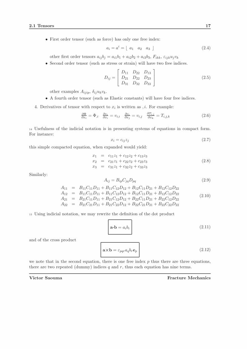
2.1 Tensors 17
• First order tensor (such as force) has only one free index:
ai = ai = � a1 a2 a3 (2.4)
other first order tensors aijbj = ai1b1 + ai2b2 + ai3b3, Fikk, εijkujvk
• Second order tensor (such as stress or strain) will have two free indices.
Dij =
⎡⎢⎣ D11 D22 D13
D21 D22 D23
D31 D32 D33
⎤⎥⎦ (2.5)
other examples Aijip, δijukvk.
• A fourth order tensor (such as Elastic constants) will have four free indices.
4. Derivatives of tensor with respect to xi is written as , i. For example:
∂Φ∂xi
= Φ,i∂vi
∂xi= vi,i
∂vi
∂xj= vi,j
∂Ti,j
∂xk= Ti,j,k (2.6)
14 Usefulness of the indicial notation is in presenting systems of equations in compact form.For instance:
xi = cijzj (2.7)
this simple compacted equation, when expanded would yield:
x1 = c11z1 + c12z2 + c13z3
x2 = c21z1 + c22z2 + c23z3
x3 = c31z1 + c32z2 + c33z3
(2.8)
Similarly:Aij = BipCjqDpq (2.9)
A11 = B11C11D11 + B11C12D12 + B12C11D21 + B12C12D22
A12 = B11C11D11 + B11C12D12 + B12C11D21 + B12C12D22
A21 = B21C11D11 + B21C12D12 + B22C11D21 + B22C12D22
A22 = B21C21D11 + B21C22D12 + B22C21D21 + B22C22D22
(2.10)
15 Using indicial notation, we may rewrite the definition of the dot product
a·b = aibi (2.11)
and of the cross product
a×b = εpqraqbrep (2.12)
we note that in the second equation, there is one free index p thus there are three equations,there are two repeated (dummy) indices q and r, thus each equation has nine terms.
Victor Saouma Fracture Mechanics

18 PRELIMINARY CONSIDERATIONS
2.1.2 Tensor Operations
16 The sum of two (second order) tensors is simply defined as:
Sij = Tij + Uij (2.13)
17 The multiplication of a (second order) tensor by a scalar is defined by:
Sij = λTij (2.14)
18 The inner product is obtained from an outer product by contraction involving one indexfrom each tensor. For example
aibj → aibi (2.15-a)
aiEjk → aiEik = fk (2.15-b)
EijFkm → EijFjm = Gim (2.15-c)
AiB.ki → AiB.k
i = Dk (2.15-d)
19 The scalar product of two tensors is defined as
T : U = TijUij (2.16)
in any rectangular system.
20 The following inner-product axioms are satisfied:
T : U = U : T (2.17-a)
T : (U + V) = T : U + T : V (2.17-b)
α(T : U) = (αT) : U = T : (αU) (2.17-c)
T : T > 0 unless T = 0 (2.17-d)
2.1.3 Rotation of Axes
21 The rule for changing second order tensor components under rotation of axes goes as follow:
ui = ajiuj From Eq. ??
= ajiTjqvq From Eq. 2.1-a
= ajiTjqa
qpvp From Eq. ??
(2.18)
Victor Saouma Fracture Mechanics

2.1 Tensors 19
But we also have ui = T ipvp (again from Eq. 2.1-a) in the barred system, equating these twoexpressions we obtain
T ip − (ajia
qpTjq)vp = 0 (2.19)
hence
T ip = ajia
qpTjq in Matrix Form [T ] = [A]T [T ][A]
Tjq = ajia
qpT ip in Matrix Form [T ] = [A][T ][A]T
(2.20)
By extension, higher order tensors can be similarly transformed from one coordinate system toanother.
22 If we consider the 2D case, From Eq. ??
A =
⎡⎢⎣ cos α sin α 0
− sinα cos α 00 0 1
⎤⎥⎦ (2.21-a)
T =
⎡⎢⎣ Txx Txy 0
Txy Tyy 00 0 0
⎤⎥⎦ (2.21-b)
T = AT TA =
⎡⎢⎣ T xx Txy 0
T xy T yy 00 0 0
⎤⎥⎦ (2.21-c)
=
⎡⎢⎣ cos2 αTxx + sin2 αTyy + sin 2αTxy
12(− sin 2αTxx + sin 2αTyy + 2cos 2αTxy 0
12(− sin 2αTxx + sin 2αTyy + 2cos 2αTxy sin2 αTxx + cos α(cos αTyy − 2 sin αTxy 0
0 0 0
⎤⎥⎦
(2.21-d)
alternatively, using sin 2α = 2 sin α cos α and cos 2α = cos2 α − sin2 α, this last equation canbe rewritten as⎧⎪⎨
⎪⎩T xx
T yy
Txy
⎫⎪⎬⎪⎭ =
⎡⎢⎣ cos2 θ sin2 θ 2 sin θ cos θ
sin2 θ cos2 θ −2 sin θ cos θ− sin θ cos θ cos θ sin θ cos2 θ − sin2 θ
⎤⎥⎦⎧⎪⎨⎪⎩
Txx
Tyy
Txy
⎫⎪⎬⎪⎭ (2.22)
2.1.4 Trace
23 The trace of a second-order tensor, denoted tr T is a scalar invariant function of the tensorand is defined as
tr T ≡ Tii (2.23)
Thus it is equal to the sum of the diagonal elements in a matrix.
Victor Saouma Fracture Mechanics

20 PRELIMINARY CONSIDERATIONS
2.1.5 Inverse Tensor
24 An inverse tensor is simply defined as follows
T−1(Tv) = v and T(T−1v) = v (2.24)
alternatively T−1T = TT−1 = I, or T−1ik Tkj = δij and TikT
−1kj = δij
2.1.6 Principal Values and Directions of Symmetric Second Order Tensors
25 Since the two fundamental tensors in continuum mechanics are of the second order andsymmetric (stress and strain), we examine some important properties of these tensors.
26 For every symmetric tensor Tij defined at some point in space, there is associated with eachdirection (specified by unit normal nj) at that point, a vector given by the inner product
vi = Tijnj (2.25)
If the direction is one for which vi is parallel to ni, the inner product may be expressed as
Tijnj = λni (2.26)
and the direction ni is called principal direction of Tij. Since ni = δijnj, this can be rewrittenas
(Tij − λδij)nj = 0 (2.27)
which represents a system of three equations for the four unknowns ni and λ.
(T11 − λ)n1 + T12n2 + T13n3 = 0
T21n1 + (T22 − λ)n2 + T23n3 = 0 (2.28-a)
T31n1 + T32n2 + (T33 − λ)n3 = 0
To have a non-trivial solution (ni = 0) the determinant of the coefficients must be zero,
|Tij − λδij | = 0 (2.29)
27 Expansion of this determinant leads to the following characteristic equation
λ3 − IT λ2 + IIT λ − IIIT = 0 (2.30)
Victor Saouma Fracture Mechanics
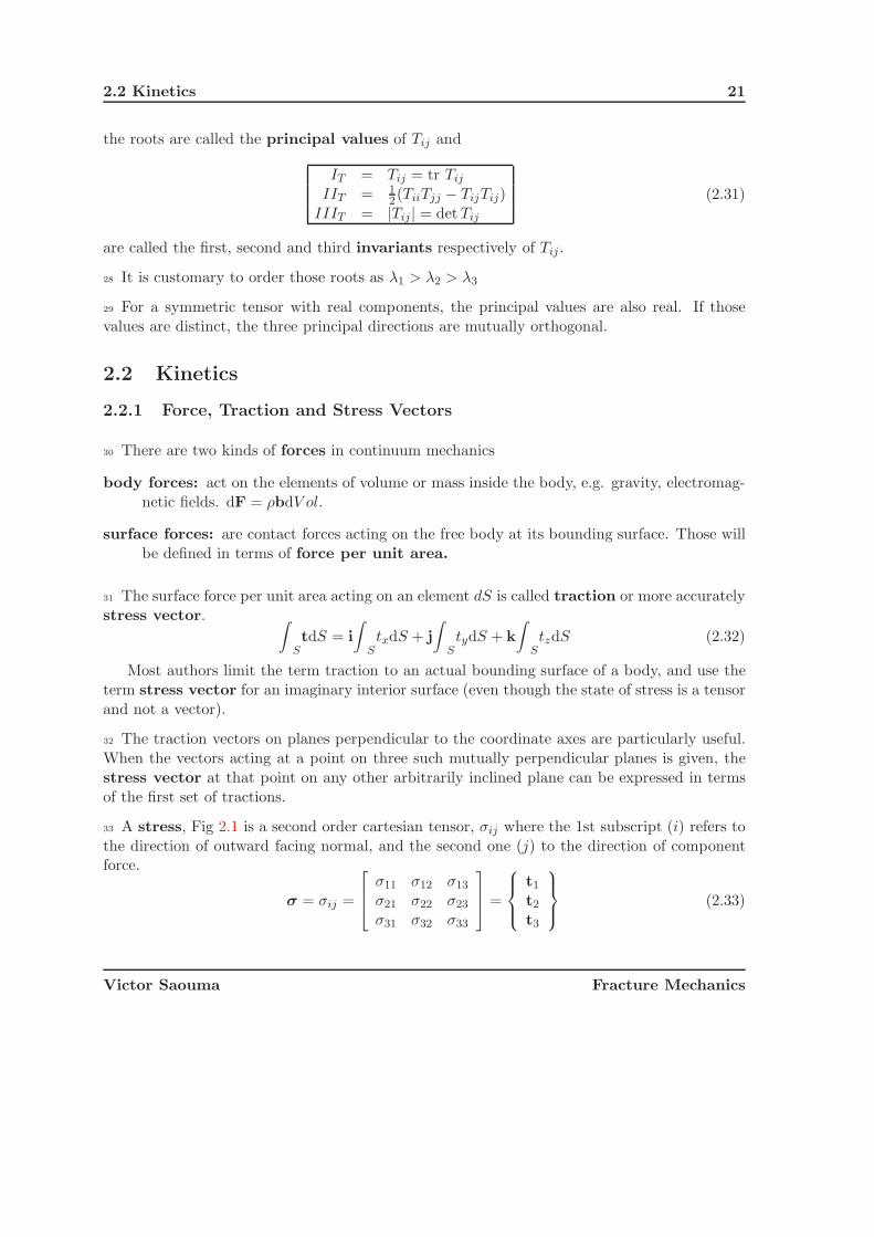
2.2 Kinetics 21
the roots are called the principal values of Tij and
IT = Tij = tr Tij
IIT = 12(TiiTjj − TijTij)
IIIT = |Tij | = det Tij
(2.31)
are called the first, second and third invariants respectively of Tij .
28 It is customary to order those roots as λ1 > λ2 > λ3
29 For a symmetric tensor with real components, the principal values are also real. If thosevalues are distinct, the three principal directions are mutually orthogonal.
2.2 Kinetics
2.2.1 Force, Traction and Stress Vectors
30 There are two kinds of forces in continuum mechanics
body forces: act on the elements of volume or mass inside the body, e.g. gravity, electromag-netic fields. dF = ρbdV ol.
surface forces: are contact forces acting on the free body at its bounding surface. Those willbe defined in terms of force per unit area.
31 The surface force per unit area acting on an element dS is called traction or more accuratelystress vector. ∫
StdS = i
∫StxdS + j
∫StydS + k
∫StzdS (2.32)
Most authors limit the term traction to an actual bounding surface of a body, and use theterm stress vector for an imaginary interior surface (even though the state of stress is a tensorand not a vector).
32 The traction vectors on planes perpendicular to the coordinate axes are particularly useful.When the vectors acting at a point on three such mutually perpendicular planes is given, thestress vector at that point on any other arbitrarily inclined plane can be expressed in termsof the first set of tractions.
33 A stress, Fig 2.1 is a second order cartesian tensor, σij where the 1st subscript (i) refers tothe direction of outward facing normal, and the second one (j) to the direction of componentforce.
σ = σij =
⎡⎢⎣ σ11 σ12 σ13
σ21 σ22 σ23
σ31 σ32 σ33
⎤⎥⎦ =
⎧⎪⎨⎪⎩
t1
t2
t3
⎫⎪⎬⎪⎭ (2.33)
Victor Saouma Fracture Mechanics

22 PRELIMINARY CONSIDERATIONS
2XΔ
X
3X
1
2
X
3
σ
σ
11σ
σ13 21
σ23
σ22
σ31
σ32
σ33
12Δ X 1
Δ X
Figure 2.1: Stress Components on an Infinitesimal Element
34 In fact the nine rectangular components σij of σ turn out to be the three sets of three vectorcomponents (σ11, σ12, σ13), (σ21, σ22, σ23), (σ31, σ32, σ33) which correspond to the three tractionst1, t2 and t3 which are acting on the x1, x2 and x3 faces (It should be noted that those tractionsare not necesarily normal to the faces, and they can be decomposed into a normal and sheartraction if need be). In other words, stresses are nothing else than the components of tractions(stress vector), Fig. 2.2.
35 The state of stress at a point cannot be specified entirely by a single vector with threecomponents; it requires the second-order tensor with all nine components.
2.2.2 Traction on an Arbitrary Plane; Cauchy’s Stress Tensor
36 Let us now consider the problem of determining the traction acting on the surface of anoblique plane (characterized by its normal n) in terms of the known tractions normal to thethree principal axis, t1, t2 and t3. This will be done through the so-called Cauchy’s tetrahedronshown in Fig. 2.3, and will be obtained without any assumption of equilibrium and it will applyin fluid dynamics as well as in solid mechanics.
37 This equation is a vector equation, and the corresponding algebraic equations for the com-ponents of tn are
tn1 = σ11n1 + σ21n2 + σ31n3
tn2 = σ12n1 + σ22n2 + σ32n3
tn3 = σ13n1 + σ23n2 + σ33n3
Indicial notation tni= σjinj
dyadic notation tn = n·σ = σT·n
(2.34)
Victor Saouma Fracture Mechanics

2.2 Kinetics 23
13 σ21
σ23
σ22
σ31
1
σ33
σ32
X 2
X1
V1
X3
X 2
(Components of a vector are scalars)
V
V
V2
X
3
(Components of a tensor of order 2 are vectors)
X3
11σ
σ12
σ
Stresses as components of a traction vector
t
t
t 1
2
3
Figure 2.2: Stresses as Tensor Components
b* Δ V
-t Δ S*
11
*
ρ
S
X
X
X
3
1
2
Oh
n
B
n
C
AN
-t
*
2 ΔS
2
*-t*
3Δ S 3
t Δ
Figure 2.3: Cauchy’s Tetrahedron
Victor Saouma Fracture Mechanics

24 PRELIMINARY CONSIDERATIONS
38 We have thus established that the nine components σij are components of the second ordertensor, Cauchy’s stress tensor.
Example 2-1: Stress Vectors
if the stress tensor at point P is given by
σ =
⎡⎢⎣ 7 −5 0
−5 3 10 1 2
⎤⎥⎦ =
⎧⎪⎨⎪⎩
t1
t2
t3
⎫⎪⎬⎪⎭ (2.35)
We seek to determine the traction (or stress vector) t passing through P and parallel to theplane ABC where A(4, 0, 0), B(0, 2, 0) and C(0, 0, 6).Solution:The vector normal to the plane can be found by taking the cross products of vectors AB andAC:
N = AB×AC =
∣∣∣∣∣∣∣e1 e2 e3
−4 2 0−4 0 6
∣∣∣∣∣∣∣ (2.36-a)
= 12e1 + 24e2 + 8e3 (2.36-b)
The unit normal of N is given by
n =3
7e1 +
6
7e2 +
2
7e3 (2.37)
Hence the stress vector (traction) will be
� 37
67
27
⎡⎢⎣ 7 −5 0
−5 3 10 1 2
⎤⎥⎦ = � −9
757
107 (2.38)
and thus t = −97e1 + 5
7e2 + 107 e3
2.2.3 Invariants
39 The principal stresses are physical quantities, whose values do not depend on the coordinatesystem in which the components of the stress were initially given. They are therefore invariantsof the stress state.
40 When the determinant in the characteristic equation is expanded, the cubic equation takesthe form
λ3 − Iσλ2 − IIσλ − IIIσ = 0 (2.39)
Victor Saouma Fracture Mechanics

2.2 Kinetics 25
where the symbols Iσ, IIσ and IIIσ denote the following scalar expressions in the stress com-ponents:
Iσ = σ11 + σ22 + σ33 = σii = tr σ
IIσ = −(σ11σ22 + σ22σ33 + σ33σ11) + σ223 + σ2
31 + σ212
= 12 (σijσij − σiiσjj) = 1
2σijσij − 12I2
σ
= 12 (σ : σ − I2
σ)IIIσ = detσ = 1
6eijkepqrσipσjqσkr
(2.40)
41 In terms of the principal stresses, those invariants can be simplified into
Iσ = σ(1) + σ(2) + σ(3)
IIσ = −(σ(1)σ(2) + σ(2)σ(3) + σ(3)σ(1))
IIIσ = σ(1)σ(2)σ(3)
(2.41)
2.2.4 Spherical and Deviatoric Stress Tensors
42 If we let σ denote the mean normal stress p
σ = −p =1
3(σ11 + σ22 + σ33) =
1
3σii =
1
3tr σ (2.42)
then the stress tensor can be written as the sum of two tensors:
Hydrostatic stress in which each normal stress is equal to −p and the shear stresses are zero.The hydrostatic stress produces volume change without change in shape in an isotropicmedium.
σhyd = −pI =
⎡⎢⎣ −p 0 0
0 −p 00 0 −p
⎤⎥⎦ (2.43)
Deviatoric Stress: which causes the change in shape.
σdev =
⎡⎢⎣ σ11 − σ σ12 σ13
σ21 σ22 − σ σ23
σ31 σ32 σ33 − σ
⎤⎥⎦ (2.44)
2.2.5 Stress Transformation
43 From Eq. 2.20 and 2.20, the stress transformation for the second order stress tensor is givenby
σip = ajia
qpσjq in Matrix Form [σ] = [A]T [σ][A]
σjq = ajia
qpσip in Matrix Form [σ] = [A][σ][A]T
(2.45)
Victor Saouma Fracture Mechanics

26 PRELIMINARY CONSIDERATIONS
44 For the 2D plane stress case we rewrite Eq. 2.22⎧⎪⎨⎪⎩
σxx
σyy
σxy
⎫⎪⎬⎪⎭ =
⎡⎢⎣ cos2 α sin2 α 2 sin α cos α
sin2 α cos2 α −2 sin α cos α− sinα cos α cos α sin α cos2 α − sin2 α
⎤⎥⎦⎧⎪⎨⎪⎩
σxx
σyy
σxy
⎫⎪⎬⎪⎭ (2.46)
2.2.6 Polar Coordinates
It is often necessary to express cartesian stresses in terms of polar stresses and vice versa. Thiscan be done through the following relationships
σxx = σrr cos2 θ + σθθ sin2 θ − σrθ sin 2θ (2.47-a)
σyy = σrr sin2 θ + σθθ cos2 θ + σrθ sin 2θ (2.47-b)
σxy = (σrr − σθθ) sin θ cos θ + σrθ(cos2 θ − sin2 θ) (2.47-c)
and
σrr =
(σxx + σyy
2
)(1 − a2
r2
)+
(σxx − σyy
2
)(1 +
3a4
r4− 4a2
r2
)cos 2θ
+σxy
(1 +
3a4
r4− 4a2
r2
)sin 2θ (2.48-a)
σθθ =
(σxx + σyy
2
)(1 +
a2
r2
)−(
σxx − σyy
2
)(1 +
3a4
r4
)cos 2θ
−σxy
(1 +
3a4
r4
)sin 2θ (2.48-b)
σrθ = −(
σxx − σyy
2
)(1 − 3a4
r4+
2a2
r2
)sin 2θ + σxy
(1 − 3a4
r4+
2a2
r2
)cos 2θ (2.48-c)
2.3 Kinematic
2.3.1 Strain Tensors
45 The Lagrangian finite strain tensor can be written as
Eij =1
2
(∂ui
∂Xj+
∂uj
∂Xi+
∂uk
∂Xi
∂uk
∂Xj
)or E =
1
2(u∇X + ∇Xu︸ ︷︷ ︸
J+Jc
+ ∇Xu·u∇X︸ ︷︷ ︸Jc·J
) (2.49)
or:
E11 =∂u1
∂X1+
1
2
[(∂u1
∂X1
)2
+
(∂u2
∂X1
)2
+
(∂u3
∂X1
)2]
(2.50-a)
Victor Saouma Fracture Mechanics

2.3 Kinematic 27
E12 =1
2
(∂u1
∂X2+
∂u2
∂X1
)+
1
2
[∂u1
∂X1
∂u1
∂X2+
∂u2
∂X1
∂u2
∂X2+
∂u3
∂X1
∂u3
∂X2
](2.50-b)
· · · = · · · (2.50-c)
46 The Eulerian finite strain tensor can be written as
E∗ij =
1
2
(∂ui
∂xj+
∂uj
∂xi− ∂uk
∂xi
∂uk
∂xj
)or E∗ =
1
2(u∇x + ∇xu︸ ︷︷ ︸
K+Kc
−∇xu·u∇x︸ ︷︷ ︸Kc·K
) (2.51)
47 Expanding
E∗11 =
∂u1
∂x1− 1
2
[(∂u1
∂x1
)2
+
(∂u2
∂x1
)2
+
(∂u3
∂x1
)2]
(2.52-a)
E∗12 =
1
2
(∂u1
∂x2+
∂u2
∂x1
)− 1
2
[∂u1
∂x1
∂u1
∂x2+
∂u2
∂x1
∂u2
∂x2+
∂u3
∂x1
∂u3
∂x2
](2.52-b)
· · · = · · · (2.52-c)
48 Alternatively these equations may be expanded as
εxx = ∂u∂x + 1
2
[(∂u∂x
)2+(
∂v∂x
)2+(
∂w∂x
)2]
εyy = ∂v∂y + 1
2
[(∂u∂y
)2+(
∂v∂y
)2+(
∂w∂y
)2]
εzz = ∂w∂z + 1
2
[(∂u∂z
)2+(
∂v∂z
)2+(
∂w∂z
)2]
εxy = 12
(∂v∂x + ∂u
∂y + ∂u∂x
∂u∂y + ∂v
∂x∂v∂y + ∂w
∂x∂w∂y
)εxz = 1
2
(∂w∂x + ∂u
∂z + ∂u∂x
∂u∂z + ∂v
∂x∂v∂z + ∂w
∂x∂w∂z
)εyz = 1
2
(∂w∂y + ∂v
∂z + ∂u∂y
∂u∂z + ∂v
∂y∂v∂z + ∂w
∂y∂w∂z
)
(2.53)
or
εij =1
2(ui,j + uj,i + uk,iuk,j) (2.54)
From this equation, we note that:
1. We define the engineering shear strain as
γij = 2εij (i �= j) (2.55)
Victor Saouma Fracture Mechanics

28 PRELIMINARY CONSIDERATIONS
2. If the strains are given, then these strain-displacements provide a system of (6) nonlinearpartial differential equation in terms of the unknown displacements (3).
3. εik is the Green-Lagrange strain tensor.
4. The strains have been expressed in terms of the coordinates x, y, z in the undeformed state,i.e. in the Lagrangian coordinate which is the preferred one in structural mechanics.
5. Alternatively we could have expressed ds′2 − dS2 in terms of coordinates in the deformedstate, i.e. Eulerian coordinates x′, y′, z′, and the resulting strains are referred to as theAlmansi strain which is the preferred one in fluid mechanics.
6. In most cases the deformations are small enough for the quadratic term to be dropped,the resulting equations reduce to
εxx = ∂u∂x
εyy = ∂v∂y
εzz = ∂w∂z
γxy = ∂v∂x + ∂u
∂y
γxz = ∂w∂x + ∂u
∂z
γyz = ∂w∂y + ∂v
∂z
(2.56)
or
εij =1
2(ui,k + uk,i) (2.57)
which is called the Cauchy strain
49 In finite element, the strain is often expressed through the linear operator L
ε = Lu (2.58)
or ⎧⎪⎪⎪⎪⎪⎪⎪⎨⎪⎪⎪⎪⎪⎪⎪⎩
εxx
εyy
εzz
εxy
εxz
εyz
⎫⎪⎪⎪⎪⎪⎪⎪⎬⎪⎪⎪⎪⎪⎪⎪⎭︸ ︷︷ ︸
ε
=
⎡⎢⎢⎢⎢⎢⎢⎢⎢⎣
∂∂x 0 0
0 ∂∂y 0
0 0 ∂∂z
∂∂y
∂∂x 0
∂∂z 0 ∂
∂x
0 ∂∂z
∂∂y
⎤⎥⎥⎥⎥⎥⎥⎥⎥⎦
︸ ︷︷ ︸L
⎧⎪⎨⎪⎩
ux
uy
uz
⎫⎪⎬⎪⎭︸ ︷︷ ︸
u
(2.59)
Victor Saouma Fracture Mechanics

2.4 Fundamental Laws of Continuum Mechanics 29
2.3.2 Compatibility Equation
If εij = 12 (ui,j + uj,i) then we have six differential equations (in 3D the strain tensor has a
total of 9 terms, but due to symmetry, there are 6 independent ones) for determining (uponintegration) three unknowns displacements ui. Hence the system is overdetermined, and theremust be some linear relations between the strains.
It can be shown (through appropriate successive differentiation of Eq. ??) that the com-patibility relation for strain reduces to:
∂2εik
∂xj∂xj+
∂2εjj
∂xi∂xk− ∂2εjk
∂xi∂xj− ∂2εij
∂xj∂xk= 0. (2.60)
In 3D, this would yield 9 equations in total, however only six are distinct. In 2D, this resultsin (by setting i = 2, j = 1 and l = 2):
∂2ε11
∂x22
+∂2ε22
∂x21
=∂2γ12
∂x1∂x2(2.61)
(recall that 2ε12 = γ12).When he compatibility equation is written in term of the stresses, it yields:
∂2σ11
∂x22
− ν∂σ22
2
∂x22
+∂2σ22
∂x21
− ν∂2σ11
∂x21
= 2 (1 + ν)∂2σ21
∂x1∂x2(2.62)
2.4 Fundamental Laws of Continuum Mechanics
50 We have thus far studied the stress tensors (Cauchy, Piola Kirchoff), and several other tensorswhich describe strain at a point. In general, those tensors will vary from point to point andrepresent a tensor field.
51 We have also obtained only one differential equation, that was the compatibility equation.
52 In this section, we will derive additional differential equations governing the way stress anddeformation vary at a point and with time. They will apply to any continuous medium, and yetwe will not have enough equations to determine unknown tensor field. For that we need to waitfor the next chapter where constitututive laws relating stress and strain will be introduced.Only with constitutive equations and boundary and initial conditions would we be able toobtain a well defined mathematical problem to solve for the stress and deformation distributionor the displacement or velocity fields.
53 In this chapter we shall derive differential equations expressing locally the conservation ofmass, momentum and energy. These differential equations of balance will be derived fromintegral forms of the equation of balance expressing the fundamental postulates of continuummechanics.
Victor Saouma Fracture Mechanics

30 PRELIMINARY CONSIDERATIONS
2.4.1 Conservation Laws
54 Conservation laws constitute a fundamental component of classical physics. A conservationlaw establishes a balance of a scalar or tensorial quantity in volume V bounded by a surface S.In its most general form, such a law may be expressed as
d
dt
∫VAdV︸ ︷︷ ︸
Rate of variation
+
∫SαdS︸ ︷︷ ︸
Exchange by Diffusion
=
∫VAdV︸ ︷︷ ︸
Source
(2.63)
where A is the volumetric density of the quantity of interest (mass, linear momentum, energy,...) a, A is the rate of volumetric density of what is provided from the outside, and α is therate of surface density of what is lost through the surface S of V and will be a function of thenormal to the surface n.
55 Hence, we read the previous equation as: The input quantity (provided by the right handside) is equal to what is lost across the boundary, and to modify A which is the quantity ofinterest. The dimensions of various quantities are given by
dim(a) = dim(AL−3) (2.64-a)
dim(α) = dim(AL−2t−1) (2.64-b)
dim(A) = dim(AL−3t−1) (2.64-c)
56 Hence, this section will apply the previous conservation law to mass, momentum, and energy.the resulting differential equations will provide additional interesting relation with regard tothe imcompressibiltiy of solids (important in classical hydrodynamics and plasticity theories),equilibrium and symmetry of the stress tensor, and the first law of thermodynamics.
57 The enunciation of the preceding three conservation laws plus the second law of thermo-dynamics, constitute what is commonly known as the fundamental laws of continuummechanics.
2.4.2 Fluxes
58 Prior to the enunciation of the first conservation law, we need to define the concept of fluxacross a bounding surface.
59 The flux across a surface can be graphically defined through the consideration of an imag-inary surface fixed in space with continuous “medium” flowing through it. If we assign apositive side to the surface, and take n in the positive sense, then the volume of “material”flowing through the infinitesimal surface area dS in time dt is equal to the volume of the cylinderwith base dS and slant height vdt parallel to the velocity vector v, Fig. 2.4 (If v·n is negative,
Victor Saouma Fracture Mechanics

2.4 Fundamental Laws of Continuum Mechanics 31
v
n
dS
vdtv dtn
Figure 2.4: Flux Through Area dS
then the flow is in the negative direction). Hence, we define the volume flux as
Volume Flux =
∫Sv·ndS =
∫SvjnjdS (2.65)
where the last form is for rectangular cartesian components.
60 We can generalize this definition and define the following fluxes per unit area through dS:
Mass Flux =
∫Sρv·ndS =
∫SρvjnjdS
Momentum Flux =
∫Sρv(v·n)dS =
∫SρvkvjnjdS
Kinetic Energy Flux =
∫S
1
2ρv2(v·n)dS =
∫S
1
2ρvivivjnjdS
Heat flux =
∫Sq·ndS =
∫SqjnjdS
Electric flux =
∫SJ·ndS =
∫SJjnjdS
(2.66)
2.4.3 Conservation of Mass; Continuity Equation
dρ
dt+ ρ
∂vi
∂xi= 0 or
dρ
dt+ ρ∇·v = 0 (2.67)
The vector form is independent of any choice of coordinates. This equation shows that thedivergence of the velocity vector field equals (−1/ρ)(dρ/dt) and measures the rate of flow ofmaterial away from the particle and is equal to the unit rate of decrease of density ρ in theneighborhood of the particle.
Victor Saouma Fracture Mechanics

32 PRELIMINARY CONSIDERATIONS
61 If the material is incompressible, so that the density in the neighborhood of each materialparticle remains constant as it moves, then the continuity equation takes the simpler form
∂vi
∂xi= 0 or ∇·v = 0 (2.68)
this is the condition of incompressibility
2.4.4 Linear Momentum Principle; Equation of Motion
62 The momentum principle states that the time rate of change of the total momentum of agiven set of particles equals the vector sum of all external forces acting on the particles of theset, provided Newton’s Third Law applies. The continuum form of this principle is a basicpostulate of continuum mechanics.∫
StdS +
∫V
ρbdV =d
dt
∫VρvdV (2.69)
Then we substitute ti = Tijnj and apply the divergence theorm to obtain∫V
(∂Tij
∂xj+ ρbi
)dV =
∫V
ρdVi
dtdV (2.70-a)
∫V
[∂Tij
∂xj+ ρbi − ρ
dVi
dt
]dV = 0 (2.70-b)
or for an arbitrary volume
∂Tij
∂xj+ ρbi = ρ
dVi
dtor ∇T + ρb = ρ
dV
dt(2.71)
which is Cauchy’s (first) equation of motion, or the linear momentum principle, ormore simply equilibrium equation.
63 When expanded in 3D, this equation yields:
∂T11∂x1
+ ∂T12∂x2
+ ∂T13∂x3
+ ρb1 = 0∂T21∂x1
+ ∂T22∂x2
+ ∂T23∂x3
+ ρb2 = 0∂T31∂x1
+ ∂T32∂x2
+ ∂T33∂x3
+ ρb3 = 0
(2.72)
64 We note that these equations could also have been derived from the free body diagramshown in Fig. 2.5 with the assumption of equilibrium (via Newton’s second law) consideringan infinitesimal element of dimensions dx1 × dx2 × dx3. Writing the summation of forces, willyield
Tij,j + ρbi = 0 (2.73)
where ρ is the density, bi is the body force (including inertia).
Victor Saouma Fracture Mechanics

2.4 Fundamental Laws of Continuum Mechanics 33
σ +δyyδσyy
ydy
τ xy
σσ
σ
+δxx
dy
yy
xx
σδ xx
xdx
τ +δxy
τδ xy d
τ yx
τ +δ
τδy
dyyx
yx
xx
dx
Figure 2.5: Equilibrium of Stresses, Cartesian Coordinates
2.4.5 Moment of Momentum Principle
65 The moment of momentum principle states that the time rate of change of the total momentof momentum of a given set of particles equals the vector sum of the moments of all externalforces acting on the particles of the set.
66 Thus, in the absence of distributed couples (this theory of Cosserat will not be coveredin this course) we postulate the same principle for a continuum as
∫S(r×t)dS +
∫V
(r×ρb)dV =d
dt
∫V
(r×ρv)dV (2.74)
2.4.6 Conservation of Energy; First Principle of Thermodynamics
67 The first principle of thermodynamics relates the work done on a (closed) system and theheat transfer into the system to the change in energy of the system. We shall assume thatthe only energy transfers to the system are by mechanical work done on the system by surfacetraction and body forces, by heat transfer through the boundary.
68 If mechanical quantities only are considered, the principle of conservation of energy forthe continuum may be derived directly from the equation of motion given by Eq. 2.71. This isaccomplished by taking the integral over the volume V of the scalar product between Eq. 2.71
Victor Saouma Fracture Mechanics
34 PRELIMINARY CONSIDERATIONS
and the velocity vi. ∫V
viTji,jdV +
∫V
ρbividV =
∫V
ρvidVi
dtdV (2.75)
Applying the divergence theorem,
dK
dt+
dU
dt=
dW
dt+ Q (2.76)
this equation relates the time rate of change of total mechanical energy of the continuum onthe left side to the rate of work done by the surface and body forces on the right hand side.
69 If both mechanical and non mechanical energies are to be considered, the first principle statesthat the time rate of change of the kinetic plus the internal energy is equal to the sum of therate of work plus all other energies supplied to, or removed from the continuum per unit time(heat, chemical, electromagnetic, etc.).
70 For a thermomechanical continuum, it is customary to express the time rate of change ofinternal energy by the integral expression
dU
dt=
d
dt
∫V
ρudV (2.77)
where u is the internal energy per unit mass or specific internal energy. We note that Uappears only as a differential in the first principle, hence if we really need to evaluate thisquantity, we need to have a reference value for which U will be null. The dimension of U is oneof energy dim U = ML2T−2, and the SI unit is the Joule, similarly dim u = L2T−2 with theSI unit of Joule/Kg.
2.5 Constitutive Equations
ceiinosssttuuHooke, 1676
Ut tensio sic visHooke, 1678
71 The Generalized Hooke’s Law can be written as:
σij = Dijklεkl i, j, k, l = 1, 2, 3 (2.78)
72 The (fourth order) tensor of elastic constants Dijkl has 81 (34) components however, due to
the symmetry of both σ and ε, there are at most 36(
9(9−1)2
)distinct elastic terms.
Victor Saouma Fracture Mechanics

2.5 Constitutive Equations 35
73 For the purpose of writing Hooke’s Law, the double indexed system is often replaced by asimple indexed system with a range of six:
σk =
62=36︷ ︸︸ ︷Dkm εm k,m = 1, 2, 3, 4, 5, 6 (2.79)
74 In terms of Lame’s constants, Hooke’s Law for an isotropic body is written as
Tij = λδijEkk + 2μEij or T = λIE + 2μE
Eij = 12μ
(Tij − λ
3λ+2μδijTkk
)or E = −λ
2μ(3λ+2μ) IT + 12μT
(2.80)
75 In terms of engineering constants:
1
E= λ+μ
μ(3λ+2μ) ; ν = λ2(λ+μ)
λ = νE(1+ν)(1−2ν) ; μ = G = E
2(1+ν)
(2.81)
76 Similarly in the case of pure shear in the x1x3 and x2x3 planes, we have
σ21 = σ12 = τ all other σij = 0 (2.82-a)
2ε12 =τ
G(2.82-b)
and the μ is equal to the shear modulus G.
77 Hooke’s law for isotropic material in terms of engineering constants becomes
σij = E1+ν
(εij + ν
1−2ν δijεkk
)or σ = E
1+ν
(ε + ν
1−2ν Iε
)εij = 1+ν
E σij − νE δijσkk or ε = 1+ν
E σ − νE Iσ
(2.83)
78 When the strain equation is expanded in 3D cartesian coordinates it would yield:⎧⎪⎪⎪⎪⎪⎪⎪⎨⎪⎪⎪⎪⎪⎪⎪⎩
εxx
εyy
εzz
γxy(2εxy)γyz(2εyz)γzx(2εzx)
⎫⎪⎪⎪⎪⎪⎪⎪⎬⎪⎪⎪⎪⎪⎪⎪⎭
=1
E
⎡⎢⎢⎢⎢⎢⎢⎢⎣
1 −ν −ν 0 0 0−ν 1 −ν 0 0 0−ν −ν 1 0 0 00 0 0 1 + ν 0 00 0 0 0 1 + ν 00 0 0 0 0 1 + ν
⎤⎥⎥⎥⎥⎥⎥⎥⎦
⎧⎪⎪⎪⎪⎪⎪⎪⎨⎪⎪⎪⎪⎪⎪⎪⎩
σxx
σyy
σzz
τxy
τyz
τzx
⎫⎪⎪⎪⎪⎪⎪⎪⎬⎪⎪⎪⎪⎪⎪⎪⎭
(2.84)
79 If we invert this equation, we obtain⎧⎪⎪⎪⎪⎪⎪⎪⎨⎪⎪⎪⎪⎪⎪⎪⎩
σxx
σyy
σzz
τxy
τyz
τzx
⎫⎪⎪⎪⎪⎪⎪⎪⎬⎪⎪⎪⎪⎪⎪⎪⎭
=
⎡⎢⎢⎢⎢⎢⎢⎢⎢⎣
E(1+ν)(1−2ν)
⎡⎢⎣ 1 − ν ν ν
ν 1 − ν νν ν 1 − ν
⎤⎥⎦ 0
0 G
⎡⎢⎣ 1 0 0
0 1 00 0 1
⎤⎥⎦
⎤⎥⎥⎥⎥⎥⎥⎥⎥⎦
⎧⎪⎪⎪⎪⎪⎪⎪⎨⎪⎪⎪⎪⎪⎪⎪⎩
εxx
εyy
εzz
γxy(2εxy)γyz(2εyz)γzx(2εzx)
⎫⎪⎪⎪⎪⎪⎪⎪⎬⎪⎪⎪⎪⎪⎪⎪⎭(2.85)
Victor Saouma Fracture Mechanics

36 PRELIMINARY CONSIDERATIONS
2.5.1 Transversly Isotropic Case
80 For transversely isotropic, we can express the stress-strain relation in tems of
εxx = a11σxx + a12σyy + a13σzz
εyy = a12σxx + a11σyy + a13σzz
εzz = a13(σxx + σyy) + a33σzz
γxy = 2(a11 − a12)τxy
γyz = a44τxy
γxz = a44τxz
(2.86)
and
a11 =1
E; a12 = − ν
E; a13 = − ν ′
E′ ; a33 = − 1
E′ ; a44 = − 1
μ′ (2.87)
where E is the Young’s modulus in the plane of isotropy and E′ the one in the plane normalto it. ν corresponds to the transverse contraction in the plane of isotropy when tension isapplied in the plane; ν ′ corresponding to the transverse contraction in the plane of isotropywhen tension is applied normal to the plane; μ′ corresponding to the shear moduli for the planeof isotropy and any plane normal to it, and μ is shear moduli for the plane of isotropy.
2.5.2 Special 2D Cases
81 Often times one can make simplifying assumptions to reduce a 3D problem into a 2D one.
2.5.2.1 Plane Strain
82 For problems involving a long body in the z direction with no variation in load or geometry,then εzz = γyz = γxz = τxz = τyz = 0. Thus, replacing into Eq. 2.85 we obtain⎧⎪⎪⎪⎨
⎪⎪⎪⎩σxx
σyy
σzz
τxy
⎫⎪⎪⎪⎬⎪⎪⎪⎭ =
E
(1 + ν)(1 − 2ν)
⎡⎢⎢⎢⎣
(1 − ν) ν 0ν (1 − ν) 0ν ν 00 0 1−2ν
2
⎤⎥⎥⎥⎦⎧⎪⎨⎪⎩
εxx
εyy
γxy
⎫⎪⎬⎪⎭ (2.88)
2.5.2.2 Axisymmetry
83 In solids of revolution, we can use a polar coordinate sytem and
εrr =∂u
∂r(2.89-a)
εθθ =u
r(2.89-b)
Victor Saouma Fracture Mechanics
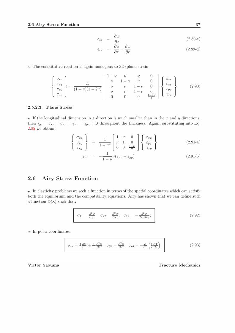
2.6 Airy Stress Function 37
εzz =∂w
∂z(2.89-c)
εrz =∂u
∂z+
∂w
∂r(2.89-d)
84 The constitutive relation is again analogous to 3D/plane strain
⎧⎪⎪⎪⎨⎪⎪⎪⎩
σrr
σzz
σθθ
τrz
⎫⎪⎪⎪⎬⎪⎪⎪⎭ =
E
(1 + ν)(1 − 2ν)
⎡⎢⎢⎢⎢⎢⎣
1 − ν ν ν 0ν 1 − ν ν 0ν ν 1 − ν 0ν ν 1 − ν 00 0 0 1−2ν
2
⎤⎥⎥⎥⎥⎥⎦
⎧⎪⎪⎪⎨⎪⎪⎪⎩
εrr
εzz
εθθ
γrz
⎫⎪⎪⎪⎬⎪⎪⎪⎭ (2.90)
2.5.2.3 Plane Stress
85 If the longitudinal dimension in z direction is much smaller than in the x and y directions,then τyz = τxz = σzz = γxz = γyz = 0 throughout the thickness. Again, substituting into Eq.2.85 we obtain: ⎧⎪⎨
⎪⎩σxx
σyy
τxy
⎫⎪⎬⎪⎭ =
1
1 − ν2
⎡⎢⎣ 1 ν 0
ν 1 00 0 1−ν
2
⎤⎥⎦⎧⎪⎨⎪⎩
εxx
εyy
γxy
⎫⎪⎬⎪⎭ (2.91-a)
εzz = − 1
1 − νν(εxx + εyy) (2.91-b)
2.6 Airy Stress Function
86 In elasticity problems we seek a function in terms of the spatial coordinates which can satisfyboth the equilibrium and the compatibility equations. Airy has shown that we can define sucha function Φ(x) such that:
σ11 = ∂2Φ∂x2
2; σ22 = ∂2Φ
∂x21; σ12 = − ∂2Φ
∂x1∂x2; (2.92)
87 In polar coordinates:
σrr = 1r
∂Φ∂r + 1
r2∂2Φ∂θ2 σθθ = ∂2Φ
∂r2 σrθ = − ∂∂r
(1r
∂Φ∂θ
)(2.93)
Victor Saouma Fracture Mechanics

38 PRELIMINARY CONSIDERATIONS
It can be shown (by direct substitution of these equations in Eq. 2.72) that the equilibriumequation is automatically satisfied.
88 For linear elastic isotropic materials, the satisfaction of the compatibility equation (Eq. 2.62)further requires that Φ must be such that
∇2(∇2Φ
)≡(
∂2
∂x21
+∂2
∂x22
)(∂2Φ
∂x21
+∂2Φ
∂x22
)=
∂4Φ
∂x41
+ 2∂4Φ
∂x21∂x2
2
+∂4Φ
∂x42
= 0 (2.94)
where ∇2 is the Laplacian operator. A solution to Laplace’s equation is referred to as aharmonic function.
89 In polar coordinates
∇2(∇2Φ
)=
(∂2
∂r2+
1
r
∂
∂r+
1
r2
∂2
∂θ2
)(∂2Φ
∂r2+
1
r
∂Φ
∂r+
1
r2
∂2Φ
∂θ2
)(2.95)
90 Thus, the Airy stress function will enable us to solve elasticity problems provided we cancome up with the right choice for Φ which satisfies the natural boundary conditions (stresses).
2.7 Complex Variables
91 As will be shown in the next chapter, we can use Airy stress function with real variablesto determine the stress field around a circular hole, however we need to extend Airy stressfunctions to complex variables in order to analyze: 1) stresses around an elliptical hole (Inglis),and stresses at the tip of a crack (Westergaard).
92 First we define the complex number z as:
z = x1 + ix2 = reiθ (2.96)
where i =√−1, x1 and x2 are the cartesian coordinates, and r and θ are the polar coordinates.
93 We further define an analytic function, f(z) one which derivatives depend only on z.Applying the chain rule
∂
∂x1f(z) =
∂
∂zf(z)
∂z
∂x1= f ′(z)
∂z
∂x1= f ′(z) (2.97-a)
∂
∂x2f(z) =
∂
∂zf(z)
∂z
∂x2= f ′(z)
∂z
∂x2= if ′(z) (2.97-b)
Victor Saouma Fracture Mechanics

2.7 Complex Variables 39
94 If f(z) = α + iβ where α and β are real functions of x1 and x2, and f(z) is analytic, thenfrom Eq. 2.97-a and 2.97-b we have:
∂f(z)∂x1
= ∂α∂x1
+ i ∂β∂x1
= f ′(z)∂f(z)∂x2
= ∂α∂x2
+ i ∂β∂x2
= if ′(z)
}i
(∂α
∂x1+ i
∂β
∂x1
)︸ ︷︷ ︸
i1st Equation
=∂α
∂x2+ i
∂β
∂x2︸ ︷︷ ︸2nd Equation
(2.98)
95 Equating the real and imaginary parts yields the Cauchy-Riemann equations:
∂α
∂x1=
∂β
∂x2;
∂α
∂x2= − ∂β
∂x1
(2.99)
96 If we differentiate those two equation, first with respect to x1, then with respect to x2, andthen add them up we obtain
∂2α
∂x21
+∂2α
∂x22
= 0 or ∇2 (α) = 0 (2.100)
which is Laplace’s equation.
97 Similarly we can have:∇2 (β) = 0 (2.101)
Hence both the real (α) and the imaginary part (β) of an analytic function will separatelyprovide solution to Laplace’s equation, and α and β are conjugate harmonic functions.
2.7.1 Complex Airy Stress Functions
98 It can be shown that any stress function can be expressed as
Φ = Re[(x1 − ix2)ψ(z) + χ(z)] (2.102)
provided that both ψ(z) (psi) and χ(z) (chi) are harmonic (i.e ∇2(ψ) = ∇2(χ) = 0) analyticfunctions of x1 and x2. ψ and χ are often referred to as the Kolonov-Muskhelishvili complexpotentials.
99 If f(z) = α + iβ and both α and β are real, then its conjugate function is defined as:
f(z) = α − iβ (2.103)
Victor Saouma Fracture Mechanics

40 PRELIMINARY CONSIDERATIONS
100 Note that conjugate functions should not be confused with the conjugate harmonic functions.Hence we can rewrite Eq. 2.102 as:
Φ = Re[zψ(z) + χ(z)] (2.104)
101 Substituting Eq. 2.104 into Eq. 2.92, we can determine the stresses
σ11 + σ22 = 4Reψ′(z)σ22 − σ11 + 2iσ12 = 2[zψ′′(z) + χ′′(z)]
(2.105)
and by separation of real and imaginary parts we can then solve for σ22 − σ11 & σ12.
102 Displacements can be similarly obtained.
2.8 Curvilinear Coordinates
103 A variable z = x1 + ix2 in the cartesian coordinate system can be expressed as reiθ in polarcoordinate systems, and as p = α + iβ in curvilinear system.
104 Next, we seek to solve for x1 and x2 in terms of α and β. The relationship between z andp is given by
z = c cosh p (2.106)
where c is a constant.
105 Recalling that
cosh α =1
2(eα + e−α) (2.107-a)
sinhα =1
2(eα − e−α) (2.107-b)
eiβ = cos β + i sin β (2.107-c)
we substitute those equations into Eq. 2.106
x1 + ix2 =c
2
(eα+iβ + e−α−iβ
)=
c
2
(eα cos β + ieα sin β︸ ︷︷ ︸+ e−α cos β − ie−α sin β︸ ︷︷ ︸
)= cos β (eα + e−α)︸ ︷︷ ︸
2 cosh α
+i sin β (eα − e−α)︸ ︷︷ ︸2 sinh α
= c(cosh α cos β + i sinhα sinβ) (2.108-a)
Victor Saouma Fracture Mechanics

2.8 Curvilinear Coordinates 41
Figure 2.6: Curvilinear Coordinates
106 Separating reals from immaginary parts we obtain
x1 = c cosh α cos β = c2 cos β(eα + e−α)
x2 = c sinhα sinβ = c2 sin β(eα − e−α)
(2.109)
107 If we eliminate β from those equation, we obtain
x21
cosh2 α+
x22
sinh2 α= c2 (2.110)
108 Thus for a constant value of α this represents the equation of an ellipse in the x1−x2 plane.Similarly lines of constant β represent confocal hyperebolae which intersect the ellipse at rightangle, Fig. 2.6.
109 In terms of complex potentials, it can be shown that the stresses are given in an analogousway as in Eq. 2.105:
σαα + σββ = 2[ψ′(z) + ψ′(z)] = 4Reψ′(z)σββ − σαα + 2iσαβ = 2e2iθ[zψ′′(z) + ψ′′(z)]
(2.111)
Note that what we have here is a set of three equations in terms of three unknowns.
110 Individual stresses are obtained by separating the real from the imaginary components.
Victor Saouma Fracture Mechanics

42 PRELIMINARY CONSIDERATIONS
2.9 Basic Equations of Anisotropic Elasticity
111 An alternate form of Eq. 2.78 isεi = aijσj (2.112)
where the indices i and j go from 1 to 6.
112 In the most general case this would yield 36 independent constants aij, (Lekhnitskii 1981),
however by virtue of symmetry (aij = aji) this reduces to 21(
(7)(6)2
). If the the material
has one plane of elastic symmetry, then there would 13 independent constants; If it has threemutually orthogonal planes of elastic symmetry, then we would say that it is orthogonallyanisotropic or orthotropic, and we will have a16 = a26 = a36 = a45 = 0, thus there will be 9independent constants.⎧⎪⎪⎪⎪⎪⎪⎪⎨
⎪⎪⎪⎪⎪⎪⎪⎩
ε1
ε2
ε3
ε4
ε5
ε6
⎫⎪⎪⎪⎪⎪⎪⎪⎬⎪⎪⎪⎪⎪⎪⎪⎭
=
⎡⎢⎢⎢⎢⎢⎢⎢⎣
a11 a12 a13
a22 a23
a33
a44
a55
a66
⎤⎥⎥⎥⎥⎥⎥⎥⎦
⎧⎪⎪⎪⎪⎪⎪⎪⎨⎪⎪⎪⎪⎪⎪⎪⎩
σ1
σ2
σ3
σ4
σ5
σ6
⎫⎪⎪⎪⎪⎪⎪⎪⎬⎪⎪⎪⎪⎪⎪⎪⎭
(2.113)
113 If the material is transversally isotropic then it will have 5 independent constants, Fig. 2.7,⎧⎪⎪⎪⎪⎪⎪⎪⎨⎪⎪⎪⎪⎪⎪⎪⎩
ε1
ε2
ε3
ε4
ε5
ε6
⎫⎪⎪⎪⎪⎪⎪⎪⎬⎪⎪⎪⎪⎪⎪⎪⎭
=
⎡⎢⎢⎢⎢⎢⎢⎢⎣
a11 a12 a13
a11 a13
a33
2(a11 − a12)a44
a44
⎤⎥⎥⎥⎥⎥⎥⎥⎦
⎧⎪⎪⎪⎪⎪⎪⎪⎨⎪⎪⎪⎪⎪⎪⎪⎩
σ1
σ2
σ3
σ4
σ5
σ6
⎫⎪⎪⎪⎪⎪⎪⎪⎬⎪⎪⎪⎪⎪⎪⎪⎭
(2.114)
114 The total number of coefficients for different materials is summarized in Table 2.1.
Class of Material Number of Non Zero Coeff. Number of Indep. Coeff.3D 2D 3D 2D
General Anisotropy 36 9 21 6One plane of Symmetry 20 9 13 6Orthotropic 12 5 9 4Transversely Isotropic 12 5 5 4
Isotropic 12 5 2 2
Table 2.1: Number of Elastic Constants for Different Materials
Victor Saouma Fracture Mechanics

2.9 Basic Equations of Anisotropic Elasticity 43
Figure 2.7: Transversly Isotropic Material
115 In terms of engineering constants for an orthotropic solid we would have
εx =1
E1σx − ν21
E2σy −
ν31
E3σz (2.115-a)
εy = −ν12
E1σx +
1
E2σy −
ν32
E3σz (2.115-b)
εz = −ν13
E1σx − ν23
E2σy +
1
E3σz (2.115-c)
γyz =1
μ23τyz (2.115-d)
γxz =1
μ13τxz (2.115-e)
γxy =1
μ12τxy (2.115-f)
however, of the 12 elastic constants, only 9 are independent because the following relations
E1ν21 = E2ν12 (2.116-a)
E2ν32 = E3ν23 (2.116-b)
E3ν13 = E1ν31 (2.116-c)
116 Note that the preceding equations are written for the principal directions of elasticity, x, y,and z in terms of the principal elastic constants (as opposed to constants in equations foran arbitrary system of coordinates).
117 Whereas very few natural or man-made materials are truly orthotropic (certain crystals astopaz are), a number of others are transversely isotropic. Transversely isotropic have through
Victor Saouma Fracture Mechanics

44 PRELIMINARY CONSIDERATIONS
every point a plane in which all directions are equivalent with respect to elastic properties (suchas in laminates, shist, quartz, roller compacted concrete, etc...). For transversely isotropic solidsin 3D, we have
εx = a11σx + a12σy + a13σz (2.117-a)
εy = a12σx + a11σy + a13σz (2.117-b)
εz = a13(σx + σy) + a33σz (2.117-c)
γxy = 2(a11 − a12)τxy (2.117-d)
γyz = a44τxy (2.117-e)
γxz = a44τxz (2.117-f)
and
a11 =1
E; a12 = − ν
E; a13 = − ν ′
E′ ; a33 = − 1
E′ ; a44 = − 1
μ′ (2.118)
118 Thus we have five elastic constants. Denoting by E the Young’s modulus in the plane ofisotropy and E′ the one in the plane normal to it, we would have ν corresponds to the transversecontraction in the plane of isotropy when tension is applied in the plane; ν ′ corresponding tothe transverse contraction in the plane of isotropy when tension is applied normal to the plane;μ′ corresponding to the shear moduli for the plane of isotropy and any plane normal to it, andμ is shear moduli for the plane of isotropy.
2.9.1 Coordinate Transformations
119 If the elastic constants are to be determined for an arbitrary orientation 1-2, Fig. 2.8 thenthe compliance matrix is given by
[C ′] = [Γ]T [C][Γ] (2.119)
where [Γ] is the usual second order tensor transformation for rotation in a plane.
[Γ] =
⎡⎢⎣ cos2 θ sin2 θ 2 sin θ cos θ
sin2 θ cos2 θ −2 sin θ cos θ− sin θ cos θ cos θ sin θ cos2 θ − sin2 θ
⎤⎥⎦ (2.120)
120 Note that after transformation, a transversely isotropic material will not have anymore 5nonzero coefficients, but 9 in (3-D).
2.9.2 Plane Stress-Strain Compliance Transformation
121 If we consider εi = aijσj for plane strain and εi = bijσj for plane stress then it can be shownthat
bij = aij −ai3aj3
a33(2.121)
Victor Saouma Fracture Mechanics

2.9 Basic Equations of Anisotropic Elasticity 45
Figure 2.8: Coordinate Systems for Stress Transformations
2.9.3 Stress Functions
122 The stress function Φ(x, y) can be written as
Φ(x, y) = 2Re[Φ1(z1) + Φ2(z2] (2.122)
where Φ1(z1) is an arbitrary function of z1 = x + s1y and Φ2(z2) is an arbitrary function ofz2 = x + s2y
123 Note the analogy with φ = Re[(x1 − ix2)ψ(z) + χ(z)] derived earlier for isotropic cases, Eq.2.102, where ψ and χ were the Muskhelisvily complex potentials.
124 It can be shown that using the Airy stress function defined in Eq. 2.92 and combined withthe compatibility Equation (Eq. 2.60) for anisotropic solids we obtain (neglecting body forces)
a22∂4Φ
∂x4− 2a26
∂4Φ
∂x∂y+ (2a12 + a66)
∂4Φ
∂x2∂y2− 2a16
∂4Φ
∂x∂y3+ a11
∂4Φ
∂y4= 0 (2.123)
125 For isotropic material this equation reduces to:
∂4Φ
∂x4+ 2
∂4Φ
∂x2∂y2+
∂4Φ
∂y4= 0 (2.124)
which is Eq. 2.94 as derived earlier.
Victor Saouma Fracture Mechanics

46 PRELIMINARY CONSIDERATIONS
126 The characteristic equation of this homogeneous partial differential equation is
a11s4 − 2a16s
3 + (2a12 + a66)s2 − 2a26s + a22 = 0 (2.125)
127 By energy considerations, Leknitskii, (Lekhnitskii 1981) has shown that:
1. All roots are complex or purely imaginary for an ideally elastic body with a11 �= 0,2a12 + a66 �= 0, & a22 �= 0
2. Only exceptions are:
(a) a22 = a26 = 0 ⇒ 2 roots equal to zero
(b) a22 = a26 = 2a12 + a66 = a16 = 0 ⇒ all four roots are zero
(c) a11 = a16 = 0 ⇒ 2 roots are infinite
(d) a11 = a16 = 2a12 + a66 = a26 = 0 ⇒ 4 roots are infinite.
3. Two of the roots are conjugates of the two others: if we let
s1 = α1 + iβ1 s2 = α2 + iβ2 (2.126-a)
then
s3 = s1 s4 = s2 (2.127-a)
then β1 & β2 are both positive and β1 �= β2
4. Two cases are possible:
(a) Roots are all different
(b) Roots are pairwise equal
5. For isotropic material
α = 0 (2.128-a)
β = 1 (2.128-b)
s1 = s2 = i (2.128-c)
s1 = s2 = −i (2.128-d)
So s1 and s2 are complex parameters of first order of plane stress (or strain). Theycharacterize the degree of anisotropy for plane problems. From it we can judge how mucha body differs from isotropy.
6. If a material is orthotropic and x and y coincide with 1 and 2, then a16 = a26 = 0 and wehave
s4 + (E1
μ− 2ν1)s
2 +E1
E2= 0 (2.129)
and
Victor Saouma Fracture Mechanics

2.9 Basic Equations of Anisotropic Elasticity 47
(a) s1 = βi & s2 = δi; purely imaginary and unequal roots
(b) s1 = s2 = βi; complex and equal roots
(c) s1 = α + βi; s2 = −α + βi
7. In addition we have
s′1 =s2 cos ψ − sin ψ
cos ψ + s1 sin ψ(2.130-a)
s′2 =s1 cos ψ − sin ψ
cos ψ + s2 sin ψ(2.130-b)
8. Invariants for orthotropic bodies are
I1 = a11 + a22 + 2a12 =1
E1+
1
E2− 2ν12
E1(2.131-a)
I2 = a66 − 4a12 =1
μ12+
4ν12
E1(2.131-b)
I3 = a44 + a55 =1
μ13+
1
μ23(2.131-c)
I4 = a13 + a23 = −(ν13
E1+
ν23
E2) = −ν31 + ν32
E2(2.131-d)
2.9.4 Stresses and Displacements
128 If we define:
φ1(z1) =dΦ1
dz1and φ2(z2) =
dΦ2
dz2(2.132)
and using the definition of stress functions, the stresses are
σx = 2Re[s21φ1′(z1) + s2
2φ2′(z2)]σy = 2Re[φ1′(z1) + φ2′(z2)]τxy = −2Re[s1φ1′(z1) + s2φ2′(z2)]
(2.133)
and the displacements are
u = 2Re[p1φ1(z1) + p2φ2(z2)]υ = 2Re[q1φ1(z1) + q2φ2(z2)]
(2.134)
where {pi = a11s
2i + a12 − a16si, (i = 1, 2)
qi = a12si + a22si
− a26(2.135-a)
Victor Saouma Fracture Mechanics

48 PRELIMINARY CONSIDERATIONS
2.10 Conclusion
129 In summary, this chapter has provided the mathematical foundation required to develop thesolutions of some “simple” problems which will be presented in the subsequent chapter.
Victor Saouma Fracture Mechanics

Part II
LINEAR ELASTIC FRACTUREMECHANICS

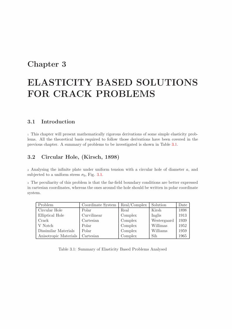
Chapter 3
ELASTICITY BASED SOLUTIONSFOR CRACK PROBLEMS
3.1 Introduction
1 This chapter will present mathematically rigorous derivations of some simple elasticity prob-lems. All the theoretical basis required to follow those derivations have been covered in theprevious chapter. A summary of problems to be investigated is shown in Table 3.1.
3.2 Circular Hole, (Kirsch, 1898)
2 Analysing the infinite plate under uniform tension with a circular hole of diameter a, andsubjected to a uniform stress σ0, Fig. 3.1.
3 The peculiarity of this problem is that the far-field boundary conditions are better expressedin cartesian coordinates, whereas the ones around the hole should be written in polar coordinatesystem.
Problem Coordinate System Real/Complex Solution Date
Circular Hole Polar Real Kirsh 1898Elliptical Hole Curvilinear Complex Inglis 1913Crack Cartesian Complex Westergaard 1939V Notch Polar Complex Willimas 1952Dissimilar Materials Polar Complex Williams 1959Anisotropic Materials Cartesian Complex Sih 1965
Table 3.1: Summary of Elasticity Based Problems Analysed

52 ELASTICITY BASED SOLUTIONS FOR CRACK PROBLEMS
rr
rθ
b
rrσ
I II
bθ
θ
σ
τ
a aa
τrθ
σo
θb
x
σrr
y
σo
Figure 3.1: Circular Hole in an Infinite Plate
4 We will solve this problem by replacing the plate with a thick tube subjected to two differentset of loads. The first one is a thick cylinder subjected to uniform radial pressure (solution ofwhich is well known from Strength of Materials), the second one is a thick cylinder subjectedto both radial and shear stresses which must be compatible with the traction applied on therectangular plate.
5 First we select a stress function which satisfies the biharmonic Equation (Eq. 2.94), and thefar-field boundary conditions. From St Venant principle, away from the hole, the boundaryconditions are given by:
σxx = σ0; σyy = τxy = 0 (3.1)
6 Recalling (Eq. 2.92) that σxx = ∂2Φ∂y2 , this would would suggest a stress function Φ of the form
Φ = σ0y2. Alternatively, the presence of the circular hole would suggest a polar representation
of Φ. Thus, substituting y = r sin θ would result in Φ = σ0r2 sin2 θ.
7 Since sin2 θ = 12(1 − cos 2θ), we could simplify the stress function into
Φ = f(r) cos 2θ (3.2)
8 Substituting this function into the biharmonic equation (Eq. 2.95) yields(∂2
∂r2+
1
r
∂
∂r+
1
r2
∂2
∂θ2
)(∂2Φ
∂r2+
1
r
∂Φ
∂r+
1
r2
∂2Φ
∂θ2
)= 0 (3.3-a)
(d2
dr2+
1
r
d
dr− 4
r2
)(d2f
dr2+
1
r
df
dr− 4f
r2
)= 0 (3.3-b)
(note that the cos 2θ term is dropped)
9 The general solution of this ordinary linear fourth order differential equation is
f(r) = Ar2 + Br4 + C1
r2+ D (3.4)
Victor Saouma Fracture Mechanics

3.2 Circular Hole, (Kirsch, 1898) 53
thus the stress function becomes
Φ =
(Ar2 + Br4 + C
1
r2+ D
)cos 2θ (3.5)
10 Next, we must determine the constants A, B, C, and D. Using Eq. 2.93, the stresses aregiven by
σrr = 1r
∂Φ∂r + 1
r2∂2Φ∂θ2 = −
(2A + 6C
r4 + 4Dr2
)cos 2θ
σθθ = ∂2Φ∂r2 =
(2A + 12Br2 + 6C
r4
)cos 2θ
τrθ = − ∂∂r
(1r
∂Φ∂θ
)=
(2A + 6Br2 − 6C
r4 − 2Dr2
)sin 2θ
(3.6)
11 Next we seek to solve for the four constants of integration by applying the boundary condi-tions. We will identify two sets of boundary conditions:
1. Outer boundaries: around an infinitely large circle of radius b inside a plate subjected touniform stress σ0, the stresses in polar coordinates are obtained from Strength of Materials
[σrr σrθ
σrθ σθθ
]=
[cos θ − sin θsin θ cos θ
] [σ0 00 0
] [cos θ − sin θsin θ cos θ
]T
(3.7)
yielding (recalling that sin2 θ = 1/2 sin 2θ, and cos2 θ = 1/2(1 + cos 2θ)).
(σrr)r=b = σ0 cos2 θ =1
2σ0(1 + cos 2θ) (3.8-a)
(σrθ)r=b =1
2σ0 sin 2θ (3.8-b)
(σθθ)r=b =σ0
2(1 − cos 2θ) (3.8-c)
For reasons which will become apparent later, it is more convenient to decompose thestate of stress given by Eq. 3.8-a and 3.8-b, into state I and II:
(σrr)Ir=b =
1
2σ0 (3.9-a)
(σrθ)Ir=b = 0 (3.9-b)
(σrr)IIr=b =
1
2σ0 cos 2θ � (3.9-c)
(σrθ)IIr=b =
1
2σ0 sin 2θ � (3.9-d)
Where state I corresponds to a thick cylinder with external pressure applied on r = band of magnitude σ0/2. Hence, only the last two equations will provide us with boundaryconditions.
Victor Saouma Fracture Mechanics

54 ELASTICITY BASED SOLUTIONS FOR CRACK PROBLEMS
2. Around the hole: the stresses should be equal to zero:
(σrr)r=a = 0 � (3.10-a)
(σrθ)r=a = 0 � (3.10-b)
12 Upon substitution in Eq. 3.6 the four boundary conditions (Eq. 3.9-c, 3.9-d, 3.10-a, and3.10-b) become
−(
2A +6C
b4+
4D
b2
)=
1
2σ0 (3.11-a)(
2A + 6Bb2 − 6C
b4− 2D
b2
)=
1
2σ0 (3.11-b)
−(
2A +6C
a4+
4D
a2
)= 0 (3.11-c)(
2A + 6Ba2 − 6C
a4− 2D
a2
)= 0 (3.11-d)
13 Solving for the four unknowns, and taking ab = 0 (i.e. an infinite plate), we obtain:
A = −σ0
4; B = 0; C = −a4
4σ0; D =
a2
2σ0 (3.12)
14 To this solution, we must superimpose the one of a thick cylinder subjected to a uniformradial traction σ0/2 on the outer surface, and with b much greater than a (Eq. 3.9-a and 3.9-b.These stresses are obtained from Strength of Materials yielding for this problem (carefull aboutthe sign)
σrr =σ0
2
(1 − a2
r2
)(3.13-a)
σθθ =σ0
2
(1 +
a2
r2
)(3.13-b)
15 Thus, substituting Eq. 3.11-a- into Eq. 3.6, we obtain
σrr =σ0
2
(1 − a2
r2
)+
(1 + 3
a4
r4− 4a2
r2
)1
2σ0 cos 2θ (3.14-a)
σθθ =σ0
2
(1 +
a2
r2
)−(
1 +3a4
r4
)1
2σ0 cos 2θ (3.14-b)
σrθ = −(
1 − 3a4
r4+
2a2
r2
)1
2σ0 sin 2θ (3.14-c)
Victor Saouma Fracture Mechanics

3.3 Elliptical hole in a Uniformly Stressed Plate (Inglis, 1913) 55
x
x2b
2a
σ
σ
α = α
ο
ο
2
o
1
Figure 3.2: Elliptical Hole in an Infinite Plate
16 We observe that as r → ∞, both σrr and σrθ are equal to the values given in Eq. 3.8-a and3.8-b respectively.
17 Alternatively, at the edge of the hole when r = a we obtain
σrr = 0σrθ = 0
σθθ|r=a = σ0(1 − 2 cos 2θ)(3.15)
which for θ = π2 and 3π
2 gives a stress concentration factor (SCF) of 3. For θ = 0 and θ = π,σθθ = −σ0.
3.3 Elliptical hole in a Uniformly Stressed Plate (Inglis, 1913)
18 Next we consider the problem of an elliptical hole in an infinite plate under uniform stress,Fig. 3.2. Adopting the curvilinear coordinate system described in sect. 2.8, we define a and bas the major and minor semi-axes respectively. The elliptical hole is itself defined along α = α0,and as we go around the ellipse β varies from 0 to 2π.
19 We need to relate a and b to α and β, thus we substitute β = 0 and β = π2 in Eq. 2.109 we
obtain
x1|β=0 = a = c cosh α cos β = c cosh α0 ⇒ a = c cosh α0 (3.16-a)
x2|β=π/2 = b = c sinhα sin β = c sinhα0 ⇒ b = c sinhα0 (3.16-b)
respectively.
Victor Saouma Fracture Mechanics
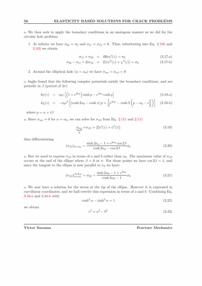
56 ELASTICITY BASED SOLUTIONS FOR CRACK PROBLEMS
20 We then seek to apply the boundary conditions in an analogous manner as we did for thecircular hole problem:
1. At infinity we have σ22 = σ0 and σ11 = σ12 = 0. Thus, substituting into Eq. 2.105 and2.105 we obtain
σ11 + σ22 = 4Reψ′(z) = σ0 (3.17-a)
σ22 − σ11 + 2iσ12 = 2[zψ′′(z) + χ′′(z)] = σ0 (3.17-b)
2. Around the elliptical hole (α = α0) we have σαα = σαβ = 0
21 Inglis found that the following complex potentials satisfy the boundary conditions, and areperiodic in β (period of 2π)
4ψ(z) = σ0c[(
1 + e2α0
)sinh p − e2α0 cosh p
](3.18-a)
4χ(z) = −σ0c2[(cosh 2α0 − cosh π) p +
1
2e2α0 − cosh 2
(p − α0 − i
π
2
)](3.18-b)
where p = α + iβ
22 Since σαα = 0 for α = α0, we can solve for σββ from Eq. 2.111 and 2.111
σαα︸︷︷︸0
+σββ = 2[ψ′(z) + ψ′(z)] (3.19)
thus differentiating
(σββ)α=α0 =sinh 2αo − 1 + e2α0 cos 2β
cosh 2αo − cos 2βσ0 (3.20)
23 But we need to express σββ in terms of a and b rather than α0. The maximum value of σββ
occurs at the end of the ellipse where β = 0 or π. For those points we have cos 2β = 1, andsince the tangent to the ellipse is now parallel to x2 we have:
(σββ)β=0,πα=α0
= σ22 =sinh 2α0 − 1 + e2α0
cosh 2α0 − 1σ0 (3.21)
24 We now have a solution for the stress at the tip of the ellipse. However it is expressed incurvilinear coordinates, and we hall rewrite this expression in terms of a and b. Combining Eq.3.16-a and 3.16-b with
cosh2 α − sinh2 α = 1 (3.22)
we obtainc2 = a2 − b2 (3.23)
Victor Saouma Fracture Mechanics

3.4 Crack, (Westergaard, 1939) 57
25 The following relations
cosh 2α0 = 2cosh2 α0 − 1 (3.24-a)
sinh 2α0 = 2 sinh α0 cosh α0 (3.24-b)
when combined with cosh α0 = ac and sinh α0 = b
c yield
sinh 2α0 =2ab
c2(3.25-a)
cosh 2α0 =a2 + b2
c2(3.25-b)
26 Finally, substituting those two equations into Eq. 3.21
(σββ)β=0,πα=α0
= σ0
(1 + 2
a
b
)(3.26)
27 We observe that for a = b, we recover the stress concentration factor of 3 of a circular hole,and that for a degenerated ellipse, i.e a crack there is an infinite stress.
28 Alternatively, let ρ be the radius of curvature of a parametric curve. From analytical geom-etry,
ρ2 =
(dx2
1 + dx22
)3(dx1d2x2 − dx2d2x1)
2 (3.27)
Using a parametric representation, we can define x1 = a cos t and x2 = b sin t; substituting intothe above equation gives:
ρ2 =1
a2b2(a2 sin2 t + b2 cos2 t)3 (3.28)
At the tip of the ellipse x2 = 0 and x1 = ±a. Thus, sin t = 0 and cos t = 1, and ρ becomesequal to ρ = b2
a . Substituting into Eq. 3.26
(σββ)β=0,πα=α0
= σ0
(1 + 2
√a
ρ
)(3.29)
From this equation, we note that the stress concentration factor is inversely proportional to theradius of curvature of an opening.
3.4 Crack, (Westergaard, 1939)
29 Just as both Kolosoff (1910) and Inglis (1913) independently solved the problem of an ellip-tical hole, there are two classical solutions for the crack problem. The first one was proposed by
Victor Saouma Fracture Mechanics

58 ELASTICITY BASED SOLUTIONS FOR CRACK PROBLEMS
σ
σ
σ
σ
x
x
0
0
0
0
1
2
2a
Figure 3.3: Crack in an Infinite Plate
Westergaard, and the later by Williams. Whereas the first one is simpler to follow, the secondhas the advantage of being extended to cracks at the interface of two different homogeneousisotropic materials and be applicable for V notches.
30 Let us consider an infinite plate subjected to uniform biaxial stress σ0 with a central crack oflength 2a, Fig. 3.3. From Inglis solution, we know that there would be a theoretically infinitestress at the tip of the crack, however neither the nature of the singularity nor the stress fieldcan be derived from it.
31 Westergaard’s solution, (Westergaard 1939b) starts by assuming Φ(z) as a harmonic function(thus satisfying Laplace’s equation ∇2 (Φ) = 0). Denoting by φ′(z) and φ′′(z) the first andsecond derivatives respectively, and φ(z) and ¯φ(z) its first and second integrals respectively ofthe function φ(z).
32 Westergaard has postulated that
Φ = Re¯φ(z) + x2Imφ(z) (3.30)
is a solution to the crack problem1. φ(z) is assumed to be analytic.
33 Let us verify that Φ satisfies the biharmonic equation. Taking the first derivatives, andrecalling from from Eq. 2.97-a that ∂
∂x1f(z) = f ′(z), we have
∂Φ
∂x1=
∂
∂x1
(Re ¯φ
)+
⎡⎢⎢⎢⎣x2
∂
∂x1Imφ(z) + Imφ(z)
∂x2
∂x1︸︷︷︸0
⎤⎥⎥⎥⎦ (3.31-a)
= Reφ(z) + x2Imφ(z) (3.31-b)
1 Note that we should not confuse the Airy stress function Φ with the complex function φ(z).
Victor Saouma Fracture Mechanics

3.4 Crack, (Westergaard, 1939) 59
σ22 =∂2Φ
∂x21
=∂
∂x1
(Reφ(z)
)+
[x2
∂
∂x1Imφ(z) + Imφ(z)
∂x2
∂x1
](3.31-c)
= Reφ(z) + x2Imφ′(z) (3.31-d)
34 Similarly, differentiating with respect to x2, and recalling from Eq. 2.97-b that ∂∂x2
f(z) =if ′(z), we obtain
∂Φ
∂x2=
∂
∂x2(Re¯φ(z) + [x2
∂
∂x2
(Imφ(z)
)+
∂x2
∂x2Imφ(z)] (3.32-a)
= −Imφ(z) + x2Reφ(z) + Imφ(z) (3.32-b)
σ11 =∂2Φ
∂x22
= x2∂
∂x2Reφ(z) + Reφ(z)
∂x2
∂x2(3.32-c)
= −x2Imφ′(z) + Reφ(z) (3.32-d)
35 Similarly, it can be shown that
σ12 = − ∂2Φ
∂x1∂x2= −x2Reφ′(z) (3.33)
36 Having derived expressions for the stresses and the second partial derivatives of Φ, substi-tuting into Eq. 2.94, it can be shown that the biharmonic equation is satisfied, thus Φ is a validsolution.
37 If we want to convince ourselves that the stresses indeed satisfy both the equilibrium andcompatibility equations (which they do by virtue of Φ satisfying the bi-harmonic equation), wehave from Eq. 2.72 in 2D:
1. Equilibrium:
∂σ11
∂x1+
∂σ12
∂x2= 0 (3.34-a)
∂σ22
∂x2+
∂σ12
∂x1= 0 (3.34-b)
Let us consider the first equation
∂σ11
∂x1=
∂
∂x1
(∂2Φ
∂x22
)=
∂
∂x1[Reφ(z) − x2Imφ′(z)] (3.35-a)
= Reφ′(z) − x2Imφ′′(z) (3.35-b)
∂σ12
∂x2=
∂
∂x2
(∂2Φ
∂x1∂x2
)=
∂
∂x2[−x2Reφ′(z)] (3.35-c)
= −Reφ′(z) + x2∂
∂x1Imφ′(z) (3.35-d)
= −Reφ′(z) + x2Imφ′′(z) (3.35-e)
Victor Saouma Fracture Mechanics

60 ELASTICITY BASED SOLUTIONS FOR CRACK PROBLEMS
If we substitute those two equations into Eq. 3.34-a then we do obtain zero. Similarly,it can be shown that Eq. 3.34-b is satisfied.
2. Compatibility: In plane strain, displacements are given by
2μu1 = (1 − 2ν)Re φ(z) − x2Imφ(z) (3.36-a)
2μu2 = 2(1 − ν)Imφ(z) − x2Re φ(z) (3.36-b)
and are obtained by integration of the strains, which in turn are obtained from thestresses. As a check we compute
2με11 =∂u1
∂x1(3.37-a)
= (1 − 2ν)Reφ(z) − x2Imφ′(z) (3.37-b)
= (1 − ν) [Reφ(z) − x2Imφ′(z)]︸ ︷︷ ︸σ11
−ν [Reφ(z) + x2Imφ′(z)]︸ ︷︷ ︸σ22
(3.37-c)
= (1 − ν)σ11 − νσ22 (3.37-d)
Recalling that
μ =E
2(1 + ν)(3.38)
thenEε11 = (1 − ν2)σ11 − ν(1 + ν)σ22 (3.39)
this shows that Eε11 = σ11 − ν(σ22 − σ33), and for plane strain, ε33 = 0 ⇒ σ33 =ν(σ11 + σ22) and Eε11 = (1 − ν2)σ11 − ν(1 + ν)σ22
38 So far Φ was defined independently of the problem, and we simply determined the stressesin terms of it, and verified that the bi-harmonic equation was satisfied.
39 Next, we must determine φ such that the boundary conditions are satisfied. For reasonswhich will become apparent later, we generalize our problem to one in which we have a biaxialstate of stress applied on the plate. Hence:
1. Along the crack: at x2 = 0 and −a < x1 < a we have σ22 = 0 (traction free crack).
2. At infinity: at x2 = ±∞, σ22 = σ0
We note from Eq. 3.31-d that at x2 = 0 σ22 reduces to
(σ22)x2=0 = Reφ(z) (3.40)
40 Furthermore, we expect σ22 → σ0 as x1 → ∞, and σ22 to be greater than σ0 when | x1−a |> ε(due to anticipated singularity predicted by Inglis), thus a possible choice for σ22 would be
Victor Saouma Fracture Mechanics

3.4 Crack, (Westergaard, 1939) 61
σ22 = σ01− a
x1
, for symmetry, this is extended to σ22 = σ0(1− a2
x21
) . However, we also need to have
σ22 = 0 when x2 = 0 and −a < x1 < a, thus the function φ(z) should become imaginary alongthe crack, and
σ22 = Re
⎛⎜⎜⎝ σ0√
1 − a2
x21
⎞⎟⎟⎠ (3.41)
41 Thus from Eq. 3.40 we have (note the transition from x1 to z).
φ(z) =σ0√
1 − a2
z2
(3.42)
42 If we perform a change of variable and define η = z − a = reiθ and assuming ηa � 1, and
recalling that eiθ = cos θ + i sin θ, then the first term of Eq. 3.31-d can be rewritten as
Reφ(z) = Reσ0√
η2+2aηη2+a2+2aη
≈ Reσ0√2aηa2
≈ Reσ0
√a
2η≈ Reσ0
√a
2reiθ≈ Reσ0
√a
2re−i θ
2 ≈ σ0
√a
2rcos
θ
2(3.43-a)
43 Recalling that sin 2θ = 2 sin θ cos θ and that e−iθ = cos θ− i sin θ, we substituting x2 = r sin θinto the second term
x2Imφ′ = r sin θImσ0
2
√a
2(reiθ)3= σ0
√a
2rsin
θ
2cos
θ
2sin
3θ
2(3.44)
44 Combining the above equations, with Eq. 3.31-d, 3.32-d, and 3.33 we obtain
σ22 = σ0
√a2r cos θ
2
(1 + sin θ
2 sin 3θ2
)+ · · ·
σ11 = σ0
√a2r cos θ
2
(1 − sin θ
2 sin 3θ2
)+ · · ·
σ12 = σ0
√a2r sin θ
2 cos θ2 cos 3θ
2 + · · ·(3.45)
45 Recall that this was the biaxial case, the uniaxial case may be reproduced by superimposinga pressure in the x1 direction equal to −σ0, however this should not affect the stress field closeto the crack tip.
46 Using a similar approach, we can derive expressions for the stress field around a crack tipin a plate subjected to far field shear stresses (mode II as defined later) using the followingexpression of φ
ΦII(z) = −x2ReφII(z) ⇒ φII =τ√
1 − a2
z2
(3.46)
Victor Saouma Fracture Mechanics
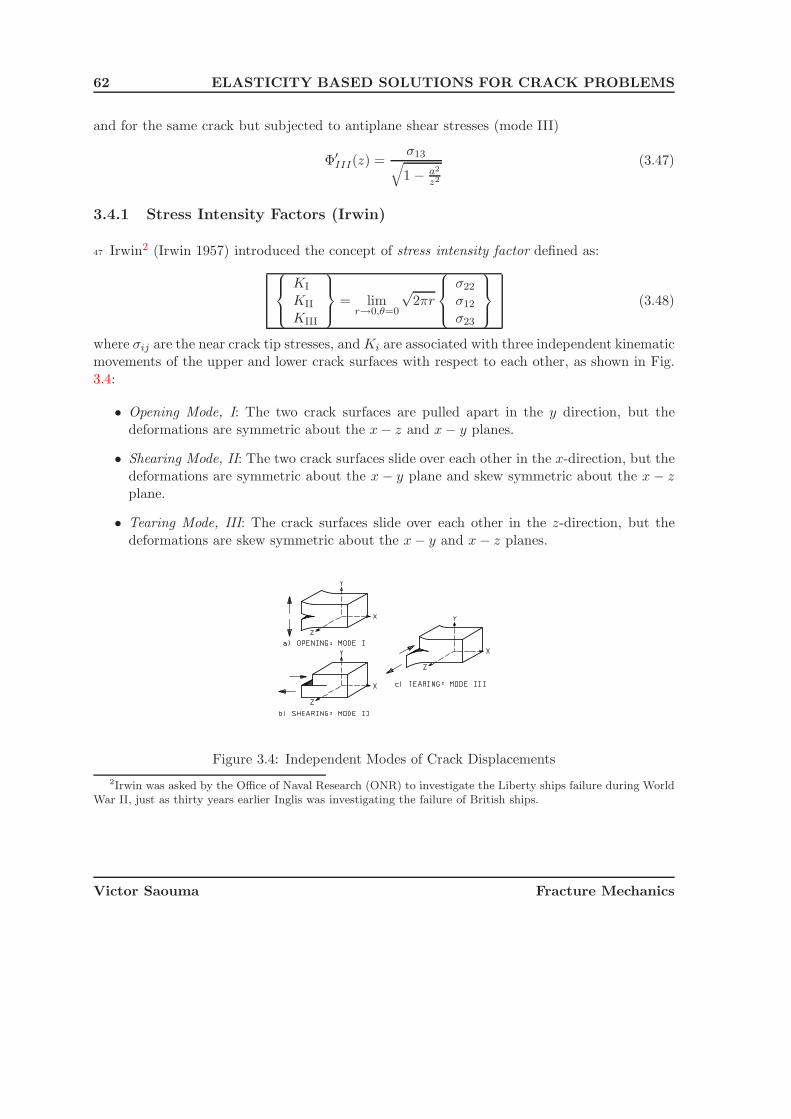
62 ELASTICITY BASED SOLUTIONS FOR CRACK PROBLEMS
and for the same crack but subjected to antiplane shear stresses (mode III)
Φ′III(z) =
σ13√1 − a2
z2
(3.47)
3.4.1 Stress Intensity Factors (Irwin)
47 Irwin2 (Irwin 1957) introduced the concept of stress intensity factor defined as:⎧⎪⎨⎪⎩
KI
KII
KIII
⎫⎪⎬⎪⎭ = lim
r→0,θ=0
√2πr
⎧⎪⎨⎪⎩
σ22
σ12
σ23
⎫⎪⎬⎪⎭ (3.48)
where σij are the near crack tip stresses, and Ki are associated with three independent kinematicmovements of the upper and lower crack surfaces with respect to each other, as shown in Fig.3.4:
• Opening Mode, I: The two crack surfaces are pulled apart in the y direction, but thedeformations are symmetric about the x − z and x − y planes.
• Shearing Mode, II: The two crack surfaces slide over each other in the x-direction, but thedeformations are symmetric about the x − y plane and skew symmetric about the x − zplane.
• Tearing Mode, III: The crack surfaces slide over each other in the z-direction, but thedeformations are skew symmetric about the x − y and x − z planes.
Figure 3.4: Independent Modes of Crack Displacements
2Irwin was asked by the Office of Naval Research (ONR) to investigate the Liberty ships failure during WorldWar II, just as thirty years earlier Inglis was investigating the failure of British ships.
Victor Saouma Fracture Mechanics

3.4 Crack, (Westergaard, 1939) 63
48 From Eq. 3.45, 3.45 and 3.45 with θ = 0, we have
KI =√
2πrσ22
=√
2πrσ0
√a
2r
= σ0√
πa (3.49-a)
where r is the length of a small vector extending directly forward from the crack tip.
49 Thus stresses and displacements can all be rewritten in terms of the SIF⎧⎪⎨⎪⎩
σ22
σ12
σ23
⎫⎪⎬⎪⎭ =
1√2πr
⎡⎢⎣ f I
11(θ) f II11 (θ) f III
11 (θ)f I22(θ) f II
22 (θ) f III22 (θ)
f I12(θ) f II
12 (θ) f III12 (θ)
⎤⎥⎦⎧⎪⎨⎪⎩
KI
KII
KIII
⎫⎪⎬⎪⎭ (3.50-a)
i.e.
σ12 =KII√2πr
sinθ
2cos
θ
2cos
3θ
2︸ ︷︷ ︸fII22
(3.51)
1. Since higher order terms in r were neglected, previous equations are exact in the limit asr → 0
2. Distribution of elastic stress field at tip can be described by KI ,KII and KIII . Note thatthis polar distribution is identical for all cases. As we shall see later, for anisotropic cases,the spatial distribution is a function of elastic constants.
3. SIF are additives, i.e.
4. The SIF is the measure of the strength of the singularity (analogous to SCF)
5. K = f(g)σ√
πa where f(g) is a parameter3 that depends on the specimen, crack geometry,and loading.
6. Tada “Stress Analysis of Cracks”, (Tada, Paris and Irwin 1973); and Cartwright & Rooke,“Compendium of Stress Intensity Factors” (Rooke and Cartwright 1976).
7. One of the underlying principles of FM is that unstable fracture occurs when the SIFreaches a critical value KIc. KIc or fracture toughness represents the inherent ability ofa material to withstand a given stress field intensity at the tip of a crack and to resistprogressive tensile crack extensions.
3Note that in certain literature, (specially the one of Lehigh University), instead of K = f(g)σ√
πa, k =f(g)σ
√a is used.
Victor Saouma Fracture Mechanics

64 ELASTICITY BASED SOLUTIONS FOR CRACK PROBLEMS
3.4.2 Near Crack Tip Stresses and Displacements in Isotropic Cracked Solids
50 Using Irwin’s concept of the stress intensity factors, which characterize the strength of thesingularity at a crack tip, the near crack tip (r � a) stresses and displacements are alwaysexpressed as:
Pure mode I loading:
σxx =KI
(2πr)12
cosθ
2
[1 − sin
θ
2sin
3θ
2
](3.52-a)
σyy =KI
(2πr)12
cosθ
2
[1 + sin
θ
2sin
3θ
2
](3.52-b)
τxy =KI
(2πr)12
sinθ
2cos
θ
2cos
3θ
2(3.52-c)
σzz = ν(σx + σy)τxz = τyz = 0 (3.52-d)
u =KI
2μ
[r
2π
] 12
cosθ
2
[κ − 1 + 2 sin2 θ
2
](3.52-e)
v =KI
2μ
[r
2π
] 12
sinθ
2
[κ + 1 − 2 cos2 θ
2
](3.52-f)
w = 0 (3.52-g)
Pure mode II loading:
σxx = − KII
(2πr)12
sinθ
2
[2 + cos
θ
2cos
3θ
2
](3.53-a)
σyy =KII
(2πr)12
sinθ
2cos
θ
2cos
3θ
2(3.53-b)
τxy =KII
(2πr)12
cosθ
2
[1 − sin
θ
2sin
3θ
2
](3.53-c)
σzz = ν(σx + σy) (3.53-d)
τxz = τyz = 0 (3.53-e)
u =KII
2μ
[r
2π
] 12
sinθ
2
[κ + 1 + 2 cos2 θ
2
](3.53-f)
v = −KII
2μ
[r
2π
] 12
cosθ
2
[κ − 1 − 2 sin2 θ
2
](3.53-g)
w = 0 (3.53-h)
Pure mode III loading:
τxz = − KIII
(2πr)12
sinθ
2(3.54-a)
Victor Saouma Fracture Mechanics

3.5 V Notch, (Williams, 1952) 65
τyz =KIII
(2πr)12
cosθ
2(3.54-b)
σxx = σy = σz = τxy = 0 (3.54-c)
w =KIII
μ
[2r
π
] 12
sinθ
2(3.54-d)
u = v = 0 (3.54-e)
where κ = 3 − 4ν for plane strain, and κ = 3−ν1+ν for plane stress.
51 Using Eq. 2.48-a, 2.48-b, and 2.48-c we can write the stresses in polar coordinates
Pure mode I loading:
σrr =KI√2πr
cosθ
2
(1 + sin2 θ
2
)(3.55-a)
σθθ =KI√2πr
cosθ
2
(1 − sin2 θ
2
)(3.55-b)
τrθ =KI√2πr
sinθ
2cos2 θ
2(3.55-c)
Pure mode II loading:
σrr =KII√2πr
(−5
4sin
θ
2+
3
4sin
3θ
2
)(3.56-a)
σθθ =KII√2πr
(−3
4sin
θ
2− 3
4sin
3θ
2
)(3.56-b)
τrθ =KII√2πr
(1
4cos
θ
2+
3
4cos
3θ
2
)(3.56-c)
3.5 V Notch, (Williams, 1952)
52 Using the method of separation of variables in 1952, Williams (Williams 1952, Williams 1957)proposed the following solution
Φ(r, θ) ≡ rλ+1F (θ, λ) (3.57)
where F (θ, λ) = em(λ)θ , and m(λ) is yet to be determined, by satisfying the bi-harmonicequation, Eq. 2.95
∇2(∇2Φ
)=
(∂2
∂r2+
1
r
∂
∂r+
1
r2
∂2
∂θ2
)(∂2Φ
∂r2+
1
r
∂Φ
∂r+
1
r2
∂2Φ
∂θ2
)= 0 (3.58)
Victor Saouma Fracture Mechanics

66 ELASTICITY BASED SOLUTIONS FOR CRACK PROBLEMS
2
r
γ
θ
α
P
Figure 3.5: Plate with Angular Corners
53 Note that the problem he originally considered was not a crack, but rather a plate undertension with angular corners, Fig. 3.5 making an angle 2γ. For γ = 0 we recover the crackproblem of Westergaard.
54 Substituting Eq. 3.57 into the biharmonic equation (Eq. 3.58) gives
∂4F (θ, λ)
∂θ4+ 2(λ2 + 1)
∂2F (θ, λ)
∂θ2+ (λ2 − 1)2F (θ, λ) = 0 (3.59)
55 Substituting F (θ, λ) with em(λ)θ , this equation reduces to
em(λ)θ[(λ − 1)2 + m(λ)2
] [(1 + λ)2 + m(λ)2
]= 0 (3.60)
56 The roots of this equation are
m(λ) = ±i (λ − 1) (3.61-a)
m(λ) = ±i (λ + 1) (3.61-b)
57 Since F (θ, λ) is a real function then the solutions of the differential equation 3.58 are alsoreal functions. Recalling that
eim(λ)θ = cos m(λ)θ + i sin m(λ)θ (3.62)
we select as solutionF1(θ, λ) = cos(λ − 1)θF2(θ, λ) = cos(λ + 1)θF3(θ, λ) = sin(λ − 1)θF4(θ, λ) = sin(λ + 1)θ
(3.63)
Victor Saouma Fracture Mechanics

3.5 V Notch, (Williams, 1952) 67
and finally F (θ, λ) will be a linear combination of F1, F2, F3 and F4, thus
Φ(r, θ) = rλ+1 [A cos(λ − 1)θ + B cos(λ + 1)θ + C sin(λ − 1)θ + D sin(λ + 1)θ]︸ ︷︷ ︸F (θ,λ)
(3.64)
58 Next, we seek to determine the stresses in polar coordinates in order to apply the boundaryconditions. Substituting Eq. 3.57 into Eq. 2.93
σθθ =∂2Φ
∂r2(3.65-a)
σrθ = − ∂
∂r
(1
r
∂Φ
∂θ
)(3.65-b)
we obtain:
σθθ = rλ−1λ(λ + 1)F (θ) (3.66-a)
σrθ = rλ−1[−λF ′(θ)] (3.66-b)
Substituting
σθθ = rλ−1λ(λ + 1)[A cos(λ − 1)θ + B cos(λ + 1)θ
+ C sin(λ − 1)θ + D sin(λ + 1)θ] (3.67-a)
σrθ = −λrλ−1[−A(λ − 1) sin(λ − 1)θ − B(λ + 1) sin(λ + 1)θ
+ C(λ − 1) cos(λ − 1)θ + D(λ + 1) cos(λ + 1)θ] (3.67-b)
59 The boundary conditions are next applied by considering a plate with a central crack, ap-plying the following 4 boundary conditions along the crack edges
σθθ |θ=±α = 0 (3.68-a)
σrθ |θ=±α = 0 (3.68-b)
where α + γ = π, which implies that
F (α) = F (−α) = F ′(α) = F ′(−α) = 0 (3.69)⎡⎢⎢⎢⎣
cos(λ − 1)α cos(λ + 1)α 0 0ω sin(λ − 1)α sin(λ + 1)α 0 0
0 0 sin(λ − 1)α sin(λ + 1)α0 0 ω cos(λ − 1)α cos(λ + 1)α
⎤⎥⎥⎥⎦⎧⎪⎪⎪⎨⎪⎪⎪⎩
ABCD
⎫⎪⎪⎪⎬⎪⎪⎪⎭ = 0 (3.70)
where ω = λ−1λ+1 .
60 Note that whereas Eq. 3.66-a and 3.66-b are expressed in terms of the four constants (A,B,C,and D), the above equation is written in terms of the summation and the differences of thestress equations, thus yielding a block diagonal matrix.
Victor Saouma Fracture Mechanics

68 ELASTICITY BASED SOLUTIONS FOR CRACK PROBLEMS
61 It can readily be seen that A and B are independent of C and D, and that for this homoge-neous equation a nontrivial solution would exist if and only if the determinant of the system oflinear equations vanishes to zero. This would lead (after some simplifications) to:
sin 2λα ± λ sin 2α = 0 (3.71)
62 We observe from Eq. 3.64 that the coefficients A and B correspond to symmetric loadings(mode I), and C and D to unsymmetric loading (mode II).
63 Let us denote by λn the eigenvalues of λ which are solution of Eq. 3.71 for the symmetricalloading, and ξn solutions for the antisymmetric loading:
sin 2λnα + λn sin 2α = 0 (3.72-a)
sin 2ξnα − ξn sin 2α = 0 (3.72-b)
64 For the case of a crack, i.e α = π solution of the characteristic equation4 is
sin(2πλn) = 0 (3.73-a)
sin(2πξn) = 0 (3.73-b)
which has solutions λn = n2 with n = 1, 3, 4, · · · (it can be shown that n = 2 gives rise to a
rigid body motion contribution). Substituting into Eq. 3.64
F (θ, λ) = An cos
(n
2− 1
)θ + Bn cos
(n
2+ 1
)θ
+Cn sin
(n
2− 1
)θ + Dn sin
(n
2+ 1
)θ (3.74-a)
65 We observe that the previous expression can be simplified by noting that for each eigenvalueλn and ξn there is a relationship between A and B, and between C and D in Eq. 3.70. Forsymmetrical loading we have
An cos(λn − 1)α + Bn cos(λn + 1)α = 0 (3.75-a)
Anω sin(λn − 1)α + Bn sin(λn + 1)α = 0 (3.75-b)
and for antisymmetric loading we have
Cn sin(ξn − 1)α + Dn sin(ξn + 1)α = 0 (3.76-a)
Cnω cos(ξn − 1)α + Dn cos(ξn + 1)α = 0 (3.76-b)
4Note that the solution for λn and ξn for other angles can not be obtained algebraically, a numerical techniquemust be used.
Victor Saouma Fracture Mechanics
3.5 V Notch, (Williams, 1952) 69
66 Thus we can define
an =An
Bn= −cos(λn − 1)α
cos(λn + 1)α= −ω sin(λn − 1)α
sin(λn + 1)α(3.77-a)
bn =Cn
Dn= −sin(λn − 1)α
sin(λn + 1)α= −ω cos(λn − 1)α
cos(λn + 1)α(3.77-b)
these ratios are equal to 1/3 and −1 respectively for α = π and λ = 1/2. and
F (θ) =∑[
an
(sin
3
2θ + sin
1
2θ
)+ bn
(1
3cos
3
2θ + cos
1
2θ
)](3.78)
67 The stresses are obtained by substituting
σrr =∑[
bn√r
(5
4cos
θ
2− 1
4cos
3θ
2
)+
an√r
(−5
4sin
θ
2+
3
4sin
3θ
2
)](3.79-a)
σθθ =∑[
bn√r
(3
4cos
θ
2+
1
4cos
3θ
2
)+
an√r
(−3
4sin
θ
2− 3
4sin
3θ
2
)](3.79-b)
σrθ =∑[
bn√r
(1
4sin
θ
2+
1
4sin
3θ
2
)+
an√r
(1
4cos
θ
2+
3
4cos
3θ
2
)](3.79-c)
68 These equations can be further simplified into
σrr =∑[
bn√r
cosθ
2
(1 + sin2 θ
2
)+
an√r
(−5
4sin
θ
2+
3
4sin
3θ
2
)](3.80-a)
σθθ =∑[
bn√r
cosθ
2
(1 − sin2 θ
2
)+
an√r
(−3
4sin
θ
2− 3
4sin
3θ
2
)](3.80-b)
σrθ =∑[
bn√r
sinθ
2cos2 θ
2+
an√r
(1
4cos
θ
2+
3
4cos
3θ
2
)](3.80-c)
69 Finally, it can be shown that the displacements will be given by
u =1
2μ
∑Re{anrλn [(κ + λn cos 2α + cos 2λnα) cos λnθ − λn cos(λn − 2)θ]
−bnrξn [(κ + ξn cos 2α − cos 2ξnα) sin ξnθ − ξn sin(ξn − 2)θ]}
(3.81-a)
v =1
2μ
∑Re{anrλn [(κ − λn cos 2α − cos 2λnα) sin λnθ + λn sin(λn − 2)θ]
+bnrξn [(κ − ξn cos 2α + cos 2ξnα) cos ξnθ + ξn cos(ξn − 2)θ]}
(3.81-b)
Victor Saouma Fracture Mechanics

70 ELASTICITY BASED SOLUTIONS FOR CRACK PROBLEMS
Ε ,
Ε ,
ν
ν
1 1
2 2
Figure 3.6: Plate with Angular Corners
70 This solution can be compared with Westergaard’s solution by comparing Equations 3.55-aand 3.56-a with Eq. 3.80-a; Eq. 3.55-b and 3.56-b with Eq. 3.80-b; and Eq. 3.55-c and 3.56-cwith Eq. 3.80-c for n = 1. From this we observe that
b1 = KI√2π
a1 = KII√2π
(3.82)
3.6 Crack at an Interface between Two Dissimilar Materials
(Williams, 1959)
3.6.1 General Function
71 We shall now consider the problem of a crack at the interface between two dissimilar isotropicmaterials, (Williams 1959, Zak and Williams 1963). Accordingly, we rewrite Eq. 3.57 as
Φi(r, θ) ≡ rλ+1Fi(θ, λ) (3.83)
where the subscript i refers to material 1 and 2, Fig. 3.6
72 Hence:
Fi(θ, λ) = Ai cos(λ − 1)θ + Bi cos(λ + 1)θ + Ci sin(λ − 1)θ + Di sin(λ + 1)θ (3.84)
3.6.2 Boundary Conditions
73 Boundary conditions for this problem are:
Victor Saouma Fracture Mechanics

3.6 Crack at an Interface between Two Dissimilar Materials (Williams, 1959) 71
• zero stresses, σθθ, on the free edges (at θ = ±π). Thus from Eq. 3.66-a
σθθ|θ=π = rλ−1λ(λ + 1)[A1 cos(λ − 1)π + B1 cos(λ + 1)π
+C1 sin(λ − 1)π + D1 sin(λ + 1)π] = 0 (3.85-a)
σθθ|θ=−π = rλ−1λ(λ + 1)[A2 cos(λ − 1)π + B2 cos(λ + 1)π
−C2 sin(λ − 1)π − D2 sin(λ + 1)π] = 0 (3.85-b)
or F1(π) = F2(−π) = 0
• zero stresses, σrθ, on the free edges (at θ = ±π); From Eq. 3.66-b
σrθ|θ=π = −λrλ−1[−A1(λ − 1) sin(λ − 1)θ − B1(λ + 1) sin(λ + 1)θ
+C1(λ − 1) cos(λ − 1)θ + D1(λ + 1) cos(λ + 1)θ] = 0 (3.86-a)
σrθ|θ=−π = −λrλ−1F ′(θ) (3.86-b)
= −λrλ−1[+A2(λ − 1) sin(λ − 1)θ + B2(λ + 1) sin(λ + 1)θ
−C2(λ − 1) cos(λ − 1)θ − D2(λ + 1) cos(λ + 1)θ] = 0 (3.86-c)
or F ′1(π) = F ′
2(−π) = 0
• Continuity of σθθ at the interface, θ = 0
A1 + B1 = A2 + B2 (3.87)
• Continuity of σrθ at θ = 0 along the interface
(λ − 1)C1 + (λ + 1)D1 = −(λ − 1)C2 − (λ + 1)D2 (3.88)
• Continuity of displacements (ur, uθ) at the interface. Using the polar expression of thedisplacements
uir =
1
2μirλ{−(λ + 1)Fi(θ) + 4(1 − αi)[Ci sin(λ − 1)θ + Ai cos(λ − 1)θ]}(3.89-a)
uiθ =
1
2μirλ{−F ′
i (θ) − 4(1 − αi)[Ci cos(λ − 1)θ − Ai sin(λ − 1)θ]} (3.89-b)
where μ is the shear modulus, and αi ≡ νi
1+νi
we obtain
1
2μ1[−(λ + 1)F1(0) + 4A1(1 − α1)] =
1
2μ2[−(λ + 1)F2(0) + 4A2(1 − α2)](3.90-a)
1
2μ1
[−F ′1(0) − 4C1(1 − α1)
]=
1
2μ2
[−F ′2(0) − 4C2(1 − α2)
](3.90-b)
Victor Saouma Fracture Mechanics

72 ELASTICITY BASED SOLUTIONS FOR CRACK PROBLEMS
3.6.3 Homogeneous Equations
74 Applying those boundary conditions, will lead to 8 homogeneous linear equations (Eq. 3.85-a,3.85-b, 3.86-b, 3.86-c, 3.87, 3.88, 3.90-a, 3.90-b) in terms of the 8 unknowns A1, B1, C1,D1, A2, B2, C2
and D2.
75 A nontrivial solution exists if the determinant of the 8 equations is equal to zero. Thisdeterminant5 is equal to
cot2 λπ +
[2k(1 − α2) − 2(1 − α1) − (k − 1)
2k(1 − α2) + 2(1 − α1)
]2= 0 (3.91)
where k = μ1
μ2.
76 For the homogeneous case α1 = α2 and k = 1, the previous equation reduces to cot2 λπ = 0or sin2 λπ = 0 thus we recover the same solution as the one of Eq. 3.73-b for a crack in onematerial:
λ =n
2n = 1, 2, 3, ... (3.92)
Note that we exclude negative values of n to ensure finite displacements as the origin is ap-proached, and the lowest eigenvalue controls.
77 Noting that there can not be a real solution to Eq. 3.91, we define
β =2k(1 − α2) − 2(1 − α1) − (k − 1)
2k(1 − α2) + 2(1 − α1)(3.93)
and thus, Eq. 3.91 leads to cot2 λπ = −β2, or
cot λπ = ±iβ (3.94)
78 To solve this equation, we use the following trigonometric relations, (Abramowitz and Stegun1970)
cot z =sin 2x − i sinh 2y
cosh 2y − cos 2x(3.95-a)
sin 2θπ =2u
1 + u2(3.95-b)
cos 2θπ =1 − u2
1 + u2(3.95-c)
sinh 2θπ =2v
1 − v2(3.95-d)
cosh 2θπ =1 + v2
1 − v2(3.95-e)
5The original paper states: ... After some algebraic simplification...
Victor Saouma Fracture Mechanics

3.6 Crack at an Interface between Two Dissimilar Materials (Williams, 1959) 73
where
u = tan λrπ (3.96-a)
v = tanh λjπ (3.96-b)
where we have assumed a complex value for λ
λ = λr + iλj (3.97)
Then, we obtain
sin 2λrπ =2u
1 + u2(3.98-a)
cos 2λrπ =1 − u2
1 + u2(3.98-b)
sinh 2λjπ =2v
1 − v2(3.98-c)
cosh 2λjπ =1 + v2
1 − v2(3.98-d)
79 Substituting in Eq. 3.95-a lead to
cot λπ =u(1 − v2) − iv(1 + u2)
u2 + v2(3.99-a)
=tan λrπ(1 − tanh2 λjπ)
tan2 λrπ + tanh2 λjπ︸ ︷︷ ︸Re(cot λπ)=0
−i(tan2 λrπ + 1) tanh λjπ
tan2 λrπ + tanh2 λjπ︸ ︷︷ ︸Im(cot λπ)=±β
(3.99-b)
80 Thus, Eq. 3.91 finally leads to
Re(cot λπ) = 0 (3.100-a)
Im(cot λπ) = ±β (3.100-b)
we thus have two equations with two unknowns.
3.6.4 Solve for λ
81 Let us solve those two equations. Two sets of solutions are possible:
1. If from 3.99-b tan λrπ = 0 then
λr = n = 0, 1, 2, 3, ... (3.101)
and accordingly from Eq. 3.100-b
λj = ± 1
πcoth−1 β (3.102)
Victor Saouma Fracture Mechanics

74 ELASTICITY BASED SOLUTIONS FOR CRACK PROBLEMS
2. Alternatively, from Eq. 3.100-a cot λrπ = 0 ⇒ tan λrπ = ∞ and6:
λr =2n + 1
2n = 0, 1, 2, 3, ... (3.103-a)
λj = ± 1
πtanh−1 β (3.103-b)
=1
2πlog
[β + 1
β − 1
](3.103-c)
We note that for this case, λj → 0 as α1 → α2 and k → 1 in β.
3.6.5 Near Crack Tip Stresses
82 Now that we have solved for λ, we need to derive expressions for the near crack tip stressfield. We rewrite Eq. 3.83 as
Φ(r) = rλ+1︸ ︷︷ ︸G(r)
F (θ, λ) (3.104)
we note that we no longer have two sets of functions, as the effect of dissimilar materials hasbeen accounted for and is embedded in λ.
83 The stresses will be given by Eq. 2.93
σrr =1
r2
∂2Φ
∂θ2+
1
r
∂Φ
∂r= r−2G(r)F ′′(θ) + r−1G′(r)F (θ) (3.105-a)
σθθ =∂2Φ
∂r2= G′′(r)F (θ) (3.105-b)
σrθ =1
r2
∂Φ
∂θ− 1
r
∂2Φ
∂r∂θ= r−2G(r)F ′(θ) − r−1G′(r)F ′(θ) (3.105-c)
Therefore, we must solve for F ′(θ), F ′′(θ), G′(r) and G′′(r) in terms of λ = λr + iλj.
84 First we note that
G(r) = rλ+1 = rλr+1+iλj (3.106-a)
riλj = eiλj log(r) (3.106-b)
recalling that log(z) = log |z| + i arg z, and since |z| =√
x2 + y2 =√
r2 + 0 = r, we havearg z = 2kπ, and k = 0,±1,±2, · · ·. Hence,
log(r) = log |r| + i2kπ (3.107)
and Eq. 3.106-b becomes
riλj = eiλj log(r) (3.108-a)
6Recall that tanh−1 x = 12
log 1+x1−x
Victor Saouma Fracture Mechanics

3.6 Crack at an Interface between Two Dissimilar Materials (Williams, 1959) 75
= eiλj [log(r)+i2kπ (3.108-b)
= eiλj log(r)−2kπλj (3.108-c)
= e−2kπλjeiλj log(r) (3.108-d)
= e−2kπλj [cos (λj log(r)) + i sin (λj log(r))] (3.108-e)
85 Now, for k = 0, riλj becomes
riλj = cos(λj log(r)) + i sin(λj log(r)) (3.109)
and accordingly, Eq. 3.106-a becomes
G(r) = rλ+1 = rλr+1riλj (3.110-a)
= rλr+1 [cos(λj log(r)) + i sin(λj log(r))] (3.110-b)
and for λr = 1/2
G(r) = r32 [cos(λj log(r)) + i sin(λj log(r))] (3.111-a)
ReG(r) = r32 cos(λj log(r)) (3.111-b)
G′(r) = r12
[3
2cos(λj log(r)) + λj sin(λj log(r))
](3.111-c)
G′′(r) = r−12
[(3
4− λ2
j
)cos(λj log(r)) +
(3
2+
λj
2
)sin(λj log(r))
](3.111-d)
86 Back to F (θ), which was defined in Eq. 3.84
F (θ, λ) = A cos(λ − 1)θ + B cos(λ + 1)θ + C sin(λ − 1)θ + D sin(λ + 1)θ (3.112)
we need to replace λ by λr + iλj . However, first we recall the following relations, (Abramowitzand Stegun 1970)
sin(x + iy) = sin(x) cosh(y) − i cos(x) sinh(y) (3.113-a)
cos(x + iy) = cos(x) cosh(y) + i sin(x) sinh(y) (3.113-b)
thus,
Re {sin [(λr ± 1) + iλj ] θ} = sin(λr ± 1) cos(θ) cosh λjθ (3.114-a)
Re {cos [(λr ± 1) + iλj ] θ} = cos(λr ± 1) cos(θ) cosh λjθ (3.114-b)
Victor Saouma Fracture Mechanics

76 ELASTICITY BASED SOLUTIONS FOR CRACK PROBLEMS
87 Substituting those relations in Eq. 3.112
Re [F (θ)] = cosh λjθ︸ ︷︷ ︸f(θ)
(3.115-a)
[A cos(λr − 1)θ + B cos(λr + 1)θ + C sin(λr − 1)θ + D sin(λr + 1)θ]︸ ︷︷ ︸g(θ)
(3.115-b)
Re [Φ(r, θ)] = rλr+1 cos(λj log(r)) cosh λjθ
[A cos(λr − 1)θ + B cos(λr + 1)θ
+C sin(λr − 1)θ + D sin(λr + 1)θ] (3.115-c)
88 For λr = 12
g(θ) = A cosθ
2+ B cos
3θ
2− C sin
θ
2+ D sin
3θ
2(3.116)
89 Applying the boundary conditions at θ = ±π, σθθ = 0, Eq. 3.105-b F (θ) = 0, that isg1(−π) = g2(π) or
C = −D = −a (3.117)
90 Similarly at θ = ±π, σrθ = 0. Thus, from Eq. 3.105-c F ′(θ) = 0, or g′1(−π) = g′2(π) or
A = 3B = b (3.118)
91 From those two equations we rewrite Eq. 3.116
g(θ) = a
(sin
θ
2+ sin
3θ
2
)+ b
(3 cos
θ
2+ cos
3θ
2
)(3.119)
92 We now determine the derivatives
f ′(θ) = λj sinhλjθ (3.120-a)
g′(θ) = a
(3
2cos
3θ
2+
1
2cos
θ
2
)+ b
(−3
2sin
3θ
2− 3
2sin
θ
2
)(3.120-b)
93 Thus, we now can determine
F ′(θ) = f ′(θ)g(θ) + f(θ)g′(θ) (3.121-a)
= a
{cosh λjθ
[3
2cos
3θ
2+
1
2cos
θ
2
]+ λj sinhλjθ
[sin
3θ
2+ sin
θ
2
]}
+b
{cosh λjθ
[−3
2sin
3θ
2− 3
2sin
θ
2
]+ λj sinhλjθ
[cos
3θ
2+ 3 cos
θ
2
]}(3.121-b)
Victor Saouma Fracture Mechanics

3.7 Homogeneous Anisotropic Material (Sih and Paris) 77
94 Similarly, the second derivative F ′′(θ) is determined
F ′′(θ) = f ′′(θ)g(θ) + 2f ′(θ)g′(θ) + f(θ)g′′(θ) (3.122-a)
= a
{cosh λjθ
[−9
4sin
3θ
2− 1
4sin
θ
2
]+ 2λj sinhλjθ
[3
2cos
3θ
2+
1
2cos
θ
2
]
+λ2j cosh2 λjθ
[sin
3θ
2+ sin
θ
2
]}+
b
{cosh λjθ
[−9
4cos
3θ
2− 3
4cos
θ
2
]+ 2λj sinhλjθ
[−3
2sin
3θ
2− 3
2sin
θ
2
]
+λ2j cosh2 λjθ
[cos
3θ
2+ 3 cos
θ
2
]}(3.122-b)
95 We can now substitute in Eq. 3.105-b, 3.105-c and 3.105-a to determine the stresses
σrr = r−12 cos(λj log(r))F ′′(θ) + r−
12
[3
2cos(λj log(r)) + λj sin(λj log(r))
]F (θ)(3.123-a)
σθθ = r−12
[(3
4− λ2
j
)cos(λj log(r)) +
(3
2+
λj
2
)sin(λj log(r))
]F (θ) (3.123-b)
σrθ = r−12
{cos(λj log(r))F ′(θ) +
[3
2cos(λj log(r)) + λj sin(λj log(r))
]F ′(θ)
}(3.123-c)
3.7 Homogeneous Anisotropic Material (Sih and Paris)
96 To analyze an anisotropic body with with a crack, we need to derive the two stress functionsΦ1 and Φ2 in Eq. 2.122 such that they satisfy the boundary conditions of the problem underconsideration.
97 For an infinite plate with a central crack in an anisotropic body the derivation for the stressfunctions was undertaken by Sih, Paris and Irwin, (Sih, Paris and Irwin 1965). This solutionis the “counterpart” or generalization of Westergaard’s solutions.
u1 = KI
√2r
πRe
{1
s1 − s2
[s1p2 (cos θ + s2 sin θ)
12 − s2p1 (cos θ + s1 sin θ)
12
]}(3.124-a)
v1 = KI
√2r
πRe
{1
s1 − s2
[s1q2 (cos θ + s2 sin θ)
12 − s2q1 (cos θ + s1 sin θ)
12
]}(3.124-b)
w1 = 0 (3.124-c)
u2 = KII
√2r
πRe
{1
s1 − s2
[p2 (cos θ + s2 sin θ)
12 − p1 (cos θ + s1 sin θ)
12
]}(3.124-d)
Victor Saouma Fracture Mechanics

78 ELASTICITY BASED SOLUTIONS FOR CRACK PROBLEMS
v2 = KII
√2r
πRe
{1
s1 − s2
[q2 (cos θ + s2 sin θ)
12 − q1 (cos θ + s1 sin θ)
12
]}(3.124-e)
w2 = 0 (3.124-f)
u3 = 0 (3.124-g)
v3 = 0 (3.124-h)
w3 = KIII
√2r
π
(c44c55 − c2
45
)− 12Im[(cos θ + s3 sin θ)
12
](3.124-i)
98 where s1 and s2 are roots, in general complex, of Eq. 2.125 where sj = αj + iβj for j = 1, 2,and the roots of interests are taken such that βj > 0, and
pj = a11s2j + a12 − a16sj (3.125)
qj = a12sj +a22
sj− a26 (3.126)
99 After appropriate substitution, it can be shown that the cartesian stresses at the tip of thecrack for symmetric loading are
σx =KI√2πr
Re
[s1s2
s1 − s2
(s2
(cos θ + s2 sin θ)12
− s1
(cos θ + s1 sin θ)12
)](3.127-a)
σy =KI√2πr
Re
[1
s1 − s2
(s1
(cos θ + s2 sin θ)12
− s2
(cos θ + s1 sin θ)12
)](3.127-b)
σxy =KI√2πr
Re
[s1s2
s1 − s2
(1
(cos θ + s1 sin θ)12
− s1
(cos θ + s2 sin θ)12
)](3.127-c)
100 and, for plane skew-symmetric loading:
σx =KII√2πr
Re
[1
s1 − s2
(s22
(cos θ + s2 sin θ)12
− s21
(cos θ + s1 sin θ)12
)](3.128-a)
σy =KII√2πr
Re
[1
s1 − s2
(1
(cos θ + s2 sin θ)12
− 1
(cos θ + s1 sin θ)12
)](3.128-b)
σxy =KII√2πr
Re
[1
s1 − s2
(s1
(cos θ + s1 sin θ)12
− s2
(cos θ + s2 sin θ)12
)](3.128-c)
101 For in-plane loadings, these stresses can be summed to give the stresses at a distance r andan angle θ from the crack tip.
102 An important observation to be made is that the form of the stress singularity r−1/2 isidentical to the one found in isotropic solids.
Victor Saouma Fracture Mechanics

3.8 Assignment 79
103 It should be noted that contrarily to the isotropic case where both the stress magnitude andits spatial distribution are controlled by the stress intensity factor only, in the anisotropic casethey will also depend on the material elastic properties and the orientation of the crack withrespect to the principal planes of elastic symmetry (through s1 and s2).
3.8 Assignment
CVEN-6831
FRACTURE MECHANICS
Spring 2000
Victor E. Saouma
Home-Work No. 1Derivation of SIF
Due Date: Feb. 15, 2000
1. A cylindrical pressure vessel of radius R and thickness t contains a through crack of lenght2a oriented at an angle β with the circumferential direction. When the vessel is subjectedto an internal pressure p, determine the stress intensity factors at the crack tip.
σz
σz σz
σθ
σθ
σθ
R
t2a
β
2. The stress function for a crack subjected to splitting forces P, as shown below
Victor Saouma Fracture Mechanics

80 ELASTICITY BASED SOLUTIONS FOR CRACK PROBLEMS
x
2a
P
P
a
x 2
1
is given by:
φ =Pa
πz√
z2 − a2(3.129)
where z = x1 + ix2 and P is a load per unit thickness. Calculate the expressions of σ22
at x2 = 0 and derive an expression for KI . (KP = P√πa
)
Hint:
(a) At crack tip ηa << 1.
(b) η = z − a = z = reiθ
3. The stress intensity factor of the following problem:
x
x 2
1
a
P
P
B A
a
x
is given by:
KA =P√πa
√a + x
a − x(3.130)
Kb =P√πa
√a − x
a + x(3.131)
Victor Saouma Fracture Mechanics

3.8 Assignment 81
Based on those expressions, and results from the previous problem, determine the stressfunction Φ.
4. Barenblatt’s model assumes a linearly varying closing pressure at the tip of a crack,
c c2(a - c)
σ σy y
Using Mathematica and the expressions of KA and KB from the previous problem, de-termine an expression for the stress intensity factors for this case.
5. Using Mathematica, program either:
(a) Westergaard’s solution for a crack subjected to mode I and mode II loading.
(b) Williams solution for a crack along dissimilar materials.
Victor Saouma Fracture Mechanics

82 ELASTICITY BASED SOLUTIONS FOR CRACK PROBLEMS
Victor Saouma Fracture Mechanics

Chapter 4
LEFM DESIGN EXAMPLES
1 Following the detailed coverage of the derivation of the linear elastic stress field around a cracktip, and the introduction of the concept of a stress intensity factor in the preceding chapter, wenow seek to apply those equations to some (pure mode I) practical design problems.
2 First we shall examine how is linear elastic fracture mechanics (LEFM) effectively used indesign examples, then we shall give analytical solutions to some simple commonly used testgeometries, followed by a tabulation of fracture toughness of commonly used engineering ma-terials. Finally, this chapter will conclude with some simple design/analysis examples.
4.1 Design Philosophy Based on Linear Elastic Fracture Me-chanics
3 One of the underlying principles of fracture mechanics is that unstable fracture occurs whenthe stress intensity factor (SIF) reaches a critical value KIc, also called fracture toughness. KIc
represents the inherent ability of a material to withstand a given stress field intensity at the tipof a crack and to resist progressive tensile crack extension.
4 Thus a crack will propagate (under pure mode I), whenever the stress intensity factor KI
(which characterizes the strength of the singularity for a given problem) reaches a materialconstant KIc. Hence, under the assumptions of linear elastic fracture mechanics (LEFM), atthe point of incipient crack growth:
KIc = βσ√
πa (4.1)
5 Thus for the design of a cracked, or potentially cracked, structure, the engineer would haveto decide what design variables can be selected, as only, two of these variables can be fixed,and the third must be determined. The design variables are:
Material properties: (such as special steel to resist corrosive liquid) ⇒ Kc is fixed.
84 LEFM DESIGN EXAMPLES
Design stress level: (which may be governed by weight considerations) ⇒ σ is fixed.
Flaw size: 1, a.
6 In assessing the safety of a cracked body, it is essential that the crack length a be properlyknown. In most cases it is not. Thus assumptions must be made for its value, and thoseassumptions are dependent upon the crack detection methodology adopted. The presenceof a crack, equal to the smallest one that can be detected, must be assumed.
7 Thus, a simpler inspection procedure would result in a larger minimum crack size thanone detected by expensive nondestructive techniques. In return, simplified inspectionwould result in larger crack size assumptions.
Once two parameters are specified, the third one is fixed. Finally, it should be mentioned thatwhereas in most cases the geometry is fixed (hence β), occasionally, there is the possibility toalter it in such a way to reduce (or maximize) β.
4.2 Stress Intensity Factors
6 As shown in the preceding chapter, analytic derivation of the stress intensity factors of eventhe simplest problem can be quite challenging. This explain the interest developed by somemathematician in solving fracture related problems. Fortunately, a number of simple problemshave been solved and their analytic solution is found in stress intensity factor handbooks. Themost commonly referenced ones are Tada, Paris and Irwin’s (Tada et al. 1973), and Roorke andCartwright, (Rooke and Cartwright 1976), and Murakami (Murakami 1987)
7 In addition, increasingly computer software with pre-programmed analytical solutions arebecoming available, specially in conjunction with fatigue life predictions.
8 Because of their importance, expressions of SIF of commonly encountered geometries will belisted below:
Middle Tension Panel (MT), Fig. 4.1
KI =
√sec
πa
W︸ ︷︷ ︸β
σ√
πa (4.2)
=
[1 + 0.256
(a
W
)− 1.152
(a
W
)2
+ 12.2
(a
W
)3]
︸ ︷︷ ︸β
σ√
πa (4.3)
We note that for W very large with respect to a,√
π sec πaW = 1 as anticipated.
Single Edge Notch Tension Panel (SENT) for LW = 2, Fig. 4.2
1In most cases, a refers to half the total crack length.
Victor Saouma Fracture Mechanics

4.2 Stress Intensity Factors 85
Figure 4.1: Middle Tension Panel
Figure 4.2: Single Edge Notch Tension Panel
KI =
[1.12 − 0.23
(a
W
)+ 10.56
(a
W
)2
− 21.74
(a
W
)3
+ 30.42
(a
W
)4]
︸ ︷︷ ︸β
σ√
πa (4.4)
We observe that here the β factor for small crack ( aW � 1) is grater than one and is
approximately 1.12.
Double Edge Notch Tension Panel (DENT), Fig. 4.3
KI =
[1.12 + 0.43
(a
W
)− 4.79
(a
W
)2
+ 15.46
(a
W
)3]
︸ ︷︷ ︸β
σ√
πa (4.5)
Three Point Bend (TPB), Fig. 4.4
Figure 4.3: Double Edge Notch Tension Panel
Victor Saouma Fracture Mechanics

86 LEFM DESIGN EXAMPLES
Figure 4.4: Three Point Bend Beam
KI =3√
aW
[1.99 − ( a
W
) (1 − a
W
) (2.15 − 3.93 a
W + 2.7( a
W
)2)]2(1 + 2 a
W
) (1 − a
W
) 32
PS
BW32
(4.6)
Compact Tension Specimen (CTS), Fig. 4.5 used in ASTM E-399 (399 n.d.) StandardTest Method for Plane-Strain Fracture Toughness of Metallic Materials
KI =
[16.7 − 104.6
(a
W
)+ 370
(a
W
)2
− 574
(a
W
)3
+ 361
(a
W
)4]
︸ ︷︷ ︸β
P
BW︸ ︷︷ ︸σ
√πa (4.7)
We note that this is not exactly the equation found in the ASTM standard, but ratheran equivalent one written in the standard form.
Circular Holes: First let us consider the approximate solution of this problem, Fig. 4.6, thenwe will present the exact one:
Approximate: For a plate with a far field uniform stress σ, we know that there is astress concentration factor of 3. for a crack radiating from this hole, we consider twocases
Short Crack: aD → 0, and thus we have an approximate far field stress of 3σ, and
for an edge crack β = 1.12, Fig. 4.6 thus
KI = 1.12(3σ)√
πa
= 3.36σ√
πa (4.8)
Victor Saouma Fracture Mechanics

4.2 Stress Intensity Factors 87
Figure 4.5: Compact Tension Specimen
Figure 4.6: Approximate Solutions for Two Opposite Short Cracks Radiating from a CircularHole in an Infinite Plate under Tension
Victor Saouma Fracture Mechanics

88 LEFM DESIGN EXAMPLES
Figure 4.7: Approximate Solutions for Long Cracks Radiating from a Circular Hole in an InfinitePlate under Tension
Long Crack D � 2a + D, in this case, we can for all practical purposes ignore thepresence of the hole, and assume that we have a central crack with an effectivelength aeff = 2a+D
2 , thus
KI = σ
√π
2a + D
2
=
√1 +
D
2a︸ ︷︷ ︸β
σ√
πa (4.9)
Similarly, if we had only one single crack radiating from a hole, for short crack, βremains equal to 3.36, whereas for long crack, Fig. 4.7 we obtain:
KI = σ
√π
a + D
2
=
√1
2+
D
2a︸ ︷︷ ︸β
σ√
πa (4.10)
Exact: Whereas the preceding equations give accurate results for both very short andvery large cracks, in the intermediary stage an exact numerical solution was derivedby Newman (Newman 1971), Fig. 4.8
KI = βσ√
πa (4.11)
where, using Newman’s solution β is given in Table 4.1
Pressurized Hole with Radiating Cracks: Again we will use Newman’s solution for thisproblem, and distinguish two cases:
Victor Saouma Fracture Mechanics

4.2 Stress Intensity Factors 89
Figure 4.8: Radiating Cracks from a Circular Hole in an Infinite Plate under Biaxial Stress
aR β Biaxial Stress β Pressurized Hole
λ = −1 λ = 1 λ = 0 λ = 1 λ = 0
1.01 0.4325 0.3256 0.2188 .2188 .17251.02 .5971 .4514 .3058 .3058 .23191.04 .7981 .6082 .4183 .4183 .33341.06 .9250 .7104 .4958 .4958 .39791.08 1.0135 .7843 .5551 .5551 .44851.10 1.0775 .8400 .6025 .6025 .48971.15 1.1746 .9322 .6898 .6898 .56881.20 1.2208 .9851 .7494 .7494 .62621.25 1.2405 1.0168 .7929 .7929 .67011.30 1.2457 1.0358 .8259 .8259 .70531.40 1.2350 1.0536 .8723 .8723 .75851.50 1.2134 1.0582 .9029 .9029 .79711.60 1.1899 1.0571 .9242 .9242 .82641.80 1.1476 1.0495 .9513 .9513 .86772.00 1.1149 1.0409 .9670 .9670 .89572.20 1.0904 1.0336 .9768 .9768 .91542.50 1.0649 1.0252 .9855 .9855 .93583.00 1.0395 1.0161 .99267 .99267 .95664.00 1.0178 1.0077 .9976 .9976 .9764
Table 4.1: Newman’s Solution for Circular Hole in an Infinite Plate subjected to Biaxial Load-ing, and Internal Pressure
Victor Saouma Fracture Mechanics

90 LEFM DESIGN EXAMPLES
Figure 4.9: Pressurized Hole with Radiating Cracks
Pressurized Hole Only: or λ = 0, Fig. 4.9
KI = β2pR√
πa(4.12)
Pressurized Hole and Crack: or λ = 1
KI = βp√
πa (4.13)
For both cases, β is given in Table 4.1. We note that for the pressurized hole only,KI decreases with crack length, hence we would have a stable crack growth. We alsonote that KI would be the same for a pressurized crack and borehole, as it wouldhave been for an unpressurized hole but an identical far field stress. (WHY?)
Point Load Acting on Crack Surfaces of an Embedded Crack: The solution of this prob-lem, Fig. 4.10 and the subsequent one, is of great practical importance, as it provides theGreen’s function for numerous other ones.
KAI =
P
πa
√a + x
a − x(4.14)
KBI =
P
πa
√a − x
a + x(4.15)
Point Load Acting on Crack Surfaces of an Edge Crack: The solution of this problem,Fig. 4.11 is
KI =2P
πa
C√1 +
(xa
)2[−0.4
(x
a
)2
+ 1.3
](4.16)
Victor Saouma Fracture Mechanics

4.2 Stress Intensity Factors 91
Figure 4.10: Two Opposite Point Loads acting on the Surface of an Embedded Crack
Figure 4.11: Two Opposite Point Loads acting on the Surface of an Edge Crack
xa C
< 0.6 10.6-0.7 1.010.7-0.8 1.030.8-0.9 1.07> 0.9 1.11
Table 4.2: C Factors for Point Load on Edge Crack
Victor Saouma Fracture Mechanics

92 LEFM DESIGN EXAMPLES
Figure 4.12: Embedded, Corner, and Surface Cracks
where C is tabulated in Table 4.2
Embedded Elliptical Crack A large number of naturally occurring defects are present asembedded, surface or corner cracks (such as fillet welding) Irwin, (Irwin 1962) proposedthe following solution for the elliptical crack, with x = a cos θ and y = b sin θ:
KI (θ) =1
Φ0
(sin2 θ +
b2
a2cos2 θ
) 14
σ√
πb (4.17)
where Φ0 is a complete elliptical integral of the second kind
Φ0 =
∫ π2
0
√1 − a2 − b2
a2sin2 θdθ (4.18)
=√
Q (4.19)
An approximation to Eq. 4.17 was given by Cherepanov (Cherepanov 1979)
KI =
[sin2 θ +
(b
a
)2
cos2 θ
]14
σ√
πb (4.20)
for 0 ≤ ba ≤ 1.
This solution calls for the following observations:
Victor Saouma Fracture Mechanics

4.2 Stress Intensity Factors 93
Figure 4.13: Elliptical Crack, and Newman’s Solution
1. If a = b then we have a “penny-shape’ circular crack and Eq. 4.17 reduces to
KI =2
πσ√
πa (4.21)
2. If a = ∞ & θ = π2 then we retrieve the solution KI = σ
√πa of a through crack.
3. At the end of the minor axes, θ = π2 the stress intensity factor is maximum:
(KI)θ= π2
=σ√
πb
Φ0= σ
√πb
Q(4.22)
4. At the end of the major axes, θ = 0 the stress intensity factor is minimum
(KI)θ=0 =σ√
π b2
a
Φ0(4.23)
Thus an embedded elliptical crack will propagate into a circular one “penny-shaped”.
Surface Cracks Irwin’s original solution has been extended to semi-elliptical surface flaws,quarter elliptical corner cracks, and to surface cracks emanating from circular holes. Usingthe results of three dimensional finite element analysis, Newman and Raju (Newman andRaju 1981) developed an empirical SIF equation for semi-elliptical surface cracks, Fig.4.13. The equation applies for cracks of arbitrary shape factor in finite size plates forboth tension and bending loads. This is perhaps the most accurate solution and is almostuniversally used:
K = σ√
πb
[M1 + M2
(b
t
)2
+ M3
(b
t
)4] [
1 + 1.464
(b
a
)1.65]− 1
2
[(b
a
)2
cos2 θ + sin2 θ
] 14{
1 +
[0.1 + 0.35
(b
t
)2]
(1 − sin θ)2}
(4.24)
Victor Saouma Fracture Mechanics

94 LEFM DESIGN EXAMPLES
M1 = 1.13 − 0.09
(b
a
)(4.25)
M2 = 0.89
[0.2 +
(b
a
)]−1
− 0.54 (4.26)
M3 = 0.5 −[0.65 +
(b
a
)]−1
+ 14
[1. −
(b
a
)]24(4.27)
Newman and Raju report that this equation is accurate within ±5 percent, provided0 < b
a ≤ 1.0 and bt ≤ 0.8. For b
a approximately equal to 0.25, K is roughly independent
of θ. For shallow cracks bt � 1, Equation 4.24 reduces to
K = 1.13σ√
πb
[1 − .08
(b
a
)] [1 + 1.464
(b
a
)1.65]− 1
2
(4.28)
For very long cracks ba � 1, Equation 4.24 reduces to
K = 1.13σ√
πb
[1 + 3.46
(b
t
)2
+ 11.5
(b
t
)4]
(4.29)
4.3 Fracture Properties of Materials
9 Whereas fracture toughness testing will be the object of a separate chapter, we shall brieflymention the appropriate references from where fracture toughness values can be determined.
Metallic Alloys: Testing procedures for fracture toughness of metallic alloys are standardizedby various codes (see (399 n.d.) and (British Standards Institution, BS 5447, London1977)). An exhaustive tabulation of fracture toughnesses of numerous alloys can be foundin (Hudson and Seward 1978) and (Hudson and Seward 1982).
Concrete: Fracture mechanics evolved primarily from mechanical and metallurgical applica-tions, but there has been much recent interest in its applicability to both concrete androcks. Although there is not yet a standard for fracture toughness of concrete, Hillerborg(Anon. 1985) has proposed a standard procedure for determining GF . Furthermore, asubcommittee of ASTM E399 is currently looking into a proposed testing procedure forconcrete.
Rock: Ouchterlony has a comprehensive review of fracture toughnesses of numerous rocks inan appendix of (Ouchterlony 1986), and a proposed fracture toughness testing procedurecan be found in (Ouchterlony 1982).
Table 4.3 provides an indication of the fracture toughness of common engineering materials.Note that stress intensity factors in metric units are commonly expressed in Mpa
√m, and that
1ksi√
in = 1.099Mpa√
m (4.30)
Victor Saouma Fracture Mechanics
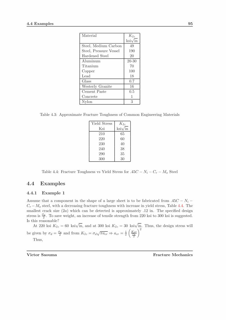
4.4 Examples 95
Material KIc
ksi√
in
Steel, Medium Carbon 49Steel, Pressure Vessel 190Hardened Steel 20
Aluminum 20-30Titanium 70Copper 100Lead 18
Glass 0.7
Westerly Granite 16
Cement Paste 0.5Concrete 1
Nylon 3
Table 4.3: Approximate Fracture Toughness of Common Engineering Materials
Yield Stress KIc
Ksi ksi√
in
210 65220 60230 40240 38290 35300 30
Table 4.4: Fracture Toughness vs Yield Stress for .45C − Ni − Cr − Mo Steel
4.4 Examples
4.4.1 Example 1
Assume that a component in the shape of a large sheet is to be fabricated from .45C − Ni −Cr −Mo steel, with a decreasing fracture toughness with increase in yield stress, Table 4.4. Thesmallest crack size (2a) which can be detected is approximately .12 in. The specified designstress is
σy
2 . To save weight, an increase of tensile strength from 220 ksi to 300 ksi is suggested.Is this reasonable?
At 220 ksi KIc = 60 ksi√
in, and at 300 ksi KIc = 30 ksi√
in. Thus, the design stress will
be given by σd =σy
2 and from KIc = σd√
πacr ⇒ acr = 1π
(KIcσy
2
)2
Thus,
Victor Saouma Fracture Mechanics
96 LEFM DESIGN EXAMPLES
Yield Stress Design Stress Fracture Toughness Critical Crack Total Crackσy σd KIc acr 2acr
220 110 60 .0947 .189300 150 30 .0127 .0255
We observe that for the first case, the total crack length is larger than the smallest one whichcan be detected (which is O.K.); Alternatively, for the second case the total critical crack size isapproximately five times smaller than the minimum flaw size required and approximately eighttimes smaller than the flaw size tolerated at the 220 ksi level.
Hence, σy should not be raised to 300 ksi.Finally, if we wanted to use the flaw size found with the 300 ksi alloy, we should have a
decrease in design stress (since KIc and acr are now set) KIc = σd√
πavis ⇒ σd = KIc√πavis
=
30ksi√
in√0.06π
= 69 ksi, with a potential factor of safety of one against cracking (we can not be sure
100% that there is no crack of that size or smaller as we can not detect it). We observe thatsince the design stress level is approximately half of that of the weaker alloy, there will be atwo fold increase in weight.
4.4.2 Example 2
A small beer barrel of diameter 15” and wall thickness of .126” made of aluminum alloy explodedwhen a pressure reduction valve malfunctioned and the barrel experienced the 610 psi fullpressure of the CO2 cylinder supplying it with gas. Afterwards, cracks approximately 4.0 inchlong by (probably) .07 inch deep were discovered on the inside of the salvaged pieces of thebarrel (it was impossible to measure their depth). Independent tests gave 40. ksi
√in for KIc of
the aluminum alloy. The question is whether the cracks were critical for the 610 psi pressure?
For a cylinder under internal pressure, the hoop stress is σ = pD2t = 610 lb
in215 in
2(.126) in =
36, 310 psi = 36.3 ksi. This can be used as the far field stress (neglecting curvature).First we use the exact solution as given in Eq. 4.24, with a = 2. in, b = .07 in, and t = .126
in. upon substitution we obtain:
M1 = 1.13 − 0.09
(.07
2.
)= 1.127
M2 = 0.89
[0.2 +
(.07
2.
)]−1
− 0.54
= 3.247
M3 = 0.5 −[0.65 +
(.07
2
)]−1
+ 14
[1. −
(.07
2
)]24= 4.994
Victor Saouma Fracture Mechanics

4.5 Additional Design Considerations 97
2c
t
2a=2t
Initial Elliptical Crack
Semicircular final crack (leak)
Figure 4.14: Growth of Semielliptical surface Flaw into Semicircular Configuration
Substituting
K = 36.3√
π.07
[1.127 + 3.247
(.07
.126
)2
+ 4.994
(.07
.126
)4] [
1 + 1.464
(.07
2
)1.65]− 1
2
[(.07
2.
)2
0 + 1
] 14{
1 +
[0.1 + 0.35
(.07
.126
)2]
(1 − 1)2}
= 44.2ksi√
in
This is about equal to the fracture toughness.Note that if we were to use the approximate equation, for long cracks we would have
obtained:
K = (1.13)(36.3)√
π(.07)
[1 + 3.46
(.07
.126
)2
+ 11.5
(.07
.126
)4]
= 60.85
> KIc
4.5 Additional Design Considerations
4.5.1 Leak Before Fail
10 As observed from the preceding example, many pressurized vessels are subject to crackgrowth if internal flaws are present. Two scenarios may happen, Fig. 4.14
Break-through: In this case critical crack configuration is reached before the crack has “day-lighted”, and there is a sudden and unstable crack growth.
Victor Saouma Fracture Mechanics

98 LEFM DESIGN EXAMPLES
Leak Before Fail: In this case, crack growth occur, and the crack “pierces” through thethickness of the vessel before unstable crack growth occurs. This in turn will result in asudden depressurization, and this will stop any further crack growth.
11 Hence, pressurized vessels should be designed to ensure a leak before fail failure scenario,as this would usually be immediately noticed and corrected (assuming that there is no leak offlammable gas!).
12 Finally, it should be noted that leak before break assessment should be made on the basis ofa complete residual strength diagram for both the part through and the through crack. Variousratios should be considered
4.5.2 Damage Tolerance Assessment
13 Fracture mechanics is not limited to determining the critical crack size, load, or stress combi-nation. It can also be applied to establish a fracture control plan, or damage tolerance analysiswith the following objectives:
1. Determine the effect of cracks on strength. This will result in a plot of crack size versusresidual strength, or Residual Strength Diagram
2. Determine crack growth with time, resulting in Crack Growth Curve.
Victor Saouma Fracture Mechanics

Chapter 5
THEORETICAL STRENGTH ofSOLIDS; (Griffith I)
1 We recall that Griffith’s involvement with fracture mechanics started as he was exploring thedisparity in strength between glass rods of different sizes, (Griffith 1921). As such, he hadpostulated that this can be explained by the presence of internal flaws (idealized as elliptical)and then used Inglis solution to explain this discrepancy.
2 In this section, we shall develop an expression for the theoretical strength of perfect crystals(theoretically the strongest form of solid). This derivation, (Kelly 1974) is fundamentallydifferent than the one of Griffith as it starts at the atomic level.
5.1 Derivation
3 We start by exploring the energy of interaction between two adjacent atoms at equilibriumseparated by a distance a0, Fig. 5.1. The total energy which must be supplied to separate atomC from C’ is
U0 = 2γ (5.1)
where γ is the surface energy1, and the factor of 2 is due to the fact that upon separation, wehave two distinct surfaces.
1 From watching raindrops and bubbles it is obvious that liquid water has surface tension. When the surfaceof a liquid is extended (soap bubble, insect walking on liquid) work is done against this tension, and energy isstored in the new surface. When insects walk on water it sinks until the surface energy just balances the decreasein its potential energy. For solids, the chemical bonds are stronger than for liquids, hence the surface energy isstronger. The reason why we do not notice it is that solids are too rigid to be distorted by it. Surface energy γis expressed in J/m2 and the surface energies of water, most solids, and diamonds are approximately .077, 1.0,and 5.14 respectively.

100 THEORETICAL STRENGTH of SOLIDS; (Griffith I)
Figure 5.1: Uniformly Stressed Layer of Atoms Separated by a0
5.1.1 Tensile Strength
5.1.1.1 Ideal Strength in Terms of Physical Parameters
We shall first derive an expression for the ideal strength in terms of physical parameters, andin the next section the strength will be expressed in terms of engineering ones.
Force being the derivative of energy, we have F = dUda , thus F = 0 at a = a0, Fig. 5.2,
and is maximum at the inflection point of the U0 − a curve. Hence, the slope of theforce displacement curve is the stiffness of the atomic spring and should be related toE. If we let x = a − a0, then the strain would be equal to ε = x
a0. Furthermore, if we
define the stress as σ = Fa20, then the σ − ε curve will be as shown in Fig. 5.3. From this
diagram, it would appear that the sine curve would be an adequate approximation to thisrelationship. Hence,
σ = σtheormax sin 2π
x
λ(5.2)
and the maximum stress σtheormax would occur at x = λ
4 . The energy required to separatetwo atoms is thus given by the area under the sine curve, and from Eq. 5.1, we wouldhave
2γ = U0 =
∫ λ2
0σtheor
max sin
(2π
x
λ
)dx (5.3)
=λ
2πσtheor
max [− cos (2πx
λ)] |
λ20 (5.4)
Victor Saouma Fracture Mechanics
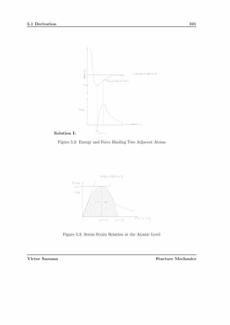
5.1 Derivation 101
Solution I:
Figure 5.2: Energy and Force Binding Two Adjacent Atoms
Figure 5.3: Stress Strain Relation at the Atomic Level
Victor Saouma Fracture Mechanics

102 THEORETICAL STRENGTH of SOLIDS; (Griffith I)
=λ
2πσtheor
max [−
−1︷ ︸︸ ︷cos (
2πλ
2λ) +
1︷ ︸︸ ︷cos(0)] (5.5)
⇒ λ =2γπ
σtheormax
(5.6)
Also for very small displacements (small x) sin x ≈ x, thus Eq. 5.2 reduces to
σ ≈ σtheormax
2πx
λ≈ E
x
a0(5.7)
elliminating x,
σtheormax ≈ E
a0
λ
2π(5.8)
Substituting for λ from Eq. 5.6, we get
σtheormax ≈
√Eγ
a0
(5.9)
Solution II: For two layers of atoms a0 apart, the strain energy per unit area due to σ (forlinear elastic systems) is
U = 12σεao
σ = Eε
}U =
σ2ao
2E(5.10)
If γ is the surface energy of the solid per unit area, then the total surface energy of twonew fracture surfaces is 2γ.
For our theoretical strength, U = 2γ ⇒ (σtheormax )2a0
2E = 2γ or σtheormax = 2
√γEa0
Note that here we have assumed that the material obeys Hooke’s Law up to failure, sincethis is seldom the case, we can simplify this approximation to:
σtheormax =
√Eγ
a0
(5.11)
which is the same as Equation 5.9
Example: As an example, let us consider steel which has the following properties: γ = 1 Jm2 ;
E = 2 × 10¹¹ Nm2 ; and a0 ≈ 2 × 10⁻¹⁰ m. Thus from Eq. 5.9 we would have:
σtheormax ≈
√(2 × 10¹¹)(1)
2 × 10⁻¹⁰(5.12)
≈ 3.16 × 10¹⁰ N
m2(5.13)
≈ E
6(5.14)
Thus this would be the ideal theoretical strength of steel.
Victor Saouma Fracture Mechanics

5.1 Derivation 103
5.1.1.2 Ideal Strength in Terms of Engineering Parameter
We note that the force to separate two atoms drops to zero when the distance between themis a0 + a where a0 corresponds to the origin and a to λ
2 . Thus, if we take a = λ2 or λ = 2a,
combined with Eq. 5.8 would yield
σtheormax ≈ E
a0
a
π(5.15)
4 Alternatively combining Eq. 5.6 with λ = 2a gives
a ≈ γπ
σtheormax
(5.16)
5 Combining those two equations
γ ≈ E
a0
(a
π
)2
(5.17)
6 However, since as a first order approximation a ≈ a0 then the surface energy will be
γ ≈ Ea0
10(5.18)
7 This equation, combined with Eq. 5.9 will finally give
σtheormax ≈ E√
10(5.19)
which is an approximate expression for the theoretical maximum strength in terms of E.
5.1.2 Shear Strength
8 Similar derivation can be done for shear. What happen if we slide the top row over thebottom one. Again, we can assume that the shear stress is
τ = τ theormax sin 2π
x
λ(5.20)
and from basic elasticityτ = Gγxy (5.21)
and, Fig. 5.4 γxy = x/h.
9 Because we do have very small displacement, we can elliminate x from
τ theormax sin 2π
x
λ� 2πx
λ= γG =
x
hG
⇒ τ theormax =
Gλ
2πh(5.22-a)
Victor Saouma Fracture Mechanics

104 THEORETICAL STRENGTH of SOLIDS; (Griffith I)
x
h
Figure 5.4: Influence of Atomic Misfit on Ideal Shear Strength
10 If we do also assume that λ = h, and G = E/2(1 + ν), then
τ theormax � E
12(1 + ν)� E
18(5.23)
5.2 Griffith Theory
11 Around 1920, Griffith was exploring the theoretical strength of solids by performing a se-ries of experiments on glass rods of various diameters. He observed that the tensile strength(σt) of glass decreased with an increase in diameter, and that for a diameter φ ≈ 1
10,000 in.,σt = 500, 000 psi; furthermore, by extrapolation to “zero” diameter he obtained a theoreti-cal maximum strength of approximately 1,600,000 psi, and on the other hand for very largediameters the asymptotic values was around 25,000 psi.
12 Griffith had thus demonstrated that the theoretical strength could be experimentally ap-proached, he now needed to show why the great majority of solids fell so far below it.
5.2.1 Derivation
13 In his quest for an explanation, he came across Inglis’s paper, and his “strike of genius” wasto assume that strength is reduced due to the presence of internal flaws. Griffith postulatedthat the theoretical strength can only be reached at the point of highest stress concentration,and accordingly the far-field applied stress will be much smaller.
14 Hence, assuming an elliptical imperfection, and from equation 3.29
σtheormax = σact
cr
(1 + 2
√a
ρ
)(5.24)
σ is the stress at the tip of the ellipse which is caused by a (lower) far field stress σactcr .
Victor Saouma Fracture Mechanics

5.2 Griffith Theory 105
15 Asssuming ρ ≈ a0 and since 2√
aa0
� 1, for an ideal plate under tension with only one single
elliptical flaw the strength may be obtained from
σtheormax︸ ︷︷ ︸
micro
= 2σactcr
√a
a0︸ ︷︷ ︸macro
(5.25)
hence, equating with Eq. 5.9, we obtain
σtheormax = 2σact
cr
√a
ao︸ ︷︷ ︸Macro
=
√Eγ
a0︸ ︷︷ ︸Micro
(5.26)
16 From this very important equation, we observe that
1. The left hand side is based on a linear elastic solution of a macroscopic problem solvedby Inglis.
2. The right hand side is based on the theoretical strength derived from the sinusoidal stress-strain assumption of the interatomic forces, and finds its roots in micro-physics.
17 Finally, this equation would give (at fracture)
σactcr =
√Eγ
4a(5.27)
18 As an example, let us consider a flaw with a size of 2a = 5, 000a0
σactcr =
√Eγ4a
γ = Ea010
}σact
cr =√
E2
40ao
aaa0
= 2, 500
}σact
cr =√
E2
100,000 = E100
√10
(5.28)
19 Thus if we set a flaw size of 2a = 5, 000a0 in γ ≈ Ea010 this is enough to lower the theoretical
fracture strength from E√10
to a critical value of magnitude E100
√10
, or a factor of 100.
20 Also
σtheormax = 2σact
cr
√aao
a = 10−6m = 1μmao = 1A = ρ = 10−10m
⎫⎪⎬⎪⎭σtheor
max = 2σactcr
√10−6
10−10= 200σact
cr (5.29)
21 Therefore at failure
σactcr = σtheor
max
200
σtheormax = E
10
}σact
cr ≈ E
2, 000(5.30)
which can be attained. For instance for steel E2,000 = 30,000
2,000 = 15 ksi
Victor Saouma Fracture Mechanics

106 THEORETICAL STRENGTH of SOLIDS; (Griffith I)
Victor Saouma Fracture Mechanics

Chapter 6
ENERGY TRANSFER in CRACKGROWTH; (Griffith II)
1 In the preceding chapters, we have focused on the singular stress field around a crack tip. Onthis basis, a criteria for crack propagation, based on the strength of the singularity was firstdeveloped and then used in practical problems.
2 An alternative to this approach, is one based on energy transfer (or release), which occursduring crack propagation. This dual approach will be developed in this chapter.
3 Griffith’s main achievement, in providing a basis for the fracture strengths of bodies containingcracks, was his realization that it was possible to derive a thermodynamic criterion for fractureby considering the total change in energy of a cracked body as the crack length increases,(Griffith 1921).
4 Hence, Griffith showed that material fail not because of a maximum stress, but rather becausea certain energy criteria was met.
5 Thus, the Griffith model for elastic solids, and the subsequent one by Irwin and Orowan forelastic-plastic solids, show that crack propagation is caused by a transfer of energy transferfrom external work and/or strain energy to surface energy.
6 It should be noted that this is a global energy approach, which was developed prior to theone of Westergaard which focused on the stress field surrounding a crack tip. It will be shownlater that for linear elastic solids the two approaches are identical.

108 ENERGY TRANSFER in CRACK GROWTH; (Griffith II)
6.1 Thermodynamics of Crack Growth
6.1.1 General Derivation
7 If we consider a crack in a deformable continuum subjected to arbitrary loading, then thefirst law of thermodynamics gives: The change in energy is proportional to the amount of workperformed. Since only the change of energy is involved, any datum can be used as a basis formeasure of energy. Hence energy is neither created nor consumed.
8 The first law of thermodynamics states The time-rate of change of the total energy (i.e., sumof the kinetic energy and the internal energy) is equal to the sum of the rate of work done bythe external forces and the change of heat content per unit time:
d
dt(K + U + Γ) = W + Q (6.1)
where K is the kinetic energy, U the total internal strain energy (elastic plus plastic), Γ thesurface energy, W the external work, and Q the heat input to the system.
9 Since all changes with respect to time are caused by changes in crack size, we can write
∂
∂t=
∂A
∂t
∂
∂A(6.2)
and for an adiabatic system (no heat exchange) and if loads are applied in a quasi staticmanner (no kinetic energy), then Q and K are equal to zero, and for a unit thickness we canreplace A by a, then we can rewrite the first law as
∂W
∂a︸ ︷︷ ︸External
=
(∂U e
∂a+
∂Up
∂a
)+
∂Γ
∂a︸ ︷︷ ︸Internal
(6.3)
10 This equation represents the energy balance during crack growth. It indicates that the workrate supplied to the continuum by the applied external loads is equal to the rate of strain energy(elastic and plastic) dissipated during crack propagation.
11 Thus
Π ≡ U e − W∂Π∂a = ∂Ue
∂a + ∂W∂a
= ∂Ue
∂a + −∂Ue
∂a − ∂Up
∂a − ∂Γ∂a
(6.4)
or
− ∂Π
∂a=
∂Up
∂a+
∂Γ
∂a(6.5)
Victor Saouma Fracture Mechanics

6.1 Thermodynamics of Crack Growth 109
that is the rate of potential energy decrease during crack growth is equal to the rate of energydissipated in plastic deformation and crack growth.
12 It is very important to observe that the energy scales with a2, whereas surface energy scaleswith a. It will be shown later that this can have serious implication on the stability of cracks,and on size effects.
6.1.2 Brittle Material, Griffith’s Model
13 For a perfectly brittle material, we can rewrite Eq. 6.3 as
Gdef= −∂Π
∂a=
∂W
∂a− ∂U e
∂a=
∂Γ
∂a= 2γ (6.6)
the factor 2 appears because we have two material surfaces upon fracture. The left hand siderepresents the energy available for crack growth and is given the symbol G in honor of Griffith.Because G is derived from a potential function, it is often referred to as the crack driving force.The right hand side represents the resistance of the material that must be overcome for crackgrowth, and is a material constant (related to the toughness).
14 This equation represents the fracture criterion for crack growth, two limiting cases can beconsidered. They will be examined in conjunction with Fig. 6.1 in which we have a crack oflength 2a located in an infinite plate subjected to load P . Griffith assumed that it was possible
Figure 6.1: Energy Transfer in a Cracked Plate
Victor Saouma Fracture Mechanics
110 ENERGY TRANSFER in CRACK GROWTH; (Griffith II)
to produce a macroscopical load displacement (P − u) curve for two different crack lengths aand a + da.
Two different boundary conditions will be considered, and in each one the change in potentialenergy as the crack extends from a to a + da will be determined:
Fixed Grip: (u2 = u1) loading, an increase in crack length from a to a + da results in adecrease in stored elastic strain energy, ΔU ,
ΔU =1
2P2u1 −
1
2P1u1 (6.7)
=1
2(P2 − P1) u1 (6.8)
< 0 (6.9)
Furthermore, under fixed grip there is no external work (u2 = u1), so the decrease inpotential energy is the same as the decrease in stored internal strain energy, hence
Π2 − Π1 = ΔW − ΔU (6.10)
= −1
2(P2 − P1)u1 =
1
2(P1 − P2)u1 (6.11)
Fixed Load: P2 = P1 the situation is slightly more complicated. Here there is both externalwork
ΔW = P1(u2 − u1) (6.12)
and a release of internal strain energy. Thus the net effect is a change in potential energygiven by:
Π2 − Π1 = ΔW − ΔU (6.13)
= P1 (u2 − u1) −1
2P1 (u2 − u1) (6.14)
=1
2P1 (u2 − u1) (6.15)
= Γ (6.16)
15 Thus under fixed grip conditions there is a decrease in strain energy of magnitude 12u1(P1−P2)
as the crack extends from a to (a + Δa), whereas under constant load, there is a net decreasein potential energy of magnitude 1
2P1(u2 − u1).
16 At the limit as Δa → da, we define:
dP = P1 − P2 (6.17)
du = u2 − u1 (6.18)
Victor Saouma Fracture Mechanics

6.1 Thermodynamics of Crack Growth 111
then as da → 0, the decrease in strain energy (and potential energy in this case) for the fixedgrip would be
dΠ =1
2udP (6.19)
and for the constant load case
dΠ =1
2Pdu (6.20)
17 Furthermore, defining the compliance as
u = CP (6.21)
du = CdP (6.22)
18 Then the decrease in potential energy for both cases will be given by
dΠ =1
2CP dP (6.23)
19 In summary, as the crack extends there is a release of excess energy. Under fixedgrip conditions, this energy is released from the strain energy. Under fixed load condition,external work is produced, half of it is consumed into strain energy, and the other half released.In either case, the energy released is consumed to form surface energy.
20 Thus a criteria for crack propagation would be
dΠ ≥ 2γda (6.24)
The difference between the two sides of the inequality will appear as kinetic energy at a realcrack propagation.
Energy Release Rate per unit crack extension = Surface energy
dΠ
da= 2γ (6.25)
21 Using Inglis solution, Griffith has shown that for plane stress infinite plates with a centralcrack of length 2a1
− dΠ
da=
πaσ2cr
E(6.26)
note that the negative sign is due to the decrease in energy during crack growth. Combiningwith Eq. 6.25, and for incipient crack growth, this reduces to
σ2crπada
E′ = 2γda (6.27)
1This equation will be rederived in Sect. 6.4 using Westergaard’s solution.
Victor Saouma Fracture Mechanics

112 ENERGY TRANSFER in CRACK GROWTH; (Griffith II)
i
Ai+1
i+1B
A
u
P
a5a4
a3a2
a1
P
u
P
P
u u
i
iO
A1
A2
A3A4
A5
i+1
i+1
iB
x
x
xx
x
Figure 6.2: Determination of Gc From Load Displacement Curves
or
σcr =
√2E′γπa
(6.28)
This equation derived on the basis of global fracture should be compared with Eq. 5.11 derivedfrom local stress analysis.
6.2 Energy Release Rate; Global
6.2.1 From Load-Displacement
22 With reference to Fig. 6.2 The energy released, for unit crack surface, from increment i toincrement i + 1 is given by
G =∑
i=1,n
OAiAi+1
ai+1 − ai(6.29)
where
OAiAi+1 = (OAiBi) + (AiBiBi+1Ai+1) − (OAi+1Bi+1) (6.30-a)
=1
2Piui +
1
2(Pi + Pi+1)(ui+1 − ui) −
1
2Pi+1ui+1 (6.30-b)
=1
2(Piui+1 − Pi+1ui) (6.30-c)
Thus, the critical energy release rate will be given by
G =∑
i=1,n
1
2B
Piui+1 − Pi+1ui
ai+1 − ai(6.31)
where B is the thickness.
Victor Saouma Fracture Mechanics

6.2 Energy Release Rate; Global 113
6.2.2 From Compliance
23 Under constant load we found the energy release needed to extend a crack by da was 12Pdu.
If G is the energy release rate, B is the thickness, and u = CP , (where u, C and P are thepoint load displacement, compliance and the load respectively), then
GBda =1
2Pd(CP ) =
1
2P 2dC (6.32)
at the limit as da → 0, then we would have:
G =1
2
P 2
B
(dC
da
)(6.33)
24 Thus we can use an experimental technique to obtain G and from G =K2
I
E′ (to be derivedlater) to get KI , Fig. 6.3
Figure 6.3: Experimental Determination of KI from Compliance Curve
25 With regard to accuracy since we are after K which does not depend on E, a low modulusplate material (i.e. high strength aluminum) can be used to increase observed displacement.
26 As an example, let us consider the double cantilever beam problem, Fig. 6.4. From strengthof materials:
C =24
EB
∫ a
0
x2
h3dx︸ ︷︷ ︸
flexural
+6(1 + ν)
EB
∫ a
0
1
hdx︸ ︷︷ ︸
shear
(6.34)
Taking ν = 13 we obtain
C =8
EB
∫ a
0
(3x2
h3+
1
h
)dx (6.35)
Victor Saouma Fracture Mechanics

114 ENERGY TRANSFER in CRACK GROWTH; (Griffith II)
Figure 6.4: KI for DCB using the Compliance Method
dC
da=
8
EB
(3a2
h3+
1
h
)(6.36)
Substituting in Eq. 6.33
G =1
2
P 2
B
(dc
da
)(6.37)
=1
2
P 28
EB2
(3a2
h3+
1
h
)(6.38)
=4P 2
EB2h3
(3a2 + h2
)(6.39)
Thus the stress intensity factor will be
K =√
GE =2P
B
(3a2
h3+
1
h
) 12
(6.40)
27 Had we kept G in terms of ν
G =4P 2
EB2h3
[3a2 +
3
4h2(1 + ν)
](6.41)
28 We observe that in this case K increases with a, hence we would have an unstable crackgrowth. Had we had a beam in which B increases with a, Fig. 6.5, such that
3a2
h3+
1
h= m = Cst (6.42)
then
K =2P
Bm
12 (6.43)
Such a specimen, in which K remains constant as a increases was proposed by Mostovoy(Mostovoy 1967) for fatigue testing.
Victor Saouma Fracture Mechanics
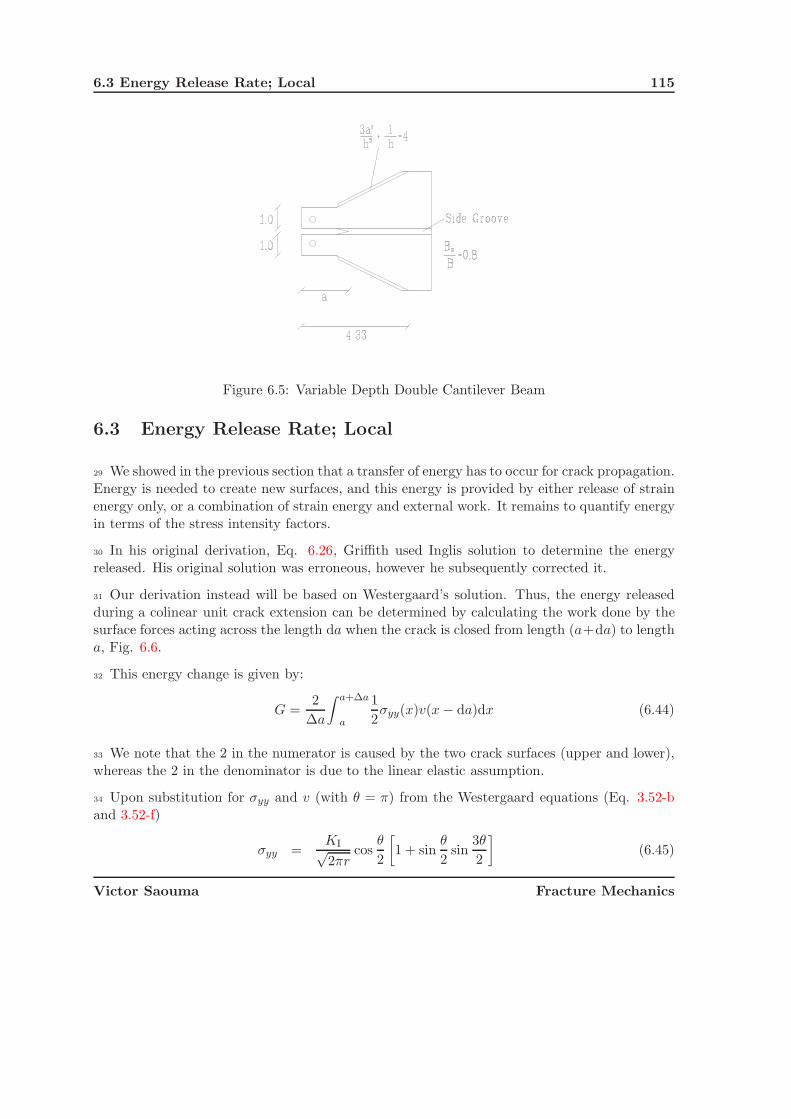
6.3 Energy Release Rate; Local 115
Figure 6.5: Variable Depth Double Cantilever Beam
6.3 Energy Release Rate; Local
29 We showed in the previous section that a transfer of energy has to occur for crack propagation.Energy is needed to create new surfaces, and this energy is provided by either release of strainenergy only, or a combination of strain energy and external work. It remains to quantify energyin terms of the stress intensity factors.
30 In his original derivation, Eq. 6.26, Griffith used Inglis solution to determine the energyreleased. His original solution was erroneous, however he subsequently corrected it.
31 Our derivation instead will be based on Westergaard’s solution. Thus, the energy releasedduring a colinear unit crack extension can be determined by calculating the work done by thesurface forces acting across the length da when the crack is closed from length (a+da) to lengtha, Fig. 6.6.
32 This energy change is given by:
G =2
Δa
∫ a+Δa
a
1
2σyy(x)v(x − da)dx (6.44)
33 We note that the 2 in the numerator is caused by the two crack surfaces (upper and lower),whereas the 2 in the denominator is due to the linear elastic assumption.
34 Upon substitution for σyy and v (with θ = π) from the Westergaard equations (Eq. 3.52-band 3.52-f)
σyy =KI√2πr
cosθ
2
[1 + sin
θ
2sin
3θ
2
](6.45)
Victor Saouma Fracture Mechanics
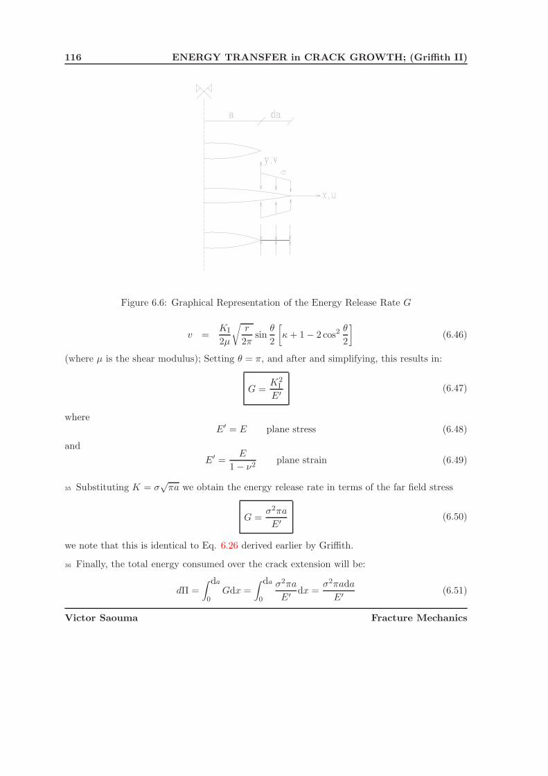
116 ENERGY TRANSFER in CRACK GROWTH; (Griffith II)
Figure 6.6: Graphical Representation of the Energy Release Rate G
v =KI
2μ
√r
2πsin
θ
2
[κ + 1 − 2 cos2 θ
2
](6.46)
(where μ is the shear modulus); Setting θ = π, and after and simplifying, this results in:
G =K2
I
E′ (6.47)
whereE′ = E plane stress (6.48)
and
E′ =E
1 − ν2plane strain (6.49)
35 Substituting K = σ√
πa we obtain the energy release rate in terms of the far field stress
G =σ2πa
E′ (6.50)
we note that this is identical to Eq. 6.26 derived earlier by Griffith.
36 Finally, the total energy consumed over the crack extension will be:
dΠ =
∫ da
0Gdx =
∫ da
0
σ2πa
E′ dx =σ2πada
E′ (6.51)
Victor Saouma Fracture Mechanics

6.4 Crack Stability 117
37 Sih, Paris and Irwin, (Sih et al. 1965), developed a counterpar to Equation 6.47 for anisotropicmaterials as
G =
√(a11a22
2
)(√a11
a22+
2a12 + a66
2a22
)K2 (6.52)
6.4 Crack Stability
38 Crack stability depends on both the geometry, and on the material resistance.
6.4.1 Effect of Geometry; Π Curve
39 From Eq. 6.6, crack growth is considered unstable when the energy at equilibrium is amaximum, and stable when it is a minimum. Hence, a sufficient condition for crack stabilityis, (Gdoutos 1993)
∂2(Π + Γ)
∂A2
⎧⎪⎨⎪⎩
< 0 unstable fracture> 0 stable fracture= 0 neutral equilibrium
(6.53)
and the potential energy is Π = U − W .
40 If we consider a line crack in an infinite plate subjected to uniform stress, Fig. 6.7, then thepotential energy of the system is Π = U e where Eq. 6.6 yields
KI = σ√
πa (6.54-a)
G =K2
I
E′ (6.54-b)
=σ2πa
E′ (6.54-c)
Π = U e =
∫Gda (6.54-d)
= −1
2
σ2πa2
E′ (6.54-e)
and Γ = 4a (crack length is 2a). Note that U e is negative because there is a decrease in strainenergy during crack propagation. If we plot Γ, Π and Γ + Π, Fig. 6.7, then we observe thatthe total potential energy of the system (Π + Γ) is maximum at the critical crack length whichcorresponds to unstable equilibrium.
41 If we now consider the cleavage of mica, a wedge of thickness h is inserted under a flakeof mica which is detached from a mica block along a length a. The energy of the system isdetermined by considering the mica flake as a cantilever beam with depth d. From beam theory
U e =Ed3h2
8a3(6.55)
Victor Saouma Fracture Mechanics
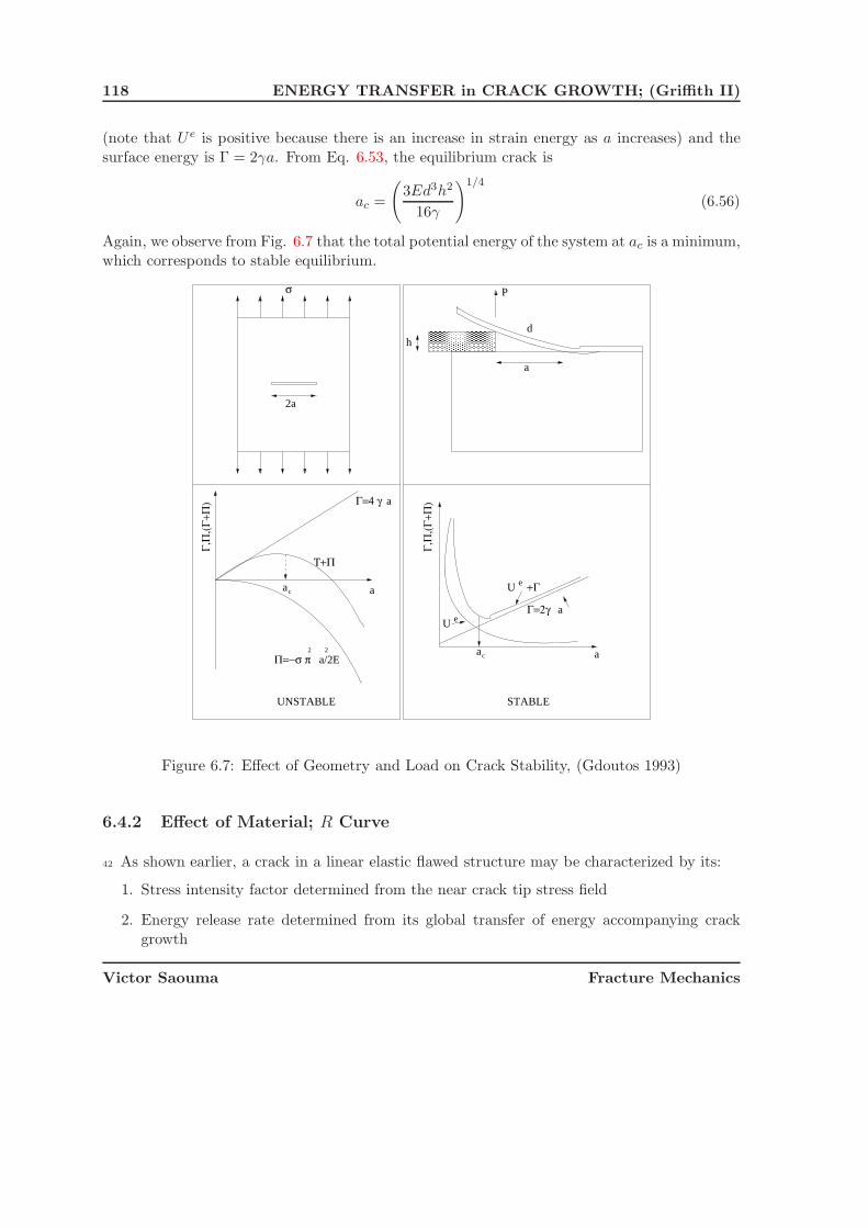
118 ENERGY TRANSFER in CRACK GROWTH; (Griffith II)
(note that U e is positive because there is an increase in strain energy as a increases) and thesurface energy is Γ = 2γa. From Eq. 6.53, the equilibrium crack is
ac =
(3Ed3h2
16γ
)1/4
(6.56)
Again, we observe from Fig. 6.7 that the total potential energy of the system at ac is a minimum,which corresponds to stable equilibrium.
Γ=4 γ a
ac
ac
U e
U e
2a
h
P
a
d
σ
Τ+Π
Γ,Π
,(Γ+Π
)
Γ,Π
,(Γ+Π
)
a
a
a
+Γ
a/2E
UNSTABLE STABLE
Γ=2γ
Π=−σ π2 2
Figure 6.7: Effect of Geometry and Load on Crack Stability, (Gdoutos 1993)
6.4.2 Effect of Material; R Curve
42 As shown earlier, a crack in a linear elastic flawed structure may be characterized by its:
1. Stress intensity factor determined from the near crack tip stress field
2. Energy release rate determined from its global transfer of energy accompanying crackgrowth
Victor Saouma Fracture Mechanics
6.4 Crack Stability 119
43 Thus for a crack to extend, two criteria are possible:
1. Compare the stress intensity factor K with a material property called the critical stressintensity factor KIc, or fracture toughness.
2. Compare the energy release rate G with a material property called the critical energyrelease rate GIc.
6.4.2.1 Theoretical Basis
44 Revisiting Eq. 6.3∂W
∂a=
(∂U e
∂a+
∂Up
∂a
)+
∂Γ
∂a(6.57)
we can rewrite it as∂W
∂a− ∂U e
∂a︸ ︷︷ ︸G
=∂Up
∂a+
∂Γ
∂a︸ ︷︷ ︸R
(6.58)
where R represents the rate of energy dissipation during stable crack growth. The first partcorresponds to plastic deformation, and the second to energy consumed during crack propaga-tion.
6.4.2.2 R vs KIc
45 Back to Eq. 6.51, crack instability will occur when for an infinitesimal crack extension da,the rate of energy released is just equal to surface energy absorbed.
σ2crπada
E′︸ ︷︷ ︸dΠ
= 2γda (6.59)
or
σcr =
√2E′γπa
(6.60)
Which is Eq. 6.28 as originally derived by Griffith (Griffith 1921).
46 This equation can be rewritten as
σ2crπa
E′︸ ︷︷ ︸Gcr
≡ R︸︷︷︸2γ
(6.61)
and asσcr
√πa =
√2E′γ = KIc (6.62)
Victor Saouma Fracture Mechanics

120 ENERGY TRANSFER in CRACK GROWTH; (Griffith II)
thus
Gcr = R =K2
Ic
E′ (6.63)
47 In general, the critical energy release rate is defined as R (for Resistance) and is only equalto a constant (Gcr) under plane strain conditions.
48 Critical energy release rate for plane stress is found not to be constant, thus KIc is notconstant, and we will instead use K1c and G1c. Alternatively, KIc, and GIc correspond to planestrain in mode I which is constant. Hence, the shape of the R-curve depends on the platethickness, where plane strain is approached for thick plates, and is constant; and for thin plateswe do not have constant R due to plane stress conditions.
49 Using this energetic approach, we observe that contrarily to the Westergaard/Irwin criteriawhere we zoomed on the crack tip, a global energy change can predict a local event (crackgrowth).
50 The duality between energy and stress approach G > Gcr = R, or K > KIc, should also benoted.
51 Whereas the Westergaard/Irwin criteria can be generalized to mixed mode loading (in chap-ter 7), the energy release rate for mixed mode loading (where crack extension is not necessarilycollinear with the crack axis) was not derived until 1974 by Hussain et al. (Hussain, Pu andUnderwood 1974). However, should we assume a collinear crack extension under mixed modeloading, then
G = GI + GII + GIII =1 − ν2
E(K2
I + K2II +
K2III
1 − ν) (6.64)
52 From above, we have the energy release rate given by
G =σ2πa
E′ (6.65)
and the critical energy release rate is
R = Gcr =dΠ
da= 2γ =
K2Ic
E′ (6.66)
53 Criteria for crack growth can best be understood through a graphical representation of thosecurves under plane strain and plane stress conditions.
6.4.2.3 Plane Strain
54 For plane strain conditions, the R curve is constant and is equal to GIc. Using Fig. 6.8 FromEq. 6.65, G = σ2πa
E′ , G is always a linear function of a, thus must be a straight line.
Victor Saouma Fracture Mechanics

6.4 Crack Stability 121
2
σ1
σ2
σ2
Δ
R=G Ic
R=G
R=G
a1
aa
a
1σ
Δ
σ
2
2
Ic
σ1
a1
Ic
a
G,R
a
A C
B
νπ a
E
22
νπ a
E
22σ
2G=(1- )
G=(1- )
G,R Constant Grip
Constant Load
σ
σ
K NG,R
H
FL
Figure 6.8: R Curve for Plane Strain
Victor Saouma Fracture Mechanics

122 ENERGY TRANSFER in CRACK GROWTH; (Griffith II)
55 For plane strain problems, if the crack size is a1, the energy release rate at a stress σ2 isrepresented by point B. If we increase the stress from σ2 to σ1, we raise the G value from B toA. At A, the crack will extend. Had we had a longer crack a2, it would have extended at σ2.
56 Alternatively, we can plot to the right Δa, and to the left the original crack length ai. At astress σ2, the G line is given by LF (really only point F). So by loading the crack from 0 to σ2,G increases from O to F, further increase of the stress to σ1 raises G from F to H, and thenfracture occurs, and the crack goes from H to K. On the other hand, had we had a crack oflength a2 loaded from 0 to σ2, its G value increases from O to H (note that LF and MH areparallel). At H crack extension occurs along HN.
57 Finally, it should be noted that depending on the boundary conditions, G may increaselinearly (constant load) or as a polynomial (fixed grips).
6.4.2.4 Plane Stress
58 Under plane strain R was independent of the crack length. However, under plane stress Ris found to be an increasing function of a, Fig. 6.9
G,R
F
RD
H
C
BA
a Δ ai
σc σ σ
σ1
23
Figure 6.9: R Curve for Plane Stress
59 If we examine an initial crack of length ai:
1. under σ1 at point A, G < R, thus there is no crack extension.
2. If we increase σ1 to σ2, point B, then G = R and the crack propagates by a small incrementΔa and will immediately stop as G becomes smaller than R.
3. if we now increase σ1 to σ3, (point C) then G > R and the crack extends to a + Δa. G
Victor Saouma Fracture Mechanics

6.4 Crack Stability 123
increases to H, however, this increase is at a lower rate than the increase in R
dG
da<
dR
da(6.67)
thus the crack will stabilize and we would have had a stable crack growth.
4. Finally, if we increase σ1 to σc, then not only is G equal to R, but it grows faster than Rthus we would have an unstable crack growth.
60 From this simple illustrative example we conclude that
Stable Crack Growth: G > R dGda
< dRda
Unstable Crack Growth: G > R dGda
> dRda
(6.68)
we also observe that for unstable crack growth, excess energy is transformed into kinetic energy.
61 Finally, we note that these equations are equivalent to Eq. 6.53 where the potential energyhas been expressed in terms of G, and the surface energy expressed in terms of R.
62 Some materials exhibit a flat R curve, while other have an ascending one. The shape of theR curve is a material property. For ideally brittle material, R is flat since the surface energyγ is constant. Nonlinear material would have a small plastic zone at the tip of the crack. Thedriving force in this case must increase. If the plastic zone is small compared to the crack (aswould be eventually the case for sufficiently long crack in a large body), then R would approacha constant value.
63 The thickness of the cracked body can also play an important role. For thin sheets, the loadis predominantly plane stress, Fig. 6.10.
64 Alternatively, for a thick plate it would be predominantly plane strain. Hence a plane stressconfiguration would have a steeper R curve.
Victor Saouma Fracture Mechanics

124 ENERGY TRANSFER in CRACK GROWTH; (Griffith II)
Figure 6.10: Plastic Zone Ahead of a Crack Tip Through the Thickness
Victor Saouma Fracture Mechanics

Chapter 7
MIXED MODE CRACKPROPAGATION
1 Practical engineering cracked structures are subjected to mixed mode loading, thus in generalKI and KII are both nonzero, yet we usually measure only mode I fracture toughness KIc (KIIc
concept is seldom used). Thus, so far the only fracture propagation criterion we have is formode I only (KI vs KIc, and GI vs R).
2 Whereas under pure mode I in homogeneous isotropic material, crack propagation is collinear,in all other cases the propagation will be curvilinear and at an angle θ0 with respect to thecrack axis. Thus, for the general mixed mode case, we seek to formulate a criterion that willdetermine:
1. The angle of incipient propagation, θ0, with respect to the crack axis.
2. If the stress intensity factors are in such a critical combination as to render the cracklocally unstable and force it to propagate.
3 Once again, for pure mode I problems, fracture initiation occurs if:
KI ≥ KIc (7.1)
4 The determination of a fracture initiation criterion for an existing crack in mode I and IIwould require a relationship between KI,KII, and KIc of the form
F (KI,KII,KIc) = 0 (7.2)
and would be analogous to the one between the two principal stresses and a yield stress, Fig.7.1
Fyld(σ1, σ2, σy) = 0 (7.3)

126 MIXED MODE CRACK PROPAGATION
Figure 7.1: Mixed Mode Crack Propagation and Biaxial Failure Modes
Such an equation may be the familiar von Mises criterion.
5 In the absence of a widely accepted criterion for mixed mode crack growth, three of the mostwidely used criterion are discussed below.
7.1 Analytical Models for Isotropic Solids
6 First four models for the mixed mode crack propagation will be presented, three for isotropicmaterials, and one for anisotropic ones. Subsequently the actual algorithmic implementationof those models will be presented.
7.1.1 Maximum Circumferential Tensile Stress.
7 Erdogan, F. and Sih, G.C. (1963) presented the first mixed-mode fracture initiation theory,the maximum circumferential tensile stress theory. It is based on the knowledge of the stressstate near the tip of a crack, written in polar coordinates.
8 The maximum circumferential stress theory states that the crack extension starts:
1. At its tip in a radial direction
2. In the plane perpendicular to the direction of greatest tension, i.e at an angle θ0 such thatτrθ = 0
3. When σθmax reaches a critical material constant
Victor Saouma Fracture Mechanics

7.1 Analytical Models for Isotropic Solids 127
9 It can be easily shown that σθ reaches its maximum value when τrθ = 0. Replacing τrθ formode I and II by their expressions given in Eq. 3.55-c and 3.56-c
τrθ =KI√2πr
sinθ
2cos2 θ
2+
KII√2πr
(1
4cos
θ
2+
3
4cos
3θ
2
)(7.4)
⇒ cosθ0
2[KI sin θ0 + KII (3 cos θ0 − 1)] = 0 (7.5)
this equation has two solutions:
θ0 = ±π trivial (7.6)
KI sin θ0 + KII (3 cos θ0 − 1) = 0 (7.7)
Solution of the second equation yields the angle of crack extension θ0
tanθ0
2=
1
4
KI
KII± 1
4
√(KI
KII
)2
+ 8 (7.8)
10 For the crack to extend, the maximum circumferential tensile stress, σθ (from Eq. 3.55-band 3.56-b)
σθ =KI√2πr
cosθ0
2
(1 − sin2 θ0
2
)+
KII√2πr
(−3
4sin
θ0
2− 3
4sin
3θ0
2
)(7.9)
must reach a critical value which is obtained by rearranging the previous equation
σθmax
√2πr = KIc = cos
θ0
2
[KI cos2 θ0
2− 3
2KII sin θ0
](7.10)
which can be normalized as
KI
KIccos3
θ0
2− 3
2
KII
KIccos
θ0
2sin θ0 = 1 (7.11)
11 This equation can be used to define an equivalent stress intensity factor Keq for mixed modeproblems
Keq = KI cos3 θ0
2− 3
2KII cos
θ0
2sin θ0 (7.12)
7.1.2 Maximum Energy Release Rate
12 In their original model, Erdogan, F. and Sih, G.C. (1963) noted that:
Victor Saouma Fracture Mechanics

128 MIXED MODE CRACK PROPAGATION
“If we accept Griffith (energy) theory as the valid criteria which explains crackgrowth, then the crack will grow in the direction along which the elastic energyrelease per unit crack extension will be maximum and the crack will start to growwhen this energy reaches a critical value (or G = G(δ, θ)). Evaluation of G(δ, θ)poses insurmountable mathematical difficulties.”
13 Finding G(δ, θ) will establish for the general mixed mode case the duality which is the basisof fracture mechanics: the equivalence in viewing fracture initiation from either a global energybalance or a local stress intensity point of view.
14 This (insurmountable) problem was solved in 1974, by Hussain et al. (1974). Fundamentally,Hussain et al. (1974) have solved for the stress intensity factor of a major crack with an infin-itesimal “kink” at an angle θ, KI(θ) and KII(θ) in terms of the stress intensity factors of theoriginal crack KI and KII , Fig. 7.2:
Figure 7.2: Crack with an Infinitesimal “kink” at Angle θ
{KI(θ)KII(θ)
}=
(4
3 + cos2 θ
)(1 − θ
π
1 + θπ
) θ2π{
KI cos θ + 32KII sin θ
KII cos θ − 12KI sin θ
}(7.13)
15 Those expressions of KI(θ) and KII(θ) were then substituted into Irwin’s generalized ex-pression for the energy release rate (assuming collinear crack growth), Eq. 6.64
G(θ) =1
E′(K2
I (θ) + K2II(θ)
)(7.14)
yielding
G(θ) =4
E′
(1
3 + cos2 θ
)2(
1 − θπ
1 + θπ
) θπ
[(1 + 3 cos2 θ)K2I + 8 sin θ cos θKIKII + (9 − 5 cos2 θ)K2
II ] (7.15)
Victor Saouma Fracture Mechanics

7.1 Analytical Models for Isotropic Solids 129
16 The angle of crack propagation θ0 is found by maximizing G(θ);
∂G(θ)
∂θ= 0 (7.16)
∂2G(θ)
∂θ2< 0 (7.17)
For pure mode II (KI = 0), it is found that θ0 = 75.2o
17 If crack extension occurs when G reaches a critical value which is the same scalar quantity
for all cases, then this critical value can be determined by setting KII = 0 and Gcr =K2
Icr
E ;thus, substituting in Eq. 7.15
4
(1
3 + cos2 θ0
)2(
1 − θ0π
1 + θ0π
) θ0π
[(1 + 3 cos2 θ0
)( KI
KIc
)2
+ 8 sin θ0 cos θ0
(KIKII
K2Ic
)+(9 − 5 cos2 θ0
)(KII
KIc
)2]
= 1
7.1.3 Minimum Strain Energy Density Criteria.
18 The minimum strain energy density theory, formulated by Sih (1974), postulates that afracture initiates from the crack tip in a direction θ0, along which the strain energy density at acritical distance is a minimum (i.e. crack propagates along path of minimum resistance), whenthis minimum reaches a critical value.
19 The strain energy density dW per unit volume dV is
dW
dV=
1
2E(σ2
xx + σ2yy + σ2
zz) −ν
E(σxxσyy + σyyσzz + σzzσxx) +
1
2μ(τ2
xy + τ2yz + τ2
zx) (7.18)
where μ is the shear modulus (often referred to as G).
20 In two dimensional problems, this equation reduces to:
dW
dV=
1
4μ
[κ + 1
4(σxx + σyy)
2 − 2(σxxσyy − τ2xy)
](7.19)
where κ = 3 − 4ν plane strain, and κ = 3−ν1+ν for plane stress.
21 Using Westergaard’s solution for a cracked infinite plate and substituting the stress into Eq.
7.29, dWdV
, we obtain
∂W
∂V=
1
r0π
(a11K
2I + 2a12KIKII + a22K
2II
)=
S(θ)
r0(7.20)
Victor Saouma Fracture Mechanics
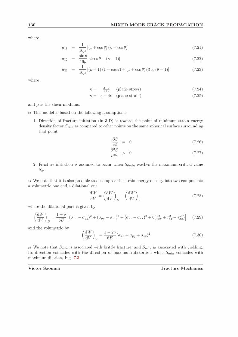
130 MIXED MODE CRACK PROPAGATION
where
a11 =1
16μ[(1 + cos θ) (κ − cos θ)] (7.21)
a12 =sin θ
16μ[2 cos θ − (κ − 1)] (7.22)
a22 =1
16μ[(κ + 1) (1 − cos θ) + (1 + cos θ) (3 cos θ − 1)] (7.23)
where
κ = 3−ν1+ν (plane stress) (7.24)
κ = 3 − 4ν (plane strain) (7.25)
and μ is the shear modulus.
22 This model is based on the following assumptions:
1. Direction of fracture initiation (in 3-D) is toward the point of minimum strain energydensity factor Smin as compared to other points on the same spherical surface surroundingthat point
∂S
∂θ= 0 (7.26)
∂2S
∂θ2> 0 (7.27)
2. Fracture initiation is assumed to occur when Sθmin reaches the maximum critical valueScr.
23 We note that it is also possible to decompose the strain energy density into two componentsa volumetric one and a dilational one:
dW
dV=
(dW
dV
)D
+
(dW
dV
)V
(7.28)
where the dilational part is given by(dW
dV
)D
=1 + ν
6E
[(σxx − σyy)
2 + (σyy − σzz)2 + (σzz − σxx)2 + 6(τ2
xy + τ2yz + τ2
xz)]
(7.29)
and the volumetric by (dW
dV
)V
=1 − 2ν
6E(σxx + σyy + σzz)
2 (7.30)
24 We note that Smin is associated with brittle fracture, and Smax is associated with yielding.Its direction coincides with the direction of maximum distortion while Smin coincides withmaximum dilation, Fig. 7.3
Victor Saouma Fracture Mechanics
7.1 Analytical Models for Isotropic Solids 131
Figure 7.3: Sθ Distribution ahead of a Crack Tip
25 If we set KII = 0, thus θ0 = 0 and Scr = (S(θ))min = S(θ = 0) = a11KIc
Scr =2(κ − 1)K2
Icr
16μπ
=(κ − 1)
8πμK2
Icr (7.31)
26 Thus, the fracture locus predicted by this theory is given by:
8μ
(κ − 1)
[a11
(KI
KIc
)2
+ 2a12
(KIKII
K2Ic
)+ a22
(KII
KIc
)2]
= 1 (7.32)
7.1.4 Observations
27 With reference to Fig. 7.4 and 7.5, we note the following
1. Algorithmically, the angle of crack propagation θ0 is first obtained, and then the criteriaare assessed for local fracture stability.
2. In applying σθmax, we need to define another material characteristic r0 where to evaluate
σθ. Whereas this may raise some fundamental questions with regard to the model, resultsare independent of the choice for r0.
3. Sθmintheory depends on ν
4. Sθmin& σθmax
depend both on a field variable that is singular at the crack tip thus wemust arbitrarily specify ro (which cancels out).
Victor Saouma Fracture Mechanics

132 MIXED MODE CRACK PROPAGATION
0 1 2 3 4 5 6 7 8 9 10KII/KI
0
10
20
30
40
50
60
70
80
θ (d
eg.)
σθmaxSθminGθmax
0.0 0.1 0.2 0.3 0.4 0.5 0.6 0.7 0.8 0.9 1.0KII/KI
0
10
20
30
40
50
60
θ (d
eg.)
σθmaxSθminGθmax
Figure 7.4: Angle of Crack Propagation Under Mixed Mode Loading
0.0 0.2 0.4 0.6 0.8 1.0KI/KIc
0.0
0.2
0.4
0.6
0.8
1.0
KII/
KIc
σθmaxSθminG θ max
Figure 7.5: Locus of Fracture Diagram Under Mixed Mode Loading
Victor Saouma Fracture Mechanics

7.2 Empirical Models for Rocks 133
5. It can be argued whether all materials must propagate in directions of maximum energyrelease rate.
6. There is a scale effect in determining the tensile strength ⇒ σθmax
7. Near the crack tip we have a near state of biaxial stress
8. For each model we can obtain a KIeq in terms of KI & KII and compare it with KIc
9. All models can be represented by a normalized fracture locus.
10. For all practical purposes, all three theories give identical results for small ratios of KII
KI
and diverge slightly as this ratio increases.
11. A crack will always extend in the direction which minimizes KII
KI. That is, a crack under
mixed-mode loading will tend to reorient itself so that KII is minimized. Thus during itstrajectory a crack will most often be in that portion of the normalized KI
KIc− KII
KIcspace
where the three theories are in close agreement.
12. If the pair of SIF is inside the fracture loci, then that crack cannot propagate withoutsufficient increase in stress intensity factors. If outside, then the crack is locally unstableand will continue to propagate in either of the following ways:
(a) With an increase in the SIF (and the energy release rate G), thus resulting in aglobal instability, failure of the structure (crack reaching a free surface) will occur.
(b) With a decrease in the SIF (and the energy release rate G), due to a stress redistri-bution, the SIF pair will return to within the locus.
7.2 Empirical Models for Rocks
28 Many researchers have proposed empirical relations for the mixed mode crack propagationof cracks.
29 Advani and Lee (1979) proposed the following
(KII
2KIc
)2
+
(KI
KIc
)= 1 (7.33)
30 Awaji and Sato (1978) proposed(KI
KIc
)u
+
(KII
KIIc
)u
= 1 (7.34)
where u ≈ 1.6 is a material constant
31 Many other empirical relations have been derived, specially for composite materials.
Victor Saouma Fracture Mechanics

134 MIXED MODE CRACK PROPAGATION
7.3 Extensions to Anisotropic Solids
32 The maximum circumferential tensile stress theory, originally developed for isotropic solids,has been extended to the anisotropic case by Saouma, Ayari and Leavell (1987).
33 The fracture toughness, as the elastic modulus, is uniquely defined for an isotropic material.However, for a homogeneous transversely isotropic solid with elastic constants E1, E2, G12, andμ12, two values are needed to characterize the brittle behavior of the crack, K1
Ic and K2Ic, as
shown in Fig. 7.6 along the principal planes of elastic symmetry.
1
2
1
2
1
2
β
1
Determination of K Ic2
Determination of K Ic1
Determination of KβIc
(a) (b)
(c)
Figure 7.6: Fracture Toughnesses for Homogeneous Anisotropic Solids
34 If the applied load and material properties are aligned symmetrically with reference to thecrack, a pure mode I displacement occurs in isotropic materials, whereas a parasitic crack slidingdisplacement occurs in anisotropic materials. This can be readily seen from Eq. 3.127-c wherea nonzero σxy may result from a pure mode I loading at θ = 0.
35 However, if the material is orthotropic and the crack is aligned with one of the principalplanes of elastic-symmetry, then it can be shown (Lekhnitskii 1981) that the roots of Eq. 2.125,
si = αi + iβi (7.35)
Victor Saouma Fracture Mechanics
7.3 Extensions to Anisotropic Solids 135
fall into one of three categories:
1. Case I:
α1 = α2 = 0 (7.36)
β1 �= β2 (7.37)
2. Case II:
α1 = α2 = 0 (7.38)
β1 = β2 (7.39)
3. Case III:
α1 = −α2 = 0 (7.40)
β1 = β2 (7.41)
resulting in zero values of KII.
36 Finally, for a crack arbitrarily oriented with respect to direction 1, KβIc would be a function
of K1Ic and K2
Ic. Recalling the stress intensity factor definition from Eq. 3.48, it can be readily
seen that the spatial variation of KβIc in terms of K1
Ic and K2Ic will be the same as the one for a
tensor of order two, thus:Kβ
Ic = K1Ic cos2 θ + K2
Ic sin2 θ (7.42)
37 This is equivalent to a scalar and vectorial characterization of the fracture toughness forisotropic and anisotropic solids, respectively. It should be noted that a possible remedy to theneed of performing two separate fracture toughness tests is to conduct only one for the deter-mination of K1
Ic and then postulate that the ratio of the fracture toughness in both directionsis equal to the ratio of the elastic modulii:
K2Ic = K1
Ic
E1
E2(7.43)
38 The maximum circumferential stress is expressed in terms of σθmax where:
σθ = σx sin2 θ + σy cos2 θ − 2σxy sin θ cos θ (7.44)
and σx, σy, σxy are the cartesian stresses at a point at which polar coordinates are r and θ withrespect to the crack tip. This theory assumes that crack growth will start from the crack tipin the direction along which the tangential stress σθ is maximum and the shear stress is zero.
39 This model could be readily extended to anisotropic bodies by first combining equations3.128-c, and 7.44. After some algebraic manipulation this yields:
σθ =KI√2πr
Re [A (s1B − s2C)] +KII√2πr
Re [A (B − C)] (7.45)
Victor Saouma Fracture Mechanics

136 MIXED MODE CRACK PROPAGATION
where
A =1
s1 − s2(7.46)
B = (s2 sin θ + cos θ)32 (7.47)
C = (s1 sin θ + cos θ)32 (7.48)
40 For the isotropic case the angle of crack propagation θ0 is obtained by simply maximizingσθmax but a different approach should be followed for the anisotropic case where the angularvariation of the fracture toughness (and thus critical tensile strength) is not constant. In thiscase one should maximize σθ
σmaxθ
where σmaxθ is obtained by setting θ = 0 and equating KI to
KθIc in equation 7.45:
σθ
σmaxθ
=KIRe [A (s1B − s2C)] + KIIRe [A (B − C)]
K1Ic cos2 θ + K2
Ic sin2 θ= 1 (7.49)
41 Thus, algorithmically the angle of crack propagation θ0 is found by maximizing 7.49 or itsnormalized equivalent:
MaxRe [As1B − s2C] + KII
KIRe[A(B−C)]
cos2 θ +K1
Ic
K2Ic
sin2 θ(7.50)
when θ0 is determined from Eq. 7.50, it is then substituted for θ in equation 7.49 along withthe proper values for KI and KII. If the left hand side of Eq. 7.49 is greater than 1, then thecrack will propagate along the direction θ0.
42 Finally, note that an attempt to recover the isotropic case from this model would result ina singularity in evaluating A from Eq. 7.46. This singularity occurs because for the isotropiccase the roots of the characteristic equation 2-a are known to be all identical and equal to i(Lekhnitskii 1981). Appendix I of (Saouma et al. 1987) shows that by applying Hospital’s rule,Erdogan and Sih’s original formulation (Erdogan, F. and Sih, G.C. 1963) can be recovered fromthis extension.
43 In an attempt to evaluate and compare the above model for a wide range of E1/E2 a computerprogram was developed and a graphical representation of a parametric study was generated.
44 In this study the following assumptions were made:
1. The crack is aligned with direction 1 assumed to correspond to one of the two majorplanes of elastic symmetry (corresponding to an orthotropic case).
2. The crack tip is subjected to a mixed mode loading.
Victor Saouma Fracture Mechanics

7.3 Extensions to Anisotropic Solids 137
45 Furthermore, to simplify the performance of a non-dimensionalized analysis, it was assumed:
K1Ic
K2Ic
=E2
E1(7.51)
46 Finally, in order to remove the dependency on μ12, and in light of the potential applicationof these models to fracture of anisotropic rocks it was assumed:
G12 =E1E2
E1 + E2 + 2μ12E2(7.52)
47 This approximation of G12 (which reduces the number of independent elastic properties tothree) was observed by Batugin and Nirenburg (1972) in conjunction with their tabulation ofelastic properties of 15 different anisotropic rocks.
48 In this parametric study, E1/E2 was varied from 0.25 to 4 and KII/KI from 0 to 10.
49 First the angles of crack propagations were determined. Those angles, Fig. 7.7, call for thefollowing observations:
1. For E1 less than E2, the angle of crack propagation is greater than the one predicted forthe isotropic case.
2. Noncolinear crack propagation can take place under pure mode I if E1/E2 is less than0.6.
3. For E1 greater than E2, the angle of crack propagation is smaller than the one predictedfor the isotropic case.
4. The angle of crack propagation predicted by the original isotropic theory is recovered bythis generalization.
5. For predominantly mode II cases, and E1 smaller than E2, the angle of crack propagationsurface is nearly flat, and it approaches 85 degrees for the most extreme case.
6. For E1 greater than E2, and almost pure mode II cases (KII/KI = 10), the angle of crackpropagation is about 20 degrees, as opposed to 67 degrees for the isotropic case.
50 Then the normalized crack failure surface with respect to K1Ic is plotted with respect to
E1/E2, Fig. 7.8 and we note that:
1. The isotropic case is recovered for E1 = E2.
2. For E1 smaller than E2 anisotropy accelerates the crack extension.
3. For E1 greater than E2, anisotropy retards the crack extension.
Victor Saouma Fracture Mechanics
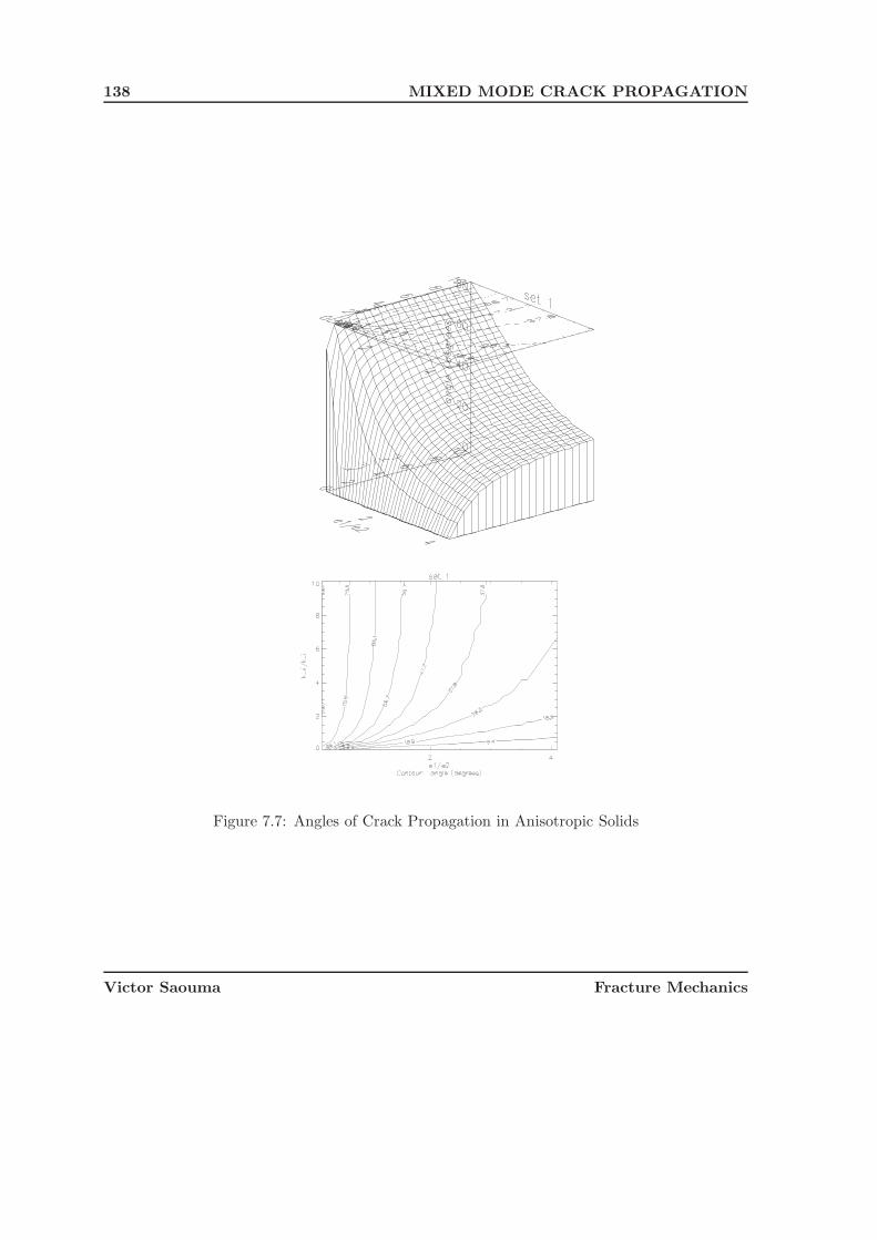
138 MIXED MODE CRACK PROPAGATION
Figure 7.7: Angles of Crack Propagation in Anisotropic Solids
Victor Saouma Fracture Mechanics

7.3 Extensions to Anisotropic Solids 139
Figure 7.8: Failure Surfaces for Cracked Anisotropic Solids
Victor Saouma Fracture Mechanics

140 MIXED MODE CRACK PROPAGATION
7.4 Interface Cracks
51 Interface crack propagation is rapidly gaining wide attention. Such crack growth is exceed-ingly important for composite materials, and can be extended to concrete/rock crack interfaces1.
52 A crack once initiated within an interface can either be stable or propagate in an unstablemanner. The unstable crack can propagate along the interface or kink into one of the materials.It can also branch out, that is, it can propagate along the interface and then kink. Whether acrack is forced to remain inside an interface or branch out, depends on the relative toughnessesof the interface and the ones of the adjacent materials. The criteria for an unstable crack topropagate or kink is described in this section. Also, if the crack has to kink, the angle of kinkwith respect to the interface will be considered.
53 The method presented is very similar to the one used for by the Maximum Energy Releaserate. We determine the energy release rate G0 if the crack were to propagate along the interface,the energy release rate G if the crack was to kink, and compare those two values with G0c andGc (material properties) respectively.
54 This section is introduced with the crack tip stresses at the bimaterial interface. As men-tioned earlier, the stress intensity factor for a bimaterial interface is complex, its physicaldimensions are briefly explained. These dimensions are used to obtain a relationship betweenthe homogeneous and the bimaterial stress intensity factors. With these relations, an analyti-cal expression for the energy release rate of the crack kinked into one of the materials is thenderived in terms of the energy release rate of the crack advance in the interface.
7.4.1 Crack Tip Fields
Ε
μ υ
θx
y
Ε
μ1 1 1
2 2 2
υ1
2
δ
δ x
y
Figure 7.9: Geometry and conventions of an interface crack, (Hutchinson and Suo 1992)
55 Considering the bimaterial interface crack in Fig. 7.9 for traction-free plane problems thenear-tip normal and shear stresses σyy and τxy, may conveniently be expressed in complex form
1This section was written by Kishen Chandra.
Victor Saouma Fracture Mechanics

7.4 Interface Cracks 141
(Hutchinson and Suo 1992)
σyy + iτxy =(K1 + iK2)r
iε√(2πr)
(7.53)
where i =√−1,K1 and K2 are components of the complex stress intensity factor K = K1+iK2
2, and ε is the oscillation index given by
ε =1
2πln[
1 − β
1 + β] (7.54)
where β is one of Dunders’ elastic mismatch parameters (Dunders 1969), which for plane strainis given by
β =μ1(1 − 2ν2) − μ2(1 − 2ν1)
2[μ1(1 − ν2) + μ2(1 − ν1)](7.55)
in which μ and ν are the shear modulus and Poisson’s ratio, respectively, and subscripts 1 and 2refer to the materials above and below the interface, respectively. Dunders defines an additionalmismatch parameter α:
α =E1 − E2
E1 + E2(7.56)
where E is the plane strain Young’s modulus, E = E/(1 − ν2).We note that β, α and ε vanishwhen the materials above and below the interface are identical. When ε �= 0, Equation 7.53shows that the stresses oscillate3heavily as the crack tip is approached (r → 0). Furthermore,the relative proportion of interfacial normal and shear stresses varies slowly with distance fromthe crack tip because of the factor riε. Thus K1 and K2 cannot be decoupled to represent theintensities of interfacial normal and shear stresses as in homogeneous fracture.
56 The crack flank displacements, for plane strain are given by (Hutchinson and Suo 1992,Carlsson and Prasad 1993)
δy + iδx =4√2π
(1/E1 + 1/E2)(K1 + iK2)
(1 + 2iε) cosh(πε)
√rriε (7.57)
where δy and δx are the opening and sliding displacements of two initially coincident points onthe crack surfaces behind the crack tip, as shown in Fig. 7.9. It may be noted from Eqn. 7.57that crack face interpenetration is implied when ε �= 0, as ε is an oscillatory term as shown inEqn. 7.54. The zone of contact, however, is generally exceedingly small compared to the cracktip plastic zone and may therefore be neglected (Hutchinson and Suo 1992).
57 The energy release rate, G, for extension of the crack along the interface, for plane strain isgiven by (Carlsson and Prasad 1993)
G =(1/E1 + 1/E2)(K
21 + K2
2 )
2 cosh2(πε)(7.58)
2Note that for interface cracks, it is customary to replace KI and KII by K1 and K2.3Recall Eq. ?? riλj = cos(λj log(r)) + i sin(λj log(r)).
Victor Saouma Fracture Mechanics

142 MIXED MODE CRACK PROPAGATION
58 The complications associated with nonzero ε and β may be circumvented by the approachto bimaterial interface crack problems proposed by He and Hutchinson (1989). They haveproposed to systematically take β = 0 in the analysis of fracture specimens and subsequentapplication of experimental data in failure predictions. Usually ε is very small and the effect ofnonzero β is of secondary importance. This will be discussed later in more detail.
7.4.2 Dimensions of Bimaterial Stress Intensity Factors
59 The tractions ahead of the crack tip, on the interface are given by Eqn. 7.53. Therefore Kwill necessarily have the dimensional form
K = K1 + iK2 =σ√
L
Liε(7.59)
where L is a length quantity such as crack length or ligament length, which would be discussedlater.
60 Alternatively for a homogeneous material, the dimensions of the stress intensity factor are
K = KI + iKII = σ√
L (7.60)
Thus it is clear that dimensionally, the homogeneous and bimaterial stress intensity factorsdiffer by L−iε.
61 Considering the kinked crack of length a as shown in Fig. 7.10, the singular stress field atits tip is the classical field with the conventional stress intensity factors, KI and KII such that,
σy′y′ + iτx′y′ =KI + iKII√
2πx′ (7.61)
ahead of the tip (x′ > 0, y′ = 0).
Ε
μ υ
θx
y
Ε
μ1 1 1
2 2 2
υ1
2
x
y
a
r
ω
|
|
Figure 7.10: Geometry of kinked Crack, (Hutchinson and Suo 1992)
Victor Saouma Fracture Mechanics
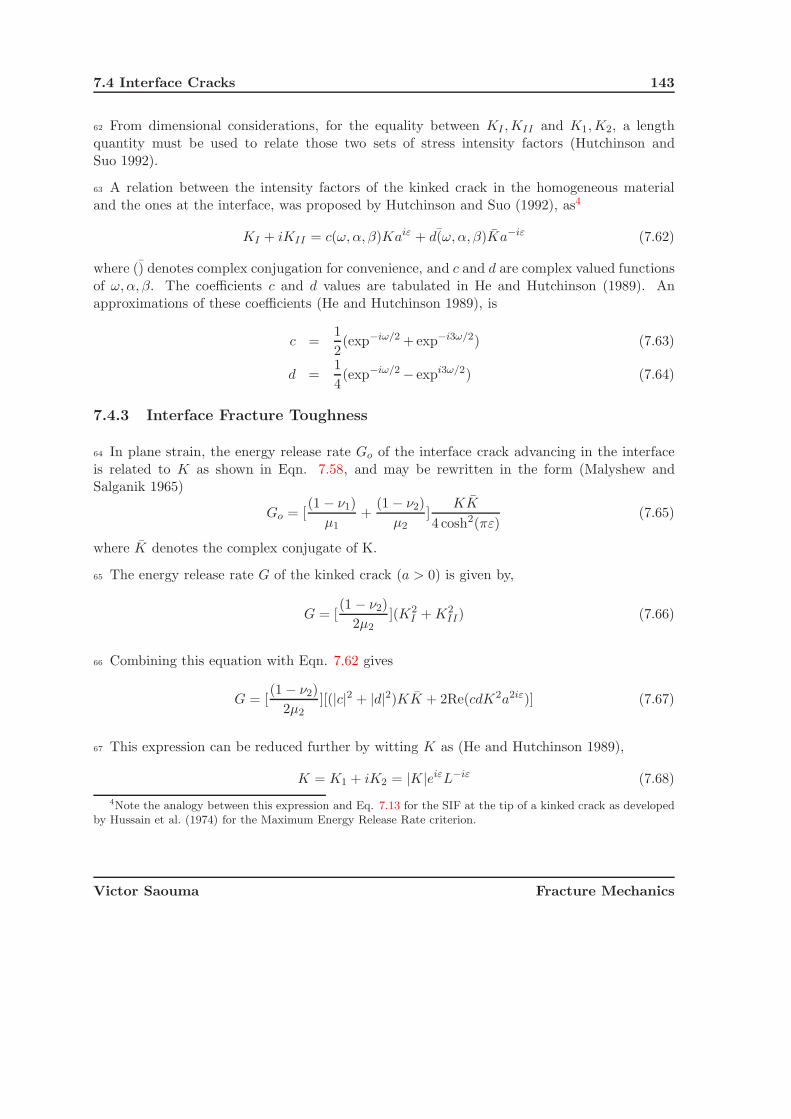
7.4 Interface Cracks 143
62 From dimensional considerations, for the equality between KI ,KII and K1,K2, a lengthquantity must be used to relate those two sets of stress intensity factors (Hutchinson andSuo 1992).
63 A relation between the intensity factors of the kinked crack in the homogeneous materialand the ones at the interface, was proposed by Hutchinson and Suo (1992), as4
KI + iKII = c(ω,α, β)Kaiε + d(ω,α, β)Ka−iε (7.62)
where () denotes complex conjugation for convenience, and c and d are complex valued functionsof ω,α, β. The coefficients c and d values are tabulated in He and Hutchinson (1989). Anapproximations of these coefficients (He and Hutchinson 1989), is
c =1
2(exp−iω/2 + exp−i3ω/2) (7.63)
d =1
4(exp−iω/2 − expi3ω/2) (7.64)
7.4.3 Interface Fracture Toughness
64 In plane strain, the energy release rate Go of the interface crack advancing in the interfaceis related to K as shown in Eqn. 7.58, and may be rewritten in the form (Malyshew andSalganik 1965)
Go = [(1 − ν1)
μ1+
(1 − ν2)
μ2]
KK
4 cosh2(πε)(7.65)
where K denotes the complex conjugate of K.
65 The energy release rate G of the kinked crack (a > 0) is given by,
G = [(1 − ν2)
2μ2](K2
I + K2II) (7.66)
66 Combining this equation with Eqn. 7.62 gives
G = [(1 − ν2)
2μ2][(|c|2 + |d|2)KK + 2Re(cdK2a2iε)] (7.67)
67 This expression can be reduced further by witting K as (He and Hutchinson 1989),
K = K1 + iK2 = |K|eiεL−iε (7.68)
4Note the analogy between this expression and Eq. 7.13 for the SIF at the tip of a kinked crack as developedby Hussain et al. (1974) for the Maximum Energy Release Rate criterion.
Victor Saouma Fracture Mechanics

144 MIXED MODE CRACK PROPAGATION
where by 7.59, L is the in-plane length quantity characterizing the specific interface crackproblem when a = 0. From Equations 7.65, 7.67 and 7.68 and using the real angular quantityγ as the measure of the loading combination,
G = q−2Go[|c|2 + |d|2 + 2Re(cd exp2iγ)] (7.69)
where
q = [(1 − β2)
(1 + α)]1/2 (7.70)
γ = γ + ε ln (a/L) (7.71)
γ = tan−1(K2/K1) (7.72)
68 When ε = 0, the stress intensity factors, KI and KII and G are independent of a. This isthe case of similar moduli across the interface (α = β = 0).
69 From Eqn. 7.54, ε is zero when β = 0 regardless the value of α. The oscillatory behavior ofthe interface crack fields and the a-dependence of G only appear when β �= 0. According to Heand Hutchinson (He and Hutchinson 1989), a sensible approach to gaining insight into interfacialfracture behavior, while avoiding complications associated with the oscillatory singularity, wouldbe to focus on material combinations with β = 0.
70 The interface crack with a = 0, suffers contact between the crack faces within some smalldistance from the tip, when β �= 0, therefore ε �= 0, as predicted by the elastic solutions ofthe crack fields (Comninou 1977, Rice 1988). Contact between crack faces is less likely for thekinked crack (a > 0;ω > 0) loaded such that KI and KII are positive, since this will open upthe crack at the kink. Nevertheless, contact will inevitably occur if ε �= 0 when a is sufficientlysmall compared to L (He and Hutchinson 1989).
a
L
G
G
G
G
L
U
*
Figure 7.11: Schematic variation of energy release rate with length of kinked segment of crackfor β �= 0, (Hutchinson and Suo 1992)
Victor Saouma Fracture Mechanics

7.4 Interface Cracks 145
71 The dependence of G on a for a given kink angle is shown qualitatively in Fig. 7.11 aspredicted by Eqn. 7.69 when ε �= 0. (He and Hutchinson 1989). When a/L becomes sufficientlysmall, G oscillates between a maximum GU and a minimum GL, which are found to be (Heand Hutchinson 1989)
GU = q−2Go[|c| + |d|]2 (7.73)
GL = q−2Go[|c| − |d|]2 (7.74)
and which depend on K1 and K2 only through Go. For values of a/L outside the oscillatoryrange G approaches G�, given by Eqn. 7.69, with γ = γ, i.e.,
G� = q−2Go[|c|2 + |d|2 + 2Re(cd exp2iγ)] (7.75)
G� coincides with G given by Eqn. 7.69, when ε = 0. Contact between the crack faces willinvalidate the prediction for G from Eqn. 7.69 when a/L is in the range where oscillatorybehavior occurs.
72 From a physical standpoint, G� should be relevant if there exists crack-like flaws emanatingfrom the interface whose lengths are greater than the zone of contact. That is, G� should berelevant in testing for kinking if the fracture process zone on the interface is large comparedto the contact zone of the idealized elastic solution. If it is not, then more attention must bepaid to the a-dependence of G and to the consideration of the contact. In any case G� shouldplay a prominent role in necessary conditions for a crack kinking out of an interface, becauseonce nucleated, the kinked crack has an energy release rate which rapidly approaches G� as itlengthens (He and Hutchinson 1989).
7.4.3.1 Interface Fracture Toughness when β = 0
73 When β = 0 (and thus ε = 0) Eqns. 7.53, 7.57 and 7.58, respectively become:
(σyy, τxy) =(K1,K2)√
(2πr)(7.76)
(δy , δx) =4√2π
[1
E1+
1
E2]√
r(K1,K2) (7.77)
G =1
2[
1
E1+
1
E2](K2
1 + K22 ) (7.78)
74 The interface stress intensity factors K1 and K2 play precisely the same role as their counter-parts in elastic fracture mechanics for homogeneous, isotropic solids. The mode 1 componentK1 is the amplitude of the singularity of the normal stresses ahead of the tip and the associatednormal separation of the crack flanks, while the mode 2 component, K2, governs the shearstress on the interface and the relative shearing displacement of the flanks.
Victor Saouma Fracture Mechanics

146 MIXED MODE CRACK PROPAGATION
75 When β = 0, the measure of the relative amount of mode 2 to mode 1 at the crack tip istaken as (Hutchinson and Suo 1992)
γ = tan−1(K2/K1) (7.79)
76 For the case of a finite crack in an infinite plane,
γ = tan−1(τ∞xy/σ∞
yy) (7.80)
77 The criteria for initiation of crack propagation along the interface when the crack tip isloaded in mixed mode by γ is
G = Γ(γ) (7.81)
78 Where Γ(γ) is the toughness of the interface and can be thought of as an effective surfaceenergy that depends on the mode of loading.
7.4.3.2 Interface Fracture Toughness when β �= 0
79 When β �= 0, the decoupling of the normal and shear components of stress on the interfaceand associated displacements behind the crack tip within the zone dominated by the singularity,does not occur. When β �= 0, the definitions of mode 1 and mode 2 require some modification.In addition, the traction-free line crack solution for the displacements implies that the crackfaces interpenetrate at some point behind the tip. Both of these features have caused conceptualdifficulties in the development of a mechanics of interfaces.
80 As noted by Rice (1988), a generalized interpretation of the mode measure is the mostimportant complication raised by the oscillatory singularity, and the approach explained hereis along the lines of one of his proposals (Hutchinson and Suo 1992). First, a definition of ameasure of the combination of mode is made that generalizes Eqn. 7.79.
81 Let L be a reference length whose choice will be discussed later. Noting the stress distribution(7.53) on the interface from the K-field, define γ as
γ = tan−1[Im(KLiε)
Re(KLiε)] (7.82)
where K = K1 + iK2 is the complex stress intensity factor.
82 For a choice of L within the zone of dominance of the K-field, Eqn. 7.82 is equivalent to
γ = tan−1[(τxy
σyy)r=L] (7.83)
83 Moreover, the definition reduces to Eqn. 7.79 when β = 0, since Liε = 1 when ε = 0. Whenε �= 0, a mode 1 crack is one with zero shear traction on the interface a distance L ahead of the
Victor Saouma Fracture Mechanics

7.4 Interface Cracks 147
tip, and a mode 2 crack has zero normal traction at that point. The measure of the proportionof ”mode 2” to ”mode 1” in the vicinity of the crack tip requires the specification of somelength quantity since the ratio of the shear traction to normal traction varies (very slowly) withdistance to the tip when β �= 0.
84 The choice of the reference length L is somewhat arbitrary, as explained by Hutchinson andSuo (1992). It is useful to distinguish between a choice based on an in-plane length L of thespecimen geometry, such as crack length, and a choice based on a material length scale, suchas the size of the fracture process zone or a plastic zone at fracture. The former is useful fordiscussing the mixed mode character of a bimaterial crack solution, independent of materialfracture behavior, while the latter is advantageous in interpreting mixed mode fracture data.
7.4.4 Crack Kinking Analysis
x
y
1
2a
ω
Gt
Figure 7.12: Conventions for a Crack Kinking out of an Interface, (Hutchinson and Suo 1992)
85 Fig. 7.12 shows a semi-infinite crack lying along the interface with its tip at the origin. Priorto kinking (a = 0), the parent crack is loaded with a complex interface stress intensity factorK = K1 + K2 with mixity γ defined by Eqn. 7.82 relative to some reference length L. Fordefiniteness, γ is taken to be positive with kinking down into material 2 as shown in Fig. 7.12.Negative γ-loadings with upward kinking can be analyzed by exchanging the materials, i.e.,switching the signs on α and β. Roughly speaking, α > 0 implies that material 1 is stiffer thanmaterial 2 and vice versa.
7.4.4.1 Numerical Results from He and Hutchinson
86 In their paper (He and Hutchinson 1989), the authors have carried out analysis of a crackkinking out of an interface with the aim of providing the crack mechanics needed to assesswhether an interface crack will tend to propagate in the interface or whether it will advanceby kinking out of the interface. The analysis provides the relationships among KI and KII forthe kinked crack and K1 and K2 for the interface crack as dependent on the kink angle ω and
Victor Saouma Fracture Mechanics

148 MIXED MODE CRACK PROPAGATION
the material moduli, as shown in Eqn. 7.62. The energy release rate of the kinked crack Gis also related to the energy release rate of the interface crack, Go, as shown in Eqn. 7.69. Aparametric study is conducted using these relations and the qualitative features which emergeare listed below.
• Bimaterial Problem with β = 0
1. The more compliant is the material into which the crack kinks, i.e. the larger is α,the larger is the energy release rate, with all factors being equal. Conversely, if thelower material into which the crack kinks is relatively stiffer (α < 0), then the energyrelease rate is reduced.
2. If the difference in the elastic moduli of the two materials are relatively large, theenergy release rate for a crack kinking into the stiff material can be less than theinterface release rate Go, for all combinations of loading. This suggests that un-der conditions when the compliant material is tough and the stiff material and theinterface are each relatively brittle with comparable toughnesses (as measured by acritical value of energy release rate), the crack will tend to be trapped in the interfacefor all loading combinations.
3. If the stiff material is even less tough than the interface, the crack may leave theinterface, but not necessarily by kinking. For example, when α = −0.75 (He andHutchinson 1989), the largest energy release rates occur when ω is small approachingzero, suggesting that the crack may smoothly curve out of the interface. Such a path,however, would not necessarily satisfy KII = 0.
4. From the plots (He and Hutchinson 1989) showing the direction ω corresponding tothe maximum energy release rate (i.e. where dG/dω = 0 or at ω = 0, whichevergives the larger G) as a function of the loading angle γ for various values of α, it isseen that for positive α i.e. for the crack kinking into the more compliant material,ω increases smoothly as γ increases from 0 to 90 deg.
5. When γ = 0, meaning K2 = 0, the direction of maximum energy release rate isgreater than zero for α > 0. This shows that the crack kinks into more compliantmaterial 2 with finite angle for γ = 0.
6. When α is negative, i.e. when material 2 is more stiffer than material 1, there existsa range of γ in the vicinity of γ = 0 for which the maximum occurs at ω = 0
7. For sufficiently negative α, the maximum of G also occurs at ω = 0 where γ is in thevicinity of 90 deg.
8. For α, more negative than -0.67, the maximum occurs at ω = 0 for all γ.
9. The direction ω corresponding to KII = 0 is sometimes suggested as an alternativeto ω as the kink direction. A comparison between ω and ω is shown in He andHutchinson (1989), for α = 0 and α = ±0.5. In the homogeneous case when α = 0,the difference between ω and ω is less than 1 deg. for nearly all γ except near γ = π/2where it becomes about 2 deg.
Victor Saouma Fracture Mechanics

7.4 Interface Cracks 149
10. The difference between the two directions is also very minor for α = ±0.5.
11. For more negative values of α than -0.5, the range of γ in which Gmax occurs atω = 0 becomes significant, while KII = 0 at values of ω near the local maximum ofG which occurs for ω between 45 deg. and 60 deg. depending on γ. In this range ofγ, ω and ω are significantly different.
• Bimaterial Problems with β �= 0
87 As discussed in connection with Eqn. 7.69, G is not independent of a when ε �= 0,but G approaches G� for all but very small a. Plots of G�/Go as a function of ω arefound in (He and Hutchinson 1989) for (α = 0.5, β = 0.25) and (α = −0.5, β = −0.25).Although the β values in these examples are quite large, the curves are quite similar tothwe curves obtained with the same values of α and with β = 0. Curves of ω associatedwith the maximum value of G� versus γ are also shown in (He and Hutchinson 1989),which indicate that the effect of β on ω is relatively weak.
7.4.4.2 Numerical Results Using Merlin
87 Merlin is a three dimensional finite element program having the capabilities of performingfracture mechanics based analysis. The Stern and Becker integral method has been implementedin it to determine the stress intensity factors for bimaterials. In order to check the accuracy ofthe numerical results with those of the analytical ones, the following analysis is performed.
88 A square centre-cracked plate of dimensions 20 X 20 inches, consisting of two isotropicmaterials is analyzed. The plate is subjected to tensile stresses in all directions. The crack, oflength 2 inches, is on the interface between the two materials. The geometry and the naturalboundary conditions are shown in Fig. 7.13, and the finite element mesh is shown in Fig. 7.14.This mesh was generated using the pre-processor developed for Merlin. Since the analyticalresults for this problem were available for plane stress condition in (Lin and Mar 1976), sevendifferent cases with varying moduli ratios were considered in this analyses. The material in theupper portion of the plate is identified as material 1 and the material in the lower portion isidentified as material 2. The elastic modulus E2 for material 2 was kept fixed at 1 psi and thepoisson’s ratio of material 1 was fixed at 0.3. The tensile stress in the y-direction, σyy in all thecases was 1 psi and in the x-direction, the tensile stress σxx for material 1 was fixed at 1 psi.σxx for material 2 was varied for different cases as tabulated in Table 7.1. Symmetry of theplate about the centreline perpendicular to the crack and the material interface is consideredin the finite element model.
89 It is worth mentioning at this point that the modulus of elasticity of concrete is in the range2× 106 − 4× 10⁶psi and for rock 5× 10⁵ − 10× 106psi. Generally in the case of dams the ratioof the modulus of elasticity of concrete to that of rock is somewhere around 3.
90 The stress intensity factors K1 and K25 was obtained in (Lin and Mar 1976) using the
5K1 and K2 as explained earlier are the real and imaginary parts of the complex stress intensity factor
Victor Saouma Fracture Mechanics

150 MIXED MODE CRACK PROPAGATION
Material # 1
Material # 2
σ
σ
σ
σ
xx1
xx2
yy
yy
10"
20"
1"
Notch
Figure 7.13: Geometry and Boundary Conditions of the Plate Analyzed,
Figure 7.14: Finite Element Mesh of the Plate Analyzed,
Victor Saouma Fracture Mechanics
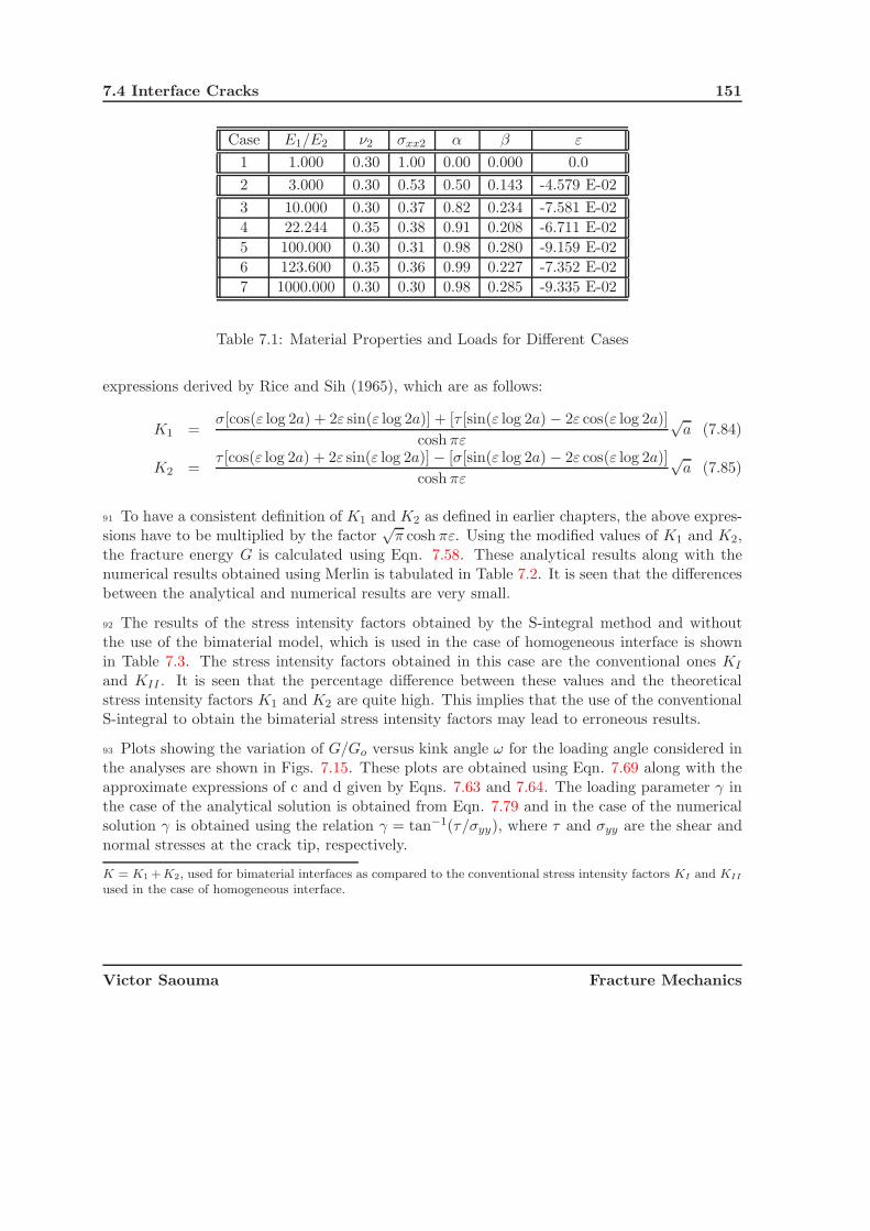
7.4 Interface Cracks 151
Case E1/E2 ν2 σxx2 α β ε
1 1.000 0.30 1.00 0.00 0.000 0.0
2 3.000 0.30 0.53 0.50 0.143 -4.579 E-02
3 10.000 0.30 0.37 0.82 0.234 -7.581 E-02
4 22.244 0.35 0.38 0.91 0.208 -6.711 E-02
5 100.000 0.30 0.31 0.98 0.280 -9.159 E-02
6 123.600 0.35 0.36 0.99 0.227 -7.352 E-02
7 1000.000 0.30 0.30 0.98 0.285 -9.335 E-02
Table 7.1: Material Properties and Loads for Different Cases
expressions derived by Rice and Sih (1965), which are as follows:
K1 =σ[cos(ε log 2a) + 2ε sin(ε log 2a)] + [τ [sin(ε log 2a) − 2ε cos(ε log 2a)]
cosh πε
√a (7.84)
K2 =τ [cos(ε log 2a) + 2ε sin(ε log 2a)] − [σ[sin(ε log 2a) − 2ε cos(ε log 2a)]
cosh πε
√a (7.85)
91 To have a consistent definition of K1 and K2 as defined in earlier chapters, the above expres-sions have to be multiplied by the factor
√π cosh πε. Using the modified values of K1 and K2,
the fracture energy G is calculated using Eqn. 7.58. These analytical results along with thenumerical results obtained using Merlin is tabulated in Table 7.2. It is seen that the differencesbetween the analytical and numerical results are very small.
92 The results of the stress intensity factors obtained by the S-integral method and withoutthe use of the bimaterial model, which is used in the case of homogeneous interface is shownin Table 7.3. The stress intensity factors obtained in this case are the conventional ones KI
and KII . It is seen that the percentage difference between these values and the theoreticalstress intensity factors K1 and K2 are quite high. This implies that the use of the conventionalS-integral to obtain the bimaterial stress intensity factors may lead to erroneous results.
93 Plots showing the variation of G/Go versus kink angle ω for the loading angle considered inthe analyses are shown in Figs. 7.15. These plots are obtained using Eqn. 7.69 along with theapproximate expressions of c and d given by Eqns. 7.63 and 7.64. The loading parameter γ inthe case of the analytical solution is obtained from Eqn. 7.79 and in the case of the numericalsolution γ is obtained using the relation γ = tan−1(τ/σyy), where τ and σyy are the shear andnormal stresses at the crack tip, respectively.
K = K1 +K2, used for bimaterial interfaces as compared to the conventional stress intensity factors KI and KII
used in the case of homogeneous interface.
Victor Saouma Fracture Mechanics

152 MIXED MODE CRACK PROPAGATION
Case Analytical Numerical % difference
K1 K2 K1 K2 K1 K2
1 1.773 0.00 1.841 0.15 4.01 —
2 1.770 0.13 1.872 0.16 5.76 20.77
3 1.765 0.21 1.872 0.22 5.76 0.0
4 1.750 0.22 1.869 0.23 6.80 0.0
5 1.760 0.27 1.875 0.26 6.82 0.0
6 1.747 0.24 1.871 0.24 6.86 0.0
7 1.761 0.26 1.873 0.26 6.25 0.0
Table 7.2: Analytical and Numerical Results
Case Analytical Numerical % difference
K1 K2 KI KII K1 K2
1 1.773 0.00 1.386 0.2408 22.00 —
2 1.770 0.13 1.525 0.0047 13.70 96
3 1.765 0.21 1.352 0.0158 23.40 93
4 1.750 0.22 1.312 0.0083 25.02 96
5 1.760 0.27 1.275 0.0072 27.60 97
6 1.747 0.24 1.281 0.0041 26.70 98
7 1.761 0.26 1.265 0.0057 28.10 98
Table 7.3: Numerical Results using S-integral without the bimaterial model
Victor Saouma Fracture Mechanics

7.4 Interface Cracks 153
0 45 90 135Kink Angle ω (deg.)
0.0
0.2
0.4
0.6
0.8
1.0
1.2
G/G
o
E1/E2 = 22.25, ν1 = 0.3, ν2 = 0.35
Analytical γ = 7.1 deg.Numerical γ = 12.5 deg.
0 45 90 135KInk Angle ω (deg.)
0.0
0.2
0.4
0.6
0.8
1.0
1.2
G/G
o
E1/E2 = 3.0, ν1 = 0.3, ν2 = 0.3
Analytical γ = 4.2 deg.Numerical γ = 3.4 deg.
0 45 90 135Kink Angle ω (deg.)
0.0
0.2
0.4
0.6
0.8
1.0
1.2
G/G
o
E1/E2 = 100.0, ν1 = 0.3, ν2 = 0.3
Analytical γ = 8.3 deg.Numerical γ = 15.7 deg.
0 45 90 135Kink Angle ω (deg)
0.0
0.2
0.4
0.6
0.8
1.0
1.2
G/G
o
E1/E2 = 10.0, ν1= 0.3, ν2 = 0.3
Analytical γ = 6.9 deg.Numerical γ = 12.5 deg.
0.5
1.0
0 45 90 135KInk Angle ω (deg.)
0.0
0.2
0.4
0.6
0.8
1.0
1.2
G/G
o
E1/E2 = 123.6, ν1 = 0.3, ν2 = 0.35
Analytical γ = 7.7 deg.Numerical γ = 13.8 deg.
0.8
1.0
1.2
o
E1/E2 = 100.0, ν1 = 0.3, ν2 = 0.3
0 45 90 135Kink Angle ω (deg)
0.0
0.2
0.4
0.6
0.8
1.0
1.2
G/G
o
E1/E2 = 1000.0, ν1= 0.3, ν2 = 0.3
Analytical γ = 8.5 deg.Numerical γ = 16.1 deg.
Victor Saouma Fracture Mechanics

154 MIXED MODE CRACK PROPAGATION
7.4.5 Summary
94 The results for the kinked crack can be used to access whether an interface crack will prop-agate in the interface or whether it will kink out of the interface.
LetGoc = critical fracture energy of the interface,Gic = critical fracture energy of material i,Gmax = maximum energy release rate in material i
1. The condition for propagation in the interface is Go = Goc and that for propagating inany one of the two materials is G = Gic.
2. Conditions for crack kinking and propagation:
•(
Gmax < Gic
Go < Goc
)no crack propagation.
•(
Gmax ≥ Gic
Go < Goc
)crack kinks in material i .
•(
Gmax < Gic
Go ≥ Goc
)crack propagates along the interface.
•(
Gmax ≥ Gic
Go ≥ Goc
)crack kinks and propagates i.e. the crack branches.
3. If Gic is sufficiently large when compared to Goc, the crack will never kink into materiali.
4. When Gic is comparable to Goc, there will still be a loading range, i.e. 0 ≤ γ ≤ γmax,such that the crack stays in the interface, while for γ > γmax, the interface crack will kinkinto material i.
5. When the fractured interface has some roughness, Goc might depend on the loading pa-rameter γ. Hence the level of Gic required to prevent kinking out of the interface willdepend on the interface toughness Goc at the loading angle γ applied.
6. When there is no dissimilarity in the elastic properties of the materials across the interface,the direction of kinking associated with the maximum energy release rate and with KII =0 are virtually the same.
7. When the crack has penetrated well into material i, a criterion based on KII = 0 isexpected to hold.
8. Crack deflection analysis based on the crack kinking and maximum principal stress the-ories indicate that global mode I loading generally favors interfacial crack propagation.For global mode II loading, crack deflection into the core is a likely scenario because offavorable conditions and large crack driving force.
Victor Saouma Fracture Mechanics

7.4 Interface Cracks 155
9. A choice of criterion for the initial kinking step will have to be guided by experiment.
Victor Saouma Fracture Mechanics

156 MIXED MODE CRACK PROPAGATION
Victor Saouma Fracture Mechanics
Part III
ELASTO PLASTIC FRACTUREMECHANICS


Chapter 8
PLASTIC ZONE SIZES
1 it was shown in chapter 3 that, under linear elastic fracture mechanics assumptions, the stressat the crack tip is theoretically infinite. Clearly, all materials have a finite strength, thus therewill always be a small plastified zone around the crack tip.
2 If this zone is small compared to the crack size, then our linear elastic assumptions are correct;if not, LEFM is not applicable (thus it would be incorrect to use a K or G criterion) and anonlinear model must be used. This “damaged” zone is referred to as a plastic zone for metals,and a fracture process zone for cementitious materials and ceramics.
3 Thus there are two important issues associated with nonlinear fracture:
1. What is the size of the plastic or process zone?
2. What are the criteria for crack growth?
4 This chapter will answer the first question by focusing on metals1, whereas the next chapterwill develop criterions for crack growth.
5 The evaluation of the plastic zone for plastified materials can be determined through variouslevels of approximations:
1. Uniaxial stress criteria
(a) first order approximation
(b) second order approximation (Irwin)
(c) Dugdale’s model
2. Multiaxial yield criteria
Each one of them will be separately reviewed.
1Due to the intrinsically different behavior of concrete compared to metals, estimates of the fracture processzone will be separately discussed.

160 PLASTIC ZONE SIZES
8.1 Uniaxial Stress Criteria
6 First we shall examine criteria in which only the uniaxial stress state (σyy normal to theecrack axis) and we shall consider three models of increasing complexities.
8.1.1 First-Order Approximation.
7 The simplest estimate of the size of a process zone is obtained by equating σy (Eq. 3.52-b)
σyy =KI
(2πr)12
cosθ
2
[1 + sin
θ
2sin
3θ
2
](8.1)
to the yield stress σyld for θ = 0, Fig. 8.1
σyy =KI√2πr∗p
= σyld (8.2)
or
r∗p =1
2π
K2I
σ2yld
=a
2
(σ
σyld
)2
(8.3)
Figure 8.1: First-Order Approximation of the Plastic Zone
8.1.2 Second-Order Approximation (Irwin)
8 In 1960, Irwin (Irwin 1960) developed a second-order approximation for the plastic zone basedon the stress redistribution occurring at the crack tip. In the first model, we started with astress distribution which satisfied equilibrium, and “cut down” all stresses exceeding σyld. As aresult equilibrium was no longer satisfied. In this model the force (area under the stress curve)
Victor Saouma Fracture Mechanics

8.1 Uniaxial Stress Criteria 161
Figure 8.2: Second-Order Approximation of the Plastic Zone
which was “eliminated” is simply redistributed to satisfy equilibrium requirements. Hence, withreference to Fig. 8.2, we have:
B = σyldδ (8.4)
A =
∫ r∗p
0σdr − σyldr
∗p
=
∫ r∗p
0
K√2πr
dr − σyldr∗p
=
∫ r∗p
0
σ√
πa√2πr
dr − σyldr∗p
=
∫ r∗p
0σ
√a
2r−
12 dr − σyldr
∗p
= σ
√a
22r
12 |r
∗
p
0 −σyldr∗p
= σ√
2ar∗p − σyldr∗p (8.5)
9 Equating A to B we obtain:
σ√
2ar∗p − σyldr∗p = σyldδ
σyld(δ + r∗p) = σ√
2ar∗p
(δ + r∗p)2 =
2aσ2
σ2yld
r∗p (8.6)
Victor Saouma Fracture Mechanics
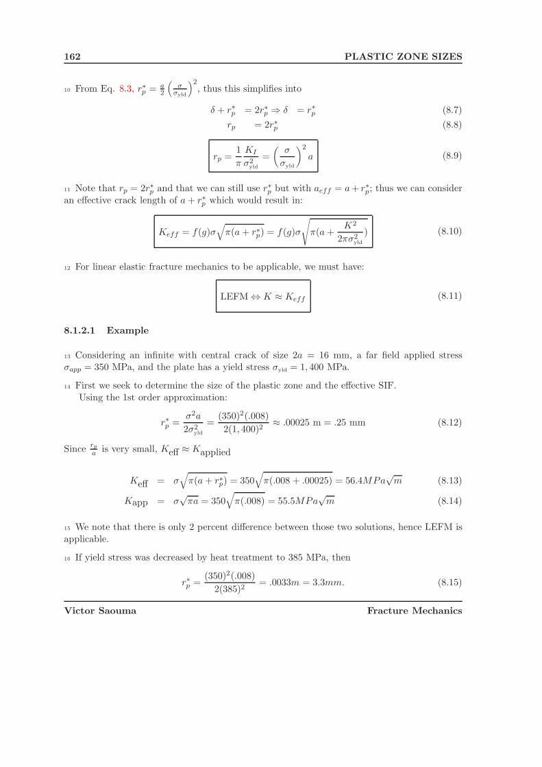
162 PLASTIC ZONE SIZES
10 From Eq. 8.3, r∗p = a2
(σ
σyld
)2, thus this simplifies into
δ + r∗p = 2r∗p ⇒ δ = r∗p (8.7)
rp = 2r∗p (8.8)
rp =1
π
KI
σ2yld
=
(σ
σyld
)2
a (8.9)
11 Note that rp = 2r∗p and that we can still use r∗p but with aeff = a + r∗p; thus we can consideran effective crack length of a + r∗p which would result in:
Keff = f(g)σ√
π(a + r∗p) = f(g)σ
√π(a +
K2
2πσ2yld
) (8.10)
12 For linear elastic fracture mechanics to be applicable, we must have:
LEFM ⇔ K ≈ Keff (8.11)
8.1.2.1 Example
13 Considering an infinite with central crack of size 2a = 16 mm, a far field applied stressσapp = 350 MPa, and the plate has a yield stress σyld = 1, 400 MPa.
14 First we seek to determine the size of the plastic zone and the effective SIF.Using the 1st order approximation:
r∗p =σ2a
2σ2yld
=(350)2(.008)
2(1, 400)2≈ .00025 m = .25 mm (8.12)
Since rp
a is very small, Keff ≈ Kapplied
Keff = σ√
π(a + r∗p) = 350√
π(.008 + .00025) = 56.4MPa√
m (8.13)
Kapp = σ√
πa = 350√
π(.008) = 55.5MPa√
m (8.14)
15 We note that there is only 2 percent difference between those two solutions, hence LEFM isapplicable.
16 If yield stress was decreased by heat treatment to 385 MPa, then
r∗p =(350)2(.008)
2(385)2= .0033m = 3.3mm. (8.15)
Victor Saouma Fracture Mechanics

8.1 Uniaxial Stress Criteria 163
andKeff = 350
√π(.008 + .0033) = 66MPa
√m (8.16)
and in this case LEFM may no longer be applicable.
8.1.3 Dugdale’s Model.
17 Dugdale (Dugdale 1960) assumed that the actual physical crack of length 2a is replaced bya total effective crack of length 2c, where c = a + ρ, Fig. 8.3, such that:
1. A constant stress σyld is applied over ρ where a < x < c causing (a negative) Kρ.
2. c is selected in such a manner that∑
K = 0 or Kremote = −Kρ.
Figure 8.3: Dugdale’s Model
18 The solution to this model is found by first considering a point load P applied at a distancex from the crack center, as in Fig. 8.4, where the stress intensity factors are given by:
KA = P√πa
√a+xa−x
KB = P√πa
√a−xa+x (8.17)
Victor Saouma Fracture Mechanics

164 PLASTIC ZONE SIZES
Figure 8.4: Point Load on a Crack
19 Assuming dP = σylddx, and replacing in the above equations, we obtain:
Kρ =σyld√πa
∫ c
a
{√a + x
a − x+
√a − x
a + x
}dx (8.18)
20 Integration of this equation results in
Kρ = 2σy
√c
πarccos
a
c(8.19)
21 On the other hand, the stress intensity caused by the remote far field stress is given by:
Kremote = σ√
πc (8.20)
Equating Eq. 8.20 with Eq. 8.19 and solving, we obtain:
a
c= cos
(π
2
σ
σyld
)(8.21)
22 From Eq. 8.21, we observe
1. As σ → σyld,ac → 0, or ρ → ∞, Fig. 8.5
2. Using the Cosine Taylor’s expansion on Eq. 8.21, as σσyld
→ 0, we can rewrite:
a
c=
a
a + ρ= 1 − 1
2!
(πσ
2σyld
)2
+1
4!
(πσ
2σyld
)4
− 1
6!
(πσ
2σyld
)6
(8.22)
Neglecting all but the first two terms and solving for ρ
ρ =π2
8
(σ
σyld
)2
a =π
8
KI
σ2yld
(8.23)
Victor Saouma Fracture Mechanics

8.2 Multiaxial Yield Criteria 165
Figure 8.5: Effect of Plastic Zone Size on Dugdale’s Model
Eq. 8.23 should be compared with Eq. 8.9 (rp =(
σσyld
)2a) previously obtained.
23 Finally it should be mentioned that similar equations have been derived by Barenblatt(Barenblatt 1962) on the basis of a linear stress distribution, see Fig. 8.6.
Figure 8.6: Barenblatt’s Model
8.2 Multiaxial Yield Criteria
24 All the previous models have restricted themselves to θ = 0 and have used uniaxial yieldcriteria, but the size of the plastic zone can be similarly derived from a multi-axial yield criterion.
25 The principal stresses at a point with respect to the crack tip are given by:
σ1,2 =σx + σy
2±√(
σx − σy
2
)2
+ τ2xy (8.24)
Victor Saouma Fracture Mechanics

166 PLASTIC ZONE SIZES
where the stresses were obtained in Eq. 3.52-a, 3.52-b, and 3.52-c
σ1 =KI√2πr
cosθ
2
[1 + sin
θ
2
](8.25)
σ2 =KI√2πr
cosθ
2
[1 − sin
θ
2
](8.26)
σ3 = ν(σ1 + σ2) (8.27)
for plane strain, orσ3 = 0 (8.28)
for plane stress.
26 With those stress expressions, any yield criteria could be used. Using the von Mises criteria,we would obtain:
σe =1√2
[(σ1 − σ2)
2 + (σ2 − σ3)2 + (σ3 − σ1)
2] 1
2(8.29)
and yielding would occur when σe reaches σyld. Substituting the principal stresses (with r = rp)into this equation and solving for rp yields
• For plane strain:
rp(θ) =1
4π
KI
σ2yld
[3
2sin2 θ + (1 − 2ν)2(1 + cos θ)
](8.30)
• For plane stress:
rp(θ) =1
4π
KI
σ2yld
[1 +
3
2sin2 θ + cos θ
](8.31)
27 For the Drucker-Prager model, and for different mixed mode ratios, the expected plastic (ormore appropriately process) zones are shown in Fig. 8.7.
28 In general, for the plastic zone sizes:
1. Different sizes would be obtained from alternative models (Tresca’s would be larger thanvon Mises’s).
2. The plastic zone for plane strain is much smaller than the one for plane stress (by a factorof (1 − 2ν)2).
3. Similar shapes could be derived if both KI and KII expressions were used.
4. This is only a first-order approximation, as no stress redistribution has been accountedfor.
Victor Saouma Fracture Mechanics
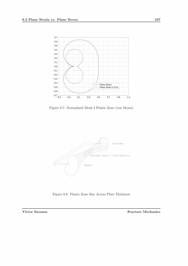
8.3 Plane Strain vs. Plane Stress 167
−0.3 −0.1 0.1 0.3 0.5 0.7 0.9 1.1−0.7
−0.6
−0.5
−0.4
−0.3
−0.2
−0.1
0.0
0.1
0.2
0.3
0.4
0.5
0.6
0.7
Plane StressPlane Strain (ν=0.3)
Figure 8.7: Normalized Mode I Plastic Zone (von Myses)
Figure 8.8: Plastic Zone Size Across Plate Thickness
Victor Saouma Fracture Mechanics

168 PLASTIC ZONE SIZES
8.3 Plane Strain vs. Plane Stress
29 Irrespective of a plate thickness, there is a gradual decrease in size of the plastic zone fromthe plate surface (plane stress) to the interior (plane strain), Fig. 8.8.
30 The ratio of the plastic zone size to the plate thicknessrp
B must be much smaller than unityfor plane strain to prevail. It has been experimentally shown that this ratio should be less than0.025.
Plane Strain KIc ⇔ rp < .025B (8.32)
31 We also observe that since rp is proportional to(
KI
σyld
)2, the plate thickness should increase
as either the SIF increase or the yield stress decrease.
32 Furthermore, the different stress fields present at the tip of the crack under plane stress andplane strain will result in different deformation patterns. This is best explained in terms of theorientation of the planes of maximum shear stress for both cases, Fig. 8.9.
maxτ
σ
σ
σ σ
z
y
x
zx
σσy
τ
σ
τ
σσσx z y
maxτ
Plane Strain
σ
σ
Plane Stressz
x
y
Figure 8.9: Plastic Zone Size in Comparison with Plate Thickness; Plane Stress and PlaneStrain
Victor Saouma Fracture Mechanics
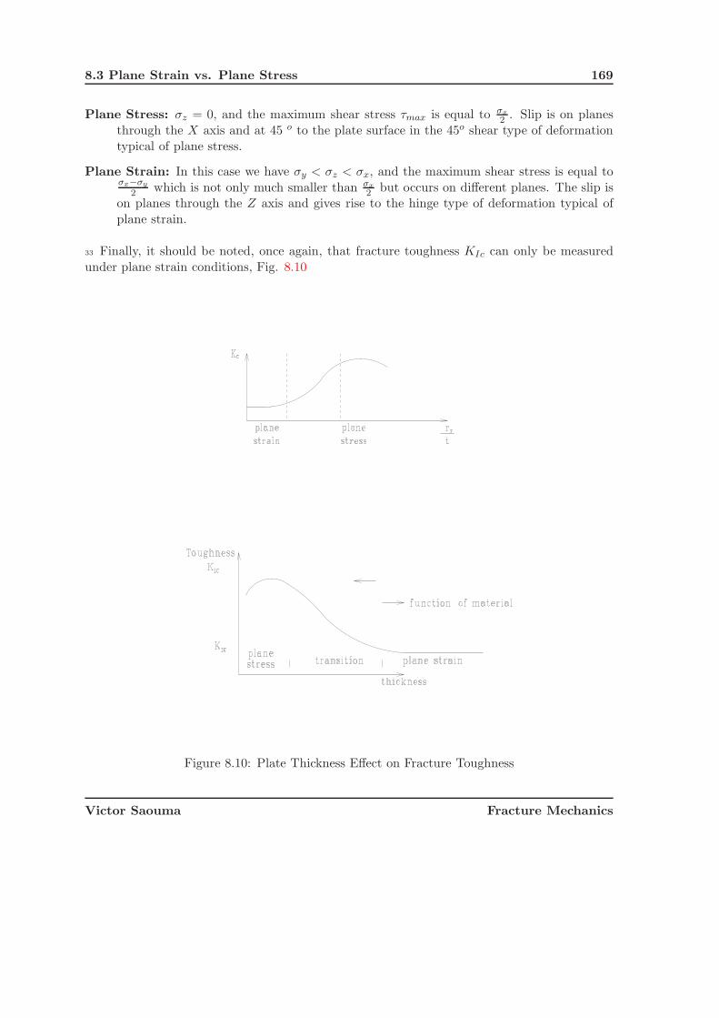
8.3 Plane Strain vs. Plane Stress 169
Plane Stress: σz = 0, and the maximum shear stress τmax is equal to σx
2 . Slip is on planesthrough the X axis and at 45 o to the plate surface in the 45o shear type of deformationtypical of plane stress.
Plane Strain: In this case we have σy < σz < σx, and the maximum shear stress is equal toσx−σy
2 which is not only much smaller than σx
2 but occurs on different planes. The slip ison planes through the Z axis and gives rise to the hinge type of deformation typical ofplane strain.
33 Finally, it should be noted, once again, that fracture toughness KIc can only be measuredunder plane strain conditions, Fig. 8.10
Figure 8.10: Plate Thickness Effect on Fracture Toughness
Victor Saouma Fracture Mechanics

170 PLASTIC ZONE SIZES
Victor Saouma Fracture Mechanics
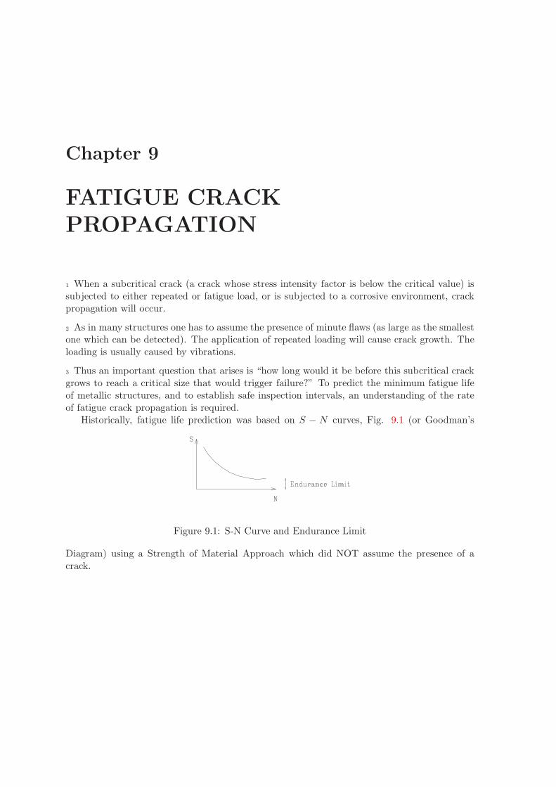
Chapter 9
FATIGUE CRACKPROPAGATION
1 When a subcritical crack (a crack whose stress intensity factor is below the critical value) issubjected to either repeated or fatigue load, or is subjected to a corrosive environment, crackpropagation will occur.
2 As in many structures one has to assume the presence of minute flaws (as large as the smallestone which can be detected). The application of repeated loading will cause crack growth. Theloading is usually caused by vibrations.
3 Thus an important question that arises is “how long would it be before this subcritical crackgrows to reach a critical size that would trigger failure?” To predict the minimum fatigue lifeof metallic structures, and to establish safe inspection intervals, an understanding of the rateof fatigue crack propagation is required.
Historically, fatigue life prediction was based on S − N curves, Fig. 9.1 (or Goodman’s
Figure 9.1: S-N Curve and Endurance Limit
Diagram) using a Strength of Material Approach which did NOT assume the presence of acrack.

172 FATIGUE CRACK PROPAGATION
9.1 Experimental Observation
4 If we start with a plate that has no crack and subject it to a series of repeated loading, Fig.9.2 between σmin and σmax, we would observe three distinct stages, Fig. 9.3
Figure 9.2: Repeated Load on a Plate
Figure 9.3: Stages of Fatigue Crack Growth
1. Stage 1 : Micro coalescence of voids and formation of microcracks. This stage is difficultto capture and is most appropriately investigated by metallurgists or material scientists,and compared to stage II and III it is by far the longest.
2. Stage II : Now a micro crack of finite size was formed, its SIF’well belowKIc, (K << KIc),and crack growth occurs after each cycle of loading.
3. Stage III : Crack has reached a size a such that a = ac, thus rapid unstable crack growthoccurs.
5 Thus we shall primarily be concerned by stage II.
9.2 Fatigue Laws Under Constant Amplitude Loading
6 On the basis of the above it is evident that we shall be concerned with stage II only. Fur-thermore, fatigue crack growth can take place under:
1. Constant amplitude loading (good for testing)
Victor Saouma Fracture Mechanics

9.2 Fatigue Laws Under Constant Amplitude Loading 173
2. Variable amplitude loading (in practice)
7 Empirical mathematical relationships which require the knowledge of the stress intensityfactors (SIF), have been established to describe the crack growth rate. Models of increasingcomplexity have been proposed.
8 All of these relationships indicate that the number of cycles N required to extend a crack bya given length is proportional to the effective stress intensity factor range ΔK raised to a powern (typically varying between 2 and 9).
9.2.1 Paris Model
9 The first fracture mechanics-based model for fatigue crack growth was presented by Paris(Paris and Erdogan 1963) in the early ’60s. It is important to recognize that it is an empiricallaw based on experimental observations. Most other empirical fatigue laws can be consideredas direct extensions, or refinements of this one, given by
da
dN= C (ΔK)n (9.1)
which is a straight line on a log-log plot of dadN
vs ΔK, and
ΔK = Kmax − Kmin = (σmax − σmin)f(g)√
πa (9.2)
a is the crack length; N the number of load cycles; C the intercept of line along dadN
and is of
the order of 10−6 and has units of length/cycle; and n is the slope of the line and ranges from2 to 10. C and n are experimentally determined.
10 Equation 9.1 can be rewritten as :
ΔN =Δa
C [ΔK(a)]n(9.3)
or
N =
∫dN =
∫ af
ai
da
C [ΔK(a)]n(9.4)
11 Thus it is apparent that a small error in the SIF calculations would be magnified greatlyas n ranges from 2 to 6. Because of the sensitivity of N upon ΔK, it is essential to properlydetermine the numerical values of the stress intensity factors.
12 However, in most practical cases, the crack shape, boundary conditions, and load are in sucha combination that an analytical solution for the SIF does not exist and large approximationerrors have to be accepted. Unfortunately, analytical expressions for K are available for only few
Victor Saouma Fracture Mechanics
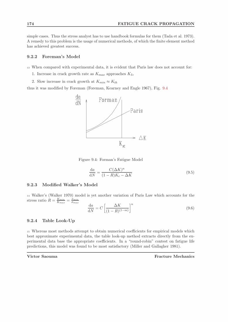
174 FATIGUE CRACK PROPAGATION
simple cases. Thus the stress analyst has to use handbook formulas for them (Tada et al. 1973).A remedy to this problem is the usage of numerical methods, of which the finite element methodhas achieved greatest success.
9.2.2 Foreman’s Model
13 When compared with experimental data, it is evident that Paris law does not account for:
1. Increase in crack growth rate as Kmax approaches KIc
2. Slow increase in crack growth at Kmin ≈ Kth
thus it was modified by Foreman (Foreman, Kearney and Engle 1967), Fig. 9.4
Figure 9.4: Forman’s Fatigue Model
da
dN=
C(ΔK)n
(1 − R)Kc − ΔK(9.5)
9.2.3 Modified Walker’s Model
14 Walker’s (Walker 1970) model is yet another variation of Paris Law which accounts for thestress ratio R = Kmin
Kmax= σmin
σmax
da
dN= C
[ΔK
(1 − R)(1−m)
]n(9.6)
9.2.4 Table Look-Up
15 Whereas most methods attempt to obtain numerical coefficients for empirical models whichbest approximate experimental data, the table look-up method extracts directly from the ex-perimental data base the appropriate coefficients. In a “round-robin” contest on fatigue lifepredictions, this model was found to be most satisfactory (Miller and Gallagher 1981).
Victor Saouma Fracture Mechanics

9.2 Fatigue Laws Under Constant Amplitude Loading 175
16 This method is based on the availability of the information in the following table:
dadN
ΔK
R =-1 R = .1 R = .3 R = .4
17 For a given dadN
and R, ΔK is directly read (or rather interpolated) for available data.
9.2.5 Effective Stress Intensity Factor Range
18 All the empirical fatigue laws are written in terms of ΔKI; however, in general a crack willbe subjected to a mixed-mode loading resulting in both ΔKI and ΔKII. Thus to properly usea fatigue law, an effective stress intensity factor is sought.
19 One approach, consists in determining an effective stress intensity factor ΔKeff in termsof ΔKI and ΔKII, and the angle of crack growth θ0. In principle each of the above discussedmixed-mode theories could yield a separate expression for the effective stress intensity factor.
20 For the case of maximum circumferential stress theory, an effective stress intensity factor isgiven by (Broek 1986):
ΔKIeff = ΔKI cos3 θ0
2− 3
2ΔKII cos
θ0
2sin θ0 (9.7)
9.2.6 Examples
9.2.6.1 Example 1
An aircraft flight produces 10 gusts per flight (between take-off and landing). It has two flightsper day. Each gust has a σmax = 200 MPa and σmin = 50 MPa. The aircraft is made up ofaluminum which has R = 15 kJ/m2 E = 70 GPa C = 5 × 10⁻¹¹ m/cycle, and n = 3. Thesmallest detectable flaw is 4 mm. How long would it be before the crack will propagate to itscritical length?
Assuming K = σ√
πa and KIc =√
ER, then ac = K2c
σ2maxπ = ER
σ2maxπ or
ac =(70 × 109)(15 × 103)
(200 × 106)2π= 0.0084 m = 8.4 mm (9.8)
⇒ N =
∫ af
ai
da
C[ΔK(a)]n=
∫ af
ai
da
C (σmax − σmin)n︸ ︷︷ ︸(Δσ)n
((πa)12 )n
=
∫ 8.4×10⁻³
4×10⁻³
da
(5 × 10⁻¹¹)︸ ︷︷ ︸C
(200 − 50)3︸ ︷︷ ︸(Δσ)3
(πa)1.5︸ ︷︷ ︸((πa).5)3
= 1064
∫ .0084
.004a−1.5da
= −2128a−.5 |.0084.004 = 2128[− 1√.0084
+ 1√.004
]
= 10, 428 cycles
(9.9)
Victor Saouma Fracture Mechanics
176 FATIGUE CRACK PROPAGATION
thus the time t will be: t = (10,428) cycles × 110
flightcycle
×12
dayflight
× 130
monthday
≈ 17.38 month
≈ 1.5 years.If a longer lifetime is desired, then we can:
1. Employ a different material with higher KIc, so as to increase the critical crack length ac
at instability.
2. Reduce the maximum value of the stress σmax.
3. Reduce the stress range Δσ.
4. Improve the inspection so as to reduce the assumed initial crack length amin.
9.2.6.2 Example 2
21 Repeat the previous problem except that more sophisticated (and expensive) NDT equipmentis available with a resolution of .1 mm thus ai = .1mm
t = 2128[− 1√.0084
+ 1√.0001
] = 184, 583 cycles
t = 173810,428 (189, 583) = 316 months ≈ 26 years!
9.2.6.3 Example 3
Rolfe and Barsoum p.261-263.
9.3 Variable Amplitude Loading
9.3.1 No Load Interaction
22 Most Engineering structures are subjected to variable amplitude repeated loading, however,most experimental data is based on constant amplitude load test. Thus, the following questionsarise:
1. How do we put the two together?
2. Is there an interaction between high and low amplitude loading?
1. Root Mean Square Model (Barsoum)
da
dN= C(ΔKrms)
n (9.10)
ΔKrms =
√∑ki=1 ΔK2
i
n(9.11)
where ΔKrms is the square root of the mean of the squares of the individual stress intensityfactors cycles in a spectrum.
Victor Saouma Fracture Mechanics

9.3 Variable Amplitude Loading 177
2. Accurate “block by block” numerical integration of the fatigue law
Δa = C(ΔK)nΔN (9.12)
solve for a instead of N .
9.3.2 Load Interaction
9.3.2.1 Observation
23 Under aircraft flight simulation involving random load spectrum:
• High wind related gust load, NH
• Without high wind related gust load, NL
NH > NL, thus “Aircraft that logged some bad weather flight time could be expected to possessa longer service life than a plane having a better flight weather history.”
24 Is this correct? Why? Under which condition overload is damaging!
9.3.2.2 Retardation Models
25 Baseline fatigue data are derived under constant amplitude loading conditions, but manystructural components are subjected to variable amplitude loading. If interaction effects ofhigh and low loads did not exist in the sequence, it would be relatively easy to establish a crackgrowth curve by means of a cycle-by-cycle integration. However crack growth under variableamplitude cycling is largely complicated by interaction effects of high and low loads.
26 A high level load occurring in a sequence of low amplitude cycles significantly reduces therate of crack growth during the cycles applied subsequent to the overload. This phenomena iscalled Retardation, Fig. 9.5.
Figure 9.5: Retardation Effects on Fatigue Life
27 During loading, the material at the crack tip is plastically deformed and a tensile plasticzone is formed. Upon load release, the surrounding material is elastically unloaded and a partof the plastic zone experiences compressive stresses.
Victor Saouma Fracture Mechanics

178 FATIGUE CRACK PROPAGATION
28 The larger the load, the larger the zone of compressive stresses. If the load is repeated ina constant amplitude sense, there is no observable direct effect of the residual stresses on thecrack growth behavior; in essence, the process of growth is steady state.
29 Measurements have indicated, however, that the plastic deformations occurring at the cracktip remain as the crack propagates so that the crack surfaces open and close at non-zero (posi-tive) levels.
30 When the load history contains a mix of constant amplitude loads and discretely appliedhigher level loads, the patterns of residual stress and plastic deformation are perturbed. As thecrack propagates through this perturbed zone under the constant amplitude loading cycles, itgrows slower (the crack is retarded) than it would have if the perturbation had not occurred.After the crack has propagated through the perturbed zone, the crack growth rate returns toits typical steady-state level, Fig. 9.6.
Figure 9.6: Cause of Retardation in Fatigue Crack Growth
9.3.2.2.1 Wheeler’s Model
31 Wheeler (Wheeler 1972) defined a crack-growth retardation factor Cp:
da
dN retarded= Cp
(da
dN
)linear
(9.13)
Cp =
(rpi
aoL + rpoL − ai
)m
(9.14)
in which rpi is the current plastic zone size in the ith cycle under consideration, ai is the currentcrack size, rpoL is the plastic size generated by a previous higher load excursion, aoL is the cracksize at which the higher load excursion occurred, and m is an empirical constant, Fig. 9.7.
32 Thus there is retardation as long as the current plastic zone is contained within the previouslygenerated one.
9.3.2.2.2 Generalized Willenborg’s Model
Victor Saouma Fracture Mechanics

9.3 Variable Amplitude Loading 179
Figure 9.7: Yield Zone Due to Overload
33 In the generalized Willenborg model (Willenborg, Engle and Wood 1971), the stress intensityfactor KI is replaced by an effective one:
KeffI = KI − KR (9.15)
in which KR is equal to:
KR = φKwR (9.16)
φ =1 − Kmax,th
Kmax,i
soL − 1(9.17)
KR = KwR = KoL
max
√1 − ai − aoL
rpoL− Kmax,i (9.18)
and ai is the current crack size, aoL is the crack size at the occurrence of the overload, rpoL isthe yield zone produced by the overload, KoL
max is the maximum stress intensity of the overload,and Kmax,i is the maximum stress intensity for the current cycle.
34 This equation shows that retardation will occur until the crack has generated a plastic zonesize that reaches the boundary of the overload yield zone. At that time, ai − aoL = rpoL andthe reduction becomes zero.
35 Equation 9.15 indicates that the complete stress-intensity factor cycle, and therefore itsmaximum and minimum levels (Kmax,i and Kmin,i), are reduced by the same amount (KR).Thus, the retardation effect is sensed by the change in the effective stress ratio calculated from:
Reff =Keff
min,i
Keffmax,i
=Kmin,i − KR
Kmax,i − KR(9.19)
because the range in stress intensity factor is unchanged by the uniform reduction.
Victor Saouma Fracture Mechanics

180 FATIGUE CRACK PROPAGATION
36 Thus, for the ith load cycle, the crack growth increment Δai is:
Δai =da
dN= f(ΔK,Reff) (9.20)
37 In this model there are two empirical constants: Kmax,th, which is the threshold stressintensity factor level associated with zero fatigue crack growth rate, and SoL, which is theoverload (shut-off) ratio required to cause crack arrest for the given material.
Victor Saouma Fracture Mechanics

Chapter 10
CRACK TIP OPENINGDISPLACEMENTS
1 Within the assumptions and limitations of LEFM we have two valid (and equivalent) criteriafor crack propagation: 1) K vs KIc which is a local criteria based on the strength of the stresssingularity at the tip of the crack; and 2) G vs GIc (or R) which is a global criteria based onthe amount of energy released (or consumed) during a unit surface crack’s propagations.
2 In many cases it is found that LEFM based criteria is either: too conservative and expensiveas it does not account for plastification at the crack tip, and/or invalid based on calculationsof r∗p where LEFM assumptions are checked.
3 Thus, in those cases where LEFM is not applicable, an alternative criteria for crack growthin Elasto Plastic Fracture Mechanics (EPFM) is sought.
4 But first let us note the various stages of ductile fracture:
1. Blunting of an initially sharp crack. Under LEFM assumptions, the crack tip openingdisplacement (CTOD) is zero, however in elasto-plastic material due to blunting it isdifferent from zero, Fig. 10.1.
2. Crack initiation
3. Slow (stable) crack growth
4. Unstable crack growth
5 Again two approaches are currently in use, Table 10.1
1. a local criterion based on the crack tip opening displacement (CTOD).
2. a global criterion based on the quasi-strain energy release rate (J integral), JIC.

182 CRACK TIP OPENING DISPLACEMENTS
Figure 10.1: Crack Tip Opening Displacement, (Anderson 1995)
Local Vector Global Scalar
LEFM K GEPFM CTOD J
Table 10.1: Comparison of Various Models in LEFM and EPFM
6 Historically the CTOD was first proposed as a valid criteria for crack propagation on thebasis of Cotterell and Wells work in the early 60’s at the British Welding Institute. This hasformed the basis of current “R-6” specifications for ductile failure in the U.K.
7 Under LEFM the crack tip opening displacement is clearly zero. However, when the materialis allowed to yield, then the crack tip will blunt resulting in a non-zero crack tip openingdisplacement (CTOD).
8 References (Cottrell 1963) and (Wells 1963) have introduced the concept of the crack tipopening displacement to characterize elasto-plastic fracture. This criterion is still the oneprimarily used in the United Kingdom, whereas the J integral is more commonly used in theUnited States.
9 There are two approaches to determine the CTOD:
1. First-order approximation based on a fictitious crack.
2. Second-order approximation based on Dugdale’s model.
10.1 Derivation of CTOD
10.1.1 Irwin’s Solution
10 The vertical displacement of a point next to the crack tip due to mode I loading is given byEq. 3.52-f, Fig. 10.2
Victor Saouma Fracture Mechanics

10.1 Derivation of CTOD 183
Figure 10.2: Estimate of the Crack Tip Opening Displacement, (Anderson 1995)
v =KI
2μ
[r
2π
] 12
sinθ
2
[κ + 1 − 2 cos2 θ
2
](10.1)
11 If we substitute θ = ±π we obtain the upper and lower displacements of the crack face, anddue to symmetry their sum corresponds to the crack opening displacement. Hence the crackopening is given by
COD = 2v =κ + 1
μKI
√r
2π(10.2)
12 If we substitute the crack tip opening displacement a distance r∗p away from the crack tipusing Irwin’s plastic zone correction from Eq. 8.9
r∗p =1
2π
K2I
σ2yld
(10.3)
into Eq. 10.2 and using κ = 3−ν1+ν for plane stress, and recall that μ = E/2(1 + ν), we obtain
CTOD =4
π
K2I
Eσyld
(10.4)
10.1.2 Dugdale’s Solution
13 Using Dugdale’s solution, Kanninen (Kanninen 1984) has shown that the crack opening alongthe crack is given by1:
v(x) =2
π
aσyld
E
{log
∣∣∣∣∣√
c2 − a2 +√
c2 − x2
√c2 − a2 −
√c2 − x2
∣∣∣∣∣+ x
alog
∣∣∣∣∣x√
c2 − a2 + a√
c2 − x2
x√
c2 − a2 − a√
c2 − x2
∣∣∣∣∣}
(10.5)
for 0 ≤ x ≤ c. For x = a this reduces to
v(a) =4
π
aσyld
Elog
c
a(10.6)
1Derivation of this equation can be found on p. 203 of (Anderson 1995)
Victor Saouma Fracture Mechanics
184 CRACK TIP OPENING DISPLACEMENTS
14 Combining this equation with Dugdale’s solution for c from Eq. 8.21,
a
c= cos
π
2
σ
σyld
(10.7)
we would then obtain
CTOD = 2v =8
π
aσyld
Elog
[sec
π
2
σ
σyld
](10.8)
15 using the series expansion of log sec:
CTOD =8
π
aσyld
E
[1
2
(π
2
σ
σyld
)2
+1
12
(π
2
σ
σyld
)4
+ · · ·]
(10.9)
or
CTOD =K2
Eσyld
[1 +
π2
24
σ2
σ2yld
+ . . .
](10.10)
note that for small σσyld
, the CTOD can be approximated by CTOD = K2
Eσyld.
10.2 G-CTOD Relations
16 Recalling also that the energy release rate G is given by G = K2
E′ , we obtain the followingapproximate equation
CTOD =G
σyld
(10.11)
and its counterpart
CTODcr =R
σyld
(10.12)
Victor Saouma Fracture Mechanics
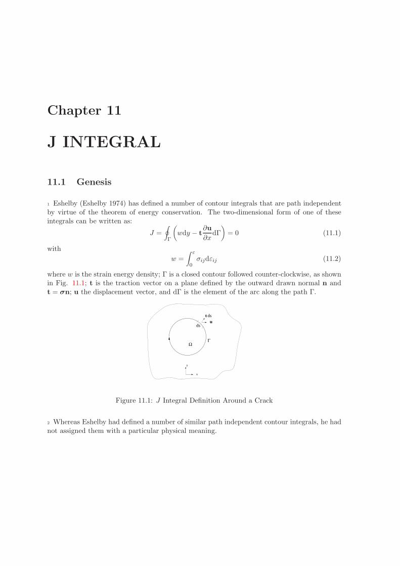
Chapter 11
J INTEGRAL
11.1 Genesis
1 Eshelby (Eshelby 1974) has defined a number of contour integrals that are path independentby virtue of the theorem of energy conservation. The two-dimensional form of one of theseintegrals can be written as:
J =
∮Γ
(wdy − t
∂u
∂xdΓ
)= 0 (11.1)
with
w =
∫ ε
0σijdεij (11.2)
where w is the strain energy density; Γ is a closed contour followed counter-clockwise, as shownin Fig. 11.1; t is the traction vector on a plane defined by the outward drawn normal n andt = σn; u the displacement vector, and dΓ is the element of the arc along the path Γ.
x
y
ΓΩ
ut ds
ds
Figure 11.1: J Integral Definition Around a Crack
2 Whereas Eshelby had defined a number of similar path independent contour integrals, he hadnot assigned them with a particular physical meaning.

186 J INTEGRAL
11.2 Proof of Path Independence
3 Before we establish the connection between Eshelby’s expression for J , and the energy releaserate J , we need to show that the former is indeed equal to zero for a closed path.
J =
∮Γ
(wdy − ti
∂ui
∂xdΓ
)(11.3)
and assuming Γ to be defined counterclockwise, then dx = −nydΓ, and dy = nxdΓ and ti =njσij where nx, ny and nj are direction cosines. Substituting
J =
∮Γ
(wnx − njσij
∂ui
∂x
)dΓ (11.4)
4 Invoking Green’s theorem ∮Γ
vinidΓ =
∫Ω
vi,idΩ (11.5)
we obtain
J =
∫Ω
[∂w
∂x− ∂
∂xj
(σij
∂ui
∂x
)]dxdy (11.6)
5 Applying the chain rule, the first term in the square bracket becomes
∂w
∂x=
∂w
∂εij
∂εij
∂x= σij
∂εij
∂x(11.7)
where the strain is given by Eq. ??
εij =1
2(ui,j + uj,i) (11.8)
6 Substituting for the first term
∂w
∂x=
1
2σij
[∂
∂x
(∂ui
∂xj
)+
∂
∂x
(∂uj
∂xi
)](11.9-a)
= σij∂
∂xj
(∂ui
∂x
)(11.9-b)
7 On the other hand, we have for the second term
∂
∂xj
(σij
∂ui
∂x
)= σij
∂
∂xj
(∂ui
∂x
)+
∂σij
∂xj︸ ︷︷ ︸0
∂ui
∂x(11.10-a)
Victor Saouma Fracture Mechanics

11.3 Nonlinear Elastic Energy Release Rate 187
8 Hence,∂w
∂x= σij
∂
∂xj
(∂ui
∂x
)(11.11)
which is identical to the second term of Eq. 11.6.
9 Thus the integrand of Eq. 11.3 vanishes and J = 0 for any closed contour.
10 Having shown that indeed J = 0, we will now exploit this to proove that around a crack, Jis non-zero and is independent of the path.
11 With reference to Fig. 11.2 if we consider the closed path Γ = Γ1 + Γ2 + Γ3 + Γ4 in which Γ1
and Γ3 are arbitrarily chosen contours. Obviously J = 0 over Γ in order to satisfy compatibilityconditions, provided that the stresses and displacement gradients are continuous. Along pathsΓ2 and Γ4, the traction vector ti = 0 and also dy = 0. Consequently, the contributions to Jfrom Γ2 and Γ4 vanish. Taking into account the difference sense of integration along pathsΓ1 and Γ3 we arrive at the conclusion that the values of J integrated over paths Γ1 and Γ3
are identical. Because these two paths were arbitrarily chosen, the path independence of J isassured.
Γ1Γ
ΓΓ3
2
4x
y
Figure 11.2: Closed Contour for Proof of J Path Independence
11.3 Nonlinear Elastic Energy Release Rate
12 Let us now establish the connection between the two previous interpretations of J , the onemathematically defined by Eshelby, and the one associated with the energy release rate (yetto be proven). We shall prove that when J is applied along a contour around a crack tip, itrepresents the change in potential energy for a virtual crack extension da. Two slightly differentderivations are presented.
Victor Saouma Fracture Mechanics

188 J INTEGRAL
11.3.1 Virtual Line Crack Extension
13 Considering a two-dimensional crack surrounded by a line Γ which encompasses an area Ω.Under quasi-static conditions, and in the absence of body forces, the potential energy is givenby
Π =
∫Ω
wdΩ︸ ︷︷ ︸U
−∮Γ
tiuidΓ︸ ︷︷ ︸W
(11.12)
14 For a virtual crack extension, the change in potential energy is
dΠ
da=
∫Ω
dw
dadΩ −
∮Γ
[ti
dui
da+ ui
dtida
]dΓ (11.13-a)
=
∫Ω
dw
dadΩ −
∮Γu︸︷︷︸0
[ti
dui
da+ ui
dtida
]dΓ −
∮Γt
⎡⎢⎢⎣ti
dui
da+ ui
dtida︸ ︷︷ ︸0
⎤⎥⎥⎦ dΓ (11.13-b)
15 We have decomposed the contour path into two parts, the first one with prescribed displace-ment (Γu) and a second one with prescribed traction (Γt). Since Γu is zero along the path, wemaintain a closed contour integral along Γt.
16 Furthermore, the second term inside the square bracket will be zero along Γt because thetraction is constant during crack growth.
17 For a crack extension, the coordinate axis also moves, Fig. 11.3. Thus we can write
Γx
y
Ω
Figure 11.3: Virtual Crack Extension Definition of J
d
da=
∂
∂a+
∂
∂x
∂x
∂a=
∂
∂a− ∂
∂x(11.14)
for a crack extension along a (∂x∂a = −1) with respect to the new coordinate system.
Victor Saouma Fracture Mechanics
11.3 Nonlinear Elastic Energy Release Rate 189
18 Substituting into Eq. 11.13-b
dΠ
da=
∫Ω
[∂w
∂a− ∂w
∂x
]dΩ −
∮Γt
ti
(∂ui
∂a− ∂ui
∂x
)dΓ (11.15)
19 We can also rewrite:
∂w
∂a=
∂w
∂εij
∂εij
∂a︸ ︷︷ ︸Eq. 11.7 = σij∂
∂xj
(∂ui
∂a
)︸ ︷︷ ︸
Eq. 11.9-b
(11.16)
20 But from the divergence theorem∮Γt
ti∂ui
∂adΓ =
∫Ω
σij∂
∂xj
(∂ui
∂a
)dΩ (11.17-a)
=
∫Ω
∂w
∂a(11.17-b)
Hence, from this Equation and Eq. 11.16, the first terms in each of the two integrals in Eq.11.15 cancel out, and we are left with
dΠ
da=
∮Γt
ti∂ui
∂xdΓ −
∫Ω
∂w
∂xdΩ (11.18)
21 We now apply the divergence theorem, multiply both sides by −1 and recalling that nxdΓ =dy
−dΠ
da=
∮Γt
(wnx − ti
∂ui
∂x
)dΓ
=∮Γt
(wdy − ti
∂ui
∂x dΓ) (11.19)
which is the same as Eq. 11.1. Henceforth, the J integral is equal to the energy release rate forlinear and nonlinear elastic material under quasi-static conditions.
11.3.2 †Virtual Volume Expansion
22 Following the brief preamble, let us thoroughly derive the expression for the J integral. Wewill derive an expression for the energy released during a unit surface crack extension based onthe following assumptions:
1. Homogeneous body
2. Linear or non-linear elastic solid
3. No inertia, or body forces; no initial stresses
Victor Saouma Fracture Mechanics

190 J INTEGRAL
4. No thermal loading
5. 2-D stress and deformation field
6. Plane stress or plane strain
7. Mode I loading
8. Stress free crack
23 Considering an arbitrary solid with both traction and displacement boundary conditions andan internal inclusion, Fig. 11.4
t
t , u
v
σ , ε
Γ
ΓΔ ΔΓ
ij ij
u
t
i i* *
o o
o
t
Figure 11.4: Arbitrary Solid with Internal Inclusion
Γ = Γt + Γu (11.20)
1. We define the initial boundary conditions as such
Surface initial boundary conditions:
(a) Displacements u0i on Γu
(b) Tractions t0i on Γt;
Internal stress and strain: σ0ij and ε0
ij
2. Due to ti and ui, the hole will grow and will have a new boundary, ΔΓ and volume ΔΩ.
3. However to prevent growth we will apply t∗i = σ0ijnj on ΔΓ in order to maintain initial
εij0 and σ0ij (Recall Irwin’s derivation of G).
Victor Saouma Fracture Mechanics
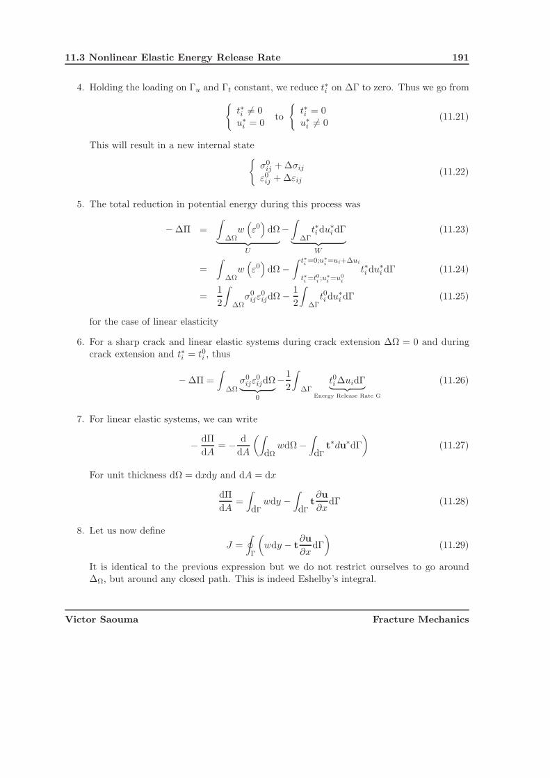
11.3 Nonlinear Elastic Energy Release Rate 191
4. Holding the loading on Γu and Γt constant, we reduce t∗i on ΔΓ to zero. Thus we go from{t∗i �= 0u∗
i = 0to
{t∗i = 0u∗
i �= 0(11.21)
This will result in a new internal state{σ0
ij + Δσij
ε0ij + Δεij
(11.22)
5. The total reduction in potential energy during this process was
− ΔΠ =
∫ΔΩ
w(ε0)
dΩ︸ ︷︷ ︸U
−∫
ΔΓt∗i du∗
i dΓ︸ ︷︷ ︸W
(11.23)
=
∫ΔΩ
w(ε0)
dΩ −∫ t∗
i=0;u∗
i=ui+Δui
t∗i=t0
i;u∗
i=u0
i
t∗i du∗i dΓ (11.24)
=1
2
∫ΔΩ
σ0ijε
0ijdΩ − 1
2
∫ΔΓ
t0i du∗i dΓ (11.25)
for the case of linear elasticity
6. For a sharp crack and linear elastic systems during crack extension ΔΩ = 0 and duringcrack extension and t∗i = t0i , thus
− ΔΠ =
∫ΔΩ
σ0ijε
0ijdΩ︸ ︷︷ ︸0
−1
2
∫ΔΓ
t0i ΔuidΓ︸ ︷︷ ︸Energy Release Rate G
(11.26)
7. For linear elastic systems, we can write
− dΠ
dA= − d
dA
(∫dΩ
wdΩ −∫dΓ
t∗du∗dΓ
)(11.27)
For unit thickness dΩ = dxdy and dA = dx
dΠ
dA=
∫dΓ
wdy −∫dΓ
t∂u
∂xdΓ (11.28)
8. Let us now define
J =
∮Γ
(wdy − t
∂u
∂xdΓ
)(11.29)
It is identical to the previous expression but we do not restrict ourselves to go aroundΔΩ, but around any closed path. This is indeed Eshelby’s integral.
Victor Saouma Fracture Mechanics

192 J INTEGRAL
9. We can decompose Γ = Γ1 +Γ2 where Γ1 is any external contour away from the crack tipand Γ2 to be identified with dΓ (increase in volume).
J = −∂Π
∂a=
∮r
(wdy − T
∂u
∂xdΓ
)(11.30)
J = −∂Π
∂a(11.31)
where Π is the potential energy. So for a linear elastic material −∂Π∂a = G, which implies
J = G (11.32)
24 Allowing Γ1 in Fig. 11.2 to shrink to an arbitrarily small contour Γc surrounding the cracktip, then the second term of Eq. 11.1 vanishes and
J =
∫Γc
wdy (11.33)
so that J is an averaged measure of the strain on the crack tip.
25 An arbitrarily small curve Γ may then be chosen surrounding the tip, so the integral maybe made to depend only on the crack tip singularity in the deformation field. The utility ofthe method rests in the fact that alternate choices of integration paths often permit a directevaluation of J .
26 In linear elastic analysis, and under pure mode I, Rice’s J can be used for the computationof stress intensity factor KI , as Eq. 11.1 yields
KI =
{√EJ1, (plane stress)√EJ1/(1 − ν2), (plane strain)
(11.34)
11.4 Nonlinear Energy Release Rate
27 Whereas LEFM is restricted to linear elastic materials, most metals have a nonlinear stress-strain curve. Fig. 11.5 illustrates the uniaxial stress-strain behavior of elastic-plastic andnonlinear elastic materials. Whereas the loading behavior of both materials is identical, theydiffer when they are unloaded. Thus, as long as there is no unloading, we can assume anonlinear elastic behavior, and the deformation theory of plasticity, which relates the totalstrains to stresses, is applicable.
28 For nonlinear elastic solids, we have already shown that J is the energy release rate innonlinear elastic materials:
J = −dΠ
da(11.35)
Victor Saouma Fracture Mechanics
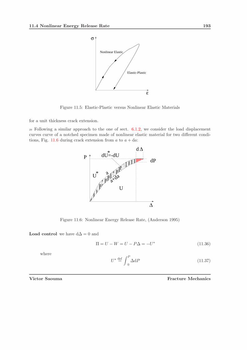
11.4 Nonlinear Energy Release Rate 193
Elastic-Plastic
Nonlinear Elastic
ε
σ
Figure 11.5: Elastic-Plastic versus Nonlinear Elastic Materials
for a unit thickness crack extension.
29 Following a similar approach to the one of sect. 6.1.2, we consider the load displacementcurves curve of a notched specimen made of nonlinear elastic material for two different condi-tions, Fig. 11.6 during crack extension from a to a + da:
*
d Δ*dU=-dU
U
U
dP
a+da
a
P
Δ
Figure 11.6: Nonlinear Energy Release Rate, (Anderson 1995)
Load control we have dΔ = 0 and
Π = U − W = U − PΔ = −U∗ (11.36)
where
U∗ def=
∫ P
0ΔdP (11.37)
Victor Saouma Fracture Mechanics
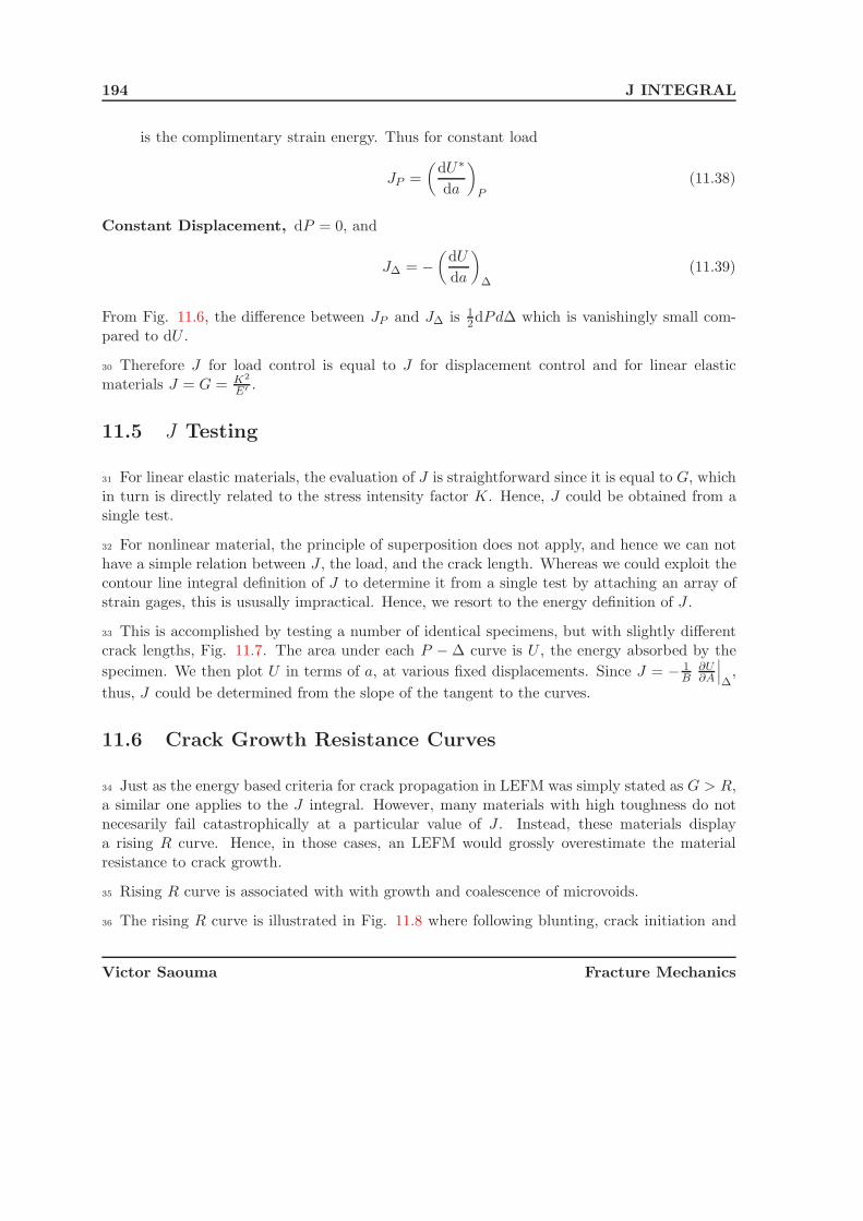
194 J INTEGRAL
is the complimentary strain energy. Thus for constant load
JP =
(dU∗
da
)P
(11.38)
Constant Displacement, dP = 0, and
JΔ = −(
dU
da
)Δ
(11.39)
From Fig. 11.6, the difference between JP and JΔ is 12dPdΔ which is vanishingly small com-
pared to dU .
30 Therefore J for load control is equal to J for displacement control and for linear elasticmaterials J = G = K2
E′ .
11.5 J Testing
31 For linear elastic materials, the evaluation of J is straightforward since it is equal to G, whichin turn is directly related to the stress intensity factor K. Hence, J could be obtained from asingle test.
32 For nonlinear material, the principle of superposition does not apply, and hence we can nothave a simple relation between J , the load, and the crack length. Whereas we could exploit thecontour line integral definition of J to determine it from a single test by attaching an array ofstrain gages, this is ususally impractical. Hence, we resort to the energy definition of J .
33 This is accomplished by testing a number of identical specimens, but with slightly differentcrack lengths, Fig. 11.7. The area under each P − Δ curve is U , the energy absorbed by the
specimen. We then plot U in terms of a, at various fixed displacements. Since J = − 1B
∂U∂A
∣∣∣Δ
,
thus, J could be determined from the slope of the tangent to the curves.
11.6 Crack Growth Resistance Curves
34 Just as the energy based criteria for crack propagation in LEFM was simply stated as G > R,a similar one applies to the J integral. However, many materials with high toughness do notnecesarily fail catastrophically at a particular value of J . Instead, these materials displaya rising R curve. Hence, in those cases, an LEFM would grossly overestimate the materialresistance to crack growth.
35 Rising R curve is associated with with growth and coalescence of microvoids.
36 The rising R curve is illustrated in Fig. 11.8 where following blunting, crack initiation and
Victor Saouma Fracture Mechanics
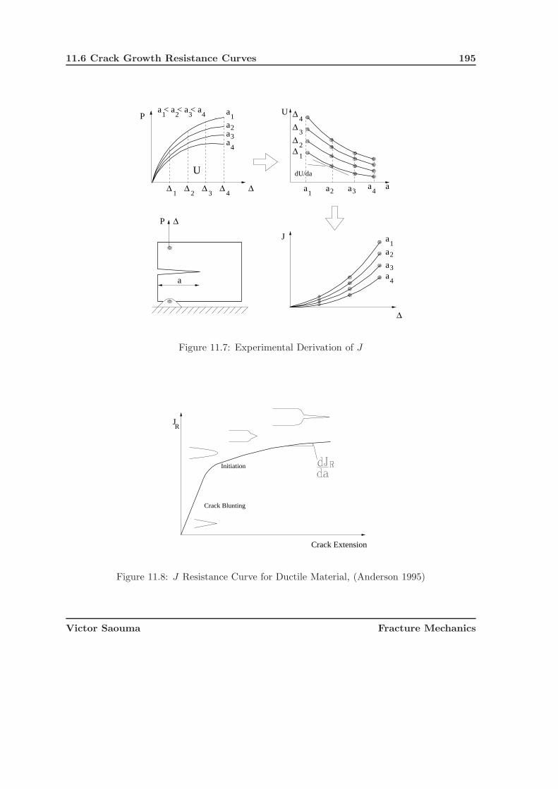
11.6 Crack Growth Resistance Curves 195
a
4a
3a
a
a1
a
4Δ1
1a
4321a < a < a < a
4a
3a
2
23
Δ
2Δ
1Δ
4Δ
3Δ
2Δ
1a2 a3
a4Δ
P
Δ
dU/da
U
a
Δ
J
a
P Δ
U
Figure 11.7: Experimental Derivation of J
JR
Crack Blunting
Initiation
Crack Extension
Figure 11.8: J Resistance Curve for Ductile Material, (Anderson 1995)
Victor Saouma Fracture Mechanics

196 J INTEGRAL
propagation occurs. An arbitrary definition of a critical J , JIc can be specified at the onset ofinitiation.
37 We define, a tearing modulus as
TR =E
σ2yld
dJR
da(11.40)
and the applied tearing modulus as
Tapp =E
σ2yld
dJ
da(11.41)
38 Hence, crack growth would occur if
J = JR
Tapp ≤ TR Stable crack growthTapp > TR Unstable crack growth
(11.42)
11.7 † Load Control versus Displacement Control
39 Crack propagation can occur under either load or displacement control. Whereas in bothcases J (and G) is the same, the rate of change of J depends on the loading condition.
40 Unstable crack propagation will occur if the rate of change of J exceeds the rate of changeof R.
41 The crack stability can be discussed within the context of the test stiffness (or its inverse thecomplinace). The total displacement is given by
ΔT = Δ + CmP (11.43)
where Cm is the compliance of the system.
42 Differentiating this equation yields
dΔt =
(∂Δ
∂a
)P
da +
(∂Δ
∂P
)adP + CmdP = 0 (11.44)
43 Similarly, we can take a similar derivative of J(a, P )
dJ =
(∂J
∂a
)P
da +
(∂J
∂P
)adP (11.45)
dividing both sides by da, and keeping ΔT constant(dJ
da
)ΔT
=
(∂J
∂a
)P
+
(∂J
∂P
)a
(dP
da
)ΔT
(11.46)
Victor Saouma Fracture Mechanics

11.8 Plastic Crack Tip Fields 197
44 Substituting(
∂P∂a
)from Eq. 11.44 yields
(dJ
da
)ΔT
=
(∂J
∂a
)P−(
∂J
∂P
)a
(dP
da
)P
[Cm +
(∂Δ
∂P
)a
]−1
(11.47)
45 For load control, Cm = ∞, and thus the second term vanishes, and dJda
is always positive andmay thus lead to unstability.
46 Alternatively, for displacement control, Cm = 0 corresponds to an infinitely stiff system, anddJda
is smaller than in the previous case, Fig. 11.9.
Figure 11.9: J , JR versus Crack Length, (Anderson 1995)
11.8 Plastic Crack Tip Fields
47 Whereas under LEFM assumptions, we had a 1√r
stress and strain singularity, we now seek
to determine the corresponding ones, x and y respectively, for EPFM.
48 Starting with
J =
∮Γ
(wdy − t
∂u
∂xdΓ
)(11.48)
49 Taking the contour around a circle of radius r, Fig. 11.10 we substitute dΓ = rdθ; y = r sin θ;and dy = r cos θdθ
J =
∮ π
−π
(w cos θ − t
∂u
∂x
)rdθ (11.49)
Victor Saouma Fracture Mechanics
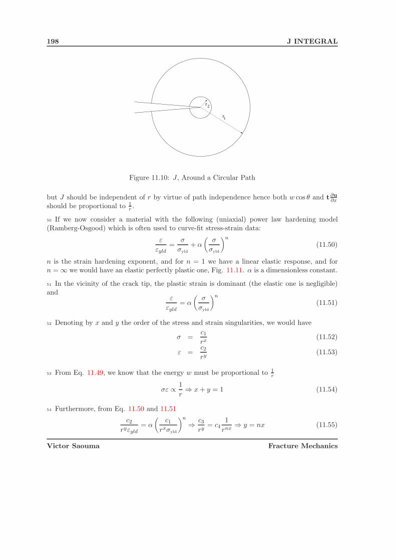
198 J INTEGRAL
r
r2
1
Figure 11.10: J , Around a Circular Path
but J should be independent of r by virtue of path independence hence both w cos θ and t∂u
∂xshould be proportional to 1
r .
50 If we now consider a material with the following (uniaxial) power law hardening model(Ramberg-Osgood) which is often used to curve-fit stress-strain data:
ε
εyld=
σ
σyld
+ α
(σ
σyld
)n
(11.50)
n is the strain hardening exponent, and for n = 1 we have a linear elastic response, and forn = ∞ we would have an elastic perfectly plastic one, Fig. 11.11. α is a dimensionless constant.
51 In the vicinity of the crack tip, the plastic strain is dominant (the elastic one is negligible)and
ε
εyld= α
(σ
σyld
)n
(11.51)
52 Denoting by x and y the order of the stress and strain singularities, we would have
σ =c1
rx(11.52)
ε =c2
ry(11.53)
53 From Eq. 11.49, we know that the energy w must be proportional to 1r
σε ∝ 1
r⇒ x + y = 1 (11.54)
54 Furthermore, from Eq. 11.50 and 11.51
c2
ryεyld= α
(c1
rxσyld
)n
⇒ c3
ry= c4
1
rnx⇒ y = nx (11.55)
Victor Saouma Fracture Mechanics
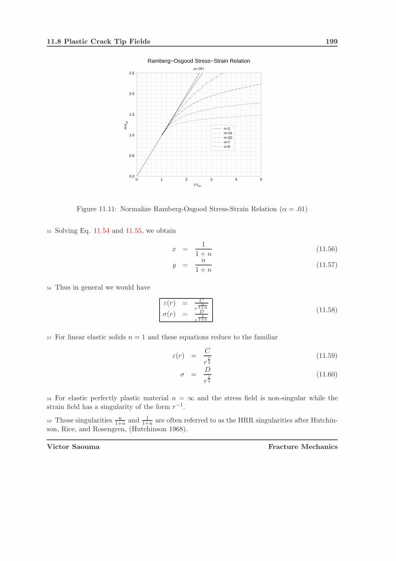
11.8 Plastic Crack Tip Fields 199
0 1 2 3 4 5ε/εyld
0.0
0.5
1.0
1.5
2.0
2.5
σ/σ yl
d
Ramberg−Osgood Stress−Strain Relationα=.001
n=1n=15n=10n=7n=5
Figure 11.11: Normalize Ramberg-Osgood Stress-Strain Relation (α = .01)
55 Solving Eq. 11.54 and 11.55, we obtain
x =1
1 + n(11.56)
y =n
1 + n(11.57)
56 Thus in general we would have
ε(r) = C
rn
1+n
σ(r) = D
r1
1+n
(11.58)
57 For linear elastic solids n = 1 and these equations reduce to the familiar
ε(r) =C
r12
(11.59)
σ =D
r12
(11.60)
58 For elastic perfectly plastic material n = ∞ and the stress field is non-singular while thestrain field has a singularity of the form r−1.
59 Those singularities n1+n and 1
1+n are often referred to as the HRR singularities after Hutchin-son, Rice, and Rosengren, (Hutchinson 1968).
Victor Saouma Fracture Mechanics

200 J INTEGRAL
60 It can be shown that there is a relationship between J and the crack tip σ − ε field:
σij = σyld
(EJ
ασ2yldInr
) 11+n
σij (θ, n) (11.61)
εij =ασyld
E
(EJ
ασ2yldInr
) n1+n
εij(θ, n) (11.62)
where In is an integration constant which depends on the σ−ε curve, and σ & ε are dimensionlessfunctions of n and θ (analogous to f I
ij in LEFM which also depend on the stress state (planestress/strain)
61 Thus, J also characterizes the σ and ε singularities in EPFM just as K did in LEFM (σij =K√2πr
.
62 Finally, we should note that at the crack tip we have two stress singularities, the first one1√r
in the elastic region, and the later 1
r1
1+n
. From Fig. 11.12, we observe that material behind
a propagating crack unload elastically (as opposed to nonlinear elastic). The material directlyin front of the crack also violates our assumption of of proportional loading, i.e. the stresscomponents increase or decrease at different rates. For the crack to be J controlled, those twozones must be embedded within a zone of J dominance. If the crack grows outside it, then themeasured R curve is no longer uniquely characterized by J .
Figure 11.12: HRR Singularity, (Anderson 1995)
63 Fig. 11.13, and table 11.1 schematically illustrate the effect of plasticity on crack tip stresses,where L represents a characteristic dimension of the structure.
Small Scale Yielding: In this zone both K and J characterize this zone. At a short distancefrom the crack tip (relative to L), the stress is proportional to 1√
rand this area is called
the K-dominated region. If we have monotonic loading, a J dominated region occurs inthe plastic zone where the elastic singularity is no longer valid. Inside the plastic zone,the HRR is approximately valid. Finally, finite strain region occurs within approximately2δ from the crack tip where the large deformation invalidates HRR.
Victor Saouma Fracture Mechanics

11.8 Plastic Crack Tip Fields 201
a Large Strain Region b: J-dominated zone; c: Kdominated zone
a
ba
cba
Figure 11.13: Effect of Plasticity on the Crack Tip Stress Fields, (Anderson 1995)
Large Strain J Dominated K Dominated
Small scale yielding Y Y YElastic Plastic Conditions Y Y NLarge Scale Yileding Y N N
Table 11.1: Effect of Plasticity on the Crack Tip Stress Field, (Anderson 1995)
Victor Saouma Fracture Mechanics
202 J INTEGRAL
Elastic-Plastic: J is still valid, but K no longer.
Large Scale Yielding: here the size of the finite strain zone becomes significant relative to Land there is no longer a region uniquely characterized by J . J becomes size and geometrydependent.
11.9 Engineering Approach to Fracture
64 The solution of a plastic problem involves the determination of the J integral. This usuallyinvolves a finite element analysis.
65 If such a capability is not available, and a first order approximation of J is required, then asimplified engineering approach can be followed, (Kumar et al. 1981).
General Solution: For Ramberg-Osgood material, we can write
J = Je(ae) + JP (a, n) (11.63-a)
δ = δe(ae) + δP (a, n) (11.63-b)
Δc = Δec(ae) + ΔPc(a, n) (11.63-c)
where: J , δ, and Δ are the J integral, the crack tip opening displacement, and pointload displacement respectively, and
ae = a + φry (11.64-a)
ry =1
βπ
n − 1
n + 1
(KI
σy
)2
(11.64-b)
φ =1
1 + (P/Po)2 (11.64-c)
for plane stress β = 2 and for plane strain β = 6.
Jp(a, n), δp(a, n), and Δpc(a, n) are the plastic contributions based on the material hard-ening exponent n.
We note that P is the generalized load per unit thickness, Δ is the load-point displacement,and that δ is the crack opening displacement.
Elastic Solution: The elastic solution can be written as
Je = f1
(a
W
)P 2
E′ =K2
I
E′ (11.65-a)
δe = f2
(a
W
)P
E′ (11.65-b)
Δce = f3
(a
W
)P
E′ (11.65-c)
Victor Saouma Fracture Mechanics

11.9 Engineering Approach to Fracture 203
We note that P is the generalized load per unit thickness, and that δ is the crack openingdisplacement.
Fully Plastic Solution: Considering a fully plastic incompressible cracked body, εe � εp.Consider a nonlinear or fully plastic incompressible body and with εe � εp, furthermore,if the plastic deformation can be described by J2, deformation plasticity theory with powerlaw and isotropic hardening, then the small strain constitutive relation is given by
εij
εyld=
3
2α(
σ
σyld)n−1 Sij
σyld(11.66)
where Sij and σe = 32
√SijSij are the stress deviator and the von-Mises effective stress,
respectively.
For such a material Ilyushin (Il’yushin 1946) has shown that the solution of the boundaryvalue problems based on the above equation, and involving a single load or displacementparameter which is increasing monotonically has two important properties:
1. The field quantities increase in direct proportion to the load or displacement para-meter raised to some power dependent on n. For example if the traction is Ti = PT ′
i
and P is a loading parameter, then
σij = Pσ′ij(xi, n) (11.67-a)
εij = αεy
(P
σy
)n
ε′ij(xi, n) (11.67-b)
ui = αεy
(P
σy
)n
u′i(xi, n) (11.67-c)
where σ′ij(xi, n), ε′ij(xi, n) and u′
i(xi, n) are functions of xi and n and are indepen-dent of P .
2. Since σ and ε increase in the same proportion, fully plastic solution based on defor-mation plasticity is also the exact solution to the same problem posed for incrementalor flow theory.
66 Since the integrand of J involves the product of σ and u gradients, then the fully plasticJ will be proportional to Pn+1 and we can write:
Jp = αεyσybg1(a/W )h1(a/W,n)(P/P0)n+1 (11.68-a)
δp = αεyag2(a/W )h2(a/W,n)(P/P0)n (11.68-b)
Δcp = αεyag3(a/W )h3(a/W,n)(P/P0)n (11.68-c)
δtp = αεybg4(a/W )h4(a/W,n)(P/P0)n+1 (11.68-d)
where P0 coresponds to the limit load based on σy and b is the ligament length (W −a).α is from Eq. 11.51 ε/εyld = α(σ/σyld)
n.
Victor Saouma Fracture Mechanics
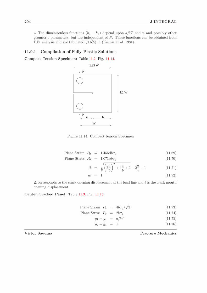
204 J INTEGRAL
67 The dimensionless functions (h1 − h4) depend upon a/W and n and possibly othergeometric parameters, but are independent of P . Those functions can be obtained fromF.E. analysis and are tabulated (±5%) in (Kumar et al. 1981).
11.9.1 Compilation of Fully Plastic Solutions
Compact Tension Specimen: Table 11.2, Fig. 11.14.
1.2 W
1.25 W
P
Pa
W
b
Figure 11.14: Compact tension Specimen
Plane Strain P0 = 1.455βbσy (11.69)
Plane Stress P0 = 1.071βbσy (11.70)
β =
√(2a
b
)2
+ 4a
b+ 2 − 2
a
b− 1 (11.71)
gi = 1 (11.72)
Δ corresponds to the crack opening displacement at the load line and δ is the crack mouthopening displacement.
Center Cracked Panel: Table 11.3, Fig. 11.15
Plane Strain P0 = 4bσy/√
3 (11.73)
Plane Stress P0 = 2bσy (11.74)
g1 = g4 = a/W (11.75)
g2 = g3 = 1 (11.76)
Victor Saouma Fracture Mechanics

11.9 Engineering Approach to Fracture 205
n = 1 n = 2 n = 3 n = 5 n = 7 n = 10 n = 13 n = 16 n = 20
Plane Strain
h1 2.23 2.05 1.78 1.48 1.33 1.26 1.25 1.32 1.57aW
= 14
h2 17.9 12.5 11.7 10.9 10.5 10.7 11.5 12.6 14.6h3 9.85 8.51 8.17 7.77 7.71 7.92 8.52 9.31 10.9
h1 2.15 1.72 1.39 0.97 0.69 0.443 0.28 0.176 0.098aW
= 38
h2 12.60 8.18 6.52 4.32 2.97 1.79 1.10 0.686 0.370h3 7.94 5.76 4.64 3.10 2.14 1.29 0.793 0.494 0.266
h1 1.94 1.51 1.24 0.919 0.68 0.461 0.314 0.216 0.132aW
= 12
h2 9.33 5.85 4.30 2.75 1.91 1.20 0.788 0.530 0.370h3 6.41 4.27 3.16 2.02 1.41 0.998 0.585 0.393 0.236
h1 1.76 1.45 1.24 0.97 0.75 0.602 0.459 0.347 0.248aW
= 58
h2 7.61 4.57 3.42 2.36 1.51 1.32 0.983 0.749 0.485h3 5.52 3.43 2.58 1.79 1.37 1.00 0.746 0.568 0.368
h1 1.71 1.42 1.26 1.03 0.86 0.717 0.575 0.448 0.345aW
= 34
h2 6.37 3.95 3.18 2.34 1.89 1.440 1.120 0.887 0.665h3 4.86 3.05 2.46 1.81 1.45 1.110 0.869 0.686 0.514
h1 1.57 1.45 1.35 1.18 1.08 0.95 0.85 0.73 0.63aW
≈ 1 h2 5.39 3.74 3.09 2.43 2.12 1.80 1.57 1.33 1.14h3 4.31 2.99 2.47 1.95 1.79 1.44 1.26 1.07 0.909
Plane Stress
h1 1.61 1.460 1.28 1.06 0.90 0.729 0.601 0.511 0.395aW
= 14
h2 17.60 12.00 10.70 8.74 7.32 5.74 4.63 3.75 2.92h3 9.67 8.00 7.21 5.94 5.00 3.95 3.19 2.59 2.023
h1 1.55 1.25 1.050 0.801 0.64 0.484 0.377 0.284 0.22aW
= 38
h2 12.40 8.20 6.540 4.56 3.45 2.44 1.83 1.36 1.02h3 7.80 5.73 4.620 3.250 2.48 1.77 1.33 0.99 0.746
h1 1.40 1.08 0.901 0.686 0.55 0.436 0.356 0.298 0.238aW
= 12
h2 9.16 5.67 4.21 2.80 2.12 1.57 1.25 1.03 0.814h3 6.29 4.15 3.11 2.09 1.59 1.18 0.938 0.774 0.614
h1 1.27 1.03 0.875 0.695 0.59 0.494 0.423 0.37 0.310aW
= 58
h2 7.470 4.48 3.35 2.37 1.92 1.540 1.29 1.12 0.928h3 5.42 3.38 2.54 1.80 1.47 1.180 0.988 0.853 0.710
h1 1.23 0.977 0.833 0.683 0.59 0.506 0.431 0.373 0.314aW
= 34
h2 6.25 3.78 2.89 2.14 1.78 1.440 1.20 1.03 0.857h3 4.77 2.92 2.24 1.66 1.38 1.120 0.936 0.80 0.666
h1 1.130 1.01 0.775 0.68 0.65 0.620 0.490 0.47 0.42aW
≈ 1 h2 5.29 3.54 2.41 1.91 1.73 1.59 1.23 1.17 1.03h3 4.23 2.83 1.93 1.52 1.39 1.270 0.985 0.933 0.824
Table 11.2: h-Functions for Standard ASTM Compact Tension Specimen, (Kumar et al. 1981)
Victor Saouma Fracture Mechanics
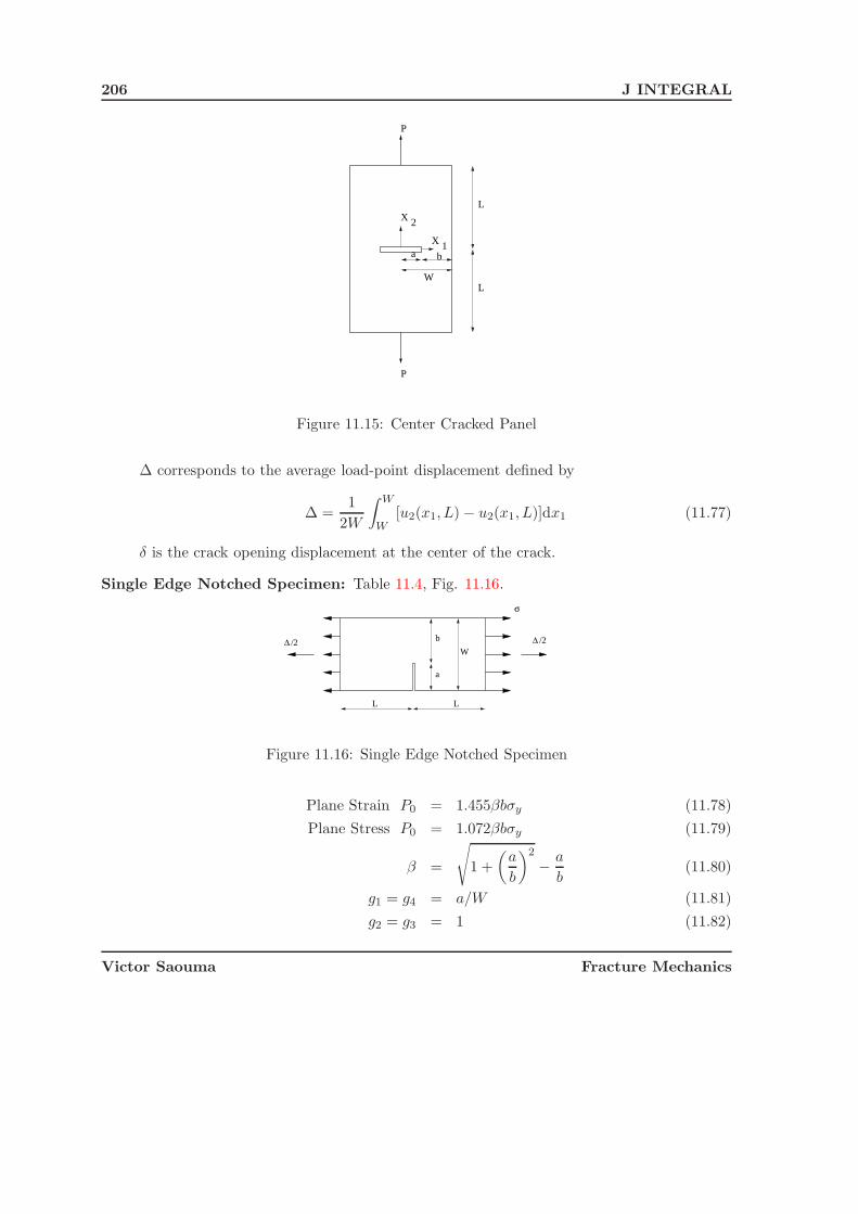
206 J INTEGRAL
P
P
L
LX
Xa b
W
2
1
Figure 11.15: Center Cracked Panel
Δ corresponds to the average load-point displacement defined by
Δ =1
2W
∫ W
W[u2(x1, L) − u2(x1, L)]dx1 (11.77)
δ is the crack opening displacement at the center of the crack.
Single Edge Notched Specimen: Table 11.4, Fig. 11.16.
L L
W
a
b Δ
σ
/2Δ /2
Figure 11.16: Single Edge Notched Specimen
Plane Strain P0 = 1.455βbσy (11.78)
Plane Stress P0 = 1.072βbσy (11.79)
β =
√1 +
(a
b
)2
− a
b(11.80)
g1 = g4 = a/W (11.81)
g2 = g3 = 1 (11.82)
Victor Saouma Fracture Mechanics

11.9 Engineering Approach to Fracture 207
n = 1 n = 2 n = 3 n = 5 n = 7 n = 10 n = 13 n = 16 n = 20
Plane Strain
h1 2.80 3.61 4.06 4.35 4.33 4.02 3.56 3.06 2.46aW
= 18
h2 3.05 3.62 3.91 4.06 3.93 3.54 3.07 2.60 2.06h3 0.303 0.574 0.84 1.30 1.63 1.95 2.03 1.96 1.77
h1 2.54 3.01 3.21 3.29 3.18 2.92 2.63 2.34 2.03aW
= 14
h2 2.68 2.99 3.01 2.85 2.61 2.30 1.00 1.71 1.45h3 0.536 0.911 1.22 1.64 1.84 1.85 1.80 1.64 1.43
h1 2.340 2.62 2.65 2.51 2.28 1.97 1.71 1.46 1.19aW
= 38
h2 2.350 2.39 2.23 1.88 1.58 1.28 1.07 0.89 0.715h3 0.699 1.06 1.28 1.44 1.40 1.23 1.05 0.888 0.719
h1 2.21 2.29 2.20 1.97 1.76 1.52 1.32 1.16 0.978aW
= 12
h2 2.030 1.860 1.60 1.23 1.00 0.799 0.664 0.564 0.466h3 0.803 1.07 1.16 1.10 0.96 0.796 0.665 0.565 0.469
h1 2.12 1.96 1.76 1.43 1.17 0.863 0.628 0.458 0.300aW
= 58
h2 1.71 1.320 1.04 0.707 0.52 0.358 0.250 0.178 0.114h3 0.844 0.937 0.879 0.701 0.52 0.361 0.251 0.178 0.115
h1 2.070 1.73 1.47 1.11 0.89 0.642 0.461 0.337 0.216aW
= 34
h2 1.350 0.857 0.596 0.361 0.25 0.167 0.114 0.081 0.0511h3 805 0.70 0.555 0.359 0.25 0.168 0.114 0.081 0.052
h1 2.08 1.64 1.40 1.14 0.98 0.814 0.688 0.573 0.461aW
= 78
h2 0.889 0.428 0.287 0.181 0.13 0.105 0.084 0.068 0.0533h3 0.632 0.400 0.291 0.182 0.14 0.106 0.084 0.068 0.054
Plane Stress
h1 2.80 3.57 4.01 4.47 4.65 4.62 4.41 4.13 3.72aW
= 18
h2 3.530 4.09 4.43 4.74 4.79 4.63 4.33 4.00 3.55h3 0.350 0.661 1.00 1.55 2.05 2.56 2.83 2.95 2.92
h1 2.54 2.97 3.14 3.20 3.11 2.86 2.65 2.47 2.20aW
= 14
h2 3.100 3.29 3.30 3.15 2.93 2.56 2.29 2.08 1.81h3 0.619 1.01 1.35 1.83 2.08 2.19 2.12 2.01 1.79
h1 2.340 2.53 2.52 2.35 2.17 1.95 1.77 1.61 1.43aW
= 38
h2 2.710 2.62 2.41 2.03 1.75 1.47 1.28 1.13 0.988h3 0.807 1.20 1.43 1.59 1.57 1.43 1.27 1.13 0.994
h1 2.210 2.20 2.06 1.81 1.63 1.43 1.30 1.17 1.00aW
= 12
h2 2.340 2.01 1.70 1.30 1.07 0.871 0.757 0.666 0.557h3 0.927 1.19 1.26 1.18 1.04 0.867 0.758 0.668 0.560
h1 2.12 1.91 1.69 1.41 1.22 1.01 0.853 0.712 0.573aW
= 58
h2 1.970 1.46 1.13 0.785 0.61 0.474 0.383 0.313 0.256h3 0.975 1.05 0.97 0.763 0.62 0.478 0.386 0.318 0.273
h1 2.07 1.71 1.46 1.21 1.08 0.867 0.745 0.646 0.532aW
= 34
h2 1.550 0.97 0.685 0.452 0.36 0.262 0.216 0.183 0.148h3 0.929 0.802 0.642 0.45 0.36 0.263 0.216 0.183 0.149
h1 2.08 1.57 1.31 1.08 0.97 0.862 0.778 0.715 0.630aW
= 78
h2 1.030 0.485 0.31 0.196 0.15 0.127 0.109 0.0971 0.0842h3 0.730 0.452 0.313 0.198 0.15 0.127 0.109 0.0973 0.0842
Table 11.3: Plane Stress h-Functions for a Center-Cracked Panel, (Kumar et al. 1981)
Victor Saouma Fracture Mechanics

208 J INTEGRAL
Δ is the load-point displacement at the centerline of the specimen, and δ is the crackmouth opening displacement.
Double Edge Notched Specimen: Table 11.5, Fig. 11.17.
P,
x
x
L
L
W
b a
Δ/2
P, Δ/2
2
1
Figure 11.17: Double Edge Notched Specimen
Plane Strain P0 = (0.72W + 1.82b)σy (11.83)
Plane Stress P0 = 4bσy/√
3 (11.84)
β =
√1 +
(a
b
)2
− a
b(11.85)
g1 = g4 = 1 (11.86)
g2 = g3 = W/a − 1 (11.87)
Δ is the load-point displacement at the centerline of the specimen, and δ is the crackmouth opening displacement.
Axially Cracked Pressurized Cylinder: Table ??, Fig. 11.18.
p0 =2bσy√3Rc
(11.88)
Rc = Ri + a (11.89)
g1 =a
W(11.90)
g2 = 1 (11.91)
δ is the crack mouth opening displacement. Note that in the elastic range:
KI =2pR2
0
√πa
R20 − R2
i
F
(a
W,Ri
R0
)(11.92)
Victor Saouma Fracture Mechanics

11.9 Engineering Approach to Fracture 209
n = 1 n = 2 n = 3 n = 5 n = 7 n= 10 n = 13 n = 16 n = 20
Plane Strain
h1 4.95 6.93 8.57 11.50 13.5 16.1 18.1 19.9 21.2aW
= 18
h2 5.250 6.47 7.56 9.46 11.1 12.9 14.4 15.7 16.8h3 26.60 25.80 25.20 24.20 23.6 23.2 23.2 23.5 23.7
h1 4.34 4.77 4.64 3.82 3.06 2.170 1.55 1.11 0.712aW
= 14
h2 4.760 4.56 4.28 3.39 2.64 1.910 1.25 0.875 0.552h3 10.30 7.64 5.87 3.70 2.48 1.500 0.97 0.654 0.404
h1 3.88 3.25 2.63 1.68 1.06 0.539 0.276 0.142 0.060aW
= 38
h2 4.540 3.49 2.67 1.57 0.94 0.458 0.229 0.116 0.048h3 5.14 2.99 1.90 0.923 0.51 0.240 0.119 0.060 0.025
h1 3.40 2.30 1.69 0.928 0.51 0.213 0.090 0.039 0.012aW
= 12
h2 4.450 2.77 1.89 0.954 0.50 0.204 0.085 0.036 0.011h3 3.15 1.54 0.91 0.417 0.21 0.085 0.036 0.015 0.004
h1 2.86 1.80 1.30 0.697 0.37 0.153 0.064 0.026 0.008aW
= 58
h2 4.370 2.44 1.62 0.081 0.42 0.167 0.067 0.027 0.008h3 2.31 1.08 0.68 0.329 0.17 0.067 0.027 0.011 0.003
h1 2.34 1.61 1.25 0.769 0.47 0.233 0.116 0.059 0.022aW
= 34
h2 4.320 2.52 1.79 1.03 0.69 0.296 0.146 0.074 0.027h3 2.02 1.10 0.765 0.435 0.26 0.125 0.062 0.031 0.011
h1 1.91 1.57 1.37 1.10 0.92 0.702aW
= 78
h2 4.29 2.75 2.14 1.55 1.23 0.921h3 2.01 1.27 0.988 0.713 0.56 0.424
Plane Stress
h1 3.58 4.55 5.06 5.30 4.96 4.14 3.29 2.60 1.92aW
= 18
h2 5.15 5.43 6.05 6.01 5.47 4.46 3.48 2.74 2.02h3 26.10 21.60 18.00 12.70 9.24 5.98 3.94 2.72 2.00
h1 3.14 3.26 2.920 2.120 1.53 0.96 0.615 0.40 0.23aW
= 14
h2 4.67 4.30 3.700 2.530 1.76 1.05 0.656 0.419 0.237h3 10.10 6.49 4.360 2.190 1.24 0.63 0.362 0.224 0.123
h1 2.81 2.37 1.940 1.370 1.01 0.677 0.474 0.342 0.226aW
= 38
h2 4.47 3.43 2.630 1.690 1.18 0.762 0.524 0.372 0.244h3 5.05 2.65 1.600 0.812 0.525 0.328 0.223 0.157 0.102
h1 2.46 1.67 1.250 0.776 0.510 0.286 0.164 0.0956 0.0469aW
= 12
h2 4.37 2.73 1.91 1.09 0.694 0.380 0.216 0.124 0.0607h3 3.10 1.43 0.871 0.461 0.286 0.155 0.088 0.0506 0.0247
h1 2.07 1.41 1.105 0.755 0.551 0.363 0.248 0.172 0.107aW
= 58
h2 4.30 2.55 1.840 1.160 0.816 0.523 0.353 0.242 0.150h3 2.27 1.13 0.771 0.478 0.336 0.215 0.146 0.100 0.062
h1 1.70 1.14 0.910 0.624 0.447 0.280 0.181 0.118 0.067aW
= 34
h2 4.24 2.47 1.81 1.150 0.798 0.490 0.314 0.203 0.115h3 1.98 1.09 0.784 0.494 0.344 0.211 0.136 0.0581 0.0496
h1 1.38 1.11 0.962 0.792 0.677 0.574aW
= 78
h2 4.22 2.68 2.08 1.54 1.27 1.04h3 1.97 1.25 0.969 0.716 0.592 0.483
Table 11.4: h-Functions for Single Edge Notched Specimen, (Kumar et al. 1981)
Victor Saouma Fracture Mechanics

210 J INTEGRAL
n = 1 n = 2 n = 3 n = 5 n = 7 n = 10 n = 13 n = 16 n = 20
Plane Strain
h1 0.572 0.772 0.922 1.13 1.35 1.61 1.86 2.09 2.44aW
= 18
h2 0.732 0.852 0.961 1.14 1.29 1.50 1.70 1.94 2.17h3 0.063 0.126 0.200 0.372 0.57 0.911 1.30 1.74 2.29
h1 1.10 1.320 1.38 1.65 1.75 1.82 1.86 1.89 1.92aW
= 14
h2 1.56 1.63 1.70 1.79 1.80 1.81 1.79 1.78 1.76h3 0.267 0.479 0.698 1.11 1.47 1.92 2.25 2.49 2.73
h1 1.61 1.83 1.92 1.92 1.84 1.68 1.49 1.32 1.12aW
= 38
h2 2.51 2.41 2.35 2.15 1.94 1.68 1.44 1.25 1.05h3 0.637 1.05 1.40 1.87 2.11 2.20 2.09 1.92 1.67
h1 2.22 2.43 2.49 2.43 2.32 2.12 1.91 1.60 1.51aW
= 12
h2 3.73 3.40 3.15 2.70 2.37 2.01 1.72 1.40 1.38h3 1.26 1.92 2.37 2.79 2.85 2.68 2.40 1.99 1.94
h1 3.16 3.38 3.45 3.42 3.28 3.00 2.54 2.36 2.27aW
= 58
h2 5.57 4.76 4.23 3.46 2.97 2.48 2.02 1.82 1.66h3 2.36 3.29 3.74 3.90 3.68 3.23 2.66 2.40 2.19
h1 5.24 6.29 7.17 8.44 9.46 10.90 119.0 11.3 17.4aW
= 34
h2 9.10 7.76 7.14 6.64 6.83 7.48 7.790 7.14 11.0h3 4.73 6.26 7.03 7.63 8.14 9.04 9.4 8.58 13.5
h1 14.2 24.8 39.0 78.4 140. 341.0 777.0 1570.0 3820.0aW
= 78
h2 20.1 19.4 22.7 36.1 58.9 133.0 294.0 585.0 1400.0h3 12.7 18.2 24.1 40.4 65.9 149.0 327.0 650.0 1560.0
Plane Stress
h1 0.583 0.825 1.02 1.37 1.71 2.24 2.84 3.54 4.62aW
= 18
h2 0.853 1.050 1.23 1.55 1.87 2.38 2.96 3.65 4.70h3 0.0729 0.159 0.26 0.504 0.82 1.41 2.18 3.16 4.73
h1 1.01 1.23 1.36 1.48 1.54 1.58 1.59 1.59 1.59aW
= 14
h2 1.73 1.82 1.89 1.92 1.91 1.85 1.80 1.75 1.70h3 0.296 0.537 0.77 1.17 1.49 1.82 2.02 2.12 2.20
h1 1.29 1.42 1.43 1.34 1.24 1.09 0.97 0.873 0.674aW
= 38
h2 2.59 2.39 2.22 1.86 1.59 1.28 1.07 0.922 0.709h3 658 1.04 1.30 1.52 1.55 1.41 1.23 1.07 0.830
h1 1.48 1.47 1.38 1.17 1.01 0.845 0.732 0.625 0.208aW
= 12
h2 3.51 2.82 2.34 1.67 1.28 0.944 0.762 0.630 0.232h3 1.18 1.58 1.69 1.56 1.32 1.01 0.809 0.662 0.266
h1 1.59 1.45 1.29 1.04 0.88 0.737 0.649 0.466 0.020aW
= 58
h2 4.56 3.15 2.32 1.45 1.06 0.790 0.657 0.473 0.028h3 1.93 2.14 1.95 1.44 1.09 0.809 0.665 0.487 0.032
h1 1.65 1.43 1.22 0.979 0.83 0.701 0.630 0.297aW
= 34
h2 5.90 3.37 2.22 1.30 0.96 0.741 0.636 0.312h3 3.06 2.67 2.06 1.31 0.97 0.747 0.638 0.318
h1 1.69 1.43 1.22 0.979 0.84 0.738 0.664 0.614 0.562aW
= 78
h2 8.02 3.51 2.14 1.27 0.97 0.775 0.663 0.596 0.535h3 5.07 3.180 2.16 1.30 0.98 0.779 0.665 0.597 0.538
Table 11.5: h-Functions for Double Edge Notched Specimen, (Kumar et al. 1981)
Victor Saouma Fracture Mechanics

11.9 Engineering Approach to Fracture 211
R
R
o
i
p
p
a b
W
Figure 11.18: Axially Cracked Pressurized Cylinder
δe =8pR2
0a
(R20 − R2
i )E′V(
a
W,Ri
R0
)(11.93)
where the dimensionless functions F and V are tabulated in Table 11.7.
Circumferentially Cracked Cylinder: Table 11.8, Fig. 11.19.
P0 =2πσy(R
20 − R2
i )√3
(11.94)
Rc = Ri + a (11.95)
g1 = g4 =a
W(11.96)
g2 = g3 = 1 (11.97)
δ is the crack mouth opening displacement.
In the elastic range
KI = σ√
πaF
(a
W,Ri
R0
)(11.98)
δe =4σaV1
(aW , Ri
R0
)E′ (11.99)
Δce =4σaV2
(aW , Ri
R0
)E′ (11.100)
where the functions F , V1, and V2 are tabulated in Table 11.9.
Victor Saouma Fracture Mechanics

212 J INTEGRAL
n = 1 n = 2 n = 3 n = 5 n = 7 n = 10WRi
= 15
aW
= 18
h1 6.32 7.93 9.32 11.50 13.1 14.94h2 5.83 7.01 7.96 9.49 10.6 11.96
aW
= 14
h1 7.00 9.34 9.03 9.59 9.71 9.45h2 5.92 8.72 7.07 7.26 7.14 6.71
aW
= 12
h1 9.79 10.37 9.07 5.61 3.52 2.11h2 7.05 6.97 6.01 3.70 2.28 1.25
aW
= 34
h1 11.00 5.54 2.84 1.24 0.83 0.493h2 7.35 3.86 1.86 0.56 0.26 0.129
WRi
= 110
aW
= 18
h1 5.22 6.64 7.59 8.76 9.34 9.55h2 5.31 6.25 6.88 7.65 8.02 8.09
aW
= 14
h1 6.16 7.49 7.96 8.08 7.78 6.98h2 5.56 6.31 6.52 6.40 6.01 5.27
aW
= 12
h1 10.5 11.6 10.7 6.47 3.95 2.27h2 7.48 7.72 7.01 4.29 2.58 1.37
aW
= 34
h1 16.10 8.19 3.87 1.46 1.05 0.787h2 9.57 5.40 2.57 0.71 0.37 0.232
WRi
= 120
aW
= 18
h1 4.50 5.79 6.62 7.65 8.07 7.75h2 4.96 5.71 6.20 6.82 7.02 6.66
aW
= 14
h1 5.57 6.91 7.37 7.47 7.21 6.53h2 5.29 5.98 6.16 6.01 5.63 4.93
aW
= 12
h1 10.80 12.80 12.80 8.16 4.88 2.62h2 7.66 8.33 8.13 5.33 3.20 1.65
aW
= 34
h1 23.10 13.10 5.87 1.90 1.23 0.883h2 12.10 7.88 3.84 1.01 0.45 0.24
Table 11.6: h-Functions for an Internally Pressurized, Axially Cracked Cylinder, (Kumar et al.1981)
aW
= 18
aW
= 14
aW
= 12
aW
= 34
WRI
= 15
F 1.19 1.38 2.10 3.30
V1 1.51 1.83 3.44 7.50WRI
= 110
F 1.20 1.44 2.36 4.23
V1 1.54 1.91 3.96 10.40WRI
= 120
F 1.20 1.45 2.51 5.25
V1 1.54 1.92 4.23 13.50
Table 11.7: F and V1 for Internally Pressurized, Axially Cracked Cylinder, (Kumar et al. 1981)
Victor Saouma Fracture Mechanics
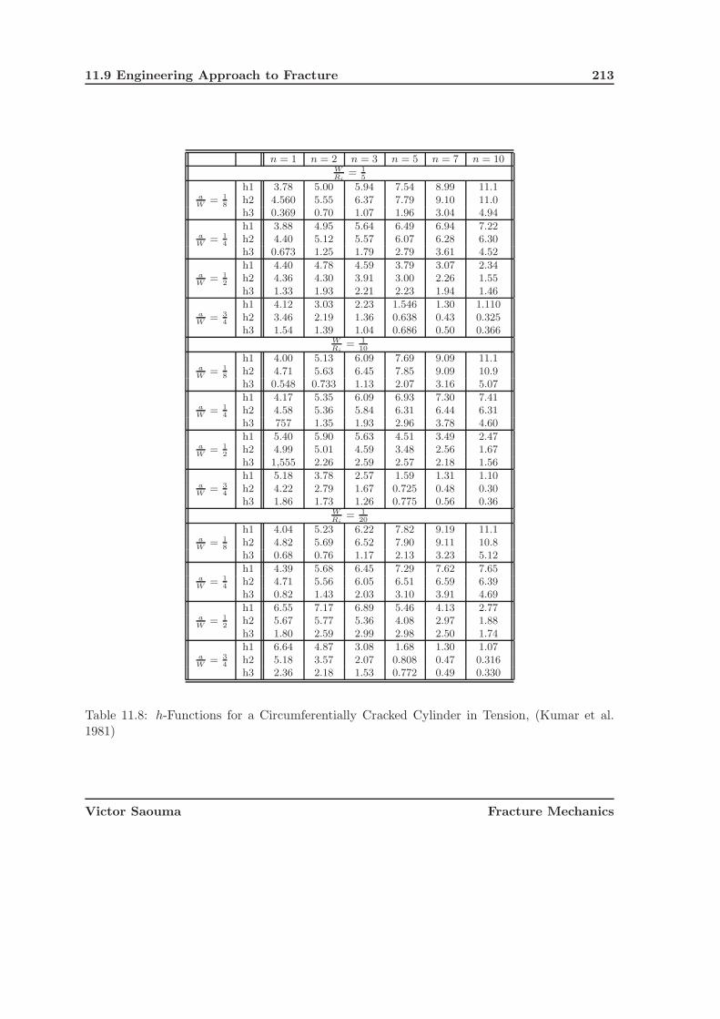
11.9 Engineering Approach to Fracture 213
n = 1 n = 2 n = 3 n = 5 n = 7 n = 10WRi
= 15
h1 3.78 5.00 5.94 7.54 8.99 11.1aW
= 18
h2 4.560 5.55 6.37 7.79 9.10 11.0h3 0.369 0.70 1.07 1.96 3.04 4.94
h1 3.88 4.95 5.64 6.49 6.94 7.22aW
= 14
h2 4.40 5.12 5.57 6.07 6.28 6.30h3 0.673 1.25 1.79 2.79 3.61 4.52
h1 4.40 4.78 4.59 3.79 3.07 2.34aW
= 12
h2 4.36 4.30 3.91 3.00 2.26 1.55h3 1.33 1.93 2.21 2.23 1.94 1.46
h1 4.12 3.03 2.23 1.546 1.30 1.110aW
= 34
h2 3.46 2.19 1.36 0.638 0.43 0.325h3 1.54 1.39 1.04 0.686 0.50 0.366
WRi
= 110
h1 4.00 5.13 6.09 7.69 9.09 11.1aW
= 18
h2 4.71 5.63 6.45 7.85 9.09 10.9h3 0.548 0.733 1.13 2.07 3.16 5.07
h1 4.17 5.35 6.09 6.93 7.30 7.41aW
= 14
h2 4.58 5.36 5.84 6.31 6.44 6.31h3 757 1.35 1.93 2.96 3.78 4.60
h1 5.40 5.90 5.63 4.51 3.49 2.47aW
= 12
h2 4.99 5.01 4.59 3.48 2.56 1.67h3 1,555 2.26 2.59 2.57 2.18 1.56
h1 5.18 3.78 2.57 1.59 1.31 1.10aW
= 34
h2 4.22 2.79 1.67 0.725 0.48 0.30h3 1.86 1.73 1.26 0.775 0.56 0.36
WRi
= 120
h1 4.04 5.23 6.22 7.82 9.19 11.1aW
= 18
h2 4.82 5.69 6.52 7.90 9.11 10.8h3 0.68 0.76 1.17 2.13 3.23 5.12
h1 4.39 5.68 6.45 7.29 7.62 7.65aW
= 14
h2 4.71 5.56 6.05 6.51 6.59 6.39h3 0.82 1.43 2.03 3.10 3.91 4.69
h1 6.55 7.17 6.89 5.46 4.13 2.77aW
= 12
h2 5.67 5.77 5.36 4.08 2.97 1.88h3 1.80 2.59 2.99 2.98 2.50 1.74
h1 6.64 4.87 3.08 1.68 1.30 1.07aW
= 34
h2 5.18 3.57 2.07 0.808 0.47 0.316h3 2.36 2.18 1.53 0.772 0.49 0.330
Table 11.8: h-Functions for a Circumferentially Cracked Cylinder in Tension, (Kumar et al.1981)
Victor Saouma Fracture Mechanics

214 J INTEGRAL
R
R
a b
i
o
σσ
σ σ
W
Figure 11.19: Circumferentially Cracked Cylinder
aW
= 18
aW
= 14
aW
= 12
aW
= 34
F 1.16 1.26 1.61 2.15WRI
= 15
V1 1.49 1.67 2.43 3.76
V2 0.117 0.255 0.743 1.67
F 1.19 1.32 1.82 2.49WRI
= 110
V1 1.55 1.76 2.84 4.72
V2 0.18 0.29 0.885 2.09
F 1.22 1.36 2.03 2.89WRI
= 120
V1 1.59 1.81 3.26 5.99
V2 0.22 0.32 1.04 2.74
Table 11.9: F , V1, and V2 for a Circumferentially Cracked Cylinder in Tension, (Kumar et al.1981)
Victor Saouma Fracture Mechanics
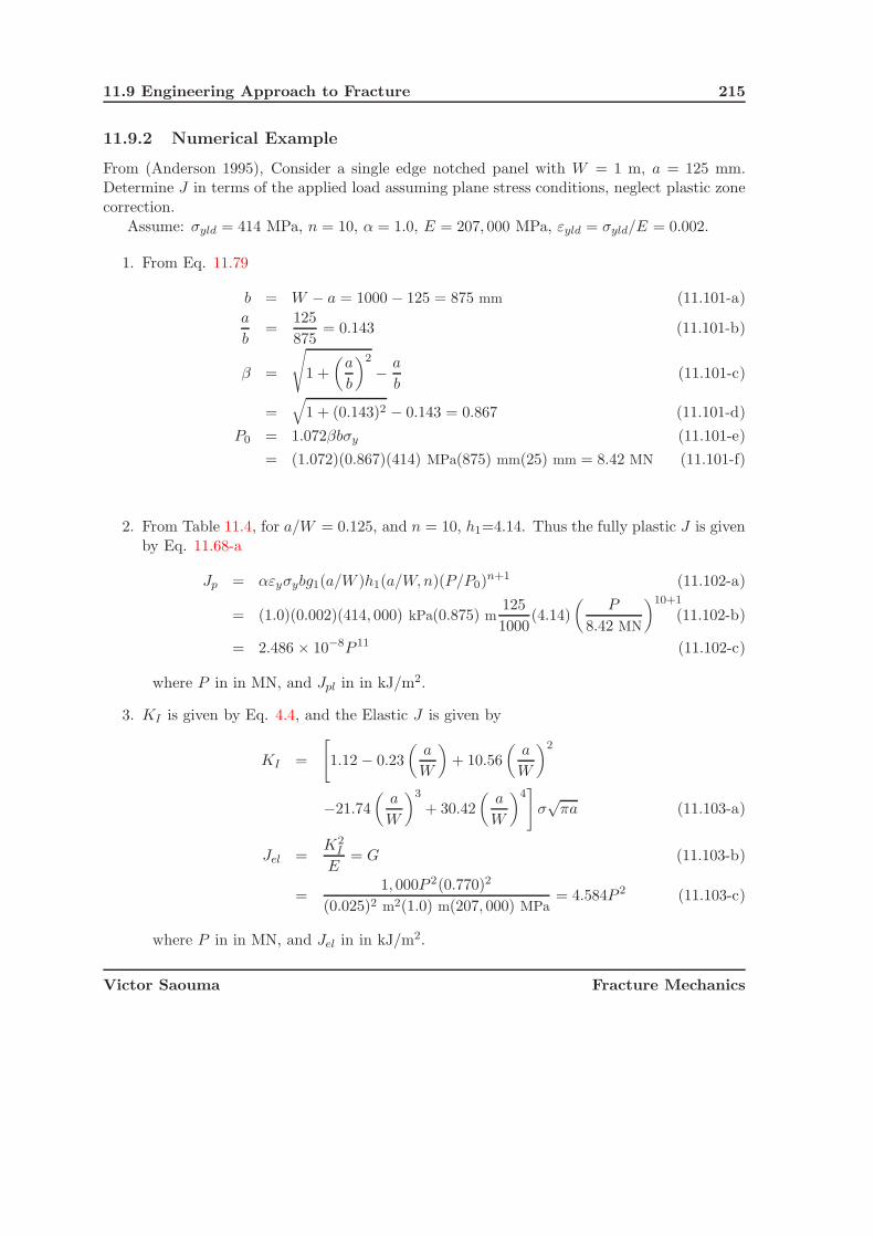
11.9 Engineering Approach to Fracture 215
11.9.2 Numerical Example
From (Anderson 1995), Consider a single edge notched panel with W = 1 m, a = 125 mm.Determine J in terms of the applied load assuming plane stress conditions, neglect plastic zonecorrection.
Assume: σyld = 414 MPa, n = 10, α = 1.0, E = 207, 000 MPa, εyld = σyld/E = 0.002.
1. From Eq. 11.79
b = W − a = 1000 − 125 = 875 mm (11.101-a)
a
b=
125
875= 0.143 (11.101-b)
β =
√1 +
(a
b
)2
− a
b(11.101-c)
=√
1 + (0.143)2 − 0.143 = 0.867 (11.101-d)
P0 = 1.072βbσy (11.101-e)
= (1.072)(0.867)(414) MPa(875) mm(25) mm = 8.42 MN (11.101-f)
2. From Table 11.4, for a/W = 0.125, and n = 10, h1=4.14. Thus the fully plastic J is givenby Eq. 11.68-a
Jp = αεyσybg1(a/W )h1(a/W,n)(P/P0)n+1 (11.102-a)
= (1.0)(0.002)(414, 000) kPa(0.875) m125
1000(4.14)
(P
8.42 MN
)10+1
(11.102-b)
= 2.486 × 10⁻⁸P 11 (11.102-c)
where P in in MN, and Jpl in in kJ/m2.
3. KI is given by Eq. 4.4, and the Elastic J is given by
KI =
[1.12 − 0.23
(a
W
)+ 10.56
(a
W
)2
−21.74
(a
W
)3
+ 30.42
(a
W
)4]
σ√
πa (11.103-a)
Jel =K2
I
E= G (11.103-b)
=1, 000P 2(0.770)2
(0.025)2 m2(1.0) m(207, 000) MPa= 4.584P 2 (11.103-c)
where P in in MN, and Jel in in kJ/m2.
Victor Saouma Fracture Mechanics

216 J INTEGRAL
4. The total J is
J = Jel + Jpl (11.104-a)
= 4.584P 2 + 2.486 × 10⁻⁸P 11 (11.104-b)
0 1 2 3 4 5 6 7 8 9Applied Load [MN]
0
100
200
300
400
500
600
700
800
900
1000
J In
tegr
al [k
J/m
2 ]
JElastic
JPlastic
J
11.10 J1 and J2 Generalization.
66 Rice has shown that in linear elastic fracture, and in terms of the stress intensity factors, Jcan be written as:
(1 − ν2)(K2I + K2
II) + (1 + ν)K2III = EJ1 (11.105)
where J1 is expressed in indicial notation by:
J1 =
∫Γ
(wdy − t
∂u
∂xdΓ
)(11.106)
=
∫Γ
(wn1 − ti
∂ui
∂x1dΓ
)(11.107)
where w is the strain energy density, ni are the direction cosines of the normal to the contour,the Ti are the components of traction, and the contour of integration is around the tip.
67 Knowles and Stenberg (1972) noted that this can be considered as the first component of avector
Jk =
∫{wnk − ti
∂ui
∂xk}dΓ (11.108)
which is also path independent. When written in vector form, this gives
J1 =∫Γ
(wdy − t∂u
∂xdΓ)
J2 =∫Γ
(wdx − t∂u
∂y dΓ) (11.109)
Victor Saouma Fracture Mechanics

11.11 Dynamic Energy Release Rate 217
68 Hellen and Blackburn (1975a) showed that
J = J1 − iJ2 (11.110)
=(1 + ν)(1 + κ)
4E(K2
I + K2II + 2iKIKII) (11.111)
69 Thus the values of energy release rates (J1 and J2) for crack extensions parallel and perpen-dicular to the crack, respectively, will be given by:
J1 =K2
I+K2
II
H
J2 = −2KIKII
H
(11.112)
where
H =
{E plane strain
E1−ν2 plane stress
(11.113)
Note that solution of Eq. 11.112 and 11.112 is the intersection of a circle and a hyperbola.Hence, there exists more than one pair of stress intensity factors (or none).
11.11 Dynamic Energy Release Rate
70 If we consider a body containing a propagating crack, (Kanninen 1984), Fig. 11.20
1
a(t)
Ω
X
V
0Γ
2
Γ
X
Figure 11.20: Dynamic Crack Propagation in a Plane Body, (Kanninen 1984)
71 We seek to determine the energy released to the crack tip and thus consider a vanishinglysmall loop Γ0 surrounding the crack tip1. Whereas the loop can have any shape, it must remainfixed relative to a coordinate system attached to the crack tip. We consider the area A boundedby the outer boundary Γ, the traction free crack faces, and the inner loop Γ0.
1in contrast to the static case, the energy release rate can not be expressed by a path-independent contourintegral because if a wave front intercepts one contour, but not the second one, then two different values wouldbe represented by only the contour integral.
Victor Saouma Fracture Mechanics

218 J INTEGRAL
72 The rate of work P done by the tractions on Γ is equal to the rate of increase of the strainenergy U and kinetic energy T in region A and the flux F of energy into the crack tip region:
P = U + T + F (11.114)
where
P =
∫Γ
tiuidΓ (11.115-a)
U = limΓ0→0
∫A
W (εij)dA (11.115-b)
T = limΓ0→0
∫A
1
2ρuiuidA (11.115-c)
73 Since the loop Γ0 moves with the crack tip, region A is time dependent. Therefore, the timerate of change of the strain energy equals the integral over A of the time rate of change of thestrain energy density W (εij) less the flow of this density through the loop Γ0. Hence,
U = limΓ0→0
∫A
W (εij)dA − limΓ0→0
∫Γ0
W (εij)VndΓ (11.116)
where Vn = V n1 = V cos θ is the component of the crack-tip velocity normal to Γ0 and θ is theangle that the outward unit normal to Γ0 makes with the x1 direction.
74 Thus,
dw = σijdεij (11.117-a)
W = σij εij = σij ui,j (11.117-b)
U = limΓ0→0
∫A
σijui,jdA − limΓ0→0
∫Γ0
W (εij)VndΓ (11.117-c)
T = limΓ0→0
∫A
ρuiuidA − limΓ0→0
∫Γ0
1
2ρuiuiVndΓ (11.117-d)
75 Substituting into Eq. 11.114 we obtain
F = limΓ0→0
∫Γ0
(W +
1
2ρuiui
)VndΓ +
∫Γ
tiuidΓ − limΓ0→0
∫A(σij ui,j + ρuiui)dA (11.118)
76 We then useσij ui,j = (σij ui),j − σij,jui (11.119)
and the equation of motionσij,j = ρui (11.120)
Victor Saouma Fracture Mechanics

11.12 Effect of Other Loading 219
and the divergence theorem, then Eq. 11.118 reduces to
F = limΓ0→0
∫Γ0
[(W +
1
2ρuiui
)Vn + tiui
]dΓ (11.121)
77 This is the rate at which energy is lost from the body due to flux through Γ0. This lastequation can be rewritten in terms of the strain energy density w, and the kinetic energydensity t (not to be confused with the traction),
F = limΓ0→0
∫Γ0
[(w + t)V δ1j + σjiui]njdΓ (11.122)
78 In an increment of time dt, the crack extends by da = V dt and the energy expended is Fdt.Thus the energy release rate is
J =F
V(11.123)
79 If we have a moving coordinate system x − y attached to the crack tip where x = X − a(t)and y = Y , then
ui = −V∂ui
∂x+
∂ui
∂t(11.124)
under steady condition, the second term is equal to zero. On the other hand, close to thecrack tip the displacement changes rapidly with position (at a fixed time) and the first termdominates in all cases, ?? thus
J = limΓ0→0
∫Γ0
[(w + t)δ1j − σji
∂ui
∂x
]njdΓ (11.125)
or
J = limΓ0→0
∫Γ0
[(w + t)dy − σjinj
∂ui
∂xdΓ
](11.126)
This equation applies to all types of material.
11.12 Effect of Other Loading
This section is taken from (Reich 1993)
11.12.1 Surface Tractions on Crack Surfaces
80 J integral was first extended by (Karlsson and Backlund 1978) to account for the effect ofsurface tractions on the crack surfaces involves simply extending the definition of the contourpath to include the crack surfaces. The resulting form of the J integral was then given as
J =
∫Γ(W dx2 − tj uj,1 dΓ) −
∫Γt
tj uj,1 dΓ (11.127)
Victor Saouma Fracture Mechanics

220 J INTEGRAL
where Γt is that portion of the upper and lower crack surfaces between the points where Γ endsand begins and ti is the applied surface traction vector.
81 The strain energy density W is absent from the integral over Γt since the crack surfacesare coincident with the negative x1-axis and there is no need to integrate in the x2-direction.Unfortunately, (Karlsson and Backlund 1978) offered no proof showing that path independencewas maintained and a significant portion of their discussion was devoted to the finite elementimplementation of this procedure.
82 Proof of path independence for this procedure was later provided by (Atluri 1982) using thecontour paths shown in Figure 21.1. The proof was given for the Ji integral, therefore, thestrain energy density W is retained in the integrand of the integral accounting for the appliedsurface tractions ti
Ji =
∫Γ(W ni − tj uj,i) dΓ +
∫Γt
(W ni − tj uj,i) dΓ (11.128)
where Γt = Γ+t ∪ Γ−
t .
11.12.2 Body Forces
83 The most straightforward method to account for body forces in the J integral is to addcorrection terms in the form of volume integrals such that path independence is maintained.When body forces are present σij,j = −bi and W,i �= (σjkuj,i),k. Therefore, the integrand ofvolume form of the standard Ji integral (i.e. Equation ??) does not vanish, but instead is
Ji =
∫Ω(bj uj,i) dΩ �= 0 (11.129)
where bj is the body force vector. This means that the strain energy density W is a functionof position and that (W,i)exp �= 0, where (W,i)exp is the gradient of that portion of W thatdepends explicitly on xi.
84 For path independence to be maintained in the presence of body forces the volume integralshown above must be subtracted from the standard line integral form of the Ji integral
Ji =
∫Γ(W ni − tj uj,i) dΓ −
∫Ω(bj uj,i) dΩ (11.130)
which corresponds to the form proposed by (Atluri 1982).
11.12.3 Initial Strains Corresponding to Thermal Loading
85 In order to apply the Ji integral to problems in thermo-elasticity the strain energy density Wmust first be redefined. Looking forward to the presentation of the extension in which thermal
Victor Saouma Fracture Mechanics

11.12 Effect of Other Loading 221
strains and pore pressures will be considered in combination, W will be defined in terms of thenet strains εij and the net effective stresses σ′
ij as
W =
∫ εij
0σ′
ij dεij (11.131)
and the net effective stresses σ′ij being defined as
σ′ij =
∂W
∂εij(11.132)
86 It must be noted that in the absence of initial stresses σ0ij that σij = σ′
ij , where σij are thetotal stresses. Therefore, σ′
ij can be replaced by σij throughout this discussion. For a linearelastic material W is defined as
W =1
2Cijkl εij εkl (11.133)
and the resulting constitutive law is
σ′ij = Cijkl εkl = Cijkl (εkl − αT δkl) (11.134)
which is identical to Equation 21.53.
87 Since the definition of the strain energy density W is now in terms of the net effective stressesσ′
ij, the Ji integral must also be defined in terms of σ′ij rather than the total stresses σij. The
appropriate form of the Ji integral is
Ji =
∫Γ(W ni − t′j uj,i) dΓ (11.135)
where t′i = σ′ijnj are the net effective surface tractions. On application of Green’s theorem to
the line integral form of Ji the resulting volume integral form is
Ji =
∫Ω[W,i − (σ′
jk uj,i),k] dΩ (11.136)
88 Some changes are also required in the definition of W,i due to the change in the definition ofW . The chain rule is still applied to obtain
W,i =∂W
∂εjk
∂εjk
∂xi(11.137)
but ∂εjk/∂xi is defined as
∂εjk
∂xi=
∂εjk
∂xi−
∂ε0jk
∂xi(11.138)
reflecting the contributions of the total and thermal strains, εjk and ε0jk, respectively. ∂εjk/∂xi
is defined as∂εjk
∂xi=
1
2[(uj,k),i + (uk,j),i] =
1
2[(uj,i),k + (uk,i),j ] (11.139)
Victor Saouma Fracture Mechanics

222 J INTEGRAL
and ∂ε0jk/∂xi is defined as
∂ε0jk
∂xi= α T,i δjk (11.140)
89 Recalling that σjk = σkj and substituting the above expressions for ∂εjk/∂xi and ∂ε0jk/∂xi
into Equation 11.137 the expression for W,i can be rewritten as
W,i = σ′jk [(uj,i),k − α T,i δjk] (11.141)
and inserted into Equation 11.136, the volume integral form of Ji. The expression for W,i
clearly includes the σ′jk(uj,i),k term that also results from (σ′
jkuj,i),k. Therefore, in the absenceof body forces σ′
jk,k = 0 and W,i �= (σ′jkuj,i),k, leaving only a term involving T,i in the integrand
of the volume form of the Ji integral
Ji = −∫Ω(α σ′
jj T,i) dΩ �= 0 (11.142)
where σ′jj is the trace of the net effective stress tensor.
90 This means that W is function of position due to the presence of the thermal strains ε0jk and
that (W,i)exp �= 0. To maintain path independence the volume integral shown above must besubtracted from the standard line integral form of Ji yielding
Ji =
∫Γ(W ni − t′j uj,i) dΓ +
∫Ω(α σ′
jj T,i) dΩ (11.143)
which corresponds to the form proposed by (Shih, Moran and Nakamura 1986) if the net effectivestresses are replaced by the total stresses.
91 Including body forces along with the thermal strains at this point is actually quite simple.Recalling that σ′
jk,k = −b′j in the presence of body forces the integrand of the volume form ofthe Ji integral will also include a term involving bj
Ji = −∫Ω(α σ′
jj T,i − b′j uj,i) dΩ �= 0 (11.144)
92 To maintain path independence this volume integral must be subtracted from the standardline integral form of Ji to obtain
Ji =
∫Γ(W ni − t′j uj,i) dΓ +
∫Ω(α σ′
jj T,i − b′j uj,i) dΩ (11.145)
which is quite clearly a simple combination of Equations 11.143 and 11.129.
Victor Saouma Fracture Mechanics

11.12 Effect of Other Loading 223
11.12.4 Initial Stresses Corresponding to Pore Pressures
93 As was the case when the Ji integral was applied to problems in thermo-elasticity, the strainenergy density W must also be redefined for problems in poro-elasticity. However, in this casethe redefinition is more cosmetic in nature, with W being defined in terms of the total strainsεij and the effective stresses σ′
ij as
W =
∫ εij
0σ′
ij dεij (11.146)
and the effective stresses σ′ij are defined as
σ′ij =
∂W
∂εij(11.147)
94 It must be noted that this definition of W is identical to the one given in Equation ??, whereσij was used in lieu of σ′
ij . However, since initial strains and stresses were not considered inEquation ??, σij = σ′
ij and this notation was valid, albeit slightly misleading. For a linearelastic material W is defined as
W =1
2Cijkl εij εkl (11.148)
resulting in the following constitutive law
σ′ij = Cijkl εkl (11.149)
95 The stress-strain relationship defining the total stresses σij is obtained by simply addingexpressions for the initial stresses σ0
ij and the effective stresses σ′ij, as is dictated by the principle
of effective stressσij = Cijkl εkl + σ0
ij = Cijkl εkl − p δij (11.150)
which is identical to Equation 21.62.
96 Since the definition of the strain energy density W is now in terms of the effective stressesσ′
ij, the Ji integral must also be defined in terms of σ′ij rather than the total stresses σij. This
would also seem to be in agreement with of the classical interpretation of the effective stresses(Terzaghi and Peck 1967), where σ′
ij are the only stresses acting on the skeleton of the porousmaterial, which is in fact what is being fractured. The appropriate form of the Ji integral is
Ji =
∫Γ(W ni − t′j uj,i) dΓ (11.151)
where t′i = σ′ijnj are the effective surface tractions.
97 This form of the Ji integral is valid so long as the only source of applied surface tractions tion the crack surfaces is from fluid in the crack, since in this case σ′
ij = 0 and t′i = 0, where t′i are
Victor Saouma Fracture Mechanics

224 J INTEGRAL
the applied effective surface tractions. On application of Green’s theorem to the line integralform of Ji the resulting volume integral form is
Ji =
∫Ω[W,i − (σ′
jkuj,i),k] dΩ (11.152)
98 Based on the expression for W given in Equation 11.146 and the previous proofs W,i canimmediately be written as
W,i =∂W
∂εij
∂εij
∂xi= σ′
jk (uj,i),k (11.153)
and inserted in Equation 11.152, the volume integral form of Ji. In the absence of body forcesσ′
jk,k = p,kδjk and W,i �= (σ′jkuj,i),k, leaving only the term involving p,k in the integrand of the
volume form of Ji integral
Ji = −∫Ω
p,k δjk uj,i dΩ = −∫Ω
p,j uj,i dΩ �= 0 (11.154)
where p,j is the gradient of the pore pressures. This means that W is a function of positiondue the presence of the pore pressures and that (W,i)exp = 0.
99 To maintain path independence the volume integral shown above must be subtracted fromthe standard line integral form of Ji yielding
Ji =
∫Γ(W ni − t′j uj,i) dΓ +
∫Ω
p,j uj,i dΩ (11.155)
which is analogous to the form proposed by (Shih et al. 1986) for problems in thermo-elasticity.
100 Including body forces along with the pore pressures, which is typically the case for problemsin poro-elasticity, is actually quite simple at this point. Recalling that σ′
jk,k = −b′j in thepresence of body forces, where the effective body forces b′j are defined in Equation 21.64, theintegrand of the volume form of the Ji integral can be written in one of two ways
Ji = −∫Ω
b′j uj,i dΩ = −∫Ω(bj − p,j)uj,i dΩ �= 0 (11.156)
with the latter form being somewhat more illuminating than the former.
101 To maintain path independence this volume integral must be subtracted from the standardline integral form of Ji to obtain
Ji =
∫Γ(W ni − t′j uj,i) dΓ −
∫Ω(bj − p,j)uj,i dΩ (11.157)
which is quite clearly a simple combination of Equations 11.155 and 11.129.
Victor Saouma Fracture Mechanics

11.12 Effect of Other Loading 225
11.12.5 Combined Thermal Strains and Pore Pressures
102 In the presence of both thermal strains and pore pressures the strain energy density W isdefined in terms of the net strain tensor εij and the net effective stress tensor σ′
ij, just as it wasin Equation 11.131 for problems in thermo-elasticity. The resulting constitutive law, as definedby Equation 11.134, is substituted into the principle of effective stress to obtain a stress-strainrelationship defining the total stresses σij
σij = Cijkl εkl + σ0ij = Cijkl (εkl − α T δkl) − p δij (11.158)
which is identical to Equation 21.66. Of course, this stress-strain relationship is valid only solong as all initial stresses correspond to pore pressures.
103 Since the definition of the strain energy density W corresponds to that given for problemsin thermo-elasticity the form of the Ji integral and the gradient of the strain energy densityW,i will also correspond to those for problems in thermo-elasticity. Therefore, when thermalstrains and pore pressures are considered in combination the line integral form of Ji is given byEquation 11.135; the volume integral form of Ji is given by Equation 11.136; and the expressionfor W,i is given by Equation 11.137.
104 However, in the absence of body forces σ′jk,k = p,kδjk rather than σ′
jk,k = 0, as it was in thesame situation for problems in thermo-elasticity, and W,i �= (σ′
jkuj,i),k, leaving terms involvingboth T,i and p,j in the integrand of the volume form of Ji integral
Ji = −∫Ω(α σ′
jj T,i + p,j uj,i) dΩ �= 0 (11.159)
where T,i is the gradient of the temperatures and p,j is the gradient of the pore pressures. Thismeans that W is a function of position due the presence of the pore pressures and that (W,i)exp =0. To maintain path independence the volume integral shown above must be subtracted fromthe standard line integral form of Ji yielding
Ji =
∫Γ(W ni − t′j uj,i) dΓ +
∫Ω(α σ′
jj T,i + p,j uj,i) dΩ (11.160)
which is a simple combination of the extensions for thermal strains and pore pressures.
105 Including body forces along with the thermal strains and pore pressures is again a simpleprocedure at this point. Recalling that σ′
jk,k = −b′j in the presence of body forces, where theeffective body forces b′j are defined in Equation 21.64, the integrand of the volume form of theJi integral can be written as
Ji = −∫Ω(α σ′
jj T,i − b′j uj,i) dΩ = −∫Ω[α σ′
jj T,i − (bj − p,j)uj,i] dΩ �= 0 (11.161)
With the latter form again being the more illuminating of the two forms shown.
Victor Saouma Fracture Mechanics

226 J INTEGRAL
106 To maintain path independence this volume integral must be subtracted from the standardline integral form of Ji to obtain
Ji =
∫Γ(W ni − t′j uj,i) dΓ +
∫Ω[α σjj T,i − (bj − p,j)uj,i] dΩ (11.162)
which is quite clearly a simple combination of Equations 11.160 and 11.129. If surface tractionsare applied in the crack the contour path for Ji integral must be expanded to include the upperand lower crack surfaces, Γ+
t and Γ−t , respectively,
Ji =
∫Γ(W ni − t′j uj,i) dΓ +
∫Γt
(W ni − t′j uj,i) dΓ +
∫Ω[α σjj T,i − (bj − p,j)uj,i] dΩ
(11.163)where Γt = Γ+
t ∪ Γ−t and t′j are the applied effective surface tractions, as defined in Equation
21.65.
11.13 Epilogue
107 Finally, as an epilogue we note
1. When Rice derived the J integral in 1968 he did not propose it as a criteria for crackgrowth, this was done in 1971 by Brobery.
2. J is valid for non-linear elastic systems. Many problems in plasticity can be treated assuch using deformation theory of plasticity (i.e. non-linear elastic systems). In general,however, if unloading occurs (during crack growth for instance), then incremental theoryof plasticity should be used
3. Several attempts are continuously made to extend J while still retaining its essentialfeatures: a) Energy release rate; and b) contour integral; One of them, citejextension:
JK = JKe + JKd + JKt + JKp + JKb (11.164)
for elastic, dynamic, thermal, plastic, and body forces respectively. ∗ An Elasto PlasticFinite Element Investigation of Crack Initiations Under Mined Mode Static and DynamicLoading by Ahmad, Barnes, and Kanninen, in Elasto Plastic Fracture ASTM STP 803,1983.
Victor Saouma Fracture Mechanics

Part IV
FRACTURE MECHANICS OFCONCRETE

Chapter 12
FRACTURE DETERIORATIONANALYSIS OF CONCRETE
12.1 Introduction
1 It is ironic that although the foundation for fracture mechanics was laid by Griffith in theearly thirties for brittle materials (such as concrete) (Griffith 1921), it has been mostly appliedto metallic materials. Although there have been some pioneering efforts to apply fracturemechanics to concrete (Kaplan 1961), it was not until the mid-seventies that a number ofresearchers from the academic community focused their attention on various aspects of thisapplication.
2 In applying fracture mechanics to concrete, much was initially borrowed from the wealth ofinformation and research previously undertaken in conjunction with metals by metallurgists ormechanical engineers. However, it quickly became evident that by its very heterogeneous natureconcrete has some unique fracture characteristics, which required the alteration of existingmodels.
3 By now fracture mechanics is universally acknowledged as a viable tool of analysis for in-vestigation of concrete cracking. And after many years of development on numerous (plastic-ity based) constitutive models for concrete, tensile cracking remains its undisputed “Achille’sheel”. For the most part, even the simplest constitutive models appear to perform reasonablywell under compressive regimes, however their capabilities are seriously challenged under tensilestresses. This apparent inability to properly model tensile cracking is of minor importance inreinforced concrete structures in which the steel “takes over” the tensile stresses.
4 However for unreinforced structures, such as dams, the apparent inability of the constitutivemodels to properly and efficiently model tensile cracking is a major handicap. As such forunreinforced concrete structures prone to tensile cracking, a fracture mechanics based model(rather than a plasticity based one) should be used.

230 FRACTURE DETERIORATION ANALYSIS OF CONCRETE
5 Whereas an inappropriately large number of papers have been published on computationalmodels for concrete (some of which will be discussed in a separate chapter), relatively fewresearch has been undertaken to properly understand and characterize fracture models. Hence,this chapter will exclusively focus on the phenomenological aspects of concrete fracture from amaterial point of view.
6 For additional information, the reader is directed to the proceedings of the internationalconferences/workshops on Fracture of Concrete: Lausanne (Wittmann, F. H., 1983), Houston(Shah and Swartz 1989), Evanston (Shah 1984), Vienna (International Conference on Fractureand Damage of Concrete and Rock 1988), Breckenridge (Bazant 1992), Zurich (Wittmann 1993);to RILEM reports, (Carpinteri and Ingraffea 1984), and (Sih and DiTommaso 1984); specialACI publications (ACI Committee 446 1991). More specialized coverage of dam fracture canbe found in the proceedings of the Boulder (Saouma, Dungar and Morris 1991) and Cahmberry(Bourdarot, Mazars and Saouma 1994) conferences.
7 Finally, whereas we shall focus exclusively on concrete, most of the presentation in this chapterapplies also to ceramics and fiber reinforced ceramic.
12.2 Phenomenological Observations
8 We start by discussing some of the general phenomenological aspects associated with fracturetesting and response of concrete.
12.2.1 Load, Displacement, and Strain Control Tests
9 Before proceeding with the coverage of linear and non-linear fracture mechanics of concrete,it is essential that the reader understand the difference in material and structural responsewhen a specimen is subjected to uniform tensile load, displacement or strain control duringtesting. Modern testing equipment can be programmed to apply a pre-determined rate ofload (as measured by a load cell), of displacement (as measured by an internal displacementtransducer), or of strain (measured by a strain/clip gage or other instruments), Fig. 12.1
t
P
t t
Δ ε
Load Displacement Strain
ActualProgrammed
Figure 12.1: Test Controls
Victor Saouma Fracture Mechanics

12.2 Phenomenological Observations 231
Load Control: the cross-head applies an increasing load irrespective of the specimen deforma-tion or response. For all materials, when the tensile strength is reached, there is a suddenand abrupt brittle failure. The strain energy accumulated in the specimen is suddenlyreleased once the ultimate load of the specimen is reached, thus the sudden failure can beexplosive.
Displacement/Stroke Control: the cross-head applies an increasing displacement to thespecimen. For softening material there will be a post-peak response with a gradual de-crease in stress accompanying an increase in displacement. In this case, there is a gradualrelease of strain energy which is then transferred to surface energy during crack formation.
Strain Control: is analogous to displacement control, except that the feedback is provided by(“strategically positioned”) strain gage or a clip gage or an arbitrary specimen deformation(not necessarily corresponding to the loading direction). To accomplish this test a clipgage or a strain gage has to provide the feedback signal to the testing equipment in orderto accordingly adjust the stroke.
10 Most concrete fracture tests are conducted under strain control with a gage located at themouth of the crack providing the specimen response.
11 Both stroke and strain controlled tests require a closed-loop experimental set up, which isusually expensive and was not widely available until very recently.
12.2.2 Pre/Post-Peak Material Response of Steel and Concrete
12 As an introduction to concrete fracture, let us compare the pre- and post-peak response ofmetals and concrete, as illustrated in Fig.12.2, both obtained in a strain-controlled test of anuncracked or un-notched specimen.
ε
σ σ
ε ε
Steel Concrete
.1% .01%.2% 25%
f’
.6f’c
c
Figure 12.2: Stress-Strain Curves of Metals and Concrete
1. Pre-peak:
Victor Saouma Fracture Mechanics

232 FRACTURE DETERIORATION ANALYSIS OF CONCRETE
(a) Metal exhibits a linear elastic response up to the yield stress σyld, and an approximatestrain of 0.1%. Subsequently, due to internal dislocation plastic deformation withstrain up to 25% may result to be followed by strain hardening.
(b) Concrete exhibits a linear response up to approximately 0.6f ′t . Subsequently, internal
microcracking induces a nonlinear response up to a peak stress f ′t and a corresponding
strain of approximately 0.01%.
Under load control only the pre-peak response can be measured.
2. Post-peak:
(a) Metals response in the post-peak zone is not yet well understood. Not only is it notof practical usefulness, but also it is largely overshadowed by necking.
(b) Concrete response in the post-peak zone is most interesting, as it can exhibit addi-tional strains. The descending branch of the concrete response in Fig. 12.2 is anidealization of the average material response. A more accurate description shouldaccount for the localization of the induced cracks. Thus away from the localizedcrack there is an elastic unloading, and at the crack, since a strain cannot be prop-erly defined, a stress-crack opening displacement is a more appropriate model. Thiswill be discussed in the subsequent section.
Post-peak responses can be obtained only under displacement or strain controlled tests.
13 In either case, the area under the stress-strain curve represents the energy that can beabsorbed by a unit fracture surface and thus concrete will exhibit a more brittle response thanmetals.
14 Having experimentally observed that the macroscopic response of concrete exhibits a soften-ing response, and having attributed the ductile response of metals to internal dislocation, wepose the next question, Why is concrete softening?
12.3 Localisation of Deformation
12.3.1 Experimental Evidence
15 If we consider a concrete specimen, loaded uniaxially by a tensile load F , we can recordelongation by an LVDT (linearly variable displacement transducer) mounted as in configuration1, 2 or 3, Fig. 12.3.
16 Once the peak load is reached, and cracking is initiated, transducer 1 will record elasticunloading, 2 strain softening, and 3 snap-back.
17 If we were to homogeneize by taking σ = F/A, and ε = u/L, it is clear that we can not providea unique definition of the strain across the crack. At this location, the strain can no longer be
Victor Saouma Fracture Mechanics

12.3 Localisation of Deformation 233
3
1
2
F
u
FF
u1 2 3
u
Elastic Unloading Elastic Softening Snap-back
F, u
Figure 12.3: Caputring Experimentally Localization in Uniaxially Loaded Concrete Specimens
defined, and instead we should characterize the crack by its crack opening displacement CODwhich will then be plotted along with the stress (σ-COD).
18 This capability of transmitting stresses across a crack under controlled displacement is acharacteristic of softening materials.
12.3.1.1 σ-COD Diagram, Hillerborg’s Model
19 From the previous discussion, it is clear that concrete softening is characterized by a stress-crack opening width curve (and not stress-strain). The exact charachterization of the softeningresponse should ideally be obtained from a uniaxial test of an uncracked specimen. However,it has been found (Li and Liang 1986, Hordijk, Reinhardt and Cornelissen 1989) that notonly are those tests extremely sensitive, but drastically different results can be obtained fromdifferent geometries, sizes, and testing machines. Hence, the softening curve is often indirectlydetermined by testing notched specimens.
20 In what is probably the most referenced work in the nonlinear fracture of concrete literature,Hillerborg (Hillerborg, A. and Modeer, M. and Petersson, P.E. 1976a) presented in 1976 a verysimple and elegant model which has been previously described qualitatively. In this model, thecrack is composed of two parts, Fig. 12.4:
1. True or physical crack across which no stresses can be transmitted. Along this zone wehave both displacement and stress discontinuities.
2. Fictitious crack, or Fracture Process Zone (FPZ) ahead of the previous one, characterizedby:
Victor Saouma Fracture Mechanics

234 FRACTURE DETERIORATION ANALYSIS OF CONCRETE
Figure 12.4: Hillerborg’s Fictitious Crack Model
(a) peak stress at its tip equal to the tensile strength of concrete
(b) decreasing stress distribution from f ′t at the tip of the fictitious crack to zero at the
tip of the physical crack
It should be noted that along the FPZ, we have displacement discontinuity and stresscontinuity.
21 This model is among the most widely used in non-linear fracture mechanics finite elementanalysis, however due to the computational complexity, few “engineering” structures have beenanalyzed. In addition,
1. There is an inflection point in the descending branch.
(a) The first part has been associated with (unconnected) microcracking ahead of thestress-free crack
(b) The second part with bridging of the crack by aggregates
2. The area under the curve, termed the fracture energy GF (not to be confused with Gc orcritical energy release rate), is a measure of the energy that needs to be spent to generatea unit surface of crack.
Victor Saouma Fracture Mechanics
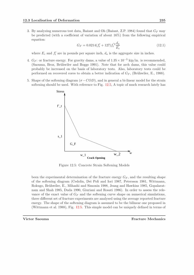
12.3 Localisation of Deformation 235
3. By analyzing numerous test data, Bazant and Oh (Bazant, Z.P. 1984) found that GF maybe predicted (with a coefficient of variation of about 16%) from the following empiricalequation:
GF = 0.0214(f ′t + 127)f
′2t
da
Ec(12.1)
where Ec and f ′t are in pounds per square inch, da is the aggregate size in inches.
4. GF : or fracture energy. For gravity dams, a value of 1.35×10⁻³ kip/in. is recommended,(Saouma, Broz, Bruhwiler and Boggs 1991). Note that for arch dams, this value couldprobably be increased on the basis of laboratory tests. Also, laboratory tests could beperformed on recovered cores to obtain a better indication of GF , (Bruhwiler, E., 1988).
5. Shape of the softening diagram (σ−COD), and in general a bi-linear model for the strainsoftening should be used. With reference to Fig. 12.5, A topic of much research lately has
f’_t
w
G_F
w_1
s_1
w_2Crack Opening
Stress
Figure 12.5: Concrete Strain Softening Models
been the experimental determination of the fracture energy GF , and the resulting shapeof the softening diagram (Cedolin, Dei Poli and Iori 1987, Petersson 1981, Wittmann,Rokugo, Bruhwiler, E., Mihashi and Simonin 1988, Jeang and Hawkins 1985, Gopalarat-nam and Shah 1985, Duda 1990, Giuriani and Rosati 1986). In order to assess the rele-vance of the exact value of GF and the softening curve shape on numerical simulations,three different set of fracture experiments are analysed using the average reported fractureenergy. The shape of the softening diagram is assumed to be the bilinear one proposed in(Wittmann et al. 1988), Fig. 12.5. This simple model can be uniquely defined in terms of
Victor Saouma Fracture Mechanics

236 FRACTURE DETERIORATION ANALYSIS OF CONCRETE
the tensile strength f ′t, and the fracture energy GF . In (Bruhwiler and Wittmann 1990a),
it was found that the optimal points for concrete with 1” maximum size aggregate are:
s1 = 0.4f ′t (12.2)
w1 = 0.8GF
f ′t
(12.3)
w2 = 3GF
f ′t
(12.4)
whereas for structural concrete, (Wittmann et al. 1988), the corresponding values are:
s1 =f ′
t
4(12.5)
w1 = 0.75GF
f ′t
(12.6)
w2 = 5GF
f ′t
(12.7)
where f ′t is the uniaxial tensile strength. Within the context of a nonlinear fracture
mechanics analysis, this tensile strength can not be taken as zero, otherwise there will beno fracture process zone. As f ′
t is seldom determined experimentally, it is assumed to be9% of f ′
c, (Mindess and Young 1981).
6. In lieu of a direct tension test, a flexural test can be performed under strain control,and the fracture energy GF could still be determined from the area under the load andcorresponding displacement curve.
7. For dynamic analysis, the fracture properties of dam concrete depend on both rate ofloading and preloadings. Test results (Bruhwiler and Wittmann 1990a) show that thefracture properties generally increase with increasing loading rate. However, dynamiccompressive preloading leads to a reduction of the fracture properties at both quasi-staticand high loading rates.
12.3.2 Theoretical Evidence
12.3.2.1 Static Loading
22 Let us consider a simple bar loaded in uniform tension and made up of m elements, Fig.12.6.
23 Prior to reaching the peak stress ft, we have a linear stress strain relationship σ = Eε.
24 Once the peak load is reached, the concrete softens and the peak strain is εu. At that pointthe load carrying capacity of the bar is exhausted.
Victor Saouma Fracture Mechanics

12.3 Localisation of Deformation 237
ft
uε
m=σ
ε
σ
m=n m=2 m=1
m elements
L
u/2ε
Weak Element
L/m1
E
1h
ε0
Figure 12.6: Strain-Softening Bar Subjected to Uniaxial Load
25 The post-peak stress is given by
σ = ft + h(ε − ε0) (12.8)
for degrading (softening) material h (softening modulus) is less than zero, and for linear soft-ening
h = − ft
εu − ε0(12.9)
where ε0 = ft/E.
26 We next assume that one of the elements is weaker than the other m−1 ones. Thus, when thiselement reaches its own tensile strength (lower than ft), it fails. Upon failure of this element,the other ones will simply unload elastically. Thus, in the post-peak zone the displacement willbe
u =L
mεf + (m − 1)
L
mεe (12.10-a)
εf =ft
E+
σ − ft
h(12.10-b)
εe =σ
E(12.10-c)
ε =u
L(12.10-d)
⇒ ε =σ
E+
E − h
Eh
σ − ft
m(12.10-e)
27 The slope of the stress-displacement curve is
u
σ=
(1
E+
E − h
Ehm
)(12.11)
Victor Saouma Fracture Mechanics

238 FRACTURE DETERIORATION ANALYSIS OF CONCRETE
28 If we definen =
εu
ε0(12.12)
then h = −E/(n − 1) and Eq. 12.10-e reduces to
ε =σ
E+
n(ft − σ)
mE(12.13)
and the post-peak slope isε
σ=
1
E− n
mE(12.14)
29 From Fig. 12.6, we note that depending on the number of element used (m), there is a widerange of possible responses. For m = 1 we have the softening curve reproduced, however form = n we do have a brittle failure. For m = 2 half the bar localizes, and for m > n we wouldhave a strain decrease, i.e. snap-back behavior. This is impossible to achieve experimentally.Physically, that implies that the localization zone can not absorb the elastic energy released bythe elastic part of the bar.
30 If we use an infinite number of elements (m → ∞), then from Eq. 12.13 and 12.14 we notethat we would have an elastic unloading. Physically, this is impossible as it would imply failureoccured without dissipation of energy. As a result we would have:
• Loss of local material stability
• Loss of structural stability
• Loss of ellipticity
• Mesh dependence
31 To illustrate this, let us consider a concrete member subjected to uniaxial load with thefollowing properties: f ′
t = 3 MPa; E =30 GPa; wmax=.02 cm; GF = 12(3×10⁶)(2×10⁻⁴) = 300
N/m. From these properties, the peak strain is εu = 3×10⁶
3×1010 = 10−4 m. Hence, the maximum
elastic displacement is 10−4L. Let us now consider the load displacement curve (P − u) of thismember for various lengths L.
32 In all cases the peak load will be Pmax = 300A where A is the cross sectional area (sinceresults are independent of A we shall assume A=1). The corresponding displacement will begiven by u = εu × L.
33 Similarly, in all cases the maximum displacement will be umax = wmax = .02 cm and thecorresponding load will obviously be equal to zero.
34 The displacement corresponding to the peak load will be equal to wmax if L = wmax
εu=
2×10⁴
10−4 = 2 m. Fig. 12.7 illustrates the load displacement curves in terms of the length L. Thisfigure calls for the following observations:
Victor Saouma Fracture Mechanics

12.3 Localisation of Deformation 239
0.000 0.010 0.020 0.030 0.040Displacement u (inch)
0.0
100.0
200.0
300.0
Load
(Lb
s)
L=10 in.L=100 in.L=200 inL=300 in.L=400 in.
Figure 12.7: Load Displacement Curve in terms of Element Size
Victor Saouma Fracture Mechanics

240 FRACTURE DETERIORATION ANALYSIS OF CONCRETE
L (m) 0.1 1. 2. 3. 4.UA 15. 150. 300. 450. 600.
Table 12.1: Strain Energy versus Fracture Energy for uniaxial Concrete Specimen
1. Specimens less than 2 m long do exhibit a softening branch which can be experimentallyobtained only through displacement controlled tests.
2. For a 2 m specimen, we do have a perfectly brittle response.
3. For specimens larger than 2 m, there is a snapback, which can only be hypothesized butnot experimentally obtained.
4. Large specimens could still be tested, however rather than using the entire specimen lengthas “gage length” (or displacement/stroke control test), we would have to use a smaller gagelength (through strain control tests) across a potential crack. Thus a notched specimenshould be used.
35 In summary, the load displacement curve of this simple test is clearly size dependent. Thelarger the specimen, the larger the stored strain energy which would be released to form surfaceenergy.
36 An energetic interpretation of this figure would lead us to compare the elastic energy U =12f ′
tεuAL = 12(3×10⁶)(10−4)AL = 150AL at peak load with the fracture energy GF = 300 N/m.
As long as the strain energy is smaller than the fracture energy, then we do have structuralsoftening; if the two energies are equal, then we would have a perfectly brittle response; finally,if the elastic energy exceeds the fracture energy, then we would have a sudden failure withsnap-back. Table 12.1 tabulates those energy values.
37 Again we observe that UA = GF for L = 200 inches. Thus, as long as the energy released
can be transformed into fracture energy, we do have a stable configuration. However if theaccumulated strain energy being released (including not only the one stored in the specimen,but also in the experimental set-up) is greater than the one which can be absorbed to createnew surface energy (cracks), then we do have instability.
38 This simple exercise can be generalized to the analysis of simple tensile structures in whichelements are either perfectly brittle and/or softening.
39 Finally, and as a minor remark, for a successful post-peak experiment the total strain energy(of the specimen and of the testing frame) should be less than the fracture energy. Hence, toavoid snap-backs the testing frame should be as stiff as possible.
12.3.2.2 Dynamic Loading
Adapted from (Sluys 1992)
Victor Saouma Fracture Mechanics

12.3 Localisation of Deformation 241
12.3.2.2.1 Loss of Hyperbolicity
40 We can write the dynamic equilibrium of a system along the x axis as
ρ∂2u
∂t2=
∂σxx
∂x+
∂σxy
∂y+
∂σxz
∂z(12.15)
For a uniaxial state of stress, and with σxx = f(εxx), this equation reduces to
c2 ∂2u
∂x2=
∂2u
∂t2(12.16)
where c2 = 1/ρ∂f∂ε and is the square of the speed of the wave propagation. Equation 12.16 is the
classical wave equation of motion (hyperbolic equation). D’alembert’s solution of this equationis of the form
u = f(x + ct) + g(x − ct) (12.17)
and a real solution exists as long as ∂f/∂ε ≥ 0. Thus, in a softening regime where ∂f/∂ε < 0,the speed of wave propagation becomes complex and the problem is thus ill-posed. We thushave a loss of hyperbolicity.
12.3.2.2.2 Wave Equation for Softening Maerials
41 Considering
Equation of Motion: ρ∂2u
∂t2=
∂σ
∂x(12.18-a)
Kinematic Equation: ε =∂u
∂x(12.18-b)
Constitutive Equation: σ = fε (12.18-c)
where u is the velocity v, and the strain can be decomposed into an elastic and inelasticcomponent.
ε = εe + εi (12.19)
and thusσ = f ′εi (12.20)
where f ′ denotes differentiation with respect to the inelastic strain,
42 Taking εe = σ/E, the x derivative of the preceding equation yields
∂σ
∂x= f ′∂εi
∂x(12.21-a)
Victor Saouma Fracture Mechanics

242 FRACTURE DETERIORATION ANALYSIS OF CONCRETE
= f ′[∂ε
∂x− ∂εe
∂x] (12.21-b)
= f ′[∂2u
∂x2− 1
E
∂σ
∂x] (12.21-c)
⇒ ∂σ
∂x=
f ′EE + f ′
∂2v
∂x2(12.21-d)
43 Substituting this equation into Eq. 12.18-a we obtain the wave equation for a one-dimensionalstrain-softening element
f ′ + E
c2e
∂2v
∂t2− f ′ ∂
2v
∂x2= 0 (12.22)
where ce =√
E/ρ is the linear elastic longitudinal wave velocity. This equation should becontrasted with Eq. 12.16 for the elastic solids.
44 One way to solve this second order partial differential equation (linear only if f ′ is constant)is to consider the variation of the first derivative of the velocity v with respect to both x and t
d
(∂v
∂t
)=
∂2v
∂t2dt +
∂2v
∂x∂tdx = 0 (12.23-a)
d
(∂v
∂x
)=
∂2v
∂x2dx +
∂2v
∂x∂tdt = 0 (12.23-b)
45 Combining the last three equations together yields a system of three second order differentialequations ⎡
⎢⎣ (E + f ′)/c2e 0 −f ′
dt dx 00 dt dx
⎤⎥⎦⎧⎪⎨⎪⎩
∂2v∂t2∂2v∂x∂t∂2v∂x2
⎫⎪⎬⎪⎭ = 0 (12.24)
46 The characteristic determinant is∣∣∣∣∣∣∣(E + f ′)/c2
e 0 −f ′
dt dx 00 dt dx
∣∣∣∣∣∣∣ =E + f ′
c2e
dx2 − f ′dt2 = 0 (12.25)
If the determinant is equal to zero, then a solution for the curve in the x − u − t plane shouldcoincide with the characteristic direction.
dx
dt= ±ce
√f ′
E + f ′ (12.26)
47 In a wave equation, the characteristic (±dx/dt) coincides with the wave speed (±c). In caseof softening (f ′ < 0) and if we have snap-through (f ′ > −E), then the characteristics and
Victor Saouma Fracture Mechanics

12.4 Griffith Criterion and FPZ 243
therefore the wave speeds are imaginary. This results in a loss of hyperbolicity into ellipticitywhenever softening occurs.
48 We thus have a domain governed by hyperbolicity, and another one by ellipticity where thewave can not propagate. Spatial interaction between the two is impossible, and we have anill-posed problem.
49 A strain-softening material is thus non-dispersive. In a dispersive media, harmonic waveswith different frequency propagate with different wave speeds.
50 Assuming that we have a single linear harmonic wave propagation
v(x, t) = Aei(kx−ωt) (12.27)
where ω is the angular frequency, k = 2π/λ the wave number. Substituting Eq. 12.27 into12.22 we obtain
ω = ce
√f ′
E + f ′k (12.28)
The wave velocity being equal to
cf =ω
k(12.29)
it is now apparent that in a softening material c = cf is independent of k and is thereforenon-dissipitative, thus all the waves would have the same imaginary speed.
51 For proper description of localisation, wave propagation must be dispersive.
12.3.3 Conclusion
In summary, Fig. 12.8 illustrates the localization of strain in a plate subjected to uniformtensile deformation.
12.4 Griffith Criterion and FPZ
52 Let us consider a cohesive crack with both normal and tangential tractions in a thin platesubjected to far field stresses, and let us assume the crack is to be under general mixed modeconditions, Figure 23.16.
53 To verify if the non-linear model satisfies Griffith criterion, it is necessary to compute theenergy released by a unit crack propagation. The J-integral provides a method to evaluate theenergy release rate. The J-integral is a path independent integral and in two-dimensional isgiven by:
J =
∮Γ(Wnx − t
∂u
∂x)dΓ (12.30)
Victor Saouma Fracture Mechanics
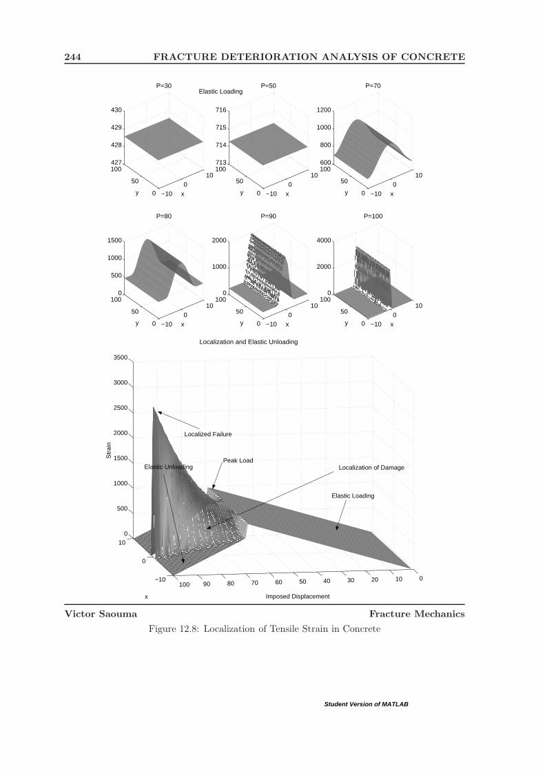
244 FRACTURE DETERIORATION ANALYSIS OF CONCRETE
−100
10
0
50
100427
428
429
430
xy
P=30
−100
10
0
50
100713
714
715
716
xy
P=50
−100
10
0
50
100600
800
1000
1200
x
P=70
y
−100
10
0
50
1000
500
1000
1500
x
P=80
y −100
10
0
50
1000
1000
2000
x
P=90
y −100
10
0
50
1000
2000
4000
x
P=100
y
Elastic Loading
Localization and Elastic Unloading
Student Version of MATLAB
−10
0
10
0102030405060708090100
0
500
1000
1500
2000
2500
3000
3500
Imposed Displacementx
Str
ain
Elastic Loading
Elastic Unloading Peak Load
Localized Failure
Localization of Damage
Student Version of MATLAB
Figure 12.8: Localization of Tensile Strain in Concrete
Victor Saouma Fracture Mechanics

12.4 Griffith Criterion and FPZ 245
Γ
σ
τ
στ
Γ0
στ
Figure 12.9: Griffith criterion in NLFM.
54 Due to its path independent character it is possible to evaluate the J-integral along the cracksurfaces where nx = 0.
J(Γo) = −∫Γo
t∂u
∂xds =
∫FPZ
(τ∂u
∂x+ σ
∂v
∂x
)dx (12.31)
55 Applying Leibnitz rule for the differentiation of definite integrals1 the J-integral is equivalentto:
J(Γo) =
∫FPZ
[d
dx
(∫ u
0τ du
)]dx +
∫FPZ
[d
dx
(∫ v
0σ dv
)]dx (12.32)
56 The expressions in parentheses represent the surface energies dissipated in mode I and II atevery point along the fracture process zone normalized with respect to crack surface.
57 Hence, we define: ∫ u
0τ du = qII(x),
∫ v
0σ dv = qI(x) (12.33)
J(Γo) =
∫FPZ
dqII(x)
dxdx +
∫FPZ
dqI(x)
dxdx = GII
c + GIc = Gc (12.34)
where GIIc and GI
c is the energy dissipated by a unit propagation of the cohesive crack in modeII and I respectively.
58 It should be noted that in general, GIIc and GI
c are not equivalent to GIIF and GI
F , but arerather functions of these and the stress state along the interface. However, it is possible toconsider two special cases for pure mode I and II cracks.
1 d
dt
∫ b
af(x, t)dx =
∫ b
a
∂f
∂t(x, t)dx; In other words, differentiation and integration can be interchanged.
Victor Saouma Fracture Mechanics

246 FRACTURE DETERIORATION ANALYSIS OF CONCRETE
59 In the case of pure mode I crack, the J-integral is equal to:
J(Γo) =
∫FPZ
[d
dx
(∫ v
0σ dv
)]dx =
∫ wσ
0σ(v) dv = GI
F (12.35)
60 Similarly, in the case of pure mode II crack, the J-integral is equal to:
J(Γo) =
∫FPZ
[d
dx
(∫ u
0τ du
)]dx =
∫ wτ
0τ(u) du = GII
F (12.36)
where wσ and wτ is the critical crack opening and sliding respectively for which normal andtangent stresses can no longer be transferred across the crack.
61 The following conclusion, can be drawn based on the basis of the previous discussion:
1. It was shown that a unit extension of a cohesive crack model dissipates energy whoseamount depends on the softening laws used by the model. The amount of dissipatedenergy also depends on the loading conditions in FPZ. In pure mode I and mode II loading,specific fracture energies GI
F and GIIF are dissipated respectively. If the structural system
cannot provide these energies, the crack would not propagate.
2. In the limiting case, when the dimensions of the analyzed problem increase, the cohesivecrack gives identical results as LEFM.
3. In finite element implementation, errors are introduced due to discretization errors. Inlarge structures, fine mesh would be necessary at the crack tip to model the fractureprocess zone. If the FPZ is not modeled adequately, the Griffith criterion for crackpropagation is violated, and erroneous results will be obtained.
Victor Saouma Fracture Mechanics

Chapter 13
FRACTURE MECHANICS ofCONCRETE
13.1 Fracture Toughness Testing of Concrete: a Historical Per-
spective
Section adapted from ACI Committee 446 (2003)
1 ACI Committee 446 (1991) describes various methods for fracture toughness testing of con-crete, summarized and extended briefly here.
2 Kaplan (1961), assuming LEFM conditions prevail, was the first to attempt to determine thefracture toughness of concrete. Subsequent analysis in the 1970s and early 1980s showed thatLEFM was not an appropriate model for fracture of concrete (Walsh 1972), (Walsh 1976), and(Swartz, Hu, Fartash and Huang 1982)). In retrospect, now knowing that the fracture processzone may be very long, we understand why LEFM is inapplicable.
3 Many attempts have been made to measure the fracture toughness of concrete using beams,assuming the existence of an effective LEFM crack. These include various compliance calibra-tion methods applied to beams (Swartz, Hu and Jones 1978), (Swartz and Go 1984), (Swartzand Refai 1989) (Jenq and Shah 1985).
4 Wedge splitting tests on various compact tension specimens have also been proposed (Linsbauerand Tschegg 1986), (Bruhwiler, E., 1988), (Bruhwiler and Wittmann 1990b), (Bruhwiler, E.,Broz, J.J., and Saouma, V.E., 1991), (Bruhwiler, E., and Saouma, V.E., 1990). The apparentfracture toughness, KIc, or more properly, KQ, is obtained by the same method as described infor notched beam tests. The effective crack length, which accounts for the fracture process zone,is determined by the compliance method, based on finite element calibration. For that purpose,unload-reload cycles are performed during the test. Other methods such as the evaluation offracture energy from the area under the load-displacement diagram and the size effect methodare more applicable, as described next.

248 FRACTURE MECHANICS of CONCRETE
5 An effective LEFM crack method based on the work of Nallathambi and Karihaloo (1986)has been proposed to RILEM as a standard, (Karihaloo and Nallathambi 1987).
6 The work of fracture method, originally developed for ceramics (Nakayama 1965), (Tattersalland Tappin 1966), is the first method of testing for fracture properties of concrete to be proposedas a standard (RILEM Committee on Fracture Mechanics of Concrete - Test Methods 1985).The basis for applying this method to concrete was developed by Hillerborg and his co-workers,(Hillerborg 1985b). Their method is based upon the cohesive crack model. The method canbe applied to a variety of test specimen geometries but the proposed standard uses a beamspecimen loaded in three-point bending with a central edge notch.
7 In summary, the RILEM work-of-fracture method is a practical approach, which is suitablefor use in laboratories that do not have very elaborate equipment. The method incorporates anumber of compromises in order to simplify testing while still obtaining useful results (Hillerborg1985b). The method is based on a theory that has gained wide acceptance, the cohesive crackmodel (Hillerborg, A. and Modeer, M. and Petersson, P.E. 1976b). The fracture energy methodis conceptually simple, requiring no LEFM assumptions.
8 Round-robin tests from 14 laboratories incorporating about 700 beams were reported byHillerborg (1985a). With regard to variation of results within a given tests series, the coefficientof variation ranged from about 2.5% to 25% with most results around 10 to 15%.
9 There are, however, certain aspects in which the RILEM work-of-fracture method requiresimprovement. The size dependence of fracture energy GRf obtained according to the existingRILEM recommendation on the work of fracture method has been investigated by Planas andElices (1988b) and Planas and Elices (1988a) on the basis of solution of an integral equationand by Bazant, Z.P. and Kazemi, M.T. (1990) on the basis of the size effect law.
10 The RILEM work-of-fracture method does not give results independent of the size of thecracked area for a given beam depth, and thus the value of GRf is only an approximation of thetrue energy parameter which characterizes the surface energy and the energy of process zoneformation. Furthermore, the work-of-fracture method gives only one parameter, GRf , whichis a lower bound on the true fracture energy of the concrete. Also, the true fracture energy,GF , may not be the most important parameter in design; rather Gf (the area under the initialportion of the cohesive -COD curve may be more important).
11 The size effect method has also been proposed as the basis for a fracture toughness teststandard, (Bazant and Kazemi 1990), (Bazant and Pfeiffer 1987), (Karihaloo and Nallathambi1987). This method is appealing in that only peak loads need be determined; no displacementmeasurements are required. However, after some testing and analysis, it has been determinedthat to develop a fracture toughness test method based upon the size effect would (arguably)require an unreasonably wide range of specimen sizes, with required specimen sizes too largeto be practical.
12 A stiff direct tension test performed on a standard 6 inch diameter by 12 inch long cylinder
Victor Saouma Fracture Mechanics

13.2 Nonlinear Fracture Models 249
to obtain the cohesive crack ( -COD) relationship has been proposed by Lenke and Gerstle(2001), who have proposed a test standard based upon their work.
13.2 Nonlinear Fracture Models
13.2.1 Models
13.2.1.1 Cohesive Crack Model
13 The cohesive crack model of Hillerborg, is by far the most important and widely used model.It has already been discussed in Sect. ??sect:hillerborg-model.
13.2.1.2 Jenq and Shah Two Parameters Model
14 To circumvent the problems associated with nonlinear fracture, and combing the effectivecrack length proposed by Irwin (one which takes into account the plastic zone) with the CTODcriteria, Jenq and Shah (1985) have introduced a two-parameter-model. To introduce thismodel, let us first consider the load CMOD (crack mouth opening displacement) of a notchedspecimen. From this diagram the following three stages can be identified:
1. Linear elastic response up to a load corresponding approximately to Pcr
2. . That is, the
induced LEFM KI is less than KIc
2. . During this stage the CTOD (crack tip openingdisplacement) is zero as predicted by LEFM.
2. During the second stage, significant inelastic deformation takes place. This is causedby the formation of the process zone ahead of the crack tip (the existing crack beingprenotched or precast, and not the result of some prior crack nucleation/extension, forwhich a process zone first has to be developed). This process zone formation has also beenreferred to as slow crack growth. As a result of this microcracking the crack tip starts toopen in a fashion similar to the blunting of sharp cracks in metals due to yielding.
3. At the peak load, and for unstable geometries (i.e., increasing KI with increasing cracklength a), we have two conditions that are simultaneously satisfied:
KI = KSIc (13.1)
CTOD = CTODc (13.2)
where the right hand side values are now considered material properties, and the CTODrefers to the notch opening (and not crack) opening.
15 Thus in this simple, clear, and elegant model we implicitly account for softening by in-troducing a second parameter (CTOD), whereas in Hillerborg’s approach the SIF concept isentirely discarded and replaced by a fictitious load, the distribution of which requires at leasttwo parameters.
Victor Saouma Fracture Mechanics

250 FRACTURE MECHANICS of CONCRETE
16 This model has been shown to yield results that are specimen size insensitive. A minordrawback of this model is that it requires an analytical expression of the COD and KI alongthe crack for the geometry considered. In most cases this entails a finite element calibration.
17 This model requires an analytical expression for KI and the CTOD along the crack foreach geometry considered, which in most cases can only be obtained through a finite elementcalibration. The model distinguishes between notch and crack length, and CTODc is evaluatedat the notch, thus the nonzero value for CTODc. Based on an extensive test program, thecritical values, KS
Ic and CTODc, were found to be size-independent material properties.
13.2.2 Characteristic Lengths
13.2.2.1 Hillerborg
18 Associated with this model is the characteristic length, lch, also proposed by Hillerborg, A.and Modeer, M. and Petersson, P.E. (1976a) in 1976 and which is a material property whichgives an indication of the material brittleness, and is defined as:
lch =EGF
f′2t
(13.3)
where, E is Young’s Modulus, f ′t is the tensile strength, and GF is the specific fracture energy.
This equation should be compared with Irwin’s plastic zone size Eq. 8.9
rp =1
π
K2I
σ2yld
=GE
σ2yld
(13.4)
19 Hillerborg, A. and Modeer, M. and Petersson, P.E. (1976a) and Hillerborg, A. (1983) haveshown that the ratio of structural dimension, d, to characteristic length, lch, is the dominantparameter for describing size effects using the Fictitious Crack Model (FCM). LEFM is con-sidered to be applicable for large values of d
lch. Analysis of three point bending beams, where
d is the beam depth, (Hillerborg, A. 1985) and of compact tension specimens, where d is thespecimen height, (Bruhwiler, E. and Roelfstra, P.E., 1989) showed that LEFM may not be validfor d/lch < 25, and that a ratio of d
lch= 25 would result in a 5% difference between the load
carrying capacities predicted by LEFM and FCM.
13.2.2.2 Jenq and Shah
20 Finally, when combined with Young’s Modulus, E, a single fracture parameter describingthe material, termed the critical material length, Q, was derived:
Q =
(E · CTODc
KSIc
)2
(13.5)
The Q-value is related to the brittleness of the specimen. For large Q-values the materialexhibits a high brittleness.
Victor Saouma Fracture Mechanics
13.2 Nonlinear Fracture Models 251
13.2.2.3 Carpinteri Brittleness Number
21 In fracture testing, failure may be caused by different mechanisms: (1) ultimate strengthcollapse (SOM), and, (2) fracture collapse in terms of LEFM. The dimensionless brittlenessnumber, s, was developed by Carpinteri to assess the existence of either one of the two failuremechanisms (Carpinteri 1982a), (Carpinteri 1982b), (Carpinteri 1986). This parameter dependson the fracture toughness, KIc, the tensile strength, f ′
t, and on a dimension d characteristic ofthe specimen (or structure) geometry being considered:
s =KIc
f ′t
√d
(13.6)
22 For large brittleness numbers, i.e., small specimen dimension d, SOM governs, and the in-terpretation of tests through Fracture Mechanics (FM) is not valid. Conversely, for smallbrittleness numbers, fracture mechanics is applicable since the specimen is more brittle. Theboundary between SOM and FM applicability, is defined by the critical brittleness number, s0,which is obtained from the nominal stress at failure.
13.2.3 Comparison of the Fracture Models
This section is taken from (Bruhwiler, E., Broz, J.J., and Saouma, V.E., 1991)
23 All models considered in this chapter are used to assess the brittleness and by consequence theapplicability of LEFM. Because the models originate from different, but related, formulationsdescribing identical physical phenomena, i.e., tensile softening of concrete and its size effects,this section will analytically show the similarity between them. Similar studies have beenreported by Planas and Elices (Planas and Elices 1988b).
24 They showed in a numerical analysis that, over limited ranges, existing fracture modelsmay be thought as approximations of one another in a mathematical sense and experimentallyindistinguishable, based on size effect alone. First the relationship between Hillerborg’s modeland Griffith’s LEFM model is rederived, and then all subsequent ones are found to be a variationof this model.
13.2.3.1 Hillerborg Characteristic Length, lch
25 Hillerborg’s characteristic length, lch, can be traced back to the fundamental equation gov-erning linear elastic fracture mechanics (Hillerborg 1985a):
KIc = β · σcr√
πacr (13.7)
where σcr and acr are critical stress and crack length, respectively, and β is a correction factoraccounting for specimen geometry, boundary, and loading conditions. The fracture toughness
Victor Saouma Fracture Mechanics

252 FRACTURE MECHANICS of CONCRETE
KIc in turn can then be related to the critical energy release rate Gc as derived by Irwin (1957),
Gc =K2
Ic
E′ (13.8)
where,
E′ =
{E : for plane stress
E(1−ν2) : for plane strain
(13.9)
26 Since concrete has a low Poisson’s ratio ν, plane stress is primarily considered, and for“large” concrete structures in which LEFM is applicable, the strain energy release rate Gc
becomes equal to GF . Thus Eqs. 13.7 and 13.8 can be rewritten as:
EGF = β2σ2crπacr (13.10)
27 Hillerborg’s characteristic length is then obtained with σcr = f ′t, or:
EGF
f ′t2 = β2πacr = lch (13.11)
Eq. 13.11 shows that the critical crack size is of the same order of magnitude as the characteristiclength lch, which, for a given specimen geometry, may be approximately proportional to thelength of the fracture process zone.
13.2.3.2 Bazant Brittleness Number, β
28 The intersection between the SOM and LEFM approaches in the size effect diagram (Fig.14.10) where
σLEFMN = σSOM
N (13.12)
defines the point where the brittleness number, β is equal to 1, or d = λ0da = d0. From
KIc = DPmax
t · d√
d (13.13)
Pmax
td=
KIc
D√
d0(13.14)
and combining withPmax
t · d =σN
C(13.15)
we obtainPmax
td=
Bf ′t
C(13.16)
Eqs. 13.14 and 13.16 are combined into one equation, yielding:
f ′t2d0
K2Ic
=
(C
BD
)2
= K2 (13.17)
Victor Saouma Fracture Mechanics

13.2 Nonlinear Fracture Models 253
29 Because LEFM is assumed valid, substituting K2Ic with GF · E (Eq. 13.8), leads to:
f ′t2d0
GF E=
d0
lch= K2 (13.18)
30 Thus, the brittleness number β used to assess the applicability of LEFM in the Size EffectLaw can be related to Hillerborg’s characteristic length, lch. Eq. 13.18 indicates that d/lchhas a similar significance to the ratio between structural dimension d and maximum aggregatesize da in the Size Effect Law. Since lch is a comprehensive parameter to describe materialfracture, the d/da ratio in the Size Effect Law may be replaced by d/lch (Bruhwiler, E., 1988).Comparison between the Size Effect Law and the Fictitious Crack Model showed that bothmodels yield good agreement in the prediction of the size effect (Hillerborg, A. 1985) and (?).
13.2.3.3 Carpinteri Brittleness Number, s
31 Squaring the expression s of the brittleness number (Eq. 13.6), and assuming that K2Ic =
E · GF , when LEFM is valid, the following expression is obtained:
s2 =EGF
f ′t2d
=lchd
(13.19)
or
s =
√lchd
(13.20)
13.2.3.4 Jenq and Shah’s Critical Material Length, Q
32 In the Fictitious Crack Model, the area under the softening law, relating the tensile stress,σ, to fictitious crack width, w, is defined as the specific fracture energy, GF , or:
GF = Cf ′t · wc (13.21)
where, C is a constant characterizing the σ vs. w curve, and wc is the crack width for which σ= 0. At the tip of the real crack (or notch) in the FCM, wc can be interpreted as the criticalcrack tip opening displacement, CTODc, according to the Two-Parameter Model. Therefore,CTODc is set equal to wc, and Eq. 13.21 can be rewritten as:
CTODc =GF
Cf ′t
(13.22)
Combining Q (Eq. 13.5) with Eq. 13.22:
Q =E2G2
F
KIc2C2f ′
t2 (13.23)
With K2Ic = GF E, Q is finally related to lch:
Q =EGF
C2f ′t2 =
lchC2
(13.24)
Victor Saouma Fracture Mechanics

254 FRACTURE MECHANICS of CONCRETE
13.2.3.5 Discussion
33 Table 13.1 summarizes the preceding analysis of models and indicates that all models are
Table 13.1: Summary relations for the concrete fracture models.
Author Hillerborg Carpinteri Jenq & Shah Bazant
Year 1976 1982 1985 1984
Parameter lch s Q d0
Relation lch = EGF
f ′
t2 s =
√lch
d Q = lch
C2 d0 = K2lch
related to Hillerborg’s characteristic length, and thus related to Griffith’s model. Althoughrelations among all the models have been demonstrated, differences in experimental resultsare due to the initial assumptions of very large concrete structures, where LEFM is valid, i.e.,
Gc =K2
Ic
E′ and Gc = GF . Yet, the results of the comparisons indicate a unified approach couldpossibly be postulated. Validation of such an approach in the laboratory would prove difficultdue to specimen size considerations.
13.2.4 Model Selection
34 In light of the diversity of models, Engineers should exercise great care in selecting an ap-propriate model. Model selection should account for:
1. Crack size: In a “large” crack, the effect of the process zone is smaller than for a “short”one. Thus LEFM is more applicable for the large ones.
2. Type of loading: If a structure is subjected to a load rather than imposed displacements(such as foundation settlements), than only a pre-peak response is of importance. Underthose conditions non-linear effects may be negligible compared to the ones induced byLEFM.
3. Stability1: In a structure subjected to imposed load rather than imposed displacementnon-linear effects are not be as negligible in a stable structure as they are in an unstableone.
Thus Table 13.2 provides some guidance for model selection. Accordingly we should select:
1. An NLFM for an arch dam which cracking is caused by foundation settlement.
2. An LEFM model for a dam in which cracking is caused by flooding, no matter how smallor large the crack is.
Victor Saouma Fracture Mechanics

13.3 Fracture Energies Gf and GF 255
Loading “Small” Crack “Large” Crack
Load Control, Unstable LEFM LEFMLoad Control, Stable NLFM LEFM
Displacement Control NLFM LEFM
Table 13.2: When to Use LEFM or NLFM Fracture Models
35 In all cases, it should be emphasized that ideally a non-linear analysis is to be undertaken,however in many (but not all) cases the complexity and expenses associated with such ananalysis yield results very close to the ones obtained from a linear elastic ones. Thus ultimatelythe type of analysis to be undertaken hinges on both technical and economical considerations.
36 Amongst the competing models for NLFM, the one recommended, and by far the most widelyused, is the one based on the Cohesive Crack Model (CHM).
13.3 Fracture Energies Gf and GF
Section adapted from (Bazant, Yu and Zi 2002)
37 One essential parameter of the cohesive (or fictitious) crack model is the tensile strength ofthe material, f ′
t. The softening stress-separation curve of the cohesive crack model (Hillerborg etal. 1976, Petersson 1981, Hillerborg 1983, 1985a,b), is usually characterized by two parameters.They can be chosen as either
1. f ′t and fracture energy GF , representing the area under the complete curve (Rice 1969,
Hillerborg et al. 1976, Petersson 1991, Hillerborg 1983, 1985a,b), or
2. f ′t and fracture energy Gf , representing the area under the initial tangent of the softening
curve, (Elices, Guinea and Planas 1992).
38 The fracture energies Gf and GF are two different material characteristics which are onlypartially correlated. GF can be estimated from Gf and vice versa, but not accurately. Ideally,both Gf and GF should be measured and used for calibrating the initial slope and the tail ofthe softening curve of the cohesive crack model (or crack band model), which are both neededfor fracture analysis of structures.
39 For concrete, as a rough approximation
GF ≈ 2.5Gf (13.25)
as reported by Planas and Elices (1992) and further verified by Bazant and Becq-Giraudon(2001). Knowing this ratio, one can calibrate a bilinear softening curve, provided that the
1A stable structure is one in which KI decreases with crack length, in an unstable one the stress intensityfactor KI increases with crack length.
Victor Saouma Fracture Mechanics
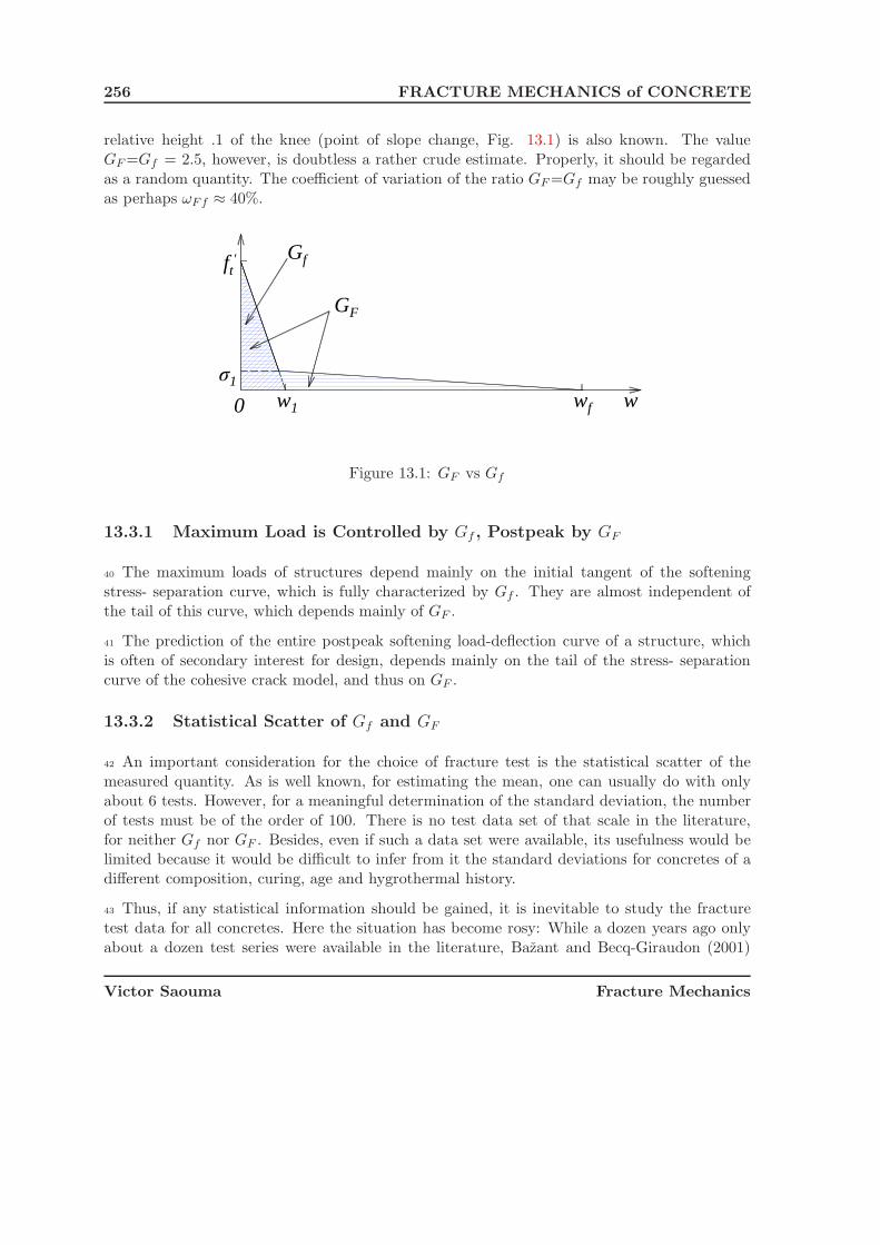
256 FRACTURE MECHANICS of CONCRETE
relative height .1 of the knee (point of slope change, Fig. 13.1) is also known. The valueGF =Gf = 2.5, however, is doubtless a rather crude estimate. Properly, it should be regardedas a random quantity. The coefficient of variation of the ratio GF =Gf may be roughly guessedas perhaps ωFf ≈ 40%.
ft'
σ1
0 w1 wf w
Gf
GF
Figure 13.1: GF vs Gf
13.3.1 Maximum Load is Controlled by Gf , Postpeak by GF
40 The maximum loads of structures depend mainly on the initial tangent of the softeningstress- separation curve, which is fully characterized by Gf . They are almost independent ofthe tail of this curve, which depends mainly of GF .
41 The prediction of the entire postpeak softening load-deflection curve of a structure, whichis often of secondary interest for design, depends mainly on the tail of the stress- separationcurve of the cohesive crack model, and thus on GF .
13.3.2 Statistical Scatter of Gf and GF
42 An important consideration for the choice of fracture test is the statistical scatter of themeasured quantity. As is well known, for estimating the mean, one can usually do with onlyabout 6 tests. However, for a meaningful determination of the standard deviation, the numberof tests must be of the order of 100. There is no test data set of that scale in the literature,for neither Gf nor GF . Besides, even if such a data set were available, its usefulness would belimited because it would be difficult to infer from it the standard deviations for concretes of adifferent composition, curing, age and hygrothermal history.
43 Thus, if any statistical information should be gained, it is inevitable to study the fracturetest data for all concretes. Here the situation has become rosy: While a dozen years ago onlyabout a dozen test series were available in the literature, Bazant and Becq-Giraudon (2001)
Victor Saouma Fracture Mechanics
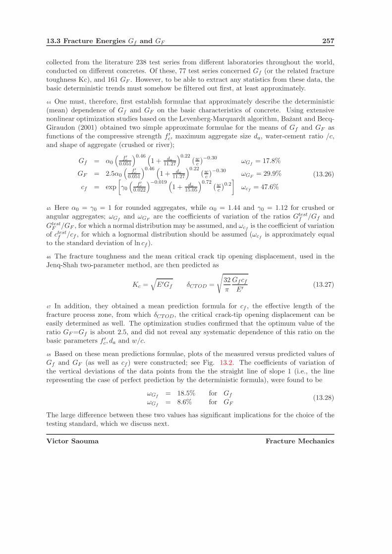
13.3 Fracture Energies Gf and GF 257
collected from the literature 238 test series from different laboratories throughout the world,conducted on different concretes. Of these, 77 test series concerned Gf (or the related fracturetoughness Kc), and 161 GF . However, to be able to extract any statistics from these data, thebasic deterministic trends must somehow be filtered out first, at least approximately.
44 One must, therefore, first establish formulae that approximately describe the deterministic(mean) dependence of Gf and GF on the basic characteristics of concrete. Using extensivenonlinear optimization studies based on the Levenberg-Marquardt algorithm, Bazant and Becq-Giraudon (2001) obtained two simple approximate formulae for the means of Gf and GF asfunctions of the compressive strength f ′
c, maximum aggregate size da, water-cement ratio /c,and shape of aggregate (crushed or river);
Gf = α0
(f ′
c
0.051
)0.46 (1 + da
11.27
)0.22 (wc
)−0.30ωGf
= 17.8%
GF = 2.5α0
(f ′
c
0.051
)0.46 (1 + da
11.27
)0.22 (wc
)−0.30ωGF
= 29.9%
cf = exp
[γ0
(f ′
c
0.022
)−0.019 (1 + da
15.05
)0.72 (wc
)0.2]
ωcf= 47.6%
(13.26)
45 Here α0 = γ0 = 1 for rounded aggregates, while α0 = 1.44 and γ0 = 1.12 for crushed orangular aggregates; ωGf
and ωGFare the coefficients of variation of the ratios Gtest
f /Gf and
GtestF /GF , for which a normal distribution may be assumed, and ωcf
is the coefficient of variationof ctest
f /cf , for which a lognormal distribution should be assumed (ωcfis approximately equal
to the standard deviation of ln cf ).
46 The fracture toughness and the mean critical crack tip opening displacement, used in theJenq-Shah two-parameter method, are then predicted as
Kc =√
E′Gf δCTOD =
√32
π
Gf cf
E′ (13.27)
47 In addition, they obtained a mean prediction formula for cf , the effective length of thefracture process zone, from which δCTOD, the critical crack-tip opening displacement can beeasily determined as well. The optimization studies confirmed that the optimum value of theratio GF =Gf is about 2.5, and did not reveal any systematic dependence of this ratio on thebasic parameters f ′
c, da and w/c.
48 Based on these mean predictions formulae, plots of the measured versus predicted values ofGf and GF (as well as cf ) were constructed; see Fig. 13.2. The coefficients of variation ofthe vertical deviations of the data points from the the straight line of slope 1 (i.e., the linerepresenting the case of perfect prediction by the deterministic formula), were found to be
ωGf= 18.5% for Gf
ωGf= 8.6% for GF
(13.28)
The large difference between these two values has significant implications for the choice of thetesting standard, which we discuss next.
Victor Saouma Fracture Mechanics

258 FRACTURE MECHANICS of CONCRETE
0
25
50
75
100
Gfpr
ed(N
/m)
0 25 50 75 100Gf
pred(N/m)
0 25 50 75 100Gf
pred(N/m)
0
25
50
75
100a) Size Effect and Jenq-
Shah Methodsb) Work-of-Fracture
Method
Figure 13.2: GpredF Based on .....
49 It must, of course, be admitted that the errors of the prediction formulae for Gf and GF ,which are owed to limitations in the understanding of the effect of the differences in concretecomposition, etc., make doubtless large contributions to the aforementioned coefficients of vari-ations. However, there is no reason why these contributions to scatter should be biased infavor one or the other fracture energy. Eliminating the mean trend by an imperfect predictionformula is inevitable if any statistical comparisons at all should be made at the present levelof experimental evidence. Therefore, we must accept that the difference between these twocoefficients of variation characterizes the difference in the random scatter of either Gf and GF ,or their measurement methods, or (more likely) both.
50 Why the data on GF (Fig. 13.2 right) exhibit a much higher scatter than those on Gf?The reasons appear to be: (1) An inherently higher randomness of the tail compared to theinitial portion of the softening curve; (2) uncertainty in extrapolating the tail to zero stress;and (3) difficulties in eliminating energy dissipation not caused by fracture and in achievingindependence of the results from the specimen size (Planas et al., 1992).
51 The fracture parameters measured by the size effect method have the advantage that theyare, by definition, size and shape independent if the correct size effect law for the given sizerange is known.
13.3.3 Level I and Level II Testing
52 At the (pre-FraMCoS-2) workshop of European and American specialists in Cardiff in 1995,organized by B.I.G. Barr and S.E. Swartz, it was agreed that the testing standard should specify
Victor Saouma Fracture Mechanics
13.4 Proposed ACI/ASCE Test Methods 259
two levels of testing:
• At level I, acceptable for structures of not too high fracture sensitivity, one needs tomeasure only one of the two fracture energies, either GF or Gf (a consensus at thatworkshop was to use measurements confined to the maximum load region and ignoringthe tail).
• At level II, appropriate for structures of high sensitivity to fracture and size effect, bothGF and Gf (or Kc instead of Gf ) should be directly measured.
53 If the cohesive crack model is calibrated by a level I test, one must of course assume inadvance the shape of the softening-stress separation curve, i.e., fix the ratios GF =Gf andσknee/f
′t based on prior knowledge. Therefore,
• If GF is measured, one must estimate Gf ≈ 0.4GF , and from that determine the initialslope of the softening curve.
• If Gf is measured, and if the tail of the softening curve is needed, one must estimateGF ≈ 2.5Gf .
13.4 Proposed ACI/ASCE Test Methods
13.4.1 Test 1: Determination of Jenq & Shah Parameters (KIc(tp) And CTODc(tp))
Section adapted from ACI Committee 446 (2003)
54 This test method determines indices of fracture toughness, KIc(tp), critical crack tip openingdisplacement, CTODc(tp) of hardened concrete with maximum aggregate size of 1.33” (3.39 cm)or less.
55 The values of KIc(tp), and CTODc(tp) stated in SI units, are to be regarded as the standard.
56 Supporting references: (Jenq and Shah 1985) (RILEM Committee on Fracture Mechanics ofConcrete-Test Methods 1990) (Guinea, Pastor, Planas and Elices 1998).
13.4.1.1 Terminology
13.4.1.1.1 Definitions
linear elastic fracture mechanics (LEFM) : a theory of fracture mechanics crucial to theunderstanding of this test standard. LEFM assumes linear elastic material behaviortogether with a perfectly sharp crack with traction-free surfaces.
critical effective crack: a conceptual LEFM crack whose length, ac, is selected to providethe same compliance as the observed unloading compliance at or above 95% of peak load.
Victor Saouma Fracture Mechanics

260 FRACTURE MECHANICS of CONCRETE
critical stress intensity factor (KIc(tp)) the stress intensity factor of the critical effectivecrack, calculated using the measured maximum load, Pmax, according to this test stan-dard.
critical crack tip opening displacement (CTODc(tp)) the crack opening displacement cal-culated using LEFM at the original notch tip of the specimen, using the measured maxi-mum load Pmax and the critical effective crack length, ac, according to this test standard.
13.4.1.1.2 Abbreviations
ao initial notch lengthac length of critical effective crackb width of specimenCi initial compliance of specimenCu unloading compliance of the specimenCMOD crack mouth opening displacementCTODc(tp) critical crack tip opening displacement, according to this test standard
d depth of specimenDmax maximum size of coarse aggregateg acceleration of gravityHO thickness of clip gageKIc(tp) critical stress intensity factor, also called fracture toughness, according to
this test standardL length of specimenP load on specimenPmax peak load on specimenS test span of the specimenWo self-weight of specimenW weight of the specimen between supports = WoS/LTPFM two-parameter fracture model
13.4.1.2 Summary of Test Method
57 This test method uses center-point loading of notched-beam specimens of fixed size to de-termine three standard fracture parameters of concrete.
58 The test employs a closed-loop-testing machine to simultaneously measure applied load, andcrack mouth opening displacement, under crack mouth opening displacement control, Fig. ??.
59 The method provides for computation of two fracture parameters: the critical stress intensityfactor KIc(tp), and the critical crack tip opening displacement CTODc(tp).
Victor Saouma Fracture Mechanics

13.4 Proposed ACI/ASCE Test Methods 261
Figure 13.3: Servo-Controlled Test Setup for Concrete KIc and GF
13.4.1.3 Apparatus
60 The loading apparatus shall confirm to the requirements of the section on Loading Apparatusin C 293.
61 The loading fixture shall designed to minimize the unwanted force contributions. A diagramof an apparatus that accomplishes this purpose is shown in Fig. 13.4.
62 The testing machine shall provide closed-loop control, with the crack mouth opening dis-placement (CMOD) as the feedback signal. The testing machine shall be of a type havingsufficient load capacity and stiffness. In addition, the testing machine shall conform to therequirements of the section on Basis of Verification, Corrections, and Time Interval BetweenVerifications, of Practices for Verification of Testing Machines, E4.
63 A displacement-measuring gage shall be used to measure the opening of the mouth of thenotch during testing. A clip gage, LVDT, or strain gage based extensometer is recommendedto measure the CMOD. If a clip gage is used it shall be attached by using holders, as shownin Figure 1. The holders should be firmly attached to the lower concrete surface, within 0.5in (1.29 cm) of the axial vertical center plane of the beam, using glue or epoxy to ensure thatthey do not move during the test. If an extensometer is used, it shall be attached to the surfaceof concrete either directly or by using holders. If the extensometer is attached directly to the
Victor Saouma Fracture Mechanics
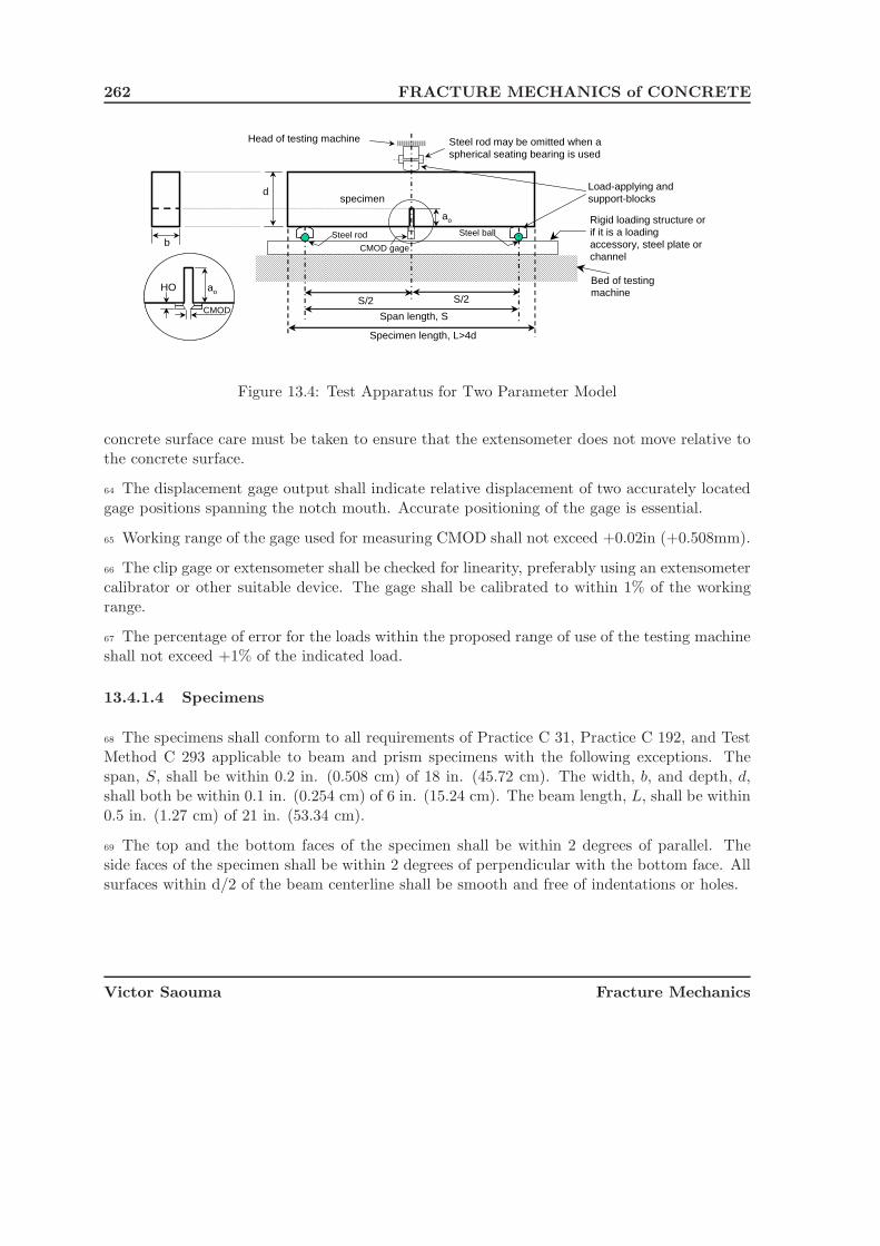
262 FRACTURE MECHANICS of CONCRETE
Bed of testing machine
Rigid loading structure or if it is a loading accessory, steel plate or channel
Load-applying and support-blocks
Steel rod Steel ball
specimen
Head of testing machine Steel rod may be omitted when a spherical seating bearing is used
S/2 S/2
d
Specimen length, L>4d
ao
Span length, S
bCMOD gage
CMOD
aoHO
CMOD
aoHO
Figure 13.4: Test Apparatus for Two Parameter Model
concrete surface care must be taken to ensure that the extensometer does not move relative tothe concrete surface.
64 The displacement gage output shall indicate relative displacement of two accurately locatedgage positions spanning the notch mouth. Accurate positioning of the gage is essential.
65 Working range of the gage used for measuring CMOD shall not exceed +0.02in (+0.508mm).
66 The clip gage or extensometer shall be checked for linearity, preferably using an extensometercalibrator or other suitable device. The gage shall be calibrated to within 1% of the workingrange.
67 The percentage of error for the loads within the proposed range of use of the testing machineshall not exceed +1% of the indicated load.
13.4.1.4 Specimens
68 The specimens shall conform to all requirements of Practice C 31, Practice C 192, and TestMethod C 293 applicable to beam and prism specimens with the following exceptions. Thespan, S, shall be within 0.2 in. (0.508 cm) of 18 in. (45.72 cm). The width, b, and depth, d,shall both be within 0.1 in. (0.254 cm) of 6 in. (15.24 cm). The beam length, L, shall be within0.5 in. (1.27 cm) of 21 in. (53.34 cm).
69 The top and the bottom faces of the specimen shall be within 2 degrees of parallel. Theside faces of the specimen shall be within 2 degrees of perpendicular with the bottom face. Allsurfaces within d/2 of the beam centerline shall be smooth and free of indentations or holes.
Victor Saouma Fracture Mechanics

13.4 Proposed ACI/ASCE Test Methods 263
13.4.1.5 Procedure
70 Fracture tests of moist cured specimens shall be made as soon as practical after removal frommoist storage. A notch shall be introduced within 0.25 in. (6.35 mm) of the mid-length of thebeam using a band saw or diamond tipped saw such that the width of the cut is no wider than3 mm. The notch shall be introduced as soon as possible prior to testing. The specimen shallbe kept moist at all times and shall be protected from moisture loss by wrapping it in a plasticor wet burlap sheet at the time of test.
71 The notch shall be cut within one degree of perpendicular to the longitudinal axis of thespecimen. The notch depth, ao, shall satisfy the inequality 0.25d < ao < 0.33d.
72 The length of the notch, ao, shall be measured from the bottom of the beam, on both faces,using a ruler with an accuracy of 0.5 mm. Each measurement shall be made three times oneach face. The measured notch depth on each side shall not differ by more than 5 percent. Thenotch length shall equal the average of the six measurements.
13.4.1.6 Specimen Testing
73 The specimen shall be placed in a testing machine in a center-point loading configuration asshown in Fig. 13.4. Use a closed-loop test machine with CMOD as the feedback. Continuouslymonitor both CMOD and the applied load, P , during the test.
74 Apply load using a constant rate of increment of CMOD such that the peak load, Pmax, isreached in between 1 and 10 minutes.
75 When the load has passed the maximum load and decreased to no more than 95% of thepeak load, reduce the applied load to between 1% and 5% of the peak load. Unloading can beperformed in CMOD or load control, and shall be accomplished in no less than 1 minute andno more than 10 minutes. Reload using the same loading rate until the load has passed themaximum load. A typical loading and unloading curve for concrete is shown in Fig. 13.5.
13.4.1.7 Measured Values
76 The following measured values shall be reported for each test: the dimensions L, S, b, andd; the mass, m0; and the initial notch length, a0. Report also the P-CMOD response of thespecimen, including the one cycle of loading and unloading in the post-peak.
13.4.1.8 Calculation
77 Calculation of fracture parameters, KIc(tp) and CTODc(tp), using the two-parameter fracturemethod (TPFM).
Victor Saouma Fracture Mechanics
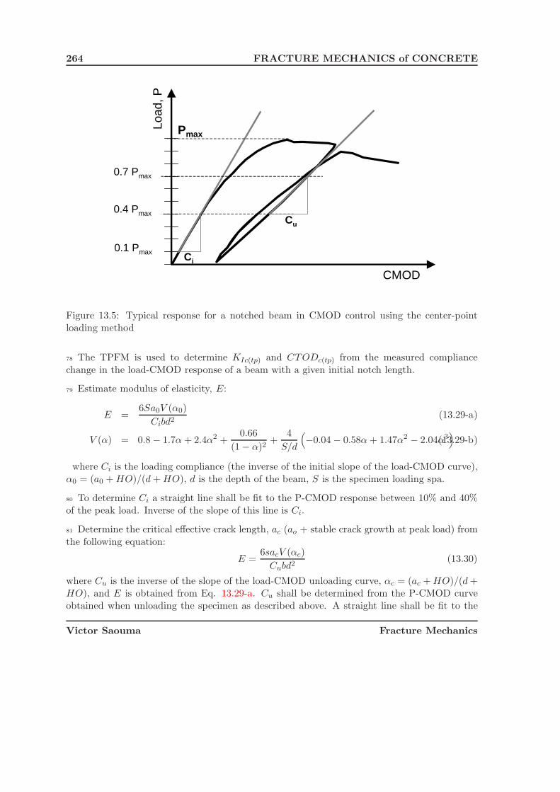
264 FRACTURE MECHANICS of CONCRETE
Load
, P
Cu
Ci
Pmax
0.4 Pmax
0.1 Pmax
0.7 Pmax
CMOD
Figure 13.5: Typical response for a notched beam in CMOD control using the center-pointloading method
78 The TPFM is used to determine KIc(tp) and CTODc(tp) from the measured compliancechange in the load-CMOD response of a beam with a given initial notch length.
79 Estimate modulus of elasticity, E:
E =6Sa0V (α0)
Cibd2(13.29-a)
V (α) = 0.8 − 1.7α + 2.4α2 +0.66
(1 − α)2+
4
S/d
(−0.04 − 0.58α + 1.47α2 − 2.04α3
)(13.29-b)
where Ci is the loading compliance (the inverse of the initial slope of the load-CMOD curve),α0 = (a0 + HO)/(d + HO), d is the depth of the beam, S is the specimen loading spa.
80 To determine Ci a straight line shall be fit to the P-CMOD response between 10% and 40%of the peak load. Inverse of the slope of this line is Ci.
81 Determine the critical effective crack length, ac (ao + stable crack growth at peak load) fromthe following equation:
E =6sacV (αc)
Cubd2(13.30)
where Cu is the inverse of the slope of the load-CMOD unloading curve, αc = (ac + HO)/(d +HO), and E is obtained from Eq. 13.29-a. Cu shall be determined from the P-CMOD curveobtained when unloading the specimen as described above. A straight line shall be fit to the
Victor Saouma Fracture Mechanics

13.4 Proposed ACI/ASCE Test Methods 265
unloading P-CMOD curve between 70% and 40% of the maximum load, Pmax. Inverse of theslope of this line is Cu.
82 Calculate the critical stress intensity factor index, KIc(tp):
KIc(tp) = 3(Pmax + 0.5W )S√
πacF (α)
2bd2(13.31-a)
F (α) =f1(α) + 4
S/d (f2(α) − f1(α)√
π(1 + 3α)(1 − α)3/2(13.31-b)
f1(α) = 1.99 + 0.83α − 0.31α2 + 0.14α3 (13.31-c)
f2(α) = 1.9 + 0.41α + 0.51α2 − 0.17α3 (13.31-d)
where Pmax is the maximum load, α = ac/d.
83 Calculate the critical crack tip opening displacement index, CTODc(tp):
CTODc(tp) =6PmaxSacV (α)
Ebd2
[(1 − β)2 + (1.081 − 1.149α)(β − β2)
]1/2(13.32-a)
V (α) = 0.76 − 2.28α + 3.87α2 − 2.04α3 +0.66
(1 − α)2(13.32-b)
where α = ac/d, and β = ao/ac.
13.4.2 Test 2: Cohesive Crack Model Parameters; Level 1 (Gf)
84 This standard provides a quantitative test method for determining fracture parameters ofhardened concrete. It assumes that the essential aspects of fracture of concrete can be describedby a cohesive or fictitious crack model, which is completely described by the cohesive stressversus crack opening curve, (Hillerborg, A. 1985). This method covers the determination ofthe initial linear portion of this curve for concrete using a combination of simple tests whichrequire measuring peak loads only. The determination of a bilinear approximation of the fullcohesive stress versus crack opening curve will be covered in a different standard.
85 This standard covers only mortars an concrete with maximum aggregate size of up to 25mm.
86 The values stated in SI units are to be regarded as the standard.
13.4.2.1 Terminology
13.4.2.1.1 Definitions
Stress versus crack opening curve or softening curve the relationship between the stress(σ) transferred between the faces of a cohesive crack and the crack opening (w), Fig. 13.6.
Victor Saouma Fracture Mechanics
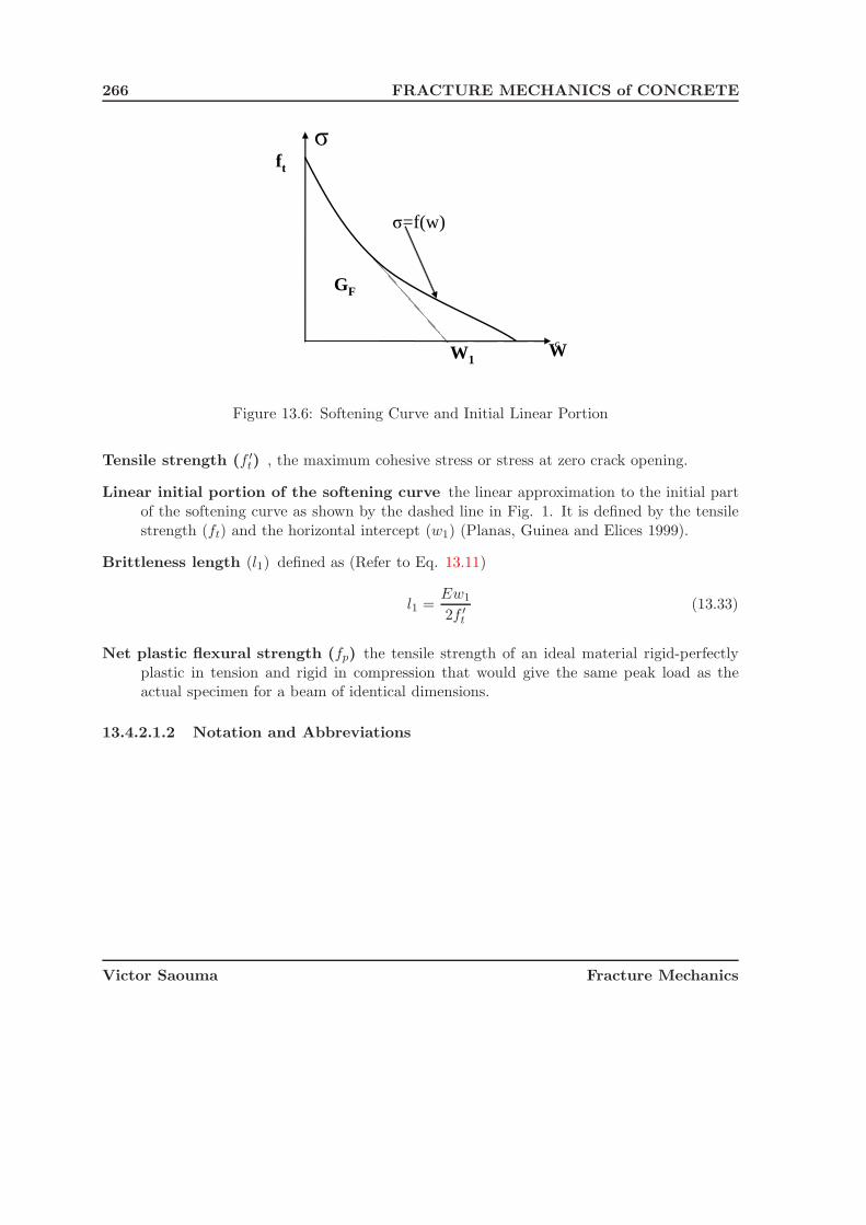
266 FRACTURE MECHANICS of CONCRETE
σ
WW1
ft
GF
σ=f(w)
c
Figure 13.6: Softening Curve and Initial Linear Portion
Tensile strength (f ′t) , the maximum cohesive stress or stress at zero crack opening.
Linear initial portion of the softening curve the linear approximation to the initial partof the softening curve as shown by the dashed line in Fig. 1. It is defined by the tensilestrength (ft) and the horizontal intercept (w1) (Planas, Guinea and Elices 1999).
Brittleness length (l1) defined as (Refer to Eq. 13.11)
l1 =Ew1
2f ′t
(13.33)
Net plastic flexural strength (fp) the tensile strength of an ideal material rigid-perfectlyplastic in tension and rigid in compression that would give the same peak load as theactual specimen for a beam of identical dimensions.
13.4.2.1.2 Notation and Abbreviations
Victor Saouma Fracture Mechanics

13.4 Proposed ACI/ASCE Test Methods 267
a0 notch length (initial crack length)b ligament length = D − a0
B thickness of specimenda maximum aggregate sizeD depth of specimenE elastic modulusEm mean elastic modulusf ′
t tensile strengthfp net plastic flexural strengthg specific gravity = 9.81 m s−2
l1 brittleness lengthL length of specimenm mass of the specimenN notch widthPmax corrected peak load of a specimenP ′
max measured peak load of a specimenS test span of the specimenT splitting tensile strengthTm mean splitting tensile strengthw cohesive crack openingw1 horizontal intercept of the linear initial portion of the softening curveα0 relative notch length
13.4.2.2 Summary of Test Method
87 In this test method, notched beams and cylindrical concrete specimens are tested to deter-mine fracture parameters of concrete.
88 The cohesive tensile strength (f ′t) is approximated by the splitting tensile strength of cylin-
drical concrete specimens tested according 496 (2000) (so-called Brazilian Test, as illustratedin Fig. 13.7), with minor modifications.
89 Center-point loading tests are run up to peak load on notched concrete beams and the netplastic flexural strength (fp) is determined from the peak load.
90 From the results of tensile strength (ft) and net plastic flexural strength (fp), the brittlenesslength (l1) is determined.
91 The elastic modulus (E) is determined according to ASTM C 469 test method.
92 The horizontal intercept (w1) is determined from the brittleness length (l1), the elastic mod-ulus (E) and the tensile strength (f ′
t) solving from Eq. 13.33.
Victor Saouma Fracture Mechanics

268 FRACTURE MECHANICS of CONCRETE
Figure 13.7: “Brazilian Test, (?)”
Victor Saouma Fracture Mechanics

13.4 Proposed ACI/ASCE Test Methods 269
13.4.2.3 Significance and Use
93 This test method is used to determine the initial linear portion of the softening curve for thecohesive crack model.
94 The cohesive crack model describes in a simplified manner the cracking of concrete keepinga good balance between accuracy and complexity.
95 Knowledge of only the linear initial portion of the softening curve is enough to solve somepractical problems such as the determination of structural peak loads (Planas et al. 1999) orthe description of the initial stages of cracking.
96 Care must be exercised in the interpretation and use of the material properties obtained bythis test method, because they are sensitive to any of the factors affecting concrete behaviorsuch as batching and mixing procedures, the methods of sampling, molding and fabrication andthe age, and temperature and moisture conditions during curing.
13.4.2.4 Specimens
97 Cylindrical specimens shall be used to determine the splitting tensile strength and the staticelastic modulus. The geometry and manufacture of these specimens shall conform to the generalprovisions of Practices C 31(field specimens) or C 192 (laboratory specimens).
98 Cylindrical specimens for splitting tensile strength shall further conform to any special pro-visions in Test Method C 496.
99 Cylindrical specimens for static elastic modulus shall further conform to any special provi-sions in Test Method C 469.
100 Beam specimens shall be used to determine the net plastic flexural strength. The geometryand manufacture of these specimens shall conform to the general provisions of Practices C 31(field specimens) or C 192 (laboratory specimens) applicable to beam and prism specimens.
101 A minimum of six cylindrical specimens and three beam specimens shall be cast. Wheneverpractical, all the specimens must be cast from the same concrete batch. If this is not possible,a number of cylinder specimens twice the number of beam specimens must be obtained fromeach batch. A minimum of three split cylinders, three cylinders for elastic modulus and threebeams must be tested.
102 The beam specimens shall be prismatic beams of rectangular cross section with a sawncentral notch Fig. 13.8. The beams defined in this standard are not to be used for materialswith a maximum aggregate size da larger than 25 mm.
1. The beam thickness (B) must be 150 ± 5 mm.
2. The beam depth (D) must be 150 ± 5 mm.
Victor Saouma Fracture Mechanics

270 FRACTURE MECHANICS of CONCRETE
Figure 13.8: Specimen Geometry and Dimensions
3. The loading span (S) must be equal to three times the beam depth (3D), within ±5 mm.
4. The total length (L) of the specimen shall be 50 mm longer than three times the beamdepth (3D + 50 mm) within ±5 mm.
5. The nominal notch depth (a0) shall be equal D/3. Deviations up to 10% of the nominalvalue may be accepted for a whole test series (0.30 ≤ a0/D ≤ 0.37). But, within a series,notch depths of individual specimens must not deviate from the mean more than 2%.
6. The notch width (N) must be no larger than 3 mm.
13.4.2.5 Casting, Curing and Conservation
103 After demolding, cure and conserve the specimens in a lime saturated bath at 23 ±2o Cuntil testing time.
104 After the removal of the specimen from the bath, and until the end of the test, drying ofthe surface of the specimen must be prevented.
13.4.2.6 Procedure
105 The procedure for splitting tensile tests shall be as described in the Test Method C 496,except that the loading rate shall be within the range 500 to 1000 kPa/min all the way up tothe peak load. Provisions shall be taken for measuring and recording the loading rate up to thepeak.
106 The procedure for static elastic modulus tests shall be as described in the Test Method C469.
107 Beam Specimen Preparation: The preparation of the beam specimens for testing may includegrinding of the load bearing areas, and notching.
Victor Saouma Fracture Mechanics

13.4 Proposed ACI/ASCE Test Methods 271
108 Gently place the specimen on the loading device. At this stage the rolling supports maybe clamped to ease the placement. Carefully center the specimen so that the notch is at midposition between the supports within 1 mm, and the mid-vertical-longitudinal plane of thespecimen coincides with the loading plane defined by the shafts b and h in Fig. 13.9 (within 1mm). An external frame with centering screws may prove useful to facilitate this task.
Figure 13.9: Sketch of a Loading Apparatus
109 Verify that the load channel is zeroed, and slowly pre-load the specimen up to a load ofbetween 5 and 10 % of the estimated maximum load. After the test, this pre-load must bechecked not to have exceed 15% of the actual peak load. If this limit had been exceeded, thetest must be considered invalid. During the pre-load, the spherical or cylindrical seatings mustbe free (and even helped) to accommodate any initial geometrical misfit.
110 Unclamp the rollers and run the test at constant crosshead rate. The rate must be selectedso that the peak load is reached within 3 to 5 min.
111 The test can be stopped after peak load is reached.
13.4.2.7 Calculations
13.4.2.7.1 Tensile strength, f ′t 112 Calculate the splitting tensile strength (T ) of each
cylinder specimen according to ASTM C 496, in SI units (kPa).
113 Determine the mean splitting tensile strength (Tm) by averaging over all the specimens.
114 Determine the tensile strength of concrete (for the cohesive crack model) as
ft =Tm
1000(13.34)
where Tm = mean splitting tensile strength, kPa, f ′t = tensile strength, MPa.
Victor Saouma Fracture Mechanics
272 FRACTURE MECHANICS of CONCRETE
13.4.2.7.2 Elastic modulus, E 115 Calculate the modulus of elasticity (E) of each cylinderspecimen according to ASTM C 469, in SI units (MPa).
116 Determine the mean elastic modulus (Em) by averaging over all the specimens.
13.4.2.7.3 Net plastic flexural strength, fp 117 Calculate the net plastic flexural strengthof each notched beam according to the following procedure:
1. From the test record or machine memory, determine the maximum load P ′max measured
by the load cell.
2. Determine the self-weight equivalent load P0 as
P0 = mg
(1 − L
2S
)(13.35)
where P0 = self-weight equivalent load, N. m = specimen mass, kg. g = specific gravity= 9.80 m s−2, L = specimen length, mm. S = loading span, mm.
3. Determine the maximum load corrected to take into account the weight of the specimenas
Pmax = P ′max + P0 (13.36)
where Pmax = corrected peak load, N; P ′max= measured peak load, N; P0 = self-weight
equivalent load, N.
4. Determine the net plastic flexural strength of the beam as:
fp =PmaxS
2Bb2(13.37)
where fp = net plastic flexural strength, MPa; Pmax = corrected peak load, N; B = beamthickness, mm; b = D − a0 = beam ligament, mm; D = depth of specimen, mm; a0 =notch length, mm; S = loading span, mm.
13.4.2.7.4 Brittleness length, l1, and horizontal intercept, w1 118 For each specimen,determine the brittleness length l1
l1 = κD
[11.2
(x2 − 1)2+
2.365
x2
](13.38)
where l1 = brittleness length, mm; κ = 1−α1.70 ; α0 = a0/D = notch-to-depth ratio; D = beam
depth, mm; a0 = notch length, mm; x = ft/fp; fp = net plastic flexural strength, MPa; ft =tensile strength, MPa.
119 Determine the average brittleness length l1m as the mean of the determinations for individ-ual specimens.
Victor Saouma Fracture Mechanics

13.4 Proposed ACI/ASCE Test Methods 273
120 Determine the horizontal intercept of the softening curve (w1) as
w1 = 10002ft
Eml1m (13.39)
where w1 = horizontal intercept, m (microns); ft = tensile strength, MPa; Em = mean elasticmodulus, MPa; l1m = brittleness length, mm.
13.4.3 Test 3: Cohesive Crack Model Parameters; Level 2 (GF )
121 This standard provides a quantitative test method for determining fracture parameters ofhardened concrete. It assumes that the essential aspects of fracture of concrete can be describedby a cohesive or fictitious crack model, which is completely described by the cohesive stressversus crack opening curve (Hillerborg, A. 1985).
122 This method covers the determination of a bilinear approximation of this curve for concreteusing a combination of split cylinder tests and bending tests on notched beams.
123 This standard covers only mortars an concrete with maximum aggregate size of up to 25mm.
124 The values stated in SI units are to be regarded as the standard.
13.4.3.1 Terminology
13.4.3.1.1 Definitions
Stress versus crack opening curve or softening curve: the relationship between the stress(σ) transferred between the faces of a cohesive crack and the crack opening (w), Fig. 13.10.
Tensile strength (ft), the maximum cohesive stress or stress at zero crack opening
Linear initial portion of the softening curve the linear approximation to the initial partof the softening curve as shown by the dashed line in Fig. 1. It is defined by the tensilestrength (ft) and the horizontal intercept (w1).
Brittleness length (l1) , defined as
l1 =Ew1
2ft(13.40)
Bilinear approximation of the softening curve a bilinear function that approximates theactual softening curve of concrete by a bilinear curve as shown in Fig. 13.11. The bilinearcurve is defined by 4 parameters, usually taken to be the tensile strength (ft), the criticalcrack opening (wc), and the crack opening and cohesive stress at the kink point (wk, σk).
Net plastic flexural strength (fp), the tensile strength of an ideal material rigid-perfectlyplastic in tension and rigid in compression that would give the same peak load as theactual specimen for a beam of identical dimensions.
Victor Saouma Fracture Mechanics

274 FRACTURE MECHANICS of CONCRETE
σ
WW1
ft
GF
σ=f(w)
c
Figure 13.10: Softening Curve and Initial Linear Portion
Softening curve
Stress,
ft
w1
wK
wc
Bilinear approximationKσ
σ
Figure 13.11: Softening curve and bilinear approximation
Victor Saouma Fracture Mechanics
13.4 Proposed ACI/ASCE Test Methods 275
13.4.3.1.2 Notation and Abbreviations
Victor Saouma Fracture Mechanics
276 FRACTURE MECHANICS of CONCRETE
a0 notch length (initial crack length)A far tail constantb ligament length = D − a0
B thickness of specimenCi initial compliance of beam specimenCMOD crack mouth opening displacementda maximum aggregate sizeD depth of specimenE elastic modulusEm mean elastic modulusft tensile strengthfp net plastic flexural strengthg specific gravity = 9.81 ms−2
GF mean fracture energyGFm fracture energy, area below the softening curveh distance from the CMOD measuring line to the specimen surfaceK tail fitting parameterl1 brittleness lengthl1m mean brittleness lengthL length of specimenm mass of the specimenN notch widthP total load on specimenP1 corrected load on specimen = P ′ − P ′
R
P ′R residual measured load at the end of test
Pmax effective peak load of a specimenP1max corrected peak load of a specimen = P ′
max − P ′R
P ′max effective peak load of a specimen
r distance from the measuring line of the displacement extensometers to thecenter plane of the specimen
S test span of the specimenT splitting tensile strengthTm mean splitting tensile strengthw cohesive crack openingw1 horizontal intercept of the linear initial portion of the softening curvewc critical crack opening (crack opening at which the cohesive stress vanishes)wch characteristic crack openingwG center of gravity of the softening curve
Victor Saouma Fracture Mechanics
13.4 Proposed ACI/ASCE Test Methods 277
wGm mean center of gravity of the softening curvewk crack opening at the kink point of the bilinear approximationwMA CMOD at zero P1
wMR CMOD at the end of the testWF total work of fractureWFm measured work of fractureX auxiliary variable for far tail fittingx inverse relative plastic strength = ft/fp
Y auxiliary variable for far tail fittingα0 relative notch length = a0/Dδ load point displacementδA load point displacement at zero P1
δR load point displacement at the end of testδk cohesive stress at the kink point of the bilinear approximation
13.4.3.2 Summary of Test Method
125 In this test method, notched beams and cylindrical concrete specimens are tested to deter-mine fracture parameters of concrete. The bilinear approximation is derived by forcing it 1)to give same peak loads as the actual softening curve for both the splitting cylinders and thenotched beams, 2) to have same fracture energy as the actual softening curve, and 3) to havesame center of gravity position as the actual softening curve.
126 The cohesive tensile strength (ft) is approximated by the splitting tensile strength of cylin-drical concrete specimens tested according ASTM C496 standard, with minor modifications.
127 Center-point loading tests are run under closed loop CMOD control on notched concretebeams (with compensation for the self-weight), and the curves of load versus load-point dis-placement and of load versus CMOD are recorded.
128 The net plastic flexural strength (fp) is determined from the peak load.
129 From the results of tensile strength (ft) and net plastic flexural strength (fp), the brittlenesslength (l1) is determined.
130 The elastic modulus (E) is determined from the initial slope of the load-CMOD curve.
131 The horizontal intercept (w1) is determined from the mean brittleness length (l1m), themean elastic modulus (Em) and the tensile strength (ft) solving from Eq. 13.40.
132 The fracture energy (GF ) is determined from the area under the load versus load-pointdisplacement curve.
133 The center of gravity of the area below the softening curve (wG) is computed by curve fittingof the far end of the load vs. CMOD curve.
Victor Saouma Fracture Mechanics

278 FRACTURE MECHANICS of CONCRETE
134 The critical crack opening (wc) and the coordinates of the kink point (wk, σk) are finallycomputed from simple geometrical relations from the set of values (ft, w1, GF , wg).
13.4.3.3 Significance and Use
135 This test method is used to determine a bilinear approximation of the softening curve forthe cohesive crack model.
136 The cohesive crack model describes in a simplified manner the cracking of concrete keepinga good balance between accuracy and complexity.
137 The actual softening curve of concrete can be approximated by a bilinear softening curveto get reasonable prediction of the overall cracking behavior, including peak load estimates,post-peak load-displacement response and energy dissipation.
138 Care must be exercised in the interpretation and use of the material properties obtained bythis test method, because they are sensitive to any of the factors affecting concrete behaviorsuch as batching and mixing procedures, the methods of sampling, molding and fabrication andthe age, temperature and moisture conditions during curing.
13.4.3.4 Specimens
139 Cylindrical specimens shall be used to determine the splitting tensile strength. The geometryand manufacture of these specimens shall conform to the general provisions of Practices C 31(field specimens) or C 192 (laboratory specimens).
140 Cylindrical specimens for splitting tensile strength shall further conform to any specialprovisions in Test Method C 496.
141 Beam specimens shall be used to determine the load vs. load-point displacement curve andthe load vs. CMOD curve. The geometry and manufacture of these specimens shall conformto the general provisions of Practices C 31(field specimens) or C 192 (laboratory specimens)applicable to beam and prism specimens.
142 A minimum of three cylindrical specimens and three beam specimens shall be cast. When-ever practical, all the specimens must be cast from the same concrete batch. If this is notpossible, a number of cylinder specimens twice the number of beam specimens must be ob-tained from each batch. A minimum of three split cylinders and three beams must be tested.
143 The beam specimens shall be prismatic beams of rectangular cross section with a sawncentral notch, Fig. 13.12. The beams defined in this standard are not to be used for materialswith a maximum aggregate size da larger than 25 mm. The beam thickness (B) must be 150±5mm. The beam depth (D) must be 150 ± 5 mm. The loading span (S) must be equal to threetimes the beam depth (3D), within ± 5 mm. The total length (L) of the specimen shall be 50mm longer than three times the beam depth (3D +50 mm) within ±5 mm. The nominal notch
Victor Saouma Fracture Mechanics

13.4 Proposed ACI/ASCE Test Methods 279
Figure 13.12: Specimen Geometry and Dimensions
depth (a0) shall be equal D/3. Deviations up to 10% of the nominal value may be acceptedfor a whole test series (0.30 ≤ a0/D ≤ 0.37). But, within a series, notch depths of individualspecimens must not deviate from the mean more than 2%. The notch width (N) must be nolarger than 3 mm.
144 After demolding, cure and conserve the specimens in a lime saturated bath at 23±2oC untiltesting time.
145 After the removal of the specimen from the bath, and until the end of the test, drying ofthe surface of the specimen must be prevented.
13.4.3.5 Apparatus
146 Apparatus for splitting tensile strength shall conform to the provisions of Test Method C496, except that the bearing strips shall be 10 mm wide.
147 Servohydraulic or electromechanical testing machines, Fig. 13.3 shall be used that provideclosed-loop control with the crack mouth opening displacement (CMOD) as the feedback signal.High machine stiffness is recommended. In addition, the testing machine shall conform to therequirements of the Sections on Basis of Verification, Corrections, and Time Interval BetweenVerifications of Practices E 4.
148 The load cell installed on the machine for these specific tests must give load readings accuratewithin 1% of the recorded peak load.
149 The CMOD must be measured with a clip-on gage or similar extensometer giving readingsaccurate within 5 μm (five micron) over a range of 2 mm.
150 The gage length of the extensometer must be centered on the notch; The gage length mustbe less than 0.2D.
151 To avoid measuring the inelastic deformation originated at the supports, the displacement
Victor Saouma Fracture Mechanics

280 FRACTURE MECHANICS of CONCRETE
must be determined relative to the points directly above and below the loading points by meansof a reference frame.
152 For this method to give accurate results, the frame for measuring the displacement shallbe stiff enough. At the worse situation, a maximum frame deflection of 2 μm (two microns) isallowed. The frame must stay on two ground hardened steel plates at the vertical of the lateralsupports.
153 Two extensometers shall be symmetrically placed at both sides of the notch, at the bottomface of the specimen. The distance (r) from the measuring line to the center plane of thespecimen shall be as small as possible. The load point displacement signal (δ) shall be computedas the average of the measuring signal of both extensometers.
154 The extensometers shall give readings accurate within 10 μm (ten microns) over a range of5 mm.
155 The loading apparatus for the bending tests will provide two supports and a central loadingblock suitably mounted to minimize eccentricities (torsion), to keep the loading span withinthe specified tolerances, and to minimize friction at the supports.
156 Weight compensation by using specimens longer than twice the loading span (L = 2S + 50mm) is very effective, although the weight of the specimen is very much increased and handlingmore difficult.
13.4.3.6 Test Record
157 Record of the load-CMOD curve must be performed so that there is no loss of resolution.
158 The time-delay between readings must be selected in such a way as to comply the followingconditions: (1) a minimum of 20 well spaced readings must be performed in the load intervalspanning from 0.15 to 0.55 of the final peak load; (2) the reading interval in the peak zoneof the test must be low enough for the three load readings immediately before and after thepeak be within 1% of the peak; (3) at least 20 well spaced readings must be recorded in thepost peak region when the load decreases from the peak to 0.15 of the peak, (4) a minimumof 150 well spaced readings must be recorded in the post peak region up to the end of the test(conventionally considered to occur when the CMOD reaches 2 mm).
13.4.3.7 Procedure
159 The procedure for splitting tensile tests shall be as described in the Test Method C 496,except that the loading rate shall be within the range 500 to 1000 kPa/min all the way up tothe peak load. Provisions shall be taken for measuring and recording the loading rate up to thepeak.
Victor Saouma Fracture Mechanics

13.4 Proposed ACI/ASCE Test Methods 281
160 The preparation of the specimen for testing may include grinding of the load bearing areas,preparation of attachment for clip-on gage, and notching.
1. Immediately after removing the specimen from the bath, mark the central section andthe loading lines of the lateral supports (use pencil, not scaring instruments). Protectthe surface to avoid drying, by coatings, wet clothes and water-spraying so that drying iscompletely avoided.
2. Verify that the load-bearing areas and the contact zones with the vertical extensometersare plane using a ground steel rod and leaf-type feeler gages of 0.1 mm. If any gaps largerthan 0.1 mm are detected, grind the surface of the specimen to eliminate the gap.
3. Drill any hole that may be required to fasten the knife edges for the clip gage. Gluing ofknife edges on the moist surface is not recommended.
4. Cut the notch so that the notch front is perpendicular to planes that were horizontalduring casting. Use a diamond saw with water refrigeration and keep the load as smallas possible to avoid damaging the concrete.
5. Handling of the specimen after notching must be very gentle to avoid damage. Lifting ofthe specimen must be performed by means of two attachments located at 1/4 from theends of the specimens. Shocks must be avoided at all times.
6. Attach the elements to hold the clip-on gage.
7. Attach the hardened steel plates at the locations of the rolling supports.
161 Beam Test:
1. Gently place the specimen on the loading device. At this stage the rolling supports maybe clamped to ease the placement. Attach the clip-on gage and set its output to zero(or record the initial reading). Carefully center the specimen so that the notch is at midposition between the supports within 1 mm or 0.25% of the span (whichever is the less),and the mid-vertical-longitudinal plane of the specimen coincides with the loading planedefined by the shafts b and h (within 0.5 mm or 0.5 % of the beam thickness). An externalframe with centering screws may prove useful to facilitate this task.
162 Place the hardened steel plates at the vertical of the lateral supports and the referenceframe and the transducers for measuring the load point displacement, and set its outputto zero (or record the initial reading). The supports of the frame must be placed onthe vertical of the lateral supports of the specimen within 1 mm or 0.25% of the span(whichever is the less).
2. Verify that the load channel is zeroed, and slowly pre-load the specimen up to a load ofbetween 5 and 10% of the estimated maximum load. After the test, this pre-load must be
Victor Saouma Fracture Mechanics

282 FRACTURE MECHANICS of CONCRETE
checked not to have exceeded 15% of the actual peak load. If this limit was exceeded, thetest must be considered invalid. During the pre-load, the spherical or cylindrical seatingsmust be free (and even helped) to accommodate any initial geometrical misfit.
3. Unclamp the rollers and run the test under at constant CMOD rate. The rate must beselected so that the peak load is reached within 3 to 5 min. 8.4. Specimen Dimensions:
4. Measure the dimensions of the cross section to the nearest 0.1 mm. Measure the beamdepth (D) at the central cross section at the two surfaces of each half of the specimen,and take the mean of the four measurements. Measure the notch depth (a0) at the centralcross section at the two surfaces of each half of the specimen and take the mean of thefour measurements. Measure the beam thickness (B) at the front of the notch and atthe top of the beam for the two halves of the specimen and take the mean of the fourmeasurements.
13.4.3.8 Calculations
13.4.3.8.1 Tensile strength, ft 162 Calculate the splitting tensile strength (T ) of eachcylinder specimen according to point 7.1 of ASTM C 496, in SI units (kPa).
163 Determine the mean splitting tensile strength (Tm) by averaging over all the specimens.
164 Determine the tensile strength of concrete (for the cohesive crack model) as
ft =Tm
1000(13.41)
where Tm = mean splitting tensile strength, kPa; ft = tensile strength, MPa.
13.4.3.8.2 Elastic modulus, E 165 Calculate the elastic modulus of each notched beamaccording the following procedure:
1. From the load-CMOD record, select a linear segment with measured loads between 15%and 55% of the peak load (0.15P ′
max ≤ P ′ ≤ 0.55P ′max).
2. Fit a straight line to this segment with all the data available. Use linear regression ofCMOD vs. P . to determine the slope of the segment, which is taken to coincide with theinitial compliance of the specimen:
Ci =Δ(CMOD)
ΔP ′ (13.42)
where Ci = initial compliance, μm N−1; Δ(CMOD) = variation of CMOD, μm; P ′ =variation of measured load, N;
Victor Saouma Fracture Mechanics

13.4 Proposed ACI/ASCE Test Methods 283
3. Determine the elastic modulus as
E =24
CiBD[a0V1(α0) + hW1(α0)] (13.43)
where E = elastic modulus, GPa; Ci = initial compliance, μm N−1; B = beam thickness,mm; D= beam depth, mm; a0 = notch length, mm; α0 = relative notch length = a0/D;h = Distance of the knife edges to specimen surface, mm; and
V1(α) = 0.76 − 2.28α0 + 3.87α20 − 2.04α3
0 +0.66
(1 − α0)2(13.44-a)
W1(α) = 20.184 − 82.790α0 + 121.64α20 (13.44-b)
4. Determine the mean elastic modulus (Em) by averaging over all the specimens.
13.4.3.8.3 Far tail constant, A 166 Determine the residual load P ′R measured by the load
cell at the end of the test, for CMOD = 2 mm or nearest point on the record. Determine thecorresponding CMOD (wMR). Delete the recorded points with CMOD larger than wMR.
167 Compute, for all the record points, the corrected load P1 by subtracting from the measuredload the residual load: P1 = P ′ − P ′
R
168 Plot the curve of corrected load P1 versus CMOD. Determine the value wMA of the inter-section of the rising part of the curve with the CMOD axis (Fig. 13.13).
Figure 13.13: Plot of corrected load P1 versus CMOD.
169 For the points in the record past the peak for which the corrected load is less than or equalto 5% of the corrected peak load, compute the quantity X defined as
X =1
(wM − wMA)2− 1
(wMR − wMA)2(13.45)
Victor Saouma Fracture Mechanics

284 FRACTURE MECHANICS of CONCRETE
where wM = recorded CMOD, mm; wMR = CMOD at the end of test, mm; wMA = CMOD atzero P1 for the rising part of curve, mm.
170 Plot P1 versus x and perform a least-squares fit of the quadratic equation
P1 = X(A + KX) (13.46)
Find A and K by least-squares fitting and give A in N mm2 with three significant digits (K isnot needeed).
NOTE. Most computer packages for curve plotting will be able to perform the foregoingnonlinear fit. However, if such a program is not available, a linear regression of Y = P1/Xversus X will solve the problem.
13.4.3.9 Net plastic flexural strength, fp
171 Calculate the net plastic flexural strength of each notched beam according to the followingprocedure:
1. Determine the effective peak load taking into account the finite length of the tail of therecord as
Pmax = P1max +A
(wMR − wMA)2(13.47)
where Pmax = effective peak load, N; P1max = corrected peak load, N. A = far tailconstant, Nmm2; wMR = CMOD at the end of test, mm; wMA = CMOD at zero P1 forthe raising part of curve, mm;
2. Determine the net plastic flexural strength of the beam as:
fp =PmaxS
2Bd2(13.48)
where fp = net plastic flexural strength, MPa; Pmax = effective peak load, N; B = beamthickness, mm; b = D − a0 = ligament length, mm; D = depth of specimen, mm; a0 =notch length, mm; S = test span of the specimen, mm.
13.4.3.10 Brittleness length, l1, and horizontal intercept, w1
172 For each specimen, determine the brittleness length l1
l1 = κD
[11.2
(x2 − 1)2+
2.365
x2
](13.49)
where l1 = brittleness length, mm; κ = 1−α1.70 ; α0 = a0/D = notch-to-depth ratio; D = beam
depth, mm; a0 = notch length, mm; x = ft/fp = inverse relative plastic strength; fp = netplastic flexural strength, MPa; ft = tensile strength, MPa.
Victor Saouma Fracture Mechanics

13.4 Proposed ACI/ASCE Test Methods 285
173 Determine the mean brittleness length l1m as the average of the determinations for individualspecimens.
174 Determine the horizontal intercept of the softening curve (w1) as
w1 = 10002ft
Eml1m (13.50)
where w1 = horizontal intercept, μm (microns); ft = tensile strength, MPa; Em = mean elasticmodulus, MPa; l1m = mean brittleness length, mm.
13.4.3.11 Fracture energy GF
175 For each specimen, plot the curve of corrected load P1 versus load-point displacement δ.Determine the value δA of the intersection of the raising part of the curve with the δ-axis, Fig.13.14.
176 For each specimen, determine the load-point displacement δR of the last point of the testrecord
For each specimen, compute the measured work of fracture WFm as the area enclosedbetween the positive part of the P1 vs. δ curve and the δ axis. Express it in N mm (mJ) to thenearest 5 N mm.
177 For each specimen, compute the total work of fracture WF as
WF = WFm +2A
δR − δA(13.51)
where WF = total work of fracture, N mm (mJ); WFm = measured work of fracture, N mm(mJ); A = far tail constant N mm2; δR = load-point at the end of test, mm; δA = CMOD atzero P1 for the raising part of curve, mm.
178 For each specimen, compute the fracture energy GF as
GF = 1000WF
Bb(13.52)
where GF = fracture energy, N/m (J/m2); WF = total work of fracture, N mm (mJ); B =beam thickness, mm; b = D − a0 = ligament length, mm.
179 Determine the mean fracture energy GFm as the average of the determinations for individualspecimens.
13.4.3.12 Center of gravity of the softening curve, wG
180 For each specimen, compute the abscissa of the center of gravity of the area under thesoftening curve as
wG =4A
BSGF× 10−6 (13.53)
Victor Saouma Fracture Mechanics

286 FRACTURE MECHANICS of CONCRETE
Figure 13.14: Plot of corrected load P1 versus load-point displacement δ
where wG =center of gravity of the area under the softening curve, μm (microns); A = far tailconstant, N mm2; B = beam thickness, mm; S = loading span, mm; GF = fracture energy ofthe specimen, N/m.
181 Determine the mean center of gravity wGm as the average of the determinations for individualspecimens.
13.4.3.13 Critical crack opening, wc
182 Compute the characteristic crack opening defined as
wch =GFm
ft(13.54)
where wch = characteristic crack opening, μm (microns); GFm = mean fracture energy, N/m;ft = tensile strength, MPa.
183 Compute the critical crack opening of the bilinear approximation as
wc = wch3wGm − w1
2wch − w1
[1 +
√1 − 2w1(3wGm − 2wch)(2wch − w1)
wch(3wGm−w1)2
](13.55)
where wc =critical crack opening, μm (microns); wch = characteristic crack opening, μm(microns); wGm = mean center of gravity of the area under the stress versus crack openingcurve, μm (microns) w1 = horizontal intercept, μm (microns).
13.4.3.14 Coordinates at the kink point (σk, wk)
184 Compute the stress at the kink point of the bilinear approximation as
σk = ft2wch − w1
wc − w1(13.56)
Victor Saouma Fracture Mechanics

13.5 Wedge Splitting Test; Saouma et. al. 287
where σk = stress at the kink point, MPa; ft = tensile strength, MPa; wch = characteristic crackopening, μm (microns); w1 = horizontal intercept, μm (microns); wc =critical crack opening,μm (microns).
185 Compute the crack opening at the kink point of the bilinear approximation as
wk = w1wc − 2wch
wc − w1(13.57)
where wk = crack opening at the kink point, μm (microns); wc = critical crack opening, μm(microns); wch = characteristic crack opening, μm (microns); w1 = horizontal intercept, μm(microns).
13.5 Wedge Splitting Test; Saouma et. al.
This paper proposes consideration of the wedge splitting test configuration to determine boththe fracture toughness and the fracture energy of rock.
The test method introduces, through a wedge, a controlled lateral opening displacement toinduce stable crack growth in a prismatic or cylindrical specimen, Fig. 13.15. From the splittingforce - average crack opening displacement response of the specimen, the specific fracture energyis determined. For fracture toughness evaluation, a series of unload-reload is necessary.
Figure 13.15: Principle of the Wedge Splitting Test Set-up
This test method provides a means of measuring rock’s resistance to crack propagationthrough linear elastic fracture mechanics (KIc) or nonlinear fracture mechanics (GF ). Resultsof this method may be used in numerical simulations as well as in comparative studies of thefracture properties of different rocks.
13.5.1 Apparatus
Testing System - The testing system consists of frame, actuator, force cell, controller, and data
Victor Saouma Fracture Mechanics

288 FRACTURE MECHANICS of CONCRETE
acquisition equipment as a minimum. Whereas it is preferable to have a closed-loop servo-controlled machine, this is not essential if the testing machine is rigid enough.
1. Force Cell - The force-measuring device shall have sufficient capacity and shall be accurateto within 1.0 % of the peak force measured in the test.
2. Displacement Measurement Devices - Two displacement measuring devices shall be usedfor measuring the displacements in the axis of the horizontal splitting force, one on eachside of the specimen (COD1 on side 1, COD2 on side 2). The displacement measurementdevices shall be of a type having sufficient capacity to enable the complete splitting ofthe specimen in two halves, and shall be accurate to within 1.0 % of the displacementmeasured while the specimen is at peak force.
Test Set-up - The principle of the wedge splitting test set-up, Fig. 13.15, with the successivesteps, from 1 to 3, of mounting of the test for a prismatic specimen. The test set-up betweenthe actuator or force cell and the specimen consists of a beam with wedges (A), plates equippedwith roller bearings (B), and a rounded support (C).
13.5.2 Test Specimens
Specimen Configuration and Dimensions - The wedge splitting test specimen can be eitherprismatic or cylindrical, cast in moulds or taken as cores from the structure. Dimensionsare shown below on Fig. 13.16 (all dimensions in mm). The following ligament lengths arerecommended to obtain a stable crack propagation and to avoid unintentional mixed modecrack propagation:Closed-loop control of COD: h1 = 130 mm.Stroke control: h1 = 85 mm.
It should be noted that these are recommended values for “stiff” rock. For “soft” rock(defined by a relatively low fracture energy GF ), it is recommended to use a ligamnet length of85 mm in conjunction with a closed-loop COD control.
Specimen Preparation - The groove and notch shall be cut into the specimen. In order toforce a straight path of the crack propagation, a 5 mm deep groove can be cut on both sides ofthe specimen, on the surface following the plane of the ligament.
13.5.3 Procedure
1. Place displacement measuring systems on both sides of the specimen.
2. Place specimen on a suitable rounded support.
3. Carefully insert the wedge between the roller bearings.
4. Bring the wedges in contact with the roller bearings and perform the test, in either oneof two test control modes:
Victor Saouma Fracture Mechanics
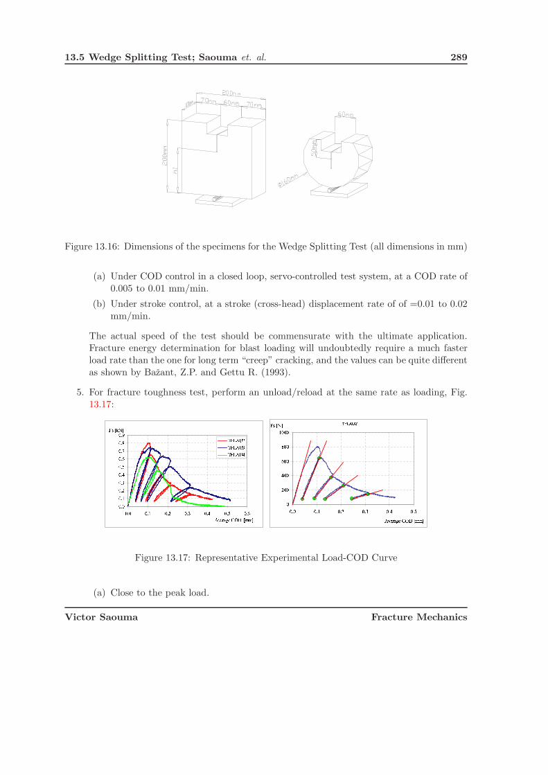
13.5 Wedge Splitting Test; Saouma et. al. 289
Figure 13.16: Dimensions of the specimens for the Wedge Splitting Test (all dimensions in mm)
(a) Under COD control in a closed loop, servo-controlled test system, at a COD rate of0.005 to 0.01 mm/min.
(b) Under stroke control, at a stroke (cross-head) displacement rate of of =0.01 to 0.02mm/min.
The actual speed of the test should be commensurate with the ultimate application.Fracture energy determination for blast loading will undoubtedly require a much fasterload rate than the one for long term “creep” cracking, and the values can be quite differentas shown by Bazant, Z.P. and Gettu R. (1993).
5. For fracture toughness test, perform an unload/reload at the same rate as loading, Fig.13.17:
Figure 13.17: Representative Experimental Load-COD Curve
(a) Close to the peak load.
Victor Saouma Fracture Mechanics

290 FRACTURE MECHANICS of CONCRETE
(b) At least 4 times in the post-peak zone.
Fig. 13.18 illustrates the test set-up with a (prismatic) specimen with the forces induced by theimposed COD or crosshead displacement. The resultant splitting force acts at 10 mm belowthe top side of the specimen.
Figure 13.18: Test set-up and acting forces, for a prismatic specimen
13.5.4 Measured Values
Measured values are: 1) Vertical force FV as a function of time; and 2)Crack Opening Displace-ments COD1 and COD2 on both sides of the specimen, as a function of time.
13.5.5 Calculation
13.5.5.1 Fracture Toughness
The determination of the fracture toughness requires not only the maximum load but also thecorresponding crack size. However, in rock, as in concrete, the tip of the crack may not beeasily identifiable due to the heterogeneity introduced by the fine grains. Hence, the conceptof an elastic equivalent crack length has to be used to determine the fracture toughness. Thisis determined through the compliance method which combines finite element calibration withanalysis of experimental data.
This Finite (or boundary) element analysis of the geometry, with E = 1, is conducted intwo parts. First a unit horizontal load is applied at the location of the wedges, and the initial
Victor Saouma Fracture Mechanics

13.5 Wedge Splitting Test; Saouma et. al. 291
normalized compliance is determined. In this case C0n is simply equal to the CODFS
measuredalong a unit splitting force FS .
186 Subsequently, geometries with increasing crack lengths (again with E = 1) are also subjectedto a unit FS and analyzed. For each analysis (crack length, a) we compute: the fracturetoughness, and the compliance. These analyses results are then tabulated, and a least squarebest fit is performed to determine aeff = aeff (Cn), and KIc = KIc(aeff ), where aeff is theeffective crack length.
187 Fig. 13.19, and 13.20 show representative normalized and actual compliance and stressintensity factor curves.
0
5
10
15
20
0 20 40 60 80
0,00
0,02
0,04
0,06
0,08
0 20 40 60 80
Figure 13.19: Normalized Compliance and Stress Intensity Factors in Terms of Crack Length a
0,0000
0,0005
0,0010
0,0015
0,0020
0,0025
0,0030
0 20 40 60 80
Cexp
0,0000
0,0005
0,0010
0,0015
0,0020
0,0025
0,0030
0 20 40 60 80
Cexp
0,00
0,02
0,04
0,06
0,08
0 20 40 60 800,00
0,02
0,04
0,06
0,08
0 20 40 60 80
Figure 13.20: Compliance and Stress Intensity Factors in Terms of Crack Length a
At this point, test interpretation proceeds as follows:
Victor Saouma Fracture Mechanics

292 FRACTURE MECHANICS of CONCRETE
1. From the first unload-reload cycle, determine the effective elastic modulus from
Eeff =C0
n
C0exp
(13.58)
Where C0n is the normalized compliance (obtained from the pre-test calibration) and C0
exp
is the initial experimental compliance given by
C0exp =
CODFS
FS(13.59)
where CODFSis the crack mouth opening displacement measured along the splitting
force FS .
2. Having determined the effective elastic modulus, the normalized compliance is determinedfrom Cn = EeffCexp.
3. For each of the subsequent post-peak response determine:
(a) The experimental compliance, Cexp.
(b) The corresponding elastic equivalent (or effective) crack length from
aeff = aeff (Cn) (13.60)
(c) The fracture toughness for this particular crack length
KIc = KIc(aeff ) (13.61)
4. Plot the determine fracture toughnesses in terms of effective crack length, and determinethe average value. It should be noted that as aeff approaches the ligament length (distancefrom tip of the notch to the bottom of the specimen), there will be a small decrease inKIc.
13.5.5.2 Fracture Energy
1. Determine the (horizontal) splitting force acting on the roller bearing, FS from:
FS =1
2 tan αFV =
1
2 tan 15oFV = 1.866FV (13.62)
2. Determine the average of the two displacements measured:
COD =COD1 + COD2
2(13.63)
3. Plot FS in terms of average COD and, if necessary, extrapolate curve to zero FS .
Victor Saouma Fracture Mechanics

13.5 Wedge Splitting Test; Saouma et. al. 293
Fs
Average COD
WF
GF = WF/Alig (J/m2)
Figure 13.21: Definition of the work of fracture and specific fracture energy
4. Determine the ligament area ALig corresponding to the projected area of the crack on theligament.
5. Determine the work of fracture WF as the area under the FS −COD curve (Fig. 13.21).
6. Determine the specific fracture energy GF :
GF =WF
ALig(13.64)
13.5.6 Report
Report the following information:
1. Specimen dimensions
2. Test control method (stroke displacement or COD control, and displacement rate).
3. Description of the fracture surface, especially any unusual appearance or significant devi-ation from a vertical plane centered on the pre-notch tip.
4. Splitting force - average COD curve.
5. Work of Fracture WF and Specific Fracture Energy GF .
13.5.7 Observations
Major advantages of the proposed test include:
1. Can be run on usual mechanical testing machines in compression mode (albeit with alonger relative notch length), or on a servo-controlled one.
2. Can be performed on specimens, prismatic or cylindrical cores extracted from the rock.
Victor Saouma Fracture Mechanics

294 FRACTURE MECHANICS of CONCRETE
3. Has a substantially longer ligament length per unit weight of concrete as compared toother tests (and in particular compared to the Three-Point-Bending-Beam Test), and asmaller amount of elastic strain energy is stored in the specimen during cracking. Thisis a particularly important characteristic which facilitates stable tests without risks ofsnap-backs.
4. Self-weight effect can be neglected for usual sizes (20 x 20 x 10 cm prismatic specimen)(Denarie, E. and Saouma, V.E. and Iocco, A. and Varelas, D. 1999).
5. Test set-up and specimen geometry can be easily adapted for bigger or smaller specimensizes, (Trunk 2000).
6. Has been for now 15 years extensively used by researchers, and practitioners in the US,Europe and Japan with specimens ranging from 5 cm up to 3.2 m in size, on various typesof concretes, mortars, advanced cementitious materials and rock.
Moreover, the interpretation of the tests results for the determination of GF as well asthe tensile softening diagram is straightforward and requires only very simple calculations.In a first approximation, the derivation of the tensile softening diagram can be based on theregressions performed on extensive data sets, for different types of concretes, at quasi-staticimposed displacement rates, (Bruhwiler, E. 1992). The uniaxial tensile strength ft should bepreferably determined experimentally by means of a uniaxial tensile test. If adequate softwaremodules are available, ft and the tensile softening diagram can also be indirectly determined bymeans of an inverse analysis using a FEM simulation of the experimental specimen response,(Bolzon, Fedele and Maier 2002).
Finally, this test has been used by one of the author to test limestone, (Bruhwiler, E., andSaouma, V.E., 1990) and limestone concrete interfaces, (Chandra and Saouma 2004).
Victor Saouma Fracture Mechanics

Chapter 14
SIZE EFFECT
Paper in print
1 Crack bridging occurs when cohesive stresses join the opposite faces of a crack, shielding thetip from the full effect of the applied load and thus giving rise to increased fracture resistance.Cohesive stresses are present both in elasto-plastic materials such as metals (through cracktip yielding), (Dugdale 1960), (Barenblatt 1962) and in quasi-brittle ones. In the later, theyare present not only in cementitious materials, but also in ceramics, (Saouma, Natekar andSbaizero 2002) and are caused by reinforcing fibers, particles (such as aggregates or inclusions),or simply regions of microscopically irregular crack surfaces causing topological interference.
2 Cohesive stress models were first suggested by Dugdale (1960) using a constant stress, thenBarenblatt (1962) generalized this concept to a more general stress distribution, one whichcauses the crack faces to close smoothly. It should be noted that those two pioneering studiesattributed different causes to the cohesive stresses. For Dugdale it was caused by macroscopicplasticity (and can be of any size) while for Barenblatt it was caused by molecular cohesion (andmust be restricted to a relatively very small zone), (Kanninen and Popelar 1985). Finally, mostrecently Hillerborg, A. and Modeer, M. and Petersson, P.E. (1976a) assumed a nonlinear modelwhere the stress is a function of the crack opening. The first two models are most appropriatefor metals to account for the presence of a plastic zone, whereas Hillerborg’s model is moresuited for cementitious material with a fracture process zone.
3 In both Dugdale and Barenblatt solution, the stress intensity factors caused by the far fieldload, and the cohesive stresses are assumed to cancel each other. Hence, implicit in this as-sumption is a zero material fracture toughness.
4 Finally, Hillerborg does not consider any singularity at the tip of the crack. Implicit in hisapproach is that there can not be a stress singularity at the crack tip since the criterion for crackpropagation is based on the crack tip stress. This assumption was recently challenged by Xuand Reinhardt (1998) who developed the double-K criterion where KR(Δa) = Kini
Ic + KC(Δa)and KC(Δa) = F (ft, f(σ),Δa). In this model, developed for concrete, the resistance to crack

296 SIZE EFFECT
growth (right hand side) is first set to the inherent toughness, and then to a cohesive term.Hence, contrarily to Hillerborg’s model, a cohesive stress does not necessarily eliminate thestress singularity, and as such crack propagation is no longer governed by a stress criteria, butrather by a modified linear elastic fracture mechanics one. This model enables us to distinguishbetween initial crack growth (in the absence of a fracture process zone) governed by Kini
Ic andsubsequent unstable crack growth in terms of Kini
Ic + KC(Δa). Despite its appeal, this modelhas not yet been widely embraced by the concrete research community which continues to use(for the most part) Hillerborg’s model.
5 In this chapter, we shall closely examine the role played by the cohesive stresses in inducinga size effect. This has already been suggested by Karihaloo (1996) “... the origin of the sizeeffect is in the non-sigular stress distribution ahead of the notch/crack”.
6 Hence, keeping with the original spirit of the derivations of Dugdale, Barenblatt and Hillerborgwe will assume the (net) fracture toughness to be zero.
14.0.1 Original Derivation
7 Bazant, Z. and Planas, J. (1998) presented a unified model for the nominal strength of quasi-brittle material. This simple and elegant equation is asymptotic to plasticity and linear elasticfracture mechanics, while capturing the intermediary quasi-brittle response.
8 Considering the energy exchanged during an infinitesimal crack extension in a plate of widthD, Fig. 16.5, the energy released can be approximated by b2k(a0 + cf )Δaσ2
n/2E, which mustbe equal to the energy consumed during crack growth: bGF Δa, hence
b2k(a0 + cf )Δaσ2n/2E = bGF Δa (14.1)
yielding
σn =Bf ′
t√1 + D
D0
(14.2)
where
Bf ′t =
√GF E
kcfand
D
D0=
a0
cf= β (14.3)
9 In his original paper, Bazant, Z.P. (1984) noted that the analytical or numerical derivationof B and β is too difficult, and they are best obtained through statistical regression analysis oftest data.
10 This derivation would be characterized as semi-analytical, since it combines an analyticalderivation (albeit with some simplifying assumptions), and experimental derivation of constantstoo complicated to be derived analytically. Finally, this derivation does not explicitly referencea plasticity and/or a linear elastic fracture mechanics solution. Yet, those two solutions areultimately asymptotic to the derived size effect law.
Victor Saouma Fracture Mechanics
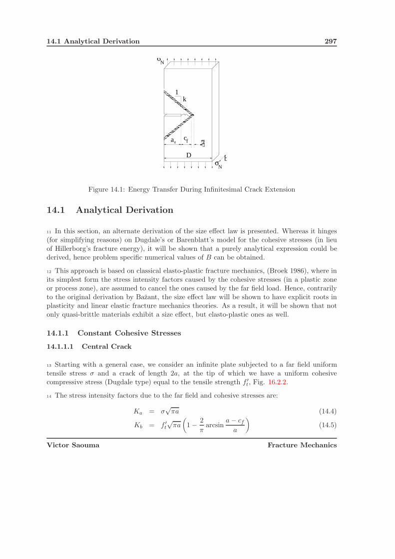
14.1 Analytical Derivation 297
σN
cf aΔ
Dσ
a
N
b
1k
0
Figure 14.1: Energy Transfer During Infinitesimal Crack Extension
14.1 Analytical Derivation
11 In this section, an alternate derivation of the size effect law is presented. Whereas it hinges(for simplifying reasons) on Dugdale’s or Barenblatt’s model for the cohesive stresses (in lieuof Hillerborg’s fracture energy), it will be shown that a purely analytical expression could bederived, hence problem specific numerical values of B can be obtained.
12 This approach is based on classical elasto-plastic fracture mechanics, (Broek 1986), where inits simplest form the stress intensity factors caused by the cohesive stresses (in a plastic zoneor process zone), are assumed to cancel the ones caused by the far field load. Hence, contrarilyto the original derivation by Bazant, the size effect law will be shown to have explicit roots inplasticity and linear elastic fracture mechanics theories. As a result, it will be shown that notonly quasi-brittle materials exhibit a size effect, but elasto-plastic ones as well.
14.1.1 Constant Cohesive Stresses
14.1.1.1 Central Crack
13 Starting with a general case, we consider an infinite plate subjected to a far field uniformtensile stress σ and a crack of length 2a, at the tip of which we have a uniform cohesivecompressive stress (Dugdale type) equal to the tensile strength f ′
t, Fig. 16.2.2.
14 The stress intensity factors due to the far field and cohesive stresses are:
Ka = σ√
πa (14.4)
Kb = f ′t
√πa
(1 − 2
πarcsin
a − cf
a
)(14.5)
Victor Saouma Fracture Mechanics

298 SIZE EFFECT
x
tftf
0a
a a
a0
σ
cf
cf
σ
Figure 14.2: Central Crack With Constant Cohesive Stresses
respectively, (Cherepanov 1979).
15 Equating those two stress intensity factors, we obtain the nominal strength
σn = f ′t
[1 − 2
πarcsin
(1 − cf
a
)](14.6)
16 In the limit, for small sizes when a � cf , σn approaches asymptotically f ′t. On the other
hand, for large sizes, cf � 0, σn will asymptotically approach zero.
17 Whereas the expression of σn appears to have the same limits as the Size Effect Law, it isnot mathematically similar to it. This will only become apparent if one takes a series expansionof the ArcSin function, and substituting cf/a by s:
σn = σn = f ′t
[1 − 2
πarcsin(1 − s)
](14.7)
� 2√
2f ′t
πs1/2 +
f ′t
3√
2πs3/2 +
3f ′t
40√
2πs5/2 + O[s]7/2 (14.8)
Neglecting the terms of power greater than 1 (since s is at most equal to 1), and substitutings = 1/(1 + r) where r = a0/cf , we obtain
σn =2√
2
π︸ ︷︷ ︸B
f ′t
√√√√√ 1
1 + r︸︷︷︸β
(14.9)
Victor Saouma Fracture Mechanics

14.1 Analytical Derivation 299
18 We have thus recovered the size effect law as originally derived by Bazant as expressed byEq. 16.5, with the additional benefit that B is quantified for this combination of geometry andcohesive stresses, Fig. 14.3.
10−4
10−2
100
102
104
r10
−2
10−1
100
σ n/f’ t
ExactApprox. 1 termApprox. 2 termsApprox. 3 terms
10−2
10−1
r
100
σ n/f’ t
ExactApprox. 1 termApprox. 2 termsApprox. 3 terms
Figure 14.3: Nominal Strength in Terms of Size for a Center Crack Plate with Constant CohesiveStresses
14.1.1.2 Edge Crack
19 We next consider an arbitrary geometry of a cracked structure whose stress intensity factordue to the far field stress can be expressed as
Ka = ασ√
πa (14.10)
where α is a coefficient which accounts for geometry, boundary conditions, and load.
20 On the other hand, the stress intensity factor corresponding to a constant stress, Fig. 14.4is given by Stevens and Guiu (1994) as
Kb = −f ′t
√πafb (14.11)
where
fb = 0.903s1/2 +1
30.4406s3/2 +
1
50.4997s5/2 − 1
70.1438s7/2
−1
90.04578s9/2 (14.12)
and s = cf/a. Since at most s = 1, we keep only the first term which has an exponent lowerthan one.
21 Equating Ka to Kb, we solve for the far field nominal stress σn which would result in a zeronet stress intensity factor at the tip of the crack. For this problem, we obtain
σn =0.903
αf ′
t
√s (14.13)
Victor Saouma Fracture Mechanics

300 SIZE EFFECT
a
f’t
cfa0
Figure 14.4: Dugdale’s Model
Expressed in terms of r = a0/cf , s = 1/(1 + r), the far field nominal stress will be
σn =0.903
α︸ ︷︷ ︸B
f ′t
√√√√√ 1
1 + r︸︷︷︸β
(14.14)
22 For an infinite plate with an edge crack, α = 1.1215 (Tada et al. 1973), and the resultingnominal stress will be
σn = 0.805︸ ︷︷ ︸B
f ′t
√√√√√ 1
1 + r︸︷︷︸β
(14.15)
This equation is shown in Fig. 14.5.
10−3
10−1
101
r
10−1
100
σ n/f’ t
Figure 14.5: Size Effect Law for an Edge Crack with Constant Cohesive Stresses
Victor Saouma Fracture Mechanics
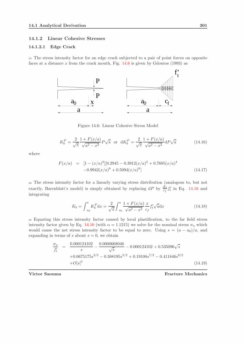
14.1 Analytical Derivation 301
14.1.2 Linear Cohesive Stresses
14.1.2.1 Edge Crack
23 The stress intensity factor for an edge crack subjected to a pair of point forces on oppositefaces at a distance x from the crack mouth, Fig. 14.6 is given by Gdoutos (1993) as
a0 a0a
P
P
xa
f’t
cf
Figure 14.6: Linear Cohesive Stress Model
KPb =
2√π
1 + F (x/a)√a2 − x2
P√
a or dKPb =
2√π
1 + F (x/a)√a2 − x2
dP√
a (14.16)
where
F (x/a) = [1 − (x/a)2][0.2945 − 0.3912(x/a)2 + 0.7685(x/a)4
−0.9942(x/a)6 + 0.5094(x/a)8 ] (14.17)
24 The stress intensity factor for a linearly varying stress distribution (analogous to, but not
exactly, Barenblatt’s model) is simply obtained by replacing dP by dxcf
f ′t in Eq. 14.16 and
integrating
Kb =
∫ a
a0
KPb dx =
2√π
∫ a
a0
1 + F (x/a)√a2 − x2
x
cff ′
t
√adx (14.18)
25 Equating this stress intensity factor caused by local plastification, to the far field stressintensity factor given by Eq. 14.10 (with α = 1.1215) we solve for the nominal stress σn whichwould cause the net stress intensity factor to be equal to zero. Using s = (a − a0)/a, andexpanding in terms of s about s = 0, we obtain
σn
f ′t
=0.000124102
s− 0.0000668046√
s− 0.000124102 + 0.535096
√s
+0.0675175s3/2 − 0.388195s5/2 + 0.19108s7/2 − 0.411846s9/2
+O[s]5 (14.19)
Victor Saouma Fracture Mechanics

302 SIZE EFFECT
26 Even though s is very small, we can drop the first three terms which are negligibly smallcompared to the others. This is first confirmed by replacing s with 1/(1 + r), and plottingEq. 14.19 with all the terms up to s3/2, and the very same equation with the first three termsomitted, Fig. 14.7. We observe that those two graphs (plotted on a linear scale to enhance thepotential discrepancies) are practically identical, with a small deviation in the high range of r.
5 10 15 20 25 30 35 40 45 50
r
0.1
0.15
0.2
0.25
0.3
0.35
0.4
σ N/f
’ t
Full ExpressionFirst Three Terms Dropped
Figure 14.7: Energy Transfer During Infinitesimal Crack Extension
Hence, we may now justifiably drop the first three terms in Eq. 14.19, and rewrite thisequation as:
σn =0.5351f ′
t√1 + r
(1 +
0.126182
1 + r
)+ O[s]2 (14.20)
=0.5351f ′
t√1 + r
[−0.0728836
(−4.66957 +
1
1 + r
)(2.93828 +
1
1 + r
)]+O[s]3 (14.21)
=0.5351f ′
t√1 + r
[0.357092
(2.21298 +
1
(1 + r)2− 1.46954
1 + r
)
Victor Saouma Fracture Mechanics

14.1 Analytical Derivation 303
(1.26544 +
1
1 + r
)]+ O[s]4 (14.22)
=0.5351f ′
t√1 + r
[−0.769662
(1.16279 +
1
(1 + r)2 − 0.1646991+r
)(−1.21723 +
1
1 + r
)(0.917969 +
1
1 + r
)]+ O[s]5 (14.23)
27 We note that the derived size effect law contains higher order terms than those originallyderived by Bazant through Eq. 16.5.
28 Bazant size effect law is recovered through Eq. 14.20 by dropping the second term in theparenthesis. As to Eq. 14.21-14.23 they definitely contain even higher order terms, Fig. 14.8.
10−3
10−1
101
r10
−1
100
σ N/f’
t
exp to power 3/2exp to power 5/2exp to power 7/2exp to power 9/2
Figure 14.8: Size Effect Law for an Edge Crack with Linear Softening and Various Orders ofApproximation
14.1.2.2 Three-Point Bend Specimen
29 We then turn our attention to a slightly more complex geometry, a three point bend specimen,Fig. 14.9, for which the stress intensity factor is now given by Gdoutos (1993) as:
Ka =PS
BW 3/2
[2.9(a/W )1/2 − 4.6(a/W )3/2 + 21.8(a/W )5/2
−37.6(a/W )7/2 + 38.7(a/W )9/2]
(14.24)
30 The stress intensity factor for an edge crack subjected to a linearly varying cohesive stress(Barenblatt’s type) Kb, Fig. 14.6 was given by Equation 14.18.
Victor Saouma Fracture Mechanics

304 SIZE EFFECT
S
a
f’t f’t
P
W
0 B
Figure 14.9: Three Point Bend Specimen with Linear Cohesive Stresses
As before, equating the two stress intensity factors, solving for σ, substituting s = (a−a0)/a,and expanding in terms of s about s = 0, we obtain
σ
f ′t
= −0.000067298
s+
0.0000597828√s
+ 0.000067298 + 1.06378√
s
+8.32667 × 10⁻¹⁷s + 0.132783s3/2 + O[s]2 (14.25)
As for Eq. 14.19, it can be shown that we can retaining the terms in s1/2 and s3/2 without lossof accuracy, and thus obtain
σn =1.06738f ′
t√1 + r
(1 +
0.124401
1 + r
)+ O[s]2 (14.26)
31 Again, this newly derived size effect law for a three point bend beam with a linearly varyingcohesive stress along the fracture process zone is to be contrasted with Eq. 16.5. Should wedrop the second term within the parenthesis, then and only then we will recover an equationanalogous to Eq. 16.5.
14.2 Discussion
14.2.1 Comparison with Experimental Data
32 In order to assess the results, we closely examine experimental size effects tests on three pointbending concrete specimens as reported in Table 1.5.2 of Bazant, Z. and Planas, J. (1998).
Table 14.1 gives the compressive strength and Bf ′t. For the sake of simplification, we assume
f ′t = 0.1f ′
c, and thus determine the experimental value of the B coefficient.The average experimentally determined value is 1.39 (with a standard deviation of 0.61),
and compares relatively well (given the assumption of a Barenblatt cohesive stress model) withthe analytically derived value of 1.07 in Eq. 14.26. Interestingly enough, we note that theexperimentally determined B value is clearly inversely proportional to the nominal specimensize D0.
Victor Saouma Fracture Mechanics

14.2 Discussion 305
Series f ′c Bf ′
t B D0 ReferenceMPa MPa mm
A5 46.8 2.9 0.62 212. (Walsh 1972)A2 35.4 2.8 0.79 157. (Walsh 1972)A4 15.6 1.7 1.09 126. (Walsh 1972)B1 34.1 6.0 1.76 60. (Bazant and Pfeiffer 1987)A6 32.7 4.1 1.25 55. (Walsh 1972)A1 23.1 4.5 1.95 36. (Walsh 1972)A3 14.3 3.2 2.24 34. (Walsh 1972)
Table 14.1: Experimentally Determined Values of Bf ′t, (Bazant, Z. and Planas, J. 1998)
14.2.2 Implications
33 We can rewrite Eq. 16.5 as
f∗t =
f ′t√
1 + β=
σN
B, (14.27)
where f∗t is termed the size-reduced-strength and is a characteristic of the entire structure and
not only of the material.
34 Undoubtedly the size effect law is a very elegant generalized model for concrete fracture.It attempts to provide a unified mathematical model for concrete cracking by merging twodifferent approaches. Furthermore, it has been experimentally validated with numerous tests,many of which involved uncracked (initial) structures.
35 Despite its general appeal, this model calls for the following comments:
1. The size effect law can be plotted on a log-log scale, as shown in Fig. 14.10, with σn
versus size d.
2. For structures of a small size relative to the size of aggregate, i.e for small λ, the value ofλλ0
in Eq. 14.27 may be neglected in comparison to 1, yielding f∗t � f ′
t, and the classicalstrength criterion governs.
3. Again for small structures (small β), B = σN
f ′
tand can be determined from plastic limit
analysis.
4. For structures with very large size compared to aggregate size, λλ0
� 1. Thus Eq. 14.27
reduces to f∗t � f ′
t
√λ0λ , and we see that “For very large concrete structures, such as dams
(or large rock masses), Eq. 14.27 asymptotically approaches the size effect of linear elasticfracture mechanics”.
Victor Saouma Fracture Mechanics

306 SIZE EFFECT
Figure 14.10: Size Effect Law
5. In general, Eq. 14.27 represents a gradual transition from the strength criterion for smallstructures to linear elastic fracture mechanics for large structures.
6. To assess the size effect law, geometrically identical specimens, but with different sizesmust be tested. Then Eq. 14.27 can be cast in the form:
Y = a + bλ =1
σ2N
, (14.28)
where a = 1B2 and b = 1
B2λ0. From statistical regression analysis, the intercept a, and the
slope b can be determined, and then B = 1√a
and λ0 = ab
7. If λλ0
= β is less than 0.1, then a strength criterion must be used, and if β is greater than10, then a LEFM criterion is to be used. Note that those are arbitrary guidelines.
8. The point of intersection of the two asymptotes corresponds to β = 1.
9. At no stage did we have to introduce (explicitly or implicitly) any LEFM equation (inthe sense of a stress singularity at the crack tip).
10. The square root relationship between f∗t and d (through λ) comes from:
• an appropriate choice of the normalizing parameter for the crack length a in definingα1 and α2.
• expression for GF in terms of the square of f ′t in Eq. ??. Although it is correct to
directly relate GF to the area under the uniaxial stress strain curve (a measure ofthe energy required to produce a unit surface), the square component is again notlinked to LEFM.
Victor Saouma Fracture Mechanics

14.2 Discussion 307
Column Buckling Size Effect
Euler Equation LEFMSlenderness ratio Size
Plastic failure Plastic failureInelastic stresses Cohesive stressesInelastic Buckling NLFM
Column Equation (SSRC) Size Effect law (Bazant)
σcr = σy
[1 − σy
4π2E
(KLrmin
)2]
σn =Bf ′
t√1+β
Table 14.2: Size Effect Law vs Column Curve
11. It can be shown, (Bazant and Cedolin 1991) that the fracture energy GF can be recoveredfrom the Size Effect Law
12. There is a strong analogy between the size effect and column buckling, Fig. 14.11, Table14.2.
ydσ
ydσ
kLr
kLr
2σ = π E
( )2
E T < E
ε
σ
rσ
σ Euler Buckling (Linear Elastic)
Gross Yielding
InelasticBuckling
Proportional Limit Proportional Limit
E
Effect of Residual Stresses
Figure 14.11: Inelastic Buckling
14.2.3 LEFM vs NLFM Analyses
36 Ideally, we should extend the analytical solution to encompass Hillerborg’s model as appliedto a three point bending concrete specimen. To the best of the author’s knowledge only tworesearchers addressed this complex nonlinear problem. Xu and Reinhardt (2000) developed aclosed form solution, albeit an empirical one (as termed by its authors). Another solution was
Victor Saouma Fracture Mechanics

308 SIZE EFFECT
presented by Karihaloo (1999) who again indirectly solved this problem, but with some ratherrestricting assumptions by enforcing a zero net stress intensity factor at the tip of the FPZ.Because of the restrictions imposed to those two solutions, the authors have not consideredthem in this study.
37 In a nonlinear fracture mechanics analysis the crack growth criteria is stress based, i.e thecrack tip maximum tensile stress can not exceed the (non-zero) concrete tensile strength. Al-ternatively, in an LEFM analysis, we can set as a criteria a zero fracture toughness.
38 Whereas both criteria are readily accepted by the research community, practicing engineershave difficulties in accepting a non-zero tensile strength (hence rendering a NLFM analysisimpossible), but can accept a small (preferably zero) fracture toughness, (Federal RegulatoryCommission 1991) (in this context, the double-K method might be more acceptable to practicingengineers than solutions based on GF and a non-zero f ′
t). By the same token, a NLFM analysisshould extend the fracture process zone to the point where the stress singularity no longerexists.
39 In order to highlight the duality between a zero fracture toughness criteria in an LEFManalysis, and a non-zero tensile strength criteria in a NLFM analysis a series of numericalanalysis were performed. Considering a three point bend specimen, with GF =100 N/m, f ′
t=2MPa, S/W = 8, a/W = 0.6, s0=100 mm, beams with s0, 10s0, 50s0 and 100s0 were analyzedusing the code Merlin (Saouma, Cervenka and Reich 1997–2004). Through those analyses, thetwo stress intensity factors Ka (caused by the external load) and Kb (caused by the cohesiveHillerborg’s stress) were determined. Whereas contour integral techniques should be favored,one should be careful to leave a small zone at the tip of the crack traction free, otherwise theJ integral will be equal to zero. Hence, in the context of this analysis (with surface traction onthe crack faces) we used singular elements.
40 In each analysis, Pmax corresponded to the onset of unstable crack growth (based on tensilestress at the crack tip), and the corresponding stress intensity factor Ka+b were determined. Itshould be noted that in our implementation of the interface element (based on the extendedHillerborg’s model) pre-peak crack opening can occur. This results in a nonlinear pre-peakload-cod curve.
41 Whereas the variation of Pmax with respect to s was indeed according to Bazant’s size effectlaw, the net stress intensity factors at Pmax ranged between 0.05 and 1.5 MPa
√mm. Given
that a representative value for the fracture toughness of concrete is about 1 MPa√
m or 31MPa
√mm, the net stress intensity factor can be considered as essentially zero. These values
should be independent of the tensile strength, as a higher f ′t would result in a larger external
load, and a higher Ka, but also in a higher (negative) Kb caused by the cohesive stresses.Indeed, when the tensile strength was increased from 2 MPa to 4 MPa, Pmax was about twicethe original values, however there was no discernable variation in Ka+b.
42 Thus, we conclude that for all practical purposes a NLFM analysis yields a very small non-zero stress intensity factor in comparison with fracture toughness. Hence, practicing engineers
Victor Saouma Fracture Mechanics

14.3 Conclusion 309
who accept a zero fracture toughness LEFM analysis should be reassured that a non-zero tensilestrength in the context of a NLFM is, for all practical purposes, identical.
14.3 Conclusion
43 The size effect law is rederived through a balancing of far-field induced stress intensity factorswith those caused by the cohesive stresses. Hence, a direct relationship between plasticity andLEFM to the size effect law is presented. It is shown that the shape of the cohesive stressesis irrelevant, that the B coefficient can, albeit with some restriction, be analytically derived.Furthermore, in the context of the reported derivation, it is shown that not only quasi-brittlematerials exhibit a size effect, but elasto-plastic ones (such as metals) too.
44 Finally, it was also shown that a NLFM analysis with a non-zero tensile strength is practicallyidentical to a LEFM analysis with zero fracture toughness.
Victor Saouma Fracture Mechanics

310 SIZE EFFECT
Victor Saouma Fracture Mechanics

Chapter 15
FRACTALS, FRACTURES andSIZE EFFECTS
Adapted from (?)
15.1 Introduction
15.1.1 Fracture of Concrete
There is not yet a standard for concrete fracture testing although several have been proposed(RILEM, 1985). Concrete fracture properties include fracture toughness KIc, characteristiclength lch, brittleness number β, fracture energy GF , crack-tip opening displacement CTOD,and at least three additional parameters that characterize the concrete strain softening curve.
This chapter addresses a technique that uses fractal geometry to determine whether there isany surface indication of the direction of crack propagation in concrete and whether there is acorrelation between fracture properties (KIc and GF , which characterize the material resistanceto cracking) and the roughness of the fracture surface as characterized by the fractal dimensionD. The implications of the fractal nature of the cracked surface on the “true” fracture or surfaceenergy are then discussed.
15.1.2 Fractal Geometry
Although most manmade objects have linear or smoothly curvilinear shapes, natural objects(such as rivers, mountains, clouds, and fractures) are commonly rough, fragmented, or dis-continuous. The apparent randomness of these irregularities, coupled with our bias towardEuclidian geometry, handicapped us in studying and properly modeling such objects until theadvent of fractal geometry (Mandelbrot, 1983) .
By definition, an inherent property of fractal objects is the statistical replication of patternsat different scales; a magnified part of a fractal object is statistically identical to the whole.Hence, Fig. 15.1-A illustrates the generation of a self-similar synthetic fractal curve, the triadic

312 FRACTALS, FRACTURES and SIZE EFFECTS
������
����
�����
�
�
1/3
���� ����
�������� ����
� � � �
1/3 1/3 1/3
Straight line initiator
Fractal generator
Fractal figure (first iteration)
Length of subparts (S)
of fractal generator segments
(A)
� � � � �
r r r r
�
�
�
r
r
���� �
���
� � �� � �
r r rr2
r2
����
�
�
r
(B) (C)
Figure 15.1: (A) Straight line initiator, fractal generator, and triadic Koch curve; (B) QuadraticKoch curve; (C) Modified Koch curve.
Victor Saouma Fracture Mechanics

15.1 Introduction 313
Step N S s Length
1 1 1 1 12 4 1
3 3 43
3 16 19 9 16
9
Table 15.1: Fractal dimension definition
Koch curve.. First, an initiator, which represents an initial geometric form, is defined, then agenerator, which describes a transformation on the initiator, is applied. As the transformationoperation is repeatedly applied to the figure, a fractal curve is generated. For the triadic Kochcurve, we note that at each step the number of line segments is increased by a factor of 4 andthat the length of each new line segment generated is one third the length of line segmentsin the previous generation. This increases the total length of the fractal curve by four thirdsat each step. Thus, as the number of iterations increases, the number of subdivisions N willvary from 1, 4, 16; s = 1
S where S is the scaling factor from 1, 3, 9; and the correspondinglengths will be 1, 4
3 , and 169 . The total length will eventually tend to infinity. The results of
this operation are tabulated in Table 15.1. The fractal dimension D is defined as
D =ln N
ln s, (15.1)
An alternative form of this equation is
N = sD. (15.2)
Note that the Euclidian definition of dimension, that is the topological dimension, is recov-ered if a line is subdivided into equal parts without changing its length. Since N = S in thiscase, D = 1.
In our previous example, we subdivided line segments into four parts, thus N = 4 and weused S = 1/3 or s = 3. This gives a fractal dimension of D = ln 4
ln 3 = 1.2619 for the curve shownin Fig. 15.1-A.
Mandelbrot (1983), offered the following tentative definition of a fractal. A fractal is aset for which the Hausdorf-Besicovitch dimension (D) strictly exceeds the topological dimension(DT ). For the curve shown in Fig. 15.1-A the topological dimension is 1, whereas the Hausdorf-Besicovitch dimension is 1.2619.
Hence, fractal surfaces have DT = 2 and fractal dimensions D > 2. Mandelbrot (1983)showed that, as a rule of thumb, for a set S that is the product of two independent fractalsets S1 and S2 the fractal dimension of S equals the sum of the fractal dimensions of S1 andS2. Hence, if the triadic Koch surface is uniformly extruded along the z direction, the fractaldimension of the surface is S = S1 + S2 = 1.2619 + 1 = 2.2619 (Feder, 1988) provided that wehave two independent fractal sets. Alternatively, if the extrusion is fractal, then D is greaterthan 2.2619.
Victor Saouma Fracture Mechanics

314 FRACTALS, FRACTURES and SIZE EFFECTS
15.1.3 Numerical Determination of Fractal Dimension
Although the fractal dimension D of synthetic curves can be readily determined analytically,the dimension of arbitrary curves requires the use of numerical methods. Three of the mostcommonly used methods for measuring the fractal dimension of surface roughness are reviewedhere.
Ruler Method: In the ruler method (Aviles and Scholz, 1987, and Mandelbrot, 1983), adivider (that is ruler) of given length S is used to determine the total length of the curve.Note that no fractional lengths can be taken. Thus, for a given ruler length, the curvelength L is given by SN where N is an integer. This operation is repeated for a ruler ofsmaller and smaller length S, and the fractal dimension is given by
N = (1
S)D
= sD, (15.3)
S · N︸ ︷︷ ︸L
= S · ( 1
S)D︸ ︷︷ ︸
S1−D
ln L = (1 − D) ln S. (15.4)
Box Method: The box method is used in this study to measure the fractal dimension of thefracture roughness profiles. In principal, the method is simple; a sequence of grids, eachhaving a different cell size, is placed over maps of the fracture traces and the number ofcells intersected by fracture traces counted, (Barton et.al., unpublished). The numberof grid cells intersected by the profile N is then plotted on a log-log scale with respect tothe inverse of the grid cell size s = 1
S . If a linear relationship is found, then the object issaid to be fractal within the specified range of cell sizes and the fractal dimension is theslope of the line.
The box method, as well as the ruler method, is strictly applicable to self-similar datasets. Fracture roughness profiles in rock have been shown to be self-affine (Brown 1987,1988). Brown’s analysis shows that application of the ruler method to self-affine datasets yields the correct fractal dimension only when the maximum ruler length used is lessthan the crossover length, which is defined as the ruler length beyond which the rulermethod will always yield a fractal dimension of approximately one. Brown (1987, 1988)shows that the crossover is the length where the standard deviation of amplitude is equalto the wavelength, which for our profiles is approximately 8 × 10⁻² meters. We expectthe box method to exhibit a crossover length when applied to self-affine data sets such asour fracture surface profiles. Therefore, in this study we limited the largest box size to8 × 10−2 m.
Slit Island Method: Whereas the preceding two methods measure the fractal dimension offracture profiles (1 < D < 2), the Slit Island method is applicable to fractal surfaces(2 < D < 3). For each contour line of different elevation over the fracture surface, the
Victor Saouma Fracture Mechanics

15.1 Introduction 315
perimeter L and the area A are determined and then plotted on a log-log scale. Thefractal dimension is then be obtained from (Feder, 1988)
A = L2
D−1 . (15.5)
15.1.4 Correlation of Fractal Dimensions With Fracture Properties
Fractal analysis is a simple and powerful tool for quantifying complex physical quantities. Ithas been used in numerous fields, ranging from clustering of co-citations in scientific papers(Van Raan, 1990) to earthquake prediction (Levi, 1990).
The roughness and irregularities of fractured surfaces make them ideal candidates for afractal analysis. Indeed, as pointed out by Cahn (1989), fracture and fraction (fractals havefractional dimensions) have the same latin root fractus, which means to break and to createirregular fragments. This potential correlation has been the subject of numerous studies, whichhave yielded conflicting conclusions.
In the first study of fracture surfaces, Mandelbrot et al. (1984) showed that not onlyare cracked metallic surfaces (300-grade maraging steel) fractal but their fractal dimensionis inversely proportional to the impact energy determined by the Charpy impact test (itselfproportional to fracture toughness). Through simulation of a numerical model for fracturebased failure of a polymeric, Termonia and Meakin (1986) showed that the synthetic fracturesurfaces are also fractal and that the fractal dimension has a universal value of D = 1.27±0.02.More recently, Peng and Tian, (1990) showed through a simple theoretical kinetic model whichsimulates crack propagation, that the resulting fracture surface is fractal and that its dimensiondepends on the material’s elastic constants.
Although most researchers have found that fractured surfaces are fractal, Underwood andBanerji (1986), using AISI4340 steel specimens, did not detect a linear fractal curve andconstant D but rather a reverse sigmoidal curve and variable D.
Mecholsky et al. (1989) concluded that the toughness increases with the roughness for sixdifferent alumina materials and five glass-ceramics having different microstructures and that
the fracture toughness is directly related to the fractal dimension KIc = Ea120 D∗ 1
2 , where D∗ isthe fractional part of D, E is the elastic modulus, and a0 a parameter having the units of length.Similar results were subsequently obtained for single crystal silicon (Tsai and Mecholsky, 1991)and for polystyrene fracture surfaces (Chen and Runt, 1989). More recently, Mecholsky andFreiman (1991) showed that there is a spatial variation of D along the length of the crackreflecting crack initiation and, later on, microbranching.
Discrepancy between results was recently pointed out by Cahn (1989), who noted thatthe relationship between fracture roughness as quantified by fractal dimension and fracturetoughness is diametrically opposite for ductile fracture (maraging steel) and for brittle fracture(chert, and polycristalline ceramics).
Recently, a fractal approach was applied to the fracture of rocks and soil. Heping (1987)postulated that the surface area of a crack for which the critical energy release rate Gc =dUdA is determined, should be adjusted to reflect the rough nature of the surface rather thanthe flat nominal surface. This would then systematically result in fracture toughness values
Victor Saouma Fracture Mechanics

316 FRACTALS, FRACTURES and SIZE EFFECTS
(KIc =√
GcE′) that would increase with fractal dimension. Similarly, Mosolov (1991) hasshown that for fractal cracks, the J integral ceases to be an invariant. Mecholsky and Mackin(1988) correlated the fracture toughness of Ocala chert (flint) with the fractal dimension anddetermined that one increased with the other. Chelidze and Gueguen (1990) showed that thefractal dimension increases with the surface energy (and hence the fracture toughness) of rocks.For fractures in soils, Young and Crawford (1992) determined that fracture profiles are fractal,with fractal dimensions very close to one.
Winslow (1985) showed through X-ray scattering techniques that, on the microscopic level,hydrated cement paste is fractal and has a fractal dimension of about 3.
All of the reported studies concern themselves with metals, polymers, rocks, or cementpastes, and only limited research has been reported in the fractal analyses of cracked concretesurfaces. Saouma et al. (1990) showed that cracked concrete surfaces are fractal. Issa et al.(1992), based on two-dimensional surface studies, found that the fractal dimension D variesfrom 2.1 to 2.22 and increases with aggregate sizes. Most recently, Lange et al. (1993) inves-tigated the correlation between fracture roughness and fracture toughness, fractal dimensionsand other physical properties. They report a fractal dimension of 2.087 for cement paste and2.117 for fine mortar, and an increase between fractal dimension and fracture toughness.
Finally, it should be pointed out that it has been recently hypothesized that there is auniversal value (2.1 < D < 2.3) for the fractal dimension of fractured surfaces (Bouchaud et al.1990) . This hypothesis was more recently strengthened by the finding of Maløy et al. (1992),who tested both ductile and brittle materials and reported a universal fractal dimension ofD = 2.11 ± 0.006.
15.2 Experimental Procedure
15.2.1 Fracture Testing
As part of a study on the applicability of fracture mechanics to the failure analysis of concretedams by Saouma et al. (1991) , a series of wedge splitting (WS) tests was performed onspecimens 3 and 5 ft long (Fig. 15.2), 16 in. thick and with maximum aggregate sizes up tothree inches1. as given in Table 15.2.
The effects of both aggregate size and the type of aggregate (crushed subangular as opposedto river rounded) were studied, as well as the effect of cold-joints.
In the WS experiments, the primary deformation measured was the crack–mouth openingdisplacement (CMOD), which also provided the feedback control to achieve a constant rateof 1.0-μm/sec for the CMOD. Through this configuration, stable crack growth with structuralpost-peak response was achieved. During the test both vertical load and CMOD were monitoredand recorded. Finally, unload/reload cycles were performed to monitor change in specimencompliance from which the effective crack length aeff was then calculated.
1Since all experiments and data reduction were performed using U.S. customary units, the following conver-sions factors should be considered: 1 in.=2.54 cm; 1ft=30.48 cm; 1 psi=689.48 Pa; 1 ksi
√in=0.910 Mpa
√m; 1
lb/in.=175.44 N/m.
Victor Saouma Fracture Mechanics
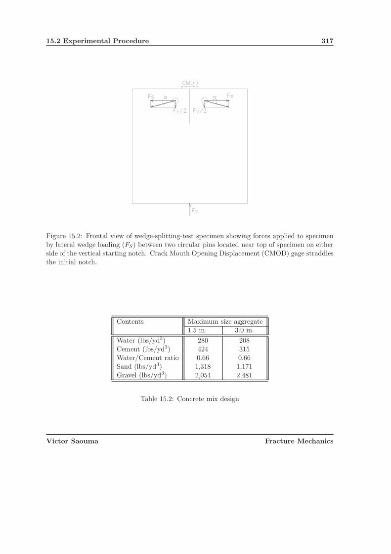
15.2 Experimental Procedure 317
Figure 15.2: Frontal view of wedge-splitting-test specimen showing forces applied to specimenby lateral wedge loading (FS) between two circular pins located near top of specimen on eitherside of the vertical starting notch. Crack Mouth Opening Displacement (CMOD) gage straddlesthe initial notch.
Contents Maximum size aggregate1.5 in. 3.0 in.
Water (lbs/yd3) 280 208Cement (lbs/yd3) 424 315Water/Cement ratio 0.66 0.66
Sand (lbs/yd3) 1,318 1,171Gravel (lbs/yd3) 2,054 2,481
Table 15.2: Concrete mix design
Victor Saouma Fracture Mechanics

318 FRACTALS, FRACTURES and SIZE EFFECTS
Range Precision
X 24 .0021Y 60 .0013Z 5 .005
Table 15.3: Range and resolution of the profilometer (inches)
SPECIMEN SIZE 3 ft 5 ft
Profile 0◦ 16.0 in. 26.67 in.length 90◦ 15.0 in. 15.0 in.
±45◦ 17.0 in. 20.0 in.
Resolution 0◦ 160 /in. 160/in.of 90◦ 192/ in. 192/in.
readings ±45◦ 175/ in. 175/in.
Spacing 0◦ 4.0 in. 4.0 in.between 90◦ 4.0 in. 4.0 in.profiles ±45◦ 2.0 in. 4.0 in.
Table 15.4: CHECK Mapped profile spacing, orientation, and resolution for the two specimensizes investigated
15.2.2 Profile Measurements
A fully automated profilometer (Saouma et al., 1990) , which scans the surface by means of amotorized computer-controlled placement of a linear variable differential transformer (LVDT),was used to determine crack profile with an average resolution of 0.001 in. the precision shownin Table 15.4. The LVDT is seated on a composite bushing that slides along two parallel,ground-steel rods which are rigidly attached to a second bushing. The second bushing traversesa second pair of rods, which, in turn, are mounted at right angles with respect to the firstset of rods. The entire system is placed on a rigid steel base over the specimen. Movementsof the two bushing sets are controlled by two-worm gear and stepped-motor assemblies suchthat the LVDT can travel along any preprogrammed path in the X − Y plane. Two separatecomputers are used, the first to control positioning of the LVDT, the second to record and storeits reading (following reception of a signal from the first one). Finally, for each specimen profile,measurements along the four principal orientations (at 45◦ increments) were recorded in orderto assess potential geometric anisotropy in fractal dimensions as shown in Fig. 15.3.
15.2.3 Computation of Fractal Dimension
Following preliminary tests, it was determined that the box method yielded more consistentresults than the ruler method, and hence it was adopted. The box method can be applied to
Victor Saouma Fracture Mechanics
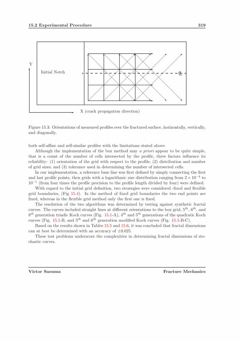
15.2 Experimental Procedure 319
Initial Notch�
�
Y
X (crack propagation direction)
�
�
�
�� � � �
��
��
��
��
��
���
��
��
��
��
��
���
��
��
��
��
��
���
��
��
��
��
��
���
CL
Figure 15.3: Orientations of measured profiles over the fractured surface, horizontally, vertically,and diagonally.
both self-affine and self-similar profiles with the limitations stated above.Although the implementation of the box method may a priori appear to be quite simple,
that is a count of the number of cells intersected by the profile, three factors influence itsreliability: (1) orientation of the grid with respect to the profile; (2) distribution and numberof grid sizes; and (3) tolerance used in determining the number of intersected cells.
In our implementation, a reference base line was first defined by simply connecting the firstand last profile points, then grids with a logarithmic size distribution ranging from 2× 10⁻⁴ to10−1 (from four times the profile precision to the profile length divided by four) were defined.
With regard to the initial grid definition, two strategies were considered -fixed and flexiblegrid boundaries, (Fig 15.4). In the method of fixed grid boundaries the two end points arefixed, whereas in the flexible grid method only the first one is fixed.
The resolution of the two algorithms was determined by testing against synthetic fractalcurves. The curves included straight lines at different orientations to the box grid; 5th, 6th, and8th generation triadic Koch curves (Fig. 15.1-A), 4th and 5th generations of the quadratic Kochcurves (Fig. 15.1-B, and 5th and 6th generation modified Koch curves (Fig. 15.1-B-C).
Based on the results shown in Tables 15.5 and 15.6, it was concluded that fractal dimensionscan at best be determined with an accuracy of ±0.025.
These test problems underscore the complexities in determining fractal dimensions of sto-chastic curves.
Victor Saouma Fracture Mechanics

320 FRACTALS, FRACTURES and SIZE EFFECTS
������
������
��������
����
������������
��������
A B
Figure 15.4: Typical grid overlying an object. Dashed lines indicate adjustable sidFixed gridboundaries; B, Flexible grid boundaries.
Angle of Grid sizeinclination 40 points 300 points 1000 points
0◦ 1.000 1.000 1.0005.0◦ 1.030 1.013 1.00610.0◦ 1.048 1.017 1.00815.0◦ 1.057 1.017 1.00820.0◦ 1.062 1.017 1.00825.0◦ 1.078 1.020 1.00930.0◦ 1.062 1.017 1.00735.0◦ 1.068 1.017 1.00740.0◦ 1.080 1.019 1.00845.0◦ 1.000 1.000 1.000
Table 15.5: Computed fractal dimensions of a straight line with various inclinations
Victor Saouma Fracture Mechanics

15.3 Fractals and Fracture 321
Fixed grids Flexible grids
Koch curve Generation D Grid D Grid Theoreticaltype size size Value
Triadic 5th 1.377 15 1.305 500Triadic 6th 1.313 64 1.307 500 1.262Triadic 8th 1.285 647 1.296 500
Quadratic 4th 1.410 17 1.477 500 1.500Quadratic 5th 1.477 93 1.486 500
Modified 5th 1.188 93 1.190 500 1.161Modified 6th 1.177 401 1.186 500
Table 15.6: Computed fractal dimensions for various synthetic curves
15.3 Fractals and Fracture
The fracture surfaces of our specimens are fractal for grid sizes ranging from 2×10−3.2 to 10−2.1
m (Fig. 15.5). The average fractal dimension of approximately 1.1 compares exactly with theone determined experimentally for concrete by Issa et al., (1992), (D = 2.2
2 = 1.1, assumingthat we do have two independent and orthogonal fractal sets as partially supported by Table15.7 and by Long et al. (1991)) and with the universal value of 2.11 proposed for fracturesurfaces by Maløy et al. (1992) . The division by two to obtain the profile fractal dimensionfrom a surface fractal dimension was discussed previously, and is justified by the fractal natureof orthogonal profiles having almost identical fractal dimensions (as will be discussed following).
Having confirmed the fractal nature of the cracked surfaces, three important questions arise:(1) what is the spatial variation of the fractal dimension; (2) is there a correlation betweenfractal dimension and fracture properties for concrete; and (3) how do the results for concretecompare with other materials?
15.3.1 Spatial Variation of the Fractal Dimension
The spatial variation of the fractal dimension was investigated with particular attention to the(1) location and length of the profile within the width of the crack front; (2) the orientation ofthe profile with respect to the direction of crack propagation; and (3) specimen and aggregatesizes and aggregate angularity.
D versus Profile Location and Length: Variation in fractal dimension as a function of pro-file location and profile length was studied for a series of profiles oriented parallel to thedirection of fracture propagation on a single fracture specimen because it was postulatedthat:
1. Different D values across the thickness might be obtained due to the near planestress condition on the edge of the specimen and the near plane strain condition at
Victor Saouma Fracture Mechanics

322 FRACTALS, FRACTURES and SIZE EFFECTS
2.0 2.5 3.0 3.5-Log of Box Size (in meters)
1.5
2.0
2.5
3.0
Log
(N)
Box Sizes vs Number of Occupied Boxesfor a Typical Fractured Surface
Figure 15.5: Plot of box counting method applied to the profile of a typical fractured concretespecimen. Number of occupied boxes (N) is plotted versus box size. Slope of line fit to data isthe fractal dimension (D).
Victor Saouma Fracture Mechanics

15.3 Fractals and Fracture 323
Specimen Profile Profile Distance from Centerline Average σD%direction 1 in. 3 in. 5 in. 7 in.
3-ft specimens of 1.5-in. MSA
0◦ 1.096 1.118 1.098 1.113 1.106 1.1A 90◦ 1.087 1.115 1.101 1.088 1.098 1.1
+45◦ 1.096 1.100 1.104 1.123 1.106 1.1−45◦ 1.073 1.109 1.090 1.097 1.092 1.1
0◦ 1.096 1.118 1.064 1.112 1.097 2.2B 90◦ 1.109 1.100 1.088 1.133 1.107 1.7
+45◦ 1.112 1.111 1.073 1.125 1.105 2.0−45◦ 1.094 1.085 1.096 1.085 1.090 0.5
0◦ 1.130 1.128 1.094 1.115 1.117 1.5C 90◦ 1.092 1.098 1.126 1.106 1.105 1.3
+45◦ 1.108 1.087 1.122 1.105 1.105 1.3−45◦ 1.113 1.127 1.101 1.102 1.111 1.1
3-ft specimens of 3.0-in. MSA
0◦ 1.099 1.107 1.084 1.097 1.097 0.9A 90◦ 1.123 1.107 1.087 1.129 1.111 1.7
+45◦ 1.084 1.071 1.089 1.114 1.089 1.7−45◦ 1.148 1.115 1.094 1.123 1.120 2.0
0◦ 1.147 1.096 1.123 1.069 1.109 3.0B 90◦ 1.116 1.127 1.100 1.165 1.127 2.5
+45◦ 1.104 1.111 1.083 1.110 1.102 1.2−45◦ 1.094 1.087 1.107 1.115 1.101 1.1
0◦ 1.118 1.098 1.113 1.106 1.109 0.8C 90◦ 1.115 1.101 1.088 1.098 1.100 1.0
+45◦ 1.100 1.104 1.123 1.106 1.108 0.9−45◦ 1.109 1.090 1.097 1.092 1.097 0.8
Table 15.7: Fractal dimension D versus profile orientations
Victor Saouma Fracture Mechanics

324 FRACTALS, FRACTURES and SIZE EFFECTS
Distance from Zone of analysisspecimen First Second Third Fourth First Secondcenterline quarter quarter quarter quarter half half
1 in. 1.118 1.120 1.073 1.083 1.126 1.0933 in. 1.128 1.106 1.111 1.150 1.121 1.1195 in. 1.118 1.080 1.082 1.082 1.084 1.0757 in. 1.110 1.099 1.113 1.119 1.100 1.124
Table 15.8: Fractal dimension for various profile segments and distances from centerline inspecimen S33A
the center.
2. Different D values along the length may be obtained due to the lack of a fullydeveloped process zone in the early part of the crack surface.
Assuming a linear relationship between fractal dimension D and the profile’s distance xfrom the centerline,
D = a + bx (15.6)
it was observed that in most cases b is negative, implying a reduction in fractal dimensionD as the profile moves from the centerline to the edge. This was confirmed by visualinspection of the cracked surfaces, which showed that the center of the cracked surfaceappears to be rougher than the edge.
When the fractal dimensions of the same specimen were determined over different partsof the length (Table 15.8), it was observed that in most cases D is greater over the firsthalf than over the second half. In most cases D is greater in the first quarter than inthe fourth one. Even though the difference is quite small (more supporting experimentaldata is needed to fully address this point), it may be caused by the presence of a fullydeveloped process zone in the first half as opposed to the second one.
D versus Orientation of Profile: It has been speculated that the direction of crack propa-gation might affect the value of D. If this is correct, then it should be possible throughpostmortem investigation of a cracked surface to determine the direction of fracture prop-agation.
We concluded by examination of the results (Table 15.7), that there is no apparent corre-lation between the fractal dimension and the profile orientation. It should be noted thatLong et al. (1991) found that there is such a correlation for metals.
D versus Specimen Size, Aggregate Size, and Aggregate Type: Comparing the fractaldimension D obtained from 3- and 5-ft-long specimens (Table 15.9), there is a clear indi-cation that the longer the specimen size, the lower the fractal dimension everywhere onthe fracture surface. This may result from the correlation between D and KIc (discussed
Victor Saouma Fracture Mechanics

15.3 Fractals and Fracture 325
Distance from centerline Fractal dimension GF , KIc [psi√
in]Specimen 1 in. 3 in. 5 in. 7 in. Average σD% [lb/in] Average σK%
3-ft specimens of rounded 1.5-in. MSA
S32A 1.096 1.094 1.096 1.112 1.100 0.8 1.28 812. 10.0S32B 1.096 1.118 1.064 1.112 1.098 2.2 1.17 909. 5.5S32C 1.130 1.128 1.094 1.115 1.117 1.5 1.36 1,004. 11.3
Average 1.107 1.113 1.085 1.113 1.105 1.27 908
3-ft specimens of rounded 3.0-in. MSA
S33A 1.099 1.107 1.084 1.097 1.097 0.9 1.21 901. 6.3S33B 1.147 1.096 1.123 1.069 1.109 3.0 1.26 862. 6.4S33C 1.118 1.098 1.113 1.081 1.103 1.5 1.40 1,166. 7.7
Average 1.121 1.100 1.107 1.082 1.103 1.29 976
3-ft specimens of 1.5-in. MSA (subangular basalt aggregate)
SS32A 1.084 1.089 1.096 1.052 1.080 1.8 1.73 1,274. 9.6SS32B 1.090 1.077 1.096 1.076 1.085 0.9 1.42 1,137. 12.3
Average 1.087 1.083 1.096 1.064 1.083 1.57 1,206.
5-ft specimens of rounded 1.5-in. MSA
S52A 1.085 1.074 1.064 1.069 1.073 0.8 1.17 1,058. 6.9S52B 1.066 1.070 1.072 1.050 1.065 0.9 1.63 1,164. 6.1S52C 1.082 1.067 1.082 1.059 1.073 1.1 1.64 1,138. 3.5
Average 1.078 1.070 1.073 1.059 1.070 1.48 1,120.
5-ft specimens of rounded 3.0-in. MSA
S53A 1.091 1.077 1.088 1.073 1.082 0.8 1.35 893. 13.7S53B 1.037 1.049 1.060 1.048 1.049 0.9 Not applicable
Average 1.064 1.063 1.074 1.061 1.065
5-ft cold joint specimens
CJ52B 1.050 1.045 1.051 1.027 1.043 1.1 0.46 457. 3.3CJ53A 1.051 1.064 1.056 1.050 1.055 0.6 0.76 643. 3.9CJ53C 1.073 1.087 1.070 1.062 1.073 1.0 0.56 567. 2.6
Average 1.058 1.065 1.059 1.046 1.057 0.59 494
Table 15.9: Comparison between D, KIc, and GF for all specimens (MSA, Maximum sizeaggregate)
Victor Saouma Fracture Mechanics

326 FRACTALS, FRACTURES and SIZE EFFECTS
in the next section), that shows bigger specimens yield slightly higher fracture toughnessand smaller D values than smaller specimens.
We find no correlation between D and the aggregate size. This confirms two earlierfindings: (1) fracture toughness values are independent from aggregate sizes (Saouma etal., 1991) and (2) the size-effect law (Bazant, 1984) is not dependent on aggregate sizesas reported in Saouma et al. (1991).
Table 15.9 shows that for 3-ft-long specimens having 1.5-in. maximum size aggregate(MSA), subangular aggregates yielded smaller D values than rounded ones. This corre-lates with our observation that during fracture, the crack circumvented rounded aggre-gates while breaking subangular ones. The former would yield rougher surfaces whereasthe latter would yield tougher ones.
15.3.2 Correlation Between Fracture Toughness and Fractal Dimensions
We now turn our attention to the possible correlation between fractal dimension D and fractureproperties (Table 15.9). This analysis is possible because the specimens were originally testedfor both fracture toughness KIc and fracture energy GF as part of a different research study ofSaouma et al. (1991).
If a correlation could be found, one could determine post mortem important fracture proper-ties, KIc and GF , by measuring roughness of the fracture surface in a forensic study. Table 15.9summarizes fractal and fracture analyses for all specimens, as well as their respective averagesand standard deviations, and Figs. 15.6-A and 15.6-B illustrate the variations of GF and KIc
versus D, respectively.It should be noted that D, GF , and KIc tested higher for concrete than for the cold-jointed
specimens (Table 15.9). This is because of the weak bond between the two layers of concretethat results in relatively smooth surfaces.
Specimens prepared with subangular basalt aggregate had generally higher GF and KIc andlower D. This can be explained by the nature of the fracture surfaces. The fracture plane wentthrough this subangular strong aggregate leaving a relatively smooth surface. The fractureplane went around rounded aggregate, debonding the aggregate from the mortar and yielding arougher surface obtained through less energy. If cold-joint specimens are excluded, D increaseswith a decrease in fracture toughness and energy.
Linear regression between D and both the specific fracture energy GF and the fracturetoughness KIc resulted in the following expressions:
GF = 7.87 − 5.95D lb/in; χ2 = 0.258 (15.7)
KIc = 6, 220 − 4, 766D psi√
in; χ2 = 0.267 (15.8)
Because of the low goodness of fit, great care should be exercised in using the above equations.Table 15.10 summarizes this correlation between fracture properties and fractal dimensions.Excluded are the results obtained from cold joints because these yield both lower fractal di-mensions and lower fracture toughness due to the poor interface bond in those specimens.
Victor Saouma Fracture Mechanics

15.3 Fractals and Fracture 327
1.06 1.07 1.08 1.09 1.10 1.11 1.12Fractal Dimension (D)
0.00
0.20
0.40
0.60
0.80
1.00
1.20
1.40
1.60
1.80
Fra
ctur
e E
nerg
y (lb
/in. G
F)
Fracture Energy vs Fractal DimensionConcrete
Experimental pointGF=7.87-5.95 D
1.06 1.07 1.08 1.09 1.10 1.11 1.12Fractal Dimension (D)
0.0
200.0
400.0
600.0
800.0
1000.0
1200.0
1400.0
1600.0
Fra
ctur
e T
ough
ness
(ps
i sqr
t[in]
; KIC
)
Fracture Toughness vs Fractal DimensionConcrete
Experimental pointKIc=6,220-4,760 D
1.00 1.10 1.20 1.30Fractal Dimension (D)
0.0
1.0
2.0
3.0
4.0
Fra
ctur
e E
nerg
y (lb
/in. G
F)
Fracture Energy vs Fractal DimensionConcrete, Alumina, Ceramics
ConcreteAluminaGlass ceramic
1.00 1.10 1.20 1.30Fractal Dimension D
0.0
1.0
2.0
3.0
4.0F
ract
ure
Tou
ghne
ss (
Mpa
m1/
2 )
Fractal Dimension vs Fracture ToughnessVarious Materials
ConcreteAluminaGlass ceramicsOcal chert (flint)PolystyreneSilicon
Figure 15.6: A-B) GF and KIc versus D; C) GF versus D for concrete (this study), ceramics, andalumina (Mecholsky and Freiman, 1991); D) KIc versus D for concrete (this study); ceramics,and alumina (Mecholsky and Frieman, 1991); Flint (Mecholsky and Mackin, 1988); polystyrene(Chen and Runt, 1989); and silicon (Tsai and Mecholsky (1991)
Victor Saouma Fracture Mechanics
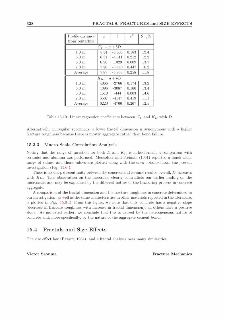
328 FRACTALS, FRACTURES and SIZE EFFECTS
Profile distance a b χ2 Sx.y%from centerline
GF = a + bD
1.0 in. 5.34 -3.605 0.183 12.43.0 in. 6.31 -4.511 0.212 12.25.0 in. 0.26 1.029 0.009 13.77.0 in. 7.26 -5.440 0.447 10.2
Average 7.87 -5.953 0.258 11.8
KIc = a + bD
1.0 in. 4066 -2766 0.174 13.23.0 in. 4396 -3087 0.160 13.45.0 in. 1510 -444 0.003 14.67.0 in. 5507 -4147 0.419 11.1
Average 6220 -4766 0.267 12.5
Table 15.10: Linear regression coefficients between GF and KIc with D
Alternatively, in regular specimens, a lower fractal dimension is synonymous with a higherfracture toughness because there is mostly aggregate rather than bond failure.
15.3.3 Macro-Scale Correlation Analysis
Noting that the range of variation for both D and KIc is indeed small, a comparison withceramics and alumina was performed. Mecholsky and Freiman (1991) reported a much widerrange of values, and those values are plotted along with the ones obtained from the presentinvestigation (Fig. 15.6-).
There is no sharp discontinuity between the concrete and ceramic results; overall, D increaseswith KIc. This observation on the mesoscale clearly contradicts our earlier finding on themicroscale, and may be explained by the different nature of the fracturing process in concreteaggregate.
A comparison of the fractal dimension and the fracture toughness in concrete determined inour investigation, as well as the same characteristics in other materials reported in the literature,is plotted in Fig. 15.6-D. From this figure, we note that only concrete has a negative slope(decrease in fracture toughness with increase in fractal dimension); all others have a positiveslope. As indicated earlier, we conclude that this is caused by the heterogeneous nature ofconcrete and, more specifically, by the nature of the aggregate cement bond.
15.4 Fractals and Size Effects
The size effect law (Bazant, 1984) and a fractal analysis bear many similarities:
Victor Saouma Fracture Mechanics
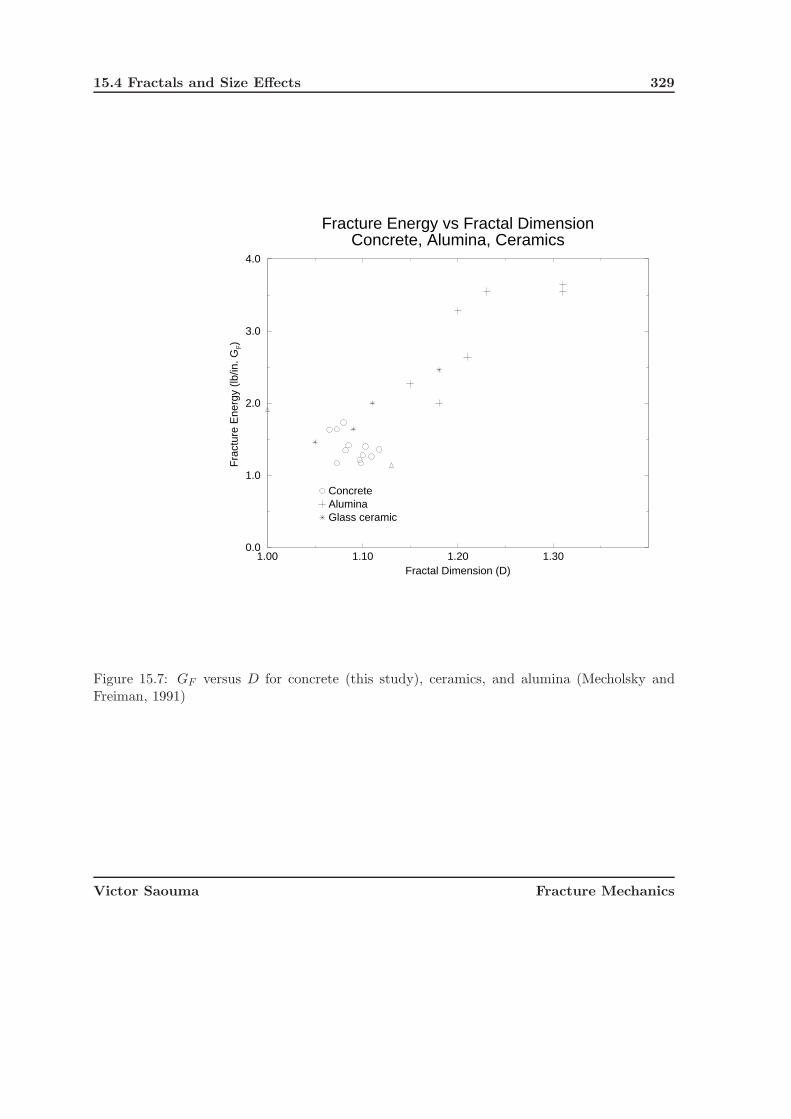
15.4 Fractals and Size Effects 329
1.00 1.10 1.20 1.30Fractal Dimension (D)
0.0
1.0
2.0
3.0
4.0
Fra
ctur
e E
nerg
y (lb
/in. G
F)
Fracture Energy vs Fractal DimensionConcrete, Alumina, Ceramics
ConcreteAluminaGlass ceramic
Figure 15.7: GF versus D for concrete (this study), ceramics, and alumina (Mecholsky andFreiman, 1991)
Victor Saouma Fracture Mechanics

330 FRACTALS, FRACTURES and SIZE EFFECTS
1.00 1.10 1.20 1.30Fractal Dimension D
0.0
1.0
2.0
3.0
4.0
Fra
ctur
e T
ough
ness
(M
pa m
1/2 )
Fractal Dimension vs Fracture ToughnessVarious Materials
ConcreteAluminaGlass ceramicsOcal chert (flint)PolystyreneSilicon
Figure 15.8: KIc versus D for concrete (this study); ceramics, and alumina (Mecholsky andFrieman, 1991); Flint (Mecholsky and Mackin, 1988); polystyrene (Chen and Runt, 1989); andsilicon (Tsai and Mecholsky (1991)
Victor Saouma Fracture Mechanics
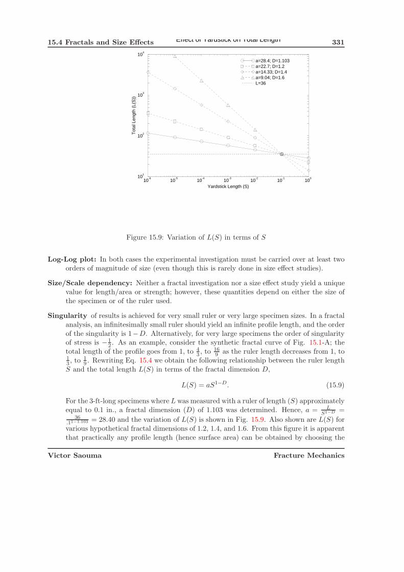
15.4 Fractals and Size Effects 331
10-6
10-5
10-4
10-3
10-2
10-1
100
Yardstick Length (S)
101
102
103
104
Tot
al L
engt
h (L
(S))
Effect of Yardstick on Total Length
a=28.4; D=1.103a=22.7; D=1.2a=14.33; D=1.4a=9.04; D=1.6L=36
Figure 15.9: Variation of L(S) in terms of S
Log-Log plot: In both cases the experimental investigation must be carried over at least twoorders of magnitude of size (even though this is rarely done in size effect studies).
Size/Scale dependency: Neither a fractal investigation nor a size effect study yield a uniquevalue for length/area or strength; however, these quantities depend on either the size ofthe specimen or of the ruler used.
Singularity of results is achieved for very small ruler or very large specimen sizes. In a fractalanalysis, an infinitesimally small ruler should yield an infinite profile length, and the orderof the singularity is 1−D. Alternatively, for very large specimens the order of singularityof stress is −1
2 . As an example, consider the synthetic fractal curve of Fig. 15.1-A; thetotal length of the profile goes from 1, to 4
3 , to 169 as the ruler length decreases from 1, to
13 , to 1
9 . Rewriting Eq. 15.4 we obtain the following relationship between the ruler lengthS and the total length L(S) in terms of the fractal dimension D,
L(S) = aS1−D. (15.9)
For the 3-ft-long specimens where L was measured with a ruler of length (S) approximatelyequal to 0.1 in., a fractal dimension (D) of 1.103 was determined. Hence, a = L
S1−D =36
.11−1.103 = 28.40 and the variation of L(S) is shown in Fig. 15.9. Also shown are L(S) forvarious hypothetical fractal dimensions of 1.2, 1.4, and 1.6. From this figure it is apparentthat practically any profile length (hence surface area) can be obtained by choosing the
Victor Saouma Fracture Mechanics

332 FRACTALS, FRACTURES and SIZE EFFECTS
appropriate ruler length2. This figure also illustrates how a small variation in fractaldimension D results in substantially larger L(S).
In determining the correct surface area, reference is made to the surface area obtainedthrough measurements with a ruler of size S0. From Eq. 15.9, the correct profile lengthLD is given by
L∗ = (S∗
S0)(1−D)L0, (15.10)
where L0 is the length measured with S0.
We hypothesize that
limd→∞
PSEL = limS→′
PF, (15.11)
where PSEL and PF are selected properties obtained from the size effect law and from afractal analysis, respectively. In the former, this entails testing of various similar specimenswith subsequent extrapolation to infinity through the size effect law; in the latter it entailscareful analysis of just one specimen using various rulers lengths.
In order to validate the former hypothesis we consider the fracture energy GF for which thefollowing relation holds
limd→∞
GF = Gc =K2
Ic
E. (15.12)
For 1.5-in. maximum size aggregates in 3-ft-long specimens, the following overall averagevalues were determined (Saouma et al. 1991): GF =1.37 lb/in., KIc=.929 Ksi
√in and E= 2,460
Ksi. Using Eq. 15.12 we determine Gc = .9292
2,4601, 000 = 0.35 lb/in. which is much lower thanGF .
To explain this discrepancy through fractal interpretation, recall that GF is defined as theenergy required to create a unit surface area. The total energy experimentally consumed isdetermined from the area under the load-displacement curve, but how do we define the crackedsurface area?
Traditionally, the nominal surface area has been used (RILEM 1985), and this approach,although justified within the context of a finite element analysis where the roughness of thecracked surface is not accounted for, however may not yield the correct material GF . Aspointed out by Heping (1987), the roughness of the surface should be accounted for, whichwould increase the surface area and thus reduce GF . For a surface area, Eq. 15.10 becomes
A∗ =
(S∗ × S∗
S0 × S0
)(1−D)
A0
=
(S∗
S0
)2(1−D)
A0. (15.13)
2Ironically, this singularity is reminiscent of the one associated with the recovery of (singular) crack tip stressesin terms of the finite element mesh size used; the smaller the crack tip element size, the larger the computedstress.
Victor Saouma Fracture Mechanics

15.4 Fractals and Size Effects 333
S0 S∗
“Macro”: sand “Micro”: C-S-H
#100 # 200 20μm 10μm.0059 in. .0029 in. .0008 in. .0004 in.
1. 2.79 3.22 4.18 4.78.25 2.12 2.44 3.16 3.62.1 1.76 2.03 2.63 3.02
Table 15.11: Amplification factors for fractal surface areas with D = 1.1.
Recall that S0 is the size of the ruler with which L0 was determined (in our case 0.1 in.) and thatS∗ is a threshold or characteristic smallest length scale such as the size of an atom, molecule,or crystal. This quantity is referred to as a monomers by Feder (1988) and is associated withthe physical structure of the surface.
For concrete S∗ can be determined either “macroscopically” as the size of#100 or #200ASTM sieves, with respective sizes of 0.0059 and 0.0029 in. Alternatively, S∗ can be determinedon the basis of a “microscopic” scale associated with the approximate size of the calcium silicatehydrate (C-S-H), which is approximately 10-20μm (0.0004-0.0008 in). Table 15.11 illustratesthe amplification factor for a surface area on the basis of Eq. 15.13. Hence, fracture energy GF
should be decreased such that
G∗F = (
S0
S∗ )2(1−D)GF (15.14)
= (.1
.0004)2(1−1.1)1.37 = 0.45 lb/in
Note that G∗F is closer to Gc than GF is.
As an additional evaluation of this approach, we re-examine tests results of Swartz andKan (1992), who investigated the influence of aggregate/paste bonding on the mode I fracture
strength. Using the same correction factor as the one employed above
((.1
.0004
)2(1−1.1)= 0.331
),
we obtained the results shown in Table 15.12.Finally, it should be mentioned that whereas G∗
F is quite sensitive to the assumed S∗ values,the choices of this later parameter is entirely justified from a purely material point of view.
Using the proposed approach in which the cross sectional area is adjusted by the fractaldimension, a fracture parameter was approximated from a single specimen size through fractalanalysis. This approach is to be contrasted with the Euclidian analysis of multiple specimensizes through the size effect law.
Victor Saouma Fracture Mechanics

334 FRACTALS, FRACTURES and SIZE EFFECTS
Specimen Aggregate type Water/cement Ec KIc GF Gc G∗
F
psi × 106 psi√
in lb/in. lb/in. lb/in.
NC-.64 Crushed Limestone 0.64 4.5 922 0.565 0.19 0.187HC-.64 Crushed Quartzite 0.64 5.08 1,206 0.824 0.286 0.273NP-.64 Crushed & Polished Limestone 0.64 4.74 980 0.570 0.203 0.189NP-.30 Crushed & Polished Limestone 0.30 5.46 1,266 0.727 0.293 0.241HC-.30 Crushed Quartzite 0.30 5.54 1,523 0.952 0.419 0.315NC-.30 Crushed Limestone 0.30 6.03 1,308 0.679 0.280 0.225
Table 15.12: Comparison between “corrected” G∗F and Gc values based on Swartz Tests (1992).
15.5 Conclusions
Wedge splitting tests on 3- and 5-ft-long specimens having a maximum size aggregate of 3 in.were first tested for fracture toughness KIc and fracture energy GF . Subsequently, profile mea-surements along the cracked surfaces (with different lengths and orientations) were performedand their respective fractal dimensions D determined.
From this investigation, it was concluded that
1. Fractal dimensions numerically determined by the box method have a resolution of ±.025.
2. Fracture surface profiles in concrete are fractal.
3. The fractal dimension of the monotonically cast specimens is in the narrow range of 1.06to 1.12. These values are close to one independently measured by Issa et al. (1992), whoused a different fractal analysis technique.
4. The fractal dimension of cracked concrete is insensitive to the orientation of the roughnessprofile.
5. Fractal dimensions near the center of the fracture surface are slightly larger than thosecomputed on the sides of the same surface.
6. For the concrete studied here, fracture toughness increases with a decrease in fractaldimension in concrete; however, great care should be exercised in generalizing this finding,and the physical nature of the fracturing process should be closely examined.
7. There appears to be a linear relationship between fracture surface roughness as definedby fractal dimension and fracture energy for concrete and ceramics.
8. There are strong analogies between the fractal analysis and the size effect law.
9. Some fracture mechanics parameters can potentially be recovered from a fractal analysisof a single small specimen without resorting to increasingly large specimen sizes as isrequired by the size effect law.
Victor Saouma Fracture Mechanics

Chapter 16
On Fractals and Size Effects
16.1 Introduction
In recent years, two opposing theories have emerged, the Size Effect Law (SEL) of Bazant, andthe Multi-Fractal Size Law (MFSL) of Carpinteri. By now the debate on those two models hasspilled out of the ivory towers of universities and there are strong indications that this dualityof contradictory models is becoming an impediment to modernization of the ACI code.
Henceforth, this paper will re-examine scaling laws, size effects, and fractal theories in bothhistorical and scientific context and with sufficient details to subsequently: 1) assess the MFSL;and 2) extend Bazant’s SEL to cohesive fractal cracks.
16.1.1 Fractals
16.1.1.1 Definition
A fractal object of fractal dimension D, embedded in a Euclidian space of dimension E is definedfirst by an initiator of Euclidian dimension E and linear size L which can be divided into nequal smaller replicates of linear size rL covering the whole object so that n(rL)E = LE. Thesimilarity ratio is enforced by nrE = 1. Than, a generator which replaces the n small replicatesof the initiator by N identical parts which are then replaced by the generator scaled by a factorr. This process is repeated in a recursive manner ad infinitum. The fractal dimension D (alsoknown as the Hausdorff dimension) is then defined by
D =log N
log 1r
(16.1)
or equivalently by NrD = 1.The quintessential fractal is the von von koch curve, (Koch 1904), shown in Fig. 16.1. Per
our definition, N = 4, r = 3, and thus the fractal dimension is D = ln4/ln1/3 = 1.2619.Another well known example is the Sierpinsky carpet, (Sierpinski 1912), Fig. 16.2. Here,
N = 8, r = 3, E = 2 and thus the fractal dimension is D = ln8/ln1/3 = 1.8927.

336 On Fractals and Size Effects
Figure 16.1: Triadic von-Koch Curve; Example of a a Self Similar Invasive Fractal
Figure 16.2: Sierpinski Carpet; Example of a Self Similar Lacunar Factal
Indeed in both examples we do have fractal objects as the Hausdorf-Besicovitch dimensionD strictly exceeds the topological dimension DT = 1., (Mandelbrot 1983).
16.1.1.2 Lacunar versus Invasive Fractals
Fractals can be characterized as lacunar or invasive. Lacunar fractals are obtained by creatingat each stage a number N of replicates which is smaller than n. Hence, N ≤ n and thusD ≤ D. Otherwise, the fractal is invasive. The area of lacunar fractal tends to zero, whereasthe one of the invasive fractal surface tends to infinity. With reference to the previous twoexamples, the Sierpinski Carpet is lacunar since 1.8927 < 2, whereas the von-Koch curve isinvasive (1.2618 > 1).
16.1.1.3 Self-Similar and Self-Affine Fractals
In general scaling transformations can be expressed as f(λxx, λyy) ∼ f(x, y), or x → λxx andy → λyy. If λx = λy, then we have a statistically isotropic fractal known as self-similar.
On the other hand, if we have rescaling by different factors in the x − y plane, λx �= λy,then we would have a self-affine transformation. Turcotte (1992) defines a self affine fractal intwo-dimensional x − y space if f(λxx, λH
x y) is statistically self-similar to f(x, y).
H =ln λy
ln λxis called the Hurst exponent, (Hurst 1951)1. There is an ongoing debate (Balankin
1997) as to whether H has a universal value ∼ 0.8, or whether it is material dependant.Both Earth topology and crack surfaces are perfect examples of self-affine fractal. The “ele-
vation” perpendicular to the average crack plane, and the one which defines the “roughness” ofthe fracture surface, are statistically related to the crack plane coordinates but have a consis-
1Hurst was a “Nilologist” who studied the variation of the river Nile discharge and was seeking the designof an ideal reservoir (one which would release a volume each year equal to the mean influx for the period τ ),(Feder 1988). He defined X(t, τ ) as the accumulated departure of the influx from the mean, R(τ ) as the differencebetween the maximum and minimum amount of storage water, and S(t, τ ) as the standard deviation of the influx.Hurst found that the observed rescaled range for many records in time is very well described by the empiricalrelation R/S = (τ/2)H .
Victor Saouma Fracture Mechanics

16.1 Introduction 337
http://library.wolfram.com/infocenter/MathSource/4197/
Figure 16.3: Example of a Self-Affine Fractal
tently smaller magnitude, (Weiss 2001). Fig. 16.3 illustrates a self-affine fractal surface whichcould be a landscape or a crack surface.
16.1.1.4 Multifractals
Many physical quantities are better modeled by multiple scaling schemes rather than by asingle fractal. The term multifractal is applied when many fractal subsets with different scalingproperties coexist simultaneously. In general, a multifractal field corresponds to an infinitehierarchy of fractal sets which are obtained by a cascade process described by an infinite numberof parameters. Nevertheless, in some theories - as the Universal Multifractal theory by Schertzerand Lovejoy (1997) - the number of parameters can be reduced to three due to the simplifyingassumption that the multifractal measure is the result of a special type of multiplicative process.
Multifractal processes are generally represented as multiplicative cascades. Fig. 16.4 illus-trates the construction of a multiplicative cascade in a one-dimensional space. In this example,the field φ0 is uniformly distributed over the length L at step 0. L is first partitioned into severalparts and positive random weights i are generated for each part. In the simplest case, the scaleratio λ = L/l (where L is the external scale of the cascade and l the scale of observation) takesdiscrete values: λ = λn
1 (λ1, usually equals 2, is the scale ratio for a discrete elementary step of
Victor Saouma Fracture Mechanics

338 On Fractals and Size Effects
2 4 6 8 10 12 14 160
0.5
1 Step 0
2 4 6 8 10 12 14 160
1
2 Step 1
Length [L]
Wei
ght
2 4 6 8 10 12 14 160
1
2 Step 2
Length [L]
Wei
ght
2 4 6 8 10 12 14 160
2
4 Step 3
Length [L]
Wei
ght
2 4 6 8 10 12 14 160
2
4 Step 4
Length [L]
Wei
ght
Figure 16.4: Example of an iteratively defined MultiFractal
Victor Saouma Fracture Mechanics

16.1 Introduction 339
the cascade). Each field in a corresponding sub-segment is multiplied by a random weight. Ateach cascade level the weights are selected such that their average is equal to 1. If the cascadepreserves the measure of the initial set, it is called a deterministic cascade. Iterating the processindefinitely, the resulting field is a statistical multifractal.
φλ=2n(x) =n∏
i=1
μi (16.2)
which corresponds to the multiplication of independently distributed random densities μi, andthe cusps indicate the times where singularities occur.
16.1.1.5 Fractality of Cracks and Concrete
Inspired by the earlier work of Mandelbrot, Passoja and Paullay (1984), Saouma, V.E., Barton,C., and Gamal-El-Din, N. (1990) were among the first to conclusively show that cracked concretesurfaces are indeed fractal (within the range of measurements), that the fractal dimension variedbetween 2.1 and 2.22 and that it tended to increase with aggregate sizes. Subsequently, Saoumaand Barton (1994) have attempted to correlate the fractal dimension with fracture energy anddirection of crack propagation. It was found that there was no such correlation. In addition, afractal fracture energy was defined as
G∗F =
(L0
L∗
)2(1−D)
GF (16.3)
where L0 is the size of the “ruler” used to determine the crack surface and correspondingfracture energy GF , and L∗ is a macroscopic length associated with the physical properties ofthe constituent. It was shown that the statistical variation of G∗
F was indeed much smaller thanthe one of GF , and approached the critical energy release rate Gc (which would be the case forGF only for very large specimen sizes).
16.1.2 Size Effect
Every now and then, even Engineers are confronted with fundamental questions which may not(yet) have immediate practical applications to their professions, but which are nevertheless ofbasic essential and fundamental nature. The question, first (indirectly) posed by Galileo, is whyis strength of some solids size dependant? Whereas historical notes are discussed later, one iscompelled to note that at present there are two contradicting (and opposing) major theories.The size effect law of Bazant, Z.P. (1976), and the Multifractal model of Carpinteri and Chiaia(1994). Because of their importance, each will be reviewed separately.
16.1.2.1 Bazant
Bazant, Z.P. (1976) presented a model for the nominal strength of quasi-brittle material. Itpostulated that for quasi-brittle materials2 and small sizes strength is driven by Plasticity and
2Quasi-brittle materials are characterized by cohesive stresses in cementitious materials in the spirit of Hiller-borg, A. and Modeer, M. and Petersson, P.E. (1976a), or by plastic zones around the crack tip in the spirit of
Victor Saouma Fracture Mechanics
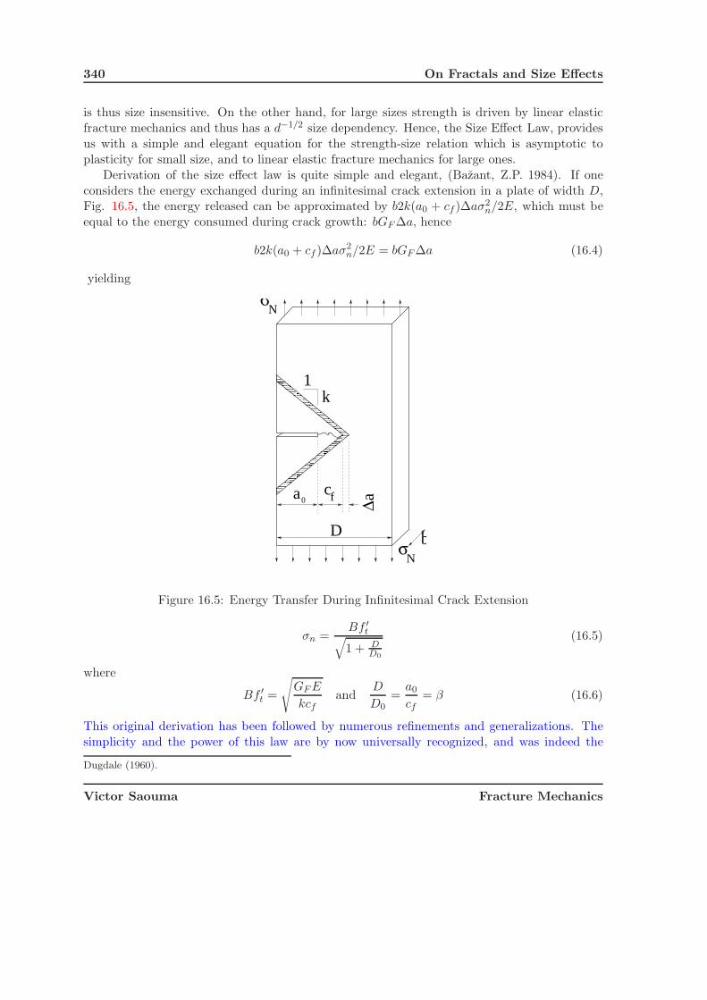
340 On Fractals and Size Effects
is thus size insensitive. On the other hand, for large sizes strength is driven by linear elasticfracture mechanics and thus has a d−1/2 size dependency. Hence, the Size Effect Law, providesus with a simple and elegant equation for the strength-size relation which is asymptotic toplasticity for small size, and to linear elastic fracture mechanics for large ones.
Derivation of the size effect law is quite simple and elegant, (Bazant, Z.P. 1984). If oneconsiders the energy exchanged during an infinitesimal crack extension in a plate of width D,Fig. 16.5, the energy released can be approximated by b2k(a0 + cf )Δaσ2
n/2E, which must beequal to the energy consumed during crack growth: bGF Δa, hence
b2k(a0 + cf )Δaσ2n/2E = bGF Δa (16.4)
yielding
σN
cf aΔ
Dσ
a
N
b
1k
0
Figure 16.5: Energy Transfer During Infinitesimal Crack Extension
σn =Bf ′
t√1 + D
D0
(16.5)
where
Bf ′t =
√GF E
kcfand
D
D0=
a0
cf= β (16.6)
This original derivation has been followed by numerous refinements and generalizations. Thesimplicity and the power of this law are by now universally recognized, and was indeed the
Dugdale (1960).
Victor Saouma Fracture Mechanics

16.1 Introduction 341
subject of Prof. Bazant inaugural article at the National Academy of Sciences, (Bazant, Z.P.2005).
Saouma, Natekar and Hansen (2003) proposed an alternative derivation of only Bazant’soriginal size effect law. Contrarily to the original Lagrangian derivation based in energy transfer,a Newtonian one based on local stress intensity factors was proposed. The stress intensity factorsdue to the far field (constant traction on an infinite plate) and cohesive stresses are:
Ka = σ√
πa (16.7)
Kb = f ′t
√πa
(1 − 2
πarcsin
a − cf
a
)(16.8)
respectively, (Cherepanov 1979). Equating those two stress intensity factors, we obtain thenominal strength
σn = f ′t
[1 − 2
πarcsin
(1 − cf
a
)](16.9)
In the limit, for small sizes when a � cf , σn approaches asymptotically f ′t. On the other hand,
for large sizes, cf � 0, σn will asymptotically approach zero. Whereas the expression of σn
appears to have the same limits as the Size Effect Law, it is not mathematically similar toit. This will only become apparent if one takes a series expansion of the ArcSin function, andsubstituting cf/a by s:
σn = σn = f ′t
[1 − 2
πarcsin(1 − s)
](16.10)
� 2√
2f ′t
πs1/2 +
f ′t
3√
2πs3/2 +
3f ′t
40√
2πs5/2 + O[s]7/2 (16.11)
Neglecting the terms of power greater than 1 (since s is at most equal to 1), and substitutings = 1/(1 + r) where r = a0/cf , we obtain
σn =2√
2
π︸ ︷︷ ︸B
f ′t
√√√√√ 1
1 + r︸︷︷︸β
(16.12)
Interestingly, this equation, Fig. 16.6 was derived on the basis of a simplified fixed cohesivestress profile, and not through the generally accepted fixed stress-displacement law of Hillerborg(similar analytical derivation was given in Sec. 9.4.1 of (Bazant, Z.P. 2002). Furthermore, thisderivation has the advantage of establishing a direct relationship between fracture mechanicsand size effect (though an earlier link, albeit through a radically different approach, was estab-lished by Bazant, Z.P. and Kazemi, M.T. (1990)). Finally, constants B and β are explicitlyderived.
16.1.2.2 Carpinteri
In one of his earliest publications, Carpinteri, Chiaia and Ferro (1995) presented a radicallydifferent model for the scale variation of strength. It was assumed that “the effect of mi-crostructural disorder on mechanical behavior becomes progressively less important for larger
Victor Saouma Fracture Mechanics

342 On Fractals and Size Effects
0.001 0.01 0.1 1 10 100
D�������
D0
0.1
0.15
0.2
0.3
0.5
0.7
1
Σn�������
ft
Figure 16.6: Bazant’s original size effect law
scales, whereas it represents the fundamental feature for smaller scales”. The disorder beingexpressed through a fractality, it is postulated that the fractal dimension approaches the topo-logical one asymptotically with increased observation scale length. At the other extreme, forvery small dimensions, it is postulated that linear elastic fracture mechanics is supposed to gov-ern the collapse mechanism of an unnotched material (‘the Griffith’s mode of collapse governedby 0.5 stress singularity becomes the main failure mechanism”). This purely speculative andqualitative model is called multifractal scaling law (MFSL) and is expressed as, Fig. 16.7.
σu(b) = ft
[1 +
lchb
]1/2
(16.13)
Indeed for “large” dimensions, a constant stress, unburdened by fractals or disorder, is reached.
ln chl
lnσ
12
( )ln t chf lln tf
ln b
1
EuclidianFractal
ln chl
ln FG
2
ln b
ln F
ch
G
l
⎛ ⎞⎜ ⎟⎜ ⎟⎝ ⎠
EuclidianFractal
ln chl
ln cε
1
ln b
0ln cε
EuclidianFractal
1
Tensile Strength Fracture Energy Critical Strain
ln chl
lnσ
12
( )ln t chf lln tf
ln b
1
EuclidianFractal
ln chl
ln FG
2
ln b
ln F
ch
G
l
⎛ ⎞⎜ ⎟⎜ ⎟⎝ ⎠
EuclidianFractal
ln chl
ln cε
1
ln b
0ln cε
EuclidianFractal
1
Tensile Strength Fracture Energy Critical Strain
Figure 16.7: Multifractal Scaling Laws (Carpinteri)
Whereas, for “small” sizes, the bilogarithmic diagram tends to -0.5.This model calls for the following observations:
1. Conceptually it is hard to refer to a stress singularity when there is no crack (for verysmall sizes), and should there be one, we are at a scale where it is well established that (in
Victor Saouma Fracture Mechanics

16.1 Introduction 343
either elasto-plastic metals, or in cementitious material) there are cohesive stresses whichdefeat the applicability of LEFM as was well established by Irwin (1960) (elasto-plasticfracture mechanics), and Hillerborg, A. and Modeer, M. and Petersson, P.E. (1976a)(cohesive crack model). Furthermore, and most surprisingly, this model makes absolutelyno reference to the geometry of the structure where the fractal crack is embedded. Surely,this should have to be accounted for somewhat.
2. Whereas Bazant’s asymptotic analysis, (Bazant, Z.P 1997) yields a non zero strength forlarge sizes Carpinteri’s model can be criticized for not having an upper bound to thestrength as size is reduced. It is well known that the theoretical strength, based on inter-atomic forces, will have to be an upper bound as size is reduced (such as in nano-tubes),(Kelly 1974).
σtheormax =
√Eγ
a0(16.14)
where E, γ and a0 are the elastic modulus, surface energy, and distance separating twoatoms respectively.
3. This model, first based on speculative assumptions (multifractal) is mathematically de-fined by an empirical relationship which happens to satisfactory fit reported experimentaldata (just as the empirical fatigue model of ? and contrarily to the analytically derivedsize effect law of Bazant).
4. There are no indications that this model is restricted to cementitious materials, and thereis no explicit reference to cohesive stresses.
Hence, the mere fact that it adequately fits some experimental data, is of no scientific relevance.The most recent formal derivation of the multifractal model was presented in a recent
(survey) paper, by Carpinteri, Chiaia and Cornetti (2003). Hence transforming a previouslypresented empirical law into a semi-analytical one. This derivation was itself a restatement ofan earlier one by Carpinteri (1994) which was recently shown in the Appendix of (Bazant, Z.P.and Yavari, A. 2005) to be mathematically flawed.
Without going through the details, we note that the fracture energy GF is now shown tobe also size dependant, or more specifically multifractal. Furthermore, the −1/2 exponent,previously attributed to LEFM for small size, is now attributed/justified by Brownian disorderwhich (according to the authors) should correspond to fractal scaling of +1/2 and -1/2 forinvasive (strength) and lacunar (fracture energy) morphologies.
Starting from3
W = GF A0 = G∗F Ao (16.15)
where G∗F is a true scale invariant material parameter, whereas GF is subjected to a scale effect
described by a positive power law, the authors go on in defining:
GF (b) ∼ G∗F bDG (16.16)
3Incidentally, this equation is identical to Eq. 16.3.
Victor Saouma Fracture Mechanics

344 On Fractals and Size Effects
σu(b) ∼ σ∗ub−Dσ (16.17)
εc(b) ∼ ε∗cb1−Dε (16.18)
1 = DG + Dσ + Dε (16.19)
which ultimately yields:
GF (b) = G∞F
[1 +
lchb
]−1/2
(16.20)
wc(b) = w∞c
[1 +
lchb
]−1
(16.21)
where lch is a characteristic length, b a representative dimension. Again, it should be noted thatwhereas in his original publication Carpinteri associates the +1/2 exponent to LEFM, in thismore recent ones, the fractal scaling of +1/2 and -1/2 now correspond to the highest possible(Brownian) disorder. This is at best a convenient (and yet unproven) conjecture as it is not clearwhat exactly is meant by Brownian movement4. Einstein’s work on Brownian movement (inliquid and gas, and not in solids) is at a scale much smaller than the one of Engineering interest.At this scale Newtonian physics is certainly no longer applicable, and should be replaced byQuantum Physics. Hence, it is at best difficult to reconcile physical models at such differentscales without a rigorous explicit justification. To the best of the authors knowledge, no modelspanning those two realms has even been proposed by theoretical physicists.
16.1.3 Historical Notes
It is commonly stated that size effect phenomenon was first highlighted by Galilei (1638), on thebasis of his famous etchings of different sizes of animal bones, Fig. 16.8. Galileo was indeed the
Figure 16.8: The Scaling of Bones, Galilei (1638)
first to notice that smaller objects in nature are not just scaled replicas of similar big objects.In the Dialogues concerning two new sciences, Proposition IX (on the second day), Salviatistates:
4Brownian motion was discovered in the 19th century by R. Brown who observed through a microscope therandom swarming motion of pollen grains in water (now understood to be due to molecular bombardment). Thetheory of Brownian motion was later developed by Einstein (1905) to estimate the size of molecules.
Victor Saouma Fracture Mechanics

16.1 Introduction 345
...I once drew the shape of a bone, lengthened three times, and then thickened insuch proportion that it could function in its large animal relatively as the smallerbone serves the smaller animal: here are the pictures; You see how disproportionatethe shape becomes in the enlarged bone. From this it is manifest that if one wishedto maintain in an enormous giant those proportions of members that exist in anordinary man, it would be necessary to either find much harder and more resistantmaterial to form his bones, or else to allow his robustness to be proportionatelyweaker than in men of average stature; otherwise growing to unreasonable height,he would be seen crushed by his own weight and fallen.
Evidently, Galileo lacked the algebraic notation to do dimensional analysis in the way Vashy(1892) later on introduced it through the fundamental length parameter L. Hence, cast in thecurrent context, Galileo’s statement would simply read as follows: the weight a bone carries isproportional to the animal volume (L3) whereas the strength of this same bone is proportionalto its cross section area L2. A simple dimensional analysis shows that if an animal is, forexample, three times larger, Its bone would be three times longer but should be 33/2 ∼= 5 timeswider in order to carry the weight. This explains why a giant animal cannot have the sameproportions as its smaller model. Hence, again Galileo’s “paternality” of the Size effect lawcan not be attributed to this observation, which again has more to do with mere dimensionalanalysis.
Hence, for a superficial observer (or a modern day Simplicio), Galileo would be the fatherof scaling (or dimensional) theory, and not of size effect theory. However, if we can (with alldue respects) paraphrase Galileo we would simply say that weight increases with L3 and loadcarrying capacity (constant strength, variable cross-section) increases with L2. This is exactlywhat the Size Effect law is all about: energy is released from a volume ∝ L3 and absorbedby a surface crack ∝ L2. As is well known by now, there are many experimental evidencessupporting both Galileo and Bazant, (RILEM TC QFS 2004).
To that far-reaching statement, the incredulous Simplicio states:
But the immense bulks that we encounter among fishes give me grave reason to doubtwhether this is so. From what I hear, a whale is as large as ten elephants; yet whaleshold together.
This questioning by Simplicio is not different than the incredulity of many skeptical moderntime engineers, regarding the Size Effect law. But again, Salviati wisely replies:
Your doubt, Simplicio, enables me to deduce something that I did not mention before,a condition capable of making giants and other vast animals hold together and movearound as well as smaller ones. That would follow if, but not only if, strength wasadded to the bones and other parts whose function is to sustain their own weightand that which rests on them.
Now, Galileo is implying that nominal strength (and not anymore mere load carrying capacity)can increase at times and that strength does not necessarily diminishes with size. In modern
Victor Saouma Fracture Mechanics

346 On Fractals and Size Effects
days terminology, Galileo is stating that strength does not necessarily drop to zero, which is acommon feature of both Carpinteri’s multi-fractal model, and Bazant’s revised size effect law,(Bazant, Z.P. and Novak, D. 2000).
In more recent times, Weibul size effect was early on examined by Griffith (1921) whowas seeking for an explanation of the increased strength with the reduction in glass filamentdiameter. His genius was to explain the strength reduction through the stress concentrationaround an elliptical crack as derived by Inglis (1913), and in postulating the energy transferfrom strain to surface. However, it should be kept in mind that this model is applicable onlyfor perfectly brittle solids, and not for quasi-brittle ones.
Finally, the size effect law provides us with a unified model for small scale plasticity to largescale fracture (linear elastic). In that context, it can be viewed as an analogy to the columncurve which provides for a unified model of strength across a wide spectrum of slenderness ratios.At one end, failure is through yielding, and at the other through instability (Euler buckling).The first semiempirical column formula was developed by the second theory of elastic-plasticbuckling of Engesser (1895) as cited in Bazant and Cedolin (1991).
16.2 Fractal Stress Intensity Factors
Yavari, Sarkani and Moyer (2002) investigated the stress and strain singularity at the tip ofa fractal crack. It was shown that for modes I, the fractal crack stresses have the followingasymptotic distribution
σFij(r, θ) = KF
I r−α(θ,D|H) + higher-order terms (16.22)
For self similar cracks,
α =2 − DF
21 ≤ DF ≤ 2 (16.23)
where Df varies from 1 to 2, the lower bound corresponds to the case of a smooth crack, whilethe upper limit represents an infinitely irregular fractal curve that “fills the plane”, and can beenvisioned as a void contained within the plane. For self-affine cracks,
α =
{2H−12H 1/2 ≤ H ≤ 1
0 0 ≤ H ≤ 1/2Self-affine (16.24)
where H is the Hurst exponent and varies from 0 to 1; however stresses and strains are singularat the crack tip only if 1/2 ≤ H ≤ 1, for very rough cracks (H ≤ 1/2), there is no singularity.Hence a fractal crack has a weaker singularity than an Euclidian one..
16.2.1 Far Field Stress
The stress intensity factor for a fractal crack of length 2a and characterized by a fractal sin-gularity α (or roughness H) in an infinite plate subjected to a uniform far field stress σ was
Victor Saouma Fracture Mechanics

16.2 Fractal Stress Intensity Factors 347
derived by Wnuk and Yavari (2003)(Eq. A14 in which s = x/a) as
KFσ =
σ
παaα−1
1∫0
(1 + s)2α + (1 − s)2α
(1 − s2)αds
︸ ︷︷ ︸χ(α)
(16.25)
For the Euclidian crack, α = 1/2, χ(1/2) = π, and Kσ = σ√
πa.
16.2.2 Cohesive Crack
The cohesive crack model is illustrated by Fig. 16.2.2 where a crack of length 2a has cohesivestresses, applied over cf at the crack tip. Introducing the nondimensional distance
x
tftf
0a
a a
a0
σ
cf
cf
σ
Figure 16.9: Cohesive Stress Distribution Along a Fractal Crack
λ =x − a0
a − a0=
s − m
1 − m(16.26)
Where m = a0/a, Wnuk and Legat (2002) defined a generalized cohesive stress distribution
G(λ, ω, n) = λn exp[ω(1 − λ)] (16.27)
For ω = n = 0, we would have a constant cohesive stress as defined by Dugdale (1960), and forω = 0, n = 1 we recover the linear cohesive stress distribution of Barenblatt (1962), Fig. 16.10.
Victor Saouma Fracture Mechanics

348 On Fractals and Size Effects
0 0.1 0.2 0.3 0.4 0.5 0.6 0.7 0.8 0.9 10
0.5
1
1.5
2
2.5
3
3.5
λ
λn exp
( ω
(1−
λ) )
Dugdale modelBarenblatt modelGeneral function
Figure 16.10: Generalized Cohesive Stress Distribution
Using this representation of the cohesive stress, Wnuk and Yavari (2003) gave an expressionof the non-fractal cohesive stress intensity factor (Eq. 16) which can be rewritten as
Kcoh =2f ′
t
π
√πa
∫ 1
0
G(λ, ω, n)(1 − m)√1 − [(1 − m) λ − m]2
dλ (16.28)
Following an approach similar to the authors, it can be shown that the fractal counterpart ofthis equation is
KFcoh =
2f ′t
π(πa)1−α(1 − m)1−α
∫ 1
0
G(λ, ω, n)
{(1 − λ) [1 + (1 − m)λ + m]}α dλ︸ ︷︷ ︸Γ(ω,n,α,m)
(16.29)
For small scale yielding, m → 1, then the preceding equation simplifies to the one given in Eq.25 by Wnuk and Yavari (2003)
KFcoh =
[2ft
π(πa)1−α
](1 − m)1−α
2α
1∫0
G(λ, ω, n)
(1 − λ)αdλ
︸ ︷︷ ︸Γ(ω,n,α)
(16.30)
which, for an Euclidian crack (α = 1/2), is further simplified to
Kcoh =
[√2ft
π
√πa
]√1 − m · Γ(ω, n,
1
2) (16.31)
Victor Saouma Fracture Mechanics

16.3 Fractal Size Effect 349
16.3 Fractal Size Effect
Following the same approach developed by (Saouma et al. 2003) to rederive (all operationswere performed with the help of Mathematica) the size effect law, we seek to remove the stresssingularity by setting
KFσ + KF
coh = 0 (16.32)
and solving for σ.First we attempt to obtain the generalized fractal size effect law by considering the general
expression of KFcoh (Eq. 16.29) and KF
σ (Eq. 16.25), this yields
σ
f ′t
= −2
(1
1 + r
)1−α Γ(ω, n, α,m)
χ(α)(16.33)
We note that we recover Bazant’s original size effect law for α = 1/2, and that the size effectlaw is clearly independent of the cohesive stress distribution Γ(ω, n, α,m). On the other hand,if we make the assumption of small scale yielding m → 1 we obtain
σ
f ′t
= −21−α(
1
1 + r
)1−α Γ(ω, n, α)
χ(α)(16.34)
Because of its complex form, χ(α) can not be explicitly evaluated, hence, we take a seriesexpansion with respect to s = 0, i.e. for cf � a
χ(α) = 2 + O[s]2 (16.35)
Substituting the first series expansion of χ(α) and the general expression of Γ(ω, n, α,m) fromEq. 16.29 (with G(λ, 0, 0) = 1 for Dugdale’s cohesive stress distribution) into Eq. 16.33 weobtain
σ
ft= −
2−2α(−1 − r)(
11+r
)2α[22α√πΓ(1 − α) − 2B 2r+1
2(r+1)(1 − α, 1 − α)Γ(3/2 − α)
]Γ(3/2 − α)
(16.36)
where
Γ(z) =
∫ ∞
0tz−1e−tdt (16.37)
Br(z,w) =
∫ r
0tz−1(1 − t)w−1dt (16.38)
are the Gamma and Beta functions. Fig. 16.11 shows the size effect law for fractal cracks. Wenote that the strength of a fractal crack is always larger than the one of an Euclidian one. Thisis consistent with Eq. 16.22 derived by Yavari et al. (2002).
The analytical expression of the slope as r → ∞ in terms of α, was derived but wasexceedingly complex and could not be reduced to a simpler expression. However, when thisexpression is plotted, Fig. 16.12 it is exceedingly simple, and it would appear that the slope
Victor Saouma Fracture Mechanics

350 On Fractals and Size Effects
�4�2
02
4
Log�r�0
0.10.2
0.30.4
0.5
Α
�2
�1
0
Log�Σ�ft�
0.10.2
0.30.4
0.
�2
�1
0
Figure 16.11: Fractal Size Effect Laws (Dugdale)
0.1 0.2 0.3 0.4 0.5Α
�0.5
�0.4
�0.3
�0.2
�0.1
Slope as r� �
Figure 16.12: Slope of the Fractal Size Effect Law in terms of α as r → ∞
Victor Saouma Fracture Mechanics

16.4 Cellular Automata 351
is simply equal to α. Indeed the -1/2 asymptotic slope of Bazant’s original size effect law isrecovered, and the strength of the size effect law is reduced for fractal cracks.
Similarly, if we one examine the asymptotic value of σ/f ′t as r → 0, we obtain, Fig. 16.13
σ
ft
∣∣∣∣r−→0
=
√πΓ(1 − α)
2Γ[
32 − α
] (16.39)
which for α = 1/2 is equal to π2 . Evidently, this limit value is problematic, as one would have
0.1 0.2 0.3 0.4 0.5Α
1.1
1.2
1.3
1.4
1.5
Σ�ft as r� 0
Figure 16.13: Asymptotic Values of the Size Effect Law as r → 0
expected to retrieve the value of 1. This discrepancy may be attributed to the approximationof χ(α) in Eq. 16.35; nevertheless this discrepancy requires further investigation.
16.4 Cellular Automata
When Fractals were first introduced in the early 80’s it rapidly spread in multiple disciplinesof science and engineering. To the best of the author’s knowledge, one of the first applicationin engineering was in fracture mechanics, when Mandelbrot et al. (1984) showed that metal-lic fracture surfaces are fractals. This was one key paper which subsequently inspired manyothers, including this one. Similarly, we recently witnessed the development of a “New Kindof Science” by Wolfram (2002). Again, just as Mandlebrot did in 1984, Wolfram asserts thathis Cellular Automata can model the roughness of cracks. Given the inherent similarity be-tween cellular automata and fractals, the authors conclude by examining what may become yetanother fracture representation and its role in fracture mechanics.
Crack models need not only be based on continuum (even if fractal) models, but can bebased on discontinuous ones too. Whereas the lattice model is by now making great stridestoward its acceptability, (Cusatis, Bazant and Cedolin 2003), a new model based on cellularautomata was recently proposed by Wolfram (2002) (A New Kind of Science (NKS)). Thismodel is worth mentioning for two reasons. First it provides a simple algorithm to definecomplex objects, which at time are exact replicas of fractals. Secondly, the author claims thathis rules 150 (shown below), 22, and 122 can be used to model a random crack, which in thecontext of this paper does indeed appear to be fractal.
Victor Saouma Fracture Mechanics

352 On Fractals and Size Effects
Hence, using simple rules, Wolfram’s cellular automata operations can indeed generatefractal objects. In particular, Rule 150 generates a Sierpinski’s like surface, Fig. 16.14 whichbears great resemblance to Fig. 16.2. Rule 150 (Weisstein 2004) is identified by Wolfram (2002)
1 0 101 010
Rule 150
150 10010110= 1 0 101 010
Rule 150
150 10010110=
Figure 16.14: Cellular Automata Definition of Rule 150 Along WIth Potential Crack Path
(pg. 375) as a possible fracture and “at each step, the color of each cell, which roughly representsthe displacement of an element of the solid, is updated according to the cellular automation rule.(The line), representing the location of a crack, moves from one cell to another based on thedisplacements of the neighboring cells, at each step setting the cell it reaches to be white.”.
Hence, whereas fractals constitute a static way to mathematically catalog the points thatmake up the object, cellular automata are a dynamic way to create the object via a growthprocess.
Yet, despite the ability to replicate a fractal surface, which can greatly reassemble a crackedfractal surface, the NKS fails to provide any mathematical or physical parameters which canbe exploited to further investigate the problem beyond a mere graphical representation. Never-theless, it is somehow the intuition of the authors that this model could be further investigatedthrough the prism of the size effect law, and may very well lead to some interesting (albeitqualitative) results.
16.5 Conclusion
Both Bazant’s size effect law (SEL) and Carpinteri’s multifractal scaling law (MFSL) are thor-oughly reviewed. Serious reservations on the second model are cast, while the first one isextended to include fractal cracks. Historical notes pertaining to these models are also dis-cussed. Finally, speculative remarks on the applicability of cellular automata on size effectsand fractals are made.
Victor Saouma Fracture Mechanics

16.5 Conclusion 353
The derived fractal size effect law does account for the geometry of the structure, is con-sistent with Bazant’s original derivation. However, it should be noted that there is still adiscrepancy in the plastic asymptote, and this model does not extend Bazant’s subsequent re-finements of his model. It is shown that as the fractal dimension increases (i.e. α decreasingfrom 1/2), the nominal strength does also increase. In the limiting case of α = 0 (essentially aplate with a hole), then no longer is the strength dependant on the size, i.e plasticity reigns.
Accepting the cohesive crack model, the proposed Fractal Size Effect Law (FSEL) in noways resembles MFSL (which still lacks a rigorous mathematical derivation).
Based on the comprehensive, historical and rigorous discussion presented in this paper, itis hoped that the controversy surrounding the discrepancy between SEL and MFSL is laid torest, and that code writers should have no qualm in embracing Bazant’s Size Effect Law. Para-phrasing (Izquierdo-Encarnacion 2003), we can definitely conclude that Effectus amplitudinisfractae rimae satisfaciendus est. (Fractal cracks must obey Size Effects).
Victor Saouma Fracture Mechanics

354 On Fractals and Size Effects
Victor Saouma Fracture Mechanics

Chapter 17
FRACTURE MECHANICSPROPERTIES OF CONCRETE
Adapted from (Saouma, Broz, Bruhwiler and Boggs 1991)
17.1 Introduction
Concrete dams are often referenced as a potential application of Fracture Mechanics, yet, littlework has been performed to evaluate fracture properties of dam concrete. Most of the researchundertaken on the fracture of concrete has concentrated on laboratory testing of small speci-mens constructed of structural concrete. Based on these test results, a basic understanding ofthe fracture processes occurring in concrete has been developed. However, since the fractureparameters often appear to be size and aggregate dependent, the experimentally determinedvalues cannot be reasonably extrapolated to mass concrete structures such as dams.
The fracture properties obtained from small concrete specimens may be size and geometrydependent because the fracture ligament of the specimens is too short to achieve a steady crackpropagation regime. Several experimental investigations have been performed on large concretemembers to determine both “objective” fracture properties and minimum dimensions for testspecimens. Large scale double cantilever beams with a length of 350-cm (138-in.) have beenused at the “Laboratoire Central des Ponts et Chaussees” in Paris since 1976 (Chhuy et al.1979, Rossi et al. 1984) for fracture testing of concrete. An investigation using four differentspecimen geometries ranging in size from 100-cm (39.4-in.) to 144-cm (56.7-in.) is presentedin Wittmann & Metzener-Gheorghita (1985). Other large concrete fracture specimens includethree–point bend (TPB) beams with a depth of 80-cm (31.5-in) (Hilsdorf & Brameshuber 1985),compact tension (CT) specimens with heights ranging from 30-cm (12-in.) to 150-cm (59-in.)(Wittmann et al. 1988), and tapered double cantilever beams with a height of 210-cm (83-in.)(Rossi et al. 1990).
In this chapter, testing and data evaluation procedures developed for relatively small spec-imens are extended to a series of large concrete Wedge Splitting (WS) specimens with heightsof 31-cm (12-in.), 91-cm (36-in.) and 152-cm (60-in.). Three different concretes with maximum

356 FRACTURE MECHANICS PROPERTIES OF CONCRETE
aggregate sizes, 19-mm (0.75-in.), 38-mm (1.5-in.) and 76-mm (3.0-in.), representative of massconcrete used in dams are examined. A test series of WS specimens used to study the fracturebehavior of the cold–joint between lifts in a dam is also presented. From each set of experi-ments, values for fracture toughness, KIc, and specific fracture energy, GF , are determined anddiscussed. The influence of aggregate shape and geological origin on the fracture properties arealso considered.
17.2 Experiments
17.2.1 Concrete Mix Design and Specimen Preparation
Unlike structural concrete, in which the maximum size aggregate (MSA) typically does notexceed 38-mm (1.5-in.) in diameter, in dam concrete mixes the MSA is, in general, equal to orlarger than 76-mm (3.0-in.) in diameter. Based on the presence of such large aggregates in adam concrete mix, three MSAs were selected for testing: 19-mm (0.75-in.), 38-mm (1.5-in.), and76-mm (3-in.). For each aggregate size, a concrete mix similar to those used in actual gravitydams was obtained from the U.S. Bureau of Reclamation, which is the agency responsible forthe design, construction, and maintenance of many federally owned dams in the western UnitedStates. The majority of the mixes were batched with rounded river aggregates, except for abatch of the 38-mm (1.5-in.) MSA mix, which consisted of quarried subangular aggregates.Details of the mix designs used for the construction of all specimens are shown in Table 17.1.
Ten standard 15-cm (6.0-in.) × 30-cm (12.0-in.) cylinders for the 19-mm and 38-mm MSAmixes, and ten 30-cm (12.0-in.) × 60-cm (24.0-in.) cylinders for the 76-mm mix were used forthe determination of the concrete material properties. The compressive strength, f ′
c, and tensilesplitting strength, f ′
t,sp, of each concrete mix were obtained prior to performing each wedge-splitting (WS) specimen test. The mean values obtained from unconfined compression tests,performed according to ASTM C39 (Anon. 1983), and the splitting tension test (Brazilian)described in ASTM C496-85 (Anon. 1985), are summarized in Table 17.2.
The test specimen shape used for the experimental program was the wedge-splitting geom-etry, shown in Fig. 17.1, which had been previously used in research programs for the testing
Figure 17.1: *Wedge-splitting specimen geometry.
of small concrete specimens (Hillemeier & Hilsdorf 1976, Linsbauer & Tschegg 1986, Bruhwiler1988, Bruhwiler & Wittmann 1990). The WS specimen has a large fracture area compared tothe concrete volume, approximately 4.6 times greater than a commonly used three-point bend(TPB) beam geometry (RILEM 1985) of equal volume. The large fracture area compared to
Victor Saouma Fracture Mechanics

17.2 Experiments 357
Table 17.1: Concrete mix design.
CONCRETE MIX DESIGN(no entrained air, w/c ratio= 0.55)
maximum aggregate size mix
19-mm (0.75-in.) 38-mm (1.5-in.) 76-mm (3.0-in.)Weight Weight Weight
kg/m3(lb/yd3) kg/m3(lb/yd3) kg/m3(lb/yd3)water 163 139 102
(275) (233) (174)cement 297 252 187
(500) (424) (315)sand 918 782 695
(1,550) (1,320) (1,170)19-mm MSA 978 609 491
(0.75-in.) (1,650) (1,030) (827)38-mm MSA 0 609 491
(1.5-in.) (1,030) (827)76-mm MSA 0 0 491
(3.0-in.) (827)
total 2,390 2,420 2,480(4,030) (4,080) (4,180)
Table 17.2: Experimentally obtained material properties of the concrete mixes used.
MSA f ′
c, MPa (psi) f ′
t,sp, MPa(psi) Eeff , MPa (ksi)
19-mm (0.75-in.) 25.6 (3,710) 2.81 (407) 18,000 (2,610)38-mm (1.5-in.) 24.8 (3,600) 2.67 (388) 16,900 (2,460)
38-mm (1.5-in.) sub-angular 36.6 (5,317) 3.96 (574) 23,200 (3,360)76-mm (3.0-in.) 18.9 (2,740) 2.41 (349) 16,500 (2,400)
Victor Saouma Fracture Mechanics

358 FRACTURE MECHANICS PROPERTIES OF CONCRETE
the aggregate size and specimen volume makes the WS geometry well suited for testing largeMSA and specimens under laboratory conditions.
The dimensions of the WS specimens tested in the experimental program are summarized inTable 17.3. The specimen dimensions and aggregate sizes were selected to enable a comparison
Table 17.3: Wedge-splitting specimen dimensions.
Specimen Dimensions, cm (in.)
Specimen Type H w t s D a0 h
“Small” 31 (12.0) 31 (12.0) 23 (9.0) 6 (2.25) 3 (1.0) 4.5(1.75) 20 (8.0)“Medium” 91 (36.0) 91 (36.0) 41 (16.0) 15 (6.0) 8 (3) 15.2 (6.0) 61 (24.0)“Large” 152 (60.0) 152 (60.0) 41 (16.0) 15 (6.0) 8 (3) 30.5 (12.0) 107 (42.0)
with results previously obtained by other researchers in the academic community, and to predictfracture properties of dam concrete with intermediary values to ensure a continuity of results.
Specimen construction consisted of wooden formwork built for the placing of the concrete, asharpened 3.2-mm (0.125-in.) thick steel plate mounted inside each form to obtain the verticalnotch normal to the load line, and two hollow steel sleeves flanking the plate. Two differentready–mix suppliers delivered the concrete. The first provided the 19-mm and 38-mm MSAmixes and the other the 76-mm MSA concrete mix. In all specimens, with the exception of thecold-joint (CJ) specimens, the concrete was placed with the notch in the vertical direction, andcured at room temperature in the laboratory for at least 28 days prior to testing.
For the CJ specimens, the concrete was placed in two separate lifts, with the notch plateinitially in a horizontal orientation. The tendency of the crack to propagate into the cold-joint,which is a region of inherent weakness, was studied through a slight offset between the initialnotch and the level of the concrete in the first lift. Three days after the first lift was placed, thesurface was sand-blasted to remove surface laitance and ensure a good bond along the joint.Grade 16 silica sand, driven by an air pressure of 100 psi, was used in the blasting process.After sandblasting, the surface was continuously water cured but was saturated surface dry(SSD) when the second lift was placed. The sand-blasting operation and the placing of thesecond lift were performed on the same day. The 38-mm and 76-mm MSA concrete mixes usedfor the CJ specimens were identical to the mix designs used during the standard WS testingprogram. After curing for 28 days, the specimens were turned upright, such that the notch wasin a vertical orientation, and tested using a procedure identical to the standard WS specimensexperiments without the cold-joint. The concrete mixes associated with each specimen size andthe number of specimens in each series are presented in the test matrix of Table 17.4.
17.2.2 Loading Fixtures
For testing, the WS specimens were centered on a steel rod, shown in Fig. 17.2, which acts asa line support along the bottom face of the specimen. The line support fixture was mountedto the actuator of a closed-loop servo-hydraulic materials testing system. Two steel rods were
Victor Saouma Fracture Mechanics

17.2 Experiments 359
Table 17.4: Test matrix.
Number of Tests
Specimen Type Aggregate maximum aggregate size mix
Shape 19-mm (0.75-in.) 38-mm (1.5-in.) 76-mm (3.0-in.)
“Small” rounded 3 3 -“Medium” rounded 3 3 3“Large” rounded - 3 3“Medium” subangular - 3 -“Large” (cold-joint) rounded - 3 3
Figure 17.2: *Wedge fixture and line support.
inserted through steel sleeves in the specimen, and needle bearing rings were mounted on theprotruding ends. The wedge-loading apparatus, also shown in Fig. 17.2, was then fixed andthe WS specimen was raised by the actuator such that the wedges were forced between thebearing rings on each side, imposing a horizontal displacement on the specimen at the point ofcontact. A flexible connection between the wedge-loading fixture and the testing machine loadcell was used to account for any small misalignments and evenly distribute the induced load.As a result of the horizontal displacement imposed by the wedges, the specimen was subjectedto a pure Mode I loading condition.
17.2.3 Testing Procedure
The experimental setup of the electronic controller, the data acquisition system, and the testingmachine for the WS specimen tests are shown in a simplified block diagram in Fig. 17.3. In the
Figure 17.3: *Block diagram of the experimental system.
WS specimen experiments, the primary deformation monitored was the crack–mouth openingdisplacement (CMOD). The CMOD was measured on the top surface of the specimen by a clip
Victor Saouma Fracture Mechanics
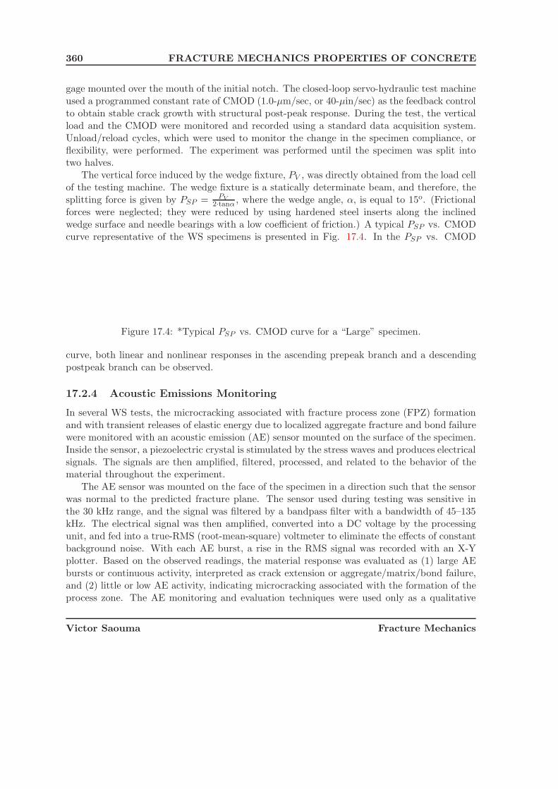
360 FRACTURE MECHANICS PROPERTIES OF CONCRETE
gage mounted over the mouth of the initial notch. The closed-loop servo-hydraulic test machineused a programmed constant rate of CMOD (1.0-μm/sec, or 40-μin/sec) as the feedback controlto obtain stable crack growth with structural post-peak response. During the test, the verticalload and the CMOD were monitored and recorded using a standard data acquisition system.Unload/reload cycles, which were used to monitor the change in the specimen compliance, orflexibility, were performed. The experiment was performed until the specimen was split intotwo halves.
The vertical force induced by the wedge fixture, PV , was directly obtained from the load cellof the testing machine. The wedge fixture is a statically determinate beam, and therefore, thesplitting force is given by PSP = PV
2·tanα , where the wedge angle, α, is equal to 15o. (Frictionalforces were neglected; they were reduced by using hardened steel inserts along the inclinedwedge surface and needle bearings with a low coefficient of friction.) A typical PSP vs. CMODcurve representative of the WS specimens is presented in Fig. 17.4. In the PSP vs. CMOD
Figure 17.4: *Typical PSP vs. CMOD curve for a “Large” specimen.
curve, both linear and nonlinear responses in the ascending prepeak branch and a descendingpostpeak branch can be observed.
17.2.4 Acoustic Emissions Monitoring
In several WS tests, the microcracking associated with fracture process zone (FPZ) formationand with transient releases of elastic energy due to localized aggregate fracture and bond failurewere monitored with an acoustic emission (AE) sensor mounted on the surface of the specimen.Inside the sensor, a piezoelectric crystal is stimulated by the stress waves and produces electricalsignals. The signals are then amplified, filtered, processed, and related to the behavior of thematerial throughout the experiment.
The AE sensor was mounted on the face of the specimen in a direction such that the sensorwas normal to the predicted fracture plane. The sensor used during testing was sensitive inthe 30 kHz range, and the signal was filtered by a bandpass filter with a bandwidth of 45–135kHz. The electrical signal was then amplified, converted into a DC voltage by the processingunit, and fed into a true-RMS (root-mean-square) voltmeter to eliminate the effects of constantbackground noise. With each AE burst, a rise in the RMS signal was recorded with an X-Yplotter. Based on the observed readings, the material response was evaluated as (1) large AEbursts or continuous activity, interpreted as crack extension or aggregate/matrix/bond failure,and (2) little or low AE activity, indicating microcracking associated with the formation of theprocess zone. The AE monitoring and evaluation techniques were used only as a qualitative
Victor Saouma Fracture Mechanics

17.2 Experiments 361
aid to the test.A typical record of the AE-RMS voltage signal for each corresponding load step vs. testing
time is shown in Fig 17.5. The data shown in the curve can be divided essentially into three
Figure 17.5: *Typical AE record for a “Large” WS specimen test.
sections:
Section I: The specimen is in the ascending branch of the PSP vs. CMOD curve, the observedlow AE activity and lift-off of the RMS signal from a baseline value indicates microcrackingand the formation of the process zone at the notch tip.
Section II: The peak load is reached and large AE spikes resulting from crack extension canbe observed.
Section III: The AE bursts increase in amplitude and number, indicating continuous crackformation and growth during the descending branch.
The Kaiser Effect which is characterized by the absence of detectable acoustic emissions untilpreviously applied stress levels are exceeded, is observed in AE testing of composite materials.This effect occurs primarily in the low CMOD regime, and is not visible in Section III. Thelack of the Kaiser Effect in Section III during the unload/reload cycles may have been causedby crushed small concrete particles, and improper fit of the specimen halves. Further applica-tions of this nondestructive evaluation method were performed in the field testing program aspresented in Saouma et al. (1990).
17.2.5 Evaluation of Fracture Toughness by the Compliance Method
The fracture toughness, KIc, was determined using the compliance method. A finite elementcalibration analysis was first performed to determine a relationship between crack length andcompliance, a = a(C), and for the stress intensity factor, KI in terms of crack length:
KI =PSP
H · t√
πaeff · f(β) (17.1)
where β =aeff
H and f(β) is the geometry function for the WS specimens (Saouma et al. 1989a,Broz 1989). In the analysis, both the splitting load and Young’s Modulus E were taken asunity, vertical load components induced by the wedge fixture on the specimen were included,and singular elements were used for SIF determination.
The following general procedure was then followed to interpret the experimental data:
Victor Saouma Fracture Mechanics

362 FRACTURE MECHANICS PROPERTIES OF CONCRETE
1. From the initial ascending branch of the PSP vs. CMOD record, determine the experimen-tal initial specimen compliance Ci
exp, and compare with the normalized (numerical) com-pliance Cn corresponding to a0. From those two values, determine the effective Young’sModulus Eeff = Cn
Ciexp
(Fig. 17.4).
2. For each successive post-peak unload/reload cycle:
(a) Determine the experimental compliance, Ciexp, as the slope of the line obtained by
connecting the initial unloading point to the final reloading point of each cycle (Fig.17.4).
(b) Normalize Ciexp with respect to Eeff and then determine aeff .
(c) From aeff and the Pcr corresponding to the unload point, determine the fracturetoughness, KIc, from Eq. 17.1.
17.3 Fracture Toughness Results
Reduction of the experimental data resulted in a KIc vs. aeff curve that typically exhibitedthree stages (Fig. 17.6). In Stage I, pre-peak unload/reload cycles are performed, and the
Figure 17.6: *The three stages of the fracture toughness vs. effective crack length curve.
section of the curve is included for reference only. Since this stage corresponds to the formationof the FPZ, the stress intensity factor, KI , values increase monotonically up to a plateau. StageII is obtained from the post peak data falling within a plateau. The plateau is synonymous withsteady crack propagation and was also observed by Rossi et al. (1990). Stage III demonstratesa sudden decrease in the KIc values. A possible explanation for this phenomena is based onthe inherent assumptions of the data reduction method. A perfectly linear elastic system wasassumed in the finite element calibration (resulting in zero residual CMOD upon unloading),but the assumption was increasingly violated as the test progressed. As the effective cracklength increased, larger residual CMOD (caused by the inability of the crack to perfectly close)was observed. This effect, at first negligible, eventually becomes predominant as the crack grewdown the ligament.
Only the fracture toughness values associated with Stage II were considered in the statisticalanalysis. The mean values with the respective relative standard deviations are plotted in Fig.17.7 and summarized in Tables 17.5 and 17.6. From the analysis of the experimental datathe following observations are made:
Victor Saouma Fracture Mechanics

17.3 Fracture Toughness Results 363
Figure 17.7: *Mean fracture toughness values obtained from the rounded MSA WS specimentests.
Table 17.5: Summary of fracture toughness data obtained from the WS tests.
Fracture Toughness, KIc, MN/m3/2 (psi√
in)Type 19-mm (0.75-in.) 38-mm (1.5-in.) 76-mm (3.0-in.) Summary
“Small” Mean 1.05 (953) 0.86 (783) - 0.93 (843)rel. σ (%) 5.9 13.4 - 13.9
“Medium” Mean 1.01 (923) 0.99 (909) 1.09 (991) 1.03 (941)rel. σ (%) 20.3 12.7 15.1 16.0
“Large” Mean - 1.23 (1,120) 0.98 (893) 1.16 (1,060)rel. σ (%) - 6.3 12.7 12.8
Summary Mean 1.03 (941) 1.02 (929) 1.05 (957) 1.03 (941)rel. σ (%) 13.5 16.9 15.3 15.2
“Medium” Mean - 1.34 (1,220) - -(subangular) rel. σ (%) - 12.3 - -
Table 17.6: Fracture toughness values obtained from the CJ-WS specimens.
Fracture Toughness, KIc, MN/m3/2 (psi√
in)specimen no.
MSA A B C38-mm Mean 0.64 (582) 0.50 (457) 0.72 (656)(1.5-in.) rel. σ (%) 9.8 3.3 12.1
76-mm Mean 0.71 (643) 0.52 (476) 0.62 (567)(3.0-in.) rel. σ (%) 4.0 2.2 2.7
Victor Saouma Fracture Mechanics

364 FRACTURE MECHANICS PROPERTIES OF CONCRETE
1. Since the relative standard deviations in the vertical columns of Table 17.5 are all within20%, “objective” values, i.e. independent of specimen size, for the fracture toughnesswere determined.
2. Based on the relative standard deviation of the horizontal rows, the fracture toughnessvalues also appear to be independent of aggregate sizes.
3. The previous observation was further evaluated through a test series of medium-size spec-imens constructed with subangular andesite aggregates (as opposed to the rounded ag-gregates used in all previous specimens). The trends in the results of the test series canbe summarized as follows:
(a) The experiments yielded a fracture toughness value of 1.34 MN/m3/2 (1,220 psi√
in),which is 30% higher than the value obtained from the rounded aggregate specimens.
(b) Aggregate debonding was prevalent in fracture surface of the rounded specimens,however, aggregate failures were more predominant in the subangular specimens.
(c) At peak load, the effective crack length of the subangular MSA specimens was foundto be smaller than the aeff of the rounded MSA specimens, indicating the presenceof a smaller process zone.
4. The CJ specimens, which were used to quantify the response of lift-joints found in dams,had:
(a) Peak loads 50% lower than comparable specimens constructed with no “lift” joint.
(b) Fracture toughness values approximately 30-60% lower than for specimens withoutlift joints.
(c) Smaller residual crack opening displacements following each cycle of unload/reload,and no descending portions of the fracture toughness curve (as illustrated in Fig.17.6).
5. A fractal analysis (Gamal-El-Din et al. 1990) of the concrete surfaces yielded a constantfractal dimension for all the rounded aggregate specimens. In the analysis of CJ frac-ture surfaces, a relationship between the fractal dimension and fracture toughness wasobserved.
6. The experiments reported here were conducted in the laboratory environment under un-confined conditions, the effects of confining stresses on the apparent fracture toughnessare presented in Saouma et al. (1990).
17.4 Specific Fracture Energy Results
The specific fracture energy, GF , is defined as the total energy required to break a specimeninto halves, normalized by the projected fracture area. GF is ideally obtained from the area
Victor Saouma Fracture Mechanics

17.4 Specific Fracture Energy Results 365
underneath the load-deformation curve in a direct tension test. Alternatively, specific fractureenergy can also be obtained directly from flexural-based specimen geometries, such as the WSspecimen. In the WS specimens, GF was calculated as the area under the curve of PSP vs.corresponding CMOD, divided by the ligament area (Bruhwiler 1988, Bruhwiler & Wittmann1990). Thus, each test specimen yields one single value of GF . The GF values determined fromthe experiments are shown Tables 17.7 and 17.8 and plotted in Fig. 17.8. Based on the
Figure 17.8: *Mean specific fracture energy values obtained from the rounded MSA WS speci-men tests.
Table 17.7: Summary of specific fracture energy values obtained from the WS tests.
Specific Fracture Energy, GF , N/m(kip/in)Type 19-mm (0.75-in.) 38-mm (1.5-in.) 76-mm (3.0-in.) Summary
“Small” Mean 206 (1.18 × 10⁻³) 238 (1.36 × 10⁻³) - 226 (1.29 × 10⁻³)rel. σ (%) 9.0 11.2 - 12.2
“Medium” Mean 173 (9.88 × 10⁻⁴) 223 (1.27 × 10⁻³) 226 (1.29 × 10⁻³) 211 (1.21 × 10⁻³)rel. σ (%) 29.1 7.5 15.1 15.5
“Large” Mean - 259 (1.48 × 10⁻³) 237 (1.35 × 10⁻³) 254 (1.45 × 10⁻³)rel. σ (%) - 18.1 - 15.7
Summary Mean 189 (1.08 × 10⁻³) 240 (1.37 × 10⁻³) 230 (1.31 × 10⁻³) 226 (1.29 × 10⁻³)rel. σ (%) 19.1 13.5 6.5 15.7
“Medium” Mean - 277 (1.58 × 10⁻³) - -(subangular) rel. σ (%) - 13.8 - -
analysis of the experimental results the following comments can be made:
1. The 38-mm and 76-mm rounded MSA specimens yielded approximately equal values ofGF , which are 10-20 % higher than the values obtained for the 19-mm MSA concrete mix.
2. A similar size dependency for GF for relatively small specimens with ligament lengths ofless than 20-cm was observed by Rossi et al. (1990).
3. The experiments performed on the specimens constructed with the subangular aggregatemix indicated:
Victor Saouma Fracture Mechanics

366 FRACTURE MECHANICS PROPERTIES OF CONCRETE
Table 17.8: Fracture energy values obtained from the CJ-WS specimens.
Specific Fracture Energy, GF , N/m(kip/in)specimen no.
MSA A B C38-mm 99.7 80.6 138.4(1.5-in.) (5.70 × 10⁻⁴) (4.55 × 10⁻⁴) (7.85 × 10⁻⁴)
76-mm 133.0 85.8 98.1(3.0-in.) (7.59 × 10⁻⁴) (4.90 × 10⁻⁴) (5.60 × 10⁻⁴)
(a) GF values were 25% higher than the values obtained from the specimens constructedfrom the rounded aggregate mixes.
(b) The subangular aggregate shape inhibitted debonding, and more energy was requiredto break the sub-angular aggregate than to debond rounded aggregate.
4. For the cold-joint specimens:
(a) The GF values were approximately 40-70 % lower than the standard WS specimens.The lower fracture energy values were attributed to the inherent weakness of thecold-joint between specimen halves.
(b) The higher GF values were correlated to visibly rougher surfaces at the cold-joint.
17.5 Conclusions
1. Based on the concrete mixes tested, which were obtained from two separate local ready-mix suppliers, and using the compliance method for fracture toughness evaluation, theunconfined KIc of concrete is a material constant, equal to 1.04 MN/m3/2 (941 psi
√in).
2. The evaluated fracture parameters, KIc and GF , are independent of specimen size andare “objective” only if certain minimum dimensions are exceeded.
3. The fracture parameters, KIc and GF , are practically independent of aggregate size anddepend on the angularity, or shape, as well as, the aggregate’s strength.
4. For the two types of aggregates used in this experimental program, more energy wasrequired to fracture the subangular aggregates than to debond the rounded ones.
5. Debonding of rounded aggregates may result in a FPZ which is larger than the processzone caused by the fracture of subangular aggregates.
6. The fracture properties for CJ-WS specimens exhibited higher variations in results, andwere lower than for specimens without cold-joints.
Victor Saouma Fracture Mechanics

17.6 Size Effect Law Assessment 367
Table 17.9: Size Effect Law model assessment from the WS test program (averagevalues)(Bruhwiler, E., Broz, J.J., and Saouma, V.E., 1991)
Specimen Size d da a0 a0/d F maxsp σN
mm mm mm kN MPa(in.) (in.) (in.) (kip) (psi)
“Small” 248 19 44.45 0.18 24.1 3.05“Small” 248 38 17.5 2.21
“Medium” 762 19 152.4 0.20 64.0 1.68“Medium” 762 38 69.1 1.81“Medium” 762 76 63.1 1.65“Large” 1,372 38 304.8 0.22 123.9 1.68“Large” 1,372 76 113.5 1.54
17.6 Size Effect Law Assessment
More specifically, an assessment of the size effect law in terms of: 1) testing three concretemixes (with different aggregate sizes) in identical specimen sizes; 2) The same concrete mix onthree different specimen sizes; and finally 3) determination of the fracture toughness throughan extrapolation of the size effect law, (Bruhwiler, E., Broz, J.J., and Saouma, V.E., 1991).
In its original formulation, the Size Effect Law assumes avariation of the nominal strengthin terms of the maximum aggregate size. To assess this dependency, the test data for specimensof “Medium” size, but different da, were analyzed. From Table 17.9 it appeared that aggregatesize does not play a dominant role in assessing the nominal strength of a concrete structure.However, we determined that the shape and geological composition of the aggregates are farmore important parameters.
Alternatively, when geometrically similar specimens with identical concrete mix were con-sidered then indeed the size effect law proved to be a valid tool to determine structure’s nominalstrength, Fig. 17.9.
Finally, the Size Effect Law can be re-arranged in a formulation to predict the fracturetoughness KSEL
Ic , from “small” laboratory test values of a geometrically identical “infinitlylarge” one. It can be shown, (Bruhwiler, E., Broz, J.J., and Saouma, V.E., 1991) that asd → ∞ KSEL
Ic = Y Bf ′t
√d0
Using this equation, the fracture toughness for the WS specimens for d0 = 1570 mm isfound to be KSEL
Ic = 1.54 MN/m3/2 (1.40 ksi√
in), which is 51% higher than the value of KCMIc
= 1.02 MN/m3/2 (0.93 ksi√
in) obtained using the compliance method (CM) (Saouma, Broz,Bruhwiler and Boggs 1991). The difference between KSEL
Ic and KCMIc appears to be large a
priori however it can be explained by the two different approaches used to evaluate fracturetoughness from experimental data. Also, the SEL covers a range of sizes of about 1:20, andtherefore, extrapolation to infinite size may not be valid.
17.7 Notation and Abbreviations
a Crack Length
Victor Saouma Fracture Mechanics

368 FRACTURE MECHANICS PROPERTIES OF CONCRETE
Figure 17.9: Size effect for WS specimens for da=38 mm (1.5 in) (Bruhwiler, E., Broz, J.J.,and Saouma, V.E., 1991)
a0 Initial Notch Lengthaeff Effective Crack LengthCexpi
Initial Experimental ComplianceCexp Experimental ComplianceCn Normalized ComplianceD Diameter of Loading RodsE Young’s ModulusEeff Effective Young’s Modulusf ′
c Concrete Compressive Strengthf ′
t Concrete Uniaxial Tensile Strengthf ′
t,sp Concrete Splitting Tensile Strength
GF Specific Fracture EnergyH Specimen Heighth Specimen Ligament LengthKI Stress Intensity FactorKIc Fracture Toughness (Critical Stress Intensity Factor)KAPP
Ic Apparent Fracture ToughnessPV Vertical ForcePCR Splitting Force Corresponding to Unload/reload CyclePSP Splitting Forces Distance from Top of Specimen to Point of Load Applicationt Specimen Thicknessw Specimen Width
Victor Saouma Fracture Mechanics

17.7 Notation and Abbreviations 369
AE Acoustic EmissionASTM American Society of Materials TestingCJ Cold-JointCMOD Crack Mouth Opening DisplacementCT Compact TensionFPZ Fracture Process ZoneLEFM Linear Elastic Fracture MechanicsLVDT Linear Variable Differential TransformerMSA Maximum Aggregate SizeNLFM Non-Linear Fracture MechanicsRMS Root Mean SquareSOM Strength of MaterialsSSD Saturated Surface DryTPB Three Point BendingWS Wedge Splitting
Victor Saouma Fracture Mechanics

370 FRACTURE MECHANICS PROPERTIES OF CONCRETE
Victor Saouma Fracture Mechanics

Part V
FINITE ELEMENT TECHNIQUESIN FRACTURE MECHANICS


Chapter 18
SINGULAR ELEMENT
18.1 Introduction
1 For most practical problems, either there is no analytical solution, or the handbook ((Tadaet al. 1973)) ones are only crude approximation. Hence numerical techniques should be used.Whereas Boundary Element Methods are increasingly being used, (Aliabadi and Rooke 1991),they are far behind in sophistication the Finite Element Methods which will be exclusivelycovered in this chapter. For an overview of early finite element techniques in finite elements thereader should consult (Owen and Fawkes 1983), some of the more recent methods are partiallycovered in (Anderson 1995). Finally, the Ph.D. thesis of Reich (1993) and of ? contain someof the major extensions of modern techniques to include thermal load, body forces, surfacetractions in 2D and 3D respectively.
2 Numerical methods for fracture mechanics can be categorized in many different ways, in thischapter we shall use three criteria:
1. Those in which the singularity is modelled, that is the r−12 stress field at the tip of the
crack is properly represented.
2. Techniques in which the SIF are directly evaluated as part of the augmented global stiffnessmatrix.
3. Techniques through which the SIF can be computed a post priori following a standardfinite element analysis via a special purpose post-processor.
18.2 Displacement Extrapolation
3 This technique was the predominant one prior to the serendipitous discovery of the quarterpoint singular element.

374 SINGULAR ELEMENT
4 In early finite element studies of LEFM, it was recognized that unless singular elements couldbe used, it would necessitate to have a very fine mesh at the crack tip to approximate the stresssingularity with non-singular elements.
5 Following a liner elastic analysis, the stress intensity factors were determined by equating thenumerically obtained displacements with their analytical expression in terms of the SIF. Sucha correlation will be performed along a radial line emanating from the crack tip, and then thefollowing equations would be used:
4G
√2π
r
{uv
}= KI
{(2κ − 1) cos θ
2 − cos 3θ2
(2κ + 1) sin θ2 + sin 3θ
2
}
4G√
2πr
{uv
}= KII
{−(2κ + 3) sin θ
2 − sin 3θ2
(2κ − 3) cos θ2 + cos 3θ
2
} (18.1)
6 After the SIF would have been determined for each point, they would be plotted with respectto their distance from the crack tip, and the predicted SIF values should be the one extrapolatedfrom the crack tip, Fig. 18.1
Figure 18.1: Stress Intensity Factor Using Extrapolation Technique
7 Usually, θ is taken to be equal to π. A similar approach could be used using stresses ratherthan displacements. However this is likely to yield less accurate predictions.
18.3 Quarter Point Singular Elements
8 This section discusses the easiest and most powerful technique used in finite elements to modela stress singularity.
Victor Saouma Fracture Mechanics

18.4 Review of Isoparametric Finite Elements 375
9 Barsoum (1974) and Henshell and Shaw (1975) independently demonstrated that the inversesquare root singularity characteristic of linear elastic fracture mechanics can be obtained in the2D 8-noded isoparametric element (Q8) when the mid-side nodes near the crack tip are placedat the quarter point.
10 Thus, in order to model a stress singularity without altering the finite element code, themid-side nodes adjacent to the crack tip must be shifted to their quarter-point position. Sincethen this element became known as the quarter-point element.
11 In light of the simplicity and accuracy achieved by this element, this section will:
1. cover a brief review of the isoparametric element formulation
2. show how the element can be distorted in order to achieve a stress singularity
3. determine the order of the stress singularity
4. provide a brief review of all the historical developments surrounding this element
5. discuss the effect on numerical accuracy of element size, order of integration, and localmeshing around the crack tip
6. briefly mention references to other singular elements
18.4 Review of Isoparametric Finite Elements
12 In the isoparametric finite element representation, both the internal displacement and coor-dinates are related to their nodal values through the shape functions:
1 2
34
5
6
7
8
1 2
34
5
6
7
8
x,u
y,v
ξ
η
1
1
1 1
Figure 18.2: Isoparametric Quadratic Finite Element: Global and Parent Element
Victor Saouma Fracture Mechanics

376 SINGULAR ELEMENT
{xy
}=
8∑i=1
[Ni 00 Ni
]{xi
yi
}(18.2)
{d} =
{uv
}=
8∑i=1
[Ni 00 Ni
]{ui
vi
}(18.3)
where the Ni are the assumed shape functions.
13 The shape functions are obtained by mere inspection (i.e. serependitiously),
Ni = 14 (1 + ξξi) (1 + ηηi) (ξξi + ηηi − 1) i = 1, 2, 3, 4
Ni = 12
(1 − ξ2
)(1 + ηηi) i = 5, 7
Ni = 12 (1 + ξξi)
(1 + η2
)i = 6, 8
(18.4)
and are tabulated in Table 18.1.
i Ni Ni,ξ Ni,η
1 14(1 − ξ)(1 − η)(−ξ − η − 1) 1
4(2ξ + η)(1 − η) 14(1 − ξ)(2η + ξ)
2 14(1 + ξ)(1 − η)(ξ − η − 1) 1
4(2ξ − η)(1 − η) 14(1 + ξ)(2η − ξ)
3 14(1 + ξ)(1 + η)(ξ + η − 1) 1
4(2ξ + η)(1 + η) 14(1 + ξ)(2η + ξ)
4 14(1 − ξ)(1 + η)(−ξ − η − 1) 1
4(2ξ − η)(1 + η) 14(1 − ξ)(2η − ξ)
5 12(1 − ξ2)(1 − η) −ξ(1 − η) −1
2(1 − ξ2)6 1
2(1 + ξ)(1 − η2) 12(1 − η2) −(1 + ξ)η
7 12(1 − ξ2)(1 + η) −ξ(1 + η) 1
2(1 − ξ2)8 1
2(1 − ξ)(1 − η2) −12(1 − η2) −(1 − ξ)η
Table 18.1: Shape Functions, and Natural Derivatives for Q8 Element
14 As the strain is the derivative of the displacement, we will need later to define ∂N∂x and ∂N
∂y .N has been defined in Eq. ?? - ?? in terms of the natural coordinates ξ and η. Thus the chainrule will have to be invoked and the inverse of the jacobian will be needed.
15 In this case, the jacobian matrix is:
[J ] =
[∂x∂ξ
∂y∂ξ
∂x∂η
∂y∂η
](18.5)
=
[ ∑8i=1
∂Ni
∂ξ xi∑8
i=1∂Ni
∂ξ yi∑8i=1
∂Ni
∂η xi∑8
i=1∂Ni
∂η yi
](18.6)
Victor Saouma Fracture Mechanics

18.5 How to Distort the Element to Model the Singularity 377
16 The inverse jacobian is then evaluated from:
[J ]−1 =
[∂ξ∂x
∂η∂x
∂ξ∂y
∂η∂y
](18.7)
=1
DetJ
[∂y∂η −∂y
∂ξ
−∂x∂η
∂x∂ξ
](18.8)
17 The strain displacement relationship is:
{ε} =8∑
i=1
[Bi][di
](18.9)
where [Bi] is the strain matrix given by:
[Bi] =
⎡⎢⎣
∂Ni
∂x 0
0 ∂Ni
∂y∂Ni
∂y∂Ni
∂x
⎤⎥⎦ (18.10)
where the following chain rule is invoked to determine the coefficients of [B]:⎧⎪⎨⎪⎩
∂N∂x
∂N∂y
⎫⎪⎬⎪⎭ = [J ]−1
⎧⎪⎨⎪⎩
∂N∂ξ
∂N∂η
⎫⎪⎬⎪⎭ (18.11)
18 Finally, it can be shown that the element stiffness matrix of an element is given by (Gallagher1975), (Zienkiewicz 1967):
[K] =
∫ 1
−1
∫ 1
−1[B (ξ, η)] [D] [B (ξ, η)] detJdξdη (18.12)
where the natural coordinates ξ and η are shown in Fig. 18.2 and [D] is the stress-strain orconstitutive matrix.
19 The stress is given by:
{σ} = [D] [B]
{ui
vi
}(18.13)
18.5 How to Distort the Element to Model the Singularity
20 In Eq. 18.13, if the stresses are to be singular, then [B] has to be singular as the two othercomponents are constants. Consequently, if [B] is to be singular then the determinant of Jmust vanish to zero (Eq. 18.5) at the crack tip.
Victor Saouma Fracture Mechanics

378 SINGULAR ELEMENT
21 Now considering a rectangular element of length L along its first side (1-5-2, in Fig. 18.2),we can readily see that both off-diagonal terms (∂y
∂ξ and ∂x∂η ) in J (Eq. 18.5) are zero. Thus, for
the determinant of the jacobian to be zero we must have either one of the diagonal terms equalto zero.
22 It will suffice to force ∂x∂ξ to be zero. Making the proper substitution for ∂x
∂ξ at η = −1 wehave:
∂x
∂ξ
∣∣∣∣η=−1
=8∑
i=1
∂Ni
∂ξxi
=1
4[−1 + 2ξ + 2ξ − 1] (0)
+1
4[1 + 2ξ + 2ξ + 1] (L)
+1
4[−1 + 2ξ − 2ξ + 1] (L)
+1
4[1 − 2ξ + 2ξ − 1] (0)
−2ξ (x5)
+1
2(1 − 1)L
+1
2(1 − 1) (L)
+1
2(1 − 1)
(L
2
)
=1
4(2 + 4ξ) L − 2ξx5 (18.14)
23 After simplification, and considering the first corner node (where η = ξ = −1), we wouldhave:
∂x
∂ξ
∣∣∣∣ ξ=−1η=−1
= 0 ⇔ (1 − 2)L
2+ 2x5 = 0 (18.15)
x5 =L
4(18.16)
24 Thus all the terms in the jacobian vanish if and only if the second node is located at L4 instead
of L2 , and subsequently both the stresses and strains at the first node will become singular.
25 Thus singularity at the crack tip is achieved by shifting the mid-side node to its quarter-pointposition, see Fig. 18.3.
26 We should observe that instead of enforcing ∂x∂ξ along edge 1-2 to vanish at the crack tip, we
could have enforced ∂y∂η along edge 1-7 to be zero at the crack tip.
Victor Saouma Fracture Mechanics
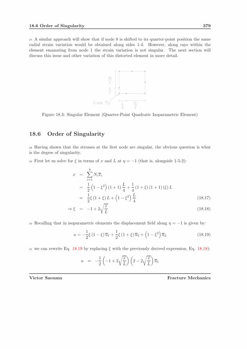
18.6 Order of Singularity 379
27 A similar approach will show that if node 8 is shifted to its quarter-point position the sameradial strain variation would be obtained along sides 1-4. However, along rays within theelement emanating from node 1 the strain variation is not singular. The next section willdiscuss this issue and other variation of this distorted element in more detail.
Figure 18.3: Singular Element (Quarter-Point Quadratic Isoparametric Element)
18.6 Order of Singularity
28 Having shown that the stresses at the first node are singular, the obvious question is whatis the degree of singularity.
29 First let us solve for ξ in terms of x and L at η = −1 (that is, alongside 1-5-2):
x =8∑
i=1
Nixi
=1
2
(1 − ξ2
)(1 + 1)
L
4+
1
4(1 + ξ) (1 + 1) (ξ) L
=1
2ξ (1 + ξ)L +
(1 − ξ2
) L
4(18.17)
⇒ ξ = −1 + 2
√x
L(18.18)
30 Recalling that in isoparametric elements the displacement field along η = −1 is given by:
u = −1
2ξ (1 − ξ) u1 +
1
2ξ (1 + ξ)u5 +
(1 − ξ2
)u2 (18.19)
31 we can rewrite Eq. 18.19 by replacing ξ with the previously derived expression, Eq. 18.18):
u = −1
2
(−1 + 2
√x
L
)(2 − 2
√x
L
)u1
Victor Saouma Fracture Mechanics
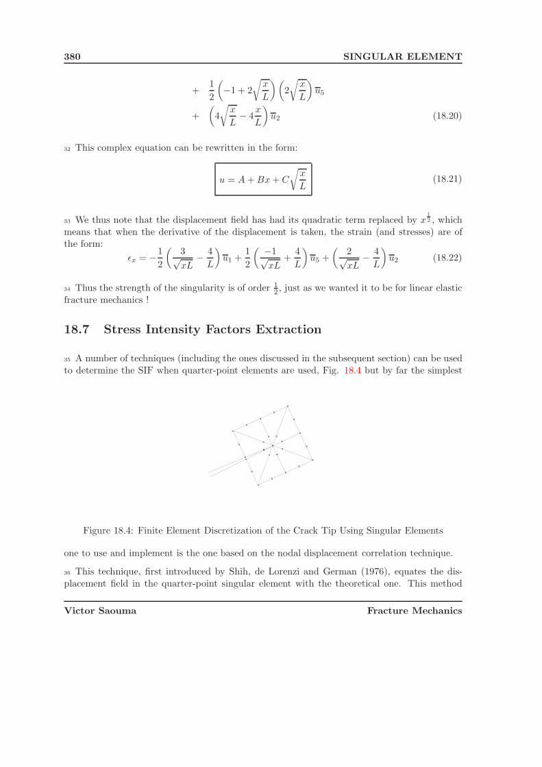
380 SINGULAR ELEMENT
+1
2
(−1 + 2
√x
L
)(2
√x
L
)u5
+
(4
√x
L− 4
x
L
)u2 (18.20)
32 This complex equation can be rewritten in the form:
u = A + Bx + C
√x
L(18.21)
33 We thus note that the displacement field has had its quadratic term replaced by x12 , which
means that when the derivative of the displacement is taken, the strain (and stresses) are ofthe form:
εx = −1
2
(3√xL
− 4
L
)u1 +
1
2
( −1√xL
+4
L
)u5 +
(2√xL
− 4
L
)u2 (18.22)
34 Thus the strength of the singularity is of order 12 , just as we wanted it to be for linear elastic
fracture mechanics !
18.7 Stress Intensity Factors Extraction
35 A number of techniques (including the ones discussed in the subsequent section) can be usedto determine the SIF when quarter-point elements are used, Fig. 18.4 but by far the simplest
Figure 18.4: Finite Element Discretization of the Crack Tip Using Singular Elements
one to use and implement is the one based on the nodal displacement correlation technique.
36 This technique, first introduced by Shih, de Lorenzi and German (1976), equates the dis-placement field in the quarter-point singular element with the theoretical one. This method
Victor Saouma Fracture Mechanics
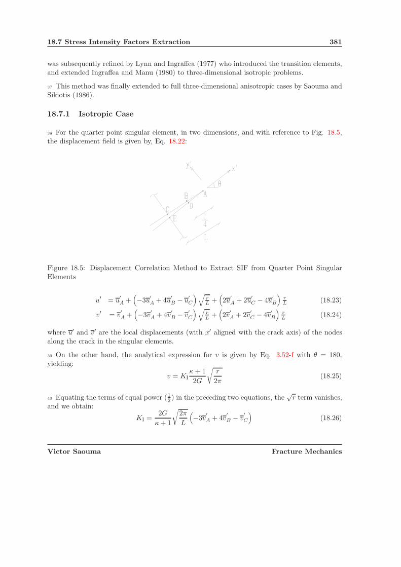
18.7 Stress Intensity Factors Extraction 381
was subsequently refined by Lynn and Ingraffea (1977) who introduced the transition elements,and extended Ingraffea and Manu (1980) to three-dimensional isotropic problems.
37 This method was finally extended to full three-dimensional anisotropic cases by Saouma andSikiotis (1986).
18.7.1 Isotropic Case
38 For the quarter-point singular element, in two dimensions, and with reference to Fig. 18.5,the displacement field is given by, Eq. 18.22:
Figure 18.5: Displacement Correlation Method to Extract SIF from Quarter Point SingularElements
u′ = u′
A +(−3u
′
A + 4u′
B − u′
C
)√rL +
(2u
′
A + 2u′
C − 4u′
B
)rL (18.23)
v′ = v′
A +(−3v
′
A + 4v′
B − v′
C
)√rL +
(2v
′
A + 2v′
C − 4v′
B
)rL (18.24)
where u′ and v′ are the local displacements (with x′ aligned with the crack axis) of the nodesalong the crack in the singular elements.
39 On the other hand, the analytical expression for v is given by Eq. 3.52-f with θ = 180,yielding:
v = KIκ + 1
2G
√r
2π(18.25)
40 Equating the terms of equal power (12 ) in the preceding two equations, the
√r term vanishes,
and we obtain:
KI =2G
κ + 1
√2π
L
(−3v
′
A + 4v′
B − v′
C
)(18.26)
Victor Saouma Fracture Mechanics

382 SINGULAR ELEMENT
41 If this approach is generalized to mixed mode problems, then the two stress intensity factorsare given by:
{KI
KII
}=
1
2
2G
κ + 1
√2π
L
[0 11 0
]⎡⎣ −3u′
A + 4(u
′
B − u′
D
)−(u
′
C − u′
E
)−3v
′
A + 4(v′
B − v′
D
)−(v′
C − v′
E
)⎤⎦ (18.27)
42 Thus it can be readily seen that the extraction of the SIF can be accomplished through a“post-processing” routine following a conventional finite element analysis in which the quarter-point elements have been used.
18.7.2 Anisotropic Case
43 Following a similar procedure to the one previously described, for the anisotropic case,1
Saouma and Sikiotis (1986) have shown that the three stress intensity factors can be evaluatedfrom: ⎧⎪⎨
⎪⎩KI
KII
KIII
⎫⎪⎬⎪⎭ = [B]−1 [A]
√2π
L(18.28)
where [A] is obtained from the displacements of those nodes along the crack in the singularquarter-point wedge element, as shown in Fig. 18.6:
[A] =
⎡⎢⎢⎢⎣
2uB − uC + 2uE − uF + uD + 12η (−4uB + uC + 4uE − uF ) + 1
2η2 (uF + uC − 2uD)
2vB − vC + 2vE − vF + vD + 12η (−4vB + vC + 4vE − vF ) + 1
2η2 (vF + vC − 2vD)
2wB − wC + 2wE − wF + wD + 12η (−4wB + wC + 4wE − wF ) + 1
2η2 (wF + wC − 2wD)
⎤⎥⎥⎥⎦ (18.29)
and [B] is obtained from the analytical solution to the displacements around the crack tip inhomogeneous anisotropic solids:
[B]−1 =
⎡⎢⎢⎢⎢⎢⎢⎢⎢⎢⎢⎢⎣
Re[
is1−s2
(q2 − q1)]
1D Re
[−i
s1−s2(p2 − p1)
]1D 0
Re[
−is1−s2
(s1q2 − s2q1)]
1D Re
[i
s1−s2(s1p2 − s2p1)
]1D 0
0 0 1
(c44c55−c245)
⎤⎥⎥⎥⎥⎥⎥⎥⎥⎥⎥⎥⎦
(18.30)
1Anisotropic modelling is important for either roller compacted concrete dams or layered rock foundations.
Victor Saouma Fracture Mechanics

18.8 Numerical Evaluation 383
Figure 18.6: Nodal Definition for FE 3D SIF Determination
18.8 Numerical Evaluation
44 Based on an extensive parametric study, Saouma and Schwemmer (1984), have formulatedthe following recommendations for the use of the singular quarter point element:
1. Use a 2 × 2 (reduced) integration scheme.
2. Use at least four (in pure mode I problems), or eight (in mixed mode problems) singularelements around a crack tip.
3. Have the internal angles of all the singular elements around the crack tip approximatelyequal to 45 degrees.
4. Unless an excessively small l/a ratio is used, little improvement is achieved by usingtransition elements.
5. For problems with uniform non-singular stress distribution, little improvement is achievedby using a small l/a.
6. For problems where a non-singular, stress gradient is expected, l/a should be less than0.5.
Victor Saouma Fracture Mechanics

384 SINGULAR ELEMENT
45 Note that the above recommendations remain valid in mixed mode crack propagation studies.Although initially they cannot be directly extended to cases with high KII
KI, it is well known
that the crack tends to propagate in a direction that minimizes (but not completely eliminates)KII where the above recommendations would be valid.
18.9 Historical Overview
46 Because quarter point have been so popular (and still are) in light of their simplicity, thissection will provide an overview of the major extensions to this simple method to determineSIF.
47 Barsoum (1974) and Henshell and Shaw (1975) independently demonstrated that the inversesquare root singularity characteristic of linear elastic fracture mechanics can be obtained inthe 2D 8-noded isoparametric element (Q8) when the mid-side nodes near the crack tip areplaced at the quarter point. This concept was subsequently extended to plate bending andshell fractures by Barsoum (1975) andBarsoum (1976a).
48 Barsoum (1976b) then showed that the triangular element formed by collapsing one side ofthe Q8 led to far better results than the rectangular element. Freese and Tracy (1976) showedthat the natural isoparametric triangle (NIT) and the collapsed quadrilateral perform equallywell. If the side opposite to the crack tip is curved, than there is a substantial deterioration in theSIF calculation from the collapsed quadrilateral, and no change in the NIT. Such a discrepancyis caused by the fact that a collapsed 8-node quadrilateral does not actually degenerate into anNIT (Newton 1973).
49 The extension of the quadratic isoparametric quarter-point element to cubic isoparametricwas proposed by Pu, Hussain and Lorensen (1977). Yamada, Ezawa and Nishiguchi (1979)extended the concept of the 8-node isoparametric element to the variable numbering element.
50 Hibbitt (1977) proved that the singular rectangular element has a singular stiffness whereasthe triangular one does not, and that in the collapsed quadrilateral element the singularityprevails along the two sides only, whereas it is omnipresent inside the triangular element. Heattributed this difference to the better results achieved by the triangular element as reportedby Barsoum. He also demonstrated that a variety of stress singularities (1/n) can be achievedby isoparametric elements with a polynomial approximation of order n. In a recent paper,Ying (1982) showed that in his investigation Hibbitt erroneously concluded that the strainenergy of a rectangular quarter-point element is singular, but that, as previously known, thesingularity is along the edges and diagonal only. Also discussed by Ying is the error associatedwith the location of the quarter-point of a singular element. This was further elaborated onby Barsoum’s discussion of the previous work (Barsoum 1982), in which he has shown that theerror in estimating the SIF is one order of magnitude smaller than the discretization error inlocating the quarter-point. Hence the exact location of the mid-side node is not crucial as longas the discretization error is small. Also by having multiple independent nodes (of a collapsed
Victor Saouma Fracture Mechanics
18.9 Historical Overview 385
Q8), Barsoum (1977) showed that small-scale yielding (characterized by 1/r stress singularity)could be modelled.
51 Lynn and Ingraffea (1977) generalized the concept of the quarter-point singular elementand showed that by varying the placement of the side node, between quarter- and mid-point,one can control the point where singularity is to occur (between the corner node and infinity,respectively). This led to the introduction of the transition element, which, when insertedaround the singular elements, resulted in improved SIF calculations as the l/a (element lengthover total crack length) ratio decreased. Again Hussain, Vasilakis and Pu (1981) extended theconcept of quadratic transition elements to cubic transition elements.
52 In his dissertation, Ingraffea (1977) investigated both the effect of the l/a and aspect ratioof the singular elements. An optimum ratio of l/a=0.25 was reported, and it was found thatthe aspect ratio effect was relatively unimportant. This dependency of the SIF on the l/a ratiowas subsequently further described by Lynn and Ingraffea. Another detailed investigation ofthe optimum quarter point-element size was carried out by Ingraffea and Manu (1980), wherel/a was varied from 0.2 to 0.03 in both two- and three-dimensional analyses. The errors in thetwo-dimensional results varied from -8 percent for l/a = 0.20 to -1 percent for l/a = 0.03.
53 An assessment of the quarter-point elements (in pressure vessel fracture analysis) was offeredby Barsoum (1981) for both two- and three-dimensional analysis. Three sources of modellingerrors associated with the quarter-point elements were discussed: (a) those associated withthe type of quarter-point element, triangular or rectangular; (b) those associated with theconfiguration of the element boundary, straight or curved; and (c) those associated with thelocation of the quarter-point node. Barsoum indicated that (a) triangular elements are to bepreferred over the quadrilateral ones (whether collapsed or not); (b) the sides of the elementshould not be curved; and (c) perturbation of the quarter-point node by e leads to an errorin calculating the stress intensity factor of ge2 where g is the ratio of the crack tip element tocrack length.
54 In a recent paper, Harrop (1982) qualitatively discussed the optimum size of quarter-pointcrack tip elements. He indicated that the singular element can represent the stress singularityand a constant finite stress term only. Thus any singular element that is too large cannotrepresent a structure non-linear (and non-singular) stress variation. On the other hand, byusing a singular element that is too small, the error in representing the finite stress termdecreases, but the region of the mesh representing the stress singularity also decreases. Thissource of error would still hold even if transition elements were used. He thus pointed out thatsome crack tip element size has to be optimum, and concluded that “it is clearly impossible torecommend a particular crack tip element size suitable for all situations.”
55 An assessment of various crack tip singular elements for use with isoparametric elements wasdiscussed by Fawkes, Owen and Luxmoore (1979). In this study, elements based on the use ofdistorted shape functions, standard shape functions, analytical solutions, superposition process,and hybrid techniques were evaluated using a test problem of both single and combined modefracture. This study revealed that the best results were achieved by the analytic element, and
Victor Saouma Fracture Mechanics

386 SINGULAR ELEMENT
the next best group was the one using the distorted shape function.
56 Few of the above papers discussed the numerical accuracy achieved by the quarter-pointelement in any detail or attempted to provide recommendations for its best usage. At bestthere have been conflicting indications, usually based on few analyses, on the appropriate l/aratio to be used. Also one of the major arguments expressed against the use of this element isthe SIF dependency on l/a. Furthermore, in light of a new generation of computer programs(Saouma and Zatz 1984), which simulates the discrete crack propagation inside a finite elementmesh with automatic remeshing, it is important to quantify the discretization error associatedwith the quarter-point singular element.
57 It is clear that such a numerical evaluation of this increasingly popular element is longoverdue. It should provide the stress analyst (who could be using a general purpose finiteelement program) with guidelines for the mesh preparation around the crack tip and some ideaabout the level of accuracy to be expected from the analysis.
58 In the present study, two problems with known analytical stress intensity factors are consid-ered. A number of parameters will be varied during the executions, and numerical values of thestress intensity factors will be compared to the exact ones. From the numerous analyses, a database will be created and graphically represented. It is anticipated that, through appropriateand careful interpretation of those results, guidelines for the mesh preparation around the cracktip could be achieved along with an approximate evaluation of the resulting accuracy.
18.10 Other Singular Elements
59 For the most part this section discussed only the quarter point element, but one should beaware of the following alternative formulations:
1. exact field modelling (Rao, Raju and Krishna Murty 1971), (Apostal 1974)
2. hybrid elements by Atluri, Kobayachi and Nakagaki (1979)
3. enriched elements by Benzley (1974), in which the shape functions are enriched withadditional terms, which account for the singular terms:
ui =4∑
k=1
fkuik + KI
(Q1i
4∑k=1
fkQ1ik
)+ KII
(Q2i
4∑k=1
fkQ2ik
)(18.31)
Qij =uij
ki(18.32)
u′ =
(1 +
2x
L− 3
√x
L
)u
′
1 +
(4
√x
L− 4
x
L
)u
′
2 +
(2x
L−√
x
L
)u
′
3 (18.33)
60 In this method the stress intensity factors are treated as primary unknowns, and arethus obtained during the global stiffness matrix decomposition. Although this method
Victor Saouma Fracture Mechanics

18.10 Other Singular Elements 387
has yielded some very good results, its main drawback is that the finite element programhas to be altered in order to implement it. This method was first proposed by Benzleywhen the quarter-point element (discussed in the next chapter) was not yet known.
Victor Saouma Fracture Mechanics

388 SINGULAR ELEMENT
Victor Saouma Fracture Mechanics

Chapter 19
ENERGY RELEASE BASEDMETHODS
1 In this class of solutions, we will exploit the definition of the energy release rate G to derive asimple method of determining the stress intensity factors. We shall distinguish between modeI and mixed mode cases. The former one, although of academic relevance only, is a simpleintroduction to the second.
19.1 Mode I Only
19.1.1 Energy Release Rate
2 Recalling that the strain energy release rate G is given by:
G = −∂U
∂a=
K2I
E′ � ΔU
Δa(19.1)
a simple algorithm for the SIF calculation emerges:
1. For an initial crack length a, determine the total strain energy from either one of thefollowing approaches:
(a) U = utKu where u is nodal displacement, and K is the global structural stiffnessmatrix.
(b) U = utP where P and u are the externally applied nodal load and displacement,respectively.
2. Increase the crack length from a to a + Δa, Fig. 19.1, and reanalyze.
3. Determine G from G � (U+ΔU)−U(a+Δa)−a = ΔU
Δa =K2
I
E′

390 ENERGY RELEASE BASED METHODS
aΔ
Figure 19.1: Crack Extension Δa
3 Note that:
1. This procedure requires two complete separate analyses.
2. The stress singularity need not be modelled.1
3. This technique is restricted to mode I only.
4. Usage of an over-relaxation solver (such as the Gauss-Seidel) can reduce computationaltime for the second analysis in which the global stiffness matrix is only slightly altered.
19.1.2 Virtual Crack Extension.
4 As previously noted, the stiffness matrix is only slightly perturbed in the second analysis(associated with a+Δa); thus both Parks (1974) and Hellen (1975) have independently proposeda modification of the preceding approach2.
5 The potential energy Π is given by:
Π =1
2�u[K]{u} − �u{p} (19.2)
1It has nevertheless been shown that slightly improved results can be obtained if quarter-point elements areused.
2This same technique is now given two different names: stiffness derivative (Park) and virtual crack extension(Hellen).
Victor Saouma Fracture Mechanics

19.2 Mixed Mode Cases 391
and
− G =∂Π
∂a= ∂�u
∂a [K]{u} + 12�u
∂[K]∂a {u} − ∂�u
∂a {P} − �u∂{P}∂a
= −∂�u∂a ([K]{u} − {P})︸ ︷︷ ︸
0
+12�u
∂[K]∂a {u} − �u∂{P}
∂a (19.3)
6 Noting that the first term in the last equation is zero, we obtain:
G = −1
2�u∂[K]
∂a{u} + �u∂{P}
∂a(19.4)
7 Thus if the load is unaltered during the crack extension, than the energy release rate is directlyrelated to the derivative of the stiffness.
8 Finally, we note that:
1. Only the portion of the stiffness matrix associated with the elements surrounding thecrack tip needs to be perturbed.
2. Better results are obtained if singular elements are used.
3. The method can easily be generalized to three-dimensional problems.
4. It can be shown (Parks 1974) that this technique is equivalent to the determination ofthe J integral.
5. This method is restricted to mode I loading only.
19.2 Mixed Mode Cases
9 Having presented two simple techniques for the SIF extraction for pure mode I cases, we nowgeneralize them to mixed mode loading.
19.2.1 Two Virtual Crack Extensions.
10 A major limitation of the preceding methods is that in its present form it does not distinguishthe mode I from the mode II components in the energy release rate. Such a “discrimination”is possible if we take into account the expressions of the energy release rate obtained by Hellenand Blackburn (1975b) in which:
J1 = G1 =K2
I + K2II
E′ +K2
III
2μ(19.5)
J2 = G2 =−2KIKII
E′ (19.6)
Victor Saouma Fracture Mechanics
392 ENERGY RELEASE BASED METHODS
where E′ = E for plane stress, and E′ = E1−ν2 for plane strain. G1 and G2 are associated with
virtual crack extensions at θ = 0 and θ = π2 respectively.
11 Based on this decomposition of G, the algorithm for SIF extractions in mixed mode problemsusing virtual crack extensions is as follows:
1. For an initial crack length a, determine the total strain energy U .
2. Extend the crack length from a to a + Δa:
(a) Along θ = 0, and determine G1.
(b) Along θ = π2 , and determine G2.
3. Solve for the two SIF from:
KI =s ±
√s2 + 8G2
α
2
KII =s ∓
√s2 + 8G2
α
2
(19.7)
where s = 2√
G1−G2α and α = (1+ν)(1+κ)
E
12 An alternative to this technique is to use G(θ) = G1 cos(θ) + G2 sin(θ), and use two distinctvalues of θ, which are not necessarily 0 or π
2 .
19.2.2 Single Virtual Crack Extension, Displacement Decomposition
13 A major disadvantage of the preceding techniques is that at least one complete finite elementanalysis is required, followed by either two separate ones or two virtual crack extensions. Inthe single solution displacement decomposition method of Sha (1984) and Ishikawa (1980), wehave a technique in which only one analysis is required.
14 With reference to Fig. 19.2, we can decompose the nodal displacements into two localcomponents:
Δ = Δ1 + Δ2 (19.8)
where
{Δ1} =
{u1
v1
}=
1
2
{u + u′
v − v′
}
{Δ2} =
{u2
v2
}= 1
2
{u − u′
v + v′
} (19.9)
Victor Saouma Fracture Mechanics
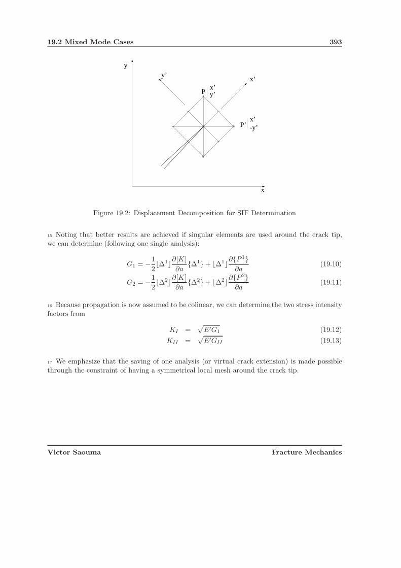
19.2 Mixed Mode Cases 393
x
y
P
P’
x’y’
x’y’
x’-y’
Figure 19.2: Displacement Decomposition for SIF Determination
15 Noting that better results are achieved if singular elements are used around the crack tip,we can determine (following one single analysis):
G1 = −1
2�Δ1∂[K]
∂a{Δ1} + �Δ1∂{P 1}
∂a(19.10)
G2 = −1
2�Δ2∂[K]
∂a{Δ2} + �Δ2∂{P 2}
∂a(19.11)
16 Because propagation is now assumed to be colinear, we can determine the two stress intensityfactors from
KI =√
E′G1 (19.12)
KII =√
E′GII (19.13)
17 We emphasize that the saving of one analysis (or virtual crack extension) is made possiblethrough the constraint of having a symmetrical local mesh around the crack tip.
Victor Saouma Fracture Mechanics

394 ENERGY RELEASE BASED METHODS
Victor Saouma Fracture Mechanics

Chapter 20
J INTEGRAL BASED METHODS
20.1 Numerical Evaluation
1 Within linear elastic fracture mechanics, the J integral is equivalent to G and we have:
G = J = −∂Π
∂a=
∫r(wdy − t · ∂d
∂xds) (20.1)
2 Thus it is evident that we do have two methods of evaluating J : the first one stems from itsequivalence to the energy released rate, and the second one from its definition as an integralalong a closed contour. Evaluation of J according to the first approach is identical to the oneof G and has been previously presented.
3 In this chapter we shall present the algorithm to evaluate J on the basis of its contour lineintegral definition. Whereas derivation will be for J integral only, its extension to Ji is quitestraightforward.
4 If the stresses were to be determined at the nodes, than the numerical evaluation of J willbe relatively simple. However, most standard finite element codes only provide Gauss pointstresses, and hence care must be exercised in properly determining the J integral along a pathpassing through them.
5 The algorithm for the J calculation closely follows the method presented in (Owen and Fawkes1983), and is as follows:
1. First let us restrict ourselves to the more general case in which isoparametric elementsare used. Because the stresses are most accurately evaluated at the gauss points, thepath can be conveniently chosen to coincide with ξ = ξcst and/or η = ηcst. For the sakeof discussion, let us assume that the element connectivity is such that the path is alongξ = ξcst, as in Fig. 20.1. We note that for corner elements the integration will have to beperformed twice along the two directions.

396 J INTEGRAL BASED METHODS
ξ=ξ
x
y
nGauss PointNumberingSequence
cst
xx x
xxx x
14 7
536 9
x
x2
8
ηξ
Figure 20.1: Numerical Extraction of the J Integral (Owen and Fawkes 1983)
2. Now let us start from the basic definition of J :
J =
∫Γ
wdy − t · ∂d
∂xds (20.2)
where t is the traction vector along n, which is normal to the path; d is the displacementvector; ds is the element of arc along path Γ; and w is the strain energy density. We notethat the crack is assumed to be along the x axis. If it is not, stresses and displacementswould first have to be rotated. Let us now determine each term of Eq. 20.2.
3. The traction vector is given by:
ti = σijnj ⇒ t =
{σxxn1 + τxyn2
τxyn1 + σyyn2
}(20.3)
4. The displacement vector is:
d =
{uv
}(20.4)
5. The strain energy density w is:
w =1
2(σxxεxx + 2τxyγxy + σyyεyy)
=1
2[σxx
∂u
∂x+ τxy(
∂u
∂y+
∂v
∂x) + σyy
∂v
∂y] (20.5)
Victor Saouma Fracture Mechanics

20.1 Numerical Evaluation 397
6. The arc length ds and dy are given by:
ds =√
dx2 + dy2 =
√(∂x
∂η
)2
+
(∂y
∂η
)2
dη (20.6)
=∂y
∂ηdη (20.7)
7. Next we can evaluate part of the second term of J :
t · ∂d
∂x= (σxn1 + τxyn2)
∂u
∂x+ (τxyn1 + σyn2)
∂v
∂x(20.8)
where n1 and n2 are the components of n, which is a unit vector normal to the contourline at the Gauss point under consideration.
8. Having defined all the terms of J , we substitute in Eq. 20.2 to obtain the contribution toJ from a particular Gauss point within an element.
Je =
∫ 1
−1
⎧⎪⎪⎪⎪⎨⎪⎪⎪⎪⎩
1
2
[σx
∂u
∂x+ τxy
(∂u
∂y+
∂v
∂x
)+ σy
∂v
∂y
]︸ ︷︷ ︸
w
∂y
∂η︸︷︷︸dy
−[(σxn1 + τxyn2)
∂u
∂x+ (τxyn1 + σyn2)
∂v
∂x
]︸ ︷︷ ︸
t· ∂d
∂x
√(∂x
∂η
)2
+
(∂y
∂η
)2
︸ ︷︷ ︸ds
⎫⎪⎪⎪⎪⎬⎪⎪⎪⎪⎭
dη (20.9)
=
∫ 1
−1Idη
9. Since the integration is to be carried out numerically along the path (using the sameintegration points used for the element stiffness matrix), we have:
Je =NGAUS∑
q=1
I(ξp, ηq)Wq (20.10)
where Wq is the weighting factor corresponding to ηq and NGAUS is the order of inte-gration (2 or 3).
10. Stresses σx, σy, τxy are readily available at the Gauss points.
Victor Saouma Fracture Mechanics

398 J INTEGRAL BASED METHODS
11. ∂u∂x , ∂u
∂y , ∂v∂x , and ∂v
∂y are obtained through the shape function. For instance ∂u∂x = �∂Ni
∂x {ui}where the ui are the nodal displacements and ∂Ni
∂x is the cartesian derivative of the shapefunction stored in the [B] matrix:
[B] =
⎡⎢⎣
∂Ni
∂x 0
0 ∂Ni
∂y∂Ni
∂y∂Ni
∂x
⎤⎥⎦ (20.11)
where i ranges from 1 to 8 for quadrilateral elements.
12. Another term not yet defined in Eq. 20.9 is ∂y∂η . This term is actually stored already in
the Gauss point Jacobian matrix:
[J ] =
[∂x∂ξ
∂y∂ξ
∂x∂η
∂y∂η
](20.12)
13. Finally we are left to determine n1 and n2 (components of n). Since there is an infinitenumber of vectors normal to ξ, and we want the one which is in the ξη plane, the normalis determined as follows:
(a) Define two arbitrary vectors: A along ξ = ξcst and B along η = ηcst such that:
At = � ∂x∂η , ∂y
∂η , 0 (20.13)
Bt = � ∂x∂ξ , ∂y
∂ξ , 0 (20.14)
Note that we have defined the three-dimensional components of those two vectors.
(b) Now we define a third vector, which is normal to the plane defined by the precedingtwo: C = A× B, or: ⎡
⎢⎣i j k
∂x∂η
∂y∂η 0
∂x∂ξ
∂y∂ξ 0
⎤⎥⎦ (20.15)
This leads to:
C = � 0, 0, ∂x∂η
∂y∂ξ − ∂y
∂η∂x∂ξ (20.16)
(c) With C defined, we can now return to the original plane and define
D = C ×A ⇒ D = �∂y
∂η(∂y
∂η
∂x
∂ξ− ∂x
∂η
∂y
∂ξ)︸ ︷︷ ︸
D1
,∂x
∂η(∂x
∂η
∂y
∂ξ− ∂y
∂η
∂x
∂ξ)︸ ︷︷ ︸
D2
, 0 (20.17)
Victor Saouma Fracture Mechanics
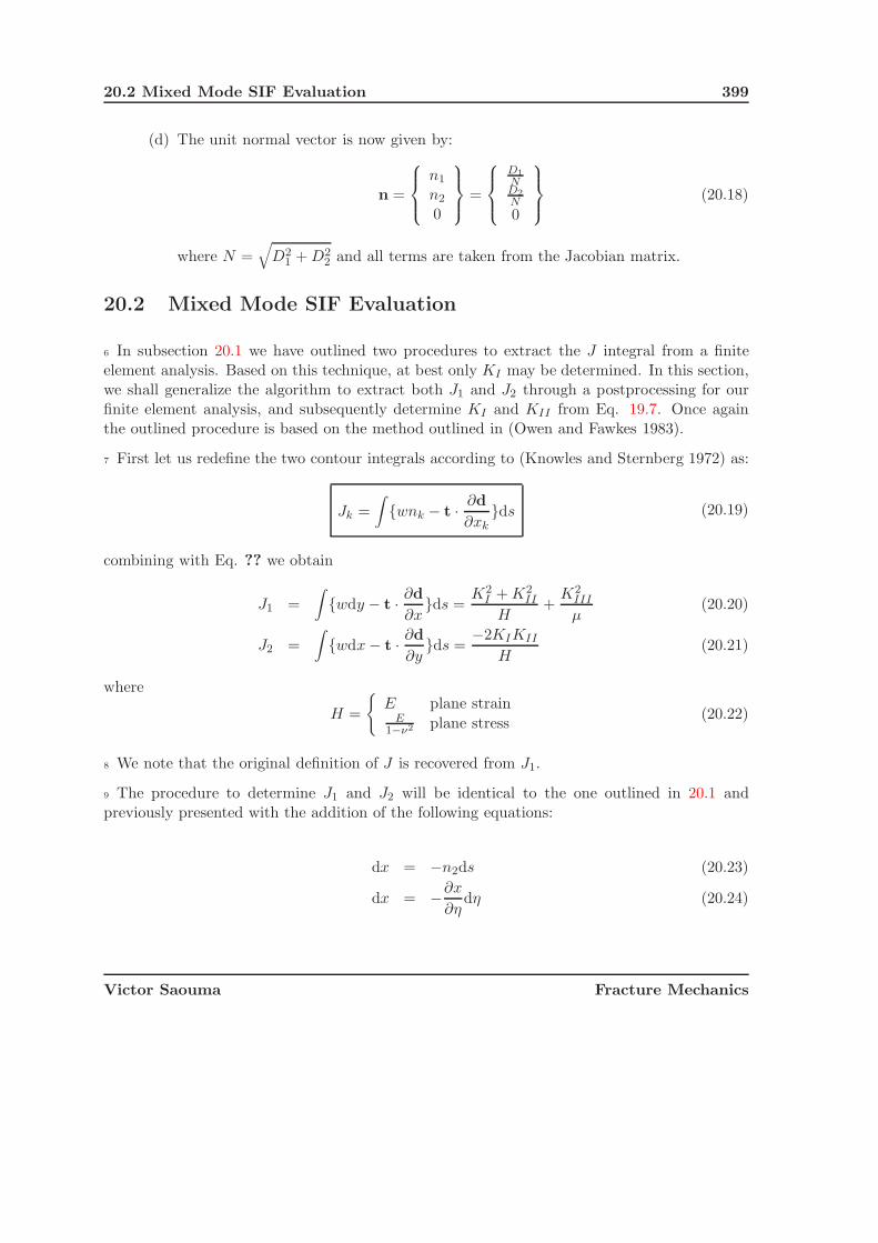
20.2 Mixed Mode SIF Evaluation 399
(d) The unit normal vector is now given by:
n =
⎧⎪⎨⎪⎩
n1
n2
0
⎫⎪⎬⎪⎭ =
⎧⎪⎨⎪⎩
D1ND2N0
⎫⎪⎬⎪⎭ (20.18)
where N =√
D21 + D2
2 and all terms are taken from the Jacobian matrix.
20.2 Mixed Mode SIF Evaluation
6 In subsection 20.1 we have outlined two procedures to extract the J integral from a finiteelement analysis. Based on this technique, at best only KI may be determined. In this section,we shall generalize the algorithm to extract both J1 and J2 through a postprocessing for ourfinite element analysis, and subsequently determine KI and KII from Eq. 19.7. Once againthe outlined procedure is based on the method outlined in (Owen and Fawkes 1983).
7 First let us redefine the two contour integrals according to (Knowles and Sternberg 1972) as:
Jk =
∫{wnk − t · ∂d
∂xk}ds (20.19)
combining with Eq. ?? we obtain
J1 =
∫{wdy − t · ∂d
∂x}ds =
K2I + K2
II
H+
K2III
μ(20.20)
J2 =
∫{wdx − t · ∂d
∂y}ds =
−2KIKII
H(20.21)
where
H =
{E plane strain
E1−ν2 plane stress
(20.22)
8 We note that the original definition of J is recovered from J1.
9 The procedure to determine J1 and J2 will be identical to the one outlined in 20.1 andpreviously presented with the addition of the following equations:
dx = −n2ds (20.23)
dx = −∂x
∂ηdη (20.24)
Victor Saouma Fracture Mechanics

400 J INTEGRAL BASED METHODS
20.3 Equivalent Domain Integral (EDI) Method
10 In this section, we shall derive an alternative expression for the energy release rate. Contrarilyto the virtual crack extension method where two analyses (or a stiffness derivative) had to beevaluated, in this method, we have to perform only one analysis. The method is really based onRice’s J integral. However, it is recognized that evaluation of J in 2D involves a line integralonly and a line integral plus a volume integral if body forces are present, (deLorenzi, H.G. 1985).For 3D problems, the line integral is replaced by a surface integral (and a volume integral forbody forces).
11 Recognizing that surface integrals may not be easily evaluated in 3D, Green’s theorem isinvoked, and J will be evaluated through a volume integral in 3D and a surface integral in 2D.Thus computationally, this method is quite attractive.
12 Again as for the previous case, we will start by evaluating the energy release rate, and onlysubsequently we shall derive expressions for the SIF.
13 The essence of the method consists in replacing the contour integral, by a closed integral(outer and inner) while multiplying the expression of J by a function q equal to zero on the outersurface and unity on the inner one. We adopt the expression of J derived for a propagatingcrack (thus determined around a path close to the crack tip). Having defined a closed path, wethen apply Green’s theorem, and replace a contour integral by a surface integral.
20.3.1 Energy Release Rate J
20.3.1.1 2D case
14 Recalling the expression for the energy release rate of a propagating crack, Eq. 11.126
J = limΓ0→0
∫Γ0
[(w + T ) δ1i − σij
∂uj
∂x1
]nidΓ (20.25)
where w is the strain energy density, T is the kinetic energy
T =1
2ρ∂ui
∂t
∂ui
∂t(20.26)
and δ the Kronecker delta.
15 An alternative form of this equation (Anderson 1995) is
J = limΓ0→0
∫Γ0
[(w + T ) dy − σijni
∂uj
∂xdΓ
](20.27)
Unlike the conventional J integral, the contour path for this equation can not be arbitrarilyselected.
Victor Saouma Fracture Mechanics
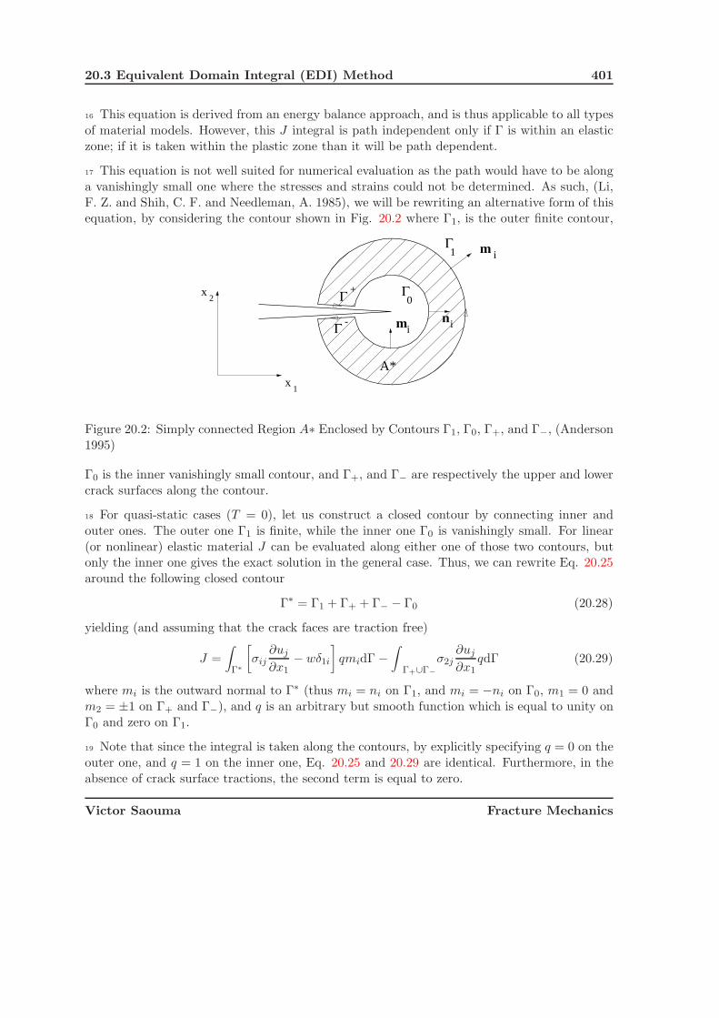
20.3 Equivalent Domain Integral (EDI) Method 401
16 This equation is derived from an energy balance approach, and is thus applicable to all typesof material models. However, this J integral is path independent only if Γ is within an elasticzone; if it is taken within the plastic zone than it will be path dependent.
17 This equation is not well suited for numerical evaluation as the path would have to be alonga vanishingly small one where the stresses and strains could not be determined. As such, (Li,F. Z. and Shih, C. F. and Needleman, A. 1985), we will be rewriting an alternative form of thisequation, by considering the contour shown in Fig. 20.2 where Γ1, is the outer finite contour,
0Γ
x
x
1
2
Γ1
Γ
Γ -
+
A*
m
m
i
i
ni
Figure 20.2: Simply connected Region A∗ Enclosed by Contours Γ1, Γ0, Γ+, and Γ−, (Anderson1995)
Γ0 is the inner vanishingly small contour, and Γ+, and Γ− are respectively the upper and lowercrack surfaces along the contour.
18 For quasi-static cases (T = 0), let us construct a closed contour by connecting inner andouter ones. The outer one Γ1 is finite, while the inner one Γ0 is vanishingly small. For linear(or nonlinear) elastic material J can be evaluated along either one of those two contours, butonly the inner one gives the exact solution in the general case. Thus, we can rewrite Eq. 20.25around the following closed contour
Γ∗ = Γ1 + Γ+ + Γ− − Γ0 (20.28)
yielding (and assuming that the crack faces are traction free)
J =
∫Γ∗
[σij
∂uj
∂x1− wδ1i
]qmidΓ −
∫Γ+∪Γ−
σ2j∂uj
∂x1qdΓ (20.29)
where mi is the outward normal to Γ∗ (thus mi = ni on Γ1, and mi = −ni on Γ0, m1 = 0 andm2 = ±1 on Γ+ and Γ−), and q is an arbitrary but smooth function which is equal to unity onΓ0 and zero on Γ1.
19 Note that since the integral is taken along the contours, by explicitly specifying q = 0 on theouter one, and q = 1 on the inner one, Eq. 20.25 and 20.29 are identical. Furthermore, in theabsence of crack surface tractions, the second term is equal to zero.
Victor Saouma Fracture Mechanics

402 J INTEGRAL BASED METHODS
20 Applying the divergence theorem to Eq. 20.29∮Γv.n =
∫A
(∂vx
∂x+
∂vy
∂y
)dxdy (20.30)
we obtain
J =
∫A∗
∂
∂xi
{[σij
∂uj
∂x1− wδ1i
]q
}dA (20.31)
=
∫A∗
[(σij
∂uj
∂x1− wδ1i
)∂q
∂xi+
(∂
∂xi
(σij
∂uj
∂x1
)− ∂w
∂x1
)q
]dA (20.32)
where A∗ is the area enclosed by Γ∗.
21 Let us show that the second term is equal to zero:
∂
∂xi
(σij
∂uj
∂x1
)= σij
∂
∂xi
(∂uj
∂x1
)︸ ︷︷ ︸
∂w∂x
+∂σij
∂xi︸ ︷︷ ︸0
∂ui
∂x1(20.33)
however from equilibrium we have∂σij
∂xi= 0 (20.34)
22 Furthermore, the derivative of the strain energy density is
∂w
∂x=
∂w
∂εij
∂εij
∂x= σij
∂εij
∂x(20.35)
substituting
εij =1
2
(∂ui
∂xj+
∂uj
∂xi
)(20.36)
we obtain∂w
∂x=
1
2σij
[∂
∂x
(∂ui
∂xj
)+
∂
∂x
(∂uj
∂xi
)]= σij
∂
∂xj
(∂ui
∂x
)(20.37)
23 Hence, it is evident that the second term of Eq. 20.32 vanishes and that we are left with
J =
∫A∗
[σij
∂ui
∂x1− wδ1i
]∂q
∂xidA (20.38)
This expression, is analogous to the one proposed by Babuska for a surface integral basedmethod to evaluate stress intensity factors, (Babuska and Miller 1984).
24 We note that deLorenzi (deLorenzi, H.G. 1985) has shown that the energy release rate isgiven by
G =1
ΔA
∫ (σij
∂uj
∂x1− wδi1
)∂Δx1
∂xidA (20.39)
Victor Saouma Fracture Mechanics

20.3 Equivalent Domain Integral (EDI) Method 403
for a unit crack growth extension along x1. Thus comparing Eq. 20.38 with 20.39, we observethat the two expressions are identical for q = Δx1
Δa , and thus q can be interpreted as a normalizedvirtual displacement. In this context it was merely a mathematical device.
25 In summary, we have replace a contour integral by an equivalent area integral to determineJ .
20.3.1.2 3D Generalization
26 In this section, we shall generalize to 3D our previous derivation, (Anderson 1995). FromFig. 20.3 we define a local coordinate system such that x1 is normal to the crack front, x2
normal to the crack plane, and x3 tangent to the crack front.
Figure 20.3: Surface Enclosing a Tube along a Three Dimensional Crack Front, (Anderson 1995)
27 For an arbitrary point, the J integral is given by Eq. 20.25. We now consider a tube oflength ΔL and radius r0 that surrounds the segment of the crack front under consideration.We now define a weighted average J over the crack front segment of length ΔL as
JΔL =
∫ΔL
J(η)qdη (20.40)
= limr0→0
∫S0
[wδ1i − σij
∂uj
∂x1
]qnids (20.41)
where J(η) is the point-wise value of J , S0 is the vanishingly small surface area of the tube,q is the weight function previously introduced. q can be again interpreted as a virtual crackadvance and Fig. 20.4 illustrates an incremental crack advance over ΔL where q is defined as
Victor Saouma Fracture Mechanics

404 J INTEGRAL BASED METHODS
aΔ max aΔ maxq
LΔ
Figure 20.4: Interpretation of q in terms of a Virtual Crack Advance along ΔL, (Anderson 1995)
Δa(η) = q(η)Δamax (20.42)
and the corresponding incremental area of the virtual crack is
ΔAc = Δamax
∫ΔL
q(η)dη (20.43)
28 As in the previous case, this expression of J can not be numerically determined for a vanish-ingly small radius r0, as such and as in the previous 2D case, we define a second tube of radiusr1 around the crack front, Fig. 20.5.
Figure 20.5: Inner and Outer Surfaces Enclosing a Tube along a Three Dimensional CrackFront
Victor Saouma Fracture Mechanics
20.3 Equivalent Domain Integral (EDI) Method 405
JΔL =
∮S∗
[σij
∂ui
∂x1− wδ1i
]qmidS −
∮S−∪S+
σ2j∂uj
∂x1qds (20.44)
whereS∗ = S1 + S+ + S− − S0 (20.45)
and S+ and S− are the upper and lower crack surfaces respectively, S0 and S1 the inner andouter tube surfaces. Note that this equation is the 3D counterpart of Eq. 20.29 which waswritten in 2D.
29 Applying the divergence theorem, this equation reduces to a volume integral
JΔL =
∫V ∗
{[σij
∂uj
∂x1− wδ1i
]∂q
∂xi+
[− ∂w
∂x1+
∂
∂xj
(σij
∂ui
∂x1
)]q
}dV
+
∫A1∪A2
(wδ1i − σij
∂ui
∂x1δ1i
)qdA
(20.46)
and q must be equal to zero at either end of ΔL that is on A1 and A2. In (Nikishkov, G.P. and Atluri, S. N. 1987) it is shown that in the absence of non-elastic (thermal and plastic)deformations the second term would be equal to zero. The third term will also be equal to zerobecause q is arbitrarily selected to be zero at each end.
20.3.2 Extraction of SIF
30 From Eq. 20.46 it is impossible to extract the 3 distinct stress intensity factors. Hence weshall generalize this equation and write it as (Nikishkov, G. P. and Atluri, S. N. 1987) (ignoringthe second and third terms)
JkΔL =
∫V ∗
(σij
∂ui
∂xk
∂q
∂xj− w
∂q
∂xk
)dV (20.47)
31 Note that k = 1, 2 only thus defining G1 = J1 and G2 = J2. However, (Nikishkov, G. P. andAtluri, S. N. 1987) have shown that G3 has a similar form and is equal to
GIII =
∫V ∗
(σ3j
∂u3
∂x1
∂q
∂xj− wIII ∂q
∂x1
)dV (20.48)
32 With G1, G2 and G3 known we need to extract the three stress intensity factors KI , KII
and KIII . Again there are two approaches.
Victor Saouma Fracture Mechanics

406 J INTEGRAL BASED METHODS
20.3.2.1 J Components
33 Based on the solution by Nikishkov, (Nikishkov and Vainshtok 1980)
KI = 12
√E∗(√
(J1 − J2 − G3) +√
(J1 + J2 − G3))
KII = 12
√E∗(√
(J1 − J2 − G3) −√
(J1 + J2 − G3))
KIII =√
2μG3
(20.49)
where, (Nikishkov, G. P. and Atluri, S. N. 1987)
E∗ = E
[1
1 − ν2+
(ν
1 + ν
)ε33
ε11 + ε22
](20.50)
which is a weighted value of E such that we retrieve E∗ = E1−ν2 for plane strain and E∗ = E
for plane stress.
20.3.2.2 σ and u Decomposition
34 As for the solution by Shah, we can decompose the displacement field as
{u} ={uI}
+{uII}
+{uIII
}
= 12
⎧⎪⎨⎪⎩
u1 + u′1
u2 − u′2
u3 + u′3
⎫⎪⎬⎪⎭+ 1
2
⎧⎪⎨⎪⎩
u1 − u′1
u2 + u′2
0
⎫⎪⎬⎪⎭+ 1
2
⎧⎪⎨⎪⎩
00
u3 − u′3
⎫⎪⎬⎪⎭
(20.51)
similarly the stresses are decomposed as
{σ} ={σI}
+{σII}
+{σIII
}
= 12
⎧⎪⎪⎪⎪⎪⎪⎪⎨⎪⎪⎪⎪⎪⎪⎪⎩
σ11 + σ′11
σ22 + σ′22
σ33 + σ′33
σ12 − σ′12
σ23 − σ′23
σ31 − σ′31
⎫⎪⎪⎪⎪⎪⎪⎪⎬⎪⎪⎪⎪⎪⎪⎪⎭
+ 12
⎧⎪⎪⎪⎪⎪⎪⎪⎨⎪⎪⎪⎪⎪⎪⎪⎩
σ11 − σ′11
σ22 − σ′22
0σ12 + σ′
12
00
⎫⎪⎪⎪⎪⎪⎪⎪⎬⎪⎪⎪⎪⎪⎪⎪⎭
+ 12
⎧⎪⎪⎪⎪⎪⎪⎪⎨⎪⎪⎪⎪⎪⎪⎪⎩
00
σ33 − σ′33
0σ23 + σ′
23
σ31 + σ′31
⎫⎪⎪⎪⎪⎪⎪⎪⎬⎪⎪⎪⎪⎪⎪⎪⎭
(20.52)
where
u′i(x1, x2, x3) = ui(x1,−x2, x3) (20.53)
σ′ij(x1, x2, x3) = σij(x1,−x2, x3) (20.54)
and the stress intensity factors are then determined from
KI =√
E′GI KII =√
E′GII KIII =√
2μGIII (20.55)
Victor Saouma Fracture Mechanics

20.3 Equivalent Domain Integral (EDI) Method 407
where
Gk =
∫V ∗
(σkj
∂uk
∂x1
∂q
∂xj− wk ∂q
∂x1
)dV (20.56)
35 Whereas this method may be difficult to use in conjunction with a 3D finite element meshgenerated by triangularization (due to the lack of symmetry around the crack front), it hasbeen succesfully used by Cervenka (1994) in conjunction with a unit volume integration in theFE code MERLIN (Saouma et al. 1997–2004).
Victor Saouma Fracture Mechanics

408 J INTEGRAL BASED METHODS
Victor Saouma Fracture Mechanics
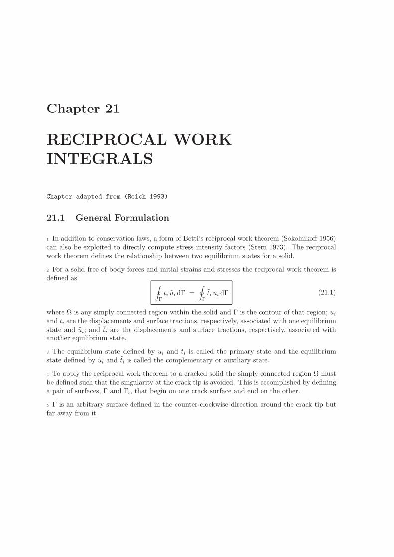
Chapter 21
RECIPROCAL WORKINTEGRALS
Chapter adapted from (Reich 1993)
21.1 General Formulation
1 In addition to conservation laws, a form of Betti’s reciprocal work theorem (Sokolnikoff 1956)can also be exploited to directly compute stress intensity factors (Stern 1973). The reciprocalwork theorem defines the relationship between two equilibrium states for a solid.
2 For a solid free of body forces and initial strains and stresses the reciprocal work theorem isdefined as ∮
Γti ui dΓ =
∮Γ
ti ui dΓ (21.1)
where Ω is any simply connected region within the solid and Γ is the contour of that region; ui
and ti are the displacements and surface tractions, respectively, associated with one equilibriumstate and ui; and ti are the displacements and surface tractions, respectively, associated withanother equilibrium state.
3 The equilibrium state defined by ui and ti is called the primary state and the equilibriumstate defined by ui and ti is called the complementary or auxiliary state.
4 To apply the reciprocal work theorem to a cracked solid the simply connected region Ω mustbe defined such that the singularity at the crack tip is avoided. This is accomplished by defininga pair of surfaces, Γ and Γε, that begin on one crack surface and end on the other.
5 Γ is an arbitrary surface defined in the counter-clockwise direction around the crack tip butfar away from it.

410 RECIPROCAL WORK INTEGRALS
6 Γε is a circle of radius ε centered on the crack tip that is defined in the clockwise directionaround the crack tip completely inside Γ.
7 Another pair of surfaces, Γ+t and Γ−
t , corresponding to the crack surfaces complete the defin-ition of Γ, as is shown in Figure 21.1. Γ+
t is defined on the upper crack surface between Γ andΓε and Γ−
t is defined on the lower crack surface bewteen Γε and Γ.
8 Naturally, Ω is the region inside this closed path through the solid. Since the material insideΓε is not included in the definition of Ω the singularity at the crack tip has been excluded.
Ω
cracktipcrack
x
y
surfaces
n
Γ
Γ
ε
Γ +
-Γ
t
t
εn
Figure 21.1: Contour integral paths around crack tip for recipcoal work integral
9 Assuming that Γ+t and Γ−
t are traction free the definition of the reciprocal work theorem canbe rewritten as∮
Γti ui dΓ =
∫Γ
ti ui dΓ +
∫Γε
ti ui dΓ =
∫Γ
ti ui dΓ +
∫Γε
ti ui dΓ (21.2)
in which the contributions from Γ and Γε are clearly separated.
10 This expanded expression is then rewritten in the form of Somigliana’s identity to obtain∫Γ(ti ui − ti ui) dΓ +
∫Γε
(ti ui − ti ui) dΓ = 0 (21.3)
11 The displacements ui and the stresses σij for the primary state can be decomposed into
ui = usi + ue
i + u0i
σij = σsij + σe
ij(21.4)
Victor Saouma Fracture Mechanics
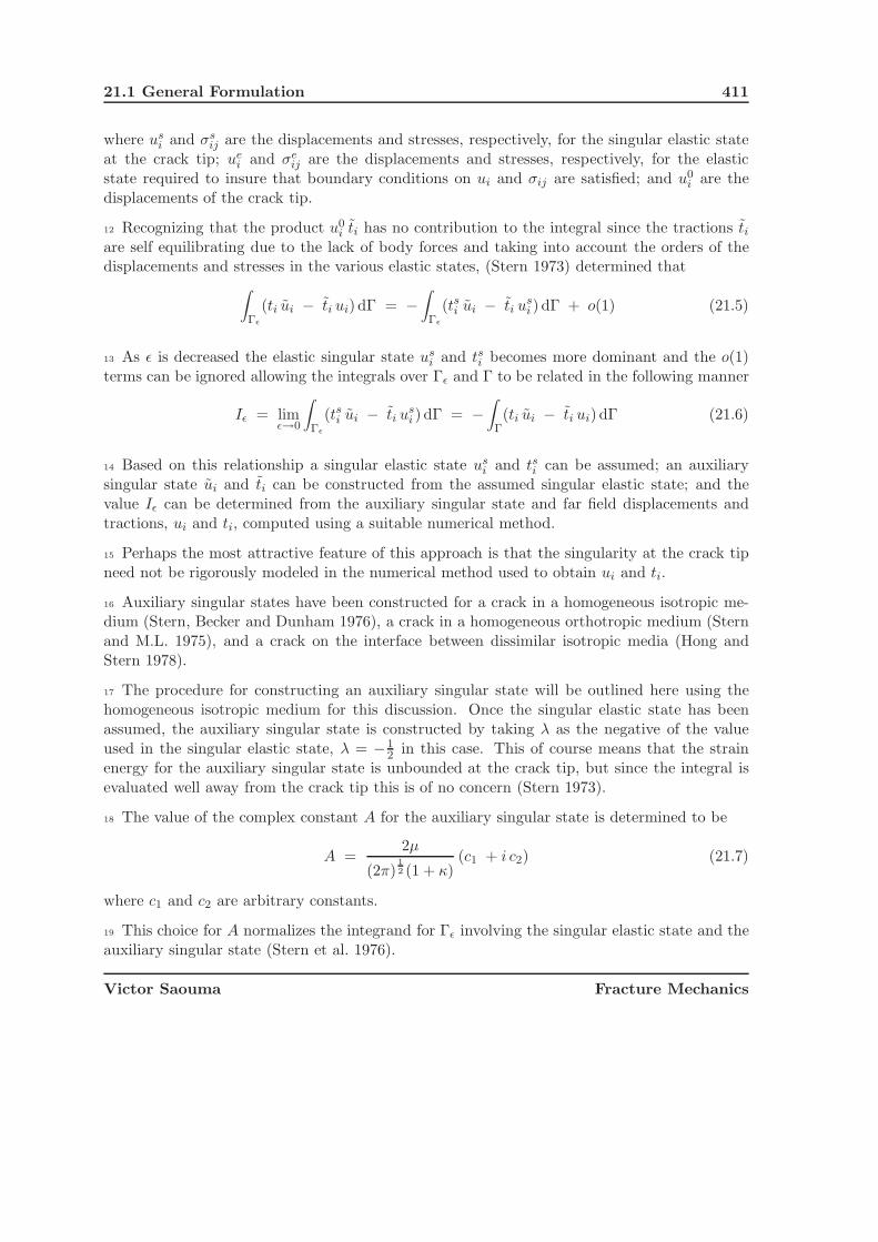
21.1 General Formulation 411
where usi and σs
ij are the displacements and stresses, respectively, for the singular elastic stateat the crack tip; ue
i and σeij are the displacements and stresses, respectively, for the elastic
state required to insure that boundary conditions on ui and σij are satisfied; and u0i are the
displacements of the crack tip.
12 Recognizing that the product u0i ti has no contribution to the integral since the tractions ti
are self equilibrating due to the lack of body forces and taking into account the orders of thedisplacements and stresses in the various elastic states, (Stern 1973) determined that∫
Γε
(ti ui − ti ui) dΓ = −∫Γε
(tsi ui − ti usi ) dΓ + o(1) (21.5)
13 As ε is decreased the elastic singular state usi and tsi becomes more dominant and the o(1)
terms can be ignored allowing the integrals over Γε and Γ to be related in the following manner
Iε = limε→0
∫Γε
(tsi ui − ti usi ) dΓ = −
∫Γ(ti ui − ti ui) dΓ (21.6)
14 Based on this relationship a singular elastic state usi and tsi can be assumed; an auxiliary
singular state ui and ti can be constructed from the assumed singular elastic state; and thevalue Iε can be determined from the auxiliary singular state and far field displacements andtractions, ui and ti, computed using a suitable numerical method.
15 Perhaps the most attractive feature of this approach is that the singularity at the crack tipneed not be rigorously modeled in the numerical method used to obtain ui and ti.
16 Auxiliary singular states have been constructed for a crack in a homogeneous isotropic me-dium (Stern, Becker and Dunham 1976), a crack in a homogeneous orthotropic medium (Sternand M.L. 1975), and a crack on the interface between dissimilar isotropic media (Hong andStern 1978).
17 The procedure for constructing an auxiliary singular state will be outlined here using thehomogeneous isotropic medium for this discussion. Once the singular elastic state has beenassumed, the auxiliary singular state is constructed by taking λ as the negative of the valueused in the singular elastic state, λ = −1
2 in this case. This of course means that the strainenergy for the auxiliary singular state is unbounded at the crack tip, but since the integral isevaluated well away from the crack tip this is of no concern (Stern 1973).
18 The value of the complex constant A for the auxiliary singular state is determined to be
A =2μ
(2π)12 (1 + κ)
(c1 + i c2) (21.7)
where c1 and c2 are arbitrary constants.
19 This choice for A normalizes the integrand for Γε involving the singular elastic state and theauxiliary singular state (Stern et al. 1976).
Victor Saouma Fracture Mechanics

412 RECIPROCAL WORK INTEGRALS
20 Having determined A, the product of this integral is
Iε = c1 KI + c2 KII + o(1) (21.8)
with the o(1) term going to zero as ε is decreased.
21 The stress intensity factors, KI and KII , can therefore be directly related to the integralover Γ
c1 KI + c2 KII =
∫Γ
[(ui − u0
i ) ti + ui ti]dΓ (21.9)
as was shown in Equation 21.6. When the integral is evaluated using ui and ti obtained fromthe numerical method the constants associated with the coefficients c1 and c2 are the stressintensity factors.
22 For the isotropic case, in the neighborhood of the crack tip, the displacements and thestresses, in polar coordinate system, are given by Westergaard as:
ur − u0r =
1
4μ
(r
2π
) 12{[
(2κ − 1) cosθ
2− cos
3θ
2
]KI
−[(2κ − 1) sin
θ
2− 3 sin
3θ
2
]KII
}+ O
(r
12
)(21.10)
uθ − u0θ =
1
4μ
(r
2π
) 12{[
−(2κ + 1) sinθ
2+ sin
3θ
2
]KI
−[(2κ + 1) cos
θ
2− 3 cos
3θ
2
]KII
}+ O
(r
12
)(21.11)
σr =1
4(2πr)12
{(5 cos
θ
2− cos
3θ
2
)KI −
(5 sin
θ
2− 3 sin
3θ
2
)KII
}+ O
(r−
12
)(21.12)
σθ =1
4(2πr)12
{(3 cos
θ
2+ cos
3θ
2
)KI −
(3 sin
θ
2+ 3 sin
3θ
2
)KII
}+ O
(r−
12
)(21.13)
σrθ =1
4(2πr)12
{(sin
θ
2+ sin
3θ
2
)KI +
(cos
θ
2+ 3 cos
3θ
2
)KII
}+ O
(r−
12
)(21.14)
where u0r and u0
θ are the radial and tangential components, respectively, of the displacementsu0 of the crack tip, and
KI = limr→0
(2πr)12 σθ|θ=0 (21.15)
KII = limr→0
(2πr)12 σrθ|θ=0 (21.16)
are the usual stress intensity factors.The auxiliary solution to be used in the reciprocal work relation is based on Williams
solution (Stern et al. 1976):
ur =1
2(2πr)12 (1 + κ){[
(2κ + 1) cos3θ
2− 3 cos
θ
2
]c1 +
[(2κ + 1) sin
3θ
2− sin
θ
2
]c2
}(21.17)
Victor Saouma Fracture Mechanics

21.1 General Formulation 413
uθ =1
2(2πr)12 (1 + κ){[
−(2κ − 1) sin3θ
2+ 3 sin
θ
2
]c1 +
[(2κ − 1) cos
3θ
2− cos
θ
2
]c2
}(21.18)
σr = − μ
2(2πr3)12 (1 + κ)
{[7 cos
3θ
2− 3 cos
θ
2
]c1 +
[7 sin
3θ
2− sin
θ
2
]c2
}(21.19)
σθ = − μ
2(2πr3)12 (1 + κ)
{[cos
3θ
2+ 3 cos
θ
2
]c1 +
[sin
3θ
2+ sin
θ
2
]c2
}(21.20)
σrθ = − μ
2(2πr3)12 (1 + κ)
{3
[sin
3θ
2+ sin
θ
2
]c1 −
[3 cos
3θ
2− cos
θ
2
]c2
}(21.21)
where c1 and c2 are arbitrary constants.
23 Now, on the inner circular boundary, the evaluation of the contour integral in terms oftraction and displacement takes the form:
Iε = −∫
Cε
((u − u0) · t) − u · t)ds
=
∫ π
−π[σr(ur − u0
r)σrθ(uθ − u0θ) − σrur + σrθuθ]rdθ (21.22)
24 When the two solutions are substituted into the preceding equation, we obtain:
Iε = c1KI − c2KII (21.23)
25 Thus it can be readily seen that Eq. ?? now reduces to:
c1KI − c2KII =
∫C
[(u− u0
)· t − u · t
]ds (21.24)
26 From this equation an algorithm for the SIF determination emerges:
1. Perform a linear elastic finite element analysis.
2. Extract u and t (displacements and traction) from the analysis.
3. Substitute into Eq. 21.24 along with the auxiliary solution.
4. The components of c1 in Eq. 21.24 yield KI .
5. The components of c2 in Eq. 21.24 yield KII .
Victor Saouma Fracture Mechanics

414 RECIPROCAL WORK INTEGRALS
27 In addition to demonstrating the reciprocal work integral for cracks in homogeneous isotropic(Stern et al. 1976), homogeneous orthotropic (Stern and M.L. 1975), and on the interfacebetween dissimilar isotropic materials (Hong and Stern 1978), Stern also proposed extensionsfor treating body forces (Stern et al. 1976) and thermal strains (Stern 1979). Unfortunately, thedescription of the extension for body forces was rather superficial, being limited to a footnote,and no example problems were presented for either of these extensions. However, for the caseof thermal strains it was clearly shown that there is no need to consider thermal loading inthe auxiliary state, meaning that the reciprocal work integral can also be extended includeinitial stresses without modifiying the auxiliary solution. More recent developments includethe treatment of dynamic crack propagation (Atkinson, Bastero and Miranda 1986, Bastero,Atkinson and Martinez-Esnaola 1989), sharp notches (Atkinson, Bastero and Martinez-Esnaola1988, Atkinson and Bastero 1991), and cracks in coupled poro-elastic media (Atkinson andCraster 1992).
21.2 Volume Form of the Reciprocal Work Integral
28 The first step to be taken when formulating extensions to the reciprocal work integral is thedefinition of the reciprocal work theorem accounting for the applied loads in the two equilibriumstates. Unfortunately, it is not always obvious how the reciprocal work theorem should bedefined to account for the applied loads, particularly when they are the result of initial strainsor stresses.
29 It will be shown here that the line integrals in the reciprocal work theorem can be convertedto volume integrals using Green’s theorem and that the form of the integrand for the volumeintegrals is such that the appropriate form of the reciprocal work theorem can be determinedquite simply.
30 (Sokolnikoff 1956) defined the reciprocal work theorem relating two separate equilibriumstates for a solid, both including body forces, as∫
Γti ui dΓ +
∫Ω
bi ui dΩ =
∫Γ
ti ui dΓ +
∫Ω
bi ui dΩ (21.25)
where ui, ti, and bi are the displacements, surface tractions, and body forces, respectively, forone equilibrium state; ui, ti, and bi are the displacements, surface tractions, and body forces,respectively, for the other equilibruim state; Ω corresponds to the volume of the solid; and Γcorresponds to the entire surface of the solid.
31 The equilibrium state defined by ui, ti, and bi is referred to as the primary state and theequilibrium state defined by ui, ti, and bi is referred to as the auxiliary state. Recalling fromthe equilibrium equation that bi = −σij,j and bi = −σij,j the reciprocal work theorem can berewritten as ∫
Γti ui dΓ −
∫Ω
σij,j ui dΩ =
∫Γ
ti ui dΓ −∫Ω
σij,j ui dΩ (21.26)
Victor Saouma Fracture Mechanics

21.3 Surface Tractions on Crack Surfaces 415
where σij and σij are the stress tensors for the two equilibrium states.
32 Adopting a counter-clockwise path around Γ the expressions relating dΓ to dx1 and dx2 givenin Equation ?? are still valid, allowing the line integrals to be written in a form compatiblewith Green’s theorem ∫
Γti ui dΓ =
∫Γ(−σi2 ui dx1 + σi1 ui dx2)∫
Γti ui dΓ =
∫Γ(−σi2 ui dx1 + σi1 ui dx2)
(21.27)
by expanding ti and ti in terms of σij , σij , and ni and collecting terms.
33 Applying Green’s theorem (Kreyszig 1979) to convert the line integrals to volume integralsyields ∫
Γti ui dΓ =
∫Ωσij,j ui dΩ +
∫Ωσij ui,j dΩ∫
Γti ui dΓ =
∫Ωσij,j ui dΩ +
∫Ωσij ui,j dΩ
(21.28)
and the reciprocal work theorem clearly simplifies to∫Ω
σij ui,j dΩ =
∫Ω
σij ui,j dΩ (21.29)
34 In the absence of body forces the volume integrals are not included in the definition ofthe reciprocal work theorem and the expression shown above is still valid since σij,j = 0 andσij,j = 0. Knowing that the line integral form of the reciprocal work theorem can be rewritten inthe volume integral form shown in Equation 21.29, the appropriate definition of the reciprocalwork theorem to account for initial strains and stresses in the primary state can be obtainedquite easily. This is accomplished by simply writing the volume form of the reciprocal worktheorem such that there is a direct relationship between the stresses and displacements in theprimary state.
21.3 Surface Tractions on Crack Surfaces
35 The extension to the reciprocal work integral to include the effect of surface tractions on thecrack surfaces in the primary state parallels the approach proposed by (Karlsson and Backlund1978) for the J integral.
36 For a primary state free of body forces with surface tractions on the crack surfaces thereciprocal work theorem is defined as∫
Γti ui dΓ =
∫Γ
ti ui dΓ (21.30)
Victor Saouma Fracture Mechanics

416 RECIPROCAL WORK INTEGRALS
37 This expression can be rewritten such that a separate integral is given for each portion ofthe contour path∫
Γti ui dΓ +
∫Γε
ti ui dΓ +
∫Γt
ti ui dΓ =
∫Γ
ti ui dΓ +
∫Γε
ti ui dΓ (21.31)
where Γt = Γ+t ∪ Γ−
t and ti is the applied surface traction vector on the crack surfaces in theprimary state.
38 This expression for the reciprocal work theorem can be rewritten in the form of Somigliana’sidentity as ∫
Γ(ti ui − ti ui) dΓ +
∫Γt
ti ui dΓ +
∫Γε
(ti ui − ti ui) dΓ = 0 (21.32)
39 Clearly, the integrand of the integral over Γε is identical to that for the case of a primarystate free of surface tractions on the crack surfaces, which means that Equation 21.5 still holdsand the solution for the auxiliary singular state is still valid.
40 The value Iε is then defined as
Iε = −∫Γ(ti ui − ti ui) dΓ − lim
ε→0
∫Γt
ti ui dΓ (21.33)
41 Provided that ti is not expressed in powers of r less than −12 , the limit exists and the stress
intensity factors are defined as
c1 KI + c2 KII =
∫Γ[ ti (ui − u0
i ) − ti ui] dΓ −∫Γt
ti ui dΓ (21.34)
where u0i are the displacements of the crack tip. However, when the integral over Γt is evaluated
using numerical integration techniques, quadratures based on sampling points that coincide withthe nodal locations should be avoided since ui is singular at the crack tip.
21.4 Body Forces
42 For a primary state with body forces but free surface tractions on the crack surfaces andinitial strains and stresses the reciprocal work theorem is defined as∫
Γti ui dΓ +
∫Ω
bi ui dΩ =
∫Γ
ti ui dΓ (21.35)
where bi is the body force vector. It should be noted that since the line integrals are definedover Γ this form of the reciprocal work integral could also account for surface tractions on thecrack surfaces.
Victor Saouma Fracture Mechanics

21.5 Initial Strains Corresponding to Thermal Loading 417
43 The expression for the reciprocal work theorem can be rewritten such that a separate integralis given for each portion of the contour path∫
Γti ui dΓ +
∫Γε
ti ui dΓ +
∫Ω
bi ui dΩ =
∫Γ
ti ui dΓ +
∫Γε
ti ui dΓ (21.36)
44 This expression can be rewritten in the form of Somigliana’s identity as∫Γ(ti ui − ti ui) dΓ +
∫Ω
bi ui dΩ +
∫Γε
(ti ui − ti ui) dΓ = 0 (21.37)
45 Clearly, the integrand of the integral over Γε is identical to that for the case of a primarystate free of body forces, which means that Equation 21.5 still holds and the solution for theauxiliary singular state described is still valid.
46 The value Iε is then defined as
Iε = −∫Γ(ti ui − ti ui) dΓ − lim
ε→0
∫Ω
bi ui dΩ (21.38)
Provided that bi is not expressed in powers of r less than −12 , the limit exists and the stress
intensity factors are defined as
c1 KI + c2 KII =
∫Γ[ ti (ui − u0
i ) − ti ui] dΓ −∫Ω
bi ui dΩ (21.39)
where u0i are the displacements of the crack tip. However, when the integral over Ω is evaluated
using numerical integration techniques, quadratures based on sampling points that coincidewith the nodal locations should be avoided since ui is singular at the crack tip.
21.5 Initial Strains Corresponding to Thermal Loading
47 For problems in thermo-elasticity the constitutive law defines net effective stresses σ′ij in
terms of the total strains εij and the thermal strains ε0ij , as is shown in Equation 21.53.
48 σ′ij can be decomposed into effective stresses σ′
ij and thermal stresses σ′′ij. σ′
ij are the resultof εij , which are, in turn, is defined by the displacements ui. Therefore, the effective stressesσ′
ij are then directly related to the displacements ui and should be used in the definition of thereciprocal work theorem rather than the net effective stresses σ′
ij .
49 The volume form of the reciprocal work theorem for a primary state that includes thermalstrains is ∫
Ωσ′
ij ui,j dΩ =
∫Ω
σij ui,j dΩ (21.40)
Victor Saouma Fracture Mechanics

418 RECIPROCAL WORK INTEGRALS
50 The relationship between the line and volume integral forms of the reciprocal work theoremcan be readily obtained by applying Green’s theorem to the volume integral with σ′
ij in theintegrand ∫
Γt′i ui dΓ =
∫Ω
σ′ij,j ui dΩ +
∫Ω
σ′ij ui,j dΩ (21.41)
where t′i = σ′ijnj is the effective surface traction vector.
51 Recalling from the equilibrium equation that σ′ij,j = αCijklT,jδkl in the absence of body
forces, it is clearly evident that a volume integral is required to complete the definition of thereciprocal work theorem.
52 Therefore, the appropriate form of the reciprocal work theorem for a primary state withthermal strains but no body forces is∫
Γt′i ui dΓ −
∫Ω
α (Cijkl T,i δkl)ui dΩ =
∫Γ
ti ui dΓ (21.42)
where T,i is the gradient of the temperatures.
53 A more general form of the reciprocal work theorem would be∫Γ
t′i ui dΓ +
∫Ω
b′i ui dΩ =
∫Γ
ti ui dΓ (21.43)
where b′i is the effective body force vector, as defined in Equation 21.58, which in this particularcase does not include a true body force vector bi.
54 Recalling that the natural boundary conditions are defined in terms of the total stresses,t′i �= 0 on the crack surfaces. Therefore, the form of the reciprocal work theorem in which theline integrals on Γ have been separated is∫
Γt′i ui dΓ +
∫Γε
t′i ui dΓ +
∫Γt
t′i ui dΓ +
∫Ω
b′i ui dΩ =
∫Γ
ti ui dΓ +
∫Γε
ti ui dΓ (21.44)
where t′i is the applied effective surface traction vector, as defined in Equation 21.60, which,much like the effective body force vector b′i, does not include a true applied surface tractionvector in this case.
55 This expression for the reciprocal work theorem can be rewritten in the form of Somigliana’sidentity as∫
Γ(t′i ui − ti ui) dΓ +
∫Γt
t′i ui dΓ +
∫Ω
b′i ui dΩ +
∫Γε
(t′i ui − ti ui) dΓ = 0 (21.45)
56 Clearly, the integrand of the integral over Γε is identical to that for the case of a primarystate free of initial strains, which means that Equation 21.5 still holds and the solution for theauxiliary singular state described in Section ?? is still valid.
Victor Saouma Fracture Mechanics

21.6 Initial Stresses Corresponding to Pore Pressures 419
57 The value Iε is then defined as
Iε = −∫Γ(t′i ui − ti ui) dΓ − lim
ε→0
∫Γt
t′i ui dΓ − limε→0
∫Ω
b′i ui dΩ (21.46)
Provided that the temperature T is not expressed in powers of r less than 12 , the limit exists
and the stress intensity factors are defined as
c1 KI + c2 KII =
∫Γ[ ti (ui − u0
i ) − t′i ui] dΓ −∫Γt
t′i ui dΓ −∫Ω
b′i ui dΩ (21.47)
where u0i are the displacements of the crack tip.
58 However, when the integrals over Γt and Ω are evaluated using numerical integration tech-niques, quadratures based on sampling points that coincide with the nodal locations should beavoided since ui is singular at the crack tip.
21.6 Initial Stresses Corresponding to Pore Pressures
59 The stress-strain relationship for poro-elasticity, which is obtained by substituting the con-stitutive law defining the effective stresses σ′
ij into the principle of effective stress, defines thetotal stresses σij in terms of the total strains εij and the pore pressures p, as was shown inEquation 21.62.
60 As was the case for problems in thermo-elasticity, σij can again be decomposed, but in thisinstance the constituent stresses are σ′
ij and the initial stresses σ0ij corresponding to the pore
pressures. Since εij is defined in terms of the displacements ui, the effective stresses σ′ij are
then directly related to the displacements ui and the reciprocal work theorem is again definedin terms of the effective stresses in the primary state.
61 Therefore, Equations 21.40 and 21.41 also apply when the primary state includes initialstresses. Recalling from the equilibrium equation that σ′
ij,j = p,jδij in the absence of bodyforces, it is clearly evident that a volume integral is required to complete the definition of thereciprocal work theorem.
62 Therefore, the appropriate form of the reciprocal work theorem for a primary state with porepressures but no body forces is∫
Γt′i ui dΓ −
∫Ω
p,i ui dΩ =
∫Γ
ti ui dΓ (21.48)
where p,i is the gradient of the pore pressures.
63 A more general form of the reciprocal work integral is∫Γ
t′i ui dΓ +
∫Ω
b′i ui dΩ =
∫Γ
ti ui dΓ (21.49)
Victor Saouma Fracture Mechanics

420 RECIPROCAL WORK INTEGRALS
where b′i is the effective body force vector, as defined in Equation 21.64, which does not includea true body force vector bi in this case.
64 Recognizing that the general form of the reciprocal work theorem accounting for initialstresses is identical to that accounting for initial strains (i.e. Equation 21.43), Equations 21.44through 21.47 apply for initial stresses as well. However, the applied effective surface tractionvector is defined by Equation 21.65 and the pore pressure p rather than the temperature Tmust be expressed in a power of r greater than 1
2 in order for the limits in Equation 21.46 toexist. Naturally, the restrictions on the choice of numerical integration techniques are also stillin effect.
21.7 Combined Thermal Strains and Pore Pressures
65 Recalling that in the absence of initial strains and stresses that the total stresses σij andthe effective stresses σ′
ij are equivalent, it is quite clear that Equation 21.43 also defines thereciprocal work theorem for solids that are free of initial strains and stresses.
66 Due to the general definitions of the applied effective surface traction vector t′i and theeffective body force vector b′i, the cases of a primary state with true surface tractions ti on thecrack surfaces and true body forces bi are also addressed by Equation 21.43.
67 Therefore, the stress intensity factors for a primary state which includes any combination ofsurface tractions on the crack surfaces, body forces, and initial strains and stresses are definedby Equation 21.47. The relationship between the stress intensity factors and the reciprocalwork theorem is obtained by substituting the expressions for t′i and b′i defined by Equation21.69 into Equation 21.47
c1 KI + c2 KII =
∫Γ[ ti (ui − u0
i ) − (ti + p ni + α T Cijkl ni δkl) ui] dΓ
−∫Γt
(ti + p ni + α T Cijkl ni δkl) ui dΓ
−∫Ω(bi − p,i − α Cijkl Ti δkl) ui dΩ (21.50)
68 Naturally, the restrictions imposed on the power of r for ti, bi, T , and p are still in effect, asare the restrictions on the choice of numerical integration techniques.
21.8 Field Equations for Thermo- and Poro-Elasticity
69 In thermo or poro-elasticity the thermal strains and pore pressures are usually treated asinitial strains and initial stresses, respectively.
Victor Saouma Fracture Mechanics

21.8 Field Equations for Thermo- and Poro-Elasticity 421
70 The general stress-strain relationship obtained by substituting the constutive law into theeffective stress principle is
σij = Cijkl (εkl − ε0kl) + σ0
ij (21.51)
71 Clearly, in the absence of initial stresses σij = σ′ij and in the absence of both initial strains
and stresses σij = σ′ij.
72 The thermal strains for an isotropic material are defined in terms of the temperature T andthe coefficient of thermal expansion α as
ε0ij = α T δij (21.52)
where δij is the Kronecker delta. Substituting this expression for the thermal strains intoEquation 21.51, the resulting constitutive law for thermo-elasticity is
σ′ij = Cijkl (εkl − αT δkl) (21.53)
73 The thermal stresses σ′′ij are defined as
σ′′ij = α T Cijkl δkl (21.54)
and the net strains Eij are defined as
Eij = εkl − αT δkl (21.55)
74 Adopting the standard form of the effective stress principle the equilibrium equation andnatural boundary conditions, respectively, can be rewritten in terms of the effective stresses
σ′ij,j + b′i = 0
σ′ij nj − t′i = 0
(21.56)
where b′i is the effective body force vector and t′i is the applied effective surface traction vector.
75 The effective body force vector b′i is defined as
b′i = bi − σ′′ij,j (21.57)
and may be rewritten in terms of the temperature gradient vector T,i
b′i = bi − αCijkl T,i δkl (21.58)
based on the definition of the thermal stresses given in Equation 21.54 and the assumption ofa homogeneous material.
76 The applied effective surface traction vector t′i is defined as
t′i = ti + σ′′ij nj (21.59)
Victor Saouma Fracture Mechanics

422 RECIPROCAL WORK INTEGRALS
and may be rewritten in terms of the temperature T
t′i = ti + α T Cijkl ni δkl (21.60)
based on the definition of the thermal stresses given in Equation 21.54.
77 Pore pressures are typically defined using the sign convention for soil mechanics in whichcompression is positive, but in the sign convention for standard solid mechanics tension isconsidered to be positive. Therefore, the initial stresses corresponding to a pore pressure aredefined as
σ0ij = −p δij (21.61)
where p is the pore pressure defined using the compression positive sign convention; the minussign corrects the discrepancy in the sign conventions; and δij is the Kronecker delta. In theclassical interpretation of the behavior of a porous material (Terzaghi and Peck 1967), thepore pressures p act only in the voids of the material and the effective stresses act only on theskeleton of the material.
78 It must be noted that the pore pressures p being considered in this discussion and throughoutthe remainder of this chapter are the steady state pore pressures; excess pore pressures resultingfrom dilatant behavior in the skeleton of the material are not considered.
79 The stress-strain relationship for poro-elasticity
σij = Cijkl εkl − p δij (21.62)
is obtained by substituting the expression for the initial stresses into Equation 21.51.
80 Adopting the standard form of the principle of effective stress the equilibrium equation andthe natural boundary conditions, respectively, can be rewritten in terms of the effective stresses
σ′ij,j + b′i = 0
σ′ij nj − t′i = 0
(21.63)
where b′i is the effective body force vector and t′i is the applied effective surface traction vector.
81 The effective body force vector b′i is defined as
b′i = bi − p,i (21.64)
where p,i is the pore pressure gradient vector. The applied effective surface traction vector t′iis defined as
t′i = ti + p ni (21.65)
82 Since σ′ij = 0 on surfaces exposed to hydrostatic pressures but no other surface tractions,
ti = −p ni on these surfaces.
Victor Saouma Fracture Mechanics

21.8 Field Equations for Thermo- and Poro-Elasticity 423
83 When thermal strains and pore pressures are considered in combination the constitutive lawis defined as a simple combination of Equations 21.53 and 21.62
σij = Cijkl (εkl − α T δkl) − p δij (21.66)
84 The equilibrium equation and natural boundary conditions, respectively, can be rewritten interms of either the effective stresses σ′
ij
σ′ij,j + b′i = 0
σ′ij nj − t′i = 0
(21.67)
or the net effective stresses σ′ij
σ′ij,j + b′i = 0
σ′ij nj − t′i = 0
(21.68)
85 The field equations defined in terms of σ′ij are obtained by adopting the standard form of the
principle effective stress and the field equations defined in terms of σ′ij are obtained by adopting
the alternate form of the principle effective stress.
86 When the equilibrium equation and natural boundary conditions are written in terms of σ′ij
the effective body forces b′i and applied effective surface tractions t′i are defined as
b′i = bi − p,i − α Cijkl T,i δkl
t′i = ti + p ni + α T Cijkl ni δkl(21.69)
87 However, when the equilibrium equation and natural boundary conditions are written interms of σ′
ij the effective body forces b′i and applied effective surface tractions t′i are identicalto those for poro-elasticity (i.e. Equations 21.64 and 21.65, respectively).
Victor Saouma Fracture Mechanics

424 RECIPROCAL WORK INTEGRALS
Victor Saouma Fracture Mechanics
Chapter 22
FICTITIOUS CRACK MODEL
Originally published as:
Implementation and Validation of a nonlinear fracture model in a 2D/3D finite elementcode by Reich, Plizzari, Cervenka and Saouma; in Numerical Models in Fracture of Concrete;Wittman Ed., Balkema (1993).
1 An incremental formulation for the Fictitious Crack Model (FCM) will be presented. Thecomputational algorithm treats the structure as a set of sub-domains bonded along assumedcrack paths. The crack paths are defined by interface elements that initially act as constraintsenforcing the bond between adjacent sub-domains, but change state to function as standardinterface elements as the crack propagates. Constraints are enforced on the global system ofequations using a penalty approach.
2 A load scaling strategy, which allows for load controlled analyses in the post-peak regime, isused to enforce stress continuity at the tip of the Fracture Process Zone (FPZ).
3 To demonstrate the accuracy of the computational algorithm, a series of three wedge-splitting(WS) test specimens are analyzed. Specimen sizes are 31, 91, and 152 cm (1, 3, and 5 ft).Material properties for the concrete are taken as the mean values of the observed experimentalresults for all specimen sizes. The computed results are compared to the envelopes of theexperimental response for each specimen size.
22.1 Introduction
4 The most commonly implemented nonlinear fracture model for concrete using the discretecrack approach is the FCM (Hillerborg, A. and Modeer, M. and Petersson, P.E. 1976a). Inthe FCM the zone of micro-cracking and debonding ahead of the crack front is modeled as acohesive stress that acts to close the crack. The magnitude of the cohesive stresses on the crack

426 FICTITIOUS CRACK MODEL
surface are determined by a softening law that relates the stress to the relative displacement ofthe crack surfaces through the fracture energy.
5 Many implementations of the FCM have been reported (Ingraffea and Gerstle 1984, Roelfstraand Sadouki 1986, Dahlblom and Ottosen 1990, Bocca, Carpinteri and Valente 1990, Gopalarat-nam and Ye 1991, Gerstle and Xie 1992), but none of the implementations based on a discretecrack approach claim to be based on the standard incremental formulation normally associatedwith nonlinear analyses. Only the implementation by Dahlbom and Ottosen (Dahlblom andOttosen 1990), which is based on a smeared crack approach, uses an incremental formulation.
6 In this chapter, an incremental solution algorithm for the FCM based in the discrete crackapproach will be presented and its performance evaluated by comparing the computed responseof WS test specimens against known experimental results.
22.2 Computational Algorithm
7 Treatment of the structure as a set of bonded sub-domains results in a system of mixedequations with the unknowns being displacements and surface tractions on the interface betweenthe sub-domains. The weak form of the system of mixed equations will be derived from thePrinciple of Virtual Work. The weak form equations will then be discretized for solution usingthe finite element method. The penalty method solution for the mixed system of equationswill be discussed; particularly the automatic selection of the penalty number. Finally, anincremental-iterative solution strategy based on the modified-Newton algorithm that includesload scaling and allows for load control in the post-peak regime will be discussed.
22.2.1 Weak Form of Governing Equations
8 Figure 22.1 shows a body consisting of two sub-domains, Ω1 and Ω2 that intersect on a surfaceΓI without penetration. Each sub-domain may be subject to body forces bm or to prescribedsurface tractions tm on Γtm . Defining the volume of the body as
Ω = Ω1 ∪ Ω2 (22.1)
and the surface of the body subject to prescribed surface tractions as
Γt = Γt1 ∪ Γt2 , (22.2)
the Principle of Virtual Work for the body is∫Ω
δεTσdΩ −
∫Ω
δuT bdΩ −∫Γt
δuT tdΓ = 0 (22.3)
where
δε = Lδu (22.4-a)
ε = Lu (22.4-b)
σ = Dε (22.4-c)
Victor Saouma Fracture Mechanics

22.2 Computational Algorithm 427
Ω
Ω
Γ
Γ
Γ
Γ
Γ
Γt
u
t
u
I
I
1
2
t
t
b
c
1
1
2
2
2
1
Figure 22.1: Body Consisting of Two Sub-domains
9 Within each sub-domain of the body Ωm the Principle of Virtual Work must also hold, butadditional integrals are required to account for the work performed by the surface tractions tIm
on the interface ΓI . Surface tractions on the interface are due to bonding of the sub-domainstbm
or to cohesive stresses in the FPZ tcm. In either case, stress continuity on ΓI requires that
tb2 = −tb1 (22.5-a)
tc2 = −tc1 (22.5-b)
10 Defining the interface surface asΓI = ΓIb
∪ ΓIc , (22.6)
where ΓIbis the bonded interface surface and ΓIc is the interface surface subject to cohesive
stresses, the external work on the interface is written as∫ΓI
δuT1 tI1dΓ =
∫ΓIb
δuT1 tbdΓ +
∫ΓIc
δuT1 tcdΓ (22.7-a)∫
ΓI
δuT2 tI2dΓ = −
∫ΓIb
δuT2 tbdΓ −
∫ΓIc
δuT2 tcdΓ (22.7-b)
Both tb and tc are unknown, but as tb acts on the bonded, or constrained, interface it will betreated as a Lagrange multiplier
λ = tb (22.8)
Victor Saouma Fracture Mechanics

428 FICTITIOUS CRACK MODEL
11 Substituting λ into Equations 22.3 and 22.4-a-22.4-c and including the external work per-formed by the surface tractions on the interface surface, the Principle of Virtual Work forsub-domains Ω1 and Ω2 is written as∫
Ω1
δεT1 σ1dΩ −
∫Ω1
δuT1 b1dΩ −
∫Γt1
δuT1 t1dΓ −
∫ΓIb
δuT1 λdΓ −
∫ΓIc
δuT1 tcdΓ = 0∫
Ω2
δεT2 σ2dΩ −
∫Ω2
δuT2 b2dΩ −
∫Γt2
δuT2 t2dΓ +
∫ΓIb
δuT2 λdΓ +
∫ΓIc
δuT2 tcdΓ = 0
(22.9)
12 On ΓIbthe displacements for the two sub-domains, u1 |ΓIb
and u2 |ΓIb, must be equal. This
condition can be written as a constraint in the strong form
u2 |ΓIb−u1 |ΓIb
= 0, (22.10)
but a weak form is required to be compatible with Equation 22.5-a-22.5-b. The following weakform ∫
Γi
δλT (u2 − u1)dΓ = 0 (22.11)
was chosen for the constraint equation as it makes the system of mixed equations symmetric.
22.2.2 Discretization of Governing Equations
13 Discretization of Equations 22.9-22.9 and 22.11 will be presented as if each sub-domainwere an element (Zienkiewicz and Taylor 1989); the extension to multi-element sub-domains isstraightforward and will be omitted from this discussion. Each sub-domain Ωm is discretizedfor displacements um such that nodes on Γtm and ΓI are included in the vector of discretedisplacements um. The number of nodes on ΓI in Ω1 is equal to the number of nodes on ΓI inΩ2. For each node on ΓI in Ω1 there is a node on ΓI in Ω2 with the same coordinates. Thenodes at which the surface tractions due to bonding λ on ΓIb
are discretized are at the samelocations as those for the displacements.
14 Displacements um within the sub-domains Ωm and the surface tractions λ on the bondedinterface ΓIb
are defined in terms of their discretized counterparts using shape functions
um = Numum (22.12-a)
λ = Nλλ (22.12-b)
δum = Numδum (22.12-c)
δλ = Nλδλ (22.12-d)
Num and Nλ are standard shape functions in that for each node there is a correspondingshape function whose value is one at that node and zero at all other nodes.
Victor Saouma Fracture Mechanics
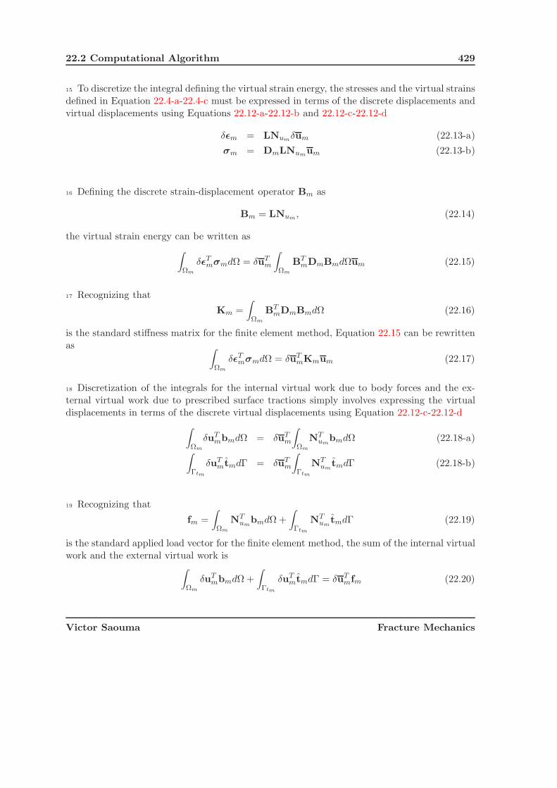
22.2 Computational Algorithm 429
15 To discretize the integral defining the virtual strain energy, the stresses and the virtual strainsdefined in Equation 22.4-a-22.4-c must be expressed in terms of the discrete displacements andvirtual displacements using Equations 22.12-a-22.12-b and 22.12-c-22.12-d
δεm = LNumδum (22.13-a)
σm = DmLNumum (22.13-b)
16 Defining the discrete strain-displacement operator Bm as
Bm = LNum, (22.14)
the virtual strain energy can be written as∫Ωm
δεTmσmdΩ = δuT
m
∫Ωm
BTmDmBmdΩum (22.15)
17 Recognizing that
Km =
∫Ωm
BTmDmBmdΩ (22.16)
is the standard stiffness matrix for the finite element method, Equation 22.15 can be rewrittenas ∫
Ωm
δεTmσmdΩ = δuT
mKmum (22.17)
18 Discretization of the integrals for the internal virtual work due to body forces and the ex-ternal virtual work due to prescribed surface tractions simply involves expressing the virtualdisplacements in terms of the discrete virtual displacements using Equation 22.12-c-22.12-d∫
Ωm
δuTmbmdΩ = δuT
m
∫Ωm
NTum
bmdΩ (22.18-a)∫Γtm
δuTmtmdΓ = δuT
m
∫Γtm
NTum
tmdΓ (22.18-b)
19 Recognizing that
fm =
∫Ωm
NTum
bmdΩ +
∫Γtm
NTum
tmdΓ (22.19)
is the standard applied load vector for the finite element method, the sum of the internal virtualwork and the external virtual work is∫
Ωm
δuTmbmdΩ +
∫Γtm
δuTmtmdΓ = δuT
mfm (22.20)
Victor Saouma Fracture Mechanics

430 FICTITIOUS CRACK MODEL
20 To discretize the external virtual work due to surface tractions on the interface, the surfacetractions and the virtual displacements must be expressed in terms of the discrete surfacetractions and virtual displacements using Equations 22.12-a-22.12-b and 22.12-c-22.12-d∫
ΓIb
δuTmλdΓ = δuT
m
∫ΓIb
NTum
NλdΓλ (22.21-a)∫Γtc
δuTmtcdΓ = δuT
m
∫Γtc
NTum
tcdΓ (22.21-b)
21 Defining the operator matrix for the load vector due to surface tractions on the bondedinterface as
Qm =
∫ΓIb
NTum
NλdΓ (22.22)
and the load vector for the cohesive stresses as
fcm =
∫Γtc
NTum
tcdΓ (22.23)
the external work due to surface tractions on the interface is∫ΓIb
δuTmλdΓ +
∫Γtc
δuTmtcdΓ = δuT
m(Qmλ + fcm) (22.24)
22 To discretize the weak constraint equation, the displacements and the virtual surface trac-tions must be expressed in terms of the discrete displacements and the discrete virtual surfacetractions using Equations 22.12-a-22.12-b and 22.12-c-22.12-d∫
ΓIb
δλTu1dΓ = δλT∫ΓIb
NTλNu1dΓu1 (22.25-a)∫
ΓIb
δλTu2dΓ = δλT∫ΓIb
NTλNu2dΓu2 (22.25-b)
23 Recognizing that
QTm =
∫ΓIb
NTλNumdΓ (22.26)
is the transpose of the operator matrix for the load vector due to surface tractions on thebonded interface defined in Equation 22.23, the weak constraint equation can be rewritten as∫
ΓIb
δλT (u2 − u1)dΓ = δλT(QT
2 u2 − QT1 u1) = 0 (22.27)
24 Having defined the discretized form of all integrals in the governing equations, it is nowpossible to define the discrete system of mixed equations. Substituting Equations 22.17, 22.20,
Victor Saouma Fracture Mechanics

22.2 Computational Algorithm 431
and 22.24 into Equation 22.9-22.9 and rearranging terms, the discrete Principle of Virtual Workis written as
δuT1 (K1u1 − Q1λ) = δuT
1 (f1 + fc1) (22.28-a)
δuT2 (K2u2 + Q2λ) = δuT
2 (f2 − fc2) (22.28-b)
25 As δuTm appears in both sides of Equation 22.28-a-22.28-b, it can be eliminated, leaving
K1u1 − Q1λ = f1 + fc1 (22.29-a)
K2u2 + Q2λ = f2 − fc2 (22.29-b)
26 In a similar fashion, δλT
can be eliminated from Equation 22.27, leaving
QT2 u2 − QT
1 u1 = 0 (22.30)
as the discrete constraint equation. The discrete system of mixed equations is defined byEquations 22.29-a-22.29-b and 22.30, which can be written in matrix form as⎡
⎢⎣ K1 0 −Q1
0 K2 Q2
−QT1 QT
2 0
⎤⎥⎦⎧⎪⎨⎪⎩
u1
u2
λ
⎫⎪⎬⎪⎭ =
⎧⎪⎨⎪⎩
f1 + fc1f2 − fc2
0
⎫⎪⎬⎪⎭ (22.31)
22.2.3 Penalty Method Solution
27 The penalty method (Zienkiewicz and Taylor 1989) was chosen for the solution of the discretesystem of mixed equations because it reduces the problem to that of a single-field. Reducingthe system of mixed equations to a single-field equation decreases the number of unknowns thatmust be solved for and simplifies the use of direct solution methods.
28 Direct solution methods can be used with the system of mixed equations, but interlacingof the equations is required to avoid singularities (Wiberg 1974). Another troublesome aspectrelated to the use of direct solution methods with the system of mixed equations is that sincecrack propagation is simulated by the release of constraints on the interface, the total numberof unknowns would change as the crack propagates. Interlacing a system of mixed equationswith an ever changing number of unknowns would certainly create major bookkeeping problemsin a finite element code.
29 To obtain the penalty form of the system of mixed equations, Equation 22.31 is rewritten as⎡⎢⎣ K1 0 −Q1
0 K2 Q2
−QT1 QT
2 − 1αI
⎤⎥⎦⎧⎪⎨⎪⎩
u1
u2
λ
⎫⎪⎬⎪⎭ =
⎧⎪⎨⎪⎩
f1 + fc1f2 − fc2
0
⎫⎪⎬⎪⎭ (22.32)
Victor Saouma Fracture Mechanics

432 FICTITIOUS CRACK MODEL
where α is the penalty number. α should be sufficiently large that 1αI is close to zero. It is now
possible to express λ in terms of u1 and u2
λ = α(Q2u2 − Q1u1) (22.33)
30 Substituting Equation 22.33 into Equation 22.32, a single-field penalized stiffness matrixequation is obtained
[(K1 + αQ1Q
T1 ) −αQ1Q
T2
−αQ2QT1 (K2 + αQ2Q
T2 )
]{u1
u2
}=
{f1 + fc1f2 − fc2
}(22.34)
31 The selection of a good penalty number is a rather difficult task. If the penalty numberis too small the computed displacements will yield a substantial error when inserted into theconstraint equation
Q2u2 − Q1u1 = ε � 0 (22.35)
32 As the penalty number is increased the error ε approaches zero, but the character of thesystem of equations changes as the effect of K1 and K2 is diminished. When the effect of K1
and K2 is significantly diminished the computed displacements away from the interface, whichare not included in the constraint equation, will lose accuracy due to round off errors. The goalis to select a penalty number that yields an acceptable error when the computed displacementsare inserted in the constraint equation without sacrificing the accuracy of the displacementsaway from the interface. The author’s experience is that a penalty number selected using
α =max(diag(Km))
max(diag(QmQTm))
× 106 (22.36)
yields very good results for the class of problems being considered.
33 Penalty numbers selected in this fashion result in computed values of u1 and u2 on theinterface that tend to be identical for the first five or six digits when the penalized stiffnessmatrix is assembled in double precision.
22.2.4 Incremental-Iterative Solution Strategy
34 An incremental-iterative solution strategy is used to obtain the equilibrium configurationfor each crack length. At zero load, the entire interface is constrained (i.e., fully bonded). Asload is applied, surface tractions on the constrained interface violate a strength criteria andthe corresponding constraints are released. On that portion of the interface where constraintshave been released, cohesive stresses act until the relative displacements of the unconstrainedinterface surfaces become large enough to dictate otherwise.
35 In this solution strategy crack propagation occurs after every increment.
Victor Saouma Fracture Mechanics

22.2 Computational Algorithm 433
36 The use of a strength criteria to detect the onset of crack propagation requires that themagnitude of the applied loads be such that the surface tractions at a node on the constrainedinterface are precisely equal to the maximum allowable stress. In this case, equality is requiredbetween the normal surface traction and the uniaxial tensile strength. However, as the magni-tude of the applied loads that causes the strength criteria to be satisfied exactly is not knowna priori, some form of automatic load scaling must be included in the solution strategy.
37 Assuming that the applied loads are proportional, a load factor β can be used to scale anarbitrary set of applied load vector f of some arbitrary magnitude. At the beginning of eachload increment i, the load factor is βi and the applied load vector is
βif = βi
{f1f2
}(22.37)
The value of βi is zero at the beginning of the first increment. The incremental load factor forincrement i is Δβi and the applied incremental load vector is
Δβif = Δβi
{f1f2
}(22.38)
The load factor at the end of increment i is
βi+1 = βi + Δβi (22.39)
38 The modified-Newton algorithm (Zienkiewicz and Taylor 1991) is used to solve for incremen-tal displacements due to the applied incremental loads. The incremental displacements for ageneric increment are defined as
Δun+1 = Δun + δun (22.40)
where
u =
{u1
u2
}(22.41)
and Δun is the incremental displacement vector at the beginning of iteration n and δun is thecorrection to the incremental displacement vector for iteration n.
39 In a similar fashion, the incremental load factor is defined as
Δβn+1 = Δβn + δβn (22.42)
where Δβn is the incremental load factor at the beginning of iteration n and δβn is the correctionto the incremental load factor for iteration n. At the beginning of the first iteration both Δun
and Δβn are zero.
40 Displacement corrections are computed by solving
Kαdun = (βf + Δβnf + dβnf + fnc − pn) (22.43)
Victor Saouma Fracture Mechanics
434 FICTITIOUS CRACK MODEL
where
Kα =
[(K1 + αQ1Q
T1 ) −αQ1Q
T2
−αQ2QT1 (K2 + αQ2Q
T2 )
](22.44)
is the penalized stiffness matrix;
fnc =
{fnc1
−fnc2
}(22.45)
is the load vector due to cohesive stresses on the interface at the beginning of iteration n; and
pn =nelem∑i=1
∫Ωei
BTD(ε + Δεn)dΩ (22.46)
is the reaction vector for the state of stress at iteration n.
41 Recognizing thatrn = βf + Δβnf + fn
c − pn (22.47)
is the residual force vector at the beginning of iteration n, Equation 22.43 can be written in amore compact fashion as
dun = K−1α (δβnf + rn) (22.48)
42 Since the K−1α f term does not change throughout the course of the iterative process it can
be defined as a constant value for the increment
δuT = K−1α f (22.49)
43 The displacement vector δuT is commonly called the tangent displacement vector (Crisfield,M.A. 1981). At this point, the iterative displacement correction can be defined as
δun = δβnδuT + K−1α rn (22.50)
44 Having shown how the load factor is implemented within the incremental-iterative solutionstrategy, the last detail left to explain is the procedure for computing δβn such that the strengthcriteria is exactly satisfied. Since the surface tractions on the constrained interface are used todetermine the magnitude of the applied load, the total surface tractions for iteration n must beexpressed in terms of its various contributions
λn+1
= λ + Δλn
+ δλnr + δβnδλT (22.51)
where λ is the surface traction vector at the beginning of the increment; Δλn
is the incrementalsurface traction vector at the beginning of iteration n; δλ
nr is correction to the incremental
Victor Saouma Fracture Mechanics

22.3 Validation 435
surface traction vector due to the residual load vector rn for iteration n; and δλT is the surfacetraction vector due to the tangent displacement vector δuT . δλ
nr and δλT are defined as
δλnr = α(QT
2 δunr2
− QT1 δun
r1) (22.52-a)
δλT = α(QT2 δuT − QT
1 δuT ) (22.52-b)
45 The strength criteria is applied to λn+1
on a node-by-node basis such that
max((λn+1
)i(n)i) = ft (22.53)
where (n)i is the normal vector at node i and ft is the uniaxial tensile strength.
46 Recognizing that λ, Δλn, and δλ
nr are fixed for iteration n, the iterative load factor correction
is defined as
δβn = min
⎧⎨⎩
ft −[(λ)i + (Δλ
n)i + (δλ
nr )i](n)i
(δλT )i(n)i
⎫⎬⎭ (22.54)
Provided that the cohesive stresses on the interface are treated as forces and no stiffness matrixis assembled for those interface elements, this solution strategy allows for load control in thepost peak regime.
47 The use of stiffness matrices for the interface elements subject to softening is avoided becausetheir presence in the global stiffness matrix will eventually cause it to become non-positivedefinite.
22.3 Validation
48 In order to assess the algorithm just presented, analysis of previously tested wedge-splittingtest specimens was undertaken, Fig. 22.2. In those tests, described in (Saouma, Broz, Bruhwilerand Boggs 1991), wedge-splitting specimens of 31, 91, and 152 cm (1, 3, and 5 ft) with maximumaggregate sizes ranging from 19, 38, and 76 mm (0.75, 1.5, and 3 in) were tested under crackmouth opening displacement control.
22.3.1 Load-CMOD
49 The selected material properties were the average values reported in (Saouma, Broz, Bruhwilerand Boggs 1991) for the three specimen sizes with the 38 mm maximum aggregate size con-crete. In order to facilitate the use of Merlin (Saouma et al. 1997–2004) by practicing engineers,input prameters were intentionally kept to a minimum, and included: 1) Young’s modulus E,2) Poisson’s ratio ν, 3) tensile strength f ′
t; and 3) fracture energy GF . The tensile strength
Victor Saouma Fracture Mechanics

436 FICTITIOUS CRACK MODEL
Figure 22.2: Wedge Splitting Test, and FE Discretization
Victor Saouma Fracture Mechanics

22.3 Validation 437
f ′t was taken as 0.9f ′
c, and a bilinear curve for the softening behavior was systematically used
with the inflection point defined by s1 =f ′
t
4 , w1 = 0.75GF
f ′
t, and w2 = 5GF
f ′
tas recommended in
(Wittmann et al. 1988).
50 For each analysis, numerical predictions are shown in comparison with the range of experi-mental results, Figure 22.3.
51 From these figures, it can be readily observed that very good engineering comparaison isachieved between numerical predictions and experimental results.
52 Also shown are the results of an analysis of a hypothetical 50 ft specimen, which is a scaledup version of the 5 ft specimen. Material properties are the same as used for the precedinganalyses.
22.3.2 Real, Fictitious, and Effective Crack Lengths
53 For each of the preceding analysis, the lengths of the real, fictitious and effective crackswere determined. Whereas the first two are directly obtained from the nonlinear finite elementanalysis, the third one was obtained by a separate procedure. Following the nonlinear analysis,a series of linear elastic analyses with increasing crack lengths were performed using a unitload. For each crack length, the normalized stress intensity factor and the compliance (CMOD
P )were recorded. Finally, using the two analyses, the effective crack length was determined as thecrack length in the linear elastic analysis which would yield the same compliance as the oneobtained from the nonlinear analysis.
54 Observing those three diagrams, Figure 22.4 we observe that as the specimen size increasesthe relative size of the fracture process zone (difference between the total crack and the truecrack length) decreases as anticipated. From the 5 ft and 50 ft specimens, it may be inferredthat the size of the process zone tends to remain constant. Finally, we note that the effectivelength approximation appears to be a valid engineering assumption for the larger specimensizes.
22.3.3 Parametric Studies
55 Finally, some basic parametric studies were undertaken to assess the effect of certain para-meters.
Effect of GF : First the effect of GF on the response of the 50 ft specimen was investigated.This size was selected as it best approximates what may be perceived as “large” structuressuch as dams. From Figure 22.5 we observe that despite the range of GF , the load-cmodcurves, as well as crack lengths are practically identical. Hence, this confirms what haslong been known that is the relative importance of f ′
t is much greater than that of GF .
Softening Law: Whereas GF for dam concrete was found not to exceed 300 N/m, it wasspeculated that the large aggregate sizes may result in larger wc or critical crack opening
Victor Saouma Fracture Mechanics

438 FICTITIOUS CRACK MODEL
0.0 0.4 0.8 1.2 1.6CMOD [mm]
0
40
80
120
Spl
ittin
g F
orce
[KN
]
5 foot Specimen
Experimental EnvelopeNumerical
0.0 0.1 0.2 0.3 0.4 0.5CMOD [mm]
0
10
20
Spl
iitin
g F
orce
[KN
]1 foot Specimen
Experimental EnvelopeNumerical
0 1 2 3 4CMOD [mm]
0
10
20
30
Spl
ittin
g F
orce
[KN
]
50 foot Specimen
Numerical
Thick. = 9 in.Thick. = 16 in
Thick. = 16 in. Thick. = 1 in.
Thick. = 9 in.Thick. = 16 in
Thick. = 16 in. Thick. = 1 in.
a) b)
c) d)
0.0 0.2 0.4 0.6 0.8CMOD [mm]
0
20
40
60
80
Spl
ittin
g F
orce
[KN
]
3 foot Specimen
Experimental EnvelopeNumerical
Figure 22.3: Numerical Predictions vs Experimental Results for Wedge Splitting Tests
Victor Saouma Fracture Mechanics

22.3 Validation 439
0.0 0.2 0.4 0.6 0.8Effective Crack Length a_eff/W
0.0
0.2
0.4
0.6
0.8
Cra
ck L
engt
h a/
W
5 foot Specimen
True CrackEffective CrackTotal Crack
0.0 0.2 0.4 0.6 0.8Effective Crack Length a_eff/W
0.0
0.2
0.4
0.6
0.8
Cra
ck L
engt
h a
/W
1 foot Specimen
True CrackEffective CrackTotal Crack
0.0 0.2 0.4 0.6 0.8Effective Crack Length a_eff/W
0.0
0.2
0.4
0.6
0.8
Cra
ck L
engt
h a/
W50 foot Specimen
True CrackEffective CrackTotal Crack
W = 9.75 in.
W = 28 in.
W = 54 in
W = 540 in.
W = 9.75 in.
W = 28 in.
W = 540 in.
a) b)
c) d)
0.0 0.2 0.4 0.6 0.8Effective Crack Length a_eff/W
0.0
0.2
0.4
0.6
0.8
Cra
ck L
engt
h a/
W
3 foot Specimen
True CrackEffective CrackTotal Crack
Figure 22.4: Real, Fictitious, and Effective Crack Lengths for Wedge Splitting Tests
Victor Saouma Fracture Mechanics
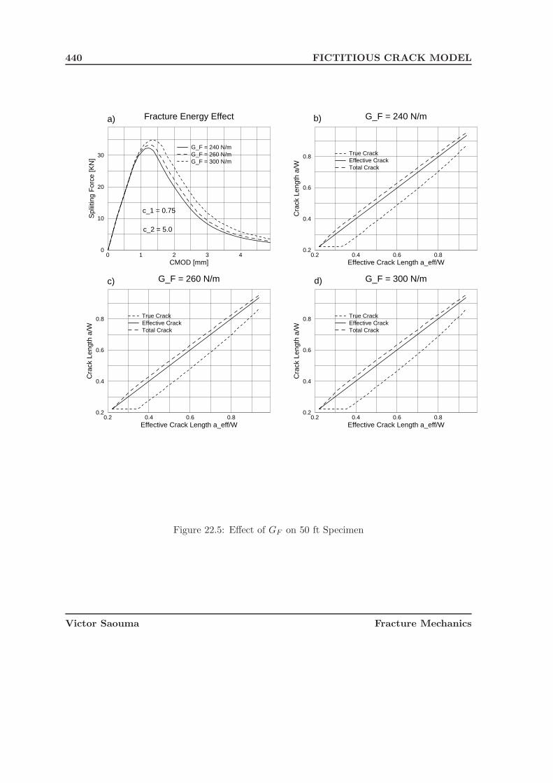
440 FICTITIOUS CRACK MODEL
0.2 0.4 0.6 0.8Effective Crack Length a_eff/W
0.2
0.4
0.6
0.8
Cra
ck L
engt
h a/
W
G_F = 260 N/m
True CrackEffective CrackTotal Crack
c_2 = 5.0
0 1 2 3 4CMOD [mm]
0
10
20
30
Spl
iitin
g F
orce
[KN
]
Fracture Energy Effect
G_F = 240 N/mG_F = 260 N/mG_F = 300 N/m
c_1 = 0.75
0.2 0.4 0.6 0.8Effective Crack Length a_eff/W
0.2
0.4
0.6
0.8
Cra
ck L
engt
h a/
W
G_F = 300 N/m
True CrackEffective CrackTotal Crack
a) b)
c) d)
0.2 0.4 0.6 0.8Effective Crack Length a_eff/W
0.2
0.4
0.6
0.8
Cra
ck L
engt
h a/
W
G_F = 240 N/m
True CrackEffective CrackTotal Crack
Figure 22.5: Effect of GF on 50 ft Specimen
Victor Saouma Fracture Mechanics

22.3 Validation 441
displacement beyond which no tensile stresses can be transmitted across the crack. Hencea series of analyses in which wc was varied from 0.54 to 1.6 mm, while w1 and GF werekept constant, were undertaken. The results of these analyses are shown in Figure 22.6.Interestingly we note that the peak load decreased with the increase in wc. These results
0.2 0.4 0.6 0.8Effective Crack Length a_eff/W
0.2
0.4
0.6
0.8
Cra
ck L
engt
h a/
W
w_c = 1.1 mm
True CrackEffective CrackTotal Crack
0 1 2 3 4CMOD [mm]
0
10
20
30
Spl
iitin
g F
orce
[KN
]
Crit. Crack Opening Effect
w_c = 0.54 mmw_c = 1.10 mmw_c = 1.60 mm
G_F = 240 N/mG_F = 240 N/m
0.2 0.4 0.6 0.8Effective Crack Length a_eff/W
0.2
0.4
0.6
0.8
Cra
ck L
engt
h a/
W
w_c = 1.6 mm
True CrackEffective CrackTotal Crack
a) b)
c) d)
0.2 0.4 0.6 0.8Effective Crack Length a_eff/W
0.2
0.4
0.6
0.8
Cra
ck L
engt
h a/
W
w_c = 0.54 mm
True CrackEffective CrackTotal Crack
Figure 22.6: Effect of wc on 50 ft Specimen
may be attributed to the substantial drop of s1 (fromf ′
t
4 ) required to maintain a constantGF or area under the softening curve. Furthermore, as wc increases, there is a slightincrease in both total crack and true crack. However, we note that for large wC values,the effective crack length becomes smaller than even the true crack. We currently haveno explanation for these results.
Victor Saouma Fracture Mechanics

442 FICTITIOUS CRACK MODEL
Effect of s1: Whereas in the original analysis s1 was taken asf ′
t
4 , the effect of its variation wasinvestigated through Figure 22.7, which indicates that this parameter has practically noeffect on the peak load, and a very limited one on the post-peak response. Similarly, itwas found that it also has limited effect on the crack length.
22.4 Conclusions
56 In summary, a new framework for linear/nonlinear fracture mechanics analysis of concretewas presented. Robustness of the algorithm was, to some extent, validated by the numeri-cal duplication of experimental results with standard material properties and no parametricoptimization.
57 This model is currently being extended to include the effect of a pressurized true crack andFPZ and to perform mixed mode analysis and 3D analyses. Future analyses will focus on itsapplication for the nonlinear analysis of cracked concrete dams.
22.5 Notation
m = Sub-domain index; either 1 or 2Ωm = Sub-domain mΩ = Domain of bodyb = Body force vectorbm = Body force vector for sub-domain mΓtm = Surface of sub-domain m subject to prescribed surface tractionsΓt = Surface of body subject to prescribed surface tractions
t = Prescribed surface traction vector
tm = Prescribed surface traction vector for sub-domain mu = Displacement vectorum = Displacement vector for sub-domain mδu = Virtual displacement vectorδum = Virtual displacement vector for sub-domain mL = Differential operator to obtain strain vector from displacement vectorε = Strain vectorεm = Strain vector for sub-domain mδε = Virtual strain vectorδεm = Virtual strain vector for sub-domain mD = Elastic stress strain matrixσ = Stress vectorσm = Stress vector for sub-domain mΓI = Interface surfaceΓIb
= Bonded interface surface
Victor Saouma Fracture Mechanics

22.5 Notation 443
0.2 0.4 0.6 0.8Effective Crack Length a_eff/W
0.2
0.4
0.6
0.8
Cra
ck L
engt
h a/
W
3 foot Specimen
s_1 = f’_t/5s_1 = f’_t/4s_1 = f’_t/3
0.0 0.2 0.4 0.6 0.8CMOD [mm]
0
20
40
60
80
Spl
iitin
g F
orce
[KN
]3 foot Specimen
s_1 = f’_t/5s_1 = f’_t/4s_1 = f’_t/3
0.0 0.2 0.4 0.6Crack Opening [mm]
0.0
0.5
1.0
1.5
2.0
2.5
Str
ess
[Mpa
]
Softening Bilinear Law
s_1 = f’_t/5s_1 = f’_t/4s_1 = f’_t/3
G_F = 240 N/m
G_F = 240 N/m
Total
Crack
Effective
Crack
True
Crack
a) b)
c)
Figure 22.7: Effect of s1 on 3 ft Specimen
Victor Saouma Fracture Mechanics

444 FICTITIOUS CRACK MODEL
ΓIc = Interface surface subject to cohesive stressestIm = Surface tractions on interface surfacetbm
= Surface tractions due to bonding on interface surface of sub-domain mtcm = Surface tractions due to cohesive stresses on interface surface of sub-domain mtb = Surface tractions due to bonding on interface surfacetc = Surface tractions due to cohesive stresses on interface surfaceλ = Lagrange multiplier vectorNum = Shape functions for displacements in sub-domain mum = Nodal displacement vector for sub-domain mNλ = Shape functions for Lagrange multipliers on bonded interface
λ = Nodal Lagrange multiplier vector; total nodal Lagrange multiplier vector atbeginning of increment
Bm = Strain-displacement matrix for sub-domain mKm = Stiffness matrix for sub-domain mfm = Applied load vector for sub-domain mQm = Operator matrix for load vector due to Lagrange multipliers on bonded interface
surface of sub-domain mfcm = Load vector due to cohesive stresses on interface surface of sub-domain mI = Identity matrixα = Penalty numberf = Arbitrary applied load vectori = Increment number, element number, or node numberβi = Total load factor at beginning of increment iΔβi = Incremental load factor for increment in = Iteration numberΔun = Incremental nodal displacement vector at beginning of iteration nδun = Correction to incremental nodal displacement vector for iteration nΔun+1 = Incremental nodal displacement vector at end of iteration nΔβn = Incremental load factor at beginning of iteration nδβn = Correction to incremental load factor for iteration nΔβn+1 = Incremental load factor at end of iteration nu = Nodal displacement vector at beginning of incrementKα = Penalized stiffness matrixβ = Load factor at beginning of iteraction nfnc = Load vector due to cohesive stresses on interface at beginning of iteration npn = Reaction vector at beginning of iteration nrn = Residual load vector at beginning of iteration nδuT = Nodal tangent displacement vector for incrementδun
r = Correction to incremental nodal displacement vector due to residual loadsfor iteration n
Δλn
= Incremental nodal Lagrange multiplier vector at beginning of iteration n
δλnr = Correction to incremental nodal Lagrange multiplier vector due to residual
Victor Saouma Fracture Mechanics
22.5 Notation 445
loads for iteration n
δλT = Nodal Lagrange multiplier vector due to tangent displacement for increment
Δλn+1
= Incremental nodal Lagrange multiplier vector at end of iteration nn = Normal vectorft = Uniaxial tensile strength
Victor Saouma Fracture Mechanics

446 FICTITIOUS CRACK MODEL
Victor Saouma Fracture Mechanics
Chapter 23
INTERFACE CRACK MODEL
This chapter was chapter 6 of the PhD thesis of Cervenka
1 This chapter discusses the nonlinear modeling of concrete using a discrete crack fracture me-chanics based model. It addresses two important issues: mixed mode fracture in homogeneousmaterials and interface fracture. A new three-dimensional interface crack model is derived. Themodel is a generalization of classical Hillerborg’s fictitious crack model, which can be recoveredif shear displacements are set to zero. Several examples are used to validate the applicabilityof the proposed interface crack model. First, direct shear tests on mortar joints are used totest the model performance in the shear-compression regime. The more complicated combina-tion of shear-tension is investigated using large biaxial tests of concrete-rock interfaces. Theapplicability to mixed mode cracking in homogeneous concrete is tested using experiments onmodified Iosipescu’s shear beam and anchor bolt pull-out tests.
23.1 Introduction
2 The assumption of singular stresses at the crack tip is mathematically correct only within theframework of linear elastic fracture mechanics, but physically unrealistic.
3 In concrete materials, a fracture process zone (Section ??) exists ahead of the crack tip.The most popular model simulating this behavior is Hillerborg’s fictitious crack model (FCM)described in Section ?? and Figure ??. In a previous work, the classical FCM model wasimplemented by (Reich 1993) for mode I crack propagation, and extended to account for theinfluence of water pressure inside the crack.
4 The classical FCM model, Chapter 22, defines a relationship between normal crack openingand normal cohesive stresses, and assumes that there are no sliding displacements nor shearstresses along the process zone. This assumption is only partially valid for concrete materials.Based on experimental observations, it is indeed correct that a crack is usually initiated in puremode I (i.e. opening mode) in concrete, even for mixed mode loading. However, during crackpropagation, the crack may curve due to stress redistribution or non-proportional loading, and

448 INTERFACE CRACK MODEL
significant sliding displacements develop along the crack as schematically shown in Figure 23.1.Therefore, it is desirable to incorporate these shear effects into the proposed crack model.
τσ
u
t
Figure 23.1: Mixed mode crack propagation.
5 Finally for concrete dams, it is well accepted that the weakest part of the structure is thedam-foundation interface, which is also the location of highest tensile stresses and lowest tensilestrength. Given the scope of this work, as described in Chapter ??, it is necessary to addressthis problem.
6 Hence, the two major objectives of this chapter are:(1) Modification of the FCM model to account for shear effects along both the fracture
process zone and the true crack.(2) Development of an interface model based on fracture mechanics to simulate cracking
along rock-concrete interfaces.
7 The FCM model, within the framework of a discrete crack implementation, can be visualizedas an interface between two identical materials. Therefore, we can develop a general modelwhich addresses both objectives.
8 Interface elements were first proposed by (Goodman, R.E., Taylor, R.C. and Brekke, T.C.,1968) to model non-linear behavior of rock joints. Since then, numerous interface constitutivemodels have been proposed for a wide range of applications such as rock-joints (Goodman, R.E.,Taylor, R.C. and Brekke, T.C., 1968) masonry structures (Lotfi 1992) and concrete fracture(Stankowski 1990) (Feenstra P.H. and J. 1991) and (Carol, I., Bazant, Z.P. and Prat, P.C., 1992).
9 In the following section an interface crack model will first be proposed, and then it will beused to simulate cracking both in homogeneous concrete and along a rock-concrete interface.The presented model is a modification of the one first proposed by (Carol, I., Bazant, Z.P. and
Victor Saouma Fracture Mechanics

23.2 Interface Crack Model 449
0.0 0.5 1.0 1.5 2.0CMOD [mm]
0.0
0.5
1.0
1.5
2.0
2.5
Ver
tical
Loa
d [k
N]
12
3
1. Solid Concrete GF = 158.9 N/m
2. Solid Limestone GF = 41.8 N/m
3. Limestone-Concrete GF = 39.7 N/m
Figure 23.2: Wedge splitting tests for different materials, (Saouma V.E., and Cervenka, J. andSlowik, V. and Chandra, J.M. 1994)
Prat, P.C., 1992).
23.2 Interface Crack Model
10 The objective is to develop a physically sound model, yet simple enough so that all its para-meters can be easily derived from laboratory tests. The model should be capable of simulatingthe behavior of rock-concrete and concrete-concrete interfaces.
11 Experimental data (Saouma V.E., and Cervenka, J. and Slowik, V. and Chandra, J.M. 1994)on rock-concrete interfaces show (Figure 23.2) that the decrease in tensile strength is not abrupt,but is rather gradual. This is caused by the presence of the fracture process zone, along whichthe energy of the system is gradually dissipated.
12 In the present model, the rock-concrete contact is idealized as an interface between twodissimilar materials with zero thickness. Thus, the objective is to define relationships betweennormal and tangential stresses with opening and sliding displacements. The notation used inthe interface model is illustrated in Figure 23.2.
13 The major premises upon which the model is developed are:(1) Shear strength depends on the normal stress.(2) Softening is present both in shear and tension.(3) There is a residual shear strength due to the friction along the interface, which depends
on the compressive normal stress.
Victor Saouma Fracture Mechanics

450 INTERFACE CRACK MODEL
Material 1
Material 2 Material 2
Material 1
,,
Interface Interface Model
u σu τx
y
u ,
u ,u ,
τ
τσ
x
y
z
1
2
Figure 23.3: Interface idealization and notations.
Victor Saouma Fracture Mechanics

23.2 Interface Crack Model 451
(4) Reduction in strength, i.e. softening, is caused by crack formation.(5) There is a zero normal and shear stiffness when the interface is totally destroyed.(6) Under compressive normal stresses neither the shear and nor the normal stiffnesses
decrease to zero. In addition, should a compressive stress be introduced in the normal directionfollowing a full crack opening, two faces of the interface come to contact, and both tangentialand normal stiffnesses become nonzero.
(7) Irreversible relative displacements are caused by broken segments of the interface mate-rial and by friction between the two crack surfaces.
(8) Roughness of the interface causes opening displacements (i.e. dilatancy) when subjectedto sliding displacements.
(9) The dilatancy vanishes with increasing sliding or opening displacements.
14 Figure 23.4 illustrates the probable character of the fracturing process along an interface.
Fracture Process Zone InterfaceTrue Crack
τ
σ
Intact
Figure 23.4: Interface fracture.
15 In the proposed model the strength of an interface is described by a hyperbolic failurefunction:
F = (τ21 + τ2
2 ) − 2 c tan(φf )(σt − σ) − tan2(φf )(σ2 − σ2t ) = 0 (23.1)
where:
• c is the cohesion.
• φf is the angle of friction.
• σt is the tensile strength of the interface.
• τ1 and τ2 are the two tangential components of the interface traction vector.
• σ is the normal traction component.
Victor Saouma Fracture Mechanics

452 INTERFACE CRACK MODEL
16 The shape of the failure function in two-dimensional case is shown in Figure 23.5, and itcorresponds to the failure criteria first proposed by (Carol, I., Bazant, Z.P. and Prat, P.C., 1992).The general three-dimensional failure function is obtained by mere rotation around the σ-axis.
φ
tan( )φf
Final FailureFunction
Initial FailureFunction
σ
τ
c
σ
tan( )f
t
1
1
Figure 23.5: Failure function.
17 The evolution of the failure function is based on a softening parameter uieff which is thenorm of the inelastic displacement vector u
i. The inelastic displacement vector is obtained bydecomposition of the displacement vector u into an elastic part u
e and an inelastic part ui. The
inelastic part can subsequently be decomposed into plastic (i.e. irreversible) displacements up
and fracturing displacements uf . The plastic displacements are assumed to be caused by friction
between crack surfaces and the fracturing displacements by the formation of microcracks.
F = F (c, σt, φf ), c = c(uieff), σt = σt(uieff)
u = ue + u
i, ui = u
p + uf
uieff = ||ui|| = (uix2+ ui
y2+ ui
z2)1/2
(23.2)
Victor Saouma Fracture Mechanics

23.2 Interface Crack Model 453
18 In this work both linear and bilinear relationship are used for c(uieff) and σt(uieff).
c(uieff) = c0(1 − uieff
wc) ∀ uieff < wc
c(uieff) = 0 ∀ uieff ≥ wc
wc =2GIIa
F
c0
⎫⎪⎪⎬⎪⎪⎭ linear for cohesion
c(uieff) = c0 + uieff s1c−c0w1c
∀ uieff < w1c
c(uieff) = sc(1 − uieff−w1c
wc−w1c) ∀ uieff ∈ 〈w1c, wc〉
c(uieff) = 0 ∀ uieff > wc
wc =2GIIa
F−(s1c+c0)w1c
s1c
⎫⎪⎪⎪⎪⎬⎪⎪⎪⎪⎭
bi-linear for cohesion
(23.3)
σt(uieff) = σt0(1 − uieff
wσ) ∀ uieff < wσ
σt(uieff) = 0 ∀ uieff ≥ wσt
wσ =2GI
F
σt0
⎫⎪⎪⎬⎪⎪⎭ linear for tensile strength
σt(uieff) = σt0 + uieff s1σ−σt0
w1σ∀ uieff < w1σ
σt(uieff) = s1σ(1 − uieff−w1σ
wσt−w1σ) ∀ uieff ∈ 〈w1σ , wσ〉
σt(uieff) = 0 ∀ uieff > wσ
wσ =2GI
F−(s1σ+σt0)w1σ
s1σ
⎫⎪⎪⎪⎪⎬⎪⎪⎪⎪⎭
bi-linear fortensile strength
(23.4)
where GIF and GIIa
F are mode I and II fracture energies. s1c, w1c and s1σ, w1σ are the coordinatesof the breakpoint in the bi-linear softening laws for cohesion and tensile strength respectively.
19 The critical opening and sliding corresponding to zero cohesion and tensile strength aredenoted by wσ and wc respectively, and they are determined from the condition that the areaunder the linear or bilinear softening law must be equal to GI
F and GIIaF respectively. The
significance of these symbols can be best explained through Figure 23.6.
GF
IG
IIaF
c
ww
s
σtσt 0 c0
s1c
1cwσ
1σ
1σuieff wc
uieff
Figure 23.6: Bi-linear softening laws.
Victor Saouma Fracture Mechanics

454 INTERFACE CRACK MODEL
20 It should be noted that GIIaF is not the pure mode II fracture energy (i.e. the area under a
τ -ux curve), but rather is the energy dissipated during a shear test with high confining normalstress. This parameter was first introduced by (Carol, I., Bazant, Z.P. and Prat, P.C., 1992)in their microplane model. This representation seems to be more favorable to the pure modeII fracture energy GII
F . The determination of GIIF would require a pure shear test without
confinement, which is extremely difficult to perform. Alternatively, a GIIaF test requires a large
normal confinement, and is therefore easier to accomplish. Furthermore, if GIIF is used, the
whole shear-compression region of the interface model would be an extrapolation from theobserved behavior, whereas the second approach represents an interpolation between the upperbound GIIa
F and the lower bound GIF .
21 The residual shear strength is obtained from the failure function by setting both c and σt
equal to 0, which corresponds to the final shape of the failure function in Figure 23.5 and isgiven by:
τ21 + τ2
2 = tan2(φf ) σ2 (23.5)
22 Stiffness degradation is modeled through a damage parameter, D ∈ 〈0, 1〉, which is a relativemeasure of the fractured surface. Thus, D is related to the secant of the normal stiffness Kns
in the uniaxial case:
D =Af
Ao= 1 − Kns
Kno(23.6)
where Kno is the initial normal stiffness of the interface; Ao and Af are the total interface areaand the fractured area respectively.
23 It is assumed, that the damage parameter D can be determined by converting the mixedmode problem into an equivalent uniaxial one (Figure 23.7). In the equivalent uniaxial problemthe normal inelastic displacement is set equal to uieff. Then, the secant normal stiffness can bedetermined from:
Kns =σ
u − up=
σt(uieff)
ue + up + uf − up=
σt(uieff)
σt(uieff)/Kno + (1 − γ)uieff(23.7)
where γ is the ratio of irreversible inelastic normal displacement to the total value of inelasticdisplacement.
24 Experimentally, γ can be determined from a pure mode I test through:
γ =up
ui(23.8)
where up is the residual displacement after unloading and ui is the inelastic displacement beforeunloading. (Figure 23.7).
25 For concrete, γ is usually assumed equal to 0.2 (Dahlblom and Ottosen 1990) or 0.3 (Alvaredoand Wittman 1992). Then, the evolution of the damage parameter D is defined by formula:
D = 1 − σt(uieff)
σt(uieff) + (1 − γ)uieffKno(23.9)
Victor Saouma Fracture Mechanics

23.2 Interface Crack Model 455
σ
u
noK
K ns
σ i
σ
u = uγ u
u = ui ieff
ip i
GFI
Figure 23.7: Stiffness degradation in the equivalent uniaxial case.
which is obtained by substituting Equation 23.7 into Eq. 23.6.
26 The stress-displacement relationship of the interface is expressed as:
σ = αE(u − up) (23.10)
where: (a) σ is the vector of tangential and normal stress at the interface.
σ = {τ1, τ2, σ}T (23.11)
(b) α is the integrity parameter defining the relative active area of the interface, and it isrelated to the damage parameter D.
α = 1 − |σ| + σ
2|σ| D (23.12)
It should be noted that α can be different from 1 only if the normal stress σ is positive (i.e.the interface is in tension). In other words, the damage parameter D is activated only if theinterface is in tension. In compression, the crack is assumed to be closed, and there is fullcontact between the two crack surface. The activation of D is controlled through the fraction|σ|+σ2|σ| , which is equal to one if σ is positive, and is zero otherwise.
(c) E is the elastic stiffness matrix of the interface.
E =
⎡⎢⎣ Kto 0 0
0 Kto 00 0 Kno
⎤⎥⎦ (23.13)
27 It should be noted, that the off-diagonal terms in the elastic stiffness matrix E of the interfaceare all equal to zero, which implies that no dilatancy is considered in the elastic range. Thedilatancy is introduced later after the failure limit has been reached through the iterative
Victor Saouma Fracture Mechanics

456 INTERFACE CRACK MODEL
solution process. The dilatancy of the interface is given by dilatancy angle φd, which is againassumed to be a function of uieff. In the proposed model, a linear relationship is assumed:
φd(uieff) = φd0(1 − uieff
udil) ∀uieff ≤ udil
φd(uieff) = 0 ∀uieff > udil
(23.14)
where udil is the critical relative displacement after which, the interface does not exhibit thedilatancy effect any more, and φd0 is the initial value of the dilatancy angle.
23.2.1 Relation to fictitious crack model.
28 It is possible to prove that the proposed interface crack model (ICM) reduces to Hillerborg’sfictitious crack model in the case of zero sliding displacements.
[FCM a special case of ICM.] We assume that all shear displacements are zero. Then, theinterface stresses develop only along the σ-axis in the σ× τ1 × τ2 space (Figure 23.5). After thetensile strength σt is reached, softening starts, and the stress in the interface is given by:
σ = σ(uiz) (23.15)
Normal traction σ is now a function of the normal inelastic displacement uiz only, since for zero
sliding displacements, uieff is equivalent to uiz. The total opening uz of the interface is given by:
uz =σ(ui
z)
Kno+ ui
z
If the limiting case of Kno equal to infinity is considered, then uiz becomes equivalent to uz,
and the normal stress in Equation 23.15 becomes a function of the interface opening only:
limKno→∞
σ = σ(uiz) = σ(uz) = σ(COD) (23.16)
which is precisely the definition of Hillerborg’s fictitious crack model.
23.3 Finite Element Implementation
29 The finite element implementation of the interface crack model previously presented will bediscussed in this section. The implementation of a nonlinear model into a finite element codeconsists of three major subtasks:
1. Interface element formulation.
2. Constitutive driver for the computation of internal forces.
3. Non-linear solution algorithm on the structural level.
Victor Saouma Fracture Mechanics

23.3 Finite Element Implementation 457
23.3.1 Interface element formulation.
30 Standard interface elements are used in this work. The element stiffness matrix is computedusing the well known relation:
Ke =
∫Ae
BTEB dA (23.17)
where E is the interface material stiffness matrix, given by Equation 23.13, and B is the matrixrelating element nodal displacements ue to slidings and openings along the interface:
u =
1/2Nen∑i
Ni(u+i − u−
i ) = Bue (23.18)
where u+i and u
−i denote the element nodal displacements in the local coordinate system of the
interface on the upper and lower interface surface respectively. Given this definition, matrix B
is equal to:
B =[−B1T , · · · , −Bp+1T , +B1T , · · · , +Bp+1T
](23.19)
where submatrix Bi is a diagonal matrix of shape functions Ni(ζ, η) corresponding to node i.In three-dimensional case it has the form:
Bi =
⎡⎢⎣ Ni(ζ, η) 0 0
0 Ni(ζ, η) 00 0 Ni(ζ, η)
⎤⎥⎦ (23.20)
and in two-dimensional case it is given by:
Bi =
[Ni(ζ) 0
0 Ni(ζ)
](23.21)
Subscript i is a node numbering index on one element surface ranging from 1 to Nen
2 , whereNen is the total number of element nodes, p is the order of the interface element, and is equalto (Nen
2 − 1). Finally, ζ and η are the natural coordinates of the interface element.
31 This definition of matrix B corresponds to the element numbering shown in Figure 23.8 forseveral two- and three-dimensional interface elements.
32 The transformation from global to local coordinate system of the interface element is accom-plished through the transformation matrix T , which in general three-dimensional case is:
T =
⎡⎢⎣ v
T1
vT2
vT3
⎤⎥⎦ (23.22)
The rows of the transformation matrix T are formed by vectors vi defined by following formulas:
v1 =
∂x∂ζ
||∂x∂ζ ||, v3 =
∂x∂ζ × ∂x
∂η
||∂x∂ζ × ∂x∂η ||
v2 = v3 × v1, (23.23)
Victor Saouma Fracture Mechanics

458 INTERFACE CRACK MODEL
1 2
3 4
1
4
12
4
5
6
1
7
1
2
3
57
8
9
16
1
84
6
12
6
23
56
3
2
3
4
5
8
9
11
10
2
3
4
76
510
11
12
13
1415
Figure 23.8: Interface element numbering.
Victor Saouma Fracture Mechanics

23.3 Finite Element Implementation 459
33 The two-dimensional case can be recovered from the two preceding formulas by deleting thelast row in matrix T and considering the following definition of vectors vi.
v1 =
∂x∂ζ
||∂x∂ζ ||, v2 = {−v1y, v1x} (23.24)
Local coordinate systems defined by these transformations are shown in Figure 23.9.
y’
x’
y’z’
x’
ζ
η
ζ
Figure 23.9: Local coordinate system of the interface element.
23.3.2 Constitutive driver.
34 The mathematical theory of plasticity is used in the development of the constitutive driverfor the interface crack model. On the constitutive level in the sense of finite element implemen-tation, the problem can be stated as follows:
35 For a given stress state σn, softening parameter uieffn and displacement increment Δun,
determine a new stress state σn+1 and corresponding value of softening parameter uieffn+1. In
both states n and n + 1, the failure criterion must be satisfied:
Fn(σn, uieffn ) = 0 ∧ Fn+1(σn+1, u
ieffn+1) = 0 (23.25)
These two conditions are equivalent to an incremental form of the consistency condition (Equa-tion ??):
ΔF = Fn+1 − Fn = 0 (23.26)
36 Because the failure function is assumed to be satisfied for state n, it is necessary to alsoensure the satisfaction of the failure function at state n + 1.
37 In this work, plasticity theory is used to describe the evolution of the failure function based onthe softening parameter uieff, which is the euclidean norm of the inelastic displacement vector.
Victor Saouma Fracture Mechanics

460 INTERFACE CRACK MODEL
The inelastic displacements are subsequently decomposed according to Equation 23.8. Thus,plastic and fracturing effects can be separated.
38 The elastic predictor is given by:
σe = σn + EΔun (23.27)
where σe are the trial tractions outside the failure surface if a totally elastic behavior is con-sidered. The inelastic corrector returns the trial stress state back to the failure surface:
σn+1 = σe − ΔλE m (23.28)
where Δλ is the inelastic multiplier and m is the direction of the inelastic displacements.Inelastic multiplier Δλ is determined from the failure condition at state n + 1.
Fn+1(σe − ΔλE m, uieffn+1) = 0 (23.29)
39 In the three dimensional space σ × τ1 × τ2, the geometrical interpretation of this conditionis the determination of an intersection of a line emanating from point σe in the direction Em
with the moving failure surface (Figure 23.10).
40 The failure surface, F = 0, expands or shrinks depending on the softening introduced throughuieff. This is schematically shown in Figure 23.10 for a two-dimensional case.
tan( )φdKnKt
c
σ
σ
0
σ
F = 0
F = 0
Q = 0
0
0
1
1
1
τ
σ
c1
Q = 00
σ1 0ttσ
e
0
l = E m
1
li i
l1
Figure 23.10: Algorithm for interface constitutive model.
41 The increment of the plastic multiplier Δλ is computed by solving a quadratic equationobtained by considering the particular form of the failure function 23.1 in Equation 23.29.
Victor Saouma Fracture Mechanics

23.3 Finite Element Implementation 461
42 For this case, the failure function is equal to:
F = (τ21 n+1 + τ2
2 n+1) − 2 c tan(φf )(σt − σn+1) − tan2(φf )(σ2n+1 − σ2
t ) = 0 (23.30)
43 To this equation, we substitute the expression for the new stress state σn+1, which are equalto (Equation 23.28):
τ1n+1 = τ1e − ΔλKtom1 = τ1e − Δλl1τ2n+1 = τ2e − ΔλKtom2 = τ2e − Δλl2σn+1 = σe − ΔλKnom3 = σe − Δλl3
(23.31)
44 The result of this substitution is a quadratic equation with roots:
Δλ1,2 =−B ±
√B2 − 4AC
2A(23.32)
whereA = l21 + l22 − μ2l23B = 2μ2σel3 − 2l1τ1e − 2l2τ2e − 2cμl3C = τ2
1 e + τ22 e − 2cμσt + μ2σ2
e + μ2σt
45 The required solution must satisfy the following conditions.
Δλ > 0 ∧ Δλ = min(Δλ1,Δλ2) (23.33)
46 In the previous equations, l1, l2 and l3 are components of vector l indicating the direc-tion of inelastic return in the stress space, and they are related to the direction of inelasticdisplacements m through the stiffness matrix E.
l = Em (23.34)
47 The direction of inelastic displacements m is defined as the normal vector to the plasticpotential Q (Figure 23.10), which is defined using the dilatancy angle φd(u
ieff) as:
Q = τ21 + τ2
1 − (Kn
Kttan φd)
2σ2 = 0 (23.35)
48 For the definition of m, we must distinguish between the case, when the return directionm can be determined on the basis of Q, and the pathological case of the apex of Q, when thenormal m cannot be constructed. For this case, m is defined by connecting the trial tractionsσe with the origin of the σ × τ1 × τ2 space (Figure 23.11):
m =
⎧⎪⎨⎪⎩
τ1/Kto
τ2/Kto
σ/Kno
⎫⎪⎬⎪⎭ if ||τ ||
σ ≤ 1tan φd
Kto
Kno∧ σ > 0
m =
⎧⎪⎨⎪⎩
τ1
τ2√τ21 + τ2
2 tan φd
⎫⎪⎬⎪⎭ otherwise
(23.36)
Victor Saouma Fracture Mechanics

462 INTERFACE CRACK MODEL
tan( )φdKnKt
c
F = 0τ
σ
1
σt
Case (2)
Case (1)σ
σe
e
Q = 0
l = E m
l = E m
Figure 23.11: Definition of inelastic return direction.
49 At this stage, we can identify three major steps to the proposed algorithm:
1. Elastic predictor:σe = σn + EΔun (23.37)
2. Inelastic corrector simultaneously satisfying the following two equations:
Fn+1(σe − ΔλEm, uieffn+1) = 0
uieffn+1 = uieff
n + ||Δλm|| (23.38)
3. Fracturing corrector:Es = αE
up = u − E
−1s σn+1
(23.39)
50 In the fracturing corrector, the inelastic displacements due to friction and microcracks de-velopment are separated. This separation is controlled by the damage parameter D defined byEquation 23.9. The evolution of damage parameter D is defined by converting the mixed modeproblem into an equivalent uniaxial case as described in Section 23.2.
51 The complete algorithm of the interface constitutive driver is described in Algorithm 23.3.2and is shown schematically on Figure 23.10.
Victor Saouma Fracture Mechanics

23.3 Finite Element Implementation 463
[ICM constitutive driver.]
• Input: σn, uieffn and Δun
• σn+1 = σn + αE Δun
• if F (σn+1, uieffn ) > 0
– Update σn, and Δun such that F (σn, uieffn ) = 0.
– Elastic predictor: σn+1 = σn + E Δun
– Inelastic corrector:
∗ uieffn+1 = uieff
n
∗ Do
· Evaluate return direction m
· Determine dλ such that F (σn+1 − dλEm, uieffn+1) = 0
· uieffn+1 = uieff
n+1 + ||dλm||· σn+1 = σn+1 − dλEm
∗ While dλ < ε
– Fracturing corrector:
α = 1 − |σ|+σ2|σ| D(uieff
n+1)
Es = αE
up = u − E
−1s σn+1
• Output: σn+1, uieffn+1
52 Figure 23.12 illustrates a simple example of direct tension test with the proposed interfacecrack model. It demonstrates the accuracy of the proposed algorithm as the normal stressesare always correctly evaluated for the given displacements, and there is no loss of accuracywhen larger increment steps are used. This is a direct consequence of the geometrical approachduring the inelastic corrector phase of the algorithm and the displacement based softening. Thisexample also illustrates the ability of the proposed model to simulate Hillerborg’s fictitious crackmodel.
53 The robustness of the interface constitutive driver can also be tested by analyzing an exampleof shear under fixed tension in the normal direction. This is clearly an unstable problem onthe structural level, since following certain sliding displacement the tensile strength is lowerthan the originally applied normal stress, and the specimen fails in an unstable manner. Thisimplies that on the structural level the solution cannot converge. However, the algorithm shouldnot fail on the constitutive level, which could occur in some plasticity based models in which
Victor Saouma Fracture Mechanics

464 INTERFACE CRACK MODEL
0.00 0.02 0.04 0.06 0.08Displacement uy [in]
0.0
20.0
40.0
60.0
80.0
100.0
120.0
Nor
mal
Str
ess
σ [p
si]
22 increments 11 increments 3 increments
Figure 23.12: Influence of increment size.
the consistency condition is used to determine the increment of the plastic multiplier dλ. Inthese formulations, due to the snap-back on the constitutive level, a negative value of dλ isobtained, and the second Kuhn-Tucker condition (Equation ??) is not satisfied causing themodel to fail on the constitutive level. This is clearly an undesirable feature since a snap-backon the constitutive level could occur even in otherwise stable problems. To investigate thebehavior of the proposed interface model in the shear-tension regime, a simple example of twoquadrilateral elements connected by an interface element is analyzed. In the first incrementtensile tractions are applied on the upper element, and in the subsequent increments horizontaldisplacements are prescribed for the upper element. The resulting load-displacement curve isshown in Figure 23.13.
0.000 0.005 0.010 0.015 0.020 0.025 0.030CSD [mm]
0.0
0.5
1.0
1.5
2.0
Shea
r st
ress
τ [
MPa
]
σ=const.u
Figure 23.13: Shear-tension example.
54 We observe the tendency for snap-back behavior when CSD ≈ 0.0245 mm. After this point,due to the unstable nature of the problem, convergence on the structural level could no longer
Victor Saouma Fracture Mechanics

23.3 Finite Element Implementation 465
be achieved, however no problems on the constitutive level are observed.
23.3.3 Non-linear solver.
55 The proposed interface crack model is clearly a nonlinear material formulation, and therefore,a finite analysis including this material formulation involves a system of nonlinear equations.Such system can be solved, for instance, by the Newton-Raphson method. To exploit thefull Newton-Raphson method a tangent stiffness matrix would have to be computed at eachiteration. The incremental tangent stiffness matrix for the proposed material formulation canbe computed from the incremental stress-displacement relationship:
Δσn = E Δun − ΔλEm (23.40)
when multiply the last term by a fraction which is equal to unity:
Δσn = E Δun − ΔλEmn
TEΔun
nT EΔun(23.41)
where n is the normal vector to the failure surface passing through the trial stress state σe
(Equation 23.27).
56 From this equation it is possible to derive a formula for an incremental tangent materialstiffness matrix ET :
Δσn = ET Δun (23.42)
where:
ET = E
(I − Δλ
EmnTE
nT EΔun
)(23.43)
57 In this particular case, the new stress state is computed using the iterative process describedin Algorithm 23.3.2. Therefore, the incremental stress-displacement is given by a sum:
Δσn = E Δun −Niter∑i=1
(ΔλiEmi) (23.44)
where Niter is the number of iterations in the inelastic corrector part of Algorithm 23.3.2.Following similar arguments leading to equation 23.43, the incremental tangent stiffness iscomputed by the following expression:
ET = E
⎡⎣I −
Niter∑i=1
(Δλi
EminTi E
nTi EΔun
)⎤⎦ (23.45)
58 During softening, the tangent matrix ET becomes negative. In addition, the matrix becomesalso unsymmetric due to the dilatancy, which is introduced in the softening regime of the
Victor Saouma Fracture Mechanics

466 INTERFACE CRACK MODEL
interface model. This would imply the need to store the full stiffness matrix on the structurallevel, and a method for solving unsymmetric and non-positive system of equations would haveto be adopted. This is clearly not an efficient approach, since only few elements will be affectedby the non-linear behavior (i.e. interface elements), and therefore, only small portions of thestructural stiffness matrix will be unsymmetric.
59 On the other hand, it can be expected that the initial stiffnesses of the interface elementsare very large, and in some cases, they represent penalty numbers modeling a rigid contact.This means that it is not possible to use the initial structural stiffness throughout the wholeiterative process, as it would result in an excessive number of iterations.
60 In this work two approaches are suggested to mitigate this problem:(1) Use of secant-Newton method to accelerate the convergence on the structural level.(2) Use of secant interface stiffness on the element level while preserving its positiveness
and symmetry.Both methods are supplemented with the line-search technique of (Crisfield, M.A. 1991).
23.3.4 Secant-Newton method.
61 The secant-Newton method is described in detail in (Crisfield, M.A. 1991). In this method,it is not necessary to recompute the structural stiffness matrix at each iteration, but rather thevector of iterative displacement corrections is updated to satisfy the secant relationship.
du∗i
ri=
du∗i−1
ri − ri−1(23.46)
62 For one-dimensional case, the meaning of this formula is illustrated by Figure 23.14.
du
rr
du
K
Ks
or - r
F
u(i-1)
(i-1)
(i-1) (i)
(i)
(i)**
Figure 23.14: Secant relationship.
63 In this work, (Davidon, W.C. 1968) rank-one quasi-Newton update is used, and the corrected
Victor Saouma Fracture Mechanics

23.3 Finite Element Implementation 467
iterative update of the displacement vector in iteration i is equal to:
du∗i = Adui + Bdu
∗i−1 + Cdui−1 (23.47)
where dui is the iterative update of the displacement vector computed in iteration i by solving:
dui = K−1
ri (23.48)
where K is the structural stiffness matrix, and ri are residual forces at iteration i. The staredsymbols, u
∗i and u
∗i−1, represent the displacement vector updates based on the secant-Newton
corrections (Equation 23.47), and coefficients A, B and C are given by (Davidon, W.C. 1968):
C =(du∗
i−1+dui−dui−1)T ri
(du∗
i−1+dui−dui−1)T (ri−ri−1)
A = 1 − C, B = −C(23.49)
23.3.5 Element secant stiffness.
64 It is also possible to employ the secant formula (Eq. 23.46) on the element level. Consideringthe diagonal form of the material stiffness matrix E, it is possible to determine its secant formfrom the stress and displacement corrections in each iteration.
Kit1 =
τ i1n+1
−τ i−11 n+1
Δuixn+1−Δui−1
x n+1
Kit2 =
τ i2n+1
−τ i−12 n+1
Δuiyn+1
−Δui−1y n+1
Kin =
σin+1−σi−1
n+1
Δuizn+1−Δui−1
z n+1
(23.50)
65 To preserve the positiveness of the material stiffness matrix a minimal value for shear andnormal stiffnesses must be specified. In this work the shear and normal stiffnesses cannot beless than 10−8 times their original value. This number is based on the assumption that theratio of the lowest elastic modulus to the largest interface stiffness is below 10−4. This ratioshould be sufficient in most practical problems, since the interface stiffness can be estimatedfrom:
Kn =E
t(23.51)
where t is the interface thickness. Thus, the ratio EKinterface ≈ 10−4 corresponds to the assump-
tion of interface thickness being equal to 10−4 times a unit length of the problem. This shouldbe adequate for the types of of problems under consideration in this work. Alternatively, weconsider an extreme case of Kinterface of the same order as E (i.e. t ≈ problem unit). Thenafter cracking, the interface stiffness will be is reduced to 10−8 times its original value, and itis possible to estimate the condition number of the system using the elastic modulus, maximaland minimal element sizes.
κ ≈ Kelemmax
Kinterfacemin
≈ Ehmax
(Eh2min)/t × 10−8
≈ 1014 (23.52)
Victor Saouma Fracture Mechanics

468 INTERFACE CRACK MODEL
In the formula, the element sizes were assumed to be in the range of the order 〈10−2, 102〉.66 The loss of accuracy due to finite precision arithmetic is given by:
s = p − log(κ) (23.53)
where p is the number of significant digits in the computer representation of real numbers ands is the accuracy of the solution. The system will become ill-conditioned when:
s ≤ 0 (23.54)
67 A real number f is internally represented in a computer memory by three integers m, β ande.
f = .m × βe (23.55)
The mantissa m gives the number of significant digits. For double precision data type, m isusually stored in 52 bits, which corresponds to approximately 16 significant digits. Therefore,the accuracy after decomposition is in the worst possible scenario equal to 2 (Equation 23.53),which is of course an unacceptable level of accuracy. However, it should be kept in mind thatthis is a worst case scenario, and it would be unrealistic to have a ratio of largest to smallestelement of the order of 104, as was assumed in Equation 23.52.
23.3.6 Line search method.
68 Numerical experiments showed, that often the diagonal approximation of the secant stiffnessunderestimates the true stiffness of the interface and allows for excessive interface sliding. Theexcessive sliding in turn introduces large dilatancy effects and high compressive stresses in thenormal direction in the subsequent iteration. These high compressive stresses and the frictionalproperties of the interface combined with the excessive slidings will cause large shear stresses,which may not be in equilibrium with the rest of the finite element mesh. Due to this, theresulting high residual forces attempt to slide the interface backwards, but since the stiffnessof the interface is underestimated, the backward sliding is too large, and the iteration processdiverges. This problem can be solved by combining the previously discussed secant-methodswith line searches.
69 The fundamental principle behind the line search method (Crisfield, M.A. 1991) is to de-termine a scaling factor ω, for the current iterative displacement correction, such that thefunctional of total potential energy is stationary.
Π(ω) = Π(ui−1 + ωdui) = Π(ω) +∂Π(ω)
∂u(ω)
∂u(ω)
∂ωδω (23.56)
The functional Π(ω) would be stationary if the last term is equal to zero. It can be shown,(Crisfield, M.A. 1991), that the partial derivative of total potential energy Π(ω) with respect
Victor Saouma Fracture Mechanics

23.3 Finite Element Implementation 469
to displacements u(ω) is equal to the vector of residual forces r(u). Thus, the last term ofEquation 23.56 is equivalent to:
∂Π(ω)
∂u(ω)
∂u(ω)
∂ωδω = r(ω)dui δω = 0 (23.57)
70 If we introduce a new symbol s(ω) representing the scalar product of vectors r(ω) and dui,then the objective is to find a scalar multiplier ω such that s(ω) is equal to zero. Such ω canbe approximately computed from s(ω) for ω equal to zero and one.
s(0) = r(ui−1)dui, s(1) = r(ui−1 + dui)dui (23.58)
71 Then an approximation of ω can be evaluated using the following formulas based on thelinear interpolation between s(0) and s(1).
ω =−s(0)
s(1) − s(0)(23.59)
A more accurate value of ω can be determined through recursive applications of this formula.
ωi+1 = ωi−s(0)
s(ωi) − s(0)(23.60)
72 Graphically, the line search is illustrated in Figure 23.15.
s(0)
s(1)
s( )ω
ω
Figure 23.15: Line search method.
73 We observe that it corresponds exactly to the divergence problem previously described.Originally, the residual forces acted along the same direction as the iterative displacementcorrection, and their scalar product s(0) was positive. However, after the iterative correctionis considered, the residuals have opposite orientation with respect to the iterative displacement
Victor Saouma Fracture Mechanics

470 INTERFACE CRACK MODEL
update dui, and s(1) is negative. This indicates that the displacements should be smaller, andthis is exactly, what the line search method is able to recognize and correct.
74 The line search method can be implemented in the context of various load control techniques.The implementation of line searches in the context of the arc-length method is discussed in(Crisfield, M.A. 1991). (Reich 1993) implemented the line search method with an indirectdisplacement control technique, which is based on crack step control mechanism, and can betherefore easily used for non-linear fracture mechanics analyzes using the FCM model.
23.4 Mixed Mode Crack Propagation
75 In most engineering problems, the crack path is not known a priory, and therefore, must bedetermined during an analysis. In the context of discrete crack analysis, this is accomplished bymodifications of the initial mesh. It is, therefore, necessary to establish appropriate criteria forcrack initiation and propagation. The criteria for LEFM analysis were discussed in Section ??of Chapter ??. In the non-linear fracture mechanics analysis, a crack initiation criterion canbe based on tensile stresses, and energy control is conducted through an appropriate softeningdiagram. This is to be contrasted with LEFM, where the stress based criteria are not applicable,as they are infinite at the crack ti. It can be readily verified that the Griffith energy basedcriterion is also satisfied in the non-linear fracture mechanics through an appropriate softeninglaw.
23.4.1 Griffith criterion and ICM.
76 Let us consider a cohesive crack with both normal and tangential tractions in a thin platesubjected to far field stresses, and let us assume the crack is to be under general mixed modeconditions, Figure 23.16. To verify if the non-linear model satisfies Griffith criterion, it isnecessary to compute the energy released by a unit crack propagation.
77 The J-integral provides a method to evaluate the energy release rate. The J-integral is apath independent integral and in two-dimensional is given by:
J =
∮Γ(Wnx − t
∂u
∂x)dΓ (23.61)
78 Due to its path independent character it is possible to evaluate the J-integral along the cracksurfaces.
J(Γo) = −∫Γo
t∂u
∂xds =
∫FPZ
(τ∂Δx
∂x+ σ
∂Δy
∂x
)dx (23.62)
79 Applying Leibnitz rule for the differentiation of definite integrals the J-integral is equivalent
Victor Saouma Fracture Mechanics

23.4 Mixed Mode Crack Propagation 471
σ
τ
τ
τσ
σ
Γ
Γo
Figure 23.16: Griffith criterion in NLFM.
to:
J(Γo) =
∫FPZ
[d
dx
(∫ Δx
0τ dΔx
)]dx +
∫FPZ
[d
dx
(∫ Δy
0σ dΔx
)]dx (23.63)
80 The expressions in parentheses represent the surface energies dissipated in mode I and II atevery point along the fracture process zone normalized with respect to crack surface. Hence,we define: ∫ Δx
0τ dΔx = qII(x),
∫ Δx
0σ dΔy = qI(x) (23.64)
J(Γo) =
∫FPZ
dqII(x)
dxdx +
∫FPZ
dqI(x)
dxdx = GII
c + GIc = Gc (23.65)
where GIIc and GI
c is the energy dissipated by a unit propagation of the cohesive crack in modeII and I respectively. It should be noted that in general, GII
c and GIc are not equivalent to GII
F
and GIF , but are rather functions of these and the stress state along the interface. However, it
is possible to consider two special cases for pure mode I and II cracks.
81 In the case of pure mode I crack, the J-integral is equal to:
J(Γo) =
∫FPZ
[d
dx
(∫ Δy
0σ dΔy
)]dx =
∫ wσ
0σ(Δy) dΔy = GI
F (23.66)
82 Similarly, in the case of pure mode II crack, the J-integral is equal to:
J(Γo) =
∫FPZ
[d
dx
(∫ Δx
0τ dΔx
)]dx =
∫ wτ
0τ(Δx) dΔx = GII
F (23.67)
where wσ and wτ is the critical crack opening and sliding respectively for which normal andtangent stresses can no longer be transferred across the crack.
Victor Saouma Fracture Mechanics
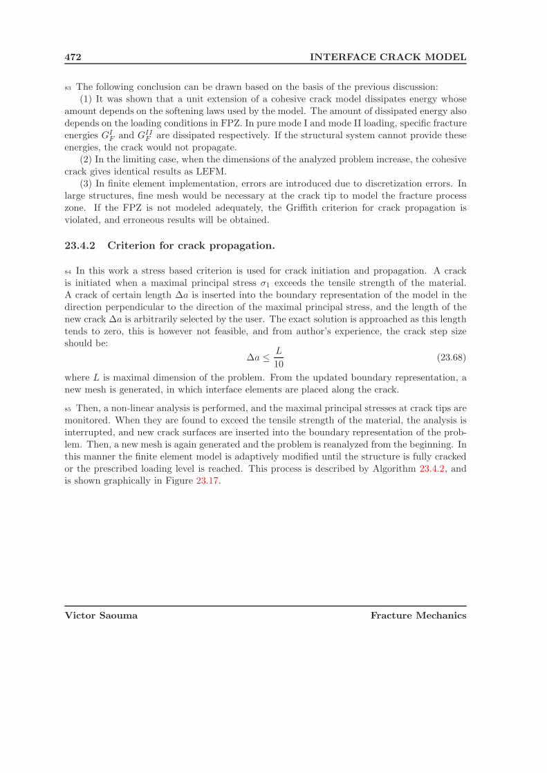
472 INTERFACE CRACK MODEL
83 The following conclusion can be drawn based on the basis of the previous discussion:(1) It was shown that a unit extension of a cohesive crack model dissipates energy whose
amount depends on the softening laws used by the model. The amount of dissipated energy alsodepends on the loading conditions in FPZ. In pure mode I and mode II loading, specific fractureenergies GI
F and GIIF are dissipated respectively. If the structural system cannot provide these
energies, the crack would not propagate.(2) In the limiting case, when the dimensions of the analyzed problem increase, the cohesive
crack gives identical results as LEFM.(3) In finite element implementation, errors are introduced due to discretization errors. In
large structures, fine mesh would be necessary at the crack tip to model the fracture processzone. If the FPZ is not modeled adequately, the Griffith criterion for crack propagation isviolated, and erroneous results will be obtained.
23.4.2 Criterion for crack propagation.
84 In this work a stress based criterion is used for crack initiation and propagation. A crackis initiated when a maximal principal stress σ1 exceeds the tensile strength of the material.A crack of certain length Δa is inserted into the boundary representation of the model in thedirection perpendicular to the direction of the maximal principal stress, and the length of thenew crack Δa is arbitrarily selected by the user. The exact solution is approached as this lengthtends to zero, this is however not feasible, and from author’s experience, the crack step sizeshould be:
Δa ≤ L
10(23.68)
where L is maximal dimension of the problem. From the updated boundary representation, anew mesh is generated, in which interface elements are placed along the crack.
85 Then, a non-linear analysis is performed, and the maximal principal stresses at crack tips aremonitored. When they are found to exceed the tensile strength of the material, the analysis isinterrupted, and new crack surfaces are inserted into the boundary representation of the prob-lem. Then, a new mesh is again generated and the problem is reanalyzed from the beginning. Inthis manner the finite element model is adaptively modified until the structure is fully crackedor the prescribed loading level is reached. This process is described by Algorithm 23.4.2, andis shown graphically in Figure 23.17.
Victor Saouma Fracture Mechanics

23.5 Examples and validation 473
[Mixed mode crack propagation.]
(1) Input: Boundary representation.
(2) Generate finite element model.
(3) Do
(3.1) Non-linear finite element analysis.
(4) While: maximal principal stresses < f ′t.
(5) If maximal principal stress exceed f ′t.
(4.1) Add new crack surfaces of length Δa tothe boundary representation in the direction perpendicular toσ1.
(4.2) Goto Step 2.
(6) Output: Boundary representation, Finite element model.
23.5 Examples and validation
86 Number of problems with known experimental or analytical results are analyzed in thissection to validate the proposed interface mode for simulating discrete fracturing along interfacesand in homogeneous concrete.
23.5.1 Direct shear test of mortar joints.
87 In this section, a nonlinear analyzes of a direct shear test with various levels of normalconfinement are presented. The experiments were performed at the University of Colorado inBoulder (Shing, Manzouri, Atkinson, Schuller and Amadei 1994) . In these experiments, a mor-tar interface between two brick was tested at three different levels of compressive confinement(150, 100 and 50 psi). Analyses are performed for these confinement values and also for zerovalue, which corresponds to a pure shear test.
88 Table 23.1 summarizes the selected material properties. Interface stiffnesses Kt and Kn
were determined by data fitting in the elastic region. The remaining interface parameters wereobtained from the experimental load-displacement curves.
89 Figure 23.19 shows a good correlation between the experimental and analytical load-displacementcurves.
Victor Saouma Fracture Mechanics

474 INTERFACE CRACK MODEL
Initial Boundary Rep.
FE Model
higher then tensile strengthPrincipal Stresses
Updated Boundary Rep.
Figure 23.17: Mixed mode crack propagation.
Victor Saouma Fracture Mechanics

23.5 Examples and validation 475
σ
Fu
2.25"
2.25"
16.86"
Figure 23.18: Schematics of the direct shear test setup.
Table 23.1: Material properties for direct shear test.Material Parameter Values
Brick
Modulus of elasticity E 800 ksiPoisson’s ratio ν 0.2
Mortar Interface
Shear stiffness Kt 600 ksi/inNormal stiffness Kn 200 ksi/inTensile strength f ′
t 50 psiCohesion c 80 psiFriction angle φf 45.0 degDilatancy angle φD 20.0 degSpecific mode I fracture energy GI
F 0.3 lbf/inSpecific mode II fracture energy GIIa
F 3.0 lbf/inStress at break point of bilinear softening law s1 12.5 psiCrack opening at break point of bilinear softening law sw1 0.0045 inCohesion at break point of bilinear softening law c1 40.0 psiCrack sliding at break point of bilinear softening law cw1 0.025 inMaximal dilatant displacement udil 0.2 in
Victor Saouma Fracture Mechanics
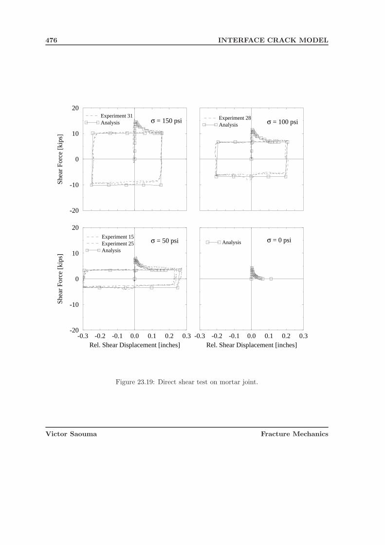
476 INTERFACE CRACK MODEL
-0.3 -0.2 -0.1 0.0 0.1 0.2 0.3Rel. Shear Displacement [inches]
-20
-10
0
10
20
Shea
r Fo
rce
[kip
s]
Experiment 15Experiment 25Analysis
-20
-10
0
10
20
Shea
r Fo
rce
[kip
s]
Experiment 31Analysis
-0.3 -0.2 -0.1 0.0 0.1 0.2 0.3Rel. Shear Displacement [inches]
Analysis
Experiment 28Analysis σ = 100 psiσ = 150 psi
σ = 50 psi σ = 0 psi
Figure 23.19: Direct shear test on mortar joint.
Victor Saouma Fracture Mechanics

23.5 Examples and validation 477
vertical Load F
F/2F/2
50 kN50 kN
135 kN135 kN
Cracksliding
Crackopening
E=23 GPa E=38 GPa
Straingages
simulated hydrostatic load
simulatedgravityload
Crack
Figure 23.20: Experimental set-up for the large scale mixed mode test.
23.5.2 Biaxial interface test.
90 The interface constitutive model described above is used to analyze the biaxial test specimenin Figure 23.20. These specimens were tested at the University of Colorado by (Saouma V.E.,and Cervenka, J. and Slowik, V. and Chandra, J.M. 1994).
91 In this first study, the material properties were optimized to yield comparable results withthe experimental ones (σt = 0.68 [MPa], c = 0.68 [MPa], φf = 30 [deg], φd = 40 [deg],GI
F = 61 [N/m], GIIF = 400 [N/m]).
92 We observe that GIF is comparable with the GF measured in wedge splitting tests on concrete,
limestone and concrete-limestone in Figure 23.2. The comparison of the numerical results withexperimental observations are shown in Figure 23.21. The numerical results show a goodagreement with the experimental ones in the peak and post-peak region.
93 In the pre-peak region, however, the initial stiffness of the specimen is overestimated. Moreanalysis and experiments are necessary to determine the reason for this discrepancy.
23.5.3 Modified Iosipescu’s beam.
94 The presented interface crack model (ICM) can also be used to model discrete cracks inhomogeneous material. This is documented on an analysis of the modified Iosipescu’s beamfrom Section ??. The geometry, boundary conditions and material properties of the problemwere discused in detail in Section ??, and hence only the aspects of the analysis directly relatedto the use of interface crack model are discussed in this section. The material properties are
Victor Saouma Fracture Mechanics

478 INTERFACE CRACK MODEL
Table 23.2: Material properties for direct shear test.Material Parameter Values
Concrete 1
Modulus of elasticity E 5.55 106 [Psi]Poisson’s ratio ν 0.18
Concrete 2
Modulus of elasticity E 3.36 106 [Psi]Poisson’s ratio ν 0.18
Interface
Shear stiffness Kt 1.887 106 [Psi/in]Normal stiffness Kn 4.453 106 [Psi/in]Tensile strength f ′
t 120 psiCohesion c 220 psiFriction angle φf 60.0 degDilatancy angle φD 45.0 degSpecific mode I fracture energy GI
F 0.35 lbf/inSpecific mode II fracture energy GIIa
F 1.05 lbf/inRatio of irreversible displacement γ 0.15Maximal dilatant displacement udil 0.5 inSoftening law for tensile strength linearSoftening law for cohesion linear
0.0 0.2 0.4 0.6 0.8CMOD [mm]
0
100
200
300
400
500
Ver
tica
l loa
d [k
N]
ExperimentAnalysis
0.00 0.10 0.20 0.30CMSD [mm]
ExperimentAnalysis
Figure 23.21: Nonlinear analysis of the mixed mode test.
Victor Saouma Fracture Mechanics

23.5 Examples and validation 479
listed in Table 23.3.
95 The label ICM indicates the material properties for the interface crack model, which is usedto simulate the fracture process zone.
Table 23.3: Material properties for ICM for Iosipescu’s test.Material Parameter Values
Concrete
Young’s modulus E 35 GPaPoisson’s ratio ν 0.15
Steel plates
Young’s modulus E 200 GPaPoisson’s ratio ν 0.22
ICM
Shear stiffness Kt 15.2 GPa/mNormal stiffness Kn 20.0 GPa/mTensile strength f ′
t 2.8 MPaCohesion c 5.0 MPaFriction angle φf 50.0 deg.Dilatancy angle φD 45.0 deg.Specific mode I fracture energy GI
F 70.0 N/mSpecific mode II fracture energy GIIa
F 700.0 N/mRatio of irreversible displacement γ 0.3Maximal dilatant displacement udil 0.01 mSoftening law for tensile strength bilinear (Wittmann & Bruhwiler)Softening law for cohesion linear
96 The model is supported at the two top plates and tractions are applied on the two bottomplates. The magnitude of the tractions is such that the total force on the left bottom steel plateis equal to 1/11 F and on the right bottom plate is 10/11 F, where F is the total force appliedin the vertical direction. The analysis is controlled by the relative sliding at the notch mouth.This means, that at each increment a unit vertical force F is applied. The applied forces arescaled to satisfy a prescribed value of the relative sliding. This displacement control scheme isdescribed in detail in (Reich 1993).
97 Two analysis were performed. In the first one, a single crack was propagated starting at thenotch. However, during this analysis, tensile principal stresses were observed along the bottomedge between the two bottom supports that were higher than the tensile strength. Therefore,a second analysis was performed, in which totally five cracks were considered.
Single crack analysis:Initially, there are no interface elements in the finite element mesh. They are inserted into
Victor Saouma Fracture Mechanics

480 INTERFACE CRACK MODEL
the model after the maximal principal stresses at the notch reach the tensile strength. Thennew crack faces are inserted into the boundary representation of the problem in the directionperpendicular to the direction of the maximal principal stress. A new finite element mesh isgenerated, and the analysis is restarted from the beginning. The analysis is stopped when themaximal principal stress at the crack tip is larger then the tensile strength. Then, again newcrack faces are inserted into the boundary representation, and a new mesh is generated. Thisprocess is repeated until the whole beam is cracked. Six different finite element meshes werenecessary in this analysis, and three of them are shown in Figures 23.22 and 23.23: the initialone, the mesh corresponding to the third step (i.e. third mesh regeneration) and the final meshwhen the crack reached the bottom edge. The crack was initiated at the notch at an angleequal to −37.3 degrees with respect to the horizontal axis. Later it curved down, and reachedthe bottom edge of the beam exactly at the right corner of the right bottom plate. Figures 23.22and 23.23 also show the positions on the load-displacement curve corresponding to each stepand the normal and shear stresses along the crack.
Multiple cracks analysis:This analysis was performed in an analogous way to the single crack one, but in the secondstep (i.e. after second remeshing), tensile stresses larger then tensile stress were observed alongthe bottom edge of the beam, therefore four additional cracks were inserted into the boundaryrepresentation at each node where the stress criterion was violated. In the subsequent step(i.e. step 4), two cracks were found to violate the stress criterion: the notch crack and the rightbottom crack. In the following non-linear analysis, however, due to the stress redistribution, thebottom cracks were unloaded, and only the notch crack propagated. Altogether, five remeshingsteps were necessary in this analysis, and some of them are shown in Figures 23.24 and 23.25.
This figures show the shaded contour areas of maximal principal stresses on the deformedshapes at steps 3,4 and 5. The finite element meshes that were used at steps 1,3,4 and 5 areillustrated in Figure 23.26.
98 The final load-displacement curves from both analyzes are shown in Figure 23.27, and canbe compared to experimental data and classical fictitious crack analysis.
99 In this figure, the label ICM indicates the results from this analysis, when the interfacecrack model was used, and the crack path was determined automatically during the analysis.The FCM label means that the classical Hillerborg fictitious model, as it was implemented by(Reich 1993) was used. In this case, the crack patch must be known or assumed, therefore, thecrack path, which was determined previously by the linear elastic fracture mechanics analysiswas used. In other words, for the case of ICM the crack path was determined automaticallyduring the nonlinear analysis, but for FCM the crack path was determined by a previous LEFManalysis (Section ??).
100 The crack paths determined by LEFM and ICM analyzes are compared in Figure 23.28.Clearly, there is almost no difference between the different crack paths, which implies thatalthough LEFM is not applicable for this problem size, it can still be used for crack patternprediction. The unsuitability of LEFM for this problem size is clearly demonstrated by the load-displacement curves in Figure ??, where the maximal peak load of about 40 kN is overestimated
Victor Saouma Fracture Mechanics

23.5 Examples and validation 481
0.0 1.0 2.0 3.0 4.0Distance from crack mouth [mm]
-1.0
0.0
1.0
2.0
3.0
σ/τ
[MP
a] στ
0.00 0.05 0.10 0.15 0.20CSD [mm]
0
10
20
30
40
50
F [
kN]
0.0 10.0 20.0 30.0Distance from crack mouth [mm]
-1.0
0.0
1.0
2.0
3.0
σ/τ
[MP
a] στ
0.00 0.05 0.10 0.15 0.20CSD [mm]
0
10
20
30
40
50
F [
kN]
Figure 23.22: Crack propagation in Iosipescu’s beam, (Steps 1 & 3).
Victor Saouma Fracture Mechanics

482 INTERFACE CRACK MODEL
0 20 40 60 80 100Distance from crack mouth [mm]
-1.0
0.0
1.0
2.0
3.0
σ/τ
[MPa
]
στ
0.00 0.05 0.10 0.15 0.20CSD [mm]
0
10
20
30
40
50
F [k
N]
0 20 40 60 80 100Distance from crack mouth [mm]
-1.0
0.0
1.0
2.0
3.0
σ/τ
[MPa
]
στ
0.00 0.05 0.10 0.15 0.20CSD [mm]
0
10
20
30
40
50
F [k
N]
Figure 23.23: Crack propagation in Iosipescu’s beam, (Increment 11 & 39 in Step 6).
Victor Saouma Fracture Mechanics
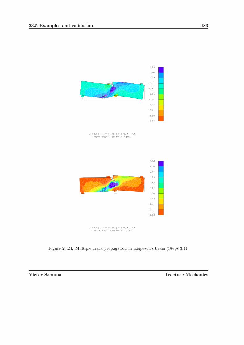
23.5 Examples and validation 483
Figure 23.24: Multiple crack propagation in Iosipescu’s beam (Steps 3,4).
Victor Saouma Fracture Mechanics

484 INTERFACE CRACK MODEL
Figure 23.25: Multiple crack propagation in Iosipescu’s beam (Step 5).
Victor Saouma Fracture Mechanics

23.5 Examples and validation 485
Figure 23.26: Meshes for crack propagation in Iosipescu’s beam (Steps 1,3,4,5).
Victor Saouma Fracture Mechanics
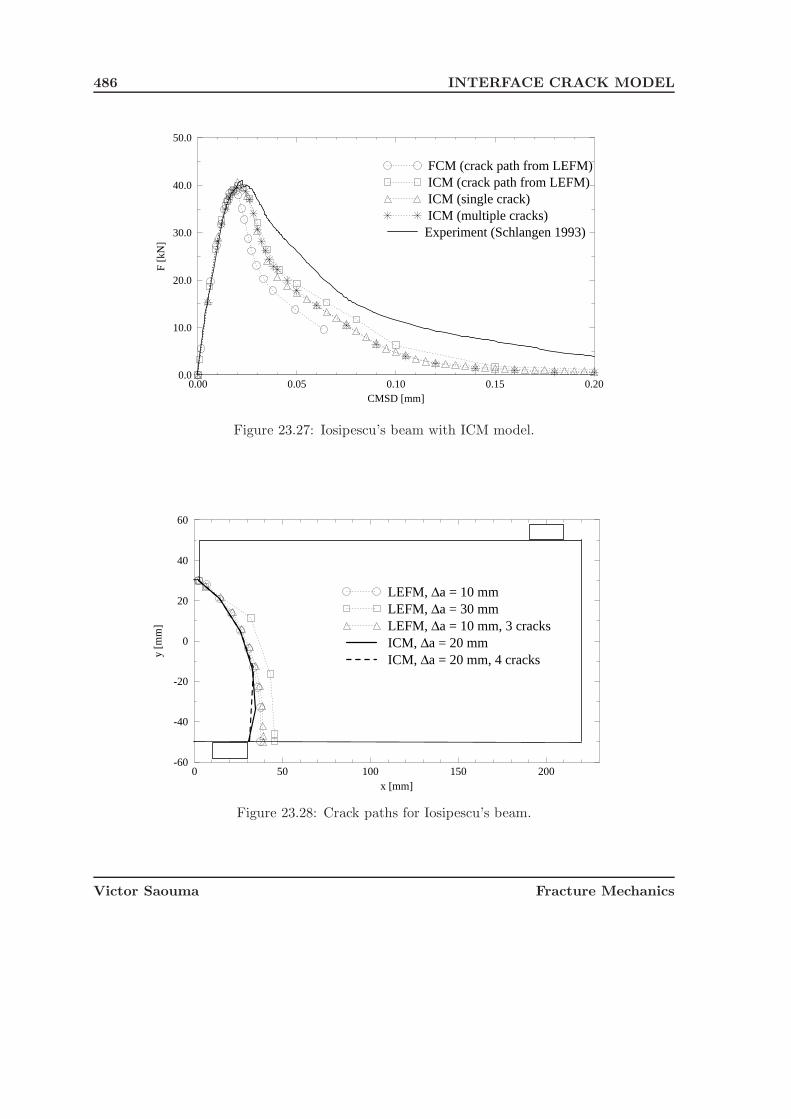
486 INTERFACE CRACK MODEL
0.00 0.05 0.10 0.15 0.20CMSD [mm]
0.0
10.0
20.0
30.0
40.0
50.0
F [k
N]
FCM (crack path from LEFM) ICM (crack path from LEFM) ICM (single crack) ICM (multiple cracks)Experiment (Schlangen 1993)
Figure 23.27: Iosipescu’s beam with ICM model.
0 50 100 150 200x [mm]
-60
-40
-20
0
20
40
60
y [m
m]
LEFM, Δa = 10 mm LEFM, Δa = 30 mm LEFM, Δa = 10 mm, 3 cracks ICM, Δa = 20 mm ICM, Δa = 20 mm, 4 cracks
Figure 23.28: Crack paths for Iosipescu’s beam.
Victor Saouma Fracture Mechanics

23.5 Examples and validation 487
by almost 100 %.
101 Theoretically, as the problem size increases, the two approaches (i.e. LEFM and ICM) shouldbecome equivalent. This is demonstrated in Figure 23.29, which shows the load displacementcurves for a specimen fifty times larger than the original one. Clearly, the two load-displacementcurves are almost identical. This example can also be considered as a proof that the ICM model
0.0 0.1 0.2 0.3 0.4 0.5 0.6 0.7 0.8CMSD [mm]
0e+00
1e+04
2e+04
3e+04
4e+04
F [k
N]
LEFM FCM (crack path from LEFM) ICM
Figure 23.29: Large Iosipescu’s beam, h = 50 x 100 mm.
approaches LEFM as the structural size encreases.
23.5.4 Anchor bolt pull-out test.
102 In Section ?? the anchor bolt pull-out experiments were analyzed using the linear elasticfracture mechanics (LEFM). LEFM is not applicable for this problem size as is documentedon the resulting load-displacement curves (Figure ??). For both geometries the loads wereoverestimated if LEFM was used. In this section, same problem is reanalyzed, but nonlinearfracture mechanics is used. The fracture process zone is modeled using the interface crackmodel developed in this chapter.
103 The problem geometry is shown in Figure ??, and material properties are listed in Table ??.
104 The finite element meshes and crack patterns for specimen type I are illustrated in Fig-ure 23.30.
105 This analysis exhibits a “zig-zag” crack pattern, which indicates that the selected crackincrement Δa of 50 mm was too large, and the crack tip “oscilates” around the correct path.Originally the crack propagated at an angle of about 20 degrees, but when the crack approachedthe support, it sharply curved down, and continued at about -55 degrees. Subsequently a
Victor Saouma Fracture Mechanics

488 INTERFACE CRACK MODEL
Figure 23.30: Crack propagation for anchor bolt pull out test I.
Victor Saouma Fracture Mechanics

23.6 Conclusions 489
secondary vertical crack developed below the vertical support causing the final failure. Eightremeshing steps were necessary in this analysis.
106 The results for specimen type II are shown in Figure 23.31, which shows the crack patternsand shaded areas of maximal principal stresses at remeshing steps 2,6,9 and 10. Altogether,ten different finite element meshes were used.
107 Two cracks were considered in this analysis. One started at the top edge of the anchorhead, and second at the bottom edge. The first crack proved to be the dominant one, and asfor specimen I, it first propagated in an almost horizontal direction (10-20 deg.), but below thesupport, the crack again sharply turned downward, and continued at the angle of approximately-45 degrees. Again, a secondary vertical crack eventually developed under the support.
108 The crack paths for both specimens are plotted in Figure 23.32, and they show a good agree-ment with the experimentally observed ones. It should be noted however that the experimentalcrack patterns in this figure are only approximate, since no quantitative data about the exactcrack patterns are reported in the literature.
109 The load-displacement curves are shown in Figure 23.33 and 23.34 for specimen I and IIrespectively. These figures show comparison of this analysis with experiments and numericalsimulations by other researchers. The experimental curves are adopted from (Shirai 1993) and(Slowik 1993) and the numerical curves correspond to the best results reported by (Shirai 1993).
23.6 Conclusions
110 In this chapter, an interface crack model was developed and applied to modeling of discretefracture of concrete, rock-concrete interfaces and masonry joints.
111 The proposed model is an extension of Hillerborg’s fictitious crack model into a more generalcase of mixed mode fracture, when shear effects must be considered.
112 The robustness of the interface constitutive algorithm is ensured by fully exploiting thegeometrical meaning of the predictor-corrector algorithm.
113 Due to the generality of the proposed model, it can be used for nonlinear fracture mechanicsof both homogeneous materials and interfaces.
114 To model mixed mode crack propagation, the model was combined with the automated meshgeneration to adaptively modify the finite element mesh to capture curve crack trajectories.
115 It was showed, that for large structures, the model approaches the linear elastic fracturemechanics solution, which implies the satisfaction of Griffith’s criterion for crack propagation,and the capability to capture size effect.
Victor Saouma Fracture Mechanics

490 INTERFACE CRACK MODEL
Figure 23.31: Crack propagation for anchor bolt pull out test II.
Victor Saouma Fracture Mechanics
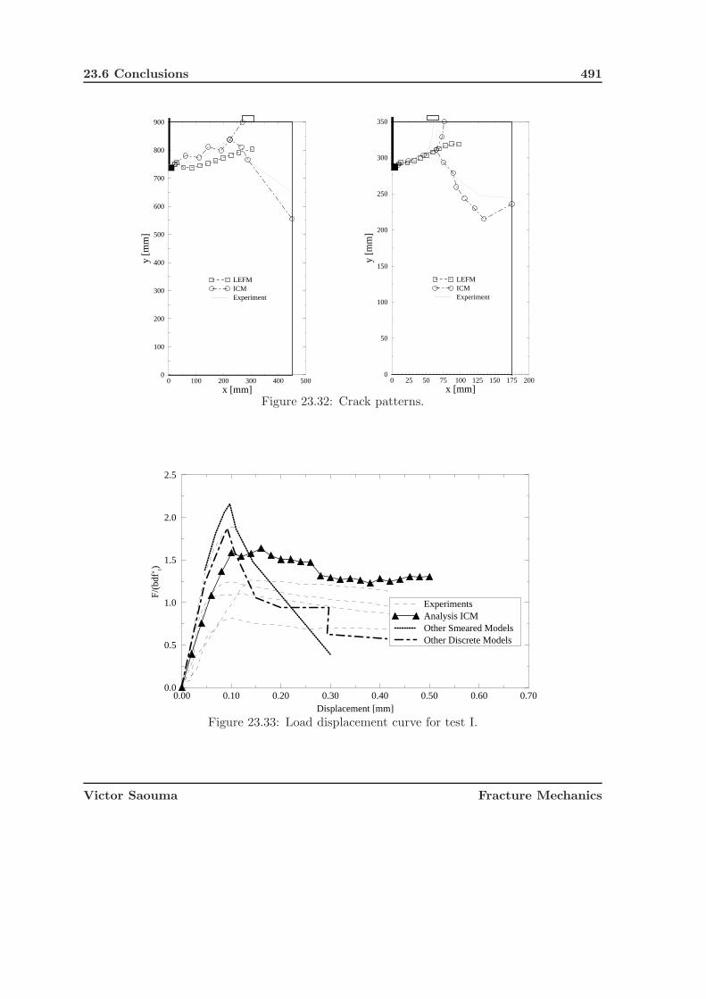
23.6 Conclusions 491
0 100 200 300 400 500x [mm]
0
100
200
300
400
500
600
700
800
900
y [m
m]
LEFM ICM Experiment
0 25 50 75 100 125 150 175 200x [mm]
0
50
100
150
200
250
300
350
y [m
m]
LEFM ICM Experiment
Figure 23.32: Crack patterns.
0.00 0.10 0.20 0.30 0.40 0.50 0.60 0.70Displacement [mm]
0.0
0.5
1.0
1.5
2.0
2.5
F/(b
df‘ t)
Experiments Analysis ICM Other Smeared Models Other Discrete Models
Figure 23.33: Load displacement curve for test I.
Victor Saouma Fracture Mechanics

492 INTERFACE CRACK MODEL
0.00 0.10 0.20 0.30 0.40 0.50 0.60 0.70Displacement [mm]
0.0
2.0
4.0
6.0
8.0
F/(b
df‘ t) Experiments (Nakajima)
Analysis, ICM Other Smeared Models Other Discrete Models
Figure 23.34: Load displacement curve for test II.
Victor Saouma Fracture Mechanics
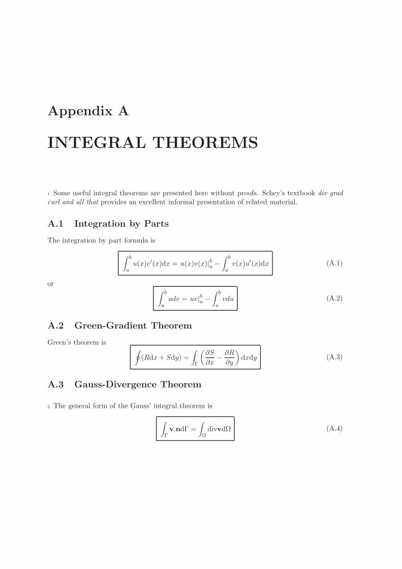
Appendix A
INTEGRAL THEOREMS
1 Some useful integral theorems are presented here without proofs. Schey’s textbook div gradcurl and all that provides an excellent informal presentation of related material.
A.1 Integration by Parts
The integration by part formula is
∫ b
au(x)v′(x)dx = u(x)v(x)|ba −
∫ b
av(x)u′(x)dx (A.1)
or ∫ b
audv = uv|ba −
∫ b
avdu (A.2)
A.2 Green-Gradient Theorem
Green’s theorem is ∮(Rdx + Sdy) =
∫Γ
(∂S
∂x− ∂R
∂y
)dxdy (A.3)
A.3 Gauss-Divergence Theorem
2 The general form of the Gauss’ integral theorem is
∫Γv.ndΓ =
∫Ω
divvdΩ (A.4)

494 INTEGRAL THEOREMS
or ∫Γ
vinidΓ =
∫Ω
vi,idΩ (A.5)
3 In 2D-3D Gauss’ integral theorem is
∫ ∫ ∫V
div qdV =
∫ ∫SqT .ndS (A.6)
or ∫ ∫ ∫V
vi,idV =
∫ ∫S
vinidS (A.7)
4 Alternatively
∫ ∫ ∫V
φdiv qdV =
∫ ∫S
φqT .ndS −∫ ∫ ∫
V(∇φ)T qdV (A.8)
5 For 2D-1D transformations, we have
∫ ∫A
div qdA =
∮sqTnds (A.9)
or ∫ ∫A
φdiv qdA =
∮sφqTnds −
∫ ∫A(∇φ)T qdA (A.10)
Victor Saouma Fracture Mechanics

Bibliography
399, A.: n.d., Standard Test Method for Plane Strain Fracture Toughness of Metallic Materials,E399–74, Annual Book of ASTM Standards.
496, A.: 2000, The Standard Test Method for Splitting Tensile Strength of Cylindrical ConcreteSpecimens, Annual Book of ASTM Standards.
Abramowitz, M. and Stegun, I.: 1970, Handbook of mathematical functions, Technical report,National Bureau of Standard. Applied Mathematics Series, No. 55.
ACI Committee 446: 1991, Fracture mechanics of concrete: Concepts, models and deformationof material properties, Technical Report ACI 446.1R-91, American Concrete Institute,Detroit, MI.
ACI Committee 446: 2003, Fracture toughness testing of concrete, Technical Report ACI446XX, American Concrete Institute, Detroit, MI.
Advani, S. and Lee, K.: 1979, Thermo-mechanical failure criteria for rock media, pp. 19–25.
Aliabadi, M. and Rooke, D.: 1991, Numerical Fracture Mechanics, Kluwer Academic Publishers.
Alvaredo, A. and Wittman, F.: 1992, Crack formation due to hygral gradients, Third Interna-tional Workshop on Behaviour of Concrete Elements Under Thermal and Hygral Gradients,Weimar, Germany.
Anderson, T.: 1995, Fracture Mechanics, Fundamentals and Applications, CRC Press.
Anon.: 1985, RILEM Draft Recommendation (50–FCM): Determination of the Fracture Energyof Mortar and Concrete by Means of Three–Point Bend Tests on Notched Beams, Materialsand Structures 18, 287–290.
Apostal, M.: 1974, Development of an Anisotropic Singularity Finite Element Utilizing theHybrid Displacement Method, PhD thesis, State University of New York.
Atkinson, C. and Bastero, J.: 1991, On the use of betti’s reciprocal theorem for computing thecoefficients of stress singularities in anisotropic media, International Journal of EngineeringScience 29(6), 727–741.

496 BIBLIOGRAPHY
Atkinson, C., Bastero, J. and Martinez-Esnaola, J.: 1988, Stress analysis in sharp angularnotches using auxiliary fields, Engineering Fracture Mechanics 31(4), 637–646.
Atkinson, C., Bastero, J. and Miranda, I.: 1986, Path-independent integrals in fracture dynam-ics using auxiliary fields, Engineering Fracture Mechanics 25(1), 53–62.
Atkinson, C. and Craster, R.: 1992, The application of invariant integrals in diffusive elasticsolids, Philosophical Transactions of the Royal Society of London, Series A 399(1653), 231–263.
Atluri, S.: 1982, Path-independent integrals in finite elasticity and inelasticity, with body forces,inertia, and arbitrary crack-face conditions, Engineering Fracture Mechanics 16(3), 341–364.
Atluri, S., Kobayachi, A. and Nakagaki, M.: 1979, Application of an assumed displace-ment hybrid finite element procedure to two dimensional problems in fracture mechanics,AIAA/ASME/SAE 15th Structures, Structural Dynamics and Materials Conference, LasVegas, Nevada.
Aviles, C. and Scholz, C.: 1987, Fractal analysis applied to characteristic segments of the sanandreas fault, Jour. Geoph. Res. 92(B1), 331–344.
Awaji, H. and Sato, S.: 1978, Combined mode fracture toughness measurement by the disctest, J. of Engrg. Mat. Tech. 100, 175–182.
Babuska, I. and Miller, A.: 1984, The post-processing approach to finite element method– partii, Int. J. Num. Meth. Engrg. 20, 1111–1129.
Balankin, A.: 1997, Physics of fracture and mechanics of self-affine cracks, Engineering FractureMechanics 57(2/3), 135–203.
Barenblatt, G.: 1962, The mathematical theory of equilibrium crack in the brittle fracture,Advances in Applied Mechanics 7, 55–125.
Barsom, J. and Rolfe, S.: 1987, Fracture & Fatigue Control in Structures, Applications ofFracture Mechanics, second Ed., Prentice-Hall.
Barsoum, R.: 1974, Application of quadratic isoparametric finite elements in linear fracturemechanics, Int. J. Fract. 10, 603–605.
Barsoum, R.: 1975, Further application of quadratic isoparametric finite elements to linearfracture mechanics of plate bending and general shells, Int. J. Fract. 11, 167–169.
Barsoum, R.: 1976a, A degenerete solid element for linear fracture analysis of plate bendingand general shells, Int. J. num. Meth. Engng. 10, 551–564.
Barsoum, R.: 1976b, On the use of isoparametric finite elements in linear fracture mechanics,Int. J. num. Meth. Engng. 10, 25–37.
Victor Saouma Fracture Mechanics

BIBLIOGRAPHY 497
Barsoum, R.: 1977, Triangular quarter point elements as elastic and perfectly plastic crack tipelements, Int. J. num. Meth. Engng. 11, 85–98.
Barsoum, R.: 1981, An assessment of the quarter-point elements in pressure vessel fractureanalysis, Structural Mechanics in Reactor Technology Conference, Paris.
Barsoum, R.: 1982, Letter to the editor, Int. J. num. Meth. Engng. 18, 1420–1422.
Barton, C., Schutter, T. and Samuel, J.: 1989, Dimension– a computer program that computesthe fractal dimension of lines or points in a plane using the box, box-rotate, box-flex, box-density, and perimeter-area methods, Technical report, United States Geological Survey,Denver, CO. Unpublished.
Bastero, J., Atkinson, C. and Martinez-Esnaola, J.: 1989, Use of path-independent integrala for mixed-mode fast crack propagation in uncoupled thermoelastic media, EngineeringFracture Mechanics 34(2), 325–335.
Batugin, S. and Nirenburg, R.: 1972, Approximate relationship among the elastic constants ofanisotropic rocks and anisotropy parameters, Fiz-Tekhn. Probl. Razrabotki Polezn. Iskopae-mykh 7(1), 7–11.
Bazant, Z. and Becq-Giraudon, E.: 2001, Estimation of fracture energy from basic characteris-tics of concrete, in R. de Borst, J. Mazars, G. Pijaudier-Cabot and J. van Mier (eds), Frac-ture Mechanics of Concrete Structures (Proc., FraMCoS-4 Int. Conf., Paris), Balkema,pp. 491–495.
Bazant, Z. and Cedolin, L.: 1991, Stability of Structures, Oxford University Press.
Bazant, Z. (ed.): 1992, Proceedings of the First International Conference on Fracture Mechanicsfor Concrete and Concrete Structures, Elsevier, Breckenridge, CO.
Bazant, Z. and Pfeiffer, P.: 1987, Determination of fracture energy properties from size effectand brittleness number, ACI Material Journal 84(6), 463–480.
Bazant, Z. and Planas, J.: 1998, Fracture and Size Effect in Concrete and Other QuasibrittleMaterials, CRC Press.
Bazant, Z., Yu, Q. and Zi, G.: 2002, Choice of standard fracture test for concrete and itsstatistical evaluation, International Journal of Fracture 118(4), 303–337.
Bazant, Z.P.: 1976, Instability, ductility and size effect in strain softening concrete, Journal ofEngng. Mech., ASCE 102(2), 331–344.
Bazant, Z.P.: 1984, Size effect in blunt fracture: Concrete, rock, metal, J. of EngineeringMechanics, ASCE 110(4), 518–535.
Bazant, Z.P: 1997, Scaling of quasibrittle fraacture: Asymptotic analysis, Int. J. of FractureMechanics 83(1), 19–40.
Victor Saouma Fracture Mechanics

498 BIBLIOGRAPHY
Bazant, Z.P.: 2002, Scaling of Structural Strength, Hermes Penton Science, London.
Bazant, Z.P.: 2005, Scaling theory for quasibrittle structural failure, Proceedings National Acad-emy of Sciences 101(37), 13397–13399.
Bazant, Z.P. and Cedolin, L.: 1979, Blunt crack propagation in finite element analysis, J. ofthe Engineering Mechanics Division, ASCE 105, 297–315.
Bazant, Z.P. and Gettu R.: 1993, Fracture of rock: Effect of loading rate, Engineering Fracturemechanics 45(3), 393–398.
Bazant, Z.P. and Kazemi, M.T.: 1990, Determination of fracture energy, process zone lengthand brittleness number from size effect, with application to rock and concrete, InternationalJournal of Fracture 44, 111–131.
Bazant, Z.P. and Novak, D.: 2000, Energetic-statistical size effect in quasibrittle failure at crackinititation, ACI Materials Journal 97(5), 381–392.
Bazant, Z.P. and Yavari, A.: 2005, Is the cause of size effect on structural strength fractal orenergetic-statistical?, Engineering Fracture Mechanics 72, 1–31.
Bazant, Z. P. and Kazemi, M.: 1990, Determination of fracture energy, process zone length andbrittleness number from size effect, with application to rock and concrete, Int. J. of Fract.44, 111–131.
Benzley, S.: 1974, Representation of singularities with isoparametric finite elements, Int. J.Num. Meth. Engng. 8, 537.
Bocca, P., Carpinteri, A. and Valente, S.: 1990, Size effects in the mixed mode crack propaga-tion: Softening and snap-back analysis, Engineering Fracture Mechanics 35(1–3), 159–170.
Bolzon, G., Fedele, R. and Maier, G.: 2002, Parameter identification of a cohesive crack modelby kalman filter, Computer Methods in Appl. Mech. Eng. 191, 2847–2871.
Bouchaud, E., Lapasset, G. and Planes, J.: 1990, Fractal dimension of fractured surfaces: auniversal value?, Europhysics Letters 13(1), 73–79.
Bourdarot, E., Mazars, J. and Saouma, V. (eds): 1994, Proceedings of the International Work-shop on Dam Fracture and Damage, Balkema.
British Standards Institution, BS 5447, London: 1977.
Broek, D.: 1986, Elementary Engineering Fracture Mechanics, 4th Edition, Martinus NijhoffPublishers.
Broek, D.: 1989, The Practical Use of Fracture Mechanics, Kluwer Academic Publishers.
Brown, S.: 1987, A note on the description of surface roughness using fractal dimension, Geo-physical Research Letters 14(11), 1095–1098.
Victor Saouma Fracture Mechanics

BIBLIOGRAPHY 499
Brown, S.: 1988, Correction to: A note on the description of surface roughness using fractaldimension, Geophysical Research Letters 15(11), 286.
Bruhwiler, E.,: 1988, Fracture Mechanics of Dam Concrete Subjected to Quasi-Static and Seis-mic Loading Conditions, Doctoral Thesis No 739, Swiss Federal Institute of Technology,Lausanne. (in German).
Bruhwiler, E.: 1992, The wedge splitting test for the determination of fracture properties,Numerical Models in Fracture Mechanics of Concrete, Proceedings of the 1st BolomeyWorkshop on Numerical Models in Fracture Mechanics of Concrete, Balkema, Zurich,Switzerland, pp. 19–27.
Bruhwiler, E., Broz, J.J., and Saouma, V.E.,: 1991, Fracture model evaluation of dam concrete,ASCE, Journal of Civil Engineering Materials 4, 235–251.
Bruhwiler, E. and Roelfstra, P.E.,: 1989, Tensile Softening Properties and Structural Responseof a Concrete Member, Proceedings, Int. Conf. on Recent Developments in the Fracture ofConcrete and Rock, University of Wales, Cardiff.
Bruhwiler, E., and Saouma, V.E.,: 1990, Fracture testing of rock by the wedge splitting test,in W. Hustrulid and G. Johnson (eds), Proceedings of the 31st US Symposium on RockMechanics, Balkema, Golden, CO, pp. 287–294.
Bruhwiler, E. and Wittmann, F.: 1990a, Failure of Dam Concrete Subjected to Seismic LoadingConditions, Engineering Fracture Mechanics 35(3), 565–572.
Bruhwiler, E. and Wittmann, F.: 1990b, The Wedge Splitting Test, a Method of PerformingStable Fracture Mechanics Tests, Engineering Fracture Mechanics 35, 117–126.
Cahn, R.: 1989, Fractal dimension and fracture, Nature 338, 201–202.
Carlsson, L. A. and Prasad, S.: 1993, Interfacial fracture of sandwich beams, EngineeringFracture Mechanics 44, 581–590.
Carol, I., Bazant, Z.P. and Prat, P.C.,: 1992, Microplane type constitutive models for distrib-uted damage and localized cracking in concrete structures, Proc. Fracture Mechanics ofConcrete Structures, Elsevier, Breckenridge, CO, pp. 299–304.
Carpinteri, A.: 1982a, Application of fracture mechanics to concrete structures, Journal ofStructural Division, ASCE 108, 833–848.
Carpinteri, A.: 1982b, Notch sensitivity in fracture testing of aggregative materials, EngineeringFracture Mechanics 16, 467–481.
Carpinteri, A.: 1986, Mechanical Damage and Crack Growth in Concrete, Martinus NijhoffPublishers.
Victor Saouma Fracture Mechanics

500 BIBLIOGRAPHY
Carpinteri, A.: 1994, Scaling laws and renormlaization groups for strength and toughness dis-ordered materials, Int. J. of Solids and Structures 31(3), 291–302.
Carpinteri, A. and Chiaia, B.: 1994, Multifractal scaling law for the fracture energy variationof concrete structures, in W. F.H. (ed.), Proceedings of Second International Conferenceon Fracture Mechanics of Concrete Structures FraMCoS2, Aedificato, Zurich, Switzerland,pp. 581–596.
Carpinteri, A., Chiaia, B. and Cornetti, P.: 2003, On the mechanics of quasi-brittle materialswith a fractal microstructure, Engineering Fracture Mechanics 70, 2321–2349.
Carpinteri, A., Chiaia, B. and Ferro, G.: 1995, Size effects on nominal tensile strength ofconcrete strucutres: Multifractality of material ligaments and dimensional transition fromorder to disorder, Materials and Structures 28, 311–317.
Carpinteri, A. and Ingraffea, A. (eds): 1984, Fracture Mechanics of Concrete: Material Char-acterization and Testing, Martinus Nijhoff Publishers.
Cedolin, L., Dei Poli, S. and Iori, I.: 1987, Tensile behavior of concrete, J. of EngineeringMechanics, ASCE 113(3).
Chandra, K. and Saouma, V.: 2004, Fracture of rock-concrete interfaces: Laboratory tests andapplications, ACI Structural Journal 101(3).
Chelidze, T. and Gueguen, Y.: 1990, Evidence of fractal fracture, Int. J. Rock Mech. Min. Sci.& Geomech. Abstr. 27(3), 223–225.
Chen, C. and Runt, J.: 1989, Fractal analysis of polystrene fracture surfaces, Polymer Com-munications 30, 334–335.
Cherepanov, G.: 1979, Mechanics of Brittle Fracture, McGraw-Hill.
Comninou, M.: 1977, The interface crack, ASME, Journal of Applied Mechanics pp. 631–636.
Cottrell, A.: 1963.
Crisfield, M.A.: 1981, A fast incremental/iterative solution procedure that handles ‘snapthrough’, Computers and Structures 13(1-3), 55–62.
Crisfield, M.A.: 1991, Non-linear Finite Element Analysis of Solids and Structures, Vol 1, JohnWilley & Sons.
Cusatis, G., Bazant, Z. and Cedolin, L.: 2003, Confinement-shear lattice model for concretedamage in tension and compression: I. theory, ASCE Journal of Engineering Mechanics129(12), 1439–1448.
Dahlblom, O. and Ottosen, N. S.: 1990, Smeared crack analysis using a generalized fictitiouscrack model, Journal of Engineering Mechanics 116(1), 55–76.
Victor Saouma Fracture Mechanics
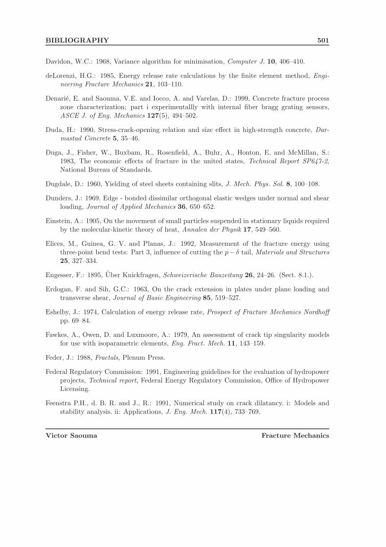
BIBLIOGRAPHY 501
Davidon, W.C.: 1968, Variance algorithm for minimisation, Computer J. 10, 406–410.
deLorenzi, H.G.: 1985, Energy release rate calculations by the finite element method, Engi-neering Fracture Mechanics 21, 103–110.
Denarie, E. and Saouma, V.E. and Iocco, A. and Varelas, D.: 1999, Concrete fracture processzone characterization; part i experimentallly with internal fiber bragg grating sensors,ASCE J. of Eng. Mechanics 127(5), 494–502.
Duda, H.: 1990, Stress-crack-opening relation and size effect in high-strength concrete, Dar-mastad Concrete 5, 35–46.
Duga, J., Fisher, W., Buxbam, R., Rosenfield, A., Buhr, A., Honton, E. and McMillan, S.:1983, The economic effects of fracture in the united states, Technical Report SP647-2,National Bureau of Standards.
Dugdale, D.: 1960, Yielding of steel sheets containing slits, J. Mech. Phys. Sol. 8, 100–108.
Dunders, J.: 1969, Edge - bonded dissimilar orthogonal elastic wedges under normal and shearloading, Journal of Applied Mechanics 36, 650–652.
Einstein, A.: 1905, On the movement of small particles suspended in stationary liquids requiredby the molecular-kinetic theory of heat, Annalen der Physik 17, 549–560.
Elices, M., Guinea, G. V. and Planas, J.: 1992, Measurement of the fracture energy usingthree-point bend tests: Part 3, influence of cutting the p− δ tail, Materials and Structures25, 327–334.
Engesser, F.: 1895, Uber Knickfragen, Schweizerische Bauzeitung 26, 24–26. (Sect. 8.1.).
Erdogan, F. and Sih, G.C.: 1963, On the crack extension in plates under plane loading andtransverse shear, Journal of Basic Engineering 85, 519–527.
Eshelby, J.: 1974, Calculation of energy release rate, Prospect of Fracture Mechanics Nordhoffpp. 69–84.
Fawkes, A., Owen, D. and Luxmoore, A.: 1979, An assessment of crack tip singularity modelsfor use with isoparametric elements, Eng. Fract. Mech. 11, 143–159.
Feder, J.: 1988, Fractals, Plenum Press.
Federal Regulatory Commission: 1991, Engineering guidelines for the evaluation of hydropowerprojects, Technical report, Federal Energy Regulatory Commission, Office of HydropowerLicensing.
Feenstra P.H., d. B. R. and J., R.: 1991, Numerical study on crack dilatancy. i: Models andstability analysis. ii: Applications, J. Eng. Mech. 117(4), 733–769.
Victor Saouma Fracture Mechanics
502 BIBLIOGRAPHY
Foreman, R., Kearney, V. and Engle, R.: 1967, Numerical analysis of crack propagation incyclic-loaded structures, J. of Basic Engineering 89, 459–464.
Freese, C. and Tracy, D.: 1976, The natural isoparametric triangle versus collapsed quadrilateralfor elastic crack analysis, Int. J. Fract. 12, 768–770.
Galilei, G.: 1638, Dialogues Concerning Two New Sciences, Dover Publications (1954), NewYork, NY. Originally published by Elzevir, The Neterlands, 1638.
Gallagher, R.: 1975, Finite Element Analysis Fundamentals, Prentice Hall, Englewood Cliffs,N.J.
Gdoutos, E.: 1993, Fracture Mechanics; An Introduction, Kluwer Academic Press.
Gerstle, W. and Xie, M.: 1992, Fem modeling of fictitious propagation in concrete, Journal ofEngineering Mechanics 118(2), 416–434.
Giuriani, E. and Rosati, G. P.: 1986, Behaviour of concrete elements under tension after crack-ing, Studi e Ricerche, Corso di Perfezionamento per le Costruzioni in Cemento Armato8, 65–82. (in Italian).
Goodman, R.E., Taylor, R.C. and Brekke, T.C.,: 1968, A Model for the Mechanics of JointedRocks, J. of the Soil Mechanics and FOundations Division ASCE 94, 637–659.
Gopalaratnam, V. S. and Shah, P. S.: 1985, Softening response of plain concrete in directtension, ACI Journal 82, 310–323.
Gopalaratnam, V. S. and Ye, B. S.: 1991, Numerical characterization of the nonlinear fractureprocess in concrete, Engineering Fracture Mechanics 40(6), 991–1006.
Gordon, J.: 1988, The Science of Structures and Materials, Scientific American Library.
Griffith, A.: 1921, The phenomena of rupture and flow in solids, Phil. Trans. Roy. Soc. LondonA221, 163–197.
Guinea, G., Pastor, J., Planas, J. and Elices, M.: 1998, Stress intensity factor, compliance andcmod for general three-point-bend-beam, International Journal of Fracture 89, 103–116.
Harrop, L.: 1982, The optimum size of quarter-point crack tip element, Int. J. num. Meth.Engng. 17, 1101–1103.
He, M. Y. and Hutchinson, J. W.: 1989, Kinking of a crack out of an interface, Journal ofApplied Mechanics 56, 270–278.
Hellen, T.: 1975, On the method of virtual crack extension, Int. J. Num. Methods in Eng. 9(1).
Hellen, T. and Blackburn, W.: 1975a, The calculation of stress intensity factor for combinedtensile and shear loading, Int. J. Fract. 11, 605–617.
Victor Saouma Fracture Mechanics

BIBLIOGRAPHY 503
Hellen, T. K. and Blackburn, W. S.: 1975b, The calculation of stress intensity factors forcombined tensile and shear loading, International Journal of Fracture 11(4), 605–617.
Henshell, R. D. and Shaw, K. G.: 1975, Crack tip elements are unnecessary, InternationalJournal of Numerical Methods in Engineering 9(3), 495–509.
Heping, X.: 1987, The fractal effect of irregularity of crack branching on the fracture toughnessof brittle materials, International Journal of Fracture 41, 267–274.
Hibbitt, H.: 1977, Some properties of singular isoparametric elements, Int. J. num. Meth.Engng. 11, 180–184.
Hillerborg, A.: 1983, Analysis of One Single Crack, in F. Whittman (ed.), Fracture Mechanics ofConcrete, F.H. Wittmann (editor), Elsevier, Amsterdam, The Netherlands, pp. 223–249.
Hillerborg, A.: 1985, The Theoretical Basis of a Method to Determine the Fracture energy GF
of Concrete, RILEM Materials and Structures 18(106), 291–296.
Hillerborg, A.: 1985a, Results of three comparative test series for determining the fractureenergy gf of concrete, Mater. and Struct. 18(107).
Hillerborg, A.: 1985b, The theoretical basis of method to determine the fracture energy gf ofconcrete, Materials and Structures 18(106), 291–296.
Hillerborg, A. and Modeer, M. and Petersson, P.E.: 1976a, Analysis of crack formation andcrack growth in concrete by means of fracture mechanics and finite elements, Cement andConcrete Research 6(6), 773–782.
Hillerborg, A. and Modeer, M. and Petersson, P.E.: 1976b, Analysis of crack formation andcrack growth in concrete by means of fracture mechanics and finite elements, Cement andConcrete Research 6(6), 773–782.
Hong, C.-C. and Stern, M.: 1978, The computation of stress intensity factors in dissimilarmaterials, Journal of Elasticity 8(1), 21–34.
Hordijk, D., Reinhardt, H. and Cornelissen, H.: 1989, Fracture mechanics parameters ofconcrete from uniaxial tensile tests as influenced by specimen length, in S. Shah andS. Swartz (eds), RILEM-SEM Int. Conference on Fracture Mechanics of Rock and Con-crete, Springer-Verlag, New-York.
Hudson, C. and Seward, S.: 1978, A Compendium of Sources of Fracture Toughness and FatigueCrack Growth Data for Metallic alloys, Vol. 14, Int. J. of Fracture.
Hudson, C. and Seward, S.: 1982, A compendium of sources of fracture toughness and fatiguecrack growth data for metallic alloys, Int. J. of Fracture, Part II 20, R59–R117.
Hurst, H.: 1951, Long-term sorage capacity of reservoirs, Trans. Am. Soc. Civ. Eng. 116, 770–808.
Victor Saouma Fracture Mechanics

504 BIBLIOGRAPHY
Hussain, M., Pu, S. and Underwood, J.: 1974, Strain energy release rate for a crack undercombined mode i and mode ii, ASTM, STP 560 pp. 2–28.
Hussain, M., Vasilakis, J. and Pu, L.: 1981, Quadratic and cubic transition elements, Int. J.Num. Meth. Engng. 16, 1397–1406.
Hutchinson, J.: 1968, Singular behavior at the end of a tensile crack tip in a power-law hardeningmaterial, Journal of Mechanics and Physics of Solids 16, 13–31.
Hutchinson, J. W. and Suo, Z.: 1992, Mixed mode cracking in layered materials, Advances inApplied Mechanics 29, 63–191.
Il’yushin, A.: 1946, The theory of small elastic-plastic deformations, Prikadnaia Matematika iMekhanika, PMM 10, 347–356.
Inglis, C.: 1913, Stresses in a plate due to the presence of cracks and sharp corners, Trans. Inst.Naval Architects 55, 219–241.
Ingraffea, A.: 1977, Discrete Fracture Propagation in Rocks: Laboratory Tests and Finite Ele-ment Analysis, PhD thesis, University of Colorado.
Ingraffea, A. and Gerstle, W.: 1984, Non-linear fracture models for discrete crack propagation,in S. Shah (ed.), Proceedings of the NATO Advanced Workshop on Application of FractureMechanics to Cementitious Composites, Martinus Nijhoff, Hingham, Mass, pp. 171–209.
Ingraffea, A. and Manu, C.: 1980, Stress intensity factor computation in three dimension withquarter-point elements, Int. J. num. Meth. Engng. 15(10), 1427–1445.
International Conference on Fracture and Damage of Concrete and Rock: 1988, Vienna. To bePublished in Engineering Fracture Mechanics.
Irwin, G.: 1957, Analysis of stresses and strains near the end of a crack traversing a plate,Transactions ASME, J. Appl. Mech. 24.
Irwin, G.: 1960, Plastic zone near a crack and fracture toughness, Proc. 7th Sagamore Conf.,p. 63.
Irwin, G.: 1962, The crack extension force for a part through crack in a plate, TransactionsASME, J. Appl. Mech. 29.
Ishikawa, H.: 1980, A finite element analysis of stress intensity factors for combined tensile andshear loading by only a virtual crack extension, Int. J. Fracture 16, 243.
Issa, M., Hammad, A. and Chudnovsky, A.: 1993, Correlation between crack tortuosity andfracture toughness in cementitious materials, International Journal of Fracture 60, 97–105.
Izquierdo-Encarnacion, J.: 2003, Ars sine scientia nihil est, Concrete International 25(5), 7.
Victor Saouma Fracture Mechanics

BIBLIOGRAPHY 505
Jeang, F. L. and Hawkins, N. M.: 1985, Nonlinear analysis of concrete fracture, Structures andmechanics report, Department of Civil Engineering, University of Washington, Seattle,WA.
Jenq, Y. and Shah, S. P.: 1985, A two parameter fracture model for concrete, Journal ofEngineering Mechanics Division, ASCE 111(4), 1227–1241.
Kanninen, M.: 1984, Applications of fracture mechanics to fiber composite materials and adhe-sive joint, a review, 3rd Int. Conf. on Numerical Methods in Fracture Mechanics, Swansea.
Kanninen, M. and Popelar, C.: 1985, Advanced Fracture Mechanics, Oxford University Press.
Kaplan, M.: 1961, Crack propagation and the fracture of concrete, Journal of the AmericanConcrete Institute 58(5), 591–610.
Karihaloo, B.: 1996, Physical causes for size effect in concrete structures, in A. Carpinteri (ed.),Size-Scale Effects in the Failure Mechanisms of Materials and Structures, E. & FN Spon,London, pp. 325–339.
Karihaloo, B.: 1999, Size effect in shallow and deep notched quasi-brittle structures, Inter-national Journal of Fracture 95, 379–390. Special issue on Fracture Scaling ed. by Z.P.Bazant and Y.D.S. Rajakapse.
Karihaloo, B. L. and Nallathambi, P.: 1987, Notched beam test: Mode i fracture toughness,Technical report, draft report to RILEM Committee 89-FMT, Fract. Mech. of Concrete:Test Method.
Karlsson, A. and Backlund, J.: 1978, J-integral at loaded crack surfaces, International Journalof Fracture 14(6), R311–R314.
Kelly, A.: 1974, Strong Solids, second edn, Oxford University Press.
Knott, J.: 1976, Fundamentals of Fracture Mechanics, fourth edn, Butterworths.
Knowles, J. and Stenberg, E.: 1972, On a class of conservation laws in linearized and finiteelastostatics, Arch. Rat. Mech. Anal. 44, 187–211.
Knowles, J. and Sternberg, E.: 1972, On a class of conservation laws in linearised and finiteelastostatics, Arch. Rat. Mech. Anal. 44, 187–211.
Koch, H. v.: 1904, Sur une Courbe Continue sans Tangente, Obtenue par une ConstructionGeometrique Elementaire, Archiv for Matemat., Astron. och Fys 1, 681–702.
Kreyszig, E.: 1979, Advanced Engineering Mathematics, 4 th Edition, John Wiley and Sons.
Kumar, V., German, M. and Shih, C.: 1981, An Engineering Approach for Elastic-PlasticFracture Analysis, Electric Power Research Institute. EPRI-NP1931.
Victor Saouma Fracture Mechanics

506 BIBLIOGRAPHY
Lange, D., Jennings, H. and Shah, S.: 1993, Relationship between fracture surface roughnessand fracture behavior of cement paste and mortar, Journal of the American CeramicSociety 76(3).
Lekhnitskii, S.: 1981, Theory of Elasticity of an Anisotropic Body, Mir, Moscow (EnglishTranslation).
Lenke, L. and Gerstle, W.: 2001, Tension test of stress versus crack opening displacement usingcylindrical concrete specimens, in C. Vipulanandan and W. Gerstle (eds), Fracture Me-chanics for Concrete Materials: Testing and Applications, pp. 189–206. SP-201, AmericanConcrete Institute, Farmington Hills, Michigan.
Levi, B.: 1990, Are fractures fractal or quakes chaotic, Physics Today pp. 17–19.
Li, F. Z. and Shih, C. F. and Needleman, A.: 1985, A comparison of methods for calculatingenergy release rates, Engineering Fracture Mechanics 21(2), 405–421.
Li, V. C. and Liang, E.: 1986, Fracture processes in concrete and fiber reinforced cementitiouscomposites, Journal of Engineering Mechanics, ASCE 112(6), 566–586.
Lin, K. Y. and Mar, J. W.: 1976, Finite element analysis of stress intensity factors for cracksat a bi-material interface, Int. Journal of Fracture 12, 521–531.
Linsbauer, H. and Tschegg, E.: 1986, Test Method for the Determination of Fracture MechanicsProperties. Austrian Patent No. A-233/86 (in German).
Long, Q., Suqin, L. and Lung, C.: 1991, Studies on the fractal dimension of a fracture surfaceformed by slow stable crack propagation, Journal of Physics, D 24(4).
Lotfi, H.: 1992, Finite Element Analysis of Fracture of Concrete and Masonry Structures, PhDthesis, University of Colorado, Boulder.
Lynn, P. and Ingraffea, A.: 1977, Transition elements to be used with quarter-point crack-tipelements, Int. J. num. Meth. Engng. 11, 1031–1036.
Malyshew, B. M. and Salganik, R. L.: 1965, The strength of adhesive joints using the theoryof cracks, Int. Journal of Fracture 1, 114–118.
Mandelbrot, B.: 1983, The Fractal Geometry of Nature, W.H. Freeman, San Francisco.
Mandelbrot, B., Passoja, D. and Paullay, A.: 1984, Fractal character of fracture surfaces ofmetals, Nature 308, 721–722.
Mecholsky, J. and Freiman, S.: 1991, Relationship between fractal geometry and fractography,Journal of the American Ceramic Society 74(12), 3136–3138.
Mecholsky, J. and Mackin, T.: 1988, Fractal analysis of fracture in ocala chert, Journal ofMaterials Science Letters 7, 1145–1147.
Victor Saouma Fracture Mechanics

BIBLIOGRAPHY 507
Mecholsky, J., Passoja, D. and Feinberg-Ringle, K.: 1989, Quantitative analysis of brittlefracture surfaces using fractal geometry, Jour. Amer. Ceram. Soc. 72(1), 60–65.
Miller, M. and Gallagher, J.: 1981, An analysis of several fatigue crack growth rate (fcgr)descriptions, in S. Hudak Jr. and R. Bucci (eds), Fatigue Crack Growth Measurements andData Analysis, ASTM STP 738, ASTM, Philadelphia, pp. 205–251.
Mindess, S. and Young, F.: 1981, Concrete, Prentice-Hall, Inc.
Maløy, K., Hansen, A., Hinrichsen, E. and Roux, S.: 1992, Experimental measurements of theroughness of brittle cracks, Physical Review Letters 68(2), 213–215.
Mosolov, A.: 1991, Fractal j integral in fracture, Soviet Technical Physics Letters 17(10), 698–700.
Mostovoy, e. a.: 1967, Use of crack-line loaded specimens for measuring plane strain fracturetoughness, J. of Materials 2(3), 661–681.
Murakami, Y.: 1987, Stress Intensity Factors Handbook, Pergamon Press. (2 Vols).
Nakayama, J.: 1965, Direct measurement of fracture energies of brittle heterogeneous material,J. of the Amer. Ceram. Soc. 48(11).
Nallathambi, P. and Karihaloo, B.: 1986, Stress intensity factor and energy release rate forthree-point bend specimens, Magazine of Concrete Research 38(135), 67–76.
Newman, J.: 1971, An improved method of collocation for the stress analysis of cracked plateswith various shaped boundaries, Technical Report NASA TN D-6376, National Aeronauticsand Space Administration, Langley Research Center, Hampton, VA.
Newman, J. and Raju, I.: 1981, An emperical stress intensity factor equation for surface cracks,Engineering Fracture Mechanics 15, 185–192.
Newton, R.: 1973, Degeneration of brick-type isoparametric elements, Int. J. num. Meth. En-gng. 7, 579–581.
Nikishkov, G. P. and Atluri, S. N.: 1987, Calculation of fracture mechanics parameters for an ar-bitrary three-dimensional crack, by the ‘equivalent domain integral’ method, InternationalJournal of Numerical Methods in Engineering 24(9), 1801–1821.
Nikishkov, G. and Vainshtok, V.: 1980, Method of virtual crack growth for determining stressintensity factors ki and kII , Strength of Materials 12, 696–701.
Ouchterlony, F.: 1982, Fracture toughness testing of rock, Technical report, SveDeFo, SwedishDetonic Research Foundation, Stockholm, Sweden.
Ouchterlony, F.: 1986, Suggested methods for determining fracture toughness of rock mate-rial, Technical report, International Society for Rock Mechanics, Commission on TestingMethods.
Victor Saouma Fracture Mechanics

508 BIBLIOGRAPHY
Owen, D. and Fawkes, A.: 1983, Engineering Fracture Mechanics, Pineridge Press, Swansea,U.K.
Paris, P. and Erdogan, F.: 1963, A critical analysis of crack propagation laws, J. of BasicEngineering, ASME 85(3), 528.
Parks, D.: 1974, A stiffness derivative finite element technique for determination of crack tipstress intensity factors, Int. J. Fracture 10, 487–502.
Peng, G. and D., T.: 1990, The fractal nature of a fracture surface, Journal of Physics A:Mathematical and General 23, 3257–3261.
Petersson, P.: 1981, Crack growth and development of fracture zones in plain concrete andsimilar materials, Technical Report TVBM 1006, Lund Institute of Technology, Lund,Sweden.
Planas, J. and Elices, M.: 1988a, Conceptual and experimental problems in the determinationof the fracture energy of concrete, Workshop on Fracture Toughness and Fracture Energy,Test Methods for Concrete and Rock, Tohoku Univ., Sendai, Japan, pp. 203–212.
Planas, J. and Elices, M.: 1988b, Size-effect in concrete structures: mathematical approxi-mations and experimental validation, in J. Mazars and Z. Bazant (eds), Cracking andDamage, Strain Localization and Size Effect, Cachan (F), pp. 462–476.
Planas, J. and Elices, M.: 1992, Asymptotic analysis of a cohesive crack: 1. theoretical back-ground, International Journal of Fracture 55, 153–177.
Planas, J., Guinea, G. V. and Elices, M.: 1999, Size effect and inverse analysis in concretefracture, International Journal of Fracture 95, 367–378.
Pu, S., Hussain, M. and Lorensen, W.: 1977, Collapsed 12 node triangular elements as cracktip elements for elastic fracture, Technical report, Tech. Rep. ARLCB-TR-77047.
Rao, A. K., Raju, I. and Krishna Murty, A.: 1971, A powerful hybrid method in finite elementanalysis, Int. J. Num. Meth. Engng. 3.
Reich, R.: 1993, On the Marriage of Mixed Finite Element Methods and Fracture Mechanics:An Application to Concrete Dams, PhD thesis, University of Colorado, Boulder.
Rice, J. R.: 1988, Elastic fracture mechanics concepts for interfacial cracks, ASME, Journal ofApplied Mechanics 55, 98–103.
Rice, J. and Sih, G.: 1965, Plane problems of cracks in dissimilar media, J. Applied Mechanicspp. 418–423.
RILEM Committee on Fracture Mechanics of Concrete - Test Methods: 1985, Determination ofthe fracture energy of mortar and concrete by means of three-point bend tests on notchedbeams, Materials and Structures 18(106), 285–290.
Victor Saouma Fracture Mechanics

BIBLIOGRAPHY 509
RILEM Committee on Fracture Mechanics of Concrete-Test Methods: 1990, Determination offracture parameters (kIc and ctodc) of plain concrete using three point bend tests, Materialsand Structures 23, 457–460.
RILEM TC QFS: 2004, Quasibrittle fracture scaling and size effect, Materials and Structures37(272), 547–568.
Roelfstra, P. and Sadouki, H.: 1986, Fracture/1: Theory and applications, Laboratory forBuilding Materials (LMC), EPF Lausanne .
Rooke, D. and Cartwright, D.: 1976, Compendium of Stress Intensity Factors, HMSO, London.
Saouma, V., Ayari, M. and Leavell, D.: 1987, Mixed mode crack propagation in homogeneousanisotropic solids, Engineering Fracture Mechanics 27(2), 171–184.
Saouma, V. and Barton, C.: 1994, Fractals, fractures and size effects in concrete, Journal ofEngineering Mechanics of the American Society of Civil Engineers 120(4), 835–854.
Saouma, V., Broz, J., Bruhwiler, E. and Boggs, H.: 1991, Effect of aggregate and specimen sizeon fracture properties of dam concrete, ASCE, Journal of Materials in Civil Engineering3(3), 204–218.
Saouma, V., Dungar, R. and Morris, D. (eds): 1991, Proceedings Dam Fracture, Electric PowerResearch Institute (EPRI), Palo Alto, CA, Boulder.
Saouma, V., Natekar, D. and Hansen, E.: 2003, Cohesive stresses and size effects in elasto-plastic and quasi-brittle materials, International Journal of Fracture 119, 287–298.
Saouma, V., Natekar, D. and Sbaizero, O.: 2002, Nonlinear finite element analysis and sizeeffect study of a metal-reinforced ceramics-composite, Materials Science and EngineeringA 323, 129–137.
Saouma, V. and Schwemmer, D.: 1984, Numerical evaluation of the quarter point singularelement, International Journal of Numerical Methods in Engineering 20, 1629–1641.
Saouma, V. and Sikiotis, E.: 1986, Stress intensity factors in anisotropic bodies using singularisoparametric elements, Engineering Fracture Mechanics 25(1), 115–121.
Saouma, V., Cervenka, J. and Reich, R.: 1997–2004, Merlin, a three-dimensional finite elementprogram based on a mixed-iterative solution strategy for problems in elasticity, plastic-ity, and linear and nonlinear fracture mechanics; user’s manual, Technical report, Elec-tric Power Research Institute (EPRI), Palo Alto; Tokyo Electric Power Service Company(TEPSCO), Tokyo. http://civil.colorado.edu/~saouma/Merlin.
Saouma, V. and Zatz, I.: 1984, An automated finite element procedure for fatigue crack prop-agation analyses, Engineering Fracture Mechanics Journal 20(2), 321–333.
Victor Saouma Fracture Mechanics

510 BIBLIOGRAPHY
Saouma, V.E., Barton, C., and Gamal-El-Din, N.: 1990, Fractal Characterization of CrackedConcrete Surfaces, Engineering Fracture Mechanics Journal 35(1), 47–53.
Saouma V.E., and Cervenka, J. and Slowik, V. and Chandra, J.M.: 1994, Mixed mode frac-ture of rock-concrete interfaces, in Z. Bazant (ed.), US-Europe Workshop on Fractureand Damage of Quasi-Brittle Materials: Experiment, Modeling and Computer Analysis,Prague, Czech Republic.
Schertzer, D. and Lovejoy, S.: 1997, Universal multifractals do exist!: Comments on a statis-tical analysis of mesoscale rainfall as a random cascade, Journal of Applied Meteorology36, 1296–1303.
Sha, G.: 1984, On the virtual crack extension technique for stress intensity factors and energyrelease rate calculation for mixed fracture modes, Int. J. Fracture 25.
Shah, S. (ed.): 1984, Application of Fracture Mechanics to Cementitious Composites, North-western University. NATO Workshop.
Shah, S. and Swartz, S. (eds): 1989, RILEM-SEM Int. Conference on Fracture Mechanics ofRock and Concrete, Springer-Verlag, New-York.
Shih, C., de Lorenzi, H. and German, M.: 1976, Crack extension modelling with singularquadratic isoparametric elements, Int. J. Fract. 12, 647–651.
Shih, C., Moran, B. and Nakamura, T.: 1986, Energy release rate along a 3-d crack front in athermally stressed body, Int. J. Fracture 30, 79–102.
Shing, P., Manzouri, T., Atkinson, R., Schuller, M. and Amadei, B.: 1994, Evaluation of groutinjection techniques for unreinforced masonry structures, Proc. of the Fifth U.S. NationalConference on Earthquake Engineering, Vol. III, Chicago, pp. 851–860.
Shirai, N.: 1993, Jci round robin analysis in size effect in concrete structures, US-Japan Work-shop on Fracture and Size Effect in Concrete, Japan.
Sierpinski, W.: 1912, Sur une nouvelle courbe continue qui remplit toute une aire plane., Bull.l’Acad. des Sciences Cracovie A pp. 462–478.
Sih, G.: 1974, Strain energy factors applied to mixed mode crack problems, Int. J. Fracture10, 305.
Sih, G. and DiTommaso, A. (eds): 1984, Fracture Mechanics of Concrete: Structural Applica-tion and Numerical Calculation, Martinus Nijhoff Publishers.
Sih, G., Paris, P. and Irwin, G.: 1965, On cracks in rectilinearly anisotropic bodies, InternationalJournal of Fracture Mechanics 1.
Victor Saouma Fracture Mechanics

BIBLIOGRAPHY 511
Slowik, W.: 1993, Beitrage zur Experimentellen Bestimmung Bruchmechanisher Materialpa-rameter von Betonen, Technical report, Institut fur Baustoffe, ETH, Zurich, Switzerland.Research Report No. 3.
Sluys, L.: 1992, Wave Propagation, Localisation and Dispersion of Softening Solids, PhD thesis,Delft University of Technology.
Sokolnikoff, I.: 1956, Mathematical Theory of Elasticity, McGraw-Hill, New York, NY.
Stankowski, T.: 1990, Numerical Simulation of Progressive Failure in Particle Composites, PhDthesis, University of Colorado, Boulder.
Stern, M.: 1973, A boundary integral representation for stress intensity factors, in T. S. Chang(ed.), Recent Advances in Engineering Science, Scientific Publishers, Boston, MA, pp. 125–132. Volume 7.
Stern, M.: 1979, The numerical calculation of thermally induced stress intensity factors, Journalof Elasticity 9(1), 91–95.
Stern, M., Becker, E. and Dunham, R.: 1976, A contour integral computation of mixed modestress intensity factors, International Journal of Fracture 12(3), 359–368.
Stern, M. and M.L., S.: 1975, The calculation of stress intensity factors in anisotropic materialsby a contour integral mehtod, in R. E.F. and S. Benzley (eds), Computational FractureMechanics, ASME, New York, NY, pp. 161–171.
Stevens, R. and Guiu, F.: 1994, The application of the j integral to problems of crack bridging,Acta Metall. Mater 42(6), 1805–1810.
Swartz, S. E. and Go, C. G.: 1984, Validity of compliance calibration to cracked concrete beamsin bending, Exp. Mech. 24(2), 129–134.
Swartz, S. E., Hu, K. K., Fartash, M. and Huang, C. M. J.: 1982, Stress intensity factors forplain concrete in bending - prenotched versus precracked beams, Exp. Mech. 22(11), 412–417.
Swartz, S., Hu, K. and Jones, G.: 1978, Compliance monitoring of crack growth in concrete,Journal of the Engineering Mechanics Division, ASCE 104(EM4), 789–800.
Swartz, S. and Kan, Y.: 1992, The influence of aggregate/paste bonding and strength on modei fracture mechanics properties of concrete, in Z. Bazant (ed.), Fracture Mechanics ofConcrete Structures, Elsevier Applied Science, pp. 437–442.
Swartz, S. and Refai, T.: 1989, Cracked surface revealed by dye and its utility in determiningfracture parameters, in H. M. et al. (ed.), Fracture Toughness and Fracture Energy: TestMethods for Concrete and Rock, Balkema, Rotterdam, pp. 509–520.
Victor Saouma Fracture Mechanics

512 BIBLIOGRAPHY
Tada, H., Paris, P. and Irwin, G.: 1973, The Stress Analysis of Cracks Handbook, Del ResearchCorporation, Hellertown, PA.
Tattersall, H. G. and Tappin, G.: 1966, The work of fracture and its measurement in metals,ceramics and other materials, J. of Mater. Sci. 1(3), 296–301.
Termonia, Y. and Meakin, P.: 1986, Formation of fractal cracks in a kinetic fracture model,Nature 320, 429–431.
Terzaghi, K. and Peck, R.: 1967, Soil Mechanics in Engineering Practice, 2nd edition, JohnWiley & Sons, New York, NY.
Timoshenko, S. and Goodier, J.: 1970, Theory of Elasticity, McGraw Hill.
Trunk, B.: 2000, Einfluss der bauteilgrsse auf die bruchenergie von beton (effect of specimensize on the fracture energy of concrete), Technical report, Building Materials Report N 11,Aedificatio Verlag, Freiburg, Germany. In German.
Tsai, Y. and Mecholsky, J.: 1991, Fractal fracture of single crystal silicon, Journal of MaterialResearch 6(6), 1240.
Turcotte, D.: 1992, Fractals and Chaos in Geology and Geophysics, Cambridge Press, Cam-bridge.
Underwood, E. and Banerji, K.: 1986, Fractals in fractography, (invited review), MaterialsScience and Engineering 80, 1–15.
Van Raan, A.: 1990, Fractal dimension of co-citation, Nature 347, 626.
Vashy, A.: 1892, Sur les lois de similitude en physique, Annales Telegraphiques 19, 25–28.
Walker, E.: 1970, The effect of stress ratio during crack propagation and fatigue for 2024-t3and 7075-t6 aluminum, in M. Rosenfeld (ed.), Effects of Environment and Complex LoadHistory on Fatigue Life, ASTM STP 462.
Walsh, P.: 1972, Fracture of plain concrete, Indian Concrete J. 46(11), 469–470 and 476.
Walsh, P. F.: 1976, Crack initiation in plain concrete, Mag. of Concr. Res. 28, 37–41.
Weiss, J.: 2001, Self-affinity of fracture surfaces and implications on a possible size effect onfracture geometry, International Journal of Fracture 109, 365–381.
Weisstein, E.: 2004, Rule 150. from mathworld–a wolfram web resource,http://mathworld.wolfram.com/rule150.html.
Wells, A.: 1963, Application of Fracture Mechanics at and Beyond General Yielding, BritishWelding Research Ass., Report M13.
Westergaard, H.: 1939a, Bearing pressures and cracks, J. Appl. Mech. 61.
Victor Saouma Fracture Mechanics

BIBLIOGRAPHY 513
Westergaard, H.: 1939b, Bearing pressures and cracks, J. Appl. Mech. 61.
Wheeler, O.: 1972, Spectrum loading and crack growth, J. of Basic Engineering 94, 181–186.
Wiberg, N.-E.: 1974, Matrix structural analysis with mixed variables, International Journal ofNumerical Methods in Engineering 8(2), 167–194.
Willenborg, J., Engle, R. and Wood, R.: 1971, A crack growth retardation model using aneffective stress concept, Technical report, Air Force Flight Dynamics Laboratory Report,AFFDL-TM-71-1-FBR.
Williams, M.: 1952, Stress singularities from various boundary conditions in angular corners ofplates in extension, Jour. of Applied Mechanics, ASME 19(4), 526–528.
Williams, M.: 1957, On the stress distribution at the base of a stationary crack, Jour. of AppliedMechanics, ASME 24(1), 109–114.
Williams, M. L.: 1959, The stresses around a fault or crack in dissimilar media, Bulletin of theSeismological Society of America 49(2), 199–204.
Winslow, D.: 1985, The fractal nature of the surface of cement paste, Cement and ConcreteResearch 15, 817–824.
Wittmann, F. (ed.): 1993, Numerical Models in Fracture Mechanics of Concrete, Balkema.Proceedings of the first Bolomey Workshop, Zurich, 1992.
Wittmann, F. H., (ed.): 1983, Fracture Mechanics of Concrete, Elsevier Science PublishersCompany Inc. Proceedings of a Conference in Lausanne.
Wittmann, F., Rokugo, K., Bruhwiler, E., Mihashi, H. and Simonin, P.: 1988, Fracture Energyand Strain Softening of Concrete as Determined by Means of Compact Tension Specimens,Materials and Structures 21, 21–32.
Wnuk, M. and Legat, J.: 2002, Work of fracture and cohesive stress distribution resulting fromtriaxiality dependent cohesive zone model, International Journal of Fracture 114, 29–46.
Wnuk, M. and Yavari, A.: 2003, On estimating stress intensity factors and modulus of cohesionfor fractal cracks, Engineering Fracture Mechanics 70, 1659–1674.
Wolfram, S.: 2002, A New Kind of Science, Wolfram Media, Champaign, Ill. (1197 pp.).
Xu, S. and Reinhardt, H.: 1998, Crack extension resistance and fracture properties of quasi-brittle softening materials like concrete based on the complete process of fracture, Inter-national Journal of Fracture 92, 71–99.
Xu, S. and Reinhardt, H.: 2000, A simplified method for determining double-k fracture para-meters for three-point bending tests, International Journal of Fracture 104, 181–209.
Victor Saouma Fracture Mechanics

514 BIBLIOGRAPHY
Yamada, Y., Ezawa, Y. and Nishiguchi, I.: 1979, Reconsiderations on singularity or crack tipelements, Int. J. num. Meth. Engng. 14, 1525–1544.
Yavari, A., Sarkani, S. and Moyer, E.: 2002, The mechanics of self-similar and self-affine fractalcracks, Int. J. of Fracture 114, 1–27.
Ying, L.: 1982, A note on the singularity and the strain energy of singular elements, Int. J.num. Meth. Engng. 18, 31–39.
Young, I. and Crawford, J.: 1992, The analysis of fracture profiles of soil using fractal geometry,Australian Journal of Soil Research 30, 291–295.
Zak, A. and Williams, M.: 1963, Crack point stress singularities at a bi-material interface, Jour.of Applied Mechanics, ASME 30(1).
Zienkiewicz, O.: 1967, The Finite Element Method, first edn, McGraw-Hill, London.
Zienkiewicz, O. C. and Taylor, R. L.: 1989, The Finite Element Method, Vol. 1, Basic Formu-lation and Linear Problems, 4th ed., McGraw-Hill, London.
Zienkiewicz, O. C. and Taylor, R. L.: 1991, The Finite Element Method, Vol. 2, Solid and FluidMechanics, Dynamics and Nonlinearity, 4th ed., McGraw-Hill, London.
Victor Saouma Fracture Mechanics