University of AberdeenDepartment of Mathematical Sciences

MX4020 Project Report

Mr Cameron J Lawson

2009-2010

Sipervisor: Dr Stephen THeriault

Summary

In this project we define what is a fractal and give examples of frac-tals. In particular, we study the examples of the Cantor set andSierpinski gasket. We mention a few of the important features offractals, and give a detailed discussion of dimension and its relationto fractals. We define and discuss the theory behind conventionalnotions of dimension, namely Euclidean dimension and topologicaldimension, and apply our theory to some examples. For the study offractals, we define and study non-conventional dimensions (or fractaldimensions), which can take non-integer values. The fractal dimen-sions we discuss are the Hausdorff dimension, similarity dimension,and box-counting dimension. We develop the sufficient theory to en-able us to calculate the various fractal dimensions of some fractals.We conclude by comparing dimensions and discussing their relativemerits.

Contents

1

Chapter 1. Introduction 1

Chapter 2. Fractal Examples 31. The Cantor Set 32. The Cantor Set as an Iterated Function System 63. Sierpinski Gasket 7

Chapter 3. Non-Fractal Dimension 91. Euclidean Dimension 92. Topological Dimension 9

Chapter 4. Fractal Dimension 151. The Hausdorff Dimension 152. Similarity Dimension 183. Box-Counting Dimension 20

Chapter 5. Comparison of Dimensions 241. Comparison of Fractal Dimensions 242. Comparison of Topological Dimension and Fractal Dimension 25

Bibliography 26

0

CHAPTER 1

Introduction

There is no agreed upon definition amongst mathematicians of what is a fractal, and so

when talking about fractals we often consider objects that exhibit features associated

with fractals. Perhaps the two most important features associated with fractals are

the notions of “self-similarity” and non-integer dimension. A self-similar structure

can be defined as a structure that “can be broken down into arbitrary small pieces,

each of which is a small replica of the entire structure”.[3, p. 192] This notion of “self-

similarity”, which is crucial in the construction of fractals, is best studied through

iterated function systems, which we will touch upon but not study in depth. The

main feature of fractals that we will focus on is dimension, and in particular the

notion of non-integer dimension (which we call fractal dimension).

The topic of fractals has been of considerable popular interest since Benoit Mandel-

brot coined the term in 1975, and popularised the topic with books on how fractals

seemingly appear in nature. He also gave a rigorous definition in his book The Frac-

tal Geometry of Nature, which defines a fractal to be “a set for which the Hausdorff

Besicovitch dimension strictly exceeds the topological dimension.”[1, p. 15] It follows

from this that sets with non-integer dimension are fractals. We may consider this

definition the motivation for the material in this project.

Although the term was only coined in 1975, the mathematical roots of fractals go

back to at least 1872, when Karl Weierstrass constructed his famous function that is

continuous and nowhere differentiable. The graph of this function is today considered

a fractal, and is conjectured to have Hausdorff dimension 32. The roots of what we

today call “fractal dimension” go back to the work of Felix Hausdorff and others in

the early 20th century. The discovery of topological dimension is often credited to

Henri Lebesgue, and the theory behind it was also developed around the beginning

of the 20th century.

As already noted, there is no agreement on what exactly constitutes a fractal, and

Mandelbrot himself wrote that his definition is “rigorous but tentative” and that “if

and when a good reason arises, [it] ought to be changed.”[1, p. 362]

1

Chapter 1 Page 2

There are many “borderline fractals” which do not fit the criteria of Mandelbrot’s

definition in that they have integer dimension, but they nonetheless have irregular

“self-similar” structures that one associates with fractals. Examples of such sets are

the Cantor function and the “space-filling curves”of Peano and Hilbert, discussed

in [2].

In this project we will begin with a chapter of examples, where we will give the con-

struction of two fractals: the Cantor set and Sierpinski gasket. We will discuss some

of their basic properties, but leave the discussion of dimension until later. Conven-

tional notions of dimension, which are useful for describing “regular” sets as well as

fractals, will be discussed in a chapter on non-fractal dimension. The notion of non-

integer dimension will be introduced for describing fractals. The fractal dimensions

we will discuss are the Hausdorff dimension, similarity dimension, and box-counting

dimension, and we will use these to calculate the fractal dimensions of some fractals.

Finally we will conclude by comparing the different dimensions.

CHAPTER 2

Fractal Examples

Perhaps the best way to introduce fractals is by way of example. In this chapter we

will construct the two fractals called the Cantor set and the Sierpinski gasket, and

describe some of their properties. Often there are several ways to construct the same

fractal. In this chapter we will see that the Cantor set can be constructed either by

repeatedly removing segments from an interval; by considering the set of all numbers

with certain ternary expansions, or by finding the attractor of a system of recursive

functions (which we will call an “iterated function system”).

1. The Cantor Set

One of the first fractals to be constructed was published by Georg Cantor (1845-

1918) in 1883 and is known as the Cantor set.[3, p. 65] The set is relatively simple

to construct, but has many interesting properties. Cantor originally constructed it as

an example of a perfect set that is nowhere dense. Much of this section is based on

[7] and [4, Ch. 1].

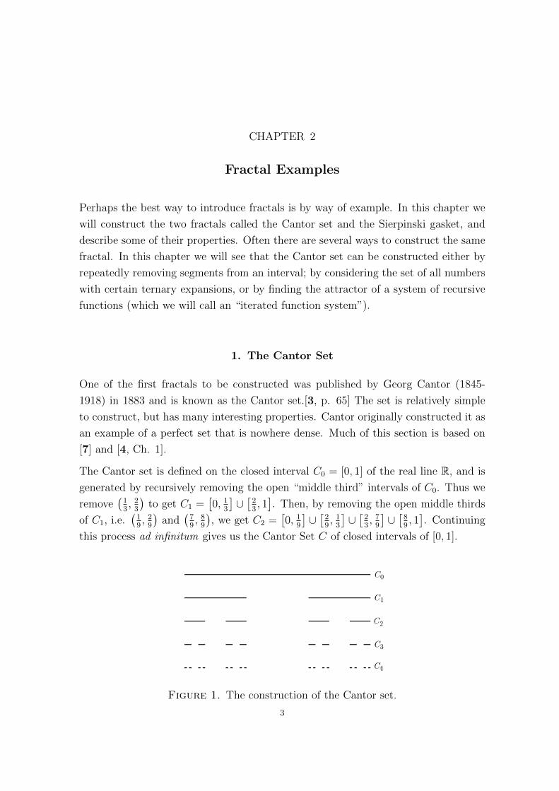
The Cantor set is defined on the closed interval C0 = [0, 1] of the real line R, and is

generated by recursively removing the open “middle third” intervals of C0. Thus we

remove(13, 23

)to get C1 =

[0, 1

3

]∪[23, 1]. Then, by removing the open middle thirds

of C1, i.e.(19, 29

)and

(79, 89

), we get C2 =

[0, 1

9

]∪[29, 13

]∪[23, 79

]∪[89, 1]. Continuing

this process ad infinitum gives us the Cantor Set C of closed intervals of [0, 1].

Figure 1. The construction of the Cantor set.

3

Chapter 2 Page 4

Notice that the sequence C0 ⊇ C1 ⊇ C2 ⊇ · · · ⊇ Cn is decreasing for any n ∈ N, hence

we may formally define the Cantor set to be the limit of the of the intersection of

these sets,

C =∞⋂n=0

Cn.

The Cantor set C is formed by removing a countable number of open intervals from

[0, 1], the union of which is open. The complement of this union is closed, so C is

closed. C is clearly bounded and hence compact by the Heine-Borel theorem.

It is easy to see that Cn consists of 2n intervals of length(13

)n. Thus the total length

of Cn is 2n(13

)n=(23

)n, and hence the total length of the Cantor set C is

limn→∞

(2

3

)n= 0.

This implies that the Cantor set has no intervals.

Observe that each endpoint of Cn is an endpoint of Cn+1, and that, by induction, each

endpoint of Cn is an endpoint of Cm for all m ≥ n. One might expect the Cantor set

to consist only of the endpoints of the sets Cn, but we will see that this is not the

case.

First note that any number x in [0, 1] has a base 3 or ternary representation

x =∞∑j=0

aj3j

with digits aj ∈ {0, 1, 2}.

We shall denote ternary expansions with subscript 3 to distinguish them from decimal

expansions, and refer to a “ternary point” rather than a decimal point. Note that

some numbers can have two representations; for example, 13

= (0.02̄)3 = (0.10̄)3.1

Proposition 2.1. A point x ∈ [0, 1] belongs to the Cantor set C if and only if x has

a ternary expansion with digits aj ∈ {0, 2}.

Proof. This proof is based on [4, p. 4]. All ternary expansions of x have digit 1

at the first place to the right of the ternary point if and only if x is strictly between

(0.10̄)3 = 13

and (0.12̄)3 = 23. If we remove all such x we remove the open interval(

13, 23

)and get C1, thus C1 contains no x whose first ternary digit is 1. Now, for

some x in C1, the second value to the right of the ternary point is 1 if and only if x

1This is not unique to the ternary system; for example, the decimal expansion of 110 is 0.10̄ = 0.09̄.

Chapter 2 Page 5

is in(19, 29

)or(79, 89

). These are the intervals removed from C1 to get C2. Thus C2

has no numbers with a ternary expansion with digit 1 at the first or second place.

Proceeding similarly we can see that for n > 2, Cn has no ternary digits with value 1

at the first n places. Thus C =⋂∞n=0Cn is the set of points x in [0, 1] with a ternary

expansion without ternary digits 1. �

It follows from this result that the Cantor set is uncountable (see [9, p.155] for a full

proof).

Proposition 2.2. The point 14

belongs to C but is not an endpoint of any Cn.

Proof. Dividing 1 = (1)3 by 4 = (11)3 in ternary shows that 14

has ternary

representation (0.02)3, so 14∈ C by Proposition 2.1.

It remains to show that 14

is not an endpoint of any Cn. By the construction of C,

it is clear that all endpoints of Cn are of the form m3k

for m, k non-negative integers.

We show that 14

is not of this form. Suppose (for a contradiction) that it is. Then14

= m3k

, and so 4m = 3k, and clearly 4m is even for all m. But 3k = 3× · · · × 3︸ ︷︷ ︸k−times

, and

since 3 is a prime, this is the unique prime factorisation of 3k. Hence 2 is not a prime

factor of 3k and so 3k is odd for all k, a contradiction. �

We say a set X is perfect if it is precisely the set of limit points of X.

Theorem 2.3. The Cantor set C is a perfect set.

Proof. Any x ∈ C has a ternary expansion

x =∞∑j=1

aj3j,

for aj ∈ {0, 2}. The representation of x up to k digits is given by

xk =k∑j=1

aj3j,

which is in Ck. Now, to prove the theorem, we show that as k tends to infinity, xk

tends to the point x in C. We have

|x− xk| =∞∑

j=k+1

aj3j≤

∞∑j=k+1

2

3j=

1

3k.

Now limk→∞13k

= 0, so by the squeezing rule, limk→∞ |x−xk| = 0, and so limk→∞ xk =

x, as required. �

Chapter 2 Page 6

A set X being perfect is equivalent to X being closed with no isolated points.

The Cantor set is totally disconnected space of total length (or Lebesgue measure)

0, so it is a collection of isolated points, each of which has (topological) dimension 0

(see Chapter 3). In this sense, one might expect the Cantor set to have dimension 0

(we see later that 0 is its topological dimension), but this value of dimension does not

seem to do the set justice, since the Cantor set is uncountable, and it has the same

cardinality of the 1-dimensional interval [0,1]. Thus a value between 0 and 1 seems

appropriate. We see later that the Cantor set has Hausdorff dimension log 2log 3≈ 0.6309.

2. The Cantor Set as an Iterated Function System

A useful way to define a “self-similar” set such as the Cantor set is as the attractor of

an iterated function system (IFS) of contraction mappings. We define these

notions now.

Let X, Y be metric spaces and d be the Euclidean metric. Let λ > 0. We define a

similarity with scale factor λ to be a function f : X → Y such that d(f(a), f(b)) =

λd(a, b), for all a, b ∈ X.

In particular, f is a contraction mapping if it maps from X to itself and λ < 1.

An iterated function system on a complete metric space X is a set of contraction

mappings {fi : X → X : i = 1, 2, . . . , k}, for k ∈ N, with scale factors {λi : i =

1, 2, . . . , k}.

We say a non-empty compact set A ⊆ X is an attractor of the above IFS if A =

f1(A) ∪ f2(A) ∪ · · · ∪ fk(A).

For x ∈ [0, 1], the Cantor set can be generated by the following IFS:

f1(x) =1

3x;

f2(x) =1

3x+

2

3.

We know C0 = [0, 1], so C1 = f1(C0) ∪ f2(C0), and so C2 = f1(C1) ∪ f2(C1). So by

induction,

Cn = f1(Cn−1) ∪ f2(Cn−1). (2.1)

The following proposition says what happens when we take the infinite intersection

or “limit”. We show that C is the attractor of the IFS above.

Chapter 2 Page 7

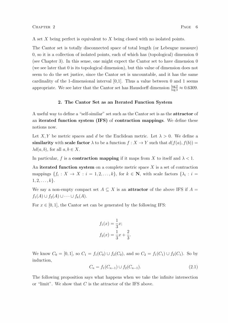
Proposition 2.4.

C = f1(C) ∪ f2(C).

Proof. Note that Equation (2.1) can be written as Cn+1 = f1(Cn) ∪ f2(Cn).

Firstly, we want to show that C ⊆ f1(C) ∪ f2(C). Suppose that x ∈ C. Then

x ∈ C1, and thus x ∈[0, 1

3

]or x ∈

[23, 1]. Consider the case x ∈

[23, 1]. Then for

any n, we know that x ∈ Cn+1 = f1(Cn) ∪ f2(Cn). But f1(Cn) ⊆ f1([0, 1]) =[0, 1

3

],

so x /∈ f1(Cn). Thus x ∈ f2(Cn) = Cn+23

, and 3x − 2 ∈ Cn (for all n). Thus

3x − 2 ∈⋂∞n=0Cn = C, and so x ∈ C+2

3= f2(C). Proceeding similarly for the case

x ∈[0, 1

3

]shows that x ∈ f1(C). Thus x ∈ C implies thatx ∈ f1(C) ∪ f2(C).

The second relationship to prove is C ⊇ f1(C) ∪ f2(C). Suppose that x ∈ f1(C) ∪f2(C). Then x ∈ f1(C) or x ∈ f2(C). Consider the case x ∈ f2(C) = C+2

3. Then

3x − 2 ∈ C, so 3x − 2 ∈ Cn for all n. Thus x ∈ Cn+23

= f2(Cn) ⊆ Cn=1. Thus x ∈⋂∞n=0Cn+1 =

⋂∞n=0Cn = C. The case x ∈ f1(C) is similar. Thus x ∈ f1(C) ∪ f2(C)

implies that x ∈ C, and we have proved the proposition. �

3. Sierpinski Gasket

Here is another standard fractal. Consider, in the plane R2, the area enclosed by

the equilateral triangle S0 with sides of length 1. Now S0 can be split into 4 similar

equilateral triangles, with sides of length 12

(see Figure 3), by drawing a straight line

between each midpoint of the sides of S0. We remove the interior of the middle such

triangle, and call the area enclosed by the remaining 3 triangles S1. Splitting the 3

triangles of S1 up and again removing the interior of the “middle fourth” triangle gives

us S2. Continuing, ad infinitum, the process of removing “middle fourth” triangles

constructs the Sierpinski Gasket S.

We have S0 ⊇ S1 ⊇ S2 ⊇ · · · ⊇ Sn. Then the Sierpinski Gasket is

S =∞⋂n=0

Sn.

Sn clearly consists of 3n triangles with sides of length 12n

. Note that half the length

of one side is 12n+1 , so the height of each triangle in Sn is√(

1

2n

)2

−(

1

2n+1

)2

=

√1

2sn− 1

22n+2=

√3

22n+2=

√3

2n+1,

Chapter 2 Page 8

Figure 2. The construction of the Sierpinski Gasket.

and thus the area of each triangle in Sn is(1

2

)(1

2n+1

)( √3

2n+1

)=

√3

22n+3,

and so the area of S is

limn→∞

√3

22n+3= 0.

Each triangle in Sn has perimeter 3(

12n

)= 3

2n, and since the sides of each triangle do

not overlap, the total length of S is

limn→∞

3n(

3

2n

)= lim

n→∞3

(3

2

)n=∞.

As we have just seen, the Sierpinski Gasket has no area, and so it would make little

sense to talk of it being a two-dimensional object. In the sense that it has no area, it

is like the one-dimensional line, but unlike the line, it has infinite length in a bounded

region, so in this way it is “bigger” than the one-dimensional line. If one were to allow

for non-integer dimension, then one would guess the dimension of S to be between 1

and 2. We shall see later that S has fractal dimension log 3log 2≈ 1.5849.

CHAPTER 3

Non-Fractal Dimension

1. Euclidean Dimension

The Euclidean dimension dimE of a set is simply the number of co-ordinates re-

quired to describe each point in that set.[5, p. 11] It follows that dimE is always an

integer and that any set defined in the Euclidean space En (or Rn) has dimE = n. This

notion of dimension makes sense for describing a space as a whole, but is less accurate

for describing sets in that space. For example, both a cube and an isolated point in

E3 have Euclidean dimension 3. Also it does not adequately describe a shape such as

(the boundary of) a circle in R2. In one sense, the circle is 2-dimensional since the

points in the set are occupying 2-dimensions, but the circle itself is “a length without

breadth”, which makes one think of it as being a one-dimensional object. This latter

notion of dimension is what we will define later as topological dimension.

Example 3.1. Trivially, dimE Rn = n.

The Cantor set C has dimE C = 1, since it is defined in R.

The Seirpinksi Gasket S has dimE S = 2, since it defined in R2. �

2. Topological Dimension

If we consider “length”, “breadth”, and “depth” to be the 3 dimensions of R3, then

we can see that the intuition for topological dimension goes back to Euclid, who says

that “a point is that of which there is no part”; “a line is a length without breadth”;

“a surface is that which has length and breadth only”, and “a solid is a (figure)

having length, breadth and depth”.[8] It was not, however, until the 20th century

that a formal definition of topological dimension was arrived at.

Unlike Euclidean dimension, Topological dimension aims to define the dimension of

a set in a way that is irrespective of the dimension of the space that the set is defined

in. Naturally, any sensible definition of the topological dimension of a set will not

allow the dimension of a set to be greater than the dimension of the space it is defined

in. Also, it will not allow for topologically equivalent (homeomorphic) sets to have

different dimensions. The two most important definitions of topological dimension

9

Chapter 3 Page 10

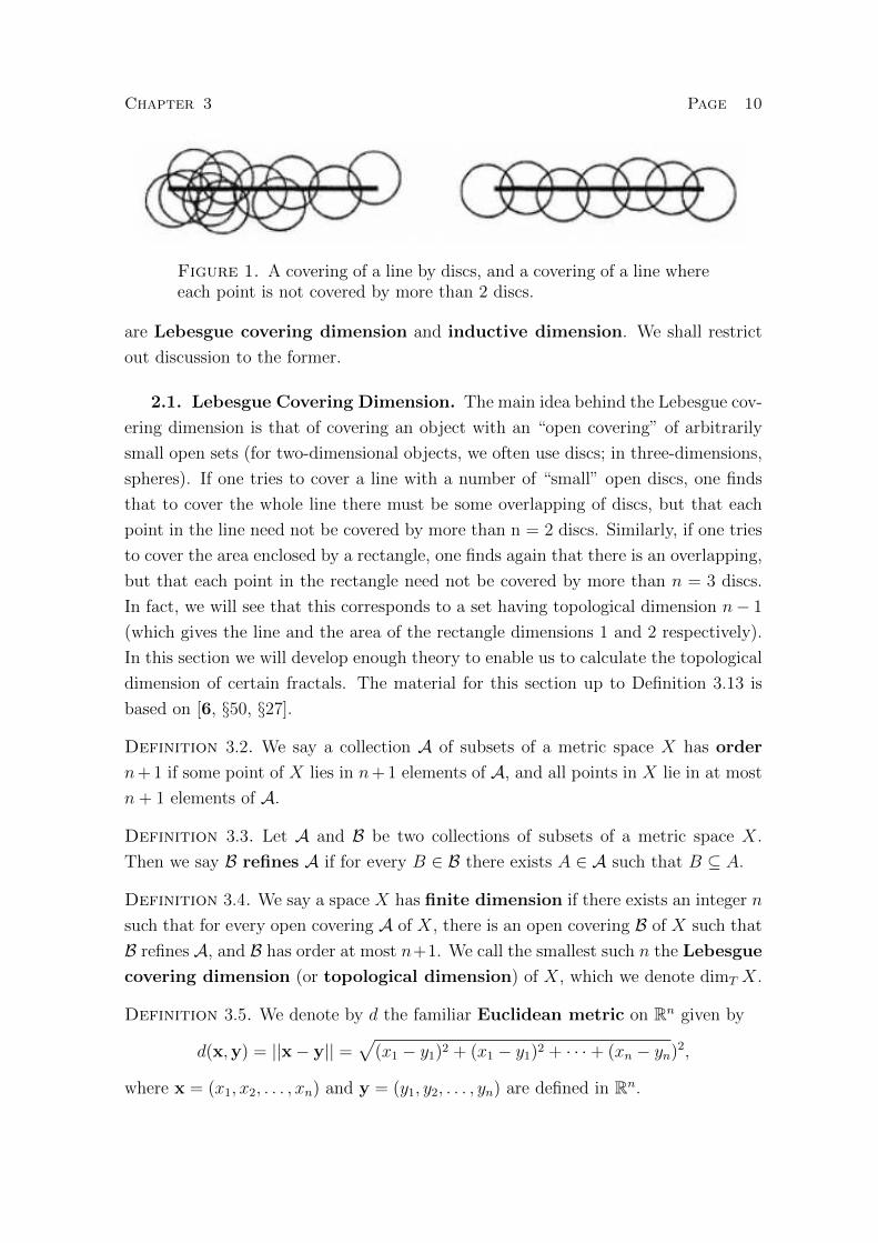
Figure 1. A covering of a line by discs, and a covering of a line whereeach point is not covered by more than 2 discs.

are Lebesgue covering dimension and inductive dimension. We shall restrict

out discussion to the former.

2.1. Lebesgue Covering Dimension. The main idea behind the Lebesgue cov-

ering dimension is that of covering an object with an “open covering” of arbitrarily

small open sets (for two-dimensional objects, we often use discs; in three-dimensions,

spheres). If one tries to cover a line with a number of “small” open discs, one finds

that to cover the whole line there must be some overlapping of discs, but that each

point in the line need not be covered by more than n = 2 discs. Similarly, if one tries

to cover the area enclosed by a rectangle, one finds again that there is an overlapping,

but that each point in the rectangle need not be covered by more than n = 3 discs.

In fact, we will see that this corresponds to a set having topological dimension n− 1

(which gives the line and the area of the rectangle dimensions 1 and 2 respectively).

In this section we will develop enough theory to enable us to calculate the topological

dimension of certain fractals. The material for this section up to Definition 3.13 is

based on [6, §50, §27].

Definition 3.2. We say a collection A of subsets of a metric space X has order

n+ 1 if some point of X lies in n+ 1 elements of A, and all points in X lie in at most

n+ 1 elements of A.

Definition 3.3. Let A and B be two collections of subsets of a metric space X.

Then we say B refines A if for every B ∈ B there exists A ∈ A such that B ⊆ A.

Definition 3.4. We say a space X has finite dimension if there exists an integer n

such that for every open covering A of X, there is an open covering B of X such that

B refines A, and B has order at most n+1. We call the smallest such n the Lebesgue

covering dimension (or topological dimension) of X, which we denote dimT X.

Definition 3.5. We denote by d the familiar Euclidean metric on Rn given by

d(x,y) = ||x− y|| =√

(x1 − y1)2 + (x1 − y1)2 + · · ·+ (xn − yn)2,

where x = (x1, x2, . . . , xn) and y = (y1, y2, . . . , yn) are defined in Rn.

Chapter 3 Page 11

Definition 3.6. Let (X, d) be a metric space, and let A be a nonempty subset of X.

Then for x ∈ X we define the distance between x and A to be

d(x, A) = inf{d(x, a) : a ∈ A}.

Lemma 3.7. Let A be a subset of X, and set g(x) = d(x, A). Then g is continuous.

Proof. Let x,y ∈ X. Then for each a ∈ A we have (by the triangle inequality)

d(x, A) ≤ d(x, a) ≤ d(x,y) + d(y, a),

and so

d(x, A)− d(x,y) ≤ d(y, a) = inf d(y, a) = d(y, A).

Thus

d(x, A)− d(y, A) ≤ d(x,y).

A similar argument gives

d(y, A)− d(x, A) ≤ d(x,y).

This implies that g(x) is continuous. �

The following lemma is known as Lebesgue’s number lemma, and is useful for

finding a refinement of an open covering of a compact metric space.

Lemma 3.8. Let A be an open covering of the metric space (X, d), where X is compact.

Then there exists a δ > 0 such that for every subset B ⊆ X with diameter less than

δ, there is an A ∈ A such that B ⊆ A. We call δ a Lebesgue number of the

covering A.

Proof. In the case where X = A, for some element A ∈ A, we have that every

subset of X is contained in A, hence any δ > 0 is a Lebesgue number for A.

In the case where X is not an element of some A ∈ A, consider the finite subcover

{A1, . . . , An} ⊆ A of X, which exists by the compactness of X.

Set Ci = X − Ai, and define f : X → R by

f(x) =1

n

n∑i=1

d(x,Ci).

That is, for each x ∈ X, f(x) takes the value of the average of the minimum distances

between x and each Ci.

Chapter 3 Page 12

We show that f(x) > 0 for all x ∈ X. For some x ∈ X, choose i such that x ∈ Ai.Now choose ε > 0 such that Bε(x) ⊆ Ai. (We know that such an ε exists since Ai is

open). Now we have d(x,Ci) ≥ ε (by the definition of Ci), and so f(x) ≥ εn. Now

by Lemma 3.7 is is clear that f is continuous, and we know that f is greater than 0,

hence f has a minimum value δ. Let S be a subset of X, with diameter < ε. Then

there exists some x0 ∈ S such that Bδ(x0) ⊇ S. Now choose m such that d(x0, Cm)

is the largest of all the numbers d(x0, Ci). Then

δ ≤ f(x0) ≤ d(x0, Cm).

Thus Bδ(x0) ⊆ Am, and since S ⊆ Bδ(x0) we have S ⊆ Am, and so δ is a Lebesgue

number for X. �

Theorem 3.9. Let X be a compact subspace of R. Then dimT X ≤ 1.

Proof. We shall show that there exists an open covering B of X with order 2

that refines every open covering A of X, thus proving the theorem.

Define B1 to be the collection of all open intervals in R of the form (k, k+1), for k some

integer. Let B2 be the collection of all open intervals in R of the form (k − 12, k + 1

2),

for k an integer. Then B = B1 ∪B2 is an open covering of R. Note that all sets in B1and B2 have diameter 1, and are disjoint. Thus a point in B can be in at most one

set of B1 and one set of B2, hence the open covering B has order 2.

Now let X be a compact subspace of R. Consider an open covering C of X. Then this

covering has a Lebesgue number δ > 0. This means that any collection of subsets of

X with diameter less than δ is a refinement of C. Now consider the map f : R → Rgiven by f(x) = 1

2δx, where the domain is the set of all elements x in A. Then the

image of f provides an open covering, call it D, of order 2 with each element in Dhaving diameter 1

2δ, which is less than δ, as required. The intersection of D with X

provides a covering that refines C and has order 2. �

Example 3.10. The interval [0, 1] has dimT = 1.

Let X = [0, 1]. Then by Theorem 3.9, dimT X ≤ 1. Now let A be a covering of X

by the intervals [0, 1) and (0, 1]. Then A has order 2. Note that any arbitrary open

covering of X must be a refinement of A. We show that if B is an open covering of

X that refines A, then it has order at least 2.

Let U be an element of B and let V be the union of the other elements in B. Suppose

that B has order 1. Then, by definition, no point in X lies in more than 1 element of

B. This implies that U and V do not overlap and are disjoint. But then B is not a

covering of X, a contradiction. Thus B has order at least 2, and so dimT X ≥ 1. �

Chapter 3 Page 13

Theorem 3.11. Let X be a finite dimensional space, and let Y be a closed subspace

of X. Then Y is finite dimensional and dimT Y ≤ dimT X.

Proof. Let dimX = n and let A be a collection of sets open in Y that covers Y

(i.e. an arbitrary open covering of Y ). For each A ∈ A, choose an open set A′ in X

such that A′ ∩ Y = A. Now consider a covering B of X composed of each A′ set and

the (open) set X − Y . Since dimT X = n, by definition there is an open covering Cof X that refines B and has order at most n + 1. Then {C ∩ Y : C ∈ C} provides a

covering of Y of open sets in Y that refines A and has order at most n+ 1. Hence Y

has finite dimension, and dimension at most n. �

Definition 3.12. From [4, p. 41]. Let A be a subset of a metric space (X, d), where

d is the Euclidean metric. Then we say that the diameter of A is

diam A = sup{d(x,y) : x,y ∈ A}

Definition 3.13. If A is a covering of the metric space (X, d) then the mesh of Ais the supremum of the diameters of of all elements A ∈ A.

Theorem 3.14. Let X be a compact space. Then dimT X ≤ n if and only if for every

ε > 0 there exists an open cover of X with order ≤ n and mesh ≤ ε

Proof. Proof based on [4, p. 98]. Suppose dimT X ≤ n, and let ε > 0. Then the

collection A of all open subsets of diameter ≤ ε is a covering of X. Since dimT X ≤ n,

by definition there is a refinement B of A of order at most n. Since B is a refinement

of A, clearly mesh B ≤ mesh A = ε.

To prove the other direction, suppose that for every ε > 0 there exists an open cover

of X with order ≤ n and mesh ≤ ε. Let A be an arbitrary open cover of X. Then,

by Lemma 3.8, A has a positive Lebesgue number δ. Let B be an open cover of X

with order at most n and mesh smaller than both δ and ε. Then by Lemma 3.8, B is

a refinement of A. Hence dimT X ≤ n. �

Example 3.15. The Cantor set C has dimT C = 0.

Recall that for an any n, Cn is made up of 2n intervals of length 13n

. Note that any two

of these intervals are apart by a distance of at least 13n

. Now let r > 0 be a number

such that r is strictly less than 12· 13n

. Then the collection A of r−neighbourhoods of

each of the 2n intervals of Cn forms an open covering of Cn with order 1 and mesh at

most 13n

+ 2r.

Chapter 3 Page 14

Now for any ε > 0 we can choose n large enough such that 13n

+ 2r ≤ ε, and we have

that A is a covering of Cn (and C) with order 1 and mesh ≤ ε. Thus by Theorem

3.14 we have dimT S ≤ 0. �

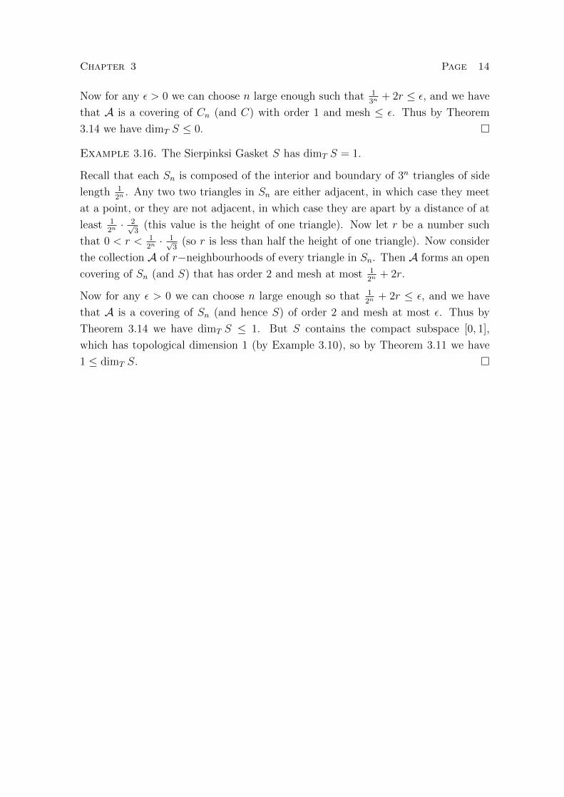
Example 3.16. The Sierpinksi Gasket S has dimT S = 1.

Recall that each Sn is composed of the interior and boundary of 3n triangles of side

length 12n

. Any two two triangles in Sn are either adjacent, in which case they meet

at a point, or they are not adjacent, in which case they are apart by a distance of at

least 12n· 2√

3(this value is the height of one triangle). Now let r be a number such

that 0 < r < 12n· 1√

3(so r is less than half the height of one triangle). Now consider

the collection A of r−neighbourhoods of every triangle in Sn. Then A forms an open

covering of Sn (and S) that has order 2 and mesh at most 12n

+ 2r.

Now for any ε > 0 we can choose n large enough so that 12n

+ 2r ≤ ε, and we have

that A is a covering of Sn (and hence S) of order 2 and mesh at most ε. Thus by

Theorem 3.14 we have dimT S ≤ 1. But S contains the compact subspace [0, 1],

which has topological dimension 1 (by Example 3.10), so by Theorem 3.11 we have

1 ≤ dimT S. �

CHAPTER 4

Fractal Dimension

We discussed briefly, in chapter one, why one might expect the dimension of some

sets, such as the Cantor set and Sierpinksi Gasket, to take a non-integer value. It was

supposed that the dimension of the Cantor Set should be between 0 and 1. We have

seen in the previous chapter that 0 and 1 are the values of the Cantor set’s topological

and Euclidean dimension respectively. In this section we allow for the Cantor Set to

take a dimensional value strictly between 0 and 1. In general, we call a dimension

that can take a non-integer value a fractal dimension. Mathematicians have come

up with many fractal dimensions, each with advantages and disadvantages. Perhaps

the most important one is the one that Mandelbrot singled out in his definition of a

“fractal”, namely the Hausdorff dimension (or Hausdorff Besicovitch dimen-

sion). Other useful fractal dimensions, which we shall discuss in this chapter, are the

similarity dimension, lower box-counting dimension, upper box-counting

dimension, and box-counting dimension. For many sets, the values of these di-

mensions coincide, and one may talk loosely of the fractal dimension of the set.

Note that any set of non-integer Hausdorff dimension is certainly a fractal, by Man-

delbrot’s definition, since topological dimension is always an integer. The following

section is based on [10].

1. The Hausdorff Dimension

If U is a non-empty subset of Rn then the diameter of U is the greatest distance

between any two points in U , i.e. |U | = sup {|x− y| : x, y ∈ U}. We define a δ-cover

of a set X to be a countable collection of sets {Ui} of diameter at most δ such that

X ⊂⋃∞i=1 for all i. Now consider the sum of the s-th powers of each |Ui|. The

minimal such cover of X, for a given δ > 0, is defined as the Hausdorff content

of X

Hsδ(X) = inf

{∞∑i=1

|Ui|s : Ui is a δ-cover of X

}.

The limit as δ → 0 is the Hausdorff measure

Hs(X) = limδ→0Hsδ(X).

15

Chapter 4 Page 16

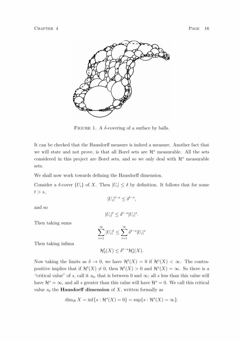
Figure 1. A δ-covering of a surface by balls.

It can be checked that the Hausdorff measure is indeed a measure. Another fact that

we will state and not prove, is that all Borel sets are Hs measurable. All the sets

considered in this project are Borel sets, and so we only deal with Hs measurable

sets.

We shall now work towards defining the Hausdorff dimension.

Consider a δ-cover {Ui} of X. Then |Ui| ≤ δ by definition. It follows that for some

t > s,

|Ui|t−s ≤ δt−s,

and so

|Ui|t ≤ δt−s|Ui|s.

Then taking sums∞∑i=1

|Ui|t ≤∞∑i=1

δt−s|Ui|s

Then taking infima

Htδ(X) ≤ δt−sHs

δ(X).

Now taking the limits as δ → 0, we have Ht(X) = 0 if Hs(X) < ∞. The contra-

positive implies that if Ht(X) 6= 0, then Ht(X) > 0 and Hs(X) = ∞. So there is a

“critical value” of s, call it s0, that is between 0 and ∞; all s less than this value will

have Hs =∞, and all s greater than this value will have Hs = 0. We call this critical

value s0 the Hausdorff dimension of X, written formally as

dimH X = inf{s : Hs(X) = 0} = sup{s : Hs(X) =∞}.

Chapter 4 Page 17

We shall now state and prove two fundamental properties of Hausdorff dimension.

Theorem 4.1. Let A and B be Borel sets. If A ⊆ B, then dimA ≤ dimB.

Proof. From [4, p. 168]. A ⊆ B implies that Hs(A) ≤ Hs(B) for all s (by a

property of measures). Thus sup{s : Hs(A) = ∞} ≤ sup{s : Hs(B) = ∞}; that is,

dimA ≤ dimB. �

Theorem 4.2. Let X ⊆ Rn, and λ > 0. Then

Hs(λX) = λsHs(X).

Proof. We write∑

as shorthand for∑∞

i=1. Let {Ui} be a δ-cover of X. Then

{λUi} is a λδ-cover of λX. Hence

Hsλδ(λX) ≤

∑|λUi|s = λs

∑|Ui|s ≤ λsHs

δ(X).

As δ → 0, we have Hs(λX) ≤ λsHs(X). To prove the inequality holds the other way,

we proceed similarly. Let {Ui} be a δ-cover of λX. Then {λ−1Ui} is a λ−1δ-cover of

X. Thus

Hsλ−1δ(X) ≤

∑|λ−1Ui|

s= λ−s

∑|Ui|s ≤ λ−sHs

λ−1δ(λX).

So as δ → 0, we have λsHs(X) ≤ Hs(λX) as required. �

Example 4.3. We will show that the Cantor set C has dimH C = log 2log 3≈ 0.6309.

We will first “guess” the value of s for the dimension of the Cantor set C, and then

prove dimH C = s.

The Cantor set C can be split into a two parts, CL = C ∩ [0, 13], and CR = C ∩ [2

3, 1].

These are similarities of C with scaling factor 13. Now C is the disjoint union CL∪CR,

so by a basic property of measures, and then by Proposition (4.2), we have, for any s

Hs(C) = Hs(CL) ∪Hs(CR) =

(1

3

)sHs(C) +

(1

3

)sHs(C).

Then if Hs(C) is finite and non-zero at the critical value (we will prove it is soon),

we can divide by Hs(C) to get 1 =(13

)s+(13

)s. Solving for s, first note that(

1

3

)s=

(1

2

). (1.1)

Then taking logs we see that s log(13

)= log

(12

), and so s =

log( 12)

log( 13)

= log 2log 3≈ 0.6309.

Now that we have “guessed” the critical value of s, we must show that 0 < Hs(C) <∞for s = log 2

log 3. This will imply that dimH C = s.

Chapter 4 Page 18

Consider a covering {Ui} of C. Recall that C consists of 2n intervals of length 13n

.

Then for a minimum covering of C, we have sum consisting of 2n sets of diameter

| 13n|. Hence for s = log 2

log 3(and writing

∑as shorthand for

∑∞i=1) we have

Hs3−n(C) ≤

∑|Ui|s = 2n3−ns = 2

(1

3

)s= 2

(1

2

)= 1.

Letting n→∞, we get Hs(C) ≤ 1 <∞.

It now remains to show that Hs(C) > 0. We will show that Hs(C) ≥ 12

=(13

)s. For

each Ui, we have some n such that

1

3n+1≤ |Ui| <

1

3n(1.2)

Then Ui can intersect at most one interval of Cn, since the “gaps” between intervals

of Cn are of length 13n

. If m ≥ n, the number of intervals of Cm that Ui intersects is

at most 2m−n = 2m3−sn ≤ 2m3s|Ui|s. (The first equality is by (1.1). To see the last

inequality, observe that 13n≤ 3|Ui| by (1.2), then take powers).

If we choose m such that 13m+1 ≤ |Ui| for all Ui, then the set {Ui} will intersect all 2m

intervals of length 13m

. Hence, counting each interval, we get

2m ≤∑

2m3s|Ui|s

So 1 ≤∑

3s|Ui|s, hence 3−s ≤∑|Ui|s, as required. �

2. Similarity Dimension

In this section we will define similarity dimension, which is an easy to calculate

dimension, but is unfortunately only applicable to a relatively small number of sets,

and not all fractals. In fact we will see later that it gives an exact estimate of Hausdorff

dimension for self-similar for which Moran’s open set condition holds (defined later).

When dealing with self-similar sets, similarity dimension has the advantages of being

somewhat more intuitive and easier to deal with than the Hausdorff dimension. Before

we give the definition, we give the following motivation for it, based on Mandelbrot’s

exposition in [1, p. 37].

Start by considering the one dimensional Euclidean space E (or just the real line R).

It is clear that any interval [0, a) on this line can be partitioned into a number N = b

Chapter 4 Page 19

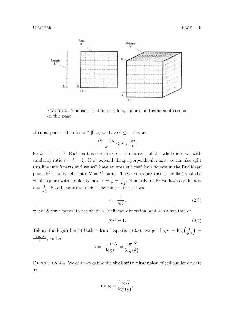
Figure 2. The construction of a line, square, and cube as describedon this page.

of equal parts. Then for x ∈ [0, a) we have 0 ≤ x < a, or

(k − 1)a

b≤ x <

ka

b,

for k = 1, . . . , b. Each part is a scaling, or “similarity”, of the whole interval with

similarity ratio r = 1b

= 1N

. If we expand along a perpendicular axis, we can also split

this line into b parts and we will have an area enclosed by a square in the Euclidean

plane E2 that is split into N = b2 parts. These parts are then a similarity of the

whole square with similarity ratio r = 1b

= 1

N12

. Similarly, in E3 we have a cube and

r = 1

N13

. So all shapes we define like this are of the form

r =1

N1s

, (2.3)

where S corresponds to the shape’s Euclidean dimension, and s is a solution of

Nrs = 1. (2.4)

Taking the logarithm of both sides of equation (2.3), we get log r = log(

1

N1s

)=

−(logN)s

, and so

s =− logN

log r=

logN

log(1r

) .Definition 4.4. We can now define the similarity dimension of self-similar objects

as

dimS =logN

log(1r

) ,

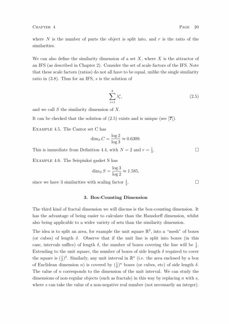
Chapter 4 Page 20

where N is the number of parts the object is split into, and r is the ratio of the

similarities.

We can also define the similarity dimension of a set X, where X is the attractor of

an IFS (as described in Chapter 2). Consider the set of scale factors of the IFS. Note

that these scale factors (ratios) do not all have to be equal, unlike the single similarity

ratio in (3.8). Thus for an IFS, s is the solution of

k∑i=1

λsi , (2.5)

and we call S the similarity dimension of X.

It can be checked that the solution of (2.5) exists and is unique (see [7]).

Example 4.5. The Cantor set C has

dimS C =log 2

log 3≈ 0.6309.

This is immediate from Definition 4.4, with N = 2 and r = 13. �

Example 4.6. The Seirpinksi gasket S has

dimS S =log 3

log 2≈ 1.585,

since we have 3 similarities with scaling factor 12. �

3. Box-Counting Dimension

The third kind of fractal dimension we will discuss is the box-counting dimension. It

has the advantage of being easier to calculate than the Hausdorff dimension, whilst

also being applicable to a wider variety of sets than the similarity dimension.

The idea is to split an area, for example the unit square R2, into a “mesh” of boxes

(or cubes) of length δ. Observe that if the unit line is split into boxes (in this

case, intervals suffice) of length δ, the number of boxes covering the line will be 1δ.

Extending to the unit square, the number of boxes of side length δ required to cover

the square is (1δ)2. Similarly, any unit interval in Rn (i.e. the area enclosed by a box

of Euclidean dimension n) is covered by (1δ)n boxes (or cubes, etc) of side length δ.

The value of n corresponds to the dimension of the unit interval. We can study the

dimensions of non-regular objects (such as fractals) in this way by replacing n with s,

where s can take the value of a non-negative real number (not necessarily an integer).

Chapter 4 Page 21

If we split the plane into a mesh of boxes of length δ, then any set X in the plane

can be completely covered by a number of boxes, we call the minimum such number

N . The value of N clearly depends on the the size of the boxes. Notice that as δ

decreases, the number of boxes required to cover X increases. We write Nδ(X) for

the minimum number of boxes of length δ required to completely cover

X. As we have seen above, we can expect an object to be covered by Nδ(X) = (1δ)s

boxes, where s corresponds to the dimension of the object. Solving for s, we take logs

of both sides to get

s =logNδ(X)

log 1δ

=logNδ(X)

− log δ.

We are interested in what happens as δ becomes arbitrarily small, so we define the

box-counting dimension of a set X in Rn to be

dimBX = limδ→0

logNδ(X)

− log δ,

where Nδ(X) is the smallest number of sets of diameter not exceeding δ, required

to cover X. In general, this limit may not exist, in which case the box-counting

dimension is not defined. However, the limit exists if (and only if) the upper limit

and lower limit are equal, then the (ordinary) limit takes the same value as the upper

and lower limit. We define then, the lower box-counting dimension dimBX and

upper box-counting dimension dimBX respectively by

dimBX = lim infδ→0

logNδ(X)

− log δ,

dimBX = lim supδ→0

logNδ(X)

− log δ.

Note the general inequality dimBX ≤ dimBX ≤ dimBX. So if dimBX = dimBX,

then dimBX = dimBX = dimBX.

Note that by the above construction it’s clear that dimBX ≤ dimE X, since X is

simply the amount of co-ordinates of the space that X is defined in.

We can take the limit as δ tends to 0 directly, or through a decreasing sequence like

in the following lemma.

Chapter 4 Page 22

Lemma 4.7. Let X be a subset of Rn, and let δn be a decreasing sequence such that

c ≤ δn+1

δn, for some 0 < c < 1, and cn = δk . Then

dimBX = limn→∞

logNδn(X)

− log δn.

Proof. If δn+1 ≤ δ < δn then

logNδ(X)

− log δ≤

logNδn+1(X)

− log δn≤

logNδn+1(X)

− log δn+1 + log(δn+1/δn)≤

logNδn+1(X)

− log δn+1 + log c.

Taking upper limits we have,

lim supδ→0

logNδ(X)

− log δ≤ lim sup

n→∞

logNδn(X)

− log δn.

Also, taking lower limits, we have

lim infδ→0

logNδ(X)

− log δ≤ lim sup

n→∞

logNδn(X)

− log δn.

A similar argument shows that the opposite inequalities hold. �

Example 4.8. The Cantor set C has dimB C = log 2log 3≈ 0.6309

For any Cn, we require a covering of the 2n intervals of length 13n

. Consider δ > 0

such that1

3n< δ ≤ 1

3n−1.

Then it takes at most 2n intervals of length δ to cover Cn (and C), so we have

Nδ(C) ≤ 2n. Thus (making use of Lemma 4.7), we have

dimBC = lim supδ→0

logNδ(C)

− log δ= lim sup

n→∞

logNδn(C)

− log δn≤ lim sup

n→∞

log 2n

log 3n−1=

log 2

log 3.

To prove the opposite inequality, consider intervals of length δ where

1

3n+1≤ δ <

1

3n.

Then each interval intersects at most one of the 2n intervals of length 13n

of Cn. Thus

at least 2n intervals of length δ are needed to cover Cn (and C), so Nδ(C) ≥ 2n.

Proceeding as before and taking lower limits gives dimBC ≥ log 2log 3

as required. �

The box-counting dimension has some undesirable properties. One is that box-

counting dimension is not countably stable. Note that any singleton point has box-

counting dimension 0 (as one would expect), since it takes only 1 box of of side length

δ to cover a point, and limδ→0log 1− log δ

= 0. However, a countable collection of points

does not necessarily have box-counting dimension 0. We shall illustrate this with an

example.

Chapter 4 Page 23

Example 4.9. Let S be the closure of the set of all points of the form 1n, for all

positive integers n; that is, S = {0, 1, 12, 13, . . . }. We show that dimB S = 1

2.

We want to consider coverings of S by sets of arbitrarily small diameter. So let

0 < δ < 12, and let n be the integer such that

1

n(n+ 1)≤ δ <

1

n(n− 1)(3.6)

Let U be an interval such that |U | ≤ δ. Then

|U | ≤ δ <1

n(n− 1)=

1

(n− 1)− 1

n.

So |U | is less than the distance between the n-th point and the (n − 1)-th point in

the set, and so it takes at least n sets of diameter δ to cover S. Thus Nδ(S) ≥ n,

and hence logNδ(S) ≥ log n. Taking logs of the (non-strict) inequality in (3.6) gives

− log δ ≥ log n(n+ 1). Taking quotients of these last two inequalities gives

Nδ(S)

− log δ≥ log n

log n(n+ 1). (3.7)

It is clear by (3.6) that as δ → 0, n → ∞. Thus by letting δ → 0 in (3.7), and then

applying l’Hopital’s rule twice, we get

dimBS ≥ limn→∞

log n

log n(n+ 1)= lim

n→∞

n+ 1

2n+ 1= lim

n→∞

1

2=

1

2.

Now exploiting the other side of (3.6),

δ ≥ 1

n(n+ 1)=

1

n− 1

n+ 1,

so it takes (k + 1) intervals of length δ to cover [0, 1n], in particular, 2 intervals of

length δ to cover [0, 1], so Nδ(S) ≤ 2n. Taking logs of this, and dividing by the logs

of (3.6), we get

Nδ(S)

− log δ≤ log 2n

log n(n− 1). (3.8)

Thus as δ → 0, we get

dimBS ≤ limn→∞

log 2n

log n(n− 1)= lim

n→∞

n− 1

(2n− 1)= lim

n→∞

1

2=

1

2.

Hence dimB S = dimBS = dimBS = 12. �

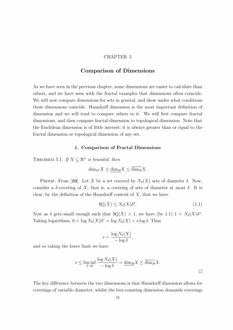
CHAPTER 5

Comparison of Dimensions

As we have seen in the previous chapter, some dimensions are easier to calculate than

others, and we have seen with the fractal examples that dimensions often coincide.

We will now compare dimensions for sets in general, and show under what conditions

these dimensions coincide. Hausdorff dimension is the most important definition of

dimension and we will tend to compare others to it. We will first compare fractal

dimensions, and then compare fractal dimension to topological dimension. Note that

the Euclidean dimension is of little interest; it is always greater than or equal to the

fractal dimension or topological dimension of any set.

1. Comparison of Fractal Dimensions

Theorem 5.1. If X ⊆ Rn is bounded, then

dimH X ≤ dimBX ≤ dimBX.

Proof. From [10]. Let X be a set covered by Nδ(X) sets of diameter δ. Now,

consider a δ-covering of X; that is, a covering of sets of diameter at most δ. It is

clear, by the definition of the Hausdorff content of X, that we have

Hsδ(X) ≤ Nδ(X)δs. (1.1)

Now as δ gets small enough such that Hsδ(X) > 1, we have (by 1.1) 1 < Nδ(X)δs.

Taking logarithms, 0 < logNδ(X)δs = logNδ(X) + s log δ. Thus

s <logNδ(X)

− log δ,

and so taking the lower limit we have

s ≤ lim infδ→0

logNδ(X)

− log δ= dimBX ≤ dimBX.

�

The key difference between the two dimensions is that Hausdorff dimension allows for

coverings of variable diameter, whilst the box-counting dimension demands coverings

24

Chapter 5 Page 25

be of same diameter. We have seen, with the Cantor set and Sierpinski gasket, an

example where the upper box-counting dimension is equal to the Hausdorff dimension.

Now, we say that an IFS satisfies Moran’s open set condition if and only if there

exists a nonempty open set U such that fi(U) ∩ fj(U) = for all i not equal to j and

U ⊇ fi(U). Then a theorem says that if a set X is satisfied, then dimS X = dimH X

(for a proof, see [4, p. 191]).

It’s easy to check (without using the theorem) that the Cantor set and Sierpinski

gasket satisfy Moran’s open set condition.

2. Comparison of Topological Dimension and Fractal Dimension

In the case of a set that is a fractal, according to Mandelbrot’s definition we always

have that dimT < dimH .

We shall now state some results, from [4, p. 217], about the relationship between

topological dimension and Hausdorff dimension for sets in general (the relationship to

other fractal dimensions follows from the previous section). To proofs of the following

results are beyond the scope of this project, for they require a background in algebraic

topology and sometimes Lebesgue integration.

In general, it is the case that for any metric space X, we have dimT X ≤ dimH X.

This allows one to automatically deduce that any set with non-integer Hausdorff

dimension is a fractal.

It is also true that if X is homeomorphic to Y , then dimT X = dimT Y . We conclude

this chapter by stating a nice theorem about the relationship between topological

dimension and Hausdorff dimension: if X is a separable metric space then

dimT X = inf{dimH Y : Y is homeomorphic to X}.

Bibliography

[1] Mandelbrot, B.B. 1982 The Fractal Geometry of Nature (W.H. Freeman and Company)

[2] Sagan, Hans 1994 Space-Filling Curves (Springer-Verlag)

[3] Jrgens, Hartmut, Heins-Otto Peitgen, and Dietmar Saupe 1992 Chaos and Fractals: New

Frontiers of Science (Springer-Verlag: New York)

[4] Edgar, Gerald A. 2008 Measure, Topology, and Fractal Geometry. 2nd. ed. (Springer-Verlag:

New York)

[5] Addison, Paul S. 1997 Fractals and Chaos: An Illustrated Course (Institute of Physics Pub-

lishing)

[6] Munkres, James. 1999 Topology (Prentice Hall)

[7] Theriault, Stephen Lecture Notes: Chaos and Fractals

[8] Euclid Elements of Geometry Trans. Richard Fitzpatrick

[9] Alligood, K. T. 1996 Chaos: an introduction to dynamical systems (Springer-Verlag: New

York)

[10] Falconer, Kenneth 1990 Fractal Geometry (John Wiley and Son Ltd)

26