Fractal approach for determining the optimal

number of topics in the field of topic modeling.

V Ignatenko1, S Koltcov1, S Staab2 and Z Boukhers2

1 National Research University Higher School of Economics, ul. Sedova 55/2, 192148,Saint-Petersburg, Russia2 Institute for Web Science and Technologies, University of Koblenz-Landau,Universitaetsstrasse 1, 56070, Koblenz, Germany

E-mail: vignatenko@hse.ru

Abstract. In this paper we apply multifractal formalism to the analysis of statisticalbehaviour of topic models under condition of varying number of topics. Our analysis revealsthe existence of two self-similar regions and one transition region in the function of density-of-states depending on the number of topics. As earlier a function that can be expressed throughdensity-of-states was successfully used to determine the optimal number of topics, we test theapplicability of the density-of-states function for the same purpose. We provide numerical resultsfor three topic models (PLSA, ARTM, and LDA Gibbs sampling) on two marked-up collectionscontaining texts in two different languages. Our experiments show that the ”true” number oftopics, as determined by the human mark-up, occurs in the transition region.

1. IntroductionModern information systems generate a huge number of texts such as news, blogs and comments.Analysis of big data is impossible without the construction of formalized mathematical models,and the latter gain a lot from using statistical physics. One of such a model is topic modelling.Briefly speaking, topic modeling (TM) is a family of mathematical algorithms based on thefollowing assumptions [1]:1. Let D be a collection of textual documents, W̃ be a set (vocabulary) of all unique words, andthe number of elements of vocabulary be denoted by W . Each document d ∈ D is a sequence ofterms w1, ..., wnd

from the vocabulary W̃ .

2. It is assumed that there exists a finite set of topics T̃ with a finite number of topics T ,and each entry of a word w in document d is associated with a certain topic t ∈ T̃ . Topic isunderstood as a combination of words which often (in statistical sense) occur together in a largenumber of documents.3. Collection of documents is considered a random and independent sample of triples (wi, di, ti),i = 1, ..., n, from a discrete distribution p(w, d, t) on a finite probability space W̃ ×D× T̃ . Wordsw and documents d are observable variables, topic t ∈ T̃ is a latent (hidden) variable.4. It is assumed that word order in documents is not important for topic detection (’bag ofwords’ model). Order of documents in a collection does not matter as well.In TM it is assumed that probability p(w|d) of term w to occur in document d can be expressedby multiplication of conditional probabilities p(w|t) and p(t|d). According to the formula of total

probability and the hypothesis of conditional independence, we obtain the following expression[1]:

p(w|d) =∑t∈T̃

p(w|t)p(t|d) =∑t∈T̃

φwtθtd, (1)

where p(w|t) := φwt is the probability of word w to belong to topic t, p(t, d) := θtd is theprobability of topic t in document d.

Thus, to construct a topic model of data means to find the set of latent topics T̃ based onobservable variables d and w, i.e. to find (1) a set of one-dimensional conditional probabilitiesp(w|t) ≡ φwt for each topic t (they form a word-topic matrix Φ ≡ {φwt}w∈W̃ ,t∈T̃ ) and (2) a

set of one-dimensional conditional probabilities p(t|d) ≡ θtd for each document d (they form atopic-document matrix Θ ≡ {θtd}t∈T̃ ,d∈D).

To date, a large number of TM models have been proposed, but we focus on the followingtwo types: 1. Models based on Gibbs sampling procedure; 2. Models based on E-M algorithm.However, although a great variety of algorithms has been proposed within these two approaches,they all share the problem of selecting the number of topics.

The rest of the paper proceeds as follows. Section 2 explains the logic of the fractal approachused for the analysis of topic models. Section 3 describes the data used and the results ofnumerical experiments performed to verify our approach.

2. Fractal approachOur fractal approach is based on the following assumptions: 1. The set of documents and wordsis considered a mesoscopic system, where the number of elements can reach several millions [2].2. Collection of documents contains the finite number of topics which is unknown in advance.Let us note that variation of the number of topics in an algorithm of TM allows to regulatealgorithm resolution.

Recall that under the condition of fixed number of topics, a topic solution is a matrix Φ,where T ·W is the number of elements, T is the number of topics (the number of columns ofthe matrix), W is the number of unique words. Each cell of the matrix contains probability φijof belonging of a word wi to a topic tj . The multidimensional space of words is covered by agrid of fixed size defined by matrix Φ. The size of each cell of this grid is ε = 1/(WT ). Underthe condition of fixed size of vocabulary W , the size of each cell is defined by the number oftopics and if T → ∞ then the size of the cell tends to zero. Let us introduce the density-of-states function which is defined according to the following formula [3]: ρ = n

WT , where n is thenumber of cells of Φ satisfying φij > 1/W for i = 1, ...,W , j = 1, ..., T . It was shown in [3] thatthe behaviour of such function is extremely nonlinear, and the optimal number of topics for atopic model corresponds to the minimum of normalized free energy or the minimum of Massieufunction. It is clear that the density-of-states function depends on the number of topics andchanges in the process of topic modeling. Thus, the density-of-states function depends on the cellsize and on some degree D(ε) [4], [5]: ρ(ε) ≈ εD(ε). The distribution of fractal dimensions D(ε)can be found using ’box counting’ algorithm. Application of this algorithm to the calculationof fractal dimensions in topic models consists of the following steps: 1. A certain number oftopics is chosen. 2. Multidimensional space of words and topics is covered by a grid of fixed size(matrix Φ). 3. We calculate the number of cells satisfying φij > 1/W . 4. We calculate the valueof ρ for chosen number of topics T . 5. We repeat steps 1 through 4 changing the cell size (i.e.changing the number of topics). 6. We plot a graph showing dependence of ρ in bi-logarithmiccoordinates. 7. Using the method of least squares, we estimate the slope of the function. Thevalue of the slope is the value of fractal dimension calculated according to the following formula:

D(ε) = ln(ρ(ε))ln(ε) .

We assume that the optimal number of topics corresponds to the regions where the fractal

dimensions change since for the regions where the fractal dimension is constant, the solutionof TM preserves its structure, while, the changes in structure correspond to changes in fractaldimensions.

3. Numerical experimentsIn this research, the following computer experiments were executed. We used threealgorithms of TM, namely, 1. PLSA [1] (E-M algorithm) as implemented in BigARTMpackage (http://bigartm.org/); 2. ARTM [6] (E-M algorithm) as implemented inBigARTM package; 3. LDA [7] Gibbs sampling as implemented in GibbsLDA++ package(http://gibbslda.sourceforge.net/). Two collections of textual documents were used: 1. English-language dataset ’20 Newsgroups’ (http://qwone.com/ jason/20Newsgroups/) containing 15404news texts with 50948 unique words. The documents of this dataset are manually labeled with atopic class among 20 topic classes. Since some of these topics are similar and can be united, thedataset can be represented with 15 topics. 2. Russian-language dataset ’Lenta ru’ consists of8630 documents (containing 23297 unique words) in Russian language, each of which is manuallylabeled with a class among 10 topic classes. However, some of these topics can be viewed asparts of other topics, therefore, the documents in this dataset can be represented with 7 distincttopics. When conducting topic modeling on these datasets, the number of topics was variedin the range T=[2;50] in the increments of 1 topic. For each topic solution the value of thedensity-of-states function was calculated. The obtained curves for two collections were analysedin bi-logarithmic coordinates. These collections were chosen to represent different languages anddifferent dataset sizes.

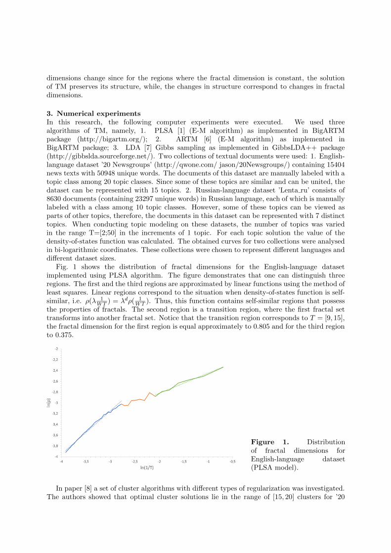
Fig. 1 shows the distribution of fractal dimensions for the English-language datasetimplemented using PLSA algorithm. The figure demonstrates that one can distinguish threeregions. The first and the third regions are approximated by linear functions using the method ofleast squares. Linear regions correspond to the situation when density-of-states function is self-similar, i.e. ρ(λ 1

WT ) = λdρ( 1WT ). Thus, this function contains self-similar regions that possess

the properties of fractals. The second region is a transition region, where the first fractal settransforms into another fractal set. Notice that the transition region corresponds to T = [9, 15],the fractal dimension for the first region is equal approximately to 0.805 and for the third regionto 0.375.

Figure 1. Distributionof fractal dimensions forEnglish-language dataset(PLSA model).

In paper [8] a set of cluster algorithms with different types of regularization was investigated.The authors showed that optimal cluster solutions lie in the range of [15, 20] clusters for ’20

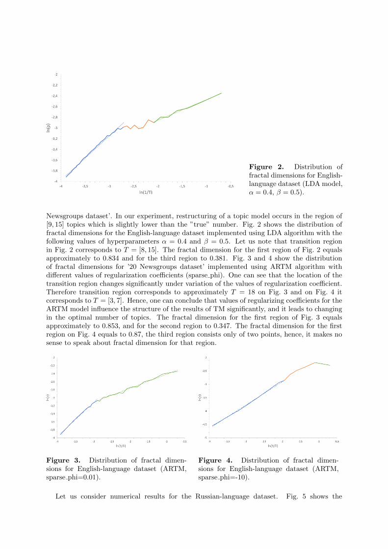
Figure 2. Distribution offractal dimensions for English-language dataset (LDA model,α = 0.4, β = 0.5).

Newsgroups dataset’. In our experiment, restructuring of a topic model occurs in the region of[9, 15] topics which is slightly lower than the ”true” number. Fig. 2 shows the distribution offractal dimensions for the English-language dataset implemented using LDA algorithm with thefollowing values of hyperparameters α = 0.4 and β = 0.5. Let us note that transition regionin Fig. 2 corresponds to T = [8, 15]. The fractal dimension for the first region of Fig. 2 equalsapproximately to 0.834 and for the third region to 0.381. Fig. 3 and 4 show the distributionof fractal dimensions for ’20 Newsgroups dataset’ implemented using ARTM algorithm withdifferent values of regularization coefficients (sparse phi). One can see that the location of thetransition region changes significantly under variation of the values of regularization coefficient.Therefore transition region corresponds to approximately T = 18 on Fig. 3 and on Fig. 4 itcorresponds to T = [3, 7]. Hence, one can conclude that values of regularizing coefficients for theARTM model influence the structure of the results of TM significantly, and it leads to changingin the optimal number of topics. The fractal dimension for the first region of Fig. 3 equalsapproximately to 0.853, and for the second region to 0.347. The fractal dimension for the firstregion on Fig. 4 equals to 0.87, the third region consists only of two points, hence, it makes nosense to speak about fractal dimension for that region.

Figure 3. Distribution of fractal dimen-sions for English-language dataset (ARTM,sparse phi=0.01).

Figure 4. Distribution of fractal dimen-sions for English-language dataset (ARTM,sparse phi=-10).

Let us consider numerical results for the Russian-language dataset. Fig. 5 shows the

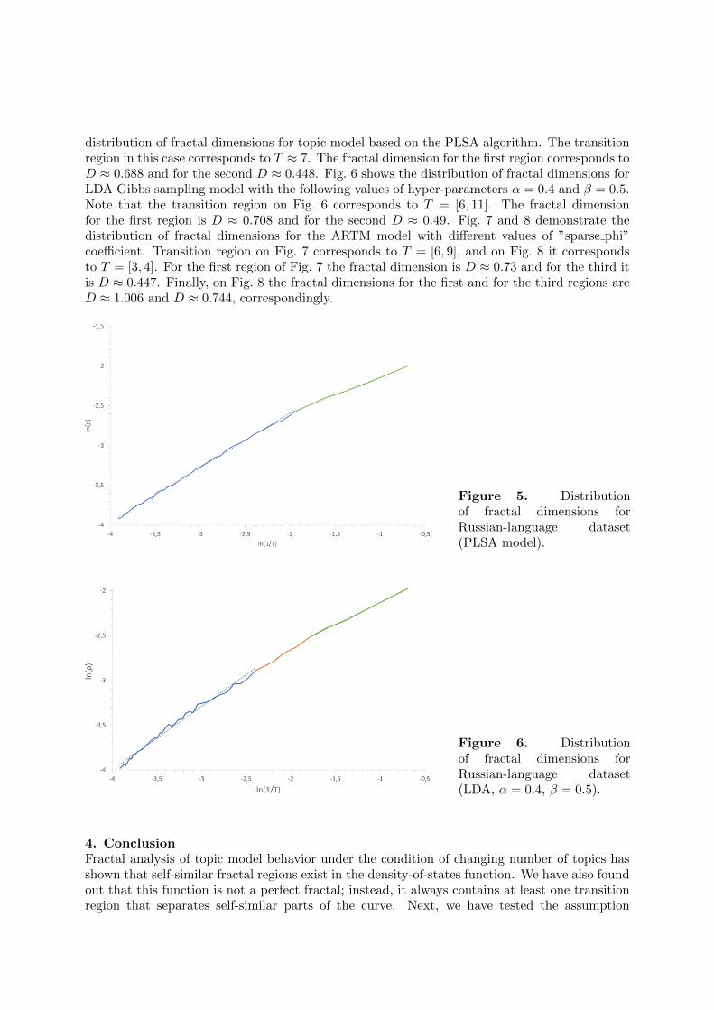
distribution of fractal dimensions for topic model based on the PLSA algorithm. The transitionregion in this case corresponds to T ≈ 7. The fractal dimension for the first region corresponds toD ≈ 0.688 and for the second D ≈ 0.448. Fig. 6 shows the distribution of fractal dimensions forLDA Gibbs sampling model with the following values of hyper-parameters α = 0.4 and β = 0.5.Note that the transition region on Fig. 6 corresponds to T = [6, 11]. The fractal dimensionfor the first region is D ≈ 0.708 and for the second D ≈ 0.49. Fig. 7 and 8 demonstrate thedistribution of fractal dimensions for the ARTM model with different values of ”sparse phi”coefficient. Transition region on Fig. 7 corresponds to T = [6, 9], and on Fig. 8 it correspondsto T = [3, 4]. For the first region of Fig. 7 the fractal dimension is D ≈ 0.73 and for the third itis D ≈ 0.447. Finally, on Fig. 8 the fractal dimensions for the first and for the third regions areD ≈ 1.006 and D ≈ 0.744, correspondingly.

Figure 5. Distributionof fractal dimensions forRussian-language dataset(PLSA model).

Figure 6. Distributionof fractal dimensions forRussian-language dataset(LDA, α = 0.4, β = 0.5).

4. ConclusionFractal analysis of topic model behavior under the condition of changing number of topics hasshown that self-similar fractal regions exist in the density-of-states function. We have also foundout that this function is not a perfect fractal; instead, it always contains at least one transitionregion that separates self-similar parts of the curve. Next, we have tested the assumption

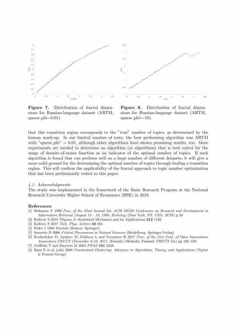
Figure 7. Distribution of fractal dimen-sions for Russian-language dataset (ARTM,sparse phi=0.01).

Figure 8. Distribution of fractal dimen-sions for Russian-language dataset (ARTM,sparse phi=-10).

that this transition region corresponds to the ”true” number of topics, as determined by thehuman mark-up. In our limited number of tests, the best performing algorithm was ARTMwith ”sparse phi” = 0.01, although other algorithms have shown promising results, too. Moreexperiments are needed to determine an algorithm (or algorithms) that is best suited for theusage of density-of-states function as an indicator of the optimal number of topics. If suchalgorithm is found that can perform well on a large number of different datasets, it will give amore solid ground for the determining the optimal number of topics through finding a transitionregion. This will confirm the applicability of the fractal approach to topic number optimizationthat has been preliminarily tested in this paper.

4.1. AcknowledgmentsThe study was implemented in the framework of the Basic Research Program at the NationalResearch University Higher School of Economics (HSE) in 2018.

References[1] Hofmann T 1999 Proc. of the 22nd Annual Int. ACM SIGIR Conference on Research and Development in

Information Retrieval (August 15 - 19, 1999, Berkeley) (New York, NY, USA: ACM) p 50[2] Koltcov S 2018 Physica A: Statistical Mechanics and its Applications 512 1192[3] Koltcov S 2017 Tech. Phys. Letters 43 584[4] Feder J 1988 Fractals (Boston: Springer)[5] Sornette D 2006 Critical Phenomena in Natural Sciences (Heidelberg: Springer-Verlag)[6] Kochedykov D, Apishev M, Golitsyn L and Vorontsov K 2017 Proc. of the 21st Conf. of Open Innovations

Association FRUCT (November 6-10, 2017, Helsinki) (Helsinki, Finland: FRUCT Oy) pp 182–193[7] Griffiths T and Steyvers M 2004 PNAS 101 5228[8] Basu S et al. (eds) 2008 Constrained Clustering: Advances in Algorithms, Theory, and Applications (Taylor

& Francis Group)