Embed Size (px)
Citation preview

Determining the Optimal Orientation of Orthotropic
Material for Maximizing Frequency Band Gaps
by
Dane Haystead
A thesis submitted in conformity with the requirementsfor the degree of Masters of Applied Science
Graduate Department of Aerospace Science and EngineeringUniversity of Toronto
Copyright c© 2012 by Dane Haystead

Abstract
Determining the Optimal Orientation of Orthotropic Material for Maximizing
Frequency Band Gaps
Dane Haystead
Masters of Applied Science
Graduate Department of Aerospace Science and Engineering
University of Toronto
2012
As the use of carbon fiber reinforced polymers (CFRP) increases in aerospace struc-
tures it is important to use this material in an efficient manner such that both the weight
and cost of the structure are minimized while maintaining its performance. To com-
bat undesirable vibrational characteristics of a structure an optimization program was
developed which takes advantage of the orthotropic nature of composite materials to
maximize eigenfrequency bandgaps. The results from the optimization process were then
fabricated and subjected to modal testing. The experiments show that local fiber angle
optimization is a valid method for modifying the natural frequencies of a structure with
the theoretical results generally predicting the performance of the optimized composite
plates.
ii

Acknowledgements
First and foremost I would like to thank my advisor, Dr. Craig Steeves, for all of his
support and time over the last two years. He allowed me to work at my own pace and
always provided valuable insight.
I would also like to thank my colleagues Richard Lee, Collins Ogundipe, and Bryan
Wright for always being available to bounce questions off of and for their help in the lab.
Finally, I would like to thank my parents for their continued support in my pursuit of
higher education.
iii

Contents
1 Introduction 1
2 Background 4
2.1 Finite Element Formulation . . . . . . . . . . . . . . . . . . . . . . . . . 4
2.1.1 Composite Laminates . . . . . . . . . . . . . . . . . . . . . . . . . 9
2.2 Optimization of Orthotropic Material Orientation . . . . . . . . . . . . . 13
2.2.1 Steepest Descent Method . . . . . . . . . . . . . . . . . . . . . . . 14
2.2.2 Sensitivity Analysis . . . . . . . . . . . . . . . . . . . . . . . . . . 15
2.2.3 Function Maximization . . . . . . . . . . . . . . . . . . . . . . . . 16
2.3 Modal Analysis . . . . . . . . . . . . . . . . . . . . . . . . . . . . . . . . 17
3 Optimization 21
3.1 Implementation . . . . . . . . . . . . . . . . . . . . . . . . . . . . . . . . 21
3.1.1 Parallelization . . . . . . . . . . . . . . . . . . . . . . . . . . . . . 24
3.2 Results . . . . . . . . . . . . . . . . . . . . . . . . . . . . . . . . . . . . . 26
3.2.1 Single Eigenfrequencies . . . . . . . . . . . . . . . . . . . . . . . . 29
3.2.2 Eigenfrequency Bandgaps . . . . . . . . . . . . . . . . . . . . . . 36
3.2.3 Other Eigenfrequency Gaps . . . . . . . . . . . . . . . . . . . . . 44
4 Modal Analysis 51
4.1 Testing Procedure . . . . . . . . . . . . . . . . . . . . . . . . . . . . . . . 51
iv

4.2 Fabrication . . . . . . . . . . . . . . . . . . . . . . . . . . . . . . . . . . 53
4.3 Results . . . . . . . . . . . . . . . . . . . . . . . . . . . . . . . . . . . . . 54
5 Conclusions 63
5.1 Recommendations . . . . . . . . . . . . . . . . . . . . . . . . . . . . . . . 65
Bibliography 67
v

List of Tables
3.1 Eigenfrequencies calculated from optimized results from maximization of
the 1st and 2nd eigenfrequencies . . . . . . . . . . . . . . . . . . . . . . . 37
3.2 Eigenfrequencies calculated from optimized results from maximization of
the 2nd and 3rd eigenfrequencies . . . . . . . . . . . . . . . . . . . . . . . 39
3.3 Eigenfrequencies calculated from optimized results from maximization of
the 3rd and 4th eigenfrequencies . . . . . . . . . . . . . . . . . . . . . . . 40
3.4 Eigenfrequencies calculated from optimized results from maximization of
the 4th and 5th eigenfrequencies . . . . . . . . . . . . . . . . . . . . . . . 42
3.5 Natural frequencies [Hz] calculated for the optimal fiber angles for the
maximization of the bandgap between the 5th and 6th eigenfrequencies . . 43
4.1 Predicted results from ABAQUS calculations for the 1− 2 bandgap max-
imization . . . . . . . . . . . . . . . . . . . . . . . . . . . . . . . . . . . . 56
4.2 Predicted results from ABAQUS calculations for the 2− 3 bandgap max-
imization . . . . . . . . . . . . . . . . . . . . . . . . . . . . . . . . . . . . 57
4.3 Predicted results from ABAQUS calculations for the 3− 4 bandgap max-
imization . . . . . . . . . . . . . . . . . . . . . . . . . . . . . . . . . . . . 59
4.4 Predicted results from ABAQUS calculations for the 4− 5 bandgap max-
imization . . . . . . . . . . . . . . . . . . . . . . . . . . . . . . . . . . . . 60
4.5 Predicted results from ABAQUS calculations for the 5− 6 bandgap max-
imization . . . . . . . . . . . . . . . . . . . . . . . . . . . . . . . . . . . . 61
vi

List of Figures
1.1 MBB beam before and after topology optimization . . . . . . . . . . . . 3
2.1 Unidirectional fiber element with fibers aligned parallel to the x-axis . . . 5
2.2 Rotated unidirectional ply . . . . . . . . . . . . . . . . . . . . . . . . . . 7
2.3 The method and notation used for calculating the ply thickness values, zk,
used in the A, B, and D matrix calculations . . . . . . . . . . . . . . . . 10
2.4 Impact hammer impulse and response discrete-time signal from aluminum
flat bar . . . . . . . . . . . . . . . . . . . . . . . . . . . . . . . . . . . . . 19
2.5 FRF of cantilevered aluminum flat bar . . . . . . . . . . . . . . . . . . . 20
3.1 Flowchart of optimization program . . . . . . . . . . . . . . . . . . . . . 23
3.2 Profile of Matlab optimization code . . . . . . . . . . . . . . . . . . . . . 24
3.3 Organization of parallel calculations . . . . . . . . . . . . . . . . . . . . . 25
3.4 The effect of parallelization on computation time for various mesh sizes . 26
3.5 24x8 element mesh on a 9x3 inch plate . . . . . . . . . . . . . . . . . . . 27
3.6 Unidirectional prepreg carbon fiber tensile test results . . . . . . . . . . . 28
3.7 Mode shapes for bending eigenfrequencies . . . . . . . . . . . . . . . . . 30
3.8 Optimized fiber angles for maximizing the frequencies associated with the
first three bending modes . . . . . . . . . . . . . . . . . . . . . . . . . . . 30
3.9 Convergence for the maximization of the 1st eigenfrequency from 45◦ start 31
3.10 Convergence for the maximization of the 3rd eigenfrequency from 45◦ start 31
vii

3.11 Convergence for the maximization of the 5th eigenfrequency from 45◦ start 32
3.12 Comparison of optimized fiber angles to mode shape for the 2nd eigenfre-
quency . . . . . . . . . . . . . . . . . . . . . . . . . . . . . . . . . . . . . 33
3.13 Convergence for the maximization of the 2nd eigenfrequency . . . . . . . 33
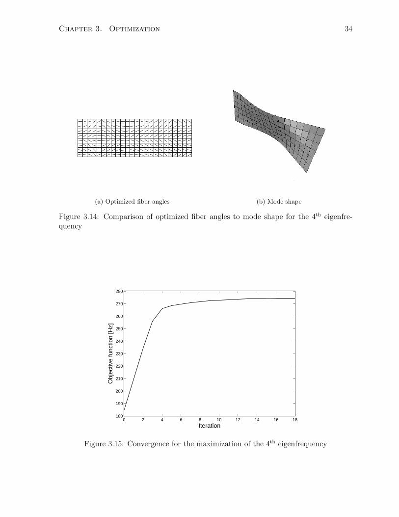
3.14 Comparison of optimized fiber angles to mode shape for the 4th eigenfre-
quency . . . . . . . . . . . . . . . . . . . . . . . . . . . . . . . . . . . . . 34
3.15 Convergence for the maximization of the 4th eigenfrequency . . . . . . . . 34
3.16 Comparison of optimized fiber angles to mode shape for the 6th eigenfre-
quency . . . . . . . . . . . . . . . . . . . . . . . . . . . . . . . . . . . . . 35
3.17 Convergence for the maximization of the 6th eigenfrequency . . . . . . . . 35
3.18 Results of optimization for maximization of the bandgap between the 1st
and 2nd eigenfrequencies . . . . . . . . . . . . . . . . . . . . . . . . . . . 36
3.19 Convergence for the maximization of the bandgap between the 1st and 2nd
eigenfrequencies . . . . . . . . . . . . . . . . . . . . . . . . . . . . . . . . 37
3.20 Results of optimization for maximization of the bandgap between the 2nd
and 3rd eigenfrequencies . . . . . . . . . . . . . . . . . . . . . . . . . . . 38
3.21 Convergence for the maximization of the bandgap between the 2nd and 3rd
eigenfrequencies . . . . . . . . . . . . . . . . . . . . . . . . . . . . . . . . 39
3.22 Results of optimization for maximization of the bandgap between the 3rd
and 4th eigenfrequencies . . . . . . . . . . . . . . . . . . . . . . . . . . . 40
3.23 Convergence for the maximization of the bandgap between the 3rd and 4th
eigenfrequencies . . . . . . . . . . . . . . . . . . . . . . . . . . . . . . . . 40
3.24 Results of optimization for maximization of the bandgap between the 4th
and 5th eigenfrequencies . . . . . . . . . . . . . . . . . . . . . . . . . . . 41
3.25 Convergence for the maximization of the bandgap between the 4th and 5th
eigenfrequencies . . . . . . . . . . . . . . . . . . . . . . . . . . . . . . . . 42
viii

3.26 Results of optimization for maximization of the bandgap between the 5th
and 6th eigenfrequencies . . . . . . . . . . . . . . . . . . . . . . . . . . . 43
3.27 Convergence for the maximization of the bandgap between the 5th and 6th
eigenfrequencies . . . . . . . . . . . . . . . . . . . . . . . . . . . . . . . . 43
3.28 Optimization results for the maximization of the 1− 3 gap . . . . . . . . 45
3.29 Optimization results for the maximization of the 1− 4 gap . . . . . . . . 45
3.30 Optimization results for the maximization of the 2− 4 gap . . . . . . . . 46
3.31 Optimization results for the maximization of the 1− 5 gap . . . . . . . . 46
3.32 Optimization results for the maximization of the 2− 5 gap . . . . . . . . 47
3.33 Optimization results for the maximization of the 3− 5 gap . . . . . . . . 47
3.34 Optimization results for the maximization of the 1− 6 gap . . . . . . . . 49
3.35 Optimization results for the maximization of the 2− 6 bandgap . . . . . 49
3.36 Optimization results for the maximization of the 3− 6 bandgap . . . . . 50
3.37 Optimization results for the maximization of the 4− 6 bandgap . . . . . 50
4.2 Modal testing hardware shown with a pencil for scale . . . . . . . . . . . 52
4.1 Labview block diagram for reading modal analysis data and saving to a file 52
4.3 Accelerometer attached to plate ready for testing . . . . . . . . . . . . . 53
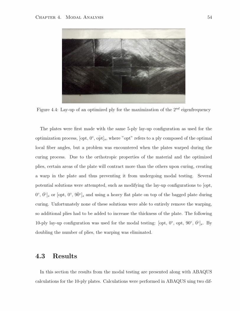
4.4 Lay-up of an optimized ply for the maximization of the 2nd eigenfrequency 54
4.5 Frequency response funtion calculated from the accelerometer attached to
the top-center of the plate with a maximized 1− 2 bandgap . . . . . . . 55
4.6 Frequency response funtion calculated from the accelerometer attached to
the top-right corner of the plate with a maximized 1− 2 bandgap . . . . 56
4.7 Frequency response funtion calculated from the accelerometer attached to
the top-center of the plate with a maximized 2− 3 bandgap . . . . . . . 57
4.8 Frequency response funtion calculated from the accelerometer attached to
the top-right corner of the plate with a maximized 2− 3 bandgap . . . . 57
ix

4.9 Frequency response funtion calculated from the accelerometer attached to
the top-center of the plate with a maximized 3− 4 bandgap . . . . . . . 58
4.10 Frequency response funtion calculated from the accelerometer attached to
the top-right corner of the plate with a maximized 3− 4 bandgap . . . . 58
4.11 Frequency response funtion calculated from the accelerometer attached to
the top-center of the plate with a maximized 4− 5 bandgap . . . . . . . 59
4.12 Frequency response funtion calculated from the accelerometer attached to
the top-center of the plate with a maximized 4− 5 bandgap . . . . . . . 60
4.13 Frequency response funtion calculated from the accelerometer attached to
the top-center of the plate with a maximized 5− 6 bandgap . . . . . . . 61
4.14 Frequency response funtion calculated from the accelerometer attached to
the top-right corner of the plate with a maximized 5− 6 bandgap . . . . 61
x

Chapter 1
Introduction
As the use of carbon fiber reinforced polymers (CFRP) increases in aerospace structures
it is important to use this material in an efficient manner such that both the weight
and cost of the structure are minimized while maintaining its performance. In some
cases these structures may have undesirable vibrational characteristics while also being
geometrically constrained, creating a unique problem. One possible solution is to take
advantage of the orthotropic properties of composite materials and use them to modify
the vibrational characteristics while maintaining the overall geometry of the part. The
goal of the research presented in this thesis is to develop a method to optimize the
fiber orientations throughout thin rectangular composite plates for the maximization of
specific eigenfrequencies and eigenfrequency bandgaps.
Fiber reinforced polymers are popular in the aerospace industry due to their high
strength to weight ratio and the ever increasing demands on aircraft performance. Com-
posite structures are fabricated by laying up many layers of fibers (either woven or un-
woven) into the desired final shape, bonding them together with resin then curing the
part. The final properties of a composite structure can depend on several factors of the
construction, such as orientation of orthotropic plies, ply thickness, stacking sequence,
and material properties of both the reinforcement and matrix (resin). This high degree of
1

Chapter 1. Introduction 2
variablility can be taken advantage of to provide an optimal solution for a given scenario,
and this can be accomplished using structural optimization.
Structural optimization can take many forms, from shape optimization where, for
example, the dimensions of the cross-section of trusses in a structure are optimized to
minimize bending stress, to topology optimization, where the layout of material in a
design domain is optimized for minimum compliance under the given loads and boundary
conditions. While there are many different uses for structural optimization, the general
process for finding the optimal design follows the same method.
Topology optimization is a method for determining the optimal layout of material in
a specified design domain which satisfies a set of loading and boundary conditions and
produces a final product that meets all of the specified requirements. It is a very useful
tool in industries where the efficient use of material (reducing weight) is important, such
as the aerospace and automotive industries. Typically it is used to determine the optimal
layout of material in a structure so that the compliance of the structure is minimized while
a constraint on mass is satisfied [15], but it can be can also be applied to wide variety
of scenarios such as compliant mechanisms for microelectromechanical devices[18], smart
materials [16][17], and maximizing eigenfrequencies and frequency band gaps [10][12].
Optimization of orthotropic material orientation has many similarities with topology
optimization; they both are based on a discretized domain where the material properties
of the elements are dependent upon the design variables, they share many of the same
objective functions, and they both are methods which attempt to determine the most
efficient use of material.

Chapter 1. Introduction 3
(a) MBB beam domain (b) Optimized topology of MBB beam
Figure 1.1: MBB beam before and after topology optimization
The design variable is major difference between the two. Topology optimization uses
the material density of the elements, while fiber angle optimziation uses the angle of the
principal material direction. As stated earlier, the goal of both is to find the most efficient
use of material under the given conditions, and in the case of fiber angle optimization,
this means getting the most benefit from the from the fibers at every point throughout
the structure. Having fibers oriented incorrectly can be considered an inefficient use of
resources and therefore a waste.
The objective of the thesis is to develop a gradient-based optimization method to de-
termine the optimal orientation of orthotropic material to maximize frequency band gaps
in a structure. The optimization method will then be applied to composite laminated
plates and the final optimized designs will be fabricated and tested. The next chapter
will provide background information on the mathematical methods used to model the
behaviour of structures composed of orthotropic material as well as the optimization
process used to maximize the frequency band gaps of the composite structures. Chapter
three applies these methods to laminated composite plates under various boundary con-
ditions and the optimized fiber orientations are discussed. In Chapter four the results
from the optimzation are verified using commercial software and then compared to the
results from the modal analysis of the optimized physical specimens. The conclusions
and recommendations of the thesis are provided in Chapter five.

Chapter 2
Background
2.1 Finite Element Formulation
To determine the vibrational characteristics of the laminated composite plate with
variable fiber angles, the finite element method is used. The plate is discretized as
a set of 4-noded plate elements, with each element having its own fiber angle. The
vibrational characteristics are determined by solving for the non-trivial solution to the
generalized eigenproblem, which is a function of the stiffness and mass matrices, K and
M , respectively.
Kφi = λiMφi (2.1)
The other values in the generalized eigenproblem are λi, the eigenvalue, and φi, the
eigenvector. The eigenenfrequency (natural frequency), ωi, is the sqaure root of the
eigenvalue:
ωi =√
λi (2.2)
The generalized eigenproblem can then be simplified to:
4

Chapter 2. Background 5
(K − ω2iM)φi = 0 (2.3)
The K and M matrices are dependent on the properties of the elements used in the
discretization of the plate. The optimization of fiber angles was performed separately
on two different plate element formulations. Fiber angles were first optimized using 4-
noded orthotropic plate elements which model a single ply. The second type of plate
element used takes into account the fiber angles of all the orthotropic plies to produce an
approximation of a laminated composite plate where the properties of the elements are
calculated using First Order Shear Deformation Theory (FSDT), which is an extension
of Composite Laminate Theory (CLT) [9][14]. This finite element formulation will be
discussed further in Section 2.1.1.
A material is orthotropic when is has three orthogonal planes of symmetry; in the case
of a unidirectional lamina, the material symmetry planes are parallel and transverse to
the fiber directions. A two-dimensional representation of a unidirectional fiber element
can be seen in Figure 2.1.
Figure 2.1: Unidirectional fiber element with fibers aligned parallel to the x-axis
Hooke’s Law for an anisotropic material can be written (in contracted form) as
σi = Cijǫj , (2.4)

Chapter 2. Background 6
where σi are the stress components and ǫj are the strain components, while Cij are the
material coefficients [14][11]. For orthotropic materials, the number of material coeffi-
cients can be reduced from 21 to 9. This results in Equation (2.5).
σ1
σ2
σ3
τ23
τ31
τ12
=
C11 C12 C13
C12 C22 C23
C13 C23 C33
C44
C55
C66
ǫ1
ǫ2
ǫ3
γ23
γ31
γ12
(2.5)
Laminated composite plates are thin and therefore in a plane state of stress and the
transverse normal stress, σ3, can be neglected. The stress-strain relations in this state
are referred to as the plane-stress constitutive relations, and they are written as
σ1
σ2
σ6
=
Q11 Q12 0
Q12 Q22 0
0 0 Q66
ǫ1
ǫ2
ǫ6
, (2.6)
and
σ4
σ5
=
Q44 0
0 Q55
ǫ4
ǫ5
, (2.7)
where Qij are the plane stress reduced stiffnesses. When multiple lamina are present, the
(k) notation is added to denote the ply that the plane stress-reduced stiffness belongs to.
The Q(k)ij values are calculated with the following equations:

Chapter 2. Background 7
Q(k)11 =
E(k)1
1− ν(k)12 ν
(k)21
, (2.8)
Q(k)12 =
ν(k)12 E
(k)2
1− ν(k)12 ν
(k)21
, (2.9)
Q(k)22 =
E(k)2
1− ν(k)12 ν
(k)21
, (2.10)
Q(k)44 = G
(k)23 , (2.11)
Q(k)55 = G
(k)13 , (2.12)
Q(k)66 = G
(k)12 , (2.13)
where
ν21 =ν12E2
E1
(2.14)
When the local coordinates of the orthotropic material are not aligned with the global
coordinates, as shown in Figure 2.2, the local material coefficients are multiplied by
transformation matrices to calculate the global material coefficients, as seen in Equation
(2.15).
ϴ
Figure 2.2: Rotated unidirectional ply
[C̄] = [T ][C][T ]T (2.15)
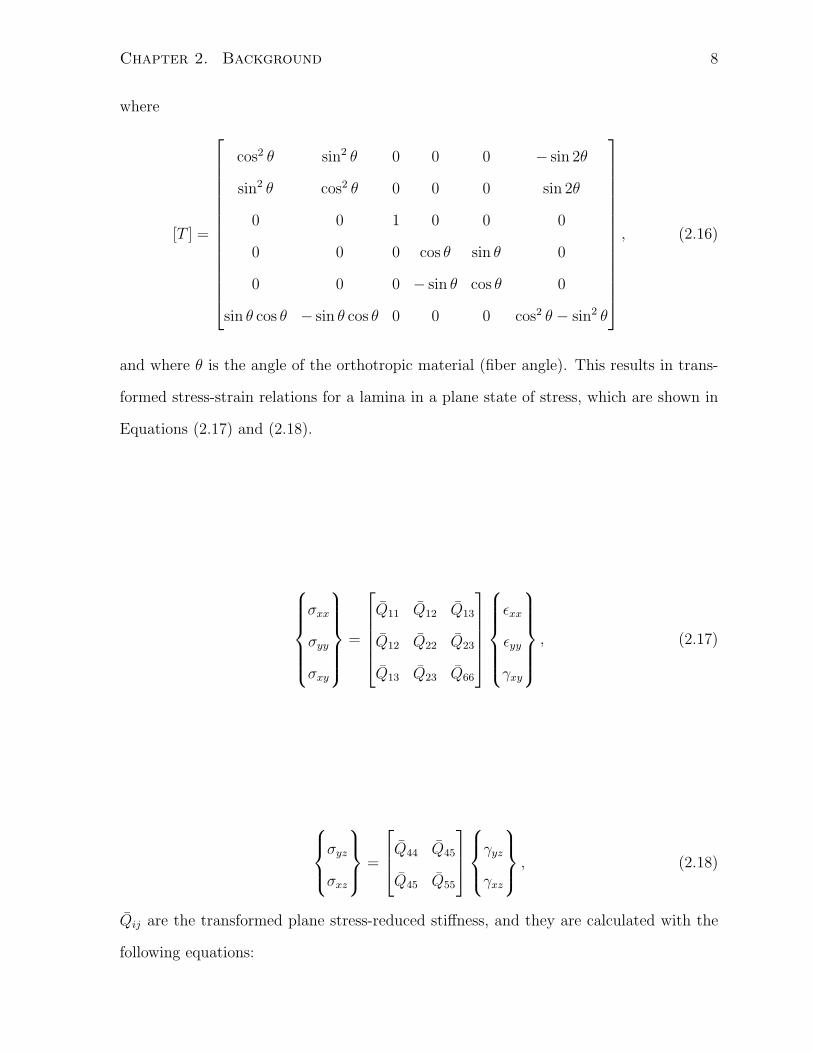
Chapter 2. Background 8
where
[T ] =
cos2 θ sin2 θ 0 0 0 − sin 2θ
sin2 θ cos2 θ 0 0 0 sin 2θ
0 0 1 0 0 0
0 0 0 cos θ sin θ 0
0 0 0 − sin θ cos θ 0
sin θ cos θ − sin θ cos θ 0 0 0 cos2 θ − sin2 θ
, (2.16)
and where θ is the angle of the orthotropic material (fiber angle). This results in trans-
formed stress-strain relations for a lamina in a plane state of stress, which are shown in
Equations (2.17) and (2.18).
σxx
σyy
σxy
=
Q̄11 Q̄12 Q̄13
Q̄12 Q̄22 Q̄23
Q̄13 Q̄23 Q̄66
ǫxx
ǫyy
γxy
, (2.17)
σyz
σxz
=
Q̄44 Q̄45
Q̄45 Q̄55
γyz
γxz
, (2.18)
Q̄ij are the transformed plane stress-reduced stiffness, and they are calculated with the
following equations:

Chapter 2. Background 9
Q̄11 = Q11 cos4 θ + 2(Q12 + 2Q66) sin
2 θ cos2 θ +Q22 sin4 θ (2.19)
Q̄12 = (Q11 +Q22 − 4Q66) sin2 θ cos2 θ +Q12(sin
4 θ + cos4 θ) (2.20)
Q̄22 = Q11 sin4 θ + 2(Q12 + 2Q66) sin
2 θ cos2 θ +Q22 cos4 θ (2.21)
Q̄16 = (Q11 −Q12 − 2Q66) sin θ cos3 θ + (Q12 −Q22 + 2Q66) sin
3 θ cos θ (2.22)
Q̄26 = (Q11 −Q12 − 2Q66) sin3 θ cos θ + (Q12 −Q22 + 2Q66) sin θ cos
3 θ (2.23)
Q̄66 = (Q11 +Q22 − 2Q12 − 2Q66) sin2 θ cos2 θ +Q66(sin
4 θ + cos4 θ) (2.24)
Q̄44 = Q44 cos2 θ +Q55 sin
2 θ (2.25)
Q̄45 = (Q55 −Q44) cos θ sin θ (2.26)
Q̄55 = Q55 cos2 θ +Q44 sin
2 θ (2.27)
2.1.1 Composite Laminates
As mentioned earlier, FSDT is an extension of CLT, which itself is an extension of
Kirchoff plate theory applied to composite plates. Specifically, FSDT includes transverse
shear strains, whereas CLT does not. Both FSDT and CLT belong to a group of theories
called Equavalent Single Layer theories (ESL), which assumes the laminated plate is a
single layer with complex constitutive behaviour. This is one of three major approaches
for performing analyses of laminated plates; the others being: 3-D elasticity theories and
Multiple model methods.
To approximate multiple plies as an equivalent single layer three stiffness matrices are
calculated as a function of the transformed plane stress-reduced stiffnesses, Q̄ij, and the
ply thicknesses. These matrices are: Aij , the extensional stiffnesses, Dij , the bending
stiffnesses, and Bij, the bending-extensional coupling stiffnesses. They are calculated
using Equations (2.28-2.30), where the zk values are calculated based on the ply notation

Chapter 2. Background 10
scheme in Figure 2.3.
Aij =N∑
k=1
Q̄(k)ij (zk+1 − zk), (2.28)
Bij =1
2
N∑
k=1
Q̄(k)ij (z2k+1 − z2k), (2.29)
Dij =1
3
N∑
k=1
Q̄(k)ij (z3k+1 − z3k), (2.30)
k = 1
k = 2
k = N
Figure 2.3: The method and notation used for calculating the ply thickness values, zk,used in the A, B, and D matrix calculations
The stiffness matrices are calculated for each element in the finite element formulation.
These matrices are then used to calculate the various membrane, bending, and shear
elemental stiffness matrices which are then summed to produce the overall elemental
stiffness matrix [K](e), as shown in Equation (2.31).
K(e) = K(e)mm +K
(e)mb +K
(e)bm +K
(e)bb +K(e)
ss (2.31)
The components of the elemental stiffness matrix are the K(e)mm, the membrane portion of
the stiffness matrix, K(e)mb and K
(e)bm, the membrane-bending coupling components, K
(e)bb ,

Chapter 2. Background 11
the bending component, and lastly K(e)ss , the shear component. They are calculated with
the following equations:
K(e)mm =
N∑
k=1
∫
A
BTmABm(zk+1 − zk)dA (2.32)
K(e)mb =
N∑
k=1
∫
A
BTmBBb
1
2(z2k+1 − z2k)dA (2.33)
K(e)bm =
N∑
k=1
∫
A
BTb BBm
1
2(z2k+1 − z2k)dA (2.34)
K(e)bb =
N∑
k=1
∫
A
BTb DBb
1
3(z3k+1 − z3k)dA (2.35)
K(e)ss =
N∑
k=1
∫
A
BTs SBs(zk+1 − zk)dA (2.36)
where
[A] =
A11 A12 A13
A12 A22 A23
A13 A23 A66
(2.37)
[S] =
A44 A45
A45 A55
(2.38)
[Bm](e) =
∂Nj
∂x0 0 0 0
0∂Nj
∂y0 0 0
∂Nj
∂y
∂Nj
∂x0 0 0
(2.39)
[Bb](e) =
0 0 0∂Nj
∂x0
0 0 0 0∂Nj
∂y
0 0 0∂Nj
∂y
∂Nj
∂x
(2.40)
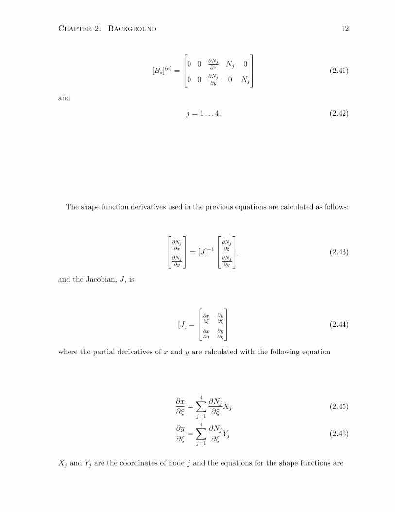
Chapter 2. Background 12
[Bs](e) =
0 0∂Nj
∂xNj 0
0 0∂Nj
∂y0 Nj
(2.41)
and
j = 1 . . . 4. (2.42)
The shape function derivatives used in the previous equations are calculated as follows:
∂Nj
∂x
∂Nj
∂y
= [J ]−1
∂Nj
∂ξ
∂Nj
∂η
, (2.43)
and the Jacobian, J , is
[J ] =
∂x∂ξ
∂y
∂ξ
∂x∂η
∂y
∂η
(2.44)
where the partial derivatives of x and y are calculated with the following equation
∂x
∂ξ=
4∑
j=1
∂Nj
∂ξXj (2.45)
∂y
∂ξ=
4∑
j=1
∂Nj
∂ξYj (2.46)
Xj and Yj are the coordinates of node j and the equations for the shape functions are

Chapter 2. Background 13
N1 =1
4[(1− ξ)(1− η)] (2.47)
N2 =1
4[(1 + ξ)(1− η)] (2.48)
N3 =1
4[(1 + ξ)(1 + η)] (2.49)
N4 =1
4[(1− ξ)(1 + η)] (2.50)
where ξ and η are the values from the Gaussian quadrature numerical integration method.
The mass matrix is calculated using the consistent mass matrix formulation. Equation
(2.51) is the equation for the elemental mass matrix and the global mass matrix is
assembled in the same manner as the global stiffness matrix
M e =
∫
ρNTNdV. (2.51)
With the calculations of the global mass and stiffness matrices complete, the general
eigenproblem, Equation (2.3), can be solved. Many numerical methods for solving this
problem exist, but the number of solution options available will vary based on the linear
algebra library used. The method used in this thesis is symmetric bidiagonalization
followed by QR reduction. This will be expanded upon further in Chapter 3.
2.2 Optimization of Orthotropic Material Orienta-
tion
Optimization is a mathematical process in which an objective function is minimized or
maximized while satisfying any imposed constraints. The optimization problem encoun-
tered in this thesis is the maximization of eigenfrequencies and eigenfrequency band gaps

Chapter 2. Background 14
in plates constructed from orthotropic material (unidirectional pre-preg carbon fiber).
The optimization problem can be formulated as:
maximize : ωi(θn), (2.52)
subject to : (K − ω2iM)φi = 0 (2.53)
There are numerous optimiaztion methods, ranging from evolutionary optimization to
gradient-based methods, each with their own strengths and weaknesses. The optimiza-
tion problem encountered in this thesis requires a large number of design variables, and
therefore only gradient based methods were considered. Of the gradient-based methods,
the steepest descent method was selected for use.
2.2.1 Steepest Descent Method
The steepest descent method was selected for its simplicity and ease of implementation.
As described in its name, this method calculates the steepest descent direction and then
calculates the size of step to take in that direction. To determine the maximum, instead
of the minimum, a small modification had to be made to this algorithm. Specifically,
calculating the steepest ascent instead of steepest descent. The major steps of this
algorithm are as follows:
1. Set starting point for design variables: θ0n, n = 1, 2, . . . N ,
2. Solve for objective function, f(θn),
3. Calculate gradient, g(θ) = ∇f(θn), and then ascent direction, pi = g(θn)/||g(θn)||,
4. Calculate step size αi in direction of pi using line search method,
5. Update design variables, θi+1n = θin + αipi,

Chapter 2. Background 15
6. Solve for new objective function. Stop if convergence criteria are satisfied, otherwise
i = i+ 1 and return to step 3.
where θn is the vector of fiber angles, N is the number of elements, and i is the current
iteration number. The sensitivity analysis, step size calculations, and convergence criteria
can vary depending on the user’s requirements. The sensitivity analysis and line search
methods used in this thesis will be expanded upon in the upcoming subsections. The
convergence criteria used determines convergence based on the magnitude of successive
changes in the objective function falling under a user defined limit. The equation is:
|f(θi+1n − θin)| ≤ ǫa + ǫr|f(θin)|, (2.54)
where ǫa is the absolute tolerance, which is set to ǫa = 10−6, and ǫr is the relative
tolerance, which is set at ǫr = 0.001. If this convergence criterion is satisfied for three
successive iterations, the optimization process has converged and the program will break
out of the iterative optimization loop.
2.2.2 Sensitivity Analysis
Gradient-based optimization methods depend on the sensitivity analysis to calculate
the gradients that are integral to the optimization process. The gradients are the deriva-
tives of the objective function(s) with respect to the design variables, and they are cal-
culated using the finite difference method in this thesis. It is not a very efficient method
and it is only a first order approximation, but it is simple to implement and easy to
parallelize. The equation is:
df
dxi
=f(xi + h)− f(xi)
h, (2.55)
where h is the finite difference interval. Its concurrency results from its ability to calculate
the derivative with respect to a design variable independently from all other derivative

Chapter 2. Background 16
calculations. The results of parallelization will be presented in Section 3.1.1.
2.2.3 Function Maximization
The golden section search method is used to calculate the maximium step size, αk, for
the optimization program to take in the steepest ascent direction. This method begins
by bracketing a search interval, [a, b], then two initial points, α1 and α2, are calculated
using the golden ratio, ϕ = (1 +√5)/2 ≃ 0.618. The starting α values are calculated as
follows:
α1 = a+ (b− a)(1− ϕ)
α2 = a+ (b− a)ϕ
The iterative proces starts by evaluating the objective function, f(θkn + αkpk) = f(α),
for the initial α values, then proceeds to reduce the search interval for the optimal value
of α using the golden ratio ϕ. This continues until the size of the search interval satisfies
the convergence criterion, ǫ, which is a limit on the minimum size. The algorithm is as
follows:
For the optimziation performed in this thesis, the convergence criterion is typically
set to ǫ = 0.1. With the golden search complete the design variables are updated and
the optimization process starts its next iteration.

Chapter 2. Background 17
while |f(α1)− f(α2)| ≥ ǫ doif (f(α1) ≥ f(α2) thena = α1α1 = α2
f(α1) = f(α2)α2 = a+ (b− a)ϕRecalculate f(α2)
else
b = α2
α2 = α1
f(α2) = f(α1)α1 = a+ (b− a)(1− ϕ)Recalculate f(α1)
end if
end while
2.3 Modal Analysis
In order to validate the optimization calculations, plates will be fabricated from uni-
directional prepreg carbon fiber tape and subjected to modal testing to determine their
natural frequencies. Modal analysis is a process in which the dynamic properties, such
as natural frequencies and damping, of a structure are determined by exciting the struc-
ture and measuring its response. Various methods are available for both excitation and
measurement.
Two popular excitation methods are the shaker and impact hammer. For small objects,
such as the plates that will be tested for this thesis, a shaker would attach to the structure
through an armature called a stinger which transmits the force from the shaker to the
structure. The excitation produced by a shaker is controlled by an input signal which is
set by the user. Common modal testing signals include a swept sine and random frequency
vibration profiles. A force transducer embedded in the shaker is used to measure the force
input. The impact hammer is used to provide an impulse to the structure which excites a
range of vibration modes, with the contact time of the hammer tip inversely proportional
to the size of the range of frequencies excited. An ideal impact would have an infinitely

Chapter 2. Background 18
small contact time which would provide the perfect impulse and excite all modes of
vibration with equal energy. The impact force is measure by a transducer located in the
hammer tip. The modal testing performed for in this thesis will use an impact hammer.
Two methods exist for measuring the response of the structure. One is the use of a
laser vibrometer which can measure the response at a single point or multiple points
simultaneously, depending on the device. The more common method of response mea-
surement is to use an accelerometer, which is what will be used in this thesis. Both
the force transducer and accelerometer provide an analog voltage signal which is sent
to the data aquisition system for signal conditioning and analog to digital conversion
(ADC). The ADC converts the continuous-time signal to a discrete-time signal and this
is the data that can be viewed and analyzed. When sampling the response signal it is
neccessary to remember that the highest measured frequency is one half of the sample
frequency, as shown in Equation (2.56). This is known as the Nyquist frequency. Figure
2.4 shows an example of the discrete time signal recorded from the impact and response
on a cantilevered aluminum flat bar.
FN =Fs
2, (2.56)
where FN is the Nyquist frequency and Fs is the sampling frequency.
To determine the natural frequencies of the tested structure, the discrete-time data
needs to be analyzed in the frequency domain. To convert the data to the frequency
domain, the fast Fourier transform (FFT) algorithm is used to calculate the discrete
Fourier transform (DFT). The frequency response of the structure can be determined by
calculating the frequency response function (FRF), H(f), as shown in Equation 2.57 [8].
H(f) =Sxy
Sxx
, (2.57)

Chapter 2. Background 19
0 1 2 3 4 5 6 7 8 9 10−10
0
10
20
30
40
50Impact Hammer Force Impulse
Time (s)
For
ce (
N)
(a) Impact hammer impulse
0 1 2 3 4 5 6 7 8 9 10−8
−6
−4
−2
0
2
4
6Accelerometer Response
Time (s)
Acc
eler
atio
n (g
)
(b) Response of aluminum bar
Figure 2.4: Impact hammer impulse and response discrete-time signal from aluminumflat bar
where Sxx is the power spectrum of the excitation signal and Sxy is the cross power
spectrum. The equations for the power spectra are:
Sxx =FFT (x)× FFT ∗(x)
N2, (2.58)
Sxy =FFT (y)× FFT ∗(x)
N2, (2.59)
where the asterisk after FFT denotes that the conjugate is used, x and y are the exci-
tation and response data, respectively, and N is the number of samples in the data set.
The frequency response function derived from the data presented in Figure 2.4 is shown
in Figure 2.5. Using commercial FEA software, the first four natural frequencies of the
bar were calculated to be: 27.1, 169.8, 171.3, and 474.8 Hz, which approximately matches
up with the peaks in the FRF. To obtain a better estimate of the natural frequencies
calculated in the FRF it is possible to apply a modal parameter extraction technique,
but its accuracy may be limited by the amount of noise present in the signal.

Chapter 2. Background 20
0 50 100 150 200 250 300 350 400 450 500−50
−40
−30
−20
−10
0
10
20
30
40
Frequency [Hz]
Am
plitu
de [d
B]
ExperimentalPredicted
Figure 2.5: FRF of cantilevered aluminum flat bar

Chapter 3
Optimization
3.1 Implementation
The optimization program was written in C/C++ and uses the GNU Scientific Li-
brary (GSL) for handling of the matrices, vectors, and linear algebra [1]. It optimizes
the fiber orientations throughout a rectangular plate for the maximization of specified
eigenfrequencies or eigenfrequency band gaps. The plate dimensions, ply thickness, ply
configuration (which plies are optimized and which ones remain unidirectional), material
properties, number of elements to use, boundary conditions, and objective function are
all user specified. Ply thickness is constant for all plies.
The problem is first initialized by defining the dimensions of the plate, xDim and yDim,
and the number of elements to use nelx and nely. These values are used as inputs into
the quadmesh() function which calculates the node coordinates and constructs elements
from these nodes, both of which are stored in a GSL matrix structure, nodeCoordinates
and elementNodes, respectively. With the discretization complete only the material
properties and ply configuration need to be set before the finite element calculations can
begin. Both the stiffness and mass matrices, K and M , are GSL matrices and they
are constructed with the CLT stiffness matrix() and CLT mass matrix() functions,
21

Chapter 3. Optimization 22
respectively.
The boundary conditions are set by the BC type variable. This variable is a string
and it is used as an input into the function CLT bc() which calculates the fixed nodes
and their degrees of freedom for a rectangular plate. The fixed degrees of freedom are
then eliminated from the stiffness and mass matrices before calculating the objective
function. Four steps are required to solve the general eigenproblem using GSL functions
and they are all contained within the function called eigensolve() which returns the
objective function as a double. First, a vector, matrix, and workspace are initialized. The
vector and matrix, eval and evec respectively, are used to store the final eigenvalues
and eigenvectors, and the workspace, w, is used in the calculations. To solve for the
eigenvalues and eigenvectors, the function gsl eigen gensymmv() is called to solve the
real general symmetric-definite eigensystem, as defined in Equation (2.1), and it has
the stiffness and mass matrices along with eval, evec, and w as arguments. A GSL
sorting function, gsl eigen gensymmv sort(), is then used to sort the eigenvalues and
eigenvectors. The eigenfreqeuncies are calculated by finding the root of the eigenvalues as
shown in Equation(2.2), and the units of the frequencies are radians per second. Lastly,
the relevant value, specified by the eigNumber variable which is an input argument, is
returned.
Two functions comprise the majority of computational load in the optimization portion
of the program. These are the gradient function, CLT grad(), which calculates the sensi-
tivities of each element, and the golden search function, CLT golden(), which calculates
the optimal step size using the golden section method. The optimization calculations are
contained within a while loop which is set to break if the convergence criteria are met.
As discussed earlier in Chapter 2, the gradients (sensivities) are calculated using the finite
difference method, which is shown in Equation (2.55). These gradients are used to find
the ascent direction, which is the direction the design variables have to travel to increase

Chapter 3. Optimization 23
the objective function. The golden section search function, CLT golden(), calculates the
size of step to take in the ascent direction. The new objective function is then compared
to the old one and is judged on whether it is coverging to a solution. If the objective
function has converged, the program breaks out of the optimization calculations and
writes the final fiber angles into a csv file which can then be plotted in Matlab.
Initialize FE domain
Set composite and lay-up properties
Calculate stiffness matrix, mass matrix, and
boundary conditions
Solve general eigenproblem to calculate
objective function
Optimized?
Start optimization
Gradient calculations
Step size calculations
Update design variable and recalculate
objective function
Output data to file
Yes
No
Figure 3.1: Flowchart of optimization program

Chapter 3. Optimization 24
3.1.1 Parallelization
Since the sensitivity of each element can be calculated independently from the rest,
the gradient calculations are a prime candidate for parallelization. Additionally, the
gradient calculations comprise of approximately 80% of the computational load when the
optimization program is run in serial, according to the profiling done in Matlab shown
in Figure 3.1.1, and therefore the addition of parallelized gradient calculations should
provide a signifcant decrease in computational time. This will also allow for optimizing
plates with a higher resolution mesh within reasonable time constraints. To make the
most of the concurrency of the gradient calculations, the optimization program was run
on the General Purpose Cluster (GPC) on SciNet.
Figure 3.2: Profile of Matlab optimization code
The parallelized gradient calculations were performed using a hybrid OpenMP/MPI
approach. Open MPI is an open source message passing interface (MPI) library which
was used to communicate between nodes on the GPC [2]. OpenMP is an API for shared

Chapter 3. Optimization 25
memory parallel processing and it was used for perfroming parallel calculations across
the processors of each node [3]. An example of the parallelization process using 3 nodes
is shown in Figure 3.1.1.
Main process
Node Node Node
Cores Cores Cores
MPI
OpenMP
Figure 3.3: Organization of parallel calculations
To demonstrate the performance gained from the use of parallel programming the
optimization program was run with varying numbers of nodes (each node containing 8
processors). Data was collected for two different meshes of the plate, 18x6 and 24x8
elements, and plotted in Figure 3.4. From these plots it can be seen that the use of
parallel processing greatly reduces the computational time required by the optimization
program.

Chapter 3. Optimization 26
0 10 20 30 40 50 60 70 80 90 1001
1.5
2
2.5
Number of Processors
Min
utes
per
Iter
atio
n
(a) 18x6 element mesh
0 10 20 30 40 50 60 70 80 90 1004
6
8
10
12
14
16
18
20
22
24
Number of Processors
Min
utes
per
Iter
atio
n
(b) 24x8 element mesh
Figure 3.4: The effect of parallelization on computation time for various mesh sizes
3.2 Results
Plates of the size 9” by 3” were optimized with varying mesh sizes, ranging from
18x6 up to 30x10, as shown in Figure 3.2. The objective functions maximized the 1st
to 6th eigenfrequencies and also all eigenfrequency band-gaps within that range. The
orthotropic material used in the simulations is an approximation of the unidirectional
prepreg carbon fiber which will be used to fabricate the test samples. These material
properties were also used when verifiying the optimization results with the commercial
FEA software package ABAQUS. The results from the ABAQUS calculations will be
presented with the optimization results. The material properties are listed below.
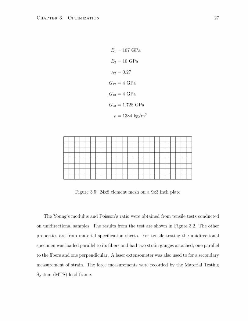
Chapter 3. Optimization 27
E1 = 107 GPa
E2 = 10 GPa
v12 = 0.27
G12 = 4 GPa
G13 = 4 GPa
G23 = 1.728 GPa
ρ = 1384 kg/m3
Figure 3.5: 24x8 element mesh on a 9x3 inch plate
The Young’s modulus and Poisson’s ratio were obtained from tensile tests conducted
on unidirectional samples. The results from the test are shown in Figure 3.2. The other
properties are from material specification sheets. For tensile testing the unidirectional
specimen was loaded parallel to its fibers and had two strain gauges attached; one parallel
to the fibers and one perpendicular. A laser extensometer was also used to for a secondary
measurement of strain. The force measurements were recorded by the Material Testing
System (MTS) load frame.
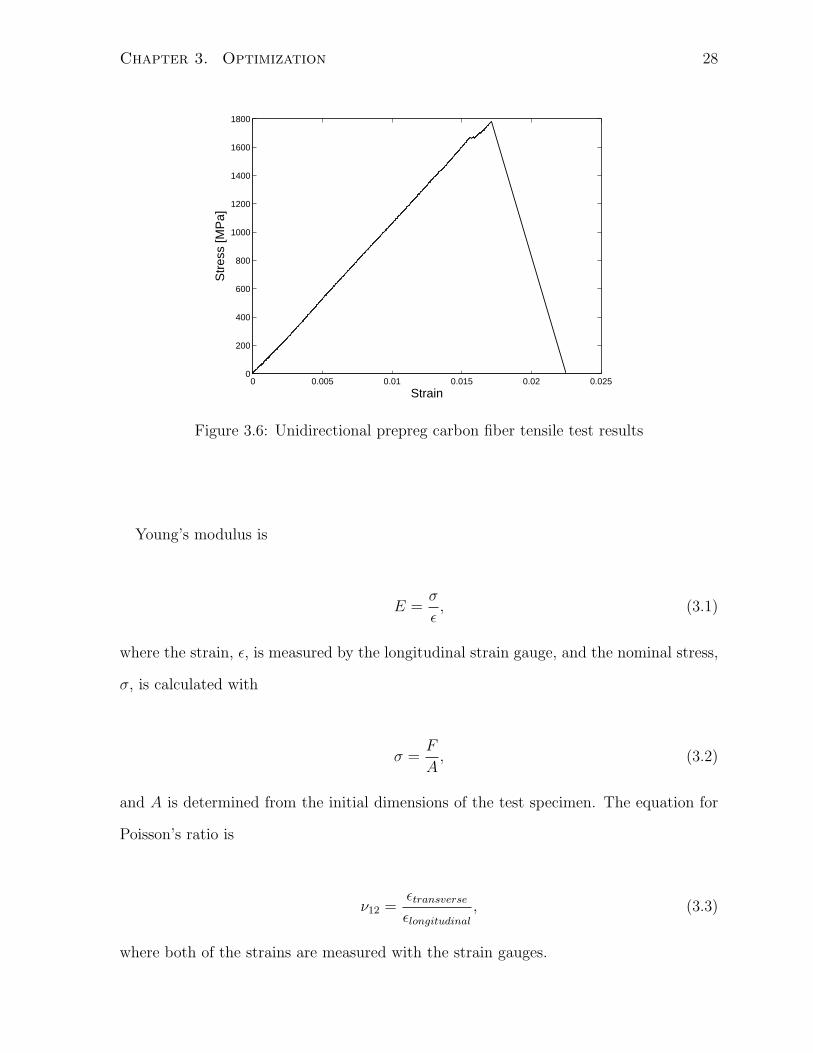
Chapter 3. Optimization 28
0 0.005 0.01 0.015 0.02 0.0250
200
400
600
800
1000
1200
1400
1600
1800
Strain
Str
ess
[MP
a]
Figure 3.6: Unidirectional prepreg carbon fiber tensile test results
Young’s modulus is
E =σ
ǫ, (3.1)
where the strain, ǫ, is measured by the longitudinal strain gauge, and the nominal stress,
σ, is calculated with
σ =F
A, (3.2)
and A is determined from the initial dimensions of the test specimen. The equation for
Poisson’s ratio is
ν12 =ǫtransverseǫlongitudinal
, (3.3)
where both of the strains are measured with the strain gauges.

Chapter 3. Optimization 29
3.2.1 Single Eigenfrequencies
Fiber angles were first optimized for the maximization of single eigenfrequencies to
test the optimization algorithm. Additionally, the results from single eigenfrequency
optimization are more intuitive than the band gap results and therefore it is easier to
anticipate the correct final solution. For both the single eigenfrequency and band gap
optimization a cantilevered boundary condition is used (left side is fixed) and the opti-
mization starts from every fiber angle set to zero, unless stated otherwise. The results
are presented in the form of a figure of the optimized fiber orientations and a plot of the
convergence of the objective function. The ABAQUS verification calculations are also
presented with their respective optimization results. The results for the higher frequen-
cies may also include additional figures for results from higher resolution meshes which
were required to solve accurately for the more complex mode shapes.
The first three odd number eigenfrequencies are predominantly bending modes, and
therefore the optimal fiber orientations for maximizing these eigenfrequencies will be
mostly unidirectional, perpendicular to the cantilevered boundary condition. The mode
shapes can be seen in Figure 3.7. Since the optimal ply for these three modes is unidirec-
tional at 0◦, the initial condition of the plies designated to be optimized was changed to
45◦. Figure 3.8 shows the optimized fiber angles and it can be seen that some fibers did
not end up at 0◦; they remained at 45◦ or somewhere between due to the insensitivity of
of the vibrational response to these fiber angles. Figures 3.9-3.11 show the convergence
of the optimization calculations.
The optimal fiber angles for maximizing these three bending modes all experience
some correlation with each other. The third and fifth modes are strongly correlated to
the first mode due to all three modes being heavily dependent on the fiber angles close
to the cantilevered boundary condition. This can be observed when the fiber angles

Chapter 3. Optimization 30
(a) 1st mode (b) 3rd mode (c) 5th mode
Figure 3.7: Mode shapes for bending eigenfrequencies
(a) 1st mode (b) 3rd mode (c) 5th mode
Figure 3.8: Optimized fiber angles for maximizing the frequencies associated with thefirst three bending modes
are optimized to maximize the 1 − 3 and 1 − 5 gaps. The optimal fiber layout remains
mainly unidirectional and a negligible increase in the bandgap size is produced. On
the other hand, the third and fifth modes are only slightly correlated to each other, as
observed when maximizing the 3 − 5 gap where an increase in approximately 30 Hz is
produced. Section 3.2.3 will provide more details on these arbitrary eigenfrequency gap
maximization results.
The second mode of vibration is the first torsional mode and its optimization follows
the typical convergence profile observed and converges after 19 iterations, as shown in
Figure 3.13. Starting from the second eigenfrequency of the unidirectional plate, which
is approximately 50 Hz, the optimization process converges to a solution with a second

Chapter 3. Optimization 31
0 5 10 15 20 25 30 3512
13
14
15
16
17
18
19
20
21
Iteration
Obj
ectiv
e fu
nctio
n [H
z]
Figure 3.9: Convergence for the maximization of the 1st eigenfrequency from 45◦ start
0 5 10 15 20 25 30 35 4070
80
90
100
110
120
130
140
Iteration
Obj
ectiv
e fu
nctio
n [H
z]
Figure 3.10: Convergence for the maximization of the 3rd eigenfrequency from 45◦ start

Chapter 3. Optimization 32
0 5 10 15 20 25 30220
240
260
280
300
320
340
360
380
Iteration
Obj
ectiv
e fu
nctio
n [H
z]
Figure 3.11: Convergence for the maximization of the 5th eigenfrequency from 45◦ start
eigenfrequency of approximately 85 Hz. The optimized fiber angles are shown in Figure
3.12 along with its mode shape.
The optimization for the maximization of the fourth eigenfrequency follows the same
typical convergence profile as seen previously. The fourth eigenfrequency begins at ap-
proximately 185 Hz and converges to a final eigenfrequency of approximately 272 Hz
after 18 iterations. The fiber angles of the optimized ply are shown in Figure 3.14 along
with the relevant mode shape. The convergence of the optimization process is shown in
Figure 3.15.
The optimization for the maximization of the sixth eigenfrequency starts from approx-
imately 384 Hz and increases to approximately 486 Hz after 15 iterations. The final fiber
angles along with the mode shape of the sixth eigenfrequency are shown in Figure 3.16
and the convergence is plotted in Figure 3.17.

Chapter 3. Optimization 33
(a) Optimized fiber angles (b) Mode shape
Figure 3.12: Comparison of optimized fiber angles to mode shape for the 2nd eigenfre-quency
0 2 4 6 8 10 12 14 16 18 2045
50
55
60
65
70
75
80
85
90
Iteration
Obj
ectiv
e fu
nctio
n [H
z]
Figure 3.13: Convergence for the maximization of the 2nd eigenfrequency
Chapter 3. Optimization 34
(a) Optimized fiber angles (b) Mode shape
Figure 3.14: Comparison of optimized fiber angles to mode shape for the 4th eigenfre-quency
0 2 4 6 8 10 12 14 16 18180
190
200
210
220
230
240
250
260
270
280
Iteration
Obj
ectiv
e fu
nctio
n [H
z]
Figure 3.15: Convergence for the maximization of the 4th eigenfrequency

Chapter 3. Optimization 35
(a) Optimized fiber angles (b) Mode shape
Figure 3.16: Comparison of optimized fiber angles to mode shape for the 6th eigenfre-quency
0 5 10 15380
400
420
440
460
480
500
Iteration
Obj
ectiv
e fu
nctio
n [H
z]
Figure 3.17: Convergence for the maximization of the 6th eigenfrequency

Chapter 3. Optimization 36
As the mode number increases the complexity of the mode shapes increases. At a
certain point the resulting optimized fiber angles become too complex to lay-up by hand
and the eigenfrequecy becomes too difficult to measure with modal testing. With an
increase in mode shape complexity the optimization process will have to use a higher
resolution mesh as well, which will greatly increase the computational time required.
Therefore the optimization process was only used up to the sixth mode of vibration.
3.2.2 Eigenfrequency Bandgaps
This section presents the results of the band gap optimization calculations, which
is the main objective of this thesis. The results are presented in the format used in
the previous section with the addition of comparisons to related single eigenfrequency
optimization results. Beginning with the first band gap, which is the distance between
the first and second eigenfrequencies, the optimized fiber angles are shown in Figure 3.18
and they are almost identical to the optimized fiber angles for the maximization of the
second eigenfrequency. The bandgap begins the optimization at approximately 29 Hz
(unidirectional plate) and increases to approximately 72 Hz after 20 iterations, as shown
in Figure 3.19.
Figure 3.18: Results of optimization for maximization of the bandgap between the 1st
and 2nd eigenfrequencies

Chapter 3. Optimization 37
0 2 4 6 8 10 12 14 16 18 2025
30
35
40
45
50
55
60
65
70
75
Iteration
Obj
ectiv
e fu
nctio
n [H
z]
Figure 3.19: Convergence for the maximization of the bandgap between the 1st and 2nd
eigenfrequencies
Modes
Description 1 2 3 4 5 6
Optimized 13.66 85.71 90.16 290.85 262.38 428.71
ABAQUS 14.20 85.23 91.90 240.39 269.12 429.19
Table 3.1: Eigenfrequencies calculated from optimized results from maximization of the1st and 2nd eigenfrequencies
Table 3.1 presents the eigenfrequencies calculated with both the opimized results and
the ABAQUS approximation of the results. The differences between the values calculated
for each mode are minimal except for the fourth mode where there is an approxiately
50 Hz difference. The cause of this large discrepancy could be attributed to the ap-
proximations made to the optimized results to aid in modeling the layup in ABAQUS.
During the modeling the fibre angles were rounded to the nearest multiple of 5 and some
fiber angles were also adjusted for symmetry. These adjustments would have the largest

Chapter 3. Optimization 38
impact on the center of the plate where the fibers switch direction. This area has some
fibers with angles that don’t seem to follow the pattern observed in the rest of the plate;
coincidentally, this area is also near an inflection point in the fourth mode shape, so a
change to the fiber angles in this area could affect the performance of the plate with
respect to the fourth mode.
When optimizing for the maximization of the bandgap between the second and third
eigenfrequencies it was found that the optimized fiber angles do not differ much from the
unidirectional starting condition, as can be seen in Figure 3.20. With minimal change
in the fiber angles there will be minimal change in the vibrational characteristics of the
composite plate, which can be seen in the convergence plot Figure 3.21. The optimization
procedure required only 8 iterations and the bandgap only increased by approximately 2
Hz. In Table 3.2 the eigenfrequencies of the optimized plate are compared to the results
of calculations performed in ABAQUS on a 5 ply unidirectional plate (optimized lay-up
is assumed to be unidirectional). The eigenfrequencies from the two sources are very
similar and only diverge slightly as the mode number increases.
Figure 3.20: Results of optimization for maximization of the bandgap between the 2nd
and 3rd eigenfrequencies

Chapter 3. Optimization 39
0 1 2 3 4 5 6 780.5
81
81.5
82
82.5
83
Iteration
Obj
ectiv
e fu
nctio
n [H
z]
Figure 3.21: Convergence for the maximization of the bandgap between the 2nd and 3rd
eigenfrequencies
Modes
Description 1 2 3 4 5 6
Optimized 20.30 46.75 129.60 187.34 359.35 387.25
ABAQUS 20.72 49.72 129.98 183.73 363.35 379.47
Table 3.2: Eigenfrequencies calculated from optimized results from maximization of the2nd and 3rd eigenfrequencies
The optimized fiber angles for the maximization of the bandgap between the 3rd and
4th are the same as the 4th eigenfrequency maximization results. Figure 3.22 shows
the optimized fiber angles and Figure 3.23 shows the convergence of this optimization
process. The objective function begins at approximately 54 Hz and converges to about
170 Hz, over three times larger than the starting unidirectional bandgap. Table 3.3
presents the comparison between the optimization results and the ABAQUS results from
the approximated optimized lay-up.

Chapter 3. Optimization 40
Figure 3.22: Results of optimization for maximization of the bandgap between the 3rd
and 4th eigenfrequencies
0 2 4 6 8 10 1240
60
80
100
120
140
160
180
Iteration
Obj
ectiv
e fu
nctio
n [H
z]
Figure 3.23: Convergence for the maximization of the bandgap between the 3rd and 4th
eigenfrequencies
Modes
Description 1 2 3 4 5 6
Optimized 15.54 63.88 94.33 265.41 266.68 435.15
ABAQUS 15.69 62.80 101.43 271.27 273.06 440.19
Table 3.3: Eigenfrequencies calculated from optimized results from maximization of the3rd and 4th eigenfrequencies

Chapter 3. Optimization 41
The results of the optimization for the maximization of the bandgap between the 4th
and 5th eigenfrequencies are shown in Figures 3.24 and 3.25. In a similar manner to
the 2 − 3 bandgap optimization, the optimized fiber angles are largely unidirectional
at 0◦. It can be seen on the convergence plot that the objective function increases from
approximately 182 Hz to 205 Hz over 20 iterations. Table 3.4 presents the eigenfrequencies
of the optimized plate as calculated from the optimization results and from the ABAQUS
approximation and it can be seen that there are some noticeable differences between the
results for the second, third and fifth modes. Like the discrepancy mentioned previously
for the 1− 2 bandgap plate, the cause of these differences can also be attributed to the
approximation process. The optimal ply for the 5− 6 bandgap maximization is the most
complex of the results presented in this thesis and therefore the approximation process
will have a larger affect on its eigenfrequencies than it would on the more basic optimal
plies.
Figure 3.24: Results of optimization for maximization of the bandgap between the 4th
and 5th eigenfrequencies

Chapter 3. Optimization 42
0 2 4 6 8 10 12 14 16 18 20180
185
190
195
200
205
210
Iteration
Obj
ectiv
e fu
nctio
n [H
z]
Figure 3.25: Convergence for the maximization of the bandgap between the 4th and 5th
eigenfrequencies
Modes
Description 1 2 3 4 5 6
Optimized 19.28 50.77 114.58 157.87 363.02 384.56
ABAQUS 19.42 49.98 114.95 158.50 360.29 384.91
Table 3.4: Eigenfrequencies calculated from optimized results from maximization of the4th and 5th eigenfrequencies
The maximization of the 5− 6 bandgap begins at approximately 18 Hz and increases
to around 224 Hz after 21 iterations. The optimized fiber angles are shown in Figure 3.26
and the convergence of the objective function can be seen in Figure 3.26. The comparison
of the optimization results and the ABAQUS approximation is presented in Table 3.5.
Comparing these results with the previous few sets it is clear that the optimal fiber angles
for maximizing the 5 − 6 bandgap are more complex. This can also be observed in the
ABAQUS calculations which show a larger difference from the optimization results than

Chapter 3. Optimization 43
the other bandgap optimizations.
Figure 3.26: Results of optimization for maximization of the bandgap between the 5th
and 6th eigenfrequencies
0 2 4 6 8 10 12 14 16 18 20 220
50
100
150
200
250
Iteration
Obj
ectiv
e fu
nctio
n [H
z]
Figure 3.27: Convergence for the maximization of the bandgap between the 5th and 6th
eigenfrequencies
Modes
Description 1 2 3 4 5 6
Optimized 16.15 69.72 97.85 225.12 261.38 484.86
ABAQUS 17.80 58.34 110.16 226.13 300.71 484.25
Table 3.5: Natural frequencies [Hz] calculated for the optimal fiber angles for the maxi-mization of the bandgap between the 5th and 6th eigenfrequencies

Chapter 3. Optimization 44
3.2.3 Other Eigenfrequency Gaps
In addition to the single eigenfrequency and bandgap optimization, the fiber angles
were optimized to maximize the gap between arbitrary eigenfrequencies for informational
purposes. Presented below are the resulting optimized fiber angles and the plots of their
convergence.
The gap between the first and third eigenfrequencies does not change much through-
out the optimzation process, as shown in Figure 3.28. This is due to the fact that the
maximized fiber angles for the single eigenfrequencies are nearly identical (fully unidirec-
tional).
The resulting optimized fiber angles for the 1 − 4 and 2 − 4 gaps are nearly identical
to each other and to the results from the 3 − 4 bandgap and the fourth eigenfrequency
maximization. The results from the 1− 4 gap optimization are shown in Figure 3.29 and
the 2 − 4 gap results are in Figure 3.30. Both sets of results show a large improvement
over the unidirectional starting condition.
The results from the optimization for the first two gaps, 1−5 and 2−5, show minimal
improvement from the unidirectional starting condition. However, the maximization of
the 3− 5 gap shows some improvement increasing from approximately 236 Hz to 264 Hz
over 32 iterations. The results for these optimizations are presented in Figures 3.31 -
3.33.
Unlike the previous sets of optimizations, the results for maximizing gaps using the
sixth eigenfrequency provide several unique ply designs. The results for the maximiza-
tion of the 1 − 6 gap are shown in Figure 3.34. The objective function increases from
approximately 365 Hz to 495 Hz following an atypical convergence path. Figure 3.35
presents the outcome of maximizing the 2 − 6 gap. It went from approximately 335 Hz

Chapter 3. Optimization 45
(a) Optimized fiber angles
0 5 10 15 20 25 30 35 40 45109.5
110
110.5
111
111.5
112
112.5
113
113.5
Iteration
Obj
ectiv
e fu
nctio
n [H
z]
(b) Convergence
Figure 3.28: Optimization results for the maximization of the 1− 3 gap
(a) Optimized fiber angles
0 2 4 6 8 10 12 14 16160
170
180
190
200
210
220
230
240
250
260
Iteration
Obj
ectiv
e fu
nctio
n [H
z]
(b) Convergence
Figure 3.29: Optimization results for the maximization of the 1− 4 gap

Chapter 3. Optimization 46
(a) Optimized fiber angles
0 2 4 6 8 10 12 14 16 18130
140
150
160
170
180
190
200
210
220
Iteration
Obj
ectiv
e fu
nctio
n [H
z]
(b) Convergence
Figure 3.30: Optimization results for the maximization of the 2− 4 gap
(a) Optimized fiber angles
0 1 2 3 4 5
345.4
345.6
345.8
346
346.2
346.4
346.6
346.8
347
347.2
Iteration
Obj
ectiv
e fu
nctio
n [H
z]
(b) Convergence
Figure 3.31: Optimization results for the maximization of the 1− 5 gap

Chapter 3. Optimization 47
(a) Optimized fiber angles
0 1 2 3 4 5 6 7 8 9316
316.5
317
317.5
318
318.5
319
Iteration
Obj
ectiv
e fu
nctio
n [H
z]
(b) Convergence
Figure 3.32: Optimization results for the maximization of the 2− 5 gap
(a) Optimized fiber angles
0 5 10 15 20 25 30 35235
240
245
250
255
260
265
Iteration
Obj
ectiv
e fu
nctio
n [H
z]
(b) Convergence
Figure 3.33: Optimization results for the maximization of the 3− 5 gap

Chapter 3. Optimization 48
to 390 Hz.
The optimized fiber angles for the 3 − 6 gap, seen in Figure 3.36, are similar to the
results from the 1− 6 gap maximization. The objective function starts at approximately
255 Hz and increases to about 410 Hz after 22 iterations. The results for the 4 − 6 gap
optimization are shown in Figure 3.37. Its objective function increases by 60 Hz in 29
iterations, starting from around 200 Hz.

Chapter 3. Optimization 49
(a) Optimized fiber angles
0 10 20 30 40 50 60360
380
400
420
440
460
480
500
Iteration
Obj
ectiv
e fu
nctio
n [H
z]
(b) Convergence
Figure 3.34: Optimization results for the maximization of the 1− 6 gap
(a) Optimized fiber angles
0 2 4 6 8 10 12 14330
340
350
360
370
380
390
400
Iteration
Obj
ectiv
e fu
nctio
n [H
z]
(b) Convergence
Figure 3.35: Optimization results for the maximization of the 2− 6 bandgap

Chapter 3. Optimization 50
(a) Optimized fiber angles
0 5 10 15 20 25240
260
280
300
320
340
360
380
400
420
Iteration
Obj
ectiv
e fu
nctio
n [H
z]
(b) Convergence
Figure 3.36: Optimization results for the maximization of the 3− 6 bandgap
(a) Optimized fiber angles
0 5 10 15 20 25 30190
200
210
220
230
240
250
260
270
Iteration
Obj
ectiv
e fu
nctio
n [H
z]
(b) Convergence
Figure 3.37: Optimization results for the maximization of the 4− 6 bandgap

Chapter 4
Modal Analysis
To validate the results presented in the previous chapter, the optimized laminated com-
posite plates were fabricated from unidirectional prepreg carbon fiber tape and subjected
to modal testing. In conjunction with the modal testing, commercial FEA software was
used to determine the vibrational characteristics of the optimized plates, and to also
ensure that there were no errors in the optimization results before plate fabrication had
begun. This chapter presents the results of the modal analysis of the plates along with
an overview of the fabrication and testing procedures used.
4.1 Testing Procedure
As mentioned previously in Chapter 2, the hardware used in the modal testing is an
impact hammer for excitation and an accelerometer for measuring the response. Both
were purchased from PCB Piezotronics Inc; the hammer is model 086C01 and the ac-
celerometer is model 352A24. The accelerometer and impact hammer are shown in Figure
4.2. The data aquisition and signal conditioning were performed with a National Instru-
ments signal conditioner, SC-2354, with two SCC-ACC01 Accelerometer input modules,
connected to a computer with Labview software. The Labview interface created for the
modal analysis samples the inputs from the input modules at a user specified sampling
51

Chapter 4. Modal Analysis 52
(a) Accelerometer (b) Impact Hammer
Figure 4.2: Modal testing hardware shown with a pencil for scale
frequency and writes the values to a spreadsheet. These are the time-domain values
which are analyzed as stated in Chapter 2. The Labview block diagram is shown in
Figure 4.1.
Figure 4.1: Labview block diagram for reading modal analysis data and saving to a file
The general procedure for performing the modal testing is straightforward. The ac-
celerometer is attached to a specific point on the plate with wax and the impact hammer
is used to provide an impulse at a certain location, and ten measurements are taken to
ensure high quality data is recorded and to allow for the averaging of results. The location
of the accelerometer and hammer strikes were rotated through several different locations

Chapter 4. Modal Analysis 53
in an effort to capture all relevant modes of vibration. To impose the cantilevered bound-
ary condition one end of the plate is clamped in a table clamp. A cantilevered plate with
accelerometer attached can be seen in Figure 4.3.
Figure 4.3: Accelerometer attached to plate ready for testing
4.2 Fabrication
To lay up the optimized plies by hand the optimization results have to be converted to
a simpler design while still maintaining the vibrational characteristics of the optimized
results. This is accomplished by grouping fiber angles with similar surrounding fibers to
produce larger unidirectional ”patches”. An example of a plate constructed from these
unidirectional patches can be seen in Figure 4.4.
Chapter 4. Modal Analysis 54
Figure 4.4: Lay-up of an optimized ply for the maximization of the 2nd eigenfrequency
The plates were first made with the same 5-ply lay-up configuration as used for the
optimization process, [opt, 0◦, ¯opt]s, where ”opt” refers to a ply composed of the optimal
local fiber angles, but a problem was encountered when the plates warped during the
curing process. Due to the orthotropic properties of the material and the optimized
plies, certain areas of the plate will contract more than the others upon curing, creating
a warp in the plate and thus preventing it from undergoing modal testing. Several
potential solutions were attempted, such as modifying the lay-up configurations to [opt,
0◦, 0̄◦]s or [opt, 0◦, ¯90◦]s and using a heavy flat plate on top of the bagged plate during
curing. Unfortunately none of these solutions were able to entirely remove the warping,
so additional plies had to be added to increase the thickness of the plate. The following
10-ply lay-up configuration was used for the modal testing: [opt, 0◦, opt, 90◦, 0̄◦]s. By
doubling the number of plies, the warping was eliminated.
4.3 Results
In this section the results from the modal testing are presented along with ABAQUS
calculations for the 10-ply plates. Calculations were performed in ABAQUS uing two dif-

Chapter 4. Modal Analysis 55
ferent versions of the optimized ply; one being the regular optimization results (corrected
for symmetry and angles rounded to nearest multiple of five) and the other being the ap-
proximated hand lay-up version on which the plate fabrication was based on. The results
of the modal testing are presented as plots of the frequency response function measured
at two different locations: the top-center and top-right corner of the cantilevered plate.
Additionally, the eigenfrequencies as calculated by ABAQUS for the approximated lay-
up version of the plate are plotted as vertical lines over the FRF plot to allow for an easy
comparison of experimental and theoretical results.
The results of the modal testing of the plate optimized for the maximization of the
1 − 2 bandgap are presented in Figures 4.5 and 4.6. From both figures it can be seen
that the first three eigenfrequencies in the frequency response function (FRF) match
their respective predicted values which are presented in Table 4.1. As the mode number
increases, some divergence is seen in the predicted and experimental eigenfrequencies.
The fourth and fifth predicted eigenfrequencies fall on either side of a peak in the FRF
and the sixth eigenfrequency of the FRF was found to be either slightly lower or higher
than the predicted value based on the placement of the accelerometer.
0 100 200 300 400 500 600 700 800 900 1000−80
−70
−60
−50
−40
−30
−20
−10
0
10
20
Frequency [Hz]
Am
plitu
de [d
B]
ExperimentalPredicted
Matching frequencies
Figure 4.5: Frequency response funtion calculated from the accelerometer attached tothe top-center of the plate with a maximized 1− 2 bandgap

Chapter 4. Modal Analysis 56
0 100 200 300 400 500 600 700 800 900 1000−70
−60
−50
−40
−30
−20
−10
0
10
20
Frequency [Hz]
Am
plitu
de [d
B]
ExperimentalPredicted
Matching frequencies
Figure 4.6: Frequency response funtion calculated from the accelerometer attached tothe top-right corner of the plate with a maximized 1− 2 bandgap
Modes
Description 1 2 3 4 5 6
Optimized 31.02 164.75 194.86 474.46 564.31 910.59
Layup 29.70 161.51 185.23 466.31 542.24 891.67
Table 4.1: Predicted results from ABAQUS calculations for the 1−2 bandgap maximiza-tion
The experimental results of the 2 − 3 bandgap plate show little correlation with the
predicted eigenfrequencies. One possible reason is the fact that the optimized ply is fully
unidirectional with the fibers all oriented at 0◦ from horizontal; this creates an incredibly
stiff plate in bending and therefore the amplitude and the length of the induced vibrations
are very small. The first three predicted eigenfrequencies are close to peaks of the FRF
in Figure 4.7. The first and third eigenfrequencies match up well with a small and large
peak, respectively, on both FRF plots, while the predicted second eigenfrequency lies
between two small peaks in Figure 4.7. The remaining sets of eigenfrequencies do not
match up at all. Since the optimized ply was very similar to a unidirectional ply, the
eigenfrequencies were calculated for the lay-up only. The predicted eigenfrequencies can

Chapter 4. Modal Analysis 57
be found in Table 4.2.
0 100 200 300 400 500 600 700 800 900 1000−60
−50
−40
−30
−20
−10
0
10
20
30
Frequency [Hz]
Am
plitu
de [d
B]
ExperimentalPredicted
Matching frequencies
Figure 4.7: Frequency response funtion calculated from the accelerometer attached tothe top-center of the plate with a maximized 2− 3 bandgap
0 100 200 300 400 500 600 700 800 900 1000−80
−70
−60
−50
−40
−30
−20
−10
0
10
20
Frequency [Hz]
Am
plitu
de [d
B]
ExperimentalPredictedMatching frequencies
Figure 4.8: Frequency response funtion calculated from the accelerometer attached tothe top-right corner of the plate with a maximized 2− 3 bandgap
Modes
Description 1 2 3 4 5 6
Layup 40.39 98.44 252.91 361.48 707.93 814.52
Table 4.2: Predicted results from ABAQUS calculations for the 2−3 bandgap maximiza-tion

Chapter 4. Modal Analysis 58
The testing results of the plate optimized for the maximization of the bandgap between
the third and fourth eigenfrequencies are shown in Figures 4.9 and 4.10. The predicted
first, third and sixth eigenfrequencies correspond well to the experimental data, each
on (or very near) a peak in at least one of the FRFs. The fourth and fifth predicted
eigenfrequencies fall on either side of a wide peak in Figure 4.9, while no peak in the
FRF is present for the second eigenfrequency. The calculated eigenfrequencies are shown
in Table 4.3.
0 100 200 300 400 500 600 700 800 900 1000−80
−70
−60
−50
−40
−30
−20
−10
0
10
20
Frequency [Hz]
Am
plitu
de [d
B]
ExperimentalPredictedMatching frequencies
Figure 4.9: Frequency response funtion calculated from the accelerometer attached tothe top-center of the plate with a maximized 3− 4 bandgap
0 100 200 300 400 500 600 700 800 900 1000−70
−60
−50
−40
−30
−20
−10
0
10
20Frequency Response Function
Frequency [Hz]
Am
plitu
de [d
B]
ExperimentalPredicted
Matching frequencies
Figure 4.10: Frequency response funtion calculated from the accelerometer attached tothe top-right corner of the plate with a maximized 3− 4 bandgap

Chapter 4. Modal Analysis 59
Modes
Description 1 2 3 4 5 6
Optimized 33.16 124.85 213.93 523.61 579.20 879.99
Layup 33.04 131.85 206.12 513.54 567.05 868.37
Table 4.3: Predicted results from ABAQUS calculations for the 3−4 bandgap maximiza-tion
Figures 4.11 and 4.12 show the test results for the 4 − 5 bandgap optimized plate.
As with the previous plate, the first, third, and sixth predicted eigenfrequencies match
up well with their experimental values and the predicted second eigenfrequency does not
correspond to any peak on the FRF. With the accelerometer placed in the top-right corner
of the plate a peak which is near the predicted fourth eigenfrequency appears in the FRF.
In addition, Figure 4.11 has peak in the FRF in the vicinity of the fifth eigenfrequency,
demonstrating that accelerometer placement has an effect on the observed frequencies.
The calculated eigenfrequencies are presented in Table 4.4.
0 100 200 300 400 500 600 700 800 900 1000−80
−70
−60
−50
−40
−30
−20
−10
0
10
20
Frequency [Hz]
Am
plitu
de [d
B]
ExperimentalPredictedMatching frequencies
Figure 4.11: Frequency response funtion calculated from the accelerometer attached tothe top-center of the plate with a maximized 4− 5 bandgap

Chapter 4. Modal Analysis 60
0 100 200 300 400 500 600 700 800 900 1000−90
−80
−70
−60
−50
−40
−30
−20
−10
0
10
20
Frequency [Hz]
Am
plitu
de [d
B]
ExperimentalPredictedMatching frequencies
Figure 4.12: Frequency response funtion calculated from the accelerometer attached tothe top-center of the plate with a maximized 4− 5 bandgap
Modes
Description 1 2 3 4 5 6
Optimized 38.54 100.37 232.43 323.80 702.84 846.53
Layup 38.58 103.49 230.42 324.49 692.87 847.93
Table 4.4: Predicted results from ABAQUS calculations for the 4−5 bandgap maximiza-tion
The final plate tested was the one optimized for the maximization of the 5−6 bandgap.
The results are presented in Figures 4.13 and 4.14. The first and third predicted eigenfre-
quencies match up well with peaks in the FRF in both plots, but, like previouisly, there
is no peak in the FRF near the second eigenfrequency. When the accelerometer is placed
at the top-center of the plate the fourth and fifth eigenfrequencies are on either side of a
peak in the FRF; with the accelerometer placed in the top-right corner the peak in the
FRF moves to a frequency slightly higher than the predicted fifth frequency. Looking
at the sixth eigenfrequency, the predicted value is slightly higher in frequency than the
peak in the FRF, with the FRF in Figure 4.14 being closer to the predicted than the
FRF in Figure 4.13. The calculated eigenfrequencies are located in Table 4.5.

Chapter 4. Modal Analysis 61
0 100 200 300 400 500 600 700 800 900 1000−80
−70
−60
−50
−40
−30
−20
−10
0
10
20
Frequency [Hz]
Am
plitu
de [d
B]
ExperimentalPredictedMatching frequencies
Figure 4.13: Frequency response funtion calculated from the accelerometer attached tothe top-center of the plate with a maximized 5− 6 bandgap
0 100 200 300 400 500 600 700 800 900 1000−90
−80
−70
−60
−50
−40
−30
−20
−10
0
10
20
Frequency [Hz]
Am
plitu
de [d
B]
ExperimentalPredicted
Matching frequencies
Figure 4.14: Frequency response funtion calculated from the accelerometer attached tothe top-right corner of the plate with a maximized 5− 6 bandgap
Modes
Description 1 2 3 4 5 6
Optimized 33.28 138.94 204.88 447.96 562.19 958.80
Layup 31.87 136.96 200.98 423.12 557.10 959.11
Table 4.5: Predicted results from ABAQUS calculations for the 5−6 bandgap maximiza-tion

Chapter 4. Modal Analysis 62
Overall, the frequency response functions aligned with around half of the predicted
eigenfrequencies while also sometimes having peaks near the other predicted values. It
was also noticed that for the majority of the optimized plates the second predicted
eigenfrequency did not line up with the observed results. When this was the case the
FRF would have a peak in between the first and second eigenfrequencies. A possible
cause for this could be the placement of the accelerometer; its current locations may not
have been in a region with a large amount of amplitude. Another interesting observation
is that the bandgaps which were the focus of the observation are easily visible when
viewing the plotted predicted eigenfrequencies. While all of the bandgaps vary in size,
the maximized one is clearly the largest and easily spotted.

Chapter 5
Conclusions
This thesis presents a method for optimizing the local fiber orientations in thin com-
posite plates to maximize specific eigenfrequencies and eigenfrequency bandgaps. This
optimization process can be useful when confronted with the need to maximize the per-
formance of a geometrically constrained composite component. The orthotropic nature
of the mechanical properties of carbon fiber are taken advantage of to produce a part
using the most efficient use of material possible.
The composite plates were modelled using First Order Shear Deformation Theory
which assumes the laminated plate is a single layer with complex constitutive behaviour.
When the plates are discretized, each element will have a set of fiber angles correspond-
ing to each ply. Prior to the optimization process it has to be dedcided which plies
to optimize. The Steepest Descent Method was used to conduct the optimization, the
sensitivities were calculated using a simple finite difference approximation, and the opti-
mal step size was determined using the golden section search method. The optimization
process was performed on cantilevered rectangular plates which had an aspect ratio of
3:1.
63

Chapter 5. Conclusions 64
In the single eigenfrequency maximization case, it was shown that the optimization
process will provide a significant increase in the targeted eigenfrequency over the uni-
directional starting condition. In addition, viewing the optimized fiber angles and the
vibration mode shape next to each other allows for a greater understanding of their re-
lationship. When maximizing eigenfrequency bandgaps the optimal fiber orientations
are often very similar to the results from the single eigenfrequency maximization for the
larger eigenfrequency in the bandgap (i.e. the results from the 1 − 2 bandgap maxi-
mization are the same as the results from the 2nd eigenfrequency maximization). As the
mode numbers of the bandgap increase, the similarity between the bandgap and single
eigenfrequency maximization results is reduced; this begins for the 4− 5 eigenfrequency
bandgap. Generally, a large increase in the targeted bandgap was observed during the
optimization process. The exception to this were the 2− 3 and 4− 5 bandgaps and the
other arbitrary gaps with 3 or 5 as the larger of the two frequencies. Since these gaps
and bandgaps had an odd eigenfrequency as the dominant frequency of the pair their
optimal fiber orientations are heavily unidirectional which is the starting condition.
To validate the results from the optimization process the optimal fiber orientations
were converted into an approximate lay-up and 10-ply laminated composite plates, [opt,
0◦, opt, 90◦, 0̄◦]s, were fabricated for modal testing. The modal testing was conducted
using an accelerometer, attached to the plate with wax, and an impact hammer, to
provide excitation. The instrumentation was controlled with Labview and the data was
analyzed in Matlab.
The results of the modal testing can be found in Section 4.3. The vibration was
recorded at the top-center and top-right corners of the plates. One observation from
the figures of the results is that the higher eigenfrequencies are both more difficult to
measure and more difficult to control. The FRF plots rarely had any prominent peaks
for the fourth and fifth eigenfrequencies while the sixth eigenfrequency sometimes had

Chapter 5. Conclusions 65
a peak (which may or may not have been near the predicted sixth eigenfrequency). On
the other hand the first and third eigenfrequencies ususally had the predicted values
near the experimental results. The second eigenfrequency had more unique results; there
was always a prominent peak in the FRF plot but it was usually not near the predicted
value. Only the results from the 1−2 bandgap have matching predicted and experimental
second eigenfrequencies.
The optimization results presented in Secton 3 demonstrated the feasibility of opti-
mizing the orientation of orthotropic material for the maximization of eigenfrequency
bangaps. The results in this section were also verified with commercial FEA software.
Fabricating the optimized plates and subjecing them to modal testing demonstrated that
the increased bandgap size does carry over from the theoretical calculations. A great ex-
ample of this are the 1− 2 bandgap maximization results. However, it was also observed
that as the mode numbers increase so does the difficulty of fabricating the optimized fiber
layout, and therefore it is more difficult to maintain the predicted vibrational character-
istics. A more accurate method of fabrication may be required for the more complicated
optimized designs, which will be discussed in more detail in the next section, along with
other recommendations.
5.1 Recommendations
There are several ways in which the optimization process can be improved. The change
to the optimization algorithm that will yield the greatest results in terms of efficiency is to
use the adjoint method to calculate the sensitivities in place of the current finite difference
method, as seen in [13] and [6]. With the adjoint method, the eigenvalues do not need to
be recalculated for every design variable (fiber angle); instead only the stiffness matrix
needs to be recalculated and this is a much quicker process. Another improvement in the
calculation speed can be made by using an algorithm that is more suitable for solving

Chapter 5. Conclusions 66
the general eigenproblem with large symmetric positive definite matrices. Currently
QR decomposition is used, but using an algorithm such as the Lanczos method or sub-
space iteration should improve the calculaton speed [4]. A quicker eigenproblem solving
algorithm will have a large impact on the speed of the step size line search portion of
the optimizaion process since the eigenvalues need to be calculated in every iteration
of the line search. Lastly, the optimization algorithm itself should be considered for
improvement. Currently the steepest descent method is used; it is simple but slow. One
option would be to use the Method of Moving Asymptotes (MMA) as described by [20]
and [21], and used in [13] and [5] among others. More efficient optimization methods
can reduce the number of iterations required before a convergence to a solution and also
decrease the time required per iteration.
One aspect of composite design that was not considered in the optimization process is
manufacturability. The fiber angles of adjacent elements are unrestricted and therefore
the optimized designs could create some difficulties in their fabrication, even when using
technologies such as advanced tow placement. To incorporate manufacturability into
the optimization process one could impose constraints on fiber angles to ensure that the
results are viable or possibly employ some form of post-processing on the results to create
a manufacturable final product.
To get optimized results that are more forgiving for hand lay-up a different approach
may have to be taken. Discrete material optimization (DMO) is a method that is very
similar topology optimization with multiple materials. In the place of the multiple dif-
ferent materials that topology optimization would use, DMO will have an orthotropic
material defined at many different angles (i.e. 0◦,±15◦,±30◦, etc). DMO also employs
the Solid Isotropic Material with Penalization (SIMP) approach and can be solved using
MMA [19][7]. In addition to the fixed angles which make the hand lay-up process simpler,
DMO can also use patch variables to group many elements together to act as one, which

Chapter 5. Conclusions 67
resemble patches of unidirectional prepreg tape.

Bibliography
[1] Gnu scientific library. http://www.gnu.org/software/gsl/.
[2] Open mpi. http://www.open-mpi.org/.
[3] Openmp. http://openmp.org/wp/.
[4] K. Bathe. Finite Element Procedures in Engineering Analysis. Prentice-Hall, Inc.,
1982.
[5] A. Larsen et al. Topological material layout in plates for vibration suppression and
wave propagation control. Structural and Multidisciplinary Optimization, 37:585–
594, 2009.
[6] A. P. Seyranian et al. Multiple eigenvalues in structural optimization problems.
Structural and Multidisciplinary Optimization, 8:207–227, 1994.
[7] B. Niu et al. Discrete material optimization of vibrating laminated composite
plates for minimum sound radiation. International Journal of Solids and Structures,
47:2097–2114, 2010.
[8] D. Ewins. Modal Testing. Research Studies Press, 2000.
[9] A. J. M. Ferreira. MATLAB Codes for Finite Element Analysis. Springer, 2009.
68
Bibliography 69
[10] Du Jianbin and Niels Olhoff. Topological design of freely vibrating continuum struc-
tures for maximum values of simple and multiple eigenfrequencies and frequency
band gaps. Structural and Multidisciplinary Optimization, 34:91–110, 2007.
[11] R. Jones. Mechanics of Composite Materials. Taylor and Francis, 1999.
[12] N. L. Pedersen. Maximization of eigenvalues using topology optimiaztion. Structural
and Multidisciplinary Optimization, 20:2–11, 2000.
[13] N. L. Pedersen. Designing plates for minimum internal resonances. Structural and
Multidisciplinary Optimization, 30:297–307, 2005.
[14] J. N. Reddy. Mechanics of Laminated Composite Plates and Shells, Theory and
Analysis. CRC Press, 2004.
[15] O. Sigmund. A 99 line topology optimization code written in matlab. Structural
and Multidisciplinary Optimization, 21:120–127, 2001.
[16] O. Sigmund and S. Torquato. Design of materials with extreme elastic or thermoelas-
tic properties using topology optimization. IUTAM Symposium on Transformation
Problems in Composite and Active Materials, pages 233–244, 1998.
[17] O. Sigmund and S. Torquato. Design of smart composite materials using topology
optimization. Smart Materials and Structures, 8:365–379, 1998.
[18] Ole Sigmund. On the design of compliant mechanisms using topology optimization.
Mechanics Based Design of Structures and Machines, 25:493–524, 1997.
[19] J. Stegmann and E. Lund. Discrete material optimization of general composite shell
structures. International Journal for Numerical Methods in Engineering, 62:2009–
2027, 2005.

Bibliography 70
[20] K. Svanberg. The method of moving asymptotes - a new method for structural
optimization. International Journal for Numerical Methods in Engineering, 24:359–
373, 1987.
[21] C. Zillober. A globally convergent version of the method of moving asymptotes.
Structural and Multidisciplinary Optimization, 6:166–174, 1993.