Fourth Order Compact Finite Volume Scheme on Nonuniform Grids With Multi-blockin

Computers & Fluids 56 (2012) 1–16

Contents lists available at SciVerse ScienceDirect

Computers & Fluids

journal homepage: www.elsevier .com/ locate /compfluid

Fourth order compact finite volume scheme on nonuniform gridswith multi-blocking

M. Ghadimi, M. Farshchi ⇑Aerospace Engineering Department, Sharif University of Technology, Azadi Av., Tehran, Iran

a r t i c l e i n f o

Article history:Received 12 August 2010Received in revised form 11 July 2011Accepted 16 November 2011Available online 7 December 2011

Keywords:Fourth orderCompact schemeFinite volumeNonuniform gridsMulti-block domain

0045-7930/$ - see front matter � 2011 Elsevier Ltd. Adoi:10.1016/j.compfluid.2011.11.007

⇑ Corresponding author. Tel.: +98 21 66164605; faxE-mail address: [email protected] (M. Farshchi).

a b s t r a c t

We have developed a fourth order compact finite volume method for the solution of low Mach numbercompressible flow equations on arbitrary nonuniform grids. The formulation presented here uses collo-cated grid that preserves fourth order accuracy on nonuniform meshes. This was achieved by introduc-tion of a new fourth order method for calculation of cell and face averaged metrics. A special treatment ofnonlinear terms is used to guarantee the stability of the fourth order compact method. Moreover anapproach for applying this method to multi-block domains is presented for complicated geometriesand parallel processing applications. Several test cases including the flow in a lid-driven cavity, laminarflow over a flat plate, decay of the Taylor vortex, and transient flow behind a backward facing step showthe accuracy, efficiency, and stability of the method in single and multi-block domains. To the best of ourknowledge, this is the first symmetric compact method in the finite volume form that can achieve fullfourth order accuracy in solving fluid flow equations on nonuniform collocated grids without any stabil-ity problems.

� 2011 Elsevier Ltd. All rights reserved.

1. Introduction order of accuracy have less dissipation than odd order ones [3],

Direct numerical simulation (DNS) and large eddy simulation(LES) of turbulent flow fields require high accuracy numericalmethods that can resolve small scale motion. High order accuratenumerical methods with high frequency resolution have recentlygained more popularity because of their application in turbulencesimulations and computational aero-acoustics. The so-called com-pact schemes belong to this class of methods. Compact schemes,for spatial integration, in combination with a fourth order low stor-age Runge–Kutta time integration method can capture high fre-quency waves correctly with a few number of grid points.Moreover the computational cost of inverting matrices is low dueto their three or five points’ stencil and resulting tri-diagonal orpenta-diagonal matrices. Applicability of compact schemes tocomplex geometries makes these schemes more advantageousthan spectral methods with the same or higher level of spectralresolution.

Capturing flow fluctuations with high wave-number and smallamplitude requires high order of truncation error and low numer-ical dissipation preserving these small scales. In particular largeeddy simulations, in which sub-scale structures are modeled by asecond order relation [1], require at least a third order numericalmethod to distinguish between the truncation errors and smallscale fluctuations [2]. Also Since numerical methods with an even

ll rights reserved.

: +98 21 66022731.

then in order to have truncation errors that are an order of magni-tude smaller than the sub-grid scale model errors with low waveamplitude dissipation a numerical method with at least fourth or-der of accuracy is required. In the present work a fourth order com-pact finite volume method for solving low Mach numbercompressible flows on nonuniform grids in multi-block domainsis presented.

Compact methods have been primarily presented in the finitedifference form. However, for more complicated applications andsimplicity in implementation of boundary conditions, finite vol-ume formulation is more appropriate. Mattiussi [4] using a topo-logical reasoning proves that integral methods, like finite volumemethods, are more suitable for the numerical simulation of fieldproblems. Moreover finite volume methods are conservative,which is an essential property of methods used for compressiblefluid flow problems [5]. The paper by Gaitonde and Shang [6] ap-pears to be the first work dealing with compact schemes in a finitevolume formulation. They developed a number of fourth ordercompact finite volume schemes for one dimensional linear wavepropagation. Kobayashi [7] formulated a wide range of Pade com-pact finite volume schemes and considered the related issues likestability, boundary conditions, and order of accuracy. There are afew researchers who have actually utilized compact finite volumemethods for the solution of fluid flow problems on nonuniformgrids [8–10]. For such applications finite volume approach can beformulated either in physical [8], or in transformed computationalspace [9,10]. The first approach does not require a specific

http://dx.doi.org/10.1016/j.compfluid.2011.11.007

mailto:[email protected]

http://dx.doi.org/10.1016/j.compfluid.2011.11.007

http://www.sciencedirect.com/science/journal/00457930

http://www.elsevier.com/locate/compfluid

2 M. Ghadimi, M. Farshchi / Computers & Fluids 56 (2012) 1–16

treatment of metrics and has a more insightful formulation; how-ever its application results in an overall second order formulationdue to an inherent second order approximation used in metricsdetermination. Smirnov et al. [11,12] used a fourth order compactfinite volume method working in physical space with a collocatedgrid arrangement resulting in an overall second order method. Re-sults of their simulations show that this method is both stable andaccurate. To increase the order of metrics approximation in thephysical space compact quadrature must be developed directlyon the deformed mesh. Since the truncation error depends on allcoordinate directions [12], in order to achieve a given formal orderof accuracy, these derivations requires a larger number of neigh-boring nodes [9]. This drawback could become even more seriousin three dimensions. Lacor et al. [8] attempted to overcome theseobstacles and use this procedure for compressible flows; howeverthey concluded that an overall fourth order of accuracy could notbe achieved by this methodology. Results of their work include athird and a second order compact finite volume method, wherethe third order method had considerable stability problems.

Formulation of a compact finite volume method in the compu-tational space has been used by Pereira et al. [13] for incompress-ible flow simulations. They used a collocated grid system andreported fourth order accuracy on uniform grids. They also dis-cussed fourth order accuracy on nonuniform grids, but did notpresent any results for this type of grid. Piller and Stalio [9] pre-sented a successful fourth order accurate compact finite volumeformulation on nonuniform staggered grids. To achieve this orderof accuracy, a sixth order compact formulation was used. Later Pil-ler and Stalio [10] presented a high order compact finite volumescheme on a curvilinear grid with collocated arrangement for solv-ing a single scalar advection–diffusion equation. They used anasymmetric, fifth order upwind, compact scheme for advectivefluxes in their work. Their results show fourth order formal accu-racy. However, this level of accuracy was achieved for the solutionof a single linear advection–diffusion equation and no results wereprovided for nonlinear flow equations. The nonlinear terms are amajor source of instability in compact schemes and can also reducethe order of accuracy. Also, the application of upwind schemes suf-fers from addition of an inherent dissipation which is not suitablefor LES and DNS applications and interferes with the subgrid scalemodel [14,15].

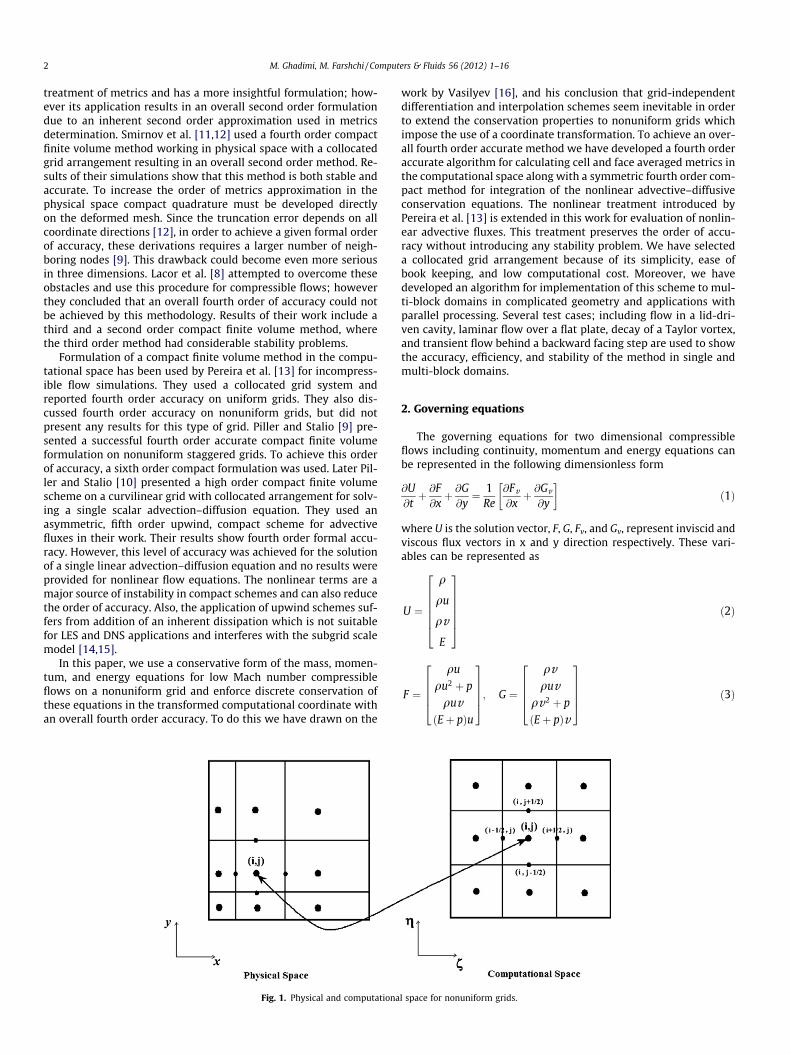
In this paper, we use a conservative form of the mass, momen-tum, and energy equations for low Mach number compressibleflows on a nonuniform grid and enforce discrete conservation ofthese equations in the transformed computational coordinate withan overall fourth order accuracy. To do this we have drawn on the

Fig. 1. Physical and computationa

work by Vasilyev [16], and his conclusion that grid-independentdifferentiation and interpolation schemes seem inevitable in orderto extend the conservation properties to nonuniform grids whichimpose the use of a coordinate transformation. To achieve an over-all fourth order accurate method we have developed a fourth orderaccurate algorithm for calculating cell and face averaged metrics inthe computational space along with a symmetric fourth order com-pact method for integration of the nonlinear advective–diffusiveconservation equations. The nonlinear treatment introduced byPereira et al. [13] is extended in this work for evaluation of nonlin-ear advective fluxes. This treatment preserves the order of accu-racy without introducing any stability problem. We have selecteda collocated grid arrangement because of its simplicity, ease ofbook keeping, and low computational cost. Moreover, we havedeveloped an algorithm for implementation of this scheme to mul-ti-block domains in complicated geometry and applications withparallel processing. Several test cases; including flow in a lid-dri-ven cavity, laminar flow over a flat plate, decay of a Taylor vortex,and transient flow behind a backward facing step are used to showthe accuracy, efficiency, and stability of the method in single andmulti-block domains.

2. Governing equations

The governing equations for two dimensional compressibleflows including continuity, momentum and energy equations canbe represented in the following dimensionless form

@U@tþ @F@xþ @G@y¼ 1

Re@Fv

@xþ @Gv

@y

� �ð1Þ

where U is the solution vector, F, G, Fv, and Gv, represent inviscid andviscous flux vectors in x and y direction respectively. These vari-ables can be represented as

U ¼

q

qu

qv

E

2666664

3777775 ð2Þ

F ¼

qu

qu2 þ p

quvðEþ pÞu

26664

37775; G ¼

qvquv

qv2 þ p

ðEþ pÞv

26664

37775 ð3Þ

l space for nonuniform grids.

M. Ghadimi, M. Farshchi / Computers & Fluids 56 (2012) 1–16 3

Fv ¼

0sxx

sxy

usxx þ vsxy � 1Prðc�1ÞM2

0qx

266664

377775; Gv ¼

0sxy

syy

usxy þ vsyy � 1Prðc�1ÞM2

0qy

266664

377775ð4Þ

with P ¼ ðc� 1Þ½E� 12 qðu2 þ v2Þ�

Here q is density, u and v are velocity components, p is pres-sure, and E is total energy per unit volume. Ideal gas relationsare used to relate pressure to density and total energy. Shear stresstensor components are represented by sxx, sxy, and syy. Heat fluxvector components are represented by qx and qy in x and y direc-tion respectively. Stokes stress law and Fourier heat transfer laware used for shear stress tensor and heat transfer vector determina-tion, respectively. The parameters Re, Pr, M0, and c represent Rey-nolds number, Prandtl number, Mach number, and specific heatratio respectively.

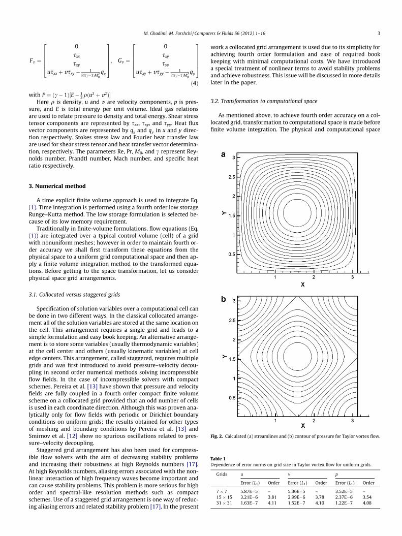
Fig. 2. Calculated (a) streamlines and (b) contour of pressure for Taylor vortex flow.

Table 1Dependence of error norms on grid size in Taylor vortex flow for uniform grids.

Grids u v p

Error (L1) Order Error (L1) Order Error (L1) Order

7 � 7 5.87E�5 – 5.36E�5 – 3.52E�5 –15 � 15 3.21E�6 3.81 2.99E�6 3.78 2.37E�6 3.5431 � 31 1.63E�7 4.11 1.52E�7 4.10 1.22E�7 4.08

3. Numerical method

A time explicit finite volume approach is used to integrate Eq.(1). Time integration is performed using a fourth order low storageRunge–Kutta method. The low storage formulation is selected be-cause of its low memory requirement.

Traditionally in finite-volume formulations, flow equations (Eq.(1)) are integrated over a typical control volume (cell) of a gridwith nonuniform meshes; however in order to maintain fourth or-der accuracy we shall first transform these equations from thephysical space to a uniform grid computational space and then ap-ply a finite volume integration method to the transformed equa-tions. Before getting to the space transformation, let us considerphysical space grid arrangements.

3.1. Collocated versus staggered grids

Specification of solution variables over a computational cell canbe done in two different ways. In the classical collocated arrange-ment all of the solution variables are stored at the same location onthe cell. This arrangement requires a single grid and leads to asimple formulation and easy book keeping. An alternative arrange-ment is to store some variables (usually thermodynamic variables)at the cell center and others (usually kinematic variables) at celledge centers. This arrangement, called staggered, requires multiplegrids and was first introduced to avoid pressure–velocity decou-pling in second order numerical methods solving incompressibleflow fields. In the case of incompressible solvers with compactschemes, Pereira et al. [13] have shown that pressure and velocityfields are fully coupled in a fourth order compact finite volumescheme on a collocated grid provided that an odd number of cellsis used in each coordinate direction. Although this was proven ana-lytically only for flow fields with periodic or Dirichlet boundaryconditions on uniform grids; the results obtained for other typesof meshing and boundary conditions by Pereira et al. [13] andSmirnov et al. [12] show no spurious oscillations related to pres-sure–velocity decoupling.

Staggered grid arrangement has also been used for compress-ible flow solvers with the aim of decreasing stability problemsand increasing their robustness at high Reynolds numbers [17].At high Reynolds numbers, aliasing errors associated with the non-linear interaction of high frequency waves become important andcan cause stability problems. This problem is more serious for highorder and spectral-like resolution methods such as compactschemes. Use of a staggered grid arrangement is one way of reduc-ing aliasing errors and related stability problem [17]. In the present

work a collocated grid arrangement is used due to its simplicity forachieving fourth order formulation and ease of required bookkeeping with minimal computational costs. We have introduceda special treatment of nonlinear terms to avoid stability problemsand achieve robustness. This issue will be discussed in more detailslater in the paper.

3.2. Transformation to computational space

As mentioned above, to achieve fourth order accuracy on a col-located grid, transformation to computational space is made beforefinite volume integration. The physical and computational space

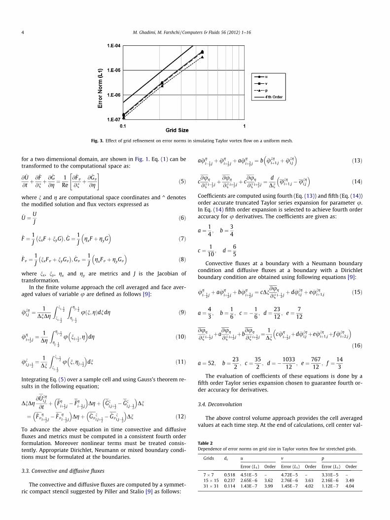
Fig. 3. Effect of grid refinement on error norms in simulating Taylor vortex flow on a uniform mesh.

Table 2Dependence of error norms on grid size in Taylor vortex flow for stretched grids.

Grids dc u v p


7 � 7 0.518 4.51E�5 – 4.72E�5 – 3.31E�5 –15 � 15 0.237 2.65E�6 3.62 2.76E�6 3.63 2.16E�6 3.4931 � 31 0.114 1.43E�7 3.99 1.45E�7 4.02 1.12E�7 4.04


for a two dimensional domain, are shown in Fig. 1. Eq. (1) can betransformed to the computational space as:

@U@tþ @F@nþ @G@g¼ 1

Re@Fv

@nþ @Gv

@g

" #ð5Þ

where n and g are computational space coordinates and ^ denotesthe modified solution and flux vectors expressed as

U ¼ UJ

ð6Þ

F ¼ 1J

nxF þ nyG� �

; G ¼ 1J

gxF þ gyG� �

ð7Þ

Fv ¼1J

nxFv þ nyGv� �

; Gv ¼1J

gxFv þ gyGv

� �ð8Þ

where nx, ny, gx and gy are metrics and J is the Jacobian oftransformation.

In the finite volume approach the cell averaged and face aver-aged values of variable u are defined as follows [9]:

�ungi;j ¼

1DnDg

Z niþ1

2

ni�1

2

Z gjþ1

2

gj�1

2

uðn;gÞdndg ð9Þ

�ugiþ1

2;j¼ 1

Dg

Z gjþ1

2

gj�1

2

u niþ12;g

� �dg ð10Þ

�uni;jþ1

2¼ 1

Dn

Z niþ1

2

ni�1

2

u n;gjþ12

� �dn ð11Þ

Integrating Eq. (5) over a sample cell and using Gauss’s theorem re-sults in the following equation;

DnDg@Ung

i;j

@tþ Fg

iþ12;j� Fg

i�12;j

� �Dgþ Gn

i;jþ12� Gn

i;j�12

� �Dn

¼ Fvgiþ1

2;j� Fv

gi�1

2;j

� �Dgþ Gv

ni;jþ1

2� Gv

ni;j�1

2

� �Dn ð12Þ

To advance the above equation in time convective and diffusivefluxes and metrics must be computed in a consistent fourth orderformulation. Moreover nonlinear terms must be treated consis-tently. Appropriate Dirichlet, Neumann or mixed boundary condi-tions must be formulated at the boundaries.

3.3. Convective and diffusive fluxes

The convective and diffusive fluxes are computed by a symmet-ric compact stencil suggested by Piller and Stalio [9] as follows:

a �ugi�1

2;jþ �ug

iþ12;jþ a �ug

iþ32;j¼ b �ung

iþ1;j þ �ungi;j

� �ð13Þ

c@u@n

gi�1

2;jþ @u@n

giþ1

2;jþ c

@u@n

giþ3

2;j¼ d

Dnung

iþ1;j �ungi;j

� �ð14Þ

Coefficients are computed using fourth (Eq. (13)) and fifth (Eq. (14))order accurate truncated Taylor series expansion for parameter u.In Eq. (14) fifth order expansion is selected to achieve fourth orderaccuracy for u derivatives. The coefficients are given as:

a ¼ 14; b ¼ 3

4

c ¼ 110

; d ¼ 65

Convective fluxes at a boundary with a Neumann boundarycondition and diffusive fluxes at a boundary with a Dirichletboundary condition are obtained using following equations [9]:

�ugi�1

2;jþ a �ug

iþ12;jþ b �ug

iþ32;j¼ cDn

@u@n

gi�1

2;jþ d �ung

i;j þ e �ungiþ1;j ð15Þ

a ¼ 43; b ¼ 1

6; c ¼ �1

6; d ¼ 23

12; e ¼ 7

12

@u@n

gi�1

2;jþa

@u@n

giþ1

2;jþb

@u@n

giþ3

2;j¼ 1

Dnc �ug

i�12;jþd �ung

i;j þe �ungiþ1;jþ f �ung

iþ2;j

� �ð16Þ

a ¼ 52; b ¼ 232; c ¼ 35

2; d ¼ �1033

12; e ¼ 767

12; f ¼ 14

3

The evaluation of coefficients of these equations is done by afifth order Taylor series expansion chosen to guarantee fourth or-der accuracy for derivatives.

3.4. Deconvolution

The above control volume approach provides the cell averagedvalues at each time step. At the end of calculations, cell center val-

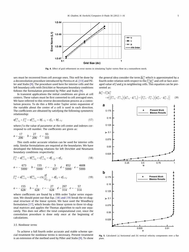
Fig. 5. Calculated (a) horizontal and (b) vertical velocity components over a flatplate.

Fig. 4. Effect of grid refinement on error norms in simulating Taylor vortex flow on a nonuniform mesh.


ues must be recovered from cell average ones. This will be done bya deconvolution procedure introduced by Pereira et al. [13] and Pil-ler and Stalio [9]. The procedure used here for interior cells and theleft boundary cells with Dirichlet or Neumann boundary conditionsfollows the formulation presented by Piller and Stalio [9].

In transient applications the initial conditions are given at cellcenters. These values must be first converted to cell averaged ones.We have referred to this reverse deconvolution process as a convo-lution process. To do this a fifth order Taylor series expansion ofthe variable about the center of a cell is used in each direction.The coefficients are obtained by satisfying the following symmetricrelationship:

a�f ngi�1;j þ �f ng

i;j þ a�f ngiþ1;j ¼ bfi�1;j þ cfi;j þ bfiþ1;j ð17Þ

where f is the value of parameter at the cell center and indexes cor-respond to cell number. The coefficients are given as:

a ¼ 17206

; b ¼ 27206

; c ¼ 93103

This sixth order accurate relation can be used for interior cellsonly. Similar formulations are required at the boundaries. We havedeveloped the following relations for left Dirichlet and Neumannboundary conditions respectively:

�f ngi;j þ a�f ng

iþ1;j þ b�f ngiþ2;j þ c�f ng

iþ3;j ¼ dfi�12;jþ efi;j ð18Þ

a ¼ � 6735999

; b ¼ 1555999

; c ¼ � 3857

; d ¼ 8525999

; e ¼ 46085999

�f ngi;j þ a�f ng

iþ1;j þ b�f ngiþ2;j ¼ cDn

@f@ni�1

2;jþ dfi;j þ efiþ1;j ð19Þ

a ¼ �155628

; b ¼ 7628

; c ¼ � 27628

; d ¼ 297314

; e ¼ � 57314

where coefficients are found by a fifth order Taylor series expan-sion. We should point out that Eqs. (18) and (19) break the tri-diag-onal structure of the linear system. We have used the Woodburyformulation [17], which breaks this linear system to three tri-diag-onal matrices and applies the Thomas algorithm to each one sepa-rately. This does not affect the total computational cost, since theconvolution procedure is done only once at the beginning ofcalculations.

3.5. Nonlinear terms

To achieve a full fourth order accurate and stable scheme spe-cial treatment for nonlinear terms is necessary. Present treatmentis an extension of the method used by Piller and Stalio [9]. To show

the general idea consider the term fgngi;j which is approximated by a

fourth order relation with respect to the f ngi;j gng

i;j and cell or face aver-aged value of f and g in neighboring cells. This equation can be pre-sented as:

�fgngi;j ¼�f ng

i;j�gng

i;j

þa �f ngiþ1;j��f ng

i�1;j

� ��gng

iþ1;j��gn;gi�1;j

� �þ �f n;g

i;jþ1��f ngi;j�1

� ��gng

i;jþ1��gngi;j�1

� �h ið20Þ


where the coefficient is obtained by applying a fourth order Taylorseries expansion of parameters f and g. In this case it results ina ¼ 1

48. To maintain fourth order accuracy at the boundaries withDirichlet and Neumann boundary conditions we have developedthe following equations respectively:

fgngi;j ¼�f ng

i;j�gng

i;j

þ 112

�f giþ1

2;j��f g

i�12;j

� ��gg

iþ12;j��gg

i�12;j

� �þ �f n

i;jþ12��f n

i;j�12

� ��gn

i;jþ12��gn

i;j�12

� �h ið21Þ

fgngi;j ¼�f ng

i;j�gng

i;j þ1

48@f@n

giþ1

2;jþ@f@n

gi�1

2;j

!@g@n

giþ1

2;jþ@g@n

gi�1

2;j

� Dn2

"

þ @f@g

ni;jþ1

2þ @f@g

ni;j�1

2

!@g@g

ni;jþ1

2þ@g@g

ni;j�1

2

� Dg2

#ð22Þ

We have also treated face averaged nonlinear terms which ap-pear in Eq. (12) in a similar manner resulting in formulations givenbelow:

fggiþ1

2;j¼ �f g

iþ12;j

�ggiþ1

2;jþ 1

48�f ng

i;jþ1 � �f ngi;j�1

� ��gng

i;jþ1 � �gngi;j�1

� �h ið23Þ

f@g@n

giþ1

2;j¼�f g

iþ12;j

@g@n

giþ1

2;j

þ 196Dn

�f ngi;jþ1��f ng

i;j�1

� ��gng

iþ1;jþ1��gngiþ1;j�1��gng

i�1;jþ1þ�gngi�1;j�1

� �h ið24Þ

f@g@g

giþ1

2;j¼ �f g

iþ12;j

@g@g

giþ1

2;j

þ 124Dg

�f ngi;jþ1 � �f ng

i;j�1

� ��gng

i;jþ1 � 2�gngi;j þ bargng

i;j�1

� �h ið25Þ

Appendix A contains additional formulations for triple productsand products in three-dimensional space. This treatment reduces

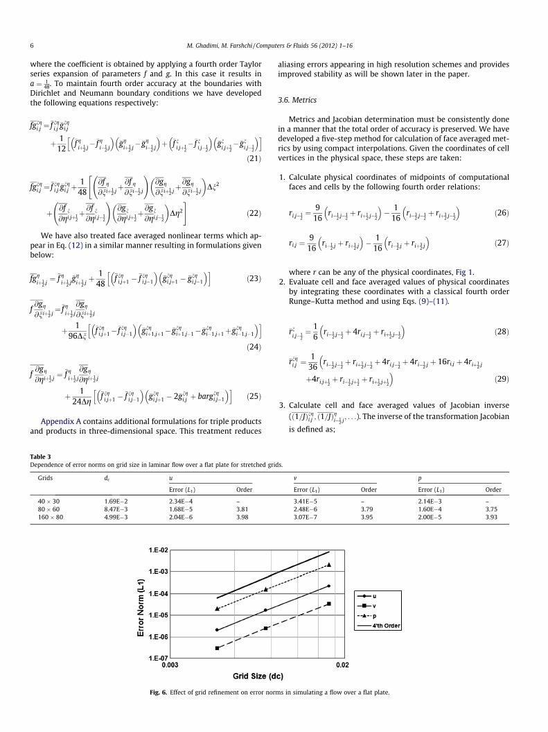
Fig. 6. Effect of grid refinement on error norm

Table 3Dependence of error norms on grid size in laminar flow over a flat plate for stretched grid

Grids dc u

Error (L1) Order

40 � 30 1.69E�2 2.34E�4 –80 � 60 8.47E�3 1.68E�5 3.81160 � 80 4.99E�3 2.04E�6 3.98

aliasing errors appearing in high resolution schemes and providesimproved stability as will be shown later in the paper.

3.6. Metrics

Metrics and Jacobian determination must be consistently donein a manner that the total order of accuracy is preserved. We havedeveloped a five-step method for calculation of face averaged met-rics by using compact interpolations. Given the coordinates of cellvertices in the physical space, these steps are taken:

1. Calculate physical coordinates of midpoints of computationalfaces and cells by the following fourth order relations:

ri;j�12¼ 9

16ri�1

2;j�12þ riþ1

2;j�12

� �� 1

16ri�3

2;j�12þ riþ3

2;j�12

� �ð26Þ

ri;j ¼9

16ri�1

2;jþ riþ1

2;j

� �� 1

16ri�3

2;jþ riþ3

2;j

� �ð27Þ

where r can be any of the physical coordinates, Fig 1.2. Evaluate cell and face averaged values of physical coordinates

by integrating these coordinates with a classical fourth orderRunge–Kutta method and using Eqs. (9)–(11).

�rni;j�1

2¼ 1

6ri�1

2;j�12þ 4ri;j�1

2þ riþ1

2;j�12

� �ð28Þ

�rngi;j ¼

136

ri�12;j�

12þ riþ1

2;j�12þ 4ri;j�1

2þ 4ri�1

2;jþ 16ri;j þ 4riþ1

2;j

�þ4ri;jþ1

2þ ri�1

2;jþ12þ riþ1

2;jþ12

�ð29Þ

3. Calculate cell and face averaged values of Jacobian inverse(ð1=JÞngi;j ; ð1=JÞg

i�12;j; . . .). The inverse of the transformation Jacobian

is defined as;

s in simulating a flow over a flat plate.

s.

v p

Error (L1) Order Error (L1) Order

3.41E�5 – 2.14E�3 –2.48E�6 3.79 1.60E�4 3.753.07E�7 3.95 2.00E�5 3.93

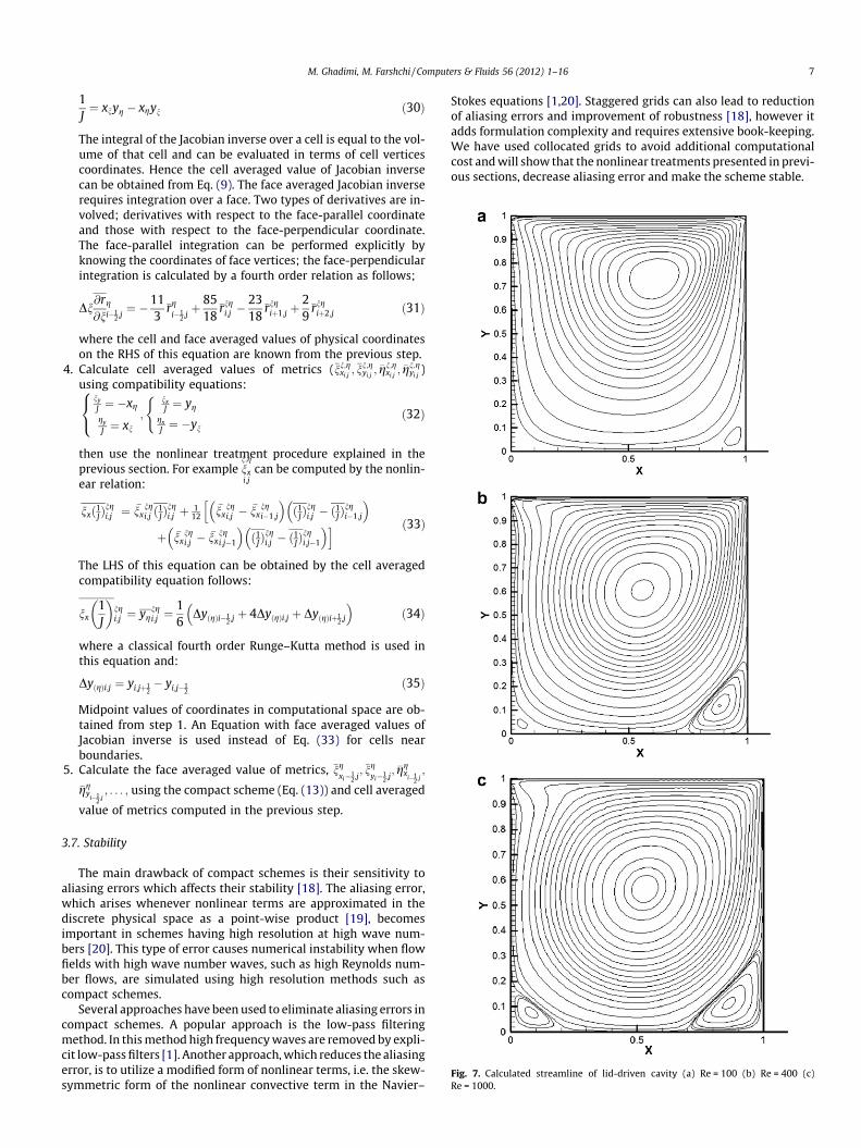
Fig. 7. Calculated streamline of lid-driven cavity (a) Re = 100 (b) Re = 400 (c)Re = 1000.


1J¼ xnyg � xgyn ð30Þ

The integral of the Jacobian inverse over a cell is equal to the vol-ume of that cell and can be evaluated in terms of cell verticescoordinates. Hence the cell averaged value of Jacobian inversecan be obtained from Eq. (9). The face averaged Jacobian inverserequires integration over a face. Two types of derivatives are in-volved; derivatives with respect to the face-parallel coordinateand those with respect to the face-perpendicular coordinate.The face-parallel integration can be performed explicitly byknowing the coordinates of face vertices; the face-perpendicularintegration is calculated by a fourth order relation as follows;

Dn@r@n

gi�1

2;j¼ �11

3�rg

i�12;jþ 85

18�rng

i;j �2318

�rngiþ1;j þ

29

�rngiþ2;j ð31Þ

where the cell and face averaged values of physical coordinateson the RHS of this equation are known from the previous step.

4. Calculate cell averaged values of metrics (�nn;gxi;j; �nn;g

yi;j; �gn;g

xi;j; �gn;g

yi;j)

using compatibility equations:ny

J ¼ �xg

gy

J ¼ xn

8<: ;

nxJ ¼ yg

gxJ ¼ �yn

(ð32Þ

then use the nonlinear treatment procedure explained in theprevious section. For example nx

n;g

i;jcan be computed by the nonlin-

ear relation:

nxð1JÞngi;j ¼ �nx

ngi;j ð1JÞ

ngi;j þ 1

12�nx

ngi;j � �nx

ngi�1;j

� �ð1JÞ

ngi;j � ð1JÞ

ngi�1;j

� �hþ �nx

ngi;j � �nx

ngi;j�1

� �ð1JÞ

ngi;j � ð1JÞ

ngi;j�1

� �i ð33Þ

The LHS of this equation can be obtained by the cell averagedcompatibility equation follows:

nx1J

� ngi;j ¼ yg

ngi;j ¼

16

DyðgÞi�12;jþ 4DyðgÞi;j þ DyðgÞiþ1

2;j

� �ð34Þ

where a classical fourth order Runge–Kutta method is used inthis equation and:

DyðgÞi;j ¼ yi;jþ12� yi;j�1

2ð35Þ

Midpoint values of coordinates in computational space are ob-tained from step 1. An Equation with face averaged values ofJacobian inverse is used instead of Eq. (33) for cells nearboundaries.

5. Calculate the face averaged value of metrics, �ngxi�1

2;j; �ng

yi�12;j; �gg

xi�1

2;j;

�ggy

i�12;j; . . . ; using the compact scheme (Eq. (13)) and cell averaged

value of metrics computed in the previous step.

3.7. Stability

The main drawback of compact schemes is their sensitivity toaliasing errors which affects their stability [18]. The aliasing error,which arises whenever nonlinear terms are approximated in thediscrete physical space as a point-wise product [19], becomesimportant in schemes having high resolution at high wave num-bers [20]. This type of error causes numerical instability when flowfields with high wave number waves, such as high Reynolds num-ber flows, are simulated using high resolution methods such ascompact schemes.

Several approaches have been used to eliminate aliasing errors incompact schemes. A popular approach is the low-pass filteringmethod. In this method high frequency waves are removed by expli-cit low-pass filters [1]. Another approach, which reduces the aliasingerror, is to utilize a modified form of nonlinear terms, i.e. the skew-symmetric form of the nonlinear convective term in the Navier–

Stokes equations [1,20]. Staggered grids can also lead to reductionof aliasing errors and improvement of robustness [18], however itadds formulation complexity and requires extensive book-keeping.We have used collocated grids to avoid additional computationalcost and will show that the nonlinear treatments presented in previ-ous sections, decrease aliasing error and make the scheme stable.

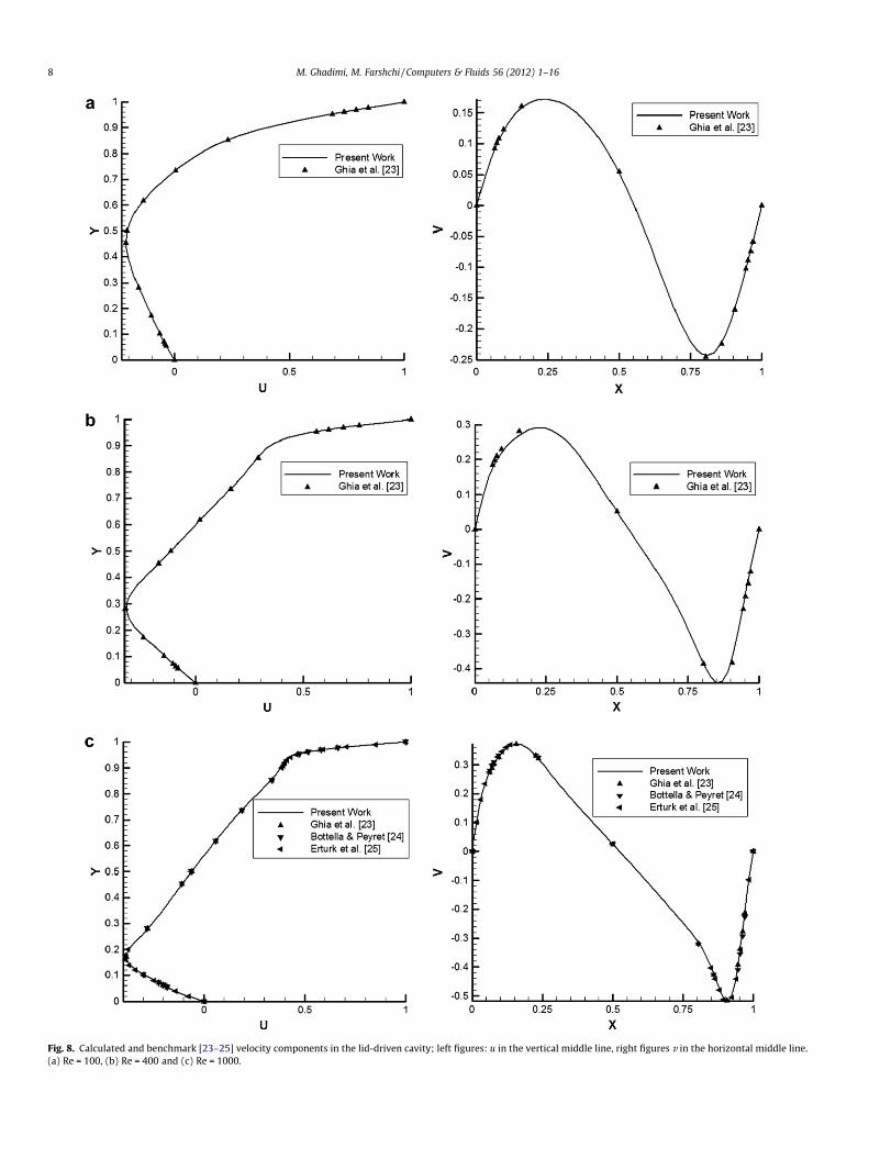
Fig. 8. Calculated and benchmark [23–25] velocity components in the lid-driven cavity; left figures: u in the vertical middle line, right figures v in the horizontal middle line.(a) Re = 100, (b) Re = 400 and (c) Re = 1000.


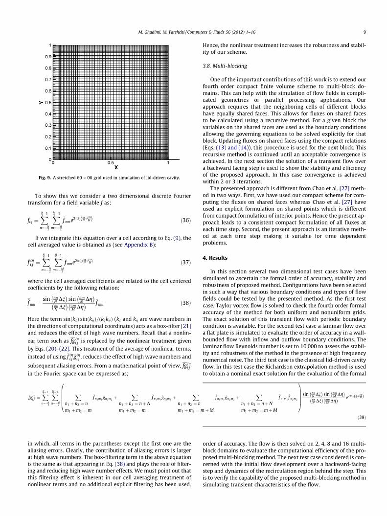
Fig. 9. A stretched 60 � 06 grid used in simulation of lid-driven cavity.


To show this we consider a two dimensional discrete Fouriertransform for a field variable f as:

fi;j ¼XN2�1

n¼�N2

XM2�1

m¼�M2

f nme2pic inNþ

jmMð Þ ð36Þ

If we integrate this equation over a cell according to Eq. (9), thecell averaged value is obtained as (see Appendix B):

�f ngi;j ¼

XN2�1

n¼�N2

XM2�1

m¼�M2

f nme2pic ðinNþjmMÞ ð37Þ

where the cell averaged coefficients are related to the cell centeredcoefficients by the following relation:

f nm ¼sin pn

N Dn� �

sin pmM Dg� �

pnN Dn� �

pmM Dg� � f mn ð38Þ

Here the term sinðknÞ sinðkgÞ=ðknkgÞ (kn and kg are wave numbers inthe directions of computational coordinates) acts as a box-filter [21]and reduces the effect of high wave numbers. Recall that a nonlin-

ear term such as fgngi;j is replaced by the nonlinear treatment given

by Eqs. (20)–(22). This treatment of the average of nonlinear terms,

instead of using f ngi;j gng

i;j , reduces the effect of high wave numbers and

subsequent aliasing errors. From a mathematical point of view, fgngi;j

in the Fourier space can be expressed as;

fgngi;j ¼

XN2�1

n¼�N2

XM2�1

m¼�M2

Xn1 þ n2 ¼ n

m1 þm2 ¼ m

f n1m1 gn2 m2 þX

n1 þ n2 ¼ nþ N

m1 þm2 ¼ m

f n1 m1 gn2 m2 þX

n1 þ n2 ¼ n

m1 þm2 ¼ mþM

f n1 m1 gn2 m2 þX

n1 þ n2 ¼ nþ N

m1 þm2 ¼ mþM

f n1 m1 f n2 m2

0BBBBB@

1CCCCCA

sin pnN Dn� �

sin pmM Dg� �

pnN Dn� �

pmM Dg� � e2pic in

NþjmMð Þ

ð39Þ

in which, all terms in the parentheses except the first one are thealiasing errors. Clearly, the contribution of aliasing errors is largerat high wave numbers. The box-filtering term in the above equationis the same as that appearing in Eq. (38) and plays the role of filter-ing and reducing high wave number effects. We must point out thatthis filtering effect is inherent in our cell averaging treatment ofnonlinear terms and no additional explicit filtering has been used.

Hence, the nonlinear treatment increases the robustness and stabil-ity of our scheme.

3.8. Multi-blocking

One of the important contributions of this work is to extend ourfourth order compact finite volume scheme to multi-block do-mains. This can help with the simulation of flow fields in compli-cated geometries or parallel processing applications. Ourapproach requires that the neighboring cells of different blockshave equally shared faces. This allows for fluxes on shared facesto be calculated using a recursive method. For a given block thevariables on the shared faces are used as the boundary conditionsallowing the governing equations to be solved explicitly for thatblock. Updating fluxes on shared faces using the compact relations(Eqs. (13) and (14)), this procedure is used for the next block. Thisrecursive method is continued until an acceptable convergence isachieved. In the next section the solution of a transient flow overa backward facing step is used to show the stability and efficiencyof the proposed approach. In this case convergence is achievedwithin 2 or 3 iterations.

The presented approach is different from Chao et al. [27] meth-od in two ways. First, we have used our compact scheme for com-puting the fluxes on shared faces whereas Chao et al. [27] haveused an explicit formulation on shared points which is differentfrom compact formulation of interior points. Hence the present ap-proach leads to a consistent compact formulation of all fluxes ateach time step. Second, the present approach is an iterative meth-od at each time step making it suitable for time dependentproblems.

4. Results

In this section several two dimensional test cases have beensimulated to ascertain the formal order of accuracy, stability androbustness of proposed method. Configurations have been selectedin such a way that various boundary conditions and types of flowfields could be tested by the presented method. As the first testcase, Taylor vortex flow is solved to check the fourth order formalaccuracy of the method for both uniform and nonuniform grids.The exact solution of this transient flow with periodic boundarycondition is available. For the second test case a laminar flow overa flat plate is simulated to evaluate the order of accuracy in a wall-bounded flow with inflow and outflow boundary conditions. Thelaminar flow Reynolds number is set to 10,000 to assess the stabil-ity and robustness of the method in the presence of high frequencynumerical noise. The third test case is the classical lid-driven cavityflow. In this test case the Richardson extrapolation method is usedto obtain a nominal exact solution for the evaluation of the formal

order of accuracy. The flow is then solved on 2, 4, 8 and 16 multi-block domains to evaluate the computational efficiency of the pro-posed multi-blocking method. The next test case considered is con-cerned with the initial flow development over a backward-facingstep and dynamics of the recirculation region behind the step. Thisis to verify the capability of the proposed multi-blocking method insimulating transient characteristics of the flow.

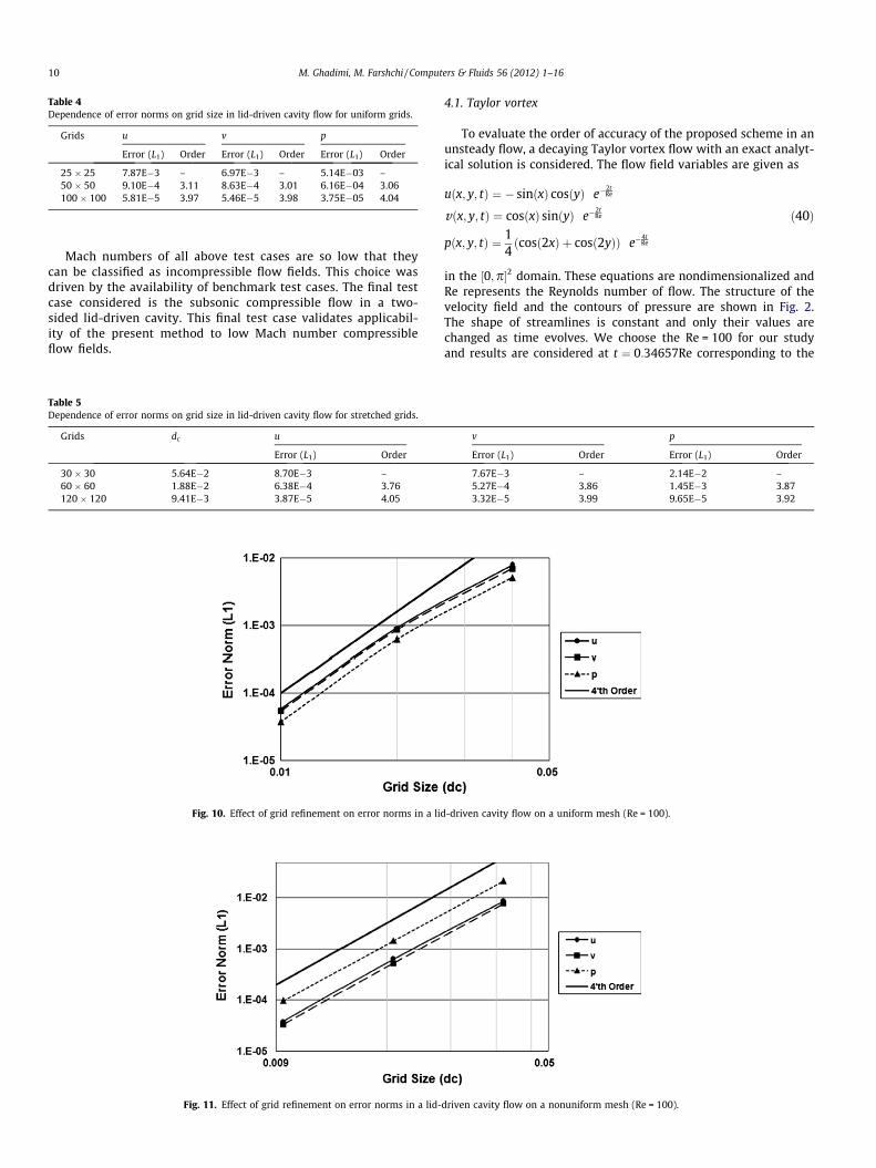
Table 4Dependence of error norms on grid size in lid-driven cavity flow for uniform grids.

Grids u v p


25 � 25 7.87E�3 – 6.97E�3 – 5.14E�03 –50 � 50 9.10E�4 3.11 8.63E�4 3.01 6.16E�04 3.06100 � 100 5.81E�5 3.97 5.46E�5 3.98 3.75E�05 4.04


Mach numbers of all above test cases are so low that theycan be classified as incompressible flow fields. This choice wasdriven by the availability of benchmark test cases. The final testcase considered is the subsonic compressible flow in a two-sided lid-driven cavity. This final test case validates applicabil-ity of the present method to low Mach number compressibleflow fields.

Fig. 11. Effect of grid refinement on error norms in a lid-

Fig. 10. Effect of grid refinement on error norms in a lid

Table 5Dependence of error norms on grid size in lid-driven cavity flow for stretched grids.

Grids dc u

Error (L1) Order

30 � 30 5.64E�2 8.70E�3 –60 � 60 1.88E�2 6.38E�4 3.76120 � 120 9.41E�3 3.87E�5 4.05

4.1. Taylor vortex

To evaluate the order of accuracy of the proposed scheme in anunsteady flow, a decaying Taylor vortex flow with an exact analyt-ical solution is considered. The flow field variables are given as

uðx; y; tÞ ¼ � sinðxÞ cosðyÞ e�2tRe

vðx; y; tÞ ¼ cosðxÞ sinðyÞ e�2tRe ð40Þ

pðx; y; tÞ ¼ 14ðcosð2xÞ þ cosð2yÞÞ e�

4tRe

in the ½0;p�2 domain. These equations are nondimensionalized andRe represents the Reynolds number of flow. The structure of thevelocity field and the contours of pressure are shown in Fig. 2.The shape of streamlines is constant and only their values arechanged as time evolves. We choose the Re = 100 for our studyand results are considered at t ¼ 0:34657Re corresponding to the

driven cavity flow on a nonuniform mesh (Re = 100).

-driven cavity flow on a uniform mesh (Re = 100).

v p

Error (L1) Order Error (L1) Order

7.67E�3 – 2.14E�2 –5.27E�4 3.86 1.45E�3 3.873.32E�5 3.99 9.65E�5 3.92

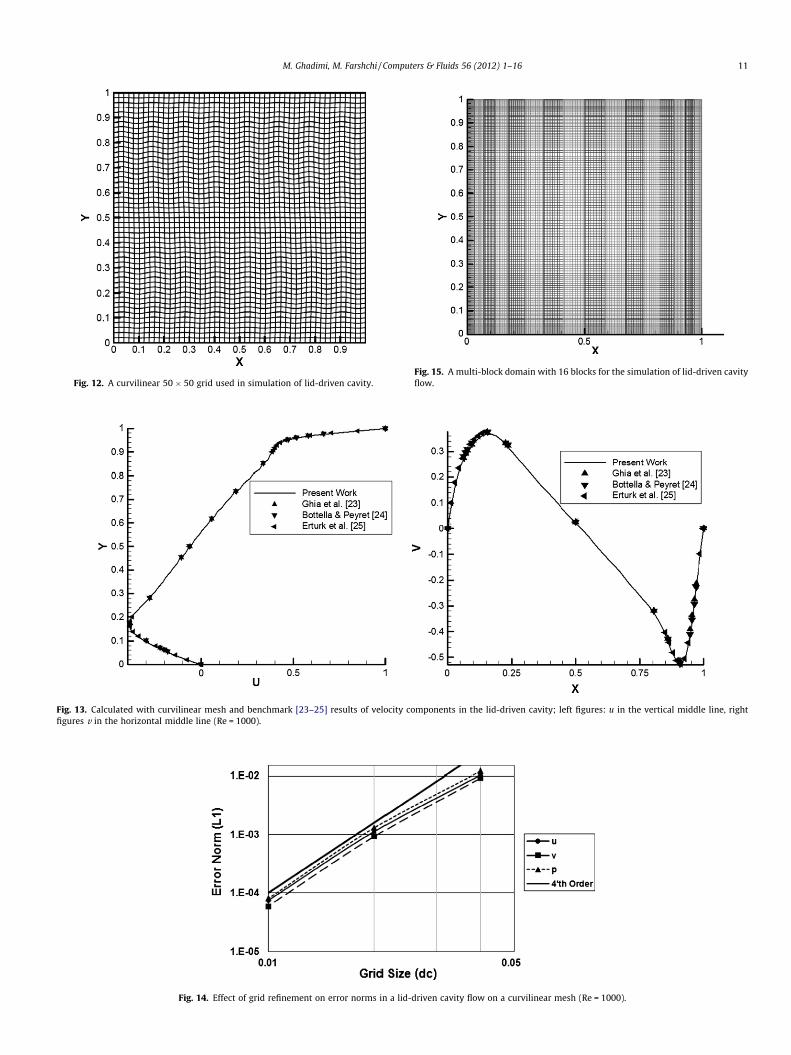
Fig. 14. Effect of grid refinement on error norms in a lid-driven cavity flow on a curvilinear mesh (Re = 1000).

Fig. 13. Calculated with curvilinear mesh and benchmark [23–25] results of velocity components in the lid-driven cavity; left figures: u in the vertical middle line, rightfigures v in the horizontal middle line (Re = 1000).

Fig. 12. A curvilinear 50 � 50 grid used in simulation of lid-driven cavity.Fig. 15. A multi-block domain with 16 blocks for the simulation of lid-driven cavityflow.


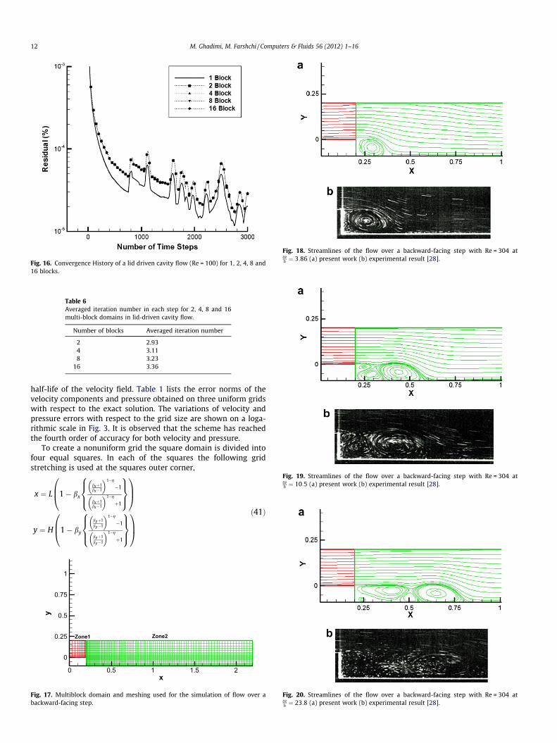
Fig. 16. Convergence History of a lid driven cavity flow (Re = 100) for 1, 2, 4, 8 and16 blocks.

Table 6Averaged iteration number in each step for 2, 4, 8 and 16multi-block domains in lid-driven cavity flow.

Number of blocks Averaged iteration number

2 2.934 3.118 3.23

16 3.36

Fig. 18. Streamlines of the flow over a backward-facing step with Re = 304 atUth ¼ 3:86 (a) present work (b) experimental result [28].



half-life of the velocity field. Table 1 lists the error norms of thevelocity components and pressure obtained on three uniform gridswith respect to the exact solution. The variations of velocity andpressure errors with respect to the grid size are shown on a loga-rithmic scale in Fig. 3. It is observed that the scheme has reachedthe fourth order of accuracy for both velocity and pressure.

To create a nonuniform grid the square domain is divided intofour equal squares. In each of the squares the following gridstretching is used at the squares outer corner,

x ¼ L 1� bx

bxþ1bx�1

� �1�g

�1

bxþ1bx�1

� �1�g

þ1

8><>:

9>=>;

0B@

1CA

y ¼ H 1� by

byþ1by�1

� �1�g

�1

byþ1by�1

� �1�g

þ1

8><>:

9>=>;

0B@

1CA

ð41Þ

x

y

0 0.5 1 1.5 2

0

0.25

0.5

0.75

1

Zone1 Zone2

Fig. 17. Multiblock domain and meshing used for the simulation of flow over abackward-facing step.


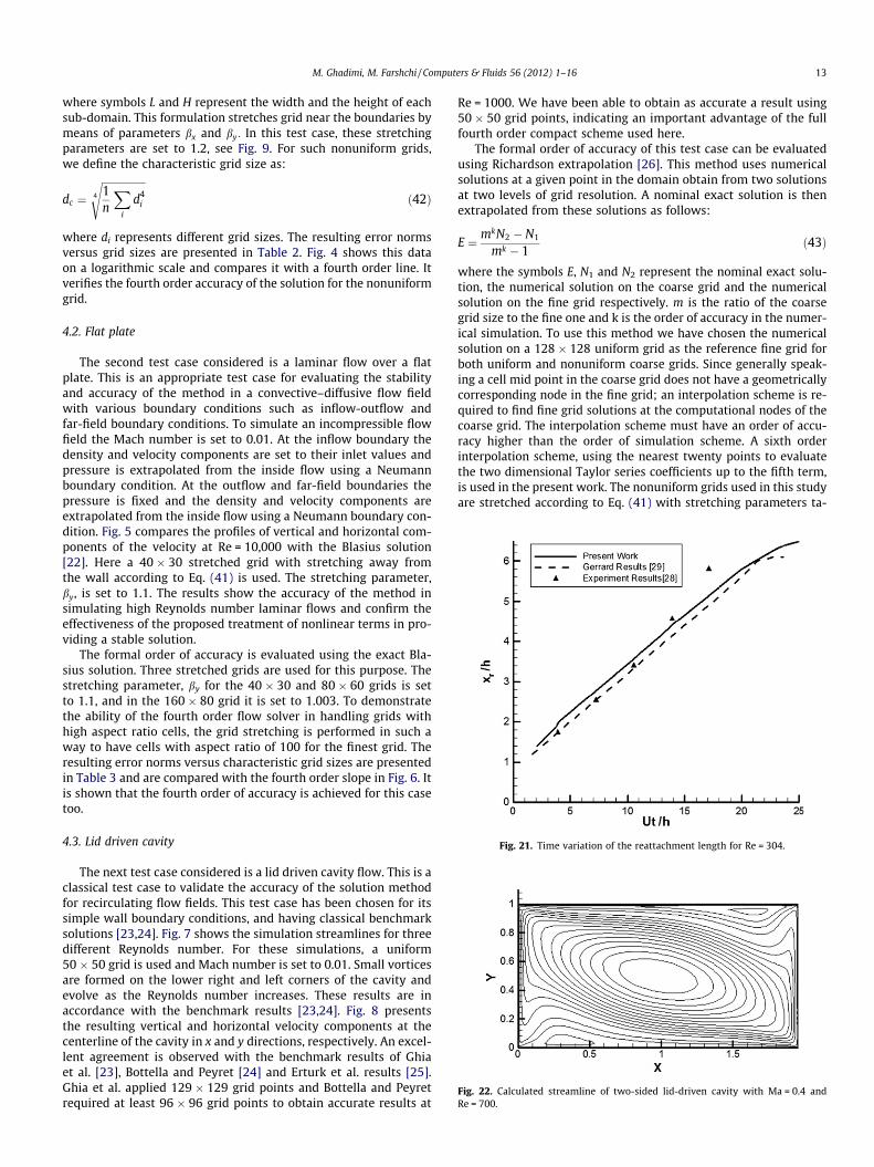
Fig. 22. Calculated streamline of two-sided lid-driven cavity with Ma = 0.4 andRe = 700.

Fig. 21. Time variation of the reattachment length for Re = 304.


where symbols L and H represent the width and the height of eachsub-domain. This formulation stretches grid near the boundaries bymeans of parameters bx and by: In this test case, these stretchingparameters are set to 1.2, see Fig. 9. For such nonuniform grids,we define the characteristic grid size as:

dc ¼ffiffiffiffiffiffiffiffiffiffiffiffiffiffiffiffiffi1n

Xi

d4i

4

sð42Þ

where di represents different grid sizes. The resulting error normsversus grid sizes are presented in Table 2. Fig. 4 shows this dataon a logarithmic scale and compares it with a fourth order line. Itverifies the fourth order accuracy of the solution for the nonuniformgrid.

4.2. Flat plate

The second test case considered is a laminar flow over a flatplate. This is an appropriate test case for evaluating the stabilityand accuracy of the method in a convective–diffusive flow fieldwith various boundary conditions such as inflow-outflow andfar-field boundary conditions. To simulate an incompressible flowfield the Mach number is set to 0.01. At the inflow boundary thedensity and velocity components are set to their inlet values andpressure is extrapolated from the inside flow using a Neumannboundary condition. At the outflow and far-field boundaries thepressure is fixed and the density and velocity components areextrapolated from the inside flow using a Neumann boundary con-dition. Fig. 5 compares the profiles of vertical and horizontal com-ponents of the velocity at Re = 10,000 with the Blasius solution[22]. Here a 40 � 30 stretched grid with stretching away fromthe wall according to Eq. (41) is used. The stretching parameter,by, is set to 1.1. The results show the accuracy of the method insimulating high Reynolds number laminar flows and confirm theeffectiveness of the proposed treatment of nonlinear terms in pro-viding a stable solution.

The formal order of accuracy is evaluated using the exact Bla-sius solution. Three stretched grids are used for this purpose. Thestretching parameter, by for the 40 � 30 and 80 � 60 grids is setto 1.1, and in the 160 � 80 grid it is set to 1.003. To demonstratethe ability of the fourth order flow solver in handling grids withhigh aspect ratio cells, the grid stretching is performed in such away to have cells with aspect ratio of 100 for the finest grid. Theresulting error norms versus characteristic grid sizes are presentedin Table 3 and are compared with the fourth order slope in Fig. 6. Itis shown that the fourth order of accuracy is achieved for this casetoo.

4.3. Lid driven cavity

The next test case considered is a lid driven cavity flow. This is aclassical test case to validate the accuracy of the solution methodfor recirculating flow fields. This test case has been chosen for itssimple wall boundary conditions, and having classical benchmarksolutions [23,24]. Fig. 7 shows the simulation streamlines for threedifferent Reynolds number. For these simulations, a uniform50 � 50 grid is used and Mach number is set to 0.01. Small vorticesare formed on the lower right and left corners of the cavity andevolve as the Reynolds number increases. These results are inaccordance with the benchmark results [23,24]. Fig. 8 presentsthe resulting vertical and horizontal velocity components at thecenterline of the cavity in x and y directions, respectively. An excel-lent agreement is observed with the benchmark results of Ghiaet al. [23], Bottella and Peyret [24] and Erturk et al. results [25].Ghia et al. applied 129 � 129 grid points and Bottella and Peyretrequired at least 96 � 96 grid points to obtain accurate results at

Re = 1000. We have been able to obtain as accurate a result using50 � 50 grid points, indicating an important advantage of the fullfourth order compact scheme used here.

The formal order of accuracy of this test case can be evaluatedusing Richardson extrapolation [26]. This method uses numericalsolutions at a given point in the domain obtain from two solutionsat two levels of grid resolution. A nominal exact solution is thenextrapolated from these solutions as follows:

E ¼ mkN2 � N1

mk � 1ð43Þ

where the symbols E, N1 and N2 represent the nominal exact solu-tion, the numerical solution on the coarse grid and the numericalsolution on the fine grid respectively. m is the ratio of the coarsegrid size to the fine one and k is the order of accuracy in the numer-ical simulation. To use this method we have chosen the numericalsolution on a 128 � 128 uniform grid as the reference fine grid forboth uniform and nonuniform coarse grids. Since generally speak-ing a cell mid point in the coarse grid does not have a geometricallycorresponding node in the fine grid; an interpolation scheme is re-quired to find fine grid solutions at the computational nodes of thecoarse grid. The interpolation scheme must have an order of accu-racy higher than the order of simulation scheme. A sixth orderinterpolation scheme, using the nearest twenty points to evaluatethe two dimensional Taylor series coefficients up to the fifth term,is used in the present work. The nonuniform grids used in this studyare stretched according to Eq. (41) with stretching parameters ta-


ken to be 1.2 in both directions. Fig. 9 shows a sample 60 � 60 non-uniform stretched grid used for the above case.

The grid sizes and error norms of velocity components and pres-sure for the Reynolds number of 100 on uniform and nonuniformgrids are shown in Tables 4 and 5 respectively. The formal orderof accuracy for each grid is computed and presented in these ta-bles. Results indicate that the fourth order of accuracy is reachedon both uniform and nonuniform grids. Figs. 10 and 11 show thevariation of these error norms with respect to the characteristicgrid sizes in the logarithmic scale for uniform and nonuniformgrids respectively.

We have also demonstrated the solver competence on a curvi-linear grid for this type of flow. Fig. 12 shows a fully curvilinear50 � 50 grid. This grid has been generated by the followingrelations:

xi;j ¼ �xi;j þ 0:02 ði�ieÞði�imidÞimid2 sinð2p�yi;jÞ

yi;j ¼ �yi;j þ 0:02 ðj�jeÞðj�jmidÞj2mid

sinð16p�xi;jÞð44Þ

In which �xi;j and �yi;j denote coordinates of the correspondinguniform grid. The numbers imid and ie are the half number of gridsin x direction and the edge number defined as follows:

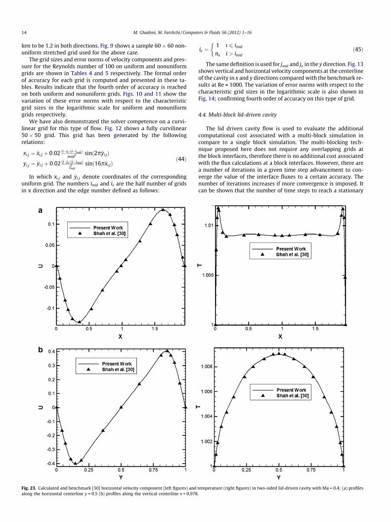
Fig. 23. Calculated and benchmark [30] horizontal velocity component (left figures) andalong the horizontal centerline y = 0.5 (b) profiles along the vertical centerline x = 0.978

ie ¼1 ı 6 imid

nx i > imid

�ð45Þ

The same definition is used for jmid and je in the y direction. Fig. 13shows vertical and horizontal velocity components at the centerlineof the cavity in x and y directions compared with the benchmark re-sults at Re = 1000. The variation of error norms with respect to thecharacteristic grid sizes in the logarithmic scale is also shown inFig. 14; confirming fourth order of accuracy on this type of grid.

4.4. Multi-block lid-driven cavity

The lid driven cavity flow is used to evaluate the additionalcomputational cost associated with a multi-block simulation incompare to a single block simulation. The multi-blocking tech-nique proposed here does not require any overlapping grids atthe block interfaces, therefore there is no additional cost associatedwith the flux calculations at a block interfaces. However, there area number of iterations in a given time step advancement to con-verge the value of the interface fluxes to a certain accuracy. Thenumber of iterations increases if more convergence is imposed. Itcan be shown that the number of time steps to reach a stationary

temperature (right figures) in two-sided lid-driven cavity with Ma = 0.4; (a) profiles.


solution can be increased to compensate for a low convergencerequirement of the interface fluxes. The blocks are arranged in a se-rial manner here. Fig. 15 shows a 128 � 128 stretched grid andblocks arrangement for solving the flow in a cavity with 16 blocks.Fig. 16 compares the convergence history of the lid-driven cavityflow for a single block domain versus 2, 4, 8, and 16 multi-blockdomains for the case of Re = 100. Here the local interface flux con-vergence is reached when the percentage of error in interfacefluxes reduces to about 5% of the local residual. Table 6 presentsthe average iteration numbers in each time step for the 2, 4, 8and 16 blocks. These iteration numbers are calculated for a128 � 128 grid. Adopting the Chao et al. [27] definition of compu-tational efficiency of a multi-block approach for parallel process-ing, based on results presented in Table 6, we obtain anestimated computational efficiency of 79% for the 16 blocks, whichis comparable to the their computational efficiency.

4.5. Laminar flow behind a backward-facing step

The next test case is the flow behind a backward-facing step withthe aim of testing applicability of the scheme in solving unsteadyflows in multi-block domains. In this type of flow, fluid flow is sep-arated from the wall due to suddenly expanded geometry and the re-sulted shear layer is reattached to the wall somewhere downstreamof the step and develops a recirculating zone. The characteristiclength of reattachment zone in the direction of flow and the numberof vortices in this zone for unsteady flow are functions of the Rey-nolds number and time of evolution [28]. The multi-block grid usedfor the simulation of this flow is shown in Fig. 17. As observed in thisfigure, a relatively coarse grid (a 10 � 10 grid before and a 100 � 20grid after step) is applied in this simulation. A symmetric boundarycondition has been used for the upper boundary in which the verticalcomponent of velocity is set to zero and the horizontal component ofvelocity, density and pressure are extrapolated from the inside flowusing a Neumann boundary condition. The Reynolds number is setequal to 304 for comparison with the experimental results. Conver-gence of multi-block approach is achieved in each time step by onlytwo or three iteration.

The flow streamlines at three different nondimensionalizedtime intervals are compared with experimental results of Honji[28] Figs. 18–20. Time is nondimensionalized using the meanvelocity of flow at the inlet, U, and the step height, h. These figuresshow an excellent accordance of vortices’ shape and evolution withthe experimental results. The time variation of the reattachmentlocation is compared with experimental data of Honji [28] andnumerical results of Gerrard [29] in Fig. 21. The reattachmentlength xr is measured as the distance of reattachment location tothe step. It can be seen that results of the present work have a goodaccordance with the numerical results of Gerrard [29]. However,there is a discrepancy between numerical and experimental resultsat later times which can be due to three-dimensionality, develop-ing in the experiments at later times.

4.6. Compressible flow in a two-sided lid-driven cavity

All of the test cases considered so far are very low Mach numberflow cases. To show the presented method’s ability of simulatingcompressible flow fields we have selected a compressible flow ina two-sided lid-driven cavity [30]. The flow is generated by movingtwo opposing walls of a rectangular cavity in opposite directions.Its Prandtl number is 0.72 and its Mach number is 0.4. This wasthe highest Mach number used in the benchmark test case [30].The ratio of the horizontal side of the cavity to its vertical side is1.955. An 80 � 40 grid which is stretched near the walls accordingto Eq. (41) has been used in this test case. Stretching parameters inboth directions are set to the 1.2. Fig. 22 shows streamlines for the

Reynolds number of 700 which is in accordance with the bench-mark result [30]. Fig. 23 presents variations of horizontal velocitycomponent and temperature along the horizontal and vertical cen-terline of the cavity. The present results have an excellent agree-ment with the benchmark results of Shah et al. [30].

5. Conclusion

We have presented a fully fourth order symmetric (central)compact finite volume method on nonuniform grids which canbe used with multi-block domains. To achieve this we performeda coordinate transformation from the physical space to the compu-tational space and used a new fourth order method for calculatingcell and face averaged metrics. A new nonlinear treatment wasused to preserve the accuracy and stability of the solution method.We have also extended our method to simulation of flows in multi-block domains making it appropriate for complicated geometriesand parallel processing. Computational results for several testcases including; a decaying Taylor vortex, a laminar flow on a flatplate, and a lid-driven cavity flow, illustrate the fourth order for-mal accuracy and stability of this method for solving problemswith different boundary condition. Moreover, the solution of lid-driven cavity flow on multi-block domains and flow behind a back-ward facing step show the efficiency of presented approach formulti-block domains. The applicability of the present method tolow Mach number compressible flows was demonstrated by con-sidering a two-sided lid-driven cavity flow.

Appendix A. Treatment of nonlinear terms

The forth order formulation of nonlinear terms described in Sec-tion 3.5, can be extended to triple products as follows:

fghgi�1

2;j¼ f g

i�12;j

ggi�1

2;jhg

i�12;jþ 1

48hg

i�12;j

f gi�1

2;jþ1� f g

i�12;j�1

� �gg

i�12;jþ1� gg

i�12;j�1

� �h�gg

i�12;j

f gi�1

2;jþ1� f g

i�12;j�1

� �hg

i�12;jþ1�hg

i�12;j�1

� �þf g

i�12;j

ggi�1

2;jþ1� gg

i�12;j�1

� �hg

i�12;jþ1�hg

i�12;j�1

� �iðA:1Þ

This formulation can be derived explicitly or alternatively bytwice using Eq. (23) for the term ðfgÞhg

i�12;j

and then for the termðfgÞg

i�12;j

.

Treatment of nonlinear terms in three-dimensions is similar totheir two-dimensional counterpart, for example, Eq. (20) can bepresented as follows in three-dimension.

fgngfi;j;k ¼ f ngf

i;j;kgngfi;j;k þ

148

f ngfiþ1;j;k � f ngf

i�1;j;k

� �gngf

iþ1;j;k � gngfi�1;j;k

� �hþ f ngf

i;jþ1;k � f ngfi;j�1;k

� �gngf

i;jþ1;k � gngfi;j�1;k

� �þ f ngf

i;j;kþ1 � f ngfi;j;k�1

� �gngf

i;j;kþ1 � gngfi;j;k�1

� �iðA:2Þ

Appendix B. DFT of a cell-averaged variable

The Discrete Fourier transform of function f is defined by Eq.(36) of the paper:

fi;j ¼XN2�1

n¼�N2

XM2�1

m¼�M2

f nme2pic inNþ

jmMð Þ ðB:1Þ

On the other hand the cell averaged values of f is defined by Eq.(9) of the paper:

f ngi;j ¼

1DnDg

Z niþ1

2

ni�1

2

Z gjþ1

2

gj�1

2

f ðn;gÞdndg ðB:2Þ


Note that the computational space grid is uniform and the gridsize is equal to unity. Hence at point (i, j) in the computationalspace grid (n,g)ij = (iDn, jDg), where Dn = 1 and Dg = 1, therefore(n,g)ij = (i, j).

Transporting the origin of computational coordinates to the cellcenter, this integral can be stated as follows.

f ngi;j ¼

1DnDg

Z Dn2

�Dn2

Z Dg2

�Dg2

f ðiþ n; jþ gÞdndg ðB:3Þ

Substituting Eq. (B.1) in this relation, one can obtain:

f ngi;j ¼

1DnDg

Z Dn2

�Dn2

Z Dg2

�Dg2

XN2�1

n¼�N2

XM2�1

m¼�M2

f nme2picðiþnÞn

N þðjþgÞmMð Þ

0@

1Adndg ðB:4Þ

In this equation integrations can commute with summationsand double integrations can be performed independently due toseparability of the integrand. So one can obtain:

f ngi;j ¼

1DnDg

XN2�1

n¼�N2

XM2�1

m¼�M2

f nm

Z Dn2

�Dn2

Z Dg2

�Dg2

e2picðiþnÞn

N þðjþgÞmMð Þdndg

!

¼ 1DnDg

XN2�1

n¼�N2

XM2�1

m¼�M2

f nm

Z Dn2

�Dn2

e2picððiþnÞnN Þdn

! Z Dg2

�Dg2

e2picððjþgÞmM Þdg

!

¼XN2�1

n¼�N2

XM2�1

m¼�M2

f nme2pic inNþ

jmMð Þ 1

Dn

Z Dn2

�Dn2

e2picðnnN Þdn

!1

Dg

Z Dg2

�Dg2

e2pic ðgmM Þdg

!

ðB:5Þ

The integral terms can be computed as follows:

1Dn

R Dn2

�Dn2

e2picnnNð Þdn¼ 1

2pic nNð ÞDn

epicDnn

Nð Þ �e�picDnn

Nð Þ� �

¼ 1pnNð ÞDn

sin pnN Dn� �

&

1Dg

R Dg2

�Dg2

e2picgmMð Þdg¼ 1

2pic mMð ÞDg

epicDgm

Mð Þ �e�picDgm

Mð Þ� �

¼ 1pmMð ÞDg

sin pmM Dg� �ðB:6Þ

Substituting these relations in the Eq. (B.5), one can obtain:

f ngi;j ¼

XN2�1

n¼�N2

XM2�1

m¼�M2

f nmsin pn

N Dn� �

pnN Dn� � sinðpm

M DgÞpmM Dg� � e2pic in

NþjmMð Þ ðB:7Þ

References

[1] Meinke M, Schroder W, Krause E, Rister TH. A comparison of second- and sixth-order methods for large-eddy simulations. Comput Fluids 2002;31:695.

[2] Ghosal S. An analysis of numerical errors in large eddy simulation ofturbulence. J Comp Phys 1996;125:187.

[3] Hoffmann KA, Chiang ST. Computational fluid dynamics for engineers. Wichita(KS): Engineering Education System; 1993.

[4] Mattiussi B. An analysis of finite volume, finite element, and finite differencemethods using some concepts from algebraic topology. J Comp Phys1997;133(2):289.

[5] Hirsch C. Numerical computation of internal and external flows. WestSussex: Wiley; 1994.

[6] Gaitonde D, Shang JS. Optimized compact-difference-based finite-volumeschemes for linear wave phenomena. J Comp Phys 1997;138:617.

[7] Kobayashi MH. On a class of Pade finite volume methods. J Comp Phys1999;156:137.

[8] Lacor C, Smirnov S, Baelmans M. A finite volume formulation of compactcentral schemes on arbitrary structured grids. J Comp Phys 2004;198:535.

[9] Piller M, Stalio E. Finite-volume compact schemes on staggered grids. J CompPhys 2004;197:299.

[10] Piller M, Stalio E. Compact finite volume schemes on boundary fitted grids. JComp Phys 2008;227:4736.

[11] Smirnov S, Lacor C, Lessani B, Meyers J, Baelmans M. A finite volumeformulation for compact schemes on arbitrary meshes with applications toRANS and LES. European congress on computational methods in appliedsciences and engineering, September 11–14, Barcelona; 2000.

[12] Smirnov S, Lacor C, Baelmans M. A finite volume formulation for compactscheme with applications to LES. In: AIAA Paper 2001-2546, 15th AIAAcomputational fluid dynamics conference, June 11–14, Anaheim, CA; 2001.

[13] Pereira JMC, Kobayashi MH, Pereira JCF. A fourth-order-accurate finite volumecompact method for the incompressible Navier–Stokes solutions. J Comp Phys2001;167:217.

[14] Beaudan P, Moin P. Numerical experiments on the flow past a circular cylinderat sub-critical Reynolds numbers. Technical report TF-62, Center of TurbulenceResearch; 1994.

[15] Boersma BJ. A staggered compact finite difference formulation for thecompressible Navier–Stokes equations. J Comp Phys 2005;208:675.

[16] Vasilyev OV. High-order finite difference schemes on nonuniform meshes withgood conservation properties. J Comp Phys 2000;157:746.

[17] Press WH, Teukolsky SA, Vetterling WT, Flannery BP. Numerical recipes: theart of scientific computing. New York: Cambridge University Press; 2007.

[18] Nagarajan S, Lele SK, Ferziger JH. A robust high-order compact method forlarge eddy simulation. J Comp Phys 2003;191:392.

[19] Park N, Yoo JY, Choi H. Discretization errors in large eddy simulation: on thesuitability of centered and upwind-biased compact difference schemes. JComp Phys 2004;198:580.

[20] Kravchenko AG, Moin P. On the effect of numerical errors in large eddysimulation of turbulent flows. J Comp Phys 1997;131:310.

[21] Pope SB. Turbulent flows. Cambridge University Press; 2000.[22] Blasius H. Grenzschichten in Flussigkeiten mit kleiner Reibung. Z Math Phys

1908;56:1.[23] Ghia U, Ghia KN, Shin CT. High Re solutions for incompressible flow using the

Navier Stokes equations and a multigrid method. J Comp Phys 1982;48:387.[24] Bottella O, Peyret R. Benchmark spectral results on the lid-driven cavity flow.

Comput Fluids 1998;27:421.[25] Erturk E, Corke TC, Gokcol C. Numerical solutions of 2-D steady incompressible

driven cavity flow at high Reynolds numbers. Int J Numer Meth Fluids2005;48:747.

[26] Richardson LF. The approximate arithmetical solution by finite differences ofphysical problems including differential equations, with an application to thestresses in a masonry dam. Philos Trans Royal Soc Lond Ser A 1910;210:307.

[27] Chao J, Haselbacher A, Balachandar S. A massively parallel multi-block hybridcompact–WENO scheme for compressible flows. J Comp Phys 2009;228:7473.

[28] Honji H. The starting flow down a step. J Fluid Mech 1975;69(2):229.[29] Gerrard JH. The mechanics of the formation region of vortices behind bluff

bodies. J Fluid Mech 1966;25:401.[30] Shah P, Rovagnati B, Mashayek F, Jacobs GB. Subsonic compressible flow in

two-sided lid-driven cavity. Part I: Equal walls temperatures. Int J Heat MassTransfer 2007;50:4206.

Documents

Fourth Order Compact Finite Volume Scheme on Nonuniform Grids With Multi-blockin