Fourier Slice Photography

Ren NgStanford University

Abstract

This paper contributes to the theory of photograph formation fromlight fields. The main result is a theorem that, in the Fourier do-main, a photograph formed by a full lens aperture is a 2D slice inthe 4D light field. Photographs focused at different depths corre-spond to slices at different trajectories in the 4D space. The paperdemonstrates the utility of this theorem in two different ways. First,the theorem is used to analyze the performance of digital refocus-ing, where one computes photographs focused at different depthsfrom a single light field. The analysis shows in closed form thatthe sharpness of refocused photographs increases linearly with di-rectional resolution. Second, the theorem yields a Fourier-domainalgorithm for digital refocusing, where we extract the appropriate2D slice of the light field’s Fourier transform, and perform an in-verse 2D Fourier transform. This method is faster than previousapproaches.

Keywords: Digital photography, Fourier transform, projection-slice theorem, digital refocusing, plenoptic camera.

1 Introduction

A light field is a representation of the light flowing along all rays infree-space. We can synthesize pictures by computationally tracingthese rays to where they would have terminated in a desired imag-ing system. Classical light field rendering assumes a pin-hole cam-era model [Levoy and Hanrahan 1996; Gortler et al. 1996], but wehave seen increasing interest in modeling a realistic camera witha lens that creates finite depth of field [Isaksen et al. 2000; Vaishet al. 2004; Levoy et al. 2004]. Digital refocusing is the process bywhich we control the film plane of the synthetic camera to producephotographs focused at different depths in the scene (see bottom ofFigure 8).

Digital refocusing of traditional photographic subjects, includingportraits, high-speed action and macro close-ups, is possible with ahand-held plenoptic camera [Ng et al. 2005]. The cited report de-scribes the plenoptic camera that we constructed by inserting a mi-crolens array in front of the photosensor in a conventional camera.The pixels under each microlens measure the amount of light strik-ing that microlens along each incident ray. In this way, the sensorsamples the in-camera light field in a single photographic exposure.

This paper presents a new mathematical theory about photo-graphic imaging from light fields by deriving its Fourier-domainrepresentation. The theory is derived from the geometrical op-tics of image formation, and makes use of the well-knownFourier Slice Theorem [Bracewell 1956]. The end result is theFourier Slice Photography Theorem (Section 4.2), which states thatin the Fourier domain, a photograph formed with a full lens aper-ture is a 2D slice in the 4D light field. Photographs focused at dif-

ferent depths correspond to slices at different trajectories in the 4Dspace. This Fourier representation is mathematically simpler thanthe more common, spatial-domain representation, which is basedon integration rather than slicing.

Sections 5 and 6 apply the Fourier Slice Photography Theoremin two different ways. Section 5 uses it to theoretically analyzethe performance of digital refocusing with a band-limited plenopticcamera. The theorem enables a closed-form analysis showing thatthe sharpness of refocused photographs increases linearly with thenumber of samples under each microlens.

Section 6 applies the theorem in a very different manner to de-rive a fast Fourier Slice Digital Refocusing algorithm. This algo-rithm computes photographs by extracting the appropriate 2D sliceof the light field’s Fourier transform and performing an inverseFourier transform. The asymptotic complexity of this algorithmis O(n2 log n), compared to the O(n4) approach of existing algo-rithms, which are essentially different approximations of numericalintegration in the 4D spatial domain.

2 Related Work

The closest related Fourier analysis is the plenoptic sampling workof Chai et al. [2000]. They show that, under certain assumptions,the angular band-limit of the light field is determined by the closestand furthest objects in the scene. They focus on the classical prob-lem of rendering pin-hole images from light fields, whereas thispaper analyzes the formation of photographs through lenses.

Imaging through lens apertures was first demonstrated by Isak-sen et al. [2000]. They qualitatively analyze the reconstruction ker-nels in Fourier space, showing that the kernel width decreases asthe aperture size increases. This paper continues this line of inves-tigation, explicitly deriving the equations for full-aperture imagingfrom the radiometry of photograph formation.

More recently, Stewart et al. [2003] have developed a hybridreconstruction kernel that combines full-aperture imaging withband-limited reconstruction. This allows them to optimize formaximum depth-of-field without distortion. In contrast, this paperfocuses on fidelity with full-aperture photographs that have finitedepth of field.

The plenoptic camera analyzed in this report was described byAdelson and Wang [1992]. It has its roots in the integral photog-raphy methods pioneered by Lippman [1908] and Ives [1930]. Nu-merous variants of integral cameras have been built over the lastcentury, and many are described in books on 3D imaging [Javidiand Okano 2002; Okoshi 1976]. For example, systems very sim-ilar to Adelson and Wang’s were built by Okano et al. [1999] andNaemura et al. [2001], using graded-index (GRIN) microlens ar-rays. Another integral imaging system is the Shack-Hartmann sen-sor used for measuring aberrations in a lens [Tyson 1991]. A dif-ferent approach to capturing light fields in a single exposure is anarray of cameras [Wilburn et al. 2005].

3 Background

Consider the light flowing along all rays inside the camera. LetLF be a two-plane parameterization of this light field, where

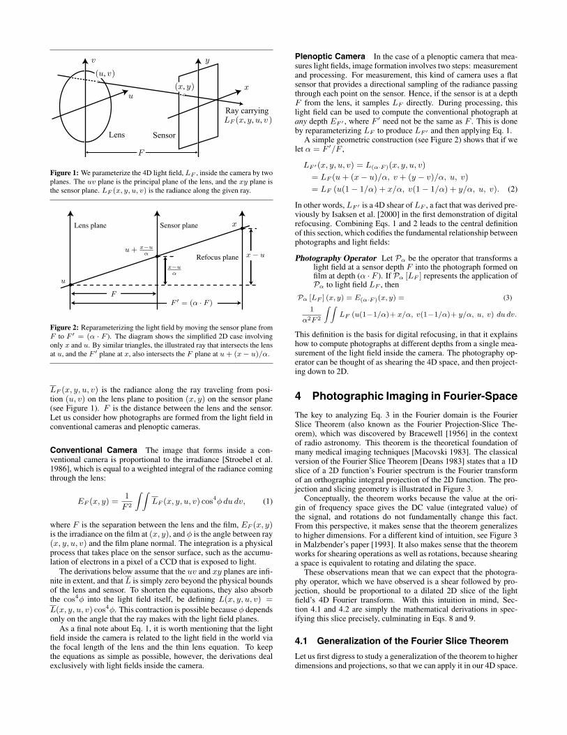
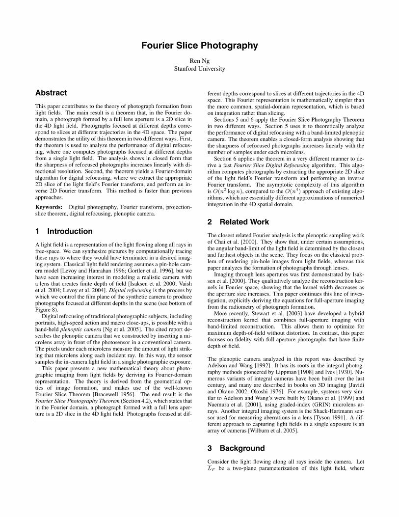
Figure 1: We parameterize the 4D light field, LF , inside the camera by twoplanes. The uv plane is the principal plane of the lens, and the xy plane isthe sensor plane. LF (x, y, u, v) is the radiance along the given ray.

Figure 2: Reparameterizing the light field by moving the sensor plane fromF to F ′ = (α · F ). The diagram shows the simplified 2D case involvingonly x and u. By similar triangles, the illustrated ray that intersects the lensat u, and the F ′ plane at x, also intersects the F plane at u + (x − u)/α.

LF (x, y, u, v) is the radiance along the ray traveling from posi-tion (u, v) on the lens plane to position (x, y) on the sensor plane(see Figure 1). F is the distance between the lens and the sensor.Let us consider how photographs are formed from the light field inconventional cameras and plenoptic cameras.

Conventional Camera The image that forms inside a con-ventional camera is proportional to the irradiance [Stroebel et al.1986], which is equal to a weighted integral of the radiance comingthrough the lens:

EF (x, y) =1

F 2

∫ ∫LF (x, y, u, v) cos4φ du dv, (1)

where F is the separation between the lens and the film, EF (x, y)is the irradiance on the film at (x, y), and φ is the angle between ray(x, y, u, v) and the film plane normal. The integration is a physicalprocess that takes place on the sensor surface, such as the accumu-lation of electrons in a pixel of a CCD that is exposed to light.

The derivations below assume that the uv and xy planes are infi-nite in extent, and that L is simply zero beyond the physical boundsof the lens and sensor. To shorten the equations, they also absorbthe cos4φ into the light field itself, be defining L(x, y, u, v) =

L(x, y, u, v) cos4φ. This contraction is possible because φ dependsonly on the angle that the ray makes with the light field planes.

As a final note about Eq. 1, it is worth mentioning that the lightfield inside the camera is related to the light field in the world viathe focal length of the lens and the thin lens equation. To keepthe equations as simple as possible, however, the derivations dealexclusively with light fields inside the camera.

Plenoptic Camera In the case of a plenoptic camera that mea-sures light fields, image formation involves two steps: measurementand processing. For measurement, this kind of camera uses a flatsensor that provides a directional sampling of the radiance passingthrough each point on the sensor. Hence, if the sensor is at a depthF from the lens, it samples LF directly. During processing, thislight field can be used to compute the conventional photograph atany depth EF ′ , where F ′ need not be the same as F . This is doneby reparameterizing LF to produce LF ′ and then applying Eq. 1.

A simple geometric construction (see Figure 2) shows that if welet α = F ′/F ,

LF ′(x, y, u, v) = L(α·F )(x, y, u, v)

= LF (u + (x − u)/α, v + (y − v)/α, u, v)

= LF (u(1 − 1/α) + x/α, v(1 − 1/α) + y/α, u, v). (2)

In other words, LF ′ is a 4D shear of LF , a fact that was derived pre-viously by Isaksen et al. [2000] in the first demonstration of digitalrefocusing. Combining Eqs. 1 and 2 leads to the central definitionof this section, which codifies the fundamental relationship betweenphotographs and light fields:

Photography Operator Let Pα be the operator that transforms alight field at a sensor depth F into the photograph formed onfilm at depth (α · F ). If Pα [LF ] represents the application ofPα to light field LF , then

Pα [LF ] (x, y) = E(α·F )(x, y) = (3)

1

α2F 2

∫ ∫LF (u(1−1/α)+ x/α, v(1−1/α)+ y/α, u, v) du dv.

This definition is the basis for digital refocusing, in that it explainshow to compute photographs at different depths from a single mea-surement of the light field inside the camera. The photography op-erator can be thought of as shearing the 4D space, and then project-ing down to 2D.

4 Photographic Imaging in Fourier-Space

The key to analyzing Eq. 3 in the Fourier domain is the FourierSlice Theorem (also known as the Fourier Projection-Slice The-orem), which was discovered by Bracewell [1956] in the contextof radio astronomy. This theorem is the theoretical foundation ofmany medical imaging techniques [Macovski 1983]. The classicalversion of the Fourier Slice Theorem [Deans 1983] states that a 1Dslice of a 2D function’s Fourier spectrum is the Fourier transformof an orthographic integral projection of the 2D function. The pro-jection and slicing geometry is illustrated in Figure 3.

Conceptually, the theorem works because the value at the ori-gin of frequency space gives the DC value (integrated value) ofthe signal, and rotations do not fundamentally change this fact.From this perspective, it makes sense that the theorem generalizesto higher dimensions. For a different kind of intuition, see Figure 3in Malzbender’s paper [1993]. It also makes sense that the theoremworks for shearing operations as well as rotations, because shearinga space is equivalent to rotating and dilating the space.

These observations mean that we can expect that the photogra-phy operator, which we have observed is a shear followed by pro-jection, should be proportional to a dilated 2D slice of the lightfield’s 4D Fourier transform. With this intuition in mind, Sec-tion 4.1 and 4.2 are simply the mathematical derivations in spec-ifying this slice precisely, culminating in Eqs. 8 and 9.

4.1 Generalization of the Fourier Slice Theorem

Let us first digress to study a generalization of the theorem to higherdimensions and projections, so that we can apply it in our 4D space.

A closely related generalization is given by the partial Radon trans-form [Liang and Munson 1997], which handles orthographic pro-jections from N dimensions down to M dimensions.

The generalization presented here formulates a broader class ofprojections and slices of a function as canonical projection or slic-ing following an appropriate change of basis (e.g. a 4D shear). Thisapproach is embodied in the following operator definitions.

Integral Projection Let INM be the canonical projection opera-

tor that reduces an N -dimensional function down to M -dimensions by integrating out the last N − M dimensions:IN

M [f ] (x1, . . . , xM ) =∫

f(x1, . . . , xN ) dxM+1 . . . dxN .

Slicing Let SNM be the canonical slicing operator that re-

duces an N -dimensional function down to an M dimen-sional one by zero-ing out the last N − M dimensions:SN

M [f ] (x1, . . . , xM ) = f(x1, . . . , xM , 0, . . . , 0).

Change of Basis Let B denote an operator for an arbitrary changeof basis of an N -dimensional function. It is convenient toalso allow B to act on N -dimensional column vectors as anN×N matrix, so that B [f ] (x) = f(B−1x), where x is anN -dimensional column vector, and B−1 is the inverse of B.

Fourier Transform Let FN denote the N -dimensional Fouriertransform operator, and let F−N be its inverse.

With these definitions, we can state a generalization of the Fourierslice theorem as follows:

THEOREM (GENERALIZED FOURIER SLICE). Let f be an N -dimensional function. If we change the basis of f , integral-projectit down to M of its dimensions, and Fourier transform the resultingfunction, the result is equivalent to Fourier transforming f , chang-ing the basis with the normalized inverse transpose of the originalbasis, and slicing it down to M dimensions. Compactly in terms ofoperators, the theorem says:

FM ◦ INM ◦ B ≡ SN

M ◦ B−T

|B−T | ◦ FN , (4)

where the transpose of the inverse of B is denoted by B−T , and∣∣B−T∣∣ is its scalar determinant.

A proof of the theorem is presented in Appendix A.Figure 4 summarizes the relationships implied by the theorem

between the N -dimensional signal, M -dimensional projected sig-nal, and their Fourier spectra. One point to note about the theoremis that it reduces to the classical version (compare Figures 3 and 4)for N = 2, M = 1 and the change of basis being a 2D rotation ma-trix (B = Rθ). In this case, the rotation matrix is its own inversetranspose (Rθ = Rθ

−T ), and the determinant∣∣Rθ

−T∣∣ equals 1.

The theorem states that when the basis change is not orthonor-mal, then the slice is taken not with the same basis, but rather withthe normalized transpose of the inverse basis, (B−T /

∣∣B−T∣∣). In

2D, this fact is a special case of the so-called Affine Theorem forFourier transforms [Bracewell et al. 1993].

4.2 Fourier Slice Photography

This section derives the equation at the heart of this paper, theFourier Slice Photography Theorem, which factors the Photogra-phy Operator (Eq. 3) using the Generalized Fourier Slice Theo-rem (Eq. 4).

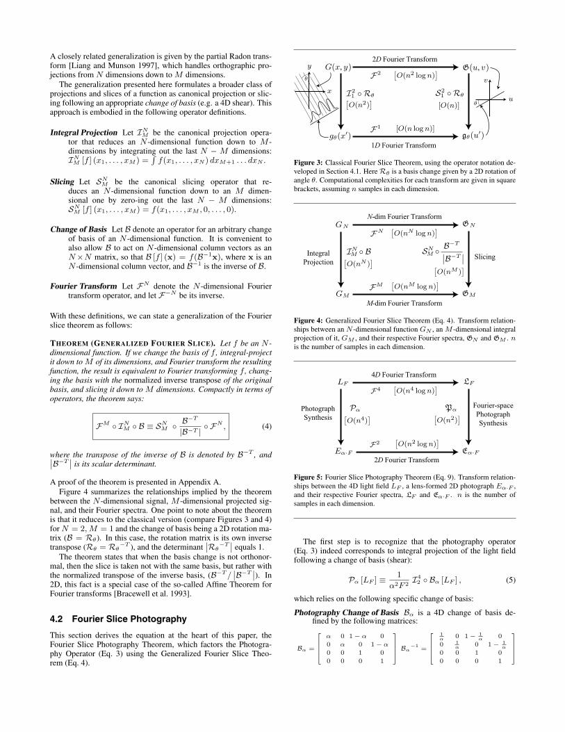
Figure 3: Classical Fourier Slice Theorem, using the operator notation de-veloped in Section 4.1. Here Rθ is a basis change given by a 2D rotation ofangle θ. Computational complexities for each transform are given in squarebrackets, assuming n samples in each dimension.

Figure 4: Generalized Fourier Slice Theorem (Eq. 4). Transform relation-ships between an N -dimensional function GN , an M -dimensional integralprojection of it, GM , and their respective Fourier spectra, GN and GM . nis the number of samples in each dimension.

Figure 5: Fourier Slice Photography Theorem (Eq. 9). Transform relation-ships between the 4D light field LF , a lens-formed 2D photograph Eα·F ,and their respective Fourier spectra, LF and Eα·F . n is the number ofsamples in each dimension.

The first step is to recognize that the photography operator(Eq. 3) indeed corresponds to integral projection of the light fieldfollowing a change of basis (shear):

Pα [LF ] ≡ 1

α2F 2I4

2 ◦ Bα [LF ] , (5)

which relies on the following specific change of basis:

Photography Change of Basis Bα is a 4D change of basis de-fined by the following matrices:

Bα =

α 0 1 − α 0

0 α 0 1 − α

0 0 1 0

0 0 0 1

Bα

−1=

1α 0 1 − 1

α 0

0 1α 0 1 − 1

α

0 0 1 0

0 0 0 1

Directly applying this definition and the definition for I42 verifies

that Eq. 5 is consistent with Eq. 3.We can now apply the Fourier Slice Theorem (Eq. 4) to turn the

integral projection in Eq. 5 into a Fourier-domain slice. Substituting(F−2 ◦S4

2 ◦ (Bα−T /

∣∣Bα−T

∣∣)◦F4) for (I42 ◦Bα), and noting that∣∣Bα

−T∣∣ = 1/α2, we arrive at the following result:

Pα ≡ 1

α2F 2F−2 ◦ S4

2 ◦ Bα−T∣∣Bα−T

∣∣ ) ◦ F4

≡ 1

F 2F−2 ◦ S4

2 ◦ Bα−T ◦ F4 (6)

namely that a lens-formed photograph is obtained from the 4DFourier spectrum of the light field by: extracting an appropriate 2Dslice (S4

2 ◦ Bα−T ), applying an inverse 2D transform (F−2), and

scaling the resulting image (1/F 2).Before stating the final theorem, let us define one last operator

that combines all the action of photographic imaging in the Fourierdomain:

Fourier Photography Operator

Pα ≡ 1

F 2S4

2 ◦ Bα−T . (7)

It is easy to verify that Pα has the following explicit form,directly from the definitions of S4

2 and Bα. This explicit formis required for calculations:

Pα[G](kx, ky) (8)

=1

F 2G(α · kx, α · ky, (1 − α) · kx, (1 − α) · ky).

Applying Eq. 7 to Eq. 6 brings us, finally, to our goal:

THEOREM (FOURIER SLICE PHOTOGRAPHY).

Pα ≡ F−2 ◦ Pα ◦ F4. (9)

A photograph is the inverse 2D Fourier transform of a dilated 2Dslice in the 4D Fourier transform of the light field.

Figure 5 illustrates the relationships implied by this theorem.From an intellectual standpoint, the value of the theorem lies in

the fact that Pα, a slicing operator, is conceptually simpler thanPα, an integral operator. This point is made especially clear by re-viewing the explicit definitions of Pα (Eq. 8) and Pα (Eq. 3). Byproviding a frequency-based interpretation, the theorem contributesinsight by providing two equivalent but very different perspectiveson the physics of image formation. In this regard, the Fourier SlicePhotography Theorem is not unlike the Fourier Convolution The-orem, which provides equivalent but very different perspectives ofconvolution in the two domains.

From a practical standpoint, the theorem provides a faster com-putational pathway for certain kinds of light field processing. Thecomputational complexities for each transform are illustrated inFigure 5, but the main point is that slicing via Pα (O(n2)) isasymptotically faster than integration via Pα (O(n4)). This factis the basis for the algorithm in Section 6.

5 Theoretical Limits of Digital Refocusing

The overarching goal of this section is to demonstrate the theoret-ical utility of the Fourier Slice Photography Theorem. Section 5.1presents a general signal-processing theorem, showing exactly whathappens to photographs when a light field is distorted by a convo-lution filter. Section 5.2 applies this theorem to analyze the perfor-mance of a band-limited light field camera. In these derivations, wewill often use the Fourier Slice Photography Theorem to move theanalysis into the frequency domain, where it becomes simpler.

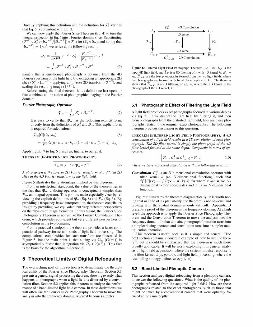
Figure 6: Filtered Light Field Photograph Theorem (Eq. 10). LF is theinput 4D light field, and LF is a 4D filtering of it with 4D kernel k. Eα·Fand Eα·F are the best photographs formed from the two light fields, wherethe photographs are focused with focal plane depth (α · F ). The theoremshows that Eα·F is a 2D filtering of Eα·F , where the 2D kernel is thephotograph of the 4D kernel, k.

5.1 Photographic Effect of Filtering the Light Field

A light field produces exact photographs focused at various depthsvia Eq. 3. If we distort the light field by filtering it, and thenform photographs from the distorted light field, how are these pho-tographs related to the original, exact photographs? The followingtheorem provides the answer to this question.

THEOREM (FILTERED LIGHT FIELD PHOTOGRAPHY). A 4Dconvolution of a light field results in a 2D convolution of each pho-tograph. The 2D filter kernel is simply the photograph of the 4Dfilter kernel focused at the same depth. Compactly in terms of op-erators,

Pα ◦ C4k ≡ C2

Pα[k] ◦ Pα, (10)

where we have expressed convolution with the following operator:

Convolution CNk is an N -dimensional convolution operator with

filter kernel k (an N -dimensional function), such thatCN

k [F ](x) =∫

F (x − u) k(u) du where x and u are N -dimensional vector coordinates and F is an N -dimensionalfunction.

Figure 6 illustrates the theorem diagramatically. It is worth not-ing that in spite of its plausibility, the theorem is not obvious, andproving it in the spatial domain is quite difficult. Appendix Bpresents a proof of the theorem in the frequency-domain. At a highlevel, the approach is to apply the Fourier Slice Photography The-orem and the Convolution Theorem to move the analysis into thefrequency domain. In that domain, photograph formation turns intoa simpler slicing operator, and convolution turns into a simpler mul-tiplication operation.

This theorem is useful because it is simple and general. Thenext section contains a concrete example of how to use the theo-rem, but it should be emphasized that the theorem is much morebroadly applicable. It will be worth exploiting it in general analy-sis of light field acquisition, where the system impulse response isthe filter kernel, k(x, y, u, v), and light field processing, where theresampling strategy defines k(x, y, u, v).

5.2 Band-Limited Plenoptic Camera

This section analyzes digital refocusing from a plenoptic camera,to answer the following questions. What is the quality of the pho-tographs refocused from the acquired light fields? How are thesephotographs related to the exact photographs, such as those thatmight be taken by a conventional camera that were optically fo-cused at the same depth?

The central assumption here, from which we will derive signifi-cant analytical leverage, is that the plenoptic camera captures band-limited light fields. While perfect band-limiting is physically im-possible, it is a plausible approximation in this case because thecamera system blurs the incoming signal through imperfections inits optical elements, through area integration over the physical ex-tent of microlenses and photosensor pixels, and ultimately throughdiffraction.

The band-limited assumption means that the acquired light field,LFL , is a simply the exact light field, LFL , convolved by a perfectlow-pass filter, a 4D sinc:

LFL = C4lowpass [LFL ] , where (11)

lowpass(kx, ky, ku, kv) =

1/(∆x∆u)2 · sinc(kx/∆x, ky/∆x, ku/∆u, kv/∆u). (12)

In this equation, ∆x and ∆u are the linear spatial and direc-tional sampling rates of the integrated light field camera, respec-tively. The 1/(∆x∆u)2 is an energy-normalizing constant toaccount for dilation of the sinc. Also note that, for compact-ness, we use multi-dimensional notation so that sinc(x, y, u, v) =sinc(x) sinc(y) sinc(u) sinc(v).

5.2.1 Analytic Form for Refocused Photographs

Our goal is an analytic solution for the digitally refocused photo-graph, EF , computed from the band-limited light field, LFL . Thisis where we apply the Filtered Light Field Photography Theorem.Letting , α = F/FL,

EF = Pα

[LFL

]= Pα

[C4lowpass [LFL ]

]= C2

Pα[lowpass] [Pα [LFL ]] = C2Pα[lowpass] [EF ] , (13)

where EF is the exact photograph at depth F . This derivationshows that the digitally refocused photograph is a 2D-filtered ver-sion of the exact photograph. The 2D kernel is simply a photographof the 4D sinc function interpreted as a light field, Pα [lowpass].

It turns out that photographs of a 4D sinc light field are simply2D sinc functions:

Pα [lowpass]

= Pα

[1/(∆x∆u)2 · sinc(kx/∆x, ky/∆x, ku/∆u, kv/∆u)

]= 1/D2

x · sinc(kx/Dx, ky/Dx), (14)

where the Nyquist rate of the 2D sinc depends on the amount ofrefocusing, α:

Dx = max(α∆x, |1 − α|∆u). (15)

This fact is difficult to derive in the spatial domain, but applyingthe Fourier Slice Photography Theorem moves the analysis into thefrequency domain, where it is easy (see Appendix C).

The end result here is that, since the 2D kernel is a sinc, theband-limited camera produces digitally refocused photographs thatare just band-limited versions of the exact photographs. The per-formance of digital refocusing is defined by the variation of the 2Dkernel band-width (Eq. 15) with the extent of refocusing.

5.2.2 Interpretation of Refocusing Performance

Notation Recall that the spatial and directional sampling rates ofthe camera are ∆x and ∆u. Let us further define the width ofthe camera sensor as Wx, and the width of the lens aperture asWu. With these definitions, the spatial resolution of the sensorsis Nx = Wx/∆x and the directional resolution of the light fieldcamera is Nu = Wu/∆u.

Exact Refocusing Since α = (F/FL) and ∆u = Wu/Nu, it iseasy to verify that

|α∆x| ≥ |(1 − α)∆u|⇔ |F − FL| ≤ ∆x(NuF/Wu). (16)

The claim here is that this is the range of focal depths, FL, wherewe can achieve “exact” refocusing, i.e. compute a sharp renderingof the photograph focused at that depth. What we are interestedin is the Nyquist-limited resolution of the photograph, which is thenumber of band-limited samples within the field of view.

Precisely, by applying Eq. 16 to Eq. 15, we see that the band-width of the computed photograph is (α∆x). Next, the field ofview is not simply the size of the light field sensor, Wx, but rather(αWx). This dilation is due to the fact that digital refocusing scalesthe image captured on the sensor by a factor of α in projecting itonto the refocus focal plane (see Eq. 3). If α > 1, for example,the light field camera image is zoomed in slightly compared to theconventional camera. Figure 7 illustrates this effect.

Thus, the Nyquist resolution of the computed photograph is

(αWx)/(α∆x) = Wx/∆x. (17)

This is simply the spatial resolution of the camera, the maximumpossible resolution for the output photograph. This justifies the as-sertion that the refocusing is “exact” for the range of depths definedby Eq. 16. Note that this range of exact refocusing increases lin-early with the directional resolution, Nu.

Inexact Refocusing If we exceed the exact refocusing range, i.e.

|F − FL| > ∆x(NuF/Wu). (18)

then the band-limit of the computed photograph, EF , is|1 − α|∆u > α∆x (see Eq. 15), and the resulting resolution isnot maximal, but rather (αWx)/(|1 − α|∆u), which is less thanWx/∆x. In other words, the resulting photograph is blurred, withreduced Nyquist-limited resolution.

Re-writing this resolution in a slightly different form providesa more intuitive interpretation of the amount of blur. Since α =F/FL and ∆u = Wu/Nu, the resolution is

αWx

|1 − α|∆u=

Wx

Wu/(Nu · F ) · |F − FL| . (19)

Since ((NuF )/Wu) is the f -number of a lens Nu times smallerthan the actual lens used on the camera, we can now interpretWu/(Nu · F ) · |F − FL| as the size of the conventional circle ofconfusion cast through this smaller lens when the film plane is mis-focused by a distance of |F − FL|.

In other words, when refocusing beyond the exact range, we canonly make the desired focal plane appear as sharp as it appears in aconventional photograph focused at the original depth, with a lensNu times smaller. Note that the sharpness increases linearly withthe directional resolution, Nu.

5.3 Summary

It is worth summarizing the point of the analysis in Section 5. Ona meta-level, this section has demonstrated the theoretical utility ofthe Fourier Slice Photography Theorem, applying it several timesin deriving Eqs. 10, 13 and 14.

At another level, this section has derived two end results that areof some importance. The first is the Filtered Light Field Photogra-phy Theorem, which is a simple but general signal-processing toolfor analyzing light field imaging systems. The second is the fact thatmaking a simple band-limited assumption about plenoptic cameras

Sensor Depth Conventional Plenoptic

α = 0.82

Inexactrefocusing

α = 0.90

Exactrefocusing

α = 1.0

α = 1.11

Exactrefocusing

α = 1.25

Inexactrefocusing

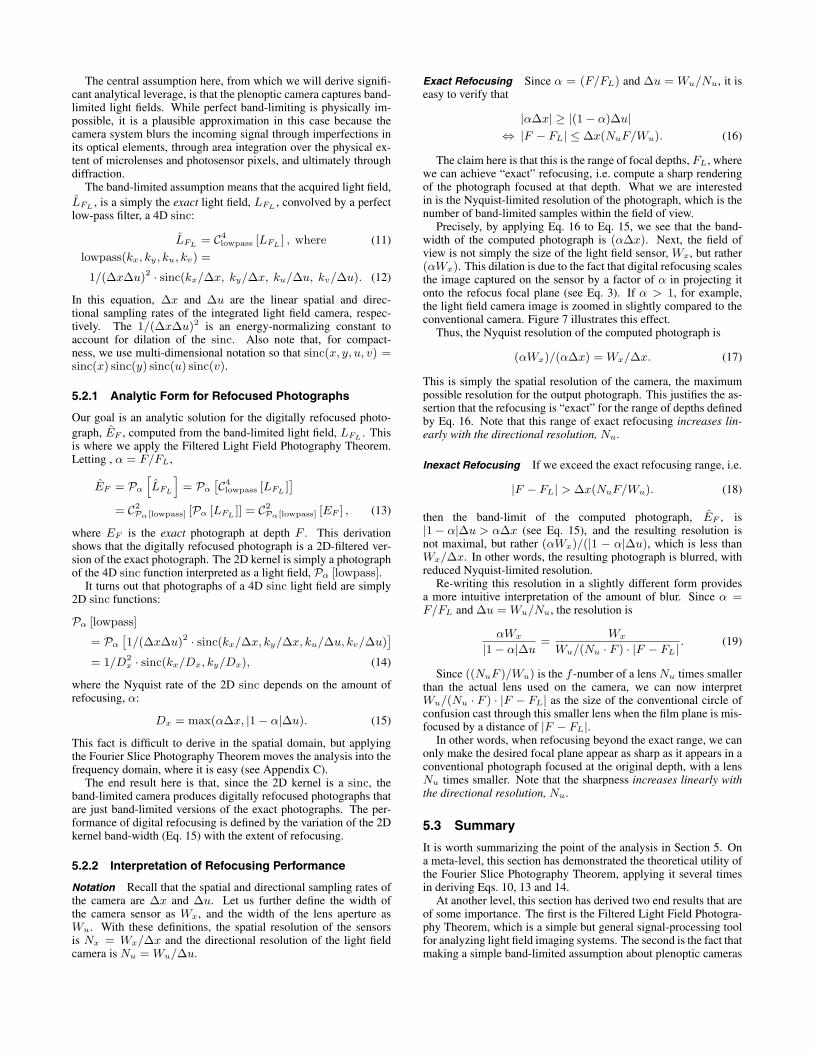
Figure 7: Photographs produced by an f/4 conventional and an f/4plenoptic [Ng et al. 2005] camera, using digital refocusing (via Eq. 3) inthe latter case. The sensor depth is given as a fraction of the film depth thatbrings the target into focus. Note that minor refocusing provides the plenop-tic camera with a wider effective depth of focus than the conventional sys-tem. Also note how the field of view changes slightly with the sensor depth,a change due to divergence of the light rays from the lens aperture.

yields an analytic proof that limits on digital refocusing improvelinearly with directional resolution. Experiments with the plenopticcamera that we built achieved refocusing performance within a fac-tor of 2 of this theory [Ng et al. 2005]. With Nu = 12, this enablessharp refocusing of f/4 photographs within the wide depth of fieldof an f/22 aperture.

6 Fourier Slice Digital Refocusing

This section applies the Fourier Slice Photography Theorem in avery different way, to derive an asymptotically fast algorithm fordigital refocusing. The presumed usage scenario is as follows: anin-camera light field is available (perhaps having been captured by aplenoptic camera). The user wishes to digitally refocus in an inter-active manner, i.e. select a desired focal plane and view a syntheticphotograph focused on that plane (see bottom row of Figure 8).

In previous approaches to this problem [Isaksen et al. 2000;Levoy et al. 2004; Ng et al. 2005], spatial integration via Eq. 3results in an O(n4) algorithm, where n is the number of samples ineach of the four dimensions. The algorithm described in this sec-tion provides a faster O(n2 log n) algorithm, with the penalty of asingle O(n4 log n) pre-processing step.

6.1 Algorithm

The algorithm follows trivially from the Fourier Slice PhotographyTheorem:

Preprocess Prepare the given light field, LF , by pre-computing its4D Fourier transform, F4 [L], via the Fast Fourier Transform.This step takes O(n4 log n) time.

Refocusing For each choice of desired world focus plane, W ,

• Compute the conjugate virtual film plane depth, F ′, via thethin lens equation: 1/F ′ + 1/W = 1/f , where f is the focallength of the lens.

• Extract the dilated Fourier slice (via Eq. 8) of the pre-processed Fourier transform, to obtain (Pα ◦ F4) [L], whereα = F ′/F . This step takes O(n2) time.

• Compute the inverse 2D Fourier transform of the slice, to ob-tain (F−2 ◦Pα ◦ F4) [L]. By the theorem, this final result isPα [LF ] = EF ′ the photo focused on world plane W . Thisstep takes O(n2 log n) time.

Figure 8 illustrates the steps of the algorithm.

6.2 Implementation and Results

The complexity in implementing this simple algorithm has to dowith ameliorating the artifacts that result from discretization, re-sampling and Fourier transformation. These artifacts are concep-tually the same as the artifacts tackled in Fourier volume render-ing [Levoy 1992; Malzbender 1993], and Fourier-based medicalreconstruction techniques [Jackson et al. 1991] such as those usedin CT and MR. The interested reader should consult these citationsand their bibliographies for further details.

6.2.1 Sources of Artifacts

In general signal-processing terms, when we sample a signal it isreplicated periodically in the dual domain. When we reconstructthis sampled signal with convolution, it is multiplied in the dualdomain by the Fourier transform of the convolution filter. The goalis to perfectly isolate the original, central replica, eliminating allother replicas. This means that the ideal filter is band-limited: it isof unit value for frequencies within the support of the light field,and zero for all other frequencies. Thus, the ideal filter is the sincfunction, which has infinite extent.

In practice we must use an imperfect, finite-extent filter, whichwill exhibit two important defects (see Figure 9). First, the filterwill not be of unit value within the band-limit, gradually decayingto smaller fractional values as the frequency increases. Second, thefilter will not be truly band-limited, containing energy at frequen-cies outside the desired stop-band.

The first defect leads to so-called rolloff artifacts [Jackson et al.1991], the most obvious manifestation of which is a darkening ofthe borders of computed photographs (see Figure 10). Decay in thefilter’s frequency spectrum with increasing frequency means thatthe spatial light field values, which are modulated by this spectrum,also “roll off” to fractional values towards the edges.

The second defect, energy at frequencies above the band-limit,leads to aliasing artifacts (postaliasing, in the terminology of

����F4

����Pα>1

����Pα=1

����Pα<1

����F−2

����F−2

����F−2

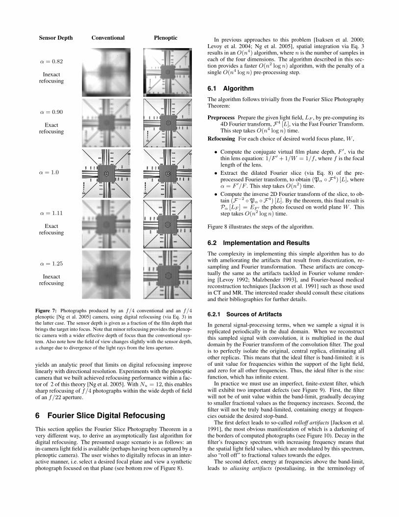
Figure 8: Fourier Slice Digital Refocusing algorithm. Row 1: 4D light fieldcaptured from a plenoptic camera, with four close-ups. Row 2: 4D Fouriertransform of the light field, with four close-ups. Row 3: Three 2D slices ofthe 4D Fourier transform, extracted by Pα (Eq. 8) with different values ofα. Row 4: Inverse 2D transforms of row 3. These images are conventionalphotographs focused on the closest, middle and furthest crayons. Row 5:Same images as row 4 except computed with brute-force integration in thespatial domain via Eq. 3, for comparison.

Mitchell and Netravali [1998]) in computed photographs (see Fig-ure 10). The non-zero energy beyond the band-limit means that theperiodic replicas are not fully eliminated, leading to two kinds ofaliasing. First, the replicas that appear parallel to the slicing planeappear as 2D replicas of the image encroaching on the borders ofthe final photograph. Second, the replicas positioned perpendicu-lar to this plane are projected and summed onto the image plane,creating ghosting and loss of contrast.

6.2.2 Correcting Rolloff Error

Rolloff error is a well understood effect in medical imaging andFourier volume rendering. The standard solution is to multiply theaffected signal by the reciprocal of the filter’s inverse Fourier spec-trum, to nullify the effect introduced during resampling. In ourcase, directly analogously to Fourier volume rendering [Malzben-der 1993], the solution is to spatially pre-multiply the input lightfield by the reciprocal of the filter’s 4D inverse Fourier transform(see Figure 11). This is performed prior to taking its 4D Fouriertransform in the pre-processing step of the algorithm.

Unfortunately, this pre-multiplication tends to accentuate the en-ergy of the light field near its borders, maximizing the energy thatfolds back into the desired field of view as aliasing.

6.2.3 Suppressing Aliasing Artifacts

The three main methods of suppressing aliasing artifacts areoversampling, superior filtering and zero-padding. Oversamplingwithin the extracted 2D Fourier slice (PF ◦ F4) [L] increases thereplication period in the spatial domain. This means that less en-ergy in the tails of the in-plane replicas will fall within the bordersof the final photograph.

Exactly what happens computationally will be familiar to thoseexperienced in discrete Fourier transforms. Specifically, increasingthe sampling rate in one domain leads to an increase in the field ofview in the other domain. Hence, by oversampling we produce animage that shows us more of the world than desired (see Figure 12),not a magnified view of the desired portion. Aliasing energy fromneighboring replicas falls into these outer regions, which we cropaway to isolate the central image of interest.

Oversampling is appealing because of its simplicity, but over-sampling alone cannot produce good quality images. The problemis that it cannot eliminate the replicas that appear perpendicular tothe slicing plane, which are projected down onto the final image asdescribed in the previous section.

This brings us to the second major technique of combating alias-ing: superior filtering. As already stated, the ideal filter is a sincfunction with a band-limit matching the spatial bounds of the lightfield. Our goal is to use a finite-extent filter that approximatesthis perfect spectrum as closely as possible. The best methods forproducing such filters use iterative techniques to jointly optimizethe band-limit and narrow spatial support, as described in Jack-son et al. [1991] in the medical imaging community, and Malzben-der [1993] in the Fourier volume rendering community.

Jackson et al. show that a much simpler, and near-optimal, ap-proximation is the Kaiser-Bessel function. They also provide opti-mal Kaiser-Bessel parameter values for minimizing aliasing. Fig-ure 13 illustrates the striking reduction in aliasing provided by suchoptimized Kaiser-Bessel filters compared to inferior quadrilinearinterpolation. Surprisingly, a Kaiser-Bessel window of just width2.5 suffices for excellent results.

The third and final method to combat aliasing is to pad the lightfield with a small border of zero values before pre-multiplicationand taking its Fourier transform [Levoy 1992; Malzbender 1993].This pushes energy slightly further from the borders, and minimizesthe amplification of aliasing energy by the pre-multiplication de-scribed in 6.2.2.

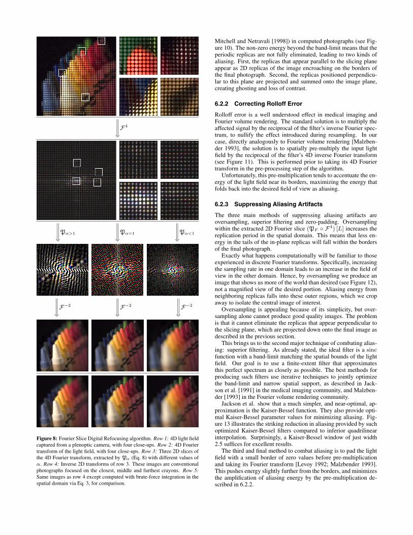
Figure 9: Source of artifacts. Left: Triangle reconstruction filter. Right:Frequency spectrum of this filter (solid line) compared to ideal spectrum(dotted line). Shaded regions show deviations that lead to artifacts.

Figure 10: Two main classes of artifacts. Left: Gold-standard image pro-duced by spatial integration via Eq. 3. Middle: Rolloff artifacts usingKaiser-Bessel filter. Right: Aliasing artifacts using quadrilinear filter.

Figure 11: Rolloff correction by pre-multiplying the input light field by thereciprocal of the resmpling filter’s inverse Fourier transform. Left: Kaiser-Bessel filtering without pre-multiplication. Right: With pre-multiplication.

Figure 12: Aliasing reduction by oversampling. Quadrilinear filter used toemphasize aliasing effects for didactic purposes. Top left pair: 2D Fourierslice and inverse-transformed photograph, with unit sampling. Bottom:Same as top left pair, except with 2× oversampling in the frequency do-main. Top right: Cropped version of bottom right. Note that aliasing isreduced compared to version with unit sampling.

Figure 13: Aliasing reduction by superior filtering. Rolloff correction isapplied. Left: Quadrilinear filter (width 2). Middle: Kaiser-Bessel filter,width 1.5. Right: Kaiser-Bessel filter, width 2.5.

6.2.4 Implementation Summary

We directly discretize the algorithm presented in 6.1, applying thefollowing four techniques (from 6.2.2 and 6.2.3) to suppress arti-facts. In the pre-processing phase,

1. We pad the light field with a small border (5% of the width inthat dimension) of zero values.

2. We pre-multiply the light field by the reciprocal of the Fouriertransform of the resampling filter.

In the refocusing step where we extract the 2D Fourier slice,

3. We use a linearly-separable Kaiser-Bessel resampling filter.width 2.5 produces excellent results. For fast previewing, anextremely narrow filter of width 1.5 produces results that aresuperior to (and faster than) quadrilinear interpolation.

4. We oversample the 2D Fourier slice by a factor of 2. AfterFourier inversion, we crop the resulting photograph to isolatethe central quadrant.

The bottom two rows of Figure 8 compare this implementationof the Fourier Slice algorithm with spatial integration.

6.2.5 Performance Summary

This section compares the performance of our algorithm comparedto spatial-domain methods. Tests were performed on a 3.0 GhzPentium IV processor. The FFTW-3 library [Frigo and Johnson1998] was used to compute Fourier transforms efficiently.

For a light field with 256×256 st resolution and 16×16 uv resolu-tion, spatial-domain integration achieved 1.68 fps (frames per sec-ond) using nearest-neighbor quadrature and 0.13 fps using quadri-linear interpolation. In contrast, the Fourier Slice method presentedin this paper achieved 2.84 fps for previewing (Kaiser-Bessel fil-ter, width 1.5 and no oversampling) and 0.54 fps for higher quality(width 2.5 and 2x oversampling). At these resolutions, performancebetween spatial-domain and Fourier-domain methods are compara-ble. The pre-processing time, however, was 47 seconds.

The Fourier Slice method outperforms the spatial methods as thedirectional uv resolution increases, because the number of lightfield samples that must be summed increases for the spatial inte-gration methods, but the cost of slicing stays constant per pixel.For a light field with 128×128 st resolution and 32×32 uv reso-lution, spatial-domain integration achieved 1.63 fps using nearest-neighbor, and 0.10 fps using quadrilinear interpolation. The FourierSlice method achieved 15.58 fps for previewing and 2.73 fps forhigher quality. At these resolutions, the Fourier slice methods arean order of magnitude faster. In this case, the pre-processing timewas 30 seconds.

7 Conclusions and Future Work

The main contribution of this paper is the Fourier Slice Photogra-phy Theorem. By describing how photographic imaging occurs inthe Fourier domain, this simple but fundamental result provides aversatile tool for algorithm development and analysis of light fieldimaging systems. This paper tries to present concrete examples ofthis utility in analyzing a band-limited plenoptic camera, and in de-veloping the Fourier Slice Digital Refocusing algorithm.

The band-limited analysis provides theoretical backing for recentexperimental results demonstrating exciting performance of digi-tal refocusing from plenoptic camera data [Ng et al. 2005]. Thederivations also yield a general-purpose tool (Eq. 10) for analyzingplenoptic camera systems.

The Fourier Slice Digital Refocusing algorithm is asymptoticallyfaster than previous approaches. It is also efficient in a practicalsense, thanks to the optimized Kaiser-Bessel resampling strategyborrowed directly from the tomography literature. Continuing toexploit this connection with tomography will surely yield furtherbenefits in light field processing.

A clear line of future work would extend the algorithm to in-crease its focusing flexibility. Presented here in its simplest form,the algorithm is limited to full-aperture refocusing. Support for dif-ferent apertures could be provided by appropriate convolution inthe Fourier domain that results in a spatial multiplication maskingout the undesired portion of the aperture. This is related to work inFourier volume shading [Levoy 1992].

A very different class of future work might emerge from lookingat the footprint of photographs in the 4D Fourier transform of thelight field. It is a direct consequence of the Fourier Slice Photog-raphy Theorem (consider Eq. 9 for all α) that the footprint of allfull-aperture photographs lies on the following 3D manifold in the4D Fourier space:

{(α · kx, α · ky, (1 − α) · kx, (1 − α) · ky)

where α ∈ [0,∞), and kx, ky ∈ R}

(20)

Two possible lines of research are as follows.First, it might be possible to optimize light field camera designs

to provide greater fidelity on this manifold, at the expense of thevast remainder of the space that does not contribute to refocusedphotographs. One could also compress light fields for refocusingby storing only the data on the 3D manifold.

Second, photographs focused at a particular depth will containsharp details (hence high frequencies) only if an object exists at thatdepth. This observation suggests a simple Fourier Range Findingalgorithm: search for regions of high spectral energy on the 3Dmanifold at a large distance from the origin. The rotation angleof these regions gives the depth (via the Fourier Slice PhotographyTheorem) of focal planes that intersect features in the visual world.

Acknowledgments

Thanks to Marc Levoy, Pat Hanrahan, Ravi Ramamoorthi, MarkHorowitz, Brian Curless and Kayvon Fatahalian for discussions,help with references and reading a draft. Marc Levoy took the pho-tograph of the crayons. Thanks also to Dwight Nishimura and BradOsgood. Finally, thanks to the anonymous reviewers for their help-ful feedback and comments. This work was supported by NSF grant0085864-2 (Interacting with the Visual World), and by a MicrosoftResearch Fellowship.

ReferencesADELSON, T., AND WANG, J. Y. A. 1992. Single lens stereo with a

plenoptic camera. IEEE Transactions on Pattern Analysis and MachineIntelligence 14, 2 (Feb), 99–106.

BRACEWELL, R. N., CHANG, K.-Y., JHA, A. K., AND WANG, Y. H.1993. Affine theorem for two-dimensional fourier transform. ElectronicsLetters 29, 304–309.

BRACEWELL, R. N. 1956. Strip integration in radio astronomy. Aust. J.Phys. 9, 198–217.

BRACEWELL, R. N. 1986. The Fourier Transform and Its Applications,2nd Edition Revised. WCB / McGraw-Hill.

CHAI, J., TONG, X., AND SHUM, H. 2000. Plenoptic sampling. In SIG-GRAPH 00, 307–318.

DEANS, S. R. 1983. The Radon Transform and Some of Its Applications.Wiley-Interscience.

FRIGO, M., AND JOHNSON, S. G. 1998. FFTW: An adaptive softwarearchitecture for the FFT. In ICASSP conference proceedings, vol. 3,1381–1384.

GORTLER, S. J., GRZESZCZUK, R., SZELISKI, R., AND COHEN, M. F.1996. The Lumigraph. In SIGGRAPH 96, 43–54.

ISAKSEN, A., MCMILLAN, L., AND GORTLER, S. J. 2000. Dynamicallyreparameterized light fields. In SIGGRAPH 2000, 297–306.

IVES, H. E. 1930. Parallax panoramagrams made with a large diameterlens. J. Opt. Soc. Amer. 20, 332–342.

JACKSON, J. I., MEYER, C. H., NISHIMURA, D. G., AND MACOVSKI,A. 1991. Selection of convolution function for fourier inversion usinggridding. IEEE Transactions on Medical Imaging 10, 3, 473–478.

JAVIDI, B., AND OKANO, F., Eds. 2002. Three-Dimensional Television,Video and Display Technologies. Springer-Verlag.

LEVOY, M., AND HANRAHAN, P. 1996. Light field rendering. In SIG-GRAPH 96, 31–42.

LEVOY, M., CHEN, B., VAISH, V., HOROWITZ, M., MCDOWALL, I.,AND BOLAS, M. 2004. Synthetic aperture confocal imaging. ACMTransactions on Graphics 23, 3, 822–831.

LEVOY, M. 1992. Volume rendering using the fourier projection-slice the-orem. In Proceedings of Graphics Interface ’92, 61–69.

LIANG, Z.-P., AND MUNSON, D. C. 1997. Partial Radon transforms. IEEETransactions on Image Processing 6, 10 (Oct 1997), 1467–1469.

LIPPMANN, G. 1908. La photographie integrale. Comptes-Rendus,Academie des Sciences 146, 446–551.

MACOVSKI, A. 1983. Medical Imaging Systems. Prentice Hall.

MALZBENDER, T. 1993. Fourier volume rendering. ACM Transactions onGraphics 12, 3, 233–250.

MITCHELL, D. P., AND NETRAVALI, A. N. 1998. Reconstruction filtersin computer graphics. In SIGGRAPH 98, 221–228.

NAEMURA, T., YOSHIDA, T., AND HARASHIMA, H. 2001. 3-D computergraphics based on integral photography. Optics Express 8, 2, 255–262.

NG, R., LEVOY, M., BREDIF, M., DUVAL, G., HOROWITZ, M., AND

HANRAHAN, P. 2005. Light field photography with a hand-held plenop-tic camera. Tech. Rep. CSTR 2005-02, Stanford Computer Science.http://graphics.stanford.edu/papers/lfcamera.

OKANO, F., ARAI, J., HOSHINO, H., AND YUYAMA, I. 1999. Three-dimensional video system based on integral photography. Optical Engi-neering 38, 6 (June 1999), 1072–1077.

OKOSHI, T. 1976. Three-Dimensional Imaging Techniques. Acad. Press.

STEWART, J., YU, J., GORTLER, S. J., AND MCMILLAN, L. 2003. A newreconstruction filter for undersampled light fields. In Proceedings of theEurographics Symposium on Rendering 2003, 150 – 156.

STROEBEL, L., COMPTON, J., CURRENT, I., AND ZAKIA, R. 1986. Pho-tographic Materials and Processes. Focal Press.

TYSON, R. K. 1991. Principles of Adaptive Optics. Academic Press.

VAISH, V., WILBURN, B., JOSHI, N., AND LEVOY, M. 2004. Using plane+ parallax for calibrating dense camera arrays. In Proc. of CVPR, 2–9.

WILBURN, B., JOSHI, N., VAISH, V., TALVALA, E.-V., ANTUNEZ, E.,BARTH, A., ADAMS, A., LEVOY, M., AND HOROWITZ, M. 2005.High performance imaging using large camera arrays. To appear at SIG-GRAPH 2005.

Appendices: Proofs and Derivations

A Generalized Fourier Slice Theorem

Theorem (Generalized Fourier Slice).

FM ◦ INM ◦ B ≡ SN

M ◦(B−T /

∣∣∣B−T∣∣∣)◦ FN

Proof. The following proof is inspired by one common approachto proving the classical 2D version of the theorem. The first step isto note that

FM ◦ INM = SN

M ◦ FN , (21)

because substitution of the basic definitions shows that for anarbitrary function, f , both (FM ◦ IN

M ) [f ] (u1, . . . , uM ) and(SN

M ◦ FN ) [f ] (u1, . . . , uM ) are equal to∫f(x1, . . . , xN ) exp (−2πi (x1u1 + · · · + xMuM )) dx1 . . . dxN .

The next step is to observe that if basis change operators commutewith Fourier transforms via FN ◦ B ≡ (B−T /

∣∣B−T∣∣) ◦ FN , then

the proof of the theorem would be complete because for every func-tion f we would have

(FM ◦ INM ◦ B) [f ] = (SN

M ◦ FN ) [B [f ]] (by Eq. 21)

=(SN

M ◦(B−T /

∣∣∣B−T∣∣∣)◦ FN

)[f ] . (commute) (22)

Thus, the final step is to show that FN ◦ B ≡ (B−T /∣∣B−T

∣∣) ◦FN . Directly substituting the operator definitions establishes thesetwo equations:

(B ◦ FN ) [f ] (u) =

∫f(x) exp

(−2πi

(xT

(B−1u)))

dx; (23)

(FN◦ B−T

|B−T |)

[f ] (u) (24)

=1

|B−T |∫

f(BT x′

)exp

(−2πi(x′ · u))

dx′.

In these equations, x and u are N -dimensional column vectors, andthe integral is taken over all of N -dimensional space.

Let us now apply the change of variables x = BT x′ to Eq. 24,noting that x′ = B−T x, and dx =

(1/

∣∣B−T∣∣) dx. Making these

substitutions,(FN◦ B−T

|B−T |)

[f ] (u) =

∫f (x) exp

(−2πi

((B−T x

)Tu

))dx

=

∫f (x) exp

(−2πi

(xTB−1u

))dx

(25)

where the last line relies on the linear algebra rule for trans-posing matrix products. Equations 23 and 25 show thatFN ◦ B ≡ (B−T /

∣∣B−T∣∣) ◦ FN , completing the proof.

B Filtered Light Field Photography Thm.

Theorem (Filtered Light Field Photography).

PF ◦ C4k ≡ C2

PF [k] ◦ PF ,

To prove the theorem, let us first establish a lemma involving theclosely-related modulation operator:

Modulation MNβ is an N -dimensional modulation operator, such

that MNβ [F ] (x) = F (x)·β(x) where x is an N -dimensional

vector coordinate.

Lemma. Multiplying an input 4D function by another one, k, andtransforming the result by PF , the Fourier photography operator,is equivalent to transforming both functions by PF and then multi-plying the resulting 2D functions. In operators,

PF ◦M4k ≡ M2

PF [k] ◦ PF (26)

Algebraic verification of the lemma is direct given the basic def-initions, and is omitted here. On an intuitive level, however, thelemma makes sense because Pα is a slicing operator: multiplyingtwo functions and then slicing them is the same as slicing each ofthem and multiplying the resulting functions.

Proof of theorem. The first step is to translate the classical FourierConvolution Theorem (see, for example, Bracewell [1986]) intouseful operator identities. The Convolution Theorem states that amultiplication in the spatial domain is equivalent to convolution inthe Fourier domain, and vice versa. As a result,

FN ◦ CNk ≡ MN

FN [k] ◦ FN (27)

and FN ◦MNk ≡ CN

FN [k] ◦ FN . (28)

Note that these equations also hold for negative N , since the Con-volution Theorem also applies to the inverse Fourier transform.

With these facts and the lemma in hand, the proof of the theoremproceeds swiftly:

PF ◦ C4k ≡ F−2 ◦ PF ◦ F4 ◦ C4

k

≡ F−2 ◦ PF ◦M4F4[k]

◦ F4

≡ F−2 ◦M2(PF ◦F4)[k]

◦ PF ◦ F4

≡ C2(F−2◦PF ◦F4)[k]

◦ F−2 ◦ PF ◦ F4

≡ C2PF [k] ◦ PF ,

where we apply the Fourier Slice Photography Theorem (Eq. 9) toderive the first and last lines, the Convolution Theorem (Eqs. 27and 28) for the second and fourth lines, and the lemma (Eq. 26) forthe third line.

C Photograph of a 4D Sinc Light Field

This appendix derives Eq. 14, which states that a photo from a 4Dsinc light field is a 2D sinc function. The first step is to apply theFourer Slice Photography Theorem to move the derivation into theFourier domain.Pα

[1/(∆x∆u)2 · sinc(x/∆x, y/∆x, u/∆u, v/∆u)

]=1/(∆x∆u)2 · (F−2 ◦ Pα ◦ F4) [sinc(x/∆x, y/∆x, u/∆u, v/∆u)]

=(F−2 ◦ Pα) [�(kx∆x, ky∆x, ku∆u, kv∆u)] . (29)

Now we apply the definition for the Fourier photography operatorPα (Eq. 7), to arrive at

Pα

[1/(∆x∆u)2 · sinc(x/∆x, y/∆x, u/∆u, v/∆u)

](30)

= F−2 [�(αkx∆x, αky∆x, (1 − α)kx∆u, (1 − α)ky∆u)] .

Note that the 4D rect function now depends only on kx and ky , notku or kv . Since the product of two dilated rect functions is equal tothe smaller rect function,

Pα

[1/(∆x∆u)2 · sinc(x/∆x, y/∆x, u/∆u, v/∆u)

]= F−2 [�(kxDx, kyDx)] (31)

where Dx = max(α∆x, |1 − α|∆u). (32)

Applying the inverse 2D Fourier transform completes the proof:

Pα

[1/(∆x∆u)2 · sinc(x/∆x, y/∆x, u/∆u, v/∆u)

]= 1/D2

x · sinc(kx/Dx, ky/Dx). (33)