Embed Size (px)
Citation preview
Chapter 3
Fourier Series
3.1 Some Properties of Functions
3.1.1 Goal
We review some results about functions which play an important role in thedevelopment of the theory of Fourier series. These results will be needed for theremaining sections. We also introduce some notation.
3.1.2 Preliminary Remarks
Joseph Fourier (1768-1830) who gave his name to Fourier series, was not the firstto use Fourier series neither did he answer all the questions about them. Theseseries had already been studied by Euler, d’Alembert, Bernoulli and others be-fore him. Fourier also thought wrongly that any function could be representedby Fourier series. However, these series bear his name because he studied themextensively. The first concise study of these series appeared in Fourier’s publica-tions in 1807, 1811 and 1822 in his Théorie analytique de la chaleur. He appliedthe technique of Fourier series to solve the heat equation. He had the insightto see the power of this new method. His work set the path for techniques thatcontinue to be developed even today.Fourier Series, like Taylor series, are special types of expansion of functions.
With Taylor series, we are interested in expanding a function in terms of thespecial set of functions 1, x, x2, x3, ... or more generally in terms of 1, (x− a),(x− a)
2, (x− a)3, .... You will remember from calculus that if a function f has
a power series representation at a then
f (x) =
∞∑n=0
f (n) (a)
n!(x− a)
n (3.1)
Remember from calculus that a series is an infinite sum. We never use the full se-
117
118 CHAPTER 3. FOURIER SERIES
ries, we usually truncate it. In other words, if we call SN (x) =
N∑n=0
f (n) (a)
n!(x− a)
n,
then we approximate f (x) by Sn (x). Sn (x) is called a partial sum. A reasonfor using Taylor series is that their partial sums are polynomials and polynomialsare the easiest functions to work with.With Fourier series, we are interested in expanding a function f in terms
of the special set of functions 1, cosπx
L, cos
2πx
L, cos
3πx
L, ..., sin
πx
L, sin
2πx
L,
sin3πx
L, ... Thus, a Fourier series expansion of a function is an expression of the
form
f (x) = A0 +
∞∑n=1
(An cos
nπx
L+Bn sin
nπx
L
)for some positive constant L. In the previous chapters, we saw this was usefulin helping us to solve certain PDEs. Another reason for using Fourier series isif f (x) represents some signal (light, sound) since signals are a combination ofperiodic functions. So it is natural we might want to write f (x) as a Fourierseries.However, there are several questions which arise when trying to achieve this.
We list them here and will try to answer most of them in this chapter. It isimportant for the reader to be aware of these questions.
1. Given a function f (x), how do we know if it has a Fourier seriesrepresentation? Fourier thought every function did. It turns out it isnot quite the case, though many functions do.
2. Given a function f (x) which has a Fourier series representation,how do we find the coeffi cients An and Bn? We have already an-swered this question in the previous chapters.
3. Infinite series do not always converge. Some converge for some values of xand not for others. Does the Fourier series converge and for whichvalues of x?
4. Even if the Fourier series of a function f converges, does it con-verge to f (x)? We will see that even if a Fourier series converges, it doesnot always converge to f (x).
5. Since a Fourier series is an infinite sum, the sum rules we know for deriv-atives and integrals do not apply here. In other words, how do wedifferentiate and integrate a Fourier series? Can we differentiateand integrate a Fourier series term by term? We assumed we could in theprevious chapter, but we do not know that. Though we will see it is truefor most functions, it is not always true.
6. Given an initial boundary value problem (IBVP), is the resultingFourier series really a solution of the IBVP? Keep in mind that to
3.1. SOME PROPERTIES OF FUNCTIONS 119
check this, we will have to differentiate the Fourier series, hence the answerto the previous question is relevant.
After reviewing some properties of functions, we will review how to representa function by its Fourier series. We will then answer the question listed above.We will finish these notes by discussing some applications of Fourier series.
3.1.3 Even, Odd Functions
Definition 106 (Even and Odd) Let f be a function defined on an intervalI (finite or infinite) centered at x = 0.
1. f is said to be even if f (−x) = f (x) for every x in I.
2. f is said to be odd if f (−x) = −f (x) for every x in I.
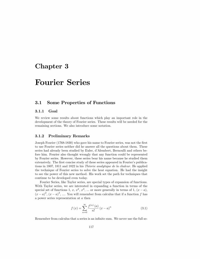
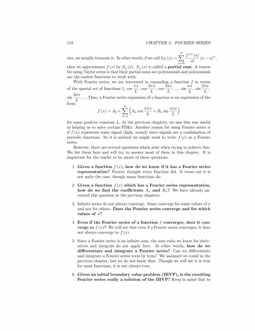
The graph of an even function is symmetric with respect to the y-axis. Thegraph of an odd function is symmetric with respect to the origin.
Example 107 1, x2, xn (where n is even), and cosx are all even functions
Example 108 x, x3, xn (where n is odd), and sinx are all odd functions.
You will recall from calculus the following important theorem about inte-grating even and odd functions over an interval of the form [−a, a] where a > 0.
Theorem 109 Let f be a function which domain includes [−a, a] where a > 0.
1. If f is even, then∫ a−a f (x) dx = 2
∫ a0f (x) dx
2. If f is odd, then∫ a−a f (x) dx = 0
There are several useful algebraic properties of even and odd functions asshown in the theorem below.
Theorem 110 When adding or multiplying even and odd functions, the follow-ing is true:
• even + even = even
• odd + odd = odd
• even × even = even
• odd × odd = even
• even × odd = odd
120 CHAPTER 3. FOURIER SERIES
Figure 3.1: Graph of an Even Function
Figure 3.2: Graph of an Odd Function
3.1. SOME PROPERTIES OF FUNCTIONS 121
3.1.4 Periodic Functions
Definition 111 (Periodic) Let T > 0.
1. A function f is called T -periodic or simply periodic if
f (x+ T ) = f (x) (3.2)
for all x.
2. The number T is called a period of f .
3. If f is non-constant, then the smallest positive number T with the aboveproperty is called the fundamental period or simply the period of f .
Remark 112 Let us first remark that if T is a period for f , then nT is also aperiod for any integer n > 0. This is easy to see using equation 3.2 repeatedly:
f (x) = f (x+ T )
= f ((x+ T ) + T ) = f (x+ 2T )
= f ((x+ 2T ) + T ) = f (x+ 3T )
...
= f ((x+ (n− 1)T ) + T ) = f (x+ nT )
Classical examples of periodic functions are sinx, cosx and other trigono-metric functions. sinx and cosx have period 2π. tanx has period π. We willsee more examples below.Because the values of a periodic function of period T repeat every T units,
it is enough to know such a function on any interval of length T . Its graph isobtained by repeating the portion over any interval of length T . Consequently,to define a T -periodic function, it is enough to define it over any interval oflength T . Since different intervals may be chosen, the same function may bedefined different ways.
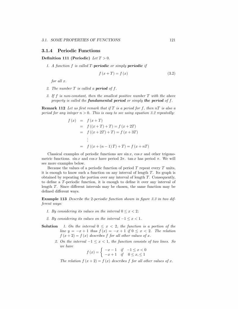
Example 113 Describe the 2-periodic function shown in figure 3.3 in two dif-ferent ways:
1. By considering its values on the interval 0 ≤ x < 2;
2. By considering its values on the interval −1 ≤ x < 1.
Solution 1. On the interval 0 ≤ x < 2, the function is a portion of theline y = −x + 1 thus f (x) = −x + 1 if 0 ≤ x < 2. The relationf (x+ 2) = f (x) describes f for all other values of x.
2. On the interval −1 ≤ x < 1, the function consists of two lines. Sowe have
f (x) =
{−x− 1 if −1 ≤ x < 0−x+ 1 if 0 ≤ x,≤ 1
The relation f (x+ 2) = f (x) describes f for all other values of x.
122 CHAPTER 3. FOURIER SERIES
Figure 3.3: A Function of Period 2
Although we have different formulas, they describe the same function. Ofcourse, in practice, we use common sense to select the most appropriate formula.Next, we look at an important theorem concerning integration of periodic
functions over one period.
Theorem 114 (Integration Over One Period) Suppose that f is T -periodic.Then for any real number a, we have∫ T
0
f (x) dx =
∫ a+T
a
f (x) dx (3.3)
Proof. Define F (a) =∫ a+T
af (x) dx. By the fundamental theorem of calculus,
F ′ (a) = f (a+ T )− f (a) = 0 since f is T -periodic. Hence, F (a) is a constantfor all a. In particular, F (0) = F (a) which implies the theorem.
We illustrate this theorem with an example.
Example 115 Let f be the 2-periodic function shown in figure 3.3. Computethe integrals below:
1.∫ 1
−1[f (x)]
2dx
2.∫ N−N [f (x)]
2dx where N is any positive integer.
Solution 116 We answer each part separately.
1. We described this function earlier and noticed that its simplest expressionwas not over the interval [−1, 1] but over the interval [0, 2]. We should
3.1. SOME PROPERTIES OF FUNCTIONS 123
also note that if f is 2-periodic, so is [f (x)]2 (why?). Using theorem 114,
we have ∫ 1
−1
[f (x)]2dx =
∫ 2
0
[f (x)]2dx
=
∫ 2
0
(−x+ 1)2dx
=−1
3(−x+ 1)
3
∣∣∣∣20
=2
3
2. We break∫ N−N [f (x)]
2dx into the sum of N integrals over intervals of
length 2.∫ N
−N[f (x)]
2dx =
∫ −N+2
−N[f (x)]
2dx+
∫ −N+4
−N+2
[f (x)]2dx+...+
∫ N
N−2
[f (x)]2dx
By theorem 114, each integral is 23 . Thus∫ N
−N[f (x)]
2dx =
2N
3
The following result about combining periodic functions is important.
Theorem 117 When combining periodic functions, the following is true:
1. If f1, f2, ..., fn are T -periodic, then a1f1 + a2f2 + ... + anfn is also T -periodic.
2. If f and g are two T -periodic functions so is f (x) g (x).
3. If f and g are two T -periodic functions so is f(x)g(x) where g (x) 6= 0.
4. If f has period T and a > 0 then f(xa
)has period aT and f (ax) has
period Ta .
5. If f has period T and g is any function (not necessarily periodic) then thecomposition g ◦ f has period T .Proof. See problems.
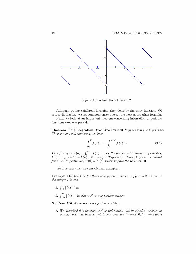
We finish this section by looking at another example of a periodic function,which does not involve trigonometric functions but rather the greatest integerfunction, also known as the floor function, denoted bxc. bxc represents thegreatest integer not larger than x. For example, b5.2c = 5, b5c = 5, b−5.2c =−6, b−5c = −5. Its graph is shown in figure 3.4.
124 CHAPTER 3. FOURIER SERIES
Figure 3.4: Graph of bxc
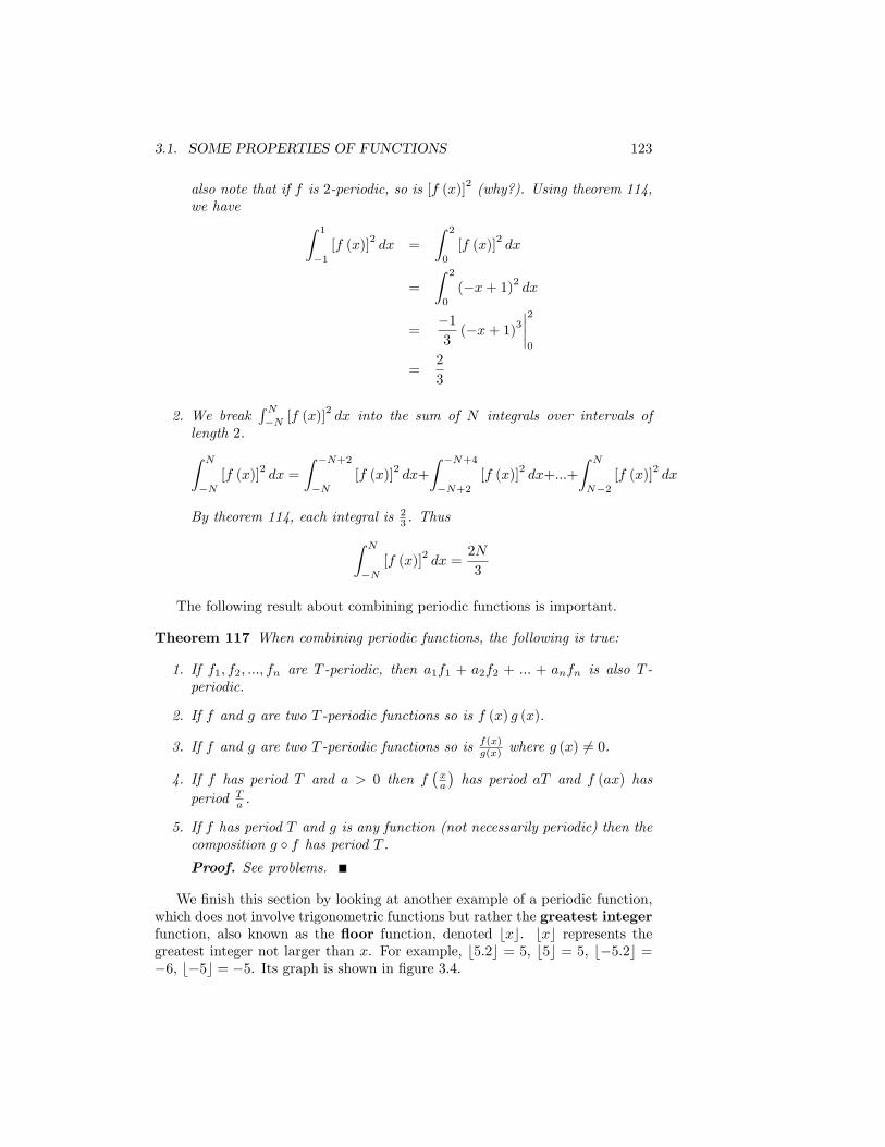
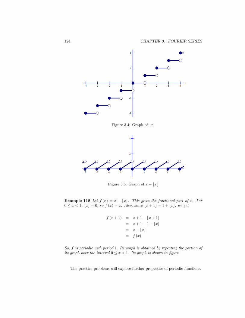
Figure 3.5: Graph of x− bxc
Example 118 Let f (x) = x − bxc. This gives the fractional part of x. For0 ≤ x < 1, bxc = 0, so f (x) = x. Also, since bx+ 1c = 1 + bxc, we get
f (x+ 1) = x+ 1− bx+ 1c= x+ 1− 1− bxc= x− bxc= f (x)
So, f is periodic with period 1. Its graph is obtained by repeating the portion ofits graph over the interval 0 ≤ x < 1. Its graph is shown in figure
The practice problems will explore further properties of periodic functions.
3.1. SOME PROPERTIES OF FUNCTIONS 125
3.1.5 Orthogonal Family of Functions
The functions in the 2L-periodic trigonometric system
1, cosπx
L, cos
2πx
L, cos
3πx
L, ..., sin
πx
L, sin
2πx
L, sin
3πx
L, ...
are among the most important periodic functions. The reader will verify thatthey are indeed 2L-periodic in the homework. They share another importantproperty.
Theorem 119 The family of functions{
1, cosnπ
Lx, sin
nπ
Lx : n ∈ N
}forms an
orthogonal family on the interval [−L,L] in other words, if m and n are twononnegative integers, then remembering that 〈f (x) , g (x)〉 =
∫ L−L f (x) g (x) dx
we have: ⟨1, cos
nπ
Lx⟩
= 0 for n = 1, 2, ... (3.4)⟨1, sin
nπ
Lx⟩
= 0 for n = 1, 2, ...⟨sin
nπ
Lx, cos
mπ
Lx⟩
= 0 ∀m,n⟨sin
nπ
Lx, sin
mπ
Lx⟩
= 0 if m 6= n⟨cos
nπ
Lx, cos
mπ
Lx⟩
= 0 if m 6= n
Proof. The proof has been done in the previous chapter over several section.We remind the reader of the important trigonometric identities which are usedin evaluating these integrals.
sinα cosβ =1
2[sin (α+ β) + sin (α− β)]
cosα sinβ =1
2[sin (α+ β)− sin (α− β)]
sinα sinβ =1
2[cos (α+ β)− cos (α− β)]
cosα cosβ =1
2[cos (α+ β) + cos (α− β)]
Remark 120 We also have the useful identities∫ L
−Lcos2 mπ
Lxdx =
∫ L
−Lsin2 mπ
Lxdx = L for all m 6= 0 (3.5)
3.1.6 Problems
1. Prove theorem 109.
126 CHAPTER 3. FOURIER SERIES
2. Prove theorem 110.
3. Sums of periodic functions. Show that if f1, f2, ..., fn are T -periodic,then a1f1 + a2f2 + ...+ anfn is also T -periodic.
4. Sums of periodic functions. Let f (x) = cosx+ cosπx.
(a) Show that the equation f (x) = 2 has a unique solution.
(b) Conclude from part a that f is not periodic. Does this contradict theprevious problem?
5. Finish proving theorem 119.
6. Operations on periodic functions.
(a) Show that if f and g are two T -periodic functions so is f (x) g (x).
(b) Show that if f and g are two T -periodic functions so is f(x)g(x) where
g (x) 6= 0.
(c) Show that if f has period T and a > 0 then f(xa
)has period aT and
f (ax) has period Ta .
(d) Show that if f has period T and g is any function (not necessarilyperiodic) then the composition g ◦ f has period T .
7. Using the previous problem, find the period of the functions below.
(a) sin 2x
(b) cos 12x+ 3 sin 2x
(c) 12+sin x
(d) ecos x
8. Show that the functions 1, cosπx
L, cos
2πx
L, cos
3πx
L, ..., sin
πx
L, sin
2πx
L, sin
3πx
L, ...
are 2L-periodic.
9. Antiderivative of periodic functions. Suppose that f is 2π-periodicand let a be a fixed real number. Define
F (x) =
∫ x
a
f (t) dt for all x
Show that F is 2π-periodic if and only if∫ 2π
0f (t) dt = 0. (hint: use
theorem 114)
3.2. FOURIER SERIES OF A FUNCTION 127
3.2 Fourier Series of a Function
3.2.1 Goal
We first review how to derive the Fourier series of a function. We then statesome important results about Fourier series.As noted earlier, Fourier Series are special expansions of functions of the
form
f (x) = A0 +
∞∑n=1
(An cos
nπx
L+Bn sin
nπx
L
)Finding the Fourier series for a given function f (x) (if it exists) amounts tofinding the coeffi cients An for n = 0, 1, 2, ... and Bn for n = 1, 2, 3, ....
3.2.2 Euler’s Formulas for the Coeffi cients
In the previous chapter, we already learned how to find the coeffi cients An andBn. We remind the reader of the formulas and look at some examples.
Definition 121 The Fourier series of a function f (x) on the interval [−L,L]where L > 0 is given by
f (x) = A0 +
∞∑n=1
(An cos
nπx
L+Bn sin
nπx
L
)(3.6)
The coeffi cients which appear in the Fourier series were known to Eulerbefore Fourier, hence they bear his name. They are given by the followingformulas.
Theorem 122 The coeffi cients in equation 3.6 are given by
A0 =1
2L
∫ L
−Lf (x) dx (3.7)
An =1
L
∫ L
−Lf (x) cos
nπx
Ldx for n = 1, 2, ... (3.8)
Bn =1
L
∫ L
−Lf (x) sin
nπx
Ldx for n = 1, 2, ... (3.9)
Definition 123 For a positive integer N , we denote the N th partial sum of theFourier series of f by SN (x). So, we have
SN (x) = A0 +
N∑n=1
(An cos
nπx
L+Bn sin
nπx
L
)We now illustrate what we did with some examples.
128 CHAPTER 3. FOURIER SERIES
3.2.3 Examples of Fourier Series
Example 124 Find the Fourier series of f (x) = sinx on [−π, π].Using the formulas above along with equation 3.6, we find that
A0 =1
2π
∫ π
−πsinxdx = 0
An =1
π
∫ π
−πsinx cosnxdx = 0 for all n
Bn =1
π
∫ π
−πsinx sinnxdx = 0 except when n = 1
When n = 1,we have A1 = 1. Thus, a Fourier series of sinx is sinx. Of course,this was to be expected.
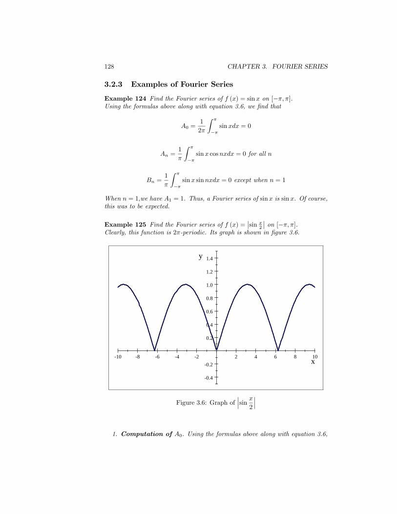
Example 125 Find the Fourier series of f (x) =∣∣sin x
2
∣∣ on [−π, π].Clearly, this function is 2π-periodic. Its graph is shown in figure 3.6.
10 8 6 4 2 2 4 6 8 10
0.4
0.2
0.2
0.4
0.6
0.8
1.0
1.2
1.4
x
y
Figure 3.6: Graph of∣∣∣sin x
2
∣∣∣
1. Computation of A0. Using the formulas above along with equation 3.6,
3.2. FOURIER SERIES OF A FUNCTION 129
we find that
A0 =1
2π
∫ π
−π
∣∣∣sin x2
∣∣∣ dx=
1
π
∫ π
0
sinx
2dx since
∣∣∣sin x2
∣∣∣ is even and sinx
2≥ 0 on [0, π]
=2
π
2. Computation of An.
An =1
π
∫ π
−π
∣∣∣sin x2
∣∣∣ cosnxdx
=2
π
∫ π
0
sinx
2cosnxdx
=1
π
∫ π
0
[sin
2n+ 1
2x− sin
2n− 1
2x
]dx if n ≥ 1
=1
π
[−2
2n+ 1cos
2n+ 1
2x+
2
2n− 1cos
2n− 1
2x
]∣∣∣∣π0
=1
π
[2
2n+ 1− 2
2n− 1
]=
−4
π (4n2 − 1)
3. Computation of Bn.
Bn =1
π
∫ π
−π
∣∣∣sin x2
∣∣∣ sinnxdx= 0 since
∫ π
−π
∣∣∣sin x2
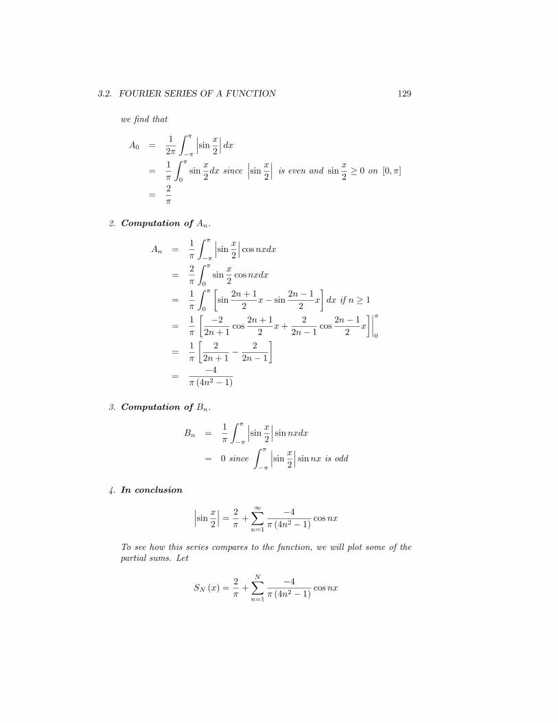
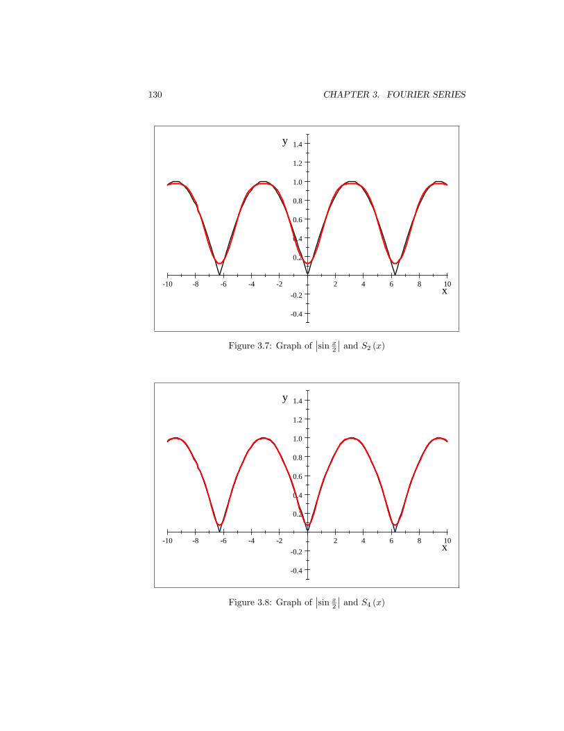
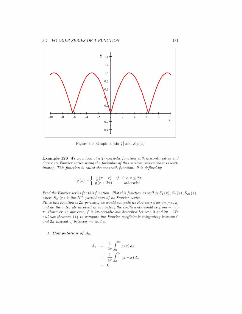
∣∣∣ sinnx is odd4. In conclusion
∣∣∣sin x2
∣∣∣ =2
π+
∞∑n=1
−4
π (4n2 − 1)cosnx
To see how this series compares to the function, we will plot some of thepartial sums. Let
SN (x) =2
π+
N∑n=1
−4
π (4n2 − 1)cosnx
130 CHAPTER 3. FOURIER SERIES
10 8 6 4 2 2 4 6 8 10
0.4
0.2
0.2
0.4
0.6
0.8
1.0
1.2
1.4
x
y
Figure 3.7: Graph of∣∣sin x
2
∣∣ and S2 (x)
10 8 6 4 2 2 4 6 8 10
0.4
0.2
0.2
0.4
0.6
0.8
1.0
1.2
1.4
x
y
Figure 3.8: Graph of∣∣sin x
2
∣∣ and S4 (x)
3.2. FOURIER SERIES OF A FUNCTION 131
10 8 6 4 2 2 4 6 8 10
0.4
0.2
0.2
0.4
0.6
0.8
1.0
1.2
1.4
x
y
Figure 3.9: Graph of∣∣sin x
2
∣∣ and S10 (x)
Example 126 We now look at a 2π-periodic function with discontinuities andderive its Fourier series using the formulas of this section (assuming it is legit-imate). This function is called the sawtooth function. It is defined by
g (x) =
{12 (π − x) if 0 < x ≤ 2πg (x+ 2π) otherwise
Find the Fourier series for this function. Plot this function as well as S1 (x) , S7 (x) , S20 (x)where SN (x) is the N th partial sum of its Fourier series.SInce this function is 2π-periodic, we would compute its Fourier series on [−π, π]and all the integrals involved in computing the coeffi cients would be from −π toπ. However, in our case, f is 2π-periodic but described between 0 and 2π . Wewill use theorem 114 to compute the Fourier coeffi cients integrating between 0and 2π instead of between −π and π.
1. Computation of A0.
A0 =1
2π
∫ 2π
0
g (x) dx
=1
4π
∫ 2π
0
(π − x) dx
= 0
132 CHAPTER 3. FOURIER SERIES
2. Computation of An.
An =1
π
∫ 2π
0
g (x) cosnxdx for n = 1, 2, ...
=1
2π
∫ 2π
0
(π − x) cosnxdx
=1
2π
[π
∫ 2π
0
cosnxdx−∫ 2π
0
x cosnxdx
]The first integral is 0. The second can be evaluated by parts.∫ 2π
0
x cosnxdx =x
nsinnx
∣∣∣2π0− 1
n
∫ 2π
0
sinnxdx
=1
n2cosnx
∣∣∣∣2π0
= 0
soAn = 0
3. Computation of Bn.
Bn =1
π
∫ 2π
0
g (x) sinnxdx for n = 1, 2, ...
=1
2π
∫ 2π
0
(π − x) sinnxdx
=1
2π
[π
∫ 2π
0
sinnxdx−∫ 2π
0
x sinnxdx
]The first integral is 0. The second can be done by parts.∫ 2π
0
x sinnxdx =−xn
cosnx
∣∣∣∣2π0
+1
n
∫ 2π
0
cosnxdx
=−2π
n+
1
n2sinnx
∣∣∣∣2π0
=−2π
n
Therefore
Bn =1
2π
[0− −2π
n
]=
1
n
3.2. FOURIER SERIES OF A FUNCTION 133
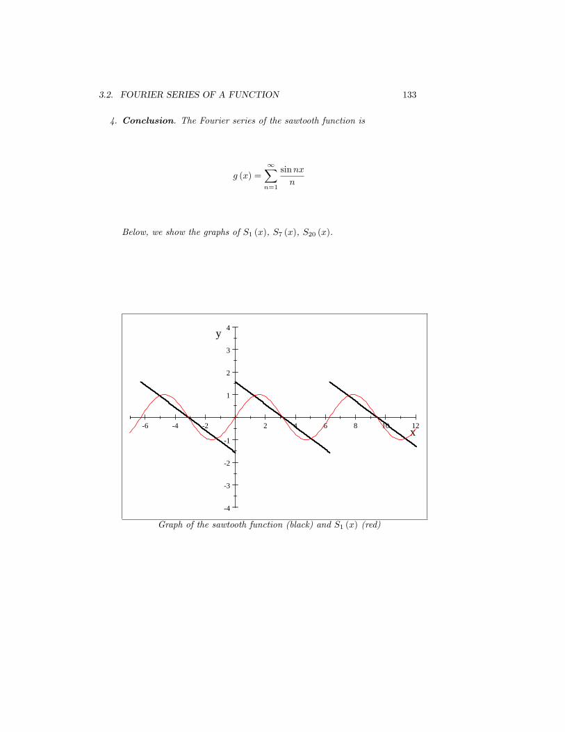
4. Conclusion. The Fourier series of the sawtooth function is
g (x) =
∞∑n=1
sinnx
n
Below, we show the graphs of S1 (x), S7 (x), S20 (x).
6 4 2 2 4 6 8 10 12
4
3
2
1
1
2
3
4
x
y
Graph of the sawtooth function (black) and S1 (x) (red)
134 CHAPTER 3. FOURIER SERIES
6 4 2 2 4 6 8 10 12
4
3
2
1
1
2
3
4
x
y
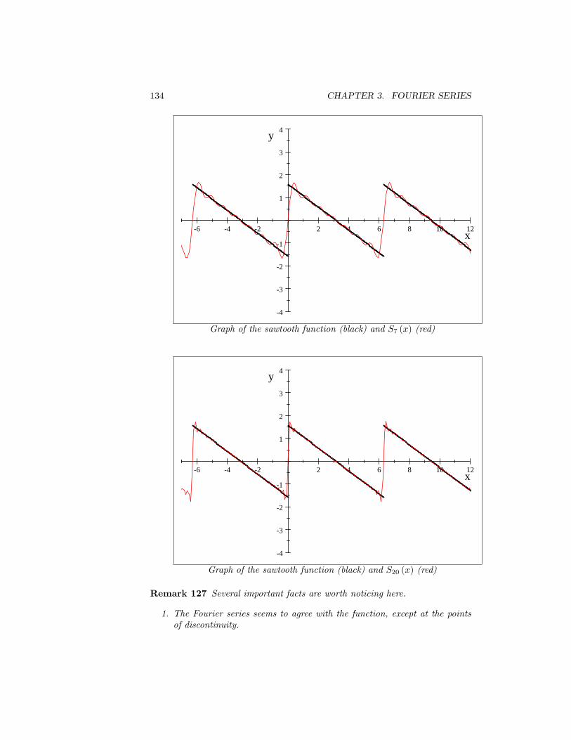
Graph of the sawtooth function (black) and S7 (x) (red)
6 4 2 2 4 6 8 10 12
4
3
2
1
1
2
3
4
x
y
Graph of the sawtooth function (black) and S20 (x) (red)
Remark 127 Several important facts are worth noticing here.
1. The Fourier series seems to agree with the function, except at the pointsof discontinuity.
3.2. FOURIER SERIES OF A FUNCTION 135
2. At the points of discontinuity, the series converges to 0, which is the av-erage value of the function from the left and from the right.
3. Near the points of discontinuity, the Fourier series overshoots its limitingvalues. This is a well known phenomenon, known as Gibbs phenom-enon. To see a simulation of this phenomenon, visit the ??
3.2.4 Piecewise Continuous and Piecewise Smooth Func-tions
After defining some useful concepts, we give a suffi cient condition for a functionto have a Fourier series representation.
Notation 128 We will denote f (c−) = limx→c−
f (x) and f (c+) = limx→c+
f (x)
Remembering that a function f is continuous at c if and only if limx→c
f (x) =
f (c), we see that a function f is continuous at c if and only if
f (c−) = f (c+) = f (c)
Definition 129 (Piecewise Continuous) A function f is said to be piece-wise continuous on the interval [a, b] if the following are satisfied:
1. f (a+) and f (b−) exist.
2. f is defined and continuous on (a, b) except possibly at a finite number ofpoints in (a, b) where the left and right limit at these points exist. Suchpoints are called jump discontinuities.
Definition 130 (Piecewise Smooth) A function f , defined on [a, b] is saidto be piecewise smooth on [a, b] if both f and f ′ are piecewise continuous on[a, b].
Example 131 The sawtooth function is piecewise smooth.
Example 132 A simple example of a function which is not piecewise smooth isx13 for −1 ≤ x ≤ 1. Its derivative does not exist at 0, neither do the one sidedlimits of its derivative at 0.
Example 133 The function f (x) =1
xis not piecewise continuous on [−1, 1]
since it is not continuous at 0 and limx→0−
f (x) does not exist.
Definition 134 The average of f at c is defined to be
f (c−) + f (c+)
2
136 CHAPTER 3. FOURIER SERIES
Clearly, if f is continuous at c, then its average at c is f (c).We are now ready to state a fundamental result in the theory of Fourier
series.
Theorem 135 Suppose that f is a piecewise smooth function on [−L,L]. Then,for all x in [−L,L], we have
f (x−) + f (x+)
2= A0 +
∞∑n=1
(An cos
nπx
L+Bn sin
nπx
L
)(3.10)
that is the Fourier series converges tof (x−) + f (x+)
2, where the coeffi cients
are given by equations 3.7, 3.8, and 3.9. In particular, if f is piecewise smoothand continuous at x, then
f (x) = A0 +
∞∑n=1
(An cos
nπx
L+Bn sin
nπx
L
)(3.11)
that is the Fourier series converges to f (x).
Thus, at points where f is continuous, the Fourier series converges to thefunction. At points of discontinuity, the series converges to the average of thefunction at these points. This was the case in the example with the sawtoothfunction.
Remark 136 In the case f is 2L-periodic, we have an even stronger result.Convergence of the Fourier series is for every x, not just for every x in [−L,L].
We do one more example.
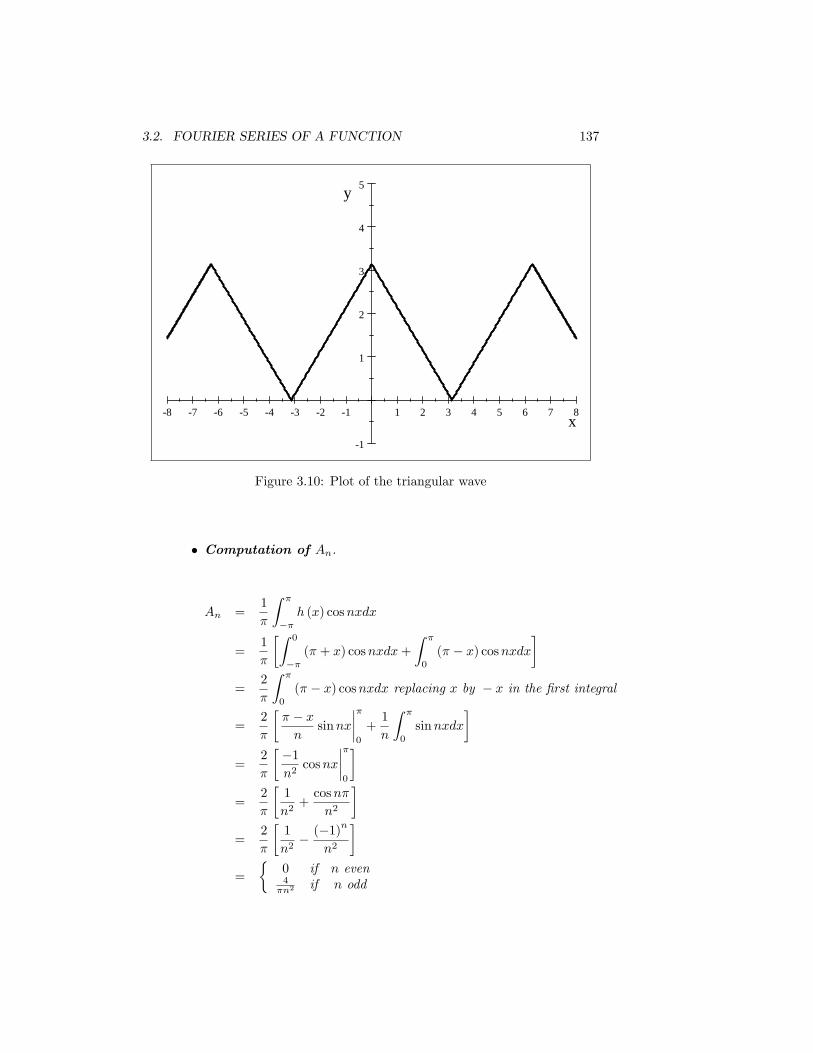
Example 137 (Triangular Wave) The 2π-periodic triangular wave is givenon the interval [−π, π] by
h (x) =
{π + x if −π ≤ x ≤ 0π − x if 0 ≤ x ≤ π
1. Find its Fourier series.
2. Plot h (x) as well as some partial sums of its Fourier series.
3. Show how this series could be used to approximate π(actually π2
).
Solution 138 1. We begin by plotting h (x)We see the function is piecewisesmooth and continuous for all x.
• Computation of A0.
A0 =1
2π
∫ π
−πh (x) dx
=1
2ππ2
=π
2
3.2. FOURIER SERIES OF A FUNCTION 137
8 7 6 5 4 3 2 1 1 2 3 4 5 6 7 8
1
1
2
3
4
5
x
y
Figure 3.10: Plot of the triangular wave
• Computation of An.
An =1
π
∫ π
−πh (x) cosnxdx
=1
π
[∫ 0
−π(π + x) cosnxdx+
∫ π
0
(π − x) cosnxdx
]=
2
π
∫ π
0
(π − x) cosnxdx replacing x by − x in the first integral
=2
π
[π − xn
sinnx
∣∣∣∣π0
+1
n
∫ π
0
sinnxdx
]=
2
π
[−1
n2cosnx
∣∣∣∣π0
]=
2
π
[1
n2+
cosnπ
n2
]=
2
π
[1
n2− (−1)
n
n2
]=
{0 if n even4πn2 if n odd
138 CHAPTER 3. FOURIER SERIES
• Computation of Bn.
Bn =1
π
∫ π
−πh (x) sinnxdx
= 0 since the integrand is odd (why?)
• Conclusion.
h (x) =π
2+
4
π
∞∑n=0
cos (2n+ 1)x
(2n+ 1)2
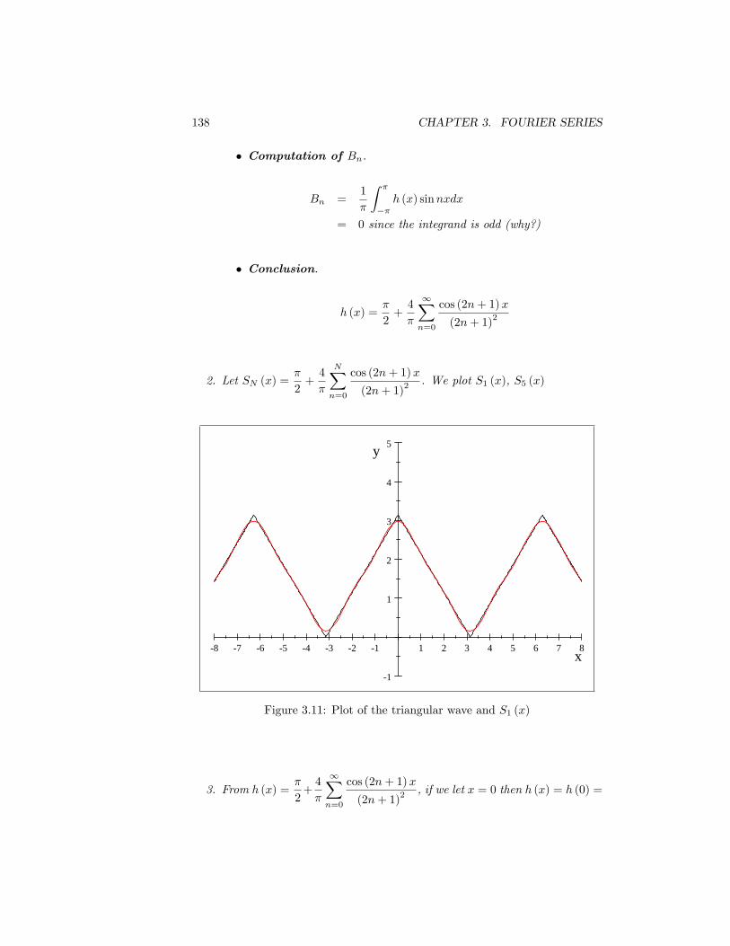
2. Let SN (x) =π
2+
4
π
N∑n=0
cos (2n+ 1)x
(2n+ 1)2 . We plot S1 (x), S5 (x)
8 7 6 5 4 3 2 1 1 2 3 4 5 6 7 8
1
1
2
3
4
5
x
y
Figure 3.11: Plot of the triangular wave and S1 (x)
3. From h (x) =π
2+
4
π
∞∑n=0
cos (2n+ 1)x
(2n+ 1)2 , if we let x = 0 then h (x) = h (0) =
3.2. FOURIER SERIES OF A FUNCTION 139
8 7 6 5 4 3 2 1 1 2 3 4 5 6 7 8
1
1
2
3
4
5
x
y
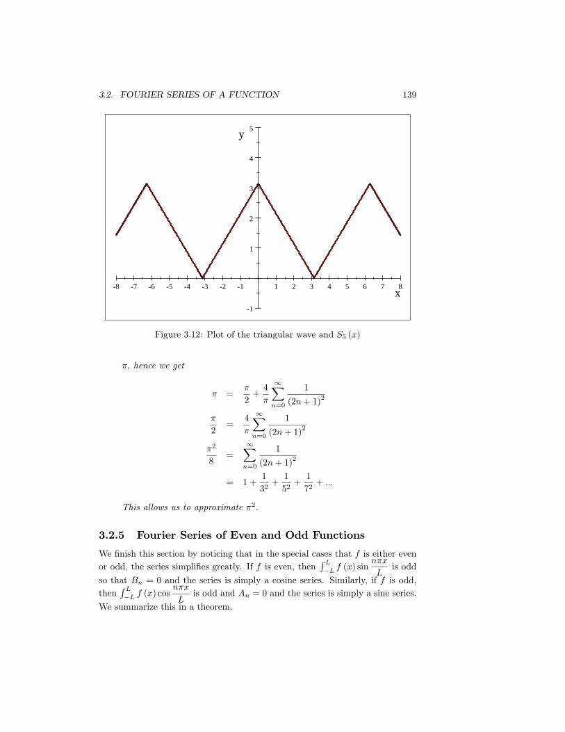
Figure 3.12: Plot of the triangular wave and S5 (x)
π, hence we get
π =π
2+
4
π
∞∑n=0
1
(2n+ 1)2
π
2=
4
π
∞∑n=0
1
(2n+ 1)2
π2
8=
∞∑n=0
1
(2n+ 1)2
= 1 +1
32+
1
52+
1
72+ ...
This allows us to approximate π2.
3.2.5 Fourier Series of Even and Odd Functions
We finish this section by noticing that in the special cases that f is either evenor odd, the series simplifies greatly. If f is even, then
∫ L−L f (x) sin
nπx
Lis odd
so that Bn = 0 and the series is simply a cosine series. Similarly, if f is odd,then
∫ L−L f (x) cos
nπx
Lis odd and An = 0 and the series is simply a sine series.
We summarize this in a theorem.
140 CHAPTER 3. FOURIER SERIES
Theorem 139 Suppose that on [−L,L] f has the Fourier series representation
f (x) = A0 +
∞∑n=1
[An cos
nπx
L+Bn sin
nπx
L
]Then:
1. If f is even then Bn = 0 for all n and in this case
f (x) = A0 +
∞∑n=1
An cosnπx
L
2. If f is odd then An = 0 for all n and in this case
f (x) =
∞∑n=1
Bn sinnπx
L
3.2.6 Periodic extensions
The most we were able to establish above is that given an arbitrary piecewisesmooth function f and an interval [−L,L], the Fourier series of f converges toeither f (if f is continuous) or the average of f on [−L,L]. We now define anew function to which the Fourier series of f will converge for all reals.
Definition 140 (Periodic Extension) Given a function f and an interval[−L,L] on which f is defined, by the periodic extension of f of period2L, we mean the new function F we obtain by taking the graph of f on theinterval [−L.L] and repeating it for the other intervals of length 2L in otherwords F (x) = f (x) if −L ≤ x ≤ L and F (x+ T ) = F (x) for all x whereT = 2L.
We illustrate this with some examples.
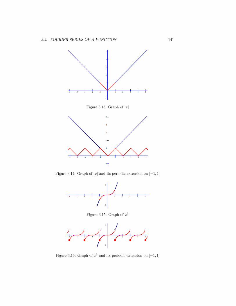
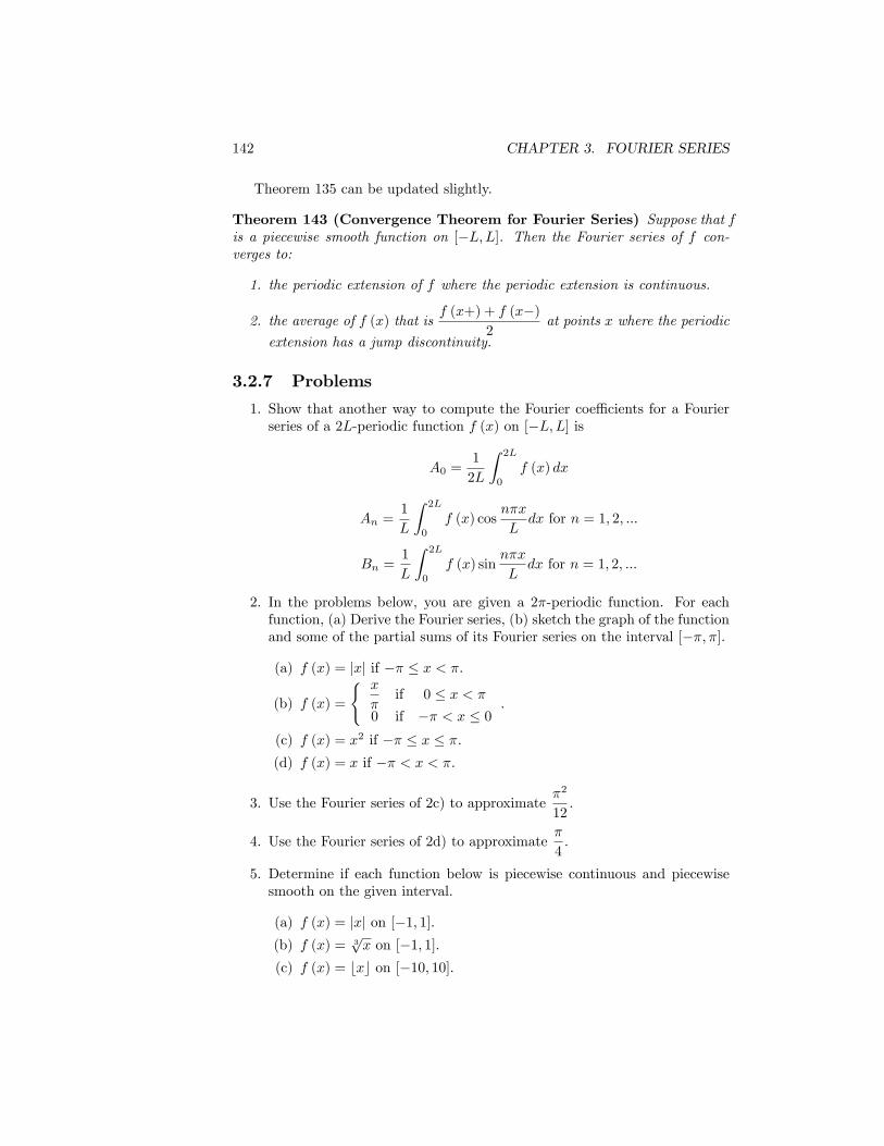
Example 141 Figure 3.13 shows the graph of y = |x|. In red is the portion ofthis graph for x ∈ [−1, 1]. We want to obtain the periodic extension of |x| on theinterval [−1, 1]. For this, we just copy the red part of the graph over and over,to the right and to the left. The periodic extension of |x| on [−1, 1] is shown infigure 3.14 in red.
In this example, the periodic extension of |x| which is continuous resulted ina continuous function. I does not have to be this way. The next example showsus a continuous function whose periodic extension is not continuous.
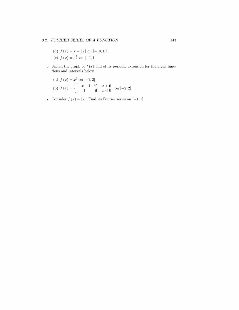
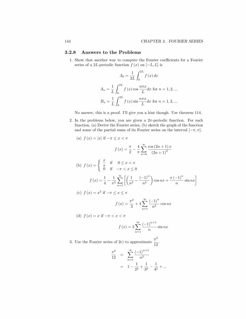
Example 142 Figure 3.15 shows the graph of y = x3. In red is the portion ofthis graph for x ∈ [−1, 1]. We want to obtain the periodic extension of x3 on theinterval [−1, 1]. For this, we just copy the red part of the graph over and over,to the right and to the left. The periodic extension of x3 on [−1, 1] is shown infigure 3.16 in red.
3.2. FOURIER SERIES OF A FUNCTION 141
Figure 3.13: Graph of |x|
Figure 3.14: Graph of |x| and its periodic extension on [−1, 1]
Figure 3.15: Graph of x3
Figure 3.16: Graph of x3 and its periodic extension on [−1, 1]
142 CHAPTER 3. FOURIER SERIES
Theorem 135 can be updated slightly.
Theorem 143 (Convergence Theorem for Fourier Series) Suppose that fis a piecewise smooth function on [−L,L]. Then the Fourier series of f con-verges to:
1. the periodic extension of f where the periodic extension is continuous.
2. the average of f (x) that isf (x+) + f (x−)
2at points x where the periodic
extension has a jump discontinuity.
3.2.7 Problems
1. Show that another way to compute the Fourier coeffi cients for a Fourierseries of a 2L-periodic function f (x) on [−L,L] is
A0 =1
2L
∫ 2L
0
f (x) dx
An =1
L
∫ 2L
0
f (x) cosnπx
Ldx for n = 1, 2, ...
Bn =1
L
∫ 2L
0
f (x) sinnπx
Ldx for n = 1, 2, ...
2. In the problems below, you are given a 2π-periodic function. For eachfunction, (a) Derive the Fourier series, (b) sketch the graph of the functionand some of the partial sums of its Fourier series on the interval [−π, π].
(a) f (x) = |x| if −π ≤ x < π.
(b) f (x) =
{ x
πif 0 ≤ x < π
0 if −π < x ≤ 0.
(c) f (x) = x2 if −π ≤ x ≤ π.(d) f (x) = x if −π < x < π.
3. Use the Fourier series of 2c) to approximateπ2
12.
4. Use the Fourier series of 2d) to approximateπ
4.
5. Determine if each function below is piecewise continuous and piecewisesmooth on the given interval.
(a) f (x) = |x| on [−1, 1].
(b) f (x) = 3√x on [−1, 1].
(c) f (x) = bxc on [−10, 10].
3.2. FOURIER SERIES OF A FUNCTION 143
(d) f (x) = x− bxc on [−10, 10].
(e) f (x) = e1x on [−1, 1].
6. Sketch the graph of f (x) and of its periodic extension for the given func-tions and intervals below.
(a) f (x) = x2 on [−1, 2]
(b) f (x) =
{−x+ 1 if x > 0
1 if x < 0on [−2, 2]
7. Consider f (x) = |x|. Find its Fourier series on [−1, 1].
144 CHAPTER 3. FOURIER SERIES
3.2.8 Answers to the Problems
1. Show that another way to compute the Fourier coeffi cients for a Fourierseries of a 2L-periodic function f (x) on [−L,L] is
A0 =1
2L
∫ 2L
0
f (x) dx
An =1
L
∫ 2L
0
f (x) cosnπx
Ldx for n = 1, 2, ...
Bn =1
L
∫ 2L
0
f (x) sinnπx
Ldx for n = 1, 2, ...
No answer, this is a proof. I’ll give you a hint though. Use theorem 114.
2. In the problems below, you are given a 2π-periodic function. For eachfunction, (a) Derive the Fourier series, (b) sketch the graph of the functionand some of the partial sums of its Fourier series on the interval [−π, π].
(a) f (x) = |x| if −π ≤ x < π
f (x) =π
2− 4
π
∞∑n=0
cos (2n+ 1)x
(2n+ 1)2
(b) f (x) =
{ x
πif 0 ≤ x < π
0 if −π < x ≤ 0
f (x) =1
4− 1
π2
∞∑n=1
[(1
n2− (−1)
n
n2
)cosnx+
π (−1)n
nsinnx
](c) f (x) = x2 if −π ≤ x ≤ π
f (x) =π2
3+ 4
∞∑n=1
(−1)n
n2cosnx
(d) f (x) = x if −π < x < π
f (x) = 2
∞∑n=1
(−1)n+1
nsinnx
3. Use the Fourier series of 2c) to approximateπ2
12.
π2
12=
∞∑n=1
(−1)n+1
n2
= 1− 1
22+
1
32− 1
42+ ...
3.2. FOURIER SERIES OF A FUNCTION 145
4. Use the Fourier series of 2d) to approximateπ
4.
π
4=
∞∑n=0
(−1)n
2n+ 1
= 1− 1
3+
1
5− 1
7+ ...
5. Determine if each function below is piecewise continuous and piecewisesmooth on the given interval.
(a) f (x) = |x| on [−1, 1].yes, yes.
(b) f (x) = 3√x on [−1, 1].
yes, no.
(c) f (x) = bxc on [−10, 10].yes, yes.
(d) f (x) = x− bxc on [−10, 10].yes, yes.
(e) f (x) = e1x on [−1, 1].
no, no.
6. Sketch the graph of f (x) and of its periodic extension for the given func-tions and intervals below.
(a) f (x) = x2 on [−1, 2]
(b) f (x) =
{−x+ 1 if x > 0
1 if x < 0on [−2, 2]
7. Consider f (x) = |x|. Find its Fourier series on [−1, 1].
|x| = 1
2+
10∑n=1
2 (−1)n − 2
(nπ)2 cosnπx
146 CHAPTER 3. FOURIER SERIES
3.3 Integration and Differentiation of Fourier Se-ries
3.3.1 Goal
When doing manipulations with infinite sums, we must remember that manyproperties which hold for finite sums do not always hold for infinite sums. Inthis section, we will see that the derivative of a sum (infinite) is not always thesums of the derivatives. In other words, we cannot always differentiate a Fourierseries term by term. In this section, we discuss continuity, differentiation andintegration of Fourier series.
3.3.2 Linearity of Fourier Series
Theorem 144 (Linearity of Fourier Series) Suppose that f1 and f2 are piece-wise smooth on [−L.L] and c1 and c2 are two constants. Then, the Fourier seriesof c1f1 (x) + c2f2 (x) is c1 times the Fourier series of f1 (x) plus c2 times theFourier series of f2 (x).
The theorem means that if for example we know the Fourier series of x andx2 then the Fourier series of x + x2 is the sum of the Fourier series of x andx2. We don’t have to go through the lengthy process of computing Euler’scoeffi cients.
3.3.3 Continuity of Fourier Series
From the convergence theorem on Fourier series (theorem 143), we know thatwhere f is continuous, its Fourier series converges to f and is therefore continu-ous. The only points at which we need to worry about are the points where wehave jump discontinuities. This can happen at points where the function itselfhas jump discontinuities. It can also happen at the endpoints of the intervalunder study. If f (−L) 6= f (L) then the periodic extension of f will have ajump discontinuity there. We have the following theorem.
Theorem 145 (Continuity of Fourier Series) Suppose that f is piecewisesmooth on the interval [−L,L]. The Fourier series of f is continuous and con-verges to f on [−L,L] if and only if f is continuous and f (−L) = f (L).
We are now ready to discuss differentiation and integration of Fourier series.
3.3.4 Differentiation of Fourier Series
Let us start with an example.
Example 146 Consider the Fourier series for f (x) = x on [−L,L]. ThisFourier series is (see homework)
x =
∞∑n=1
(−1)n+1
2L
nπsin
nπx
L(3.12)
3.3. INTEGRATION AND DIFFERENTIATION OF FOURIER SERIES147
If we differentiate the left side of equation 3.12, we get (x)′
= 1. The Fourierseries for 1 on [−L,L] is (see homework)
1 = 1
However, if we differentiate the right of equation 3.12, we get 2
∞∑n=1
(−1)n+1
cosnπx
L,
which is not the Fourier series for 1 on [−L,L] since that series is 1 (see home-work) .
So, the above example shows us we cannot always differentiate term by term.We now give without proof the conditions under which we can differentiate termby term.
Theorem 147 If f ′ is a piecewise smooth function and if f is also continuous,then the Fourier series of f can be differentiated term by term provided thatf (−L) = f (L).
We can see why the example above failed since if f (x) = x then f (−L) 6=f (L).
Remark 148 One advantage of being able to differentiate term by term is to beable to derive new Fourier series from existing ones. This bypasses the lengthyprocess of computing Euler’s coeffi cients. The example below illustrates this.
Example 149 Find a Fourier series for f (x) = −2x on [−1, 1] using the the-orem above and remembering from the homework of the previous chapter that aFourier series for 1− x2 on [−1, 1] is
1− x2 =2
3+
∞∑n=1
(−1)n+1
4
(nπ)2 cosnπx
1 − x2 satisfies the conditions of the theorem, hence we can differentiate itsFourier series term by term. So, we have
d(1− x2
)dx
=
d
(2
3
)dx
+
∞∑n=1
d
((−1)
n+14
(nπ)2 cosnπx
)dx
or
−2x =
∞∑n=1
−nπ (−1)n+1
4
(nπ)2 sinnπx
=
∞∑n=1
(−1)n
4
nπsinnπx
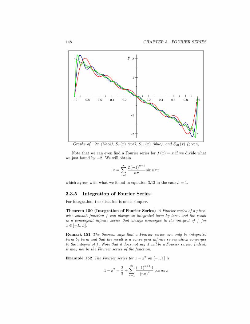
Figure 149 shows the graph of −2x along with the graph of SN (x) =
N∑n=1
(−1)n
4
nπsinnπx
for N = 5 (in red), N = 10 (in blue) and N = 20 (in green).
148 CHAPTER 3. FOURIER SERIES
1.0 0.8 0.6 0.4 0.2 0.2 0.4 0.6 0.8 1.0
2
1
1
2
x
y
Graphs of −2x (black), S5 (x) (red), S10 (x) (blue), and S20 (x) (green)
Note that we can even find a Fourier series for f (x) = x if we divide whatwe just found by −2. We will obtain
x =
∞∑n=1
2 (−1)n+1
nπsinnπx
which agrees with what we found in equation 3.12 in the case L = 1.
3.3.5 Integration of Fourier Series
For integration, the situation is much simpler.
Theorem 150 (Integration of Fourier Series) A Fourier series of a piece-wise smooth function f can always be integrated term by term and the resultis a convergent infinite series that always converges to the integral of f forx ∈ [−L,L].
Remark 151 The theorem says that a Fourier series can only be integratedterm by term and that the result is a convergent infinite series which convergesto the integral of f . Note that it does not say it will be a Fourier series. Indeed,it may not be the Fourier series of the function.
Example 152 The Fourier series for 1− x2 on [−1, 1] is
1− x2 =2
3+
∞∑n=1
(−1)n+1
4
(nπ)2 cosnπx
3.3. INTEGRATION AND DIFFERENTIATION OF FOURIER SERIES149
The theorem tells us we can integrate this series term by term. Hence∫ x
−1
(1− s2
)ds =
∫ x
−1
[2
3+
∞∑n=1
(−1)n+1
4
(nπ)2 cosnπs
]ds
=
∫ x
−1
2
3ds+
∞∑n=1
(−1)n+1
4
(nπ)2
∫ x
−1
cosnπsds
=2
3(x+ 1) +
∞∑n=1
(−1)n+1
4
(nπ)2
(1
nπsinnπs
∣∣∣∣x−1
)
=2
3(x+ 1) +
∞∑n=1
(−1)n+1
4
(nπ)2
1
nπsinnπx
=2
3(x+ 1) +
∞∑n=1
(−1)n+1
4
(nπ)3 sinnπx
The result is not a Fourier series because of the term2
3(x+ 1).
3.3.6 Problems
1. Show that the Fourier series for f (x) = x on [−L,L] is∞∑n=1
(−1)n+1
2L
nπsin
nπx
L.
2. Show that the Fourier series for f (x) = 1 on [−L,L] is 1.
3. Consider the function f (x) = x2.
(a) Find a Fourier series for f (x) in the interval [−1, 1] by using thetheorem on linearity of Fourier series and the known Fourier seriesfor 1 and 1− x2.
(b) Find a Fourier series for g (x) = x by differentiating the series youfound in part a. First, justify that you can do the differentiation.
4. Consider the function f (x) = x and its power series which we derived inproblem 1.
(a) Integrate its power series by integrating from −L to x.(b) Is the series we obtained in part a a Fourier series?
5. The general formula for the Fourier series of a piecewise smooth functionf on [−L,L] is
f (x) = A0 +
∞∑n=1
(An cos
nπx
L+Bn sin
nπx
L
)(a) Integrate this power series from −L to x.(b) From what you obtain in part a, when will
∫ x−L f (s) ds be a Fourier
series?
150 CHAPTER 3. FOURIER SERIES
3.3.7 Answers to the Problems
1. Show that the Fourier series for f (x) = x on [−L,L] is∞∑n=1
(−1)n+1
2L
nπsin
nπx
L.
No answer, this is a proof.
2. Show that the Fourier series for f (x) = 1 on [−L,L] is 1.No answer, this is a proof.
3. Consider the function f (x) = x2.
(a) Find a Fourier series for f (x) in the interval [−1, 1] by using thetheorem on linearity of Fourier series and the known Fourier seriesfor 1 and 1− x2.
x2 =1
3+
∞∑n=1
(−1)n
4
(nπ)2 cosnπx
(b) Find a Fourier series for g (x) = x by differentiating the series youfound in part a. First, justify that you can do the differentiation.
x =
∞∑n=1
(−1)n+1
2
nπsinnπx
4. Consider the function f (x) = x and its power series which we derived inproblem 1.
(a) Integrate its power series by integrating from −L to x.∫ x
−Lf (s) ds =
∞∑n=1
(−1)n
2L2
(nπ)2
[cos
nπx
L− (−1)
n]
5. The general formula for the Fourier series of a piecewise smooth functionf on [−L,L] is
f (x) = A0 +
∞∑n=1
(An cos
nπx
L+Bn sin
nπx
L
)(a) Integrate this power series from −L to x.∫ x
−Lf (s) ds = A0 (x+ L)+
∞∑n=1
L
nπ
(An sin
nπx
L−Bn
(cos
nπx
L− (−1)
n))
(b) From what you obtain in part a, when will∫ x−L f (s) ds be a Fourier
series?hint: what is the general form of a Fourier series?
3.4. SOME APPLICATIONS 151
3.4 Some Applications
In the examples, we saw how we could use Fourier series to approximate π. Oneof the main uses of Fourier series is in solving some of the differential equationsfrom mathematical physics such as the wave equation or the heat equation.Fourier developed his theory by working on the heat equation. Fourier seriesalso have applications in music synthesis and image processing. All these willbe presented in another talk. We will mention the relationship between sound(music) and Fourier series.
When we represent a signal f (t) by its Fourier series f (t) = A0+
∞∑n=1
[An cos
nπt
L+Bn sin
nπt
L
],
we are finding the contribution of each frequencynπ
Lto the signal. The value
of the corresponding coeffi cients give us that contribution. The nth term of
the partial sum of the Fourier series, An cosnπt
L+Bn sin
nπt
L, is called the nth
harmonic of f . Its amplitude is given by√An +Bn. Conversely, we can
create a signal by using the Fourier series A0 +
∞∑n=1
[An cos
nπt
L+Bn sin
nπt
L
]for a given value of L and playing with the value of the coeffi cients.
Audio signals describe air pressure variations captured by our ears and per-ceived as sounds. We will focus here on periodic audio signals also known astones. Such signals can be represented by Fourier series.A pure tone can be written as x (t) = a cos (ωt+ φ) where a > 0 is the
amplitude , ω > 0 is the frequency in radians/seconds and φ is the phase angle.An alternative way to represent the frequency is in Hertz. The frequency f inHertz is given by f =
ω
2π.
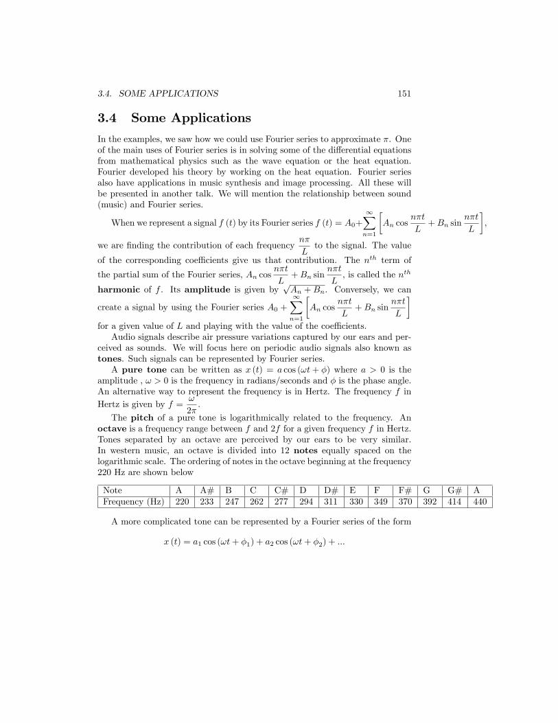
The pitch of a pure tone is logarithmically related to the frequency. Anoctave is a frequency range between f and 2f for a given frequency f in Hertz.Tones separated by an octave are perceived by our ears to be very similar.In western music, an octave is divided into 12 notes equally spaced on thelogarithmic scale. The ordering of notes in the octave beginning at the frequency220 Hz are shown below
Note A A# B C C# D D# E F F# G G# AFrequency (Hz) 220 233 247 262 277 294 311 330 349 370 392 414 440
A more complicated tone can be represented by a Fourier series of the form
x (t) = a1 cos (ωt+ φ1) + a2 cos (ωt+ φ2) + ...