Embed Size (px)
Citation preview

Fourier Series
Philippe B. Laval
Kennesaw State University
March 24, 2008
Abstract
These notes introduce Fourier series and discuss some applications.
1 Introduction
Joseph Fourier (1768-1830) who gave his name to Fourier series, was not the firstto use Fourier series neither did he answer all the questions about them. Theseseries had already been studied by Euler, d’Alembert, Bernoulli and others be-fore him. Fourier also thought wrongly that any function could be representedby Fourier series. However, these series bear his name because he studied themextensively. The first concise study of these series appeared in Fourier’s publica-tions in 1807, 1811 and 1822 in his Théorie analytique de la chaleur. He appliedthe technique of Fourier series to solve the heat equation. He had the insightto see the power of this new method. His work set the path for techniques thatcontinue to be developed even today.
Fourier Series, like Taylor series, are special types of expansion of functions.With Taylor series, we are interested in expanding a function in terms of thespecial set of functions 1, x, x2, x3, ... or more generally in terms of 1, (x− a),
(x− a)2, (x− a)3, .... You will remember from calculus that if a function f hasa power series representation at a then
f (x) =∞∑
n=0
f (n) (a)
n!(x− a)n (1)
With Fourier series, we are interested in expanding a function f in terms of thespecial set of functions 1, cosx, cos 2x, cos 3x, ..., sinx, sin 2x, sin 3x, ... Thus,a Fourier series expansion of a function is an expression of the form
f (x) = a0 +∞∑
n=1
(an cosnx+ bn sinnx)
After reviewing periodic functions, we will focus on learning how to representa function by its Fourier series. We will only partially answer the questionregarding which functions have a Fourier series representation. We will finishthese notes by discussing some applications.
1

2 Even, Odd and Periodic Functions
In this section, we review some results about even, odd and periodic functions.These results will be needed for the remaining sections.
Definition 1 (Even and Odd) Let f be a function defined on an interval I(finite or infinite) centered at x = 0.
1. f is said to be even if f (−x) = f (x) for every x in I.
2. f is said to be odd if f (−x) = −f (x) for every x in I.
The graph of an even function is symmetric with respect to the y-axis. Thegraph of an odd function is symmetric with respect to the origin. For example,5, x2, xn where n is even, cosx are even functions while x, x3, xn where n isodd, sinx are odd.
You will recall from calculus the following important theorem about inte-grating even and odd functions over an interval of the form [−a, a] where a > 0.
Theorem 2 Let f be a function which domain includes [−a, a] where a > 0.
1. If f is even, then∫ a
−af (x) dx = 2
∫ a
0f (x) dx
2. If f is odd, then∫ a
−af (x) dx = 0
There are several useful algebraic properties of even and odd functions asshown in the theorem below.
Theorem 3 When adding or multiplying even and odd functions, the followingis true:
• even + even = even
• even × even = even
• odd + odd = odd
• odd × odd = even
• even × odd = odd
Definition 4 (Periodic) Let T > 0.
1. A function f is called T -periodic or simply periodic if
f (x+ T ) = f (x) (2)
for all x.
2. The number T is called a period of f .
2
3. If f is non-constant, then the smallest positive number T with the aboveproperty is called the fundamental period or simply the period of f .
Let us first remark that if T is a period for f , then nT is also a period forany integer n > 0. This is easy to see using equation 2 repeatedly:
f (x) = f (x+ T )
= f ((x+ T ) + T ) = f (x+ 2T )
= f ((x+ 2T ) + T ) = f (x+ 3T )
...
= f ((x+ (n− 1)T ) + T ) = f (x+ nT )
Classical examples of periodic functions are sinx, cosx and other trigono-metric functions. sinx and cosx have period 2π. tanx has period π. We willsee more examples below.
Because the values of a periodic function of period T repeat every T units,it is enough to know such a function on any interval of length T . Its graph isobtained by repeating the portion over any interval of length T . Consequently,to define a T -periodic function, it is enough to define it over any interval oflength T . Since different intervals may be chosen, the same function may bedefined different ways.
Example 5 Describe the 2-periodic function shown in figure 1 in two differentways:
1. By considering its values on the interval 0 ≤ x < 2;
2. By considering its values on the interval −1 ≤ x < 1.
Solution 1. On the interval 0 ≤ x < 2, the function is a portion of theline y = −x + 1 thus f (x) = −x + 1 if 0 ≤ x < 2. The relationf (x+ 2) = f (x) describes f for all other values of x.
2. On the interval −1 ≤ x < 1, the function consists of two lines. Sowe have
f (x) =
{−x− 1 if −1 ≤ x < 0−x+ 1 if 0 ≤ x,≤ 1
The relation f (x+ 2) = f (x) describes f for all other values of x.
Although we have different formulas, they describe the same function. Ofcourse, in practice, we use common sense to select the most appropriate formula.
Next, we look at an important theorem concerning integration of periodicfunctions over one period.
Theorem 6 (Integration Over One Period) Suppose that f is T -periodic.Then for any real number a, we have∫ T
0
f (x) dx =
∫ a+T
a
f (x) dx (3)
3

Figure 1: A function of period 2
Proof. Define F (a) =∫ a+T
af (x) dx. By the fundamental theorem of calculus,
F ′ (a) = f (a+ T )− f (a) = 0 since f is T -periodic. Hence, F (a) is a constantfor all a. In particular, F (0) = F (a) which implies the theorem.
We illustrate this theorem with an example.
Example 7 Let f be the 2-periodic function shown in figure 1. Compute theintegrals below:
1.∫ 1
−1[f (x)]2 dx
2.∫ N
−N[f (x)]2 dx where N is any positive integer.
Solution 8 1. We described this function earlier and noticed that its sim-plest expression was not over the interval [−1, 1] but over the interval [0, 2].
We should also note that if f is 2-periodic, so is [f (x)]2 (why?). Usingtheorem 6, we have∫ 1
−1
[f (x)]2 dx =
∫ 2
0
[f (x)]2 dx
=
∫ 2
0
(−x+ 1)2 dx
=−1
3(−x+ 1)3
∣∣∣∣2
0
=2
3
4

2. We break∫ N
−N[f (x)]2 dx into the sum of N integrals over intervals of
length 2.
∫ N
−N
[f (x)]2 dx =
∫−N+2
−N
[f (x)]2 dx+
∫−N+4
−N+2
[f (x)]2 dx+...+
∫ N
N−2
[f (x)]2 dx
By theorem 6, each integral is 23 . Thus
∫ N
−N
[f (x)]2 dx =2N
3
The following result about combining periodic functions is important.
Theorem 9 When combining periodic functions, the following is true:
1. If f1, f2, ..., fn are T -periodic, then a1f1 + a2f2 + ... + anfn is also T -periodic.
2. If f and g are two T -periodic functions so is f (x) g (x).
3. If f and g are two T -periodic functions so is f(x)g(x) where g (x) �= 0.
4. If f has period T and a > 0 then f(xa
)has period aT and f (ax) has
period Ta.
5. If f has period T and g is any function (not necessarily periodic) then thecomposition g ◦ f has period T .
Proof. See problems.
The functions in the 2π-periodic trigonometric system
1, cosx, cos 2x, ..., cosmx, ..., sinx, sin 2x, ..., sinnx, ...
are among the most important periodic functions. The reader will verify thatthey are indeed 2π-periodic. They share another important property.
Definition 10 (Orthogonal Functions) Two functions f and g are said tobe orthogonal over the interval [a, b] if
∫ b
a
f (x) g (x) dx = 0 (4)
The notion of orthogonality is very important in many areas of mathematics.
5

Theorem 11 The functions in the trigonometric system 1, cosx, cos 2x, ..., cosmx, ..., sinx, sin 2x, ..., sinnx, ...are orthogonal over the interval [−π, π] in other words, if m and n are two non-negative integers, then∫ π
−π
cosmx cosnxdx = 0 if m �= n (5)∫ π
−π
cosmx sinnxdx = 0 ∀m,n∫ π
−π
sinmx sinnxdx = 0 if m �= n
Proof. There are different ways to prove this theorem. One way involves usingthe identities
sinα cosβ =1
2[sin (α+ β) + sin (α− β)]
cosα sinβ =1
2[sin (α+ β)− sin (α− β)]
sinα sinβ =1
2[cos (α+ β)− cos (α− β)]
cosα cosβ =1
2[cos (α+ β) + cos (α− β)]
We illustrate the technique by proving∫ π
−πcosmx cosnxdx = 0 if m �= n. We
see that cosmx cosnx = 12 [cos (m+ n)x+ cos (m− n)x]. Therefore∫ π
−π
cosmx cosnxdx =1
2
∫ π
−π
[cos (m+ n)x+ cos (m− n)] dx
=1
2
[1
m+ nsin (m+ n)x+
1
m− nsin (m− n)x
]∣∣∣∣π
−π
= 0
Remark 12 We also have the useful identities∫ π
−π
cos2 mxdx =
∫ π
−π
sin2 mxdx = π for all m �= 0 (6)
We finish this section by looking at another example of a periodic function,which does not involve trigonometric function but rather the greatest integerfunction, also known as the floor function, denoted �x�. �x� represents thegreatest integer not larger than x. For example, �5.2� = 5, �5� = 5, �−5.2� =−6, �−5� = −5. Its graph is shown in figure 2.
Example 13 Let f (x) = x − �x�. This gives the fractional part of x. For
6

-5 -4 -3 -2 -1 1 2 3 4 5
-5
-4
-3
-2
-1
1
2
3
4
x
y
Figure 2: Graph of �x�
0 ≤ x < 1, �x� = 0, so f (x) = x. Also, since �x+ 1� = 1 + �x�, we get
f (x+ 1) = x+ 1− �x+ 1�
= x+ 1− 1− �x�
= x− �x�
= f (x)
So, f is periodic with period 1. Its graph is obtained by repeating the portion ofits graph over the interval 0 ≤ x < 1. Its graph is shown in figure
The practice problem will explore further properties of periodic functions.
2.1 Practice Problems
1. Prove theorem 2.
2. Prove theorem 3.
3. Sums of periodic functions. Show that if f1, f2, ..., fn are T -periodic,then a1f1 + a2f2 + ...+ anfn is also T -periodic.
4. Sums of periodic functions. Let f (x) = cosx+ cosπx.
(a) Show that the equation f (x) = 2 has a unique solution.
7

-5 -4 -3 -2 -1 1 2 3 4 5
-1
1
2
3
4
5
x
y
Figure 3: Graph of x− �x�
(b) Conclude from part a that f is not periodic. Does this contradict theprevious problem?
5. Finish proving theorem 11.
6. Operations on periodic functions.
(a) Show that if f and g are two T -periodic functions so is f (x) g (x).
(b) Show that if f and g are two T -periodic functions so is f(x)g(x) where
g (x) �= 0.
(c) Show that if f has period T and a > 0 then f(xa
)has period aT and
f (ax) has period Ta.
(d) Show that if f has period T and g is any function (not necessarilyperiodic) then the composition g ◦ f has period T .
7. Using the previous problem, find the period of the functions below.
(a) sin 2x
(b) cos 12x+ 3 sin 2x
(c) 12+sin x
(d) ecos x
8

8. Antiderivative of periodic functions. Suppose that f is 2π-periodicand let a be a fixed real number. Define
F (x) =
∫ x
a
f (t) dt for all x
Show that F is 2π-periodic if and only if∫ 2π
0f (t) dt = 0. (hint: use
theorem 6)
3 Fourier Series of 2π-Periodic Functions
As noted earlier, Fourier Series are special expansions of functions of the form
f (x) = a0 +∞∑
n=1
(an cosnx+ bn sinnx) (7)
To be able to use Fourier Series, we need to know:
1. Which functions have Fourier series expansions?
2. If a function has a Fourier series expansion, how do we compute the coef-ficients a0, a1, ..., b0, b1, ...?
A general answer to the first question is beyond the scope of these notes. Inthis section, we will answer the second question. In these notes, we will giveconditions which are sufficient for functions to have a Fourier Series Expansion.
3.1 Euler Formulas for the Coefficients
The coefficients which appear in the Fourier series were known to Euler beforeFourier, hence they bear his name. We will derive them the same way Fourierdid. This technique is worth remembering.
• Computation of a0. Starting with equation 7, we integrate each sideover the interval [−π, π] and assuming term by term integration is legiti-mate, we obtain∫ π
−π
f (x) dx = a0
∫ π
−π
dx+∞∑
n=1
[an
∫ π
−π
cosnxdx+ bn
∫ π
−π
sinnxdx
]
Since∫ π
−πcosnxdx =
∫ π
−πsinnxdx = 0 for n = 1, 2, 3, ..., we have∫ π
−π
f (x) dx = a0
∫ π
−π
dx
= 2πa0
Thus
a0 =1
2π
∫ π
−π
f (x) dx
9

• Computation of an. Again, starting with equation 7, we multiply eachside by cosmx for a fixed integer m ≥ 1 and integrate each side as before.We obtain∫ π
−π
f (x) cosmxdx = a0
∫ π
−π
cosmxdx+∞∑
n=1
[an
∫ π
−π
cosnx cosmxdx+ bn
∫ π
−π
sinnx cosmxdx
]
Now, from equation 5, we have:∫ π
−πcosmxdx = 0,
∫ π
−πsinnx cosmxdx =
0 and∫ π
−πcosnx cosmxdx =
{0 if m �= n
π if m = n. So, we are left with
∫ π
−π
f (x) cosmxdx = πam
Thus
am =1
π
∫ π
−π
f (x) cosmxdx for m ≥ 1
• Computation of bn. We proceed in a similar way. Starting with equation7, we multiply each side by sinmx for a fixed integer m ≥ 1 and integrateeach side as before. We leave it to the reader to verify that
bm =1
π
∫ π
−π
f (x) sinmxdx for m ≥ 1
We summarize our findings in the following proposition.
Proposition 14 Suppose that the 2π-periodic function f has the Fourier seriesrepresentation
f (x) = a0 +∞∑
n=1
(an cosnx+ bn sinnx)
Then the coefficients a0, an, bn for n = 1, 2, ... are called the Fourier coefficientsof f and are given by the Euler’s formulas
a0 =1
2π
∫ π
−π
f (x) dx (8)
an =1
π
∫ π
−π
f (x) cosnxdx for n = 1, 2, ... (9)
bn =1
π
∫ π
−π
f (x) sinnxdx for n = 1, 2, ... (10)
Definition 15 For a positive integer N , we denote the N th partial sum of theFourier series of f by SN (x). So, we have
SN (x) = a0 +N∑
n=1
(an cosnx+ bn sinnx)
10

We now illustrate what we did with some examples.
Example 16 Find the Fourier series of f (x) = sinx.Using the formulas above along with equation 7, we find that
a0 =1
2π
∫ π
−π
sinxdx = 0
an =1
π
∫ π
−π
sinx cosnxdx = 0 for all n
bn =1
π
∫ π
−π
sinx sinnxdx = 0 except when n = 1
When n = 1,we have a1 = 1. Thus, a Fourier series of sinx is sinx. Of course,this was to be expected.
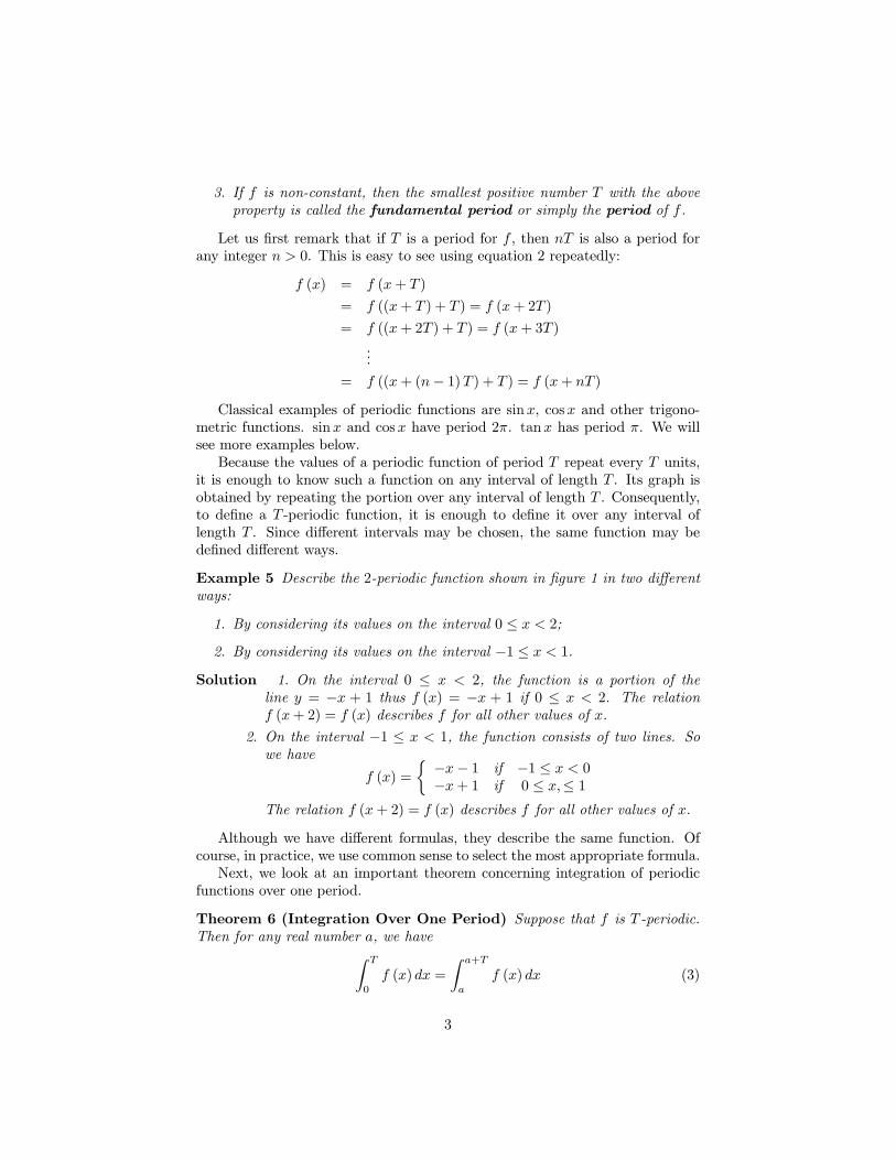
Example 17 Find the Fourier series of f (x) =∣∣sin x
2
∣∣.Clearly, this function is 2π-periodic. Its graph is shown in figure 4.
-10 -8 -6 -4 -2 2 4 6 8 10
-0.4
-0.2
0.2
0.4
0.6
0.8
1.0
1.2
1.4
x
y
Figure 4: Graph of |sinx|
1. Computation of a0. Using the formulas above along with equation 7,
11

we find that
a0 =1
2π
∫ π
−π
∣∣∣sin x
2
∣∣∣ dx=
1
π
∫ π
0
sinx
2dx since
∣∣∣sin x
2
∣∣∣ is even and sinx
2≥ 0 on [0, π]
=2
π
2. Computation of an.
an =1
π
∫ π
−π
∣∣∣sin x
2
∣∣∣ cosnxdx=
2
π
∫ π
0
sinx
2cosnxdx
=1
π
∫ π
0
[sin
2n+ 1
2x− sin
n− 1
2x
]dx if n ≥ 1
=1
π
[−2
2n+ 1cos
2n+ 1
2x+
2
2n− 1cos
2n− 1
2x
]∣∣∣∣π
0
=1
π
[2
2n+ 1−
2
2n− 1
]
=−4
π (4n2 − 1)
3. Computation of bn.
bn =1
π
∫ π
−π
|sinx| sinnxdx
= 0 since
∫ π
−π
|sinx| sinnx is odd
4. In conclusion
∣∣∣sin x
2
∣∣∣ = 2
π+
∞∑n=1
−4
π (4n2 − 1)cosnx
To see how this series compares to the function, we will plot some of thepartial sums. Let
SN (x) =2
π+
N∑n=1
−4
π (4n2 − 1)cosnx
12

-10 -8 -6 -4 -2 2 4 6 8 10
-0.4
-0.2
0.2
0.4
0.6
0.8
1.0
1.2
1.4
x
y
Figure 5: Graph of∣∣sin x
2
∣∣ and S2 (x)
-10 -8 -6 -4 -2 2 4 6 8 10
-0.4
-0.2
0.2
0.4
0.6
0.8
1.0
1.2
1.4
x
y
Figure 6: Graph of∣∣sin x
2
∣∣ and S4 (x)
13
-10 -8 -6 -4 -2 2 4 6 8 10
-0.4
-0.2
0.2
0.4
0.6
0.8
1.0
1.2
1.4
x
y
Figure 7: Graph of∣∣sin x
2
∣∣ and S10 (x)
Example 18 We now look at a 2π-periodic function with discontinuities andderive its Fourier series using the formulas of this section (assuming it is legit-imate). This function is called the sawtooth function. It is defined by
g (x) =
{12 (π − x) if 0 < x ≤ 2πg (x+ 2π) otherwise
Find the Fourier series for this function. Plot this function as well as S1 (x) , S7 (x) , S20 (x)where SN (x) is the N th partial sum of its Fourier series.Since f is described between 0 and 2π, we can use theorem 6 to compute theFourier coefficients integrating between 0 and 2π.
1. Computation of a0.
a0 =1
2π
∫ 2π
0
f (x) dx
=1
4π
∫ 2π
0
(π − x) dx
= 0
14

2. Computation of an.
an =1
π
∫ 2π
0
f (x) cosnxdx for n = 1, 2, ...
=1
2π
∫ 2π
0
(π − x) cosnxdx
=1
2π
[π
∫ 2π
0
cosnxdx−
∫ 2π
0
x cosnxdx
]
The first integral is 0. The second can be evaluated by parts.∫ 2π
0
x cosnxdx =x
nsinnx
∣∣∣2π0
−1
n
∫ 2π
0
sinnxdx
=1
n2cosnx
∣∣∣∣2π
0
= 0
soan = 0
3. Computation of bn.
bn =1
π
∫ 2π
0
f (x) sinnxdx for n = 1, 2, ...
=1
2π
∫ 2π
0
(π − x) sinnxdx
=1
2π
[π
∫ 2π
0
sinnxdx−
∫ 2π
0
x sinnxdx
]
The first integral is 0. The second can be done by parts.
∫ 2π
0
x sinnxdx =−x
ncosnx
∣∣∣∣2π
0
+1
n
∫ 2π
0
cosnxdx
=−2π
n+
1
n2sinnx
∣∣∣∣2π
0
=−2π
n
Therefore
bn =1
2π
[0−
−2π
n
]
=1
n
15

4. Conclusion. The Fourier series of the sawtooth function is
g (x) =∞∑
n=1
sinnx
n
Below, we show the graphs of S1 (x), S7 (x), S20 (x).
-6 -4 -2 2 4 6 8 10 12
-4
-3
-2
-1
1
2
3
4
x
y
Graph of the sawtooth function (black) and S1 (x) (red)
-6 -4 -2 2 4 6 8 10 12
-4
-3
-2
-1
1
2
3
4
x
y
Graph of the sawtooth function (black) and S7 (x) (red)
16

-6 -4 -2 2 4 6 8 10 12
-4
-3
-2
-1
1
2
3
4
x
y
Graph of the sawtooth function (black) and S20 (x) (red)
Remark 19 Several important facts are worth noticing here.
1. The Fourier series seems to agree with the function, except at the pointsof discontinuity.
2. At the points of discontinuity, the series converges to 0, which is the av-erage value of the function from the left and from the right.
3. Near the points of discontinuity, the Fourier series overshoots its limitingvalues. This is a well known phenomenon, known as Gibbs phenom-
enon. To see a simulation of this phenomenon, visit the ??
3.2 Piecewise Continuous and Piecewise Smooth Func-
tions
After defining some useful concepts, we give a sufficient condition for a functionto have a Fourier series representation.
Notation 20 We will denote f (c−) = limx→c−
f (x) and f (c+) = limx→c+
f (x)
Remembering that a function f is continuous at c if limx→c
f (x) = f (c), we
see that a function f is continuous at c if and only if
f (c−) = f (c+) = f (c)
17

Definition 21 (Piecewise Continuous) A function f is said to be piecewisecontinuous on the interval [a, b] if the following are satisfied:
1. f (a+) and f (b−) exist.
2. f is defined and continuous on (a, b) except at a finite number of pointsin (a, b) where the left and right limit at these points exist.
Definition 22 (Piecewise Smooth) A function f , defined on [a, b] is said tobe piecewise smooth if f and f ′ are piecewise continuous on [a, b] that is if thefollowing are satisfied:
1. f is piecewise continuous on [a, b]
2. f ′ exists on (a, b) except possibly at finitely many points in (a, b) wheretheone sided limits of f ′ at these points exists.
3. limx→a+
f ′ (x) and limx→b−
f ′ (x) exists.
The sawtooth function is piecewise smooth. A simple example of a functionwhich is not piecewise smooth is x
1
3 for −1 ≤ x ≤ 1. Its derivative does notexist at 0, neither do the one sided limits of its derivative at 0.
Definition 23 The average of f at c is defined to be
f (c−) + f (c+)
2
Clearly, if f is continuous at c, then its average at c is f (c).We are now ready to state a fundamental result in the theory of Fourier
series.
Theorem 24 Suppose that f is a 2π-periodic piecewise smooth function. Then,for all x, we have
f (x−) + f (x+)
2= a0 +
∞∑n=1
(an cosnx+ bn sinnx) (11)
where the coefficients are given by equations 8, 9, and 10. In particular, if f ispiecewise smooth and continuous at x, then
f (x) = a0 +∞∑
n=1
(an cosnx+ bn sinnx) (12)
Thus, at points where f is continuous, the Fourier series converges to thefunction. At points of discontinuity, the series converges to the average of thefunction at these points. This was the case in the example with the sawtoothfunction.
We do one more example.
18

Example 25 (Triangular Wave) The 2π-periodic triangular wave is givenon the interval [−π, π] by
h (x) =
{π + x if −π ≤ x ≤ 0π − x if 0 ≤ x ≤ π
1. Find its Fourier series.
2. Plot h (x) as well as some partial sums of its Fourier series.
3. Show how this series could be used to approximate π(actually π2
).
Solution 26 1. We begin by plotting h (x)We see the function is piecewise
-8 -7 -6 -5 -4 -3 -2 -1 1 2 3 4 5 6 7 8
-1
1
2
3
4
5
x
y
Figure 8: Plot of the triangular wave
smooth and continuous for all x.
• Computation of a0.
a0 =1
2π
∫ π
−π
f (x) dx
=1
2ππ2
=π
2
19
• Computation of an.
an =1
π
∫ π
−π
f (x) cosnxdx
=1
π
[∫ 0
−π
(π + x) cosnxdx+
∫ π
0
(π − x) cosnxdx
]
=2
π
∫ π
0
(π − x) cosnxdx replacing x by − x in the first integral
=2
π
[π − x
nsinnx
∣∣∣∣π
0
+1
n
∫ π
0
sinnxdx
]
=2
π
[−1
n2cosnx
∣∣∣∣π
0
]
=2
π
[1
n2+
cosnπ
n2
]
=2
π
[1
n2−
(−1)n
n2
]
=
{0 if n even4
πn2if n odd
• Computation of bn.
bn =1
π
∫ π
−π
f (x) sinnxdx
= 0 since the integrand is odd
• Conclusion.
h (x) =π
2+
4
π
∞∑n=0
cos (2n+ 1)x
(2n+ 1)2
2. Let SN (x) = π2 + 4
π
N∑n=0
cos(2n+1)x
(2n+1)2. We plot S1 (x), S5 (x)
3. From h (x) = π2 + 4
π
∞∑n=0
cos(2n+1)x
(2n+1)2, if we let x = 0, we get
π =π
2+
4
π
∞∑n=0
1
(2n+ 1)2
π
2=
4
π
∞∑n=0
1
(2n+ 1)2
π2
8=
∞∑n=0
1
(2n+ 1)2
= 1 +1
32+
1
52+
1
72+ ...
20

-8 -7 -6 -5 -4 -3 -2 -1 1 2 3 4 5 6 7 8
-1
1
2
3
4
5
x
y
Figure 9: Plot of the triangular wave and S1 (x)
-8 -7 -6 -5 -4 -3 -2 -1 1 2 3 4 5 6 7 8
-1
1
2
3
4
5
x
y
Figure 10: Plot of the triangular wave and S5 (x)
21
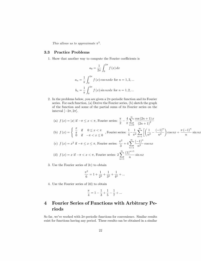
This allows us to approximate π2.
3.3 Practice Problems
1. Show that another way to compute the Fourier coefficients is
a0 =1
2π
∫ 2π
0
f (x) dx
an =1
π
∫ 2π
0
f (x) cosnxdx for n = 1, 2, ...
bn =1
π
∫ 2π
0
f (x) sinnxdx for n = 1, 2, ...
2. In the problems below, you are given a 2π-periodic function and its Fourierseries. For each function, (a) Derive the Fourier series, (b) sketch the graphof the function and some of the partial sums of its Fourier series on theinterval [−2π, 2π].
(a) f (x) = |x| if −π ≤ x < π, Fourier series:π
2−
4
π
∞∑n=0
cos (2n+ 1)x
(2n+ 1)2
(b) f (x) =
{ x
πif 0 ≤ x < π
0 if −π < x ≤ 0, Fourier series:
1
4−
1
π2
∞∑n=1
[(1
n2−
(−1)n
n2
)cosnx+
π (−1)n
nsinnx
]
(c) f (x) = x2 if −π ≤ x ≤ π, Fourier series:π2
3+ 4
∞∑n=1
(−1)n
n2cosnx
(d) f (x) = x if −π < x < π, Fourier series: 2∞∑
n=1
(1)n+1
nsinnx
3. Use the Fourier series of 2c) to obtain
π2
6= 1 +
1
22+
1
32+
1
42+ ...
4. Use the Fourier series of 2d) to obtain
π
4= 1−
1
3+
1
5−
1
7+ ...
4 Fourier Series of Functions with Arbitrary Pe-
riods
So far, we’ve worked with 2π-periodic functions for convenience. Similar resultsexist for functions having any period. These results can be obtained in a similar
22

manner. However, there is an easier way, one calculus II students are familiarwith: substitution. One way to obtain a new series representation is to performa substitution in a known series. Suppose that f is a function with period T =2p > 0 for which we want to find a Fourier series. In other words f (x+ 2p) =
f (x). If we let t =πx
pand we define
g (t) = f (x) = f
(pt
π
)
Then, g has period2pp
π
that is 2π. So, g has a Fourier series representation
g (t) = a0 +∞∑
n=1
[an cosnt+ bn sinnt]
where
a0 =1
2π
∫ π
−π
g (t) dt
an =1
π
∫ π
−π
g (t) cosntdt
bn =1
π
∫ π
−π
g (t) sin tdt
Using the substitution t =πx
p, we obtain
g
(πx
p
)= a0 +
∞∑n=1
[an cos
nπx
p+ bn sin
nπx
p
]
that is
f (x) = a0 +∞∑
n=1
[an cos
nπx
p+ bn sin
nπx
p
]
Using the same substitution, we can express the Fourier coefficients in terms of
x and f . We do it for a0. If t =πx
pthen dt =
π
pdx so
a0 =1
2π
∫ π
−π
g (t) dt
=1
2π
π
p
∫ p
−p
g
(πx
p
)dx
=1
2p
∫ p
−p
f (x) dx
So, we have the following:
23
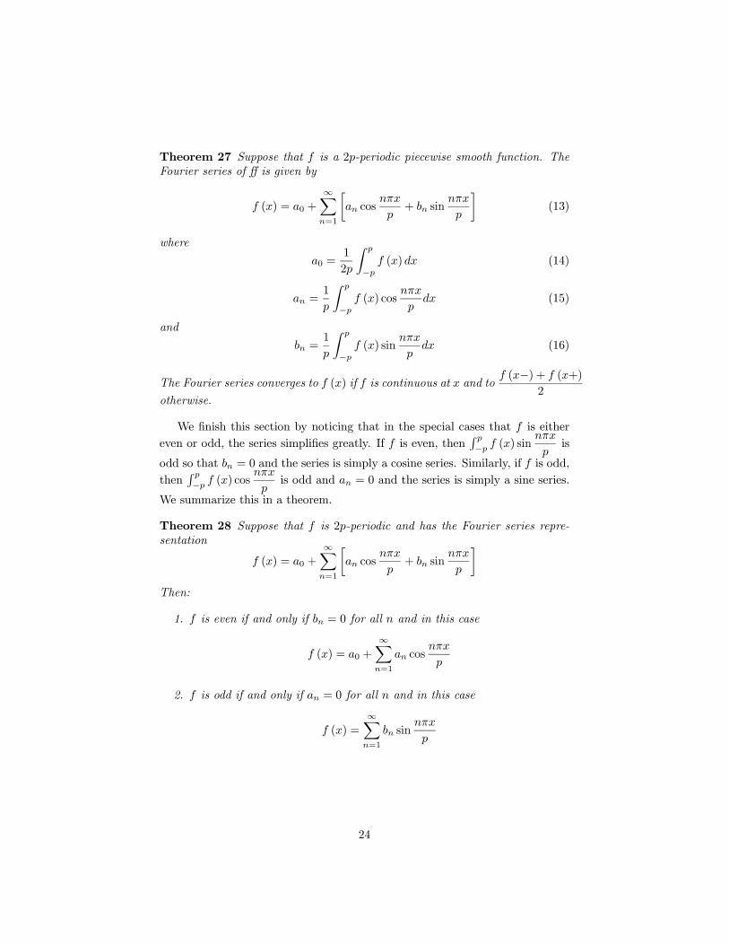
Theorem 27 Suppose that f is a 2p-periodic piecewise smooth function. TheFourier series of ff is given by
f (x) = a0 +∞∑
n=1
[an cos
nπx
p+ bn sin
nπx
p
](13)
where
a0 =1
2p
∫ p
−p
f (x) dx (14)
an =1
p
∫ p
−p
f (x) cosnπx
pdx (15)
and
bn =1
p
∫ p
−p
f (x) sinnπx
pdx (16)
The Fourier series converges to f (x) if f is continuous at x and tof (x−) + f (x+)
2otherwise.
We finish this section by noticing that in the special cases that f is either
even or odd, the series simplifies greatly. If f is even, then∫ p
−pf (x) sin
nπx
pis
odd so that bn = 0 and the series is simply a cosine series. Similarly, if f is odd,
then∫ p
−pf (x) cos
nπx
pis odd and an = 0 and the series is simply a sine series.
We summarize this in a theorem.
Theorem 28 Suppose that f is 2p-periodic and has the Fourier series repre-sentation
f (x) = a0 +∞∑
n=1
[an cos
nπx
p+ bn sin
nπx
p
]
Then:
1. f is even if and only if bn = 0 for all n and in this case
f (x) = a0 +∞∑
n=1
an cosnπx
p
2. f is odd if and only if an = 0 for all n and in this case
f (x) =∞∑
n=1
bn sinnπx
p
24

5 Some Applications
In the examples, we saw how we could use Fourier series to approximate π. Oneof the main uses of Fourier series is in solving some of the differential equationsfrom mathematical physics such as the wave equation or the heat equation.Fourier developed his theory by working on the heat equation. Fourier seriesalso have applications in music synthesis and image processing. All these willbe presented in another talk. We will mention the relationship between sound(music) and Fourier series.
When we represent a signal f (t) by its Fourier series f (t) = a0+∞∑
n=1
[an cos
nπt
p+ bn sin
nπt
p
],
we are finding the contribution of each frequencynπ
pto the signal. The value
of the corresponding coefficients give us that contribution. The nth term of the
partial sum of the Fourier series, an cosnπt
p+ bn sin
nπt
p, is called the nth har-
monic of f . Its amplitude is given by√a2n + b2n. Conversely, we can create a
signal by using the Fourier series a0 +∞∑
n=1
[an cos
nπt
p+ bn sin
nπt
p
]for a given
value of p and playing with the value of the coefficients.Audio signals describe air pressure variations captured by our ears and per-
ceived as sounds. We will focus here on periodic audio signals also known astones. Such signals can be represented by Fourier series.
A pure tone can be written as x (t) = a cos (ωt+ φ) where a > 0 is theamplitude , ω > 0 is the frequency in radians/seconds and φ is the phase angle.An alternative way to represent the frequency is in Hertz. The frequency f in
Hertz is given by f =ω
2π.
The pitch of a pure tone is logarithmically related to the frequency. Anoctave is a frequency range between f and 2f for a given frequency f in Hertz.Tones separated by an octave are perceived by our ears to be very similar.In western music, an octave is divided into 12 notes equally spaced on thelogarithmic scale. The ordering of notes in the octave beginning at the frequency220 Hz are shown below
Note A A# B C C# D D# E F F# G G# AFrequency (Hz) 220 233 247 262 277 294 311 330 349 370 392 414 440
A more complicated tone can be represented by a Fourier series of the form
x (t) = a1 cos (ωt+ φ1) + a2 cos (ωt+ φ2) + ...
References
[NA] N. H. Asmar, Partial Differential Equations and Boundary Value Prob-lems, Prentice Hall, Upper Saddle River, NJ, 2000.
25

[MG] M. D. Greenberg, Advanced Engineering Mathematics, Prentice Hall, Up-per Saddle River, NJ, 2nd ed., 1998.
[DM] D. A. McQuarrie, Mathematical Methods for Scientists and Engineers,University Science Books, Sausalito, CA, 2003.
[WS] W. Strauss, Partial Differential Equations: An Introduction, Wiley, 2008.
26