Embed Size (px)
Citation preview
Fourier Analysis
Tom Leinster
2013–14
Contents
A Preparing the ground 2A1 The algebraist’s dream . . . . . . . . . . . . . . . . . . . . . . . . 2A2 Pseudo-historical overview . . . . . . . . . . . . . . . . . . . . . . 5A3 Integration . . . . . . . . . . . . . . . . . . . . . . . . . . . . . . 8A4 What does it mean for a sequence of functions to converge? . . . 12A5 Periodic functions . . . . . . . . . . . . . . . . . . . . . . . . . . 16A6 The inner product . . . . . . . . . . . . . . . . . . . . . . . . . . 18A7 Characters and Fourier series . . . . . . . . . . . . . . . . . . . . 20A8 Trigonometric polynomials . . . . . . . . . . . . . . . . . . . . . . 22A9 Integrable functions are sort of continuous . . . . . . . . . . . . . 24
B Convergence of Fourier series in the 2- and 1-norms 28B1 Nothing is better than a Fourier partial sum . . . . . . . . . . . . 28B2 Convolution: definition and examples . . . . . . . . . . . . . . . . 31B3 Convolution: properties . . . . . . . . . . . . . . . . . . . . . . . 33B4 The mythical delta function . . . . . . . . . . . . . . . . . . . . . 36B5 Positive approximations to delta . . . . . . . . . . . . . . . . . . 38B6 Summing the unsummable . . . . . . . . . . . . . . . . . . . . . . 41B7 The Fejer kernel . . . . . . . . . . . . . . . . . . . . . . . . . . . 44B8 The main theorem . . . . . . . . . . . . . . . . . . . . . . . . . . 47
C Uniform and pointwise convergence of Fourier series 49C1 Warm-up . . . . . . . . . . . . . . . . . . . . . . . . . . . . . . . 49C2 What if the Fourier coefficients are absolutely summable? . . . . 52C3 Continuously differentiable functions . . . . . . . . . . . . . . . . 53C4 Fejer’s theorem . . . . . . . . . . . . . . . . . . . . . . . . . . . . 55C5 Differentiable functions and the Riemann localization principle . 58C6 Weyl’s equidistribution theorem . . . . . . . . . . . . . . . . . . . 61
D Duality 66D1 An abstract view of Fourier analysis . . . . . . . . . . . . . . . . 66D2 The dual of a finite abelian group . . . . . . . . . . . . . . . . . . 70D3 Fourier transforms on a finite abelian group . . . . . . . . . . . . 73D4 Fourier inversion on a finite abelian group . . . . . . . . . . . . . 77
1
Chapter A
Preparing the ground
A1 The algebraist’s dream
For the lecture of 13 January 2014
The algebraist thinks: ‘Analysis is hard. Can we reduce it to algebra?’
Idea Use power series.
1 Many functions f : R→ C can be written as a power series,
f(x) =
∞∑n=0
cnxn. (A:1)
If we can deal with the sequence (cn) rather than the function f , everythingwill be much easier (and more algebraic).
2 If we can express f in this way, then the coefficients cn must be given by
cn =f (n)(0)
n!.
(Proof: differentiate each side of (A:1) n times, then evaluate at 0.)
3 Problem:∑cnx
n might not converge. Or, it might converge, but not to f(x).
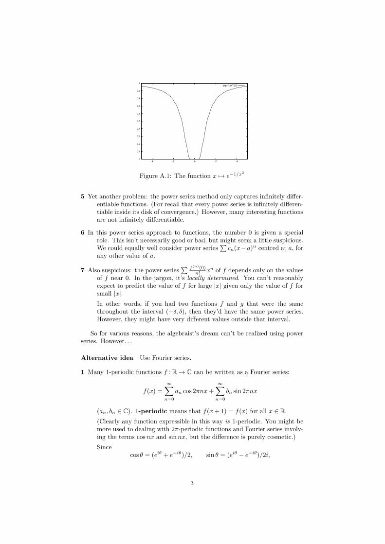
E.g. put
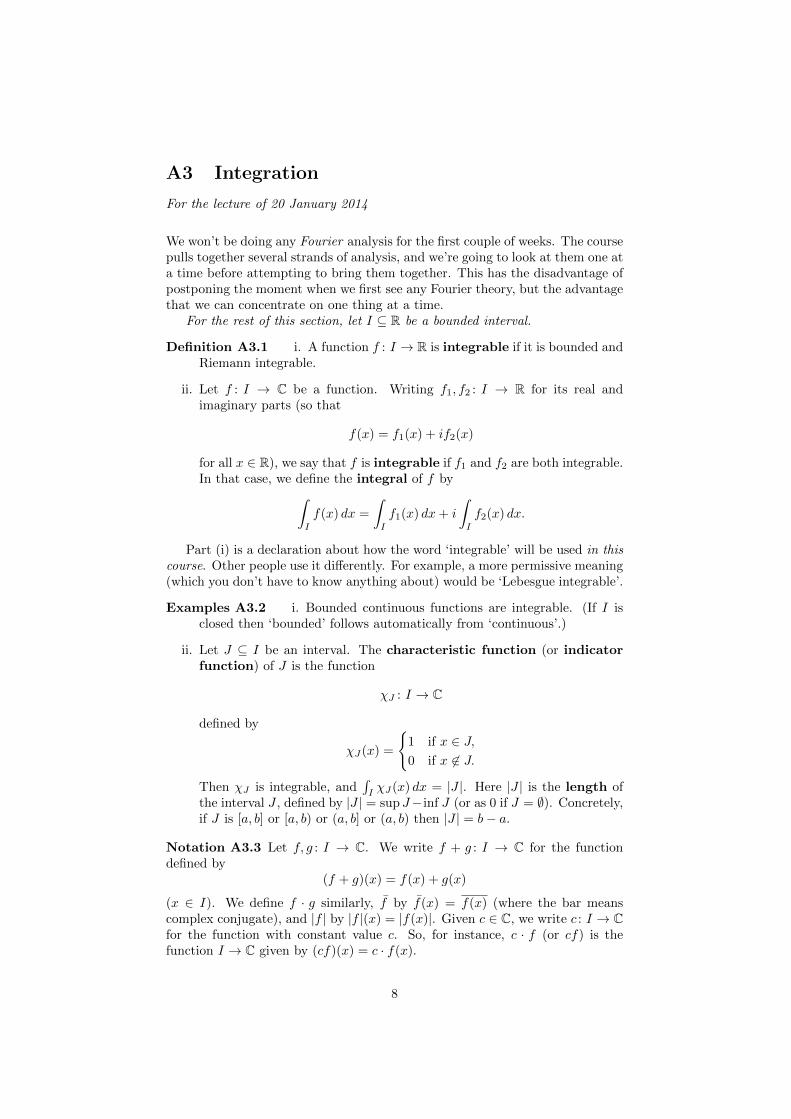
f(x) =
{e−1/x2
if x 6= 0,
0 if x = 0
(Figure A.1). It can be shown that f (n)(0)/n! = 0 for all n (which youmight guess from the flatness of the function near 0). But of course f(x) 6=∑∞n=0 0 · xn except at x = 0. This brings to light:
4 Another problem: different infinitely differentiable functions can have thesame power series. (E.g. this is the case for the f just defined and theconstant function 0.)
2
0
0.1
0.2
0.3
0.4
0.5
0.6
0.7
0.8
0.9
1
-4 -2 0 2 4
exp(-1/(x**2))
Figure A.1: The function x 7→ e−1/x2
5 Yet another problem: the power series method only captures infinitely differ-entiable functions. (For recall that every power series is infinitely differen-tiable inside its disk of convergence.) However, many interesting functionsare not infinitely differentiable.
6 In this power series approach to functions, the number 0 is given a specialrole. This isn’t necessarily good or bad, but might seem a little suspicious.We could equally well consider power series
∑cn(x−a)n centred at a, for
any other value of a.
7 Also suspicious: the power series∑ f(n)(0)
n! xn of f depends only on the valuesof f near 0. In the jargon, it’s locally determined. You can’t reasonablyexpect to predict the value of f for large |x| given only the value of f forsmall |x|.In other words, if you had two functions f and g that were the samethroughout the interval (−δ, δ), then they’d have the same power series.However, they might have very different values outside that interval.
So for various reasons, the algebraist’s dream can’t be realized using powerseries. However. . .
Alternative idea Use Fourier series.
1 Many 1-periodic functions f : R→ C can be written as a Fourier series:
f(x) =
∞∑n=0
an cos 2πnx+
∞∑n=0
bn sin 2πnx
(an, bn ∈ C). 1-periodic means that f(x+ 1) = f(x) for all x ∈ R.
(Clearly any function expressible in this way is 1-periodic. You might bemore used to dealing with 2π-periodic functions and Fourier series involv-ing the terms cosnx and sinnx, but the difference is purely cosmetic.)
Sincecos θ = (eiθ + e−iθ)/2, sin θ = (eiθ − e−iθ)/2i,
3
we can rewrite this more efficiently as
f(x) =
∞∑k=−∞
cke2πikx
for certain ck ∈ C. (Note that the sum starts at −∞.)
2 If we can express f in this way, then the coefficients ck must be given by
ck =
∫ 1
0
f(x)e−2πikx dx.
(We’ll see why later, or you can try proving it now.)
3 Problem:∑cke
2πikx might not converge. Or, it might converge, but not tof(x). (There are examples of both these phenomena.)
4 But unlike for power series, different continuous functions always have differ-ent Fourier series.
5 And unlike for power series, functions of many kinds can be captured usingFourier series. Far from having to be infinitely differentiable, even somediscontinuous functions can be captured.
6 And again unlike for power series, in the definition of ck, no point in R isgiven a special role.
7 And once more unlike for power series, the Fourier series∑cke
2πikx of f
depends on all of f (since ck =∫ 1
0f(x)e−2πikx dx, and the periodic func-
tion f is determined by its restriction to [0, 1]). In the jargon, it’s globallydetermined. So it’s not unreasonable to expect to be able to predict thevalue of f for all x given only the Fourier coefficients ck. We’ll see thatwe often can.
The algebraist’s dream can’t be fully realized. But Fourier series come closerto realizing it than power series do, at least for periodic functions on R. They’renot as obvious an idea as power series, but in many ways they work better.
We’ll spend a lot of the course exploring the extent to which functions can beunderstood in terms of their Fourier series. There are many analytic subtleties,which we’ll have to think hard about.
The development of Fourier theory has been very important historically. Ithas been the spur for a lot of important ideas in mathematics, not all obviouslyconnected to Fourier analysis. We’ll meet some along the way.
4
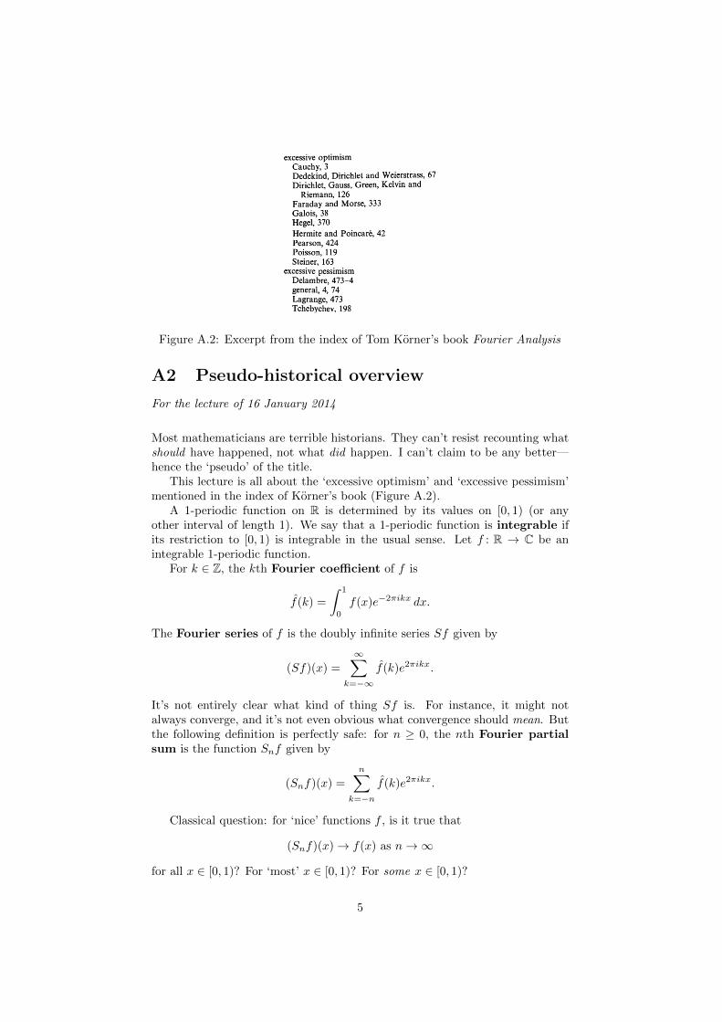
Figure A.2: Excerpt from the index of Tom Korner’s book Fourier Analysis
A2 Pseudo-historical overview
For the lecture of 16 January 2014
Most mathematicians are terrible historians. They can’t resist recounting whatshould have happened, not what did happen. I can’t claim to be any better—hence the ‘pseudo’ of the title.
This lecture is all about the ‘excessive optimism’ and ‘excessive pessimism’mentioned in the index of Korner’s book (Figure A.2).
A 1-periodic function on R is determined by its values on [0, 1) (or anyother interval of length 1). We say that a 1-periodic function is integrable ifits restriction to [0, 1) is integrable in the usual sense. Let f : R → C be anintegrable 1-periodic function.
For k ∈ Z, the kth Fourier coefficient of f is
f(k) =
∫ 1
0
f(x)e−2πikx dx.
The Fourier series of f is the doubly infinite series Sf given by
(Sf)(x) =
∞∑k=−∞
f(k)e2πikx.
It’s not entirely clear what kind of thing Sf is. For instance, it might notalways converge, and it’s not even obvious what convergence should mean. Butthe following definition is perfectly safe: for n ≥ 0, the nth Fourier partialsum is the function Snf given by
(Snf)(x) =
n∑k=−n
f(k)e2πikx.
Classical question: for ‘nice’ functions f , is it true that
(Snf)(x)→ f(x) as n→∞
for all x ∈ [0, 1)? For ‘most’ x ∈ [0, 1)? For some x ∈ [0, 1)?
5
This is the question of pointwise convergence. There are other kinds ofconvergence, as we’ll see, some of which are important in ways that pointwiseconvergence is not.
Fourier himself (1768–1830) thought that yes, it’s always true. But he wasimprecise about this (and most other things). It’s not even clear what he wouldhave taken the word ‘function’ to mean.
To start with a point that was certainly clear to Fourier himself, it can’tbe true for all x and all f . For instance, suppose it’s true for all x for someparticular f . Define g to be the same as f except at one point of [0, 1), where
it takes some different value. Then g(k) = f(k) for all k, so Sng = Snf for alln, so it can’t also be true that (Sng)(x)→ g(x) as n→∞ for all x.
(For instance, take g to be the 1-periodic function given by g(x) = 1 forx ∈ Z and g(x) = 0 for x 6∈ Z. Then for all n, the function Sng has constantvalue 0, so (Sng)(x) 6→ g(x) whenever x ∈ Z.)
Backing up Fourier’s intuition, Dirichlet proved:
Theorem A2.1 (Dirichlet, 1829) Let f : R → C be a 1-periodic, continu-ously differentiable function. Then (Snf)(x)→ f(x) as n→∞ for all x ∈ [0, 1)(or equivalently, for all x ∈ R).
Once Dirichlet had proved that, it was generally believed that ‘infinitelydifferentiable’ could be relaxed to ‘continuous’—that it was just a matter of timebefore someone figured out a proof that would work in this wider generality.
Most of the most prominent mathematicians of the day believed this. Dirich-let believed it, Cauchy, believed it, and Riemann, Weierstrass, Dedekind andPoisson all believed it. Cauchy even claimed he’d proved it. (Standards ofrigour were lower in those days.) Dirichlet promised he’d prove it, but neverdid.
But then came a bombshell.
Theorem A2.2 (du Bois-Reymond, 1876) There is a 1-periodic, contin-uous function f : R → C such that for some x ∈ [0, 1), the sequence((Snf)(x)
)∞n=0
fails to converge.
Using this example, it takes comparatively little effort to construct a 1-periodic continuous function such that ((Snf)(x))∞n=0 fails to converge at 10points, or 100, or 1000:
Theorem A2.3 Let E ⊆ [0, 1) be a finite set. Then there is a 1-periodic, con-tinuous function f : R→ C such that for all x ∈ E, the sequence
((Snf)(x)
)∞n=0
fails to converge.
Widespread pessimism ensued. The pendulum swung from the general con-sensus that Fourier series behave perfectly for all continuous functions to theopposite extreme. After du Bois-Reymond’s theorem appeared, it came to bebelieved that there was some 1-periodic continuous function f : R→ C with theproperty that for all x ∈ [0, 1), the sequence
((Snf)(x)
)∞n=0
fails to converge.This pessimism was reinforced by a further example:
Theorem A2.4 (Kolmogorov, 1926) There exists a 1-periodic, Lebesgue in-tegrable function f : R → C such that for all x ∈ [0, 1), the sequence((Snf)(x)
)∞n=0
fails to converge.
6
We won’t be doing Lebesgue integrability in this course, and I won’t assumeyou know anything about it. But as general cultural background:
Remark A2.5 Every Riemann integrable function is Lebesgue integrable. (Inparticular, a Lebesgue integrable function need not be continuous, and Kol-mogorov’s example certainly wasn’t.) Moreover, the Lebesgue integral of aRiemann integrable function is equal to its Riemann integral. However, thereare functions that are Lebesgue integrable but not Riemann integrable. So, thetheory of Lebesgue integration extends, and is more powerful than, the Riemanntheory.
This situation persisted until relatively recently. For instance, one of thebooks on my own undergraduate reading list was Apostol’s 1957 text Mathe-matical Analysis. In most respects, it is like today’s textbooks, but he states init that it’s still unknown whether for a continuous function, the Fourier serieshas to converge at even one point.
The turning point came in the 1960s.
Theorem A2.6 (Carleson, 1964) Let f : R→ C be a 1-periodic function.
• If f is continuous then (Snf)(x) → f(x) as n → ∞ for at least onex ∈ [0, 1).
• Better still, if f is Riemann integrable then (Snf)(x) → f(x) as n → ∞for at least one x ∈ [0, 1).
• Better still, if f is Riemann integrable then (Snf)(x) → f(x) as n → ∞for almost all x ∈ [0, 1). (‘Almost all’ will be defined later.)
• Even better still, if |f |2 is Lebesgue integrable (which is true if f is Rie-mann integrable) then (Snf)(x)→ f(x) as n→∞ for almost all x ∈ [0, 1).
All known proofs of Carleson’s theorem are hard, still far too hard for acourse such as this.
(I say ‘still’ because most hard proofs of important facts are simplified overtime. This was a big theorem that attracted a lot of attention, so lots of peoplehave put in lots of work to simplify the proof. They have simplified it, butit’s still well beyond our reach. This is true even for the very watered-downversion of Carleson’s theorem in the first bullet point: that for merely continuousfunctions, there is merely one point at which the Fourier series behaves well.)
Carleson’s theorem is best possible, in a sense that can be made precise(Theorem A3.18). Roughly, this means that you can’t do any better than ‘al-most all’. It almost completely answers the question of pointwise convergence ofFourier series. But there are other types of convergence too, and the behaviourof Fourier series from those points of view is interesting too, and has provokeda lot of mathematical developments—as we shall see.
7
A3 Integration
For the lecture of 20 January 2014
We won’t be doing any Fourier analysis for the first couple of weeks. The coursepulls together several strands of analysis, and we’re going to look at them one ata time before attempting to bring them together. This has the disadvantage ofpostponing the moment when we first see any Fourier theory, but the advantagethat we can concentrate on one thing at a time.
For the rest of this section, let I ⊆ R be a bounded interval.
Definition A3.1 i. A function f : I → R is integrable if it is bounded andRiemann integrable.
ii. Let f : I → C be a function. Writing f1, f2 : I → R for its real andimaginary parts (so that
f(x) = f1(x) + if2(x)
for all x ∈ R), we say that f is integrable if f1 and f2 are both integrable.In that case, we define the integral of f by∫
I
f(x) dx =
∫I
f1(x) dx+ i
∫I
f2(x) dx.
Part (i) is a declaration about how the word ‘integrable’ will be used in thiscourse. Other people use it differently. For example, a more permissive meaning(which you don’t have to know anything about) would be ‘Lebesgue integrable’.
Examples A3.2 i. Bounded continuous functions are integrable. (If I isclosed then ‘bounded’ follows automatically from ‘continuous’.)
ii. Let J ⊆ I be an interval. The characteristic function (or indicatorfunction) of J is the function
χJ : I → C
defined by
χJ(x) =
{1 if x ∈ J,0 if x 6∈ J.
Then χJ is integrable, and∫IχJ(x) dx = |J |. Here |J | is the length of
the interval J , defined by |J | = supJ− inf J (or as 0 if J = ∅). Concretely,if J is [a, b] or [a, b) or (a, b] or (a, b) then |J | = b− a.
Notation A3.3 Let f, g : I → C. We write f + g : I → C for the functiondefined by
(f + g)(x) = f(x) + g(x)
(x ∈ I). We define f · g similarly, f by f(x) = f(x) (where the bar meanscomplex conjugate), and |f | by |f |(x) = |f(x)|. Given c ∈ C, we write c : I → Cfor the function with constant value c. So, for instance, c · f (or cf) is thefunction I → C given by (cf)(x) = c · f(x).
8
Lemma A3.4 i. If f, g : I → C are integrable then so is f + g, with∫I
(f + g)(x) dx =
∫I
f(x) dx+
∫I
g(x) dx.
ii. If f : I → C is integrable and c ∈ C then cf is integrable, with∫I
(cf)(x) dx = c
∫I
f(x) dx.
iii. If f : I → C is integrable then so is f , with∫I
f(x) dx =
∫I
f(x) dx.
Proof Parts (i) and (ii) follow from the corresponding properties of real-valuedintegration, and part (iii) follows directly from the definitions. �
I’ll occasionally state ‘Facts’, without proof. Some of these facts were provedin previous courses (such as PAA). Others weren’t, and I’ll be asking you to takethose on trust.
Fact A3.5 Let f : I → C be an integrable function and φ : C→ C a continuousfunction. Then the composite φ ◦ f : I → C is integrable.
Example A3.6 If f is integrable then so is |f |p, for any real p > 0. (Takeφ(z) = |z|p.)
Lemma A3.7 If f, g : I → C are integrable then so is f · g : I → C.
Proof See Sheet 1, q.3. �
(If you’ve come across Lebesgue integration, you may be aware that boththis lemma and Example A3.6 fail for Lebesgue integration. This is one respectin which the Riemann theory makes life simpler.)
Fact A3.8 If f, g : I → R are integrable and f(x) ≤ g(x) for all x ∈ I then∫If(x) dx ≤
∫Ig(x) dx.
Note that this is for functions into R, not C; inequalities makes no sense inC.
Lemma A3.9 (Triangle inequality for integration) If f : I → C is inte-grable then |f | is integrable, with∣∣∣∣∫
I
f(x) dx
∣∣∣∣ ≤ ∫I
|f |(x) dx.
Proof That |f | is integrable is a special case of Example A3.6. Since∫If(x) dx
is a complex number, we may write∫I
f(x) dx = u
∣∣∣∣∫I
f(x) dx
∣∣∣∣9
for some u ∈ C with |u| = 1. Now∣∣∣∣∫I
f(x) dx
∣∣∣∣ = Re
∣∣∣∣∫I
f(x) dx
∣∣∣∣ = Re( 1
u
∫I
f(x) dx)
= Re
∫I
1
uf(x) dx
=
∫I
Re( 1
uf(x)
)dx (A:2)
≤∫I
∣∣∣ 1uf(x)
∣∣∣ dx (A:3)
=
∫I
|f(x)| dx =
∫I
|f |(x) dx.
Here Re(z) denotes the real part of a complex number z, equation (A:2) followsfrom the definition of complex-valued integration (Definition A3.1(ii)), the in-equality (A:3) follows from Fact A3.8 and the fact that Re(z) ≤ |z| for all z ∈ C,and the rest follow either from earlier lemmas or directly from the definitions.�
We now come to a very important concept. It was introduced by Lebesgue,and forms part of his theory of integration; and although we are not studyingthat theory, we will need this one particular concept.
Definition A3.10 A subset E of R has measure zero (or is null) if for allε > 0, there exists a sequence of intervals (Jn)∞n=1 in R such that
E ⊆∞⋃n=1
Jn and
∞∑n=1
|Jn| ≤ ε.
Examples A3.11 i. Any countable set E ⊆ R has measure zero. This isclear for E = ∅, so assume E 6= ∅. We can choose a sequence (xn)∞n=1 suchthat E = {x1, x2, . . .}. Let ε > 0. Put Jn =
(xn−2−(n+1)ε, xn+2−(n+1)ε
).
Then E ⊆⋃En and
∑|Jn| =
∑∞n=1 2−nε = ε.
ii. There also exist uncountable sets of measure zero (such as the Cantor set).
iii. If E has measure zero and F ⊆ E then F has measure zero.
iv. Let J be an interval with |J | > 0. (This condition just means that J isnot empty or of the form {a}.) Then J does not have measure zero. Thisis not as obvious as it sounds. If you do think it’s obvious, try proving it!
Definition A3.12 Let S ⊆ R. A property P of points x ∈ S holds almosteverywhere (a.e.), or for almost all x ∈ S, if there is some E ⊆ S of measurezero such that P holds for all x ∈ S \ E.
For example, if f, g : I → C then
‘f = g a.e.’
and
‘f(x) = g(x) for almost all x’
both mean: there exists a subset E ⊆ I of measure zero such that f(x) = g(x)for all x ∈ I \ E.
What’s this got to do with integration?
10
Fact A3.13 If f, g : I → C are integrable and f = g a.e. then∫If(x) dx =∫
Ig(x) dx.
Fact A3.14 If h : I → R is integrable, h(x) ≥ 0 for all x ∈ I, and∫Ih(x) dx =
0, then h = 0 a.e..
Proposition A3.15 Let f, g : I → C be integrable functions with f = g a.e..Assume that |I| > 0.
i. Let x ∈ I. If f and g are both continuous at x, then f(x) = g(x).
ii. If f and g are continuous then f = g.
Proof For (i), suppose for a contradiction that f(x) 6= g(x). By continuity, wecan find some δ > 0 such that f(t) 6= g(t) for all t ∈ (x − δ, x + δ) ∩ I. Also,since f = g a.e., we can choose E ⊆ I of measure zero such that f(t) = g(t) forall t ∈ I \E. Then (x− δ, x+ δ)∩ I ⊆ E, so (x− δ, x+ δ)∩ I has measure zeroby Example A3.11(iii). But |I| > 0, so (x− δ, x+ δ) ∩ I is an interval of length> 0, contradicting Example A3.11(iv).
Part (ii) follows immediately. �
The next result makes no mention of the concept of measure zero.
Proposition A3.16 Let h : I → R be an integrable function with h(t) ≥ 0 forall t ∈ I and
∫Ih(t) dt = 0. Assume that |I| > 0.
i. Let x ∈ I. If h is continuous at x, then h(x) = 0.
ii. If h is continuous then h = 0.
Proof We could deduce this from Fact A3.14 and Proposition A3.15. This isunnecessarily complicated, though. Sheet 1, q.4 asks you to find a direct proof.�
∗ ∗ ∗
The last two results of this lecture are non-examinable, and are included justfor background.
Fact A3.17 A function f : I → C is integrable if and only if it is bounded andcontinuous a.e. (that is, the set {x ∈ I : f is not continuous at x} has measurezero).
For example, χQ∩[0,1] : [0, 1]→ C is not integrable, since the set of disconti-nuities is [0, 1], which does not have measure zero.
At the end of the last lecture, I said that in a certain sense, Carleson’stheorem (Theorem A2.6) cannot be improved. Here is the precise statement.
Theorem A3.18 (Kahane and Katznelson, 1960s) Let E ⊆ [0, 1] be a setof measure zero. Then there is a 1-periodic, continuous function f : R→ C suchthat for all x ∈ E, the sequence
((Snf)(x)
)∞n=0
fails to converge.
11
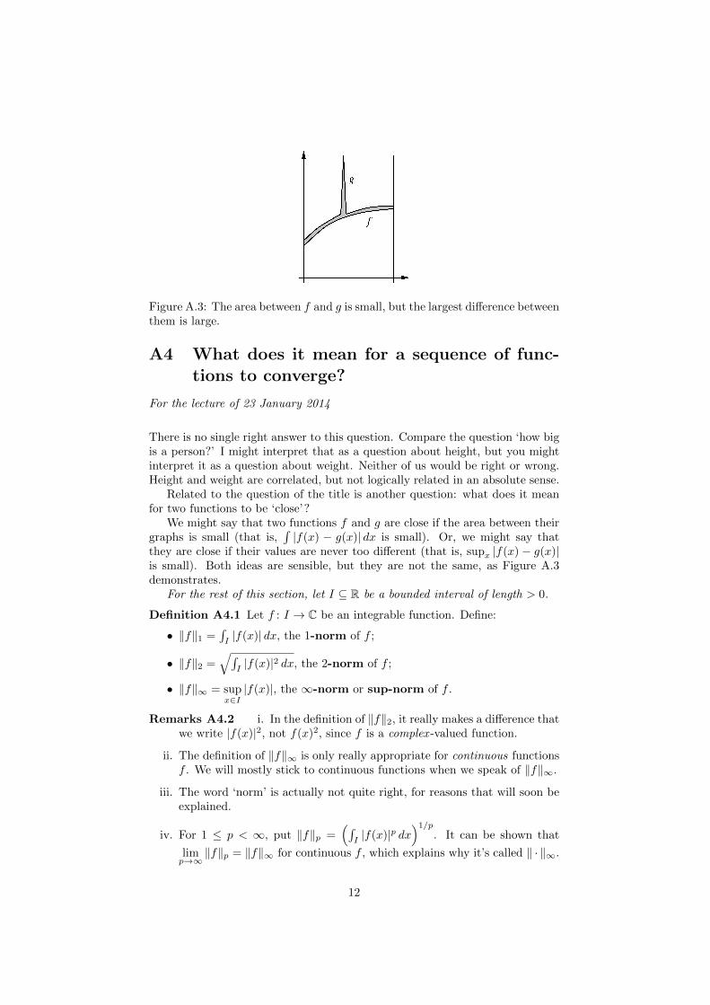
Figure A.3: The area between f and g is small, but the largest difference betweenthem is large.
A4 What does it mean for a sequence of func-tions to converge?
For the lecture of 23 January 2014
There is no single right answer to this question. Compare the question ‘how bigis a person?’ I might interpret that as a question about height, but you mightinterpret it as a question about weight. Neither of us would be right or wrong.Height and weight are correlated, but not logically related in an absolute sense.
Related to the question of the title is another question: what does it meanfor two functions to be ‘close’?
We might say that two functions f and g are close if the area between theirgraphs is small (that is,
∫|f(x) − g(x)| dx is small). Or, we might say that
they are close if their values are never too different (that is, supx |f(x) − g(x)|is small). Both ideas are sensible, but they are not the same, as Figure A.3demonstrates.
For the rest of this section, let I ⊆ R be a bounded interval of length > 0.
Definition A4.1 Let f : I → C be an integrable function. Define:
• ‖f‖1 =∫I|f(x)| dx, the 1-norm of f ;
• ‖f‖2 =√∫
I|f(x)|2 dx, the 2-norm of f ;
• ‖f‖∞ = supx∈I|f(x)|, the ∞-norm or sup-norm of f .
Remarks A4.2 i. In the definition of ‖f‖2, it really makes a difference thatwe write |f(x)|2, not f(x)2, since f is a complex -valued function.
ii. The definition of ‖f‖∞ is only really appropriate for continuous functionsf . We will mostly stick to continuous functions when we speak of ‖f‖∞.
iii. The word ‘norm’ is actually not quite right, for reasons that will soon beexplained.
iv. For 1 ≤ p < ∞, put ‖f‖p =(∫
I|f(x)|p dx
)1/p
. It can be shown that
limp→∞
‖f‖p = ‖f‖∞ for continuous f , which explains why it’s called ‖ · ‖∞.
12
If we want to refer to the 1-norm in the abstract, we sometimes write it as‖ · ‖1. The dot is a blank or placeholder, into which arguments can be inserted.The same goes for ‖ · ‖2 and ‖ · ‖∞.
Lemma A4.3 Let ‖ · ‖ stand for any of ‖ · ‖1, ‖ · ‖2 or ‖ · ‖∞. Then for allintegrable functions f, g : I → C and all c ∈ C:
i. ‖f‖ ≥ 0;
ii. ‖cf‖ = |c| · ‖f‖;
iii. ‖f + g‖ ≤ ‖f‖+ ‖g‖.
Proof All easy except (iii) for ‖ · ‖2, which is Sheet 1, q.6(iv). �
A norm on the set {integrable functions I → C} is an operation satisfyingconditions (i)–(iii) and one further condition: that if ‖f‖ = 0 then f = 0. Thisfurther condition fails for ‖·‖1 and ‖·‖2 (as the next example shows), so strictlyspeaking we should call them ‘seminorms’. But I will abuse terminology and goon calling them the 1-norm and 2-norm. (The ∞-norm really is a norm.)
Example A4.4 Define f : [0, 1)→ C by
f(x) =
{1 if x = 0,
0 otherwise.
Then ‖f‖1 = ‖f‖2 = 0 but f 6= 0.
Lemma A4.5 i. For an integrable function f : I → C,
‖f‖1 = 0 ⇐⇒ f = 0 a.e. ⇐⇒ ‖f‖2 = 0.
ii. For an integrable function f : I → C, if ‖f‖1 = 0 or ‖f‖2 = 0 thenf(x) = 0 for all x ∈ I such that f is continuous at x.
iii. For a continuous function f : I → C,
‖f‖1 = 0 ⇐⇒ f = 0 ⇐⇒ ‖f‖2 = 0.
iv. For an integrable (or just bounded) function f : I → C,
‖f‖∞ = 0 ⇐⇒ f = 0.
Proof i. Follows from Facts A3.13 and A3.14.
ii. Follows from Proposition A3.16(i) (taking h = |f | or h = |f |2).
iii. Follows from (ii).
iv. Follows from the definition. �
We’ve seen that ‖f‖1, ‖f‖2 and ‖f‖∞ are three different measures of thesize of a function f .
So, ‖f − g‖1, ‖f − g‖2 and ‖f − g‖∞ are three different measures of thedistance between functions f and g.
They genuinely measure different things! Look back at the opening para-graphs of this lecture and Figure A.3.
We now consider the three resulting notions of convergence, plus two more.
13
Definition A4.6 Let (fn) be a sequence of integrable functions from I to C,and let f be an integrable function from I to C. We say:
• fn → f in ‖ · ‖1 if ‖fn − f‖1 → 0 as n→∞;
• fn → f in ‖ · ‖2 (or in mean square) if ‖fn − f‖2 → 0 as n→∞;
• fn → f in ‖ · ‖∞ (or uniformly) if ‖fn − f‖∞ → 0 as n→∞;
• fn → f pointwise if for all x ∈ I, fn(x)→ f(x) as n→∞;
• fn → f a.e. if for almost all x ∈ I, fn(x)→ f(x) as n→∞.
All five types of convergence are useful and meaningful.We now work out the logical relationships between them. First, here’s some-
thing in common between the first three.
Lemma A4.7 Let ‖ · ‖ stand for ‖ · ‖1, ‖ · ‖2 or ‖ · ‖∞. If fn → f in ‖ · ‖ then‖fn‖ → ‖f‖ as n→∞.
Proof For all n, we have
‖fn‖ − ‖f‖ ≤ ‖fn − f‖
by Lemma A4.3(iii), and similarly
‖f‖ − ‖fn‖ ≤ ‖f − fn‖ = ‖fn − f‖,
so ∣∣ ‖fn‖ − ‖f‖ ∣∣ ≤ ‖fn − f‖.But ‖fn − f‖ → 0 as n→∞, so ‖fn‖ − ‖f‖ → 0 as n→∞, as required. �
Here’s a classic fact from PAA:
Fact A4.8 Let f, f1, f2, . . . : I → C be functions such that fn → f uniformly.Suppose that each fn is continuous. Then f is continuous, and
∫Ifn(x) dx →∫
If(x) dx as n→∞.
In words: a uniform limit of continuous functions is continuous, and the integralof a uniform limit is the limit of the integrals.
Now let’s begin to record the implications between the different types ofconvergence.
Lemma A4.9 Let f, f1, f2, . . . : I → C be integrable functions. Then
fn → f uniformly
⇒ fn → f pointwise
⇒ fn → f a.e..
Proof Immediate from the definitions. �
We now restrict ourselves to the case I = [0, 1), since that’s what we’ll needonce we start to consider 1-periodic functions.
14
Lemma A4.10 i. Let f : [0, 1)→ C be an integrable function. Then
‖f‖1 ≤ ‖f‖2 ≤ ‖f‖∞.
ii. Let f, f1, f2, . . . : [0, 1)→ C be integrable functions. Then
fn → f in ‖ · ‖∞⇒ fn → f in ‖ · ‖2⇒ fn → f in ‖ · ‖1.
Proof i. We prove ‖f‖1 ≤ ‖f‖2 later. (Reader: fill in the reference oncewe’ve got to it!) For the other inequality:
‖f‖2 =
√∫ 1
0
|f(x)|2 dx ≤
√∫ 1
0
‖f‖2∞ dx = ‖f‖∞.
ii. Follows from (i) (with fn − f in place of f). �
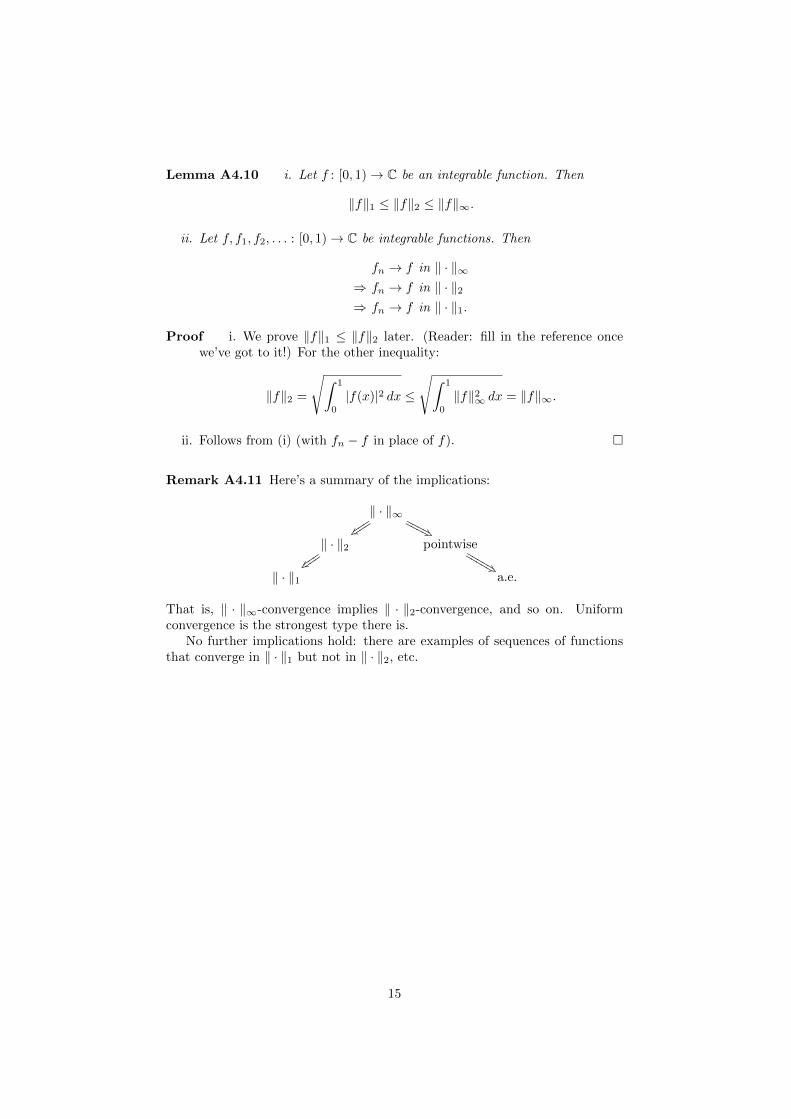
Remark A4.11 Here’s a summary of the implications:
‖ · ‖∞u} tttttt
#+NNNNNNNN
‖ · ‖2v~ uuuuuu
pointwise
"*LLLLLLLLLL
‖ · ‖1 a.e.
That is, ‖ · ‖∞-convergence implies ‖ · ‖2-convergence, and so on. Uniformconvergence is the strongest type there is.
No further implications hold: there are examples of sequences of functionsthat converge in ‖ · ‖1 but not in ‖ · ‖2, etc.
15
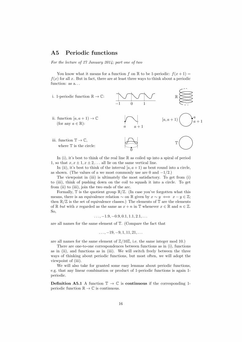
A5 Periodic functions
For the lecture of 27 January 2014; part one of two
You know what it means for a function f on R to be 1-periodic: f(x+ 1) =f(x) for all x. But in fact, there are at least three ways to think about a periodicfunction: as a. . .
i. 1-periodic function R→ C:
−1 0 1
R
ii. function [a, a+ 1)→ C(for any a ∈ R):
a a+ 1
[a, a+ 1)aa+ 1
iii. function T→ C,
where T is the circle:0
T
In (i), it’s best to think of the real line R as coiled up into a spiral of period1, so that x, x± 1, x± 2, . . . all lie on the same vertical line.
In (ii), it’s best to think of the interval [a, a+ 1) as bent round into a circle,as shown. (The values of a we most commonly use are 0 and −1/2.)
The viewpoint in (iii) is ultimately the most satisfactory. To get from (i)to (iii), think of pushing down on the coil to squash it into a circle. To getfrom (ii) to (iii), join the two ends of the arc.
Formally, T is the quotient group R/Z. (In case you’ve forgotten what thismeans, there is an equivalence relation ∼ on R given by x ∼ y ⇐⇒ x− y ∈ Z;then R/Z is the set of equivalence classes.) The elements of T are the elementsof R but with x regarded as the same as x+ n in T whenever x ∈ R and n ∈ Z.So,
. . . ,−1.9,−0.9, 0.1, 1.1, 2.1, . . .
are all names for the same element of T. (Compare the fact that
. . . ,−19,−9, 1, 11, 21, . . .
are all names for the same element of Z/10Z, i.e. the same integer mod 10.)There are one-to-one correspondences between functions as in (i), functions
as in (ii), and functions as in (iii). We will switch freely between the threeways of thinking about periodic functions, but most often, we will adopt theviewpoint of (iii).
We will also take for granted some easy lemmas about periodic functions,e.g. that any linear combination or product of 1-periodic functions is again 1-periodic.
Definition A5.1 A function T → C is continuous if the corresponding 1-periodic function R→ C is continuous.
16
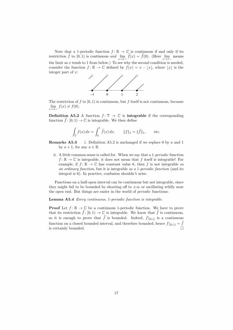
Note that a 1-periodic function f : R → C is continuous if and only if itsrestriction f to [0, 1) is continuous and lim
x→1−f(x) = f(0). (Here lim
x→1−means
the limit as x tends to 1 from below.) To see why the second condition is needed,consider the function f : R → C defined by f(x) = x − bxc, where bxc is theinteger part of x:
10 2−1
The restriction of f to [0, 1) is continuous, but f itself is not continuous, becauselimx→1−
f(x) 6= f(0).
Definition A5.2 A function f : T → C is integrable if the correspondingfunction f : [0, 1)→ C is integrable. We then define∫
Tf(x) dx =
∫ 1
0
f(x) dx, ‖f‖1 = ‖f‖1, etc.
Remarks A5.3 i. Definition A5.2 is unchanged if we replace 0 by a and 1by a+ 1, for any a ∈ R.
ii. A little common sense is called for. When we say that a 1-periodic functionf : R → C is integrable, it does not mean that f itself is integrable! Forexample, if f : R → C has constant value 6, then f is not integrable asan ordinary function, but it is integrable as a 1-periodic function (and itsintegral is 6). In practice, confusion shouldn’t arise.
Functions on a half-open interval can be continuous but not integrable, sincethey might fail to be bounded by shooting off to ±∞ or oscillating wildly nearthe open end. But things are easier in the world of periodic functions:
Lemma A5.4 Every continuous, 1-periodic function is integrable.
Proof Let f : R → C be a continuous 1-periodic function. We have to provethat its restriction f : [0, 1) → C is integrable. We know that f is continuous,
so it is enough to prove that f is bounded. Indeed, f |[0,1] is a continuous
function on a closed bounded interval, and therefore bounded; hence f |[0,1) = fis certainly bounded. �
17
A6 The inner product
For the lecture of 27 January 2014; part two of two
You’re familiar with the scalar product v.w of two vectors v, w ∈ Rn, definedby v.w =
∑i viwi. Sometimes this is written as 〈v, w〉. Perhaps you’re familiar
with the complex version: given v, w ∈ Cn, we put 〈v, w〉 =∑i viwi. There is
also a version for complex-valued functions:
Definition A6.1 Let f, g : T→ C be integrable functions. We define
〈f, g〉 =
∫Tf(x)g(x) dx ∈ C.
In order for this definition to make sense, we need to know that the functionf · g is integrable. Lemmas A3.4(iii) and A3.7 guarantee this.
Lemma A6.2 Let f, g, h : T → C be integrable functions, and let a, b ∈ C.Then:
i. 〈g, f〉 = 〈f, g〉;
ii. 〈af + bg, h〉 = a〈f, h〉+ b〈g, h〉 and 〈f, ag + bh〉 = a〈f, g〉+ b〈f, h〉;
iii. 〈f, f〉 = ‖f‖22 ≥ 0.
Proof Sheet 1, q.6. �
The properties of 〈·, ·〉 stated in this lemma nearly say that it is an innerproduct. All that prevents it from being one is that 〈f, f〉 = 0 does not quiteimply f = 0; it only implies that f = 0 almost everywhere (by Lemma A4.5(i)).However, I will abuse terminology slightly by referring to 〈f, g〉 as the innerproduct of f and g anyway.
Here are some further properties of 〈·, ·〉.
Lemma A6.3 Let f, g : T→ C be integrable functions. Then:
i. ‖f + g‖22 = ‖f‖22 + ‖g‖22 + 2Re〈f, g〉 (‘cosine rule’);
ii. if 〈f, g〉 = 0 then ‖f + g‖22 = ‖f‖22 + ‖g‖22 (‘Pythagoras’).
Proof For (i), use ‖h‖22 = 〈h, h〉. Part (ii) follows immediately. �
Here is the most fundamental result about the inner product.
Theorem A6.4 (Cauchy–Schwarz inequality) Let f, g : T → C be inte-grable functions. Then
|〈f, g〉| ≤ ‖f‖2‖g‖2.
Proof Sheet 1, q.6. �
Note the modulus sign on the left-hand side. Without it, the inequalitywould not even make sense, since 〈f, g〉 is not usually a real number.
From this, we deduce that ‖f + g‖2 ≤ ‖f‖2 + ‖g‖2 (Sheet 1, q.6 again; seealso Lemma A4.3). We also deduce the following, which completes the proof ofLemma A4.10:
18
Lemma A6.5 Let f : [0, 1)→ C be an integrable function. Then ‖f‖1 ≤ ‖f‖2.
Proof Let us apply the Cauchy–Schwarz inequality to |f | and the constantfunction 1. We have
〈|f |, 1〉 = ‖f‖1, ‖ |f | ‖2 = ‖f‖2, ‖1‖2 = 1,
giving ‖f‖1 ≤ ‖f‖2 · 1 = ‖f‖2, as required. �
There is a cousin of the Cauchy–Schwarz inequality that is also useful:
Lemma A6.6 Let f, g : T→ C be integrable functions. Then
|〈f, g〉| ≤ ‖f‖1‖g‖∞.
Proof We have
|〈f, g〉| =∣∣∣∣∫
Tf(x)g(x) dx
∣∣∣∣ ≤ ∫T
∣∣f(x)g(x)∣∣ dx
=
∫T|f(x)| · |g(x)| dx ≤
∫T|f(x)| · ‖g‖∞ dx = ‖f‖1‖g‖∞,
using Lemma A3.9 in the first inequality. �
Remark A6.7 (Non-examinable.) Both the Cauchy–Schwarz inequality andLemma A6.6 are special cases of a result known as Holder’s inequality, whichstates that |〈f, g〉| ≤ ‖f‖p‖g‖q whenever 1/p + 1/q = 1 (with 1 ≤ p ≤ ∞,1 ≤ q ≤ ∞). Here ‖f‖p and ‖g‖q are defined as in Remark A4.2(iv).
Lemma A6.6 easily implies two more small results, both of which will beuseful later:
Lemma A6.8 Let f : T → C be an integrable function. Then ‖f‖2 ≤√‖f‖1‖f‖∞.
Proof Put g = f in Lemma A6.6. �
Lemma A6.9 Let f1, f2, . . . , f, g : T→ C be integrable functions. Suppose thatfn → f as n→∞ in ‖ · ‖1. Then 〈fn, g〉 → 〈f, g〉 as n→∞.
Proof For each n, we have
|〈fn, g〉 − 〈f, g〉| = |〈fn − f, g〉| ≤ ‖fn − f‖1‖g‖∞,
and ‖fn − f‖1 → 0 as n→∞, so the result follows. �
19
A7 Characters and Fourier series
For the lecture of 30 January 2014; part one of two
Among all periodic functions, certain ones are special. These are the so-called ‘characters’. Fourier theory can be seen as an attempt to build all periodicfunctions out of characters.
Let k ∈ Z. We define ek : R → C by ek(x) = e2πikx. This function is1-periodic, so can be seen as a function ek : T→ C, the kth character of T.
Remarks A7.1 i. The notation ek is not standard. No one outside thisclass will know what you mean by ‘ek’ unless you define it.
ii. The apparently strange terminology ‘character of T’ will be put into con-text in the very last part of this course.
Here are some elementary properties of the characters.
Lemma A7.2 Let k ∈ Z and x, y ∈ T. Then:
i. ek is continuous;
ii. |ek(x)| = 1;
iii. ek(x+ y) = ek(x)ek(y), ek(−x) = 1/ek(x), and ek(0) = 1.
Note that in (iii), it does make sense to add and subtract elements of T,because T is by definition a group (the quotient R/Z).
Proof Straightforward. �
Some further elementary properties:
Lemma A7.3 Let k, ` ∈ Z. Then:
i. ek+` = ek · e`, e−k = 1/ek, and e0 = 1;
ii. e−k = ek;
iii. ek = ek1 .
Proof Straightforward. �
We now come to a crucial property of the characters.
Lemma A7.4 The characters (ek)k∈Z are orthonormal. That is, for k, ` ∈ Z,
〈ek, e`〉 =
{1 if k = `,
0 if k 6= `.
Proof We have
〈ek, e`〉 =
∫Tek(x)e`(x) dx =
∫ 1
0
ek(x)e−`(x) dx =
∫ 1
0
ek−`(x) dx,
using Lemma A7.3. If k = ` then the integrand is e0 = 1, so 〈ek, e`〉 = 1. Ifk 6= ` then
〈ek, e`〉 =
[1
2πi(k − `)e2πi(k−`)x
]1
0
= 0,
as required. �
20
You can think of the characters as analogous to the standard basis vectorsin Rn (which are also orthonormal). When we express a point of Rn in terms ofits coordinates, we are viewing it as a linear combination of the standard basisvectors. Similarly, in Fourier theory, we seek to view any periodic function as alinear combination of the characters. The analogy is not exact, because thereare infinitely many characters, so we have to take infinite linear combinationsof characters. This is what gives the subject its subtlety.
Here are the central definitions of this course.
Definition A7.5 Let f : T→ C be an integrable function.
i. For k ∈ Z, the kth Fourier coefficient of f is
f(k) = 〈f, ek〉.
ii. For n ≥ 0, the nth Fourier partial sum of f is the function
Snf =
n∑k=−n
f(k)ek : T→ C.
iii. The Fourier series of f is the expression
Sf =
∞∑k=−∞
f(k)ek.
Remarks A7.6 i. Explicitly,
f(k) =
∫ 1
0
f(x)e−2πikx dx (k ∈ Z),
(Snf)(x) =
n∑k=−n
f(k)e2πikx (n ≥ 0, x ∈ T),
(Sf)(x) =
∞∑k=−∞
f(k)e2πikx.
ii. The Fourier series of f is∑∞k=−∞〈f, ek〉ek. Compare: if u1, . . . , un denote
the standard basis vectors of Rn, then v =∑nk=1(v.uk)uk for all v ∈ Rn.
So, we might guess that f is ‘equal’ to its Fourier series (whatever thatmeans). The central question of this subject is whether, and in what sense,this is actually true.
We finish by recording two basic properties of Fourier coefficients.
Lemma A7.7 Let k ∈ Z. Then:
i. af + bg(k) = af(k) + bg(k) for all a, b ∈ C and integrable f, g : T→ C.
ii. Let f1, f2, . . . , f : T → C be integrable functions such that fn → f as
n→∞ in ‖ · ‖1. Then fn(k)→ f(k) as n→∞.
Proof Part (i) follows from Lemma A6.2, and part (ii) from Lemma A6.9. �
21
A8 Trigonometric polynomials
For the lecture of 30 January 2014; part two of two
As we saw in the last section, Fourier theory asks whether a periodic functionf can be expressed as a linear combination Sf =
∑∞k=−∞ f(k)ek of characters
ek. This is, in general, an infinite linear combination (whatever that means).But to get started, it is useful to consider the finite linear combinations ofcharacters. These are called trigonometric polynomials.
Definition A8.1 A function g : T → C is a trigonometric polynomial ifthere exist n ≥ 0 and c−n, . . . , c0, . . . , cn ∈ C such that g =
∑nk=−n ckek. The
degree of g is the least n for which this is possible.
Example A8.2 For any integrable f : T → C and n ≥ 0, the nth Fourierpartial sum Snf =
∑nk=−n f(k)ek is a trigonometric polynomial of degree ≤ n.
It is perhaps not obvious that the coefficients of a trigonometric polynomialare unique. The next two results show that, in fact, they are.
Lemma A8.3 Let g =∑nk=−n ckek be a trigonometric polynomial. Then
g(k) =
{ck if |k| ≤ n,0 if |k| > n
(k ∈ Z).
Proof We have
g(k) = 〈g, ek〉 =
⟨n∑
`=−n
c`e`, ek
⟩=
n∑`=−n
c`〈e`, ek〉
=
{ck if − n ≤ k ≤ n0 otherwise,
where in the last step we used the fact that the characters are orthonormal. �
Corollary A8.4 If∑nk=−n ckek =
∑nk=−n dkek then ck = dk for all k ∈
{−n, . . . , 0, . . . , n}. �
In other words, the characters are linearly independent.
Example A8.5 Let f : T → C be an integrable function. Then for all n ≥ 0and k ∈ Z,
Snf(k) =
{f(k) if |k| ≤ n,0 otherwise.
In other words, Snf and f have the same kth Fourier coefficients for |k| ≤ n.
22
Here is a baby version of the whole of Fourier theory.
Proposition A8.6 Let n ≥ 0. Then the functions
{trigonometric polynomials of degree ≤ n} � C2n+1
given byg 7→
(g(−n), . . . , g(0), . . . , g(n)
)∑nk=−n ckek ←[ (c−n, . . . , c0, . . . , cn)
are mutually inverse.
Proof • Let g =∑nk=−n ckek be a trigonometric polynomial of degree ≤ n.
We must show that g =∑nk=−n g(k)ek. This follows from Lemma A8.3.
• Let (c−n, . . . , cn) ∈ C2n+1 and put g =∑nk=−n ckek. We must show that
g(k) = ck for all k ∈ {−n, . . . , n}. This also follows from Lemma A8.3. �
Fantasy A8.7 We can fantasize about extending Proposition A8.6 to a pair ofmutually inverse functions
{nice functions T→ C} � {nice double sequences in C}
given by
f 7→(f(k)
)∞k=−∞∑∞
k=−∞ ckek ←[ (ck)∞k=−∞.
The rest of the course explores this fantasy.
23

−t 0
f(·+ t) f
Figure A.4: Translating a function.
A9 Integrable functions are sort of continuous
For the lecture of 3 February 2014
Integrable functions are not necessarily continuous. However, integrablefunctions do satisfy a continuity-like condition of a not-so-obvious kind, as fol-lows.
Let f : T→ C be a function. Given t ∈ T, we obtain a new function
f(·+ t) : T→ C
defined byx 7→ f(x+ t).
Geometrically, this means shifting the graph of the function by t units to theleft (Fig. A.4). (Or really, since T is a circle, it means rotating the graph by afraction t of a revolution.) It’s not so hard to see (try it!) that
f is continuous ⇐⇒ f(·+ t)→ f pointwise as t→ 0
—in other words, for each x ∈ T, f(x+ t)→ f(x) as t→ 0. Similarly, it’s nothard to see that
f is uniformly continuous ⇐⇒ f(·+ t)→ f in ‖ · ‖∞ as t→ 0
—in other words, ‖f(· + t) − f‖∞ → 0 as t → 0. Obviously, neither conditionis satisfied by an arbitrary integrable function. However, it is true that for anyintegrable function,
f(·+ t)→ f in ‖ · ‖1 as t→ 0. (A:4)
Proving this will take the rest of this lecture, and will require us to go rightback to the definition of integrability.
Here’s the plan. First we’ll introduce a class of particularly simple functions,the so-called ‘step functions’. We’ll show that every integrable function canbe closely approximated by a step function. The proof of (A:4) for arbitraryintegrable functions f proceeds in two steps: (i) prove it for step functions(which is relatively easy, as step functions are so simple); (ii) extend the resultto an arbitrary integrable f by approximating it with step functions.
Definition A9.1 Let I ⊆ R be a bounded interval. A step function is afunction f : I → C such that f =
∑nk=1 ckχJk for some n ≥ 0, c1, . . . , cn ∈ C,
and bounded intervals J1, . . . , Jn ⊆ I.
24
0 1 2 3
Figure A.5: A step function.
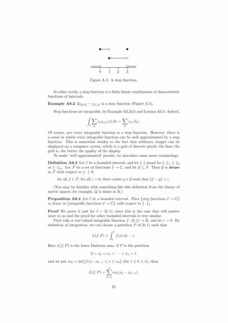
In other words, a step function is a finite linear combination of characteristicfunctions of intervals.
Example A9.2 2χ[0,3] − χ[1,3) is a step function (Figure A.5).
Step functions are integrable, by Example A3.2(ii) and Lemma A3.4. Indeed,∫I
∑k
ckχJk(x) dx =∑k
ck |Jk| .
Of course, not every integrable function is a step function. However, there isa sense in which every integrable function can be well approximated by a stepfunction. This is somewhat similar to the fact that arbitrary images can bedisplayed on a computer screen, which is a grid of discrete pixels; the finer thegrid is, the better the quality of the display.
To make ‘well approximated’ precise, we introduce some more terminology.
Definition A9.3 Let I be a bounded interval, and let ‖ ·‖ stand for ‖ ·‖1, ‖ ·‖2or ‖ · ‖∞. Let F be a set of functions I → C, and let G ⊆ F . Then G is densein F with respect to ‖ · ‖ if:
for all f ∈ F , for all ε > 0, there exists g ∈ G such that ‖f − g‖ < ε.
(You may be familiar with something like this definition from the theory ofmetric spaces; for example, Q is dense in R.)
Proposition A9.4 Let I be a bounded interval. Then {step functions I → C}is dense in {integrable functions I → C} with respect to ‖ · ‖1.
Proof We prove it just for I = [0, 1), since this is the case that will mattermost to us and the proof for other bounded intervals is very similar.
First take a real -valued integrable function f : [0, 1)→ R, and let ε > 0. Bydefinition of integration, we can choose a partition P of [0, 1) such that
L(f, P ) >
∫ 1
0
f(x) dx− ε.
Here L(f, P ) is the lower Darboux sum: if P is the partition
0 = x0 < x1 < · · · < xn = 1
and we put mk = inf{f(x) : xk−1 ≤ x ≤ xk} (for 1 ≤ k ≤ n), then
L(f, P ) =
n∑k=1
mk(xk − xk−1).
25
Put Jk = [xk−1, xk) and put
g =
n∑k=1
mkχJk .
(Draw a picture!) Then g is a step function, with L(f, P ) =∫ 1
0g(x) dx. We
have g(x) ≤ f(x) for all x ∈ [0, 1), so
‖f − g‖1 =
∫ 1
0
(f(x)− g(x)) dx =
∫ 1
0
f(x) dx− L(f, P ) < ε,
as required.Now take an arbitrary integrable function f : [0, 1)→ C, say f = f1+if2 with
f1, f2 : [0, 1) → R. Let ε > 0. By definition of integrability of complex-valuedfunctions (Definition A3.1(i)), f1 and f2 are integrable. So by the previousparagraph, we can choose step functions g1, g2 : [0, 1)→ R such that
‖f1 − g1‖1 < ε/2, ‖f2 − g2‖1 < ε/2.
Put g = g1 + ig2 : [0, 1)→ C, which is also a step function. Then
‖f − g‖1 = ‖(f1 − g1) + i(f2 − g2)‖1 ≤ ‖f1 − g1‖1 + ‖f2 − g2‖1 < ε/2 + ε/2 = ε
(using Lemma A4.3), as required. �
We are now ready to prove that integrable functions are ‘sort of continuous’,in the sense of (A:4), following the plan described above.
Theorem A9.5 Let f : T→ C be an integrable function. Then f(·+ t)→ f in‖ · ‖1 as t→ 0 (that is, ‖f(·+ t)− f‖1 → 0 as t→ 0).
Proof For the duration of this proof only, let us say that an integrable functiong : T → C is ‘good’ if g(· + t) → g in ‖ · ‖1 as t → 0. We will prove that everyintegrable function is good.
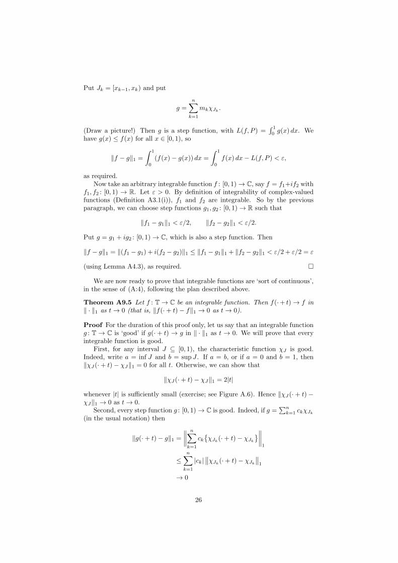
First, for any interval J ⊆ [0, 1), the characteristic function χJ is good.Indeed, write a = inf J and b = sup J . If a = b, or if a = 0 and b = 1, then‖χJ(·+ t)− χJ‖1 = 0 for all t. Otherwise, we can show that
‖χJ(·+ t)− χJ‖1 = 2|t|
whenever |t| is sufficiently small (exercise; see Figure A.6). Hence ‖χJ(·+ t)−χJ‖1 → 0 as t→ 0.
Second, every step function g : [0, 1)→ C is good. Indeed, if g =∑nk=1 ckχJk
(in the usual notation) then
‖g(·+ t)− g‖1 =
∥∥∥∥ n∑k=1
ck{χJk(·+ t)− χJk
}∥∥∥∥1
≤n∑k=1
|ck|∥∥χJk(·+ t)− χJk
∥∥1
→ 0
26
a− t a b− t b
Figure A.6: The area between a characteristic function and a translation of itby a small distance t is 2|t|.
as t→ 0, by the first part.Finally, every integrable function f : [0, 1) → C is good. Indeed, let ε > 0.
By Proposition A9.4, we can choose a step function g : [0, 1) → C such that‖f − g‖1 < ε/3. This implies that for all t ∈ R,
‖f(·+ t)− g(·+ t)‖1 =
∫T|f(x+ t)− g(x+ t)| dx
=
∫T|f(y)− g(y)| dy = ‖f − g‖1 < ε/3,
where the second equality is by substitution. (Intuitively, the area between thegraphs f and g is unchanged if we shift everything horizontally by t.) Also,by the second part, we can choose δ > 0 such that for all t ∈ (−δ, δ), we have‖g(·+ t)− g‖1 < ε/3. Now for all t ∈ (−δ, δ), we have
‖f(·+ t)− f‖1 ≤ ‖f(·+ t)− g(·+ t)‖1 + ‖g(·+ t)− g‖1 + ‖g − f‖1< ε/3 + ε/3 + ε/3 = ε,
as required. �
27
Chapter B
Convergence of Fourierseries in the 2- and 1-norms
In this chapter, we’ll prove:
for any integrable function f : T → C, the Fourier series of f con-verges to f in both ‖ · ‖2 and ‖ · ‖1.
It’s as simple as that. Compare the long and complicated saga of pointwiseconvergence recounted in Section A2. In contrast, this result is clean, easilystated, and not too difficult to prove.
The 2-norm will play a much greater role than the 1-norm in this chapter. Be-cause ‖·‖2 goes hand in hand with inner products (recalling that ‖f‖22 = 〈f, f〉),working in the 2-norm has a great deal in common with ordinary Euclidean ge-ometry. It’s the most easily visualized context to work in.
B1 Nothing is better than a Fourier partial sum
For the lecture of 6 February 2014; part one of two
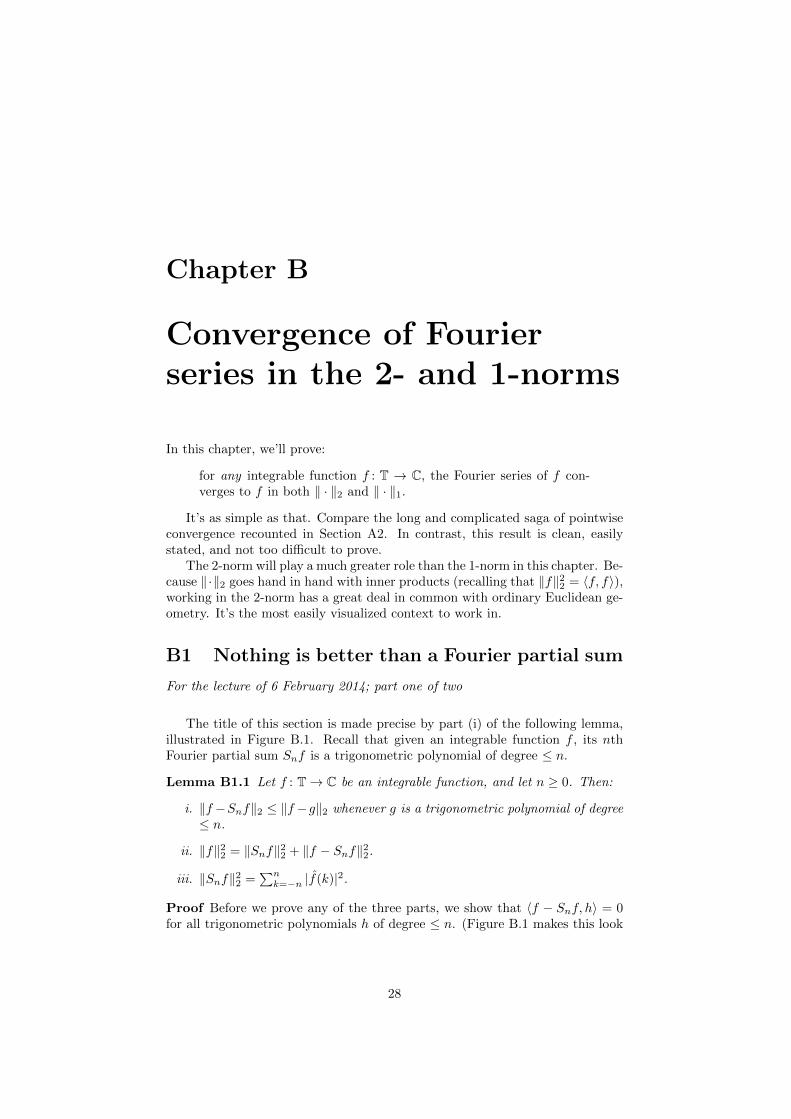
The title of this section is made precise by part (i) of the following lemma,illustrated in Figure B.1. Recall that given an integrable function f , its nthFourier partial sum Snf is a trigonometric polynomial of degree ≤ n.
Lemma B1.1 Let f : T→ C be an integrable function, and let n ≥ 0. Then:
i. ‖f−Snf‖2 ≤ ‖f−g‖2 whenever g is a trigonometric polynomial of degree≤ n.
ii. ‖f‖22 = ‖Snf‖22 + ‖f − Snf‖22.
iii. ‖Snf‖22 =∑nk=−n |f(k)|2.
Proof Before we prove any of the three parts, we show that 〈f − Snf, h〉 = 0for all trigonometric polynomials h of degree ≤ n. (Figure B.1 makes this look
28

f
Snf
0
g
trig polys of deg ≤ n
Figure B.1: Approximating a function f by a trigonometric polynomial of degree≤ n.
plausible.) Indeed, by linearity, it is enough to prove this when h = ek for somek ∈ {−n, . . . , 0, . . . , n}, and
〈f − Snf, ek〉 = 〈f, ek〉 − 〈Snf, ek〉 = f(k)− Snf(k) = 0
by Example A8.5, as required.Now let g be a trigonometric polynomial of degree ≤ n. By what we have
just shown, 〈f − Snf, Snf − g〉 = 0, so
‖f − g‖22 = ‖(f − Snf) + (Snf − g)‖22= ‖f − Snf‖22 + ‖Snf − g‖22 (B:1)
by Pythagoras (Lemma A6.3(ii)). Part (i) follows, then part (ii) by puttingg = 0 in (B:1).
For part (iii), we have
‖Snf‖22 =
⟨n∑
k=−n
f(k)ek,
n∑`=−n
f(`)el
⟩
=
n∑k,`=−n
f(k)f(`)〈ek, e`〉
=
n∑k=−n
∣∣∣f(k)∣∣∣2 ,
where the first two equalities use Lemma A6.2 and the third uses the orthonor-mality of the characters (Lemma A7.4). �
To elaborate a little on the title of this section: among all trigonometricpolynomials of degree ≤ n, nothing approximates f better than the Fourierpartial sum Snf .
Proposition B1.2 Let f : T→ C be an integrable function. Then:
i.∑∞k=−∞
∣∣f(k)∣∣2 converges; indeed,
∑∞k=−∞
∣∣f(k)∣∣2 ≤ ‖f‖22.
ii. (Riemann–Lebesgue Lemma) f(k)→ 0 as k → ±∞.
29
Proof By parts (ii) and (iii) of Lemma B1.1, we have∑nk=−n |f(k)|2 ≤ ‖f‖22
for all n ≥ 0. The results follow. �
The Riemann–Lebesgue lemma tells us that not every double sequence(ck)∞k=−∞ of complex numbers arises as the sequence of Fourier coefficients ofsome function. This is already a substantial result. Looking back again atFantasy A8.7, we begin to get a sense of what a ‘nice’ double sequence mightbe.
The next lemma will help us to prove that (Snf) always converges to f inthe 2-norm.
Lemma B1.3 Let f : T→ C be an integrable function. The following are equiv-alent:
i. Snf → f in ‖ · ‖2;
ii. gn → f in ‖ · ‖2 for some sequence (gn) of trigonometric polynomials.
Proof (i) ⇒ (ii) is trivial, since each Snf is a trigonometric polynomial.For (ii) ⇒ (i), let ε > 0. Choose m such that ‖f − gm‖2 < ε. Put N =
deg(gm). Thenε > ‖f − gm‖2 ≥ ‖f − SNf‖2,
using Lemma B1.1(i) in the second inequality. But then
‖f − SNf‖2 ≥ ‖f − SN+1f‖2
by Lemma B1.1(i) again, noting that SNf has degree ≤ N + 1. Continuing likethis, we find that
ε > ‖f − SNf‖2 ≥ ‖f − SN+1f‖2 ≥ ‖f − SN+2f‖2 ≥ · · · ,
and in particular, ‖f − Snf‖2 < ε for all n ≥ N . �
Our strategy for proving that Snf → f in ‖ · ‖2 will be to prove that gn → fin ‖ · ‖2 for some other sequence (gn) of trigonometric polynomials—a sequencethat is easier to work with than (Snf) itself.
In order to carry out this strategy, we need to come up with some convenientsequence (gn) of trigonometric polynomials. How can we cook up new trigono-metric polynomials? By convolution, as we’ll see in the next two sections.
30

B2 Convolution: definition and examples
For the lecture of 6 February 2014; part two of two
You’ve already met convolution of functions on R. Convolution of functionson T, which is what we’ll mostly be concerned with, is very similar.
Definition B2.1 Let f, g : T → C be integrable functions. The convolutionf ∗ g : T→ C is the function defined by
(f ∗ g)(x) =
∫Tf(t)g(x− t) dt
(x ∈ T).
Remark B2.2 Recall from Section A5 that the circle T is a group (the quotientR/Z). The group operation is addition mod 1. So, it does make sense to addand subtract elements of T, as we did in the definition of convolution.
Our first example of convolution is important enough to be stated as alemma.
Lemma B2.3 For any k ∈ Z and integrable function f : T→ C,
f ∗ ek = 〈f, ek〉ek = f(k)ek.
Proof For all x ∈ T,
(f ∗ ek)(x) =
∫Tf(t)ek(x− t) dt
=
∫Tf(t)ek(x)ek(−t) dt
= ek(x)
∫Tf(t)ek(t) dt
= 〈f, ek〉ek(x)
= f(k)ek(x)
by Lemmas A7.2 and A7.3. �
This is remarkable. It tells us that when we convolve a character ek withanything (anything! ), the result is a scalar multiple of ek. This is a very specialproperty of the characters.
Convolution has a smoothing effect. For the purposes of the following ex-ample, let us consider functions on R rather than T.
Example B2.4 Given an integrable function f : R→ C, we have
(f ∗ χ[−1/2,1/2]
)(x) =
∫ x+1/2
x−1/2
f(t) dt.
This is a ‘moving average’ of f : the value of f ∗ χ[−1/2,1/2] at x is the meanvalue of f over the interval [x− 1/2, x+ 1/2] (Figure B.2).
31
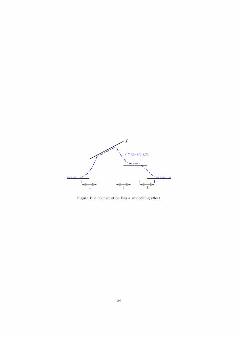
f
f ∗ χ[−1/2,1/2]
1 1 1
Figure B.2: Convolution has a smoothing effect.
32
B3 Convolution: properties
For the lecture of 10 February 2014; part one of two
Example B2.4 showed the smoothing effect of convolution. In that particularexample, the convolution of two discontinuous functions was continuous. Thissurprising behaviour is, in fact, a completely general phenomenon:
Lemma B3.1 Let f, g : T→ C be integrable functions. Then their convolutionf ∗ g : T→ C is continuous.
This is far stronger than we might have guessed in advance. It’s not merelytrue that the convolution of two integrable functions is integrable, or that theconvolution of two continuous functions is continuous. In fact, for any twointegrable functions f and g, no matter how discontinuous they may be, f ∗ gis continuous.
Proof Let x, h ∈ T. Then
|(f ∗ g)(x+ h)− (f ∗ g)(x)| =∣∣∣∣∫
Tf(t)[g(x+ h− t)− g(x− t)] dt
∣∣∣∣≤∫T|f(t)| |g(x+ h− t)− g(x− t)| dt (B:2)
≤ ‖f‖∞∫T|g(x+ h− t)− g(x− t)| dt
= ‖f‖∞∫T|g(u+ h)− g(u)| du (B:3)
= ‖f‖∞ ‖g(·+ h)− g‖1→ 0 as h→ 0. (B:4)
Here (B:2) is by the triangle inequality for integration (Lemma A3.9), equa-tion (B:3) comes from substituting u = x − t, and (B:4) is by Theorem A9.5(‘integrable functions are sort of continuous’). �
Here are some basic properties of convolution. In future, we will use themwithout explicitly referring back to this lemma.
Lemma B3.2 Let f, g, h : T→ C be integrable functions, and let c ∈ C. Then:
i. f ∗ g = g ∗ f ;
ii. (f ∗ g) ∗ h = f ∗ (g ∗ h);
iii. f ∗ (g + h) = (f ∗ g) + (f ∗ h);
iv. f ∗ (cg) = c(f ∗ g).
Proof For (i), let x ∈ T. Then
(f ∗ g)(x) =
∫Tf(t)g(x− t) dt
=
∫Tf(x− u)g(u) du
= (g ∗ f)(x),
by substituting u = x− t. The other parts are similarly straightforward. �
33
Remark B3.3 This lemma tells us that + and ∗ give the set
{integrable functions T→ C}
the structure of a ‘commutative algebra’ over C, that is, both a vector spaceover C and a ring.
Or nearly. The only missing part is that it has no multiplicative identity.Nowadays, the definition of ‘ring’ is usually taken to include the existence of amultiplicative identity; but in analysis especially, there are important rings thatdo not have one.
We’ll see very soon that if the identity did exist, it would be the mythical‘delta function’.
Lemma B3.4 Let f : T → C be an integrable function, and let g : T → C be atrigonometric polynomial. Then f ∗ g is a trigonometric polynomial.
Again, this is stronger than might be expected. It’s not merely true thatthe convolution of two trigonometric polynomials is a trigonometric polyno-mial. In fact, the convolution of anything with a trigonometric polynomial is atrigonometric polynomial.
Proof We may write g =∑nk=−n ckek for some n ≥ 0 and ck ∈ C. Then
f ∗ g =
n∑k=−n
ck(f ∗ ek) =
n∑k=−n
(ckf(k)
)ek,
which is a trigonometric polynomial. Here the second equality usesLemma B2.3. �
Remark B3.5 This lemma says that {trigonometric polynomials} is an idealin the ring {integrable functions T→ C}.
Example B3.6 Every Fourier partial sum of a function f is a convolution off with a trigonometric polynomial. More exactly, using Lemma B2.3 again,
Snf =
n∑k=−n
f(k)ek =
n∑k=−n
f ∗ ek = f ∗n∑
k=−n
ek.
Since∑nk=−n ek is a trigonometric polynomial, Lemma B3.4 tells us in this case
that Snf is also a trigonometric polynomial—which of course we already knew.
Since Fourier partial sums are important in Fourier theory, this examplesuggests that
∑nk=−n ek is also important. It is, and it has its own name:
Definition B3.7 Let n ≥ 0. The Dirichlet kernel of order n is Dn =∑nk=−n ek.
So, Example B3.6 can be restated as:
Lemma B3.8 Snf = f ∗Dn, for all integrable f : T→ C and n ≥ 0. �
Remark B3.9 We can dream of taking n → ∞ in Lemma B3.8, so thatSf = f ∗ D∞ where D∞ =
∑∞k=−∞ ek. However, the sum
∑∞k=−∞ ek does
not converge anywhere, so D∞ does not really exist.
34
Here are two further properties of convolution.
Lemma B3.10 For integrable functions f, g : T→ C,
‖f ∗ g‖∞ ≤ ‖f‖∞‖g‖1.
Proof For all x ∈ T,
|(f ∗ g)(x)| =∣∣∣∣∫
Tf(x− t)g(t) dt
∣∣∣∣≤∫T|f(x− t)| |g(t)| dt
≤ ‖f‖∞∫T|g(t)| dt = ‖f‖∞‖g‖1. �
The final property should remind you of an important fact about Fouriertransforms.
Lemma B3.11 Let f, g : T→ C be integrable functions, and let k ∈ Z. Then
f ∗ g(k) = f(k)g(k).
Proof Sheet 2, q.5. �
35

−ε/2 ε/2
1/ε
Figure B.3: Approximation to the mythical delta function.
B4 The mythical delta function
For the lecture of 10 February 2014; part two of two
This short section is largely intended as motivation for the rest of Part B. Itcontains no definitions or theorems, but the ideas are important for what follows.
Fact: there is no integrable function δ : T→ C such that
for all continuous f : T→ C,∫Tf(x)δ(x) dx = f(0). (B:5)
(Compare Sheet 1, q.5.) But we can get close. Non-rigorously, for a ‘small’ε > 0, put
∆ε =1
εχ[−ε/2,ε/2] : [−1/2, 1/2)→ C
(Figure B.3). Then for any continuous function f : T→ C,∫Tf(x)∆ε(x) dx =
1
ε
∫ ε/2
−ε/2f(x) dx ≈ 1
ε
∫ ε/2
−ε/2f(0) dx = f(0),
using continuity in the approximate equality.Imagine now that there is a function δ satisfying (B:5).Let f : T→ C be a continuous function. Then
f ∗ δ = f,
since
(f ∗ δ)(x) =
∫Tf(x− t)δ(t) dt = f(x− 0) = f(x)
for all x ∈ T. (So δ is an identity for convolution with continuous functions;compare Remark B3.3.)
If δ was actually a trigonometric polynomial, then the equation f ∗ δ = ftogether with Lemma B3.4 would imply that every continuous function f wasa trigonometric polynomial. This is obviously false.
36
If δ is merely a limit of trigonometric polynomials Kn, say Kn → δ in ‖ · ‖2,then perhaps it follows that f ∗Kn → f ∗ δ in ‖ · ‖2. In that case, we would havef ∗Kn → f in ‖ · ‖2. Lemma B1.3 would then imply that Snf → f in ‖ · ‖2.This is the result we’re aiming for.
We know that no δ satisfying (B:5) exists. However, the previous paragraphsuggests a strategy:
Look for a sequence (Kn) of trigonometric polynomials such thatfor all continuous (or even integrable) functions f : T→ C,f ∗Kn → f in ‖ · ‖2.
Our fantasies about the delta function suggest that the sequence (Kn) shouldsomehow ‘converge to δ’. So, the plan now is to look for such a sequence (Kn),and show that it does what this informal chain of reasoning leads us to hope itwill.
37
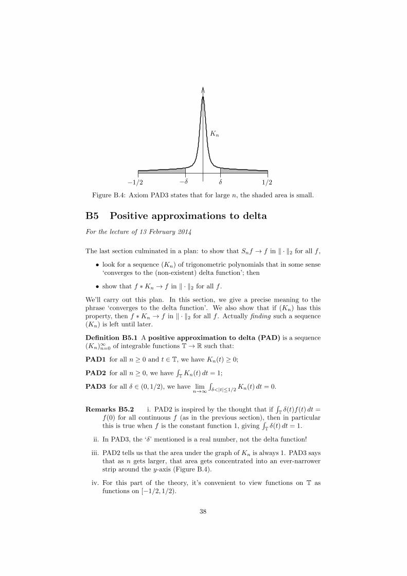
−1/2 1/2−δ δ
Kn
Figure B.4: Axiom PAD3 states that for large n, the shaded area is small.
B5 Positive approximations to delta
For the lecture of 13 February 2014
The last section culminated in a plan: to show that Snf → f in ‖ · ‖2 for all f ,
• look for a sequence (Kn) of trigonometric polynomials that in some sense‘converges to the (non-existent) delta function’; then
• show that f ∗Kn → f in ‖ · ‖2 for all f .
We’ll carry out this plan. In this section, we give a precise meaning to thephrase ‘converges to the delta function’. We also show that if (Kn) has thisproperty, then f ∗Kn → f in ‖ · ‖2 for all f . Actually finding such a sequence(Kn) is left until later.
Definition B5.1 A positive approximation to delta (PAD) is a sequence(Kn)∞n=0 of integrable functions T→ R such that:
PAD1 for all n ≥ 0 and t ∈ T, we have Kn(t) ≥ 0;
PAD2 for all n ≥ 0, we have∫TKn(t) dt = 1;
PAD3 for all δ ∈ (0, 1/2), we have limn→∞
∫δ<|t|≤1/2
Kn(t) dt = 0.
Remarks B5.2 i. PAD2 is inspired by the thought that if∫T δ(t)f(t) dt =
f(0) for all continuous f (as in the previous section), then in particularthis is true when f is the constant function 1, giving
∫T δ(t) dt = 1.
ii. In PAD3, the ‘δ’ mentioned is a real number, not the delta function!
iii. PAD2 tells us that the area under the graph of Kn is always 1. PAD3 saysthat as n gets larger, that area gets concentrated into an ever-narrowerstrip around the y-axis (Figure B.4).
iv. For this part of the theory, it’s convenient to view functions on T asfunctions on [−1/2, 1/2).
38
v. The name ‘approximation to delta’ is non-standard. The usual name is‘approximation to the identity’, since delta is the (non-existent) identityfor convolution.
vi. Almost every definition in this course is conceptually well-motivated. Thisone, however, is not. The conditions PAD1–3 are just what is needed inorder to make the arguments work. (Other variants are possible.) How-ever, it’s only a stepping stone, which we’ll use to reach theorems that areclean and free of arbitrary conditions.
Examples B5.3 i.(nχ[−1/2n,1/2n)
)∞n=1
is a PAD. (Check!) A typical ele-ment of this sequence is shown in Figure B.3, taking ε = 1/n.
ii. (Dn)∞n=0 is not a PAD. First, it fails PAD1, since (for instance) D1(1/2) =−1 < 0. More seriously, it can be shown that ‖Dn‖1 → ∞ as n → ∞,whereas if (Kn) is a PAD then
‖Kn‖1 =
∫TKn(t) dt = 1 (B:6)
for all n (by PAD1 and PAD2).
The rest of this section is devoted to showing that when (Kn) is a PAD,f ∗Kn → f in ‖ · ‖2 for any integrable f . The proof is quite delicate.
The first step is to prove the weaker result that f ∗Kn → f in ‖ · ‖1. (Tosee why it’s ‘weaker’, recall Lemma A4.10.)
Proposition B5.4 Let (Kn)∞n=0 be a PAD and let f : T → C be an integrablefunction. Then f ∗Kn → f in ‖ · ‖1.
Proof We begin by finding an upper bound for ‖f ∗Kn − f‖1.For all x ∈ T and n ≥ 0,
|(f ∗Kn)(x)− f(x)| =∣∣∣∣∫ 1/2
−1/2
(f(x− t)− f(x))Kn(t) dt
∣∣∣∣≤∫ 1/2
−1/2
|f(x− t)− f(x)|Kn(t) dt,
using PAD2 in the first line and PAD1 in the second.(The idea now is roughly as follows. Let δ > 0 be small. Then |f(x−t)−f(x)|
is small for |t| < δ, at least if f is sort of continuous. Also, Kn(t) is small for|t| > δ, since Kn is something like the delta function.)
It follows that for all x ∈ T, n ≥ 0 and δ ∈ (0, 1/2),
|(f ∗Kn)(x)− f(x)|
≤∫|t|<δ
|f(x− t)− f(x)|Kn(t) dt+
∫δ<|t|≤1/2
|f(x− t)− f(x)|Kn(t) dt,
so by the triangle inequality,
|(f ∗Kn)(x)− f(x)|
≤∫|t|<δ
|f(x− t)− f(x)|Kn(t) dt+ 2‖f‖∞∫δ<|t|≤1/2
Kn(t) dt. (B:7)
39
Integrating (B:7) with respect to x shows that for all n ≥ 0 and δ ∈ (0, 1/2),
‖f ∗Kn − f‖1
≤∫ 1/2
−1/2
∫|t|<δ
|f(x− t)− f(x)|Kn(t) dt dx+ 2‖f‖∞∫δ<|t|≤1/2
Kn(t) dt (B:8)
=
∫|t|<δ
‖f(· − t)− f‖1Kn(t) dt+ 2‖f‖∞∫δ<|t|≤1/2
Kn(t) dt. (B:9)
(To get (B:8), we used the fact that 2‖f‖∞∫δ<|t|≤1/2
Kn(t) dt is independent of
x, so that integrating it with respect to x over an interval of length 1 leaves itunchanged.)
We now prove convergence. Let ε > 0. By Theorem A9.5 (‘integrablefunctions are sort of continuous’), we can choose δ ∈ (0, 1/2) such that for allt ∈ (−δ, δ), ‖f(· − t) − f‖1 < ε/2. By PAD3, we can then choose N ≥ 0 suchthat for all n ≥ N , ∫
δ<|t|≤1/2
Kn(t) dt <ε
4‖f‖∞.
So by (B:9), for all n ≥ N ,
‖f ∗Kn − f‖1 ≤ε
2
∫|t|<δ
Kn(t) dt+ 2‖f‖∞ε
4‖f‖∞
≤ ε
2
∫ 1/2
−1/2
Kn(t) dt+ε
2(B:10)
= ε, (B:11)
using PAD1 in (B:10) and PAD2 in (B:11). �
We now know that f ∗Kn → f in ‖ · ‖1 for any integrable f . It is relativelyeasy to deduce the stronger result that f ∗ Kn → f in ‖ · ‖2. The key isLemma A6.8, which gives an upper bound on the 2-norm in terms of the 1- and∞-norms.
Proposition B5.5 Let (Kn)∞n=0 be a PAD and let f : T → C be an integrablefunction. Then f ∗Kn → f in ‖ · ‖2.
Proof For all n ≥ 0, we have
‖f ∗Kn‖∞ ≤ ‖f‖∞‖Kn‖1 = ‖f‖∞
by Lemma B3.10 and (B:6). So for all n ≥ 0,
‖f ∗Kn − f‖∞ ≤ ‖f ∗Kn‖∞ + ‖f‖∞ ≤ 2‖f‖∞.
(Idea: we now have control over the ∞-norm of (f ∗ Kn − f). The previousproposition gives us control over its 1-norm. Putting them together will give uscontrol over its 2-norm.)
Hence for all n ≥ 0, using Lemma A6.8 and Proposition B5.4,
‖f ∗Kn − f‖2 ≤√‖f ∗Kn − f‖1 ‖f ∗Kn − f‖∞
≤√‖f ∗Kn − f‖1
√2‖f‖∞
→ 0 as n→∞. �
40
B6 Summing the unsummable
For the lecture of Monday 24 February 2014
Before I explain the title, recall: we’re looking for a sequence K0,K1, . . . oftrigonometric polynomials that approximate the mythical δ function increas-ingly well.
How can we find one?
Idea If δ existed, its Fourier coefficients would be given by
δ(k) =
∫Tδ(t)e−2πikt dt = e−2πik0 = 1
for all k ∈ Z, and so Snδ =∑nk=−n ek = Dn. If also Snδ → δ as n → ∞, then
Dn → δ. Since Dn is a trigonometric polynomial, we might try Kn = Dn.
Problem (Dn) is not a PAD, as noted in Example B5.3(ii). Also, the sequence(Dn)∞n=0 does not converge in any of our usual five senses. In other words,∑∞k=−∞ ek is thoroughly unsummable.
So, we want to be able to sum unsummable series. This sounds impossible,but it’s not: you just need to be more generous about what ‘summable’ means.To explain this, it’s useful to step back from our particular problem—indeed,step back from Fourier analysis entirely—and think about the general question:how can we sum a divergent series?
Example B6.1 The series
∞∑n=0
(−1)n = 1− 1 + 1− 1 + · · ·
does not converge, since the partial sums SN =∑Nn=0(−1)n are
S0 = 1, S1 = 0, S2 = 1, S3 = 0, . . . ,
and the sequence (SN ) does not converge.Nevertheless, there are non-rigorous ways of evaluating S =
∑∞n=0(−1)n.
For instance:
i. Alice thinks that
S = (1 +−1) + (1 +−1) + (1 +−1) + · · · = 0 + 0 + 0 + · · · = 0.
Bob thinks that
S = 1 + (−1 + 1) + (−1 + 1) + · · · = 1 + 0 + 0 + · · · = 1.
Alice and Bob agree to split the difference, and so conclude that S = 1/2.
41
ii. Consider two copies of S lined up in columns:
2S = (1− 1 + 1− 1 + · · · )+ (1− 1 + 1− · · · )
= 1 + 0 + 0 + 0 + · · ·= 1.
So S = 1/2, the same answer as obtained by Alice and Bob.
iii. Apply the formula for the sum of a geometric series (even though it’sinvalid, as that formula requires the ratio to have modulus strictly lessthan 1):
S =1
1− (−1)= 1/2.
Again, this is the same answer.
Those three methods were just for fun. Each of them can actually be maderespectable, but I won’t show you how. Instead, here’s a fourth way, which isthe one that will matter to us the most.
iv. The sequence of partial sums (1, 0, 1, 0, . . .) doesn’t converge, but it oscil-lates evenly around 1/2. The centre of mass is 1/2, if you like. Since acentre of mass (or centroid) is a mean, this suggests considering the meanof all the partial sums so far.
Put
AN =1
N + 1(S0 + · · ·+ SN ).
A short calculation shows that
AN =
{12 + 1
2(N+1) if N is even,12 if N is odd.
So limN→∞AN = 1/2, as expected.
There is some general terminology for this fourth method.
Definition B6.2 i. Let (sn)∞n=0 be a sequence in C. Its Nth Cesaro mean(N ≥ 0) is
aN =1
N + 1(s0 + · · ·+ sN ) ∈ C.
If aN → s as N →∞, we say that s is the Cesaro limit of (sn).
ii. The Cesaro sum of a series∑∞n=0 xn is the Cesaro limit of the partial
sums SN =∑Nn=0 xn, if it exists.
We have just seen an example of a series that is Cesaro-summable but notsummable in the usual sense. Now we show that the method of Cesaro sum-mation extends the method of ordinary summation, in the sense that if theordinary sum exists then so does the Cesaro sum, and the two sums agree.
Proposition B6.3 i. Let (sn)∞n=0 be a sequence in C, and let s ∈ C. If s isthe limit of (sn) then s is also the Cesaro limit of (sn).
42
ii. Let∑∞n=0 xn be a series in C. If the sum exists, then the Cesaro sum
exists and is equal to∑xn.
Proof We prove (i); then (ii) follows immediately.Let aN be the Nth Cesaro mean of (sn). For all N ≥ 0,
|aN − s| =∣∣∣∣ (s0 − s) + · · ·+ (sN − s)
N + 1
∣∣∣∣ ≤ |s0 − s|+ · · ·+ |sN − s|N + 1
.
(The idea now: we want |aN −s| to be small. Let L be a large integer. Then
|sn − s| is small when n ≥ L, and |s0−s|+···+|sL−1−s|N+1 is small when N is much
greater than L, since the numerator does not depend on N .)Let ε > 0. Since sn → s, we can choose L such that |sn − s| < ε/2 for all
n ≥ L. We can then choose an integer
M ≥ max{L,
2
ε
(|s0 − s|+ · · ·+ |sL−1 − s|
)− 1}.
For all N ≥M ,
|aN − s| ≤|s0 − s|+ · · ·+ |sL−1 − s|
N + 1+|sL − s|+ · · ·+ |sN − s|
N + 1
<(ε/2)(M + 1)
N + 1+
(N − L+ 1)(ε/2)
N + 1(B:12)
≤ (ε/2) + (ε/2) = ε,
where in (B:12), we used the definition of M in the first summand and thedefinition of L in the second. �
Remark B6.4 The partial sums Dn =∑nk=−n ek are too wild to form a PAD.
The proposition we have just proved suggests that the Cesaro means 1N+1 (D0 +
· · ·+DN ) might be tamer. It turns out that they are; indeed, they form a PAD.This will allow us to complete the plan described at the beginning of Section B5,thus proving that in the 2-norm, Fourier series always converge.
43
B7 The Fejer kernel
For the lecture of Thursday 27 February 2014; part one of two
At the end of the last section, we expressed the hope that although the Dirichletkernels Dn do not form a PAD, perhaps their Cesaro means
1
n+ 1(D0 + · · ·+Dn)
do. Here we show that this is indeed the case.
Definition B7.1 Let n ≥ 0. The Fejer kernel of order n is
Fn =1
n+ 1(D0 + · · ·+Dn) : T→ C.
Note that the Fejer kernel, like the Dirichlet kernel, is a trigonometric poly-nomial.
Way back in Section A1, we abandoned the sine-and-cosine formulation ofFourier series, choosing to work with the more elegant exponential formulation.But it will be useful to have expressions for Dn and Fn in traditional trigono-metric form.
Lemma B7.2 Let n ≥ 0 and 0 6= t ∈ T. Then
Dn(t) =sin((2n+ 1)πt)
sinπt, Fn(t) =
1
n+ 1
sin2((n+ 1)πt)
sin2 πt.
Proof We have
Dn(t) =
n∑k=−n
e1(t)k.
Since t 6= 0, we have e1(t) 6= 1, and we may therefore apply the formula forsumming a geometric series. After some routine algebra, we get
Dn(t) =e1(t)n+1/2 − e1(t)−(n+1/2)
e1(t)1/2 − e1(t)−1/2. (B:13)
Noting that e1(t)α = e2πiαt and applying the formula eiθ = cos θ + i sin θ, weobtain the result on Dn(t).
We now use a trick: multiply the top and bottom of (B:13) by the bottom.This gives
Dn(t) =
[e1(t)n+1/2 − e1(t)−(n+1/2)
][e1(t)1/2 − e1(t)−1/2
][e1(t)1/2 − e1(t)−1/2
]2=
[e1(t)n+1 + e1(t)−(n+1)
]−[e1(t)n + e1(t)−n
][e1(t)1/2 − e1(t)−1/2
]2 .
44
So for any N ≥ 0, the sum∑Nn=0Dn(t) telescopes, giving
N∑n=0
Dn(t) =
[e1(t)N+1 + e1(t)−(N+1)
]−[e1(t)0 + e1(t)−0
][e1(t)1/2 − e1(t)−1/2
]2=
[e1(t)(N+1)/2 − e1(t)−(N+1)/2
]2[e1(t)1/2 − e1(t)−1/2
]2=
[2i sin((N + 1)πt)]2
[2i sin(πt)]2,
hence the result on FN (t). �
This explicit formula helps us to prove our main result on the Fejer kernel.
Proposition B7.3 (Fn)∞n=0 is a PAD. In particular, there is a PAD consistingof trigonometric polynomials.
Proof PAD1: By Lemma B7.2, FN (t) ≥ 0 for all N and t.PAD2: First,
∫TDn(t) dt = 1 for all n, since∫TDn(t) dt = 〈Dn, e0〉 =
n∑k=−n
〈ek, e0〉 = 1.
Hence ∫TFN (t) dt =
1
N + 1
(∫T
D0(t) dt+ · · ·+∫TDN (t) dt
)=
1
N + 1(1 + · · ·+ 1) = 1.
PAD3: Let δ ∈ (0, 1/2). We must prove that
limn→∞
∫δ<|t|<1/2
FN (t) dt = 0.
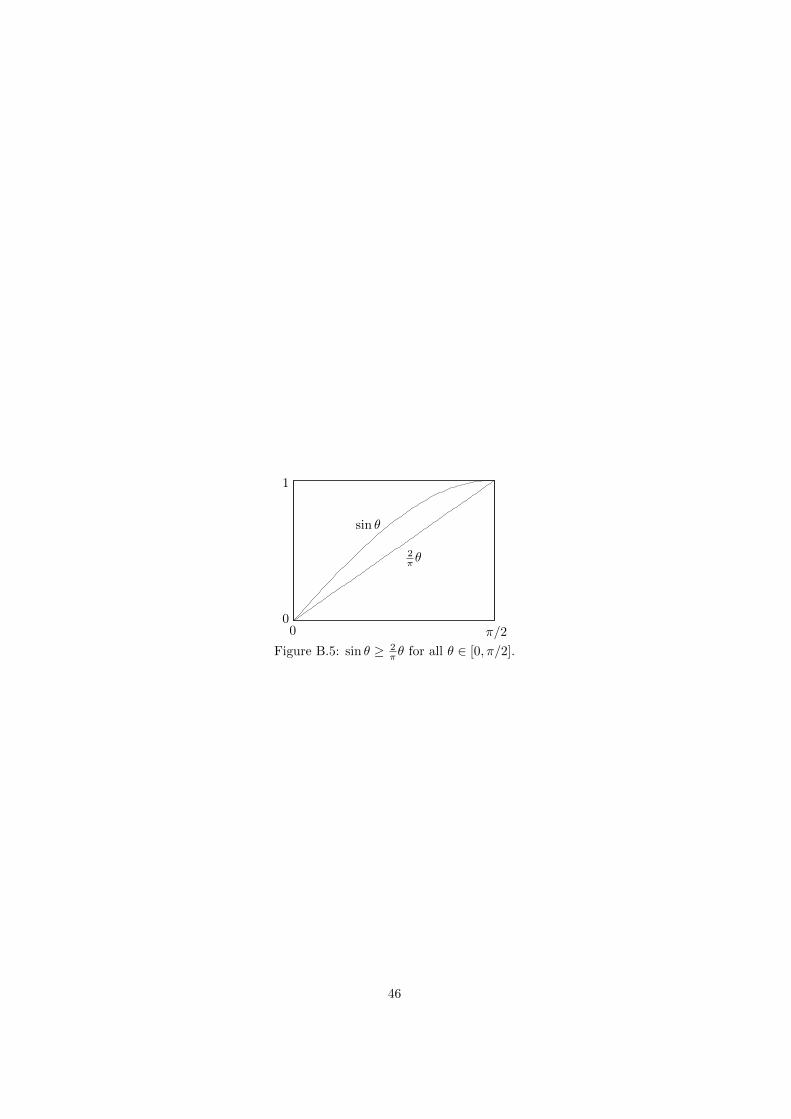
We use the fact that sin θ ≥ 2π θ for all θ ∈ [0, π/2]. (This can be proved using
convexity; see Figure B.5.) Now∫δ<|t|≤1/2
FN (t) dt =2
N + 1
∫ 1/2
δ
sin2((N + 1)πt)
sin2 πtdt (B:14)
≤ 2
N + 1
∫ 1/2
δ
1
(2t)2dt (B:15)
=1
2(N + 1)
(1
δ− 2)
(B:16)
→ 0 as N →∞. (B:17)
Here (B:14) follows from Lemma B7.2 and FN being even, (B:15) is becausesin2((n+ 1)πt) ≤ 1 and | sinπt| ≥ 2
π · πt, and (B:16) is a routine calculation. �
45
0 π/20
1
sin θ
2π θ
Figure B.5: sin θ ≥ 2π θ for all θ ∈ [0, π/2].
46
B8 The main theorem
For the lecture of Thursday 27 February 2014; part two of two
We can now prove the main theorem of Part B. It states that Fourier’s ideaworks perfectly when we use the 2- or 1-norm.
Theorem B8.1 Let f : T → C be an integrable function. Then Snf → f inboth ‖ · ‖2 and ‖ · ‖1.
Proof For all n, the Fejer kernel Fn is a trigonometric polynomial, so f ∗ Fnis a trigonometric polynomial (Lemma B3.4). Also, (Fn) is a PAD (Proposi-tion B7.3), so f ∗ Fn → f in ‖ · ‖2 (Proposition B5.5). Hence f is the limit in‖ · ‖2 of a sequence of trigonometric polynomials. So by Lemma B1.3, Snf → fin ‖ · ‖2. Finally, by Lemma A4.10, Snf → f in ‖ · ‖1. �
Corollary B8.2 The set {trigonometric polynomials} is dense in {integrablefunctions T→ C} with respect to both ‖ · ‖2 and ‖ · ‖1.
Proof This follows from Theorem B8.1, noting that the Fourier partial sumsSnf are trigonometric polynomials. �
In other words, if f is a point in the space of all integrable functions onT, then there are trigonometric polynomials arbitrarily close to f . (CompareProposition A9.4 on step functions.)
Theorem B8.3 (Parseval) Let f : T→ C be an integrable function. Then
‖f‖2 =
√√√√ ∞∑k=−∞
∣∣f(k)∣∣2.
Proof Snf → f in ‖·‖2, so ‖Snf‖2 → ‖f‖2 by Lemma A4.7, so ‖Snf‖22 → ‖f‖22.But
‖Snf‖22 =
n∑k=−n
∣∣f(k)∣∣2
by Lemma B1.1, so the result follows. �
In a suitable sense, Parseval’s theorem says that the map f 7→ f is anisometry (distance-preserving). It is also angle-preserving:
Corollary B8.4 Let f, g : T→ C be integrable functions. Then∫Tf(x)g(x) dx =
∞∑k=−∞
f(k)g(k).
Proof Sheet 3, q.5. �
Finally, the map f 7→ f is, essentially, injective:
47
Corollary B8.5 Let f, g : T→ C be integrable functions such that f(k) = g(k)for all k ∈ Z. Then:
i. f = g a.e.;
ii. f(x) = g(x) for all x ∈ T such that f and g are both continuous at x;
iii. f = g if f and g are both continuous.
Proof We have f − g(k) = 0 for all k ∈ Z (using Lemma A7.7(i)), so ‖f−g‖2 =0 by Parseval’s theorem. All three parts now follow from Lemma A4.5. �
This result does not mention the 2-norm (or indeed any norm) in its state-ment, although it does use the 2-norm in its proof. It answers a very fundamentalquestion about Fourier series, telling us:
Different functions have different Fourier series.
Here ‘different functions’ must be understood as ‘functions that are not almosteverywhere equal’, since it’s a basic fact that if f = g a.e. then f and g havethe same Fourier coefficients; see A3.13.
This encourages us to believe in Fantasy A8.7.
48
Chapter C
Uniform and pointwiseconvergence of Fourierseries
In Remark A4.11, we met this diagram:
‖ · ‖∞u} tttttt
#+NNNNNNNN
‖ · ‖2v~ uuuuuu
pointwise
"*LLLLLLLLLL
‖ · ‖1 a.e.
Part B covered the lower-left region of the diagram: convergence of Fourier seriesin the 2- and 1-norms. In Part C, we look at the upper-right region: uniformand pointwise convergence. (We will never look seriously at almost everywhereconvergence.)
C1 Warm-up
For the lecture of Monday 3 March 2014; part one of two
In Part B, we showed:
for all integrable f : T→ C, Snf → f in ‖ · ‖2 and ‖ · ‖1.
Is it also true in ‖ · ‖∞?No, since if Snf → f in ‖ · ‖∞ then f is continuous (by Fact A4.8), whereas
not every integrable function is continuous.But this leaves open the possibility that:
for all continuous f : T→ C, Snf → f in ‖ · ‖∞.
However, this is not true either. By du Bois–Reymond’s example (Theo-rem A2.2), there is some continuous f : T → C such that Snf does not evenconverge pointwise to f , let alone uniformly.
49
So if we’re hoping for all Fourier series to converge in either the uniform orpointwise sense, we’ll be disappointed. But perhaps it’s true if we dilute ourhopes, asking only for convergence almost everywhere. In other words, we mighthope that:
for all continuous f : T→ C, Snf → f almost everywhere.
This is true, by Carleson’s theorem (Theorem A2.6). But as previously men-tioned, all known proofs are much too hard for this course.
However, there are some easier results available. For example, we will beable to prove the theorem of Dirichlet that if f is continuously differentiable,then Snf → f uniformly (hence in all five senses). We will also look at anapplication that seems to have nothing to do with Fourier theory: the so-calledequidistribution theorem of Weyl, concerning the statistical behaviour of mul-tiples of irrational numbers.
We begin by collecting a few basic facts.As described in Fantasy A8.7, the theory of Fourier series is about the back-
and-forth between functions on T and doubly infinite sequences. So far, we haveconcentrated on the passage in one direction, starting with a function f on Tand deriving the double sequence (f(k))k∈Z. Let us now consider the oppositedirection. Write
CZ ={
double sequences c = (ck)∞k=−∞ in C}.
Lemma C1.1 Let c ∈ CZ. Then
∞∑k=−∞
|ck| <∞ ⇒∞∑
k=−∞
|ck|2 <∞ ⇒ supk∈Z|ck| <∞.
(This should remind you of the situation with convergence in the 1-, 2- and∞-norms—but it’s the other way round. Notice that squaring a small positivenumber decreases it.)
Proof For the first implication, suppose that∑∞k=−∞ |ck| <∞. Then certainly
the set {|ck| : k ∈ Z} is bounded; put ‖c‖∞ = supk∈Z |ck|. For all n ≥ 0, wehave
n∑k=−n
|ck|2 ≤ ‖c‖∞n∑
k=−n
|ck| ≤ ‖c‖∞∞∑
k=−∞
|ck|,
so∑∞k=−∞ |ck|2 <∞.
For the second implication, if∑∞k=−∞ |ck|2 < ∞ then {|ck|2 : k ∈ Z} is
bounded, so {|ck| : k ∈ Z} is bounded too. �
Remark C1.2 No further implications hold. To see that the converse of thefirst implication fails, consider
ck =
{1/k if k ≥ 1
0 if k ≤ 0.
To see that the converse of the second implication fails, take ck = 1 for all k.
50
Here is another basic fact. It is about convergence in the 1-norm, but willbe useful for arguments about uniform and pointwise convergence.
Lemma C1.3 Let c ∈ CZ and let f : T→ C be an integrable function. Supposethat
∑nk=−n ckek → f in ‖ · ‖1 as n→∞. Then ck = f(k) for all k ∈ Z.
Proof For each n ≥ 0, write gn =∑nk=−n ckek. Let ` ∈ Z. By Lemma A7.7(ii),
gn(`) → f(`) as n → ∞. But by Lemma A8.3, gn(`) = c` whenever n ≥ |`|, so
c` = f(`), as required. �
We can now answer a subtle question that has been present from the begin-ning. Can it happen that the Fourier series of f converges, but not to f? Forconvergence in the uniform sense, no.
Lemma C1.4 Let f : T → C be an integrable function. Suppose that the se-quence (Snf)∞n=0 converges uniformly (not necessarily to f). Then:
i. (Snf)(x)→ f(x) for almost all x ∈ T;
ii. (Snf)(x)→ f(x) for all x ∈ T such that f is continuous at x;
iii. Snf → f uniformly if f is continuous.
Part (iii) says that for a continuous function f , if Snf converges uniformlyto something, that something must be f .
Proof Let g be the uniform limit of the sequence (Snf). By Fact A4.8, g is
continuous. Certainly Snf → g in ‖ · ‖1, so f(k) = g(k) for all k ∈ Z by
Lemma C1.3 (taking ‘ck’ to be f(k) and ‘f ’ to be g). The result now followsfrom Corollary B8.5. �
51
C2 What if the Fourier coefficients are abso-lutely summable?
For the lecture of Monday 3 March 2014; part two of two
We saw in Proposition B1.2 that∑∞k=−∞ |f(k)|2 < ∞ for any integrable func-
tion f : T → C. However, f may or may not have the stronger property that∑∞k=−∞ |f(k)| <∞. (To see why this is stronger, recall Lemma C1.1.)
In this section, we will see that if∑∞k=−∞ |f(k)| <∞ then the Fourier series
of f behaves well, in a sense that will be made precise. In the next section, wewill see that many common functions do have this property.
We begin with a result on double sequences.
Proposition C2.1 Let c ∈ CZ. Suppose that∑∞k=−∞ |ck| < ∞. Then the
sequence(∑n
k=−n ckek
)∞n=0
converges uniformly to a continuous function g.
Moreover, g(k) = ck for all k ∈ Z.
Proof For n ≥ 0, write sn =∑nk=−n ckek.
First we show that the sequence (sn) converges pointwise. Indeed, let x ∈ T.Given ε > 0, we can choose N such that
∑k : |k|≥N |ck| < ε; then for all m ≥
n ≥ N ,
|sm(x)− sn(x)| =
∣∣∣∣∣ ∑k : n<|k|≤m
ckek(x)
∣∣∣∣∣ ≤ ∑k : n<|k|≤m
|ck| < ε.
So the sequence (sn(x))∞n=0 is Cauchy, and therefore convergent, as claimed.Next, for each x ∈ T, put
g(x) = limn→∞
sn(x) =
∞∑k=−∞
ckek(x).
This defines a function g : T→ C. Now (sn) converges uniformly to g, since
‖sn − g‖∞ = supx∈T
∣∣∣∣∣ ∑k : |k|>n
ckek(x)
∣∣∣∣∣ ≤ ∑k : |k|>n
|ck| → 0
as n → ∞. By Fact A4.8, g is therefore continuous, and by Lemma C1.3,g(k) = ck for all k ∈ Z. �
We now come to the most important result of Part C so far.
Theorem C2.2 Let f : T → C be an integrable function. Suppose that∑∞k=−∞ |f(k)| <∞. Then:
i. (Snf)(x)→ f(x) as n→∞ for all x ∈ T such that f is continuous at x;
ii. Snf → f uniformly if f is continuous.
Proof By Proposition C2.1 (taking ck to be f(k)), the Fourier partial sums Snf
converge uniformly to some continuous function g : T→ C, and g(k) = f(k) forall k ∈ Z. The result follows from Corollary B8.5. �
52
C3 Continuously differentiable functions
For the lecture of Thursday 6 March 2014; part one of two
We have just shown that if∑∞k=−∞ |f(k)| < ∞ then the Fourier series of
f behaves well (Theorem C2.2). If you had a particular function f in front ofyou, you might be able to calculate its Fourier coefficients, you might be ableto calculate the sum of their absolute values, and that sum might be finite.In that case, you could conclude that the Fourier series of that particular fwas well-behaved. But are there general conditions on f guaranteeing that∑∞k=−∞ |f(k)| <∞?The answer turns out to be yes. But beware that not all integrable functions
f : T → C satisfy∑|f(k)| < ∞. In fact, there exist quite ‘nice’ functions f
with∑|f(k)| =∞:
Example C3.1 Define f : T→ C by
f(x) =∑n≥2
sin(2πnx)
n log n.
One can show that Snf → f uniformly, and so f is continuous. One can alsoshow that
∑|f(k)| = ∞. (The proof of both these statements is omitted and
non-examinable.) So a continuous function f need not satisfy∑|f(k)| <∞.
However, we will see that if f is smooth enough, the Fourier coefficientsdecay fast enough that
∑|f(k)| converges.
Definition C3.2 Let n ≥ 0. We write Cn(T) for the set of functions T → Cwhose corresponding 1-periodic function g : R → C is n times continuouslydifferentiable (that is, g(n) exists and is continuous). We also write
C(T) = C0(T) = {continuous functions T→ C}.
For example, a function T → C belongs to the set C1(T) if and only if thecorresponding 1-periodic function R→ C is continuously differentiable.
Lemma C3.3 Let n ≥ 0, f ∈ Cn(T), and k ∈ Z. Then
f (n)(k) = (2πik)nf(k).
Proof Sheet 3, q.6(ii). �
In other words, differentiating f amounts to multiplying its kth Fouriercoefficient by 2πik.
We can now prove the 1829 theorem of Dirichlet, one of the early landmarksof Fourier analysis. In fact, what we prove is stronger than the version statedearlier (Theorem A2.1): there, we only asserted pointwise convergence, but herewe prove uniform convergence.
Theorem C3.4 (Dirichlet) Let f ∈ C1(T). Then∑∞k=−∞ |f(k)| < ∞ and
Snf → f uniformly.
53
Since uniform convergence is the strongest kind of convergence, this tells usthat the Fourier series of a continuously differentiable function converges in allfive senses. Thus, it behaves as well as any function could.
Proof For k 6= 0, we have
|f(k)| = |f ′(k)| · 1
2π|k|(C:1)
≤ 1
2
(|f ′(k)|2 +
1
(2π|k|)2
)(C:2)
=|f ′(k)|2
2+
1
8π2k2, (C:3)
where in (C:1) we used Lemma C3.3 and in (C:2) we used the fact that uv ≤12 (u2 + v2) for all u, v ∈ R (proof: exercise). So to show that
∑∞k=−∞ |f(k)| is
finite, it suffices to show that the sum of (C:3) over all k ∈ Z is finite. First, f ′ is
continuous and so integrable; hence∑∞k=−∞ |f ′(k)|2 <∞ by Proposition B1.2.
Second, ∑06=k∈Z
1
k2= 2
∑k≥1
1
k2<∞.
Hence∑∞k=−∞ |f(k)| <∞, giving Snf → f uniformly by Theorem C2.2. �
Remark C3.5 We have just shown that
f ∈ C1(T) ⇒∑|f(k)| <∞.
But the converse fails, even for continuous functions. Here is an example dueto Weierstrass:
f(x) =
∞∑n=1
2−n cos(2nπx).
It can be shown (non-examinably) that∑|f(k)| < ∞ and that f is continu-
ous. But it can also be shown that f is not differentiable anywhere, let alonecontinuously differentiable everywhere.
54
C4 Fejer’s theorem
For the lecture of Thursday 6 March 2014; part two of two
Du Bois–Reymond’s example (Theorem A2.2) tells us that for a continuousfunction f : T → C and a point x ∈ T, the sequence
((Snf)(x)
)∞n=0
need nothave a limit. However, Fejer showed that it always has a Cesaro limit, namely,f(x). His result is the centrepiece of this section.
In Part B, we proved that Snf → f in ‖ · ‖2 by proving that f ∗ Fn → f in‖ · ‖2. We did that by proving that (i) (Fn) is a PAD, and (ii) f ∗Kn → f in‖ · ‖2 for any PAD (Kn). We adopt a similar strategy here, but with pointwiseand uniform convergence in place of mean square convergence.
For integrable f : T→ C, we have
f ∗ Fn = f ∗ 1
n+ 1(D0 + · · ·+Dn)
=1
n+ 1(f ∗D0 + · · ·+ f ∗Dn)
=1
n+ 1(S0f + · · ·+ Snf).
This is nothing but the nth Cesaro mean of the sequence S0f, S1f, . . .. We willwrite
Anf =1
n+ 1(S0f + · · ·+ Snf) = f ∗ Fn.
To say that f(x) is the Cesaro limit of the sequence ((Snf)(x)) is to say that(Anf)(x)→ f(x) as n→∞, or equivalently that (f ∗Fn)(x)→ f(x) as n→∞.
Here is a summary of the notation and terminology:
Ordinary convergence Cesaro convergencenth term in sequence Snf Anfnth kernel Dn (Dirichlet) Fn (Fejer)
To prove Fejer’s theorem, we will need to know a little more about PADs.We showed in Section B5 that for any PAD (Kn) and integrable function f , wehave f ∗Kn → f in both ‖ · ‖2 and ‖ · ‖1. That result cannot be strengthenedto convergence in ‖ · ‖∞ for arbitrary integrable functions f , since each f ∗Kn
is continuous and a uniform limit of continuous functions is continuous. So thebest we could hope for is that if f is continuous then f ∗ Kn → f in ‖ · ‖∞.We might also hope to be able to prove a result about convergence at particularpoints. Both these hopes are fulfilled:
Proposition C4.1 Let (Kn) be a PAD and f : T → C an integrable function.Then:
i. (f ∗Kn)(x)→ f(x) as n→∞ for all x ∈ T such that f is continuous atx;
ii. f ∗Kn → f uniformly if f is continuous.
The proof is similar to the proof of Proposition B5.4, the correspondingresult for the 1-norm.
55
Proof For (i), let x ∈ T. In the proof of Proposition B5.4, equation (B:7)stated that for all n ≥ 0 and δ ∈ (0, 1/2),
|(f ∗Kn)(x)−f(x)| ≤∫|t|<δ
|f(x−t)−f(x)|Kn(t) dt+2‖f‖∞∫δ<|t|≤1/2
Kn(t) dt.
Suppose that f is continuous at x. Let ε > 0. Choose δ ∈ (0, 1/2) such that|f(x− t)− f(x)| < ε/2 for all t ∈ (−δ, δ). By PAD3, we can also choose N suchthat for all n ≥ N , ∫
δ<|t|≤1/2
Kn(t) dt <ε
4‖f‖∞.
Then for all n ≥ N ,
|(f ∗Kn)(x)− f(x)| ≤ ε
2
∫|t|<δ
Kn(t) dt+ 2‖f‖∞ ·ε
4‖f‖∞
≤ ε
2
∫ 1/2
−1/2
Kn(t) dt+ε
2= ε,
as required.For (ii), suppose that f is continuous. Let ε > 0. Every continuous map
from a compact metric space to a metric space is uniformly continuous, and Tis compact, so f is uniformly continuous. Hence we can choose δ ∈ (0, 1/2) suchthat for all x ∈ T and t ∈ (−δ, δ), we have |f(x− t)− f(x)| < ε/2.
(In case you have not previously encountered this theorem about metricspaces, an alternative argument is available. Here we use instead the theoremthat any continuous function on a closed bounded interval is uniformly contin-uous. Since f is continuous on [−1, 1], it is uniformly continuous there. So byinterpreting T as [−1/2, 1/2), we can choose δ as in the last paragraph.)
By PAD3, we can choose N as in the proof of (i). For all x ∈ T, for alln ≥ N , we calculate that |(f ∗Kn)(x)− f(x)| < ε, again as in the proof of (i).So ‖f ∗Kn − f‖∞ ≤ ε for all n ≥ N , as required. �
Theorem C4.2 (Fejer) Let f : T→ C be an integrable function. Then:
i. (Anf)(x)→ f(x) as n→∞ for all x ∈ T such that f is continuous at x;
ii. Anf → f uniformly if f is continuous.
Proof (Fn) is a PAD and Anf = f ∗ Fn, so this follows from the last proposi-tion. �
Looking back at du Bois–Reymond’s example (Theorem A2.2), we see thatthe sequence (Anf) is more likely to converge than the sequence (Snf).
Remark C4.3 If f, g : T→ C with f(k) = g(k) for all k, then Anf = Ang forall n, so by Fejer’s theorem, f(x) = g(x) for all x ∈ T such that f and g are bothcontinuous at x. This gives an alternative proof of Corollary B8.5(ii), (iii). Butunlike that corollary, Fejer’s theorem gives an explicit way of reconstructingf from its Fourier coefficients (at least for continuous f): from knowing theFourier coefficients, we can compute Anf for each n, and we then obtain f(x)as limn→∞(Anf)(x).
56
Corollary C4.4 The set {trigonometric polynomials} is dense in C(T) withrespect to ‖ · ‖∞.
Proof Let f ∈ C(T). For each n ≥ 0, the function Anf is a trigonometricpolynomial, since S0f, . . . , Snf are. The result follows from part (ii) of Fejer’stheorem. �
By Lemma A4.10(i), density with respect to ‖ · ‖∞ is the strongest type ofdensity (that is, stronger than density with respect to ‖ · ‖2 or ‖ · ‖1). Corol-lary C4.4 can be compared to Corollary B8.2, which stated that the set oftrigonometric polynomials is dense in the set of integrable functions with re-spect to ‖ · ‖2 (hence ‖ · ‖1).
(Faced with this, it is natural to ask whether Corollary B8.2 can be improvedto density with respect to ‖ · ‖∞. The answer is no, again because a uniformlimit of continuous functions is continuous.)
Corollary C4.5 (Weierstrass approximation theorem) Let I ⊆ R be aclosed bounded interval and f : I → C a continuous function. Then for allε > 0, there exists a polynomial p over C such that supx∈I |f(x)− p(x)| ≤ ε.
Proof Sheet 4. �
This result is important in many ways. For example, it is a basic fact innumerical analysis, where we might wish to approximate an arbitrary continuousfunction by a polynomial. However, we will not need it for anything in the restof this course.
57
C5 Differentiable functions and the Riemann lo-calization principle
For the lecture of Monday 10 March
This section contains two major results. First, there is a convergence theoremfor differentiable functions, to add to our existing convergence theorem for con-tinuously differentiable functions (Dirichlet’s Theorem C3.4). Then, we meetthe deep and shocking ‘localization principle’ of Riemann.
Dirichlet’s theorem states that if f is continuously differentiable then Snf →f uniformly. We will weaken both the hypothesis and the conclusion, provingthat if f is differentiable (but not necessarily continuously so) then Snf → fpointwise (but not necessarily uniformly).
To prove this, we need another fact about integration.
Fact C5.1 Let I ⊆ R be a bounded interval and x ∈ I. Let g : I → C be abounded function such that for all δ > 0, the restriction g|I\(x−δ,x+δ) is inte-grable. Then g is integrable.
The proof is omitted and non-examinable, but can be found in the appendixof the book Fourier Analysis by Stein and Shakarchi.
Theorem C5.2 Let f : T→ C be an integrable function. Then:
i. (Snf)(x)→ f(x) for all x ∈ T such that f is differentiable at x;
ii. Snf → f pointwise if f is differentiable.
Proof We just have to prove (i), since this immediately implies (ii). Take x ∈ Tsuch that f is differentiable at x.
For all n ≥ 0,
f(x)− (Snf)(x) =
∫TDn(t)f(x) dt−
∫TDn(t)f(x− t) dt (C:4)
=
∫T
en+1(t)− e−n(t)
e1(t)− 1(f(x)− f(x− t)) dt (C:5)
=
∫T(en+1(t)− e−n(t))g(t) dt, (C:6)
where in (C:4) we used the fact that∫TDn(t) dt = 1, in (C:5) we used equa-
tion (B:13) (from the proof of Lemma B7.2), and in (C:6) we put
g(t) =f(x)− f(x− t)
e1(t)− 1
for 0 < |t| ≤ 1/2. If g is integrable then
f(x)− (Snf)(x) = g(−(n+ 1))− g(n)→ 0− 0 = 0
as n → ∞, by the Riemann–Lebesgue lemma (Proposition B1.2), completingthe proof. So it is enough to prove that g is integrable. To do this, we will needthe assumption that f is differentiable at x, which we have not used yet.
58
We prove that g is integrable using Fact C5.1.First we show that for each δ > 0, the function g|[−1/2,1/2)\(−δ,δ) is integrable.
Let δ > 0. By Lemma A3.7, it is enough to show that the restrictions of thefunctions
t 7→ 1/(e1(t)− 1), t 7→ f(x)− f(x− t)
to [−1/2, 1/2) \ (−δ, δ) are both integrable. And indeed, the first restrictedfunction is integrable because it is continuous and bounded, and the second isintegrable because f is.
Next we show that g is bounded. For 0 < |t| ≤ 1/2, we have
g(t) =f(x)− f(x− t)
t· t
e1(t)− 1→ f ′(x) · 1
2πias t→ 0,
using l’Hopital’s rule in the second factor. Define g(0) = f ′(x)/2πi; then g iscontinuous at 0, so there exists η > 0 such that g|(−η,η) is bounded. But also,g|[−1/2,1/2)\(−η,η) is bounded (since it is integrable). Hence g itself is bounded.
It follows from Fact C5.1 that g is integrable, as required. �
It once seems to have been believed that although a continuous functionneed not be differentiable everywhere, it must be differentiable somewhere. Ifthis were the case, Theorem C5.2 would tell us that the Fourier series of acontinuous function f must converge to f(x) for at least one value of x. However,Weierstrass’s example of a continuous function that is nowhere differentiable(Remark C3.5) shows that this strategy will not work.
We now use Theorem C5.2 to deduce the second major result of this sec-tion, the Riemann localization principle. A good way to prepare for this is tolook back at Section A1 (the algebraist’s dream), and especially the two pointslabelled ‘7’ there.
Remark C5.3 The Taylor series
(Tf)(x) =
∞∑n=0
f (n)(0)
n!xn
of an infinitely differentiable function f is ‘determined locally’ at 0. That is, iff, g : R→ C with f |(−δ,δ) = g|(−δ,δ) for some δ > 0, then Tf = Tg. In contrast,the Fourier series of f : C→ C is not determined locally at 0 (or indeed at anyother point), since each coefficient
f(k) =
∫Tf(t)e−2πikt dt
involves all of f . Thus, given f, g : T → C with f |(−δ,δ) = g|(−δ,δ) for someδ > 0, we can not deduce that Sf = Sg.
The next result therefore comes as a surprise.
Corollary C5.4 (Riemann localization principle) Let f, g : T → C be in-tegrable functions and x ∈ T. Suppose there exists δ > 0 such that f |(x−δ,x+δ) =g|(x−δ,x+δ). Then
(Snf)(x)→ f(x) as n→∞ ⇐⇒ (Sng)(x)→ g(x) as n→∞.
59
In other words, whether or not the Fourier series of f at x converges to f(x)depends only on the behaviour of f near x.
Proof The integrable function f − g : T → C has constant value 0 on someneighbourhood of x, so is differentiable at x. Hence by Theorem C5.2,
(Sn(f − g))(x)→ (f − g)(x) as n→∞.
Equivalently,(Snf)(x)− (Sng)(x)→ 0 as n→∞.
The result follows. �
The theme of ‘local versus global’ becomes increasingly visible at this levelof mathematics. You may have met it in differential geometry; for example,a surface is locally like R2, but globally may be quite unlike it. In numbertheory, there is the local-to-global principle of Hasse, which has to do with p-adicnumbers and is helpful in determining the solvability of polynomial equationsover the integers. The interplay between local and global is captured formallyby the notion of sheaf, which is especially prominent in algebraic geometry.
60
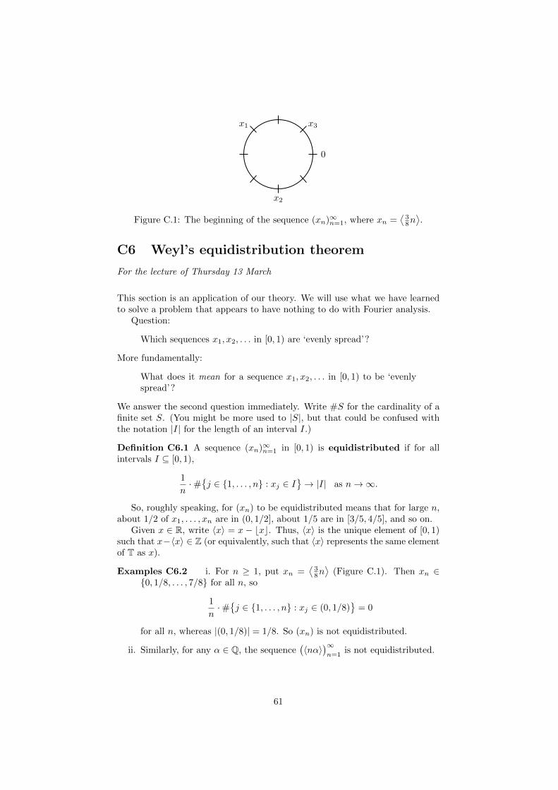
0
x1
x2
x3
Figure C.1: The beginning of the sequence (xn)∞n=1, where xn =⟨
38n⟩.
C6 Weyl’s equidistribution theorem
For the lecture of Thursday 13 March
This section is an application of our theory. We will use what we have learnedto solve a problem that appears to have nothing to do with Fourier analysis.
Question:
Which sequences x1, x2, . . . in [0, 1) are ‘evenly spread’?
More fundamentally:
What does it mean for a sequence x1, x2, . . . in [0, 1) to be ‘evenlyspread’?
We answer the second question immediately. Write #S for the cardinality of afinite set S. (You might be more used to |S|, but that could be confused withthe notation |I| for the length of an interval I.)
Definition C6.1 A sequence (xn)∞n=1 in [0, 1) is equidistributed if for allintervals I ⊆ [0, 1),
1
n·#{j ∈ {1, . . . , n} : xj ∈ I
}→ |I| as n→∞.
So, roughly speaking, for (xn) to be equidistributed means that for large n,about 1/2 of x1, . . . , xn are in (0, 1/2], about 1/5 are in [3/5, 4/5], and so on.
Given x ∈ R, write 〈x〉 = x− bxc. Thus, 〈x〉 is the unique element of [0, 1)such that x−〈x〉 ∈ Z (or equivalently, such that 〈x〉 represents the same elementof T as x).
Examples C6.2 i. For n ≥ 1, put xn =⟨
38n⟩
(Figure C.1). Then xn ∈{0, 1/8, . . . , 7/8} for all n, so
1
n·#{j ∈ {1, . . . , n} : xj ∈ (0, 1/8)
}= 0
for all n, whereas |(0, 1/8)| = 1/8. So (xn) is not equidistributed.
ii. Similarly, for any α ∈ Q, the sequence(〈nα〉
)∞n=1
is not equidistributed.
61
So far, we haven’t seen any examples of equidistributed sequences, only non-examples. It’s not obvious that there are any equidistributed sequences at all!But using Fourier analysis, we’ll construct lots.
When we defined equidistributed sequence, we were choosing a precise mean-ing for the phrase ‘evenly spread’. But here’s a different, less obvious interpre-tation. We could say that a sequence (xn) in [0, 1) is ‘evenly spread’ if for allintegrable functions f : T→ C,
1
n
n∑j=1
f(xj)→∫ 1
0
f(t) dt as n→∞. (C:7)
Think for a while about why this is a sensible idea—understanding the rest ofthis section depends on it.
There are variations on this idea in which we use different classes of func-tions. For instance, we could regard (xn) as ‘evenly spread’ if (C:7) holds forall continuous (rather than integrable) functions f , or all step functions, or allcharacters, etc. Actually, one of these variations produces the notion of equidis-tributed sequence itself:
Lemma C6.3 Let (xn)∞n=1 be a sequence in [0, 1). Then (xn) is equidistributedif and only if (C:7) holds whenever f is the characteristic function of an intervalin [0, 1).
Proof For an interval I ⊆ [0, 1), and for n ≥ 1, we have
1
n
n∑j=1
χI(xj) =1
n#{j ∈ {1, . . . , n} : xj ∈ I
}and ∫ 1
0
χI(t) dt = |I| .
The result follows. �
We now show that all these notions of ‘evenly spread’ sequence produced bychoosing different classes of function are, in fact, the same.
Theorem C6.4 Let (xn)∞n=1 be a sequence in [0, 1). The following are equiva-lent:
i. (C:7) holds for all integrable f : T→ C;
ii. (C:7) holds for all characters f = ek : T→ C, where k ∈ Z;
iii. (C:7) holds for all trigonometric polynomials f : T→ C;
iv. (C:7) holds for all continuous f : T→ C;
v. (C:7) holds for all characteristic functions f = χI : T → C, where I ⊆[0, 1) is an interval;
vi. (C:7) holds for all step functions f : T→ C.
62
Proof We show that (i) ⇒ (ii) ⇒ (iii) ⇒ (iv) ⇒ (v) ⇒ (vi) ⇒ (i).(i) ⇒ (ii): trivial.(ii)⇒ (iii): assume (ii). Let f =
∑mk=−m ckek be a trigonometric polynomial.
Then
1
n
m∑j=1
f(xj) =
m∑k=−m
ck ·1
n
n∑j=1
ek(xj)→m∑
k=−m
ck
∫ 1
0
ek(t) dt =
∫ 1
0
f(t) dt
as n→∞.(iii) ⇒ (iv): assume (iii). Let f : T → C be a continuous function. Let
ε > 0. By Corollary C4.4, we can find a trigonometric polynomial g such that‖f − g‖∞ < ε/3. By assumption, we can choose N such that for all n ≥ N ,∣∣∣∣ 1n
n∑j=1
g(xj)−∫ 1
0
g(t) dt
∣∣∣∣ < ε/3.
Then for all n ≥ N , using the triangle inequality,∣∣∣∣ 1nn∑j=1
f(xj)−∫ 1
0
f(t) dt
∣∣∣∣ ≤ ∣∣∣∣ 1nn∑j=1
f(xj)−1
n
n∑j=1
g(xj)
∣∣∣∣+
∣∣∣∣ 1nn∑j=1
g(xj)−∫ 1
0
g(t) dt
∣∣∣∣+
∣∣∣∣∫ 1
0
g(t) dt−∫ 1
0
f(t) dt
∣∣∣∣<
1
n
n∑j=1
‖f − g‖∞ + ε/3 + ‖f − g‖1
≤ ‖f − g‖∞ + ε/3 + ‖f − g‖∞ < ε.
(iv) ⇒ (v): assume (iv). Let I ⊆ [0, 1) be an interval, and let ε > 0. Wecan find a continuous function gU : [0, 1) → R such that gU (t) ≥ χI(t) for allt ∈ [0, 1) and ∫ 1
0
gU (t) dt−∫ 1
0
χI(t) dt < ε/2
(Figure C.2). By assumption, we can choose N ≥ 1 such that for all n ≥ N ,∣∣∣∣ 1nn∑j=1
gU (xj)−∫ 1
0
gU (t) dt
∣∣∣∣ < ε/2.
So for all n ≥ N ,
1
n
n∑j=1
χI(xj)−∫ 1
0
χI(t) dt (C:8)
≤ 1
n
n∑j=1
gU (xj)−∫ 1
0
χI(t) dt
=
(1
n
n∑j=1
gU (xj)−∫ 1
0
gU (t) dt
)+
(∫ 1
0
gU (t) dt−∫ 1
0
χI(t) dt
)< ε/2 + ε/2 = ε.
63
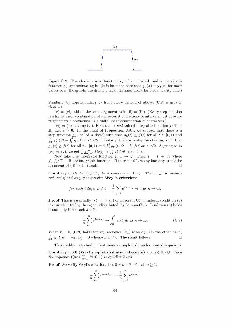
χI
gU
Figure C.2: The characteristic function χI of an interval, and a continuousfunction gU approximating it. (It is intended here that gU (x) = χI(x) for mostvalues of x; the graphs are drawn a small distance apart for visual clarity only.)
Similarly, by approximating χI from below instead of above, (C:8) is greaterthan −ε.
(v)⇒ (vi): this is the same argument as in (ii)⇒ (iii). (Every step functionis a finite linear combination of characteristic functions of intervals, just as everytrigonometric polynomial is a finite linear combination of characters.)
(vi) ⇒ (i): assume (vi). First take a real -valued integrable function f : T→R. Let ε > 0. In the proof of Proposition A9.4, we showed that there is astep function gL (called g there) such that gL(t) ≤ f(t) for all t ∈ [0, 1) and∫ 1
0f(t) dt −
∫ 1
0gL(t) dt < ε/2. Similarly, there is a step function gU such that
gU (t) ≥ f(t) for all t ∈ [0, 1) and∫ 1
0gU (t) dt −
∫ 1
0f(t) dt < ε/2. Arguing as in
(iv) ⇒ (v), we get 1n
∑nj=1 f(xj)→
∫ 1
0f(t) dt as n→∞.
Now take any integrable function f : T → C. Then f = f1 + if2 wheref1, f2 : T→ R are integrable functions. The result follows by linearity, using theargument of (ii) ⇒ (iii) again. �
Corollary C6.5 Let (xn)∞n=1 be a sequence in [0, 1). Then (xn) is equidis-tributed if and only if it satisfies Weyl’s criterion:
for each integer k 6= 0,1
n
n∑j=1
e2πikxj → 0 as n→∞.
Proof This is essentially (v) ⇐⇒ (ii) of Theorem C6.4. Indeed, condition (v)is equivalent to (xn) being equidistributed, by Lemma C6.3. Condition (ii) holdsif and only if for each k ∈ Z,
1
n
n∑j=1
e2πikxj →∫ 1
0
ek(t) dt as n→∞. (C:9)
When k = 0, (C:9) holds for any sequence (xn) (check!). On the other hand,∫ 1
0ek(t) dt = 〈ek, e0〉 = 0 whenever k 6= 0. The result follows. �
This enables us to find, at last, some examples of equidistributed sequences.
Corollary C6.6 (Weyl’s equidistribution theorem) Let α ∈ R \Q. Thenthe sequence
(〈nα〉
)∞n=1
in [0, 1) is equidistributed.
Proof We verify Weyl’s criterion. Let 0 6= k ∈ Z. For all n ≥ 1,
1
n
n∑j=1
e2πik〈jα〉 =1
n
n∑j=1
e2πikjα
64
since 〈jα〉 − jα ∈ Z. We sum this geometric series using the standard formula,which is valid as long as the ratio is not equal to 1. Here, this means e2πikα 6= 1,or equivalently kα 6∈ Z, which is true as k 6= 0 and α 6∈ Q. Thus, the formula isvalid and the sum of the geometric series is
1
ne2πikα e
2πiknα − 1
e2πikα − 1.
So for all n ≥ 1,∣∣∣∣ 1nn∑j=1
e2πik〈jα〉∣∣∣∣ ≤ 1
n·∣∣e2πiknα
∣∣+ |1|∣∣e2πikα − 1∣∣ =
1
n· 2∣∣e2πikα − 1
∣∣ → 0
as n→∞. �
Example C6.7 Consider the sequence
e = 2.718 . . . , 2e = 5.436 . . . , 3e = 8.154 . . . , . . . .
The sequence(〈ne〉
)∞n=1
of fractional parts is
0.718 . . . , 0.436 . . . , 0.154 . . . , . . . .
Weyl’s equidistribution theorem tells us that ‘in the long run’, about 1/100 ofthese fractional parts lie between 0.12 and 0.13 (for instance). In particular,there are infinitely many natural numbers n such that
0.12 ≤ 〈ne〉 < 0.13.
Could you prove this without Weyl’s theorem? Could you prove that there iseven one number n with this property?
65
Chapter D
Duality
This course is called Fourier Analysis, but we have focused throughout onFourier series. You’re aware that Fourier transforms are also important. Whatis the relationship between the two?
Section D1 gives the answer. We’ll see there that by looking at Fourieranalysis from sufficiently high altitude—by taking a bird’s eye view—it becomesapparent that Fourier series and Fourier transforms are two special cases of thesame general construction.
But it also becomes apparent that there are other interesting special cases.One case that is both interesting and easy is Fourier analysis on finite abeliangroups. That’s what we’ll study for the rest of Part D.
D1 An abstract view of Fourier analysis
For the lecture of Monday 17 March
This section (D1) is not directly examinable, but reading it is recommended: itshould help you to understand the ideas behind Part D and how it relates to therest of the course.
The right general context for Fourier analysis is that of topological groups. Tounderstand what a topological group is, you first need to know roughly whata topological space is. So here is a short, informal introduction to topologicalspaces.
Roughly speaking, a set X is called a topological space if we know whatit means to ‘move gradually’ within X. For instance, Rn is a topological spacebecause we know what it means for one point to be close to another, and weknow what a ‘continuous path’ in Rn is (namely, a continuous map [0, 1]→ Rn).Similarly, the sphere is a topological space: you know what it means to movegradually on the surface of the earth. The circle T is a topological space for thesame reason.
Some non-mathematical examples to help your intuition: the set of allcolours is a topological space, because you know what it means for a colourto change gradually. The set of all possible human faces is a topological space,because you know what it means for a face to change gradually (e.g. as you
66
age) or for one face to be similar to another. Your own changing face defines acontinuous map f from [0, 1] to the space of all faces, with f(0) being your faceat birth and f(1) your face at death.
Formally, a topological space is a set X equipped with some extra data(specifying what it means to ‘move gradually’). That extra data is called a‘topology’ on X. We will not need the formal definition.
Some topological spaces are rather trivial. For instance, you can’t movegradually from one integer to another without passing through non-integers, sothe set Z is a topological space in a trivial way: the only way of moving graduallyis to stay still. Formally, this is called the discrete topology on Z. (If you knowthe definition of topological space, the discrete topology is the topology in whichall subsets are open.) Any set can be given the discrete topology.
Topological spaces are the right context for the definition of continuous map.You know what continuity means for a function R→ R, and more generally fora function Rn → Rm, and also for a function T→ C. Given topological spacesX and Y , there is a definition of what it means for a function X → Y to becontinuous. The definitions for Rn, T, C, etc. are all special cases of this generaldefinition.
Roughly speaking, a topological group is a topological space that is alsoa group. We are most interested in those topological groups that are abelian(that is, the multiplication is commutative) and ‘locally compact’ (a conditionthat I will not explain; it is satisfied by all the examples I will mention). So,what we are interested in is locally compact, abelian topological groups, whichare usually just called ‘locally compact abelian groups’ or LCAGs for short.
Examples D1.1 i. Rn is a LCAG (with addition as the group operation),for any n ≥ 0.
ii. The circle T is a LCAG too. Recall that T is the quotient group R/Z, sothat its group operation is addition too.
iii. Z is a LCAG, with + as the group operation and the discrete topology.
iv. Any finite abelian group is a LCAG, with the discrete topology.
v. S = {z ∈ C : |z| = 1} is a LCAG, with · as the group operation. In fact,T ∼= S, via the map t 7→ e2πit.
Definition D1.2 Let G be a LCAG. A character of G is a continuous grouphomomorphism G→ S.
Examples D1.3 i. For each ξ ∈ Rn, there is a character eξ of Rn definedby
eξ(x) = e2πiξ.x
(x ∈ Rn), where ξ.x is the dot product of ξ and x. (This is the ordinaryproduct in the case n = 1.) You know that eξ is continuous, and you caneasily check that eξ is a group homomorphism (try it!). Fact: these arethe only characters of Rn.
ii. For each k ∈ Z, there is a character ek of T defined in the usual way.Lemma A7.2 states exactly that each ek is a character in the sense of Def-inition D1.2. Fact: these are the only characters of T. So, the charactersof T in our new sense are precisely the characters of T in our old sense.
67

iii. For each t ∈ T, there is a character εt of Z defined by
εt(k) = e2πikt
(t ∈ T). Again, you can easily check that each εt really is a character,that is, a continuous homomorphism. Fact: these are the only charactersof Z.
The setG = {characters of G}
forms a LCAG in a natural way. I won’t describe the topology, but the groupstructure is given ‘pointwise’: if e1 and e2 are characters of G then the charactere1 · e2 is defined by (e1 · e2)(x) = e1(x) · e2(x) (x ∈ G). The hat notation is
related to, but different from, the hat notation f for the Fourier coefficients orFourier transform of a function f .
Examples D1.3 tell us what G is for various LCAGs G:
G GRn RnT ZZ T
For instance, T ∼= Z because we have an isomorphism
Z → Tk 7→ ek.
We saw in Lemma A7.3 that this map is a homomorphism, and in Exam-ple D1.3(ii) that this map is surjective. It is not hard to see that it is alsoinjective (that is, ek and e` are different if k 6= `). So, it is an isomorphism ofgroups, and in fact an isomorphism of topological groups (that is, a homeomor-phism too).
In each of the three cases in the table,G ∼= G. In fact, this is a general
phenomenon:
Theorem D1.4 (Pontryagin duality)G ∼= G for all LCAGs G.
The group G can be thought of as the ‘mirror image’ of the group G (Fig-ure D.1). Pontryagin duality states that the mirror image of the mirror imageof G is G itself.
We now look briefly at Fourier analysis on locally compact abelian groups.Let G be a LCAG. ‘Nice’ functions on G can be integrated. For example,
you’re used to integrating nice functions on Rn or T. In the case of Z, a functionZ→ C is just a double sequence (ck)∞k=−∞ in C, and integrating it means takingits sum (which is possible if it’s ‘nice’ enough).
We can define the Fourier transform of a nice function on G, and also theinverse Fourier transform of a nice function on G:
{nice functions on G}ˆ( ) //{nice functions on G}ˇ( )
oo ,
68
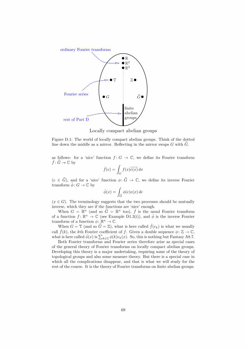
ordinary Fourier transforms
Fourier series
rest of Part D
RR2
R3
T Z
G G
finiteabeliangroups
Locally compact abelian groups
Figure D.1: The world of locally compact abelian groups. Think of the dottedline down the middle as a mirror. Reflecting in the mirror swaps G with G.
as follows: for a ‘nice’ function f : G → C, we define its Fourier transformf : G→ C by
f(e) =
∫G
f(x)e(x) dx
(e ∈ G), and for a ‘nice’ function φ : G → C, we define its inverse Fouriertransform φ : G→ C by
φ(x) =
∫G
φ(e)e(x) de
(x ∈ G). The terminology suggests that the two processes should be mutuallyinverse, which they are if the functions are ‘nice’ enough.
When G = Rn (and so G = Rn too), f is the usual Fourier transformof a function f : Rn → C (see Example D1.3(i)), and φ is the inverse Fouriertransform of a function φ : Rn → C.
When G = T (and so G = Z), what is here called f(ek) is what we usually
call f(k), the kth Fourier coefficient of f . Given a double sequence φ : Z → C,what is here called φ(x) is
∑k∈Z φ(k)ek(x). So, this is nothing but Fantasy A8.7.
Both Fourier transforms and Fourier series therefore arise as special casesof the general theory of Fourier transforms on locally compact abelian groups.Developing this theory is a major undertaking, requiring some of the theory oftopological groups and also some measure theory. But there is a special case inwhich all the complications disappear, and that is what we will study for therest of the course. It is the theory of Fourier transforms on finite abelian groups.
69
D2 The dual of a finite abelian group
For the lecture of Monday 24 March. (Lecture of Thu 20 March is cancelled)
Maybe you’re fed up with fussy analytic conditions: this function is continu-ously differentiable, that series is absolutely summable, and so on. If so, the lastfew lectures are for you. They will show you a world in which Fourier analysisworks beautifully without any analytic conditions at all.
Everything will be developed from the ground up, assuming only some ba-sic group theory. I will not assume any definitions, notation or results fromSection D1.
Definition D2.1 We denote by S the multiplicative group {z ∈ C : |z| = 1}.
Note that z = z−1 for z ∈ S.When we do Fourier analysis on finite abelian groups, we will always use
multiplicative notation for our groups (even though the locally compact abeliangroups in Section D1 were written additively). It’s only notation.
Lemma D2.2 Let G be a group. Then the set
G = {homomorphisms G→ S}
is a group under the following operations:
• the product of e1, e2 ∈ G is the product function e1 · e2 (defined as inNotation A3.3);
• the inverse of e ∈ G is e (again, defined as in Notation A3.3);
• the identity is the constant function 1.
Proof The set of all functions G → S is certainly a group under these opera-tions. We show that G is a subgroup of this group, that is:
• if e1, e2 : G→ S are homomorphisms then so is e1 · e2;
• if e : G→ S is a homomorphism then so is e;
• the constant function 1: G→ S is a homomorphism.
For the first one, if e1, e2 ∈ G then for all x, y ∈ G,
(e1 · e2)(xy) = e1(xy)e2(xy) (by definition of e1 · e2)
= e1(x)e1(y)e2(x)e2(y) (since e1 and e2 are homomorphisms)
= e1(x)e2(x)e1(y)e2(y) (since S is abelian)
= (e1 · e2)(x) · (e1 · e2)(y) (by definition of e1 · e2),
so e1 · e2 is a homomorphism. The arguments for e and 1 are similar (butsimpler). �
Definition D2.3 Let G be a finite abelian group. A character of G is ahomomorphism G → S. The character group or Pontryagin dual of G isthe group G.
70
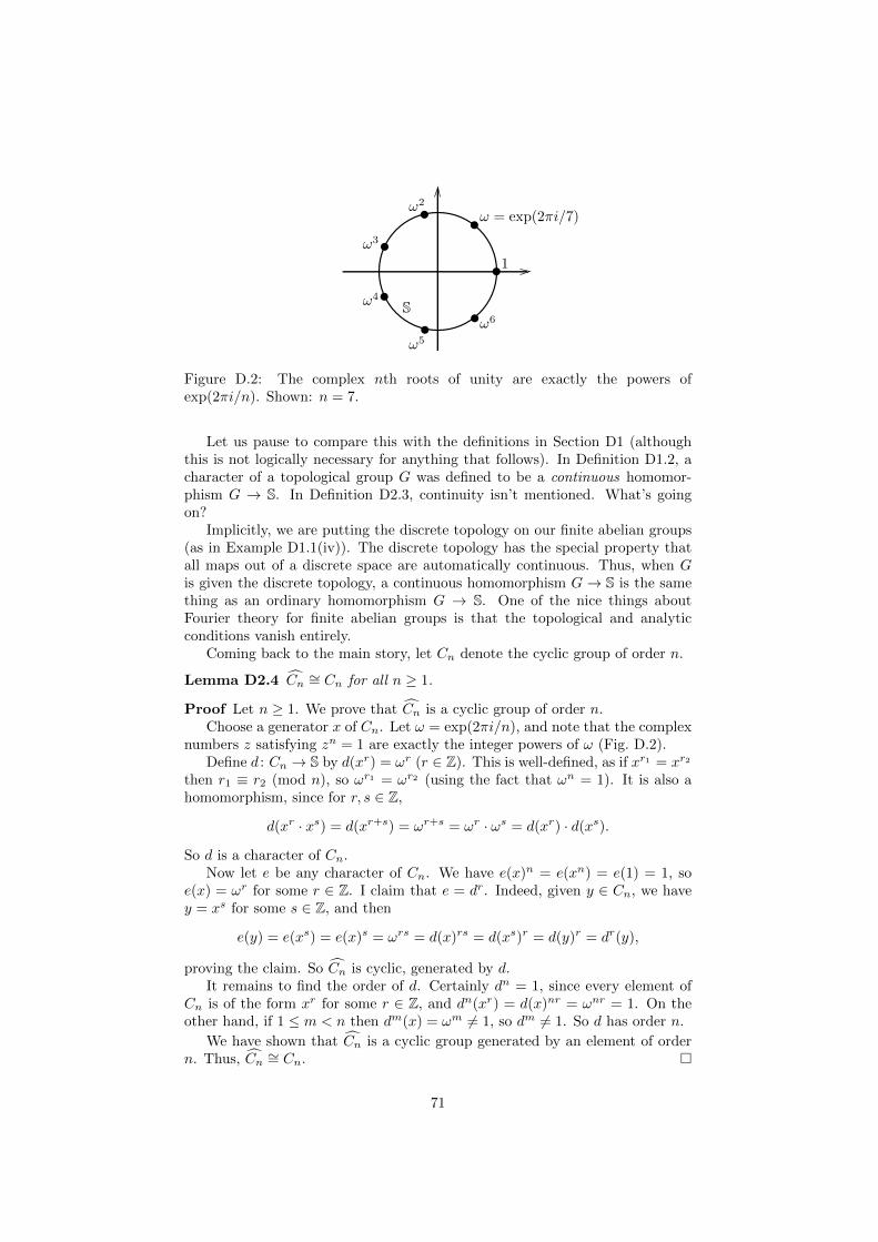
S
1
ω = exp(2πi/7)ω2
ω3
ω4
ω5
ω6
Figure D.2: The complex nth roots of unity are exactly the powers ofexp(2πi/n). Shown: n = 7.
Let us pause to compare this with the definitions in Section D1 (althoughthis is not logically necessary for anything that follows). In Definition D1.2, acharacter of a topological group G was defined to be a continuous homomor-phism G → S. In Definition D2.3, continuity isn’t mentioned. What’s goingon?
Implicitly, we are putting the discrete topology on our finite abelian groups(as in Example D1.1(iv)). The discrete topology has the special property thatall maps out of a discrete space are automatically continuous. Thus, when Gis given the discrete topology, a continuous homomorphism G→ S is the samething as an ordinary homomorphism G → S. One of the nice things aboutFourier theory for finite abelian groups is that the topological and analyticconditions vanish entirely.
Coming back to the main story, let Cn denote the cyclic group of order n.
Lemma D2.4 Cn ∼= Cn for all n ≥ 1.
Proof Let n ≥ 1. We prove that Cn is a cyclic group of order n.Choose a generator x of Cn. Let ω = exp(2πi/n), and note that the complex
numbers z satisfying zn = 1 are exactly the integer powers of ω (Fig. D.2).Define d : Cn → S by d(xr) = ωr (r ∈ Z). This is well-defined, as if xr1 = xr2
then r1 ≡ r2 (mod n), so ωr1 = ωr2 (using the fact that ωn = 1). It is also ahomomorphism, since for r, s ∈ Z,
d(xr · xs) = d(xr+s) = ωr+s = ωr · ωs = d(xr) · d(xs).
So d is a character of Cn.Now let e be any character of Cn. We have e(x)n = e(xn) = e(1) = 1, so
e(x) = ωr for some r ∈ Z. I claim that e = dr. Indeed, given y ∈ Cn, we havey = xs for some s ∈ Z, and then
e(y) = e(xs) = e(x)s = ωrs = d(x)rs = d(xs)r = d(y)r = dr(y),
proving the claim. So Cn is cyclic, generated by d.It remains to find the order of d. Certainly dn = 1, since every element of
Cn is of the form xr for some r ∈ Z, and dn(xr) = d(x)nr = ωnr = 1. On theother hand, if 1 ≤ m < n then dm(x) = ωm 6= 1, so dm 6= 1. So d has order n.
We have shown that Cn is a cyclic group generated by an element of ordern. Thus, Cn ∼= Cn. �
71
Next recall that any two groups G1 and G2 have a product (also called a‘direct product’) G1 ×G2.
Lemma D2.5 G1 ×G2∼= G1 × G2 for all finite abelian groups G1 and G2.
Proof Sheet 5. �
Fact D2.6 Every finite abelian group is isomorphic to Cn1 × Cn2 × · · · × Cnk
for some k, n1, n2, . . . , nk ≥ 1.
This is part of the classification theorem for finite abelian groups, which youmay have met in other courses.
Putting together the last three results gives:
Proposition D2.7 G ∼= G for every finite abelian group G.
Proof This follows from Lemma D2.4, Lemma D2.5 and Fact D2.6. �
This proposition is the reason why the finite abelian groups were drawn onthe central dotted line (the ‘mirror’) of Figure D.1.
Remark D2.8 For a given G, there is usually no canonical (i.e. God-given)
isomorphism G→ G. In order to construct an isomorphism, you have to makesome arbitrary choice, of the same kind you make when tossing a coin or choosinga basis for a vector space.
72
D3 Fourier transforms on a finite abelian group
For the lecture of Thursday 27 March
First we’ll make some definitions analogous to the definitions for Fourier series.Then we’ll prove some results analogous to results on Fourier series. We’lldiscover that life is much easier on a finite abelian group than on the circle.
For the rest of this section, let G be a finite abelian group.
Definition D3.1 i. Given a set X, write Fn(X) = {functions X → C}.
ii. For f ∈ Fn(G), write∫Gf(x) dx = 1
#G
∑x∈G f(x).
iii. For f, g ∈ Fn(G), write 〈f, g〉 =∫Gf(x)g(x) dx.
In (i), Fn(X) is a vector space over C, via the usual addition and scalarmultiplication of functions (as in Notation A3.3).
In (ii), the factor 1#G ensures that
∫G
1 dx = 1, just as∫T 1 dx = 1. So the
integral of a function on G can be thought of as its mean value, just as forfunctions on T.
We now establish some elementary properties of integration, directly analo-gous to those for ordinary integration stated in Lemma A3.4.
Lemma D3.2 i. For any functions f, g : G→ C,∫G
(f + g)(x) dx =
∫G
f(x) dx+
∫G
g(x) dx.
ii. For any function f : G→ C and c ∈ C,∫G
(cf)(x) dx = c
∫G
f(x) dx.
iii. For any function f : G→ C,∫G
f(x) dx =
∫G
f(x) dx.
Proof For (i), let f, g ∈ Fn(G). Then∫G
(f + g)(x) dx =
∫G
(f(x) + g(x)) dx (by definition of f + g)
=1
#G
∑x∈G
(f(x) + g(x)) (by definition of
∫G
)
=1
#G
∑x∈G
f(x) +1
#G
∑x∈G
g(x)
=
∫G
f(x) dx+
∫G
g(x) dx (by definition of
∫G
).
Similar arguments prove parts (ii) and (iii). �
73
Lemma D3.3 〈·, ·〉 is an inner product on Fn(G).
Proof This is straightforward, using Lemma D3.2. (Compare your solution toSheet 1, q.6(i).) �
Note that 〈·, ·〉 is a genuine inner product; that is, if 〈f, f〉 = 0 then f = 0.(Contrast the comments after Lemma A6.2.) This is because for f ∈ Fn(G),
〈f, f〉 =1
#G
∑x∈G|f(x)|2,
and if this is 0 then f(x) = 0 for all x ∈ G.In the proof of Lemma A7.4 (which stated that the characters of T are
orthonormal), it was shown in passing that∫T ek(x) dx is 1 if k = 0 and 0
otherwise. Something very similar holds for finite abelian groups.
Lemma D3.4 Let e ∈ G. Then∫G
e(x) dx =
{1 if e = 1
0 otherwise.
Remember that the elements of G are homomorphisms, so the ‘1’ in ‘e = 1’means the constant function 1 from G to C.
Proof If e = 1 then∫Ge(x) dx = 1 (as noted after Definition D3.1).
If e 6= 1, choose y ∈ G such that e(y) 6= 1. Then∫G
e(x) dx =1
#G
∑x∈G
e(x) =1
#G
∑z∈G
e(yz)
since as x runs over G, z = y−1x runs over G too. (Morally, this is integrationby substitution; we’re substituting x = yz.) So∫
G
e(x) dx =1
#G
∑z∈G
e(y)e(z) = e(y)
∫G
e(x) dx.
But e(y) 6= 1, so∫Ge(x) dx = 0. �
Proposition D3.5 The characters of G are orthonormal: for e1, e2 ∈ G,
〈e1, e2〉 =
{1 if e1 = e2
0 otherwise.
(Compare Lemma A7.4, the analogous result on T.)
Proof Let e1, e2 ∈ G. Since e2 is the inverse of e2 in G, we have e1e2 ∈ G. ByLemma D3.4,
〈e1, e2〉 =
∫G
(e1e2)(x) dx =
{1 if e1e2 = 1
0 otherwise=
{1 if e1 = e2
0 otherwise. �
74
Definition D3.6 Let f ∈ Fn(G). The Fourier transform of f is the function
f ∈ Fn(G) defined by f(e) = 〈f, e〉 (e ∈ G).
(Compare: for Fourier series, f(k) = 〈f, ek〉.)Note that we’ve defined the Fourier transform of any function on G! In our
simple world of finite groups, there’s no integrability to worry about.
Proposition D3.7 For all φ ∈ Fn(G),
φ =
(∑e∈G
φ(e) · e)∧
(The right-hand side means f where f =∑e∈G φ(e) · e. This alternative
notation is simply for typesetting convenience, to avoid very wide hats.)
The sum on the right-hand side is a finite sum, since G ∼= G (by Proposi-tion D2.7) and G is finite. Unlike the circle, G has only finitely many characters.
Proof Both sides of this equation are functions on G, so to prove equality, weneed to take an arbitrary element e′ of G and show that evaluating each side ate′ gives the same result.
Let e′ ∈ G. Then(∑e∈G
φ(e) · e)∧
(e′) =⟨∑
e
φ(e) · e, e′⟩
=∑e
φ(e)〈e, e′〉 (by Lemma D3.3)
= φ(e′) (by orthonormality). �
This result is similar to the ‘Moreover’ part of Proposition C2.1, which statedthat for ‘nice’ c ∈ Fn(Z), we have c =
(∑k∈Z ckek
)∧.
Recall that Fn(G) is a vector space over C.
Lemma D3.8 dim(Fn(G)) = #G.
Proof For each x ∈ G, define δx ∈ Fn(G) by
δx(y) =
{1 if y = x
0 otherwise
(y ∈ G). The family (δx)x∈G spans Fn(G), since if f ∈ Fn(G) then f =∑x∈G f(x)δx (check!). It is also linearly independent, since if (cx)x∈G is a
family of complex numbers such that∑x∈G cxδx = 0, then for each y ∈ G we
have
0 =
(∑x∈G
cxδx
)(y) =
∑x∈G
cxδx(y) = cy.
So it is a basis. �
Lemma D3.8 doesn’t really have an analogue in the world of Fourier series(that is, Fourier theory on the circle group T).
75
Theorem D3.9 The characters of G form an orthonormal basis of Fn(G).
Proof By Proposition D3.5, the characters are orthonormal. In particular, theyare linearly independent, so the subspace of Fn(G) that they span has dimension
#G. But #G = #G = dim(Fn(G)) by Proposition D2.7 and Lemma D3.8, sotheir span is Fn(G). �
Hence every function on G is a ‘trigonometric polynomial’ (a finite linearcombination of characters). This makes Fourier analysis on finite groups con-siderably simpler than Fourier analysis on the circle.
For a function f : G→ C, the analogue of the Fourier series of f is the sum∑e∈G f(e)e. Since this sum is finite, there is no question of convergence; either
it is equal to f , or it is not. The next result says that it is.
Corollary D3.10 For all f ∈ Fn(G), f =∑e∈G f(e)e.
Proof By Theorem D3.9, f =∑e∈G〈f, e〉e; but f(e) = 〈f, e〉 by definition. �
So we can reconstruct a function from its Fourier transform. For Fourierseries, we had to work hard to prove that!
Since we can reconstruct a function from its Fourier transform, if two func-tions have the same Fourier transform then they must in fact be the same:
Corollary D3.11 Let f, g ∈ Fn(G). If f = g then f = g.
Proof Follows from Corollary D3.10. �
This is the (simpler) analogue of Corollary B8.5; see also Remark C4.3.
76
D4 Fourier inversion on a finite abelian group
For the lecture of Monday 31 March
Throughout this section, let G be a finite abelian group.
Definition D4.1 For φ ∈ Fn(G), define φ ∈ Fn(G) by φ =∑e∈G φ(e)e.
The upside-down hat is meant to suggest the opposite of the Fourier trans-form. It is pronounced ‘check’ (as in ‘phi-check’).
Remark D4.2 Suppose we were dealing with the circle T rather than a finiteabelian group G. We have T = Z (as in Section D1), so φ would be an elementof Fn(Z), that is, a double sequence c = (ck)k∈Z. Then c is notation for thefamiliar expression
∑k∈Z ckek.
Fantasy A8.7 comes true in the setting of finite abelian groups. (No fussyanalytical details!) This is the content of the following theorem.
Theorem D4.3 The maps
Fn(G)ˆ( ) //
Fn(G)ˇ( )
oo
are linear and mutually inverse. In particular, the vector spaces Fn(G) and
Fn(G) are isomorphic.
Proof Corollary D3.10 states thatˇf = f for all f ∈ Fn(G), and Proposi-
tion D3.7 states that ˆφ = φ for all φ ∈ Fn(G). So ˆ( ) and ˇ( ) are mutually
inverse. The map ˆ( ) is linear since 〈·, ·〉 is linear in the first argument; so its
inverse ˇ( ) is linear too. Hence ˆ( ) and ˇ( ) define an isomorphism of vectorspaces. �
Definition D4.4 For f ∈ Fn(G), define ‖f‖2 =√〈f, f〉.
This defines a norm ‖ · ‖2 on Fn(G), since 〈·, ·〉 is an inner product.
Theorem D4.5 (Parseval for finite abelian groups) For all f ∈ Fn(G),
‖f‖2 =
√∑e∈G
|f(e)|2.
Proof By Corollary D3.10, f =∑e∈G f(e)e. So by orthogonality of the char-
acters,
‖f‖22 = 〈f, f〉 =∑e∈G
|f(e)|2.�
We know from Theorem D4.3 that the function ˆ( ) : Fn(G) → Fn(G) is anisomorphism of vector spaces. We’d like to say that it’s also an isomorphism ofmetric spaces, that is, distance-preserving: ‖f‖2 = ‖f‖2 for all f ∈ Fn(G). Butthe right-hand side is not yet defined. So we make some definitions:
77

Definition D4.6 i. For φ ∈ Fn(G), define∫Gφ(e) de =
∑e∈G φ(e) ∈ C.
ii. For φ, ψ ∈ Fn(G), define 〈φ, ψ〉 =∫Gφ(e)ψ(e) de ∈ C.
iii. For φ ∈ Fn(G), define ‖φ‖2 =√〈φ, φ〉.
Compare and contrast (i) with Definition D3.1(ii): here, there is no factorof 1
#G . This is to make the following true:
Corollary D4.7 (Parseval, restated) For all f ∈ Fn(G),
‖f‖2 = ‖f‖2.
Proof This is a restatement of Theorem D4.5, since for φ ∈ Fn(G) we have
‖φ‖2 =√∑
e∈G |φ(e)|2. �
The characters of G are functions G→ C with certain properties. Are thereenough such functions to tell different points of G apart? That is, if x and yare two different points in G, can we find a character e such that e(x) and e(y)are different?
The answer is yes, and it’s now easy for us to prove. But it’s not so easy toprove from scratch: try it!
Proposition D4.8 (Characters separate points) Let x, y ∈ G with x 6= y.
Then there is some e ∈ G such that e(x) 6= e(y).
Proof Suppose that e(x) = e(y) for all e ∈ G. Since x 6= y, there is somef ∈ Fn(G) such that f(x) 6= f(y). (E.g. define f by f(x) = 1 and f(z) = 0 forall z 6= x.) Then by Corollary D3.10,
f(x) =∑e∈G
f(e)e(x) =∑e∈G
f(e)e(y) = f(y),
a contradiction. �
Remark D4.9 We know from Proposition D2.7 that G ∼= G ∼= G, so G ∼=
G.
But for all we know so far, there is no canonical choice of isomorphism G→ G.
(Recall Remark D2.8.) However, the next result tells us that although thereis no canonical isomorphism between a group and its single dual, there is acanonical isomorphism between a group and its double dual.
Theorem D4.10 For x ∈ G, define evx ∈ Fn(G) by
evx(e) = e(x)
(e ∈ G). Then evx ∈G for all x ∈ G, and the map
G −→ G
x 7−→ evx
is an isomorphism of groups.
78
Proof For each x ∈ G, the function evx is a homomorphism G → S: indeed,for all e1, e2 ∈ G, we have
evx(e1 · e2) = (e1 · e2)(x) (by definition of evx)
= e1(x)e2(x) (by definition of e1 · e2)
= evx(e1) evx(e2) (by definition of evx).
This means we can define a function ev : G→ G by ev(x) = evx (x ∈ G).
This function ev is a homomorphism. Indeed,
ev is a homomorphism
⇐⇒ ∀x, y ∈ G, ev(xy) = ev(x) · ev(y)
⇐⇒ ∀x, y ∈ G, evxy = evx · evy
⇐⇒ ∀x, y ∈ G,∀e ∈ G, evxy(e) = (evx · evy)(e)
⇐⇒ ∀x, y ∈ G,∀e ∈ G, evxy(e) = evx(e) · evy(e)
⇐⇒ ∀x, y ∈ G,∀e ∈ G, e(xy) = e(x) · e(y),
which is true. So reading the implications from bottom to top, ev is a homo-morphism.
Next, ev : G → G is injective. For let x, y ∈ G and suppose that ev(x) =
ev(y). Then evx = evy, that is, evx(e) = evy(e) for all e ∈ G. But charactersseparate points (Proposition D4.8), so x = y.
Finally, ev : G → G is surjective, since ev is injective, #G = #G = #
G by
Proposition D2.7, and an injection from one finite set to another set of the samecardinality is always surjective, by the pigeonhole principle. �
This is Pontryagin’s duality theorem (Theorem D1.4) in the special case offinite abelian groups.
We have now proved analogues of all the main results on Fourier series inthe setting of finite abelian groups. We have also proved the central theoremof abstract Fourier analysis (Pontryagin duality) in this simplified setting. Andwe have done all this in just a few pages, calling on nothing more than basicgroup theory.
∗ ∗ ∗
79