Embed Size (px)
Citation preview

Four Types of Ignorance
Lars Peter Hansen and Thomas J. Sargent∗
May 18, 2014
Abstract
This paper studies alternative ways of representing uncertainty about a law of mo-
tion in a version of a classic macroeconomic targetting problem of Milton Friedman
(1953). We study both “unstructured uncertainty” – ignorance of the conditional
distribution of the target next period as a function of states and controls – and more
“structured uncertainty” – ignorance of the probability distribution of a response co-
efficient in an otherwise fully trusted specification of the conditional distribution of
next period’s target. We study whether and how different uncertainties affect Fried-
man’s advice to be cautious in using a quantitative model to fine tune macroeconomic
outcomes.
1 Introduction
“As Josh Billings wrote many years ago, “The trouble with most folks isn’t so
much their ignorance, as knowing so many things that ain’t so.” Pertinent as
this remark is to economics in general, it is especially so in monetary economics.”
Milton Friedman (1965) 1
Josh Billings may never have said that. Some credit Mark Twain. Despite, or maybe
because of the ambiguity about who said them, those words convey the sense of calculations
∗We thank Harald Uhlig for thoughtful comments and David Evans and Paul Ho for excellent researchassistance.
1From the forward to Phillip Cagan’s Determinants and Effects of Changes in the Stock of Money,1875-1960, Columbia University Press, New York and London, 1965. page xxiii.
1

that Milton Friedman (1953) used to advise against using quantitative macroeconomic mod-
els to “fine tune” an economy. Ignorance about details of an economic structure prompted
Friedman to recommend caution.
We use a dynamic version of Friedman’s model as a laboratory within which we study
the consequences of four ways that a policy maker might confess ignorance. One of these
corresponds to Friedman’s, while the other three go beyond Friedman’s. Our model states
that a macroeconomic authority takes an observable state variable Xt as given and chooses
a control variable Ut that produces a random outcome for Xt+1:
Xt+1 = κXt + βUt + αWt+1. (1)
The shock process W is an iid sequence of standard normally distributed random variables.
We interpret the state variable Xt+1 as a deviation from a target, so ideally the policy
maker wants to set Xt+1 = 0, but the shock Wt+1 prevents this.
Friemdan framed the choice between “doing more” and “doing less” in terms of the
slope of the response of a policy maker’s decision Ut to its information Xt about the state
of the economy. Friedman’s purpose was to convince policy makers to lower the slope. He
did this by comparing optimal policies for situations in which the policy maker knows β
and in which it doesn’t know β.
For working purposes, it is useful tentatively to classify types of ignorance into not
knowing (i) response coefficients (β), and (ii) conditional probability distributions of ran-
dom shocks (Wt+1). Both categories of unknowns potentially reside in our model, and we’ll
study the consequences of both types of ignorance. As we’ll see, confining ignorance to
not knowing coefficients puts substantial structure on the source of ignorance by trusting
significant parts of a specification. Not knowing the shock distribution translates into not
knowing the conditional distribution of Xt+1 given time t information and so admits a
potentially large and less structured class of misspecifications.
After describing a baseline case in which a policy maker completely trusts specification
(1), we study the consequences of four ways of expressing how a policy maker might distrust
that model.2
I. A “Bayesian decision maker” doesn’t know the coefficient β but trusts a prior prob-
ability distribution over β. (This was Friedman’s way of proclaiming model uncer-
2Our preoccupation within enumerating types of ignorance and ambiguity here and in Hansen andSargent (2012) is inspired by Epson (1947).
2

tainty.)
II. A “robust Bayesian decision maker” uses operators of Hansen and Sargent (2007) to
express distrust of a prior distribution for the response coefficient β. The operators tell
the decision maker how to make cautious decisions by twisting the prior distribution
in a direction that increases probabilities of β’s yielding lower values.
III. A “robust decision maker” uses either the multiplier or the constraint preferences of
Hansen and Sargent (2001) to express his doubts about the probability distribution
of Wt+1 conditional on Xt and a decision Ut implied by model (1). Here an operator
of Hansen and Sargent (2007) twists the conditional distribution of Xt+1 to increase
probabilities of Xt+1 values that yield low continutation utilities.
IV. A robust decision maker asserts ignorance about the same conditional distribution
mentioned in item (III) by adjusting an entropy penalty in a way that Petersen et al.
(2000) used to express a decision maker’s desire for a decision rule that is robust at
least to particular alternative probability models.
Approaches (I) and (II) are ways of ‘not knowing coefficients’ while approaches (III)
and (IV) are ways of ‘not knowing a shock distribution.’ We compare how these types
of ignorance affect Friedman’s conclusion that ignorance should induce caution in policy
making.3
2 Baseline model without uncertainty
Following Friedman, we begin with a decision maker who trusts model (1). The decision
maker’s objective function at date zero is
−1
2
∞∑t=0
exp(−δt)E[(Xt)
2|X0 = x]
=− 1
2
∞∑t=0
exp[−δ(t+ 1)]E[(κXt + βUt)
2|X0 = x]
− 1
2x2 − α2 exp(−δ)
2[1− exp(−δ)], (2)
3Approaches (I), (II), and (III) have been applied in macroeconomics and finance, but with the exceptionof Hansen et al. (2014), approach (IV) has not.
3

where δ > 0 is a discount rate. The decision maker chooses Ut as a function of Xt to
maximize (2) subject to the sequence of constraints (1). The optimal decision rule
Ut = −κβXt (3)
attains the following value of the objective function (2):
−1
2x2 − α2 exp(−δ)
2[1− exp(−δ)].
Under decision rule (3) and model (1), Xt+1 = αWt+1.
In subsequent sections, we study how two types of ignorance change the decision rule
for Ut relative to (3):
• Ignorance about β.
• Ignorance about the probability distribution of Wt+1 conditional on information avail-
able at time t.
3 Friedman’s Bayesian expression of caution
This section sets Friedman’s analysis within a perturbation of model (1). We study how
the decision maker adjusts Ut to offset adverse effects of Xt on Xt+1 when he does not
know the response coefficient β. Does he do a lot or a little? Friedman’s purpose was to
advocate doing less relative to the benchmark rule (3) for setting Ut.
We replace (1) with
Xt+1 = κXt + βtUt + αWt+1, (4)
where the decision maker believes that {βt} is iid normal with mean µ and variance σ2,
which we write
βt ∼ N (µ, σ2). (5)
An iid prior asserts that information about βt is useless for making inferences about βt+j
for j > 0, thus ruling out the possibility of learning.4
4de Finetti (1937) introduced exchangeability of a stochastic process as a way to make rooom forlearning. Kreps (1988, ch. 11) described de Finetti’s work as a foundation of statistical learning. Krepsoffered a compelling explanation of why an iid prior excludes learning. Prescott (1972) departed from iidrisk to create a setting in which a decision maker designs experiments because he wants to learn. ? study
4

Let x∗ denote a next period value.5 Model (4)–(5) implies that the conditional density
for x∗ is normal with mean κx+ µu and variance σ2u2 + α2. Conjecture a value function
V (x) = −1
2ν1x
2 − 1
2ν0
that satisfies the Bellman equation:
V (x) = maxu−{
exp(−δ)2
ν1(κx+ µu)2 − exp(−δ)2
ν1σ2u2 − exp(−δ)
2ν1α
2 − exp(−δ)2
ν0 −1
2x2}.
(6)
First-order conditions with respect to u imply that
− exp ν1[µ(κx+ µu) + σ2u
]= 0
so that the optimal decision rule is
u = −(
µκ
µ2 + σ2
)x, (7)
which has the same form as the rule that Friedman derived for his static model. Because
µκ
µ2 + σ2<κ
µ,
caution shows up in decision rule (7) when σ2 > 0, indicating how Friedman’s Bayesian
decision rule recommends “doing less” than the known-β rule (3).6
4 Robust Bayesians
A robust Bayesian is unsure of his prior and therefore pursues a systematic analysis of the
sensitivity of expected utility to perturbations of his prior. Aversion to prior uncertainty
induces a robust Bayesian decision maker to calculate a lower bound on expected utility
over a set of priors, and to investigate how decisions affect that lower bound. We describe
two recursive implementations.
a setting with a robust decision maker who experiments and learns.5From now on, upper case letters denote random vectors (subscripted by t) and lower case letters are
realized values.6See Tetlow and von zur Muehlen (2001) and Barlevy (2009) for discussions of whether adjusting for
model uncertainty renders policy more or less aggressive.
5

In this section, we modify the Bayesian model of section 3. The decision maker still
believes that βt is an iid scalar process. But now he doubts his prior distribution (5) for
βt. He expresses his doubts about (5) by using one of two operators of Hansen and Sargent
(2007) to replace the conditional expectation operator in Bellman equation (6). We assume
that the decision maker confronts ambiguity about the baseline normal distribution for {βt}that is not diminished by looking at past history. The decision maker’s uncertainty about
the distribution of βt is not tied to his uncertainty about the distribution of βt+1 except
through the specification of the baseline normal distribution. In this paper, we deliberately
close down learning for simplicity. In other papers (e.g., see Hansen and Sargent (2007,
2010)), we have applied the methods used here to environments in which a decision maker
learns about hidden Markov states.
4.1 T2 and C2 operators as indirect utility functions
We define two operators, T2, expressing “multiplier preferences”, and C2, expressing a type
of “constraint preferences” in the language of Hansen and Sargent (2001). A common
parameter θ appears in both operators. But in T2, θ is a fixed penalty parameter, while in
C2, θ is a Lagrange multipler, an endogenous object whose value varies with both the state
x and the decision u.
4.1.1 Relative entropy of a distortion to the density of βt
Let φ(β;µ, σ2) denote the Gaussian density for β assumed in Friedman’s model. The
relative entropy of an alternative density f(β;x, u) with respect to the benchmark density
φ(β;µ, σ2) is
ent(f, φ) =
∫m(β;x, u) log(m(β;x, u))φ(β;µ, σ2)d β
where m(β;x, u) is the likelihood ratio
m(β;x, u) =
(f(β;x, u)
φ(β;µ, σ2)
).
Relative entropy is thus an expected log-likelihood ratio evaluated with respect to the
distorted density f = mφ for β.
6

4.1.2 The T2 operator
Let θ ∈ [θ,+∞] be a fixed penalty parameter where θ > 0. Where V (β;x, u) is a value
function, the operator [T2V ](x, u) is the indirect utility function for the following problem:
[T2V ](x, u) = minm≥0,∫βmφ=1
[∫exp(−δ)V (x, β, u)m(β;x, u)φ(β;µ, σ2)dβ + θ ent(mφ, φ)
]= Eβ
(m(β;x, u) exp(−δ)V (x, β, u)
)+ θ ent(mφ, φ) (8)
where φ(β;µ, σ2) is a Gaussian density and the minimizer is m. The minimizing likelihood
ratio m satisfies the exponential twisting formula
m(β;x, u) ∝ exp
[−exp(−δ)
θV (x, β, u)
], (9)
with the factor of proportionality being the mathematical expectation of the object on
the right, so that m(β;x, u) integrates against φ to unity. The “worst-case” density for β
associated with [T2V ](x, u) is7
f(β;x, u) = m(β;x, u)φ(β;µ, σ2). (10)
Substituting the minimizing m into the right side of (8) and rearranging shows that the
T2 operator can be expressed as the indirect utility function
[T2V ](x, u) = −θ logE
(exp
[−exp(−δ)
θV (Xt, βt, Ut)
] ∣∣∣Xt = x, Ut = u
), (11)
where according to (5), βt ∼ N (µ, σ2). Equation (8) represents [T2V ](x, u) as the sum of
the expectation of V evaluated at the minimizing distorted density f = mφ plus θ times
entropy of the distorted density f . Associated with a fixed θ is an entropy
ent(mφ, φ)(x, u) =
∫m(β;x, u) log(m(β;x, u))φ(β;µ, σ2)d β (12)
that for a fixed θ evidently varies with x and u.
Remark 4.1. (Relationship to smooth ambiguity models) The operator (11) is an indirect
7Notice that the minimizing density (10) depends on both the control law u and the endogenous state x.In subsection 4.5, we describe how to construct another representation of the worst-case density in whichthis dependence is replaced by dependence on an additional state variable that is exogenous to the decisionmaker’s choice of control u.
7

utility function that emerges from solving a penalized minimization problem over a contin-
uum of probability distortions. The smooth ambiguity models of Klibanoff et al. (2005, 2009)
posit a specification resembling and generalizing (11), but without any reference to such a
minimization problem. In the context of a random coefficient model like (4), Klibanoff
et al. would use one concave function to express aversion to the risk associated with ran-
domness in the shock Wt+1 but conditioned on βt, on the one hand, and another concave
function to express aversion to ambiguity about the distribution of βt, on the other hand.
The functional form (11) emerges from the formulation of Klibanoff et al. (2005) if we
use a quadratic function for aversion to risk and an exponential function for aversion to
ambiguity about the probability distribution of βt.
4.1.3 The C2 operator
For the T2 operator, θ is a fixed parameter that penalizes the m-choosing agent in problem
(8) for increasing entropy. The minimizing decision maker in problem (8) can change
entropy but at a marginal cost θ.
For the C2 operator, instead of a fixed θ, there is a fixed level η ≥ 0 of entropy that
the probability-distorting minimizer cannot exceed. The C2 operator is the indirect utility
function defined by the following problem:
[C2V ](x, u) = minm(β;x,u)≥0
∫exp(−δ)V (x, β, u)m(β;x, u)φ(β;µ, σ2)dβ (13)
where the minimization is subject to Eβm(β;x, u) = 1 and
ent(mφ, φ) ≤ η. (14)
The minimizing choice of m again obeys equation (10), except that θ is not a fixed penalty
parameter, but instead a Lagrange multiplier on constraint (13). Now the Lagrange mul-
tiplier θ varies with x and u, not entropy.
Next we shall use T2 or C2 to design a decision rule that is robust to a decision maker’s
doubts about the probability distribution of βt.
8

4.2 Multiplier preference adjustment for doubts about distribu-
tion of βt
Here the decision maker’s (robust) value function V satisfies a functional equation (15) cast
in terms of intermediate objects that we construct in the following steps:
• Average over the probability distribution of the random shock Wt+1 to compute
V (x, β, u) = E[V (κXt + βtUt + αWt+1)
∣∣∣Xt = x, βt = β, Ut = u],
where W ∼ N (0, 1).
• Next, use definition (11) to average V over the distribution of βt and thereby compute
the indirect utility function [T2V ](x, u).
• Choose u to attain the right side of
V (x) = maxu−1
2x2 + [T2]
(V (x, u)
). (15)
• Iterate to convergence to construct a fixed point V (·).
4.3 Constraint preference adjustment for doubts about distribu-
tion of βt
Here we use the same iterative procedure described in subsection 4.2 except that we replace
the steps described in the second and third bullet points with
• Use definition (13) of C2 to average V over random βt and thereby compute [C2](V (x, u)
).
• Choose u to attain the right side of
V (x) = maxu−1
2x2 + [C2]
(V (x, u)
). (16)
Appendix B describes how we approximate V and V in Bellman equations (15) and (16).
9

4.4 Examples
Figures 1–3 show robust decision rules that attain the right sides of (15) and (16) for an
infinite horizon model with parameters set at µ = 1, σ = 1, δ = .1, α = .6, κ = .8. We
analyze a two period version in appendix A. Figures 1, 2, and 4 show robust decision rules
that attain the right side of (15) while figure 3 describes decision rules that attain the right
side of (16).
Figure 1 shows decision rules for u as a function of x for θ values of .5 and 1, as well
as for the θ = +∞ value associated with Friedman’s Bayesian rule (7) with σ2 > 0 and
the benchmark no-ignorance rule (3) associated with σ2 = 0. With θ < +∞, the robust
decision rules are non-monotonic. They show caution relative to Friedman’s rule, and
increasing caution for larger values of |x|. For low values of |x|, the robust rules are close
to Friedman’s Bayesian rule, but for large values of |x|, the robust rules are much more
cautious. For the two-period model analyzed in appendix A, the worst-case distribution of
βt remains Gaussian. For the infinite horizon model, the worst-case distributions seem very
close to Gaussian. Figure 2 shows means and variances of worst-case probability densities
(in the top two panels) and relative entropies of the worst-case distributions with respect to
the density N (µ, σ2) under the approximating model, all as functions of x. As x increases
in absolute value, the mean of the worst-case distribution of β decreases, indicating that
the policy is less effective. As |x| increases, the worst-case variance increases at first, but
eventually it decreases. The shape of entropy as a function of x, shown in the bottom panel
of figure 2, sheds light on why the worst-case variance ultimately starts decreasing. As |x|increases, at first entropy increases too, reaching a maximum and then slowly decreasing.
Notice how the “wings” in the two robust decision rules in figure 1 and the worst-case
variances in figure 2 mirror those in the graph of entropy as a function of x in the bottom
panel of figure 2. Figure 3 plots two robust decision rules and stationary distributions of
Xt under those decision rules and the baseline model (1). The graphs are for two levels of
σ: σ = .75 and σ = 1.5. The graphs reveal that the ‘wings’ in the decision rules do not
occur too far out in the tails of the stationary distribution.
10

−8 −6 −4 −2 0 2 4 6 8x
−6
−4
−2
0
2
4
6
u
Figure 1: The β known and Friedman’s Baysian decision rules (the two linear rules), and
also robust decision rules that solve maxu−12x2 + [T2]
(V (x, u)
)for two values of θ.
−8 −6 −4 −2 0 2 4 6 80.0
0.2
0.4
0.6
0.8
1.0
Mean
−8 −6 −4 −2 0 2 4 6 80.00.10.20.30.40.50.60.70.8
Vari
ance
−8 −6 −4 −2 0 2 4 6 8x
0.00.10.20.30.40.50.60.70.80.9
Rela
tive E
ntr
opy
Figure 2: Top two panels: worst-case means and variances associated with decision rules
that solve maxu−12x2 + [T2]
(V (x, u)
)for various θ’s; lower panel: entropy as a function
of x.
11

−0.2
−0.15
−0.1
−0.05
0
0.05
0.1
0.15
u
σ = 1.5
−5 −4 −3 −2 −1 0 1 2 3 4 50
0.05
0.1
0.15
0.2
0.25
0.3
0.35
0.4
0.45
0.5
density
x
u(x)
density
−0.4
−0.2
0
0.2
0.4
u
σ = 0.5
−4 −3 −2 −1 0 1 2 3 40
0.2
0.4
0.6
0.8
density
x
u(x)
density
Figure 3: Robust decision rules and stationary distribution under approximating model under
those rules.
The robust decision rules that attain the right side of (16) are reported in the top panel
figure 4 for values of η of 0.1 and 0.4, as well as the non-robust η = 0 rule. The middle
and bottom panels show the associated worst-case means and variances, which for a given
entropy are constant functions of x. Here, with fixed entropy, the decision rules seem to
be linear.8 They are flatter (more cautious), the higher is entropy. The minimizing player
responds to an increase in entropy by increasing the variance and decreasing the mean of
βt, making policy both less effective and more uncertain. The robust (maximizing) decision
maker responds by making u less responsive to x. The constaint-preference robust Bayesian
decision rule looks like Friedman’s, except that it is even more cautious because of how the
robust Bayesian decision maker acts as if the mean of βt is lower and the variance of the
βt is larger than does Friedman’s Bayesian decision maker.9,10
Figure 5 shows that the Lagrange multiplier θ for the constraint preferences in (16)
increases apparently quadratically with |x|. For a given entropy η, the increase in the
“price of robustness” θ as |x| increases causes the “wings” that in the robust (15) decision
8In the two-period version of the model analyzed in appendix A we can prove that they are linear.9This behavior is familiar from what we have seen in other robust decision problems that we have
studied: in the sense that variance (noise about β) gets translated into a mean distortion.10Recall formula (7) for Friedman’s Bayesian decision rule and notice that
∂
∂µ
(µκ
µ2 + σ2
)=κ(σ2 − µ2)
(µ2 + σ2)2,
which says that depending on the sign of σ2−µ2, the absolute value of the response coefficient may increaseor decrease with an increase in µ. Notice that we have set µ = σ in our numerical, which makes this effectvanish. When σ2 = 0, an increase in µ causes the absolute value of the slope to decrease – the policy makerdoes less because the policy instrument is more effective.
12
rules displayed in the top panel of figure 1 to disappear in the (16) decision rules displayed
in figure 4.
Remark 4.2. In applying the C2 operator in recursion (16), we have imposed a fixed
entropy constraint period-by-period. That specification caused the “wings” associated with
recursion (15) to vanish. If instead we had imposed a single intertemporal constraint on
discounted entropy at time 0 and solved that entropy constraint for an associated Lagrange
multiplier θ, it would give rise to the fixed-θ decision rule associated with the T2 recursion
(15) having the “wings” discussed above. Our discussion of how entropy varies with x in
the fixed θ rule would then pertain to how a fixed discounted entropy would be allocated
across time and states conditioned on an initial realized state X0.
4.5 Another representation of worst-case densities
In subsection 4.1.2, we reported formula (10), which expresses a worst case m as a function
of the control u and the state x. This worst-case density emerges from a recursive version
of the max-min problem that fist maximizes over u, then minimizes over m.11,12 In this
section, we briefly describe some analytical dividends that accrue when it is possible to
form an alternative representation of a (sequence of) worst-case densities, an outcome that
requires that it be legitimate to replace max-min with min-max. We presume that current
and past values of {(Wt, βt−1)} along with an initial condition for X0 are observed when
the date t control Ut is decided.
The issue under consideration is whether it is possible to construct a Bayesian inter-
pretation of a robust decision rule. This requires a different representation of a worst-case
distribution than provided by formula (10), one that takes the form of a sequence of prob-
ability densities for βt, t ≥ 0. When enough additional assumptions are satisfied, this is
possible. Then it can be shown easily that the robust decision rule is an optimal deci-
sion rule for an ordinary Bayesian who takes this sequence of distributions as given.13 In
the applications described here, this sequence of worst-case distributions of βt has some
interesting features. In particular, although the baseline model asserts that the sequence
11The minimization is implicit when we use an indirect utility function expressed by applying a T2 orC2 operator, as we do in recursions (15) and (16),respectively.
12The type of analysis sketched in this section is presented in more detail in the context of infinite horizonlinear-quadratic models in Hansen and Sargent (2008, ch. 7).
13Establishing that a robust decision rule can be interpreted as an optimal decision rule for a Bayesianwith some prior distribution is needed to establish that a robust decision rule is “admissible” in the senseof Bayesian statistical decision theory.
13

βt, t ≥ 0 is iid, they are in general not iid under a worst-case model. Instead the worst-case
distribution for βt+1 that depends on current and past information.
4.5.1 Replacing max-min with min-max
A key first step in constructing such a worst-case model that supports such a Bayesian inter-
pretation of a robust rule involves verifying that exchanging the order of the minimization
and maximization in problem (8) or (13) leaves the associated value function unaltered.
If this is true, a Bellman-Isaacs condition for the associated zero-sum, two-player game is
said to be satisfied. That makes it possible to construct a representation of the worst-case
m of the form
m∗(β, x) = m[β, u(x), x], (17)
where u(x) is the robust control law. Given m∗, the robust decision rule u solves a dynamic
recursive version of Friedman’s Bayesian problem, except that m∗(βt, x)φ(βt;µ, σ2) replaces
the baseline model φ(βt;µ, σ2).
4.5.2 Application of “Big K, little k”
For our purpose here, it is troublesome that the state variable Xt, which appears as x in
(17) is endogenous in the sense that its future values are partly under the control of the
maximizing decision maker. This can be avoided by using a version of the macroeconomist’s
“Big K, little k” trick to represent the worst-case density in a way that puts it beyond
influence of the maximizing player.14 The idea is to start by recalling that ordinary dynamic
programming is a recursive method for solving a date zero problem originally cast in terms
of choices of sequences. When the Bellman-Isaacs condition is satisfied, we can use an
analogous mapping between date 0 problems cast in terms of sequences and problems
expressed recursively a la dynamic programming applies to two-person zero sum games like
the ones we are studying. That reasoning lets us also exchange orders between maximization
minimization at date 0 for a robust control problem cast in terms of choices of sequences.
We accomplish by inventing a new exogenous state variable process {Zt} whose evolution
is the same as that of Xt+1 “along an equilibrium path”, meaning “when the robust control
law is imposed”. But now {Zt} is beyond the control of the maximizing agent. This lets
us construct a sequence of densities {m∗(β, Zt)} relative to the normal baseline for βt+1.
The associated sequence of densities ex post justifies the robust decision rule as solving a
14This approach is used in Hansen and Sargent (2008, chs. 7,10,12,13).
14

version of Friedman’ Bayesian problem. Here ex post means “after the outer minimizing
agent has chosen its sequence {m∗} of worst-case probability distortions.”
−8 −6 −4 −2 0 2 4 6 8−6−4−20246
u
−8 −6 −4 −2 0 2 4 6 80.30.40.50.60.70.80.91.01.1
mean
−8 −6 −4 −2 0 2 4 6 8x
0.50.60.70.80.91.01.1
var
Figure 4: Top panel reports the known-β decision rule, Friedman’s Bayesian decision rule,
and robust decision rules that attain maxu−12x2 + [C2]
(V (x, u)
)for different entropies
η; bottom two panels report worst-case means and variances of βt as functions of x. For
bigger η, decision rules are flatter, worst-case means lower, and worst-case variances larger.
15

−8 −6 −4 −2 0 2 4 6 8x
0
5
10
15
20
25
30
θ
Figure 5: Lagrange multiplier θ as function of |x| associated with entropy constaint for
decision rules that solve maxu−12x2 + [C2]
(V (x, u)
)for two values of entropy.
5 Uncertainty about the shock
In this section, we again apply a min-max approach in the spirit of Wald (1939), but now
we use it to describe a decision maker’s way of representing and coping with his doubts
about the specification of the shock distribution. The decision maker regards (1) as his
baseline model. But because he does not trust the implied conditional distribution for
Xt+1, the decision maker now takes the iid normal model for W only as a benchmark
model that is surrounded by other distributions that he suspects might prevail. Perturbed
shock distributions can represent many alternative conditional distributions for Xt+1. For
example, a shift in the mean of W that is a function of Ut and Xt effectively changes the
statistical model (1) in ways that can include nonlinearities and history dependencies.
5.1 Multiplier preferences
We suppose that the decision maker expresses his distrust of the model (1) by behaving as if
he has what Hansen and Sargent (2001) call multiplier preferences. Let mt+1 = Mt+1
Mtbe the
ratio of another conditional probability density for Wt+1 to the density Wt+1 ∼ N (0, 1) in
the benchmark model (1). (We apologize for recycling the m(·) notation previously used in
16

section 4 but trust that it won’t cause confusion.) Let entt ≡ E[Mt+1
Mt(logMt+1 − logMt) |Ft
]be the entropy of the distorted distribution relative to the benchmark distribution associ-
ated with model (1).
Let θ be a penalty parameter obeying θ > α2. Define
[T1V ](x, u) = minm≥0,
∫m(w)ψ(w)dw=1
∫m(w)(κx+ βu+ αw) + θm(w) logm(w)ψ(w)dw
= −θ log
∫exp
[−1
θV (κx+ βu+ αw)
]ψ(w)dw. (18)
where m depends explicitly on w and implicitly (x, u) and ψ is the standard normal density.
Think of m(Wt+1) as a candidate for Mt+1
Mt. The minimizing distortion m∗ that attains the
right side of the first line of (18) exponentially tilts the Wt+1 distribution towards lower
continuation values by multiplying the normal density for Wt+1 by the likelihood ratio
m∗(w) =exp
[−1θV (κx+ βu+ αw)
]E(exp
[−1θV (κx+ βu+ αWt+1)
]|x, u
) . (19)
A Bellman equation for constructing a robust decision rule for U is
V (x) = maxu−1
2x2 + exp(−δ)T1[V ](x, u). (20)
To solve this Bellman equation, guess a quadratic value function
V (x) = −1
2ν2x
2 − 1
2ν0.
Then
[T1V ](x, u) =− θ log
∫exp
[ ν22θ
(κx+ βu+ αw)2]ψ(w)dw − 1
2ν0
=− 1
2ν2(κx+ βu)2 − 1
2ν0
− θ log
∫exp
[αν2θ
(κx+ βu)w +ν22θ
(αw)2]ψ(w)dw.
We can compute the worst-case m∗-distorted distribution for Wt+1 by completing the
17

square. The worst-case distribution is normal with precision:
1− ν2α2
θ=θ − ν2α2
θ
where we assume that θ > ν2α2. Notice that the altered precision does not depend on u.
The mean of the worst-case distribution for Wt+1 is(θ
θ − ν2α2
)(αν2θ
)(κx+ βu) =
(αν2
θ − ν2α2
)(κx+ βu),
which depends on (x, u) via (κx+ βu). A simple calculation shows that
[T1V ](x, u) =− 1
2ν2(κx+ βu)2 − 1
2ν0
− 1
2
[α2(ν2)
2
θ − ν2α2
](κx+ βu)2
+θ
2
[log(θ − ν2α2
)− log θ
]=− 1
2
(θν2
θ − ν2α2
)(κx+ βu)2
+θ
2
[log(θ − ν2α2
)− log θ
]− 1
2ν0.
The objective function on the right side of (20) is quadratic in (κx + βu) and thus the
maximizing solution for u is
u = −κβx, (21)
which is same control law (3) that prevails with β known and no model uncertainty. Notice
also that since the log function is concave
log(θ − ν2α2
)− log θ ≤ −ν2α
2
θ,
and thusθ
2
[log(θ − ν2α2
)− log θ
]≤ −1
2ν2α
2.
Under control law (21), the implied worst-case mean of Wt+1 is zero, but its variance is
larger than its value 1 under the benchmark model (1). The value function satisfies:
−1
2ν2x
2 − 1
2ν0 = −1
2x2 +
exp(−δ)θ2
[log(θ − ν2α2
)− log θ
]− exp(−δ)
2ν0.
18
Thus, ν2 = 1 and
ν0 = −(
exp(−δ)θ[1− exp(−δ)]
)[log(θ − ν2α2
)− log θ
]≥(
exp(−δ)[1− exp(−δ)]
)ν2α
2
for α2 < θ < ∞. The expression on the right side is the constant term in the value
function without a concern for robustness. Relative to the baseline model, the worst-case
model decreases the shock precision but does nothing to the mean. The contribution of
discounted entropy to ν0 is
−(
exp(−δ)θ1− exp(−δ)
)[log(θ − α2
)− log θ
]−[
exp(−δ)θα2
1− exp(−δ)
].
The remainder term [exp(−δ)θα2
1− exp(−δ)
]is the constant term for the discounted objective under the worst-case variance specification.
5.2 Explanation for no increase in caution
The outcome of the preceding analysis is that the section 2 decision rule (3) is robust to
concerns about misspecifications of the conditional distribution of Wt+1 as represented by
the T1 operator. An important ingredient of this outcome is that the worst-case model
does not distort the conditional mean of W . Consider the extremization problem
maxu
minv−1
2x2 − exp(−δ)ν2
2(κx+ βu+ αv)2 − exp(−δ)ν0
2+ exp(−δ)θv
2
2, (22)
where v is a mean shift in the standard normal distribution for w. The minimizing choice
of v potentially feeds back on both u and x. Why is the minimizing mean shift zero? When
θ > α2, the minimizing v solves solves the first-order condition:
−α(κx+ βu+ αv) + θv = 0, (23)
while simultaneously u satisfies the first-order condition
−β(κx+ βu+ αv) = 0. (24)
19

In writing the first-order conditions for u, we can legitimately ignore terms in dvdu
because v
itself satisfies first-order condition (23). Thus, under a policy that satisfies (24), a nonzero
choice of v would leave the following key term in the objective on the right side of (22)
unaffected
− exp(−δ)ν22
(κx+ βu+ αv)2 = 0,
but it would add an entropy penalty, so there is no gain to setting v to anything other than
zero.
In summary, our “type III” specification doubts about the conditional distribution of
Wt+1 do not promote caution in the sense of ‘doing less’ with u in response to x. The
minimizing agent gains nothing by distorting the mean of the conditional distribution of
the mean of Wt+1 and therefore chooses to distort the variance, which harms the maximizing
agent but does not affect his decision rule. In section 6, we alter the entropy penalty to
induce the minimizing agent to alter the worst-case mean of W in a way that makes the u-
setting agent be cautious. But first, it is helpful to study in greater depth how the decision
maker in the present setting best sets u to respond to possibly different mean distortions
v that might have been chosen by the minimizing agent, but that were not.
5.3 Prologenomenon to structured uncertainty
To prepare the way for the analysis in section 6, we study best responses of u to “off
equilibrium” choices of v in the the two-player zero-sum game (22). Thus, consider a v
that instead of satisfying the v first-order necessary condition (23) takes the arbitrary form:
v = ξxx+ ξuu+ ξ0, (25)
where the coefficients ξx, ξu, ξ0 need not equal those implied by (23). Such an arbitrary
choice of v implies the altered state evolution equation:
Xt+1 = αξ0 + (κ+ αξx)Xt + (β + αξu)Ut + αWt+1, (26)
where Wt is normally distributed with mean zero under an altered distribution for Wt+1
having mean v instead of its value of 0 under the baseline model. It is possible for the
u-setting decision maker to offset the effects of both v and x on x∗ by setting u to satisfy
κx+ βu+ αv = 0, (27)
20

provided that ξu 6= −βα
. This response by the u-setting agent means that the v setting
agent achieves nothing by using the arbitrary choice (25), but that choice incurs a time t
contribution to an entropy penalty of the form
exp(−δ) 1
2θ(ξxx+ ξuu+ ξ0)
2, (28)
harming the v-setting agent. This deters the minimizing agent from setting (25).15 The
term 1θ(ξxx + ξuu + ξ0)
2 contributing to the entropy penalty for the arbitrary choice of
v distortion (25) persuades the v-setting minimizing player to prefer not to choose that
arbitrary v and instead to set v = 0 in the zero-sum two-player game (22).
But what if the decision maker wants to perform a sensitivity analysis of perturbations
to his baseline model (1) that he insists include particular alternative models having the
form (26). He wants some way to tell the minimizing agent this, an ability that he lacks in
the framework of the present section. For that reason, in section 6, we consider situations
in which the u-setting decision maker wants his decision rule to be robust to perturbations
of the baseline model (1) that among others include ones that can be represented as mean
distortions having the form of (25). We achieve that goal by adjusting the entropy penalty
with a term involving 1θ(ξxx+ ξuu+ ξ0)
2.
6 Structured Uncertainty
In this section, we induce Friedman-like caution by making it cheaper for a minimizing
player to choose a conditional mean v of Wt+1 of the arbitrary form (25). Like Petersen et al.
(2000), we do this by deducting the discounted relative entropy of the model perturbation
v = ξxx + ξuu + ξ0 from the right side of the entropy constraint. We can then convert θ
into a Lagrange multiplier by setting it to satisfy the adjusted entropy constraint at some
initial state.
Although this adjustment to the entropy constraint makes it feasible for the minimizing
player to set the worst-case mean v according to (25), the minimizing player will usually
make some other choice. But making the choice (25) feasible ends up altering the robust
15Briefly consider the case ξu = −βα which implies that
κx+ βu+ αv = (κ+ αξx)x,
which means that now u shows up only in the penalty term (28). The best response for the u-setting playeris to set u to be arbitrarily large, making (25) a very unattractive choice for the v-setting player.
21

decision rule in a way that produces caution.
We now assume that the decision maker wants to explore, among other things, the
consequences of parameter changes that reside within a restricted class with the form:
(ξxx+ ξuu+ ξ0)2 ≤
[1 x u
]H
1
x
u
. (29)
Parameters that satisfy this restriction can be time varying in ways about which the decision
maker is unsure. To accommodate this type of specification concern, we adjust the entropy
penalty by using a new operator S1 defined as
[S1V ](x, u, θ) = [T1](x, u, θ)− θ
2
[1 x u
]H
1
x
u
where H is a positive semidefinite matrix and where we now denote the explicitly the
dependence on θ. To find a robust decision rule we now solve the Bellman equation
V (x, θ) = maxu−1
2x2 + exp(−δ)[S1V ](x, u, θ). (30)
We now guess a value function of the form:
V (x, θ) = −ν2(θ)2
x2 − ν1(θ)x−ν0(θ)
2
The first-order condition for u implies that
− exp(−δ)[
βθν2(θ − ν2α2)
](κx+ βu)− exp(−δ)θ
[0 0 1
]H
1
x
u
= 0.
which implies a robust decision rule
u = F (x, θ) = −[ν2(θ)βκ+ [θ − ν2(θ)α2]h32ν2(θ)β2 + [θ − ν2(θ)α2]h33
]x−
[ν1(θ)β + [θ − ν2(θ)α2]h31ν2(θ)β2 + (θ − ν2(θ)α2)h33
], (31)
22

where hij is entry (i, j) of the matrix H. The value function satisfies
V (x, θ) = −1
2x2 + exp(−δ)[T1V ][x, F (x, θ), θ]− θ
2
[1 x F (x, θ)
]H
1
x
F (X, θ)
.6.1 Robustness expressed by value function bounds
To describe the sense in which decision rule (31) is robust, it is useful to construct two
value function bounds.
6.1.1 Two preliminary bounds
Given a decision rule u = F (x) and a positive probability distortion m(w|x, u) with∫m(w|x, u)ψ(w)dw = 1, we construct fixed points of two recursions. The fixed point
[U1(m,F )](x) of a first recursion
[U1(m,F )](x) = −1
2x2 + exp(−δ)
∫m(w|x, F (x))U1[m,F ][κx+ βF (x) + αw]ψ(w)dw
equals discounted expected utility for a given decision rule F and under a given probability
distortion m. The fixed point [U2(m,F )](x) of a second recursion
[U2(m,F )](x) =
∫m[w|x, F (x)] logm[w|x, F (x)]ψ(w)dw − 1
2
[1 x u
]H
1
x
u
+ exp(−δ)
∫m[w|x, F (x)]U2[m,F ][κx+ βF (x) + αw]ψ(w)dw, (32)
equals discounted expected relative entropy net of the adjustment for concern about the
particular misspecifications m of the type (29). The probability distortion m implies an
altered state evolution: given a current state x and a control u, the density for Xt+1 = x∗
is1
αm
[x∗ − κx− βu
α
]ψ
[x∗ − κx+ βu
α
].
23
Thus, m alters how the control u influences next period’s state. As a particular example,
the density for Xt+1 could be normal with mean
(κ+ αξx)x+ (β + αξu)u
and variance α2. Whenever inequality (29) is satisfied
U2(m,F )](x) ≤ 0 (33)
for all x.
Of course, in general we allow for a much richer collection of m’s than the one in this
example. Inequality (29) holds for each (x, u), but there will other m’s that are statistically
close to these deviations for which inequality (33) is also satisfied. Inequality (33) makes
comparisons in terms of conditional expectations of discounted sums or relative entropies,
which are weaker than the term-by-term comparisons featured in inequality (29):
∫m[w|x, F (x)] logm[w|x, F (x)]ψ(w)dw − 1
2
[1 x u
]H
1
x
u
≤ 0.
6.1.2 Value function bound
We now study the max-min problem used to construct V . Using the operators U1 and U2,
[U1(m,F θ)](x) ≥ V (x, θ)
for all m and x such that
[U2(m,F θ)](x) ≤ 0
where F θ(x) = F (x, θ) is a robust control law associated with θ. To make the lower bound
V (x, θ) as large as possible, we solve
V (x) = maxθV (x, θ).
For a given initial condition x, we let F denote the robust control law associated with the
maximizing θ. Then
[U1(m, F )](x) ≥ V (x)
24

for all m and x such that
[U2(m, F )](x) ≤ 0.
By the Lagrange multiplier theorem
[U1(m, F )] (x) = V (x) ,
which indicates that the bound is sharp at x = x. In this way, we have produced a
robustness bound for the decision rule F .16
Our max-min construction means that decision rules other than F cannot provide supe-
rior performance in terms of the robustness inequalities. For instance, consider some other
control law F . Solve the fixed point problem:
V (x, θ) = −1
2x2 + exp(−δ)[S1V ]
[x, F (x), θ
].
Let θ solve
maxθV (x, θ) .
Then by the Lagrange multiplier theorem, V(x, θ)
is the greatest lower bound on[U1(m, F
)](x)
over m’s for which [U2(m, F
)](x) ≤ 0.
Since
V(x, θ)≤ V
(x, θ)≤ V (x) ,
the worst-case utility bound for F is lower than that for the robust control law F .
In constructing U2, we considered only time invariant choices of m. It is straightforward
16In this robustness analysis, we have chosen to feature one initial condition X0 = x. Alternatively, wecould use an average over an initial state or include an additional date zero term in the maximization overθ. For instance we could compute
minq≥0,
∫q=1
∫q((x)V (x, θ) + θ
∫[log q(x)− log q(x)] dx
for a give baseline density q and use∫
[U1(m,F θ)](x)q(x)dx in place [U1(m,F θ)](x) and∫[U2(m,F θ)](x)q(x) +
∫[log q(x)− log q(x)] dx
in place of [U2(m,F θ)](x) in the robustness inequalities.
25

to show that time varying parameter changes are also allowed provided that
∫mt[w|x, F (x)] logmt[w|x, u]ψ(w)dw − 1
2
[1 x u
]H
1
x
u
≤ 0
for all nonnegative integers t and all pairs (x, u).
6.2 A caveat
By using a min-max theorem to verify that it is legitimate to exchange orders of maximiza-
tion and minimization, it is sometimes possible to provide an ex post Bayesian interpretation
of a robust decision rule.17 In our analysis of the “structured uncertainty” contained in this
section of our paper, we have not been able to proceed in this way: we have not shown that
a robust decision rule is a best response to one of the distorted models under consideration.
While a min-max theorem does apply to our analysis for a fixed θ, it does so in a way that
is difficult to interpret because of the direct impact through the term
1
2
[1 x u
]H
1
x
u
of u on the allowable relative entropy.
6.3 Capturing doubts expressed through ξu 6= 0
Consider the special case ξx = ξ0 = 0 that in the spirit of Friedman expresses uncertainty
about the coefficient β on the control U in the law of motion (1). With these settings of
ξx, ξ0 in (25), we focus on
(ξu)2 ≤ η
for some η. The robust decision rule that attains the right side of Bellman equation (30) is
F (x, θ) = −[
ν2βκ
ν2β2 + (θ − ν2α2)η
]x, (34)
17For example, see Hansen and Sargent (2008, ch. 7).
26

which has the same form as the Friedman rule (7), except that here
(θ − ν2α2)η
ν2
plays the role that σ2 played in rule (7).
By way of comparison, suppose that η = 0. Then decision rule (34) becomes
F (x) = −(κ
β
)x
which is the original rule (3) that emerges from model (1) without model uncertainty and
β a known constant.
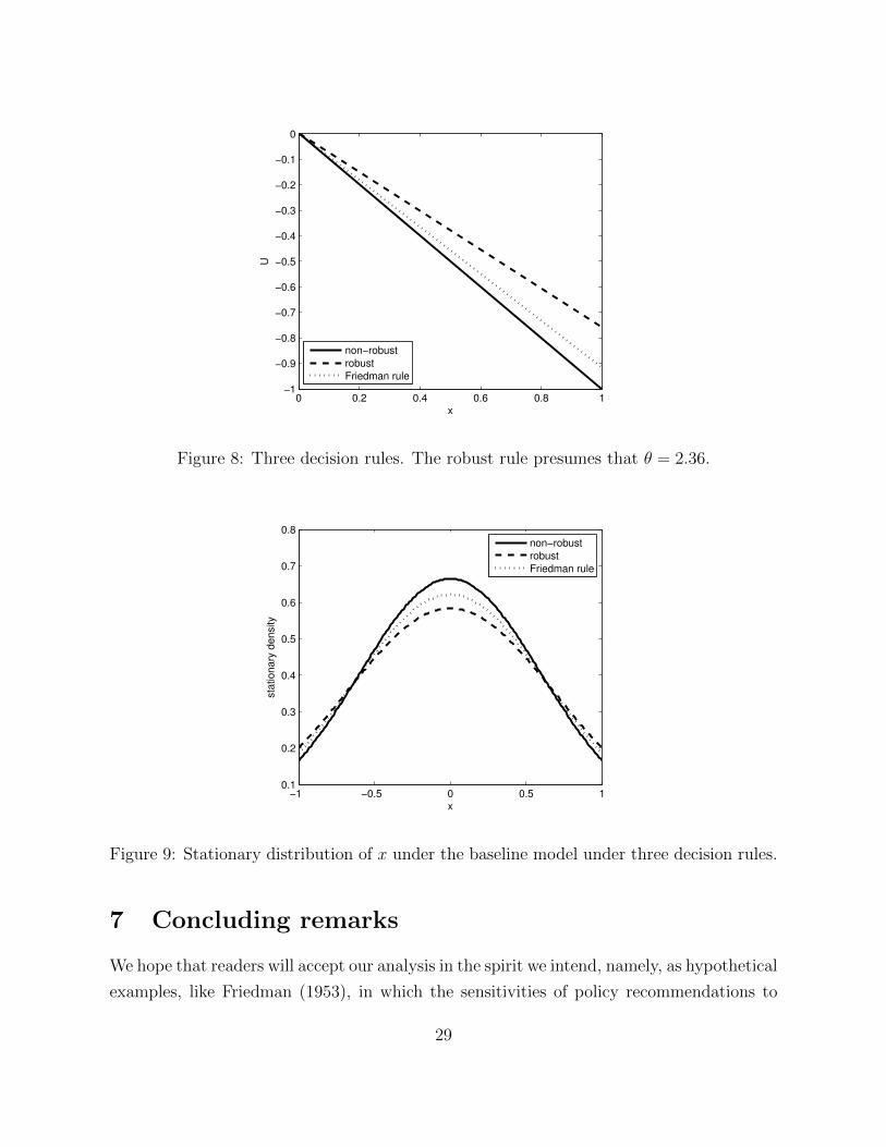
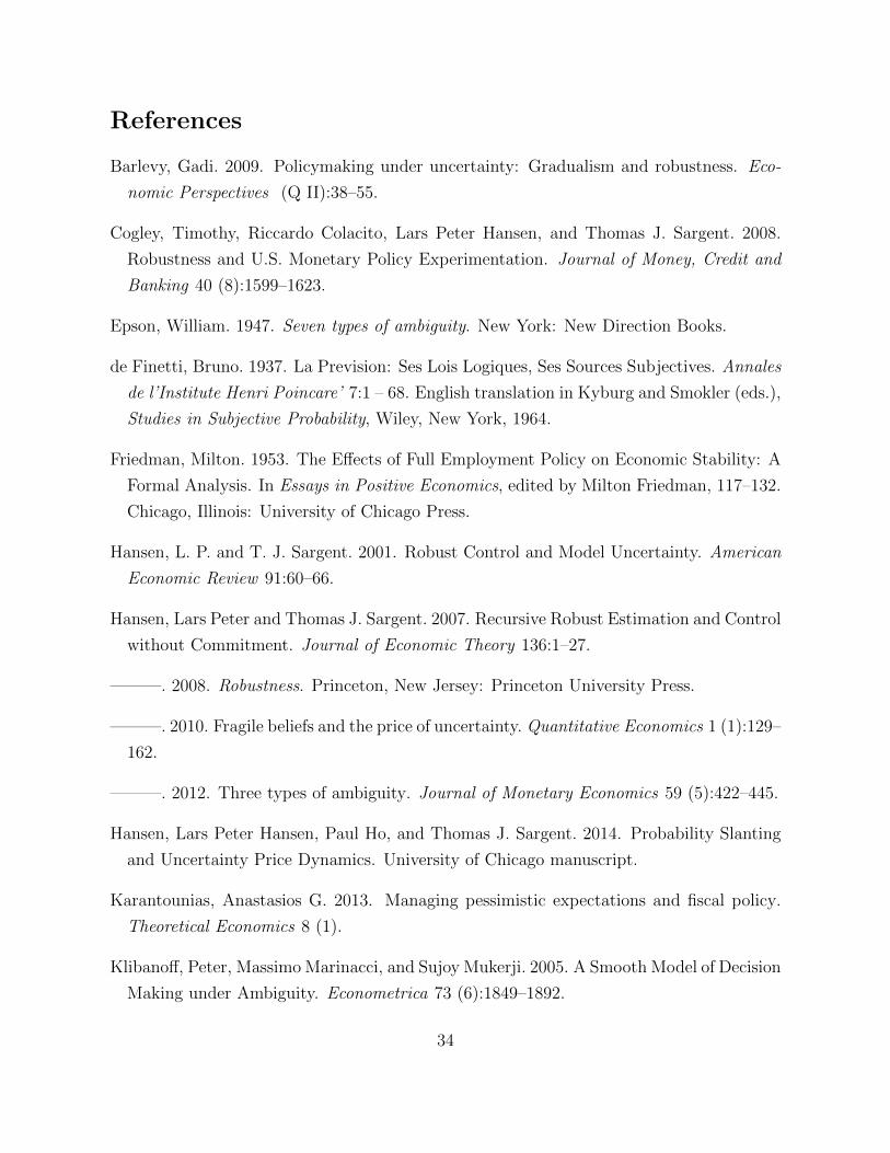
6.4 A Numerical Example
Consider the following numerical example:
Xt+1 = .8Xt + Ut + .6Wt+1,
which implies that the stationary distribution of Xt is a standard normal. Let h33 = .09
and the other the entries of the H matrix equal to zee
As suggested in our robustness analysis, we can impose a constraint on adjusted entropy
by computing θ to solve
maxθV (x; θ),
subject to the appropriate discounted intertemporal version of our adjusted relative en-
tropy constraint. Figure 6 shows an example of V (x, θ). The maximizing value of θ is
approximately 2.36 when the initial value x = 1. There is in fact very little dependence on
x as is shown in Figure 7. Figure 8 compares three decision rules. Figure 9 plots stationary
distributions under three decision rules under the baseline model (1).
27

1 2 3 4 5 6 7 8 9 10−26
−25.5
−25
−24.5
−24
−23.5
−23
−22.5
−22
θ
V
Figure 6: Value V (x, θ) as a function of θ.
0 0.5 1 1.5 20
0.5
1
1.5
2
2.5
3
x
θ
Figure 7: θ as a function of x.
28
0 0.2 0.4 0.6 0.8 1−1
−0.9
−0.8
−0.7
−0.6
−0.5
−0.4
−0.3
−0.2
−0.1
0
x
U
non−robust
robust
Friedman rule
Figure 8: Three decision rules. The robust rule presumes that θ = 2.36.
−1 −0.5 0 0.5 10.1
0.2
0.3
0.4
0.5
0.6
0.7
0.8
x
sta
tio
na
ry d
en
sity
non−robust
robust
Friedman rule
Figure 9: Stationary distribution of x under the baseline model under three decision rules.
7 Concluding remarks
We hope that readers will accept our analysis in the spirit we intend, namely, as hypothetical
examples, like Friedman (1953), in which the sensitivities of policy recommendations to
29

details of a model’s stochastic structure can be examined.18 Friedman’s finding that caution
due to model specification doubts translates into “doing less” as measured by a response
coefficient in a decision rule linking an action u to a state x depends on the structure
of the baseline model that he assumed. Even within single-agent decision problems like
Friedman’s but ones with different structures than Friedman’s, we know other examples in
which “being cautious” translates into “doing more now and picking up the pieces later.”
(For example, see Sargent (1999), Tetlow and von zur Muehlen (2001), Cogley et al. (2008),
and Barlevy (2009)). So the “do-less” flavor of some of our results should be taken with
grains of salt.
In more modern macreconomic models than Friedman’s, it is essential that there are
multiple agents. Refining rational expectations by imputing specification doubts to agents
inside or outside a model opens interesting channels of caution beyond those appearing
in the present paper. A model builder faces choices about to whom to impute model
specification doubts (e.g., the model builder himself or people inside the model) and also
what those doubts are about. Early work in multi-agent settings appears in Hansen and
Sargent (2012, 2008, ch. 15) and Karantounias (2013).
18For example, the “no-increase in caution” finding of section 5 depends on our having set up the objectivefunction to make it a “targetting problem”.
30

A Analysis of a two-period example (by David Evans
and Paul Ho)
This appendix analyses a two-period example designed to shed light on the shape of the
robust policy functions presented in the infinite horizon section 4 model of a Bayesian
decision maker who does not trust the prior distribution (5).
We take as given a continuation value function V (xt+1) = −12x2. With α = 0, V in
section 4 becomes
V (x, β, u) = −1
2(κx+ βu)2.
The T 2 operator from section 4 becomes
[T 2V ](x, u) = −θ log
[E exp
(−exp(−δ)
θV (x, β, u)|x, u
)]= −θ log
{1√2πσ
∫ ∞−∞
exp
(e−δ
2θ(κx+ βu)2
)exp
(−(β − µ)2
2σ2
)dβ
}. (35)
The integrand can be combined into
exp
[−1
2
(β2
(1
σ2− u2e−δ
θ
)− 2β
(uκxe−δ
θ+
µ
σ2
)+µ2
σ2− κ2x2e−δ
θ
)].
This integral exists only if1
σ2− u2e−δ
θ> 0,
which immediately implies an upper bound on the control u:
|u| ≤
√θ
σ2 exp−δ.
After several lines of algebra (checked with python code), the integrand in (35) can be
written as the following product:
1√2πσ
exp
(−1
2
[µ2
σ2− κx2e−δ
θ− (θµ+ uκxe−δσ2)2
σ2θ(θ − u2e−δσ2)
])exp
−(β − θµ+uκxe−δσ2
θ−u2e−δσ2
)22 σ2θθ−u2e−δσ2
31

The term on the left is independent of β and so can be pulled outside the integral, while
the infinite integral of the term on the right is easily computed to be√
2πσ√
θθ−u2e−δσ2 .
Plugging this into equation (35), we obtain
[T 2V ](x, u) =1
2
[µ2θ
σ2− κx2e−δ − (θµ+ uκxe−δσ2)2
σ2(θ − u2e−δσ2)− log
(θ
θ − u2e−δσ2
)]. (36)
We have verified this equation numerically using python code.
Remark A.1. The worst-case distribution of βt is
N(θµ+ uκxe−δσ2
θ − u2e−δσ2,
σ2θ
θ − u2e−δσ2
)The first-order condition for the maximization of the right side of equation (36) with
respect to u is
∂[T 2V ]
∂u=
1
2
[−2(θµ+ uκxe−δσ2)κxe−δσ2
σ2(θ − u2e−δσ2)− 2(θµ+ uκxe−δσ2)2ue−δσ2
σ2(θ − u2e−δσ2)2− θθ − u
2e−δσ2
θ
2θue−δσ2
(θ − u2e−δσ2)2
]=
−1
(θ − u2e−δσ2)2[(θµ+ uκxe−δσ2)κxe−δ(θ − u2e−δσ2)
+ (θµ+ uκxe−δσ2)2ue−δ + θue−δσ2(θ − u2e−δσ2)]
(37)
Thus, the optimal policy |u| ≤√
θσ2e−δ
solves the following cubic equation
(θµ+uκxe−δσ2)κxe−δ(θ−u2e−δσ2)+(θµ+uκxe−δσ2)2ue−δ+θue−δσ2(θ−u2e−δσ2) = 0 (38)
Note that as x→ ±∞, equation (38) will be dominated by the term
uκ2x2e−δσ2(θ − u2e−δσ2) + (κe−δσ2)2u3e−δx2
= ux2[κ2e−δσ2(θ − u2e−δσ2) + (κe−δσ2)2u2e−δ
].
The term in the brackets is positive and bounded away from zero, implying that u→ 0 as
x→ ±∞.
Remark A.2. Because it is always possible to set u = 0 and thereby remove the conse-
quences of risk and uncertainty about β, there is no lower bound on θ ∈ (0,∞).
32

B Computations (by David Evans)
We approximating the value function V (x) in the Bellman equation (15) over an interval
[−x, x] with cubic splines. For realizations of x outside [−x, x] a quadratic function that best
fit the value function at the interpolation points was assumed. To apply the three mappings
underlying (15), we used Gauss-Hermite quadrature to integrate over the Gaussian random
variables. The program iterated over the bellman equations until a desired tolerance was
achieved. Robustness checks were performed over the number of integration nodes for the
quadrature operation.
33
References
Barlevy, Gadi. 2009. Policymaking under uncertainty: Gradualism and robustness. Eco-
nomic Perspectives (Q II):38–55.
Cogley, Timothy, Riccardo Colacito, Lars Peter Hansen, and Thomas J. Sargent. 2008.
Robustness and U.S. Monetary Policy Experimentation. Journal of Money, Credit and
Banking 40 (8):1599–1623.
Epson, William. 1947. Seven types of ambiguity. New York: New Direction Books.
de Finetti, Bruno. 1937. La Prevision: Ses Lois Logiques, Ses Sources Subjectives. Annales
de l’Institute Henri Poincare’ 7:1 – 68. English translation in Kyburg and Smokler (eds.),
Studies in Subjective Probability, Wiley, New York, 1964.
Friedman, Milton. 1953. The Effects of Full Employment Policy on Economic Stability: A
Formal Analysis. In Essays in Positive Economics, edited by Milton Friedman, 117–132.
Chicago, Illinois: University of Chicago Press.
Hansen, L. P. and T. J. Sargent. 2001. Robust Control and Model Uncertainty. American
Economic Review 91:60–66.
Hansen, Lars Peter and Thomas J. Sargent. 2007. Recursive Robust Estimation and Control
without Commitment. Journal of Economic Theory 136:1–27.
———. 2008. Robustness. Princeton, New Jersey: Princeton University Press.
———. 2010. Fragile beliefs and the price of uncertainty. Quantitative Economics 1 (1):129–
162.
———. 2012. Three types of ambiguity. Journal of Monetary Economics 59 (5):422–445.
Hansen, Lars Peter Hansen, Paul Ho, and Thomas J. Sargent. 2014. Probability Slanting
and Uncertainty Price Dynamics. University of Chicago manuscript.
Karantounias, Anastasios G. 2013. Managing pessimistic expectations and fiscal policy.
Theoretical Economics 8 (1).
Klibanoff, Peter, Massimo Marinacci, and Sujoy Mukerji. 2005. A Smooth Model of Decision
Making under Ambiguity. Econometrica 73 (6):1849–1892.
34

———. 2009. Recursive smooth ambiguity preferences. Journal of Economic Theory
144 (3):930–976.
Kreps, David M. 1988. Notes on the Theory of Choice. Underground Classics in Economics.
Westview Press.
Petersen, I. R., M. R. James, and P. Dupuis. 2000. Minimax Optimal Control of Stochastic
Uncertain Systems with Relative Entropy Constraints. IEEE Transactions on Automatic
Control 45:398–412.
Prescott, Edward C. 1972. The Multi-Period Control Problem Under Uncertainty. Econo-
metrica 40 (6):1043–58.
Sargent, Thomas J. 1999. Dicsussion of “Policy Rules for Open Economies” by Laurence
Ball. In Monetary Policy Rules, edited by John Taylor, 144–154. Chicago, Illinois: Uni-
versity of Chicago Press.
Tetlow, Robert J. and Peter von zur Muehlen. 2001. Robust monetary policy with mis-
specified models: Does model uncertainty always call for attenuated policy? Journal of
Economic Dynamics and Control 25 (6-7):911–949.
Wald, Abraham. 1939. Contributions to the Theory of Statistical Estimation and Testing
Hypotheses. The Annals of Mathematical Statistics 10 (4):pp. 299–326.
35