Foundations of swarm roboticchemical plume tracing froma fluid dynamics perspective

Diana F. SpearsSwarmotics, LLC, Laramie, Wyoming, USA

David R. ThayerPhysics and Astronomy Department, University of Wyoming, Laramie,

Wyoming, USA, and

Dimitri V. ZarzhitskyComputer Science Department, University of Wyoming,

Laramie, Wyoming, USA

Abstract

Purpose – In light of the current international concerns with security and terrorism, interest isincreasing on the topic of using robot swarms to locate the source of chemical hazards. The purpose ofthis paper is to place this task, called chemical plume tracing (CPT), in the context of fluid dynamics.

Design/methodology/approach – This paper provides a foundation for CPT based on the physicsof fluid dynamics. The theoretical approach is founded upon source localization using the divergencetheorem of vector calculus, and the fundamental underlying notion of the divergence of the chemicalmass flux. A CPT algorithm called fluxotaxis is presented that follows the gradient of this mass flux tolocate a chemical source emitter.

Findings – Theoretical results are presented confirming that fluxotaxis will guide a robot swarmtoward chemical sources, and away from misleading chemical sinks. Complementary empirical resultsdemonstrate that in simulation, a swarm of fluxotaxis-guided mobile robots rapidly converges on asource emitter despite obstacles, realistic vehicle constraints, and flow regimes ranging from laminarto turbulent. Fluxotaxis outperforms the two leading competitors, and the theoretical results areconfirmed experimentally. Furthermore, initial experiments on real robots show promise for CPT inrelatively uncontrolled indoor environments.

Practical implications – A physics-based approach is shown to be a viable alternative to existingmainly biomimetic approaches to CPT. It has the advantage of being analyzable using standardphysics analysis methods.

Originality/value – The fluxotaxis algorithm for CPT is shown to be “correct” in the sense that it isguaranteed to point toward a true source emitter and not be fooled by fluid sinks. It is experimentally(in simulation), and in one case also theoretically, shown to be superior to its leading competitors atfinding a source emitter in a wide variety of challenging realistic environments.

Keywords Robotics, Chemical technology, Fluid dynamics

Paper type Research paper

The current issue and full text archive of this journal is available at

www.emeraldinsight.com/1756-378X.htm

This paper was partially supported by the National Science Foundation, Grant No. NSF44288.

Foundationsof swarm robotic

chemical plume

745

Received 6 February 2009Revised 22 July 2009

Accepted 15 August 2009

International Journal of IntelligentComputing and Cybernetics

Vol. 2 No. 4, 2009pp. 745-785

q Emerald Group Publishing Limited1756-378X

DOI 10.1108/17563780911005863

1. IntroductionThe chemical plume tracing (CPT) task is a search and localization problem, in whichone must find locations where potentially harmful substances are being released intothe environment. The ability to quickly locate chemical sources is an integralcomponent of numerous manufacturing and military activities. In light of the currentinternational concerns with security and the possibility of a chemical terrorist attack,many private and government agencies, including the Japan Defense Agency, the USDepartment of Homeland Security, the US Defense Advanced Research ProjectsAgency (DARPA), the Danish Environmental Protection Agency, the UK HealthProtection Agency (HPA), and local emergency response agencies throughout theworld have expressed interest in updating techniques used to track hazardous plumes,and improving the search strategies used to locate an active chemical toxin emitterBoard on Atmospheric Sciences and Climate (2003), Shinoda (2003), and ChemicalHazards and Poisons Division, HPA (2006). As a result, there is a growing interestamong both researchers and engineers in designing robot-based approaches to solvethis problem.

There are two main motivations for this paper. The first is to cast CPT as a fluiddynamics problem. The second is to clarify the advantages of using a fluid-based CPTapproach for solving a fluid-based problem. When the Environmental Fluid Mechanicsjournal published a special issue on the topic of CPT in Cowen (2002), the papers in thatissue were groundbreaking in the sense that they laid an initial foundation for the field.Like the majority of prior and current CPT strategies, the strategies presented in thespecial issue were based on observations of living organisms, e.g. insects, land animals,aerial, and aquatic creatures. In other words, the CPT strategies outlined in that specialissue were biomimetic, i.e. they were designed to mimic biological systems. Theobjective of this paper is to establish a theoretical foundation for an alternative type ofstrategy – one that is physicomimetic, or physics-based, i.e. it is designed to mimic theway in which physical particles such as molecules behave. Swarm robotic systemsbased on physicomimetics, also called artificial physics, use virtual forces to maintain adesired inter-robot distance (Spears and Gordon, 1999). Using such virtual forces, therobots can achieve lattice formations, which are ideal for computing derivatives. Virtualforces then attract the lattice toward desirable regions in the environment, such aschemical density maxima. Our new physicomimetic approach to multi-robot CPTexploits fundamental principles of fluid dynamics to drive a swarm lattice to a chemicalsource emitter.

What motivated us to explore a physics-based alternative? The chief difficulty withbiomimetic algorithms is that in order to mimic natural biological strategies with robots,sophisticated sensors are needed. However, despite recent advances in manufacturingtechniques, state-of-the-art chemical sensors remain crude and inefficient compared totheir biological counterparts. In short, it is difficult to achieve optimal or near-optimalperformance in artificial CPT systems by relying on mimicry of biological systemsalone. For example, Crimaldi et al. (2002) analyzed crustaceans’ “antennae” sensorarrays, also called “olfactory appendages,” and found that an antennae structure withmultiplicity and mobility improves an organism’s CPT performance. But we can surpassthis with cooperating mobile robots. In particular, the inherent flexibility afforded by themultiplicity and mobility of a swarm (large group) of robots far exceeds that of a singleorganism’s antennae.

IJICC2,4

746

Throughout this paper, we will emphasize the advantage of this swarm-basedphysicomimetic CPT approach, in which autonomous robots employ strategies derivedfrom many years of advanced human study on the topic of fluid dynamics. We are fullyaware of the limitations on the ability to predict and model advanced turbulent flowdynamics and chemical transport due to the non-linear and stochastic nature of theseprocesses. However, as we demonstrate in this paper, we already have enoughunderstanding and mathematical expertise at our disposal to design a complete roboticsystem for locating chemical sources based on the physical cues extracted from localfluid observations. Furthermore, our ability to handle both laminar and turbulent flowregimes (the latter containing filaments or packets of chemical that are not fully diffused)with our CPT approach has been demonstrated experimentally (Zarzhitsky and Spears,2005; Zarzhitsky et al., 2004a, b, c, 2005; Spears D. et al., 2005) for a variety of differentexperiments.

If physicomimetic (i.e. physics-based) strategies based on the fundamentals of fluiddynamics can be shown to complement existing search techniques, then autonomousland, marine, and micro-air vehicles can use physicomimetic or hybrid (combined)physicomimetic-biomimetic CPT algorithms to improve their performance. Here, weexplore the theoretical underpinnings of plume tracing and source localizationstrategies that are derived from a fundamental understanding of fluids. Since theemphasis of this paper is on the fluid dynamics foundation of CPT, we examine themost fluid-based approach to CPT, called fluxotaxis, in much greater depth thanthe other CPT strategies. Theoretical results presented in this paper show thatfluxotaxis is competitive with or outperforms the two most popular CPT strategies,under realistic conditions. Furthermore, we have implemented and extensively testedour fluxotaxis approach in simulation and demonstrated its superiority over other CPTalgorithms under a wide variety of realistic flow conditions (Zarzhitsky, 2008).Performance metrics included precision and consistency of finding the emitter, andswarm scalability.

Section 2 presents an overview of the CPT problem and its practical importance.The relevance of this work to the design of intelligent robotic systems is examined inSection 3, where we place the fluid analyses in the context of multi-robot CPT;an implementation and experiments with CPT on real hardware robots is discussed.Then, Sections 4 and 5 provide the necessary background for understanding how ourCPT approach is a natural application of fluid physics. Section 6 details the specifics ofthe CPT task and its subtasks, and then Sections 7 and 8 provide an overview ofrelated work on two of these subtasks. In Section 8, we describe the fluxotaxistechnique as the first robotic CPT approach based on an application of fluid dynamicsin the context of chemical plumes and emitters. Since fluxotaxis is the mostfluid-oriented of all the CPT approaches, it is further theoretically analyzed in theremainder of the paper. Section 9 contains a formal analysis of the fluxotaxis approach,and Section 10 compares fluxotaxis with the most widely employed chemotaxisstrategy from the perspective of fluid dynamics. Our analytical results provide aquantitative measure of how effective these strategies are in predicting the direction ofthe source chemical emitter. Section 11 provides experimental evidence in simulationof the practical value of the theory. Finally, Section 12 presents conclusions andfuture work.

Foundationsof swarm robotic

chemical plume

747

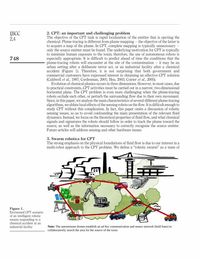
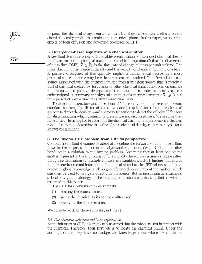
2. CPT: an important and challenging problemThe objective of the CPT task is rapid localization of the emitter that is ejecting thechemical. Plume tracing is different from plume mapping – the objective of the latter isto acquire a map of the plume. In CPT, complete mapping is typically unnecessary –only the source emitter must be found. The underlying motivation for CPT is typicallyto minimize human exposure to the toxin; therefore, the use of autonomous robots isespecially appropriate. It is difficult to predict ahead of time the conditions that theplume-tracing robots will encounter at the site of the contamination – it may be anurban setting after a deliberate terror act, or an industrial facility after a chemicalaccident (Figure 1). Therefore, it is not surprising that both government andcommercial customers have expressed interest in obtaining an effective CPT solution(Caldwell et al., 1997; Cordesman, 2001; Hsu, 2003; Coirier et al., 2005).

Evolution of chemical plumes occurs in three dimensions. However, in most cases, dueto practical constraints, CPT activities must be carried out in a narrow, two-dimensionalhorizontal plane. The CPT problem is even more challenging when the plume-tracingrobots occlude each other, or perturb the surrounding flow due to their own movement.Since, in this paper, we analyze the main characteristics of several different plume-tracingalgorithms, we ablate local effects of the sensing robots on the flow. It is difficult enough tostudy CPT without this complication. In fact, this paper omits a discussion of roboticsensing issues, so as to avoid confounding the main presentation of the relevant fluiddynamics. Instead, we focus on the theoretical properties of fluid flow, and what chemicalsignals and signatures the robots should follow in order to track the plume toward thesource, as well as the information necessary to correctly recognize the source emitter.Future articles will address sensing and other hardware issues.

3. Swarm robotics for CPTThe strong emphasis on the physical foundations of fluid flow is due to our interest in amulti-robot approach to the CPT problem. We define a “robotic swarm” as a team of

Figure 1.Envisioned CPT scenarioof an intelligent roboticswarm responding to achemical accident at anindustrial facility Note: The autonomous drones establish an ad hoc communication and sensor network (bold lines) to

collaboratively search the area for the source of the toxin

IJICC2,4

748

mobile autonomous vehicles that cooperatively solve a common problem. The swarmsize and type may vary anywhere from a few simple, identical robots to thousands ofdifferent hardware platforms, including ground-based, aquatic (autonomoussurface/underwater vehicles), or aerial (unmanned air vehicles). In our swarmdesign, each mobile robot serves as a dynamic node in a distributed sensor andcomputation network, so that the swarm as a whole functions as an adaptive sensinggrid, constantly sharing various fluid measurements between adjacent vehicles.Weissburg et al. (2002) provide convincing evidence for the CPT performanceadvantage of sampling the plume at multiple, spatially separated locationssimultaneously. Spears et al. (2004) have confirmed this finding in numerousexperiments on a group of autonomous CPT robots.

We want to emphasize the importance and value of consistent adherence to thephysicomimetic design philosophy for each component of the system. In order tounderstand the benefits of implementing our physics-based approach, consider thefollowing three functional aspects of a swarm of physicomimetic robots. The mostimportant facet is of course, the robots’ cooperative behavior, which we achieve byemulating real-world physics in the on-board control software, using virtual “social”forces for maintaining desired inter-robot distances. In other words, robots that usephysicomimetics act as particles, analogous to molecules within a solid, liquid, or gas, sothat the whole swarm mimics properties of a real-world physical substance. Thisenables us to use standard physics analysis techniques to estimate the swarm’sperformance prior to its deployment (Spears W. et al., 2005). The resulting ability toanalytically predict both the short- and long-term behavior of physicomimetic systemsoffers tremendous advantages for fielding reliable robotic collectives.

At the same time, we can also view the swarm of intelligent robots as a distributed,adaptive computational fluid dynamics grid or mesh. This functionality is the directconsequence of structured swarm formations, because adjacent vehicles can share theirlocal fluid observations, thus boosting the effective resolution of their on-board flowsensors. Our physicomimetics-driven swarm system is a viable and compellingalternative to static in situ sensing grids.

Lastly, observe that the on-going exchange of sensor measurements between vehicleshelps the robots to process sensor data simultaneously from many different locations.Therefore, we can employ the swarm as a distributed, mobile computer capable ofdynamic configuration and run-time load balancing. This unique feature ofphysicomimetics allows our robotic systems to address the growing interest indistributed computing with a flexible, low maintenance solution, ideally suited fordeployment in areas lacking the necessary communication and data-processinginfrastructure. Furthermore, the swarm performs fully distributed computation in thesense that each robot in the swarm shares sensor values with its immediate neighborsonly, and decides where to move next based only on that strictly local information. Thereis no explicit collaboration between distant swarm members. Aggregate swarmbehavior emerges implicitly, without any global coordination.

Since our present goal is to test the swarm on the plume tracing task, this paperdefines some of the fluid dynamics equations and mathematical approximationtechniques that intelligent robots can employ to improve their emitter localizationperformance. We also consider requirements for implementing and analyzinga physics-based swarm-oriented chemical source localization algorithm called

Foundationsof swarm robotic

chemical plume

749

“fluxotaxis,” which we derived from theoretical analyses of fluid-driven chemicaltransport effects. The fluxotaxis-driven swarm moves like a fluid through the plume, andthe robots’ on-board software, which is based on fluid theory described here, analyzeschemical emissions and the ambient fluid in order to perform effective chemical sourcelocalization. In other words, our CPT approach is physicomimetic in two differentrespects. First, the robots use physicomimetics to stay in fluid-like (bendable) latticeformations as they trace the plume in search of the chemical emitter. Second, whenexecuting the fluxotaxis CPT algorithm, the robots use physicomimetic methods foranalyzing the fluid flow and rely on fluid dynamics principles to estimate the location ofthe chemical emitter. The remainder of this paper will focus on the latter physicomimeticcapabilities of the swarm, i.e. we will describe the CPT algorithms used by the robots,instead of the virtual physics that organizes the robots into formations.

We have demonstrated in a robot-faithful simulation, with swarms of hundreds ofrobots, that our physicomimetic CPT theory is directly applicable to a distributed swarmrobotic paradigm. Fluid velocity and chemical concentration are measured independentlyby each robot and, as we stated above, the collected sensor data are communicated betweenneighboring vehicles in order to calculate (partial) derivatives. Derivative calculations areperformed by the robots using the numerical finite-difference method of second-orderaccurate central differences (Zarzhitsky, 2008). Note that this short-range sharing ofinformation between robots is sufficient for calculating local navigation gradients, so thereis never a need for a “global broadcast” of these values. In other words, implementation ofthe theory we present here requires no leaders or central controllers or global information,which in turn increases the system’s overall robustness, while lowering its cost.

Zarzhitsky et al. (2005) show that fluxotaxis is a practical algorithm that can beimplemented on a swarm of inexpensive, distributed, autonomous, collaboratingrobots. They describe how the basic fluxotaxis algorithm is tested, refined andevaluated in comprehensive software simulations, and introduce swarm-specific CPTperformance evaluation metrics. The simulation work is of interest because it solvesthe multi-robot cooperation and coordination problem by using physicomimetic designbased on virtual (artificial) social forces (Spears et al., 2004), as described above. Thisallows the robots to self-organize in an emergent (i.e. without explicit programming)fashion into a dynamic sensor lattice as they navigate toward the chemical emitter.Spears D. et al. (2005) show that this swarm-based distributed computer is well-suitedfor performing fluid-dynamic computations.

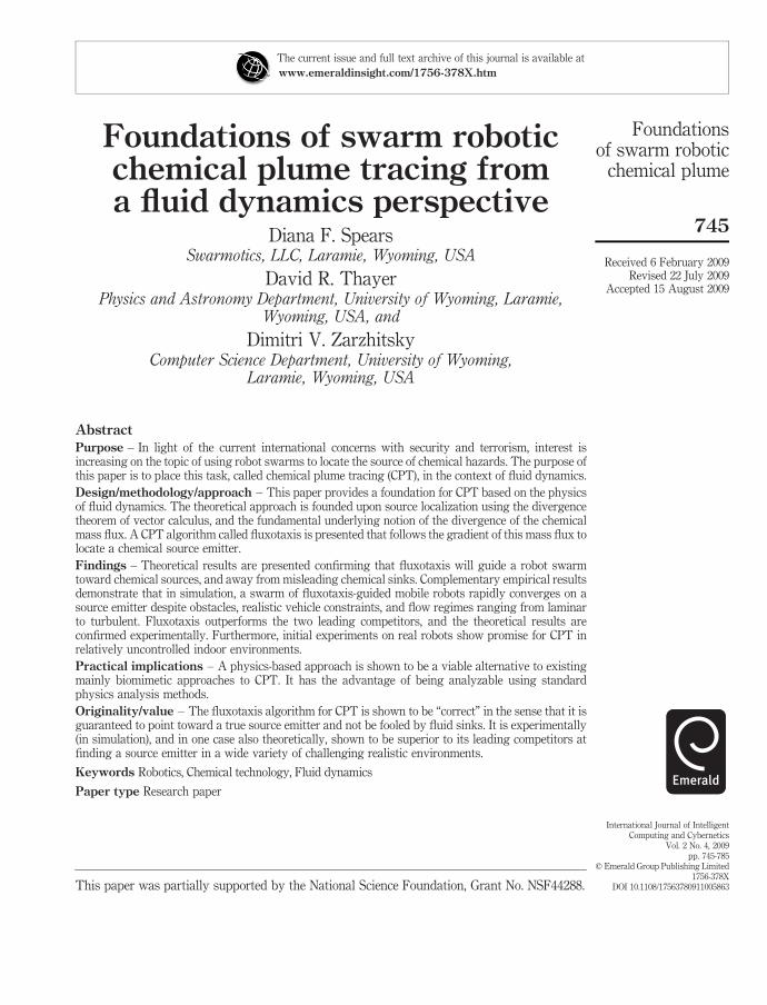
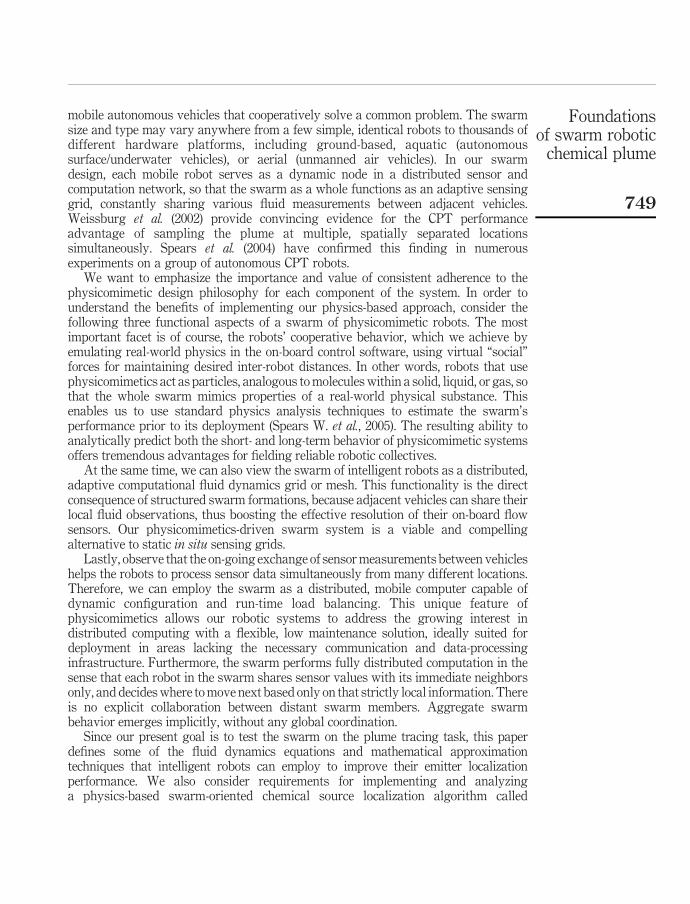
As part of our comprehensive research effort, we applied one of the CPT algorithmsdiscussed in this paper (chemotaxis, which follows the chemical density gradient) to ourmobile robot prototype, and then ran tests using laboratory-scale ethanol vapor plumeconfigurations. Figure 2, adapted from Spears et al. (2006), shows our distributed CPT

Figure 2.A laboratory-scale CPTscenario, in whichminiature robotic vehiclessuccessfully find a sourceof ethanol vapor(top-right)

IJICC2,4

750

implementation, featuring three robots equipped with a miniature metal-oxide volatileorganic compound sensor, in addition to an inexpensive 16-bit microcontroller that isable to process a limited amount of sensor data and make autonomous navigationdecisions. Each robot has the ability to localize other robots using an RF-sonarcombination for trilateration, and to communicate sensor readings using low-power,short-range radio transceivers. The distributed, decentralized nature of our designendows it with several desirable properties, including self-organization, self-repair, andefficient resource utilization (Spears et al., 2004). These desirable properties are achieveddespite sensor noise and latency, non-holonomic drives, limited velocity and accelerationcapabilities, localization noise, and even in the presence of occasional hardware failures.Furthermore, the environment was surprisingly uncontrolled during the experiments –people walked into and out of the room in which the experiments were being conducted,windows leaked airflow into the room, and the robots unexpectedly shoved the emitteron occasion. Despite these hindrances, as well as exceptionally stringent metrics forsuccess, our success rate is on par with that of more controlled experiments found in theliterature. Spears et al. (2006) describe indoor laboratory experiments demonstrating thesuccess of CPT (chemotaxis) on the real robots.

Research is currently in progress to identify and integrate anemometers with therobot platforms because in the near future we plan to implement anemotaxis andfluxotaxis on the robots as well. Anemotaxis is a strategy for traveling upwind.(Note that even though for simplicity of presentation we sometimes use gas-specificterms such as “upwind” or “airflow,” the CPT algorithms apply to aquaticenvironments as well. In other words, anemotaxis vehicles travel upstream when inwater.) Indoor and outdoor experiments will be performed to compare the three CPTstrategies under a wide variety of real-world conditions.

4. CPT as an application of fluid dynamicsWe have found that the foundation of effective CPT algorithms can be naturally andeffectively built upon the fundamentals of fluid dynamics. This section shows therelationship between fluid physics and CPT. Note that the term “fluid” refers to bothgaseous and liquid states of matter. The theoretical results presented in this paper areapplicable to both gases and liquids. Therefore, our findings are applicable to thedesign of ground, marine, and aerial autonomous vehicles.

A physical description of a fluid medium consists of density, velocity, specific weightand gravity, viscosity, temperature, pressure, and so on. Here, due to their relevance andimportance to the goals of CPT, we focus on the scalar density r, which has the units ofmass per unit volume, and the vector velocity ~V. Since our focus is on CPT, we use theterm “density” and its symbol r to denote the concentration of the chemical being traced,rather than the density of the carrier fluid. For simplicity of presentation, unless statedotherwise, this paper assumes that the ambient fluids are compressible because inreality all materials are to some extent compressible. Furthermore, relative to aplume-tracing vehicle in motion, the distinction between the velocities of the fluid-bornechemical and that of the chemical-bearing fluid is often well below the sensor resolutionthreshold. In our model of the chemical plume, we assume that the chemical and ambientfluid velocities are identical.

Consider an infinitesimal fluid element moving within the plume. The velocity of thiselement can be represented as the vector ~V ¼ uiþ vjþ wk, where i, j, and k are the

Foundationsof swarm robotic

chemical plume

751

orthonormal basis vectors along the x-, y-, and z-axes in R3, i.e. ~V ¼, u; v;w .. Notethat u ¼ uðx; y; z; tÞ, v ¼ vðx; y; z; tÞ, w ¼ wðx; y; z; tÞ, and t denotes time. Since chemicalflow is typically unsteady, › ~V=›t – 0 in the general case. The density and othercharacteristics of the fluid, i.e. the “flow-field variables,” are likewise functions of spaceand time.

Sensor measurements of these flow-field variables are collected by the robots. Inparticular, it is assumed that a swarm of mobile vehicles equipped with chemical andfluid flow sensors can sample the plume to determine the current state of thecontamination, and then use their on-board computers to collaboratively decide the mosteffective direction in which to move next. The calculations and collaborative decisionscan be effectively based upon the physical rules that govern the flow of fluids, as we willdemonstrate shortly.

The three governing equations of computational fluid dynamics for modeling fluidflow are the continuity, momentum, and energy equations. The continuity equationensures that mass is conserved, the momentum equation captures Newton’s second law~F ¼ m~a, and the energy equation enforces energy conservation. Each equation can beexpressed in at least four different forms, depending on one’s perspective with respect tothe fluid:

(1) a finite control volume fixed in space with the fluid moving through it;

(2) a finite control volume moving with the fluid;

(3) an infinitesimal fluid element fixed in space with the fluid moving through it; or

(4) an infinitesimal fluid element moving with the fluid (Anderson, 1995).

Selecting the third perspective, which is the most intuitive formulation for CPT, wewrite the conservation of mass equation as:

›r

›t¼ 2~7 · ðr ~VÞ: ð1Þ

One can see that this equation expresses the physical fact that the time rate of decreaseof mass inside the differential element (left-hand side) must equal the net mass fluxflow (right-hand side) out of the element. Since we focus on numerical, rather thananalytical, solutions to the fluid equations for use by computationally restricted robots,we retain the fundamental forms of these equations, rather than adopt a fullNavier-Stokes formulation.

To model fluid flow, the equations are solved using numerical methods. In the caseof perspective (3), the method of finite differences is often employed. For the CPTproblem, a distinction must be made between the forward solution and the inversesolution. The former consists of a simulation that models the chemical flow, and thelatter requires tracing within the fluid to find the source emitter, i.e. the latter is CPT.For the purposes of developing and testing new CPT approaches in simulation, theforward solution is required. Once the CPT algorithm has been refined influid-dynamic simulations, then the forward solution is no longer necessary, sincethe robots are tested with real laboratory-scale chemical plumes (Figure 2). However,note that the inverse solution (i.e. the CPT algorithm) is required for both thesimulation and laboratory testing.

A numerical model of the forward solution for a given fluid provides data at discretepoints in space, i.e. at “grid points.” Abstractly, one can see a relationship between grid

IJICC2,4

752

points and robots in a swarm. This abstract correspondence motivates our view of aswarm of robots as a distributed computer that jointly senses the flow-field variables,shares them with their immediate neighbors, and then decides in which direction tomove in order to locate the chemical emitter, thereby performing embodied computation.This relationship will be exploited, as relevant, in the remainder of the paper.

Consider one very important variable to measure in the context of CPT – thedivergence of the velocity of the fluid (and therefore of the chemical). Note that as afluid flows, any element within that fluid has invariant mass, but its volume canchange. The divergence of the velocity, ~7 · ~V, is the time rate of change of the volume ofa moving fluid element, per unit volume. The divergence is the rate at which a fluidexpands, or diverges, from an infinitesimally small region. A local vector field withpositive divergence expands, and is called a source; a vector field with negativedivergence contracts, and is called a sink. The magnitude of the divergence vector,j~7 · ~Vj, is a measure of the rate of expansion or contraction. A vector field with zerodivergence, when measured over the entire velocity vector field, is called solenoidal.The definition of solenoidal implies fluid incompressibility. This can be understood byconsidering the ~7 · ~V ¼ 0 constraint on the conservation of mass (1), whereð›=›t þ ~V · ~7Þr ¼ 0, so that the total time derivative is zero, dr=dt ¼ 0, whichindicates that the fluid density is constant when viewed along the trajectory of amoving fluid element. Hence, compressible fluid flow with sources and sinks is notonly realistic, but is also desirable – because the sources and sinks can facilitate localnavigation in the absence of global landmarks (Decuyper and Keymeulen, 1991). Mostimportantly, a mathematical source (in terms of divergence) that remains a source overtime (i.e. it is not transient) indicates a chemical emitter, whose identification is the keyto successful CPT. This will be discussed in-depth below, because it is the reason whyCPT is naturally considered as an application of fluid dynamics.

First, however, we need to broaden the notion of divergence to include the chemicaldensity, in addition to the wind velocity. The key notion we seek is that of chemicalmass flux, or mass flux for short. The mass flux is the product of the (chemical) densityand the velocity, i.e. r ~V. Informally, this is “the stuff spewing out of the chemicalemitter.” An astute reader will now infer that what would be of great interest for CPT isthe divergence of the mass flux, which is, in mathematical notation in 3D:

~7 · ðr ~VÞ ¼ ~V · ~7rþ r~7 · ~V ¼ u›r

›xþ r

›u

›xþ v

›r

›yþ r

›v

›yþ w

›r

›zþ r

›w

›z: ð2Þ

The divergence of the mass flux is the time rate of change of mass per unit volume lostat any spatial position. If this divergence is positive, it indicates a source of mass flux;if negative, it indicates a sink of mass flux. Sustained (over a period of time) positivedivergence of chemical mass flux implies chemical spewing outward from a chemicalsource emitter, as opposed to a transient source.

To conclude this section, consider two modes of fluid transport: diffusion andadvection. Diffusion dominates in an indoor setting where the air is relatively stagnant,e.g. when the windows are closed and there is little disturbance in the room. It alsodominates at smaller spatial scales, e.g. insects tend to be more sensitive to diffusiveeffects than larger animals (Crimaldi et al., 2002). In the absence of air flow, diffusion ofchemical mass away from a chemical source will result in a Gaussian density profile.Advection is a more macroscopic phenomenon than diffusion. Both are at work to

Foundationsof swarm robotic

chemical plume

753

disperse the chemical away from an emitter, but they have different effects on thechemical density profile that makes up a chemical plume. In this paper, we examineeffects of both diffusion and advection processes on CPT.

5. Divergence-based signature of a chemical emitterA key fluid dynamics concept that enables identification of a source of chemical flow isthe divergence of the chemical mass flux. Recall from equation (2) that the divergenceof mass flux (DMF), ~7 · ðr ~VÞ, is the time rate of change of mass per unit volume. Themass flux combines chemical density and the velocity of chemical flow into one term.A positive divergence of this quantity implies a mathematical source. In a morepractical sense, a source may be either transient or sustained. To differentiate a truesource associated with the chemical emitter from a transient source that is merely apuff of chemical created by turbulence or other chemical distribution phenomena, werequire sustained positive divergence of the mass flux in order to identify a clearemitter signal. In summary, the physical signature of a chemical emitter is ~7 · ðr ~VÞ . 0for a period of t experimentally determined time units.

To detect this signature and to perform CPT, the only additional sensors (beyondstandard sensors, like IR for obstacle avoidance) required for robots are chemicalsensors to detect the density r and anemometer sensors to detect the velocity ~V. Sensorsfor discriminating which chemical is present are not discussed here. We assume theyhave already been applied to determine the chemical class. This paper focuses instead onrobots that need to determine the value of r, i.e. chemical density rather than type, for aknown contaminant.

6. The inverse CPT problem from a fluids perspectiveComputational fluid dynamics is adept at modeling the forward solution of real fluidflows for the purposes of theoretical analysis and engineering design. CPT, on the otherhand, seeks a solution to the inverse problem. Assuming that at least one sourceemitter is present in the environment (for simplicity, herein we assume a single emitter,though generalization to multiple emitters is straightforward)[1], finding that sourcerequires environmental information. In an ideal situation, the CPT robots would haveaccess to global knowledge, such as geo-referenced coordinates of the emitter, whichcan then be used to navigate directly to the source. But in most realistic situations,a local navigation strategy is the best that the robots can do, and that is what isassumed in this paper.

The CPT task consists of three subtasks:

(1) detecting the toxic chemical;

(2) tracing the chemical to its source emitter; and

(3) identifying the source emitter.

We consider each of these subtasks, in turn[2].

6.1 The chemical detection subtask: explorationAt the initiation of CPT, it is frequently assumed that the robots are not in contact withthe chemical. Therefore, their first job is to locate the chemical plume. Under theassumption that they have no background knowledge about where the emitter is,

IJICC2,4

754

the best they can do is to engage in an undirected exploratory search. In the literature,this search typically takes the form of a zigzag or spiral pattern (Hayes et al., 2001;Russell et al., 2000). It is called casting because the robots are essentially casting aboutthe environment, looking for a detectable (i.e. above sensor threshold) amount of thechemical. Casting strategies are often motivated by observation of biological creatures,such as insects, birds, or crustaceans (Grasso and Atema, 2002).

The chemical detection subtask is not described further in this paper. Although it isa very important part of CPT, the focus of this paper is on CPT from a fluid dynamicsperspective, and casting strategies are not fluids-based.

6.2 The plume tracing subtask: following local signalsThe objective of the plume tracing subtask is to follow clues, which are typically localif robots are used, to increase one’s proximity to the source emitter. We have identifiedfive major classes of algorithms for this subtask:

(1) Heuristic strategies.

(2) Chemotaxis strategies. Usually, these algorithms follow chemical gradients.

(3) Infotaxis strategies. There is a wide variety of algorithms in this class. A popularversion follows the frequency of chemical puffs (i.e. filamentary structures)which typically increases in the vicinity of the emitter.

(4) Anemotaxis strategies. These algorithms move the robots upwind.

(5) Hybrid strategies. The more modern tracing approaches combine both chemicaland upwind strategies.

More details, along with references, will be provided in Section 8. First, however, weelaborate a bit on the motivation for chemotaxis, infotaxis, and anemotaxis.

The chemotaxis strategy of chemical gradient following is motivated primarily bythe chemical diffusion process that is responsible for some of the dispersion of thechemical from the emitter. Recall that diffusion creates a Gaussian chemical profile,i.e. the chemical density is highest near the emitter and it is reduced exponentially asdistance from the emitter increases. In particular, the diffusive Gaussian chemicaldensity profile can be modeled using the density diffusion equation, which is alsosimply called the diffusion equation. In its simplest 1D form, this equation is:

›r

›t¼ D

›2r

›x 2:

This equation describes the time evolution of the density of chemical particles, rðx; tÞ,as a function of position, x, and time, t. It is particularly useful to consider a temporalinitial condition (t ¼ 0) when all the chemical is contained at the origin (x ¼ 0),represented as the Dirac delta function particle source, i.e. rðx; 0Þ ¼ NdðxÞ, where N isthe total number of chemical filaments. dðxÞ is the delta function, which has the value 0everywhere except at x ¼ 0, where its value is infinitely large and the total spatialintegral is one. D is the diffusion coefficient, which is proportional to the square of themean free path, lmfp, divided by the collision time, tcoll, of particles in the fluid, that is,D/ l2

mfp=tcoll. The mean free path is the average distance traveled by particles in thefluid before they collide. The collision time is the average time between such collisions.

The solution to the 1D density diffusion equation, with a delta function initialcondition, is the Gaussian evolution function:

Foundationsof swarm robotic

chemical plume

755

rðx; tÞ ¼Nffiffiffiffiffiffiffiffiffiffiffi

4pDtp e2ðx2xoÞ

2=4Dt;

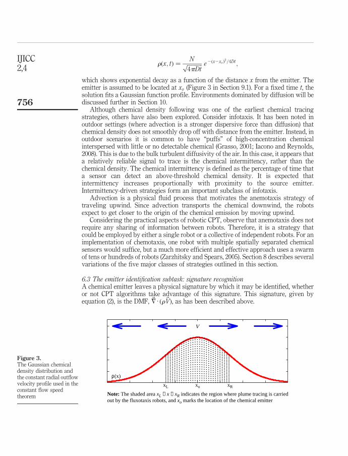
which shows exponential decay as a function of the distance x from the emitter. Theemitter is assumed to be located at xo (Figure 3 in Section 9.1). For a fixed time t, thesolution fits a Gaussian function profile. Environments dominated by diffusion will bediscussed further in Section 10.

Although chemical density following was one of the earliest chemical tracingstrategies, others have also been explored. Consider infotaxis. It has been noted inoutdoor settings (where advection is a stronger dispersive force than diffusion) thatchemical density does not smoothly drop off with distance from the emitter. Instead, inoutdoor scenarios it is common to have “puffs” of high-concentration chemicalinterspersed with little or no detectable chemical (Grasso, 2001; Iacono and Reynolds,2008). This is due to the bulk turbulent diffusivity of the air. In this case, it appears thata relatively reliable signal to trace is the chemical intermittency, rather than thechemical density. The chemical intermittency is defined as the percentage of time thata sensor can detect an above-threshold chemical density. It is expected thatintermittency increases proportionally with proximity to the source emitter.Intermittency-driven strategies form an important subclass of infotaxis.

Advection is a physical fluid process that motivates the anemotaxis strategy oftraveling upwind. Since advection transports the chemical downwind, the robotsexpect to get closer to the origin of the chemical emission by moving upwind.

Considering the practical aspects of robotic CPT, observe that anemotaxis does notrequire any sharing of information between robots. Therefore, it is a strategy thatcould be employed by either a single robot or a collective of independent robots. For animplementation of chemotaxis, one robot with multiple spatially separated chemicalsensors would suffice, but a much more efficient and effective approach uses a swarmof tens or hundreds of robots (Zarzhitsky and Spears, 2005). Section 8 describes severalvariations of the five major classes of strategies outlined in this section.

6.3 The emitter identification subtask: signature recognitionA chemical emitter leaves a physical signature by which it may be identified, whetheror not CPT algorithms take advantage of this signature. This signature, given byequation (2), is the DMF, ~7 · ðr ~VÞ, as has been described above.

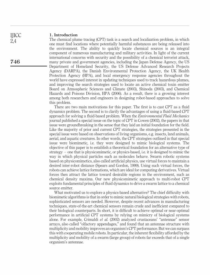
Figure 3.The Gaussian chemicaldensity distribution andthe constant radial outflowvelocity profile used in theconstant flow speedtheorem

V

ρ(x)

xL xo xR

Note: The shaded area xL ≤ x ≤ xR indicates the region where plume tracing is carriedout by the fluxotaxis robots, and xo marks the location of the chemical emitter

IJICC2,4

756

Of course, the type of emitter will also have an effect on the character of its signature.There are continuous emitters, as well as single-puff emitters, and regularly andirregularly pulsing emitters. In this paper, we will address single-puff and continuousemitters – because real-world CPT problems typically contain a source that is acombination of these basic emission modes. Nevertheless, note that these are justexamples; our theory is general and is not restricted to these two types of emitters. Thesize, shape, orientation, and height of an emitter can also affect the plumecharacteristics. The theoretical results in this paper are deliberately general, but couldbe parametrized as needed to model particular emitter geometries and configurations.

7. The major strategies for the emitter identification subtask7.1 Heuristic strategiesOne of the most popular heuristic approaches to emitter identification is a comparison ofthe chemical density at different heights (Cowen, 2002). The work of Grasso and Atema(2002) assumes that the emitter is low to the ground; they declare discovery of the emitterwhen the bottom sensor on their robot reports chemical detection for 90 percent of thesampling period. This percentage was empirically determined with experiments. On theother hand, Buscemi et al. (1994) determine that the emitter has been reached whenthe chemical sensors become saturated. Note that these heuristic approaches are prone toa high rate of false alarms (i.e. erroneously labeling sustained regions of high chemicalconcentration, such as areas next to walls or obstacles, as the source).

7.2 Machine learning strategiesAs an alternative to heuristic techniques, the emitter identification subtask can beperformed using machine learning approaches. For example, Lilienthal et al. (2004)treat this as a classification problem and use neural networks and support vectormachines to learn to identify a chemical source. The advantage of this approach is thatafter training, they were able to achieve approximately 85 percent of the maximum hitrate. The disadvantage is that it requires a training phase, which makes the perhapsunrealistic assumption that the emitter type on which training occurs will be similar tothe emitter type to be encountered during the actual CPT mission.

The approach adopted by Weissburg et al. (2002) could also be considered amachine learning approach. Their system is trained on characteristic emitter andnon-emitter chemical patterns; it is then able to detect the emitter more accurately.

7.3 Emitter identification with fluxotaxisRecall from Section 5 that the physical signature of a chemical emitter is ~7 · ðr ~VÞ . 0 for aperiod of t (experimentally determined) time units. How could this signature be identifiedby a team of robots trying to solve the emitter identification problem? Fluxotaxis employsthe divergence theorem of vector calculus (Hughes-Hallett et al., 1998):Z

Wo

~7 · ðr ~VÞdW ¼

IAo

ðr ~VÞ · ndA: ð3Þ

Simply put, the left side of this equation is a volume integral of the DMF, while the rightside of the equation is the surrounding surface area integral of the mass flux in theoutward normal direction. This equation, where Wo is the control volume, Ao is thebounding surface of the volume, and n is a unit vector pointed as an outward normal to

Foundationsof swarm robotic

chemical plume

757

the surface of the volume, allows us to formally define the intuitive notion that a controlvolume containing a source will have a positive mass flux divergence, whereas a controlvolume containing a sink will have a negative mass flux divergence. This result canbe used as the basic criterion for theoretically identifying a chemical emitter, which is atrue mathematical source under this definition. In particular, equation (3) shows that if therobots encircle a suspected emitter, and the total mass flux exiting the circle of robotsconsistently exceeds some small, empirically determined threshold for a given amount oftime, then the robots are known to surround a true chemical emitter. Our fluxotaxisalgorithm uses this theoretical criterion. To the best of our knowledge, previous criteriafor emitter identification are purely heuristic (Cowen, 2002). Fluxotaxis is the first with afirm theoretical basis.

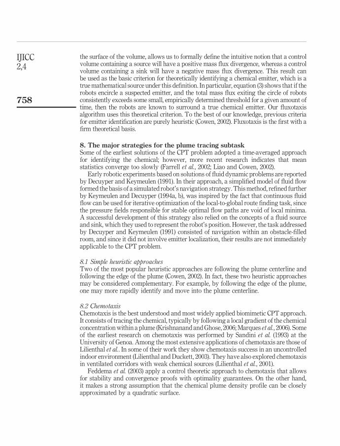
8. The major strategies for the plume tracing subtaskSome of the earliest solutions of the CPT problem adopted a time-averaged approachfor identifying the chemical; however, more recent research indicates that meanstatistics converge too slowly (Farrell et al., 2002; Liao and Cowen, 2002).

Early robotic experiments based on solutions of fluid dynamic problems are reportedby Decuyper and Keymeulen (1991). In their approach, a simplified model of fluid flowformed the basis of a simulated robot’s navigation strategy. This method, refined furtherby Keymeulen and Decuyper (1994a, b), was inspired by the fact that continuous fluidflow can be used for iterative optimization of the local-to-global route finding task, sincethe pressure fields responsible for stable optimal flow paths are void of local minima.A successful development of this strategy also relied on the concepts of a fluid sourceand sink, which they used to represent the robot’s position. However, the task addressedby Decuyper and Keymeulen (1991) consisted of navigation within an obstacle-filledroom, and since it did not involve emitter localization, their results are not immediatelyapplicable to the CPT problem.

8.1 Simple heuristic approachesTwo of the most popular heuristic approaches are following the plume centerline andfollowing the edge of the plume (Cowen, 2002). In fact, these two heuristic approachesmay be considered complementary. For example, by following the edge of the plume,one may more rapidly identify and move into the plume centerline.

8.2 ChemotaxisChemotaxis is the best understood and most widely applied biomimetic CPT approach.It consists of tracing the chemical, typically by following a local gradient of the chemicalconcentration within a plume (Krishnanand and Ghose, 2006; Marques et al., 2006). Someof the earliest research on chemotaxis was performed by Sandini et al. (1993) at theUniversity of Genoa. Among the most extensive applications of chemotaxis are those ofLilienthal et al.. In some of their work they show chemotaxis success in an uncontrolledindoor environment (Lilienthal and Duckett, 2003). They have also explored chemotaxisin ventilated corridors with weak chemical sources (Lilienthal et al., 2001).

Feddema et al. (2003) apply a control theoretic approach to chemotaxis that allowsfor stability and convergence proofs with optimality guarantees. On the other hand,it makes a strong assumption that the chemical plume density profile can be closelyapproximated by a quadratic surface.

IJICC2,4

758

While chemotaxis is very simple to perform, it frequently leads to locations of highconcentration in the plume that are not the real source, e.g. a corner of a room (Song andChen, 2006). Cui et al. (2004) investigated an approach to solving this problem by usinga swarm majority vote, along with a communication and routing protocol fordistributing information to all members of a robotic collective. However, that is astrong requirement, and Cui et al. also make an even stronger assumption that eachrobot in the collective has a map of the environment.

In addition to the local maxima problem of chemotaxis, we show in Section 10 that achemotaxis search strategy can fail near the emitter’s location, due to the fact that for atypical, time-varying Gaussian distribution profile, the chemical density gradient goesto zero near the distribution’s peak.

8.3 InfotaxisThere are different varieties of infotaxis. One, which we call intermittency infotaxis, issimilar to chemotaxis because it considers only the chemical density and disregards theambient wind velocity. On the other hand, it is different from chemotaxis because itmeasures the chemical intermittency (i.e. the “puff” frequency), rather than densitygradients, to determine source proximity. Liao and Cowen (2002) demonstrate theadvantages of intermittency infotaxis over alternative approaches. Related tointermittency is the notion of coherency. Kikas et al. (2001) measure coherency usinga correlation analysis of temporal concentration fluctuations across a sensor array.

Justus et al. (2002) explore not only intermittency, but also the burst length, where“burst” is another name for a puff or filament. The burst length is found to be afiner-scale measure of source proximity than intermittency. In particular, frequentshort bursts and few long bursts both increase the intermittency. The intermittency ishigh near a chemical source, but it may also be high in other regions of the plume.Burst length enables discrimination of such cases.

A second type of infotaxis focuses on information theory and entropy. Vergassolaet al. (2007) have developed a strategy that locally maximizes the expected rate ofinformation gain, in an information theoretic sense. Actually, their approach is aBayesian and information theoretic variant of intermittency infotaxis. Anotherprobability-driven approach to infotaxis is the maximum likelihood approach ofBalkovsky and Shraiman (2002). They focus on carrier wind velocity, and maximize theconditional probability PðsourcejsequenceofobservationsÞ. Jeremic and Nehorai (1998)also use a maximum likelihood approach, but they use it for tuning parameters. Theseparameter values are learned for the purpose of instantiating a sensor model that takesinto account chemical measurements, signal bias and Gaussian noise.

Parunak and Brueckner (2001) conduct analysis of the self-organization property inmulti-robot systems from the standpoint of entropy and the second law ofthermodynamics. They develop an analogy between entropy and information disorder,and show how understanding and control of system entropy can be used to organize amulti-robot system. They illustrate the idea by solving a robot coordination problemwith the use of simulated randomly diffusing pheromones.

8.4 AnemotaxisAnother common approach, usually called “anemotaxis” but sometimes alternativelycalled odor gated rheotaxis, has been proposed for the CPT task. An anemotaxis-driven

Foundationsof swarm robotic

chemical plume

759

robot focuses on the advection portion of the flow. It measures the direction of thefluid’s velocity and navigates “upstream” within the plume. Hayes et al. (2001) havedone seminal work in this area. Grasso and Atema (2002) combine anemotaxis withcasting, so that the robots alternate moving upstream and cross-stream in the wind.The simulation results of Iacono and Reynolds (2008) show that the effectiveness ofanemotaxis improves with increased wind speed. More complex wind-driven strategiesmay be found in Kazadi et al. (2000). They have successfully explored a form ofanemotaxis that combines wind velocity information with passive resistive polymersensors and strategic robot placement which enables effective anemotaxis. Ishida et al.(2006) gain performance improvements by coupling anemotaxis with visioncapabilities.

One of the biggest advantages of anemotaxis is that it can be performed successfullywith either a single robot, or with a group of independent robots. The same also holds forinfotaxis. However, Grasso and Atema (2002) have found that two spatially separatedwind sensors outperform a single wind sensor. Although anemotaxis can be a veryeffective strategy for some problems, its limitation is that it can lead to a wind source thatis not the chemical emitter.

8.5 Heuristic hybridsRecently, there has been an increasing trend toward the development of hybrid CPTstrategies that combine chemotaxis with some form of anemotaxis. For example,Ishida et al. (2001) use a simple hybrid strategy that consists of applying anemotaxiswhen the chemical density r is high, and otherwise applying chemotaxis.

Russell et al. (2000) employ a more complex hybrid approach to CPT for finding thesource of a chemical emission in a maze. Their single CPT robot employs a heuristicalgorithm for traveling upwind, following the chemical and avoiding obstacles.

More unusual hybrids are the approaches adopted by Lytridis et al. (2006), Marqueset al. (2006). They combine chemotaxis with a biased random walk, and discover thatthis hybrid outperforms its components.

8.6 The fluxotaxis hybridFluxotaxis is the most fluid-based of all the strategies, and therefore the remainder ofthis section focuses on fluxotaxis. Recall the definition of the divergence of the massflux from equation (2). This divergence is the hallmark signature of a chemical sourceemitter. A logical conclusion is that following its gradient will take the robots closer tothe source. That is the essence of our fluxotaxis strategy, i.e. to follow the gradient ofthe divergence of mass flux, abbreviated

������!

GDMF , where the gradient is the direction ofsteepest increase. The mathematical formula for the

������!

GDMF in 3D is:

~7 ~7 · ðr ~VÞh i

¼ ~7 u›r

›xþ r

›u

›xþ v

›r

›yþ r

›v

›yþ w

›r

›zþ r

›w

›z

� �:

������!

GDMF combines information about both velocity and chemical density, in a mannermotivated by the theory of fluid dynamics. Mathematically, the DMF can besubdivided into two terms:

~7 · ðr ~VÞ ¼ rð~7 · ~VÞ þ ~V · ð~7rÞ: ð4Þ

Therefore, the������!

GDMF is a gradient ~7 of the sum of two terms:

IJICC2,4

760

(1) rð~7 · ~VÞ, which is the density times the divergence of the velocity field; and

(2) ~V · ð~7rÞ, which is the flow velocity field in the direction of the density gradient.

When the chemical flow is divergent, the first term takes precedence in directing therobots, and it is analogous to anemotaxis. When the fluid velocity is constant, or theflow is stagnant, then ~7 · ~V is zero and the second term is the only relevant term.This second term is the flow velocity in the direction of the density gradient, and is

analogous to chemotaxis. What is important here is that������!

GDMF theoretically combineschemotaxis and anemotaxis, and the relevant term is activated automatically basedon the environment. No deliberate strategy selection or switching mechanism is

required –������!

GDMF automatically becomes whatever it is supposed to be in anenvironmentally driven manner.

Next, consider the relationship between the emitter signature and������!

GDMF as anavigation strategy to locate the source emitter. In particular, suppose we apply������!

GDMF as an enclosure fluxotaxis algorithm. In other words, assume that there is arobot lattice consisting of hundreds of robots surrounding the emitter, thus creating afull sensing grid. Also, assume that the chemical source within the control volume, Wo,contains a total amount of chemical, Q, at time t so that when the source emitter ejectsthe chemical (in a chemical puff or continuous fashion), the time rate of change of thetotal chemical is negative, dQ=dt , 0. Then we have a formal guarantee regarding������!

GDMF as an enclosure navigation strategy. In particular, a key diagnostic of thechemical plume emitter location is when we have

HAoðr ~VÞ · ndA . 0, where Ao is the

surface area of the volumetric region Wo that the robots are known to surround. IfQ ¼

RWo

rdW is the total chemical in the control volume Wo, then from theconservation of mass equation (1), integrated over the control volume, while using thedivergence theorem equation (3), the time rate of change of the total chemical:

dQ

dt¼ 2

IAo

ðr ~VÞ · ndA;

is indeed found to be negative, i.e. dQ=dt , 0, which is indicative of a source. In otherwords, a robot lattice surrounding the emitter can locate it by going opposite to thedirection of flux outflow. In this case, we have a theoretical guarantee that the

enclosure������!

GDMF strategy will allow the robot lattice to home in on the source emitter.In order to backtrack where the source of the chemical plume originated, it is

reasonable to look in the direction of the������!

GDMF vector.At this point, it is important to merge the global and local perspectives being

maintained simultaneously above and in the remainder of this paper. From the globalperspective, the reality (from both a fluids and a fluxotaxis perspective) is that we aredealing with control volumes for which we calculate the surface integral of the massflux. Under typical real-world transient fluid conditions, within volumes near thechemical emitter the flux inflow frequently does not equal the flux outflow. It takestime for the chemical mass to move away from the emitter prior to reaching steadystate (at which point there is no CPT signal for the robots to track). During thetransient period of fluid emission, there are numerous volumetric regions that mimic“sources” and “sinks,” sometimes far away from the emitter, where the chemicalaccumulates temporarily. In other words, the plume consists of a highly dynamic flow

Foundationsof swarm robotic

chemical plume

761

of chemical-laden fluid, which is moving unsteadily through the region aroundthe emitter. Typically, this implies that in a significantly large region containing achemical source, the surface area flux integral will be nonzero, thereby providing agradient signal for the robots to follow. By following the regions that behave likesources, fluxotaxis-driven robots quickly, and easily find the true source emitter. Innumerous computational fluid dynamics simulations we have found that ourgradient-following fluxotaxis algorithm quickly and reliably locates the source emitterusing these ambient chemical flux signals. Even in complex, simulated urbanenvironments filled with many large buildings and narrow passageways, we haveshown that fluxotaxis demonstrates rapid and reliable success, whereas the leadingalternative approaches typically flounder and fail (Agassounon et al., 2009).

The analogous local perspective is that of the������!

GDMF defined above. The������!

GDMF is anidealized, local concept that we use as a visualization tool to illustrate what fluxotaxis does.

With������!

GDMF we assume an infinitesimal analysis based on differential calculus thatreasonably approximates the global volumetric perspective. Although in reality we have afinite grid (both in simulation and with the robots), we can compute an approximate

solution by assuming that the������!

GDMF can be calculated at every point in space.

Mathematically, we are stating that ~7HAoðr ~VÞ · ndA

h ibecomes equivalent to ~7 ~7 · ðr ~VÞ

h iin the limit as we move from discrete grids to continuous space. The latter is the

������!

GDMF

formula. The advantage of adopting the local������!

GDMF perspective is that it simplifies our

analysis without loss of correctness. Using������!

GDMF we can clearly illustrate whyfluxotaxis-guided robots move in the correct direction toward the source emitter.

To conclude this section, we briefly mention some practical considerations forapplying fluxotaxis and other CPT methods. Any CPT strategy will only be valid inregions where the value of r and its gradients (if computed by the strategy) are abovesome minimally significant threshold. Below this minimum density (e.g. too far fromthe source emitter), all CPT algorithms will be poor predictors of the source location,and the robots should resort to casting. Fluxotaxis navigates best in the presence ofsources and sinks, which are common in realistic fluid flows, and it performs well in allother CPT fluid conditions in which we have tested it. It is robust in its avoidance ofsinks, and exceptionally precise in homing in on sources. Interestingly, we haveexperimentally determined that a local, neighbor-oriented, first-derivative

approximation of������!

GDMF works best for swarms of robots navigating in regions faraway from sources and sinks, with above-threshold levels of chemical. In such regions,the density may not be sufficiently far above the threshold for a second derivative to beuseful, and therefore a first-derivative approximation is more suitable. With thisversion of fluxotaxis, every robot calculates the component of mass flux, r ~V, in thedirection from each locally sensed neighbor to itself, and it moves in the direction in

which this scalar value is maximized. This swarm-oriented first-derivative������!

GDMFapproximation, which improves as the swarm size increases, is discussed at length byZarzhitsky (2008). We will not discuss it further in this paper because it is animplementation issue. Instead, this paper focuses exclusively on the precise,

second-derivative, original������!

GDMF formulation. Finally, for solenoidal regions inwhich the fluid is incompressible and the chemical density is invariant along velocitytrajectories, heuristic CPT approaches or casting must be used. When the chemical has

IJICC2,4

762

dissipated for a long time and a steady state has been reached, there will be nochemical derivative signal for any CPT strategy to follow.

9. A theoretical fluid-based analysis of fluxotaxisIn the previous section, we presented multiple strategies for the plume tracing subtaskof CPT. Most of these strategies are motivated by biological CPT systems, and thus donot use fluid dynamics principles for an emitter signature identification. The oneexception is the fluxotaxis strategy, which is derived fully from the fluid dynamicsproperties of chemical plumes. Since this paper is about CPT from a fluid dynamicsperspective, this section explores the physical underpinnings of fluxotaxis, and wefocus on the gradient of the divergence of the chemical mass flux – a fundamentalcomponent of the fluxotaxis algorithm.

In this section, we prove a sequence of theorems that elucidate the strengths of������!

GDMFas a local guide for finding the chemical emitter[3]. The assumptions may, at first blush,appear to be restrictive; however, they form the basis for some of the most realistic flowsituations to be encountered in environmental scenarios. Furthermore, there isno assumption about the robot lattice surrounding the emitter. All of these theoremsassume a shared coordinate system between neighboring robots[4]. The section assumesa single coordinate axis (1D) for simplicity of presentation – so that the reader can gainthe necessary insight and intuition into our approach. In other words, to explain why������!

GDMF is effective, we begin with a 1D tutorial perspective when presenting ourtheoretical results. Furthermore, for improved clarity, we focus on static “snapshots,” ormoments in time. However, we have verified the correctness of all results for thedynamic 2D and 3D cases. Section 9.4 summarizes the 3D version of this analysis.

Let us begin with a 1D environment, where the robot lattice consists of a linearformation of spatially separated robots. Each robot can detect the chemical density

r and the wind velocity ~V in its vicinity, and calculate the������!

GDMF via an exchange ofsensor data with its neighbors. The objective of this section is to present theorems

regarding whether the������!

GDMF vector calculated by the grid robots “points toward”(is predictive of) the source emitter, or “points away from” a sink, under three classicalenvironmental conditions:

(1) a constant flow speed;

(2) a chemical flow source; and

(3) a chemical flow sink.

Fluid compressibility is assumed for the source and sink results, but not for theconstant flow results.

The technique employed in these theorems and proofs is to select two points, Pemt

and P far, where two robots are stationed within the lattice, so that the former is closer tothe emitter, and the latter is farther from the emitter. At each time step, the robots share

their DMF values, calculate the������!

GDMF , and then move in the direction of the������!

GDMF

vector. If DMFemt . DMFfar then the������!

GDMF will predict the correct direction – towardthe chemical source. When dealing with sinks, on the other hand, two points Psnk andP far are identified and in this case the correct prediction occurs whenDMFsnk , DMFfar. In other words, the correct robot behavior is to avoid sinks.

Foundationsof swarm robotic

chemical plume

763

The two robots under consideration could be any pair of neighbors within the latticethat share their DMF values to determine the new direction in which to navigate.

9.1 1D GDMF and constant flow speedConstant flow speed theorem. Assume that the following conditions hold:

. The chemical plume has a Gaussian distribution rðxÞ ¼ ke2ðx2xoÞ2=Dx 2

, centeredat xo, where Dx is the density profile scale length.

. The lattice is positioned between xL and xR , where xL and xR are solutions to(Figure 3):

›2rðxÞ

›x 2¼ 0;

this implies that ›2rðxÞ=›x 2 , 0 in the region of interest. This is the regionwhere CPT can be effective.

. ~V is constant in magnitude throughout the flow, except right at the emitter (xo),and is an outward radial vector.

Without loss of generality, assume the existence of robots at points Pemt and P far, suchthat Pemt is closer to the emitter than P far. Then execution of one step of the fluxotaxisalgorithm implies that the robot lattice moves closer to the emitter, or equivalently:

u›r

›xþ r

›u

›x

� �far

, u›r

›xþ r

›u

›x

� �emt

: ð5Þ

Proof. The problem is symmetric with respect to the emitter’s location (xo); thus, it issufficient to prove the case where xL , P far , Pemt , xo. Since j ~Vj is constant,›u=›x ¼ 0, and equation (5) simplifies to:

u›r

›x

� �far

, u›r

›x

� �emt

:

Since u is a negative constant, the inequality can be simplified to:

›r

›x

� �far

.›r

›x

� �emt

:

Grouping like terms gives:

0 .›r

›x

� �emt

2›r

›x

� �far

:

This is true because, by Assumption 2:

0 .›2r

›x 2:

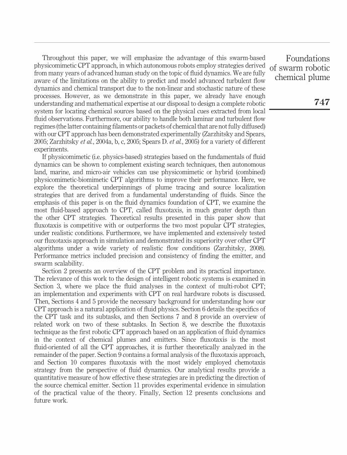
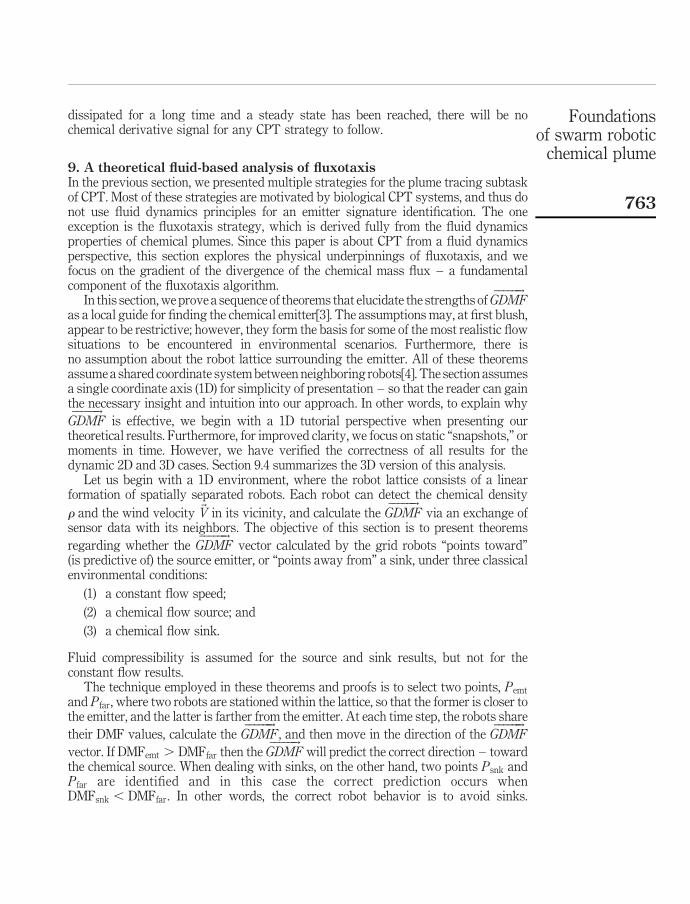
Results of a software simulation for this theorem are shown in Figure 4. In the figure,light-colored areas denote large values, and dark-colored areas correspond to smallvalues. The location of the chemical emitter is marked by the triangle symbol. Theinitial positions of two separate robot lattices are at the outer edges of the environment,

IJICC2,4

764

to the left and right of the emitter. During execution of the fluxotaxis algorithm, eachrobot (shown as a black box with a white £ in the middle) computes the DMF usingequation (2), with the partial derivatives replaced by the second-order accurate centraldifference approximation (Zarzhitsky, 2008). This value is recorded by the simulatorfor analysis purposes, and is displayed along with the final robot positions in thescreenshot. Observe that the resulting divergence “landscape” has a global peak thatcoincides with the location of the emitter, and does not have any local maxima thatcould trap or mislead the robots. There is a small gap in the computed divergence plotnear the emitter because the robots had terminated their search upon reaching theemitter. Each simulated robot (the black box) corresponds to one of the reference points(Pemt or P far) in the theorem’s proof and, just as in the theorem, there are two robots perlattice. In this simulation, both robot lattices correctly moved toward the emitter in thecenter. In the proof of the constant flow speed theorem, we only considered the casewhere the lattice was to the left of the emitter; however, a similar proof can be given forthe symmetric case, where the lattice starts out on the right side of the emitter, and thesimulation in Figure 4 shows that the algorithm works regardless of the initial positionof the robot lattice with respect to the position of the chemical source.

9.2 1D GDMF at a sourceSource theorem. The fluxotaxis

������!

GDMF will advance the robot lattice toward achemical source.

Proof. As before, assume a general Gaussian chemical plume distribution. Withoutloss of generality, assume the existence of two points Pemt and P far, such that Pemt iscloser to the source than P far (Figure 5). Two cases result, based on the orientation ofthe lattice coordinate axis.

Figure 4.Simulation results for the

constant flow speedtheorem

Chemical density (the highest density is in the middle, right at the emitter):

Fluid velocity (uniform radial split at the emitter):

Lattice-computed divergence of mass flux (the maximum is near the emitter):

Two-sided lattice trace (agents move inward, toward the emitter):

1 2 3 4 5 6 6 5 4 3 2 1

Notes: Individual robots are shown as black boxes with the white × in the middle, and thetime trace of the two independent robot lattices is shown with boxed numbers indicating thelocation of the lattice at a given time step. The theorem holds for any initial latticeconfiguration, and fluxotaxis successfully locates the chemical emitter

Foundationsof swarm robotic

chemical plume

765

Case I. assumes that the direction of the lattice coordinate axis is opposite to thedirection of the fluid flow, and thus:

(1) ›2u=›x 2 $ 0;

(2) ›u=›x . 0; thus 0 $ uemt . ufar;

(3) ›2r=›x 2 # 0; and

(4) ›r=›x . 0 and therefore remt . rfar:

We need to prove that the robot will move toward the source, or:

u›r

›xþ r

›u

›x

� �far

, u›r

›xþ r

›u

›x

� �emt

: ð6Þ

Assumptions 1 and 3 imply:

›u

›x

� �far

#›u

›x

� �emt

and›r

›x

� �far

$›r

›x

� �emt

:

Together, with Assumptions 2, 4, and algebraic rules, Case I holds. ACase II. is with the lattice coordinate axis in the same direction as the fluid flow, so

that both uemt and ufar are non-negative (Figure 5), and the previous assumptionsbecome:

(1) ›2u=›x 2 # 0;

(2) ›u=›x . 0; thus 0 # uemt , ufar;

(3) ›2r=›x 2 # 0; and

(4) ›r=›x , 0 and therefore remt . rfar:

The robot will turn around and move toward the source if equation (6) holds. FromAssumption 1, we conclude:

›u

›x

� �far

#›u

›x

� �emt

:

Similarly, Assumption 3 yields:›r

›x

� �far

#›r

›x

� �emt

:

Algebraic application of the remaining assumptions shows that equation (6) holds. ASoftware simulation of this theorem’s configuration for both cases is shown in

Figure 6. As before, two������!

GDMF-driven lattices (represented by black boxes marked withthe white £ symbol) begin at the outer edges of the simulated environment, and move in

Figure 5.Local coordinate axis ofthe CPT vehicles andemitter location in thesource theorem

PemtPfar

V

(a) Case I

PemtPfar

V

(b) Case II

IJICC2,4

766

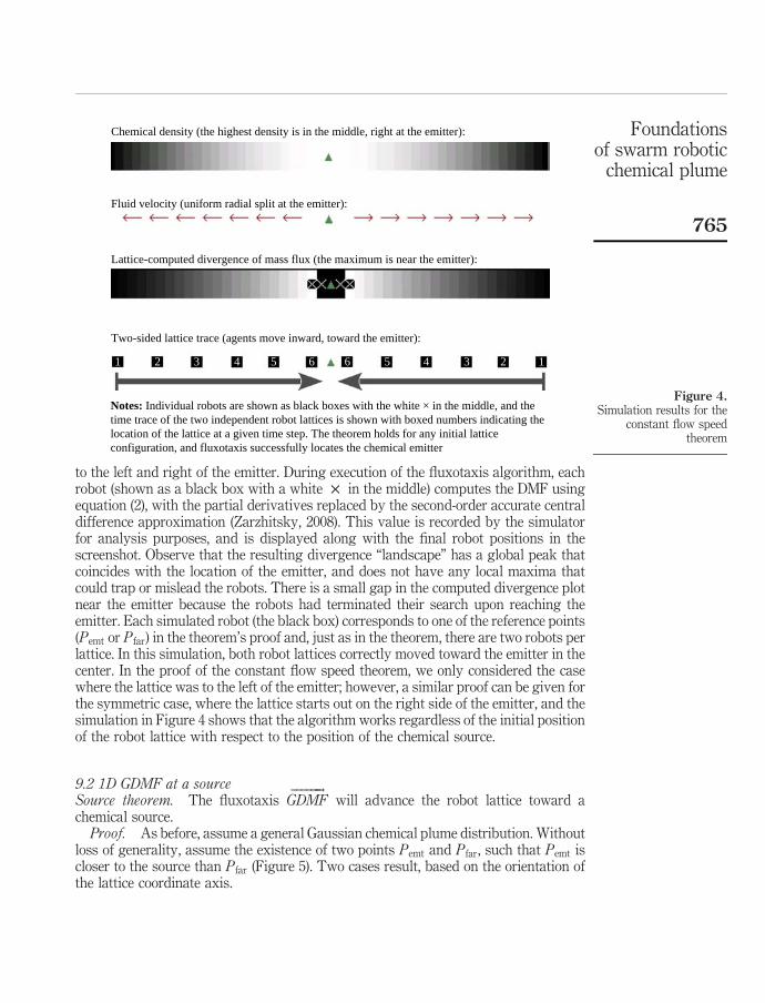
toward the emitter, denoted by the triangle in the center. The direction of motion isdetermined by the gradient of the DMF, which is computed locally by each robot using acentral difference approximation of the partial derivatives in equation (2), and as canbeen seen from the divergence plot, has the maximum value near the emitter’s location.Similar to the previous simulation, the divergence value right at the emitter is notcomputed by the lattice, since the search terminates as soon as the emitter is found. Twofluxotaxis lattices are shown in the screenshot, and as expected, both of themsuccessfully navigate toward the chemical source. As this figure illustrates, the initialposition of a lattice with respect to the emitter does not affect the robots’ ability tocorrectly localize the emitter. We should note here that in order to succeed, a robot latticemust discern between a transient versus a sustained source. An approach fordistinguishing between transient and sustained sources is outlined in Section 5.

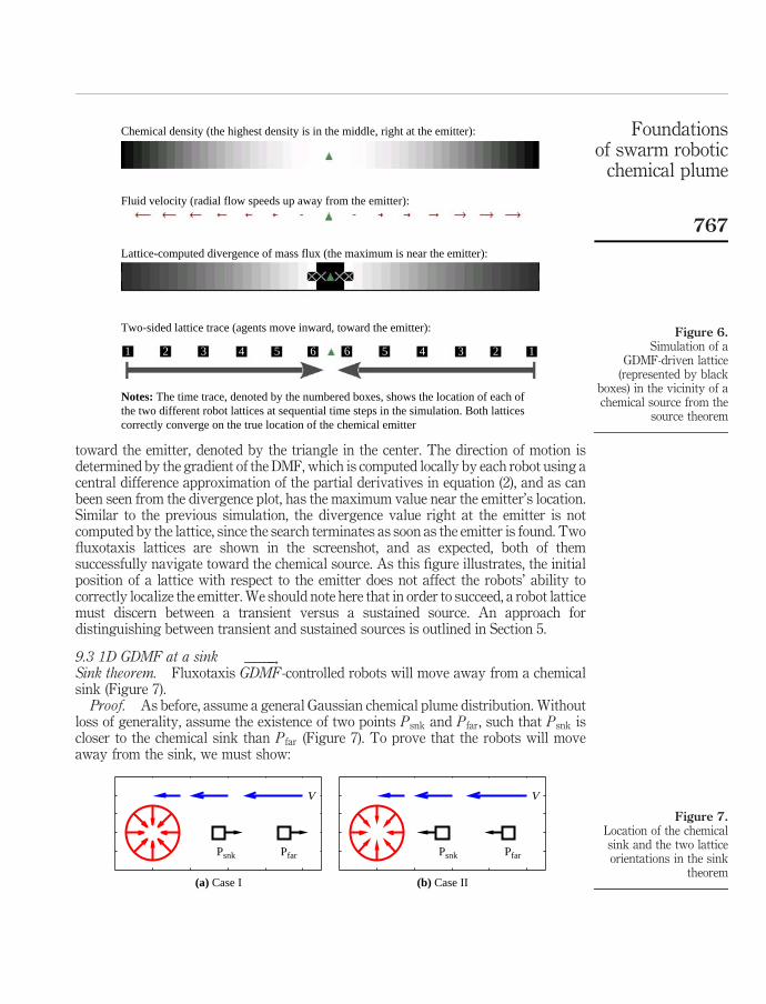
9.3 1D GDMF at a sinkSink theorem. Fluxotaxis

������!

GDMF-controlled robots will move away from a chemicalsink (Figure 7).

Proof. As before, assume a general Gaussian chemical plume distribution. Withoutloss of generality, assume the existence of two points Psnk and P far, such that Psnk iscloser to the chemical sink than P far (Figure 7). To prove that the robots will moveaway from the sink, we must show:

Figure 6.Simulation of a

GDMF-driven lattice(represented by black

boxes) in the vicinity of achemical source from the

source theorem

Chemical density (the highest density is in the middle, right at the emitter):

Fluid velocity (radial flow speeds up away from the emitter):

Notes: The time trace, denoted by the numbered boxes, shows the location of each ofthe two different robot lattices at sequential time steps in the simulation. Both latticescorrectly converge on the true location of the chemical emitter

Lattice-computed divergence of mass flux (the maximum is near the emitter):

Two-sided lattice trace (agents move inward, toward the emitter):

1 2 3 4 5 6 6 5 4 3 2 1

Figure 7.Location of the chemicalsink and the two latticeorientations in the sink

theorem

Psnk Pfar

V

(a) Case I

Psnk Pfar

V

(b) Case II

Foundationsof swarm robotic

chemical plume

767

u›r

›xþ r

›u

›x

� �snk

, u›r

›xþ r

›u

›x

� �far

: ð7Þ

Two cases result, based on the orientation of the lattice coordinate axis.Case I. Occurs when the lattice coordinate axis points in the opposite direction to thefluid flow, so that both usnk and ufar are negative (Figure 7). For this case, theassumptions are:

(1) ›2u=›x 2 $ 0;

(2) ›u=›x , 0; thus 0 $ usnk . ufar;

(3) ›2r=›x 2 # 0; and

(4) ›r=›x , 0 and therefore rsnk . rfar.

The robot will continue moving away from the sink if equation (7) is true. FromAssumption 1, we observe that:

›u

›x

� �snk

#›u

›x

� �far

:

Likewise, Assumption 3 implies:

›r

›x

� �snk

$›r

›x

� �far

:

The remaining assumptions with algebraic simplification prove that equation (7) istrue. A

Case II. if the direction of fluid flow and the lattice coordinate axis are the same,then:

(1) ›2u=›x 2 # 0;

(2) ›u=›x , 0; thus 0 # usnk , ufar;

(3) ›2r=›x 2 # 0; and

(4) ›r=›x . 0 and therefore rsnk . rfar.

From Assumptions 1 and 3, we conclude that:

›u

›x

� �snk

#›u

›x

� �far

and›r

›x

� �snk

#›r

›x

� �far

:

Algebraic simplification using Assumptions 2 and 4 proves Case II. ASimulation results for this theorem are shown in Figure 8. Confirming the

theoretical results, the high-density chemical build-up in the center of the environmentdoes not fool the fluxotaxis algorithm, which correctly avoids the local spike in thedensity by directing the robots (again represented by black boxes) to the outer edge ofthe tracing region, where as can be seen from the divergence plot, the maximum mass

flux divergence occurs. The sink theorem proves that a������!

GDMF-driven robot lattice willescape from a sink. However, a simple chemotaxis strategy is easily fooled by sinks,since by definition of a sink, ›r=›x . 0 going into the sink. The fluxotaxis scheme ismore robust in this case because it looks at the second-order partial derivative of r, and

IJICC2,4

768

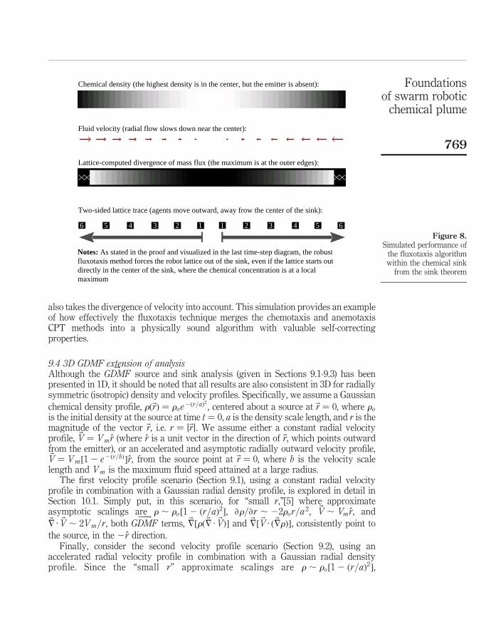
also takes the divergence of velocity into account. This simulation provides an exampleof how effectively the fluxotaxis technique merges the chemotaxis and anemotaxisCPT methods into a physically sound algorithm with valuable self-correctingproperties.

9.4 3D GDMF extension of analysisAlthough the

!

GDMF source and sink analysis (given in Sections 9.1-9.3) has beenpresented in 1D, it should be noted that all results are also consistent in 3D for radiallysymmetric (isotropic) density and velocity profiles. Specifically, we assume a Gaussian

chemical density profile, rð~rÞ ¼ roe2ðr=aÞ2 , centered about a source at ~r ¼ 0, where ro

is the initial density at the source at time t ¼ 0, a is the density scale length, and r is themagnitude of the vector ~r, i.e. r ¼ j~rj. We assume either a constant radial velocityprofile, ~V ¼ Vmr (where r is a unit vector in the direction of ~r, which points outwardfrom the emitter), or an accelerated and asymptotic radially outward velocity profile,~V ¼ Vm½1 2 e2ðr=bÞ�r, from the source point at ~r ¼ 0, where b is the velocity scalelength and Vm is the maximum fluid speed attained at a large radius.

The first velocity profile scenario (Section 9.1), using a constant radial velocityprofile in combination with a Gaussian radial density profile, is explored in detail inSection 10.1. Simply put, in this scenario, for “small r,”[5] where approximateasymptotic scalings are r , ro½1 2 ðr=aÞ2�, ›r=›r , 22ror=a

2, ~V , Vmr, and~7 · ~V , 2Vm=r, both

���!

GDMF terms, ~7½rð~7 · ~VÞ� and ~7½ ~V · ð~7rÞ�, consistently point to

the source, in the 2r direction.Finally, consider the second velocity profile scenario (Section 9.2), using an

accelerated radial velocity profile in combination with a Gaussian radial densityprofile. Since the “small r” approximate scalings are r , ro½1 2 ðr=aÞ2�,

Figure 8.Simulated performance of

the fluxotaxis algorithmwithin the chemical sink

from the sink theorem

Chemical density (the highest density is in the center, but the emitter is absent):

Fluid velocity (radial flow slows down near the center):

Lattice-computed divergence of mass flux (the maximum is at the outer edges):

Two-sided lattice trace (agents move outward, away frow the center of the sink):

6 5 4 3 2 1 1 2 3 4 5 6

Notes: As stated in the proof and visualized in the last time-step diagram, the robustfluxotaxis method forces the robot lattice out of the sink, even if the lattice starts outdirectly in the center of the sink, where the chemical concentration is at a localmaximum

Foundationsof swarm robotic

chemical plume

769

›r=›r , 22ror=a2, ~V , Vmðr=bÞr, and ~7 · ~V , ð3Vm=bÞð1 2 2r=3bÞ, both

���!

GDMFterms once again consistently point to the source, in the 2r direction.

10. A theoretical analysis of fluxotaxis and chemotaxis in 3DThe previous section focused primarily on the merits of fluxotaxis in the context ofsources and sinks. In this section, we address the question of how well fluxotaxisperforms in a 3D environment in the absence of sinks and sources other than the onesource – the emitter. We assume here that diffusion dominates and advection plays aperipheral and subsidiary role. Since chemotaxis is the most popular CPT methoddesigned to address diffusion, we analyze both fluxotaxis and chemotaxis with a focuson chemical diffusion.

To emphasize diffusion, here and in all of the appendices the flow speed is assumedto be temporally invariant, where the velocity field has a constant radial component.The derivation in this section decomposes the density r into its 3D components, anddelves deeper into the analysis that compares fluxotaxis with chemotaxis assumingtwo specific, but common types of emitters. Since we focus more on the chemical andless on the advective flow, we further refine our notion of the chemical density, r. Inparticular, it is useful to consider a particle number density formulation, nð~r; tÞ,

sometimes written as simply n, at a 3D spatial coordinate ~r ¼ xiþ yjþ zk, and time t.The particle number density n is the chemical particle count per unit volume. Then, themass density can be split up into its components, i.e. r ¼ mn, which is the mass m ofeach chemical particle times the number density n. Therefore, our prior expression for

the mass flux, r ~V, can be rewritten as mn ~V. Likewise, the 3D density diffusionequation can be written in terms of n as:

›nð~r; tÞ

›t¼ D72nð~r; tÞ: ð8Þ

This equation describes the evolution of the density of particles, nð~r; tÞ, as a function ofthe spatial coordinate, ~r, and time, t. It is particularly useful to consider a temporalinitial condition (t ¼ 0) where all the N particles are contained at the origin (~r ¼ ~0),represented as a Dirac delta function particle source, wherenð~r; 0Þ ¼ Nd 3ð~rÞ ¼ NdðxÞdð yÞdðzÞ. In Section 6.2, we showed that the diffusioncoefficient D is proportional to the square of the mean free path, lmfp, divided by thecollision time, tcoll, or D/ l2

mfp=tcoll:The conserved total number of particles (by the conservation of mass principle) is:

N ¼

Z 1

21

nð~r; tÞd3~r ¼

Z 1

21

nð~r; 0Þd3~r ¼

Z 1

21

Nd 3ð~rÞd3~r:

Using a Green’s function technique, we can solve the diffusion equation (8) for any typeof emitter (Appendix 1.1). A Green’s function is a Delta function source solution ofinhomogeneous partial differential equations with boundary conditions. Ultimately,the Green’s function for the diffusion equation can be used by integrating over theemitter source of particles to achieve the density solution for any localized particleemitter source. Appendix 1.2 provides a detailed solution for a single-puff emitter, and1.3 addresses the case for a continuously emitting constant-speed emitter. Thefollowing two subsections address each of these cases, in turn.

IJICC2,4

770

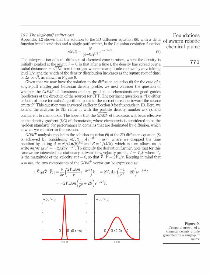
10.1 The single-puff emitter caseAppendix 1.2 shows that the solution to the 3D diffusion equation (8), with a deltafunction initial condition and a single-puff emitter, is the Gaussian evolution function:

nð~r; tÞ ¼N

ð4pDtÞ3=2e2r 2=4Dt: ð9Þ

The interpretation of such diffusion of chemical concentration, where the density isinitially peaked at the origin, ~r ¼ ~0, is that after a time t, the density has spread over aradial distance r <

ffiffiffiffiffiffiffiffi4Dt

pfrom the origin, where the amplitude is down by an e-folding

level 1=e, and the width of the density distribution increases as the square root of time,or Dr /

ffiffit

p, as shown in Figure 9.

Given that we now have the solution to the diffusion equation (8) for the case of asingle-puff emitter and Gaussian density profile, we next consider the question of

whether the������!

GDMF of fluxotaxis and the gradient of chemotaxis are good guides(predictors of the direction of the source) for CPT. The pertinent question is, “Do eitheror both of these formulas/algorithms point in the correct direction toward the sourceemitter?” This question was answered earlier in Section 9 for fluxotaxis in 1D. Here, weextend the analysis to 3D, refine it with the particle density number nð~r; tÞ, and

compare it to chemotaxis. The hope is that the������!

GDMF of fluxotaxis will be as effective

as the density gradient (!

DG) of chemotaxis, where chemotaxis is considered to be the“golden standard” for performance in domains that are dominated by diffusion, whichis what we consider in this section.

������!

GDMF analysis applied to the solution equation (9) of the 3D diffusion equation (8)is achieved by considering nð~r; tÞ ¼ Ae2Br 2

¼ nð~rÞ, where we dropped the timenotation by letting A ¼ N=ð4pDtÞ3=2 and B ¼ 1=ð4DtÞ, which in turn allows us towrite ›n=›r as n0 ¼ 22ABre2Br 2

. To simplify the derivation further, note that for thiscase we are interested in a stationary outward flow velocity profile, ~V ¼ Vor, where Vo

is the magnitude of the velocity at t ¼ 0, so that ~7 · ~V ¼ 2Vo=r. Keeping in mind that

r ¼ mn, the two components of the������!

GDMF vector can be expressed as:

1: ~7½rð~7 · ~VÞ� ¼›

›r

2VoAm

re2Br 2

� �r ¼ 2VoAm

21

r 22 2B

� �e2Br 2

r

¼ 22VoAm1

r 2þ 2B

� �e2Br 2

r:

Figure 9.Temporal growth of a

chemical density profilegenerated by a single-puff

source

n (r, t=0)

r = 0

→ ← (∆ r ~ 0) → ← ∆ r ∝ √ t

n (r, t>0)

r = 0

Foundationsof swarm robotic

chemical plume

771

2: ~7½ ~V · ð~7rÞ� ¼ 22ABm›

›rVore

2Br 2� �

r ¼ 22VoABm 1 2 2Br 2�

e2Br 2

r:

Substituting these values into the������!

GDMF (equation (4)) yields:

������!

GDMF ¼ m~7 ~7 · ðn ~VÞh i

¼ 22mVoAB 3 þ1

Br 22 2Br 2

� �e2Br 2

r:

For plume-tracing robots inside the inflection point ro ¼ 1=ffiffiffiffiffiffi2B

p(i.e. the region where

CPT is predictive), where:

n00ðroÞ ¼ 22AB 1 2 2Br2o

� e2Br2

o ¼ 0;

so that n00 , 0 for 0 # r , ro, the������!

GDMF vector correctly predicts the source directionto be:

sGDMF ¼

������!

GDMF

j������!

GDMFj¼ 2r:

Further assurance is provided by the fact that in the limit:

r!0lim j

������!

GDMFj!1; ð10Þ

r!rolim j

������!

GDMFj! 8mVoAB . 0; ð11Þ

indicating that the������!

GDMF vector is an effective and accurate source direction predictorfor all of the relevant radial domains.

Next, consider a chemotaxis-driven robot, which tracks the density gradient!

DG ¼ ~7n. For the same Gaussian density diffusion function:!

DG ¼ ~7 Ae2Br 2h i

¼›

›rAe2Br 2

h ir ¼ 22ABre2Br 2

r:

While this simpler scheme also predicts the correct source direction:

sDG ¼

!

DG

j!

DGj¼ 2r;

the problem with chemotaxis-guided search is that for the radial flow configuration,where the chemical density profile contains a maximum point at ~r ¼ ~0 (Figure 9), themagnitude DG of

!

DG goes to zero when ~r! ~0, i.e.:

~r!~0lim j

!

DGj ¼r!0lim 2ABre2Br 2

¼ 0:

This means that as chemotaxis-operated vehicles approach the source, their navigation

vector!

DG disappears. In contrast to this, the quality of the������!

GDMF prediction is

maximized at the source location, as shown in (10), so that the magnitude of������!

GDMF is

highest near the origin of the plume, since j������!

GDMFj!MAX as ~r! ~0, and the

predictive capability of������!

GDMF increases as fluxotaxis-controlled vehicles approach the

IJICC2,4

772

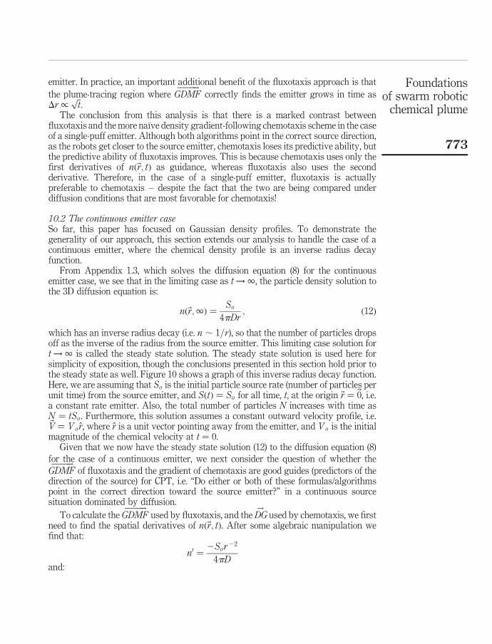
emitter. In practice, an important additional benefit of the fluxotaxis approach is that

the plume-tracing region where������!

GDMF correctly finds the emitter grows in time asDr /

ffiffit

p.

The conclusion from this analysis is that there is a marked contrast betweenfluxotaxis and the more naıve density gradient-following chemotaxis scheme in the caseof a single-puff emitter. Although both algorithms point in the correct source direction,as the robots get closer to the source emitter, chemotaxis loses its predictive ability, butthe predictive ability of fluxotaxis improves. This is because chemotaxis uses only thefirst derivatives of nð~r; tÞ as guidance, whereas fluxotaxis also uses the secondderivative. Therefore, in the case of a single-puff emitter, fluxotaxis is actuallypreferable to chemotaxis – despite the fact that the two are being compared underdiffusion conditions that are most favorable for chemotaxis!

10.2 The continuous emitter caseSo far, this paper has focused on Gaussian density profiles. To demonstrate thegenerality of our approach, this section extends our analysis to handle the case of acontinuous emitter, where the chemical density profile is an inverse radius decayfunction.

From Appendix 1.3, which solves the diffusion equation (8) for the continuousemitter case, we see that in the limiting case as t !1, the particle density solution tothe 3D diffusion equation is:

nð~r;1Þ ¼So

4pDr; ð12Þ

which has an inverse radius decay (i.e. n , 1=r), so that the number of particles dropsoff as the inverse of the radius from the source emitter. This limiting case solution fort !1 is called the steady state solution. The steady state solution is used here forsimplicity of exposition, though the conclusions presented in this section hold prior tothe steady state as well. Figure 10 shows a graph of this inverse radius decay function.Here, we are assuming that So is the initial particle source rate (number of particles perunit time) from the source emitter, and SðtÞ ¼ So for all time, t, at the origin ~r ¼ ~0, i.e.a constant rate emitter. Also, the total number of particles N increases with time asN ¼ tSo. Furthermore, this solution assumes a constant outward velocity profile, i.e.~V ¼ Vor, where r is a unit vector pointing away from the emitter, and Vo is the initialmagnitude of the chemical velocity at t ¼ 0.

Given that we now have the steady state solution (12) to the diffusion equation (8)

for the case of a continuous emitter, we next consider the question of whether the������!

GDMF of fluxotaxis and the gradient of chemotaxis are good guides (predictors of thedirection of the source) for CPT, i.e. “Do either or both of these formulas/algorithmspoint in the correct direction toward the source emitter?” in a continuous sourcesituation dominated by diffusion.

To calculate the������!

GDMF used by fluxotaxis, and the!

DG used by chemotaxis, we firstneed to find the spatial derivatives of nð~r; tÞ. After some algebraic manipulation wefind that:

n0 ¼2Sor

22

4pDand:

Foundationsof swarm robotic

chemical plume

773

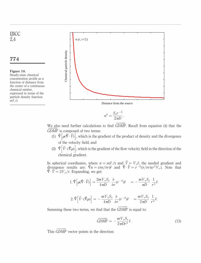
n00 ¼Sor

23

2pD:

We also need further calculations to find������!

GDMF . Recall from equation (4) that the������!

GDMF is composed of two terms:

(1) ~7 rð~7 · ~VÞh i

, which is the gradient of the product of density and the divergence

of the velocity field; and

(2) ~7 ~V · ð~7rÞh i

, which is the gradient of the flow velocity field in the direction of the

chemical gradient.

In spherical coordinates, where n ¼ nð~r; tÞ and ~V ¼ Vor, the needed gradient anddivergence results are: ~7n ¼ ð›n=›rÞr and ~7 · ~V ¼ r22ð›=›rÞðr 2VoÞ. Note that~7 · ~V ¼ 2Vo=r. Expanding, we get:

1: ~7 rð~7 · ~VÞh i

¼2mVoSo

4pD

›

›rðr22Þr ¼ 2

mVoSo

pD

1

r 3r:

2: ~7 ~V · ð~7rÞh i

¼ 2mVoSo

4pD

›

›rðr22Þr ¼

mVoSo

2pD

1

r 3r:

Summing these two terms, we find that the������!

GDMF is equal to:

������!

GDMF ¼ 2mVoSo

2pDr 3r: ð13Þ

This������!

GDMF vector points in the direction:

Figure 10.Steady-state chemicalconcentration profile as afunction of distance fromthe center of a continuouschemical emitter,expressed in terms of theparticle density functionnð~r; tÞ

n (r, t=∝)

Distance from the source

Che

mic

al p

artic

le d

ensi

ty

IJICC2,4

774

sGDMF ¼

������!

GDMF

j������!

GDMFj¼ 2r:

In other words, the������!

GDMF points toward the origin in a radially symmetric stationaryflow. This is exactly as desired.

Now, consider the density gradient,!

DG, approach used by chemotaxis:

!

DG ¼ n0r ¼ 2So

4pDr 2r: ð14Þ

We can see that chemotaxis also predicts the correct source direction since:

sDG ¼

!

DG

j!

DGj¼ 2r:

The conclusion is that both the������!

GDMF and the!

DG vectors point in the correct sourcedirection, and therefore fluxotaxis is as effective as chemotaxis for CPT domains wherediffusion dominates the spread of the chemical away from a continuous emitter. This isa very reassuring result.

In addition to pointing toward the source emitter, both������!

GDMF and!

DG have anotheradvantage in the case of a continuous chemical source: they maximize their values at the

emitter[6], ~r ¼ ~0, so that j������!

GDMFj!MAX . Thus, the predictive capabilities of������!

GDMF

and!

DG are both maximized close to the source emitter. However, it should be noted from

equations (13) and (14) that as ~r! ~0, the magnitude of the fluxotaxis predictor,

j������!

GDMFj / r23, becomes larger than that of the chemotaxis predictor, j!

DGj / r22.

11. Experimental confirmation of the theoryOur theory predicts that fluxotaxis should be an exceptionally adept CPT strategy,because it is based on fluid dynamics principles of source emitters. Now that we havefully developed our theory, let us consider how these results transfer to realistic 2Dsimulated chemical plume scenarios. In particular, how do the three CPT strategies(chemotaxis, anemotaxis and fluxotaxis) perform on plumes within varying flowregimes, such as laminar and turbulent? How do they perform under realisticconditions such as obstacles of varying number and size, anisotropic emitters, andunpredictable local variations in chemical density?

To address these questions, we have explored the performance of the three CPTstrategies in the context of a “standard” CPT simulator that allows methodicalperturbations of the emitter, flow, and simulated robot swarm characteristics. This“standard” CPT simulator was developed by Farrell et al. (2002). It is specificallydesigned for running large numbers of computationally efficient CPT experiments. Theinstantaneous and time-averaged results, as well as the multi-scale properties, of thissimulator match those of real-world chemical plumes. Essentially, chemical puffs areemitted from a stationary chemical source emitter, and are carried advectively by theambient wind flow. The regularity and frequency of puff emissions imply that thissimulation more accurately models how a continuous, rather than a single-puff, emitterwould act in the real world. Both advection and diffusion are modeled. The airborneemission is typically anisotropic, and it “meanders” dynamically as the wind currents

Foundationsof swarm robotic

chemical plume

775

change over time. We have extended Farrell et al.’s original simulator to model obstacles,using fluid boundary conditions.

Many experiments have been run and there is only room here for a brief qualitativesummary of them. For all of the quantitative and other specifics (Zarzhitsky et al.,2004a, 2005; Zarzhitsky, 2008). We have varied the fluid flow to range from laminar toturbulent, varied the number and sizes of obstacles, the number and initial locations(e.g. initial distance from the emitter) of the simulated robots, and the inter-robotdistances, and we have defined a variety of practical performance metrics. The latterinclude the frequency of emitter enclosure and the time of first detection of the emitter.Realistic robot constraints are modeled, such as realistic dimensions, maximumacceleration, sensor recovery time, and sensor and communication ranges. Also, bothsynchronous and asynchronous (multi-threaded) versions of the simulation have beenimplemented and tested, with no noticeable differences in the results.

Our simulation results demonstrate that the performance of fluxotaxis isoutstanding, and it consistently outperforms chemotaxis and anemotaxis, based onall of our performance metrics (Zarzhitsky et al., 2004a, 2005; Zarzhitsky, 2008),regardless of the perturbations in the flow regime, number and sizes of obstacles, andall of the other independent parameter variations. Chemotaxis is frequently fooled bylocal density maxima, especially when the environment has obstacles, thereby giving itpoor “first arrival time” results. Anemotaxis often overshoots the emitter, therebygiving it poor “detection frequency” results. Fluxotaxis outperforms both chemotaxisand anemotaxis on both of these metrics[7].

In some of the experiments, the swarm size is increased methodically. The resultsdemonstrate that CPT is inherently a swarm application. The bigger the swarm, themore effective and efficient the robots are at CPT.

Many of these results have been further confirmed in two other simulations, namely,a simulation of an extremely challenging urban environment containing largeclosely-spaced buildings of different sizes and shapes that substantially occlude thechemical flow (Agassounon et al., 2009), and in a simulation of a deep oceanenvironment. For the latter, the CPT-driven robots are required to locate ahydrothermal vent, and there are sinks in the environment to fool the CPT on its waytoward the source vent (Spears, 2009). Chemotaxis (which tracks heat, salinityor turbidity gradients) consistently gets trapped by the sinks; anemotaxis does not gettrapped but it overshoots the hydrothermal vent. On the other hand, fluxotaxis fleesthe sinks and homes right in on the vent source, quickly, accurately, and consistently.This is excellent confirmation of our theoretical results in this paper.

Finally, recall that our theory in the previous Section 10.2 predicts that as the robotsget closer to a continuous emitter, the magnitude of the fluxotaxis predictor will becomelarger than that of the chemotaxis predictor. When the speed of the robots is directlyproportional to the magnitude of the virtual attractive force on them (toward the emitter),confirmation of this theoretical prediction should come in the form of faster convergenceof the robot swarm upon a nearby emitter when using fluxotaxis than when usingchemotaxis. We have in fact seen experimental confirmation. In particular, when

watching the simulation it can be seen that when a������!

GDMF-driven fluxotaxis group ofrobots is near a source, it very rapidly “snaps” right onto the emitter location, whereas achemotaxis-driven group of robots slowly moves toward the nearby emitter.

IJICC2,4

776

12. Summary and future workIn this paper, we presented an analysis of the CPT problem in the context of theprinciples of fluid dynamics. Our fluid-based physicomimetic approach is posed as aviable and important alternative to the biomimetic approaches outlined in Cowen (2002).The main focus of our research is a physics-based chemical source localization algorithmthat can be implemented on a swarm of autonomous cooperating mobile robots. Ourinterest in the physicomimetic engineering of intelligent multi-robot systems stems fromthe relative ease with which such designs and algorithms can be analyzed and perfected.This approach allows us to apply similar mathematical techniques for both the designand analysis of our robot systems. In particular, the field of fluid dynamics providesnumerous theoretical and experimental techniques that yield a great deal of insight intothe behavior of chemical flows. It is therefore intuitive to apply a physicomimeticsolution to a problem that has such a strong physical foundation.

The most immediate and practical contribution of this work is the development of arobust, theory-based chemical source identification procedure. We have shown how thedivergence of chemical mass flux can be used to identify any chemical emitter.Our source declaration method can be readily combined with any of the popular CPTalgorithms, such as chemotaxis or anemotaxis, to significantly improve the emitterlocalization accuracy with minimal changes to the existing design. The precision of oursource identification method increases with the number of simultaneous observationsof the chemical plume, which implies that the CPT performance can be improvedsubstantially by increasing the number of plume-tracing robots in the swarm, therebyrealizing the benefit of cooperation between multiple vehicles. The decentralized natureof our solution translates into unrestricted scalability and excellent resiliency of thephysics-based algorithm.

In addition to the development of the source identification procedure, weconstructed a complete plume-tracing algorithm called fluxotaxis to take advantage ofthe information contained within the chemical mass flux. We showed that fluxotaxis,having been developed from the fundamental principles of fluid dynamics, captures thesalient features of both chemotaxis and anemotaxis – the two CPT algorithms thathave been derived via emulation of biological systems. By relying on standardtheoretical fluid-dynamics analysis techniques, we show in this paper that a CPTsystem that follows the gradient of the DMF performs at least as well as thechemotaxis technique in the presence of a continuous chemical source, and it actuallyoutperforms chemotaxis on plumes produced by single-puff emitters. Complementaryexperimental results showing the superior performance of fluxotaxis over chemotaxisand anemotaxis on a wide variety of realistic laminar and turbulent chemical flowregimes, with obstacles present, are summarized here.

The experimental confirmation of our theoretical results (Section 11) demonstratesthat the application of the physicomimetic approach for swarm design facilitates thedevelopment of CPT algorithms whose behavior is predictable. The ability to setbounds on the anticipated task performance in a theory-guided manner opens the doorto the possibility of formalizing physicomimetic systems, thus widening the range ofpotential applications to include mission-critical tasks.

In conclusion, the theoretical framework we have established in this paper has beeninstrumental in allowing us to develop our algorithms further into a functioning CPTsystem, which we have implemented and tested under a variety of real-world

Foundationsof swarm robotic

chemical plume

777

conditions. In the future, we intend to test and compare CPT algorithms in a variety ofsophisticated simulators (Iacono and Reynolds, 2008), including 3D simulators. Wealso plan to compare the algorithms on observed real chemical plume data, such as thedata that we have collected from our University of Wyoming Distributed RoboticsLaboratory CPT chemical/wind tunnel, and the plume data collected by others(Crimaldi and Koseff, 2006).

Furthermore, we plan to compare CPT algorithms on our team of laboratory robots.Currently, the robots have chemical sensors, and the design and integration ofminiature anemometer sensors are in progress. Once these sensors have beenintegrated, the next step will be to test and compare all of the CPT algorithms,including fluxotaxis, on the robots under varying indoor and outdoor conditions. Ourultimate objective is to understand the pros and cons of each of these strategies, and toclearly identify their regions of expertise in the space of possible environments.

Notes

1. Multiple emitters induce a separation of the swarm into smaller sub-swarms (Zarzhitsky andSpears, 2005).

2. For an excellent and comprehensive survey of CPT approaches that is much more generalthan the one herein, and which includes a categorization of fluxotaxis as a swarm-basedstrategy (Kowadlo and Russell, 2008).

3. The 1D results in this section originally appeared in Zarzhitsky et al. (2004c).

4. Without an explicit global reference frame, robots can share their local coordinate systemsand establish a common frame of reference using standard transformations (Craig, 1989).

5. We use the expansion “small r” to mean that the lowest (nonzero) order Taylor seriesexpansions have been performed on all density and velocity terms.

6. If the velocity is discontinuous at ~r ¼ ~0, we can alternatively get the same result with lim~r!~0

.

7. Note that in general, any of the three CPT algorithms can get stuck at a local maximum thathas features of a fluid “source” but is not the true overall global source emitter. Without aglobal perspective of the fluid field, or an infinite-sized swarm, this is a potential problemwith any CPT strategy. A proper setting of the time period t can help fluxotaxis to overcomethis problem (Section 5).

References

Agassounon, W., Spears, W., Welsh, R., Zarzhitsky, D. and Spears, D. (2009), “Toxic plumesource localization in urban environments using collaborating robots”, paper presented atIEEE Conference on Technologies for Homeland Security.

Anderson, J.D. (1995), Computational Fluid Dynamics, McGraw-Hill, New York, NY.

Balkovsky, E. and Shraiman, B. (2002), “Olfactory search at high Reynolds number”, PNAS,Vol. 99 No. 20, pp. 12589-93.

Board on Atmospheric Sciences and Climate (2003), Tracking and Predicting the AtmosphericDispersion of Hazardous Material Releases: Implications for Homeland Security, NationalAcademies Press, Washington, DC.

Buscemi, L., Prati, M. and Sandini, G. (1994), “Cellular robotics: behaviour in pollutedenvironments”, paper presented at 2nd International Symposium on DistributedAutonomous Robotic Systems, Springer-Verlag, New York, NY.

IJICC2,4

778

Caldwell, S.L., D’Agostino, D.M., McGeary, R.A., Purdy, H.L., Schwartz, M.J., Weeter, G.K. andWyrsch, R.J. (1997), “Combating terrorism: federal agencies’ efforts to implement nationalpolicy and strategy”, Congressional Report GAO/NSIAD-97-254, Washington, DC,September 26.

Chemical Hazards and Poisons Division, HPA (2006), Chemical Hazards and Poisons Report,Chemical Hazards and Poisons Division, Health Protection Agency, London.

Coirier, W.J., Fricker, D.M., Furmanczyk, M. and Kim, S. (2005), “A computational fluid dynamicsapproach for urban area transport and dispersion modeling”, Env. Fluid Mech., Vol. 5 No. 5,pp. 443-79.

Cordesman, A.H. (2001), Defending America: Asymmetric and Terrorist Attacks with ChemicalWeapons, Center for Strategic and International Studies (CSIS), Washington, DC.

Cowen, E. (2002), Env. Fluid Mech., Vol. 2 Nos 1-2, special issue on Chemical Plume Tracing.

Craig, J.J. (1989), Introduction to Robotics: Mechanics and Control, Addison-Wesley, Reading, MA.

Crimaldi, J.P. and Koseff, J.R. (2006), “Structure of turbulent plumes from a momentumless sourcein a smooth bed”, Env. Fluid Mech., Vol. 6 No. 6, pp. 573-92.

Crimaldi, J.P., Koehl, M.A.R. and Koseff, J.R. (2002), “Effects of the resolution and kinematics ofolfactory appendages on the interception of chemical signals in a turbulent odor plume”,Env. Fluid Mech., Vol. 2, pp. 35-63 (special issue on Chemical Plume Tracing).

Cui, X., Hardin, C.T., Ragade, R.K. and Elmaghraby, A.S. (2004), “A swarm approach foremission sources localization”, Proceedings of the 16th IEEE International Conference onTools with Artificial Intelligence, IEEE Press, Piscataway, NJ, pp. 424-30.

Decuyper, J. and Keymeulen, D. (1991), “A reactive robot navigation system based on a fluiddynamics metaphor”, Lecture Notes in Computer Science – Parallel Problem Solving fromNature (PPSN I), Vol. 496, Springer, Berlin, pp. 356-62.

Farrell, J.A., Murlis, J., Li, W. and Carde, R.T. (2002), “Filament-based atmospheric dispersionmodel to achieve short time-scale structure of odor plumes”, Env. Fluid Mech., Vol. 2Nos 1/2, pp. 143-69 (special issue on Chemical Plume Tracing).

Feddema, J.T., Robinett, R.D. and Byrne, R.H. (2003), “An optimization approach to distributedcontrols of multiple robot vehicles”, Proceedings of the IEEE/RSJ International Conferenceon Intelligent Robots and Systems (IROS’03), IEEE Press, Piscataway, NJ.

Grasso, F. (2001), “Invertebrate-inspired sensory-motor systems and autonomous,olfactory-guided exploration”, Biol. Bull., Vol. 200, pp. 160-8.

Grasso, F. and Atema, J. (2002), “Integration of flow and chemical sensing for guidance ofautonomous marine robots in turbulent flows”, Env. Fluid Mech., Vol. 2 Nos 1/2, pp. 95-114,special issue on Chemical Plume Tracing.

Hayes, A., Martinoli, A. and Goodman, R. (2001), “Swarm robotic odor localization”, Proceedingsof the IEEE/RSJ International Conference on Intelligent Robots and Systems (IROS’01),Wailea.

Hsu, S.S. (2003), “Sensors may track terror’s fallout”, Washington Post, June 2, p. A01.

Hughes-Hallett, D., Gleason, A.M. and McCallum, W. (1998), Calculus, Single and Multivariable,Wiley, New York, NY.

Iacono, G.L. and Reynolds, A.M. (2008), “Modelling of concentrations along a moving observer inan inhomogeneous plume. Biological application: model of odour-mediated insect flights”,Env. Fluid Mech., Vol. 8 No. 2, pp. 147-68.

Ishida, H., Tanaka, H., Taniguchi, H. and Moriizumi, T. (2006), “Mobile robot navigation usingvision and olfaction to search for a gas/odor source”, Auton. Robots, Vol. 20 No. 3, pp. 231-8(special issue on Mobile Robot Olfaction).

Foundationsof swarm robotic

chemical plume

779

Ishida, H., Nakamoto, T., Moriizumi, T., Kikas, T. and Janata, J. (2001), “Plume-tracking robots:a new application of chemical sensors”, Biol. Bull., Vol. 200, pp. 222-6.

Jeremic, A. and Nehorai, A. (1998), “Design of chemical sensor arrays for monitoring disposalsites on the ocean floor”, IEEE J. Ocean Eng., Vol. 23 No. 4, pp. 334-43.

Justus, K., Murlis, J., Jones, C. and Carde, R. (2002), “Measurement of odor-plume structure ina wind tunnel using a photoionization detector and a tracer gas”, Env. Fluid Mech., Vol. 21Nos 1/2, pp. 115-42 (special issue on Chemical Plume Tracing).

Kazadi, S., Goodman, R., Tskikata, D., Green, D. and Lin, H. (2000), “An autonomous water vaporplume tracking robot using passive resistance polymer sensors”, Auton. Robots, Vol. 9No. 2, pp. 175-88.

Keymeulen, D. and Decuyper, J. (1994a), “The fluid dynamics applied to mobile robot motion:the stream field method”, Proceedings of the 1994 International Conference on Roboticsand Automation (ICRA’94), Vol. 4, IEEE Press, Piscataway, NJ, pp. 378-85.

Keymeulen, D. and Decuyper, J. (1994b), “The stream field method applied to mobile robotnavigation: a topological perspective”, in Cohn, A.G. (Ed.), Proceedings of the EleventhEuropean Conference on Artificial Intelligence (ECAI’94), Wiley, Chichester, pp. 699-703.

Kikas, T., Ishida, H., Webster, D. and Janata, J. (2001), “Chemical plume tracking. 1. Chemicalinformation encoding”, Anal. Chemistry, Vol. 73, pp. 3662-8.

Kowadlo, G. and Russell, R.A. (2008), “Robot odor localization: a taxonomy and survey”,Int. J. Robot. Res., Vol. 27 No. 8, pp. 869-94.

Krishnanand, K. and Ghose, D. (2006), “Glowworm swarm based optimization algorithm formultimodal functions with collective robotics applications”, Multiagent Grid Syst., Vol. 2No. 3, pp. 209-22 (special issue on Recent Progress in Distributed Intelligence).

Liao, Q. and Cowen, E. (2002), “The information content of a scalar plume – a plume tracingperspective”, Env. Fluid Mech., Vol. 2 Nos 1/2, pp. 9-34 (special issue on Chemical PlumeTracing).

Lilienthal, A. and Duckett, T. (2003), “Approaches to gas source tracing and declaration by purechemo-tropotaxis”, Proceedings of AMS, Karlsruhe, December 4-5, pp. 161-71.

Lilienthal, A., Zell, A., Wandel, M. and Weimar, U. (2001), “Experiences using gas sensors on anautonomous mobile robot”, Proceedings of the 4th European Workshop on AdvancedMobile Robots (EUROBOT’01), Lund, pp. 1-8.

Lilienthal, A., Ulmer, H., Frohlich, H., Stutzle, A., Werner, F. and Zell, A. (2004), “Gas sourcedeclaration with a mobile robot”, Proceedings of the IEEE International Conference onRobotics and Automation (ICRA’04), April 26-May 1, New Orleans, LA, pp. 1430-5.

Lytridis, C., Kadar, E. and Virk, G. (2006), “A systematic approach to the problem of odour sourcelocalization”, Auton. Robots, Vol. 20 No. 3, pp. 261-76, special issue on Mobile RobotOlfaction.

Marques, L., Nunes, U. and de Almeida, A. (2006), “Particle swarm-based olfactory guidedsearch”, Auton. Robots, Vol. 20 No. 3, pp. 277-87 (special issue on Mobile Robot Olfaction).

Parunak, H.V.D. and Brueckner, S. (2001), “Entropy and self-organization in multi-agentsystems”, Proceedings of the International Conference on Autonomous Agents(AGENTS’01), Montreal, pp. 124-30.

Russell, R.A., Kleeman, L. and Kennedy, S. (2000), “Using volatile chemicals to help locate targetsin complex environments”, Proceedings of the Australian Conference on Robotics andAutomation (ACRA’00), August 30-September 1, Melbourne.

IJICC2,4

780

Sandini, G., Lucarini, G. and Varoli, M. (1993), “Gradient driven self-organizing systems”,Proceedings of the IEEE/RSJ International Conference on Intelligent Robots and Systems(IROS’93), July 26-30, Yokohama.

Shinoda, T. (2003), “Koizumi’s top-down leadership in the anti-terrorism legislation: the impact ofpolitical institutional changes”, SAIS Review, Vol. 23 No. 1, pp. 19-34.

Song, Z. and Chen, Y. (2006), “Challenges and some results for the MAS-net project”, First JointEmergency Preparation and Response Meeting, pp. 258-64.

Spears, D. (2009), “Hydrothermal vent localization with a team of drones”, Universityof Wyoming Technical Report.

Spears, D., Zarzhitsky, D. and Thayer, D. (2005), in Parker, L., Schultz, A. and Schneider, F. (Eds),Multi-robot Systems: From Swarms to Intelligent Automata, Vol. III, Springer-Verlag,New York, NY, pp. 211-22.

Spears, W. and Gordon, D. (1999), “Using artificial physics to control agents”, Proceedings of theIEEE Conference on Information, Intelligence, and Systems (ICIIS’99), Rockville, MD,pp. 281-8.

Spears, W., Heil, R. and Zarzhitsky, D. (2005), “Artificial physics for mobile robot formations”,Proceedings of the IEEE International Conference on Systems, Man and Cybernetics(SMC’05), IEEE Press, Piscataway, NJ, pp. 2287-92.

Spears, W., Spears, D., Hamann, J. and Heil, R. (2004), “Distributed, physics-based control ofswarms of vehicles”, Auton. Robots, Vol. 17 Nos 2/3, pp. 137-62.

Spears, W., Hamann, J., Maxim, P., Kunkel, T., Zarzhitsky, D., Spears, D. and Karlsson, C. (2006),“Where are you?”, Proceedings of the SAB Swarm Robotics Workshop, Springer-Verlag,New York, NY, pp. 129-43.

Thayer, D. (2008), “Theoretical foundations of chemical plume tracing with continuous and puffsource emitters”, University of Wyoming Technical Report.

Vergassola, M., Villermaux, E. and Shraiman, B. (2007), “Infotaxis as a strategy for searchingwithout gradients”, Nature, Vol. 445 No. 7126, pp. 406-9.

Weissburg, M., Dusenbery, D., Ishida, H., Janata, J., Keller, T., Roberts, P. and Webster, D. (2002),“A multidisciplinary study of spatial and temporal scales containing information inturbulent chemical plume tracking”, Env. Fluid Mech., Vol. 2 Nos 1/2, pp. 65-94, specialissue on Chemical Plume Tracing.

Zarzhitsky, D. (2008), “A physics-based approach to chemical source localization using mobilerobotic swarms”, PhD thesis, University of Wyoming, Laramie, WY.

Zarzhitsky, D. and Spears, D. (2005), “Swarm approach to chemical source localization”,Proceedings of the IEEE International Conference on Systems, Man and Cybernetics(SMC’05), IEEE Press, Piscataway, NJ, pp. 1435-40.

Zarzhitsky, D., Spears, D. and Spears, W. (2004a), “Swarms for chemical plume tracing”,Proceedings of the IEEE Swarm Intelligence Symposium (SIS’04), IEEE Press, Piscataway,NJ, pp. 249-56.

Zarzhitsky, D., Spears, D. and Spears, W. (2005), “Distributed robots approach to chemical plumetracing”, Proceedings of the IEEE/RSJ International Conference on Intelligent Robots andSystems (IROS’05), IEEE Press, Piscataway, NJ, pp. 4034-9.

Zarzhitsky, D., Spears, D., Thayer, D. and Spears, W. (2004b), “A fluid dynamics approach tomulti-robot chemical plume tracing”, Proceedings of the Third International JointConference on Autonomous Agents and Multiagent Systems (AAMAS’04), IEEEComputer Society, Washington, DC, pp. 1476-7.

Foundationsof swarm robotic

chemical plume

781

Zarzhitsky, D., Spears, D., Thayer, D. and Spears, W. (2004c), “Agent-based chemical plumetracing using fluid dynamics”, Lecture Notes in Computer Science, Vol. 3328,Springer-Verlag, New York, NY, pp. 146-60.

Appendix 1. Supplementary derivations for the GDMF theory1.1. General solution to the 3D diffusion equationHere, we derive a general solution to the 3D diffusion equation for the density function, nð~r; tÞ:

›

›tnð~r; tÞ ¼ D72nð~r; tÞ;

where D is the diffusion coefficient that is defined in Section 6.2. We develop the needed Green’sfunction as the density solution for a Dirac delta function initial condition (t ¼ 0) of the chemicaldensity at the origin ~r ¼ ~0. The derivations assume time-independent velocity and acompressible fluid. SðtÞ denotes the number of particles emitted per unit time from the sourceemitter which, for convenience, is assumed to be located at the origin of the coordinate system.

The density solution, nð~r; tÞ, of the 3D diffusion equation is obtained by integrating theproduct of the Green’s function, Gðt; t0Þ, and the source Sðt0Þ, over time, t0. The Green’s function isdeveloped from the solution to the diffusion equation (assuming a delta function initial condition)using a time difference interval, t2 t0. The Green’s function is:

Gðt; t0Þ ¼1

½4pDðt2 t0Þ�3=2e2ðr 2=4Dðt2t0 ÞÞ;

and the time-evolved solution to the 3D diffusion equation is:

nð~r; tÞ ¼

Z t

0

Gðt; t0ÞSðt0Þdt0: ðA1Þ

This Green’s function propagates the source at every time t0. Here, it should be noted that thetotal number of particles emitted at the origin ~r ¼ ~0, over a time t, is N ¼

R t

0Sðt0Þdt0. This is

becauseR1

21Gðt; t0Þd3~r ¼ 1, or

R1

21½nð~r; tÞ�d3~r ¼

R t

0Sðt0Þdt0, which is defined as N. Note that d3~r

is an abbreviation for dxdydz. Recall from calculus thatR1

21d3~r ¼

R1

21

R1

21

R1

21dxdydz.

The formula for nð~r; tÞ in equation (A1) is the solution to the 3D density diffusion equation:

›

›tnð~r; tÞ ¼ D72nð~r; tÞ;

where 72nð~r; tÞ ¼ r22 ››rðr 2 ›n

›rÞ, for any source, SðtÞ, at ~r ¼ ~0. In addition, for a delta function

source, SðtÞ ¼ NdðtÞ, the usual density solution occurs, as in equation (9).Note that limt!t0Gðt; t

0Þ ¼ d 3ð~rÞ and ››tGðt; t0Þ ¼ D72Gðt; t0Þ. Consequently, for a density

source, SðtÞ, over the period of time t0 ¼ 0 to t, normalized to N, where N ¼R t

0Sðt0Þdt0, the 3D

density result for all space, ~r, is nð~r; tÞ ¼R t

0Gðt; t0ÞSðt0Þdt0. The proof is as follows:

Proof: Z 1

21

nð~r; tÞd3~r ¼

Z t

0

Z 1

21

Gðt; t0Þd3~r

� �Sðt0Þdt0 ¼

Z t

0

Sðt0Þdt0 ¼ N ;

whereR1

21Gðt; t0Þd3~r ¼ 1: For ~r – ~0, we can rewrite:

›

›tnð~r; tÞ ¼

Z t

0

›

›tGðt; t0Þ

� �Sðt0Þdt0D72nð~r; tÞ ¼

Z t

0

½D72Gðt; t0Þ�Sðt0Þdt0:

Finally, with:

IJICC2,4

782

›

›tGðt; t0Þ ¼ D72Gðt; t0Þ;

we can conclude that:

›

›tnð~r; tÞ ¼

Z t

0

D72Gðt; t0Þ �

Sðt0Þdt0 ¼ D72nð~r; tÞ: A

Thus, as previously stated, the density at all 3D spatial points ~r and time t $ 0, driven by a

source SðtÞ at ~r ¼ ~0, is correctly given by the integral:

nð~r; tÞ ¼

Z t

0

Gðt; t0ÞSðt0Þdt0:

This general solution to the 3D diffusion equation is instantiated for the specific cases ofsingle-puff and continuous emitters, in Appendices 1.2 and 1.3, respectively.

1.2. Solution to the 3D diffusion equation with a single-puff emitterIn this Appendix 1.2, we present the solution to the 3D diffusion equation that assumes asingle-puff emitter. In other words, the emitter ejects a single chemical puff and then shuts down.We assume a delta function initial condition, where SðtÞ ¼ NdðtÞ.

Thayer (2008) showed that the puff emitter solution to the 3D diffusion equation, with a deltafunction initial condition, is the Gaussian evolution function:

nð~r; tÞ ¼N

ð4pDtÞ3=2e2ðr 2=4DtÞ;

where N ¼R1

21nð~r; tÞd3~r, and nð~r; 0Þ ¼ Nd 3ð~rÞ. We can verify that this is the value of N as

follows[1]:Z 1

21

nð~r; tÞd3~r ¼

Z 1

21

Z 1

21

Z 1

21

N

ð4pDtÞ3=2e2ðx 2=4DtÞe2ð y 2=4DtÞe2ðz 2=4DtÞdxdydz

¼ N1ffiffiffiffiffiffiffiffiffiffiffi

4pDtp

Z 1

21

e2ðx 2=4DtÞdx

� �3

;

due to spatial symmetry. Finally, substituting x 2=4Dt ¼ u 2 so that dx ¼ffiffiffiffiffiffiffiffi4Dt

pdu, we obtain:

N1ffiffiffiffiffiffiffiffiffiffiffi

4pDtp

Z 1

21

e2ðx 2=4DtÞdx

� �3

¼ N1ffiffiffiffip

p

Z 1

21

e2u 2

du

� �3

¼ N ð1Þ3 ¼ N :

We can use this value of N to derive the initial condition solution nð~r; 0Þ. We now know that forall t, N ¼

R1

21nð~r; tÞd3~r. By taking the t! 0 limit of the density function, nð~r; tÞ, for the j~rj ¼ 0

and j~rj – 0 cases, where:

t!0lim nð~r; tÞ ¼

1; j~rj ¼ 0

0; j~rj – 0;

(;

and comparing this with the Dirac delta function definition, we can therefore conclude thatnð~r; 0Þ ¼ Nd 3ð~rÞ: Note that this solution to the diffusion equation with a single-puff emitter is theusual Gaussian profile with spatial width proportional to

ffiffiffiffiffiffiffiffi4Dt

p. See Figure 9 for a graph of this

profile. For the verification that this is the solution to the diffusion equation in the case of a puffemitter, see the complete mathematical proof in Thayer (2008).

Foundationsof swarm robotic

chemical plume

783

1.3. Solution of the 3D diffusion equation with a continuous emitterFor the case of a continuous chemical emitter, SðtÞ ¼ So, so that a fixed number of particles pertime step is being emitted at the ~r ¼ ~0 source location. For this case, the solution to equation (8) isgiven by:

nð~r; tÞ ¼ So

Z t

0

Gðt; t0Þdt0 ¼ So

Z t

0

1

½4pDðt2 t0Þ�3=2e2ðr 2=4Dðt2t0ÞÞdt0: ðA2Þ

Note that the total number of particles emitted from time 0 to time t is:

N ¼

Z 1

21

nð~r; tÞd3~r ¼ So

Z t

0

dt0Z 1

21

Gðt; t0Þd3~r ¼ So

Z t

0

ð1Þdt0 ¼ tSo:

In other words, N ¼ tSo.To make the diffusion equation solution simpler, as needed in Section 10.2, we solve the

integral in equation (A2). The solution to the Green’s function integral is found as follows.Starting with a change of variables ðt 2 t0Þ ¼ t and dt0 ¼ 2dt, we write:

nð~r; tÞ ¼ So

Z t

0

1

ð4pDtÞ3=2e2ðr 2=4DtÞdt:

Let u ¼ r=ðffiffiffiffiffiffiffiffi4Dt

pÞ, u 2 ¼ r 2=ð4DtÞ, t ¼ r 2=ð4Du 2Þ, and dt ¼ 2ð2r 2Þ=ð4Du 3Þdu, so that:

nð~r; tÞ ¼So

p 3=2

Z 1

r=ffiffiffiffiffi4Dt

p

r 2

2Du 3

u 3

r 3e2u 2

du ¼So

4pDr

2ffiffiffiffip

p

Z 1

r=ffiffiffiffiffi4Dt

p e2u 2

du:

Note that this expression is related to the probability integral, or the error function erf, which is

defined as erf ðaÞ ¼ 2=ffiffiffiffip

p R a

0 e2u 2

du. Here, a ¼ r=ffiffiffiffiffiffiffiffi4Dt

p, erf ð1Þ ¼ 1, and erf ð0Þ ¼ 0, while

ð2=ffiffiffiffip

pÞR a

0 e2u 2

duþ ð2=ffiffiffiffip

pÞR1

ae2u 2

du ¼ 1. Therefore, we have:

nð~r; tÞ ¼So

4pDr1 2 erf

rffiffiffiffiffiffiffiffi4Dt

p

� �� :

Consider two limiting cases of this solution:Case 1. For t ! 0, erf ð1Þ ¼ 1. This implies that nð~r; 0Þ ¼ 0 for j~rj . 0.Case 2. For t!1, erf ð0Þ ¼ 0. This implies that nð~r;1Þ ¼ So=ð4pDrÞ, which has an inverse

radius decay, as noted in Section 10.2 and shown in Figure 10. In fact, it is this Case 2 solutionthat is addressed in the main body of the paper.

Finally, note that for small distances r and large times t, where a ¼ r=ffiffiffiffiffiffiffiffi4Dt

pp 1, the Taylor

series expansion of the error function is useful:

erf ðaÞ ¼2ffiffiffiffip

p e2a 2X1n¼0

2n

1 · 3· · ·ð2nþ 1Þa 2nþ1;

with:

nð~r; tÞ ¼So

4pDr1 2 erf ðaÞf g:

In other words, we can solve for nð~r; tÞ computationally, using this expansion, at any point inspace and time – in order to calculate the GDMF. See Thayer (2008) for verification and acomplete mathematical proof that this is indeed the solution to the diffusion equation in the caseof a continuous emitter.

Note: 1. Recall from calculus thatR1

21d3~r ¼

R1

21

R1

21

R1

21dxdydz.

IJICC2,4

784

About the authors

Diana F. Spears received the PhD degree in Computer Science from the Universityof Maryland in 1990. She is currently an owner and senior research scientist atSwarmotics, LLC, and also an Adjunct Associate Professor in the ComputerScience Department at the University of Wyoming (UW). Previously, she workedat NASA Goddard Space Flight Center, the National Institute of Standards andTechnology, and as an Associate Professor of Computer Science at UW. She wasan Associate Editor for the Journal of Artificial Intelligence Research and is

currently on their Advisory Board. She is currently serving as an invited member on the AAAIPresidential Panel on the Future of Artificial Intelligence. She has over 80 publications, and isknown internationally for her expertise on swarm robotics and multi-robot chemical plumetracing. Her other research interests include behaviorally assured adaptive and machine learningsystems, and mathematical/graphical modeling and model reconstruction. Her personal web siteis: www.cs.uwyo.edu/,dspears. Diana F. Spears is the corresponding author and can becontacted at: dspears@swarmotics.com

David R. Thayer received the PhD degree in Plasma Physics from MIT in 1983.He has been a faculty member of the Department of Physics and Astronomy atthe UW since 2000. Previous positions have included: a senior scientist position atSAIC working directly under the CEO on projects including biotechnology, globalchange research, nanotechnology, submarine turbulent flows (DARPA funded),and fusion plasma transport (DOE funded), and a staff scientist position atLawrence Berkeley Laboratory working on ICRF heating through turbulent edge

plasma devices. Currently, in addition to CFD research with the Computer Science Department atUW, he works with the UW Mathematics and Electrical and Computer Engineering departmentson non-thermal plasma reactor analysis for hydrogen production. He teaches many of thegraduate and upper-division undergraduate physics courses at UW, including classicalmechanics, plasma physics, mathematical and computational physics and quantum mechanics.He is a member of the American Physical Society.

Dimitri V. Zarzhitsky received the PhD degree in Computer Science from the UWin 2008. He is an active participant in several ongoing research efforts betweengovernment agencies and university laboratories, overseeing design,development, and deployment of unmanned systems for both civilian andmilitary applications. Presently, he is working on improving effectiveness ofcooperative sensing and control algorithms for distributed autonomous systems.

Foundationsof swarm robotic

chemical plume

785

To purchase reprints of this article please e-mail: reprints@emeraldinsight.comOr visit our web site for further details: www.emeraldinsight.com/reprints