Embed Size (px)
Citation preview
1
Swarm Intelligence: Foundations, Perspectivesand Applications
Ajith Abraham1, He Guo2, and Hongbo Liu2
1 IITA Professorship Program, School of Computer Science and Engineering,Chung-Ang University, Seoul, 156-756, Korea. [email protected],http://www.softcomputing.net
2 Department of Computer Science, Dalian University of Technology, Dalian,116023, China. {guohe,lhb}@dlut.edu.cn
This chapter introduces some of the theoretical foundations of swarm intel-ligence. We focus on the design and implementation of the Particle SwarmOptimization (PSO) and Ant Colony Optimization (ACO) algorithms for var-ious types of function optimization problems, real world applications and datamining. Results are analyzed, discussed and their potentials are illustrated.
1.1 Introduction
Swarm Intelligence (SI) is an innovative distributed intelligent paradigm forsolving optimization problems that originally took its inspiration from thebiological examples by swarming, flocking and herding phenomena in verte-brates.
Particle Swarm Optimization (PSO) incorporates swarming behaviors ob-served in flocks of birds, schools of fish, or swarms of bees, and even hu-man social behavior, from which the idea is emerged [14, 7, 22]. PSO is apopulation-based optimization tool, which could be implemented and appliedeasily to solve various function optimization problems, or the problems thatcan be transformed to function optimization problems. As an algorithm, themain strength of PSO is its fast convergence, which compares favorably withmany global optimization algorithms like Genetic Algorithms (GA) [13], Sim-ulated Annealing (SA) [20, 27] and other global optimization algorithms. Forapplying PSO successfully, one of the key issues is finding how to map theproblem solution into the PSO particle, which directly affects its feasibilityand performance.
Ant Colony Optimization (ACO) deals with artificial systems that is in-spired from the foraging behavior of real ants, which are used to solve discrete
A. Abraham et al.: Swarm Intelligence: Foundations, Perspectives and Applications, Studies in
Computational Intelligence (SCI) 26, 3–25 (2006)
www.springerlink.com c© Springer-Verlag Berlin Heidelberg 2006
4 Ajith Abraham, He Guo, and Hongbo Liu
optimization problems [9]. The main idea is the indirect communication be-tween the ants by means of chemical pheromone trials, which enables themto find short paths between their nest and food.
This Chapter is organized as follows. Section 1.2 presents the canonicalPSO algorithm and its performance is compared with some global optimiza-tion algorithms. Further some extended versions of PSO is presented in Sec-tion 1.3 followed by some illustrations/applications in Section 1.4. Section1.5 presents the ACO algorithm followed by some illustrations/applicationsof ACO in Section 1.6 and Section 1.7. Some conclusions are also providedtowards the end, in Section 1.8.
1.2 Canonical Particle Swarm Optimization
1.2.1 Canonical Model
The canonical PSO model consists of a swarm of particles, which are initial-ized with a population of random candidate solutions. They move iterativelythrough the d-dimension problem space to search the new solutions, where thefitness, f , can be calculated as the certain qualities measure. Each particle hasa position represented by a position-vector xi (i is the index of the particle),and a velocity represented by a velocity-vector vi. Each particle remembersits own best position so far in a vector x#
i , and its j-th dimensional valueis x#
ij . The best position-vector among the swarm so far is then stored in avector x∗, and its j-th dimensional value is x∗
j . During the iteration time t,the update of the velocity from the previous velocity to the new velocity isdetermined by Eq.(1.1). The new position is then determined by the sum ofthe previous position and the new velocity by Eq.(1.2).
vij(t + 1) = wvij(t) + c1r1(x#ij(t) − xij(t)) + c2r2(x∗
j (t) − xij(t)). (1.1)
xij(t + 1) = xij(t) + vij(t + 1). (1.2)
where w is called as the inertia factor, r1 and r2 are the random numbers,which are used to maintain the diversity of the population, and are uniformlydistributed in the interval [0,1] for the j-th dimension of the i-th particle. c1
is a positive constant, called as coefficient of the self-recognition component,c2 is a positive constant, called as coefficient of the social component. FromEq.(1.1), a particle decides where to move next, considering its own experience,which is the memory of its best past position, and the experience of its mostsuccessful particle in the swarm. In the particle swarm model, the particlesearches the solutions in the problem space with a range [−s, s] (If the rangeis not symmetrical, it can be translated to the corresponding symmetricalrange.) In order to guide the particles effectively in the search space, themaximum moving distance during one iteration must be clamped in betweenthe maximum velocity [−vmax, vmax] given in Eq.(1.3):
1 Swarm Intelligence: Foundations, Perspectives and Applications 5
vij = sign(vij)min(|vij | , vmax). (1.3)
The value of vmax is p × s, with 0.1 ≤ p ≤ 1.0 and is usually chosen to bes, i.e. p = 1. The pseudo-code for particle swarm optimization algorithm isillustrated in Algorithm 1.
Algorithm 1 Particle Swarm Optimization Algorithm01. Initialize the size of the particle swarm n, and other parameters.02. Initialize the positions and the velocities for all the particles randomly.03. While (the end criterion is not met) do04. t = t + 1;05. Calculate the fitness value of each particle;06. x∗ = argminn
i=1(f(x∗(t − 1)), f(x1(t)), f(x2(t)), · · · , f(xi(t)), · · · , f(xn(t)));07. For i= 1 to n08. x#
i (t) = argminni=1(f(x#
i (t − 1)), f(xi(t));09. For j = 1 to Dimension10. Update the j-th dimension value of xi and vi
10. according to Eqs.(1.1), (1.2), (1.3);12. Next j13. Next i14. End While.
The end criteria are usually one of the following:
• Maximum number of iterations: the optimization process is terminatedafter a fixed number of iterations, for example, 1000 iterations.
• Number of iterations without improvement: the optimization process isterminated after some fixed number of iterations without any improve-ment.
• Minimum objective function error: the error between the obtained ob-jective function value and the best fitness value is less than a pre-fixedanticipated threshold.
1.2.2 The Parameters of PSO
The role of inertia weight w, in Eq.(1.1), is considered critical for the conver-gence behavior of PSO. The inertia weight is employed to control the impactof the previous history of velocities on the current one. Accordingly, the pa-rameter w regulates the trade-off between the global (wide-ranging) and local(nearby) exploration abilities of the swarm. A large inertia weight facilitatesglobal exploration (searching new areas), while a small one tends to facilitatelocal exploration, i.e. fine-tuning the current search area. A suitable valuefor the inertia weight w usually provides balance between global and localexploration abilities and consequently results in a reduction of the number

6 Ajith Abraham, He Guo, and Hongbo Liu
of iterations required to locate the optimum solution. Initially, the inertiaweight is set as a constant. However, some experiment results indicates thatit is better to initially set the inertia to a large value, in order to promoteglobal exploration of the search space, and gradually decrease it to get morerefined solutions [11]. Thus, an initial value around 1.2 and gradually reduc-ing towards 0 can be considered as a good choice for w. A better methodis to use some adaptive approaches (example: fuzzy controller), in which theparameters can be adaptively fine tuned according to the problems underconsideration [24, 16].
The parameters c1 and c2, in Eq.(1.1), are not critical for the convergenceof PSO. However, proper fine-tuning may result in faster convergence andalleviation of local minima. As default values, usually, c1 = c2 = 2 are used,but some experiment results indicate that c1 = c2 = 1.49 might provide evenbetter results. Recent work reports that it might be even better to choose alarger cognitive parameter, c1, than a social parameter, c2, but with c1 + c2 ≤4 [7].
The particle swarm algorithm can be described generally as a populationof vectors whose trajectories oscillate around a region which is defined byeach individual’s previous best success and the success of some other particle.Various methods have been used to identify some other particle to influencethe individual. Eberhart and Kennedy called the two basic methods as “gbestmodel” and “lbest model” [14]. In the lbest model, particles have informationonly of their own and their nearest array neighbors’ best (lbest), rather thanthat of the entire group. Namely, in Eq.(1.4), gbest is replaced by lbest in themodel. So a new neighborhood relation is defined for the swarm:
vid(t+1) = w∗vid(t)+c1∗r1∗(pid(t)−xid(t))+c2∗r2∗(pld(t)−xid(t)). (1.4)
xid(t + 1) = xid(t) + vid(t + 1). (1.5)
In the gbest model, the trajectory for each particle’s search is influenced bythe best point found by any member of the entire population. The best particleacts as an attractor, pulling all the particles towards it. Eventually all particleswill converge to this position. The lbest model allows each individual to beinfluenced by some smaller number of adjacent members of the populationarray. The particles selected to be in one subset of the swarm have no directrelationship to the other particles in the other neighborhood. Typically lbestneighborhoods comprise exactly two neighbors. When the number of neighborsincreases to all but itself in the lbest model, the case is equivalent to thegbest model. Some experiment results testified that gbest model convergesquickly on problem solutions but has a weakness for becoming trapped inlocal optima, while lbest model converges slowly on problem solutions but isable to “flow around” local optima, as the individuals explore different regions.The gbest model is recommended strongly for unimodal objective functions,while a variable neighborhood model is recommended for multimodal objectivefunctions.
1 Swarm Intelligence: Foundations, Perspectives and Applications 7
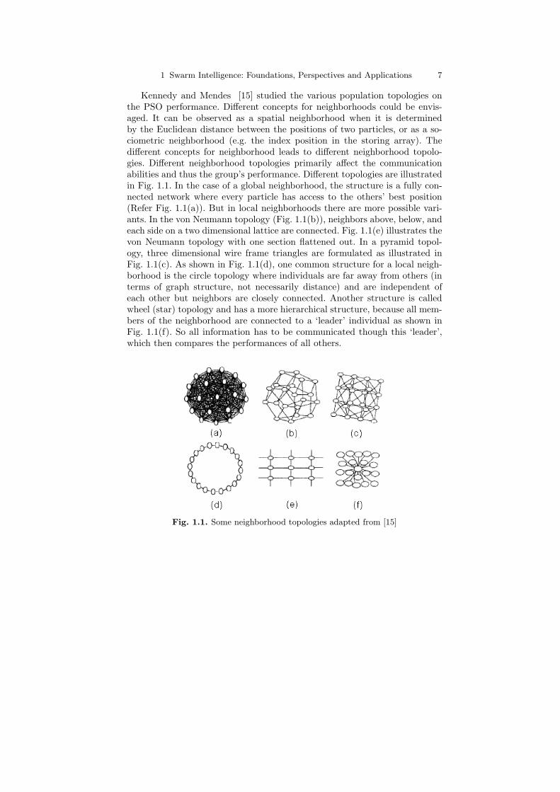
Kennedy and Mendes [15] studied the various population topologies onthe PSO performance. Different concepts for neighborhoods could be envis-aged. It can be observed as a spatial neighborhood when it is determinedby the Euclidean distance between the positions of two particles, or as a so-ciometric neighborhood (e.g. the index position in the storing array). Thedifferent concepts for neighborhood leads to different neighborhood topolo-gies. Different neighborhood topologies primarily affect the communicationabilities and thus the group’s performance. Different topologies are illustratedin Fig. 1.1. In the case of a global neighborhood, the structure is a fully con-nected network where every particle has access to the others’ best position(Refer Fig. 1.1(a)). But in local neighborhoods there are more possible vari-ants. In the von Neumann topology (Fig. 1.1(b)), neighbors above, below, andeach side on a two dimensional lattice are connected. Fig. 1.1(e) illustrates thevon Neumann topology with one section flattened out. In a pyramid topol-ogy, three dimensional wire frame triangles are formulated as illustrated inFig. 1.1(c). As shown in Fig. 1.1(d), one common structure for a local neigh-borhood is the circle topology where individuals are far away from others (interms of graph structure, not necessarily distance) and are independent ofeach other but neighbors are closely connected. Another structure is calledwheel (star) topology and has a more hierarchical structure, because all mem-bers of the neighborhood are connected to a ‘leader’ individual as shown inFig. 1.1(f). So all information has to be communicated though this ‘leader’,which then compares the performances of all others.
Fig. 1.1. Some neighborhood topologies adapted from [15]
8 Ajith Abraham, He Guo, and Hongbo Liu
1.2.3 Performance Comparison with Some Global OptimizationAlgorithms
We compare the performance of PSO with Genetic Algorithm (GA) [6, 13]and Simulated Annealing (SA)[20, 27]. GA and SA are powerful stochasticsearch and optimization methods, which are also inspired from biological andthermodynamic processes.
Genetic algorithms mimic an evolutionary natural selection process. Gen-erations of solutions are evaluated according to a fitness value and only thosecandidates with high fitness values are used to create further solutions viacrossover and mutation procedures.
Simulated annealing is based on the manner in which liquids freeze ormetals re-crystalize in the process of annealing. In an annealing process, amelt, initially at high temperature and disordered, is slowly cooled so thatthe system at any time is approximately in thermodynamic equilibrium. Interms of computational simulation, a global minimum would correspond tosuch a ”frozen” (steady) ground state at the temperature T=0.
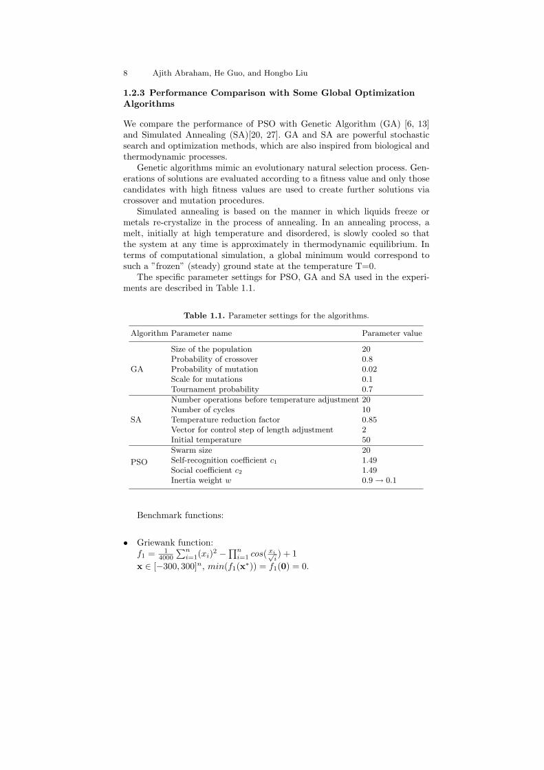
The specific parameter settings for PSO, GA and SA used in the experi-ments are described in Table 1.1.
Table 1.1. Parameter settings for the algorithms.
Algorithm Parameter name Parameter value
Size of the population 20Probability of crossover 0.8
GA Probability of mutation 0.02Scale for mutations 0.1Tournament probability 0.7
Number operations before temperature adjustment 20Number of cycles 10
SA Temperature reduction factor 0.85Vector for control step of length adjustment 2Initial temperature 50
Swarm size 20Self-recognition coefficient c1 1.49PSOSocial coefficient c2 1.49Inertia weight w 0.9 → 0.1
Benchmark functions:
• Griewank function:f1 = 1
4000
∑ni=1(xi)2 −
∏ni=1 cos( xi√
i) + 1
x ∈ [−300, 300]n, min(f1(x∗)) = f1(0) = 0.
1 Swarm Intelligence: Foundations, Perspectives and Applications 9
• Schwefel 2.26 function:f2 = 418.9829n −
∑ni=1(xisin(
√|xi|))
x ∈ [−500, 500]n, min(f2(x∗)) = f2(0) = 0.• Quadric function:
f3 =∑n
i=1(∑i
j=1 xj)2
x ∈ [−100, 100]n, min(f3(x∗)) = f3(0) = 0.
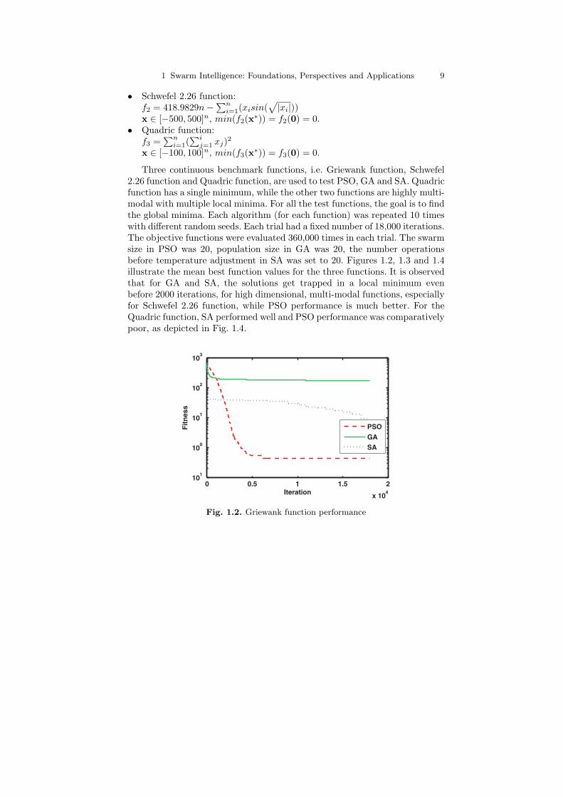
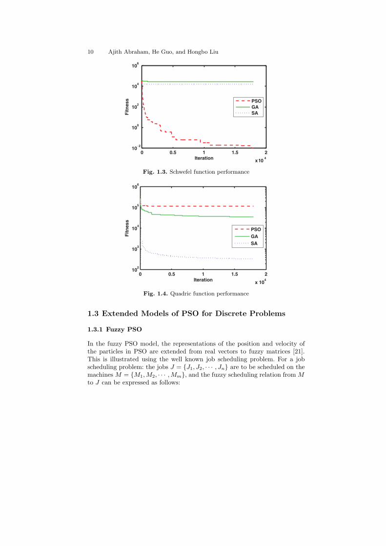
Three continuous benchmark functions, i.e. Griewank function, Schwefel2.26 function and Quadric function, are used to test PSO, GA and SA. Quadricfunction has a single minimum, while the other two functions are highly multi-modal with multiple local minima. For all the test functions, the goal is to findthe global minima. Each algorithm (for each function) was repeated 10 timeswith different random seeds. Each trial had a fixed number of 18,000 iterations.The objective functions were evaluated 360,000 times in each trial. The swarmsize in PSO was 20, population size in GA was 20, the number operationsbefore temperature adjustment in SA was set to 20. Figures 1.2, 1.3 and 1.4illustrate the mean best function values for the three functions. It is observedthat for GA and SA, the solutions get trapped in a local minimum evenbefore 2000 iterations, for high dimensional, multi-modal functions, especiallyfor Schwefel 2.26 function, while PSO performance is much better. For theQuadric function, SA performed well and PSO performance was comparativelypoor, as depicted in Fig. 1.4.
0 0.5 1 1.5 2
x 104
101
100
101
102
103
Iteration
Fit
nes
s
PSO
GASA
Fig. 1.2. Griewank function performance
10 Ajith Abraham, He Guo, and Hongbo Liu
0 0.5 1 1.5 2
x 104
10−2
100
102
104
106
Iteration
Fit
nes
s PSOGASA
Fig. 1.3. Schwefel function performance
0 0.5 1 1.5 2
x 104
102
103
104
105
106
Iteration
Fit
nes
s
PSOGASA
Fig. 1.4. Quadric function performance
1.3 Extended Models of PSO for Discrete Problems
1.3.1 Fuzzy PSO
In the fuzzy PSO model, the representations of the position and velocity ofthe particles in PSO are extended from real vectors to fuzzy matrices [21].This is illustrated using the well known job scheduling problem. For a jobscheduling problem: the jobs J = {J1, J2, · · · , Jn} are to be scheduled on themachines M = {M1,M2, · · · ,Mm}, and the fuzzy scheduling relation from Mto J can be expressed as follows:
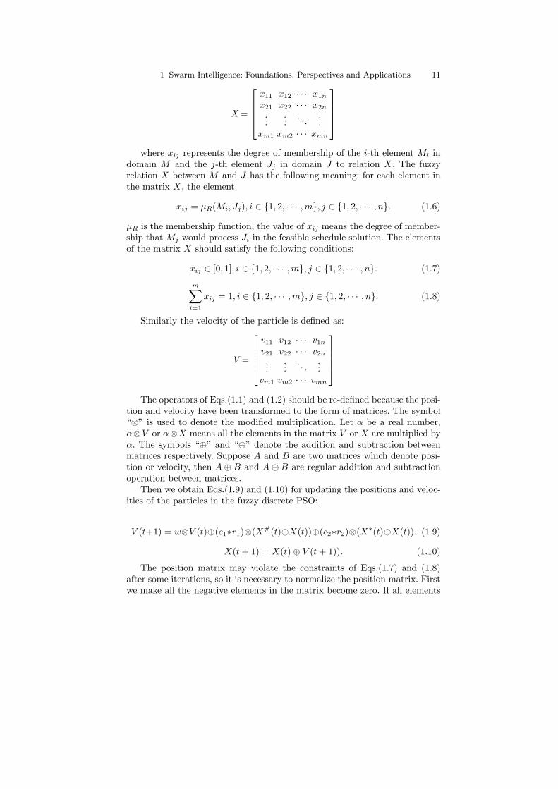
1 Swarm Intelligence: Foundations, Perspectives and Applications 11
X =
⎡
⎢⎢⎢⎣
x11 x12 · · · x1n
x21 x22 · · · x2n
......
. . ....
xm1 xm2 · · · xmn
⎤
⎥⎥⎥⎦
where xij represents the degree of membership of the i-th element Mi indomain M and the j-th element Jj in domain J to relation X. The fuzzyrelation X between M and J has the following meaning: for each element inthe matrix X, the element
xij = µR(Mi, Jj), i ∈ {1, 2, · · · ,m}, j ∈ {1, 2, · · · , n}. (1.6)
µR is the membership function, the value of xij means the degree of member-ship that Mj would process Ji in the feasible schedule solution. The elementsof the matrix X should satisfy the following conditions:
xij ∈ [0, 1], i ∈ {1, 2, · · · ,m}, j ∈ {1, 2, · · · , n}. (1.7)
m∑
i=1
xij = 1, i ∈ {1, 2, · · · ,m}, j ∈ {1, 2, · · · , n}. (1.8)
Similarly the velocity of the particle is defined as:
V =
⎡
⎢⎢⎢⎣
v11 v12 · · · v1n
v21 v22 · · · v2n
......
. . ....
vm1 vm2 · · · vmn
⎤
⎥⎥⎥⎦
The operators of Eqs.(1.1) and (1.2) should be re-defined because the posi-tion and velocity have been transformed to the form of matrices. The symbol“⊗” is used to denote the modified multiplication. Let α be a real number,α⊗V or α⊗X means all the elements in the matrix V or X are multiplied byα. The symbols “⊕” and “�” denote the addition and subtraction betweenmatrices respectively. Suppose A and B are two matrices which denote posi-tion or velocity, then A ⊕ B and A � B are regular addition and subtractionoperation between matrices.
Then we obtain Eqs.(1.9) and (1.10) for updating the positions and veloc-ities of the particles in the fuzzy discrete PSO:
V (t+1) = w⊗V (t)⊕(c1∗r1)⊗(X#(t)�X(t))⊕(c2∗r2)⊗(X∗(t)�X(t)). (1.9)
X(t + 1) = X(t) ⊕ V (t + 1)). (1.10)
The position matrix may violate the constraints of Eqs.(1.7) and (1.8)after some iterations, so it is necessary to normalize the position matrix. Firstwe make all the negative elements in the matrix become zero. If all elements
12 Ajith Abraham, He Guo, and Hongbo Liu
in a column of the matrix are zero, they need be re-evaluated using a series ofrandom numbers with the interval [0,1]. And then the matrix undergoes thefollowing transformation without violating the constraints:
Xnormal =
⎡
⎢⎢⎢⎣
x11/∑m
i=1 xi1 x12/∑m
i=1 xi2 · · · x1n/∑m
i=1 xin
x21/∑m
i=1 xi1 x22/∑m
i=1 xi2 · · · x2n/∑m
i=1 xin
......
. . ....
xm1/∑m
i=1 xi1 xm2/∑m
i=1 xi2 · · · xmn/∑m
i=1 xin
⎤
⎥⎥⎥⎦
Since the position matrix indicates the potential scheduling solution, weshould “decode” the fuzzy matrix and get the feasible solution. A flag arraycould be used to record whether we have selected the columns of the matrixand a array to record the solution. First all the columns are not selected, thenfor each columns of the matrix, we choose the element which has the maxvalue, then mark the column of the max element “selected”, and the columnnumber are recorded to the solution array. After all the columns have beenprocessed, we get the feasible solution from the solution array and measurethe fitness of the particles.
1.3.2 Binary PSO
The canonical PSO is basically developed for continuous optimization prob-lems. However, lots of practical engineering problems are formulated as com-binatorial optimization problems. The binary PSO model was presented byKennedy and Eberhart, and is based on a very simple modification of the real-valued PSO. Faced with a problem-domain where we cannot fit into somesub-space of the real-valued n-dimensional space, which is required by thePSO, odds are that we can use a binary PSO instead. All we must provide,is a mapping from this given problem-domain to the set of bit strings. Aswith the canonical PSO, a fitness function f must be defined. In the binaryPSO, we can define a particle’s position and velocity in terms of changes ofprobabilities that will be in one state or the other, i.e. yes or no, true or false,or making some other decision. When the particle moves in a state space re-stricted to zero and one on each dimension, the change of probability withtime steps is defined as follows:
P (xij(t + 1) = 1) = f(xij(t), vij(t), x#ij(t), x
∗j (t)). (1.11)
where the probability function is usually
sign(vij(t + 1) = 1) =1
1 + e−vij(t). (1.12)
At each time step, each particle updates its velocity and moves to a newposition according to Eqs.(1.13) and (1.14):
vij(t + 1) = wvij(t) + c1r1(x#ij(t) − xij(t)) + c2r2(x∗
j (t) − xij(t)). (1.13)
1 Swarm Intelligence: Foundations, Perspectives and Applications 13
xi(t + 1) =1 if ρ ≤ s(vi(t)),0 otherwise. (1.14)
where c1, c2 are learning factors; w is inertia factor; r1, r2, ρ are random func-tions in the closed interval [0, 1].
1.4 Applications of Particle Swarm Optimization
1.4.1 Job Scheduling on Computational Grids
Grid computing is a computing framework to meet the growing computationaldemands. Essential grid services contain more intelligent functions for resourcemanagement, security, grid service marketing, collaboration and so on. Theload sharing of computational jobs is the major task of computational grids [2].
To formulate our objective, define Ci,j (i ∈ {1, 2, · · · ,m}, j ∈ {1, 2, · · · , n})as the completion time that the grid node Gi finishes the job Jj ,
∑Ci rep-
resents the time that the grid node Gi finishes all the scheduled jobs. DefineCmax = max{
∑Ci} as the makespan, and
∑mi=1(∑
Ci) as the flowtime. Anoptimal schedule will be the one that optimizes the flowtime and makespan.The conceptually obvious rule to minimize
∑mi=1(∑
Ci) is to schedule Short-est Job on the Fastest Node (SJFN). The simplest rule to minimize Cmax
is to schedule the Longest Job on the Fastest Node (LJFN). Minimizing∑mi=1(∑
Ci) asks the average job finishes quickly, at the expense of the largestjob taking a long time, whereas minimizing Cmax, asks that no job takes toolong, at the expense of most jobs taking a long time. Minimization of Cmax
will result in the maximization of∑m
i=1(∑
Ci).To illustrate the performance of the algorithms, we considered a finite num-
ber of grid nodes and assumed that the processing speeds of the grid nodes(cput) and the job lengths (processing requirements in cycles) are known.Specific parameter settings of the three considered algorithms (PSO, GA andSA) are described in Table 1.1. The parameters used for the ACO algorithmare as follows:
Number of ants = 5Weight of pheromone trail α = 1Weight of heuristic information β = 5Pheromone evaporation parameter ρ = 0.8Constant for pheromone updating Q = 10
Each experiment (for each algorithm) was repeated 10 times with differentrandom seeds. Each trial had a fixed number of 50 ∗m ∗n iterations (m is thenumber of the grid nodes, n is the number of the jobs). The makespan valuesof the best solutions throughout the optimization run were recorded. And theaverages and the standard deviations were calculated from the 10 different
14 Ajith Abraham, He Guo, and Hongbo Liu
trials. The standard deviation indicates the differences in the results duringthe 10 different trials. In a grid environment, the main emphasis will be togenerate the schedules at a minimal amount of time. So the completion timefor 10 trials were used as one of the criteria to improve their performance.
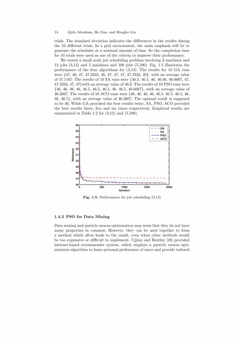
We tested a small scale job scheduling problem involving 3 machines and13 jobs (3,13) and 5 machines and 100 jobs (5,100). Fig. 1.5 illustrates theperformance of the four algorithms for (3,13). The results for 10 GA runswere {47, 46, 47, 47.3333, 46, 47, 47, 47, 47.3333, 49}, with an average valueof 47.1167. The results of 10 SA runs were {46.5, 46.5, 46, 46,46, 46.6667, 47,47.3333, 47, 47}with an average value of 46.6. The results of 10 PSO runs were{46, 46, 46, 46, 46.5, 46.5, 46.5, 46, 46.5, 46.6667}, with an average value of46.2667. The results of 10 ACO runs were {46, 46, 46, 46, 46.5, 46.5, 46.5, 46,46, 46.5}, with an average value of 46.2667. The optimal result is supposedto be 46. While GA provided the best results twice, SA, PSO, ACO providedthe best results three, five and six times respectively. Empirical results aresummarized in Table 1.2 for (3,13) and (5,100).
0 500 1000 1500 200046
47
48
49
50
51
52
53
54
55
56
Iteration
Mak
esp
an
GASAPSOACO
Fig. 1.5. Performance for job scheduling (3,13)
1.4.2 PSO for Data Mining
Data mining and particle swarm optimization may seem that they do not havemany properties in common. However, they can be used together to forma method which often leads to the result, even when other methods wouldbe too expensive or difficult to implement. Ujjinn and Bentley [28] providedinternet-based recommender system, which employs a particle swarm opti-mization algorithm to learn personal preferences of users and provide tailored
1 Swarm Intelligence: Foundations, Perspectives and Applications 15
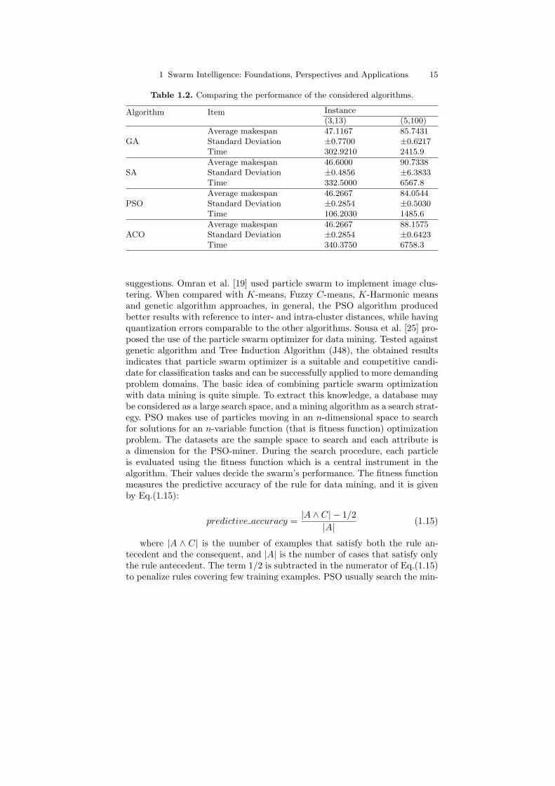
Table 1.2. Comparing the performance of the considered algorithms.
InstanceAlgorithm Item(3,13) (5,100)
Average makespan 47.1167 85.7431GA Standard Deviation ±0.7700 ±0.6217
Time 302.9210 2415.9
Average makespan 46.6000 90.7338SA Standard Deviation ±0.4856 ±6.3833
Time 332.5000 6567.8
Average makespan 46.2667 84.0544PSO Standard Deviation ±0.2854 ±0.5030
Time 106.2030 1485.6
Average makespan 46.2667 88.1575ACO Standard Deviation ±0.2854 ±0.6423
Time 340.3750 6758.3
suggestions. Omran et al. [19] used particle swarm to implement image clus-tering. When compared with K-means, Fuzzy C-means, K-Harmonic meansand genetic algorithm approaches, in general, the PSO algorithm producedbetter results with reference to inter- and intra-cluster distances, while havingquantization errors comparable to the other algorithms. Sousa et al. [25] pro-posed the use of the particle swarm optimizer for data mining. Tested againstgenetic algorithm and Tree Induction Algorithm (J48), the obtained resultsindicates that particle swarm optimizer is a suitable and competitive candi-date for classification tasks and can be successfully applied to more demandingproblem domains. The basic idea of combining particle swarm optimizationwith data mining is quite simple. To extract this knowledge, a database maybe considered as a large search space, and a mining algorithm as a search strat-egy. PSO makes use of particles moving in an n-dimensional space to searchfor solutions for an n-variable function (that is fitness function) optimizationproblem. The datasets are the sample space to search and each attribute isa dimension for the PSO-miner. During the search procedure, each particleis evaluated using the fitness function which is a central instrument in thealgorithm. Their values decide the swarm’s performance. The fitness functionmeasures the predictive accuracy of the rule for data mining, and it is givenby Eq.(1.15):
predictive accuracy =|A ∧ C| − 1/2
|A| (1.15)
where |A ∧ C| is the number of examples that satisfy both the rule an-tecedent and the consequent, and |A| is the number of cases that satisfy onlythe rule antecedent. The term 1/2 is subtracted in the numerator of Eq.(1.15)to penalize rules covering few training examples. PSO usually search the min-
16 Ajith Abraham, He Guo, and Hongbo Liu
imum for the problem space considered. So we use predictive accuracy to thepower minus one as fitness function in PSO-miner.
Rule pruning is a common technique in data mining. The main goal of rulepruning is to remove irrelevant terms that might have been unduly includedin the rules. Rule pruning potentially increases the predictive power of therule, helping to avoid its over-fitting to the training data. Another motivationfor rule pruning is that it improves the simplicity of the rule, since a shorterrule is usually easier to be understood by the user than a longer one. As soonas the current particle completes the construction of its rule, the rule pruningprocedure is called. The quality of a rule, denoted by Q, is computed by theformula: Q = sensitivity · specificity [17]. Just after the covering algorithmreturns a rule set, another post-processing routine is used: rule set cleaning,where rules that will never be applied are removed from the rule set. Thepurpose of the validation algorithm is to statistically evaluate the accuracy ofthe rule set obtained by the covering algorithm. This is done using a methodknown as tenfold cross validation [29]. Rule set accuracy is evaluated andpresented as the percentage of instances in the test set correctly classified. Inorder to classify a new test case, unseen during training, the discovered rulesare applied in the order they were discovered.
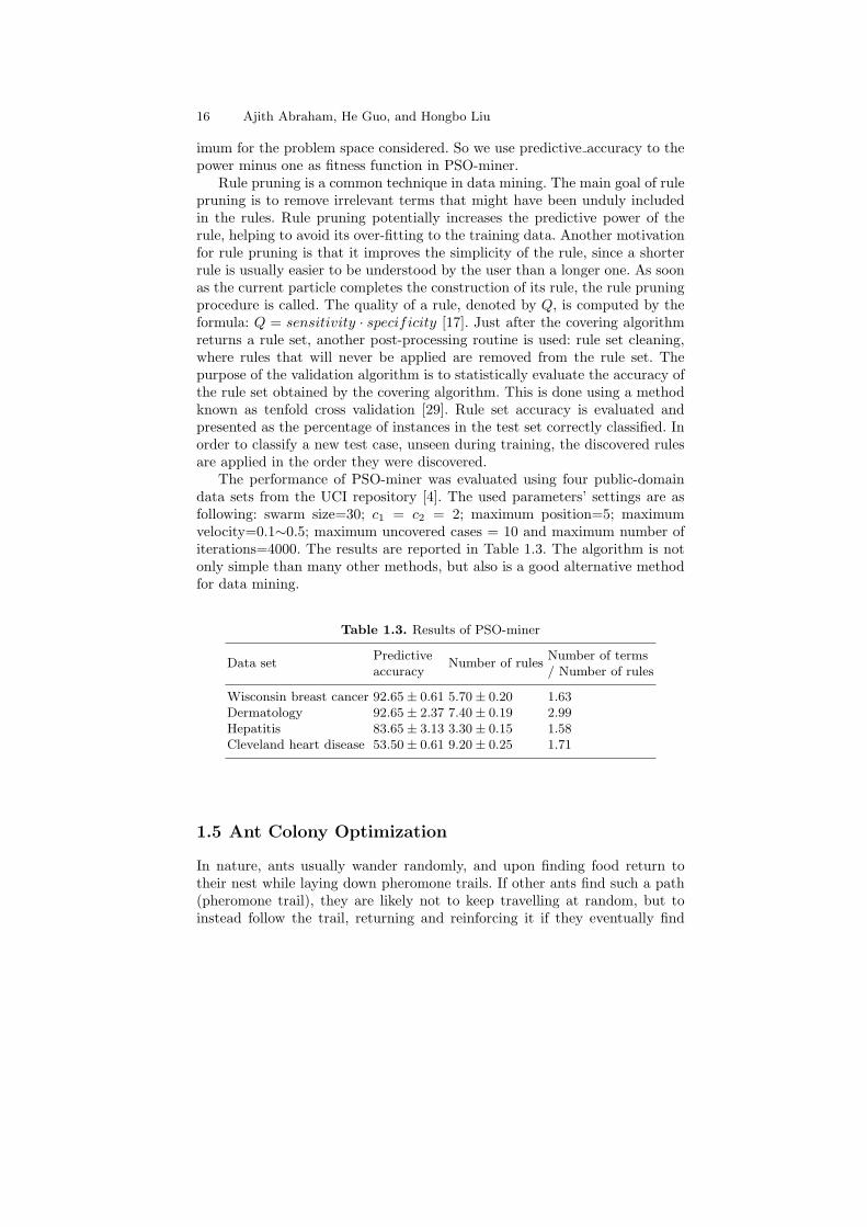
The performance of PSO-miner was evaluated using four public-domaindata sets from the UCI repository [4]. The used parameters’ settings are asfollowing: swarm size=30; c1 = c2 = 2; maximum position=5; maximumvelocity=0.1∼0.5; maximum uncovered cases = 10 and maximum number ofiterations=4000. The results are reported in Table 1.3. The algorithm is notonly simple than many other methods, but also is a good alternative methodfor data mining.
Table 1.3. Results of PSO-miner
Predictive Number of termsData set
accuracyNumber of rules
/ Number of rules
Wisconsin breast cancer 92.65 ± 0.61 5.70 ± 0.20 1.63Dermatology 92.65 ± 2.37 7.40 ± 0.19 2.99Hepatitis 83.65 ± 3.13 3.30 ± 0.15 1.58Cleveland heart disease 53.50 ± 0.61 9.20 ± 0.25 1.71
1.5 Ant Colony Optimization
In nature, ants usually wander randomly, and upon finding food return totheir nest while laying down pheromone trails. If other ants find such a path(pheromone trail), they are likely not to keep travelling at random, but toinstead follow the trail, returning and reinforcing it if they eventually find

1 Swarm Intelligence: Foundations, Perspectives and Applications 17
food. However, as time passes, the pheromone starts to evaporate. The moretime it takes for an ant to travel down the path and back again, the more timethe pheromone has to evaporate (and the path to become less prominent). Ashorter path, in comparison will be visited by more ants (can be described asa loop of positive feedback) and thus the pheromone density remains high fora longer time.
ACO is implemented as a team of intelligent agents which simulate theants behavior, walking around the graph representing the problem to solveusing mechanisms of cooperation and adaptation. ACO algorithm requires todefine the following [5, 10]:
• The problem needs to be represented appropriately, which would allow theants to incrementally update the solutions through the use of a probabilis-tic transition rules, based on the amount of pheromone in the trail andother problem specific knowledge. It is also important to enforce a strategyto construct only valid solutions corresponding to the problem definition.
• A problem-dependent heuristic function η that measures the quality ofcomponents that can be added to the current partial solution.
• A rule set for pheromone updating, which specifies how to modify thepheromone value τ .
• A probabilistic transition rule based on the value of the heuristic function ηand the pheromone value τ that is used to iteratively construct a solution.
ACO was first introduced using the Travelling Salesman Problem (TSP).Starting from its start node, an ant iteratively moves from one node to an-other. When being at a node, an ant chooses to go to a unvisited node at timet with a probability given by
pki,j(t) =
[τi,j(t)]α[ηi,j(t)]β∑l∈Nk
i[τi,j(t)]α[ηi,j(t)]β
j ∈ Nki (1.16)
where Nki is the feasible neighborhood of the antk, that is, the set of cities
which antk has not yet visited; τi,j(t) is the pheromone value on the edge(i, j) at the time t, α is the weight of pheromone; ηi,j(t) is a priori availableheuristic information on the edge (i, j) at the time t, β is the weight of heuris-tic information. Two parameters α and β determine the relative influence ofpheromone trail and heuristic information. τi,j(t) is determined by
τi,j(t) = ρτi,j(t − 1) +n∑
k=1
∆τki,j(t) ∀(i, j) (1.17)
∆τki,j(t) =
QLk(t) if the edge (i, j) chosen by the antk0 otherwise
(1.18)
where ρ is the pheromone trail evaporation rate (0 < ρ < 1), n is thenumber of ants, Q is a constant for pheromone updating.

18 Ajith Abraham, He Guo, and Hongbo Liu
More recent work has seen the application of ACO to other problems[12, 26]. A generalized version of the pseudo-code for the ACO algorithm withreference to the TSP is illustrated in Algorithm 2.
Algorithm 2 Ant Colony Optimization Algorithm01. Initialize the number of ants n, and other parameters.02. While (the end criterion is not met) do03. t = t + 1;04. For k= 1 to n05. antk is positioned on a starting node;06. For m= 2 to problem size07. Choose the state to move into08. according to the probabilistic transition rules;09. Append the chosen move into tabuk(t) for the antk;10. Next m11. Compute the length Lk(t) of the tour Tk(t) chosen by the antk;12. Compute ∆τi,j(t) for every edge (i, j) in Tk(t) according to Eq.(1.18);13. Next k14. Update the trail pheromone intensity for every edge (i, j) according toEq.(1.17);15. Compare and update the best solution;16. End While.
1.6 Ant Colony Algorithms for Optimization Problems
1.6.1 Travelling Salesman Problem (TSP)
Given a collection of cities and the cost of travel between each pair of them,the travelling salesman problem is to find the cheapest way of visiting all ofthe cities and returning to the starting point. It is assumed that the travelcosts are symmetric in the sense that travelling from city X to city Y costsjust as much as travelling from Y to X. The parameter settings used for ACOalgorithm are as follows:
Number of ants = 5Maximum number of iterations = 1000α = 2β = 2ρ = 0.9Q = 10
A TSP with 20 cities (Table 1.4) is used to illustrate the ACO algorithm.

1 Swarm Intelligence: Foundations, Perspectives and Applications 19
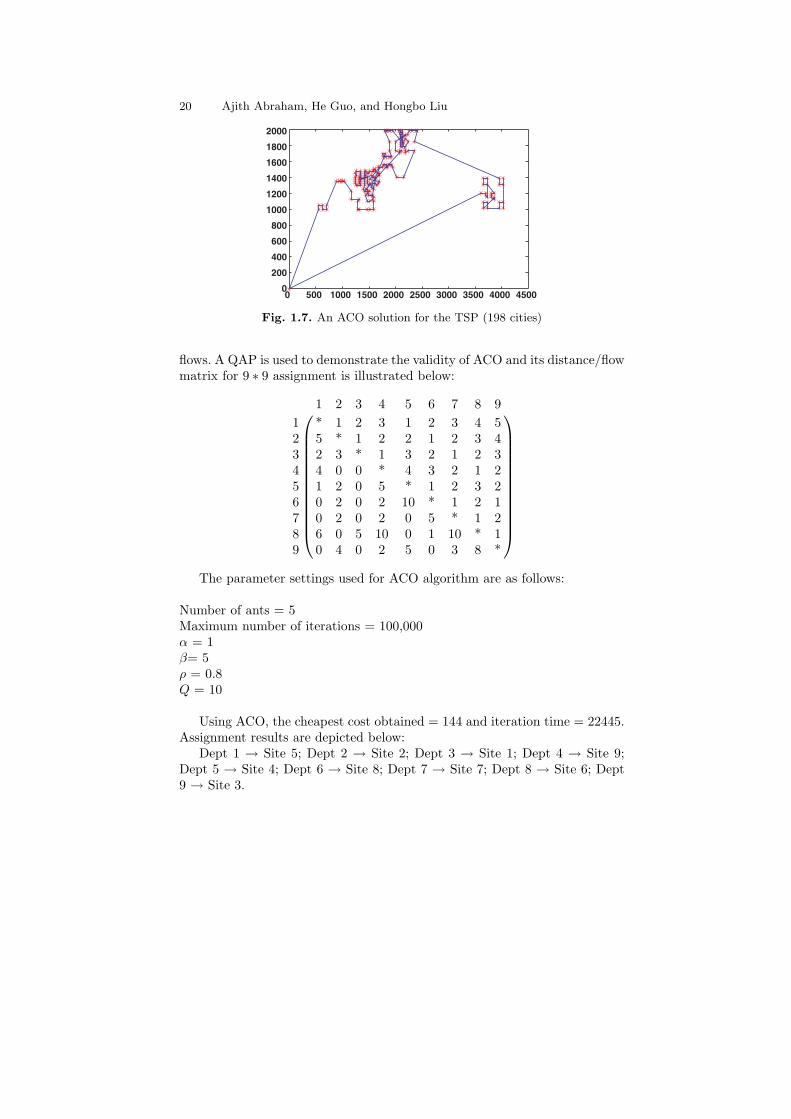
The best route obtained is depicted as 1 → 14 → 11 → 4 → 8 → 10 → 15 →19 → 7 → 18 → 16 → 5 → 13 → 20 → 6 → 17 → 9 → 2 → 12 → 3 → 1, andis illustrated in Fig. 1.6 with a cost of 24.5222. The search result for a TSPfor 198 cities is illustrated in Figure 1.7 with a total cost of 19961.3045.
Table 1.4. A TSP (20 cities)
Cities 1 2 3 4 5 6 7 8 9 10
x 5.2940 4.2860 4.7190 4.1850 0.9150 4.7710 1.5240 3.4470 3.7180 2.6490y 1.5580 3.6220 2.7740 2.2300 3.8210 6.0410 2.8710 2.1110 3.6650 2.5560
Cities 11 12 13 14 15 16 17 18 19 20
x 4.3990 4.6600 1.2320 5.0360 2.7100 1.0720 5.8550 0.1940 1.7620 2.6820y 1.1940 2.9490 6.4400 0.2440 3.1400 3.4540 6.2030 1.8620 2.6930 6.0970
0 1 2 3 4 5 60
1
2
3
4
5
6
7
Fig. 1.6. An ACO solution for the TSP (20 cities)
1.6.2 Quadratic Assignment Problem (QAP)
Quadratic assignment problems model many applications in diverse areas suchas operations research, parallel and distributed computing, and combinatorialdata analysis. There are a set of n facilities and a set of n locations. For eachpair of locations a distance is specified and for each pair of facilities a weightor flow is specified (e.g., the amount of supplies transported between the twofacilities). The problem is to assign all facilities to different locations with thegoal of minimizing the sum of the distances multiplied by the corresponding
20 Ajith Abraham, He Guo, and Hongbo Liu
0 500 1000 1500 2000 2500 3000 3500 4000 45000
200
400
600
800
1000
1200
1400
1600
1800
2000
Fig. 1.7. An ACO solution for the TSP (198 cities)
flows. A QAP is used to demonstrate the validity of ACO and its distance/flowmatrix for 9 ∗ 9 assignment is illustrated below:
⎛
⎜⎜⎜⎜⎜⎜⎜⎜⎜⎜⎜⎜⎝
1 2 3 4 5 6 7 8 91 * 1 2 3 1 2 3 4 52 5 * 1 2 2 1 2 3 43 2 3 * 1 3 2 1 2 34 4 0 0 * 4 3 2 1 25 1 2 0 5 * 1 2 3 26 0 2 0 2 10 * 1 2 17 0 2 0 2 0 5 * 1 28 6 0 5 10 0 1 10 * 19 0 4 0 2 5 0 3 8 *
⎞
⎟⎟⎟⎟⎟⎟⎟⎟⎟⎟⎟⎟⎠
The parameter settings used for ACO algorithm are as follows:
Number of ants = 5Maximum number of iterations = 100,000α = 1β= 5ρ = 0.8Q = 10
Using ACO, the cheapest cost obtained = 144 and iteration time = 22445.Assignment results are depicted below:
Dept 1 → Site 5; Dept 2 → Site 2; Dept 3 → Site 1; Dept 4 → Site 9;Dept 5 → Site 4; Dept 6 → Site 8; Dept 7 → Site 7; Dept 8 → Site 6; Dept9 → Site 3.
1 Swarm Intelligence: Foundations, Perspectives and Applications 21
1.7 Ant Colony Algorithms for Data Mining
The study of ant colonies behavior and their self-organizing capabilities is ofinterest to knowledge retrieval/management and decision support systems sci-ences, because it provides models of distributed adaptive organization, whichare useful to solve difficult classification, clustering and distributed controlproblems.
Ant colony based clustering algorithms have been first introduced byDeneubourg et al. [8] by mimicking different types of naturally-occurringemergent phenomena. Ants gather items to form heaps (clustering of deadcorpses or cemeteries) observed in the species of Pheidole Pallidula and La-sius Niger. If sufficiently large parts of corpses are randomly distributed inspace, the workers form cemetery clusters within a few hours, following abehavior similar to segregation. If the experimental arena is not sufficientlylarge, or if it contains spatial heterogeneities, the clusters will be formed alongthe edges of the arena or, more generally, following the heterogeneities. Thebasic mechanism underlying this type of aggregation phenomenon is an at-traction between dead items mediated by the ant workers: small clusters ofitems grow by attracting workers to deposit more items. It is this positiveand auto-catalytic feedback that leads to the formation of larger and largerclusters.
A sorting approach could be also formulated by mimicking ants that dis-criminate between different kinds of items and spatially arrange them accord-ing to their properties. This is observed in the Leptothorax unifasciatus specieswhere larvae are arranged according to their size.
The general idea for data clustering is that isolated items should be pickedup and dropped at some other location where more items of that type arepresent. Ramos et al. [23] proposed ACLUSTER algorithm to follow real ant-like behaviors as much as possible. In that sense, bio-inspired spatial transi-tion probabilities are incorporated into the system, avoiding randomly movingagents, which encourage the distributed algorithm to explore regions mani-festly without interest. The strategy allows guiding ants to find clusters ofobjects in an adaptive way.
In order to model the behavior of ants associated with different tasks(dropping and picking up objects), the use of combinations of different re-sponse thresholds was proposed. There are two major factors that should in-fluence any local action taken by the ant-like agent: the number of objects inits neighborhood, and their similarity. Lumer and Faieta [18] used an averagesimilarity, mixing distances between objects with their number, incorporatingit simultaneously into a response threshold function like the algorithm pro-posed by Deneubourg et al. [8]. ACLUSTER [23] uses combinations of twoindependent response threshold functions, each associated with a different en-vironmental factor depending on the number of objects in the area, and theirsimilarity. Reader may consult [23] for the technical details of ACLUSTER.

22 Ajith Abraham, He Guo, and Hongbo Liu
Fig. 1.8. Clustering of Web server visitors using ant colony algorithm (adaptedfrom [3])
1.7.1 Web Usage Mining
Web usage mining has become very critical for effective Web site management,creating adaptive Web sites, business and support services, personalization,network traffic flow analysis etc. [3]. Accurate Web usage information couldhelp to attract new customers, retain current customers, improve cross mar-keting/sales, effectiveness of promotional campaigns, track leaving customersand find the most effective logical structure for their Web space. User profilescould be built by combining users’ navigation paths with other data features,such as page viewing time, hyperlink structure, and page content.
Abraham and Ramos [3] used an ant colony clustering algorithm to dis-cover Web usage patterns (data clusters). The task is to cluster similar visitorsaccessing the web server based on geographical location, type of informationrequested, time of access and so on. Web log data of a University server fromJanuary 01, 2002 to July 0, 2002 was used in the experiments. The log datawas categorized into daily and hourly and for each data set the ACLUSTERwas run twice for 10,00,000 iterations. A 2D classification space is used whichis non-parametric and toroidal.
1 Swarm Intelligence: Foundations, Perspectives and Applications 23
Experiment results for the daily and hourly Web traffic data are illustratedin Fig. 1.8. Fig. 1.8, at the top, represent the spatial distribution of daily Webtraffic data on a 25×25 non-parametric toroidal grid. At t=1, data items arerandomly allocated and 14 ants were deployed and as time evolved, severalhomogenous clusters emerged. Figure 1.8, at the bottom, represent the spatialdistribution of hourly Web traffic data on a 45×45 non-parametric toroidalgrid. At t=1, data items are randomly allocated and 48 ants were deployed andas time evolved, several homogenous clusters emerged. Reader may consult [3]for detailed results of the different clustering methods.
Clustering results clearly show that ant colony clustering performs wellwhen compared to other clustering methods namely self-organizing maps andevolutionary-fuzzy clustering approach [1].
1.8 Summary
This chapter introduced the theoretical foundations of swarm intelligence witha focus on the implementation and illustration of particle swarm optimiza-tion and ant colony optimization algorithms. We provided the design and im-plementation methods for some applications involving function optimizationproblems, real world applications and data mining. Results were analyzed,discussed and their potentials were illustrated.
Acknowledgements
First author was supported by the International Joint Research Grant of theIITA (Institute of Information Technology Assessment) foreign professor in-vitation program of the MIC (Ministry of Information and Communication),South Korea.
References
1. Abraham A (2003) Business intelligence from web usage mining, Journal ofInformation and Knowledge Management (JIKM), World Scientific PublishingCo., Singapore, 2(4)375-390.
2. Abraham A, Buyya R and Nath B (2000) Nature’s heuristics for scheduling jobson computational grids. Proceedings of the 8th IEEE International Conferenceon Advanced Computing and Communications, 45-52.
3. Abraham A and Ramos V (2003) Web usage mining using artificial ant colonyclustering and genetic programming. Proceesings of IEEE Congress on Evolu-tionary Computation, Australia, 1384-1391.
4. Blake C, Keogh E and Merz C J (2003) UCI repository of machine learningdatabases. http://ww.ic.uci.edu/ mlearn/MLRepository.htm.
24 Ajith Abraham, He Guo, and Hongbo Liu
5. Bonabeau E, Dorigo M and Theraulaz G (1999) Swarm Intelligence: From Nat-ural to Artificial Systems. New York, NY: Oxford University Press.
6. Cantu-Paz E (2000) Efficient and Accurate Parallel Genetic Algorithms. KluwerAcademic publishers.
7. Clerc M and Kennedy J (2002) The particle swarm-explosion, stability, andconvergence in a multidimensional complex space. IEEE Transactions on Evo-lutionary Computation, 6(1):58-73.
8. Deneubourg J-L, Goss S, Franks N, at el. (1991) The dynamics of collective sort-ing: Robot-like ants and ant-like robots. Proceedings of the First InternationalConference on Simulation of Adaptive Behaviour: From Animals to Animats,Cambridge, MA: MIT Press, 1, 356-365.
9. Dorigo M, Maniezzo V and Colorni A (1996). Ant system: optimization bya colony of cooperating agents. IEEE Transactions on Systems, Man, andCybernetics-Part B, 26(1):29-41.
10. Dorigo M and Stutzle T (2004), Ant Colony Optimization, MIT Press, 2004.11. Eberhart R C and Shi Y (2002) Comparing inertia weights and constriction fac-
tors in particle swarm optimization. Proceedings of IEEE International Congresson Evolutionary Computation, 84-88.
12. Gambardella L M and Dorigo M (1995) Ant-Q: A reinforcement learning ap-proach to the traveling salesman problem. Proceedings of the 11th InternationalConference on Machine Learning, 252-260.
13. Goldberg D E (1989) Genetic Algorithms in search, optimization, and machinelearning. Addison-Wesley Publishing Corporation, Inc.
14. Kennedy J and Eberhart R (2001) Swarm intelligence. Morgan Kaufmann Pub-lishers, Inc., San Francisco, CA.
15. Kennedy J and Mendes R (2002) Population structure and particle swarm per-formance. Proceeding of IEEE conference on Evolutionary Computation, 1671-1676.
16. Liu H and Abraham A (2005) Fuzzy Turbulent Particle Swarm Optimization.Proceeding of the 5th International Conference on Hybrid Intelligent Systems,Brazil, IEEE CS Press, USA.
17. Lopes H S, Coutinho M S and Lima W C (1998) An evolutionary approach tosimulate cognitive feedback learning in medical domain. Genetic Algorithms andFuzzy Logic Systems: Soft Computing Perspectives, World Scientific, 193-207.
18. Lumer E D and Faieta B (1994) Diversity and Adaptation in Populations ofClustering Ants. Cli D, Husbands P, Meyer J and Wilson S (Eds.), Proceedingsof the Third International Conference on Simulation of Adaptive Behaviour:From Animals to Animats 3, Cambridge, MA: MIT Press, 501-508.
19. Omran M, Engelbrecht P A and Salman A (2005) Particle swarm optimizationfor image clustering. International Journal of Pattern Recognition and ArtificialIntelligence, 19(3):297-321.
20. Orosz J E and Jacobson S H (2002) Analysis of static simulated annealingalgorithms. Journal of Optimzation theory and Applications, 115(1):165-182.
21. Pang W, Wang K P, Zhou C G, at el. (2004) Fuzzy discrete particle swarmoptimization for solving traveling salesman problem. Proceedings of the 4thInternational Conference on Computer and Information Technology, IEEE CSPress.
22. Parsopoulos K E and Vrahatis M N (2004) On the computation of all globalminimizers through particle swarm optimization. IEEE Transactions on Evolu-tionary Computation, 8(3):211-224.
1 Swarm Intelligence: Foundations, Perspectives and Applications 25
23. Ramos V, Muge F, Pina P (2002) Self-organized data and image retrieval as aconsequence of inter-dynamic synergistic relationships in artificial ant colonies.Soft Computing Systems - Design, Management and Applications, Proceedingsof the 2nd International Conference on Hybrid Intelligent Systems, IOS Press,500-509.
24. Shi Y H and Eberhart R C (2001) Fuzzy adaptive particle swarm optimization.Proceedings of IEEE International Conference on Evolutionary Computation,101-106.
25. Sousa T, Silva A, Neves A (2004) Particle swarm based data mining algorithmsfor classification tasks. Parallel Computing, 30:767-783.
26. Stutzle T and Hoo H H (2000) MAX-MIN ant system. Future Generation Com-puter Systems, 16:889-914.
27. Triki E, Collette Y and Siarry P (2005) A theoretical study on the behaviorof simulated annealing leading to a new cooling schedule. European Journal ofOperational Research, 166:77-92.
28. Ujjin S and Bentley J P (2003) Particle swarm optimization recommender sys-tem. Proceeding of IEEE International conference on Evolutionary Computa-tion, 124-131.
29. Witten Ian H and Frank E (1999) Data mining - Practical Machine LearningTools and Techniques with Java Implementations. CA: Morgan Kauffmann.