Embed Size (px)
Citation preview
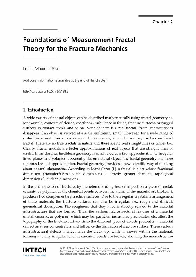
Chapter 2
© 2012 Alves, licensee InTech. This is an open access chapter distributed under the terms of the Creative Commons Attribution License (http://creativecommons.org/licenses/by/3.0), which permits unrestricted use, distribution, and reproduction in any medium, provided the original work is properly cited.
Foundations of Measurement Fractal Theory for the Fracture Mechanics
Lucas Máximo Alves
Additional information is available at the end of the chapter
http://dx.doi.org/10.5772/51813
1. Introduction
A wide variety of natural objects can be described mathematically using fractal geometry as, for example, contours of clouds, coastlines , turbulence in fluids, fracture surfaces, or rugged surfaces in contact, rocks, and so on. None of them is a real fractal, fractal characteristics disappear if an object is viewed at a scale sufficiently small. However, for a wide range of scales the natural objects look very much like fractals, in which case they can be considered fractal. There are no true fractals in nature and there are no real straight lines or circles too. Clearly, fractal models are better approximations of real objects that are straight lines or circles. If the classical Euclidean geometry is considered as a first approximation to irregular lines, planes and volumes, apparently flat on natural objects the fractal geometry is a more rigorous level of approximation. Fractal geometry provides a new scientific way of thinking about natural phenomena. According to Mandelbrot [1], a fractal is a set whose fractional dimension (Hausdorff-Besicovitch dimension) is strictly greater than its topological dimension (Euclidean dimension).
In the phenomenon of fracture, by monotonic loading test or impact on a piece of metal, ceramic, or polymer, as the chemical bonds between the atoms of the material are broken, it produces two complementary fracture surfaces. Due to the irregular crystalline arrangement of these materials the fracture surfaces can also be irregular, i.e., rough and difficult geometrical description. The roughness that they have is directly related to the material microstructure that are formed. Thus, the various microstructural features of a material (metal, ceramic, or polymer) which may be, particles, inclusions, precipitates, etc. affect the topography of the fracture surface, since the different types of defects present in a material can act as stress concentrators and influence the formation of fracture surface. These various microstructural defects interact with the crack tip, while it moves within the material, forming a totally irregular relief as chemical bonds are broken, allowing the microstructure
Applied Fracture Mechanics 20
to be separated from grains (transgranular and intergranular fracture) and microvoids are joining (coalescence of microvoids, etc..) until the fracture surfaces depart. Moreover, the characteristics of macrostructures such as the size and shape of the sample and notch from which the fracture is initiated, also influence the formation of the fracture surface, due to the type of test and the stress field applied to the specimen.
After the above considerations, one can say with certainty that the information in the fracture process are partly recorded in the "story" that describes the crack, as it walks inside the material [2]. The remainder of this information is lost to the external environment in a form of dissipated energy such as sound, heat, radiation, etc. [30, 31]. The remaining part of the information is undoubtedly related to the relief of the fracture surface that somehow describes the difficulty that the crack found to grow [2]. With this, you can analyze the fracture phenomenon through the relief described by the fracture surface and try to relate it to the magnitudes of fracture mechanics [3 , 4 , 5 , 6 , 7, 8, 9 - 11, 12, 13]. This was the basic idea that brought about the development of the topographic study of the fracture surface called fractography.
In fractography anterior the fractal theory the description of geometric structures found on a fracture surface was limited to regular polyhedra-connected to each other and randomly distributed throughout fracture surface, as a way of describing the topography of the irregular surface. Moreover, the study fractographic hitherto used only techniques and statistical analysis profilometric relief without considering the geometric auto-correlation of surfaces associated with the fractal exponents that characterize the roughness of the fracture surface.
The basic concepts of fractal theory developed by Mandelbrot [1] and other scientists, have been used in the description of irregular structures, such as fracture surfaces and crack [14 ], in order to relate the geometrical description of these objects with the materials properties [15 ].
The fractal theory, from the viewpoint of physical, involves the study of irregular structures which have the property of invariance by scale transformation, this property in which the parts of a structure are similar to the whole in successive ranges of view (magnification or reduction) in all directions or at least one direction (self-similarity or self-affinity, respectively) [36]. The nature of these intriguing properties in existing structures, which extend in several scales of magnification is the subject of much research in several phenomena in nature and in materials science [16 , 17 and others]. Thus, the fractal theory has many contexts, both in physics and in mathematics such as chaos theory [18], the study of phase transitions and critical phenomena [19, 20, 21], study of particle agglomeration [22], etc.. The context that is more directly related to Fracture Mechanics, because of the physical nature of the process is with respect to fractal growth [23, 24, 25, 26]. In this subarea are studied the growth mechanisms of structures that arise in cases of instability, and dissipation of energy, such as crack [27, 28] and branching patterns [29]. In this sense, is to be sought to approach the problem of propagation of cracks.
Foundations of Measurement Fractal Theory for the Fracture Mechanics 21
The fractal theory becomes increasingly present in the description of phenomena that have a measurable disorder, called deterministic chaos [18, 27, 28]. The phenomenon of fracture and crack propagation, while being statistically shows that some rules or laws are obeyed, and every day become more clear or obvious, by understanding the properties of fractals [27, 28].
2. Fundamental geometric elements and measure theory on fractal geometry
In this part will be presented the development of basic concepts of fractal geometry, analogous to Euclidean geometry for the basic elements such as points, lines, surfaces and fractals volumes. It will be introduce the measurement fractal theory as a generalization of Euclidean measure geometric theory. It will be also describe what are the main mathematical conditions to obtain a measure with fractal precision.
2.1. Analogy between euclidean and fractal geometry
It is possible to draw a parallel between Euclidean and fractal geometry showing some examples of self-similar fractals projected onto Euclidean dimensions and some self-affine fractals. For, just as in Euclidean geometry, one has the elements of geometric construction, in the fractal geometry. In the fractal geometry one can find similar objects to these Euclidean elements. The different types of fractals that exist are outlined in Figure 1 to Figure 4.
2.1.1. Fractais between 0 1D (similar to point)
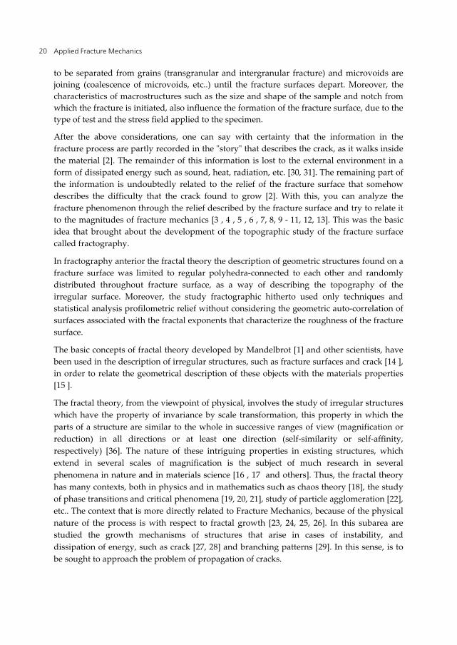
An example of a fractal immersed in Euclidean dimension 1 1I d with projection in 0d , similar to punctiform geometry, can be exemplified by the Figure 1.
Figure 1. Fractal immersed in the one-dimensional space where 0,631D .
This fractal has dimension 0,631D . This is a fractal-type "stains on the floor." Other fractal of this type can be observed when a material is sprayed onto a surface. In this case the global dimension of the spots may be of some value between 0 1D .
2.1.2. Fractais between 1 2D (similar to straight lines)
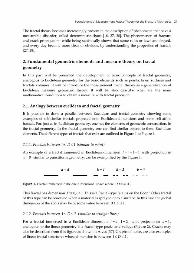
For a fractal immersed in a Euclidean dimension 1 2I d , with projectionin 1d , analogous to the linear geometry is a fractal-type peaks and valleys (Figure 2). Cracks may also be described from this figure as shown in Alves [37]. Graphs of noise, are also examples of linear fractal structures whose dimension is between 1 2D .
Applied Fracture Mechanics 22
Figure 2. Fractal immersed in dimension d = 2. rugged fractal line.
2.1.3. Fractals between 2 3D (similar to surfaces or porous volumes)
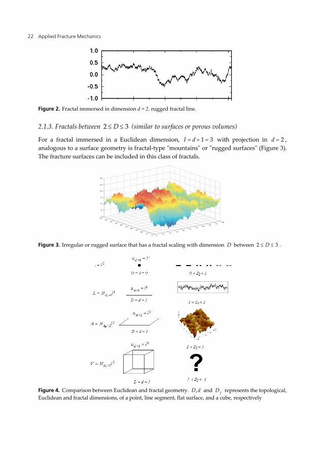
For a fractal immersed in a Euclidean dimension, 1 3I d with projection in 2d , analogous to a surface geometry is fractal-type "mountains" or "rugged surfaces" (Figure 3). The fracture surfaces can be included in this class of fractals.
Figure 3. Irregular or rugged surface that has a fractal scaling with dimension D between 2 3D .
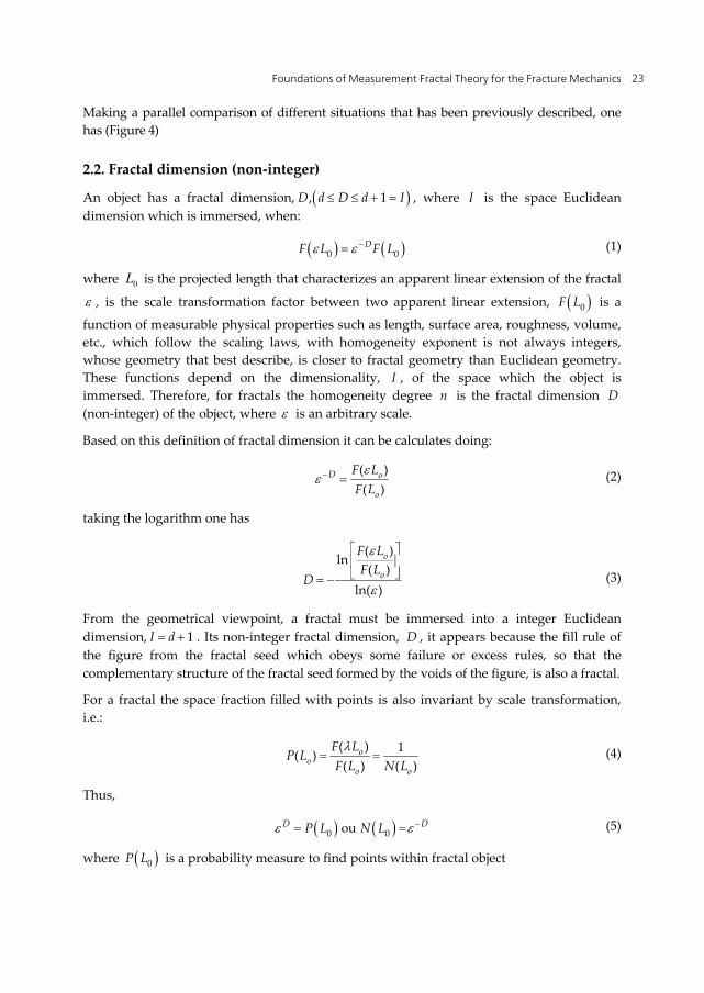
Figure 4. Comparison between Euclidean and fractal geometry. ,D d and fD represents the topological, Euclidean and fractal dimensions, of a point, line segment, flat surface, and a cube, respectively
Foundations of Measurement Fractal Theory for the Fracture Mechanics 23
Making a parallel comparison of different situations that has been previously described, one has (Figure 4)
2.2. Fractal dimension (non-integer)
An object has a fractal dimension, , 1D d D d I , where I is the space Euclidean dimension which is immersed, when:
0 0DF L F L (1)
where 0L is the projected length that characterizes an apparent linear extension of the fractal
, is the scale transformation factor between two apparent linear extension, 0F L is a
function of measurable physical properties such as length, surface area, roughness, volume, etc., which follow the scaling laws, with homogeneity exponent is not always integers, whose geometry that best describe, is closer to fractal geometry than Euclidean geometry. These functions depend on the dimensionality, I , of the space which the object is immersed. Therefore, for fractals the homogeneity degree n is the fractal dimension D (non-integer) of the object, where is an arbitrary scale.
Based on this definition of fractal dimension it can be calculates doing:
( )( )
D o
o
F LF L
(2)
taking the logarithm one has
( )ln
( )ln( )
o
o
F LF L
D
(3)
From the geometrical viewpoint, a fractal must be immersed into a integer Euclidean dimension, 1I d . Its non-integer fractal dimension, D , it appears because the fill rule of the figure from the fractal seed which obeys some failure or excess rules, so that the complementary structure of the fractal seed formed by the voids of the figure, is also a fractal.
For a fractal the space fraction filled with points is also invariant by scale transformation, i.e.:
( ) 1( )( ) ( )
oo
o o
F LP L
F L N L
(4)
Thus,
0 0ouD DP L N L (5)
where 0P L is a probability measure to find points within fractal object
Applied Fracture Mechanics 24
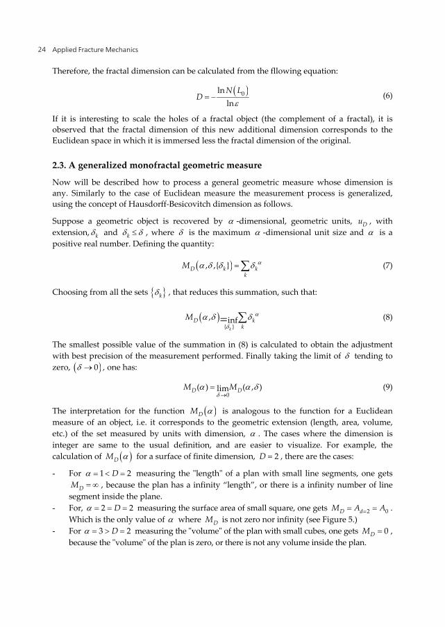
Therefore, the fractal dimension can be calculated from the fllowing equation:
0lnlnN L
D
(6)
If it is interesting to scale the holes of a fractal object (the complement of a fractal), it is observed that the fractal dimension of this new additional dimension corresponds to the Euclidean space in which it is immersed less the fractal dimension of the original.
2.3. A generalized monofractal geometric measure
Now will be described how to process a general geometric measure whose dimension is any. Similarly to the case of Euclidean measure the measurement process is generalized, using the concept of Hausdorff-Besicovitch dimension as follows.
Suppose a geometric object is recovered by -dimensional, geometric units, Du , with extension, k and k , where is the maximum -dimensional unit size and is a positive real number. Defining the quantity:
, ,{ }D k kk
M (7)
Choosing from all the sets k , that reduces this summation, such that:
{ }
, infk
D kk
M
(8)
The smallest possible value of the summation in (8) is calculated to obtain the adjustment with best precision of the measurement performed. Finally taking the limit of tending to zero, 0 , one has:
0
( ) ( , )limD DM M
(9)
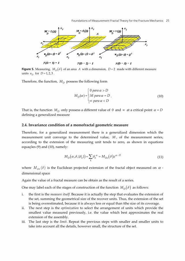
The interpretation for the function DM is analogous to the function for a Euclidean measure of an object, i.e. it corresponds to the geometric extension (length, area, volume, etc.) of the set measured by units with dimension, . The cases where the dimension is integer are same to the usual definition, and are easier to visualize. For example, the calculation of DM for a surface of finite dimension, 2D , there are the cases:
- For 1 2D measuring the "length" of a plan with small line segments, one gets
DM , because the plan has a infinity “length”, or there is a infinity number of line segment inside the plane.
- For, 2 2D measuring the surface area of small square, one gets 2 0D dM A A . Which is the only value of where DM is not zero nor infinity (see Figure 5.)
- For 3 2D measuring the "volume" of the plan with small cubes, one gets 0DM , because the "volume" of the plan is zero, or there is not any volume inside the plan.
Foundations of Measurement Fractal Theory for the Fracture Mechanics 25
Figure 5. Measuring, DM of an area A with a dimension, 2D made with different measure units Du for 1,2,3D .
Therefore, the function, DM possess the following form
0
( )D
para DM M para D
para D
. (10)
That is, the function DM only possess a different value of 0 and at a critical point D defining a generalized measure
2.4. Invariance condition of a monofractal geometric measure
Therefore, for a generalized measurement there is a generalized dimension which the measurement unit converge to the determined value, M , of the measurement series, according to the extension of the measuring unit tends to zero, as shown in equations equações (9) and (10), namely:
, ,{ } DD k k Do
kM M (11)
where ( )0DM d is the Euclidean projected extension of the fractal object measured on -dimensional space
Again the value of a fractal measure can be obtain as the result of a series.
One may label each of the stages of construction of the function DM as follows:
i. the first is the measure itself. Because it is actually the step that evaluates the extension of the set, summing the geometrical size of the recover units. Thus, the extension of the set is being overestimated, because it is always less or equal than tthe size of its coverage.
ii. The next step is the optimization to select the arrangement of units which provide the smallest value measured previously, i.e. the value which best approximates the real extension of the assembly.
iii. The last step is the limit. Repeat the previous steps with smaller and smaller units to take into account all the details, however small, the structure of the set.
Applied Fracture Mechanics 26
As the value of the generalized dimension is defined as a critical function, DM it can be concluded, wrongly, that the optimization step is not very important, because the fact of not having all its length measured accurately should not affect the value of critical point. The optimization step, this definition, serves to make the convergence to go faster in following step, that the mathematical point of view is a very desirable property when it comes to numerical calculation algorithms.
2.5. The monofractal measure and the Hausdorff-Besicovitch dimension
In this part we will define the dimension-Hausdorf Besicovicth and a fractal object itself. The basic properties of objects with "anomalous" dimensions (different from Euclidean) were observed and investigated at the beginning of this century, mainly by Hausdorff and Besicovitch [32,34]. The importance of fractals to physics and many other fields of knowledge has been pointed out by Mandelbrot [1]. He demonstrated the richness of fractal geometry, and also important results presented in his books on the subject [1, 35, 36].
The geometric sequence, S is given by:
0,1,2,....kk
S S onde k (12)
represented in Euclidean space, is a fractal when the measure of its geometric extension, given by the series, kM satisfies the following Hausdorf-Besicovitch condition:
0
0;( ) ( ) ( ) ( ) ;
;k
d k k d k k Dk
DM d N d M D
D
, (13)
where: d is the geometric factor of the unitary elements (or seed) of the sequence represented
geometrically. : is the size of unit elements (or seed), used as a measure standard unit of the extent of the spatial representation of the geometric sequence.
N : is the number of elementary units (or seeds) that form the spatial representation of the sequence at a certain scale : the generalized dimension of unitary elements D : is the Hausdorff-Besicovitch dimension.
2.6. Fractal mathematical definition and associated dimensions
Therefore, fractal is any object that has a non-integer dimension that exceeds the topological dimension ( D I , where I is the dimension of Euclidean space which is immersed) with some invariance by scale transformation (self-similarity or self-affinity), where for any continuous contour that is taken as close as possible to the object, the number of points DN , forming the fractal not fills completely the space delimited by the contour, i.e., there is
Foundations of Measurement Fractal Theory for the Fracture Mechanics 27
always empty, or excess regions, and also there is always a figure with integer dimension, I, at which the fractal can be inscribed and that not exactly superimposed on fractal even in the limit of scale infinitesimal. Therefore, the fraction of points that fills the fractal regarding its Euclidean coverage is different of a integer. As seen in previous sections - 2.2 - 2.5 in algebraic language, a fractal is a invariant sequence by scale transformation that has a Hausdorff-Besicovitch dimension.
According to the previous section, it is said that an object is fractal, when the respective magnitudes characterizing features as perimeter, area or volume, are homogeneous functions with non-integer. In this case, the invariance property by scaling transformation (self-similar or self-affinity) is due to a scale transformation of at least one of these functions.
The fractal concept is closely associated to the concept of Hausdorff-Besicovitch dimension, so that one of the first definitions of fractal created by Mandelbrot [36] was:
“Fractal by definition is a set to which the Haussdorf-Besicovitch dimension exceeds strictly the topological dimension".
One can therefore say that fractals are geometrical objects that have structures in all scales of magnification, commonly with some similarity between them. They are objects whose usual definition of Euclidean dimension is incomplete, requiring a more suitable to their context as they have just seen. This is exactly the Hausdorff-Besicovitch dimension.
A dimension object, D , is always immersed in a space of minimal dimension 1I d , which may present an excessive extension on the dimension d , or a lack of extension or failures in one dimension 1d . For example, for a crack which the fractal dimension is the dimension in the range of 1 2D the immersion dimension is the dimension 2I in the case of a fracture surface of which the fractal dimension is in the range 2 3D the immersion dimension is the 3I . When an object has a geometric extension such as completely fill a Euclidean dimension regular, d , and still have an excess that partially fills a superior dimension 1I d , in addition to the inferior dimension, one says that the object has a dimension in excess, ed given by ed D d where D is the dimension of the object. For example, for a crack which the fractal dimension is in the range 1 2D the excess dimension is 1ed D , in the case of a fracture surface of which the fractal dimension is in the range of 2 3D the excess dimension is 2ed D . If on the other hand an object partially fills a Euclidean regular dimension, 1I d certainly this object fills fully a Euclidean regular dimension, d , so that it is said that this object has a lack dimension
1fld I D d D , where 1e fld d . For example, for a crack which the fractal dimension is the range of 1 2D the lack dimension is 2fld D . In the case of a fracture surface of which the fractal dimension is the range of 2 3D the lack dimension is 3fld D .
2.7. Classes and types of fractals
One of the most fascinating aspects of the fractals is the extremely rich variety of possible realizations of such geometric objects. This fact gives rise to the question of classification,
Applied Fracture Mechanics 28
and the book of Mandelbrot [1] and in the following publications many types of fractal structures have been described. Below some important classes will be discussed with some emphasis on their relevance to the phenomenon of growth.
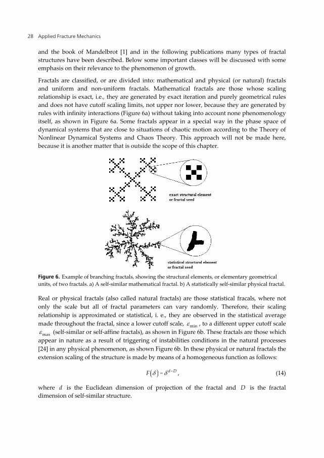
Fractals are classified, or are divided into: mathematical and physical (or natural) fractals and uniform and non-uniform fractals. Mathematical fractals are those whose scaling relationship is exact, i.e., they are generated by exact iteration and purely geometrical rules and does not have cutoff scaling limits, not upper nor lower, because they are generated by rules with infinity interactions (Figure 6a) without taking into account none phenomenology itself, as shown in Figure 6a. Some fractals appear in a special way in the phase space of dynamical systems that are close to situations of chaotic motion according to the Theory of Nonlinear Dynamical Systems and Chaos Theory. This approach will not be made here, because it is another matter that is outside the scope of this chapter.
Figure 6. Example of branching fractals, showing the structural elements, or elementary geometrical units, of two fractals. a) A self-similar mathematical fractal. b) A statistically self-similar physical fractal.
Real or physical fractals (also called natural fractals) are those statistical fracals, where not only the scale but all of fractal parameters can vary randomly. Therefore, their scaling relationship is approximated or statistical, i. e., they are observed in the statistical average made throughout the fractal, since a lower cutoff scale, min , to a different upper cutoff scale
max (self-similar or self-affine fractals), as shown in Figure 6b. These fractals are those which appear in nature as a result of triggering of instabilities conditions in the natural processes [24] in any physical phenomenon, as shown Figure 6b. In these physical or natural fractals the extension scaling of the structure is made by means of a homogeneous function as follows:
~ d DF , (14)
where d is the Euclidean dimension of projection of the fractal and D is the fractal dimension of self-similar structure.
Foundations of Measurement Fractal Theory for the Fracture Mechanics 29
It is true that the physical or real fractals can be deterministic or random. In random or statistical fractal the properties of self-similarity changes statistically from region to region of the fractal. The dimension cannot be unique, but characterized by a mean value, similarly to the analysis of mathematical fractals. The Figure 6b shows aspects of a statistically self-similar fractal whose appearance varies from branch to branch giving us the impression that each part is similar to the whole.
The mathematical fractals (or exact) and physical (or statistical), in turn, can be subdivided into uniform and nonuniform fractal.
Uniforms fractals are those that grow uniformly with a well behaved unique scale and constant factor, , and present a unique fractal dimension throughout its extension.
Non-uniform fractals are those that grow with scale factors 'i s that vary from region to region of the fractal and have different fractal dimensions along its extension.
Thus, the fractal theory can be studied under three fundamental aspects of its origin:
1. From the geometric patterns with self-similar features in different objects found in nature. 2. From the nonlinear dynamics theory in the phase space of complex systems. 3. From the geometric interpretation of the theory of critical exponents of statistical
mechanics.
3. Methods for measuring length, area, volume and fractal dimension
In this section one intends to describe the main methods for measuring the fractal dimension of a structure, such as: the compass method, the Box-Counting method, the Sand-Box Method, etc.
It will be described, from now, how to obtain a measure of length, area or fractal volume. In fractal analysis of an object or structure different types of fractal dimension are obtained, all related to the type of phenomenon that has fractality and the measurement method used in obtaining the fractal measurement. These fractal dimensions can be defined as follows.
3.1. The different fractal dimensions and its definitions
A fractal dimension fD in general is defined as being the dimension of the resulting measure of an object or structure, that has irregularities that are repeated in different scales (a invariance by scale transformation). Their values are usually noninteger and situated between two consecutive Euclidean dimensions called projection dimension d of the object and immersion dimension, 1d , i.e. 1fd D d .
In the literature there is controversy concerning the relationship between different fractal dimensions and roughness exponents. The term "fractal dimension" is used generically to refer to different fractional dimensions found in different phenomenologies, which results in formation of geometric patterns or energy dissipation, which are commonly called fractals [1]. Among these patterns is the growth of aggregates by diffusion (DLA - Diffusion Limited
Applied Fracture Mechanics 30
Aggregation), the film growth by ballistic deposition (BD), the fracture surfaces (SF), etc.. The fractal dimensions found in these phenomena are certainly not the same and depend on both the phenomenology studied as the fractal characterization method used. Therefore, to characterize such phenomena using fractal geometry, a distinction between the different dimensions found is necessary.
Among the various fractal dimensions one can emphasize the Hausdorff-Besicovitch dimension, HBD , which comes from the general mathematical definition of a fractal [32, 33,34]. Other dimensions are the dimension box, BD , the roughness dimension or exponent Hurst, H , the Lipshitz-Hölder dimension, , etc.. Therefore, a mathematical relationship between them needs to be clearly established for each phenomenon involved. However, is observed, then that relationship is not unique and depends not only on phenomenology, but also the characterization method used.
Therefore, the phenomenological equation of the fracture phenomenon can also, in theory, provide a relationship between fractal dimension and roughness exponent of a fracture surface, as happens to other phenomenologies. In this study, there was obtained a fractal model for a fracture surface, as a generalization of the box-counting method. Thus, will be discussed the relationship between the local and global box dimension and the roughness dimension, which are involved in the characterization of a fracture surface, and any other dimension necessary to describe a fractal fracture surface.
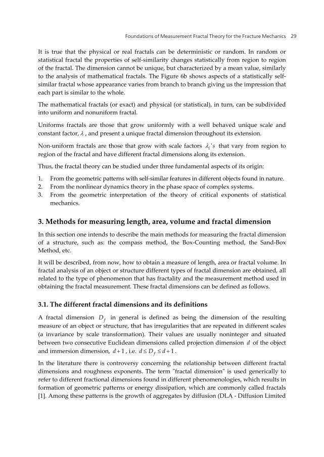
3.1.1. Compass methods and divider dimension, DD
The divider dimension DD is defined from the measure of length of a roughened fractal line, for example, when using the compass method. This measure is obtained by opening a compass with an aperture and moving on the line fractal to obtain the value of the line length rugosa (see Figure 7). The different values of the rough line length due to the compass aperture determines the dimension divider.
Figure 7. Compass method applied to a rugged line.
For a fractal rough line the divider dimension can be defined as:
Foundations of Measurement Fractal Theory for the Fracture Mechanics 31
0
ln
lnD
L
D
L
. (15)
where 0L is the projected length obtained from the rugged fractal length L
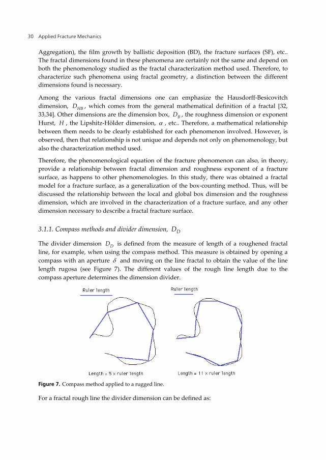
Figure 8. Compass method applied on a line noise or a rough self-affine fractal.
Several methods for determining the fractal dimension based on the compass method, among them stand out the following methods: the Coastlines Richardson Method, the Slit Island Method, etc.
3.2. Methods of measurement for determining the fractal dimension of a structure
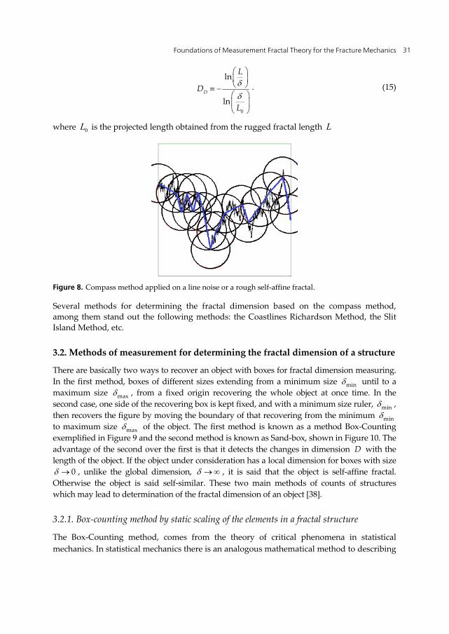
There are basically two ways to recover an object with boxes for fractal dimension measuring. In the first method, boxes of different sizes extending from a minimum size min until to a maximum size max , from a fixed origin recovering the whole object at once time. In the second case, one side of the recovering box is kept fixed, and with a minimum size ruler, min , then recovers the figure by moving the boundary of that recovering from the minimum min to maximum size max of the object. The first method is known as a method Box-Counting exemplified in Figure 9 and the second method is known as Sand-box, shown in Figure 10. The advantage of the second over the first is that it detects the changes in dimension D with the length of the object. If the object under consideration has a local dimension for boxes with size
0 , unlike the global dimension, , it is said that the object is self-affine fractal. Otherwise the object is said self-similar. These two main methods of counts of structures which may lead to determination of the fractal dimension of an object [38].
3.2.1. Box-counting method by static scaling of the elements in a fractal structure
The Box-Counting method, comes from the theory of critical phenomena in statistical mechanics. In statistical mechanics there is an analogous mathematical method to describing
Applied Fracture Mechanics 32
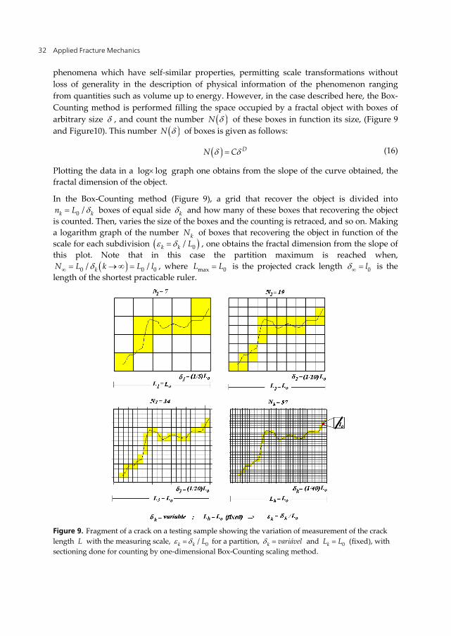
phenomena which have self-similar properties, permitting scale transformations without loss of generality in the description of physical information of the phenomenon ranging from quantities such as volume up to energy. However, in the case described here, the Box-Counting method is performed filling the space occupied by a fractal object with boxes of arbitrary size , and count the number N of these boxes in function its size, (Figure 9 and Figure10). This number N of boxes is given as follows:
DN C (16)
Plotting the data in a log log graph one obtains from the slope of the curve obtained, the fractal dimension of the object.
In the Box-Counting method (Figure 9), a grid that recover the object is divided into 0 /k kn L boxes of equal side k and how many of these boxes that recovering the object
is counted. Then, varies the size of the boxes and the counting is retraced, and so on. Making a logarithm graph of the number kN of boxes that recovering the object in function of the scale for each subdivision 0/k k L , one obtains the fractal dimension from the slope of this plot. Note that in this case the partition maximum is reached when,
0 0 0/ /kN L k L l , where max 0L L is the projected crack length 0l is the length of the shortest practicable ruler.
Figure 9. Fragment of a crack on a testing sample showing the variation of measurement of the crack length L with the measuring scale, 0/k k L for a partition, k variável and 0kL L (fixed), with sectioning done for counting by one-dimensional Box-Counting scaling method.
Foundations of Measurement Fractal Theory for the Fracture Mechanics 33
Therefore, the number k kN depending on the size, k , of these boxes is given as follows:
max
Dk
k kN
(17)
In the Figure 9 is illustrated the use of this method in a fractal object. Are present different grids, or meshes, constructed to recover the entire structure, whose fractal dimension one wants to know. The grids are drawn from an original square, involving the whole space occupied by the structure. At each stage of refinement of the grid 0L (the number of equal parts in the side of the square is divided) are counted the number of squares 0N L which contain part of the structure. Repeatedly from the data found, is constructed the graph of
0 0log logL N L . If the graph thus obtained is a straight line, then the fractal behavior of the structure has self-similarity or statistical self-affinity whose dimension D is obtained by calculating the slope of the line. For more compact structure, it is recommended to make a statistical sampling, that is, the repeat the counting of the squares 0N L for different squares constructed from the gravity center (counting center) of the in the structure. Thus, one obtains a set of values 0N L for another set of values 0L . These data must be statistically treated to obtain the value of fractal dimension, " "D .
From the viewpoint of experimental measurement, one can consider using different methods of viewing the crack to obtain the fractal dimension, such as optical microscopy, electron microscopy, atomic force microscope, etc.., Which naturally have different rules k and therefore different scales of measurement k ,.
The fractal dimension is usually calculated using the Box-Counting shown in Figure 9, i.e. by varying the size of the measuring ruler k and counting the number of boxes, kN that recover the structure. In the case of a crack the fractal dimension is obtained by the following relationship:
ln
ln( / )o o
NDl L
(18)
The description of a crack according to the Box-Counting method follows the idea shown in Figure 9, which results in:
ln 57 1.096
ln(1 / 40)D . (19)
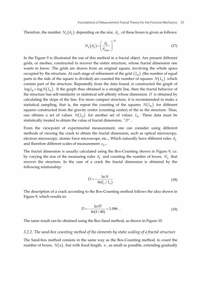
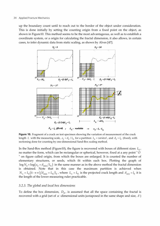
The same result can be obtained using the Box-Sand method, as shown in Figure 10.
3.2.2. The sand-box counting method of the elements by static scaling of a fractal structure
The Sand-box method consists in the same way as the Box-Counting method, to count the number of boxes, N u , but with fixed length, u , as small as possible, extending gradually
Applied Fracture Mechanics 34
up the boundary count until to reach out to the border of the object under consideration. This is done initially by setting the counting origin from a fixed point on the object, as shown in Figure10. This method seems to be the most advantageous, as well as to establish a coordinate system, or a origin for calculating the fractal dimension, it also allows, in certain cases, to infer dynamic data from static scaling, as shown by Alves [47].
Figure 10. Fragment of a crack on test specimen showing the variation of measurement of the crack length L with the measuring scale, 0/k k L for a partition kL variável , and 0k l (fixed), with sectioning done for counting by one-dimensional Sand-Box scaling method.
In the Sand-Box method (Figure10), the figure is recovered with boxes of different sizes kL , no matter the form, which can be rectangular or spherical, however, fixed at a any point " O" on figure called origin, from which the boxes are enlarged. It is counted the number of elementary structures, or seeds, which fit within each box. Plotting the graph of
minlog logk k kN L in the same manner as in the above method the fractal dimension is obtained. Note that in this case the maximum partition is achieved when
min 0 0kN L k L l , where 0L L is the projected crack length and 0min l it is the length of the lower measuring ruler practicable.
3.2.3. The global and local box dimensions
To define the box dimension, BD , is assumed that all the space containing the fractal is recovered with a grid (set of -dimensional units juxtaposed in the same shape and size, )
Foundations of Measurement Fractal Theory for the Fracture Mechanics 35
with maximum size, max , which inscribes the fractal object. Defining the relative scale, on the grid size, max , as being given by:
max
� (20)
countting the number of boxes ( )N that have at least one point of the fractal. The box dimension is therefore defined as:
0
ln ( )limlnBND
(21)
At this point, there are two ways to obtain the actual value of the measure, or taking the limit when 0 and allows that the dimension D fits the end value of ( )N , or it is considered a linear correlation in value of ln ( ) lnN , which D is the slope of the line, and this defines the measure independently of the scale.
In the case of numerical estimation, one can not solve the limit indicated in the equation (21). Then, BD is obtained as a slope, ln ( ) lnN when it is small. The value ( )N is obtained by an algorithm known as Box-Counting.
Self-affine fractals requiring different variations in scale length for different directions. Therefore, one can use the Box-Counting method with some care being taken, in the sense that the box dimension BD to be obtained has a crossing region between a local and global measure of the dimensions. From which follows that for each region is used the following relationships:
0
00 0 00 0
lim /BgD
sl
LN L p L L
l
(22)
for a global measurement
0
00 0 00 0
lim /BlD
sl
LN L p L L
l
(23)
where 0sL is the threshold saturation length which the fractal dimension changes its behavior from local to global stage.
For measurement, generally, for any self-affine fractal structure the local fractal dimension is related to the Hurst exponent, H , as follow,
11Bl qD d H (24)
At this point, one observes that for a profile the relationship 2BlD H commonly used, only serves for a local measurements using the box counting method. While for global
Applied Fracture Mechanics 36
measures one can not establish a relationship between BgD and H . For the global fractal dimension, gD d and 1I d the Euclidean dimension where the fractal is embedded one has
1Bgd D d (25)
Some textbooks on the subject show an example of calculation of local and global fractal dimension of self-affine fractals, obtained by a specific algorithm [18, 22, 23, 26, 38,39].
In crossing the limit of fractal dimension local lD to global gD , there is a transition zone called the "crossover", and the results obtained in this region are somewhat ambiguous and difficult to interpret [39]. However, in the global fractal dimension, the structure is not considered a fractal [42 , 43].
3.2.4. The Relationship between box dimension and HausdorffBesicovitch dimensions
The mathematical definition of generalized dimension of Haussdorff-Besicovitch need a method that can measure it properly to the fractal phenomenon under study. Some authors [23, 40, 44, 45] have discussed the possibility of using the Box-Counting method as one of the graphical methods which obtains a box dimension BD , very close to generalized Haussdorff Besicovitch, HBD , i.e. [44]:
B HBD D (26)
In this sense the box dimension, BD is obtained for self-asimilar fractals that may be rescaled for the same variation in scales lengths in all directions by using the relationship:
00
0
BDL
N Ll
(27)
where 0l is the grid size used and 0L is the apparent size of the fractal to be characterized.
The analytical calculation of the Hausdorff dimension is only possible in some cases and it is difficult to implement by computation. In numerical calculation, is used another more appropriate definition, called box dimension, BD , which in the case of dynamic systems, has the same value of the Haussdorff dimension, D [44]. Thus, it is common to call them without distinction as fractal dimensions, D as will be shown below.
All the definitions related to fractal exponents that are shown here, and all numerical evaluation of these, always calculates the inclination of some amount against on a logarithmic scale.
The two definitions of, Hausdorff-Besicovitch Dimension, HD and Box-Dimension, BD are allocated the same amount, but in a way somewhat different from each other. In inaccurate way, one can think that the connection between the two is done considering that:
Foundations of Measurement Fractal Theory for the Fracture Mechanics 37
~ ,dDM D N (28)
by analogy with equation (13), i.e. approximating to the geometric extension of the object by the number of boxes (of the same size) necessary to recover it. But, since the definition of the box dimension there is no optimization step, and its value is directly dependent on N (which is not the case with the Hausdorff dimension) in practice one has often the geometric extension is overestimated, particularly for large, i. e. upper limit 1 and thus
BD D . However, for the lower limit, i.e. 0 , the Hausdorff-Besicovitch dimensions,
HD and the box dimension, BD are equal, becoming valid the measure of geometric extension process, DM at box counting algorithm.
Considering from (28) that:
~ 1DN d D d , (29)
and that
max max~ 1DN d D d (30)
Therefore, dividing (29) by (30) has:
maxmax
~ 1DN
d D dN
(31)
taking max the total grid extension that recover the object, one has:
max 1 (32)
From as early as (31)
1DN d D d (33)
Substituting (33) in (28) has:
~ ,DDM D (34)
This equation is analogous to the fundamental Richardson relationship for a fractal length.
4. Crack and rugged fracture surface models
The two main problematics of mathematical description of Fracture Mechanics are based on the following aspects: the surface roughness generated in the process and the field stress/strain applied to the specimen. This section deals with the fractal mathematical description of the first aspect, i.e., the roughness of cracks on Fracture Mechanics, using fractal geometry to model its irregular profile. In it will be shown basic mathematical
Applied Fracture Mechanics 38
assumptions to model and describe the geometric structures of irregular cracks and generic fracture surfaces using the fractal geometry. Subsequently, one presents also the proposal for a self-affine fractal model for rugged surfaces of fracture. The model was derived from a generalization of Voss [48] (1) equation and the model of Morel [49] for fractal self-affine fracture surfaces. A general analytical expression for a rugged crack length as a function of the projected length and fractal dimension is obtained. It is also derived the expression of roughness, which can be directly inserted in the analytical context of Classical Fracture Mechanics.
The objectives of this section are: (i) based geometrical concepts, extracted from the fractal theory and apply them to the CFM in order to (ii) construct a precise language for its mathematical description of the CFM, into the new vision the fractal theory. (iii) eliminate some of the questions that arise when using the fractal scaling in the formulation of physical quantities that depend on the rough area of fracture, instead of the projected area, in the manner which is commonly used in fracture mechanics. (iv) another objective is to study the way which the fractal concept can enrich and clarify various aspects of fracture mechanics. For this will be done initially in this section, a brief review of the major advances obtained by the fractal theory, in the understanding of the fractography and in the formation of fracture surfaces and their properties. Then it will be done, also, a mathematical description of our approach, aiming to unify and clarify aspects still disconnected from the classical theory and modern vision, provided by fractal geometry. This will make it possible for the reader to understand what were the major conceptual changes introduced in this work, as well as the point from which the models proposed progressed unfolding in new concepts, new equations and new interpretations of the phenomenon.
4.1. Application of fractal theory in the characterization of a fracture surface
In this section one intends to do a brief history of the fractography development as a fractal characterization methodology of a fractal fracture surface.
4.1.1. Geometric aspects and observations extracted from the quantitative fractography of irregular fracture surface
The technique used for geometric analysis of the fracture surface is called fractography. Until recently it was based only on profilometric study and statistical analysis of irregular surfaces [50]. Over the years, after repeated observations of these surfaces at various magnifications, was also revealed a variety of self-similar structures that lie between the micro and macro-structural level, characteristic of the type of fracture under observation. Since 1950 it is known that certain structures observed in fracture surfaces by microscopy, showed the phenomenon of invariance by magnification. Such structures recently started to be described in a systematic way by means of fractal geometry [51, 25]. This new approach allows the description of patterns that at first sight seem irregular, but keep an invariance by 1 Voss present a fractal description for the noise in the Browniano mouvement
Foundations of Measurement Fractal Theory for the Fracture Mechanics 39
scale transformation (self-similarity or self-affinity). This means that some facts concerning the fracture have the same character independently of the magnification scale, i.e. the phenomenology that give rise to these structures is the same in different observation scales.
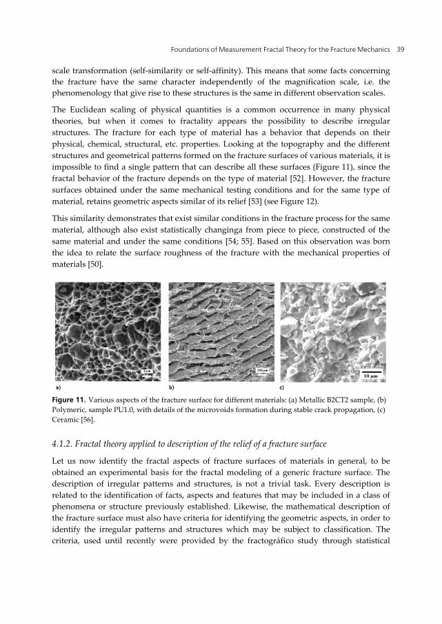
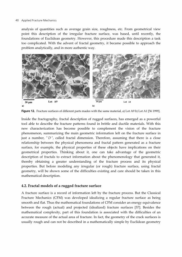
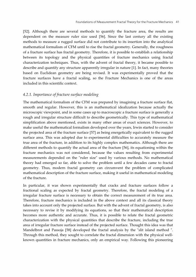
The Euclidean scaling of physical quantities is a common occurrence in many physical theories, but when it comes to fractality appears the possibility to describe irregular structures. The fracture for each type of material has a behavior that depends on their physical, chemical, structural, etc. properties. Looking at the topography and the different structures and geometrical patterns formed on the fracture surfaces of various materials, it is impossible to find a single pattern that can describe all these surfaces (Figure 11), since the fractal behavior of the fracture depends on the type of material [52]. However, the fracture surfaces obtained under the same mechanical testing conditions and for the same type of material, retains geometric aspects similar of its relief [53] (see Figure 12).
This similarity demonstrates that exist similar conditions in the fracture process for the same material, although also exist statistically changinga from piece to piece, constructed of the same material and under the same conditions [54; 55]. Based on this observation was born the idea to relate the surface roughness of the fracture with the mechanical properties of materials [50].
Figure 11. Various aspects of the fracture surface for different materials: (a) Metallic B2CT2 sample, (b) Polymeric, sample PU1.0, with details of the microvoids formation during stable crack propagation, (c) Ceramic [56].
4.1.2. Fractal theory applied to description of the relief of a fracture surface
Let us now identify the fractal aspects of fracture surfaces of materials in general, to be obtained an experimental basis for the fractal modeling of a generic fracture surface. The description of irregular patterns and structures, is not a trivial task. Every description is related to the identification of facts, aspects and features that may be included in a class of phenomena or structure previously established. Likewise, the mathematical description of the fracture surface must also have criteria for identifying the geometric aspects, in order to identify the irregular patterns and structures which may be subject to classification. The criteria, used until recently were provided by the fractográfico study through statistical
Applied Fracture Mechanics 40
analysis of quantities such as average grain size, roughness, etc. From geometrical view point this description of the irregular fracture surface, was based, until recently, the foundations of Euclidean geometry. However, this procedure made this description a task too complicated. With the advent of fractal geometry, it became possible to approach the problem analytically, and in more authentic way.
Figure 12. Fracture surfaces of different parts mades with the same material, a) Lot A9 b) Lot A1 [56 1999].
Inside the fractography, fractal description of rugged surfaces, has emerged as a powerful tool able to describe the fracture patterns found in brittle and ductile materials. With this new characterization has become possible to complement the vision of the fracture phenomenon, summarizing the main geometric information left on the fracture surface in just a number, " D ", called fractal dimension. Therefore, assuming that there is a close relationship between the physical phenomena and fractal pattern generated as a fracture surface, for example, the physical properties of these objects have implications on their geometrical properties. Thinking about it, one can take advantage of the geometric description of fractals to extract information about the phenomenology that generated it, thereby obtaining a greater understanding of the fracture process and its physical properties. But before modeling any irregular (or rough) fracture surface, using fractal geometry, will be shown some of the difficulties existing and care should be taken in this mathematical description.
4.2. Fractal models of a rugged fracture surface
A fracture surface is a record of information left by the fracture process. But the Classical Fracture Mechanics (CFM) was developed idealizing a regular fracture surface as being smooth and flat. Thus the mathematical foundations of CFM consider an energy equivalence between the rough (actual) and projected (idealized) fracture surfaces [57]. Besides the mathematical complexity, part of this foundation is associated with the difficulties of an accurate measure of the actual area of fracture. In fact, the geometry of the crack surfaces is usually rough and can not be described in a mathematically simple by Euclidean geometry
Foundations of Measurement Fractal Theory for the Fracture Mechanics 41
[52]. Although there are several methods to quantify the fracture area, the results are dependent on the measure ruler size used [56]. Since the last century all the existing methods to measure a rugged surface did not contribute to its insertion into the analytical mathematical formalism of CFM until to rise the fractal geometry. Generally, the roughness of a fracture surface has fractal geometry. Therefore, it is possible to establish a relationship between its topology and the physical quantities of fracture mechanics using fractal characterization techniques. Thus, with the advent of fractal theory, it became possible to describe and quantify any structure apparently irregular in nature [1]. In fact, many theories based on Euclidean geometry are being revised. It was experimentally proved that the fracture surfaces have a fractal scaling, so the Fracture Mechanics is one of the areas included in this scientific context.
4.2.1. Importance of fracture surface modeling
The mathematical formalism of the CFM was prepared by imagining a fracture surface flat, smooth and regular. However, this is an mathematical idealization because actually the microscopic viewpoint, and in some cases up to macroscopic a fracture surface is generally a rough and irregular structure difficult to describe geometrically. This type of mathematical simplification above mentioned, exists in many other areas of exact sciences. However, to make useful the mathematical formalism developed over the years, Irwin started to consider the projected area of the fracture surface [57] as being energetically equivalent to the rugged surface area. This was adopted due to experimental difficulties to accurately measure the true area of the fracture, in addition to its highly complex mathematics. Although there are different methods to quantify the actual area of the fracture [56], its equationing within the fracture mechanics was not considered, because the values resulting from experimental measurements depended on the "ruler size" used by various methods. No mathematical theory had emerged so far, able to solve the problem until a few decades came to fractal geometry. Thus, modern fractal geometry can circumvent the problem of complicated mathematical description of the fracture surface, making it useful in mathematical modeling of the fracture.
In particular, it was shown experimentally that cracks and fracture surfaces follow a fractional scaling as expected by fractal geometry. Therefore, the fractal modeling of a irregular fracture surface is necessary to obtain the correct measurement of its true area. Therefore, fracture mechanics is included in the above context and all its classical theory takes into account only the projected surface. But with the advent of fractal geometry, is also necessary to revise it by modifying its equations, so that their mathematical description becomes more authentic and accurate. Thus, it is possible to relate the fractal geometric characterization with the physical quantities that describe the fracture, including the true area of irregular fracture surface instead of the projected surface. Thought this idea was that Mandelbrot and Passoja [58] developed the fractal analysis by the "slit island method ". Through this method, they sought to correlate the fractal dimension with the physical well-known quantities in fracture mechanics, only an empirical way. Following this pioneering
Applied Fracture Mechanics 42
work, other authors [3 , 4 , 5 , 6, 7 , 8, 11, 12, 13, 59 ] have made theoretical and geometrical considerations with the goal of trying to relate the geometrical parameters of the fracture surfaces with the magnitudes of fracture mechanics, such as fracture energy, surface energy, fracture toughness, etc.. However, some misconceptions were made regarding the application of fractal geometry in fracture mechanics.
Several authors have suggested different models for the fracture surfaces [60-63]. Everyone knows that when it was possible to model generically a fracture surface, independently of the fractured material, this will allow an analytical description of the phenomena resulting the roughness of these surfaces within the Fracture Mechanics. Thus the Fracture Mechanics will may incorporate fractal aspects of the fracture surfaces explaining more appropriately the material properties in general. In this section one propose a generic model, which results in different cases of fracture surfaces, seeking to portray the variety of geometric features found on these surfaces for different materials. For this a basic mathematical conceptualization is needed which will be described below. For this reason it is done in the following section a brief bibliographic review of the progress made by researchers of the fractal theory and of the Fracture Mechanics in order to obtain a mathematical description of a fracture surface sufficiently complete to be included in the analytical framework of the Mechanics Fracture.
4.2.2. Literature review - models of fractal scaling of fracture surfaces
Mosolov [64] and Borodich [3 ] were first to associate the deformation energy and fracture surface involved in the fracture with the exponents of surface roughness generated during the process of breaking chemical bonds, separation of the surfaces and consequently the energy dissipation . They did this relationship using the stress field. Mosolov and Borodich [64, 3 ] used the fractional dependence of singularity exponents of this field at the crack tip and the fractional dependence of fractal scaling exponents of fracture surfaces, postulating the equivalence between the variations in deformation and surface energy. Bouchaud [62] disagreed with the Mosolov model [64] and proposed another model in terms of fluctuations in heights of the roughness on fracture surfaces in the perpendicular direction to the line of crack growth, obtaining a relationship between the fracture critical parameters such as ICK and relative variation of the height fluctuations of the rugged surface. In this scenario has been conjectured the universality of the roughness exponent of fracture surfaces because this did not depend on the material being studied [63]. This assumption has generated controversy [61] which led scientists to discover anomalies in the scaling exponents between local and global scales in fracture surfaces of brittle materials. Family and Vicsék [39, 65] and Barabasi [66] present models of fractal scaling for rugged surfaces in films formed by ballistic deposition. Based on this dynamic scaling Lopez and Schimittibuhl [67, 68] proposed an analogous model valid for fracture surfaces, where they observed in your experiments anomalies in the fractal scaling, with critical dimensions of transition for the behavior of the roughness of these surfaces in brittle materials. In this sense Lopez [67, 68] borrowed from the model of Family and Vicsék [39, 65] analogies that could be applied to the rough fracture surfaces.
Foundations of Measurement Fractal Theory for the Fracture Mechanics 43
4.2.3. The fractality of a crack or fracture surface
By observing a crack, in general, one notes that it presents similar geometrical aspects that reproduce itself, at least within a limited range of scales. This property called invariance by scale transformation is called also self-similarity, if not privilege any direction, or self-affinity, when it favors some direction over the other. Some authors define it as the property that have certain geometrical objects, in which its parts are similar to the whole in in successive scales transformation. In the case of fracture, this takes place from a range of minimum cutoff scale , min until a maximum cutoff scale, max , contrary to the proposed by Borodich [3], which defines an infinite range of scales to maintain the mathematical definition fractal. In the model proposed in this section, one used the fractal theory as a form closer to reality to describe the fracture surface with respect to Euclidean description. This was done in order to have a much better approximatation to reality of the problem and to use fractal theory as a more authentic approach.
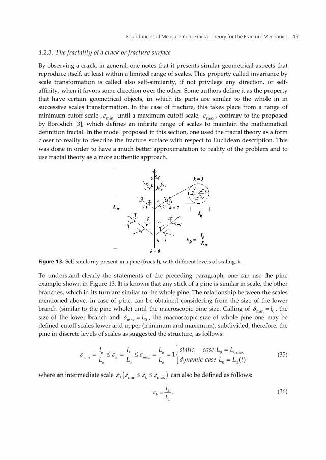
Figure 13. Self-similarity present in a pine (fractal), with different levels of scaling, k.
To understand clearly the statements of the preceding paragraph, one can use the pine example shown in Figure 13. It is known that any stick of a pine is similar in scale, the other branches, which in its turn are similar to the whole pine. The relationship between the scales mentioned above, in case of pine, can be obtained considering from the size of the lower branch (similar to the pine whole) until the macroscopic pine size. Calling of min 0l , the size of the lower branch and max 0L , the macroscopic size of whole pine one may be defined cutoff scales lower and upper (minimum and maximum), subdivided, therefore, the pine in discrete levels of scales as suggested the structure, as follows:
0 0 max
0 0
1( )
o k omin k max
o o o
static case L Ll l Ldynamic case L L tL L L
(35)
where an intermediate scale min maxk k can also be defined as follows:
.kk
o
lL
(36)
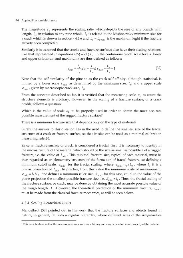
Applied Fracture Mechanics 44
The magnitude k represents the scaling ratio which depicts the size of any branch with length, kl , in relation to any pine whole. 0l is related to the Mishnaevsky minimum size for a crack which is shown in section - 4.2.6 and 0 0 maxL L is the maximum leght if the fracture already been completed.
Similarly it is assumed that the cracks and fracture surfaces also have their scaling relations, like that represented in equations (35) and (36). In the continuous cutoff scale levels, lower and upper (minimum and maximum), are thus defined as follows:
1o omin max
o o o
l LlL L L
(37)
Note that the self-similarity of the pine so as the crack self-affinity, although statistical, is limited by a lower scale min as determined by the minimum size, 0l , and a upper scale
max , given by macroscopic crack size, 0L .
From the concepts described so far, it is verified that the measuring scale k to count the structure elements is arbitrary. However, in the scaling of a fracture surface, or a crack profile, follows a question:
Which is the value of scale k to be properly used in order to obtain the most accurate possible measurement of the rugged fracture surface?
There is a minimum fracture size that depends only on the type of material?
Surely the answer to this question lies in the need to define the smallest size of the fractal structure of a crack or fracture surface, so that its size can be used as a minimal calibration measuring ruler(2).
Since an fracture surface or crack, is considered a fractal, first, it is necessary to identify in the microstructure of the material which should be the size as small as possible a of a rugged fracture, i.e. the value of minl . This minimal fracture size, typical of each material, must be then regarded as an elementary structure of the formation of fractal fracture, so defining a minimum cutoff scale, min , for the fractal scaling, where min 0 0l L , where 0l it is a planar projection of minl . In practice, from this value the minimum scale of measurement,
min 0 0l L one defines a minimum ruler size min , for this case, equal to the value of the plane projection the smallest possible fracture size, i.e. min 0l . Thus, the fractal scaling of the fracture surface, or crack, may be done by obtaining the most accurate possible value of the rough length, L . However, the theoretical prediction of the minimum fracture, minl , must be made from the classical fracture mechanics, as will be seen below.
4.2.4. Scaling hierarchical limits
Mandelbrot [58] pointed out in his work that the fracture surfaces and objects found in nature, in general, fall into a regular hierarchy, where different sizes of the irregularities 2 This must be done so that the measurement scales are not arbitrary and may depend on some property of the material.
Foundations of Measurement Fractal Theory for the Fracture Mechanics 45
described by fractal geometry, are limited by upper and lower sizes, in which each level is a version in scale of the levels contained below and above of these sizes. Some structures that appear in nature, as opposed to the mathematical fractals, present the property of invariance by scale transformation (self- similarity of self-affinity) only within a limited range of scale transformation ( min max ) . Note in Figure 13 that this minimal cutoff scale min , one can find an elementary part of the object similar to the whole, that in iteration rules is used as a seed to construct the fractal pattern that is repeated at successive scales, and the maximum cutoff scale D one can see the fractal object as a whole.
One must not confuse this mathematical recursive construction way, with the way in which fractals appear in nature really. In physical media, fractals appears normally in situations of local or global instability [24], giving rise to structures that can be called fractals, at least within a narrow range of scaling ( min max ) as is the case of trees such as pine, cauliflower, dendritic structures in solidification of materials, cracks, mountains, clouds, etc. From these examples it is observed that, in nature, the particular characteristics of the seed pattern depends on the particular system. For these structures, it is easy to see that that fractal scaling occurs from the lowest branch of a pine, for a example, which is repeated following the same appearance, until the end size of the same, and vice versa. In the case of a crack, if a portion of this crack, is enlarged by a scale, , one will see that it resembles the entire crack and so on, until reaching to the maximum expansion limit in a minimum scale,
min , in which one can not enlarge the portion of the crack, without losing the property of invariance by scaling transformation (self-similar or self-affinity). As the fractal growth theory deals with growing structures, due to local or global instability situations [24], such scaling interval is related to the total energy expended to form the structure. The minimum and maximum scales limit is related to the minimum and maximum scale energy expended in forming the structure, since it is proportional to the fractal mass. The number of levels scaling, k , between min and max depends on the rate at which the formation energy of fractal was dissipated, or also on the instability degree that gave rise to the fractal pattern.
4.2.5. The fractal geometric pattern of a fracture and its measurement scales
Considering that the fracture surface formed follows a fractal behavior necessarily also admits the existence of a geometric pattern that repeats itself, independent of the scale of observation. The existence of this pattern also shows that a certain degree of geometric information is stored in scale, during the crack growth. Thus, for each type of material can be abstract a kind of geometric pattern, apparently irregular with slight statistical variations, able to describe the fracture surface.
Moreover, for the same type of material is necessary to observe carefully the enlargement or reduction scales of the fracture surface. For, as it reduces or enlarges the scale of view, are found pattern and structures which are modified from certain ranges of these scales. This can be seen in Figure 14. In this figure is shown that in an alumina ceramic, whose ampliation of one of its grains at the microstructure reveals an underlying structure of the
Applied Fracture Mechanics 46
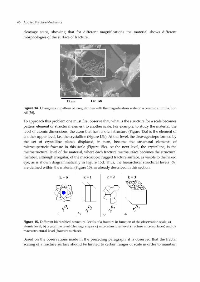
cleavage steps, showing that for different magnifications the material shows different morphologies of the surface of fracture.
Figure 14. Changings in pattern of irregularities with the magnification scale on a ceramic alumina, Lot A8 [56].
To approach this problem one must first observe that, what is the structure for a scale becomes pattern element or structural element to another scale. For example, to study the material, the level of atomic dimensions, the atom that has its own structure (Figure 15a) is the element of another upper level, i.e., the crystalline (Figure 15b). At this level, the cleavage steps formed by the set of crystalline planes displaced, in turn, become the structural elements of microsuperfície fracture in this scale (Figure 15c). At the next level, the crystalline, is the microstructural level of the material, where each fracture microsurface becomes the structural member, although irregular, of the macroscopic rugged fracture surface, as visible to the naked eye, as is shown diagrammatically in Figure 15d. Thus, the hierarchical structural levels [69] are defined within the material (Figure 15), as already described in this section.
Figure 15. Different hierarchical structural levels of a fracture in function of the observation scale; a) atomic level; b) crystalline level (cleavage steps); c) microstructural level (fracture microsurfaces) and d) macrostructural level (fracture surface).
Based on the observations made in the preceding paragraph, it is observed that the fractal scaling of a fracture surface should be limited to certain ranges of scale in order to maintain
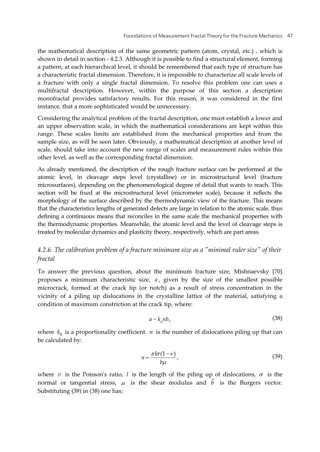
Foundations of Measurement Fractal Theory for the Fracture Mechanics 47
the mathematical description of the same geometric pattern (atom, crystal, etc.) , which is shown in detail in section - 4.2.3. Although it is possible to find a structural element, forming a pattern, at each hierarchical level, it should be remembered that each type of structure has a characteristic fractal dimension. Therefore, it is impossible to characterize all scale levels of a fracture with only a single fractal dimension. To resolve this problem one can uses a multifractal description. However, within the purpose of this section a description monofractal provides satisfactory results. For this reason, it was considered in the first instance, that a more sophisticated would be unnecessary.
Considering the analytical problem of the fractal description, one must establish a lower and an upper observation scale, in which the mathematical considerations are kept within this range. These scales limits are established from the mechanical properties and from the sample size, as will be seen later. Obviously, a mathematical description at another level of scale, should take into account the new range of scales and measurement rules within this other level, as well as the corresponding fractal dimension.
As already mentioned, the description of the rough fracture surface can be performed at the atomic level, in cleavage steps level (crystalline) or in microstructural level (fracture microsurfaces), depending on the phenomenological degree of detail that wants to reach. This section will be fixed at the microstructural level (micrometer scale), because it reflects the morphology of the surface described by the thermodynamic view of the fracture. This means that the characteristics lengths of generated defects are large in relation to the atomic scale, thus defining a continuous means that reconciles in the same scale the mechanical properties with the thermodynamic properties. Meanwhile, the atomic level and the level of cleavage steps is treated by molecular dynamics and plasticity theory, respectively, which are part areas.
4.2.6. The calibration problem of a fracture minimum size as a "minimal ruler size" of their fractal
To answer the previous question, about the minimum fracture size, Mishnaevsky [70] proposes a minimum characteristic size, a , given by the size of the smallest possible microcrack, formed at the crack tip (or notch) as a result of stress concentration in the vicinity of a piling up dislocations in the crystalline lattice of the material, satisfying a condition of maximum constriction at the crack tip, where:
~ ,oa k nb (38)
where 0k is a proportionality coefficient. n is the number of dislocations piling up that can be calculated by:
(1 ) ,lnb
(39)
where v is the Poisson's ratio, l is the length of the piling up of dislocations, is the normal or tangential stress, is the shear modulus and b
is the Burgers vector.
Substituting (39) in (38) one has;

Applied Fracture Mechanics 48
(1 )
~ .ok n la
(40)
Mishnaevsky equates with mathematical elegance, the crack propagation as the result of a "physical reaction" of interaction of a crack size, 0L with a piling up of dislocations, nb , forming a microtrinca size, a , i.e.;
,o oL nb L a (41)
where oa L e onb L .
Mishnaevsky proposes a fractal scaling for the fracture process since the minimum scale, given by the size a , until the maximum scale, given by the macroscopic size crack, 0L .
As a consequence for the existence of a minimum fracture size, recently has arosen a hypothesis that the fracture process is discrete or quantized (Passoja, 1988, Taylor et al., 2005; Wnuk, 2007). Taylor et al. (2005) conducted mathematical changes in CFM to validate this hypothesis. Experimental results have confirmed that a minimum fractures length is given by:
00
2~ .cKl
(42)
where cK is the fracture toughness, 0 is the stress of the yielding strength before the material fracture.
4.2.7. Fractal scaling of a self-similar rough fracture surface or profile
A mathematical relationship between the extension of the self-similar contour and a extension of its projection is calculated as follows.
Being A the surface extension of the fractal contour, given by a self-similar homogenous function with fractional degree, D , where:
.DuA A (43)
0A is the plane projection extension, given by a self-similar homogeneous function with integer degree, d , in accordance with the expression:
0d
uA A , (44)
where, duA is the unit area of measurement, whose values on the rugged and plane
surface are the same. Thus the relationships (43) and (44) can be written in the same way as the equations (43) and (44). Therefore, by dividing these equations, one has:
0 .d DA A (45)
Foundations of Measurement Fractal Theory for the Fracture Mechanics 49
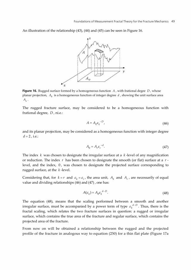
An illustration of the relationship (43), (44) and (45) can be seen in Figure 16.
Figure 16. Rugged surface formed by a homogeneous function A , with frational degee D , whose planar projection, 0A is a homogeneous function of integer degree d , showing the unit surface area
uA .
The rugged fracture surface, may be considered to be a homogeneous function with frational degree, D , ni.e.:
,Dk kA A (46)
and its planar projection, may be considered as a homogeneous function with integer degree 2d , i.e.:
0 .dr rA A (47)
The index k was chosen to designate the irregular surface at a k -level of any magnification or reduction. The index r has been chosen to designate the smooth (or flat) surface at a r -level, and the index, 0 , was chosen to designate the projected surface corresponding to rugged surface, at the k -level.
Considering that, for k r and k r , the area unit, kA and rA , are necessarily of equal value and dividing relationships (46) and (47) , one has:
0( ) .d Dk kA A (48)
The equation (48), means that the scaling performed between a smooth and another irregular surface, must be accompanied by a power term of type d D
k . Thus, there is the
fractal scaling, which relates the two fracture surfaces in question: a rugged or irregular surface, which contains the true area of the fracture and regular surface, which contains the projected area of the fracture.
From now on will be obtained a relationship between the rugged and the projected profile of the fracture in analogous way to equation (250) for a thin flat plate (Figure 17a
Applied Fracture Mechanics 50
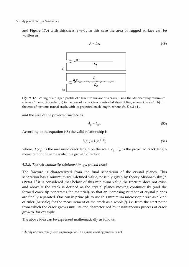
and Figure 17b) with thickness 0e . In this case the area of rugged surface can be written as:
,A Le (49)
Figure 17. Scaling of a rugged profile of a fracture surface or a crack, using the Mishnaevsky minimum size as a "measuring ruler"; a) in the case of a crack is a non-fractal straight line, where 1D d ; b) in the case of tortuous fractal crack, with its projected crack length, where 1d D d .
and the area of the projected surface as
0 0 ,A L e (50)
According to the equation (48) the valid relationship is:
( ) ,d Dk o kL L (51)
where, ( )kL is the measured crack length on the scale k , 0L is the projected crack length measured on the same scale, in a growth direction.
4.2.8. The self-similarity relationship of a fractal crack
The fracture is characterized from the final separation of the crystal planes. This separation has a minimum well-defined value, possibly given by theory Mishnaevsky Jr. (1994). If it is considered that below of this minimum value the fracture does not exist, and above it the crack is defined as the crystal planes moving continuously (and the formed crack tip penetrates the material), so that an increasing number of crystal planes are finally separated. One can in principle to use this minimum microscopic size as a kind of ruler (or scale) for the measurement of the crack as a whole(3), i.e. from the start point from which the crack grows until its end characterized by instantaneous process of crack growth, for example.
The above idea can be expressed mathematically as follows:
3 During or concurrently with its propagation, in a dynamic scaling process, or not
Foundations of Measurement Fractal Theory for the Fracture Mechanics 51
0 ,d DL L (52)
dividing the entire expression (52) above by the minimum Mishnaevsky size one has:
0 ,d DLLa a
(53)
or
0 ,d DN N (54)
where
N L a : is the number of crack elements a on the non-projected crack
0 0N L a : is the number of cracl elements a on the crack projected
and yet:
0 ,a L (55)
where:
: is the scaling factor of the fractal crack
d : is the Euclidean dimension of the crack projection
D : is the crack fractal dimension.
Within this context the number of microcracks that form the macroscopic crack is given by:
.D
o
aNL
(56)
In this context (in Mishnaevsky model), the above expression is volumetric and admits cracks branching generated in the fracture process with opening and coalescence of microcracks. However, he continue equating the process in a one-dimensional way reaching an expression for the crack propagation velocity. A complete discussion of this subject, using a self-affine fractal model to be more realistic and accurate, can be done in another research paper.
The answer to the question about what should be the best scale to be used for fractal fracture scaling is then given as follows: being the limit of the crack length kL in any scale, given by
kL L (actual size) as well as minkl l , the value of the minimum size ruler, 0l it must be equal to the minimum crack size, a (4), given by Mishnaevsky [70], through its energy balance for the fracture of a single monocrystal of the microstructure of a material. The physical reason for this choice is because the Mishnaevsky minimum size is determined by a 4 It is possible that this minimal ruler size be very low than the scale used in fractal characterization of the fracture surfaces. However, it must to be the smallest possible size for a microcrack.
Applied Fracture Mechanics 52
energy balance, from which the crack comes to exist, because below this size, there is no sense speak of crack length. Therefore, the scale that must be considered is given by:
min 0a L , (57)
where a is given by relation (40).
Therefore, the statistical self-similarity or self-affinity of a fracture surface, or a crack is limited by a cutoff lower scale min , determined by the minimum critical size, 0l a , and a cutoff upper scale max , given by the macroscopic crack length, 0L .
In two dimensions, the problem of existence of a minimum scale size (possibly given by the Mishnaevky minimum size), leads to abstraction of a microsurface with minimum area, whose shape will be investigated further, in Appendices, in terms of the number of stress concentrators nearest existing within a material.
4.3. Model of self-affine fracture surface or profiles
In this section one intend to present the development of fractal models of self-similar surfaces. From a rough fracture surface can be extracted numerous profiles also rough on the crack propagation direction. However, in this section is considered only one profile, which is representative of the entire fracture surface (Figure 18). The plane strain condition admits this assumption. Because, although the fracture toughness varies along the thickness of the material to a plastic zone reduced in relation to material thickness, it can be considered a property. This means that it is possible to obtain a statistically rough profile, equivalent to other possible profiles, which can be obtained within the thickness range considered by plane strain conditions.
Figure 18. Statistically equivalent profiles along the thickness of the material
In order also equivalent to this, it is also possible to obtain an average projected crack length as a result of an average of the crack size along the thickness of the material thickness within the range considered by plane strain, for the purpose of calculations in CFM, it is considered
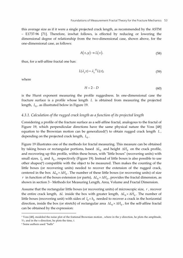
Foundations of Measurement Fractal Theory for the Fracture Mechanics 53
this average size as if it were a single projected crack length, as recommended by the ASTM – E1737-96 [71]. Therefore, inwhat follows, is effected by reducing or lowering the dimensional degree of relationship from the two-dimensional case, shown above, for the one-dimensional case, as follows:
, .A x y L x (58)
thus, for a self-affine fractal one has:
( ) ( ),Hx xL x L x (59)
where
2H D (60)
is the Hurst exponent measuring the profile ruggedness. In one-dimensional case the fracture surface is a profile whose length L is obtained from measuring the projected length, 0L , as illustrated below in Figure 19.
4.3.1. Calculation of the rugged crack length as a function of its projected length
Considering a profile of the fracture surface as a self-affine fractal, analogous to the fractal of Figure 19, which perpendicular directions have the same physical nature the Voss [48] equation to the Brownian motion can be generalized(5) to obtain rugged crack length L , depending on the projected crack length, 0L .
Figure 19 illustrates one of the methods for fractal measuring. This measure can be obtained by taking boxes or rectangular portions, based 0L and height 0H on the crack profile, and recovering up this profile, within these boxes, with "little boxes" (recovering units) with small sizes, 0l and 0h , respectively (Figure 19). Instead of little boxes is also possible to use other shapes(6) compatible with the object to be measured. Then makes the counting of the little boxes (or recovering units) needed to recover the extension of the rugged crack, centered in the box 0 0L H . The number of these little boxes (or recovering units) of size r in function of the boxes extension (or parts), 0 0L H , provides the fractal dimension, as shown in section 3 - Methods for Measuring Length, Area, Volume and Fractal Dimension.
Assume that the rectangular little boxes (or recovering units) of microscopic size, r , recover the entire crack length, L inside the box with greater length, 0 0L H . The number of little boxes (recovering unit) with sides of 0 0l h needed to recover a crack in the horizontal direction, inside the box (or stretch) of rectangular area 0 0L H , for the self-affine fractal can be obtained by the expression: 5 Voss [48], modeled the noise plot of the frational Brownian motion , where in the y-direction, he plots the amplitude, VH, and in the x-direction, he plots the time, t. 6 Some authors used “balls”
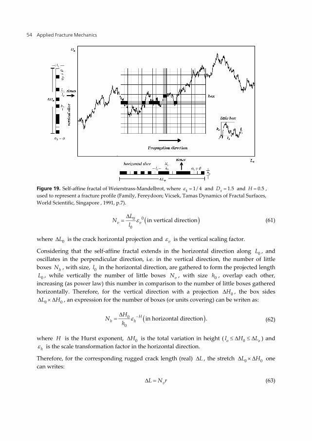
Applied Fracture Mechanics 54
Figure 19. Self-affine fractal of Weierstrass-Mandelbrot, where 1 / 4k and 1.5xD and 0.5H , used to represent a fracture profile (Family, Fereydoon; Vicsek, Tamas Dynamics of Fractal Surfaces, World Scientific, Singapore , 1991, p.7).
00
0in vertical directionv v
LN
l
(61)
where 0L is the crack horizontal projection and v is the vertical scaling factor.
Considering that the self-affine fractal extends in the horizontal direction along 0L , and oscillates in the perpendicular direction, i.e. in the vertical direction, the number of little boxes hN , with size, 0l in the horizontal direction, are gathered to form the projected length
0L , while vertically the number of little boxes vN , with size 0h , overlap each other, increasing (as power law) this number in comparison to the number of little boxes gathered horizontally. Therefore, for the vertical direction with a projection 0H , the box sides
0 0L H , an expression for the number of boxes (or units covering) can be writen as:
0
0in horizontal direction .H
h hH
Nh
(62)
where H is the Hurst exponent, 0H is the total variation in height ( 0o ol H L ) and
h is the scale transformation factor in the horizontal direction.
Therefore, for the corresponding rugged crack length (real) L , the stretch 0 0L H one can writes:
vL N r (63)

Foundations of Measurement Fractal Theory for the Fracture Mechanics 55
where r is equal to the rugged crack length on a microscopic scale, as a function of extension of the little boxes 0 0l h by:
2 20 0r l h (64)
where 0l and 0h are the microscopic sizes of the crack length in horizontal and vertical directions, respectively. Substituting (64) in (63), one has:
2 20 0vL N l h (65)
substituting (61) in (65), one has:
2 200 0
0
LL l h
l
(66)
Since that in the fracture process, the scales in orthogonal directions are the same physical nature, one can choose 0 0/v h l L , and one can writes from (62) that:
0 0
0 0
H
hH L
Nl l
(67)
being necessarily h vN N , one has:
0 0 0
0 0 0
HL H Ll l l
(68)
rewriting the equation (66), one has:
2
00
01
hL L
l
(69)
writing 0h from (68), as:
1
00 0
0.
HL
h Hl
(70)
Eliminating in (69) the dependence of 0h , by substituting (70) in (69), one has:
2 2 1
0 00
0 01
HH L
L Ll l
(71)
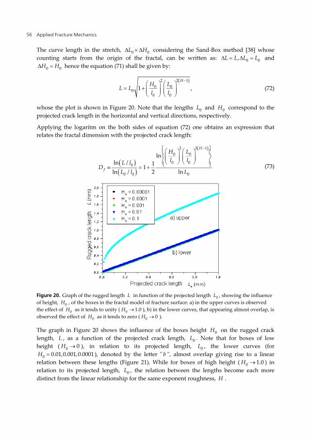
Applied Fracture Mechanics 56
The curve length in the stretch, 0 0L H considering the Sand-Box method [38] whose counting starts from the origin of the fractal, can be written as: 0 0,L L L L and
0 0H H hence the equation (71) shall be given by:
2 2 1
0 00
0 01 ,
HH L
L Ll l
(72)
whose the plot is shown in Figure 20. Note that the lengths 0L and 0H correspond to the projected crack length in the horizontal and vertical directions, respectively.
Applying the logaritm on the both sides of equation (72) one obtains an expression that relates the fractal dimension with the projected crack length:
2 2 10 0
0 00
00 0
lnln / 11
2 lnln /
H
f
H Ll lL l
DLL l
(73)
Figure 20. Graph of the rugged length L in function of the projected length 0L , showing the influence of height, 0H , of the boxes in the fractal model of fracture surface: a) in the upper curves is observed the effect of 0H as it tends to unity ( 0 1.0H ), b) in the lower curves, that appearing almost overlap, is observed the effect of 0H as it tends to zero ( 0 0H ).
The graph in Figure 20 shows the influence of the boxes height 0H on the rugged crack length, L , as a function of the projected crack length, 0L . Note that for boxes of low height ( 0 0H ), in relation to its projected length, 0L , the lower curves (for
0 0.01,0.001,0.0001H ), denoted by the letter " b ", almost overlap giving rise to a linear relation between these lengths (Figure 21). While for boxes of high height ( 0 1.0H ) in relation to its projected length, 0L , the relation between the lengths become each more distinct from the linear relationship for the same exponent roughness, H .
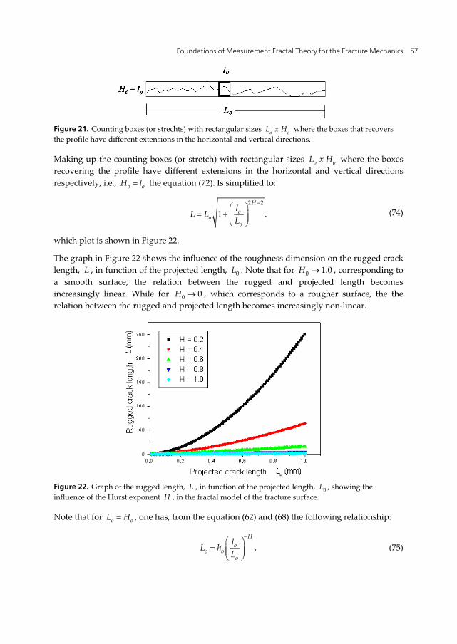
Foundations of Measurement Fractal Theory for the Fracture Mechanics 57
Figure 21. Counting boxes (or strechts) with rectangular sizes o oL x H where the boxes that recovers the profile have different extensions in the horizontal and vertical directions.
Making up the counting boxes (or stretch) with rectangular sizes o oL x H where the boxes recovering the profile have different extensions in the horizontal and vertical directions respectively, i.e., o oH l the equation (72). Is simplified to:
2 2
1 .H
oo
o
lL L
L
(74)
which plot is shown in Figure 22.
The graph in Figure 22 shows the influence of the roughness dimension on the rugged crack length, L , in function of the projected length, 0L . Note that for 0 1.0H , corresponding to a smooth surface, the relation between the rugged and projected length becomes increasingly linear. While for 0 0H , which corresponds to a rougher surface, the the relation between the rugged and projected length becomes increasingly non-linear.
Figure 22. Graph of the rugged length, L , in function of the projected length, 0L , showing the influence of the Hurst exponent H , in the fractal model of the fracture surface.
Note that for o oL H , one has, from the equation (62) and (68) the following relationship:
,H
oo o
o
lL h
L
(75)
Applied Fracture Mechanics 58
which is a self-similar relation between the projected crack length, 0L , and height of the little box, 0h . This relationship shows that all self-affine fractal, in the approximation of a small scale, has a local self-similarity forming a fractal substructure, when is considered square portions, 0 0L L , instead of rectangular portions, 0 0L H .
It important to observe that 0L denotes the distance between two points of the crack (the projected crack length). The self-affine measure, L of 0L , in the fractal dimension, D , is given by (72). 0l is the possible minimum length of a micro-crack, which defines the scale
0 0/l L under which the crack profile is scrutinized, as discussed in previous section and will be discussed after in the section #.5.4.5. The Hurst exponent, H , is related to D by (60).
In the study of a self-affine fractal there are two extremes limits to be verified. One is the limit at which the boxes height is high in relation to its projected length, 0L , i.e. ( 0 0H L ), which is also called local limit. The other limit is one in which the boxes height is low in relation to its projected length, 0L , i.e., ( 0 0H h ) which is called global limit. It will be seen now each one of this limits case contained in the expression (72).
Case 1 : The self-similar or local limit of the fractality
Taking the local limit of the self-affine fractal measure as given by (72), i. e. for the case where, 0 0 0H L l , one has:
1H
oo
o
lL L
L
(76)
where
12
HoH
o
L l constantL
(77)
This equation is analogous to self-similar mathematical relationship only that the exponent is 1 H instead of 1D , which satisfies the relation 2H D [3 , 40, 51 , 70].
According to these results it is observed that the relation (77) has a commitment to the Hurst exponent of the profiles on the considered observation scale 0 0/l L . It is observed that the consideration of a minimum fracture size 01l over a region, one must consider the local dimension of the fracture roughness on this scale. Similarly, if the considerations of a minimum fracture size are made in a scale that involves several regions, 02l this should take into account the value of the roughness global dimension on this scale, so that:
1 21 11 01 2 02(2 ) (2 ) ,H HH l H l constant (78)
although 01 02l l e 1 2H H .
Case 2: The self-affine or global limit of fractality
Taking the global limit of the self-affine fractal measure given by (72), i.e. for the case in which: 0 0 0H l L . Therefore the length L is independently of H and 1D , so
Foundations of Measurement Fractal Theory for the Fracture Mechanics 59
oL L (79)
It must be noted that the ductile materials by having a high fractality have a crack profile which can be better fitted by the equation (76), while brittle materials by having a low fractality will be better fitted by the equation (79) corresponding the classical model, i.e., a flat geometry for the fracture surface. Furthermore, the cleavage which occurs on the microstructure of ductile materials tend to produce a surface, where 0L L , which could be called smooth. However, this cleavage effect is just only local in these materials and therefore the resulting fracture surface is actually rugged.
4.3.2. Local Ruggedness of a fracture surface
Defining the local roughness of a fracture surface, as:
0 0.o
dA A A dAdA
(80)
where A is the rugged surface and 0A is the projected surface. In the case of a rugged crack profile,one has:
0 0o
dL L L dLdL
(81)
using (74) in (81), one has that:
2 2
2 2
1 (2 )
1
Ho
oH
o
o
lH
L
lL
(82)
From (81) note that when there is no roughness on surfaces (flat fracture) one has that:
0L L , thus
1.o
dLdL
(83)
The quantity o
dLdL
seems be a good definition of ruggedness unlike the definition where
the ruggedness is given by / //L L [56, 57] (where / / 0 cosML L , see Figure 23) does not
satisfy the requirement intuitive of the ruggednes when 0ML is only inclined with respect to
0L , while maintaining, 0 0ML L , as shown Figure 23.
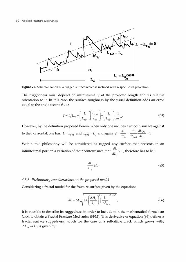
Applied Fracture Mechanics 60
Figure 23. Schematization of a rugged surface which is inclined with respect to its projection.
The ruggedness must depend on infinitesimally of the projected length and its relative orientation to it. In this case, the surface roughness by the usual definition adds an error equal to the angle secant , or
0/ /
0 / / 0
1 .cos
M
M M
LL LL LL L L
(84)
However, by the definition proposed herein, when only one inclines a smooth surface against
to the horizontal, one has: 0ML L and 0 0ML L and again, 1oM
o oM o
dLdL dLdL dL dL
.
Within this philosophy will be considered as rugged any surface that presents in an
infinitesimal portion a variation of their contour such that 1o
dLdL
, therefore has to be:
1o
dLdL
. (85)
4.3.3. Preliminary considerations on the proposed model
Considering a fractal model for the fracture surface given by the equation:
2 2 2
1 ,H
o oo
o o
H lL L
l L
(86)
it is possible to describe its ruggedness in order to include it in the mathematical formalism CFM to obtain a Fractal Fracture Mechanics (FFM). This derivative of equation (86) defines a fractal surface ruggedness, which for the case of a self-affine crack which grows with,
0 0H l , is given by:
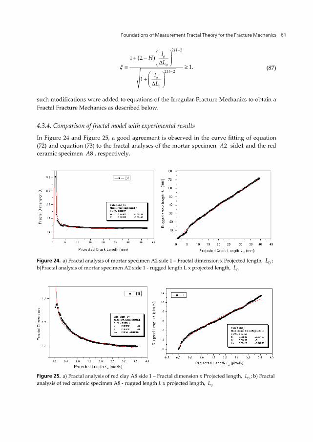
Foundations of Measurement Fractal Theory for the Fracture Mechanics 61
2 2
2 2
1 (2 )1.
1
Ho
oH
o
o
lH
L
lL
(87)
such modifications were added to equations of the Irregular Fracture Mechanics to obtain a Fractal Fracture Mechanics as described below.
4.3.4. Comparison of fractal model with experimental results
In Figure 24 and Figure 25, a good agreement is observed in the curve fitting of equation (72) and equation (73) to the fractal analyses of the mortar specimen 2A side1 and the red ceramic specimen 8A , respectively.
Figure 24. a) Fractal analysis of mortar specimen A2 side 1 – Fractal dimension x Projected length, 0L ; b)Fractal analysis of mortar specimen A2 side 1 - rugged length L x projected length, 0L
Figure 25. a) Fractal analysis of red clay A8 side 1 – Fractal dimension x Projected length, 0L ; b) Fractal analysis of red ceramic specimen A8 - rugged length L x projected length, 0L
Applied Fracture Mechanics 62
5. Conclusions
i. It is possible, in principle, mathematically distinguish a crack in different materials using geometric characteristics which can be portrayed by different values of roughness exponents in the relations (72) and (74).
ii. The fractal model of the rugged crack length, L in function of the projected crack length, 0L , suggested by Alves [72 73 ,74 , 75 ] seems have a good agreement with experimental results. This results allowed us to consolidate the model previously published in the literature on fracture [72 , 73 , 75 ].
iii. The rugged crack length is a response to its interaction with the microstructure. of the material. Therefore, mathematically is possible to portray the rugged peculiar behavior of a crack using fractal geometry
iv. The mathematical model presents a wealth (mathematical richness) that can still be explored in terms of determining the minimum crack length, 0l for each material and the fractal dimension as a function of test parameters and material properties.
v. The mathematical model is sensitive to variations in the behavior of the crack length it is a linear or logarithmic with the projected crack length.
Comparing the experimental results with the model proposed in this chapter, it is concluded that one of the more important results obtained here are the equations (72), (74) and (82) leading to finding that the fracture surfaces of the materials analyzed are indeed (actually) self-affine fractals. Starting from this verification it becomes feasible to consider the fractal model of rugged fracture surface and its ruggedess inside the equations of the classical fracture mechanics, according to equation (74) and (82). As there is a close relationship between phenomenology and structure formed by virtue of its fractal geometry, the understanding of the formation processes of these dissipative structures, as the cracks, should be derived from their mathematical analysis, as the close relationship between the phenomenology of the formation process of dissipative structures and their fractal geometry. Therefore, the mathematical description of fractal structures must exceed a simple geometrical characterization, in order to correlate the pattern formed in the process of energy dissipation with the amount of energy dissipated in the process that generated it. Thus, it is possible to use the fractal geometry in order to understand other more and more complex processes inside the fracture mechanics. Therefore, the various mechanisms responsible by the crack deviation and by the formation of the rugged fracture surface can then, from the fractal model, be quantified in the fractal analysis of this surface.
The idea of obtaining a relationship between L and 0L comes the need to maintain the present formalism used by the CFM, showing that fractal geometry can greatly contribute to the continued advancement of this science.
On the other hand, we are interested in developing a Fractal Thermodynamic for a rugged crack that will be related to the CFM and the Classical Fracture Thermodynamics when the crack ruggedness is neglected or the crack is considered smooth.
Foundations of Measurement Fractal Theory for the Fracture Mechanics 63
Author details
Lucas Máximo Alves GTEME – Grupo de Termodinâmica, Mecânica e Eletrônica dos Materiais, Departamento de Engenharia de Materiais, Setor de Ciências Agrárias e de Tecnologia, Universidade Estadual de Ponta Grossa, Brazil
6. References [1] Mandelbrot, Benoit B. (1982) The Fractal Geometry of Nature. San Francisco, Cal-Usa,
New York: W. H. Freeman and Company. 472 p. [2] Rodrigues, J. A. E V. C. Pandolfelli (1996) Dimensão Fractal E Energia Total de Fratura.
Cerâmica, Maio/Junho. 42(275). [3] Borodich, F. M. (1997) Some Fractals Models of Fracture. J. Mech. Phys. Solids. 45(2):239-259. [4] Heping, Xie (1989) The Fractal Effect of Irregularity of Crack Branching on the Fracture
Toughness of Brittle Materials. International Journal of Fracture. 41: 267-274. [5] Mu, Z. Q. and C. W. Lung (1988) Studies on the Fractal Dimension and Fracture
Toughness of Steel. J. Phys. D: Appl. Phys. 21: 848-850. [6] Mecholsky, J. J.; D. E. Passoja and K. S. Feinberg-Ringel (1989) Quantitative Analysis of
Brittle Fracture Surfaces Using Fractal Geometry. J. Am. Ceram. Soc. 72( 1): 60-65. [7] Lin, G. M.; J. K. L. Lai (1993) Fractal Characterization of Fracture Surfaces In a Resin-
Based Composite. Journal of Materials Science Letters. 12: 470-472. [8] Nagahama, Hiroyuki (1994) A Fractal Criterion for Ductile and Brittle Fracture. J. Appl.
Phys. 15 March, 75(6): 3220-3222. [9] Lei, Weisheng and Bingsen Chen (1994) Discussion on “The Fractal Effect of Irregularity
of Crack Branching on the Fracture Toughness of Brittle Materials” By Xie Heping. International Journal of Fracture. 65: R65-R70.
[10] Lei, Weisheng and Bingsen Chen (1994) Discussion: “Correlation Between Crack Tortuosity and Fracture Toughness In Cementitious Material” By M. A. Issa, A. M. Hammad and A. Chudnovsky, A. International Journal of Fracture. 65: R29-R35.
[11] Lei, Weisheng and Bingsen Chen (1995) Fractal Characterization of Some Fracture Phenomena, Engineering Fracture Mechanics. 50(2): 149-155.
[12] Tanaka, M. (1996) Fracture Toughness and Crack Morphology In Indentation Fracture of Brittle Materials. Journal of Materials Science. 31: 749-755.
[13] Chelidze, T.; Y. Gueguen ( 1990) Evidence of Fractal Fracture, (Technical Note) Int. J. Rock. Mech Min. Sci & Geomech Abstr. 27( 3): 223-225.
[14] Herrmann, H. J.; Kertész, J.; de Arcangelis, L. (1989) Fractal Shapes of Deterministic Cracks. Europhys. Lett. 10(2): 147-152.
[15] De Arcangelis, L.; Hansen A; Herrmann, H. J. (1989) Scaling Laws In Fracture. Phys. Review B. 1 July 40(1).
[16] Herrmann, Hans J. (1986) Growth: An Introduction. In: H. Eugene Stanley and Nicole Ostrowskym editors. On the Growth and Form, Fractal and Non-Fractal Patterns In Physics, Nato Asi Series, Series E: Applied Sciences N. 100 (1986), Proc. of the Nato Advanced Study Institute Ön Growth and Form”, Cargese, Corsiva, France June 27-July 6 1985. Copyright By Martinus Nighoff Publishers, Dordrecht.
[17] Tsallis, C.; Plastino, A. R.; and Zheng, W.-M. (1997) Chaos, Solitons & Fractals 8: 885.
Applied Fracture Mechanics 64
[18] Mccauley, Joseph L. (1993) Chaos, Dynamics and Fractals: An Algorithmic Approach To Deterministic Chaos, Cambridge Nonlinear Science Series, Vol. 2, Cambridge England: Cambridge University Press.
[19] Stanley, H. Eugene (1973) Introduction To Phase Transitions and Critical Phenomena. (Editors: Cooperative Phenomena Near Phase Transitions, a Bilbiography With Selected Readings, Mit,). Cambridge, Massachusetts : Claredon Oxford
[20] Uzunov, D. I. (1993) Theory of Critical Phenomena, Mean Field, Flutuactions and Renormalization. Singaore: World Scientific Publishing Co. Pte. Ltd.
[21] Beck, C. and F. Schlögl (1993) Thermodynamics of Chaotic Systems: An Introduction, Cambridge Nonlinear Science Series, Vol. 4, Cambridge England: Cambridge University Press,.
[22] Meakin, Paul (1995) Fractal Growth: , Cambridge Nonlinear Science Series, Vol. 5, England: Cambridge University Press.
[23] Vicsék, Tamás (1992) Fractal Growth Phenonmena. Singapore: World Scientific. [24] Sander, L. M. (1984) Theory of Fractal Growth Process In: F. Family, D. P. Landau
editors. Kinetics of Aggregation and Gelation. Amsterdam: Elsevier Science Publishers B. V. pp. 13-17.
[25] Meakin, Paul (1993) The Growth of Rough Surfaces and Interfaces. Physics Reports. December 235(485): 189-289.
[26] Pietronero, L.; Erzan, A.; Everstsz, C. (1988) Theory of Fractal Growth. Phys. Revol. Lett. 15 August 61(7): 861-864.
[27] Herrmann, Hans J.; Roux, Stéphane (1990) Statistical Models For the Fracture of Disordered Media, Random Materials and Processes Series. H. Eugene Stanley and Etienne Guyon editors., Amsterdam: North-Holland.
[28] Charmet, J. C. ; Roux , S and Guyon, E. (1990) Disorder and Fracture. New York: Plenum Press. [29] Meakin, Paul; Li, G.; Sander, L. M.; Louis, E.; Guinea, F. (1989) A Simple Two-
Dimensional Model For Crack Propagation. J. Phys. A: Math. Gen. 22: 1393-1403. [30] Gross, Steven. P.; Jay. Fineberg, M. P. Marder, W. D. Mccormick and Harry. L. Swinney
(1993) Acoustic Emissions From Rapidly Moving Cracks. Physical Review Letters. , 8 November 71(19): 3162-3165.
[31] Sharon, Eran; Steven Paul Gross and Jay Fineberg (1996) Energy Dissipation In Dynamic Fracture. Physical Review Letters. 18 March, 76(12): 2117-2120.
[32] Hausdorff F. (1919) Dimension Und Äußeres Maß. Mathematische Annalen March 79(1–2): 157–179. Doi:10.1007/Bf01457179.
[33] Besicovitch, A. S. (1929) On Linear Sets of Points of Fractional Dimensions. Mathematische Annalen 101.
[34] Besicovitch, A. S. H. D. Ursell. (1937) Sets of Fractional Dimensions. Journal of the London Mathematical Society 12, 1937. Several Selections From This Volume Are Reprinted In Edgar, Gerald A. (1993). Classics on Fractals. Boston: Addison-Wesley. Isbn 0-201-58701-7. See Chapters 9,10,11
[35] Mandelbrot, Benoit B (1975) Fractal.. [36] Mandelbrot, Benoit B (1977) Fractals: Form Chance and Dimension. San Francisco, Cal-
USA: W. H. Freeman and Company. [37] Alves, Lucas Máximo (2012) Application of a Generalized Fractal Model For Rugged
Fracture Surface To Profiles of Brittle Materials. Paper in preparation.
Foundations of Measurement Fractal Theory for the Fracture Mechanics 65
[38] Bunde, Armin Shlomo Havlin (1994) Fractals In Science. Springer-Verlag. [39] Family, Fereydoon; Vicsek, Tamás (1991) Dynamics of Fractal Surfaces. Singapore:
World Scientific Publishing Co. Pte. Ltd. P.7-8, P. 73-77. [40] Feder, Jens (1989) Fractals, New York: Plenum Press. [41] Barnsley, Michael (1988) Fractals Everywhere, Academic Press, Inc, Harcourt Brace
Jovanovich Publishers. [42] Milman V. Yu., Blumenfeld R., Stelmashenko N. A. and Ball R. C. (1993) Phys. Rev. Lett.
71 , 204. [43] Milman, Victor Y.; Nadia A. Stelmashenko and Raphael Blumenfeld (1994) Fracture
Surfaces: a Critical Review of Fractal Studies and a Novel Morphological Analysis of Scanning Tunneling Microscopy Measurements, Progreess In Materials Science. 38: 425-474.
[44] Yamaguti, Marcos (1992). Doctoral Thesis - Universidade de São Paulo [45] Allen, Martin; Gareth J. Brown; Nick J. Miles (1995) Measurements of Boundary Fractal
Dimensions: Review of Current Techniques. Powder Technology. 84:1-14. [46] Richardson, L. F. (19161) The Problem of Contiguity: An Appendix To Statistics of
Deadly Quarrels. General Systems Yearbook. (6): 139-187. [47] Alves, Lucas Máximo (1998) Escalonamento Dinâmico da Fractais Laplacianos Baseado
No Método Sand-Box, In: Anais Do 42o Cong. Bras. de Cerâmica, Poços de Caldas de 3 a 6 de Junho,. Artigo Publicado neste Congresso Ref.007/1.
[48] Voss, Richard F. (1991) In: Family, Fereydoon. and Vicsék, Tamás, editors. Dynamics of Fractal Surfaces. Singapore: World Scientific. pp. 40-45.
[49] Morel, Sthéphane, Jean Schmittbuhl, Elisabeth Bouchaud and Gérard Valentin (2000) Scaling of Crack Surfaces and Implications on Fracture Mechanics Arxiv:Cond-Mat/0007100 6 Jul 2000, vol. 1, Or Phys. Rev. Lett. 21 August 85(8).
[50] Underwood, Erwin E. and Kingshuk Banerji (1996) Quantitative Fractography. Engineering Aspectes of Failure and Failure Analysis - Asm - Handbook - Vol. 12, Fractography - the Materials Information Society (1992). Astm 1996 , pp. 192-209
[51] Dauskardt, R. H.; F. Haubensak and R. O. Ritchie (1990) On the Interpretation of the Fractal Character of Fracture Surfaces; Acta Metall. Matter. 38(2): 143-159.
[52] Underwood, Erwin E. and Kingshuk Banerji (1986) Fractals In Fractography, Materials Science and Engineering, Ed. Elsevier. 80: pp. 1-14.
[53] Underwood, Erwin E. and Kingshuk Banerji (1996) Fractal Analysis of Fracture Surfaces. Engineering Aspectes of Failure and Failure Analysis - Asm - Handbook - Vol. 12, Fractography - the Materials Information Society (1992), Astm 1996. pp. 210-215
[54] Alves, L. M. ; Chinelatto, Adilson Luiz ; Chinelatto, Adriana Scoton Antonio ; Prestes, Eduardo (2004) Verificação de um modelo fractal de fratura de argamassa de cimento. In: Anais do 48º Congresso Brasileiro de Cerâmica, 28 de Junho a 1º de Julho de 2004, Em Curitiba – Paraná.
[55] Alves, L. M. ; Chinelatto, Adilson Luiz ; Chinelatto, Adriana Scoton Antonio ; Grzebielucka, Edson Cezar (2004) Estudo do perfil fractal de fratura de cerâmica vermelha. In: Anais do 48º Congresso Brasileiro de Cerâmica, 28 de Junho a 1º de Julho de 2004, Em Curitiba – Paraná.
[56] Dos Santos, Sergio Francisco (1999) Aplicação Do Conceito de Fractais Para Análise Do Processo de Fratura de Materiais Cerâmicos, Master Dissertation, Universidade Federal
Applied Fracture Mechanics 66
de São Carlos. Centro de Ciências Exatas e de Tecnologia, Programa de Pós-Graduação em Ciência e Engenharia de Materiais, São Carlos.
[57] Anderson, T. L. (1995) Fracture Mechanics, Fundamentals and Applications. Crc Press, 2th Edition.
[58] Mandelbrot, Benoit B.; Dann E. Passoja & Alvin J. Paullay (1984) Fractal Character of Fracture Surfaces of Metals, Nature (London). 19 April, 308 [5961]: 721-722.
[59] Lung, C. W. and Z. Q. Mu, (1988)n Fractal Dimension Measured With Perimeter Area Relation and Toughness of Materials, Physical Review B. 1 December , 38( 16): 11781-11784.
[60] Bouchaud, Elisabeth (1977) Scaling Properties of Crack. J. Phys: Condens. Matter. 9: 4319-4344.
[61] Bouchaud, E.; G. Lapasset and J. Planés (1990) Fractal Dimension of Fractured Surfaces: a Universal Value? Europhysics Letters. 13(1): 73-79.
[62] Bouchaud, E.; J. P. Bouchaud (1994-I) Fracture Surfaces: Apparent Roughness, Relevant Length Scales, and Fracture Toughness. Physical Review B. 15 December . 50(23): 17752 – 17755.
[63] Bouchaud, Elisabeth (1997) Scaling Properties of Cracks. J. Phy. Condens. Matter. 9: 4319-4344.
[64] Mosolov, A. B. (1993) Mechanics of Fractal Cracks In Brittle Solids, Europhysics Letters. 10 December, 24(8): 673-678.
[65] Family & Vicsek (1985), Scaling in steady-state cluster-cluster aggregate. J. Phys. A 18: L75. [66] Barabási, Albert – László; H. Eugene Stanley (1995) Fractal Concepts In Surface Growth,
Cambridge: Cambridge University Press. [67] Lopez, Juan M. Miguel A. Rodriguez, and Rodolfo Cuerno (1997) Superroughening
versus intrinsic anomalous scaling of surfaces, Phys. Rev. E 56(4): 3993-3998. [68] Lopez, Juan M. and Schmittbuhl, Jean (1998) Anomalous scaling of fracture surfaces,
Phys. Rev. E. 57(6): 6405-6408. [69] Guy, A. G. (1986) Ciências Dos Materias, Editora Guanabara 435p. [70] Mishnaevsky Jr., L. L. (1994) A New Approach To the Determination of the Crack Velocity
Versus Crack Length Relation. Fatigue Fract. Engng. Mater. Struct. 17(10): 1205-1212. [71] ASTM - E1737. (1996) Standard Test Method For J-Integral Characterization of Fracture
Toughness. Designation Astm E1737/96,pp.1-24. [72] Alves, Lucas Máximo; Rosana Vilarim da Silva and Bernhard Joachim Mokross (2000) In:
New Trends In Fractal Aspects of Complex Systems – FACS 2000 – IUPAP International Conference October, 16, 2000m At Universidade Federal de Alagoas – Maceió, Brasil.
[73] Alves, Lucas Máximo; Rosana Vilarim da Silva, Bernhard Joachim Mokross (2001) The Influence of the Crack Fractal Geometry on the Elastic Plastic Fracture Mechanics. Physica A: Statistical Mechanics and Its Applications. 12 June 2001, 295,(1/2): 144-148.
[74] Alves, Lucas Máximo (2002) Modelamento Fractal da Fratura E Do Crescimento de Trincas Em Materiais. Relatório de Tese de Doutorado Em Ciência E Engenharia de Materiais, Apresentada À Interunidades Em Ciência E Engenharia de Materiais, da Universidade de São Paulo-Campus, São Carlos, Orientador: Bernhard Joachim Mokross, Co-Orientador: José de Anchieta Rodrigues, São Carlos – SP.
[75] Alves, Lucas Máximo (2005) Fractal Geometry Concerned with Stable and Dynamic Fracture Mechanics. Journal of Theorethical and Applied Fracture Mechanics. 44/1:pp: 44-57.