To be presented at the 9th Conference onReversible Computation (RC17)

Foundations of GeneralizedReversible Computing

Michael P. Frank?

Center for Computing Research, Sandia National Laboratories,P.O. Box 5800, Mail Stop 1322, Albuquerque, NM 87185

mpfrank@sandia.gov

http://www.cs.sandia.gov/cr-mpfrank

Abstract. Information loss from a computation implies energy dissipa-tion due to Landauer’s Principle. Thus, increasing the amount of usefulcomputational work that can be accomplished within a given energy bud-get will eventually require increasing the degree to which our computingtechnologies avoid information loss, i.e., are logically reversible. But thetraditional definition of logical reversibility is actually more restrictivethan is necessary to avoid information loss and energy dissipation due toLandauer’s Principle. As a result, the operations that have traditionallybeen viewed as the atomic elements of reversible logic, such as Toffoligates, are not really the simplest primitives that one can use for thedesign of reversible hardware. Arguably, a complete theoretical frame-work for reversible computing should provide a more general, parsimo-nious foundation for practical engineering. To this end, we use a rigorousquantitative formulation of Landauer’s Principle to develop the theoryof Generalized Reversible Computing (GRC), which precisely character-izes the minimum requirements for a computation to avoid informationloss and the consequent energy dissipation, showing that a much broaderrange of computations are, in fact, reversible than is acknowledged bytraditional reversible computing theory. This paper summarizes the foun-dations of GRC theory and briefly presents a few of its applications.

Keywords: Landauer’s Principle, foundations of reversible computing,logical reversibility, reversible logic models, reversible hardware design,conditional reversibility, generalized reversible computing

? This work was supported by the Laboratory Directed Research and Developmentprogram at Sandia National Laboratories and by the Advanced Simulation andComputing program under the U.S. Department of Energy’s National Nuclear Se-curity Administration (NNSA). Sandia National Laboratories is a multimission lab-oratory managed and operated by National Technology and Engineering Solutionsof Sandia, LLC., a wholly owned subsidiary of Honeywell International, Inc., forNNSA under contract DE-NA0003525. Approved for unclassified unlimited releaseSAND2017-3513 C. The final publication will be available at Springer via http://

dx.doi.org/10.1007/978-3-319-59936-6 2.

2 Michael P. Frank

1 Introduction

As we approach the end of the semiconductor roadmap [1], there is a growing re-alization that new computing paradigms will be required to continue improvingthe energy efficiency (and thus, cost efficiency) of computing technology beyondthe expected final CMOS node, when signal energies will reach a minimum prac-tical level due to thermal noise and architectural overheads.1 Sustained progressthus requires recovering and reusing signal energies with efficiency approach-ing 100%, which implies we must carry out logically reversible transformationsof the local digital state, due to Landauer’s Principle [2], which tells us thatperforming computational operations that are irreversible (i.e., that lose infor-mation) necessarily generates entropy, and results in energy dissipation. Thus,it’s essential for the designers of future computing technologies to clearly andcorrectly understand the meaning of and rationale for Landauer’s Principle, andthe consequent requirements, at the logical level, for computational operations tobe reversible—meaning, both not information-losing, and also capable of beingphysically carried out in an asymptotically thermodynamically reversible way.

Although Landauer’s Principle is valid, his original definition of what itmeant for a computation to be “logically reversible” was not general enoughto encompass all of the abstract logical structures that a computation can havewhile still avoiding information loss and being able to be carried out via (asymp-totically) thermodynamically reversible physical processes. It turns out that amuch larger set of computational operations can be reversible at the logical levelthan Landauer’s traditional definition of logical reversibility acknowledges, whichopens up many possibilities for engineering reversible devices and circuits thatcould never have been understood using the traditional definition, although someof those opportunities were discovered anyway by the designers of historical con-cepts for hardware implementation of reversible computing, such as Drexler’srod logic ([3], ch. 12) and Younis and Knight’s charge recovery logic [4].

Yet, there remains today a widespread disconnect between standard reversiblecomputing theory and the engineering principles required for the design of effi-cient reversible hardware. This disconnect has contributed to an ongoing debate(e.g., [5]) regarding the question of whether logical reversibility is really requiredfor physical reversibility. Indeed it is, but not if the standard definition of logicalreversibility is used. A useful response from the theory side would be to updatethe standard definition of logical reversibility to reflect the exact logical-levelrequirements for physical reversibility. Upon that firmer foundation, we can con-struct a more general theoretical model for reversible computing, which can thenhelp bridge the historical disconnect between theory and engineering in this field.It is the goal of this paper to develop such a model from first principles, andshow exactly why it is necessary and useful.

1 Per [1], minimum gate energies are expected to bottom out at around the 40–80 kBT(1–2 eV) level (where kB is Boltzmann’s constant, and T is operating temperature);while typical total CV 2 node energies (where C is node capacitance, and V is logicswing voltage) may level off at a corresponding higher range of 1–2 keV.

Foundations of Generalized Reversible Computing 3

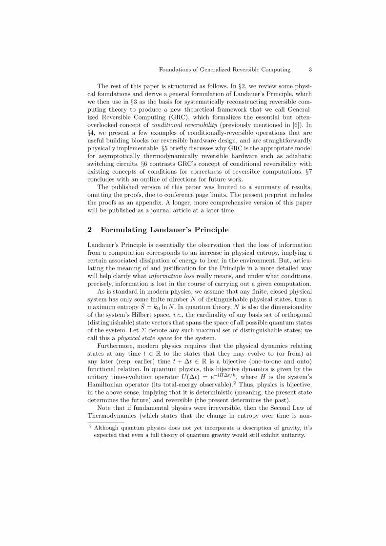
The rest of this paper is structured as follows. In §2, we review some physi-cal foundations and derive a general formulation of Landauer’s Principle, whichwe then use in §3 as the basis for systematically reconstructing reversible com-puting theory to produce a new theoretical framework that we call General-ized Reversible Computing (GRC), which formalizes the essential but often-overlooked concept of conditional reversibility (previously mentioned in [6]). In§4, we present a few examples of conditionally-reversible operations that areuseful building blocks for reversible hardware design, and are straightforwardlyphysically implementable. §5 briefly discusses why GRC is the appropriate modelfor asymptotically thermodynamically reversible hardware such as adiabaticswitching circuits. §6 contrasts GRC’s concept of conditional reversibility withexisting concepts of conditions for correctness of reversible computations. §7concludes with an outline of directions for future work.

The published version of this paper was limited to a summary of results,omitting the proofs, due to conference page limits. The present preprint includesthe proofs as an appendix. A longer, more comprehensive version of this paperwill be published as a journal article at a later time.

2 Formulating Landauer’s Principle

Landauer’s Principle is essentially the observation that the loss of informationfrom a computation corresponds to an increase in physical entropy, implying acertain associated dissipation of energy to heat in the environment. But, articu-lating the meaning of and justification for the Principle in a more detailed waywill help clarify what information loss really means, and under what conditions,precisely, information is lost in the course of carrying out a given computation.

As is standard in modern physics, we assume that any finite, closed physicalsystem has only some finite number N of distinguishable physical states, thus amaximum entropy S = kB lnN . In quantum theory, N is also the dimensionalityof the system’s Hilbert space, i.e., the cardinality of any basis set of orthogonal(distinguishable) state vectors that spans the space of all possible quantum statesof the system. Let Σ denote any such maximal set of distinguishable states; wecall this a physical state space for the system.

Furthermore, modern physics requires that the physical dynamics relatingstates at any time t ∈ R to the states that they may evolve to (or from) atany later (resp. earlier) time t + ∆t ∈ R is a bijective (one-to-one and onto)functional relation. In quantum physics, this bijective dynamics is given by theunitary time-evolution operator U(∆t) = e−iH∆t/~, where H is the system’sHamiltonian operator (its total-energy observable).2 Thus, physics is bijective,in the above sense, implying that it is deterministic (meaning, the present statedetermines the future) and reversible (the present determines the past).

Note that if fundamental physics were irreversible, then the Second Law ofThermodynamics (which states that the change in entropy over time is non-

2 Although quantum physics does not yet incorporate a description of gravity, it’sexpected that even a full theory of quantum gravity would still exhibit unitarity.

4 Michael P. Frank

negative, ∆S ≥ 0) would be false, because two distinguishable states each withnonzero probability could merge, combining their probabilities, and reducingtheir contribution to the total entropy. Thus, the reversibility of fundamentalphysics follows from the empirically-observed validity of the Second Law.

In any event, if one accepts the bijectivity of dynamical evolution as a truismof mathematical physics, then, as we will see, the validity of Landauer’s Principlefollows rigorously from it, as a theorem.

Given a physical state space Σ, a computational subspace C of Σ can beidentified with a partition of the set Σ. We say that a physical system Π is incomputational state cj ∈ C whenever there is an si ∈ cj such that the physicalstate of the system is not reliably distinguishable from si. In other words, acomputational state cj is just an equivalence class of physical states that can beconsidered equivalent to each other, in terms of the computational informationthat we are intending them to represent. We assume that we can also identifyan appropriate computational subspace C(∆t) that is a partition of the evolvedphysical state space Σ(∆t) at any past or future time t0 + ∆t ∈ R.

Consider, now, any initial-state probability distribution p0 over the completestate space Σ = Σ(0) at time t = t0. This then clearly induces an implied initialprobability distribution PI over the computational states at time t0 as well:

PI(cj) =

|cj |∑k=1

p0(sj,k), (1)

where sj,k denotes the kth physical state in computational state cj ∈ C.For probability distributions p and P over physical and computational states,

we can define corresponding entropy measures. Given any probability distribu-tion p over a physical state space Σ, the physical entropy S(p) is defined by

S(p) =

N=|Σ|∑i=1

p(si) log1

p(si), (2)

where the logarithm can be considered to be an indefinite logarithm, dimensionedin generic logarithmic units.

The bijectivity of physical dynamics then implies the following theorem:

Theorem 1. Conservation of entropy. The physical entropy of any closedsystem, as determined for any initial state distribution p0, is exactly conservedover time. I.e., if the physical entropy of an initial-state distribution p0(si) attime t0 is S(0), and we evolve that system over an elapsed time ∆t ∈ R accordingto its bijective dynamics, the physical entropy S(∆t) of its final-state probabilitydistribution p∆t at time t0 + ∆t will be the exact same value, S(∆t) = S(0).

Theorem 1 takes an ideal, theoretical perspective. In practice, entropy fromany real observer’s perspective increases, because the observer does not haveexact knowledge of the dynamics, or the capability to track it exactly. But inprinciple, the ideal perspective with constant entropy still always exists.

Foundations of Generalized Reversible Computing 5

We can also define the entropy of the computational state. Given any proba-bility distribution P over a computational state space C, the information entropyor computational entropy H(P ) is defined by:

H(P ) =

|C|∑j=1

P (cj) log1

P (cj), (3)

which, like S(p), is dimensioned in arbitrary logarithmic units.

Finally, we define the non-computational entropy as the remainder of thetotal physical entropy, other than the computational part; Snc = S − H ≥ 0.This is the expected physical entropy conditioned on the computational state.

The above definitions let us derive Landauer’s Principle, in its most general,quantitative form, as well as another form frequently seen in the literature.

Theorem 2. Landauer’s Principle (general formulation). If the compu-tational state of a system at initial time t0 has entropy HI = H(PI), and we allowthat system to evolve, according to its physical dynamics, to some other “final”time t0 + ∆t, at which its computational entropy becomes HF = H(PF) wherePF = P (∆t) is the induced probability distribution over the computational stateset C(∆t) at time t0 + ∆t, then the non-computational entropy is increased by

∆Snc = HI −HF. (4)

Conventional digital devices are typically designed to locally reduce com-putational entropy, e.g., by erasing or destructively overwriting “unknown” oldbits obliviously, i.e., ignoring any independent knowledge of their previous value.Thus, typical device operations necessarily eject entropy into the non-computa-tional form, and so, over time, non-computational entropy typically accumulatesin the system, manifesting as heating. But, systems cannot tolerate indefiniteentropy build-up without overheating. So, the entropy must ultimately be movedout to some external environment at some temperature T , which involves thedissipation of energy ∆Ediss = T∆Snc to the form of heat in that environment,by the definition of thermodynamic temperature. From Theorem 2 together withthese facts and the logarithmic identity 1 bit = (1 nat)/ log2 e = kB ln 2 followsthe more commonly-seen statement of Landauer’s Principle:

Corollary 1. Landauer’s Principle (common form). For each bit’s worthof computational information that is lost within a computer (e.g., by obliviouslyerasing or destructively overwriting it), an amount of energy

∆Ediss = kBT ln 2 (5)

must eventually be dissipated to the form of heat added to some environmentat temperature T .

6 Michael P. Frank

3 Reformulating Reversible Computing Theory

We now carefully analyze the implications of the general Landauer’s Principle(Theorem 2) for computation, and reformulate reversible computing theory onthat basis. We begin by redeveloping the foundations of the traditional the-ory of unconditionally logically-reversible operations, using a language that wesubsequently build upon to develop the generalized theory.

For our purposes, a computational device D will simply be any physicalartifact that is capable of carrying out one or more different computational op-erations, by which the physical and computational state spaces Σ,C associatedwith D’s local state are transformed. If D has an associated local computationalstate space CI = {cI1, ..., cIm} at some initial time t0, a computational operationO on D that is applicable at t0 is specified by giving a probabilistic transitionrule, i.e., a stochastic map from the initial computational state at t0 to the finalcomputational state at some later time t0 + ∆t (with ∆t > 0) by which theoperation will have been completed. Let the computational state space at thislater time be CF = {cF1, ..., cFn}. Then, the operation O : CI → P(CF) is amap from CI to probability distributions over CF; which is characterizable, interms of random variables cI, cF for the initial and final computational states,by a conditional probabilistic transition rule

ri(j) = Pr(cF = cFj | cI = cIi) = [O(cIi)](cFj), (6)

where i ∈ {1, ...,m} and j ∈ {1, ..., n}. That is, ri(j) denotes the conditionalprobability that the final computational state is cFj , given that the initial com-putational state is cIi.

A computational operation O will be called deterministic if and only if all ofthe probability distributions ri are single-valued. I.e., for each possible value ofthe initial-state index i ∈ {1, ...,m}, there is exactly one corresponding value ofthe final-state index j such that ri(j) > 0, and thus, for this value of j, it mustbe the case that ri(j) = 1, while ri(k) = 0 for all other k 6= j. If an operation Ois not deterministic, we call it nondeterministic.3 For a deterministic operationO, we can write O(cIi) to denote the unique cFj such that ri(j) = 1, that is,treating O as a simple transition function rather than a stochastic one.

A computational operation O will be called (unconditionally logically) re-versible if and only if all of the probability distributions ri have non-overlappingnonzero ranges. In other words, for each possible value of the final-state indexj ∈ {1, ..., n}, there is at most one corresponding value of the initial-state indexi such that ri(j) > 0, while rk(j) = 0 for all other k 6= i. If an operation O isnot reversible, we call it irreversible.

3 Note that this is a different sense of the word “nondeterministic” than is commonlyused in computational complexity theory, when referring to, for example, nondeter-ministic Turing machines, which conceptually evaluate all of their possible futurecomputational trajectories in parallel. Here, when we use the word “nondeterminis-tic,” we mean it simply in the physicist’s sense, to refer to randomizing or stochasticoperations; i.e., those whose result is uncertain.

Foundations of Generalized Reversible Computing 7

For a computational operation O with an initial computational state spaceCI, a (statistical) operating context for that operation is any probability distri-bution PI over the initial computational states; for any i ∈ {1, ...,m}, the valueof PI(cIi) gives the probability that the initial computational state is cIi.

A computational operation O will be called (potentially) entropy-ejecting ifand only if there is some operating context PI such that, when the operationO is applied within that context, the increase ∆Snc in the non-computationalentropy required by Landauer’s Principle is greater than zero. If an operation Ois not potentially entropy-ejecting, we call it non-entropy-ejecting.

Now, we can derive Landauer’s original result stating that only operationsthat are logically reversible (in his sense) can always avoid ejecting entropy fromthe computational state (independently of the operating context).

Theorem 3. Fundamental Theorem of Traditional Reversible Comput-ing. Non-entropy-ejecting deterministic operations must be reversible. That is,if a given deterministic computational operation O is non-entropy-ejecting, thenit is reversible in the sense defined above (its transition relation is injective).

The proof of the theorem involves showing that entropy is ejected whenstates with nonzero probability are merged by an operation. However, whenstates having zero probability are merged with other states, there is no increasein entropy. This is the key realization that sets us up to develop GRC.

To do this, we define a notion of a computation that fixes a specific sta-tistical operating context for a computational operation, and then we examinethe detailed requirements for a given computation to be non-entropy-ejecting.This leads to the concept of conditional reversibility , which is the most generalconcept of logical reversibility, and provides the appropriate foundation for GRC.

For us, a computation C = (O,PI) performed by a device D is defined byspecifying both a computational operation O to be carried out by that device, anda specific operating context PI under which the operation O is to be performed.

A computation C = (O,PI) is called (specifically) entropy-ejecting if andonly if, when the operation O is applied within the specific operating contextPI, the increase ∆Snc in the non-computational entropy required by Landauer’sPrinciple is greater than zero. If C is not specifically entropy-ejecting, we call itnon-entropy-ejecting.

A deterministic computational operation O is called conditionally reversibleif and only if there is a non-empty subset A ⊆ CI of initial computational states(the assumed set or assumed precondition) that O’s transition rule maps ontoan equal-sized set B ⊆ CF of final states. That is, each cIi ∈ A maps, one to one,to a unique cFj ∈ B where ri(j) = 1. We say that B is the image of A under O.We also say that O is (conditionally) reversible under the precondition (that theinitial state is in) A.

It turns out that all deterministic computational operations are, in fact,conditionally reversible, under some sufficiently-restrictive preconditions.

Theorem 4. Conditional reversibility of all deterministic operations.All deterministic computational operations are conditionally reversible.

8 Michael P. Frank

A trivial proof of Theorem 4 (see Appendix) involves considering preconditionsets A that are singletons. However, deterministic operations with any numberk > 1 of reachable final computational states are also conditionally reversibleunder at least one precondition set A of size k.

Whenever we wish to fix a specific assumed precondition A for the reversibil-ity of a conditionally-reversible operation O, we use the following concept:

Let O be any conditionally-reversible computational operation, and let A beany one of the preconditions under which O is reversible. Then the conditionedreversible operation OA = (O,A) denotes the concept of performing operationO in the context of a requirement that precondition A is satisfied.

Restricting the set of initial states that may have nonzero probability to aspecific proper subset A ⊂ CI represents a change to the semantics of an opera-tion, so generally, a conditioned reversible version of an arbitrary deterministicoperation is, in effect, not exactly the same operation. But we will see thatarbitrary computations can still be composed out of these restricted operations.

The central result of GRC theory (Theorem 5, below) is then that a deter-ministic computation C = (O,PI) is specifically non-entropy-ejecting, and there-fore avoids any requirement under Landauer’s Principle to dissipate any energy∆Ediss > 0 to its thermal environment, if and only if its operating context PI

assigns total probability 1 to some precondition A under which its computa-tional operation O is reversible. Moreover (Theorem 6), even if the probabilityof satisfying some such precondition only approaches 1, this is sufficient for theentropy ejected (and energy dissipation required) to approach zero.

Theorem 5. Fundamental Theorem of Generalized Reversible Com-puting. Any deterministic computation is non-entropy-ejecting if and only if atleast one of its preconditions for reversibility is satisfied. I.e., let C = (O,PI)be any deterministic computation (i.e., any computation whose operation O isdeterministic). Then, part (a): If there is some precondition A under which Ois reversible, such that A is satisfied with certainty in the operating context PI,then C is a non-entropy-ejecting computation. And, part (b): Alternatively, if nosuch precondition A is satisfied with certainty, then C is entropy-ejecting.

Theorem 6. Entropy ejection vanishes as precondition certainty ap-proaches unity. Let O be any deterministic operation, and let A be any pre-condition under which O is reversible, and let PI1, PI2, ... be any sequence ofoperation contexts for O within which the total probability mass assigned to Aapproaches 1. Then, in the corresponding sequence of computations, the entropyejected ∆Snc approaches 0.

A numerical example illustrating how the ∆Snc calculation comes out in aspecific case where the probability of violating the precondition for reversibilityis small can be found in [7].

It’s important to note that in order for real hardware devices to apply The-orems 5 and 6 to avoid or reduce energy dissipation in practice, the device mustbe designed with implicit knowledge of not only what conditionally-reversible

Foundations of Generalized Reversible Computing 9

operation it should perform, but also which specific one of the preconditions forthat operation’s reversibility it should assume is satisfied.

As we saw in Theorem 4, any deterministic computational operation O is con-ditionally reversible with respect to any given one A of its suitable preconditionsfor reversibility. For any computation C = (O,PI) that satisfies the conditionsfor reversibility of the conditioned reversible operation OA with certainty, wecan undo the effect of that computation exactly by applying any conditionedreversible operation that is what we call a reversal of OA. The reversal of aconditioned reversible operation is simply an operation that maps the image ofthe assumed set back onto the assumed set itself in a way that exactly invertsthe original forward map.

The above framework can also be extended to work with nondeterministiccomputations. In fact, adding nondeterminism to an operation only makes iteasier to avoid ejecting entropy to the non-computational state, since nondeter-minism tends to increase the computational entropy, and thus tends to reducethe non-computational entropy. As a result, a nondeterministic operation can benon-entropy-ejecting (or even entropy-absorbing, i.e., with ∆Snc < 0) even inoperating contexts where none of its preconditions for reversibility are satisfied,so long as the reduction in computational entropy caused by its irreversibility iscompensated for by an equal or greater increase in computational entropy causedby its nondeterminism. However, we will not take the time, in the present paper,to flesh out detailed analyses of such cases.

4 Examples of Conditioned Reversible Operations

Here, we define and illustrate a number of examples of conditionally reversibleoperations (including a specification of their assumed preconditions) that com-prise natural primitives out of which arbitrary reversible algorithms may becomposed. First, we introduce some textual and graphical notations for describ-ing conditioned reversible operations.

Let the computational state space be factorizable into independent statevariables x, y, z, ..., which are in general n-ary discrete variables. A commoncase will be binary variables (n = 2). For simplicity, we assume here that thesets of state variables into which the initial and final computational state spacesare factorized are identical, although more generally this may not be the case.

Given a computational state space C that is factorizable into state variablesx, y, z, ..., and given a precondition A on the initial state defined by

A = {ci ∈ C |P (x, y, ...)}, (7)

where P (x, y, ...) is some propositional (i.e., Boolean-valued) function of thestate variables x, y, ..., we can denote a conditionally-reversible operation OA onC that is reversible under precondition A using notation like:

OpName(x, y, ... |P (x, y, ...)) (8)

10 Michael P. Frank

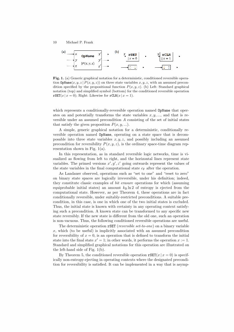
Fig. 1. (a) Generic graphical notation for a deterministic, conditioned reversible opera-tion OpName(x, y, z |P (x, y, z)) on three state variables x, y, z, with an assumed precon-dition specified by the propositional function P (x, y, z). (b) Left: Standard graphicalnotation (top) and simplified symbol (bottom) for the conditioned reversible operationrSET(x |x = 0); Right: Likewise for rCLR(x |x = 1).

which represents a conditionally-reversible operation named OpName that oper-ates on and potentially transforms the state variables x, y, ..., and that is re-versible under an assumed precondition A consisting of the set of initial statesthat satisfy the given proposition P (x, y, ...).

A simple, generic graphical notation for a deterministic, conditionally re-versible operation named OpName, operating on a state space that is decom-posable into three state variables x, y, z, and possibly including an assumedprecondition for reversibility P (x, y, z), is the ordinary space-time diagram rep-resentation shown in Fig. 1(a).

In this representation, as in standard reversible logic networks, time is vi-sualized as flowing from left to right, and the horizontal lines represent statevariables. The primed versions x′, y′, z′ going outwards represent the values ofthe state variables in the final computational state cF after the operation.

As Landauer observed, operations such as “set to one” and “reset to zero”on binary state spaces are logically irreversible, under his definition; indeed,they constitute classic examples of bit erasure operations for which (assumingequiprobable initial states) an amount kB ln 2 of entropy is ejected from thecomputational state. However, as per Theorem 4, these operations are in factconditionally reversible, under suitably-restricted preconditions. A suitable pre-condition, in this case, is one in which one of the two initial states is excluded.Thus, the initial state is known with certainty in any operating context satisfy-ing such a precondition. A known state can be transformed to any specific newstate reversibly. If the new state is different from the old one, such an operationis non-vacuous. Thus, the following conditioned reversible operations are useful.

The deterministic operation rSET (reversible set-to-one) on a binary variablex, which (to be useful) is implicitly associated with an assumed preconditionfor reversibility of x = 0, is an operation that is defined to transform the initialstate into the final state x′ = 1; in other words, it performs the operation x := 1.Standard and simplified graphical notations for this operation are illustrated onthe left-hand side of Fig. 1(b).

By Theorem 5, the conditioned reversible operation rSET(x |x = 0) is specif-ically non-entropy-ejecting in operating contexts where the designated precondi-tion for reversibility is satisfied. It can be implemented in a way that is asymp-

Foundations of Generalized Reversible Computing 11

totically physically reversible (as the probability that its precondition is satisfiedapproaches 1) using any mechanism that is designed to adiabatically transformthe state x = 0 to the state x = 1.

Similarly, we can consider a deterministic conditioned reversible operationrCLR(x |x = 1) (reversible clear or reversible reset-to-zero) which has an assumedprecondition for reversibility of x = 1 and which performs the operation x := 0,illustrated on the right-hand side of Fig. 1(b).

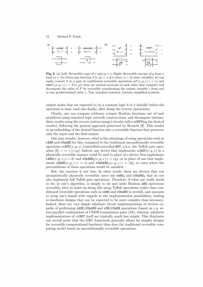
A very commonly-used computational operation is to copy one state variableto another. As with any other deterministic operation, such an operation is con-ditionally reversible under suitable preconditions. An appropriate preconditionfor the reversibility of this rCOPY operation is any in which the initial value ofthe target variable is known, so that it can be reversibly transformed to the newvalue. A standard reversal of a suitably-conditioned rCOPY operation, which wecan call rUnCOPY, is simply a conditioned reversible operation that transformsthe final states resulting from rCOPY back to the corresponding initial states.

Formally, let x, y be any two discrete state variables both with the samearity (number n of possible values, which without loss of generality we may label0, 1, ...), and let v ∈ {0, 1, ..., n − 1} be any fixed initial value. Then reversiblecopy of x onto y = v or

rCOPYv = rCOPY(x, y | y = v) (9)

is a conditioned reversible operation O with assumed precondition y = v thatmaps any initial state where x = i onto the final state x = i, y = i. In thelanguage of ordinary pseudocode, the operation performed is simply y := x.

Given any conditioned reversible copy operation rCOPYv, there is a condi-tioned reversible operation which we hereby call reversible uncopy of y from xback to v or

rUnCOPYv = rUnCOPYv(x, y | y = x) (10)

which, assuming (as its precondition for reversibility) that initially x = y, carriesout the operation y := v, restoring the destination variable y to the same initialvalue v that was assumed by the rCOPY operation.

Fig. 2(a) shows graphical notations for rCOPYv and rUnCOPYv.

It is easy to generalize rCOPY to more complex functions. In general, forany function F (x, y, ...) of any number of variables, we can define a conditionedreversible operation rF (x, y, ..., z | z = v) which computes that function, andwrites the result to an output variable z by transforming z from its initial valueto F (x, y, ...), which is reversible under the precondition that the initial value of zis some known value v. Its reversal rUnFv(x, y, ..., z | z = F (x, y, ...)) decomputesthe result in the output variable z, restoring it back to the value v. See Fig. 2(b).

The F above may indeed be any function, including standard Boolean logicfunctions operating on binary variables, such as AND, OR, etc. Therefore, the abovescheme leads us to consider conditioned reversible operations such as rAND0,rAND1, rOR0, rOR1; and their reversals rUnAND0, rUnAND1, rUnOR0, rUnOR1; whichreversibly do and undo standard AND and OR logic operations with respect to

12 Michael P. Frank

Fig. 2. (a) Left: Reversible copy of x onto y = v; Right: Reversible uncopy of y from xback to v. (b) Given any function F (x, y) = z of n (here, n = 2) state variables, we caneasily convert it to a pair of conditioned reversible operations rF (x, y, z | z = v) andrUnFv(x, y, z | z = F (x, y)) that are mutual reversals of each other that compute anddecompute the value of F by reversibly transforming the output variable z from andto any predetermined value v. Top: standard notation, bottom: simplified symbols.

output nodes that are expected to be a constant logic 0 or 1 initially before theoperation is done (and also finally, after doing the reverse operations).

Clearly, one can compose arbitrary n-input Boolean functions out of suchprimitives using standard logic network constructions, and decompute interme-diate results using the reverse (mirror-image) circuits (after rCOPYing the desiredresults), following the general approach pioneered by Bennett [8]. This resultsin an embedding of the desired function into a reversible function that preservesonly the input and the final output.

One may wonder, however, what is the advantage of using operations such asrAND and rUnAND for this, compared to the traditional unconditionally reversibleoperation ccNOT(x, y, z) (controlled-controlled-NOT, a.k.a. the Toffoli gate oper-ation [9], z := z ⊕ xy). Indeed, any device that implements ccNOT(x, y, z) in aphysically-reversible manner could be used in place of a device that implementsrAND(x, y, z | z = 0) and rUnAND0(x, y, z | z = xy), or in place of one that imple-ments rNAND(x, y, z | z = 1) and rUnNAND1(x, y, z | z = xy), in cases where thepreconditions of those operations would be satisfied.

But, the converse is not true. In other words, there are devices that canasymptotically physically reversibly carry out rAND0 and rUnAND0 that do notalso implement full Toffoli gate operations. Therefore, if what one really needsto do, in one’s algorithm, is simply to do and undo Boolean AND operationsreversibly, then to insist on doing this using Toffoli operations rather than con-ditioned reversible operations such as rAND and rUnAND is overkill, and amountsto tying one’s hands with regards to the implementation possibilities, leadingto hardware designs that can be expected to be more complex than necessary.Indeed, there are very simple adiabatic circuit implementations of devices ca-pable of performing rAND/rUnAND and rOR/rUnOR operations (based on e.g. se-ries/parallel combinations of CMOS transmission gates [10]), whereas, adiabaticimplementations of ccNOT itself are typically much less simple. This illustratesour overall point that the GRC framework generally allows for simpler designsfor reversible computational hardware than does the traditional reversible com-puting model based on unconditionally reversible operations.

Foundations of Generalized Reversible Computing 13

5 Modeling Reversible Hardware

A broader motivation for the study of GRC derives from the following observa-tion (not yet formalized as a theorem):

Assertion 1. General correspondence between truly, fully adiabatic cir-cuits and conditioned reversible operations. Part (a): Whenever a switch-ing circuit is operated deterministically in a truly, fully adiabatic way (i.e., thatasymptotically approaches thermodynamic reversibility), transitioning amongsome discrete set of logic levels, the computation being performed by that circuitcorresponds to a conditioned reversible operation OA whose assumed precondi-tion A is (asymptotically) satisfied. Part (b): Likewise, any conditioned reversibleoperation OA can be implemented in an asymptotically thermodynamically re-versible manner by using an appropriate switching circuit that is operated in atruly, fully adiabatic way, transitioning among some discrete set of logic levels.

Part (a) follows from our earlier observation in Theorem 5 that, in deter-ministic computations, conditional reversibility is the correct statement of thelogical-level requirement for avoiding energy dissipation under Landauer’s Prin-ciple, and therefore it is a necessity for approaching thermodynamic reversibilityin any deterministic computational process, and therefore, more specifically, inthe operation of adiabatic circuits.

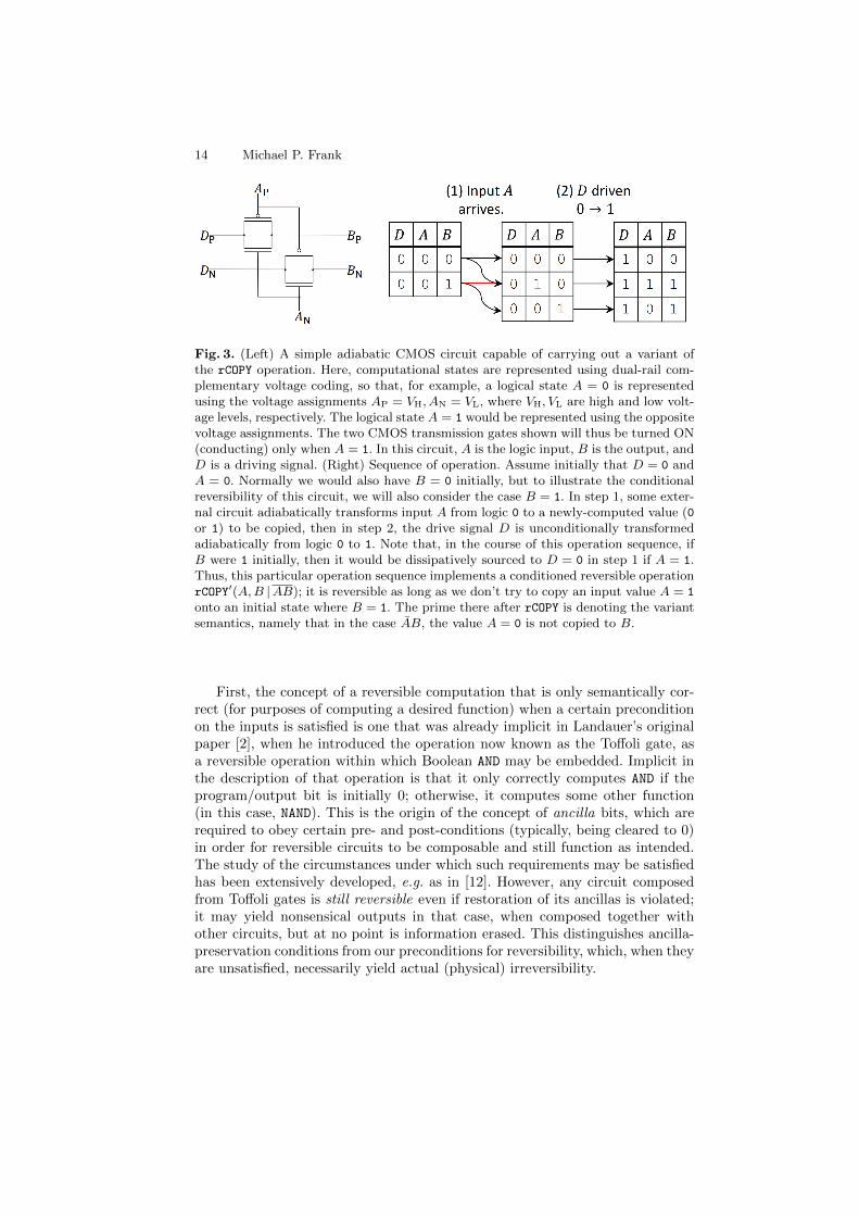
Meanwhile, part (b) follows from general constructions showing how to im-plement any desired conditioned reversible operation in an asymptotically ther-modynamically reversible way using adiabatic switching circuits. For example,Fig. 3 illustrates how to implement an rCOPY operation using a simple four-transistor CMOS circuit. In contrast, implementing rCOPY by embedding itwithin an unconditionally-reversible cNOT would require including an XOR ca-pability, and would require a much more complicated adiabatic circuit, whoseoperation would itself be composed from numerous more-primitive operations(such as adiabatic transformations of individual MOSFETs [11]) that are them-selves only conditionally reversible.

In general, the traditional reversible computing framework of uncondition-ally reversible operations does not exhibit any correspondence such as that ofAssertion 1 to any natural class of asymptotically physically-reversible hardwarethat we know of. In particular, the traditional unconditionally-reversible frame-work does not correspond to the class of truly/fully adiabatic switching circuits,because there are many such circuits that do not in fact perform unconditionallyreversible operations, but only conditionally-reversible ones.

6 Comparison to Prior Work

The concept of conditional reversibility presented here is similar to, but distinctfrom, certain concepts that are already well known in the literature on the theoryof reversible circuits and languages.

14 Michael P. Frank

Fig. 3. (Left) A simple adiabatic CMOS circuit capable of carrying out a variant ofthe rCOPY operation. Here, computational states are represented using dual-rail com-plementary voltage coding, so that, for example, a logical state A = 0 is representedusing the voltage assignments AP = VH, AN = VL, where VH, VL are high and low volt-age levels, respectively. The logical state A = 1 would be represented using the oppositevoltage assignments. The two CMOS transmission gates shown will thus be turned ON(conducting) only when A = 1. In this circuit, A is the logic input, B is the output, andD is a driving signal. (Right) Sequence of operation. Assume initially that D = 0 andA = 0. Normally we would also have B = 0 initially, but to illustrate the conditionalreversibility of this circuit, we will also consider the case B = 1. In step 1, some exter-nal circuit adiabatically transforms input A from logic 0 to a newly-computed value (0or 1) to be copied, then in step 2, the drive signal D is unconditionally transformedadiabatically from logic 0 to 1. Note that, in the course of this operation sequence, ifB were 1 initially, then it would be dissipatively sourced to D = 0 in step 1 if A = 1.Thus, this particular operation sequence implements a conditioned reversible operationrCOPY′(A,B |AB); it is reversible as long as we don’t try to copy an input value A = 1

onto an initial state where B = 1. The prime there after rCOPY is denoting the variantsemantics, namely that in the case AB, the value A = 0 is not copied to B.

First, the concept of a reversible computation that is only semantically cor-rect (for purposes of computing a desired function) when a certain preconditionon the inputs is satisfied is one that was already implicit in Landauer’s originalpaper [2], when he introduced the operation now known as the Toffoli gate, asa reversible operation within which Boolean AND may be embedded. Implicit inthe description of that operation is that it only correctly computes AND if theprogram/output bit is initially 0; otherwise, it computes some other function(in this case, NAND). This is the origin of the concept of ancilla bits, which arerequired to obey certain pre- and post-conditions (typically, being cleared to 0)in order for reversible circuits to be composable and still function as intended.The study of the circumstances under which such requirements may be satisfiedhas been extensively developed, e.g. as in [12]. However, any circuit composedfrom Toffoli gates is still reversible even if restoration of its ancillas is violated;it may yield nonsensical outputs in that case, when composed together withother circuits, but at no point is information erased. This distinguishes ancilla-preservation conditions from our preconditions for reversibility, which, when theyare unsatisfied, necessarily yield actual (physical) irreversibility.

Foundations of Generalized Reversible Computing 15

Similarly, the major historical examples of reversible high-level program-ming languages such as Janus ([13], [14]), Ψ-Lisp [15], the author’s own Rlanguage [16], and RFUN ([17], [18]) have invoked various “preconditions forreversibility” in the defined semantics of many of their language constructs.But again, that concept really has more to do with the “correctness” or “well-definedness” of a high-level reversible program, and this notion is distinct fromthe requirements for actual physical reversibility during execution. For example,the R language compiler generated PISA assembly code in such a way that evenif high-level language requirements were violated (e.g., in the case of an if con-dition changing its truth value during the if body), the resulting assembly codewould still execute reversibly, if nonsensically, on the Pendulum processor [19].

In contrast, the notion of conditional reversibility explored in the presentdocument ties directly to Landauer’s principle, and to the possibility of thephysical reversibility of the underlying hardware. Note, however, that it doesnot concern the semantic correctness of the computation, or lack thereof, and ingeneral, the necessary preconditions for the physical reversibility and correctnessof a given computation may be orthogonal to each other, as illustrated by theexample in Fig. 3.

7 Conclusion

In this paper, we presented the core foundations of a general theoretical frame-work for reversible computing. We considered the case of deterministic com-putational operations in detail, and presented results showing that the classof deterministic computations that are not required to eject any entropy fromthe computational state under Landauer’s Principle is larger than the set ofcomputations composed of the unconditionally-reversible operations consideredby traditional reversible computing theory, because it also includes the set ofconditionally-reversible operations whose preconditions for reversibility are sat-isfied with probability approaching unity. This is the most general possible char-acterization of the set of classical deterministic computations that can be phys-ically implemented in an asymptotically thermodynamically reversible way.

We then illustrated some basic applications of the theory in modeling con-ditioned reversible operations that transform an output variable between a pre-determined, known value and the computed result of the operation. Such oper-ations can be implemented easily using e.g. adiabatic switching circuits, whoselow-level computational function cannot in general be represented within thetraditional theory of unconditionally-reversible computing. This substantiatesthat the GRC theory warrants further study.

Some promising directions for future work include: (1) Giving further exam-ples of useful conditioned reversible operations; (2) illustrating detailed physicalimplementations of devices for performing such operations; (3) further extendingthe development of the new framework to address the nondeterministic case; and(4) developing further descriptive frameworks for reversible computing at higher

16 Michael P. Frank

levels (e.g., hardware description languages, programming languages) buildingon top of the fundamental conceptual foundations that GRC theory provides.

Since GRC broadens the range of design possibilities for reversible computingdevices in a clearly delineated, well-founded way, its study and further develop-ment will be essential for the computing industry to successfully transition, overthe coming decades, to the point where it is dominantly utilizing the reversiblecomputing paradigm. Due to the incontrovertible validity of Landauer’s Prin-ciple, such a transition will be an absolute physical prerequisite for the energyefficiency (and cost efficiency) of general computing technology to continue grow-ing by many orders of magnitude.

References

1. International Technology Roadmap for Semiconductors 2.0, 2015 Edition, Semicon-ductor Industry Association (2015)

2. Landauer, R.: Irreversibility and Heat Generation in the Computing Process. IBMJ. Res. Dev. 5(3), 183–191 (1961)

3. Drexler, K.E.: Nanosystems: Molecular machinery, manufacturing, and computa-tion. John Wiley & Sons, Inc. (1992)

4. Younis, S.G., Knight Jr., T.F.: Practical implementation of charge recoveringasymptotically zero power CMOS. In: Proceedings of the 1993 Symposium on Re-search in Integrated Systems, pp. 234–250. MIT Press (1993)

5. Lopez-Suarez, M., Neri, I., Gammaitoni, L.: Sub-kBT micro-electromechanical irre-versible logic gate. Nat. Comm. 7, 12068 (2016)

6. Frank, M.P.: Approaching the physical limits of computing. In: 35th InternationalSymposium on Multiple-Valued Logic, pp. 168–185. IEEE Press, New York (2005)

7. DeBenedictis, E.P., Frank, M.P., Ganesh, N., Anderson, N.G.: A path toward ultra-low-energy computing. In: IEEE International Conference on Rebooting Computing.IEEE Press, New York (2016)

8. Bennett, C.H.: Logical reversibility of computation. IBM J. Res. Dev. 17(6), 525–532(1973)

9. Toffoli, T: Reversible computing. In: International Colloquium on Automata, Lan-guages, and Programming, pp. 632–644. Springer, Berlin (1980)

10. Anantharam, V., He, M., Natarajan, K., Xie, H., Frank, M.: Driving Fully-Adiabatic Logic Circuits Using Custom High-Q MEMS Resonators. In: Arabnia,H.R., Guo, M., Yang, L.T. (eds.) ESI/VLSI 2004, pp. 5–11. CSREA Press (2004)

11. Frank, M.P.: Towards a More General Model of Reversible Logic Hardware. Invitedtalk presented at the Superconducting Electronics Approaching the Landauer Limitand Reversibility (SEALeR) workshop, sponsored by NSA/ARO (2012)

12. Thomsen, M.K., Kaarsgaard, R., Soeken, M.: Ricercar: A Language for Describingand Rewriting Reversible Circuits with Ancillae and Its Permutation Semantics. In:Krivine, J., Stefani, J.-B. (eds.) RC 2015. LNCS, vol. 9138, pp. 200-215. SpringerInternational Publishing (2015)

13. Lutz, C.: Janus: A time-reversible language. Letter from Chris Lutz to Rolf Lan-dauer, reproduced at http://tetsuo.jp/ref/janus.pdf (1986).

14. Yokoyama, T.: Reversible Computation and Reversible Programming Languages.Elec. Notes Theor. Comput. Sci. 253(6), 71–81 (2010)

Foundations of Generalized Reversible Computing 17

15. Baker, H.G.: NREVERSAL of fortune—The thermodynamics of garbage collec-tion. In: Bekkers Y., Cohen J. (eds.) Memory Management. LNCS, vol. 637, pp.507–524. Springer, Berlin, Heidelberg (1992)

16. Frank, M.: Reversibility for Efficient Computing. Doctoral dissertation, Mas-sachusetts Institute of Technology, Dept. of Elec. Eng. and Comp. Sci. (1999)

17. Yokoyama, T., Axelsen, H.B., Gluck, R.: Towards a Reversible Functional Lan-guage. In: De Vos, A., Wille, R. (eds.) RC 2011. LNCS, vol. 7165, pp. 14-29. Springer,Berlin, Heidelberg (2012)

18. Axelsen, H.B., Gluck R.: Reversible Representation and Manipulation of Construc-tor Terms in the Heap. In: Dueck, G.W., Miller, D.M. (eds.) RC 2013. LNCS, vol.7948, pp. 96-109. Springer, Berlin, Heidelberg (2013)

19. Vieri, C.J.: Reversible Computer Engineering and Architecture. Doctoral disser-tation, Massachusetts Institute of Technology, Dept. of Elec. Eng. and Comp. Sci.(1999)

Appendix: Proofs of Theorems

Proof of Theorem 1. Since the dynamical map from the state at time t0 to thestate at time t0+∆t is a one-to-one function, the probability distributions p0 andp∆t comprise the exact same bag (multiset) of real numbers (albeit reassigned tonew states); therefore, the entropy values of these distributions are identical. ut

Proof of Theorem 2. Total physical entropy is conserved by Theorem 1. Thecomputational part of the total entropy decreases by HI − HF, by hypothesis.Therefore, the noncomputational part (the remainder) must increase by thatamount. ut

Proof of Theorem 3. Suppose that O is not reversible. Then by definition itis possible to find a final-state index j such that there at least two initial stateindices (which we identify as i = 1, 2 without loss of generality) such that bothr1(j) > 0 and r2(j) > 0. Assuming that the operation is also deterministic, wemust have that r1(j) = r2(j) = 1. Thus, all of the probability mass assignedto cI1 and cI2 by the initial-state probability distribution PI will get mappedonto the same final state cFj . Therefore, if we let the operating context PI assignprobability 1/2 to each of states cI1 and cI2, then the initial computationalentropy HI = 1 bit, and the final computational entropy HF = 0, and thus theentropy ejected is ∆Snc = 1 bit. Thus, the operation O is potentially entropy-ejecting. Therefore, by contraposition, if a deterministic computational operationis non-entropy-ejecting, then it must be reversible. ut

Proof of Theorem 4. Given a deterministic computational operation O withinitial computational state space CI, (which must be non-empty, since it is apartition of a non-empty set of physical states), consider any initial computa-tional state cIi ∈ CI, and let A = {cIi}, the singleton set of state cIi. Since theoperation is deterministic, ri(j) = 1 for a single final-state index j, so then letB = {cFj}. Both A and B are the same size (both singletons), and thus O isconditionally reversible under the precondition that the initial state is in A. ut

18 Michael P. Frank

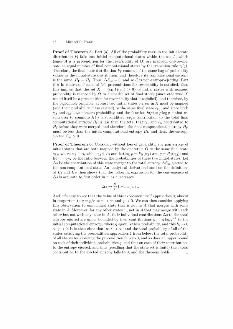
Proof of Theorem 5. Part (a): All of the probability mass in the initial-statedistribution PI falls into initial computational states within the set A, which(since A is a precondition for the reversibility of O) are mapped, one-to-one,onto an equal number of final computational states by the transition rule ri(j).Therefore, the final-state distribution PF consists of the same bag of probabilityvalues as the initial-state distribution, and therefore its computational entropyis the same, HF = HI. Thus, ∆Snc = 0, and so C is non-entropy-ejecting. Part(b): In contrast, if none of O’s preconditions for reversibility is satisfied, thenthis implies that the set X = {cIi|PI(cIi) > 0} of initial states with nonzeroprobability is mapped by O to a smaller set of final states (since otherwise Xwould itself be a precondition for reversibility that is satisfied), and therefore, bythe pigeonhole principle, at least two initial states cI1, cI2 in X must be mapped(and their probability mass carried) to the same final state cFj , and since bothcI1 and cI2 have nonzero probability, and the function h(p) = p log p−1 that wesum over to compute H(·) is subadditive, cFj ’s contribution to the total finalcomputational entropy HF is less than the total that cI1 and cI2 contributed toHI before they were merged; and therefore, the final computational entropy HF

must be less than the initial computational entropy HI, and thus, the entropyejected Snc > 0. ut

Proof of Theorem 6. Consider, without loss of generality, any pair cI1, cI2 ofinitial states that are both mapped by the operation O to the same final statecFj , where cI1 ∈ A, while cI2 /∈ A; and letting p = PI`(cI1) and q = PI`(cI2); andlet r = p/q be the ratio between the probabilities of these two initial states. Let∆s be the contribution of this state merger to the total entropy ∆Snc ejected tothe non-computational state. An analytical derivation based on the definitionsof HI and HF then shows that the following expression for the convergence of∆s is accurate to first order in r, as r increases:

∆s→ p

r(1 + ln r) nat.

And, it’s easy to see that the value of this expression itself approaches 0, almostin proportion to q = p/r as r → ∞ and q → 0. We can then consider applyingthis observation to each initial state that is not in A that merges with somestate in A. Moreover, for any other states cIi not in A that may merge with eachother but not with any state in A, their individual contributions ∆s to the totalentropy ejected are upper-bounded by their contributions hi = q log q−1 to theinitial computational entropy, where q again is their probability, and this hi → 0as q → 0. It is then clear that, as `→∞, and the total probability of all of thestates satisfying the precondition approaches 1 from below, the total probabilityof all the states violating the precondition falls to 0, and so does an upper boundon each of their individual probabilities q, and thus on each of their contributionsto the entropy ejected, and thus (recalling that the state set is finite) their totalcontribution to the ejected entropy falls to 0, and the theorem holds. ut