Embed Size (px)
Citation preview
Foundation Engineering
Prof. Mahendra Singh
Department of Civil Engineering
Indian Institute of Technology, Roorkee
Module - 03
Lecture - 10
Stability of Slopes
Hello viewers, welcome back to the lectures on Stability of Slopes, in our previous 4
lectures, we started with the infinite slopes and as discussed last time, infinite slopes are
those slopes, whose extent is very large. In general, they are the natural slopes, and the
failure surface, in those slopes were taken as parallel to the, ground surface and we had
considered, number of situations, number of conditions, and then we discussed, how to
analyze those slopes.
After that, we started discussing about the finite slopes, here it is a small extent of this
slope, finite means, it is not, that large. Generally, they are manmade structures, and we
had already, have discussions on Culmann’s method, where planar surface was
considered. And our discussions were continuing, on the planar failure surface, so we
continue with the same discussion.
(Refer Slide Time: 01:44)
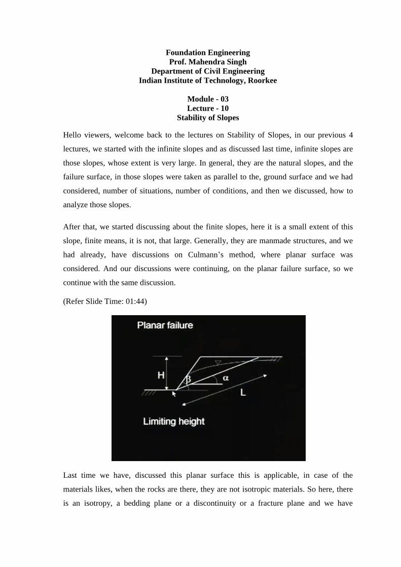
Last time we have, discussed this planar surface this is applicable, in case of the
materials likes, when the rocks are there, they are not isotropic materials. So here, there
is an isotropy, a bedding plane or a discontinuity or a fracture plane and we have
considered this, there was a water table also and this dip of the discontinuity was alpha,
angle of the slope was beta. And we discussed how to analyze this, the basic principle
remains the same, we considered the weight of this wedge and that wedge was having,
the weight was resolved into two components, normal component and tangential
components.
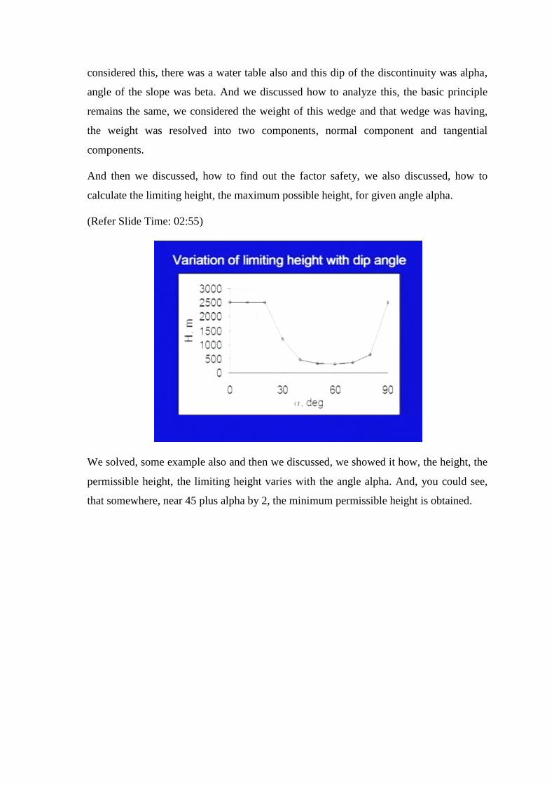
And then we discussed, how to find out the factor safety, we also discussed, how to
calculate the limiting height, the maximum possible height, for given angle alpha.
(Refer Slide Time: 02:55)
We solved, some example also and then we discussed, we showed it how, the height, the
permissible height, the limiting height varies with the angle alpha. And, you could see,
that somewhere, near 45 plus alpha by 2, the minimum permissible height is obtained.
(Refer Slide Time: 03:18)
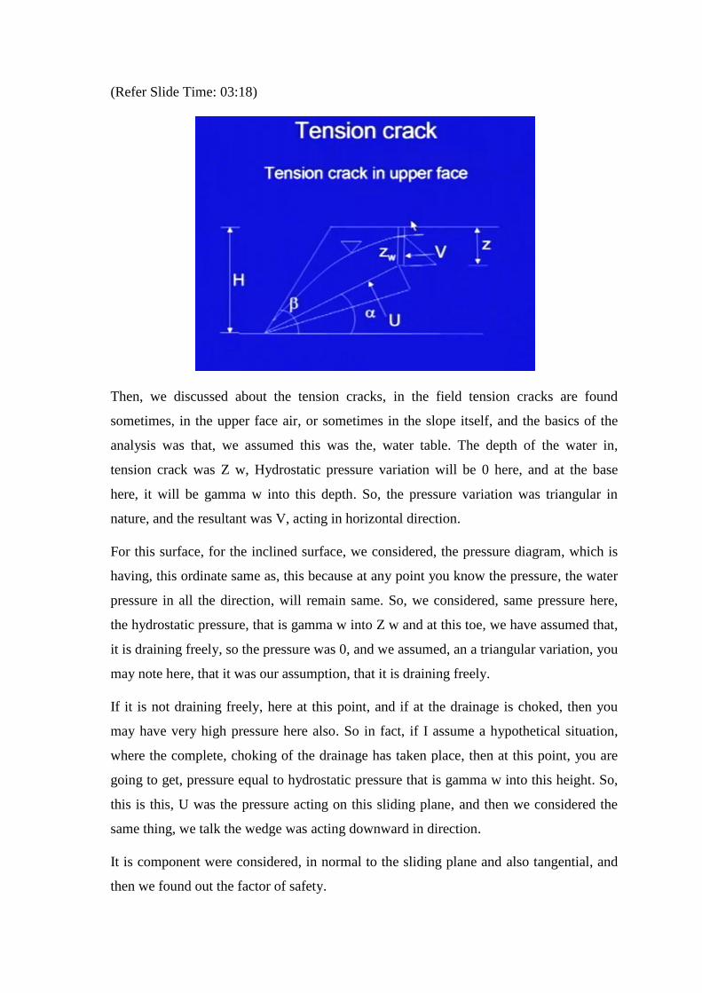
Then, we discussed about the tension cracks, in the field tension cracks are found
sometimes, in the upper face air, or sometimes in the slope itself, and the basics of the
analysis was that, we assumed this was the, water table. The depth of the water in,
tension crack was Z w, Hydrostatic pressure variation will be 0 here, and at the base
here, it will be gamma w into this depth. So, the pressure variation was triangular in
nature, and the resultant was V, acting in horizontal direction.
For this surface, for the inclined surface, we considered, the pressure diagram, which is
having, this ordinate same as, this because at any point you know the pressure, the water
pressure in all the direction, will remain same. So, we considered, same pressure here,
the hydrostatic pressure, that is gamma w into Z w and at this toe, we have assumed that,
it is draining freely, so the pressure was 0, and we assumed, an a triangular variation, you
may note here, that it was our assumption, that it is draining freely.
If it is not draining freely, here at this point, and if at the drainage is choked, then you
may have very high pressure here also. So in fact, if I assume a hypothetical situation,
where the complete, choking of the drainage has taken place, then at this point, you are
going to get, pressure equal to hydrostatic pressure that is gamma w into this height. So,
this is this, U was the pressure acting on this sliding plane, and then we considered the
same thing, we talk the wedge was acting downward in direction.
It is component were considered, in normal to the sliding plane and also tangential, and
then we found out the factor of safety.
(Refer Slide Time 05:37)
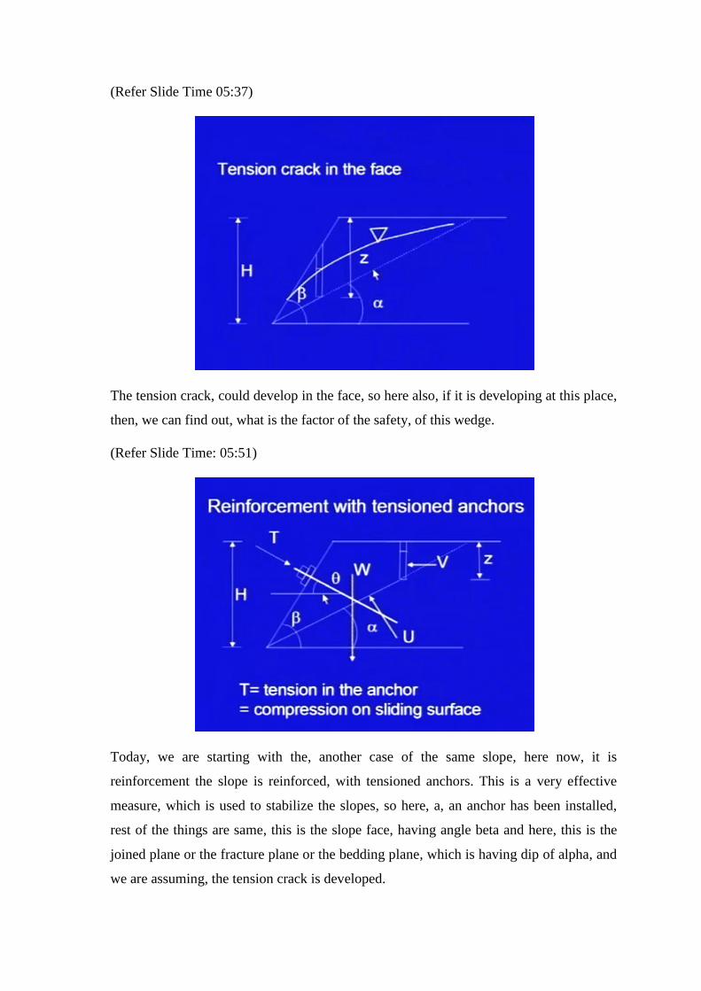
The tension crack, could develop in the face, so here also, if it is developing at this place,
then, we can find out, what is the factor of the safety, of this wedge.
(Refer Slide Time: 05:51)
Today, we are starting with the, another case of the same slope, here now, it is
reinforcement the slope is reinforced, with tensioned anchors. This is a very effective
measure, which is used to stabilize the slopes, so here, a, an anchor has been installed,
rest of the things are same, this is the slope face, having angle beta and here, this is the
joined plane or the fracture plane or the bedding plane, which is having dip of alpha, and
we are assuming, the tension crack is developed.
It is having the water pressure is V, I have not shown the water table here, so here, it is
V, same way at this inclined joined plane the water pressure acting is U, I have not
shown the complete, diagram because it might have, become very complex. So, U you
can find out, as I discussed earlier, V you can find out, W one can find out, using the
geometry of this particular wedge. And, components of W, now can be resolved, and,
and the factor of safety can be found out.
The additional force, which concern to picture at this stage is the, tension T, which is
being provided by this anchor. So, this anchor, let us say, it is inclined, at an angle theta
with horizontal, you can, see here, theta is with the horizontal, and the effect of this,
anchor will be, it is a providing force, on this sliding surface. So, here, it is increasing,
the normal component of the force, so by increasing normal component, it will enhance,
this shear strength.
So, let us say the T this is the anchor, and it is making angle theta, now you can resolve,
this force T also, perpendicular to the plane of sliding, and also tangential in the same
direction, with the plane of sliding, and then, we can do the further analysis.
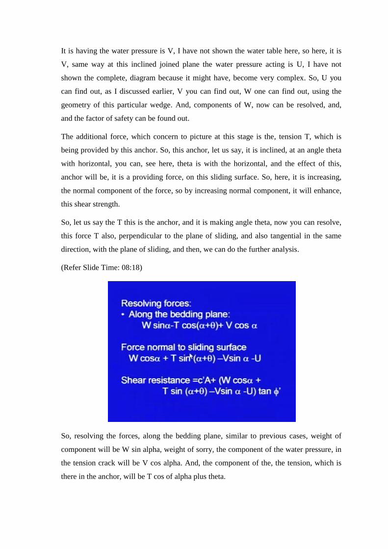
(Refer Slide Time: 08:18)
So, resolving the forces, along the bedding plane, similar to previous cases, weight of
component will be W sin alpha, weight of sorry, the component of the water pressure, in
the tension crack will be V cos alpha. And, the component of the, the tension, which is
there in the anchor, will be T cos of alpha plus theta.
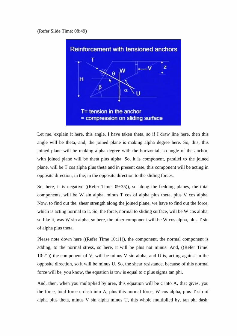
(Refer Slide Time: 08:49)
Let me, explain it here, this angle, I have taken theta, so if I draw line here, then this
angle will be theta, and, the joined plane is making alpha degree here. So, this, this
joined plane will be making alpha degree with the horizontal, so angle of the anchor,
with joined plane will be theta plus alpha. So, it is component, parallel to the joined
plane, will be T cos alpha plus theta and in present case, this component will be acting in
opposite direction, in the, in the opposite direction to the sliding forces.
So, here, it is negative ((Refer Time: 09:35)), so along the bedding planes, the total
components, will be W sin alpha, minus T cos of alpha plus theta, plus V cos alpha.
Now, to find out the, shear strength along the joined plane, we have to find out the force,
which is acting normal to it. So, the force, normal to sliding surface, will be W cos alpha,
so like it, was W sin alpha, so here, the other component will be W cos alpha, plus T sin
of alpha plus theta.
Please note down here ((Refer Time 10:11)), the component, the normal component is
adding, to the normal stress, so here, it will be plus not minus. And, ((Refer Time:
10:21)) the component of V, will be minus V sin alpha, and U is, acting against in the
opposite direction, so it will be minus U. So, the shear resistance, because of this normal
force will be, you know, the equation is tow is equal to c plus sigma tan phi.
And, then, when you multiplied by area, this equation will be c into A, that gives, you
the force, total force c dash into A, plus this normal force, W cos alpha, plus T sin of
alpha plus theta, minus V sin alpha minus U, this whole multiplied by, tan phi dash.

Here, c dash and phi dash are the shear strength, effective shear strength parameters,
now, we can find out the factor of safety.
(Refer Slide Time: 11:18)
Factor of safety is nothing but, available strength, the maximum strength, which the
sliding surface can offer. So, it will be c dash plus A, plus this entire, W cos alpha minus
U, minus V sin alpha, plus T sin theta plus alpha, times tan phi dash, divided by the
sliding force. So, it is W sin alpha, plus V cos alpha, minus T cos alpha plus theta, so this
is the final expression of the, factor of safety, and here, you can see, in this equation, if
you read, if you compare it, with the previous equation, or if you can take, T is equal to
0.
Then, what is, what is, T doing here, what is the anchor, what is the effect of providing
the anchor, you can easily analyze, using this equation. Now, due to force T you can see,
in the numerator, there is this plus term, so this is increasing, but it should be, only up to
certain value, of this theta plus alpha. So, the numerator in this expression, the numerator
is being increased, at the same time, if you look at the denominator, there is negative
quantity, so denominator is being decreased.
You are adding something in the numerator, and you are separating from something,
from the denominator, so denominator reduces, numerator increases, so there will be,
substantial increase in the factor of safety, but orientation of anchor is very important.
Because, if you want to have this, values as positive value, then theta plus alpha should
be, less than 90, if it is more than 90 degree, this quantity becomes negative, so this
becomes negative, this is also negative.
So, you may not find, any or you may find very small, increasing the factor of safety,
depending on these values. So, for positive sign, this alpha plus theta should always be
less than 90 degree, and it can be shown, that the optimal value the maximum value of
the factor of safety, will be obtained, when this expression holds good, alpha plus theta
equal to phi dash. Or, you can find out the, optimal value of theta, the inclination of the
anchor, with the horizontal, will be phi dash minus alpha.
So, if this value, if theta is equal to this much, then the optimal solution will be available,
so this is the factor of safety expression, and you can show, you can explain, why there is
so much increase in the, factor of safety.
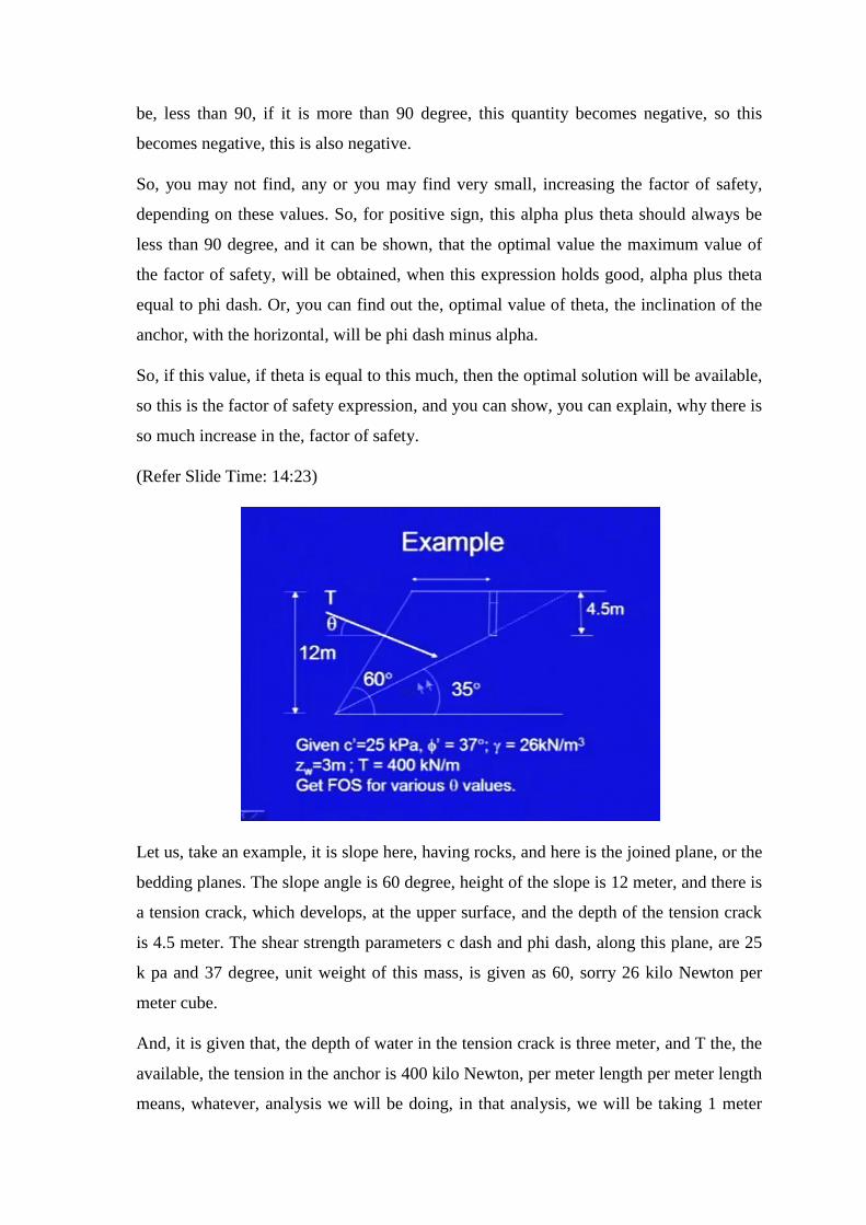
(Refer Slide Time: 14:23)
Let us, take an example, it is slope here, having rocks, and here is the joined plane, or the
bedding planes. The slope angle is 60 degree, height of the slope is 12 meter, and there is
a tension crack, which develops, at the upper surface, and the depth of the tension crack
is 4.5 meter. The shear strength parameters c dash and phi dash, along this plane, are 25
k pa and 37 degree, unit weight of this mass, is given as 60, sorry 26 kilo Newton per
meter cube.
And, it is given that, the depth of water in the tension crack is three meter, and T the, the
available, the tension in the anchor is 400 kilo Newton, per meter length per meter length
means, whatever, analysis we will be doing, in that analysis, we will be taking 1 meter
dimension, perpendicular to the plane of the paper, so per meter length, it is 400 kilo
Newton
Now, (Refer Slide Time: 15:40) we have to find out, factor of safety for various values
of theta, theta is the inclination of the anchor, with the horizontal.
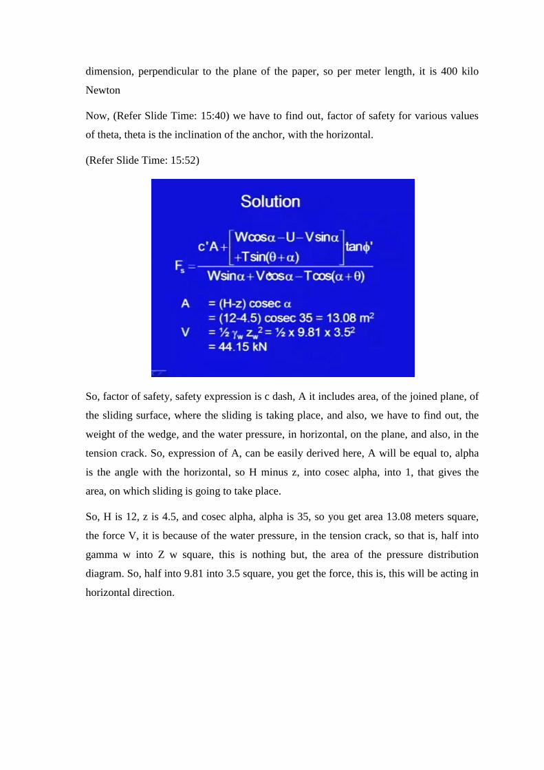
(Refer Slide Time: 15:52)
So, factor of safety, safety expression is c dash, A it includes area, of the joined plane, of
the sliding surface, where the sliding is taking place, and also, we have to find out, the
weight of the wedge, and the water pressure, in horizontal, on the plane, and also, in the
tension crack. So, expression of A, can be easily derived here, A will be equal to, alpha
is the angle with the horizontal, so H minus z, into cosec alpha, into 1, that gives the
area, on which sliding is going to take place.
So, H is 12, z is 4.5, and cosec alpha, alpha is 35, so you get area 13.08 meters square,
the force V, it is because of the water pressure, in the tension crack, so that is, half into
gamma w into Z w square, this is nothing but, the area of the pressure distribution
diagram. So, half into 9.81 into 3.5 square, you get the force, this is, this will be acting in
horizontal direction.

(Refer Slide Time: 17:11)
Also, the force on the joined plane will be area of the diagram again, and the
perpendicular ordinate, we had taken half gamma w into Z w, and the base will be, H
minus z into cosec of alpha. So, U will be half 9.81 Z w is 3, H minus z into cosec of 35,
and then you get, this value of U, T is already available, and we have been, asked to find
out different, for different theta values, what will be the factor of safety, so range of
inclination of the anchor, is within 90 degree.
We will not allow it, to increase beyond 90 degree, above that, there would not be any if
there will there will be rather the opposite fact negative fact of the anchor. So, alpha plus
theta can always be less than 90 degree, so theta, should always be less than 90 minus
35, so it can vary up to 55. Also, as I told you, though optimal expression is available
with us, so from that, for optimal value, alpha plus theta should be equal to phi dash, and
from here, theta is equal to phi dash minus alpha that comes to be equal to 2 degree.

(Refer Slide Time: 18:41)
So, now everything is available, for their expression, and simply, we have to put the
values, different angles, I have calculated only few values, 55, 30, 20 and 2. And, you
can see, the, at 55, factor of safety is 1.65, and here it is 2.10, 2.30, and 2.64, so it is, as
the theta increases, if I go from downward to upward direction, the factor of safety is
decreasing.
(Refer Slide Time: 19:16)
So, here it is theta, theta is here, so you can see, if it is almost horizontal, if this angle is
very small, 2 degree angle, then, you get the very high factor of safety. If you rotate this,
anchor, and go on increasing it, then ((Refer Time: 19:37)), you had seen that, at 55, this
is 1.65 , and In fact, if you make it inclined, further if this tan, if this anchor goes in this
direction, and T will be acting in this direction. So, it will be adding, one component of
this will be, adding to the destabilizing forces.
So, we will not allow, it to go beyond this angle, so 55 degree, secondly, you can do the
analysis, using different Z w value also. See, here, in the expression, V concern to
pictures, and V is, because of this, so you can also find out, what happens, if there is a
heavy rainfall, and this entire crack is filled with water. So, V will be maximum, or you
can also do the analysis, if there is some choke, if the drainage, at this particular toe, is
choked, what is going to happen.
So, one can, do the parametric analysis and then, you can find out, what are the
variations of the factor of safety, how the slope is going to behave, in different drainage
conditions. Drainage conditions means, for example, if this is completely choked, or it is
completely free, or here, the water the tension crack is filled with water or it is not filled
with water, it is completely dry, so the extreme values, you can find out, and then you
can have some, plan for example, during rainfall season, some warning system etcetera,
may be designed.
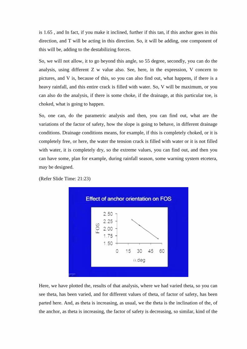
(Refer Slide Time: 21:23)
Here, we have plotted the, results of that analysis, where we had varied theta, so you can
see theta, has been varied, and for different values of theta, of factor of safety, has been
parted here. And, as theta is increasing, as usual, we the theta is the inclination of the, of
the anchor, as theta is increasing, the factor of safety is decreasing, so similar, kind of the
analysis, can be done for, different parameters for Z w, or for the drainage conditions
((Refer Time: 21:53)), the planar failure surface.
(Refer Slide Time: 22:05)
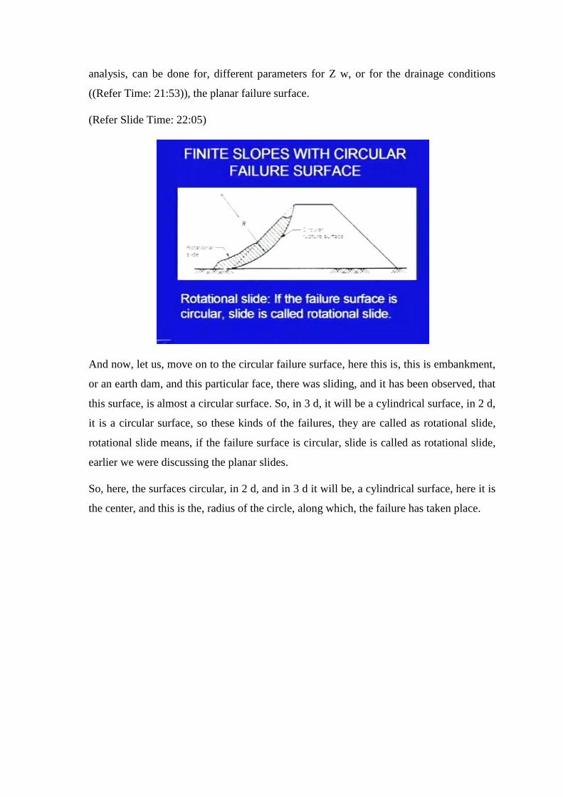
And now, let us, move on to the circular failure surface, here this is, this is embankment,
or an earth dam, and this particular face, there was sliding, and it has been observed, that
this surface, is almost a circular surface. So, in 3 d, it will be a cylindrical surface, in 2 d,
it is a circular surface, so these kinds of the failures, they are called as rotational slide,
rotational slide means, if the failure surface is circular, slide is called as rotational slide,
earlier we were discussing the planar slides.
So, here, the surfaces circular, in 2 d, and in 3 d it will be, a cylindrical surface, here it is
the center, and this is the, radius of the circle, along which, the failure has taken place.
(Refer Slide Time: 23:01)
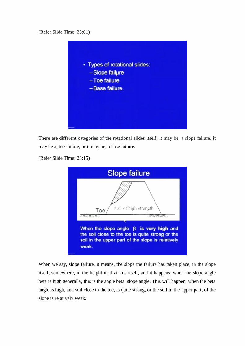
There are different categories of the rotational slides itself, it may be, a slope failure, it
may be a, toe failure, or it may be, a base failure.
(Refer Slide Time: 23:15)
When we say, slope failure, it means, the slope the failure has taken place, in the slope
itself, somewhere, in the height it, if at this itself, and it happens, when the slope angle
beta is high generally, this is the angle beta, slope angle. This will happen, when the beta
angle is high, and soil close to the toe, is quite strong, or the soil in the upper part, of the
slope is relatively weak.
So, if a composition, of this slope, of this embankment, of this manmade structure, is
something like that, that here, there is good quality of the soil, well compacted, having
higher strength, very compact very stiff, and at the top surface, it is not that compacted, it
is weaker. Then, failure can take place, in the upper surface, and this particular failure is
termed as slope failure, so here, this slope is failing.
(Refer Slide Time: 24:23)
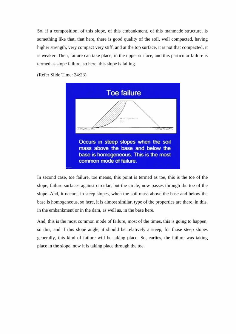
In second case, toe failure, toe means, this point is termed as toe, this is the toe of the
slope, failure surfaces against circular, but the circle, now passes through the toe of the
slope. And, it occurs, in steep slopes, when the soil mass above the base and below the
base is homogeneous, so here, it is almost similar, type of the properties are there, in this,
in the embankment or in the dam, as well as, in the base here.
And, this is the most common mode of failure, most of the times, this is going to happen,
so this, and if this slope angle, it should be relatively a steep, for those steep slopes
generally, this kind of failure will be taking place. So, earlies, the failure was taking
place in the slope, now it is taking place through the toe.

(Refer Slide Time: 25:26)
The third case, may be there, when we have stronger, soil in the embankment, or in the
dam, and in the base, here the soil is little bit softer. So, it is easy, for the failure surface
to penetrate, through the base, and in this case, the circle, the failure surface, will emerge
out of the grounds, somewhere here, which will be some distance, away from the toe. So,
it is not passing through the toe, it is little bit away, so this can occur, when the soil
below the toe is relatively weak, and soft, and the slope is also flat.
So, this generally occurs, for the flat is slopes, earlier two faces, they occur for steep
slopes, the failure circle is called midpoint circle. So, in this case the circle will be
termed as midpoint circle.
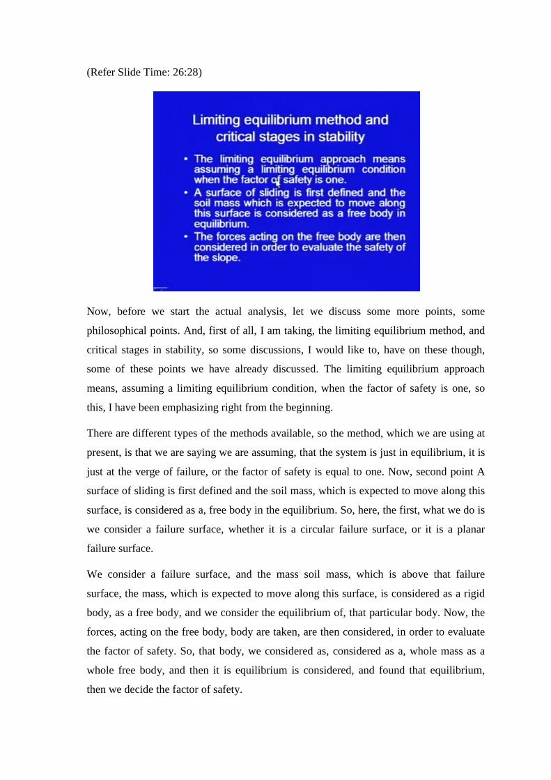
(Refer Slide Time: 26:28)
Now, before we start the actual analysis, let we discuss some more points, some
philosophical points. And, first of all, I am taking, the limiting equilibrium method, and
critical stages in stability, so some discussions, I would like to, have on these though,
some of these points we have already discussed. The limiting equilibrium approach
means, assuming a limiting equilibrium condition, when the factor of safety is one, so
this, I have been emphasizing right from the beginning.
There are different types of the methods available, so the method, which we are using at
present, is that we are saying we are assuming, that the system is just in equilibrium, it is
just at the verge of failure, or the factor of safety is equal to one. Now, second point A
surface of sliding is first defined and the soil mass, which is expected to move along this
surface, is considered as a, free body in the equilibrium. So, here, the first, what we do is
we consider a failure surface, whether it is a circular failure surface, or it is a planar
failure surface.
We consider a failure surface, and the mass soil mass, which is above that failure
surface, the mass, which is expected to move along this surface, is considered as a rigid
body, as a free body, and we consider the equilibrium of, that particular body. Now, the
forces, acting on the free body, body are taken, are then considered, in order to evaluate
the factor of safety. So, that body, we considered as, considered as a, whole mass as a
whole free body, and then it is equilibrium is considered, and found that equilibrium,
then we decide the factor of safety.
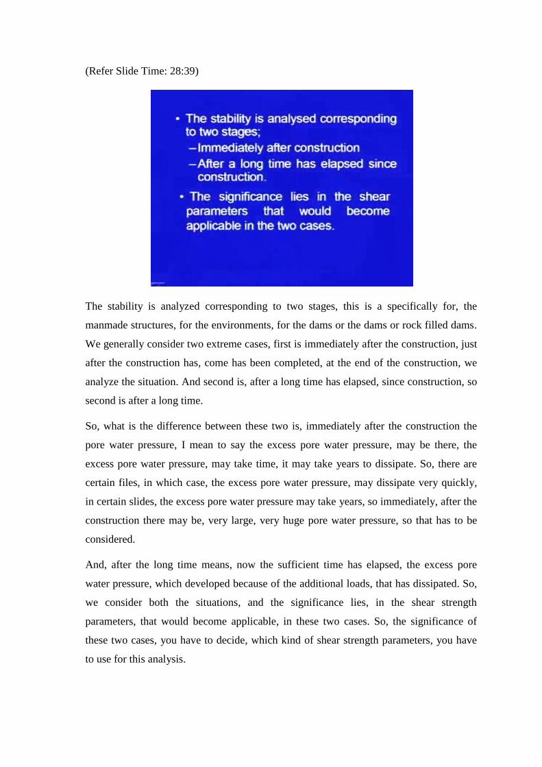
(Refer Slide Time: 28:39)
The stability is analyzed corresponding to two stages, this is a specifically for, the
manmade structures, for the environments, for the dams or the dams or rock filled dams.
We generally consider two extreme cases, first is immediately after the construction, just
after the construction has, come has been completed, at the end of the construction, we
analyze the situation. And second is, after a long time has elapsed, since construction, so
second is after a long time.
So, what is the difference between these two is, immediately after the construction the
pore water pressure, I mean to say the excess pore water pressure, may be there, the
excess pore water pressure, may take time, it may take years to dissipate. So, there are
certain files, in which case, the excess pore water pressure, may dissipate very quickly,
in certain slides, the excess pore water pressure may take years, so immediately, after the
construction there may be, very large, very huge pore water pressure, so that has to be
considered.
And, after the long time means, now the sufficient time has elapsed, the excess pore
water pressure, which developed because of the additional loads, that has dissipated. So,
we consider both the situations, and the significance lies, in the shear strength
parameters, that would become applicable, in these two cases. So, the significance of
these two cases, you have to decide, which kind of shear strength parameters, you have
to use for this analysis.
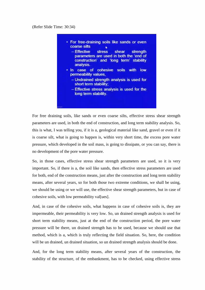
(Refer Slide Time: 30:34)
For free draining soils, like sands or even coarse silts, effective stress shear strength
parameters are used, in both the end of construction, and long term stability analysis. So,
this is what, I was telling you, if it is a, geological material like sand, gravel or even if it
is coarse silt, what is going to happen is, within very short time, the excess pore water
pressure, which developed in the soil mass, is going to dissipate, or you can say, there is
no development of the pore water pressure.
So, in those cases, effective stress shear strength parameters are used, so it is very
important. So, if there is a, the soil like sands, then effective stress parameters are used
for both, end of the construction means, just after the construction and long term stability
means, after several years, so for both those two extreme conditions, we shall be using,
we should be using or we will use, the effective shear strength parameters, but in case of
cohesive soils, with low permeability val[ues].
And, in case of the cohesive soils, what happens in case of cohesive soils is, they are
impermeable, their permeability is very low. So, un drained strength analysis is used for
short term stability means, just at the end of the construction period, the pore water
pressure will be there, un drained strength has to be used, because we should use that
method, which is a, which is truly reflecting the field situation. So, here, the condition
will be un drained, un drained situation, so un drained strength analysis should be done.
And, for the long term stability means, after several years of the construction, the
stability of the structure, of the embankment, has to be checked, using effective stress
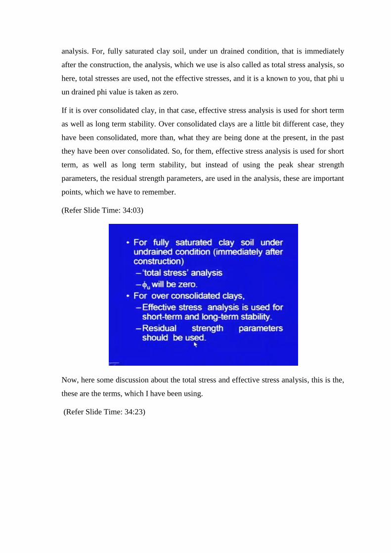
analysis. For, fully saturated clay soil, under un drained condition, that is immediately
after the construction, the analysis, which we use is also called as total stress analysis, so
here, total stresses are used, not the effective stresses, and it is a known to you, that phi u
un drained phi value is taken as zero.
If it is over consolidated clay, in that case, effective stress analysis is used for short term
as well as long term stability. Over consolidated clays are a little bit different case, they
have been consolidated, more than, what they are being done at the present, in the past
they have been over consolidated. So, for them, effective stress analysis is used for short
term, as well as long term stability, but instead of using the peak shear strength
parameters, the residual strength parameters, are used in the analysis, these are important
points, which we have to remember.
(Refer Slide Time: 34:03)
Now, here some discussion about the total stress and effective stress analysis, this is the,
these are the terms, which I have been using.
(Refer Slide Time: 34:23)
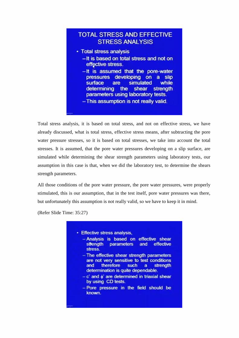
Total stress analysis, it is based on total stress, and not on effective stress, we have
already discussed, what is total stress, effective stress means, after subtracting the pore
water pressure stresses, so it is based on total stresses, we take into account the total
stresses. It is assumed, that the pore water pressures developing on a slip surface, are
simulated while determining the shear strength parameters using laboratory tests, our
assumption in this case is that, when we did the laboratory test, to determine the shears
strength parameters.
All those conditions of the pore water pressure, the pore water pressures, were properly
stimulated, this is our assumption, that in the test itself, pore water pressures was there,
but unfortunately this assumption is not really valid, so we have to keep it in mind.
(Refer Slide Time: 35:27)
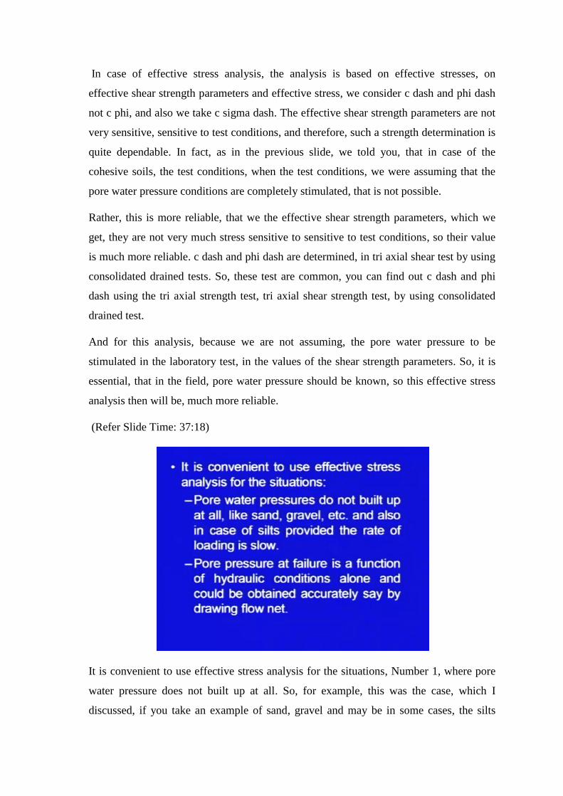
In case of effective stress analysis, the analysis is based on effective stresses, on
effective shear strength parameters and effective stress, we consider c dash and phi dash
not c phi, and also we take c sigma dash. The effective shear strength parameters are not
very sensitive, sensitive to test conditions, and therefore, such a strength determination is
quite dependable. In fact, as in the previous slide, we told you, that in case of the
cohesive soils, the test conditions, when the test conditions, we were assuming that the
pore water pressure conditions are completely stimulated, that is not possible.
Rather, this is more reliable, that we the effective shear strength parameters, which we
get, they are not very much stress sensitive to sensitive to test conditions, so their value
is much more reliable. c dash and phi dash are determined, in tri axial shear test by using
consolidated drained tests. So, these test are common, you can find out c dash and phi
dash using the tri axial strength test, tri axial shear strength test, by using consolidated
drained test.
And for this analysis, because we are not assuming, the pore water pressure to be
stimulated in the laboratory test, in the values of the shear strength parameters. So, it is
essential, that in the field, pore water pressure should be known, so this effective stress
analysis then will be, much more reliable.
(Refer Slide Time: 37:18)
It is convenient to use effective stress analysis for the situations, Number 1, where pore
water pressure does not built up at all. So, for example, this was the case, which I
discussed, if you take an example of sand, gravel and may be in some cases, the silts

also, if the pore water pressure is not developing, then if active stress analyses should be
used. It all depends on the rate of application of the load and also rate of dissipation of
pore water pressure.
So, for example, this a, this analyses effective stress analysis can be used, in case of the
silts, provided the rate of loading is slow, so if the rate of loading is slow, what is going
to happen is, the there will be some rate, at which the dissipation of pore water pressure,
excess pore water pressure, must be taking place. So, if this loading rate is slow, and the
dissipation rate is higher, it can be considered as, as dried situation, so in that case also,
this effective stress analysis is used.
Secondly, it is used where pore pressure, at failure is a function of hydraulic conditions
alone and could be obtained accurately say by drawing the flow net. So, this is important
point, we are, we are accounting for the pore water pressure separately here, by using the
effective stresses So, in the analysis, we should be able to input, we should be able to
calculate, the pore water pressure accurately. So, this is the situation, where pore water
pressure, at failure is a function of hydraulic conditions alone, so that we are able to
calculate it accurately.
For example, using the flow nets, in other words, we have to give an accurate value of
the pore water pressure, which is going to develop in the field, so these are the situations,
where the effective stress analysis can be used.
(Refer Slide Time: 39:58)
Now, let me, come to what are the different types of stability analysis procedures, we
divide them in two broad categories. One is the mass procedure and second one is the
method of slices, mass procedure means, the mass of the soil above the surface of sliding
is taken as a unit, as a we discussed earlier, we are using the limit equilibrium approach.
We will be assuming a circular failure surface, and above that, circular failure surface,
the entire mass, will be treated as a free body.
So, in this first procedure, we are treating the entire mass as a whole, and by taking it as
a whole then we will be doing the analysis. In the second method, the method of slices,
the soil above the surface of sliding is divided into number of vertical parallel slices, so
this method, you can say, it will be much more accurate in certain situations. So, here,
we are not going to take the mass as a whole, we will be dividing it into number of
vertical slices, to make our result, to make our analysis more accurate.
First we are taking the mass procedure means, the entire mass is being taken as one
body.
(Refer Slide Time: 41:25)
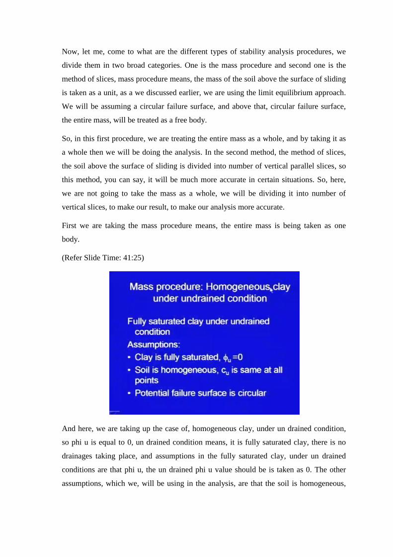
And here, we are taking up the case of, homogeneous clay, under un drained condition,
so phi u is equal to 0, un drained condition means, it is fully saturated clay, there is no
drainages taking place, and assumptions in the fully saturated clay, under un drained
conditions are that phi u, the un drained phi u value should be is taken as 0. The other
assumptions, which we, will be using in the analysis, are that the soil is homogeneous,
we have been using this, assumptions many times, and also, this shear strength
parameters C u is same, at all the points along the surface, which we have assumed.
And thirdly, the potential failure surface is being assumed to be a circle, a circular failure
surface.
(Refer Slide Time: 42:20)
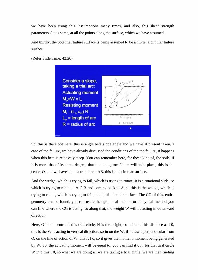
So, this is the slope here, this is angle beta slope angle and we have at present taken, a
case of toe failure, we have already discussed the conditions of the toe failure, it happens
when this beta is relatively steep. You can remember here, for these kind of, the soils, if
it is more than fifty-three degree, that toe slope, toe failure will take place, this is the
center O, and we have taken a trial circle AB, this is the circular surface.
And the wedge, which is trying to fail, which is trying to rotate, it is a rotational slide, so
which is trying to rotate is A C B and coming back to A, so this is the wedge, which is
trying to rotate, which is trying to fail, along this circular surface. The CG of this, entire
geometry can be found, you can use either graphical method or analytical method you
can find where the CG is acting, so along that, the weight W will be acting in downward
direction.
Here, O is the centre of this trial circle, H is the height, so if I take this distance as l 0,
this is the W is acting in vertical direction, so in on the W, if I draw a perpendicular from
O, on the line of action of W, this is l o, so it gives the moment, moment being generated
by W. So, the actuating moment will be equal to, you can find it out, for that trial circle
W into this l 0, so what we are doing is, we are taking a trial circle, we are then finding
out the total weight of this mass, and then we are calculating the actuating moment, that
should be equal to W into l 0.
And, what is the resisting moment, so the resistance by the soil is being offered, all along
this circular surface, so here the resistance is being offered. And, at any point, on this
periphery, the direction of the resistance, if I take this point, it will be tangential to the
circular surface. If I take this point, it will be tangential to the circular surface, if it is
here, tangential may be horizontal it is little bit in upward direction, so at every point it is
tangential, so you can find out, the sum of moments of all those small forces, which I
discussed.
So, the resisting moment will be L a, into C m, so if L a is the length of this arc, so if you
know this length of arc, which you can get, analytically very easily based on this angle
theta. You have already taken a trial circle, and this angle subtended at this center is 2
theta, radius is R, you can find out, this length of the arc, so length of the arc and
multiplied by the cohesion, this is the mobilized cohesion, so that gives you cohesive
force.
So, this force is acting all along the periphery, and it is lower arm is R, so the resisting
moment will be L a, C m into R, where L a is the length of arc, and R is the radius. So,
when it is in equilibrium, at limited equilibrium, this actuating moment and resisting
moment, they will be same, this is our assumption in the limit equilibrium method.
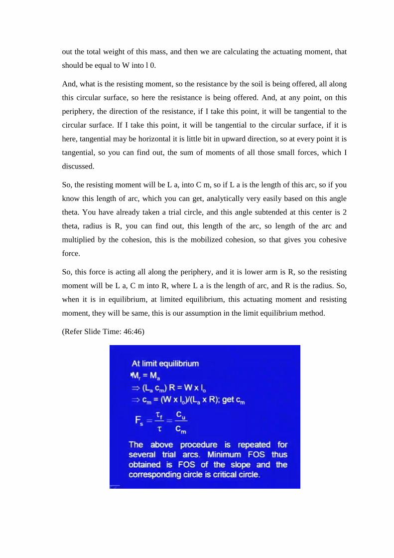
(Refer Slide Time: 46:46)
So, L A into C m into R will be equal to W into l 0, from there you can get, the
mobilized cohesion, C m is equal to W into l 0, divided by L a into capital R. So, from
this expression, you can get, that mobilized cohesion C m, which is required, to keep this
slope, instable situation, just in limit equilibrium situation, and factor of safety is defined
as, tau f upon tau, are in terms of C u and C m, you can define the factor of safety, is
always the maximum value of the cohesion, which can be offered by the soil mass and
what is the value, that is being used, that is being mobilized, to keep this slope stable.
So, F s is equal to C u upon C m, this C u will be available from the laboratory test, and
this C m will be, available from this equilibrium condition, from this mechanical
analysis. So, we will be, able to find out the factor of safety, this factor of safety, we
found for one trial circle, so this above procedure is repeated for several trial arcs,
several circles we have to assume, theoretically as it will be very large number, and then,
we have to find out the minimum, we have to find out that circle, which gives us
minimum factor of safety, and that will be considered as critical circle.
(Refer Slide Time: 48:43)
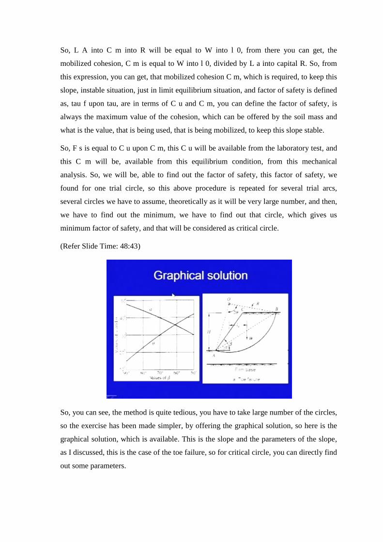
So, you can see, the method is quite tedious, you have to take large number of the circles,
so the exercise has been made simpler, by offering the graphical solution, so here is the
graphical solution, which is available. This is the slope and the parameters of the slope,
as I discussed, this is the case of the toe failure, so for critical circle, you can directly find
out some parameters.
If I take this slope here, this angle is beta, and this AB line is making angle alpha, and
here, this is an isosceles triangle A B O, which is subtending angle 2 theta at the centre,
for given beta values, here you can see, 50, 60, 70, 80 and 90, for given beta values,
these theta and alpha, can be found out, from this graphical solution. So, here on the y
axis, these are alpha and theta values and you can see, they are starting from 50 degree,
in fact, in this situation the toe failure takes place, when this beta is more than 53 degree.
So for example, suppose beta is 60, and you can go all along this line, it intersects the
alpha curve somewhere here, so you can read this value, it is somewhere between 30 and
35 or so. Same way, this theta, theta it is intersecting 60 degree line here, it is slightly
more than that, so somewhere, around 38 or so. So, corresponding to this beta, you can
get alpha and theta, once those values are available, then you can draw this line AB, you
can then, draw this triangle.
Because, this angle is 2 theta, so if I, you can very easily calculate this angle, because
this is 2 theta and it is an isosceles triangle. So, you can draw this A B O, and once this
center O is available, you can very easily, then find out the, the circle, you can very
easily draw this geometry, and you can find out w, and you can do rest of the analysis.
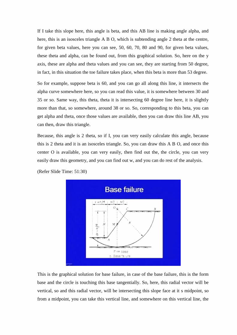
(Refer Slide Time: 51:30)
This is the graphical solution for base failure, in case of the base failure, this is the form
base and the circle is touching this base tangentially. So, here, this radial vector will be
vertical, so and this radial vector, will be intersecting this slope face at it s midpoint, so
from a midpoint, you can take this vertical line, and somewhere on this vertical line, the
somewhere near this vertical line, the exact critical circle will be there. And, these are the
parameters, and this graphical solution is noted, there will be different parameters, in
different chorographical solutions.
This is H, H is the height of the slope, and this is the firm base, so it is n d times H, from
the, this crest of the slope, so this n d into H, this is H this parameter is x, this distance is
x, this is n x into H, and here it will be B by 2, B by 2.
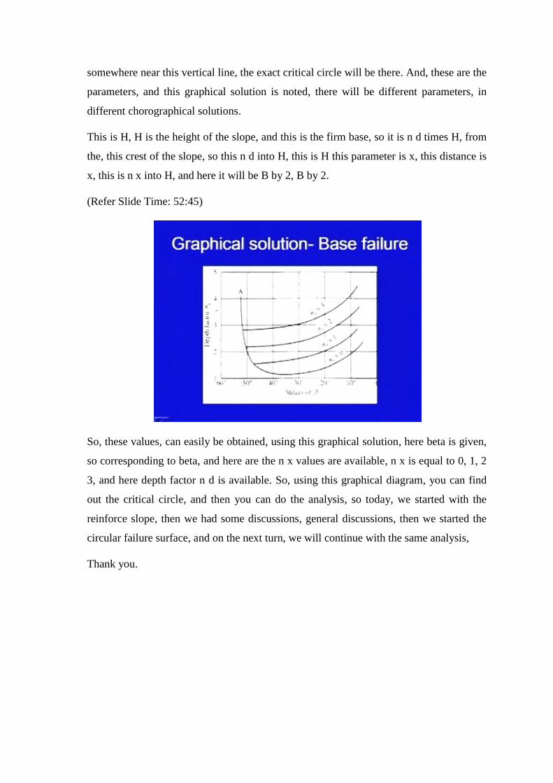
(Refer Slide Time: 52:45)
So, these values, can easily be obtained, using this graphical solution, here beta is given,
so corresponding to beta, and here are the n x values are available, n x is equal to 0, 1, 2
3, and here depth factor n d is available. So, using this graphical diagram, you can find
out the critical circle, and then you can do the analysis, so today, we started with the
reinforce slope, then we had some discussions, general discussions, then we started the
circular failure surface, and on the next turn, we will continue with the same analysis,
Thank you.