Embed Size (px)
Citation preview

Engineering Fracture Mechanics Prof. K. Ramesh
Department of Applied Mechanics Indian Institute of Technology, Madras
Module No. # 07 Lecture No. # 36
Crack Growth Models
You know, I had mentioned that, designers took to fracture mechanics, once they
realized, they could predict crack growth and also inspect, at periodic intervals. This was
made possible, with the development of Paris law. Only after Paris law was developed,
designers really looked at, linear elastic fracture mechanics is useful. And I also
mentioned, Paris law is something like a kernel, of how the crack growth takes place. He
looked at only the essentials; he did not incorporate environmental effects and several
other effects, while formulating the basic approach of Paris law. Otherwise, you would
not have got that; because the phenomenon is very very complex.
In the last class, what we saw was, one of the variations of Paris law, in the context of
crack closure. I had mentioned, when we have variable amplitude loading, you will have
to incorporate crack closure effects, while calculating the life of the component. Then,
we also had a brief look at the effect of overload. In both the cases, what you will have to
understand primarily is, because of repeated loading, there is a residual stress created,
ahead of the crack-tip. That forms a basis.

(Refer Slide Time: 01:49)
And we will again have a look at it, to understand it better. And that is what is
mentioned here. What is the residual stress ahead of a crack in a cycle. We first look at,
what happens when the load is increased from 0 to the peak load. This is the first part of
the cycle and you have the crack and the crack axis here.
(Refer Slide Time: 02:18)
And the stress field is shown like this. Along the crack axis, how does the value of
sigma y changes; it reaches a value of sigma y s.

(Refer Slide Time: 02:32)
And we all know, from the plastic zone modeling, what is the shape of the plastic zone.
And just to understand the concepts further, I show the elastically deformed material
here. So, when I increase the load from 0 to peak load, in the vicinity of the crack, you
have plastic zone developed, which is surrounded by elastic material. When you remove
the load, what will happen? The portion of the material, subjected to elastic condition
would come back to its original position. The portion, which is subjected to plastic
loading condition will also recover, by a very small amount equivalent to its elastic strain
component. Because of plastic deformation, it will have plastic strain component.
And what would eventually happen is, in the process, the elastic material, when it
recovers, it will apply excessive force in this zone; this will turn to compressive plastic
zone, which you can visualize from the way the animation is made.

(Refer Slide Time: 03:51)
.
So, what you find here is, the elastic zone has recovered and the plastic zone has been
compressed, and in the process, it is pushed to the negative part of the axis. So, what you
have is, instead of positive sigma y s, to start with, it has a residual compressive stress, in
this zone, followed by residual tension. So, what you will have to realize is, when there
is a loading and unloading, this results in formation of residual compressive stress and
tension. You know, in a normal component, when you load and unload, you do not have
residual stresses developed. In the case of a crack problem, what you find is, because of
singularity, the stresses are very high and the material has gone to the plastic zone, in the
near vicinity.
So, when you unload, you have formation of residual stresses. And this is very very
fundamental. You will not appreciate crack closure or if you will not appreciate the
retardation effect due to overload, you will have to recognize, that there would be a
residual stress, ahead of the crack-tip, because of loading and unloading; and very close
to the crack- tip, it is compressive stresses and a little distance away, you have a residual
tension.

(Refer Slide Time: 05:16)
And, this is shown for a particular amplitude. So, if we go to crack closure, what
happens. When I have several cycles this way, the crack grows; so, the plastic zone also
will increase in size and you have a plastic wake form and this wake explains, why the
crack closes before it reaches 0 load. So, you have a effective stress intensity factor is
now reduced; the change in delta K, whatever you have in an normal course of operation,
and when you have a crack closure, they are different. The delta K effective value is less
than delta K. And we had seen, how you can obtain it; people have conducted
experiments, and they have identified this. Then, people also identified different modes
of crack closure.

(Refer Slide Time: 05:16)
Once they understood plasticity induced crack closure, they moved on, to find out what
are the other mechanisms and we saw the whole range of it in the last class. Now, what
we will do is, we will move on to analyze, what happens in the case of a overload.
(Refer Slide Time: 06:58)
And you know, in fracture mechanics, influence of overload on crack growth is a very
very important aspect. And we had seen this also, in the last class, that overload in the
context of fracture mechanics is beneficial. And we have looked at two different kinds;
in one case, you have a load reversal; in another case, you have overload, only in the

positive direction. And what this graph showed was, when you have overload only in one
direction, the retardation effect is very significant.
Whereas, if I have a reversal of load, the retardation is present, but it is not that effective,
compared to the original crack growth. In fact, designers have understood it from a
different context. What they have looked at is, when they do periodic proof testing of the
pressure vessel, it has helped its life, which is nothing, but introducing overload at
periodic intervals. In proof testing, they go up to 125 percent of it; this is the field
observation. Whatever you have seen in the field, you are able to get a justification.
(Refer Slide Time: 06:58)
Then, you understand, what happens in the vicinity of the crack, because of overload.
And we would understand how the overloads, in general, retard crack growth, by looking
at the residual stress formation.

(Refer Slide Time: 08:43)
And this is done by Wheeler and he has given a model. So, what you will have to look at
is, in view of an overload, the plastic zone size is much larger. I would repeat the
animation. Here, you have a sequence of steps. And what you have here is, I have a
cyclical load here; and you have, in between the normal amplitude, an amplitude of
slightly larger in magnitude, which we will consider as a overload. So, we will look at, at
the beginning of overload, how the residual stress pattern is; after the overload, how the
residual stress pattern is; after one cycle what happens. This is what we are going to look
at. And I would like you to make a neat sketch of it. I will also increase this for your
benefit.

(Refer Slide Time: 09:41)
So, what I have here is, I have two pictures superimposed. I have a initial crack- length
a; I have a small size of the plastic zone, then I have a overload. So, because of overload,
what has happened? The crack has advanced by a length, small delta a plus you have a
larger sized plastic zone at the crack–tip. And the residual stress pattern now differs. I
have a residual compression like this, and I have a, in the earlier case, the residual
compressive stress is like this. Now, what you will have to realize is, the crack has to
come out of the larger plastic zone, introduced by the overload. During that phase, the
crack growth rate is retarded. That is the physics behind it. So, in order to appreciate this,
you will have to recognize, whenever you have a loading and unloading, residual stresses
get formed. In this case, what happens?

(Refer Slide Time: 11:03)
I have a smaller load followed by a larger load. So, for a smaller load, you have a small
sized plastic zone; for a bigger load, you have a larger plastic zone. So, after an overload,
you have only a smaller load, that is coming in the actual loading situation. So, the
smaller load, will introduce on a small size plastic zone, but this plastic zone, will remain
within the overload plastic zone.
So, as long as the crack remains within the overload plastic zone, the growth rate of the
crack would be retarded. And you also need to have, some kind of a quantitative
estimation. Here again, we will go back the Paris law and modify it. The beauty of Paris
law is, he got the kernel; others have come and modified it suitably, to take into account
for crack closure, they simply said instead of delta K, use delta K effective. In the case of
retarded crack growth, we will have a different type of model.

(Refer Slide Time: 12:11)
And, we would also have pictures, for each one of these cases. We will also see them.
So, this is the other picture you have. The subsequent crack growth is retarded due to
this, because of the overload plastic zone. And you have a picture for the ((dial also)).
So, I will zoom it for you.
(Refer Slide Time: 12:45)
So, what we are looking at is, we are looking at, after the smaller load. So, I have this,
crack has advanced, you have the smaller plastic zone, but this plastic zone, remains in
the overload plastic zone. So, the rate of crack growth will not be as high as it was

before. It is now retarded. You know, in the picture, I have shown only a smaller
increase, in the overload. Suppose, I have a larger overload, then, I would have a much
larger plastic zone. And it would also become clear, that the crack has to wade through
the larger plastic zone, because of overload. And there are certain calculations, people
do. We will have a look at it, for you to calculate the retardation.
(Refer Slide Time: 14:02)
And this is how they modified the Paris law. And, we would also a see this. I will enlarge
this for you. We will have a look at it. You have da by dN is given as phi of R multiplied
by C delta K power m. Normal Paris law would not have phi R. And phi R is defined as
delta a plus r p, 0 it is put, you take it as r p c, it is a typographical error; divided by r p
naught; you please change this, this is whole power gamma. So, what you will have is,
you will have a overload plastic zone length at the denominator and delta a plus,
whatever that you get for the cyclic, that is r p c, you put it as r p c; do not write it as r p
naught, it is a typographical error here. So, you will have a factor less than 1, which
indicates that, the growth rate is retarded. And we will also see, what is a geometric
representation of these quantities.

(Refer Slide Time: 15:20)
And, that is what is depicted here. You have along the crack axis, whatever is the length
of the overload plastic zone is given by the symbol r p overload, that is o. When you
have a normal cyclical load, the plastic zone is smaller. I think, I will try to magnify it; I
hope it comes within the screen.
(Refer Slide Time: 15:47)
So, you have it here. So, I have the definition of these terminologies. I have a small
crack length extension, because of one cycle of load; that is given as delta a. Mind you,
these are all highly exaggerated pictures. These are very very small, when you look at the

actual specimen. For the sake of clarity, they are blown up and you have to respect it that
way. So, what you have here is, at the end of overload, what is the kind of plastic zone
size you have; after the overload, only the crack and its plastic zone is shown. The earlier
graph showed, superposition of this diagram over this; now, these diagrams are drawn,
one after the other, to show the parameters. You will have delta a plus r p c.
And if you look at, the addition of delta a plus r p c would be smaller than r p naught,
and it depends on, what is the level of overload. If the overload is very high, then you
will have a larger value of r p naught, and the corresponding retardation also will be
higher. So, this is how Paris law is modeled, modified. You have a Wheelers model,
which accounts for the effect of overload.
(Refer Slide Time: 17:18)
So, as I mentioned, please make the correction in this expression. It is delta a plus r p c
divided by r p naught, where r p naught is the plastic zone length for the overload and r p
c is for the normal cycle. And this shows, when both are superimposed one over the
other, the plastic zone is still within the overload plastic zone. This causes crack to
proceed slowly. And you also have a range of what is a value of gamma, which lies
between 0 and 2 and gamma is the adjustable calibration factor. So, here again you
should appreciate, the basic kernel is Paris law, which is suitably modified to account for
retarded crack growth, which again comes in terms of what is a incremental crack length
plus the respective plastic zone sizes.

(Refer Slide Time: 18:24)
And you know, now, you will have to look at, what are the issues in fatigue crack growth
calculations. A general structure, over its life time, experiences a variable amplitude
loading. You know, this you have to keep in mind. This is unavoidable. Only from the
text book point of view, you will have a nice sinusoidal loading. When you do the
rotating bending test, you will simulate only a sinusoidal loading, which is only for
evaluating the endurance limit. In all practical structures, they experience variable
amplitude loading, which is unavoidable.
(Refer Slide Time: 19:50)

And one of the most challenging part is, how to establish a load spectrum. In the case of
ships, you find waves are battling on that, and whatever the kind of wave load, it is
highly random. It depends on the atmospheric conditions and so on and so forth; in what
speed the ship is traveling; there are many factors. So, finding out the load spectrum
itself, is a very challenging task. it is not trivial. And what you will have to keep in mind
is, the procedures for evaluating crack growth in constant amplitude, under small scale
yielding conditions, are fairly well established. I do not want to take up any other effects;
just find out the crack growth rate and I have a constant amplitude. At least, when you
want to verify your theories, you want to simulate certain tests in the laboratory, I should
have my theory predict when the failure would occur. Those kind of tests, there is no
problem.
Even in constant amplitude loading, we have seen, there could be crack closure; there
could be overload effect. If you want to include that, what way we will have to modify
the calculations. It is not simple. And that is what is summarized here.
(Refer Slide Time: 20:48)
Evaluating the geometry factor as the crack grows. See, we have looked at stress
intensity factor as K equal to beta times sigma root pi a and I said beta is the parameter
which depends on the geometry of the specimen. And, when you have a crack and the
crack starts growing, a by w ratio keeps changing. When a by w ratio keeps changing,
you will have to find out the stress intensity factor, using several terms in the series. So,

hand calculation is ruled out. In any realistic crack growth studies, if you want to go
closer to reality, you have to depend on computer programs. You cannot do hand
calculations. Hand calculations are useful, only for you to understand what equations to
use. Beyond that, they are not going to help you.
So, one of the first aspect is, as the crack grows, you will have to find out, the factor
beta, that is what is mentioned as geometry factor. Then, you have to model crack
closure; it is a very difficult task. And, also effect of overloads and in the last class, or
the previous class, we had seen the influence of the environmental conditions. When you
have a gaseous environment, or liquid environment, the crack growth rates are different.
So, how to model this. Even when you have a constant amplitude loading, these issues
are very difficult to implement. So, they pose a challenge, even in the case of constant
amplitude loading. So, you have to depend, on a sophisticated computer software and the
literature has such software. We will also have a brief look at them.
(Refer Slide Time: 22:49)
As I mentioned, variable amplitude loading is going to be very very challenging. And
what you see here is, under variable amplitude loading, similitude conditions may not be
valid. And you know, whenever we face difficulty, we will first come out with a
simplistic model. A simplistic model, if similitude conditions are assumed, can be
written as in this form. Instead of writing d a by d N, we write d a bar divided by d N;

where a bar is the average crack growth rate. And I have different cycles. I have delta K
as a function of a cycle also.
So, what you have is, you have different amplitudes; and for each of the amplitude, you
sum it like this. You have it as delta K i power m, multiplied by N i and I have total
number of cycles as N total. From this expression, you would be able to get the average
crack growth rate. It is an approximation. We will have to verify, how good this
approximation is valid, in the context of your given problem.
(Refer Slide Time: 22:49)
And obviously, for recent developments, the listener or the reader is requested to consult
advanced books on the subject and current literature in journals. There is no other go.
The usefulness of fracture mechanics is seen, only when you are able to predict crack
growth rate. But if you really want to do an analysis, simple hand calculation would not
help. For constant amplitude loading, it may give you some kind of an encouragement,
for you to understand the equations, but for any realistic calculation, you have to depend
on sophisticated software. We will also have a look at them.

(Refer Slide Time: 25:13)
So, what you have is, you have a software by NASA, which is known as NASGRO 3.0.
It was released in 2000. This was developed by the staff of the National Aeronautics and
Space Administration at Texas. You have the Johnson Space Center in Houston.
(Refer Slide Time: 25:42)
And what does this contain? The software contains three main modules; NASFLA,
NASBEM and NASMAT. And, each one performs different aspects of the whole
software package. And you have, NASFLA performs fatigue analysis. See, fatigue is a
very very involved subject. You know, there are books and handbooks written on fatigue

and how to count the number of cycles. These are all very subtle issues; you have to refer
those kind of literature.
(Refer Slide Time: 26:43)
And NASFLA encompasses all of these variables. And very complex models are listed
and these are all embedded in this. And, NASBEM performs stress analysis calculations.
And, obviously, you need to have a large material base and that is provided by
NASMAT. You know, I had already mentioned, that Paris law is an empirical relation. It
is not developed out of theory. You have data; you do a curve fitting exercise. So, for
routinely used family of materials, you need to develop exhaustive crack growth data;
from that, you find out the constants. I had also mentioned, when you have C delta K
power m, we use that in Paris law. We also use a similar form in Forman law. I had
cautioned, the same C value should not use; you should go to the material data base, and
then for that material, if Forman law is used, from that you use C and m.
So, one of the success of any of these fatigue growth calculation, depends on what
broader material data base that you have. So, the material data base is very very
important and thus specifies, for what kind of materials, you would be able to do crack
growth calculations.

(Refer Slide Time: 28:05)
And if you look at, what is the fatigue crack growth model, that they have used, in the
program, is a variation of the Forman equation.
See, we had looked at Paris law, and a modification of the Paris law for the region 3, is
given by Forman. And NASGRO, really uses a feature of this, a modification of this. I
am not getting into the equations. The crack growth rate model has considerable
flexibility to model a wide variety of materials. That is how they have chosen. The
program contains a SIF relations for a large number of crack cases. Rather than you refer
the hand book and put in the equation, you have a database; you have to just pick.
Because, this is developed by NASA, for their own use. So, an user need not know all
the nuances of how the software has been developed. At least, you should know the
limitations of the software; only then, you will be able to use it better.

(Refer Slide Time: 29:20)
So, the crack growth rate model has considerable flexibility to model a wide variety of
materials. And the program also contains SIF relations for a large number of crack cases,
that simplifies your efforts. And, it also has a large database of empirical curve-fitting
constants. See, when you go to Forman equation, when you go to modification of this,
the number of constants also may differ. So, you need to have exhaustive set of those
empirical curve fitting constants, without which, you will not able to perform a
meaningful crack growth operation and that is the…
(Refer Slide Time: 30:07)

And if you look at, what are the constituents of NASFLA module, it can provide the
following calculation options. You can do direct life predictions; the program computes
the critical flaw size; for a given initial crack size, determines the number of cycles to
failure. This is direct calculation. This is basic in any fracture mechanics calculation.
(Refer Slide Time: 30:39)
In addition to this, it also provides allowable load analysis. What the program does is, it
computes the maximum allowable load factors, to achieve a prescribed fatigue life for a
given initial and final crack sizes. So, it really helps in design. So, if you, you do not
want any component to live for infinite life; you may decide for a finite life. So, you
have a critical crack size estimated; initial crack size estimated. It tells you how much
loading you can do. So, this helps in your design scenario.

(Refer Slide Time: 30:39)
So, it can do direct life predictions, and it can also do allowable load analysis. And, what
is the third aspect that we require. We need to know how to inspect; at what periodic
intervals that you have to go and inspect. This is also possible in NASFLA.
(Refer Slide Time: 31:45)
And it does it, in a different way. You have the module for inspection limit
computations, and in this, what you do is, the program iteratively calculates the flaw
size, that will result in failure, for a given critical crack size, applied loads and the
preselected fatigue life. So, you are working backwards. You specify the failure; you

also specify the load; you also specify the cycle; you go back and calculate, what original
flaw size would precipitate this. So, this way, you would be able to decide the inspection
limits. So, it is quite comprehensive, you are able to do direct life estimation; then, you
can find out the allowable load factors; finally, you can also find the inspection limit
computations.
(Refer Slide Time: 32:43)
And you know, when you do all these calculations, you may not know what is a initial
flaw size. General practice is, depending on the NDT methodology that we use, you have
a minimum flaw size. But what this database provides is, it gives a standard of minimum
flaw sizes, acceptable for space flight hardware. Because it is developed by NASA, they
were concerned with a space program. So, they have minimum flaw sizes. And the
recommended flaw size is based on the inspection method. So, whatever the NDT
methodology that you select, it has certain inherent capabilities. You cannot go below a
certain level of the crack that you can inspect. So, the recommendation has to
incorporate, what is the method of NDT we are going to employ. So, it is a combination
of several factors. So, you do not have to worry, if you do not know, what is the initial
flaw size. The program has a database, which provides a minimum flaw sizes.

(Refer Slide Time: 35:04)
You know, you do not have only NASGRO; you also have AFGROW version 4.0; and
user manual was provided by Harter in 1999. This was developed by U.S Air Force and
what is stated is, this program is more user friendly, but less comprehensive, than
NASGRO. See, obviously, in the field, people would like to have user friendly program.
And this is developed by Air force personnel. So, it is tailor-made to aircraft industry.
So, that was tailor-made to space industry. So, that difference you will see. It uses the
data base NASMAT of NASGRO, but offers, different options for modeling fatigue.
So, this is an additional feature it has. AFGROW has some crack cases, that are more
probable to be seen in aircrafts, which are not found in NASGRO. This is quite obvious;
this is again user based. So, aircraft industry people would like to focus more on what
kind of cracks are probable, what kind of loading you anticipate in the case of aircrafts.
So, these are included as part of AFGROW. Another advantage of AFGROW is, it is
compatible with spreadsheets. So, easy to integrate in design calculations. You know, I
have some students from industry; they do not go and write a software, if they are asked
to do a design scenario. They quickly go and put the spreadsheet; they are very
comfortable with spreadsheet. They will not go near the software; and they can do all the
computations as spreadsheet. So, keeping that in mind, AFGROW is made to be
compatible with spread sheets. So, in a design office, this is a very useful tool.

(Refer Slide Time: 36:20)
And what we will say is, in summary, let us look at, what are the empirical fatigue
growth models we have seen so far. We have seen Paris law, which is the simplest. You
have a d a by d N equal to C delta K power m. Then, we had seen Donahue et al law
which accounts for the K threshold, that is regions one and two. This is given as da by
dN equal to C delta K minus delta K threshold whole power m. Then, you have the
Forman law. We saw that a variation of Forman law is used in advanced software for
crack growth calculation. This accounts for region two and region three better. And you
have da by dN equal to C delta K power n divided by 1 minus R multiplied by K C
minus delta K. Then, you have d a by d N equal to C into 1 plus beta power m multiplied
by delta K minus delta K threshold whole power n divided by K C minus 1 plus beta
multiplied by delta K; this accounts for region one, region two and region three; this is
by Erdogan and Ratwani. So, these are all the variations of basic Paris law, to account for
different regions. Then, we will also look at, how this could be modified for different
effects.
(Refer Slide Time: 38:14)
We have the crack closure introduced by Elber; you have d by, d a by d N equal to C
delta K effective whole power m. And, when you have a retardation effect, introduced by
Wheeler, you have this as d a by d N equal to phi R C delta K power m, where phi R is
the retardation parameter. Then, if we have a variable amplitude loading, you can
calculate average crack growth rate d a bar divided by d N equal to C by N total sigma 1
to n delta K i whole power m multiplied by N i. After looking at the basic Paris law,
people also have proposed, if we have very large plastic zone size, you can also calculate
d a by d N equal to C delta J power m, where J is a J integral. In fact, in the next class,
we would understand what is J.
So, these are all the modifications of the basic Paris law for different situations. So, one
of the very important aspect of this part of the course is, it provides you methodology to
find out the crack growth rate for variety of situations. You have laws, that have been
proposed by various people, and if we have the access to these empirical constants for
the material in the study, you would be able to utilize them for your life prediction
calculation. See, another important aspect that we have to understand is, how does crack
initiates. People also have done certain studies, on how does crack initiates. We will look
at that.
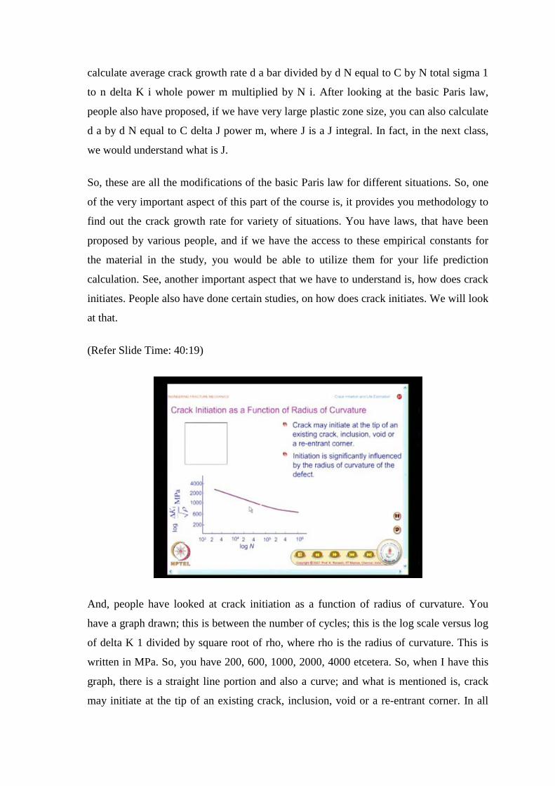
(Refer Slide Time: 40:19)
And, people have looked at crack initiation as a function of radius of curvature. You
have a graph drawn; this is between the number of cycles; this is the log scale versus log
of delta K 1 divided by square root of rho, where rho is the radius of curvature. This is
written in MPa. So, you have 200, 600, 1000, 2000, 4000 etcetera. So, when I have this
graph, there is a straight line portion and also a curve; and what is mentioned is, crack
may initiate at the tip of an existing crack, inclusion, void or a re-entrant corner. In all

these cases, initiation is significantly influenced by the radius of curvature of the defect.
And this graph shows, how does the radius of curvature acts as an influence. It will be
drawn for different values of notch radius rho; this is drawn for 0.2 millimeter; now, it is
drawn for 0.4 millimeter; it is drawn for point, 1.6 millimeter; then, it is drawn for 6
millimeter.
(Refer Slide Time: 41:39)
But what you find is, there is some variation in the initial portion; at a later portion, it all
becomes stabilized, you have something like a limit. And, you find, when the radius of
curvature is higher, which is indicated by blunt crack-tips, initiation life is high; it takes a
longer time to get initiated.
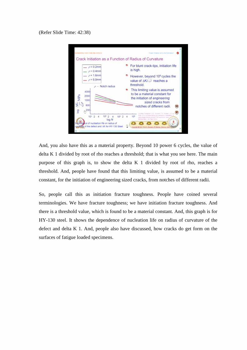
(Refer Slide Time: 42:38)
And, you also have this as a material property. Beyond 10 power 6 cycles, the value of
delta K 1 divided by root of rho reaches a threshold; that is what you see here. The main
purpose of this graph is, to show the delta K 1 divided by root of rho, reaches a
threshold. And, people have found that this limiting value, is assumed to be a material
constant, for the initiation of engineering sized cracks, from notches of different radii.
So, people call this as initiation fracture toughness. People have coined several
terminologies. We have fracture toughness; we have initiation fracture toughness. And
there is a threshold value, which is found to be a material constant. And, this graph is for
HY-130 steel. It shows the dependence of nucleation life on radius of curvature of the
defect and delta K 1. And, people also have discussed, how cracks do get form on the
surfaces of fatigue loaded specimens.

(Refer Slide Time: 43:57)
You have concepts like intrusion and extrusion. I would like you to make a reasonable
sketch of it. And this is a very highly magnified picture, to drive home the point. And
what you see here is, this is the surface of the specimen, and you have slip planes that is
projecting out of the specimen called as an extrusion; and valleys are formed, which is
called as intrusion. And this is a very highly magnified picture. And, we will also see a
support from experiment. Under fatigue loading, the surface material tends to deform by
cyclic slip in persistent slip bands, which are known as PSBs, with irregular notched
profiles, consisting of intrusion and extrusion; and these intrusions grow into a crack. So,
that means, when you have a fatigue loading, what does this slide show is, a smoothly
polished fatigue surface would become rough; because of intrusion and extrusion, which
happens at a very very small scale. It is very highly magnified for clarity.

(Refer Slide Time: 43:57)
So, the roughness of the surface should change, which you would see by an experiment.
And what you find is, the type of the intrusion, extrusion, whatever you see here, they
are different, when you have fatigue loading and when you have monotonic loading.
That is also recorded in the literature; that is what is shown here.
(Refer Slide Time: 45:54)
In monotonic loading, the slip bands are like this; in the case of fatigue loading, you have
extrusion as well as intrusion, and intrusion can eventually become a surface crack.
People have shown evidence of that. So, that is why, if you have a highly smooth fatigue
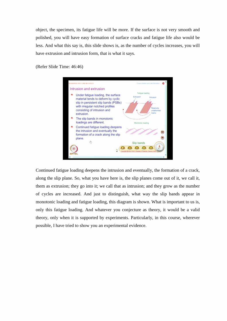
object, the specimen, its fatigue life will be more. If the surface is not very smooth and
polished, you will have easy formation of surface cracks and fatigue life also would be
less. And what this say is, this slide shows is, as the number of cycles increases, you will
have extrusion and intrusion form, that is what it says.
(Refer Slide Time: 46:46)
Continued fatigue loading deepens the intrusion and eventually, the formation of a crack,
along the slip plane. So, what you have here is, the slip planes come out of it, we call it,
them as extrusion; they go into it; we call that as intrusion; and they grow as the number
of cycles are increased. And just to distinguish, what way the slip bands appear in
monotonic loading and fatigue loading, this diagram is shown. What is important to us is,
only this fatigue loading. And whatever you conjecture as theory, it would be a valid
theory, only when it is supported by experiments. Particularly, in this course, wherever
possible, I have tried to show you an experimental evidence.

(Refer Slide Time: 47:55)
For this case also, I will show an experimental evidence, which was published in 2005.
And this is what it says, ‘in fatigue of low carbon steel, slip bands appear on the surface,
in the early stages of fatigue’. And what does the theory say? The density of the slip
bands increases, with progress of fatigue damage. We would see that as part of the
experimental result. The progress of fatigue damage as a function of number of cycles
has been recorded recently by laser diffusion technique. And I will magnify this picture.
Before I magnify, what I want to show you here is, the surface profile which was
originally smooth, has become roughened here.

(Refer Slide Time: 49:02)
And what you see here is, a diffusion pattern for the cycle 1.5 into 10 power 4. You see
white dots here, which give the diffusion pattern. This was published in 2005. And we
will see what happens, when the number of cycles is increased.
(Refer Slide Time: 49:26)
When the number of cycles increased to 12 into 10 power 4, the size of the diffusion
pattern has definitely grown. So, this is an indication, that you have, slip bands are
formed; the density of this fatigue damage increases after several cycles. So, this
explains, that cracks can form at the surface and go beneath, and then, your Paris law

comes to your rescue, to find out how the crack will grow. Crack initiation is a very
important phase. I said, this is the phase where material scientists have to work to delay
the crack initiation. And here, you see different models how crack initiates from the
surface.
(Refer Slide Time: 50:12)
So, we will again see this animation. We will see for the initial state, where you have the
surface is smooth, where N equal to 0, you hardly see anything; you just see only one
dot.
(Refer Slide Time: 50:32)

I think I can also magnify it and then show; you just see a dot.
(Refer Slide Time: 50:43)
And when the cycle is increased, you see several dots. When the cycle is further
increased, you see a large number of dots, indicating the extent of fatigue damage.
(Refer Slide Time: 50:57)
And if you look at, the corresponding surface profile, it is so wavy; it was not like this
earlier. It was, to start with, it was almost horizontal; then you saw some waviness; now,
you have very many changes on the surface.

So, in this class, what we had done was, we had looked at Wheeler’s model, to explain
the overload phenomena. And we had looked at how retardation can be calculated. Then,
I said, for any meaningful calculation of life, you will have to depend on computer
software; because, even estimation of stress intensity factor as the crack grows, we will
have to bring in geometry factor; only then the calculation is accurate. Then, you have to
bring in crack closure effects; then, you have to bring in overload effects as well as the
environment. So, it is better, that you go and look for softwares that are available. One is
by NASGRO, published by NASA. There is another one done by US Air Force, which is
called as AFGROW. Then, we looked at, how does crack initiate. We have seen, it is a
function of the radius of curvature and there is a initiation threshold, which is a material
constant. Then, we also looked at, intrusion and extrusion, which says how cracks can
form on the surface and go deeper and fatigue damage can result. Thank you.


![[OS 213] LEC36 CVS Course Summary](https://img.pdfslide.us/doc/110x75/563db911550346aa9a99b1ef/os-213-lec36-cvs-course-summary.jpg)
