Formation of telluric planets and the origin of terrestrial water

Sean Raymond1,a

1Laboratoire d’Astrophysique de Bordeaux, UMR 5804

Abstract. Simulations of planet formation have failed to reproduce Mars’ small mass(compared with Earth) for 20 years. Here I will present a solution to the Mars problemthat invokes large-scale migration of Jupiter and Saturn while they were still embedded inthe gaseous protoplanetary disk. Jupiter first migrated inward, then "tacked" and migratedback outward when Saturn caught up to it and became trapped in resonance. If this tackoccurred when Jupiter was at 1.5 AU then the inner disk of rocky planetesimals and em-bryos is truncated and the masses and orbits of all four terrestrial planet are quantitativelyreproduced. As the giant planets migrate back outward they re-populate the asteroid beltfrom two different source populations, matching the structure of the current belt. C-typematerial is also scattered inward to the terrestrial planet-forming zone, delivering aboutthe right amount of water to Earth on 10-50 Myr timescales.

1 Introduction

2 The formation of terrestrial planets

As described in the Introduction, the final stages of terrestrial planet formation take place in thepresence of any giant planets that may have formed. In addition, it is during this phase that bodies arelarge enough that during gravitational close encounters they can obtain large eccentricities. Thus, thefeeding zones of the terrestrial planets are determined during their final accretion. The compositionof each planet is simply a massweighted combination of the initial composition of all the material inits feeding zone.The inner Solar System is thought to have been too hot to allow water to condense [1], [2]. Thus,it is widely thought that Earth’s local building blocks were dry and that water was "delivered" viaimpacts from objects that condensed at cooler temperatures. Earth’s water is a chemical match tocarbonaceous chondrite meteorites (fragments of C-type asteroids) in terms of D/H and other isotopicratios [3], [4].

Simulations like the one illustrated in figure 2 above have the attractive feature of explaining theorigin of Earth’s water [6], [7], [5], [8]. In such simulations the feeding zones of the terrestrial planetsspread outward and widen in time such that a fraction of the Earth’s component mass originated inthe outer asteroid belt, beyond 3 AU. The material that originated in that cold location thus representsthe source of water on Earth in that model. This water-rich material slowly diffuses inward during

ae-mail: sean.raymond@obs.u-bordeaux1.fr

DOI: 10.1051/C© Owned by the authors, published by EDP Sciences, 2014

,/

01003 (2014)20140201003

2BIO Web of Conferencesbioconf

This is an Open Access article distributed under the terms of the Creative Commons Attribution License 2.0, which permits unrestricted use, distribution, and reproduction in any medium, provided the original work is properly cited

Article available at http://www.bio-conferences.org or http://dx.doi.org/10.1051/bioconf/20140201003

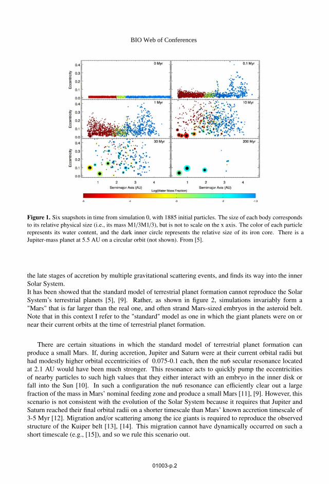
Figure 1. Six snapshots in time from simulation 0, with 1885 initial particles. The size of each body corresponds to its relative physical size (i.e., its mass M1/3M1/3), but is not to scale on the x axis. The color of each particle represents its water content, and the dark inner circle represents the relative size of its iron core. There is a Jupiter-mass planet at 5.5 AU on a circular orbit (not shown). From [5].

the late stages of accretion by multiple gravitational scattering events, and finds its way into the innerSolar System.It has been showed that the standard model of terrestrial planet formation cannot reproduce the SolarSystem’s terrestrial planets [5], [9]. Rather, as shown in figure 2, simulations invariably form a"Mars" that is far larger than the real one, and often strand Mars-sized embryos in the asteroid belt.Note that in this context I refer to the "standard" model as one in which the giant planets were on ornear their current orbits at the time of terrestrial planet formation.

There are certain situations in which the standard model of terrestrial planet formation canproduce a small Mars. If, during accretion, Jupiter and Saturn were at their current orbital radii buthad modestly higher orbital eccentricities of 0.075-0.1 each, then the nu6 secular resonance locatedat 2.1 AU would have been much stronger. This resonance acts to quickly pump the eccentricitiesof nearby particles to such high values that they either interact with an embryo in the inner disk orfall into the Sun [10]. In such a configuration the nu6 resonance can efficiently clear out a largefraction of the mass in Mars’ nominal feeding zone and produce a small Mars [11], [9]. However, thisscenario is not consistent with the evolution of the Solar System because it requires that Jupiter andSaturn reached their final orbital radii on a shorter timescale than Mars’ known accretion timescale of3-5 Myr [12]. Migration and/or scattering among the ice giants is required to reproduce the observedstructure of the Kuiper belt [13], [14]. This migration cannot have dynamically occurred on such ashort timescale (e.g., [15]), and so we rule this scenario out.

BIO Web of Conferences

01003-p.2

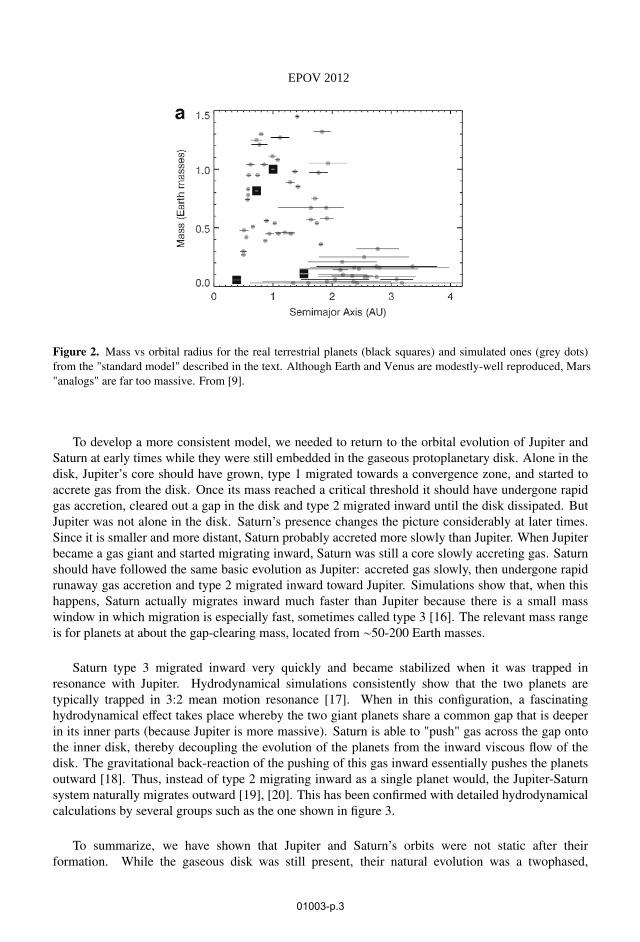
Figure 2. Mass vs orbital radius for the real terrestrial planets (black squares) and simulated ones (grey dots) from the "standard model" described in the text. Although Earth and Venus are modestly-well reproduced, Mars "analogs" are far too massive. From [9].

To develop a more consistent model, we needed to return to the orbital evolution of Jupiter andSaturn at early times while they were still embedded in the gaseous protoplanetary disk. Alone in thedisk, Jupiter’s core should have grown, type 1 migrated towards a convergence zone, and started toaccrete gas from the disk. Once its mass reached a critical threshold it should have undergone rapidgas accretion, cleared out a gap in the disk and type 2 migrated inward until the disk dissipated. ButJupiter was not alone in the disk. Saturn’s presence changes the picture considerably at later times.Since it is smaller and more distant, Saturn probably accreted more slowly than Jupiter. When Jupiterbecame a gas giant and started migrating inward, Saturn was still a core slowly accreting gas. Saturnshould have followed the same basic evolution as Jupiter: accreted gas slowly, then undergone rapidrunaway gas accretion and type 2 migrated inward toward Jupiter. Simulations show that, when thishappens, Saturn actually migrates inward much faster than Jupiter because there is a small masswindow in which migration is especially fast, sometimes called type 3 [16]. The relevant mass rangeis for planets at about the gap-clearing mass, located from ∼50-200 Earth masses.

Saturn type 3 migrated inward very quickly and became stabilized when it was trapped inresonance with Jupiter. Hydrodynamical simulations consistently show that the two planets aretypically trapped in 3:2 mean motion resonance [17]. When in this configuration, a fascinatinghydrodynamical effect takes place whereby the two giant planets share a common gap that is deeperin its inner parts (because Jupiter is more massive). Saturn is able to "push" gas across the gap ontothe inner disk, thereby decoupling the evolution of the planets from the inward viscous flow of thedisk. The gravitational back-reaction of the pushing of this gas inward essentially pushes the planetsoutward [18]. Thus, instead of type 2 migrating inward as a single planet would, the Jupiter-Saturnsystem naturally migrates outward [19], [20]. This has been confirmed with detailed hydrodynamicalcalculations by several groups such as the one shown in figure 3.

To summarize, we have shown that Jupiter and Saturn’s orbits were not static after theirformation. While the gaseous disk was still present, their natural evolution was a twophased,

EPOV 2012

01003-p.3

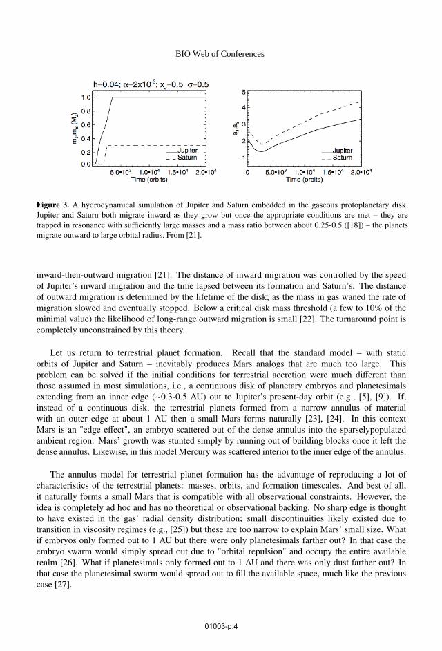
Figure 3. A hydrodynamical simulation of Jupiter and Saturn embedded in the gaseous protoplanetary disk. Jupiter and Saturn both migrate inward as they grow but once the appropriate conditions are met – they are trapped in resonance with sufficiently large masses and a mass ratio between about 0.25-0.5 ([18]) – the planets migrate outward to large orbital radius. From [21].

inward-then-outward migration [21]. The distance of inward migration was controlled by the speedof Jupiter’s inward migration and the time lapsed between its formation and Saturn’s. The distanceof outward migration is determined by the lifetime of the disk; as the mass in gas waned the rate ofmigration slowed and eventually stopped. Below a critical disk mass threshold (a few to 10% of theminimal value) the likelihood of long-range outward migration is small [22]. The turnaround point iscompletely unconstrained by this theory.

Let us return to terrestrial planet formation. Recall that the standard model – with staticorbits of Jupiter and Saturn – inevitably produces Mars analogs that are much too large. Thisproblem can be solved if the initial conditions for terrestrial accretion were much different thanthose assumed in most simulations, i.e., a continuous disk of planetary embryos and planetesimalsextending from an inner edge (∼0.3-0.5 AU) out to Jupiter’s present-day orbit (e.g., [5], [9]). If,instead of a continuous disk, the terrestrial planets formed from a narrow annulus of materialwith an outer edge at about 1 AU then a small Mars forms naturally [23], [24]. In this contextMars is an "edge effect", an embryo scattered out of the dense annulus into the sparselypopulatedambient region. Mars’ growth was stunted simply by running out of building blocks once it left thedense annulus. Likewise, in this model Mercury was scattered interior to the inner edge of the annulus.

The annulus model for terrestrial planet formation has the advantage of reproducing a lot ofcharacteristics of the terrestrial planets: masses, orbits, and formation timescales. And best of all,it naturally forms a small Mars that is compatible with all observational constraints. However, theidea is completely ad hoc and has no theoretical or observational backing. No sharp edge is thoughtto have existed in the gas’ radial density distribution; small discontinuities likely existed due totransition in viscosity regimes (e.g., [25]) but these are too narrow to explain Mars’ small size. Whatif embryos only formed out to 1 AU but there were only planetesimals farther out? In that case theembryo swarm would simply spread out due to "orbital repulsion" and occupy the entire availablerealm [26]. What if planetesimals only formed out to 1 AU and there was only dust farther out? Inthat case the planetesimal swarm would spread out to fill the available space, much like the previouscase [27].

BIO Web of Conferences

01003-p.4

What if Jupiter were at 1.5 AU? In that case, any embryos or planetesimals exterior to ∼1 AUwould be dynamically ejected very quickly and there would indeed be the sharp edge needed toreproduce Mars.

3 The "Grand Tack" model

In the context of the inward-then-outward migration of Jupiter and Saturn described above, there wasno constraint on the turnaround point, where Jupiter "tacked" (a sailing term for a change of directionagainst the wind) and started migrating outward. What if that turnaround point was at 1.5 AU? Thisidea represented the birth of the "Grand Tack" model.

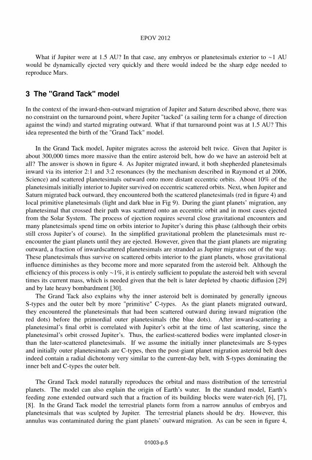
In the Grand Tack model, Jupiter migrates across the asteroid belt twice. Given that Jupiter isabout 300,000 times more massive than the entire asteroid belt, how do we have an asteroid belt atall? The answer is shown in figure 4. As Jupiter migrated inward, it both shepherded planetesimalsinward via its interior 2:1 and 3:2 resonances (by the mechanism described in Raymond et al 2006,Science) and scattered planetesimals outward onto more distant eccentric orbits. About 10% of theplanetesimals initially interior to Jupiter survived on eccentric scattered orbits. Next, when Jupiter andSaturn migrated back outward, they encountered both the scattered planetesimals (red in figure 4) andlocal primitive planetesimals (light and dark blue in Fig 9). During the giant planets’ migration, anyplanetesimal that crossed their path was scattered onto an eccentric orbit and in most cases ejectedfrom the Solar System. The process of ejection requires several close gravitational encounters andmany planetesimals spend time on orbits interior to Jupiter’s during this phase (although their orbitsstill cross Jupiter’s of course). In the simplified gravitational problem the planetesimals must re-encounter the giant planets until they are ejected. However, given that the giant planets are migratingoutward, a fraction of inwardscattered planetesimals are stranded as Jupiter migrates out of the way.These planetesimals thus survive on scattered orbits interior to the giant planets, whose gravitationalinfluence diminishes as they become more and more separated from the asteroid belt. Although theefficiency of this process is only ∼1%, it is entirely sufficient to populate the asteroid belt with severaltimes its current mass, which is needed given that the belt is later depleted by chaotic diffusion [29]and by late heavy bombardment [30].

The Grand Tack also explains why the inner asteroid belt is dominated by generally igneousS-types and the outer belt by more "primitive" C-types. As the giant planets migrated outward,they encountered the planetesimals that had been scattered outward during inward migration (thered dots) before the primordial outer planetesimals (the blue dots). After inward-scattering aplanetesimal’s final orbit is correlated with Jupiter’s orbit at the time of last scattering, since theplanetesimal’s orbit crossed Jupiter’s. Thus, the earliest-scattered bodies were implanted closer-inthan the later-scattered planetesimals. If we assume the initially inner planetesimals are S-typesand initially outer planetesimals are C-types, then the post-giant planet migration asteroid belt doesindeed contain a radial dichotomy very similar to the current-day belt, with S-types dominating theinner belt and C-types the outer belt.

The Grand Tack model naturally reproduces the orbital and mass distribution of the terrestrialplanets. The model can also explain the origin of Earth’s water. In the standard model, Earth’sfeeding zone extended outward such that a fraction of its building blocks were water-rich [6], [7],[8]. In the Grand Tack model the terrestrial planets form from a narrow annulus of embryos andplanetesimals that was sculpted by Jupiter. The terrestrial planets should be dry. However, thisannulus was contaminated during the giant planets’ outward migration. As can be seen in figure 4,

EPOV 2012

01003-p.5

Figure 4. A representative simulation of the Grand Tack model [28]. Here the black dots represent the giant planets. Jupiter and Saturn follow the evolution described in the text. The red dots are planetesimals that origi-nated interior to Jupiter’s orbit, the light blue dots planetesimals starting between the giant planets, and the dark blue dots more distant planetesimals. The open circles are terrestrial embryos. After the giant planets’ two-phase migration the whole inner Solar System is reproduced: the terrestrial planets’ masses and orbits and the mass, mass distribution and radial dichotomy of the asteroid belt.

many planetesimals that were scattered inward by Jupiter "overshot" the asteroid belt and ended upon orbits that entered the inner Solar System. Indeed, for every planetesimal that was trapped on astable orbit in the asteroid belt, 10-20 were scattered onto orbits with perihelion distances of 1-1.5AU. These scattered C-type bodies were sufficient in number to deliver the requisite amount of waterto Earth (see figure 5). Compared with the standard model, a factor a few less water is delivered toEarth, but still several times more than its current water budget [31]. And this water also matchesthe chemical constraints because it is also delivered by C-types, although in this context by the sameparent population that was implanted into the asteroid belt as Ctypes.

BIO Web of Conferences

01003-p.6

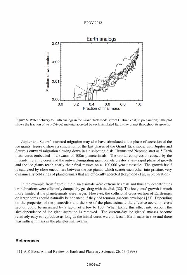
Figure 5. Water delivery to Earth analogs in the Grand Tack model (from O’Brien et al, in preparation). The plotshows the fraction of wet (C-type) material accreted by each simulated Earth-like planet throughout its growth.

Jupiter and Saturn’s outward migration may also have stimulated a late phase of accretion of theice giants. figure 6 shows a simulation of the last phases of the Grand Tack model with Jupiter andSaturn’s outward migration slowing down in a dissipating disk. Uranus and Neptune start as 5 Earthmass cores embedded in a swarm of 100m planetesimals. The orbital compression caused by theinward-migrating cores and the outward-migrating giant planets creates a very rapid phase of growthand the ice giants reach nearly their final masses on a 100,000 year timescale. The growth itselfis catalyzed by close encounters between the ice giants, which scatter each other into pristine, verydynamically cold rings of planetesimals that are efficiently accreted (Raymond et al, in preparation).

In the example from figure 6 the planetesimals were extremely small and thus any eccentricitiesor inclinations were efficiently damped by gas drag with the disk [32]. The ice giants’ growth is muchmore limited if the planetesimals were larger. However, the collisional cross-section of Earth-massor larger cores should naturally be enhanced if they had tenuous gaseous envelopes [33]. Dependingon the properties of the planet/disk and the size of the planetesimals, the effective accretion crosssection could be increased by a factor of a few to 100. When taking this effect into account thesize-dependence of ice giant accretion is removed. The current-day ice giants’ masses becomerelatively easy to reproduce as long as the initial cores were at least 1 Earth mass in size and therewas sufficient mass in the planetesimal swarm.

References

[1] A.P. Boss, Annual Review of Earth and Planetary Sciences 26, 53 (1998)

EPOV 2012

01003-p.7

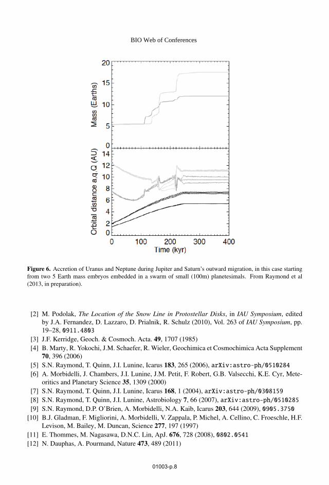
Figure 6. Accretion of Uranus and Neptune during Jupiter and Saturn’s outward migration, in this case startingfrom two 5 Earth mass embryos embedded in a swarm of small (100m) planetesimals. From Raymond et al(2013, in preparation).

[2] M. Podolak, The Location of the Snow Line in Protostellar Disks, in IAU Symposium, editedby J.A. Fernandez, D. Lazzaro, D. Prialnik, R. Schulz (2010), Vol. 263 of IAU Symposium, pp.19–28, 0911.4803

[3] J.F. Kerridge, Geoch. & Cosmoch. Acta. 49, 1707 (1985)[4] B. Marty, R. Yokochi, J.M. Schaefer, R. Wieler, Geochimica et Cosmochimica Acta Supplement

70, 396 (2006)[5] S.N. Raymond, T. Quinn, J.I. Lunine, Icarus 183, 265 (2006), arXiv:astro-ph/0510284[6] A. Morbidelli, J. Chambers, J.I. Lunine, J.M. Petit, F. Robert, G.B. Valsecchi, K.E. Cyr, Mete-

oritics and Planetary Science 35, 1309 (2000)[7] S.N. Raymond, T. Quinn, J.I. Lunine, Icarus 168, 1 (2004), arXiv:astro-ph/0308159[8] S.N. Raymond, T. Quinn, J.I. Lunine, Astrobiology 7, 66 (2007), arXiv:astro-ph/0510285[9] S.N. Raymond, D.P. O’Brien, A. Morbidelli, N.A. Kaib, Icarus 203, 644 (2009), 0905.3750

[10] B.J. Gladman, F. Migliorini, A. Morbidelli, V. Zappala, P. Michel, A. Cellino, C. Froeschle, H.F.Levison, M. Bailey, M. Duncan, Science 277, 197 (1997)

[11] E. Thommes, M. Nagasawa, D.N.C. Lin, ApJ. 676, 728 (2008), 0802.0541[12] N. Dauphas, A. Pourmand, Nature 473, 489 (2011)

BIO Web of Conferences

01003-p.8

[13] R. Malhotra, AJ 110, 420 (1995), arXiv:astro-ph/9504036[14] H.F. Levison, A. Morbidelli, C. Van Laerhoven, R. Gomes, K. Tsiganis, Icarus 196, 258 (2008),

0712.0553

[15] J.M. Hahn, R. Malhotra, AJ 117, 3041 (1999), arXiv:astro-ph/9902370[16] F.S. Masset, J.C.B. Papaloizou, ApJ 588, 494 (2003), arXiv:astro-ph/0301171[17] A. Pierens, R.P. Nelson, A&A 482, 333 (2008), 0802.2033[18] F. Masset, M. Snellgrove, MNRAS 320, L55 (2001), arXiv:astro-ph/0003421[19] A. Morbidelli, A. Crida, Icarus 191, 158 (2007)[20] A. Crida, F. Masset, A. Morbidelli, ApJ 705, L148 (2009), 0910.1004[21] A. Pierens, S.N. Raymond, A&A 533, A131 (2011), 1107.5656[22] G. D’Angelo, F. Marzari, ApJ 757, 50 (2012), 1207.2737[23] G.W. Wetherill, Accumulation of the terrestrial planets, in IAU Colloq. 52: Protostars and Plan-

ets, edited by T. Gehrels (1978), pp. 565–598[24] B.M.S. Hansen, ApJ 703, 1131 (2009), 0908.0743[25] L. Jin, W.D. Arnett, N. Sui, X. Wang, ApJ 674, L105 (2008)[26] E. Kokubo, S. Ida, Icarus 123, 180 (1996)[27] Z.M. Leinhardt, D.C. Richardson, G. Lufkin, J. Haseltine, MNRAS 396, 718 (2009),

0903.2354

[28] K.J. Walsh, A. Morbidelli, S.N. Raymond, D.P. O’Brien, A.M. Mandell, Nature 475, 206 (2011),1201.5177

[29] D.A. Minton, R. Malhotra, Icarus 207, 744 (2010), 0909.3875[30] A. Morbidelli, R. Brasser, R. Gomes, H.F. Levison, K. Tsiganis, AJ 140, 1391 (2010),

1009.1521

[31] B. Marty, Earth and Planetary Science Letters 313, 56 (2012)[32] I. Adachi, C. Hayashi, K. Nakazawa, Progress of Theoretical Physics 56, 1756 (1976)[33] S. Inaba, M. Ikoma, A&A 410, 711 (2003)

EPOV 2012

01003-p.9