Embed Size (px)
Citation preview
Forensic DNA analysis and multi-locus matchprobability in finite populations:
A fundamental difference between the Moran and
Wright-Fisher models
Yun S. SongDepartments of EECS and Statistics
UC Berkeley
DIMACSApril 27, 2009
0 / 37
Introduction Random Mating Graphical Framework Results Other Works
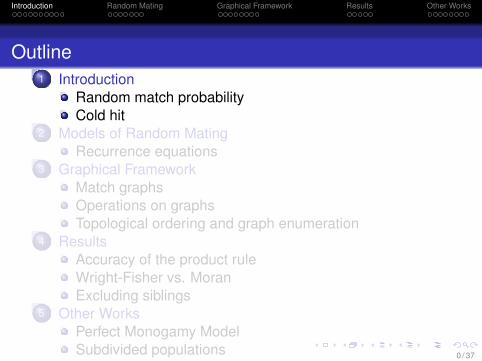
Outline1 Introduction
Random match probabilityCold hit
2 Models of Random MatingRecurrence equations
3 Graphical FrameworkMatch graphsOperations on graphsTopological ordering and graph enumeration
4 ResultsAccuracy of the product ruleWright-Fisher vs. MoranExcluding siblings
5 Other WorksPerfect Monogamy ModelSubdivided populationsFamilial search
0 / 37
Introduction Random Mating Graphical Framework Results Other Works
Random match probability
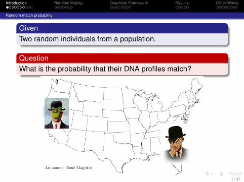
GivenTwo random individuals from a population.
QuestionWhat is the probability that their DNA profiles match?
Art source: Rene Magritte
1 / 37
Introduction Random Mating Graphical Framework Results Other Works
Random match probability
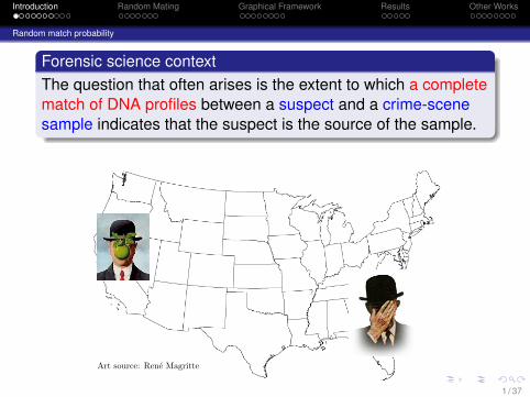
Forensic science contextThe question that often arises is the extent to which a completematch of DNA profiles between a suspect and a crime-scenesample indicates that the suspect is the source of the sample.
Art source: Rene Magritte
1 / 37
Introduction Random Mating Graphical Framework Results Other Works
Random match probability
Match probability depends on many factors, includingThe number of loci in the DNA profile.Mutation rates.Population history.
Art source: Rene Magritte
1 / 37
Introduction Random Mating Graphical Framework Results Other Works
Random match probability
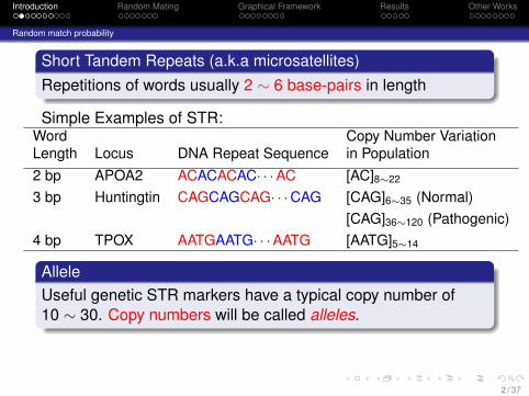
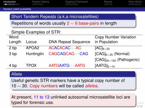
Short Tandem Repeats (a.k.a microsatellites)Repetitions of words usually 2 ∼ 6 base-pairs in length
Simple Examples of STR:Word Copy Number VariationLength Locus DNA Repeat Sequence in Population2 bp APOA2 ACACACAC· · ·AC [AC]8∼22
3 bp Huntingtin CAGCAGCAG· · ·CAG [CAG]6∼35 (Normal)[CAG]36∼120 (Pathogenic)
4 bp TPOX AATGAATG· · ·AATG [AATG]5∼14
AlleleUseful genetic STR markers have a typical copy number of10 ∼ 30. Copy numbers will be called alleles.
At present, 11 to 13 unlinked autosomal microsatellite loci aretyped for forensic use.
2 / 37
Introduction Random Mating Graphical Framework Results Other Works
Random match probability
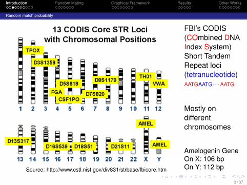
Source: http://www.cstl.nist.gov/div831/strbase/fbicore.htm
FBI’s CODIS(COmbined DNAIndex System)Short TandemRepeat loci(tetranucleotide)AATGAATG· · ·AATG
Mostly ondifferentchromosomes
Amelogenin GeneOn X: 106 bpOn Y: 112 bp
3 / 37
Introduction Random Mating Graphical Framework Results Other Works
Random match probability
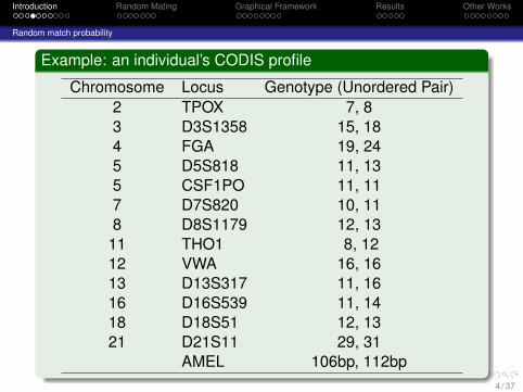
Example: an individual’s CODIS profile
Chromosome Locus Genotype (Unordered Pair)2 TPOX 7, 83 D3S1358 15, 184 FGA 19, 245 D5S818 11, 135 CSF1PO 11, 117 D7S820 10, 118 D8S1179 12, 1311 THO1 8, 1212 VWA 16, 1613 D13S317 11, 1616 D16S539 11, 1418 D18S51 12, 1321 D21S11 29, 31
AMEL 106bp, 112bp4 / 37
Introduction Random Mating Graphical Framework Results Other Works
Random match probability
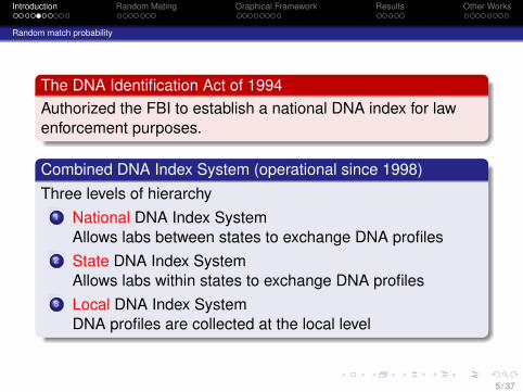
The DNA Identification Act of 1994Authorized the FBI to establish a national DNA index for lawenforcement purposes.
Combined DNA Index System (operational since 1998)Three levels of hierarchy
1 National DNA Index SystemAllows labs between states to exchange DNA profiles
2 State DNA Index SystemAllows labs within states to exchange DNA profiles
3 Local DNA Index SystemDNA profiles are collected at the local level
5 / 37
Introduction Random Mating Graphical Framework Results Other Works
Random match probability
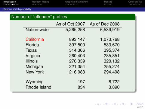
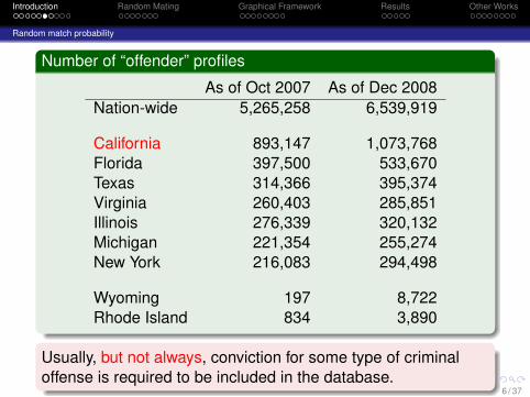
Number of “offender” profiles
As of Oct 2007 As of Dec 2008Nation-wide 5,265,258 6,539,919
California 893,147 1,073,768Florida 397,500 533,670Texas 314,366 395,374Virginia 260,403 285,851Illinois 276,339 320,132Michigan 221,354 255,274New York 216,083 294,498
Wyoming 197 8,722Rhode Island 834 3,890
Usually, but not always, conviction for some type of criminaloffense is required to be included in the database.
6 / 37
Introduction Random Mating Graphical Framework Results Other Works
Random match probability
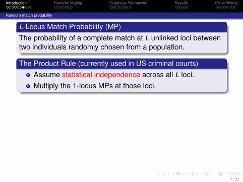
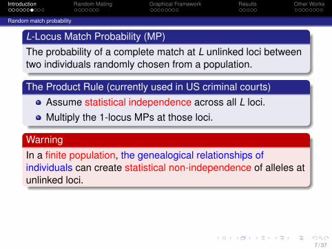
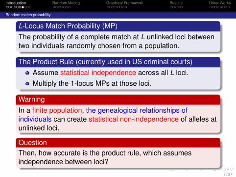
L-Locus Match Probability (MP)The probability of a complete match at L unlinked loci betweentwo individuals randomly chosen from a population.
The Product Rule (currently used in US criminal courts)Assume statistical independence across all L loci.Multiply the 1-locus MPs at those loci.
WarningIn a finite population, the genealogical relationships ofindividuals can create statistical non-independence of alleles atunlinked loci.
QuestionThen, how accurate is the product rule, which assumesindependence between loci?
7 / 37
Introduction Random Mating Graphical Framework Results Other Works
Random match probability
L-Locus Match Probability (MP)The probability of a complete match at L unlinked loci betweentwo individuals randomly chosen from a population.
The Product Rule (currently used in US criminal courts)Assume statistical independence across all L loci.Multiply the 1-locus MPs at those loci.
WarningIn a finite population, the genealogical relationships ofindividuals can create statistical non-independence of alleles atunlinked loci.
QuestionThen, how accurate is the product rule, which assumesindependence between loci?
7 / 37
Introduction Random Mating Graphical Framework Results Other Works
Cold hit
Question on QuestionIn any case, everyone believes that the true 13-locus MP is avery small number. Then, why are we interested in computing itaccurately?
Profile 1Profile 2Profile 3Profile 4Profile 5Profile 6
Profile d
Offender Database
Crime-scene sample
Unique match
8 / 37
Introduction Random Mating Graphical Framework Results Other Works
Cold hit
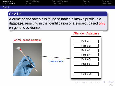
Cold HitA crime-scene sample is found to match a known profile in adatabase, resulting in the identification of a suspect based onlyon genetic evidence.
Profile 1Profile 2Profile 3Profile 4Profile 5Profile 6
Profile d
Offender Database
Crime-scene sample
Unique match
8 / 37
Introduction Random Mating Graphical Framework Results Other Works
Cold hit
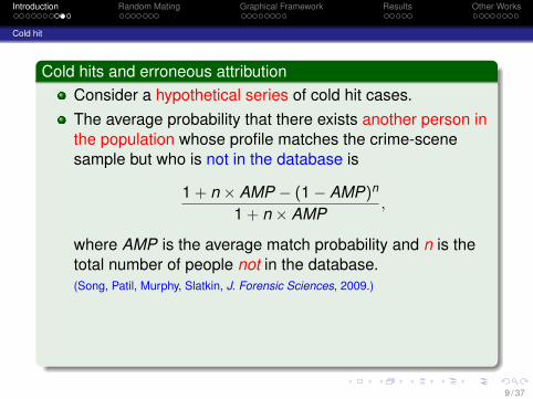
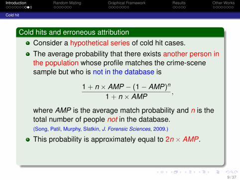
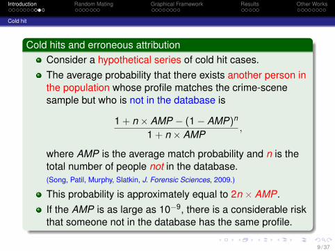
Cold hits and erroneous attributionConsider a hypothetical series of cold hit cases.
The average probability that there exists another person inthe population whose profile matches the crime-scenesample but who is not in the database is
1 + n × AMP − (1− AMP)n
1 + n × AMP,
where AMP is the average match probability and n is thetotal number of people not in the database.(Song, Patil, Murphy, Slatkin, J. Forensic Sciences, 2009.)
This probability is approximately equal to 2n × AMP.If the AMP is as large as 10−9, there is a considerable riskthat someone not in the database has the same profile.
9 / 37
Introduction Random Mating Graphical Framework Results Other Works
Cold hit
Cold hits and erroneous attributionConsider a hypothetical series of cold hit cases.The average probability that there exists another person inthe population whose profile matches the crime-scenesample but who is not in the database is
1 + n × AMP − (1− AMP)n
1 + n × AMP,
where AMP is the average match probability and n is thetotal number of people not in the database.(Song, Patil, Murphy, Slatkin, J. Forensic Sciences, 2009.)
This probability is approximately equal to 2n × AMP.
If the AMP is as large as 10−9, there is a considerable riskthat someone not in the database has the same profile.
9 / 37
Introduction Random Mating Graphical Framework Results Other Works
Cold hit
Cold hits and erroneous attributionConsider a hypothetical series of cold hit cases.The average probability that there exists another person inthe population whose profile matches the crime-scenesample but who is not in the database is
1 + n × AMP − (1− AMP)n
1 + n × AMP,
where AMP is the average match probability and n is thetotal number of people not in the database.(Song, Patil, Murphy, Slatkin, J. Forensic Sciences, 2009.)
This probability is approximately equal to 2n × AMP.If the AMP is as large as 10−9, there is a considerable riskthat someone not in the database has the same profile.
9 / 37
Introduction Random Mating Graphical Framework Results Other Works
Cold hit
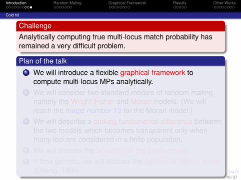
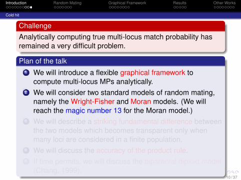
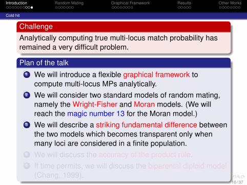
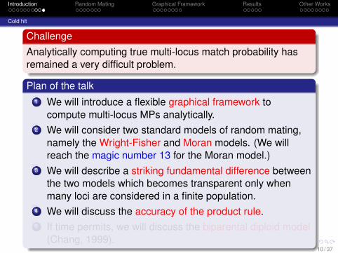
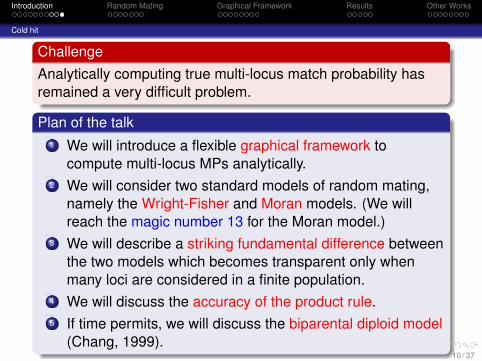
ChallengeAnalytically computing true multi-locus match probability hasremained a very difficult problem.
Plan of the talk1 We will introduce a flexible graphical framework to
compute multi-locus MPs analytically.2 We will consider two standard models of random mating,
namely the Wright-Fisher and Moran models. (We willreach the magic number 13 for the Moran model.)
3 We will describe a striking fundamental difference betweenthe two models which becomes transparent only whenmany loci are considered in a finite population.
4 We will discuss the accuracy of the product rule.5 If time permits, we will discuss the biparental diploid model
(Chang, 1999).10 / 37
Introduction Random Mating Graphical Framework Results Other Works
Cold hit
ChallengeAnalytically computing true multi-locus match probability hasremained a very difficult problem.
Plan of the talk1 We will introduce a flexible graphical framework to
compute multi-locus MPs analytically.2 We will consider two standard models of random mating,
namely the Wright-Fisher and Moran models. (We willreach the magic number 13 for the Moran model.)
3 We will describe a striking fundamental difference betweenthe two models which becomes transparent only whenmany loci are considered in a finite population.
4 We will discuss the accuracy of the product rule.5 If time permits, we will discuss the biparental diploid model
(Chang, 1999).10 / 37
Introduction Random Mating Graphical Framework Results Other Works
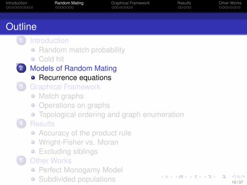
Outline1 Introduction
Random match probabilityCold hit
2 Models of Random MatingRecurrence equations
3 Graphical FrameworkMatch graphsOperations on graphsTopological ordering and graph enumeration
4 ResultsAccuracy of the product ruleWright-Fisher vs. MoranExcluding siblings
5 Other WorksPerfect Monogamy ModelSubdivided populationsFamilial search
10 / 37
Introduction Random Mating Graphical Framework Results Other Works
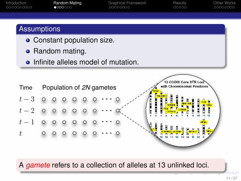
AssumptionsConstant population size.Random mating.Infinite alleles model of mutation.
Population of 2N gametes
t! 3t! 2t! 1t
Time
A gamete refers to a collection of alleles at 13 unlinked loci.
11 / 37
Introduction Random Mating Graphical Framework Results Other Works
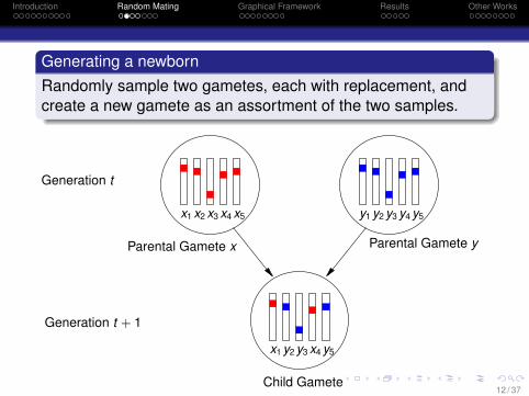
Generating a newbornRandomly sample two gametes, each with replacement, andcreate a new gamete as an assortment of the two samples.
Parental Gamete x
x1 y3 x4 y5y2
Generation t + 1
Child Gamete
x1 x3 x4 x5x2 y1 y3 y4 y5
Parental Gamete y
y2
Generation t
12 / 37
Introduction Random Mating Graphical Framework Results Other Works
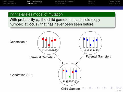
Infinite-alleles model of mutationWith probability µi , the child gamete has an allele (copynumber) at locus i that has never been seen before.
Child Gamete
x1 x3 x4 x5x2 y1 y3 y4 y5
Parental Gamete y
y2
Generation t
Parental Gamete x
x1 z3 x4 y5y2
Generation t + 1
12 / 37
Introduction Random Mating Graphical Framework Results Other Works
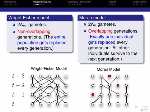
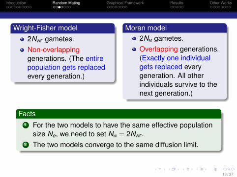
Wright-Fisher model2NWF gametes.Non-overlappinggenerations. (The entirepopulation gets replacedevery generation.)
Moran model2NM gametes.Overlapping generations.(Exactly one individualgets replaced everygeneration. All otherindividuals survive to thenext generation.)
t! 3t! 2t! 1t
Wright-Fisher Model Moran Model
13 / 37
Introduction Random Mating Graphical Framework Results Other Works
Wright-Fisher model2NWF gametes.Non-overlappinggenerations. (The entirepopulation gets replacedevery generation.)
Moran model2NM gametes.Overlapping generations.(Exactly one individualgets replaced everygeneration. All otherindividuals survive to thenext generation.)
Facts1 For the two models to have the same effective population
size Ne, we need to set NM = 2NWF.2 The two models converge to the same diffusion limit.
13 / 37
Introduction Random Mating Graphical Framework Results Other Works
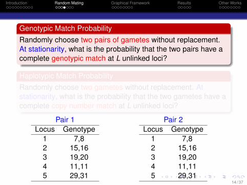
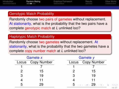
Genotypic Match ProbabilityRandomly choose two pairs of gametes without replacement.At stationarity, what is the probability that the two pairs have acomplete genotypic match at L unlinked loci?
Haplotypic Match ProbabilityRandomly choose two gametes without replacement. Atstationarity, what is the probability that the two gametes have acomplete copy number match at L unlinked loci?
Pair 1Locus Genotype
1 7,82 15,163 19,204 11,115 29,31
Pair 2Locus Genotype
1 7,82 15,163 19,204 11,115 29,31
14 / 37
Introduction Random Mating Graphical Framework Results Other Works
Genotypic Match ProbabilityRandomly choose two pairs of gametes without replacement.At stationarity, what is the probability that the two pairs have acomplete genotypic match at L unlinked loci?
Haplotypic Match ProbabilityRandomly choose two gametes without replacement. Atstationarity, what is the probability that the two gametes have acomplete copy number match at L unlinked loci?
Gamete xLocus Copy Number
1 72 153 194 115 29
Gamete yLocus Copy Number
1 72 153 194 115 29
14 / 37
Introduction Random Mating Graphical Framework Results Other Works
Recurrence equations
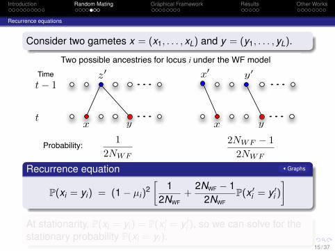
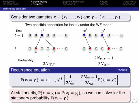
Consider two gametes x = (x1, . . . , xL) and y = (y1, . . . , yL).
t! 1
t
Time
x y
x! y!z!
x y
Two possible ancestries for locus i under the WF model
12NWF
2NWF ! 12NWF
Probability:
Recurrence equation Graphs
P(xi = yi) = (1− µi)2[
12NWF
+2NWF − 1
2NWFP(x ′
i = y ′i )
]At stationarity, P(xi = yi) = P(x ′
i = y ′i ), so we can solve for the
stationary probability P(xi = yi).15 / 37
Introduction Random Mating Graphical Framework Results Other Works
Recurrence equations
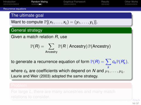
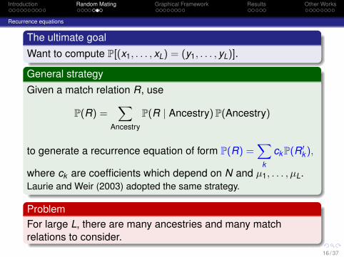
The ultimate goal
Want to compute P[(x1, . . . , xL) = (y1, . . . , yL)].
General strategy
Given a match relation R, use
P(R) =∑
Ancestry
P(R | Ancestry) P(Ancestry)
to generate a recurrence equation of form P(R) =∑
k
ckP(R′k ),
where ck are coefficients which depend on N and µ1, . . . , µL.Laurie and Weir (2003) adopted the same strategy.
ProblemFor large L, there are many ancestries and many matchrelations to consider.
16 / 37
Introduction Random Mating Graphical Framework Results Other Works
Recurrence equations
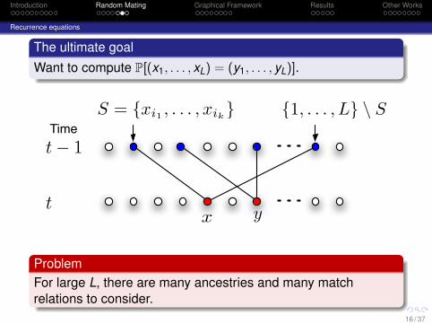
The ultimate goal
Want to compute P[(x1, . . . , xL) = (y1, . . . , yL)].
t! 1
t
Time
x
S = {xi1 , . . . , xik} {1, . . . , L} \ S
y
ProblemFor large L, there are many ancestries and many matchrelations to consider.
16 / 37
Introduction Random Mating Graphical Framework Results Other Works
Recurrence equations
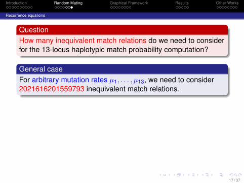
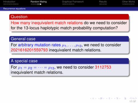
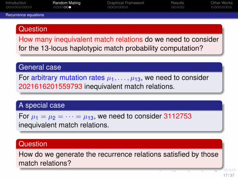
QuestionHow many inequivalent match relations do we need to considerfor the 13-locus haplotypic match probability computation?
General caseFor arbitrary mutation rates µ1, . . . , µ13, we need to consider2021616201559793 inequivalent match relations.
A special caseFor µ1 = µ2 = · · · = µ13, we need to consider 3112753inequivalent match relations.
QuestionHow do we generate the recurrence relations satisfied by thosematch relations?
17 / 37
Introduction Random Mating Graphical Framework Results Other Works
Recurrence equations
QuestionHow many inequivalent match relations do we need to considerfor the 13-locus haplotypic match probability computation?
General caseFor arbitrary mutation rates µ1, . . . , µ13, we need to consider2021616201559793 inequivalent match relations.
A special caseFor µ1 = µ2 = · · · = µ13, we need to consider 3112753inequivalent match relations.
QuestionHow do we generate the recurrence relations satisfied by thosematch relations?
17 / 37
Introduction Random Mating Graphical Framework Results Other Works
Outline1 Introduction
Random match probabilityCold hit
2 Models of Random MatingRecurrence equations
3 Graphical FrameworkMatch graphsOperations on graphsTopological ordering and graph enumeration
4 ResultsAccuracy of the product ruleWright-Fisher vs. MoranExcluding siblings
5 Other WorksPerfect Monogamy ModelSubdivided populationsFamilial search
17 / 37
Introduction Random Mating Graphical Framework Results Other Works
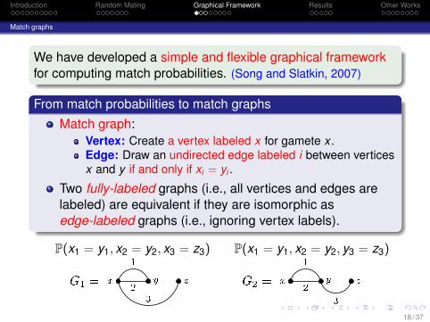
Match graphs
We have developed a simple and flexible graphical frameworkfor computing match probabilities. (Song and Slatkin, 2007)
From match probabilities to match graphsMatch graph:
Vertex: Create a vertex labeled x for gamete x .Edge: Draw an undirected edge labeled i between verticesx and y if and only if xi = yi .
Two fully-labeled graphs (i.e., all vertices and edges arelabeled) are equivalent if they are isomorphic asedge-labeled graphs (i.e., ignoring vertex labels).
P(x1 = y1, x2 = y2, x3 = z3) P(x1 = y1, x2 = y2, y3 = z3)G1 = x y z12 3 G2 = x y z12 318 / 37
Introduction Random Mating Graphical Framework Results Other Works
Match graphs
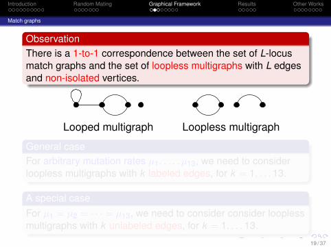
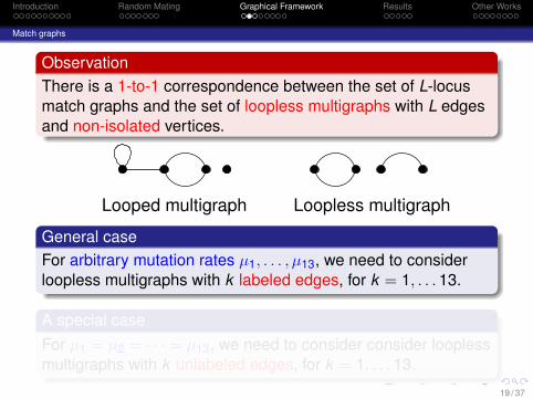
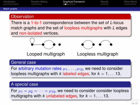
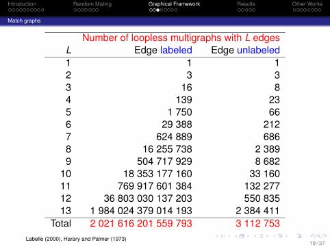
ObservationThere is a 1-to-1 correspondence between the set of L-locusmatch graphs and the set of loopless multigraphs with L edgesand non-isolated vertices.
Looped multigraph Loopless multigraph
General caseFor arbitrary mutation rates µ1, . . . , µ13, we need to considerloopless multigraphs with k labeled edges, for k = 1, . . . 13.
A special caseFor µ1 = µ2 = · · · = µ13, we need to consider consider looplessmultigraphs with k unlabeled edges, for k = 1, . . . 13.
19 / 37
Introduction Random Mating Graphical Framework Results Other Works
Match graphs
Number of loopless multigraphs with L edgesL Edge labeled Edge unlabeled1 1 12 3 33 16 84 139 235 1 750 666 29 388 2127 624 889 6868 16 255 738 2 3899 504 717 929 8 682
10 18 353 177 160 33 16011 769 917 601 384 132 27712 36 803 030 137 203 550 83513 1 984 024 379 014 193 2 384 411
Total 2 021 616 201 559 793 3 112 753Labelle (2000), Harary and Palmer (1973)
19 / 37
Introduction Random Mating Graphical Framework Results Other Works
Operations on graphs
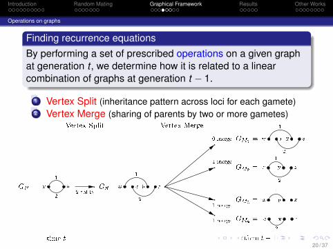
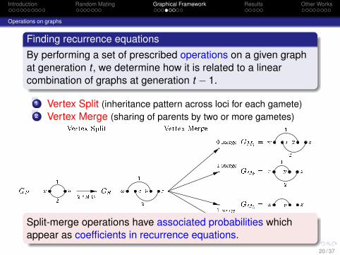
Finding recurrence equationsBy performing a set of prescribed operations on a given graphat generation t , we determine how it is related to a linearcombination of graphs at generation t − 1.
1 Vertex Split (inheritance pattern across loci for each gamete)2 Vertex Merge (sharing of parents by two or more gametes)
GP = x y12 GS =w x y z1 2w x y z1 2x y z1 2x y z1x y z2
GM1 =GM2 =GM3 =GM4 =2 splits0 merge1 merge1 merge1 merge
Vertex Split Vertex Merge
time t time t� 1
Split-merge operations have associated probabilities whichappear as coefficients in recurrence equations.
20 / 37
Introduction Random Mating Graphical Framework Results Other Works
Operations on graphs
Finding recurrence equationsBy performing a set of prescribed operations on a given graphat generation t , we determine how it is related to a linearcombination of graphs at generation t − 1.
1 Vertex Split (inheritance pattern across loci for each gamete)2 Vertex Merge (sharing of parents by two or more gametes)
GP = x y12 GS =w x y z1 2w x y z1 2x y z1 2x y z1x y z2
GM1 =GM2 =GM3 =GM4 =2 splits0 merge1 merge1 merge1 merge
Vertex Split Vertex Merge
time t time t� 1Split-merge operations have associated probabilities whichappear as coefficients in recurrence equations.
20 / 37
Introduction Random Mating Graphical Framework Results Other Works
Operations on graphs
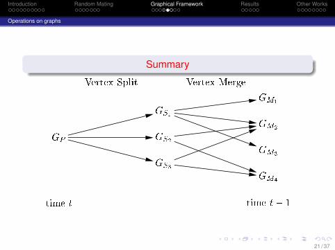
Summary
GP GS1GS2GS3GM1GM2GM3GM4
Vertex Split Vertex Mergetime t time t� 1
21 / 37
Introduction Random Mating Graphical Framework Results Other Works
Operations on graphs
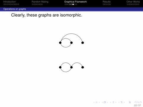
Clearly, these graphs are isomorphic.
22 / 37
Introduction Random Mating Graphical Framework Results Other Works
Operations on graphs
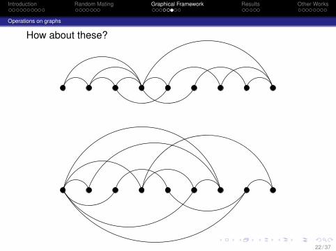
How about these?
22 / 37
Introduction Random Mating Graphical Framework Results Other Works
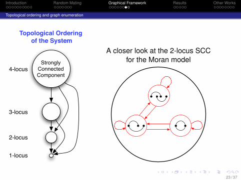
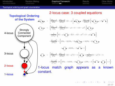
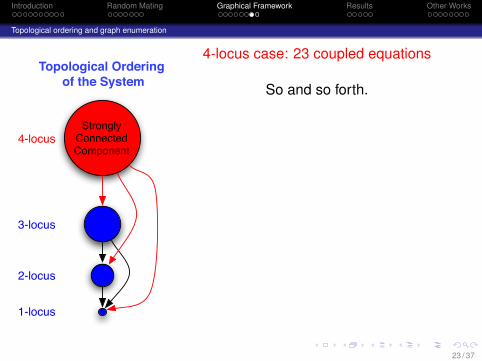
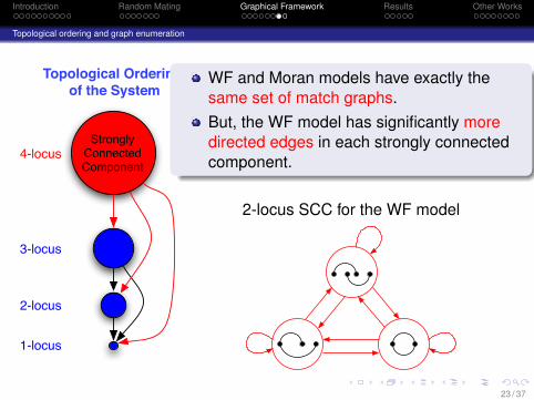
Topological ordering and graph enumeration
1-locus
2-locus
3-locus
4-locus
Topological Ordering of the System
StronglyConnectedComponent
A closer look at the 2-locus SCCfor the Moran model
23 / 37
Introduction Random Mating Graphical Framework Results Other Works
Topological ordering and graph enumeration
1-locus
2-locus
3-locus
4-locus
Topological Ordering of the System
StronglyConnectedComponent
1-locus case: 1 equation
Wright-Fisher model:
= (1− µ)2"
2NWF − 1
2NWF
+1
2NWF
#
Ancestry
Moran model:=
"
2NM − 2
2NM
+2NM − 1
(2NM)22(1−µ)
#
+2(1− µ)
(2NM)2
23 / 37
Introduction Random Mating Graphical Framework Results Other Works
Topological ordering and graph enumeration
1-locus
2-locus
3-locus
4-locus
Topological Ordering of the System
StronglyConnectedComponent
2-locus case: 3 coupled equations
=
"
2NM − 4
2NM
+2NM − 3
(2NM)2· 4(1 − µ)
#
+2(1 − µ)
(2NM)2
4 + 2
!
=
(
2NM − 3
2NM
+2NM − 2
(2NM)2[2(1 − µ) + (1 − r)(1 − µ)2]
)
+1
(2NM)2
(
2(1 − µ) + 2[(1 − r)(1 − µ)2 + (1 − µ)]
)
+(1 − µ)2
(2NM)3· r
(
(2NM − 2)(2NM − 3) + 3(2NM − 2)
+ + 2(2NM − 1) + 1
)
=
"
2NM − 2
2NM
+2NM − 1
(2NM)2· 2(1 − µ)2(1 − r)
#
+1
(2NM)22(1 − µ)2(1 − r)
+(1 − µ)2
(2NM)3· 2r
(
(2NM − 1)(2NM − 2) + (2NM − 1)
"
2 +
#
+ 1
)
1-locus match graph appears as a knownconstant.
23 / 37
Introduction Random Mating Graphical Framework Results Other Works
Topological ordering and graph enumeration
1-locus
2-locus
3-locus
4-locus
Topological Ordering of the System
StronglyConnectedComponent
3-locus case: 8 coupled equations
1-locus and 2-locus match graphs are treated asknown constants.
23 / 37
Introduction Random Mating Graphical Framework Results Other Works
Topological ordering and graph enumeration
1-locus
2-locus
3-locus
4-locus
Topological Ordering of the System
StronglyConnectedComponent
4-locus case: 23 coupled equations
So and so forth.
23 / 37
Introduction Random Mating Graphical Framework Results Other Works
Topological ordering and graph enumeration
1-locus
2-locus
3-locus
4-locus
Topological Ordering of the System
StronglyConnectedComponent
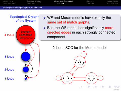
WF and Moran models have exactly thesame set of match graphs.But, the WF model has significantly moredirected edges in each strongly connectedcomponent.
2-locus SCC for the WF model
23 / 37
Introduction Random Mating Graphical Framework Results Other Works
Topological ordering and graph enumeration
1-locus
2-locus
3-locus
4-locus
Topological Ordering of the System
StronglyConnectedComponent
WF and Moran models have exactly thesame set of match graphs.But, the WF model has significantly moredirected edges in each strongly connectedcomponent.
2-locus SCC for the Moran model
23 / 37
Introduction Random Mating Graphical Framework Results Other Works
Topological ordering and graph enumeration
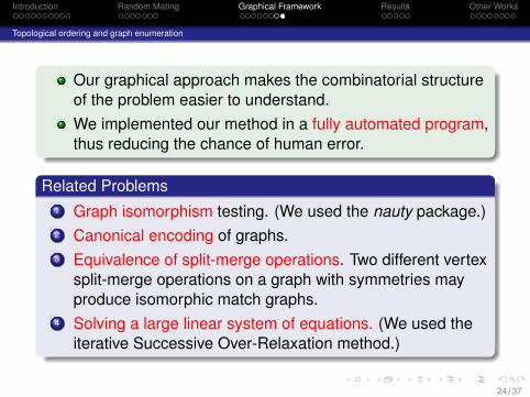
Our graphical approach makes the combinatorial structureof the problem easier to understand.We implemented our method in a fully automated program,thus reducing the chance of human error.
Related Problems1 Graph isomorphism testing. (We used the nauty package.)2 Canonical encoding of graphs.3 Equivalence of split-merge operations. Two different vertex
split-merge operations on a graph with symmetries mayproduce isomorphic match graphs.
4 Solving a large linear system of equations. (We used theiterative Successive Over-Relaxation method.)
24 / 37
Introduction Random Mating Graphical Framework Results Other Works
Outline1 Introduction
Random match probabilityCold hit
2 Models of Random MatingRecurrence equations
3 Graphical FrameworkMatch graphsOperations on graphsTopological ordering and graph enumeration
4 ResultsAccuracy of the product ruleWright-Fisher vs. MoranExcluding siblings
5 Other WorksPerfect Monogamy ModelSubdivided populationsFamilial search
24 / 37
Introduction Random Mating Graphical Framework Results Other Works
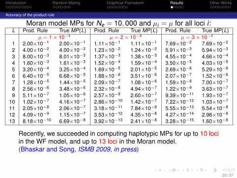
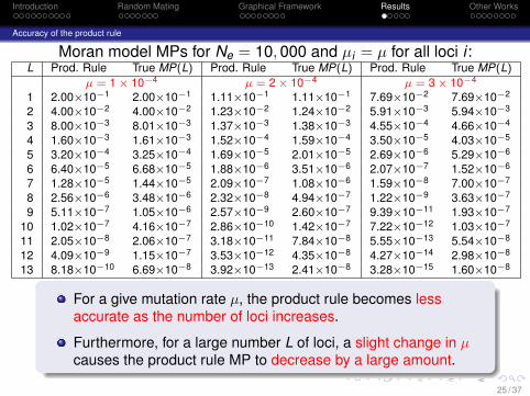
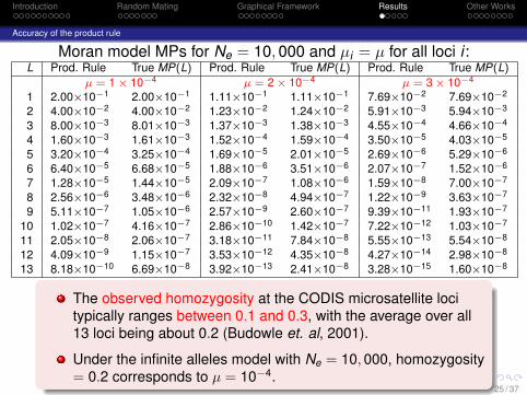
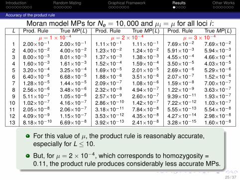
Accuracy of the product rule
Moran model MPs for Ne = 10, 000 and µi = µ for all loci i :L Prod. Rule True MP(L) Prod. Rule True MP(L) Prod. Rule True MP(L)
µ = 1 × 10⁻⁴ µ = 2 × 10⁻⁴ µ = 3 × 10⁻⁴
1 2.00×10⁻¹ 2.00×10⁻¹ 1.11×10⁻¹ 1.11×10⁻¹ 7.69×10⁻² 7.69×10⁻²
2 4.00×10⁻² 4.00×10⁻² 1.23×10⁻² 1.24×10⁻² 5.91×10⁻³ 5.94×10⁻³
3 8.00×10⁻³ 8.01×10⁻³ 1.37×10⁻³ 1.38×10⁻³ 4.55×10⁻⁴ 4.66×10⁻⁴
4 1.60×10⁻³ 1.61×10⁻³ 1.52×10⁻⁴ 1.59×10⁻⁴ 3.50×10⁻⁵ 4.03×10⁻⁵
5 3.20×10⁻⁴ 3.25×10⁻⁴ 1.69×10⁻⁵ 2.01×10⁻⁵ 2.69×10⁻⁶ 5.29×10⁻⁶
6 6.40×10⁻⁵ 6.68×10⁻⁵ 1.88×10⁻⁶ 3.51×10⁻⁶ 2.07×10⁻⁷ 1.52×10⁻⁶
7 1.28×10⁻⁵ 1.44×10⁻⁵ 2.09×10⁻⁷ 1.08×10⁻⁶ 1.59×10⁻⁸ 7.00×10⁻⁷
8 2.56×10⁻⁶ 3.48×10⁻⁶ 2.32×10⁻⁸ 4.94×10⁻⁷ 1.22×10⁻⁹ 3.63×10⁻⁷
9 5.11×10⁻⁷ 1.05×10⁻⁶ 2.57×10⁻⁹ 2.60×10⁻⁷ 9.39×10⁻¹¹ 1.93×10⁻⁷
10 1.02×10⁻⁷ 4.16×10⁻⁷ 2.86×10⁻¹⁰ 1.42×10⁻⁷ 7.22×10⁻¹² 1.03×10⁻⁷
11 2.05×10⁻⁸ 2.06×10⁻⁷ 3.18×10⁻¹¹ 7.84×10⁻⁸ 5.55×10⁻¹³ 5.54×10⁻⁸
12 4.09×10⁻⁹ 1.15×10⁻⁷ 3.53×10⁻¹² 4.35×10⁻⁸ 4.27×10⁻¹⁴ 2.98×10⁻⁸
13 8.18×10⁻¹⁰ 6.69×10⁻⁸ 3.92×10⁻¹³ 2.41×10⁻⁸ 3.28×10⁻¹⁵ 1.60×10⁻⁸
Recently, we succeeded in computing haplotypic MPs for up to 10 lociin the WF model, and up to 13 loci in the Moran model.(Bhaskar and Song, ISMB 2009, in press)
25 / 37
Introduction Random Mating Graphical Framework Results Other Works
Accuracy of the product rule
Moran model MPs for Ne = 10, 000 and µi = µ for all loci i :L Prod. Rule True MP(L) Prod. Rule True MP(L) Prod. Rule True MP(L)
µ = 1 × 10⁻⁴ µ = 2 × 10⁻⁴ µ = 3 × 10⁻⁴
1 2.00×10⁻¹ 2.00×10⁻¹ 1.11×10⁻¹ 1.11×10⁻¹ 7.69×10⁻² 7.69×10⁻²
2 4.00×10⁻² 4.00×10⁻² 1.23×10⁻² 1.24×10⁻² 5.91×10⁻³ 5.94×10⁻³
3 8.00×10⁻³ 8.01×10⁻³ 1.37×10⁻³ 1.38×10⁻³ 4.55×10⁻⁴ 4.66×10⁻⁴
4 1.60×10⁻³ 1.61×10⁻³ 1.52×10⁻⁴ 1.59×10⁻⁴ 3.50×10⁻⁵ 4.03×10⁻⁵
5 3.20×10⁻⁴ 3.25×10⁻⁴ 1.69×10⁻⁵ 2.01×10⁻⁵ 2.69×10⁻⁶ 5.29×10⁻⁶
6 6.40×10⁻⁵ 6.68×10⁻⁵ 1.88×10⁻⁶ 3.51×10⁻⁶ 2.07×10⁻⁷ 1.52×10⁻⁶
7 1.28×10⁻⁵ 1.44×10⁻⁵ 2.09×10⁻⁷ 1.08×10⁻⁶ 1.59×10⁻⁸ 7.00×10⁻⁷
8 2.56×10⁻⁶ 3.48×10⁻⁶ 2.32×10⁻⁸ 4.94×10⁻⁷ 1.22×10⁻⁹ 3.63×10⁻⁷
9 5.11×10⁻⁷ 1.05×10⁻⁶ 2.57×10⁻⁹ 2.60×10⁻⁷ 9.39×10⁻¹¹ 1.93×10⁻⁷
10 1.02×10⁻⁷ 4.16×10⁻⁷ 2.86×10⁻¹⁰ 1.42×10⁻⁷ 7.22×10⁻¹² 1.03×10⁻⁷
11 2.05×10⁻⁸ 2.06×10⁻⁷ 3.18×10⁻¹¹ 7.84×10⁻⁸ 5.55×10⁻¹³ 5.54×10⁻⁸
12 4.09×10⁻⁹ 1.15×10⁻⁷ 3.53×10⁻¹² 4.35×10⁻⁸ 4.27×10⁻¹⁴ 2.98×10⁻⁸
13 8.18×10⁻¹⁰ 6.69×10⁻⁸ 3.92×10⁻¹³ 2.41×10⁻⁸ 3.28×10⁻¹⁵ 1.60×10⁻⁸
For a give mutation rate µ, the product rule becomes lessaccurate as the number of loci increases.
Furthermore, for a large number L of loci, a slight change in µcauses the product rule MP to decrease by a large amount.
25 / 37
Introduction Random Mating Graphical Framework Results Other Works
Accuracy of the product rule
Moran model MPs for Ne = 10, 000 and µi = µ for all loci i :L Prod. Rule True MP(L) Prod. Rule True MP(L) Prod. Rule True MP(L)
µ = 1 × 10⁻⁴ µ = 2 × 10⁻⁴ µ = 3 × 10⁻⁴
1 2.00×10⁻¹ 2.00×10⁻¹ 1.11×10⁻¹ 1.11×10⁻¹ 7.69×10⁻² 7.69×10⁻²
2 4.00×10⁻² 4.00×10⁻² 1.23×10⁻² 1.24×10⁻² 5.91×10⁻³ 5.94×10⁻³
3 8.00×10⁻³ 8.01×10⁻³ 1.37×10⁻³ 1.38×10⁻³ 4.55×10⁻⁴ 4.66×10⁻⁴
4 1.60×10⁻³ 1.61×10⁻³ 1.52×10⁻⁴ 1.59×10⁻⁴ 3.50×10⁻⁵ 4.03×10⁻⁵
5 3.20×10⁻⁴ 3.25×10⁻⁴ 1.69×10⁻⁵ 2.01×10⁻⁵ 2.69×10⁻⁶ 5.29×10⁻⁶
6 6.40×10⁻⁵ 6.68×10⁻⁵ 1.88×10⁻⁶ 3.51×10⁻⁶ 2.07×10⁻⁷ 1.52×10⁻⁶
7 1.28×10⁻⁵ 1.44×10⁻⁵ 2.09×10⁻⁷ 1.08×10⁻⁶ 1.59×10⁻⁸ 7.00×10⁻⁷
8 2.56×10⁻⁶ 3.48×10⁻⁶ 2.32×10⁻⁸ 4.94×10⁻⁷ 1.22×10⁻⁹ 3.63×10⁻⁷
9 5.11×10⁻⁷ 1.05×10⁻⁶ 2.57×10⁻⁹ 2.60×10⁻⁷ 9.39×10⁻¹¹ 1.93×10⁻⁷
10 1.02×10⁻⁷ 4.16×10⁻⁷ 2.86×10⁻¹⁰ 1.42×10⁻⁷ 7.22×10⁻¹² 1.03×10⁻⁷
11 2.05×10⁻⁸ 2.06×10⁻⁷ 3.18×10⁻¹¹ 7.84×10⁻⁸ 5.55×10⁻¹³ 5.54×10⁻⁸
12 4.09×10⁻⁹ 1.15×10⁻⁷ 3.53×10⁻¹² 4.35×10⁻⁸ 4.27×10⁻¹⁴ 2.98×10⁻⁸
13 8.18×10⁻¹⁰ 6.69×10⁻⁸ 3.92×10⁻¹³ 2.41×10⁻⁸ 3.28×10⁻¹⁵ 1.60×10⁻⁸
The observed homozygosity at the CODIS microsatellite locitypically ranges between 0.1 and 0.3, with the average over all13 loci being about 0.2 (Budowle et. al, 2001).
Under the infinite alleles model with Ne = 10, 000, homozygosity= 0.2 corresponds to µ = 10−4.
25 / 37
Introduction Random Mating Graphical Framework Results Other Works
Accuracy of the product rule
Moran model MPs for Ne = 10, 000 and µi = µ for all loci i :L Prod. Rule True MP(L) Prod. Rule True MP(L) Prod. Rule True MP(L)
µ = 1 × 10⁻⁴ µ = 2 × 10⁻⁴ µ = 3 × 10⁻⁴
1 2.00×10⁻¹ 2.00×10⁻¹ 1.11×10⁻¹ 1.11×10⁻¹ 7.69×10⁻² 7.69×10⁻²
2 4.00×10⁻² 4.00×10⁻² 1.23×10⁻² 1.24×10⁻² 5.91×10⁻³ 5.94×10⁻³
3 8.00×10⁻³ 8.01×10⁻³ 1.37×10⁻³ 1.38×10⁻³ 4.55×10⁻⁴ 4.66×10⁻⁴
4 1.60×10⁻³ 1.61×10⁻³ 1.52×10⁻⁴ 1.59×10⁻⁴ 3.50×10⁻⁵ 4.03×10⁻⁵
5 3.20×10⁻⁴ 3.25×10⁻⁴ 1.69×10⁻⁵ 2.01×10⁻⁵ 2.69×10⁻⁶ 5.29×10⁻⁶
6 6.40×10⁻⁵ 6.68×10⁻⁵ 1.88×10⁻⁶ 3.51×10⁻⁶ 2.07×10⁻⁷ 1.52×10⁻⁶
7 1.28×10⁻⁵ 1.44×10⁻⁵ 2.09×10⁻⁷ 1.08×10⁻⁶ 1.59×10⁻⁸ 7.00×10⁻⁷
8 2.56×10⁻⁶ 3.48×10⁻⁶ 2.32×10⁻⁸ 4.94×10⁻⁷ 1.22×10⁻⁹ 3.63×10⁻⁷
9 5.11×10⁻⁷ 1.05×10⁻⁶ 2.57×10⁻⁹ 2.60×10⁻⁷ 9.39×10⁻¹¹ 1.93×10⁻⁷
10 1.02×10⁻⁷ 4.16×10⁻⁷ 2.86×10⁻¹⁰ 1.42×10⁻⁷ 7.22×10⁻¹² 1.03×10⁻⁷
11 2.05×10⁻⁸ 2.06×10⁻⁷ 3.18×10⁻¹¹ 7.84×10⁻⁸ 5.55×10⁻¹³ 5.54×10⁻⁸
12 4.09×10⁻⁹ 1.15×10⁻⁷ 3.53×10⁻¹² 4.35×10⁻⁸ 4.27×10⁻¹⁴ 2.98×10⁻⁸
13 8.18×10⁻¹⁰ 6.69×10⁻⁸ 3.92×10⁻¹³ 2.41×10⁻⁸ 3.28×10⁻¹⁵ 1.60×10⁻⁸
For this value of µ, the product rule is reasonably accurate,especially for L ≤ 10.
But, for µ = 2× 10⁻⁴, which corresponds to homozygosity =0.11, the product rule produces considerably less accurate MPs.
25 / 37
Introduction Random Mating Graphical Framework Results Other Works
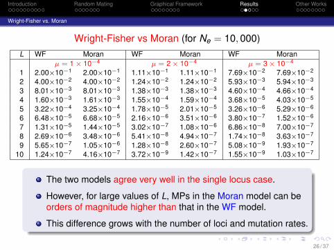
Wright-Fisher vs. Moran
Wright-Fisher vs Moran (for Ne = 10, 000)L WF Moran WF Moran WF Moran
µ = 1 × 10⁻⁴ µ = 2 × 10⁻⁴ µ = 3 × 10⁻⁴
1 2.00×10⁻¹ 2.00×10⁻¹ 1.11×10⁻¹ 1.11×10⁻¹ 7.69×10⁻² 7.69×10⁻²
2 4.00×10⁻² 4.00×10⁻² 1.24×10⁻² 1.24×10⁻² 5.93×10⁻³ 5.94×10⁻³
3 8.01×10⁻³ 8.01×10⁻³ 1.38×10⁻³ 1.38×10⁻³ 4.60×10⁻⁴ 4.66×10⁻⁴
4 1.60×10⁻³ 1.61×10⁻³ 1.55×10⁻⁴ 1.59×10⁻⁴ 3.68×10⁻⁵ 4.03×10⁻⁵
5 3.22×10⁻⁴ 3.25×10⁻⁴ 1.78×10⁻⁵ 2.01×10⁻⁵ 3.26×10⁻⁶ 5.29×10⁻⁶
6 6.48×10⁻⁵ 6.68×10⁻⁵ 2.16×10⁻⁶ 3.51×10⁻⁶ 3.80×10⁻⁷ 1.52×10⁻⁶
7 1.31×10⁻⁵ 1.44×10⁻⁵ 3.02×10⁻⁷ 1.08×10⁻⁶ 6.86×10⁻⁸ 7.00×10⁻⁷
8 2.69×10⁻⁶ 3.48×10⁻⁶ 5.41×10⁻⁸ 4.94×10⁻⁷ 1.74×10⁻⁸ 3.63×10⁻⁷
9 5.65×10⁻⁷ 1.05×10⁻⁶ 1.28×10⁻⁸ 2.60×10⁻⁷ 5.08×10⁻⁹ 1.93×10⁻⁷
10 1.24×10⁻⁷ 4.16×10⁻⁷ 3.72×10⁻⁹ 1.42×10⁻⁷ 1.55×10⁻⁹ 1.03×10⁻⁷
The two models agree very well in the single locus case.
However, for large values of L, MPs in the Moran model can beorders of magnitude higher than that in the WF model.
This difference grows with the number of loci and mutation rates.
26 / 37
Introduction Random Mating Graphical Framework Results Other Works
Wright-Fisher vs. Moran
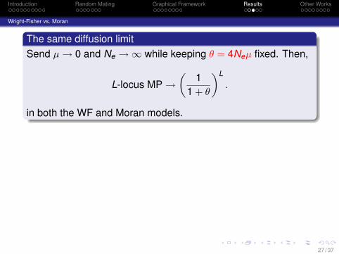
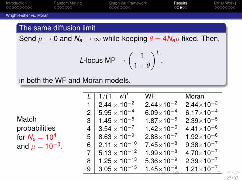
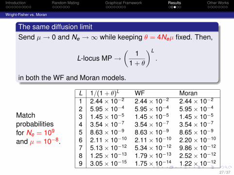
The same diffusion limitSend µ → 0 and Ne →∞ while keeping θ = 4Neµ fixed. Then,
L-locus MP →(
11 + θ
)L
.
in both the WF and Moran models.
27 / 37
Introduction Random Mating Graphical Framework Results Other Works
Wright-Fisher vs. Moran
The same diffusion limitSend µ → 0 and Ne →∞ while keeping θ = 4Neµ fixed. Then,
L-locus MP →(
11 + θ
)L
.
in both the WF and Moran models.
Matchprobabilitiesfor Ne = 104
and µ = 10−3.
L 1/(1 + θ)L WF Moran1 2.44× 10⁻² 2.44×10⁻² 2.44×10⁻²
2 5.95× 10⁻⁴ 6.09×10⁻⁴ 6.17×10⁻⁴
3 1.45× 10⁻⁵ 1.87×10⁻⁵ 2.39×10⁻⁵
4 3.54× 10⁻⁷ 1.42×10⁻⁶ 4.41×10⁻⁶
5 8.63× 10⁻⁹ 2.88×10⁻⁷ 1.92×10⁻⁶
6 2.11× 10⁻¹⁰ 7.45×10⁻⁸ 9.38×10⁻⁷
7 5.13× 10⁻¹² 1.99×10⁻⁸ 4.70×10⁻⁷
8 1.25× 10⁻¹³ 5.36×10⁻⁹ 2.39×10⁻⁷
9 3.05× 10⁻¹⁵ 1.45×10⁻⁹ 1.21×10⁻⁷
27 / 37
Introduction Random Mating Graphical Framework Results Other Works
Wright-Fisher vs. Moran
The same diffusion limitSend µ → 0 and Ne →∞ while keeping θ = 4Neµ fixed. Then,
L-locus MP →(
11 + θ
)L
.
in both the WF and Moran models.
Matchprobabilitiesfor Ne = 109
and µ = 10−8.
L 1/(1 + θ)L WF Moran1 2.44× 10⁻² 2.44× 10⁻² 2.44× 10⁻²
2 5.95× 10⁻⁴ 5.95× 10⁻⁴ 5.95× 10⁻⁴
3 1.45× 10⁻⁵ 1.45× 10⁻⁵ 1.45× 10⁻⁵
4 3.54× 10⁻⁷ 3.54× 10⁻⁷ 3.54× 10⁻⁷
5 8.63× 10⁻⁹ 8.63× 10⁻⁹ 8.65× 10⁻⁹
6 2.11× 10⁻¹⁰ 2.11× 10⁻¹⁰ 2.20× 10⁻¹⁰
7 5.13× 10⁻¹² 5.34× 10⁻¹² 9.86× 10⁻¹²
8 1.25× 10⁻¹³ 1.79× 10⁻¹³ 2.52× 10⁻¹²
9 3.05× 10⁻¹⁵ 1.75× 10⁻¹⁴ 1.22× 10⁻¹²
27 / 37
Introduction Random Mating Graphical Framework Results Other Works
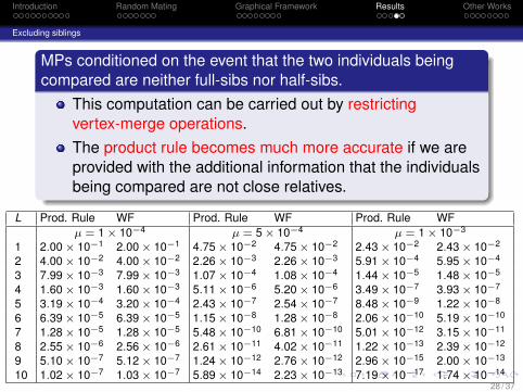
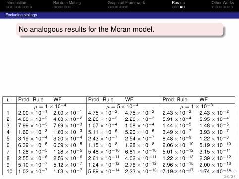
Excluding siblings
MPs conditioned on the event that the two individuals beingcompared are neither full-sibs nor half-sibs.
This computation can be carried out by restrictingvertex-merge operations.The product rule becomes much more accurate if we areprovided with the additional information that the individualsbeing compared are not close relatives.
L Prod. Rule WF Prod. Rule WF Prod. Rule WFµ = 1 × 10⁻⁴ µ = 5 × 10⁻⁴ µ = 1 × 10⁻³
1 2.00 × 10⁻¹ 2.00 × 10⁻¹ 4.75 × 10⁻² 4.75 × 10⁻² 2.43 × 10⁻² 2.43 × 10⁻²
2 4.00 × 10⁻² 4.00 × 10⁻² 2.26 × 10⁻³ 2.26 × 10⁻³ 5.91 × 10⁻⁴ 5.95 × 10⁻⁴
3 7.99 × 10⁻³ 7.99 × 10⁻³ 1.07 × 10⁻⁴ 1.08 × 10⁻⁴ 1.44 × 10⁻⁵ 1.48 × 10⁻⁵
4 1.60 × 10⁻³ 1.60 × 10⁻³ 5.11 × 10⁻⁶ 5.20 × 10⁻⁶ 3.49 × 10⁻⁷ 3.93 × 10⁻⁷
5 3.19 × 10⁻⁴ 3.20 × 10⁻⁴ 2.43 × 10⁻⁷ 2.54 × 10⁻⁷ 8.48 × 10⁻⁹ 1.22 × 10⁻⁸
6 6.39 × 10⁻⁵ 6.39 × 10⁻⁵ 1.15 × 10⁻⁸ 1.28 × 10⁻⁸ 2.06 × 10⁻¹⁰ 5.19 × 10⁻¹⁰
7 1.28 × 10⁻⁵ 1.28 × 10⁻⁵ 5.48 × 10⁻¹⁰ 6.81 × 10⁻¹⁰ 5.01 × 10⁻¹² 3.15 × 10⁻¹¹
8 2.55 × 10⁻⁶ 2.56 × 10⁻⁶ 2.61 × 10⁻¹¹ 4.02 × 10⁻¹¹ 1.22 × 10⁻¹³ 2.39 × 10⁻¹²
9 5.10 × 10⁻⁷ 5.12 × 10⁻⁷ 1.24 × 10⁻¹² 2.76 × 10⁻¹² 2.96 × 10⁻¹⁵ 2.00 × 10⁻¹³
10 1.02 × 10⁻⁷ 1.03 × 10⁻⁷ 5.89 × 10⁻¹⁴ 2.23 × 10⁻¹³ 7.19 × 10⁻¹⁷ 1.74 × 10⁻¹⁴
28 / 37
Introduction Random Mating Graphical Framework Results Other Works
Excluding siblings
No analogous results for the Moran model.
L Prod. Rule WF Prod. Rule WF Prod. Rule WFµ = 1 × 10⁻⁴ µ = 5 × 10⁻⁴ µ = 1 × 10⁻³
1 2.00 × 10⁻¹ 2.00 × 10⁻¹ 4.75 × 10⁻² 4.75 × 10⁻² 2.43 × 10⁻² 2.43 × 10⁻²
2 4.00 × 10⁻² 4.00 × 10⁻² 2.26 × 10⁻³ 2.26 × 10⁻³ 5.91 × 10⁻⁴ 5.95 × 10⁻⁴
3 7.99 × 10⁻³ 7.99 × 10⁻³ 1.07 × 10⁻⁴ 1.08 × 10⁻⁴ 1.44 × 10⁻⁵ 1.48 × 10⁻⁵
4 1.60 × 10⁻³ 1.60 × 10⁻³ 5.11 × 10⁻⁶ 5.20 × 10⁻⁶ 3.49 × 10⁻⁷ 3.93 × 10⁻⁷
5 3.19 × 10⁻⁴ 3.20 × 10⁻⁴ 2.43 × 10⁻⁷ 2.54 × 10⁻⁷ 8.48 × 10⁻⁹ 1.22 × 10⁻⁸
6 6.39 × 10⁻⁵ 6.39 × 10⁻⁵ 1.15 × 10⁻⁸ 1.28 × 10⁻⁸ 2.06 × 10⁻¹⁰ 5.19 × 10⁻¹⁰
7 1.28 × 10⁻⁵ 1.28 × 10⁻⁵ 5.48 × 10⁻¹⁰ 6.81 × 10⁻¹⁰ 5.01 × 10⁻¹² 3.15 × 10⁻¹¹
8 2.55 × 10⁻⁶ 2.56 × 10⁻⁶ 2.61 × 10⁻¹¹ 4.02 × 10⁻¹¹ 1.22 × 10⁻¹³ 2.39 × 10⁻¹²
9 5.10 × 10⁻⁷ 5.12 × 10⁻⁷ 1.24 × 10⁻¹² 2.76 × 10⁻¹² 2.96 × 10⁻¹⁵ 2.00 × 10⁻¹³
10 1.02 × 10⁻⁷ 1.03 × 10⁻⁷ 5.89 × 10⁻¹⁴ 2.23 × 10⁻¹³ 7.19 × 10⁻¹⁷ 1.74 × 10⁻¹⁴
28 / 37
Introduction Random Mating Graphical Framework Results Other Works
Excluding siblings
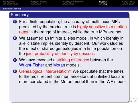
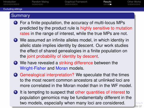
Summary1 For a finite population, the accuracy of multi-locus MPs
predicted by the product rule is highly sensitive to mutationrates in the range of interest, while the true MPs are not.
2 We assumed an infinite alleles model, in which identity inallelic state implies identity by descent. Our work studiesthe effect of shared genealogies in a finite population onthe joint probability of identity by descent.
3 We have revealed a striking difference between theWright-Fisher and Moran models.
4 Genealogical interpretation? We speculate that the timesto the most recent common ancestors at unlinked loci aremore correlated in the Moran model than in the WF model.
5 It is tempting to suspect that other quantities of interest topopulation genomics may be fundamentally different in thetwo models, especially when many loci are considered.
29 / 37
Introduction Random Mating Graphical Framework Results Other Works
Excluding siblings
Summary1 For a finite population, the accuracy of multi-locus MPs
predicted by the product rule is highly sensitive to mutationrates in the range of interest, while the true MPs are not.
2 We assumed an infinite alleles model, in which identity inallelic state implies identity by descent. Our work studiesthe effect of shared genealogies in a finite population onthe joint probability of identity by descent.
3 We have revealed a striking difference between theWright-Fisher and Moran models.
4 Genealogical interpretation? We speculate that the timesto the most recent common ancestors at unlinked loci aremore correlated in the Moran model than in the WF model.
5 It is tempting to suspect that other quantities of interest topopulation genomics may be fundamentally different in thetwo models, especially when many loci are considered.
29 / 37
Introduction Random Mating Graphical Framework Results Other Works
Outline1 Introduction
Random match probabilityCold hit
2 Models of Random MatingRecurrence equations
3 Graphical FrameworkMatch graphsOperations on graphsTopological ordering and graph enumeration
4 ResultsAccuracy of the product ruleWright-Fisher vs. MoranExcluding siblings
5 Other WorksPerfect Monogamy ModelSubdivided populationsFamilial search
29 / 37
Introduction Random Mating Graphical Framework Results Other Works
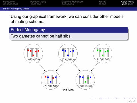
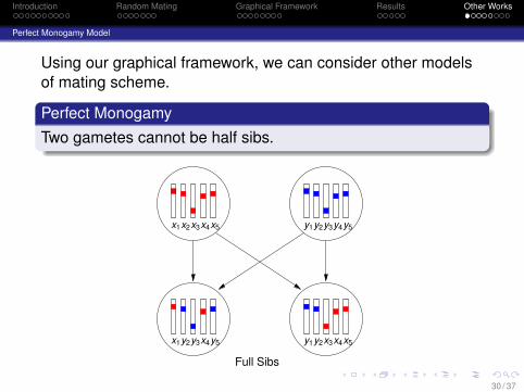
Perfect Monogamy Model
Using our graphical framework, we can consider other modelsof mating scheme.
Perfect MonogamyTwo gametes cannot be half sibs.
Half Sibs
y1 y3y4y5y2
x1 y3x4y5y2
z1 z3z4z5z2x1 x3x4x5x2
y1 z3z4y5y2
30 / 37
Introduction Random Mating Graphical Framework Results Other Works
Perfect Monogamy Model
Using our graphical framework, we can consider other modelsof mating scheme.
Perfect MonogamyTwo gametes cannot be half sibs.
Full Sibs
y1 y3y4y5y2
x1 y3x4y5y2
x1 x3x4x5x2
y1 x3x4x5y2
30 / 37
Introduction Random Mating Graphical Framework Results Other Works
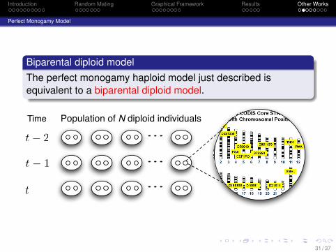
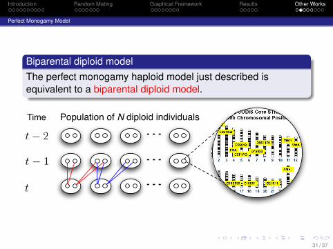
Perfect Monogamy Model
Biparental diploid modelThe perfect monogamy haploid model just described isequivalent to a biparental diploid model.
Population of N diploid individuals
t! 1
Time
t
t! 2
31 / 37
Introduction Random Mating Graphical Framework Results Other Works
Perfect Monogamy Model
Biparental diploid modelThe perfect monogamy haploid model just described isequivalent to a biparental diploid model.
Population of N diploid individuals
t! 1
Time
t
t! 2
31 / 37
Introduction Random Mating Graphical Framework Results Other Works
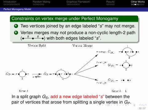
Perfect Monogamy Model
Constraints on vertex merge under Perfect Monogamy1 Two vertices joined by an edge labeled “s” may not merge.2 Vertex merges may not produce a non-cyclic length-2 path
(• s • s •) with both edges labeled “s”.
GP = x y12 GS =w x y zs s1 2w x y z1 2x y12x y
GM1 =GM2 =GM3 =2 splits0 merge2 merges2 merges
Vertex Split Vertex Mergetime t time t� 1
In a split graph GS, add a new edge labeled “s” between thepair of vertices that arose from splitting a single vertex in GP .
32 / 37
Introduction Random Mating Graphical Framework Results Other Works
Perfect Monogamy Model
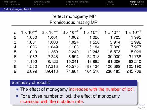
Perfect monogamy MPPromiscuous mating MP
µL 1× 10⁻⁴ 2× 10⁻⁴ 3× 10⁻⁴ 1× 10⁻³ 1× 10⁻² 1× 10⁻¹
2 1.000 1.001 1.002 1.026 1.723 1.9953 1.001 1.008 1.024 1.556 3.914 3.9924 1.006 1.049 1.188 5.184 7.828 7.9775 1.019 1.259 2.240 12.248 15.573 15.9296 1.062 2.246 6.994 24.018 30.930 31.7687 1.192 6.122 19.341 45.882 61.286 63.2108 1.580 17.218 40.575 87.134 120.899 125.1909 2.699 39.413 74.664 164.510 236.485 245.708
Summary of resultsThe effect of monogamy increases with the number of loci.For a given number of loci, the effect of monogamyincreases with the mutation rate.
33 / 37
Introduction Random Mating Graphical Framework Results Other Works
Perfect Monogamy Model
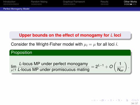
Upper bounds on the effect of monogamy for L loci
Consider the Wright-Fisher model with µi = µ for all loci i .
Proposition
limµ↑1
L-locus MP under perfect monogamyL-locus MP under promiscuous mating
= 2L−1 + O(
1NWF
).
34 / 37
Introduction Random Mating Graphical Framework Results Other Works
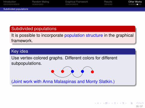
Subdivided populations
Subdivided populationsIt is possible to incorporate population structure in the graphicalframework.
Key ideaUse vertex-colored graphs. Different colors for differentsubpopulations.
(Joint work with Anna Malaspinas and Monty Slatkin.)
35 / 37
Introduction Random Mating Graphical Framework Results Other Works
Familial search
Recent California policy on familial searchCalifornia recently implemented a policy for using partialDNA matches to identify potential close relatives of theindividual who left a crime-scene sample.In addition to the 13-locus CODIS profiles, the policy alsocalls for using Y-linked markers to provide further evidenceof relatedness.We just submitted a paper on the population geneticsconsequences of the policy. Specifically, we have anestimate on the number and ethnic distribution of falseleads.(Joint work with Erin Murphy and Monty Slatkin.)
36 / 37
Introduction Random Mating Graphical Framework Results Other Works
Familial search
Thank you for your attention.
Acknowledgments
UC BerkeleyMonty Slatkin (Integrative Biology)Erin Murphy (School of Law)Anand Bhaskar (Computer Science)Anna Malaspinas (Integrative Biology)
Research supported in part by NIH, NSF, Alfred P. Sloan Research Fellowship, and
Packard Fellowship for Science and Engineering
37 / 37