Embed Size (px)
Citation preview
1
Forecasting Trends in Recorded Crime
January 2001
Derek Deadman
Public Sector Econom ics Research Centre
University of Leicester
ABSTRACT
There is an extensive literature on the modelling of property crime but little of this literature has attempted to use the estimated models for forecasting. A recent exception is the published Home Officepredictions of recorded burglary and theft for 1999 to 2001. These Home Office predictions (which are for a reversal of the recentdownward trend in recorded offences) are compared here withalternative econometric and multivariate time series predictions. The crucial role of the error correction structure of the econometricestimates compared with the forecast profiles which come from time series approaches is highlighted. Diaggregation of theft into vehicle and non vehicle crime is seen as potentially a fruitful area for furtherresearch.
2
Introduction
This study is concerned with forecasting issues relating to the recorded offences of Burglary and of Theft and Handling of Stolen Goods in England and W ales between 1999 and 2001. The forecasting exercise is intended:
1) To develop econometric models, based upon past research in PSERC, but applied to the same burglary and theft categories analysed by Dhiri et al(1999), hereafter referred to as HORS 198.
2) To use these models to produce forecasts directly comparable with those in HORS 198.
3) To isolate the main elements underlying the projected change in crime and the difference in the projections made by the Home Office and PSERC teams.
Statistical time-series forecasting methods (Box-Jenkins ARIM A modelling and transfer function analysis) are used as comparators for the econometric error-correction approach. Transfer function modelling is used to isolate the contribution of economic and demographic influences from other factors (such as the feedback dynamics built into econometric error-correction models).
All forecasts for recorded crime have been made under the ‘old rules’ for counting offences rather than the ‘new rules’ recently introduced. Criminal Statistics (1998, p.31) suggests that the effect of the new counting rules will be minimal for recorded Burglary but that for 1998 have raised Theft by 65,000 recorded offences compared to the old rules.
Data used
Formal definitions of data used in this study are given in an Appendix to this paper. From 1969 (that is, following the Theft Act, 1968), data used for Burglary and Theft and Handling of Stolen Goods were as used in HORS 198. Data from Criminal Statistics for 1950-1968 inclusive on the investigated crime categories was used for the earlier period rather than the ‘adjusted’ series used in HORS 198. The analysis here uses a dummy variable to model the break in the series, an approach used in our earlier work (Pudney, Deadman and Pyle (2000)). The consumption series used in HORS 198 was also used in this study. Our demographic variable is based on the number of young men in England and W ales aged 15-24 as a proportion of the population of England and W ales. Crim inal justice variables (police numbers, conviction rates, probability of imprisonment and length of sentence) follow those used in Pudney, Deadman and Pyle (2000) and by Deadman and Pyle in M acdonald and Pyle (2000).
Problems identified in HORS 198
W ithin this study and in Pudney (2000) we have also considered several problems identified in the HORS 198 study, namely:
3
1) W hether ‘single equation’ modelling approaches which ignore potential feedback between recorded crime and the set of criminal justice variablesare appropriate in this area. (This is related to the 'Policy Variable’ issue HORS 198, pp 11/12).
2) The relative weakness of the Theft model compared to that for Burglary and the possible need to disaggregate this category (HORS 198, p.21)
3) The problem of the wide confidence intervals for forecasts making the forecasting of more than 3 years ahead problematical (HORS 198, p.18).
Econometric Estimation
The use of single-equation error-correction econometric approaches to model and forecast crime has now become quite common. Such modelling is normally preceded by an examination of the orders of integration of the variables used. The orders of integration of the variables used here have been previously established (generally I(1)) in HORS 198 and in Pudney, Deadman and Pyle (2000). Pudney, Deadman and Pyle (1997) demonstrated the superiority of the Sims, Stock and W atson estimation technique over the Engle-Granger method for models with a single cointegrating vector. It is worth considering, however, whether single-equation approaches are appropriate for modelling crime.
As is now generally accepted, residual-based cointegration tests such as the Engle-Granger procedure which assume a maximum of one cointegrating vector are less efficient than the multivariate approach of Johansen which allows for multiple cointegrating vectors. Additionally, the development of the Johansen test described in Pesaran and Pesaran (1997) which allows for the determination of the number of cointegrating vectors in the presence of ‘long run forcing variables’ – i.e. exogenous variables– seems particularly suited to the problems considered here. That is, the suggestion that the criminal justice variables may exhibit feedback effects with recorded crime (and indeed, each other) may be investigated in the presence of other variables– consumption, unemployment and the demographic variable – which are clearly determined outside of the system being investigated. The rather short series of data employed in this study (annual data 1950 – 1998) precludes extensive testing, but the results of the econometric exercise still appear informative.
Burglary
The Johansen approach involves the estimation of a Vector Autoregressive M odel (VAR). The selection of the order of this VAR is the first consideration. Even if one starts with an overparametized (given the sample length) unrestricted VAR(4) model, the Schwarz Bayesian Criterion (SBC) uniformly points to a VAR(1) model being appropriate. As is often the case, the Akaike Information Criterion (AIC) points to a higher value for the order of the VAR, but experiments with higher orders lead to an ambiguous or uninformative choice for the number of cointegrating vectors. Peseran and Peseran (1997, p.277 and p.297) suggest choosing the lower value for the order of the VAR where there are low degrees of freedom. Serial correlation in the residuals of
4
the individual unrestricted VAR equations was not generally indicated, though the burglary equation was an exception ( )1(2c = 7.257).
However, for a cointegrating VAR(1) model, the number of cointegrating vectors is indicated as one by all the primary test statistics (trace, eigenvalue, AIC and SBC) for a model estimated with restricted intercepts and no deterministic trends. The error-correction equations suggest that a sensible model may be constructed for recorded Burglary but not for the other potentially endogenous criminal justice variables. This parallels the finding established for Residential Burglary reported in Deadman (2000). Simultaneity within the criminal justice variables does not appear to be a problem here and thus there is justification for building a single-equation error-correction model for Burglary (Darnell (1994, p.116 or Charemza and Deadman (1997, p.178)).
One approach to building such a model is to start from a completely general Autoregressive Distributed Lag (ADL) model which includes lags for all variables in the model. Given the short data series and the number of explanatory variables used, an initial model involving two lags in the level of the dependent variable and a single lag for each explanatory variable was adopted. This was recast into an error correction form and then estimated using the Sims, Stock and W atson method. Table 1 reports thisestimated model.

5
TABLE 1Ordinary Least Squares EstimationDependent Variable is ∆Burglary
General M odelAll variables in natural logarithms
Coefficient t-ratio P-value∆ Consum ption -0.9744 -1.6627 0.108∆ Conviction -0.4517 -3.1553 0.004∆ Dummy 0.2098 3.2994 0.003∆ Imprisonment -0.2093 -2.4978 0.019∆ Police -2.1641 -2.6622 0.013∆ Sentence 0.0557 0.6192 0.541∆ Unemployment 0.2128 3.4079 0.002∆ Youths 1.6759 1.5695 0.128Burglary (-1) -0.2425 10.5313 0.000∆ Burglary (-1) 0.2167 2.6835 0.012Consumption (-1) 1.1791 3.8425 0.001Conviction (-1) 0.0065 0.0453 0.964Dummy 0.1252 2.1019 0.045Imprisonment (-1) -0.1038 -1.1905 0.244Intercept -11.4531 -2.8815 0.008Police (-1) -1.5199 -2.4540 0.021Sentence (-1) -0.2550 -2.1056 0.044Unemployment (-1) 0.0291 0.5714 0.572Youths (-1) 0.3037 1.0971 0.282
Notes:
47 Observations used for estimation from 1952 to 1998. All variables in natural logarithms.
R2 = 0.90105 R-Bar–Squared = 0.83743S.E. of Regression = 0.04446 F-Stat. F(18, 28) 14.1645 (.000)M ean of Dep Var = 0.04558 S.D. of Dep Var = 011027RSS = 0.055343 Equation Log-likelihood = 91.802Akaike Info. Criterion = 72.802 Schwarz Bayesian Criterion = 55.2256DW Statistic 2.1343 Durbin’s h-statistic = -.5528 (.580)
Serial Correlation )1(2c = 0.43939 (.507) F(1, 27) = 0.255 (.618)
Functional Form )1(2c = 0.5896 (.443) F(1, 27) = 0.3430 (.563)
Normality )2(2c = 0.7704 (.680) Not Applicable
Heteroscedasticity )1(2c = 0.04229 (.837) F(1, 45) = 0.041 (.841)
6
This model provides a good fit to the sample data and passes the standard diagnostic tests. The estimated coefficients of the criminal justice variables indicate a significantdeterrence role for these variables, and both unemployment and consumption appear to have some explanatory power.
For prediction from this estimated model and those used subsequently, some assumptions need to be made regarding the values of the explanatory variables outside of the sample period. These were as follows:
Assum ption 1. All criminal justice variables (conviction rate, probability ofimprisonment, sentence length, number of police) were set at their values in 1998.
Assum ption2.Population projections (both for totals and for the number of males aged 15-24) were taken from GAD (1999).
Totals:UK 1996(base) 58,801,000 2001 59,618,000England and W ales 1996 (base) 52,010,000 2001 52,818,000
M ale Youths:England and W ales 1996 (base) 3,290,000 2001 3,297,000
Assum ption 3.Forecasts for household consumption are Treasury forecasts used in HORS 198.
Household consumption (percentage change from previous year)
1999 2.25% 2000 2.75% 2001 3%
Assum ption 4.Forecasts for unemployment are those made by the National Institute of Economic and Social Research (NIESR, (2000)).
Unemployment (Claimant Count)
1999 1,246,000 2000 1,180,000 2001 1,212,000
W hilst the demographic forecasts suggest only a small rise in the total number of males aged 15-24 years over the forecast period, this conceals a predicted 6% rise in the 15-19 year old age band compared to a 5% fall in the 20-24 year age band. If the former age group has a higher propensity to commit Burglary and Theft, the forecasts from this and subsequent models will tend to understate the demographic effect.
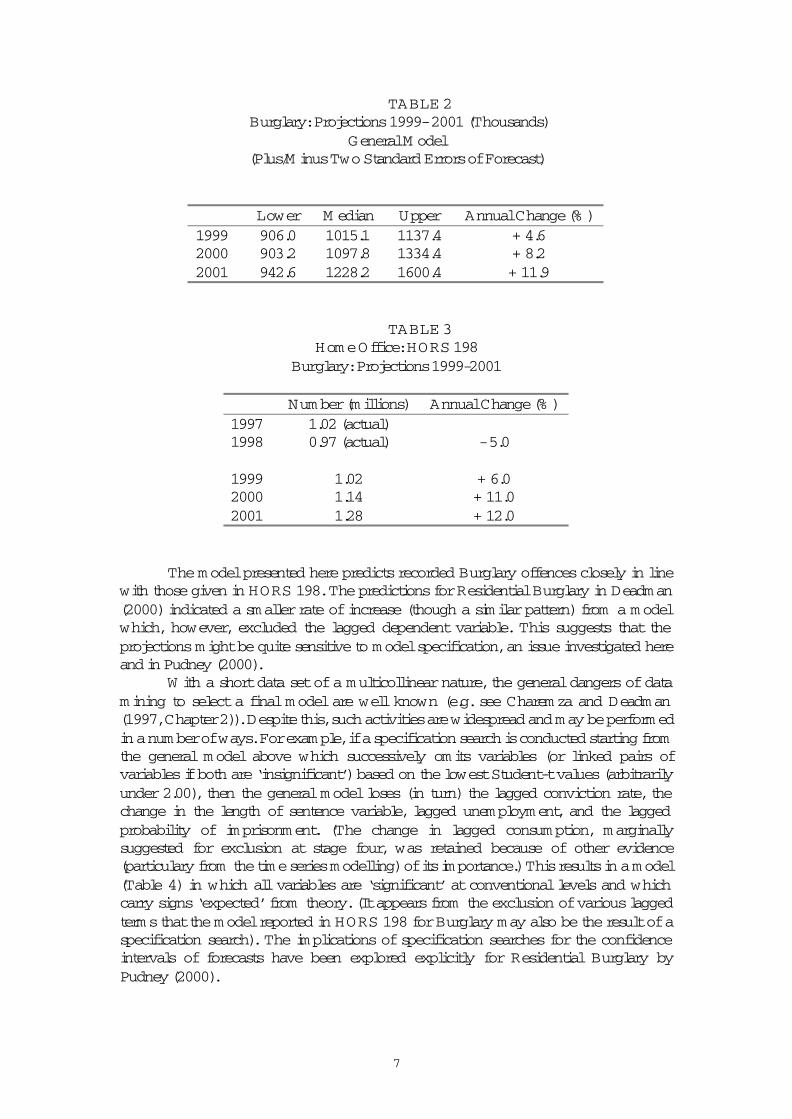
The dynamic forecasts for Burglary which result from the use of the assumptions and values above for the explanatory variables are given in Table 2 with the Home Office projections for Burglary in Table 3. The forecasts reported here and in later tables are made under the ‘old rules’ operated by the police for counting of offences rather than the new rules introduced in 1998.
7
TABLE 2 Burglary: Projections 1999- 2001 (Thousands)
General M odel(Plus/M inus Two Standard Errors of Forecast)
Lower M edian Upper Annual Change (% )1999 906.0 1015.1 1137.4 + 4.62000 903.2 1097.8 1334.4 + 8.22001 942.6 1228.2 1600.4 + 11.9
TABLE 3Home Office: HORS 198
Burglary: Projections 1999-2001
Number (millions) Annual Change (% )1997 1.02 (actual)1998 0.97 (actual) - 5.0
1999 1.02 + 6.02000 1.14 + 11.02001 1.28 + 12.0
The model presented here predicts recorded Burglary offences closely in line with those given in HORS 198. The predictions for Residential Burglary in Deadman (2000) indicated a smaller rate of increase (though a similar pattern) from a model which, however, excluded the lagged dependent variable. This suggests that the projections might be quite sensitive to model specification, an issue investigated here and in Pudney (2000).
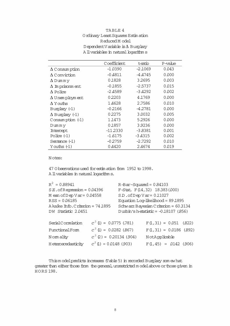
W ith a short data set of a multicollinear nature, the general dangers of data mining to select a final model are well known (e.g. see Charemza and Deadman (1997,Chapter 2)). Despite this, such activities are widespread and m ay be perform ed in a number of ways. For example, if a specification search is conducted starting from the general model above which successively omits variables (or linked pairs ofvariables if both are ‘insignificant’) based on the lowest Student-t values (arbitrarily under 2.00), then the general model loses (in turn) the lagged conviction rate, the change in the length of sentence variable, lagged unemployment, and the lagged probability of imprisonment. (The change in lagged consumption, marginallysuggested for exclusion at stage four, was retained because of other evidence(particulary from the time series modelling) of its importance.) This results in a model (Table 4) in which all variables are ‘significant’ at conventional levels and which carry signs ‘expected’ from theory. (It appears from the exclusion of various lagged terms that the model reported in HORS 198 for Burglary may also be the result of a specification search). The implications of specification searches for the confidence intervals of forecasts have been explored explicitly for Residential Burglary byPudney (2000).
8
TABLE 4Ordinary Least Squares Estimation
Reduced M odelDependent Variable is ∆ BurglaryAll variables in natural logarithms
Coefficient t-ratio P-value∆ Consum ption -1.0390 -2.1069 0.043∆ Conviction -0.4811 -4.4745 0.000∆ Dummy 0.1828 3.2695 0.003∆ Imprisonment -0.1855 -2.5737 0.015∆ Police -2.4589 -3.4292 0.002∆ Unemployment 0.2203 4.1769 0.000∆ Youths 1.4628 2.7586 0.010Burglary (-1) -0.2166 -4.2781 0.000∆ Burglary (-1) 0.2275 3.0032 0.005Consumption (-1) 1.1473 5.2926 0.000Dummy 0.1857 3.9236 0.000Intercept -11.2330 -3.8381 0.001Police (-1) -1.6175 -3.4315 0.002Sentence (-1) -0.2759 -2.7292 0.010Youths (-1) 0.4420 2.4674 0.019
Notes:
47 Observations used for estimation from 1952 to 1998. All variables in natural logarithms.
R2 = 0.88941 R-Bar–Squared = 0.84103S.E. of Regression = 0.04396 F-Stat. F(14, 32) 18.383(.000)M ean of Dep Var = 0.04558 S.D. of Dep Var = 0.11027RSS = 0.06185 Equation Log-likelihood = 89.1895Akaike Info. Criterion = 74.1895 Schwarz Bayesian Criterion = 60.3134DW Statistic 2.0451 Durbin’s h-statistic = -0.18107 (.856)
Serial Correlation )1(2c = 0.0775 (.781) F(1, 31) = 0.051 (.822)
Functional Form )1(2c = 0.0282 (.867) F(1, 31) = 0.0186 (.892)
Normality )2(2c = 0.20134 (.904) Not Applicable
Heteroscedasticity )1(2c = 0.0148 (.903) F(1, 45) = .0142 (.906)
This model predicts increases (Table 5) in recorded Burglary somewhat greater than either those from the general, unrestricted model above or those given in HORS 198.
9
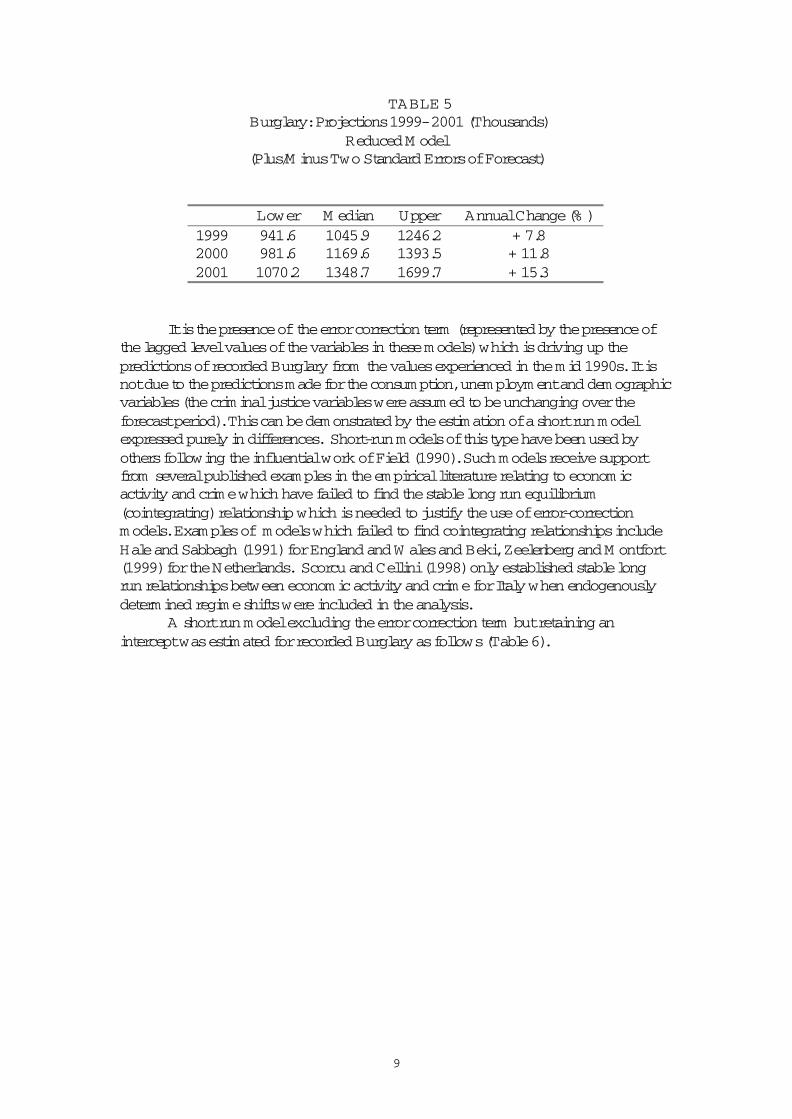
TABLE 5 Burglary: Projections 1999- 2001 (Thousands)
Reduced M odel(Plus/M inus Two Standard Errors of Forecast)
Lower M edian Upper Annual Change (% )1999 941.6 1045.9 1246.2 + 7.82000 981.6 1169.6 1393.5 + 11.82001 1070.2 1348.7 1699.7 + 15.3
It is the presence of the error correction term (represented by the presence of the lagged level values of the variables in these models) which is driving up the predictions of recorded Burglary from the values experienced in the mid 1990s. It is not due to the predictions made for the consumption, unemployment and demographic variables (the criminal justice variables were assumed to be unchanging over the forecast period). This can be demonstrated by the estimation of a short run model expressed purely in differences. Short-run models of this type have been used by others following the influential work of Field (1990). Such models receive support from several published examples in the empirical literature relating to economic activity and crime which have failed to find the stable long run equilibrium (cointegrating) relationship which is needed to justify the use of error-correctionmodels. Examples of models which failed to find cointegrating relationships include Hale and Sabbagh (1991) for England and W ales and Beki, Zeelenberg and M ontfort (1999) for the Netherlands. Scorcu and Cellini (1998) only established stable long run relationships between economic activity and crime for Italy when endogenously determined regime shifts were included in the analysis.
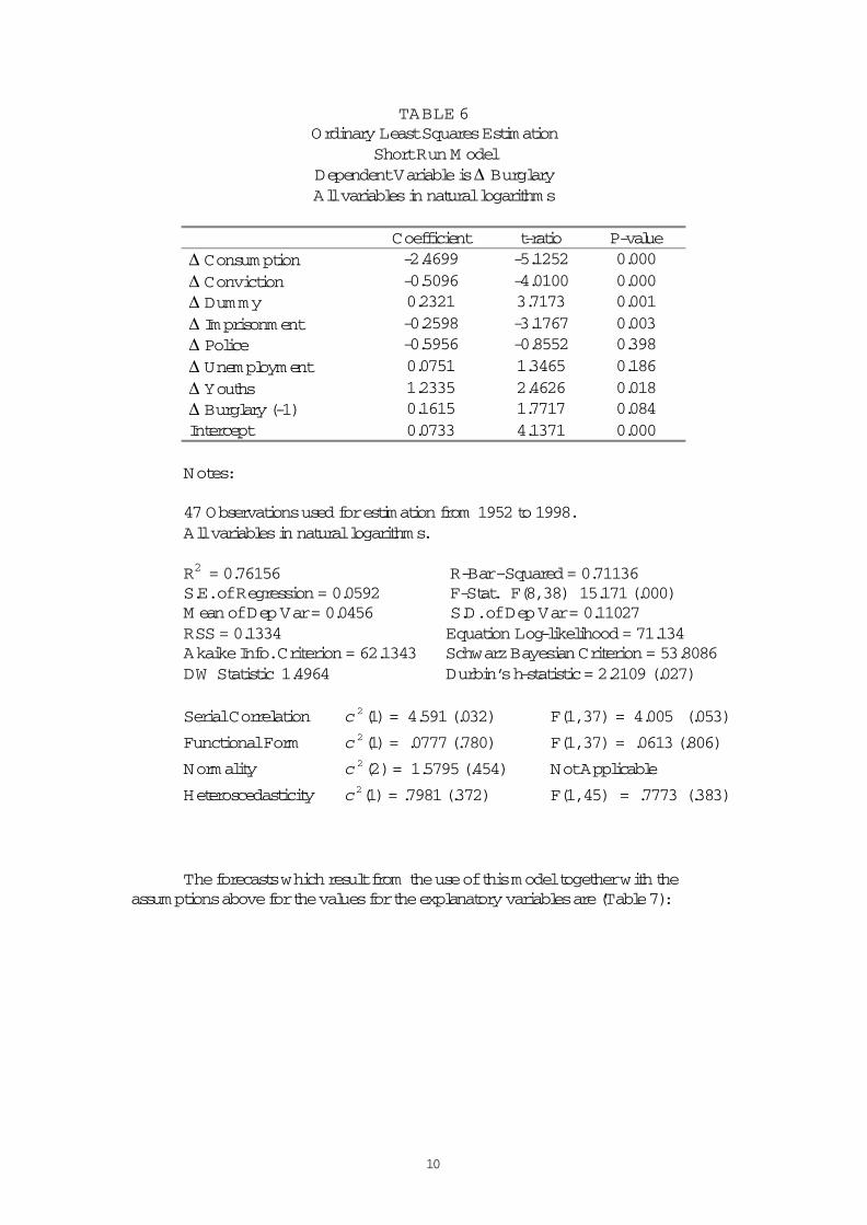
A short run model excluding the error correction term but retaining an intercept was estimated for recorded Burglary as follows (Table 6).
10
TABLE 6Ordinary Least Squares Estimation
Short Run M odelDependent Variable is ∆ BurglaryAll variables in natural logarithms
Coefficient t-ratio P-value∆ Consum ption -2.4699 -5.1252 0.000∆ Conviction -0.5096 -4.0100 0.000∆ Dummy 0.2321 3.7173 0.001∆ Imprisonment -0.2598 -3.1767 0.003∆ Police -0.5956 -0.8552 0.398∆ Unemployment 0.0751 1.3465 0.186∆ Youths 1.2335 2.4626 0.018∆ Burglary (-1) 0.1615 1.7717 0.084Intercept 0.0733 4.1371 0.000
Notes:
47 Observations used for estimation from 1952 to 1998. All variables in natural logarithms.
R2 = 0.76156 R-Bar–Squared = 0.71136S.E. of Regression = 0.0592 F-Stat. F(8, 38) 15.171 (.000)M ean of Dep Var = 0.0456 S.D. of Dep Var = 0.11027RSS = 0.1334 Equation Log-likelihood = 71.134Akaike Info. Criterion = 62.1343 Schwarz Bayesian Criterion = 53.8086DW Statistic 1.4964 Durbin’s h-statistic = 2.2109 (.027)
Serial Correlation )1(2c = 4.591 (.032) F(1, 37) = 4.005 (.053)
Functional Form )1(2c = .0777 (.780) F(1, 37) = .0613 (.806)
Normality )2(2c = 1.5795 (.454) Not Applicable
Heteroscedasticity )1(2c = .7981 (.372) F(1, 45) = .7773 (.383)
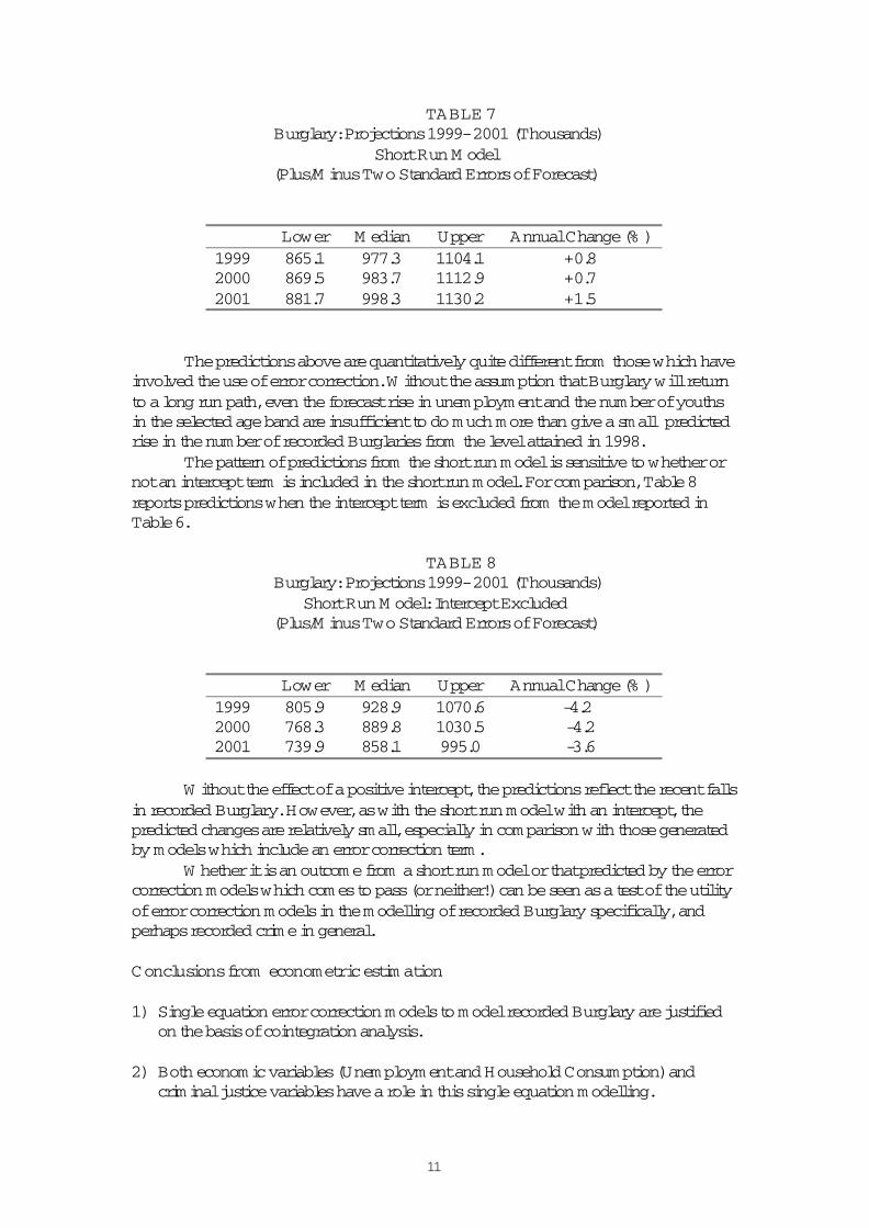
The forecasts which result from the use of this model together with the assumptions above for the values for the explanatory variables are (Table 7):
11
TABLE 7 Burglary: Projections 1999- 2001 (Thousands)
Short Run M odel(Plus/M inus Two Standard Errors of Forecast)
Lower M edian Upper Annual Change (% )1999 865.1 977.3 1104.1 +0.82000 869.5 983.7 1112.9 +0.72001 881.7 998.3 1130.2 +1.5
The predictions above are quantitatively quite different from those which have involved the use of error correction. W ithout the assumption that Burglary will return to a long run path, even the forecast rise in unemployment and the number of youths in the selected age band are insufficient to do much more than give a small predicted rise in the number of recorded Burglaries from the level attained in 1998.
The pattern of predictions from the short run model is sensitive to whether or not an intercept term is included in the short run model. For comparison, Table 8 reports predictions when the intercept term is excluded from the model reported in Table 6.
TABLE 8 Burglary: Projections 1999- 2001 (Thousands)
Short Run M odel: Intercept Excluded(Plus/M inus Two Standard Errors of Forecast)
Lower M edian Upper Annual Change (% )1999 805.9 928.9 1070.6 -4.22000 768.3 889.8 1030.5 -4.22001 739.9 858.1 995.0 -3.6
W ithout the effect of a positive intercept, the predictions reflect the recent falls in recorded Burglary. However, as with the short run model with an intercept, the predicted changes are relatively small, especially in comparison with those generated by models which include an error correction term.
W hether it is an outcome from a short run model or that predicted by the error correction models which comes to pass (or neither!) can be seen as a test of the utility of error correction models in the modelling of recorded Burglary specifically, and perhaps recorded crime in general.
Conclusions from econometric estim ation
1) Single equation error correction models to model recorded Burglary are justified on the basis of cointegration analysis.
2) Both economic variables (Unemployment and Household Consumption) and criminal justice variables have a role in this single equation modelling.

12
3) The disaggregation of recorded Burglary into Residential Burglary and Non-Residential Burglary is relatively unimportant in the forecast profile of this category, as judged by the results here in comparison with those in Deadman(2000).
4) The process of ‘reducing’ general models through specification searches results in models with quite different forecast levels over the forecast period, and leads to forecasts with wide confidence intervals.
5) The error correction specification in the single equation models is the principal reason for these models predicting rising recorded Burglary over the forecast period rather than the assumptions made about the future path of explanatory variables.
6) The differences between the variables used in HORS 198 and those used here in error correction models do not lead to substantial differences in the forecasts from the models. This suggests it is the dynamic structures of the models which is driving the forecasts.
Theft and Handling of Stolen Goods
HORS 198 (p.20) states that there is less confidence in the Theft model compared to that for Burglary. This finding is replicated in the results below.
Cointegration analysis
This analysis, carried out as described for Burglary above, failed to deliver a clear result on the number of cointegrating vectors involved in Theft. The analysis conducted with unrestricted intercepts and no trends provided no interpretable choice for the number of cointegrating vectors (r ) in any case where the order of the VARwas greater than one, and conflicting results (r = 1 or r = 2) for the VAR(1) model. The analysis for the preferred specification (that is, preferred on technical grounds(see Peseran and Peseran (1997), p.436)) which has restricted intercepts and no trendspointed to two cointegrating vectors, suggesting that a single equation approach to modelling Theft could be inappropriate.
Rather than pursue the analysis for the ‘all theft’ category (though for comparison, single equation results for this are included at the end of this section), it was thought to be potentially more rewarding to disaggregate this heterogeneous category. Vehicle crime is currently 50% of the total, but was only 12% in 1950. Additionally, vehicle crime typically does not involve prison sentences so that the criminal justice variables used when modelling ‘all theft’ are inappropriate for an important sub-group within the category.
Accordingly, besides producing forecasts for ‘all theft’ using what may be an inappropriate error correction single equation approach, we have done some introductory modelling of ‘non vehicle theft’ (all theft minus vehicle theft) and vehicle theft separately. M ore work needs to be done on these sub-groups, probably using a finer disaggregation than that considered here. As data on neither sentence length nor probability of imprisonment were available for non vehicle theft, the
13
corresponding data for ‘all theft’ were used as proxies. Both variables were excluded for vehicle crime.
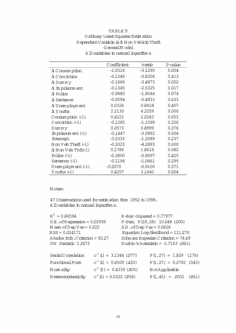
Cointegration analysis for non vehicle theft followed a pattern similar to that for the aggregate category. For a cointegrating VAR(1) model with restricted intercepts and no trends, two cointegrating vectors were indicated by eigenvalue, trace, SBC and HQC tests. Further analysis indicated that an error-correction equation for non vehicle theft could be established, but that the error-correction models for the other potentially ‘endogenous’ variables were uninformative. A parallel analysis of a model with unrestricted intercepts and no trends yielded similar results. Although the results indicate that a single equation model may be inappropriate in this case, whether /where the simultaneity exists within the group of criminal justice variables remains an unresolved issue.
The results of the estimation of a ‘general’ single equation error- correction model for non vehicle theft is given in Table 9 with the associated forecasts in Table 10. The corresponding results for a model for non vehicle theft arrived at after a specification search of the type discussed earlier are reported in Table 11 with corresponding forecasts in Table 12.
14
TABLE 9Ordinary Least Squares Estimation
Dependent Variable is ∆ Non Vehicle TheftGeneral M odel
All variables in natural logarithms
Coefficient t-ratio P-value∆ Consum ption -1.0316 -3.1290 0.004∆ Conviction -0.1246 -0.8306 0.413∆ Dummy -0.1666 -3.4873 0.002∆ Imprisonment -0.1345 -2.5325 0.017∆ Police -0.9880 -1.8544 0.074∆ Sentence -0.0594 -0.4833 0.633∆ Unemployment 0.0326 0.8418 0.407∆ Youths 2.2130 4.3259 0.000Consumption (-1) 0.4223 2.0243 0.053Conviction (-1) -0.1285 -1.1599 0.256Dummy 0.0573 0.8999 0.376Imprisonment (-1) -0.1447 -3.0892 0.004Intercept -3.5333 -1.2089 0.237Non Veh Theft (-1) -0.3023 -4.2893 0.000∆ Non Veh Thft(-1) 0.1786 1.8018 0.082Police (-1) -0.3800 -0.8097 0.425Sentence (-1) -0.1194 -1.0661 0.295Unemployment (-1) -0.0270 -0.9100 0.371Youths (-1) 0.4257 3.1640 0.004
Notes:
47 Observations used for estimation from 1952 to 1998.All variables in natural logarithms.
R2 = 0.86594 R-Bar–Squared = 0.77977S.E. of Regression = 0.02938 F-Stat. F(18, 28) 10.048 (.000)M ean of Dep Var = 0.022 S.D. of Dep Var = 0.0626
RSS = 0.024171 Equation Log-likelihood = 111.270Akaike Info. Criterion = 92.27 Schwarz Bayesian Criterion = 74.69DW Statistic 2.3673 Durbin’s h-statistic = -1.7163 (.861)
Serial Correlation )1(2c = 3.1344 (.077) F(1, 27) = 1.929 (.176)
Functional Form )1(2c = 0.6509 (.420) F(1, 27) = 0.3792 (.543)
Normality )2(2c = 0.4339 (.805) Not Applicable
Heteroscedasticity )1(2c = 0.0322 (.858) F(1, 45) = .0031 (.861)
15
TABLE 10 Non Vehicle Theft Projections 1999- 2001 (Thousands)
General M odel(Plus/M inus Two Standard Errors of Forecast)
Lower M edian Upper Annual Change (% )1999 1017.9 1111.1 1212.8 +4.4%2000 995.8 1157.7 1345.8 +4.2%2001 985.0 1204.5 1472.8 +4.0%
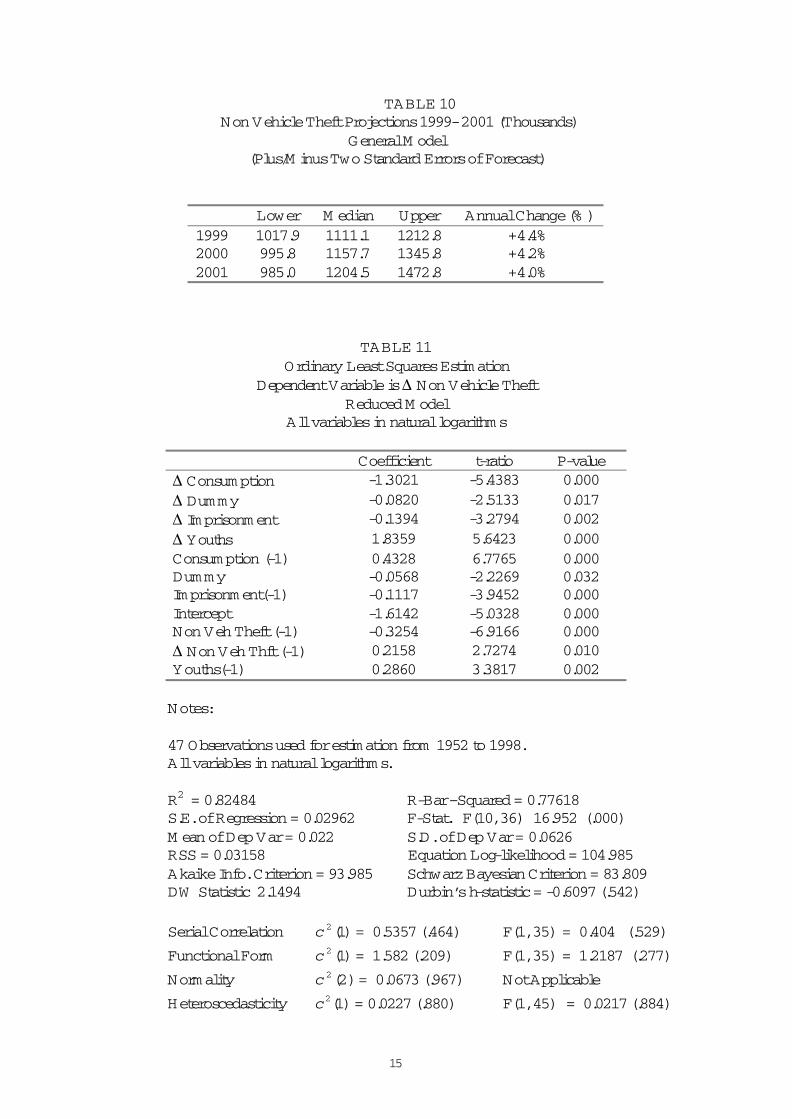
TABLE 11Ordinary Least Squares Estimation
Dependent Variable is ∆ Non Vehicle TheftReduced M odel
All variables in natural logarithms
Coefficient t-ratio P-value∆ Consum ption -1.3021 -5.4383 0.000∆ Dummy -0.0820 -2.5133 0.017∆ Imprisonment -0.1394 -3.2794 0.002∆ Youths 1.8359 5.6423 0.000Consumption (-1) 0.4328 6.7765 0.000Dummy -0.0568 -2.2269 0.032Imprisonment(-1) -0.1117 -3.9452 0.000Intercept -1.6142 -5.0328 0.000Non Veh Theft (-1) -0.3254 -6.9166 0.000∆ Non Veh Thft (-1) 0.2158 2.7274 0.010Youths(-1) 0.2860 3.3817 0.002
Notes:
47 Observations used for estimation from 1952 to 1998. All variables in natural logarithms.
R2 = 0.82484 R-Bar–Squared = 0.77618S.E. of Regression = 0.02962 F-Stat. F(10, 36) 16.952 (.000)M ean of Dep Var = 0.022 S.D. of Dep Var = 0.0626 RSS = 0.03158 Equation Log-likelihood = 104.985Akaike Info. Criterion = 93.985 Schwarz Bayesian Criterion = 83.809DW Statistic 2.1494 Durbin’s h-statistic = -0.6097 (.542)
Serial Correlation )1(2c = 0.5357 (.464) F(1,35) = 0.404 (.529)
Functional Form )1(2c = 1.582 (.209) F(1, 35) = 1.2187 (.277)
Normality )2(2c = 0.0673 (.967) Not Applicable
Heteroscedasticity )1(2c = 0.0227 (.880) F(1, 45) = 0.0217 (.884)
16
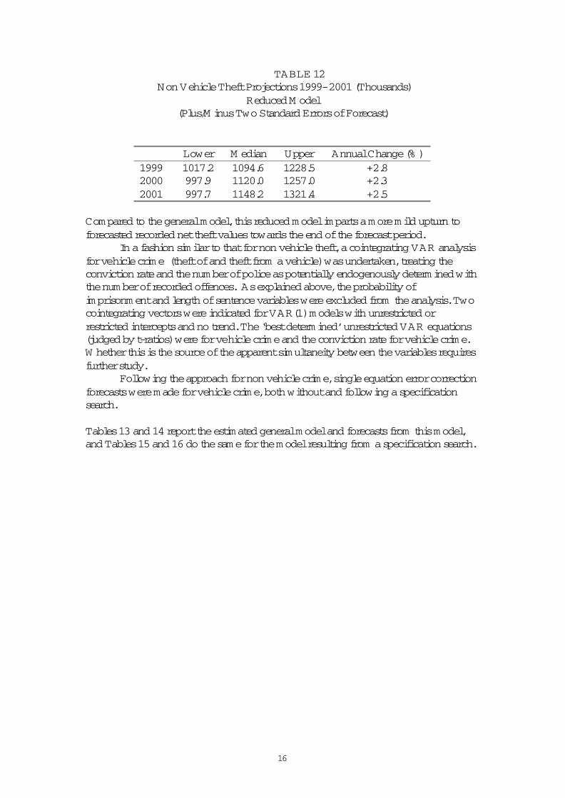
TABLE 12 Non Vehicle Theft Projections 1999- 2001 (Thousands)
Reduced M odel(Plus/M inus Two Standard Errors of Forecast)
Lower M edian Upper Annual Change (% )1999 1017.2 1094.6 1228.5 +2.82000 997.9 1120.0 1257.0 +2.32001 997.7 1148.2 1321.4 +2.5
Compared to the general model, this reduced model imparts a more mild upturn to forecasted recorded net theft values towards the end of the forecast period.
In a fashion similar to that for non vehicle theft, a cointegrating VAR analysis for vehicle crime (theft of and theft from a vehicle) was undertaken, treating the conviction rate and the number of police as potentially endogenously determined with the number of recorded offences. As explained above, the probability of imprisonment and length of sentence variables were excluded from the analysis. Two cointegrating vectors were indicated for VAR(1) models with unrestricted or restricted intercepts and no trend. The ‘best determined’ unrestricted VAR equations (judged by t-ratios) were for vehicle crime and the conviction rate for vehicle crime. W hether this is the source of the apparent simultaneity between the variables requires further study.
Following the approach for non vehicle crime, single equation error correction forecasts were made for vehicle crime, both without and following a specification search.
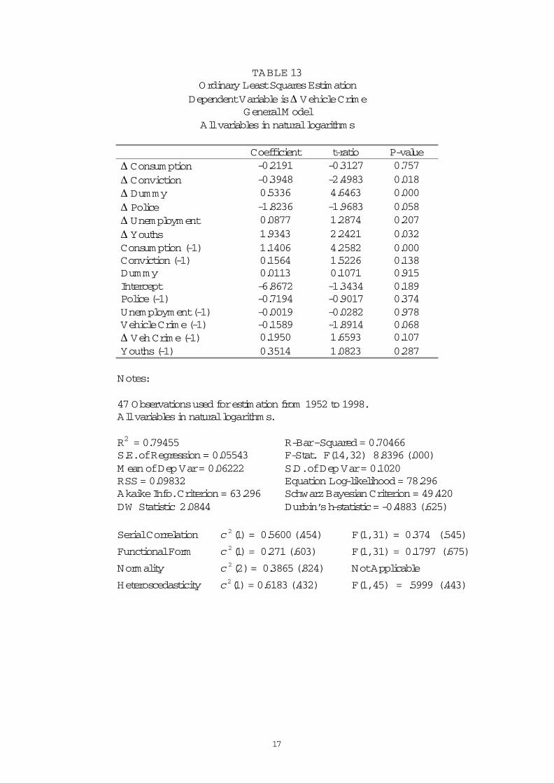
Tables 13 and 14 report the estimated general model and forecasts from this model, and Tables 15 and 16 do the same for the model resulting from a specification search.
17
TABLE 13Ordinary Least Squares Estimation
Dependent Variable is ∆ Vehicle CrimeGeneral M odel
All variables in natural logarithms
Coefficient t-ratio P-value∆ Consum ption -0.2191 -0.3127 0.757∆ Conviction -0.3948 -2.4983 0.018∆ Dummy 0.5336 4.6463 0.000∆ Police -1.8236 -1.9683 0.058∆ Unemployment 0.0877 1.2874 0.207∆ Youths 1.9343 2.2421 0.032Consumption (-1) 1.1406 4.2582 0.000Conviction (-1) 0.1564 1.5226 0.138Dummy 0.0113 0.1071 0.915Intercept -6.8672 -1.3434 0.189Police (-1) -0.7194 -0.9017 0.374Unemployment (-1) -0.0019 -0.0282 0.978Vehicle Crime (-1) -0.1589 -1.8914 0.068∆ Veh Crime (-1) 0.1950 1.6593 0.107Youths (-1) 0.3514 1.0823 0.287
Notes:
47 Observations used for estimation from 1952 to 1998. All variables in natural logarithms.
R2 = 0.79455 R-Bar–Squared = 0.70466S.E. of Regression = 0.05543 F-Stat. F(14, 32) 8.8396 (.000)M ean of Dep Var = 0.06222 S.D. of Dep Var = 0.1020RSS = 0.09832 Equation Log-likelihood = 78.296Akaike Info. Criterion = 63.296 Schwarz Bayesian Criterion = 49.420DW Statistic 2.0844 Durbin’s h-statistic = -0.4883 (.625)
Serial Correlation )1(2c = 0.5600 (.454) F(1, 31) = 0.374 (.545)
Functional Form )1(2c = 0.271 (.603) F(1, 31) = 0.1797 (.675)
Normality )2(2c = 0.3865 (.824) Not Applicable
Heteroscedasticity )1(2c = 0.6183 (.432) F(1, 45) = .5999 (.443)
18
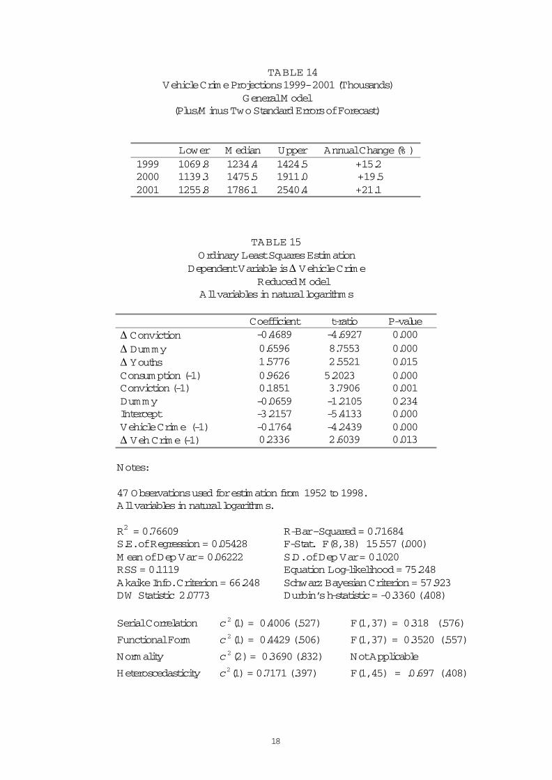
TABLE 14 Vehicle Crime Projections 1999- 2001 (Thousands)
General M odel(Plus/M inusTwo Standard Errors of Forecast)
Lower M edian Upper Annual Change (% )1999 1069.8 1234.4 1424.5 +15.22000 1139.3 1475.5 1911.0 +19.52001 1255.8 1786.1 2540.4 +21.1
TABLE 15Ordinary Least Squares Estimation
Dependent Variable is ∆ Vehicle CrimeReduced M odel
All variables in natural logarithms
Coefficient t-ratio P-value∆ Conviction -0.4689 -4.6927 0.000∆ Dummy 0.6596 8.7553 0.000∆ Youths 1.5776 2.5521 0.015Consumption (-1) 0.9626 5.2023 0.000Conviction (-1) 0.1851 3.7906 0.001Dummy -0.0659 -1.2105 0.234Intercept -3.2157 -5.4133 0.000Vehicle Crime (-1) -0.1764 -4.2439 0.000∆ Veh Crime (-1) 0.2336 2.6039 0.013
Notes:
47 Observations used for estimation from 1952 to 1998. All variables in natural logarithms.
R2 = 0.76609 R-Bar–Squared = 0.71684S.E. of Regression = 0.05428 F-Stat. F(8, 38) 15.557 (.000)M ean of Dep Var = 0.06222 S.D. of Dep Var = 0.1020RSS = 0.1119 Equation Log-likelihood = 75.248Akaike Info. Criterion = 66.248 Schwarz Bayesian Criterion = 57.923DW Statistic 2.0773 Durbin’s h-statistic = -0.3360 (.408)
Serial Correlation )1(2c = 0.4006 (.527) F(1, 37) = 0.318 (.576)
Functional Form )1(2c = 0.4429 (.506) F(1, 37) = 0.3520 (.557)
Normality )2(2c = 0.3690 (.832) Not Applicable
Heteroscedasticity )1(2c = 0.7171 (.397) F(1, 45) = .0.697 (.408)
19
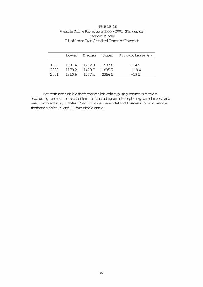
TABLE 16 Vehicle Crime Projections 1999- 2001 (Thousands)
Reduced M odel(Plus/M inus Two Standard Errors of Forecast)
Lower M edian Upper Annual Change (% )
1999 1081.4 1232.0 1537.8 +14.92000 1178.2 1470.7 1835.7 +19.42001 1310.6 1757.4 2356.5 +19.5
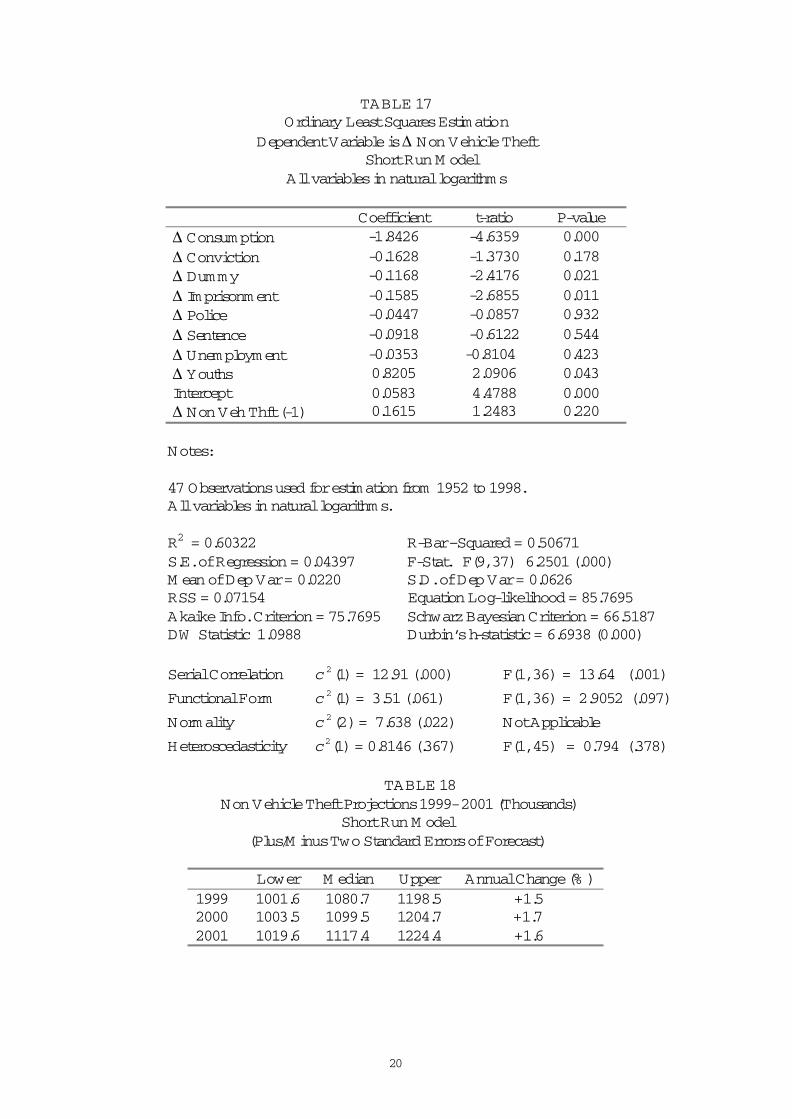
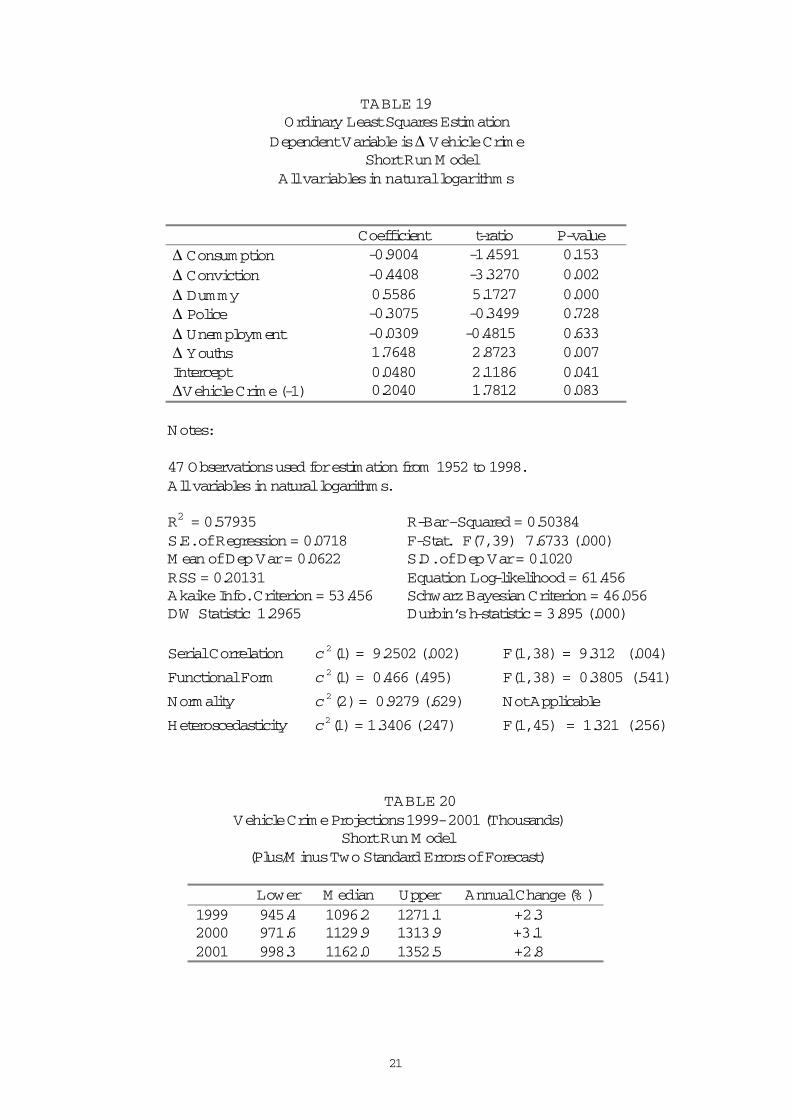
For both non vehicle theft and vehicle crime, purely short run models (excluding the error correction term but including an intercept) may be estimated and used for forecasting. Tables 17 and 18 give the model and forecasts for non vehicle theft and Tables 19 and 20 for vehicle crime.
20
TABLE 17Ordinary Least Squares Estimation
Dependent Variable is ∆ Non Vehicle TheftShort Run M odel
All variables in natural logarithms
Coefficient t-ratio P-value∆ Consum ption -1.8426 -4.6359 0.000∆ Conviction -0.1628 -1.3730 0.178∆ Dummy -0.1168 -2.4176 0.021∆ Imprisonment -0.1585 -2.6855 0.011∆ Police -0.0447 -0.0857 0.932∆ Sentence -0.0918 -0.6122 0.544∆ Unemployment -0.0353 -0.8104 0.423∆ Youths 0.8205 2.0906 0.043Intercept 0.0583 4.4788 0.000∆ Non Veh Thft (-1) 0.1615 1.2483 0.220
Notes:
47 Observations used for estimation from 1952 to 1998. All variables in natural logarithms.
R2 = 0.60322 R-Bar–Squared = 0.50671S.E. of Regression = 0.04397 F-Stat. F(9, 37) 6.2501 (.000)M ean of Dep Var = 0.0220 S.D. of Dep Var = 0.0626 RSS = 0.07154 Equation Log-likelihood = 85.7695Akaike Info. Criterion = 75.7695 Schwarz Bayesian Criterion = 66.5187DW Statistic 1.0988 Durbin’s h-statistic = 6.6938 (0.000)
Serial Correlation )1(2c = 12.91 (.000) F(1, 36) = 13.64 (.001)
FunctionalForm )1(2c = 3.51 (.061) F(1, 36) = 2.9052 (.097)
Normality )2(2c = 7.638 (.022) Not Applicable
Heteroscedasticity )1(2c = 0.8146 (.367) F(1, 45) = 0.794 (.378)
TABLE 18 Non Vehicle Theft Projections 1999- 2001 (Thousands)
Short Run M odel(Plus/M inus Two Standard Errors of Forecast)
Lower M edian Upper Annual Change (% )1999 1001.6 1080.7 1198.5 +1.52000 1003.5 1099.5 1204.7 +1.72001 1019.6 1117.4 1224.4 +1.6
21
TABLE 19Ordinary Least Squares Estimation
Dependent Variable is ∆ Vehicle Crime Short Run M odel
All variables in natural logarithm s
Coefficient t-ratio P-value∆ Consum ption -0.9004 -1.4591 0.153∆ Conviction -0.4408 -3.3270 0.002∆ Dummy 0.5586 5.1727 0.000∆ Police -0.3075 -0.3499 0.728∆ Unemployment -0.0309 -0.4815 0.633∆ Youths 1.7648 2.8723 0.007Intercept 0.0480 2.1186 0.041∆Vehicle Crime (-1) 0.2040 1.7812 0.083
Notes:
47 Observations used for estimation from 1952 to 1998. All variables in natural logarithms.
R2 = 0.57935 R-Bar–Squared = 0.50384S.E. of Regression = 0.0718 F-Stat. F(7, 39) 7.6733 (.000)M ean of Dep Var = 0.0622 S.D. of Dep Var = 0.1020RSS = 0.20131 Equation Log-likelihood = 61.456Akaike Info. Criterion = 53.456 Schwarz Bayesian Criterion = 46.056DW Statistic 1.2965 Durbin’s h-statistic = 3.895 (.000)
Serial Correlation )1(2c = 9.2502 (.002) F(1, 38) = 9.312 (.004)
Functional Form )1(2c = 0.466 (.495) F(1, 38) = 0.3805 (.541)
Normality )2(2c = 0.9279 (.629) Not Applicable
Heteroscedasticity )1(2c = 1.3406 (.247) F(1, 45) = 1.321 (.256)
TABLE 20 Vehicle Crime Projections 1999- 2001 (Thousands)
Short Run M odel(Plus/M inus Two Standard Errors of Forecast)
Lower M edian Upper Annual Change (% )1999 945.4 1096.2 1271.1 +2.32000 971.6 1129.9 1313.9 +3.12001 998.3 1162.0 1352.5 +2.8
22
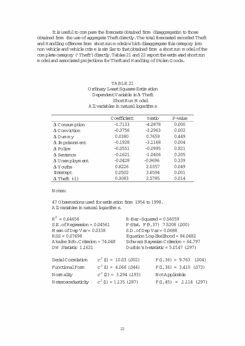
It is useful to compare the forecasts obtained from disaggregation to those obtained from the use of aggregate Theft directly. The total forecasted recorded Theft and Handling offences from short run models which disaggregate this category into non vehicle and vehicle crime is similar to that obtained from a short run model of the complete category (‘ Theft’) directly. Tables 21 and 22 report the estimated short run model and associated projections for Theft and Handling of Stolen Goods.
TABLE 21Ordinary Least Squares EstimationDependent Variable is ∆ Theft
ShortRun M odelAll variables in natural logarithms
Coefficient t-ratio P-value∆ Consum ption -1.7133 -4.2878 0.000∆ Conviction -0.3756 -3.2963 0.002∆ Dummy 0.0380 0.7659 0.449∆ Imprisonment -0.1928 -3.1168 0.004∆ Police -0.0551 -0.0995 0.921∆ Sentence -0.1621 -1.0406 0.305∆ Unemployment -0.0428 -0.9696 0.339∆ Youths 0.8226 2.0357 0.049Intercept 0.0502 3.6594 0.001∆ Theft (-1) 0.3083 2.5785 0.014
Notes:
47 Observations used for estimation from 1954 to 1998. All variables in natural logarithms.
R2 = 0.64656 R-Bar–Squared = 0.56059S.E. of Regression = 0.04561 F-Stat. F(9, 37) 7.5208 (.000)M ean of Dep Var = 0.0338 S.D. of Dep Var = 0.0688 RSS = 0.07698 Equation Log-likelihood = 84.0482Akaike Info. Criterion = 74.048 Schwarz Bayesian Criterion = 64.797DW Statistic 1.1621 Durbin’s h-statistic = 5.0147 (.297)
Serial Correlation )1(2c = 10.03 (.002) F(1, 36) = 9.763 (.004)
Functional Form )1(2c = 4.066 (.044) F(1, 36) = 3.410 (.073)
Normality )2(2c = 3.294 (.193) Not Applicable
Heteroscedasticity )1(2c = 1.135 (.287) F(1, 45) = .1.114 (.297)
23
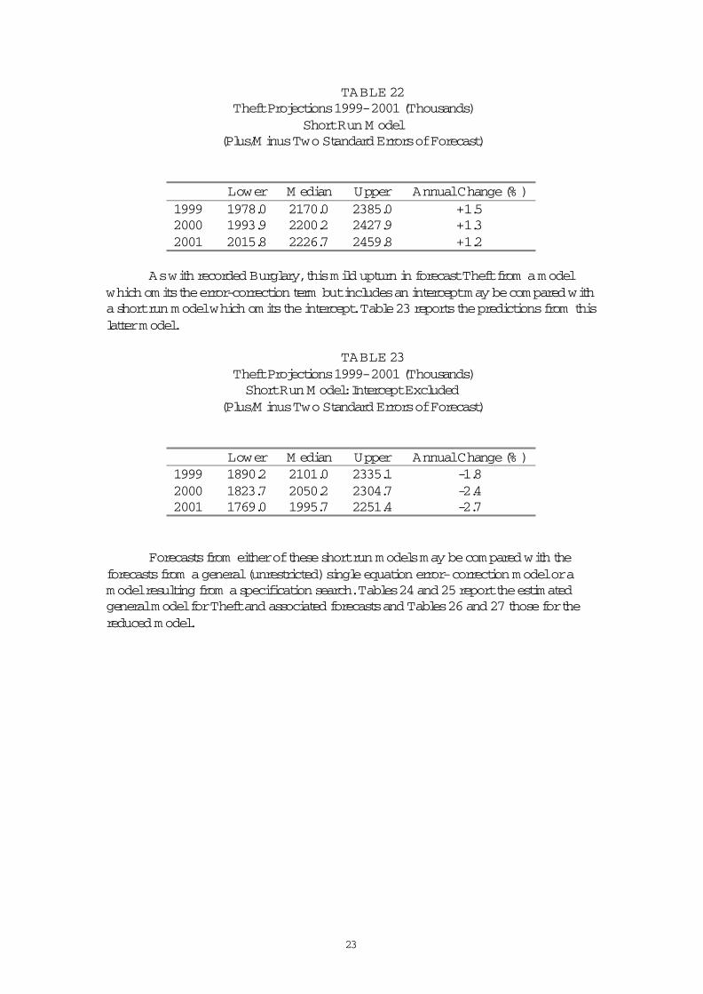
TABLE 22 Theft Projections 1999- 2001 (Thousands)
Short Run M odel(Plus/M inus Two Standard Errors of Forecast)
Lower M edian Upper Annual Change (% )1999 1978.0 2170.0 2385.0 +1.52000 1993.9 2200.2 2427.9 +1.32001 2015.8 2226.7 2459.8 +1.2
As with recorded Burglary, this mild upturn in forecast Theft from a model which omits the error-correction term but includes an intercept may be compared with a short run model which omits the intercept. Table 23 reports the predictions from this latter model.
TABLE 23 Theft Projections 1999- 2001 (Thousands)Short Run M odel: Intercept Excluded
(Plus/M inus Two Standard Errors of Forecast)
Lower M edian Upper Annual Change (% )1999 1890.2 2101.0 2335.1 -1.82000 1823.7 2050.2 2304.7 -2.42001 1769.0 1995.7 2251.4 -2.7
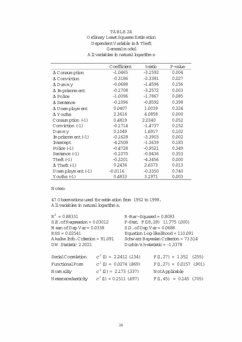
Forecasts from either of these short run models may be compared with theforecasts from a general (unrestricted) single equation error- correction model or a model resulting from a specification search. Tables 24 and 25 report the estimated general model for Theft and associated forecasts and Tables 26 and 27 those for the reduced model.
24
TABLE 24Ordinary Least Squares EstimationDependent Variable is ∆ Theft
General modelAll variables in natural logarithms
Coefficient t-ratio P-value∆ Consum ption -1.0465 -3.1592 0.004∆ Conviction -0.3186 -2.3381 0.027∆ Dummy -0.0688 -1.4596 0.156∆ Imprisonment -0.1708 -3.2572 0.003∆ Police -1.0096 -1.7867 0.085∆ Sentence -0.1096 -0.8592 0.398∆ Unemployment 0.0407 1.0039 0.324∆ Youths 2.3616 4.0858 0.000Consumption (-1) 0.4819 2.0340 0.052Conviction (-1) -0.1714 -1.4737 0.152Dummy 0.1049 1.6917 0.102Imprisonment (-1) -0.1628 -3.3903 0.002Intercept -4.2508 -1.3639 0.183Police (-1) -0.4728 -0.9521 0.349Sentence (-1) -0.1070 -0.9436 0.353Theft (-1) -0.3201 -4.3456 0.000∆ Theft (-1) 0.2436 2.6373 0.013Unemployment (-1) -0.0116 -0.3350 0.740Youths (-1) 0.4833 3.1971 0.003
Notes:
47 Observations used for estimation from 1952 to 1998. All variables in natural logarithms.
R2 = 0.88331 R-Bar–Squared = 0.8083S.E. of Regression = 0.03012 F-Stat. F(18, 28) 11.775 (.000)M ean of Dep Var = 0.0338 S.D. of Dep Var = 0.0688 RSS = 0.02541 Equation Log-likelihood = 110.091Akaike Info. Criterion = 91.091 Schwarz Bayesian Criterion = 73.514DW Statistic 2.3021 Durbin’s h-statistic = -1.3378
Serial Correlation )1(2c = 2.2412 (.134) F(1, 27) = 1.352 (.255)
Functional Form )1(2c = 0.0274 (.869) F(1, 27) = 0.0157 (.901)
Normality )2(2c = 2.173 (.337) Not Applicable
Heteroscedasticity )1(2c = 0.1511 (.697) F(1, 45) = 0.145 (.705)
25
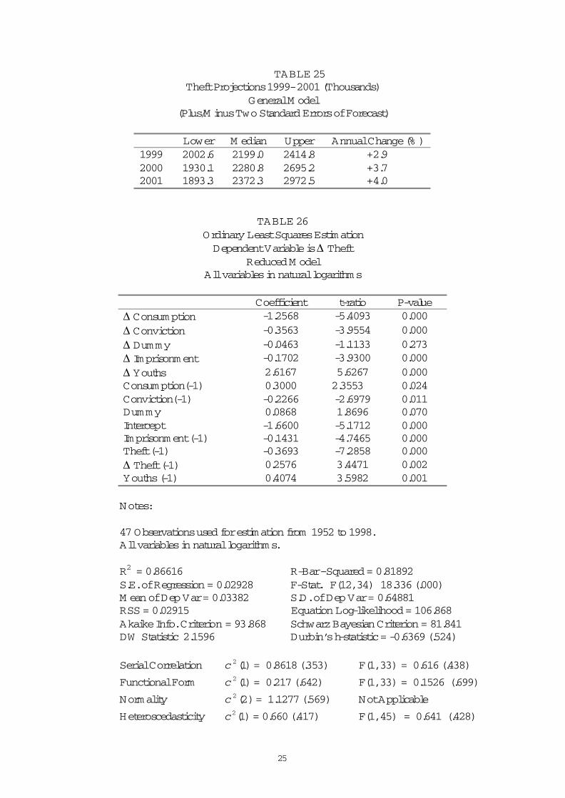
TABLE 25Theft Projections 1999- 2001 (Thousands)
General M odel(Plus/M inus Two Standard Errors of Forecast)
Lower M edian Upper Annual Change (% )1999 2002.6 2199.0 2414.8 +2.92000 1930.1 2280.8 2695.2 +3.72001 1893.3 2372.3 2972.5 +4.0
TABLE 26Ordinary Least Squares EstimationDependent Variable is ∆ Theft
Reduced M odelAll variables in natural logarithms
Coefficient t-ratio P-value∆ Consum ption -1.2568 -5.4093 0.000∆ Conviction -0.3563 -3.9554 0.000∆ Dummy -0.0463 -1.1133 0.273∆ Imprisonment -0.1702 -3.9300 0.000∆ Youths 2.6167 5.6267 0.000Consumption(-1) 0.3000 2.3553 0.024Conviction(-1) -0.2266 -2.6979 0.011Dummy 0.0868 1.8696 0.070Intercept -1.6600 -5.1712 0.000Imprisonment (-1) -0.1431 -4.7465 0.000Theft (-1) -0.3693 -7.2858 0.000∆ Theft (-1) 0.2576 3.4471 0.002Youths (-1) 0.4074 3.5982 0.001
Notes:
47 Observations used for estimation from 1952 to 1998. All variables in natural logarithms.
R2 = 0.86616 R-Bar–Squared = 0.81892S.E. of Regression = 0.02928 F-Stat. F(12, 34) 18.336 (.000)M ean of Dep Var = 0.03382 S.D. of Dep Var = 0.64881 RSS = 0.02915 Equation Log-likelihood = 106.868Akaike Info. Criterion = 93.868 Schwarz Bayesian Criterion = 81.841DW Statistic 2.1596 Durbin’s h-statistic = -0.6369 (.524)
Serial Correlation )1(2c = 0.8618 (.353) F(1, 33) = 0.616 (.438)
Functional Form )1(2c = 0.217 (.642) F(1, 33) = 0.1526 (.699)
Normality )2(2c = 1.1277 (.569) Not Applicable
Heteroscedasticity )1(2c = 0.660 (.417) F(1, 45) = 0.641 (.428)
26
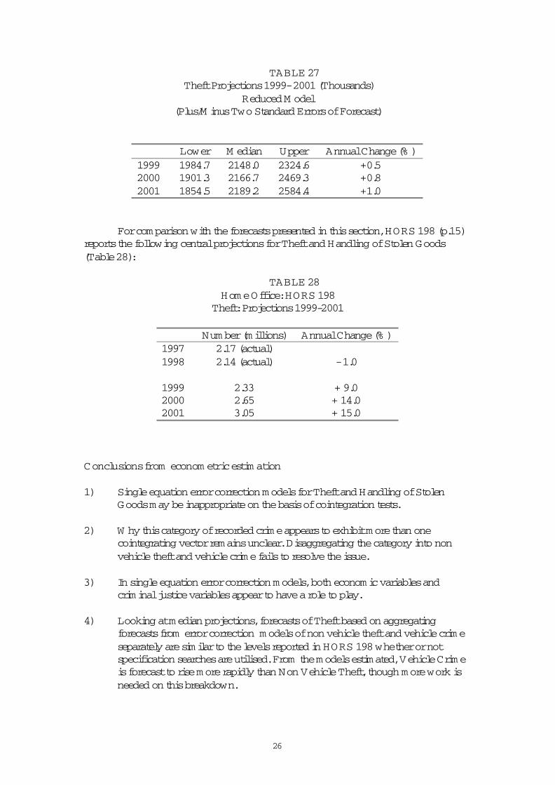
TABLE 27 Theft Projections 1999- 2001 (Thousands)
Reduced M odel(Plus/M inus Two Standard Errors of Forecast)
Lower M edian Upper Annual Change (% )1999 1984.7 2148.0 2324.6 +0.52000 1901.3 2166.7 2469.3 +0.82001 1854.5 2189.2 2584.4 +1.0
For comparison with the forecasts presented in this section, HORS 198 (p.15) reports the following central projections for Theft and Handling of Stolen Goods (Table 28):
TABLE 28Home Office: HORS 198
Theft: Projections 1999-2001
Number (millions) Annual Change (% )1997 2.17 (actual)1998 2.14 (actual) - 1.0
1999 2.33 + 9.02000 2.65 + 14.02001 3.05 + 15.0
Conclusions from econom etric estim ation
1) Single equation error correction models for Theft and Handling of Stolen Goods may be inappropriate on the basis of cointegration tests.
2) W hy this category of recorded crime appears to exhibit more than one cointegrating vector remains unclear. Disaggregating the category into non vehicle theft and vehicle crime fails to resolve the issue.
3) In single equation error correction models, both economic variables and criminal justice variables appear to have a role to play.
4) Looking at median projections, forecasts of Theft based on aggregating forecasts from error correction models of non vehicle theft and vehicle crime separately are similar to the levels reported in HORS 198 whether or not specification searches are utilised. From the models estimated, Vehicle Crime is forecast to rise more rapidly than Non Vehicle Theft, though more work is needed on this breakdown.
27
5) Econometric error correction models of Theft based on aggregate data directly produce median forecasts well below those in HORS 198.
6) Short Run models which exclude error correction terms generally give rise to lower forecast values than models which include such terms.
7) No models gave rise to forecast values as large as those in HORS 198 by the end of the forecast period.
8) All models produce standard errors of forecast which imply a large range of uncertainty for the forecast values
Time Series M odelling
One would not expect traditional time-series forecasting models, such as Box-Jenkinsmodels, to replicate the above predicted patterns for recorded crime given the assumptions made about the future state of the economy (consumption and unemployment) and the relatively small forecast increase in the number of males aged 15 to 24 over the forecast period. Stationary univariate Box-Jenkins (ARIM A) models produce optimal (minimum mean squared error) forecasts that revert quickly to the mean of the process, which are therefore only intended for short run forecasts.However, such models are useful for obtaining an initial specification of the noise component of multivariate transfer function models which allow for the influence of independent variables and hence are available for longer run forecasting.
The autocorrelation function (acf) of the log of Burglary shows a clearly nonstationary series and the time series plot reveals the structural (recording) break in 1968. Although the break is less evident in the Theft series, it is still the case that this series may have been affected by the change in recording practice following the Theft Act of 1968. Deadman (2000) has shown that the identification of time series models for Residential Burglary was more straightforward if the series used had been adjusted for the effects of the Theft Act prior to analysis. Accordingly, in the identification stages of time series modelling below, the series for Burglary and Theft used in HORS 198 were utilised. However, the estimation of the final models selected and the forecasting from these models was done using the original (unadjusted) series together with a dummy variable to allow for the break (and is therefore consistent with the econometric results above). All time series models were centered before estimation.
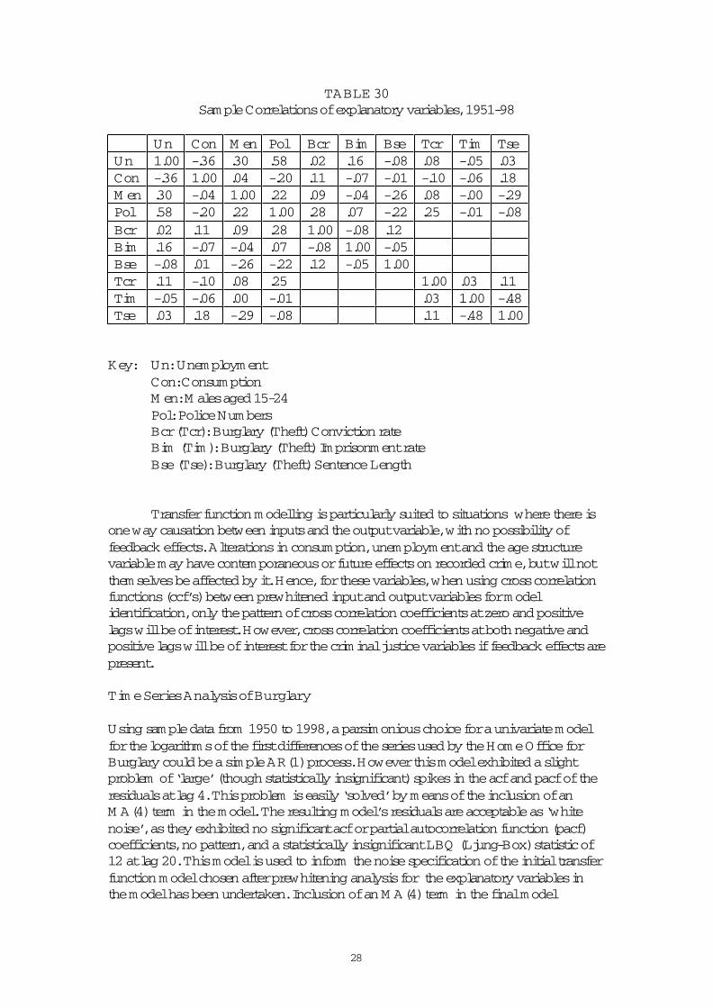
Following the methodology first proposed by Box and Jenkins (1970) (see also M cLeod (1982) and Vandaele (1983)), separate univariate models were built for each of the independent variables. These were used for prewhitening the output variable in the identification stage of modelling in a ‘piece-meal’ fashion to specify the complete transfer function model. This approach may be expected to work quite well in the multiple input case provided the independent variables are only weakly related (see M ills (1990, p.261). As each variable is differenced for stationarity, this requirement is generally met, as may be seen from the sample correlations of the differences of the natural logarithms of the variables in Table 30:
28
TABLE 30Sample Correlations of explanatory variables, 1951-98
Un Con M en Pol Bcr Bim Bse Tcr Tim TseUn 1.00 -.36 .30 .58 .02 .16 -.08 .08 -.05 .03Con -.36 1.00 .04 -.20 .11 -.07 -.01 -.10 -.06 .18M en .30 -.04 1.00 .22 .09 -.04 -.26 .08 -.00 -.29Pol .58 -.20 .22 1.00 .28 .07 -.22 .25 -.01 -.08Bcr .02 .11 .09 .28 1.00 -.08 .12Bim .16 -.07 -.04 .07 -.08 1.00 -.05Bse -.08 .01 -.26 -.22 .12 -.05 1.00Tcr .11 -.10 .08 .25 1.00 .03 .11Tim -.05 -.06 .00 -.01 .03 1.00 -.48Tse .03 .18 -.29 -.08 .11 -.48 1.00
Key: Un: UnemploymentCon: Consum ptionM en: M ales aged 15-24Pol: Police NumbersBcr (Tcr): Burglary (Theft) Conviction rateBim (Tim): Burglary (Theft) Imprisonment rateBse (Tse): Burglary (Theft) Sentence Length
Transfer function modelling is particularly suited to situations where there is one way causation between inputs and the output variable, with no possibility of feedback effects. Alterations in consumption, unemployment and the age structure variable may have contemporaneous or future effects on recorded crime, but will not themselves be affected by it. Hence, for these variables, when using cross correlation functions (ccf’s) between prewhitened input and output variables for model identification, only the pattern of cross correlation coefficients at zero and positive lags will be of interest. However, cross correlation coefficients at both negative and positive lags will be of interest for the criminal justice variables if feedback effects are present.
Tim e Series Analysis of Burglary
Using sample data from 1950 to 1998, a parsimonious choice for a univariate model for the logarithms of the first differences of the series used by the Home Office for Burglary could be a simple AR(1) process. However this model exhibited a slight problem of ‘large’ (though statistically insignificant) spikes in the acf and pacf of the residuals at lag 4. This problem is easily ‘solved’ by means of the inclusion of an M A(4) term in the model. The resulting model’s residuals are acceptable as ‘white noise’, as they exhibited no significant acf or partial autocorrelation function (pacf) coefficients, no pattern, and a statistically insignificant LBQ (Ljung-Box) statistic of 12 at lag 20. This model is used to inform the noise specification of the initial transfer function model chosen after prewhitening analysis for the explanatory variables in the model has been undertaken. Inclusion of an M A(4) term in the final model
29
specification left forecast values virtually unchanged compared with models which excluded this term however.
Univariate models were constructed and estimated for the logarithms of the first differences of each of the economic, demographic and criminal justice variables used in the earlier econometric analysis. These models were used in turn to filter the logarithms of the first differences of the Home Office Burglary series to identify (clarify) the dynamics between the explanatory variables and Burglary. Unemployment and the Youths variable were modelled by AR(2) processes, and Consumption by an AR(1) process. The appropriate model for Police was less clear, and a number of autoregressive alternatives were adopted. An AR(2) model for the conviction rate was possibly indicated, but no convincing models for either the probability of imprisonment or sentence length suggested themselves. ‘Best’ models appeared to be an AR(1) model for the former and a statistically sound but unconvincing M A(5) model for the latter. The lack of convincing univariate models for the criminal justice variables does not rule out their appearance in a model to explain Burglary as these models are only used to provide an initial view of model specification. Subsequent modelling may well alter the initial views about the form and impact (if any) of any of the explanatory variables investigated at this stage.
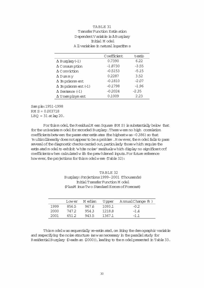
The adopted univariate models were used to prewhiten the Burglary series used in HORS 198 and the cross correlation functions (ccfs) between the prewhitened inputs and outputs calculated. For the unemployment variable there were significant positive ccf coefficients at lags –1 and 0. Unless recorded crime rises are a leading indicator for unemployment, only the contemporaneous effect is of interest for the transfer modelling. For consumption, there is a marked contemporaneous effect indicated, with other ‘large’ but not significant coefficients at low positive lags. This suggests that the effects of this variable may be spread out over time. The only significant ccf coefficient for the demographic variable is an unconvincing negative coefficient at lag 2. There were no significant ccf coefficients for the police variable which is omitted from the transfer function modelling. The conviction rate exhibited a significant negative ccf coefficient at lag 0, a result that was constant across a variety of models used for this variable in the prewhitening exercise. The ccf for the probability of imprisonment suggested effects at lags 0 and 1, and the sentence length ccf suggested a one period lag for the initial model. W ith these implied effects together with an initial AR(1) noise process suggested by the univariate model for recorded Burglary, the initial transfer model was estimated and is given in Table 31.
30
TABLE 31Transfer Function Estimation
Dependent Variable is ∆BurglaryInitial M odel
All variables in natural logarithms
Coefficient t-ratio∆ Burglary(-1) 0.7390 6.22∆ Consum ption -1.8730 -3.55∆ Conviction -0.5153 -5.15∆ Dummy 0.2287 3.52∆ Imprisonment -0.1810 -2.07∆ Imprisonment (-1) -0.1798 -1.96∆ Sentence (-1) -0.2024 -2.35∆ Unemployment 0.1009 2.23
Sample: 1951-1998RM S = 0.003718LBQ = 31 at lag 20.
For this model, the Residual M ean Square (RM S) is substantially below that for the univariate model for recorded Burglary. There were no high correlation coefficients between the parameter estimates (the highest was –0.386) so that ‘multicollinearity does not appear to be a problem. However, the model fails to pass several of the diagnostic checks carried out, particularly those which require the estimated model to exhibit ‘white noise’ residuals which display no significant ccf coefficients when calculated with the prewhitened inputs. For future reference however, the projections for this model were (Table 32):
TABLE 32 Burglary: Projections 1999- 2001 (Thousands)
Initial Transfer Function M odel(Plus/M inus Two Standard Errors of Forecast)
Lower M edian Upper Annual Change (% )1999 856.5 967.6 1093.1 -0.22000 747.2 954.3 1218.8 -1.42001 651.2 943.5 1367.1 -1.1
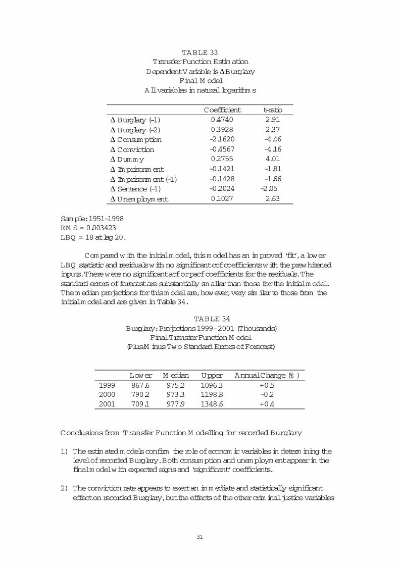
This model was sequentially re-estimated, omitting the demographic variable and respecifying the noise structure (as was necessary in the parallel study for Residential Burglary (Deadman (2000)), leading to the model presented in Table 33.
31
TABLE 33Transfer Function Estimation
Dependent Variable is ∆BurglaryFinal M odel
All variables in natural logarithms
Coefficient t-ratio∆ Burglary (-1) 0.4740 2.91∆ Burglary (-2) 0.3928 2.37∆ Consum ption -2.1620 -4.46∆ Conviction -0.4567 -4.16∆ Dummy 0.2755 4.01∆ Imprisonment -0.1421 -1.81∆ Imprisonment (-1) -0.1428 -1.66∆ Sentence (-1) -0.2024 -2.05∆ Unemployment 0.1027 2.63
Sample: 1951-1998RM S = 0.003423LBQ = 18 at lag 20.
Compared with the initial model, this model has an improved ‘fit’, a lower LBQ statistic and residuals with no significant ccf coefficients with the prewhitened inputs. There were no significant acf or pacf coefficients for the residuals. The standard errors of forecast are substantially smaller than those for the initial model. The median projections for this model are, however, very similar to those from the initial model and are given in Table 34.
TABLE 34 Burglary: Projections 1999- 2001 (Thousands)
Final Transfer Function M odel(Plus/M inus Two Standard Errors of Forecast)
Lower M edian Upper Annual Change (% )1999 867.6 975.2 1096.3 +0.52000 790.2 973.3 1198.8 -0.22001 709.1 977.9 1348.6 +0.4
Conclusions from Transfer Function M odelling for recorded Burglary
1) The estimated models confirm the role of economic variables in determining the level of recorded Burglary. Both consumption and unemployment appear in the final model with expected signs and ‘significant’ coefficients.
2) The conviction rate appears to exert an immediate and statistically significant effect on recorded Burglary, but the effects of the other criminal justice variables
32
in the model (sentence length and the probability of imprisonment) are less well determined.
3) The time series modelling exercise results in a final model not too dissimilar to the short run econometric model reported earlier (Table 6) and, therefore, produces forecasts in line with that model.
4) Using predicted values for consumption and unemployment for the forecast period which are not far removed from those existing at the end of the sample period, the time series model predicts median values of recorded Burglary which are little changed to 2001.
Tim e Series Analysis of Recorded Theft and Handling of Stolen Goods
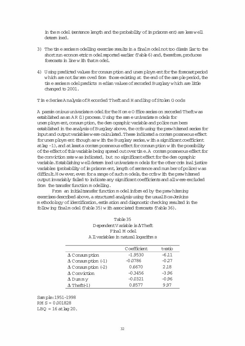
A parsimonious univariate model for the Home Office series on recorded Theft was established as an AR(1) process. Using the same univariate models for unemployment, consumption, the demographic variable and police numbers established in the analysis of Burglary above, the ccfs using the prewhitened series for input and output variables were calculated. These indicated a contemporaneous effect for unemployment (though as with the Burglary series, with a significant coefficient at lag –1), and at least a contemporaneous effect for consumption with the possibility of the effect of this variable being spread out over time. A contemporaneous effect for the conviction rate was indicated, but no significant effect for the demographic variable. Establishing well determined univariate models for the other criminal justice variables (probability of imprisonment, length of sentence and number of police) was difficult. However, even for a range of such models, the ccfs with the prewhitened output invariably failed to indicate any significant coefficients and all were excluded from the transfer function modelling.
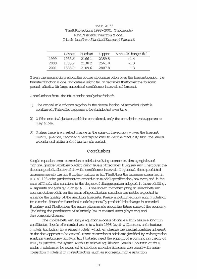
From an initial transfer function model informed by the prewhitening exercises described above, a structured analysis using the usual Box-Jenkinsmethodology of identification, estimation and diagnostic checking resulted in the following final model (Table 35) with associated forecasts (Table 36).
Table 35Dependent Variable is ∆Theft
Final M odelAll variables in natural logarithms
Coefficient t-ratio∆ Consum ption -1.9530 -6.11∆ Consumption (-1) -0.0786 -0.27∆ Consumption (-2) 0.6670 2.18∆ Conviction -0.3456 -3.96∆ Dummy -0.0321 -0.96∆ Theft(-1) 0.8577 9.97
Sample: 1951-1998RM S = 0.001828LBQ = 16 at lag 20.
33
TABLE 36 Theft Projections 1998- 2001 (Thousands)
Final Transfer Function M odel(Plus/M inus Two Standard Errors of Forecast)
Lower M edian Upper Annual Change (% )1999 1988.6 2166.1 2359.5 +1.42000 1785.2 2138.2 2561.0 -1.32001 1585.0 2109.6 2807.8 -1.3
Given the assumptions about the course of consumption over the forecast period, the transfer function model indicates a slight fall in recorded theft over the forecast period, albeit with large associated confidence intervals of forecast.
Conclusions from the tim e series analysis of Theft
1) The central role of consumption in the determination of recorded Theft is confirm ed. This effect appears to be distributed over time.
2) Of the criminal justice variables considered, only the conviction rate appears to play a role.
3) Unless there is a marked change in the state of the economy over the forecast period, (median) recorded Theft is predicted to decline gradually from the levels experienced at the end of the sample period.
Conclusions
Single equation error-correction models involving economic, demographic and criminal justice variables predict rising levels of recorded Burglary and Theft over the forecast period, albeit within wide confidence intervals. In general, these predicted increases are similar for Burglary but lower for Theft than the increases presented in HORS 198. The predictions are sensitive to model specification, however, and in the case of Theft, also sensitive to the degree of disaggregation adopted in the modelling. A separate analysis by Pudney (2000) has shown that attempting to select between econometric models on the basis of specification searches can not be expected to enhance the quality of the resulting forecasts. Purely short run econometric models or time series (Transfer Function) models generally predict little change in recorded Burglary and Theft given the assumptions made about the future state of the economy (including the persistence of relatively low measured unemployment) and demographic change.
The choice between single equation models of crime which assume long run equilibrium levels of recorded crime to which 1998 levels will return, and short run models (including time series models) which emphasise the inertial qualities inherent in the data appears to be crucial. Error-correction models are justified by cointegration analysis (particulary for Burglary) but also need the support of a convincing theory of how, in practice, the system works to restore equilibrium levels. Short run or time series models may be expected to produce superior forecasts compared with error-correction models if important factors (such as successful crime reduction

34
programmes) are omitted from the analysis, or if the relationships are subject to structural changes. The actual path of recorded Burglary and Theft to 2001 from the levels experienced in 1998 will be highly suggestive as to the utility of these two types of model for crime forecasting.
35
DATA APPENDIX
Definitions of Variables and Sources of Data
Burglary (BURGPC): Number of recorded offences of Burglary (Categories 28 to31) per capita in England and W ales. Criminal Statistics.
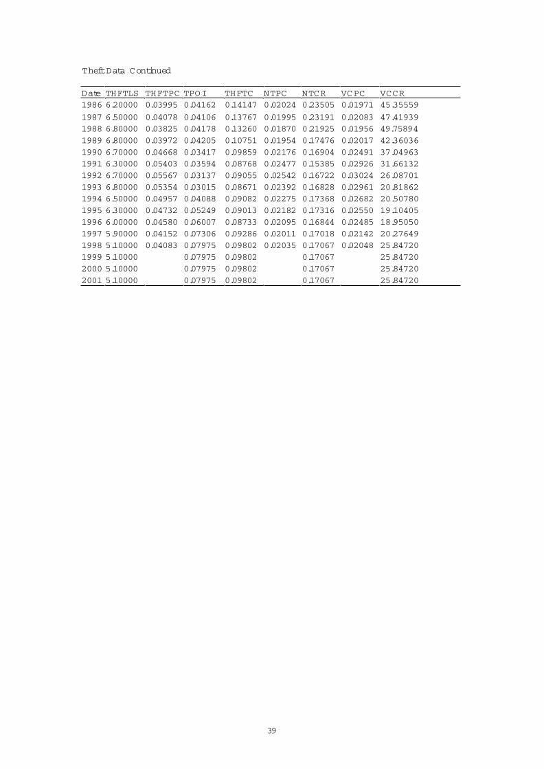
Theft (THFTPC): Number of recorded offences of Theft and Handling of Stolen Goods (Categories 37, 39-49 and 54) per capita in England and W ales. Criminal Statistics.
Vehicle Crim e (VCPC): Number of recorded offences of theft from a vehicle and theft of a vehicle (categories 45 and 48) per capita in England and W ales: Criminal Statistics.
Vehicle Crim e Conviction Rate (VCCR): Vehicle Crime Convictions divided by number of recorded offences of Vehicle Crime (x1000).
Non Vehicle Theft (NTPC): Theft minus Vehicle Crime per capita in England and W ales.
Non Vehicle Theft Conviction Rate (NTCR): Non Vehicle Theft Convictions divided by number of recorded Non Vehicle Thefts.
Unem ploym ent (UNEM ): Number registered as unemployed in the UK excluding adult students per capita. Economic Trends
Consum ption (CONS): Total UK Household Final Consumption Expenditure per capita at 1995 prices. Economic Trends.
Conviction Rate (BURGC and THFTC): Number of convictions for burglary (theft) in England and W ales divided by the number of recorded burglaries (theft). Criminal Statistics.
Sentence Length (BURGLS and THFTLS): Average length (months) of prison sentence for burglary (theft) convictions. Criminal Statistics and unpublished data provided by the Home Office.
Prison (BPOI and TPOI): Number imprisoned for burglary (theft) divided by number convicted for burglary (theft). Criminal Statistics.
Police (POL): End of Year Strength (excluding special constables). England and W ales. Annual Abstract of Statistics.
Youths (YOUTH): Number of males aged 15-24 years as a proportion of population of England and W ales. Population Trends.
Dum m y (D): Theft Act (1968) dummy. D = 0 for t = 1950 - 68. D = 1 for t > 1968
36
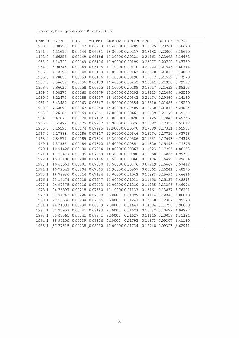
Econom ic, Dem ographic and Burglary Data
Date D UNEM POL YO UTH BURG LS BURG PC BPOI BURGC CO NS1950 0 5.88750 0.00142 0.06733 16.40000 0.00209 0.18325 0.20761 3.38670
1951 0 4.11610 0.00144 0.06281 18.80000 0.00217 0.18182 0.22000 3.356101952 0 6.66257 0.00149 0.06186 17.30000 0.00221 0.21963 0.22062 3.344721953 0 6.14722 0.00149 0.06196 17.90000 0.00199 0.23077 0.20729 3.477591954 0 5.00345 0.00149 0.06135 17.10000 0.00170 0.22222 0.21543 3.607441955 0 4.12193 0.00148 0.06159 17.00000 0.00167 0.20370 0.21833 3.740801956 0 4.20053 0.00153 0.06116 17.10000 0.00190 0.19672 0.21529 3.739701957 0 5.36652 0.00156 0.06139 16.60000 0.00232 0.18341 0.21998 3.795271958 0 7.86030 0.00158 0.06225 16.10000 0.00288 0.19217 0.21632 3.883531959 0 8.08376 0.00160 0.06379 15.30000 0.00292 0.19113 0.22080 4.025401960 0 6.22470 0.00158 0.06497 15.40000 0.00343 0.21474 0.19860 4.141691961 0 5.43489 0.00163 0.06667 14.50000 0.00354 0.18310 0.21686 4.192201962 0 7.62098 0.00167 0.06940 14.20000 0.00409 0.18750 0.21814 4.240241963 0 9.26185 0.00169 0.07081 12.00000 0.00462 0.16739 0.21179 4.391971964 0 6.47676 0.00170 0.07172 11.80000 0.00490 0.16425 0.17845 4.493361965 0 5.51477 0.00175 0.07227 11.90000 0.00526 0.16782 0.17358 4.510121966 0 5.15596 0.00174 0.07295 12.90000 0.00570 0.17089 0.17331 4.559631967 0 9.17883 0.00186 0.07317 12.90000 0.00546 0.16274 0.17710 4.637281968 0 9.84577 0.00185 0.07324 15.30000 0.00586 0.11531 0.17693 4.743981969 1 9.37336 0.00184 0.07302 13.60000 0.00851 0.11820 0.15498 4.743751970 1 10.01426 0.00190 0.07294 14.00000 0.00867 0.11323 0.17296 4.862631971 1 13.50477 0.00195 0.07269 14.30000 0.00900 0.10858 0.16866 4.993271972 1 15.00188 0.00200 0.07106 15.50000 0.00868 0.10496 0.16472 5.296841973 1 10.65561 0.00201 0.07050 10.50000 0.00776 0.09219 0.16667 5.574421974 1 10.72041 0.00204 0.07065 11.90000 0.00957 0.08062 0.16241 5.482901975 1 16.73930 0.00214 0.07134 12.00000 0.01042 0.10383 0.15694 5.466361976 1 23.16479 0.00218 0.07277 11.00000 0.01031 0.11658 0.15137 5.488931977 1 24.97375 0.00216 0.07423 11.00000 0.01210 0.11985 0.13386 5.469941978 1 24.76897 0.00218 0.07550 11.10000 0.01133 0.13161 0.13837 5.762211979 1 23.04943 0.00226 0.07698 8.70000 0.01099 0.14114 0.12240 6.008181980 1 29.56636 0.00234 0.07905 8.20000 0.01247 0.13838 0.12387 5.992701981 1 44.71891 0.00238 0.08079 7.80000 0.01447 0.14994 0.11790 5.988581982 1 51.77953 0.00241 0.08193 7.70000 0.01623 0.16232 0.10479 6.042971983 1 55.07565 0.00241 0.08271 8.60000 0.01627 0.14145 0.10058 6.313241984 1 55.94109 0.00239 0.08306 9.40000 0.01793 0.11673 0.09307 6.411501985 1 57.77315 0.00238 0.08292 10.00000 0.01734 0.12748 0.09323 6.62941
37
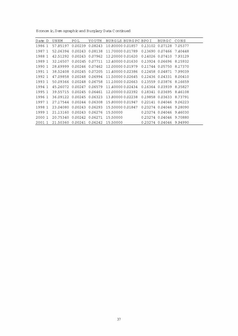
Econom ic, Dem ographic and Burglary Data Continued
Date D UNEM POL YO UTH BURG LS BURG PC BPOI BURGC CONS1986 1 57.85197 0.00239 0.08243 10.80000 0.01857 0.13102 0.07128 7.05377
1987 1 52.06394 0.00243 0.08138 11.70000 0.01789 0.13690 0.07466 7.404481988 1 42.51292 0.00243 0.07962 12.20000 0.01620 0.14026 0.07410 7.931291989 1 32.16507 0.00245 0.07711 12.40000 0.01630 0.13924 0.06696 8.159321990 1 28.69999 0.00246 0.07462 12.00000 0.01979 0.11744 0.05750 8.173701991 1 38.52408 0.00245 0.07205 11.40000 0.02386 0.12458 0.04871 7.990391992 1 47.09858 0.00248 0.06994 11.50000 0.02645 0.12436 0.04331 8.004101993 1 50.09366 0.00248 0.06758 11.10000 0.02663 0.13559 0.03876 8.166591994 1 45.26072 0.00247 0.06579 11.40000 0.02434 0.16364 0.03939 8.358271995 1 39.55715 0.00245 0.06461 12.00000 0.02392 0.18341 0.03695 8.461081996 1 36.09122 0.00245 0.06323 13.80000 0.02238 0.19858 0.03633 8.737911997 1 27.17544 0.00244 0.06308 15.80000 0.01947 0.22141 0.04046 9.062231998 1 23.04080 0.00243 0.06293 15.50000 0.01847 0.23274 0.04046 9.280901999 1 21.13160 0.00243 0.06276 15.50000 0.23274 0.04046 9.460302000 1 20.75340 0.00242 0.06271 15.50000 0.23274 0.04046 9.708802001 1 21.50360 0.00241 0.06242 15.50000 0.23274 0.04046 9.94990
38
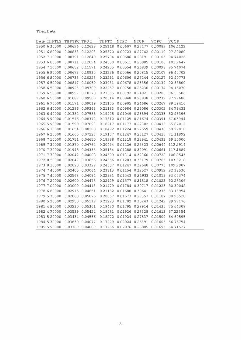
Theft Data
Date THFTLS THFTPC TPO I THFTC NTPC NTCR VCPC VCCR1950 6.30000 0.00696 0.12629 0.25318 0.00607 0.27477 0.00089 106.4122
1951 6.80000 0.00833 0.12203 0.25370 0.00723 0.27742 0.00110 97.800801952 7.10000 0.00791 0.12640 0.25704 0.00686 0.28191 0.00105 94.740261953 6.80000 0.00711 0.12094 0.24530 0.00611 0.26885 0.00100 101.76471954 7.10000 0.00652 0.11571 0.24255 0.00554 0.26839 0.00098 95.740741955 6.90000 0.00673 0.10935 0.23236 0.00566 0.25815 0.00107 96.457021956 6.80000 0.00733 0.10223 0.23291 0.00606 0.26244 0.00127 92.407731957 6.50000 0.00817 0.10059 0.23031 0.00678 0.25856 0.00139 92.688001958 6.50000 0.00923 0.09709 0.22257 0.00750 0.25230 0.00174 94.150701959 6.50000 0.00997 0.10178 0.21065 0.00792 0.24021 0.00205 96.595061960 6.50000 0.01087 0.09500 0.20514 0.00848 0.23838 0.00239 87.296801961 6.70000 0.01171 0.09019 0.21105 0.00905 0.24686 0.00267 89.594161962 6.40000 0.01286 0.09363 0.21183 0.00984 0.25086 0.00302 84.794331963 6.40000 0.01382 0.07585 0.19908 0.01049 0.23594 0.00333 82.953961964 5.90000 0.01516 0.08372 0.17812 0.01125 0.21674 0.00391 67.039441965 5.90000 0.01590 0.07893 0.18217 0.01177 0.22302 0.00413 65.870121966 6.10000 0.01654 0.08180 0.18492 0.01224 0.22559 0.00430 69.278101967 6.20000 0.01665 0.07227 0.19107 0.01247 0.23127 0.00418 71.119921968 7.10000 0.01751 0.04650 0.18988 0.01318 0.22941 0.00433 69.500001969 7.30000 0.01870 0.04764 0.20494 0.01226 0.25323 0.00644 112.99141970 7.70000 0.01948 0.04335 0.25184 0.01288 0.32091 0.00661 117.18891971 7.70000 0.02042 0.04008 0.24609 0.01314 0.32360 0.00728 106.05431972 8.50000 0.02047 0.03656 0.24656 0.01283 0.33179 0.00763 103.32181973 8.10000 0.02020 0.03329 0.24357 0.01247 0.32648 0.00773 109.79071974 7.40000 0.02405 0.03064 0.23313 0.01454 0.32527 0.00952 92.385301975 7.40000 0.02563 0.04094 0.22931 0.01543 0.31933 0.01019 93.053741976 7.20000 0.02600 0.04478 0.22929 0.01577 0.31818 0.01023 92.283061977 7.00000 0.03009 0.04413 0.21479 0.01784 0.30717 0.01225 80.300481978 6.80000 0.02915 0.04651 0.21182 0.01680 0.30641 0.01235 83.139541979 5.70000 0.02860 0.05076 0.20867 0.01673 0.29357 0.01187 88.965281980 5.20000 0.02950 0.05119 0.21223 0.01702 0.30243 0.01249 89.271761981 4.80000 0.03230 0.05361 0.19430 0.01795 0.28914 0.01435 75.643081982 4.70000 0.03539 0.05424 0.18481 0.01926 0.28328 0.01613 67.223541983 5.20000 0.03434 0.04556 0.18272 0.01924 0.27537 0.01509 64.605951984 5.70000 0.03630 0.04077 0.17229 0.02024 0.26391 0.01606 56.767541985 5.90000 0.03769 0.04089 0.17266 0.02076 0.26885 0.01693 54.71527
39
Theft Data Continued
Date THFTLS THFTPC TPOI THFTC NTPC NTCR VCPC VCCR1986 6.20000 0.03995 0.04162 0.14147 0.02024 0.23505 0.01971 45.35559
1987 6.50000 0.04078 0.04106 0.13767 0.01995 0.23191 0.02083 47.419391988 6.80000 0.03825 0.04178 0.13260 0.01870 0.21925 0.01956 49.758941989 6.80000 0.03972 0.04205 0.10751 0.01954 0.17476 0.02017 42.360361990 6.70000 0.04668 0.03417 0.09859 0.02176 0.16904 0.02491 37.049631991 6.30000 0.05403 0.03594 0.08768 0.02477 0.15385 0.02926 31.661321992 6.70000 0.05567 0.03137 0.09055 0.02542 0.16722 0.03024 26.087011993 6.80000 0.05354 0.03015 0.08671 0.02392 0.16828 0.02961 20.818621994 6.50000 0.04957 0.04088 0.09082 0.02275 0.17368 0.02682 20.507801995 6.30000 0.04732 0.05249 0.09013 0.02182 0.17316 0.02550 19.104051996 6.00000 0.04580 0.06007 0.08733 0.02095 0.16844 0.02485 18.950501997 5.90000 0.04152 0.07306 0.09286 0.02011 0.17018 0.02142 20.276491998 5.10000 0.04083 0.07975 0.09802 0.02035 0.17067 0.02048 25.847201999 5.10000 0.07975 0.09802 0.17067 25.847202000 5.10000 0.07975 0.09802 0.17067 25.847202001 5.10000 0.07975 0.09802 0.17067 25.84720

40
References
Box, G.E.P. and G.M .Jenkins (1970), Time Series Analysis; Forecasting and Control, Holden-Day, San Francisco.
Charemza, W .W . and D.F.Deadman (1997), New Directions in Econometric Practice,Second Edition, Edward Elgar, Cheltenham.
Darnell, A.C. (1994),A Dictionary of Econometrics, Edward Elgar, Cheltenham.
Deadman, D.F. (2000), ‘Forecasting Residential Burglary’, PSERC Discussion Paper No 00/6, University of Leicester, 19pp.
Deadman, D. and D.Pyle (1997), ‘Forecasting Recorded Property Crime Using a Time-Series Econometric M odel’, British Journal of Criminology, Vol 37, No. 3, pp 437-445.
Dhiri, S., S.Brand, R.Harries and R.Price (1999),M odelling and Predicting Property Crime Trends, Home Office Research Study 198, London, HM SO.
Field, S.(1990), Trends in Crime and their Interpretation: A Study of Recorded Crime in Post-war England and W ales’, Home Office Research Study 118, London, HM SO.
Field, S. (1999), Trends in Crime Revisited, Home Office Research Study 195, London, HM SO.
GAD (1999). National Population Projections. Government Actuary’s Department. Office for National Statistics. Series PP2. No.21.
Hale, C. (1998), ‘Crime and the Business Cycle in Post-W ar Britain Revisited’, British Journal of Criminology’, Vol. 38, No. 4, pp. 681-698.
Hale, C. and D.Sabbagh (1991), ‘Testing the Relationship between Unemployment and Crime: A M ethodological Comment and Empirical Analysis using Time-SeriesData for England and W ales’, Journal of Research in Crime and Delinquency, Vol 28, pp 400-17.
HM T (1999). Budget 99. H.M . Treasury. M arch. H.M .S.O. London.
M acdonald, Z. and D.J.Pyle (eds.) (2000), The Economics of Illicit Activity, Ashgate.
M cLeod, G. (1983), Box Jenkins in Practice, Gwilym Jenkins & Partners Ltd, Lancaster.
M ills, T.C. (1990), Time Series Techniques for Economists, Cambridge University Press, Cambridge.
NIESR (1999), National Institute Economic Review, No.4.

41
Pesaran, M .H. and B. Pesaran (1997), W orking with M icrofit 4.0 Interactive Econometric Analysis, Oxford University Press, Oxford.
Pudney, S.E. (2000), ‘Specification Search, Pretesting and the Precision of Dynamic Regression Forecasts: An Application to an Econometric M odel of Crime’, M imeo,University of Leicester, 29pp.
Pudney, S., D.Deadman and D.Pyle (1997), ‘The Effect of Under-Reporting in Statistical M odels of Criminal Activity: Estimation of an Error Correction M odel with M easurement Error’, Discussion Papers in Public Sector Economics No. 97/3, University of Leicester.
Pudney, S., D.Deadman and D.Pyle (2000), ‘The Relationship between Crime, Punishment and Economic Conditions: Is Reliable Inference Possible when Crimes are Under-Recorded?’, Journal of the Royal Statistical Society; Series A, Vol. 163, pp.81-97.
Pyle, D.J. and D.F.Deadman (1994), ‘Crime and the Business Cycle in Post-W arBritain’,British Journal of Criminology, Vol. 34, No. 3, pp 339-357.
Scorcu, A.E. and R.Cellini (1998), ‘Economic Activity and Crime in the Long Run: An Empirical Investigation on Aggregate Data from Italy, 1951-1994’,InternationalReview of Law and Economics, Vol. 18, No. 3, pp. 279-292.
Vandaele, W . (1983), Applied Time Series and Box-Jenkins M odels, Academic Press, Orlando, Florida.