FORECASTING RESERVOIR WATER LEVEL BASED ON THE …stmlportal.net/2ndCTOM/index.php/eProc181122/pdf/p372.pdf · Email: [email protected] ABSTRACT Reservoir water level is

Proceedings of the 2nd Conference on Technology & Operations Management (2ndCTOM)

Universiti Utara Malaysia, Kedah, Malaysia, February 26-27, 2018

372

FORECASTING RESERVOIR WATER LEVEL BASED ON THE CHANGE IN

RAINFALL PATTERN USING NEURAL NETWORK

Raja Nurul Mardhiah Raja Mohamad, W.H.W. Ishak

School of Information Technology, Universiti UtaraMalaysia, 06010 Sintok, Kedah,

MALAYSIA

Email: [email protected]

ABSTRACT

Reservoir water level is a level of storage space for water. During heavy rainfall, water

storage space is used to hold excessive amount of water. During less rainfall, water

storage maintains the water supply for its major uses. The change in rainfall pattern may

influence the water storage. Thus, understanding the change in rainfall pattern can be

used in gate opening decision. On top of that, the upstream precipitation is always not

coincide with the consequences and the flood downstream usually cause expensive

damages and great devastation as well. This study focus on the analysis of the upstream

rainfall data in order to obtain the rainfall pattern. This study deployed basic steps in

Artificial Neural Network (ANN) modeling which are data selection, data preparation,

data pre-processing and finally Neural Network model development and evaluation. The

performance of ANN was based on MAE (mean absolute error) and RMSE (root mean

square error). In this study, three datasets have been formed that represent the change in

upstream rainfall pattern. The findings show that the best RMSE achieve is 0.644 from

the third dataset.

Keywords: reservoir water level, rainfall pattern, artificial neural network.

INTRODUCTION

Decision on the amount of water to be stored and released is a tough task (Wurbs, 1993).

This is because the water discharge or the gate opening decision relies upon the standard

operation procedure (SOP). SOP is defined as an arrangement of well-ordered directions

accumulated by an association to enable laborers to do complex routine operations. Once

the water storage level increment up to the most extreme level, the water is discharged

that is the gate is opened.

To maintain a strategic distance from surge downstream, early water release is required

(Ishak, et al., 2011). Early water release relies upon the upstream precipitation. Along

these lines, the water storage level can be determined, early water discharge can be

executed. Existing study used precipitation size (total or average) to gauge and conjecture

store water level. In any case, the information does not reveal the actual pattern of



373

precipitation. Along these lines, in this study the change in upstream precipitation pattern

is investigated. The anticipating model that use neural network is created.

This study is aimed to analyze the upstream rainfall data in order to obtain the rainfall

pattern. Other than that, forecasting model is developed using neural network to learn the

rainfall pattern. Lastly the performance of neural network model is evaluated based on

the average.of samples (Nash et al., 1970) and RMSE.

The reservoir water level forecasting model is useful in supporting the reservoir operator

decision making. The change in upstream rainfall pattern provides some insight on

incoming inflow. This is important to avoid flood risk and eventually, minimize the

flood damage.

RELATED WORK

With the computational assets accessible today to most modelers, it has turned out to be

doable to assemble and apply very complex appropriated hydrological models that speak

to numerous distinctive procedures and comprise of many model components. Among the

first to perceive, be that as it may, that, in hydrology, ''better'' isn't really ''better'' were

(Stephenson et al., 1972) and there is a long reputation of studies showing and talking

about the troubles in display recognizable proof and alignment once the model turns out

to be excessively intricate (e.g., (Loague et al., 1985), (Beaven, 1985), (Blo¨schl, 2005)).

What is the purpose behind this outlandish reality, which is evidently at fluctuation with

involvement in liquid flow and different geosciences? There now is a developing

mindfulness that appropriated hydrological models are not the same as models in sister

teaches in no less than three imperative perspectives. To begin with, and likely most

imperative, the media properties (both soil and vegetation) are very heterogeneous and

basically dependably obscure or possibly ineffectively known. There is dependably exist

some fluctuation inside a framework component e regardless of how fine the model

determination is e that can't be settled. Additionally, not just is the scene heterogeneous

yet the heterogeneity is complex and a sufficient measurable dispersion of it is

troublesome to discover. Second, there is no interesting hydrological condition that can

be gotten from first standards, so a large portion of the model conditions are experimental

in nature and have a tendency to rely upon the hydrological setting. Third, hydrological

models are exceptionally much subject to their limit conditions, and these are frequently

ineffectively characterized. The ''model elements'' are moderately less essential than, say,

those in liquid progression. While it is conceivable to think about the worldwide

progression of the air by turning up a model and let it keep running for a period, this isn't

workable for a hydrological demonstrate.

These three angles have two imperative difficulties for appropriated displaying. The first

is that there is dependably be some level of adjustment required for any model to

precisely speak to the hydrological forms in a specific case. The second is that the

suitable decision of model multifaceted nature at the component scale relies upon how



374

much data is accessible on the common fluctuation. A model with little components

what's more, many process portrayals that, on a fundamental level can speak to incredible

detail, going far-fetched have an incentive over coarser models unless the information are

accessible to characterize the changeability of the model parameters (Grayson et al.,

2002). It is undoubtedly a typical circumstance for pragmatic uses of circulated models

that excessively complex a model with constrained information are utilized which causes

identifiability issues. In the specific circumstance of this paper these issues are tended to

by receiving a demonstrating system that depends on two standards: (a) show structure

characterized at the model component scale, and (b) multi-source display ID and check.

Avoiding over the top model multifaceted nature has a long custom in science beginning

from the thoughts of fourteenth century logician William of Ockham. An astonishing

scope of displaying approaches exists in hydrology. On the one end of the range of

methodologies are unpredictable physically based models with the SHE Model (Abbot,

1986) likely being the traditional illustration of models that depend on point (or research

center) scale conditions. Point scale conditions can be clearly stretched out to catchments,

aquifers, comes to, and so on gave the limit conditions are known and the media

attributes are known spatially (e.g. uniform) at the size of the conditions. Be that as it

may, hydrological frameworks are never totally uniform as far as their parameters,

motions and states, and are regularly not by any means roughly uniform and the

inconstancy is once in a while known ((Blo¨schl, 2005 & 2006). This is the method of

reasoning of utilizing less complex models including models in light of the frameworks

approach or, then again the related descending methodology (Klemesˇ , 1986 &

Sivapalan et al., 2003). For instance, (Jakeman et al., 1993 & Littlewood et al, 2007)

proposed that exchange work models including four parameters may do the trick to

precisely speak to the spillover progression from a catchment. With regards to

appropriated displaying, four parameters may not be sufficient to speak to the complex

interaction between precipitation designs and the scene (Moretti & Montanari, 2007,

Krysanova et al, 2007). Be that as it may, it might be judicious to define the model

conditions straightforwardly at the model component scale. This backings the decision of

reasonable models that depend on explaining standard differential conditions as opposed

to halfway differential conditions similar to the case in physically based models. The

thought is that this kind of model permits some level of hydrological translation of the

parameters characterized at the demonstrate component scale instead of at the point scale.

Interpretability of model parameters might be favorable position in the parameter

distinguishing proof advance. Also, these models are typically numerically strong and

effective which is essential in an operational setting, especially if gathering strategies are

utilized, e.g., for refreshing the spillover show in an ongoing mode.

METHODOLOGY

This study involve four steps namely, data selection, data preparation, data pre-

processing and lastly Neural Network modelling.



375

Data Selection

This study focuses on Timah Tasoh Reservoir, Perlis, Malaysia. This reservoir is one of

the reservoirs built as a flood reduction in addition to other functions. The reservoir is

influenced by the upstream inflow and its release is made by the reservoir. Officially, the

preliminary release of water is important to solve flood problems in the downstream

areas. Supporting the forecasting model, the precipitation or the changes of rainfall data

from 1999 – 2012 which was taken from DID (Department of Irrigation and Drainage).

The upstream rainfall gauging stations used in this study are Padang Besar, Kaki Bukit,

Tasoh, Lubuk Sireh and Wang Kelian.

Data Preparation

The data is used to form 3 datasets. The first dataset, the rainfall changes is change into

numerical representation as shown in Table 4. This change is combined with the target.

For second dataset, the rainfall changes is also changed into numerical representation, but

combined with the category of reservoir water level like in Table 2. The last one, the third

dataset is also changed into numerical representation and combined with of reservoir

water level and rainfall category.

Table 1

Number of instances

Dataset Number of instances

1 272

2 493

3 2047

Above is the number of instances for every dataset. They are 272, 493 and 2047

respectively. Different quantity of instances is due to the different manipulation of

attributes.

Table 2

Reservoir water level

Water

Level

Nominal

Value Category Count Percent

0 0 Normal 3798 74.75

29 1 Alert 1206 23.74

29.4 2 Warning 47 0.93

29.6 3 Danger 30 0.59

The table above shows the reservoir water level. The nominal value is assign for each

level. 0 water level is assign to 0 nominal value up to 28 water level with the category is



376

normal and count of raw data is 3798 and 74.75%. 29 water level is assign to 1 nominal

value up to 29.3 water level with the category is alert and count of raw data is 1206 and

the percentage is 23.74%. 29.4 water level is anyway assigned to 2 up to 29.5 water level.

The category of this extent is warning with the count of raw data is 47 and the percentage

is 0.93%. Lastly, 29.6 water level, and above than that is assign to 3 nominal value. The

extent of this is showed to danger category with thecount 30 and percentage is 0.59%.

Table 3

Category of rainfall

Rainfall (mm) Nominal Value Category

0 0 None

1 1 Light

11 2 Moderate

31 3 Heavy

60 4 Very

Heavy

This table 3 above shows the category of each extent for rainfall. The extent used is 0, 1,

11, 31 and 60 respectively. Nominal value used is 0, 1, 2, 3 and 4 respectively. For the

category, 5 categories are used to assign for each extent. They are none, light, moderate,

heavy and very heavy respectively.

Table 4

Rainfall changes

Extent Representation

Increase 1

No change 0

Decrease -1

Table 4 above shows the rainfall changes for each extent categories. If the rainfall is

determined to be increase, it represent 1 nominal value. If the rainfall has no change

compared to the day before, 0 nominal value is used to represent this condition. Lastly, if

it is decrease, -1 is used to represent it.



377

Data Preprocessing

Data preprocessing is the stage where the raw data is transformed into understandable

format. All value is nominal and this study is using numerical value as the input. So, the

result is known to be statistics. In this case, the redundancy and the conflict data is taken

out. Redundancy is the condition where the same piece of data is held in the same place

like below. Only one of the attribute is chosen.

Table 5

Redundancy of data

Padang

Besar Kaki Bukit Tasoh Lubuk Sireh Wang Kelian Target

0 0 0 -1 0 2

0 0 0 -1 0 2

1 1 1 0 -1 0

Redundancy data contributes to a replication to a set of data. In this data, redundant data

is defined by the attributes having the same value but, with also the target. So, only one

of them is chosen.

Table 6

Conflict of data

Padang

Besar Kaki Bukit Tasoh

Lubuk

Sireh

Wang

Kelian Target

0 0 0 -1 0 2

0 0 0 -1 0 3

1 1 1 0 -1 0

Conflict data contributes to a conflict problem for a goal. In this data, conflict data is

defined by the attributes having the same value but, with different target. So, the biggest

target is chosen.

Neural Network Modelling

This where the backpropagation of Artificial Neural Network (ANN) algorithm is

applied. The point of neural system displaying is to make a mapping between the

information and the objective yield. This mapping was built up by training the neural

system to limit the mistake between the system yield and the objective.



378

Figure 1

Pseudo Code for Neural Network Modeling. (https://www.intechopen.com/books/)

In the experiment, ten neural system demonstrate is prepared with one dataset. Each

model is prepared with various mix of shrouded unit, learning rate and force. The

preparation is controlled by three conditions (1) most extreme age (2) minimum blunder

and (3) early ceasing condition, which is executed when the approval mistake keep on

arising for a few ages (Sarle, 2002).

Fig. 1 demonstrates the strategy for the neural system preparing. The outcome is planned

to get the blend that gives the best outcome. They have been large specially used in

engineering processes modeling, especially forecasting modeling, and there is no problem

in mix quantitative and qualitative variables in the same model. This ANN is regularly

applied in WEKA software. This study is not excepted to use the advantage of WEKA

software.

Evaluation Method

The MAE measures the common magnitude of the mistakes in a hard and fast of

forecasts, without thinking about their path. It measures accuracy for continuous

variables. The equation is given inside the library references. Expressed in words, the

MAE is the average over the verification pattern of absolutely the values of the

differences between forecast and the corresponding statement. The MAE is a linear rating

which means that all the person differences are weighted similarly within the common.



379

The RMSE is a quadratic scoring rule which measures the average value of the mistake.

The equation for the RMSE is given in both of the references. Expressing the components

in phrases, the difference among forecast and corresponding found values are every

squared and then averaged over the pattern. In the end, the rectangular root of the average

is taken. Since the errors are squared earlier than they may be averaged, the RMSE gives

a extraordinarily high weight to huge mistakes. This means the RMSE is most useful

when big errors are mainly undesirable. The MAE and the RMSE may be used

collectively to diagnose the variation within the errors in a hard and fast of forecasts. The

RMSE usually be large or identical to the MAE; the more difference among them, the

more the variance within the character errors inside the sample. If the RMSE=MAE, then

all of the mistakes are of the equal value each the MAE and RMSE can variety from zero

to ∞. They are negatively-oriented scores: lower values are higher.

RESULT AND ANALYSIS

Some criteria have been emphasized in the assessment. They are all closely related to

Neural Network's performance model. In the tool used, RMSE (Root Mean Square Error)

and MAE (Mean Absolute Error) is used to indicate the rating. Table 1 below indicates

the result for each data set after training and testing. Generally, the average of predicted

size of sample are 90.00732601, 90.66937 and 90.52272 respectively. There is a small

difference between the biggest and smallest size of instances. Thu contrasts demonstrates

that neural system has taken in the information great. Based on the table, dataset 3 is

selected as the best data for reservoir water level forecasting model. This is because, the

average of predicted size of sample (Nash et al., 1970) is not too high but however, it

achieves the lowest RMSE.



380

Table 7

Result of testing

Dataset 1 2 3

Total no. of

instances

Time taken to

build model

Test options

Average of

predicted size

RMSE

MAE

272

0.3 seconds

10cv

90.00732601

1.0073

0.7812

493

0.54 seconds

10cv

90.66937

0.9012

0.715

2047

4.31 seconds

10cv

90.52272

0.6448

0.5191

The finding of this investigation has demonstrated that neural system design has produce

the satisfactory result. This is in line with related studies such as (Anderson et al., 1998 &

Parthasarathi et al., 2010).

Other than that, despite the fact that the season of dataset 3 devoured much time because

of greater size of instances, it is proposed that the perception of the upstream

precipitation is altogether expand the store water level. This data is essential for reservoir

management to anticipate the water release.

Table 8

Neural Network Default Parameters

Dataset Learning

Rate Momentum Epochs

% of

validation

set

seed threshold

1 0.3 0.2 500 0 0 20

2 0.3 0.2 500 0 0 20

3 0.3 0.2 500 0 0 20



381

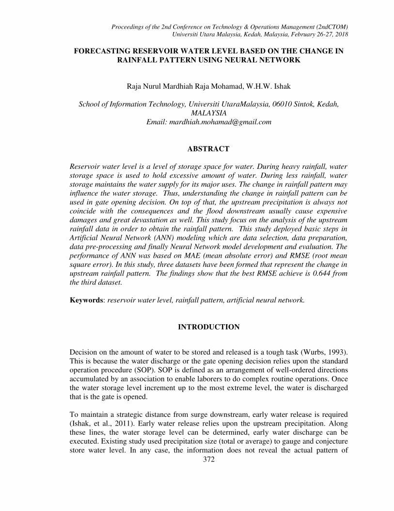
Figure 2

Neural Network Model for Data 1

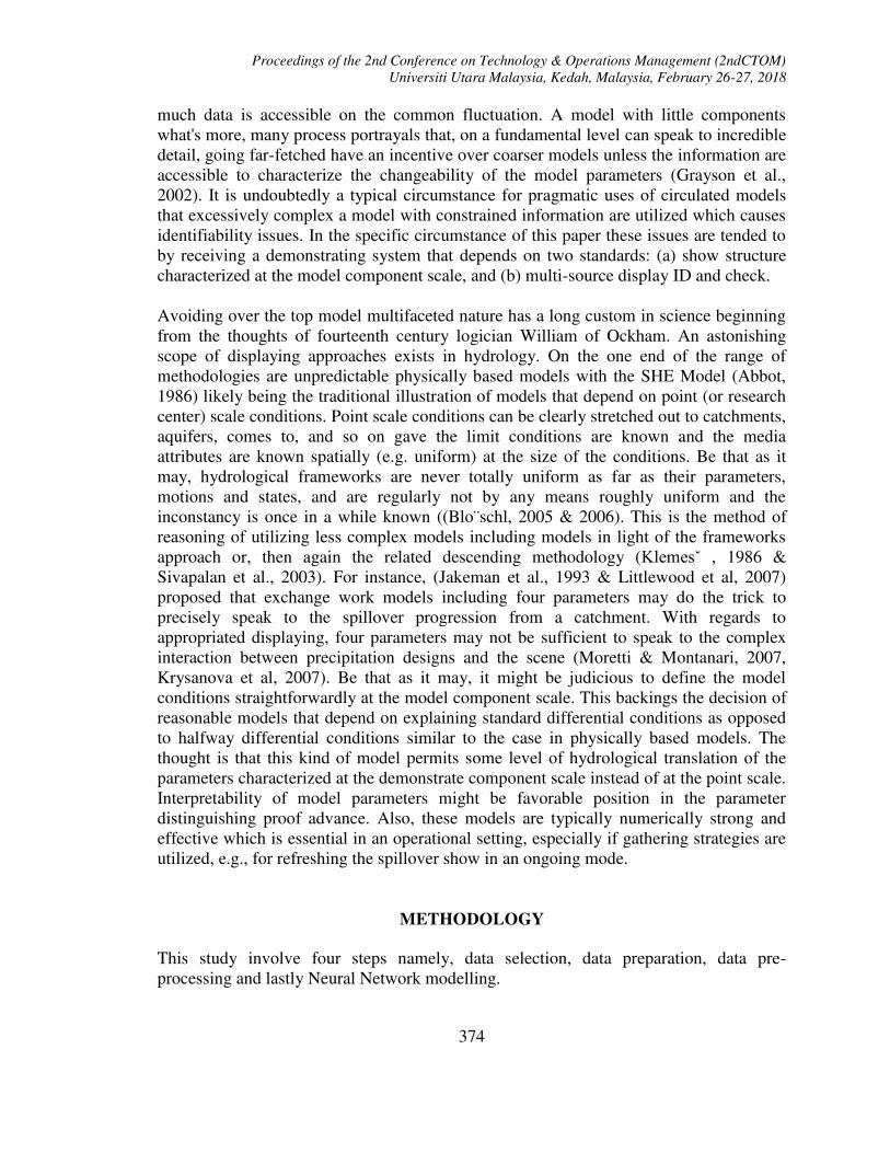
Figure 3




382

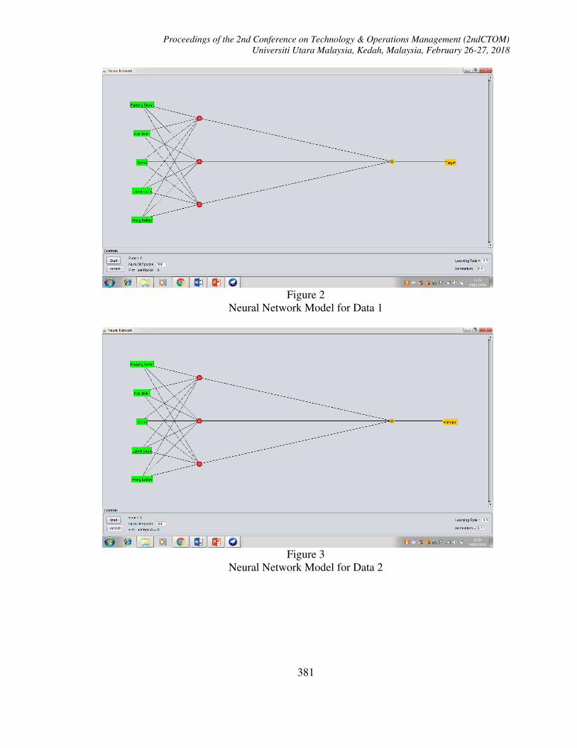
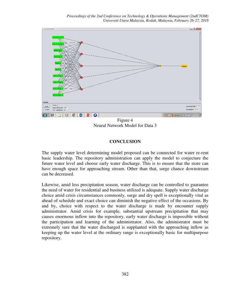
Figure 4


CONCLUSION

The supply water level determining model proposed can be connected for water re-rent

basic leadership. The repository administration can apply the model to conjecture the

future water level and choose early water discharge. This is to ensure that the store can

have enough space for approaching stream. Other than that, surge chance downstream

can be decreased.

Likewise, amid less precipitation season, water discharge can be controlled to guarantee

the need of water for residential and business utilized is adequate. Supply water discharge

choice amid crisis circumstances commonly, surge and dry spell is exceptionally vital as

ahead of schedule and exact choice can diminish the negative effect of the occasions. By

and by, choice with respect to the water discharge is made by encounter supply

administrator. Amid crisis for example, substantial upstream precipitation that may

causes enormous inflow into the repository, early water discharge is impossible without

the participation and learning of the administrator. Also, the administrator must be

extremely sure that the water discharged is supplanted with the approaching inflow as

keeping up the water level at the ordinary range is exceptionally basic for multipurpose

repository.



383

REFERENCES

Abbott, M.B., Bathurst, J.C., Cunge, J.A., O‘Connell, P.E., and Rasmussen, J. (1986). An

introduction to the European Hydrologic System e Syste`me Hydrologique

Europe´en, ‗‗SHE‘‘, 1, History and philosophy of a physically- based, distributed

modelling system. Journal of Hydrology 87, 45e49.

Anderson, Michael D., Walter C. Vodrazka Jr, and Rreginald R. Souleyrette (1998). Iowa

Travel Model Performance, Twenty Years Later. Transportation, Land Use and

Air Quality Conference.

Beven, K., (1989). Changing ideas in hydrology e the case of physically based models.

Journal of Hydrology, 105, 157-172.

Blo¨schl, G., (2005). On the fundamentals of hydrological sciences. In: Anderson, M.G.

(Ed.), Encyclopedia of Hydrological Sciences. J. Wiley & Sons, Chichester, pp. 3-

12.

Blo¨schl, G., (2006). Hydrologic synthesis e across processes, places and scales. Special

section on the vision of the CUAHSI National Center for Hydrologic Synthesis

(NCHS). Water Resources Research 42, W03S02, doi:10.1029/2005WR004319.

Blo¨schl, G., Zehe, E., (2005). On hydrological predictability. Hydrological Processes

19, 3923-3929.

Grayson, R., Blo¨schl, G., Western, A., and McMahon, T. (2002). Advances in the use of

observed spatial patterns of catchment hydrological response. Advances in Water

Resources 25, 1313-1334.

Ishak, W.H.W., Ku-Mahamud, K.R., Norwawi, N.M. (2011). Neural Network

Application in Reservoir Water Level Forecasting and Release Decision.

International Journal of New Computer Architectures and their Applications

(IJNCAA) ISSN 2220-9085 (Online), Vol. 1, No. 2, pp: 265-274

Jakeman, A.J., and Hornberger, G.M., (1993). How much complexity is needed in a

rainfall-runoff model? Water Resources Research 29, 2637-2649.

Klemesˇ, V., (1983). Conceptualisation and scale in hydrology. Journal of Hydrology 65,

1-23.

Krysanova, V., Hattermann, F., and Wechsung, F., (2007). Implications of complexity

and uncertainty for integrated modelling and impact assessment in river basins.

Environmental Modelling & Software 22 (5), 701-709.

Lehner, B., Doll, P., Alcamo, J., Henrichs, T., and Kaspar, F. (2000). Estimating The

Impact Of Global Change On Flood And Drought Risks In Europe: A

Continental, Integrated Analysis, Springer.

Littlewood, I.G., Clarke, R.T., Collischonn, W., and Croke, B.F.W., (2007). Predicting

daily streamflow using rainfall forecasts, a simple loss module and unit

hydrographs: two Brazilian catchments. Environmental Modelling & Software 22

(9), 1229-1239.

Loague, K.M., and Freeze, R.A., (1985). A comparison of rainfall-runoff modeling

techniques on small upland catchments. Water Resources Research 21, 229-248.

Loucks, D. P., J. R. Stedinger, and D. A. Haith (1981), Water Resources Systems

Planning and Analysis, Prentice-Hall, Englewood Cliffs, N. J.



384

Moretti, G., and Montanari, A., (2007). AFFDEF: a spatially distributed grid based

rainfall-runoff model for continuous time simulations of river discharge.

Environmental Modelling & Software 22 (6), 823-836.

Nash, Eamonn and Jonh Sutcliffe (1970). River Flow Forecasting through Conceptual

Models Part i—A Discussion of Principles. Journal of Hydrology 10(3), 282-290.

Parthasarathi, Pavithra and David Levinson (2010). Post-Construction Evaluation of

Traffic Forecast Accuracy. Transport Policy 17(6), 428-443.

Sarle, W. (1995). Stopped Training and Other Remedies for Overfitting. Proceedings of

the 27th Symposium on the Interface of Computing Science and Statistics, pp.

352-360. Retrieved March 18, 2002 from World Wide Web:

ftp://ftp.sas.com/pub/neural/.

Sivapalan, M., Blo¨schl, G., Zhang, L., and Vertessy, R., (2003). Downward approach to

hydrological prediction. Hydrological Processes 17, 2101-2111,

doi:10.1002/hyp.1425.

Stephenson, G.R., and Freeze, R.A., (1974). Mathematical simulation of subsurface flow

contributions to snowmelt runoff, Reynolds Creek Watershed, Idaho. Water

Resources Research 10, 284-294.

Wurbs, R. (1993). Reservoir-System Simulation and Optimization Models, Journal of

Water Resources Planning and Management, 119(4), 455–472,

doi:10.1061/(ASCE)0733-9496(1993)119:4(455)

Documents

FORECASTING RESERVOIR WATER LEVEL BASED ON THE …stmlportal.net/2ndCTOM/index.php/eProc181122/pdf/p372.pdf · Email: [email protected] ABSTRACT Reservoir water level is