Embed Size (px)
Citation preview

37t
140.
FORECASTING QUARTERLY SALES TAX REVENUES:
A COMPARATIVE STUDY
THESIS
Presented to the Graduate Council of the
North Texas State University in Partial
Fulfillment of the Requirements
For the Degree of
MASTER OF SCIENCE
By
Nancy A. Renner, B.S.
Denton, Texas
August, 1986
Renner, Nancy A., Forecasting Sales Tax Revenues:
A Comparative Study. Master of Science (Interdisciplinary
Studies--Applied Economics and Finance),, August, 1986
51 pp., 5 tables, bibliography, 24 titles.
The purpose of this study is to determine which of
three forecasting methods provides the most accurate
short-term forecasts, in terms of absolute and mean absolute
percentage error, for a unique set of data. The study
applies three forecasting techniques--the Box-Jenkins or
ARIMA method, cycle regression analysis, and multiple
regression analysis--to quarterly sales tax revenue data.
The final results show that, with varying success,
each model identifies the direction of change in the future,
but does not closely identify the period to period fluctu-
ations. Indeed, each model overestimated revenues for
every period forecasted. Cycle regression analysis, with
a mean absolute percentage error of 7.21, is the most accurate
model. Multiple regression analysis has the smallest
absolute percentage error of 3.13.

TABLE OF CONTENTS
PageLIST OF TABLES ......... . ........ iv
Chapter
I. OVERVIEW AND INTRODUCTION TO THE STUDY. . . .
OverviewIntroductionDescription of DataLimitations of the Study
II. REVIEW OF THE LITERATURE,....... .......... 5
IntroductionBackgroundRegression MethodsOther Studies and MethodsCycle Regression AnalysisCombining Forecasts
III. METHODOLOGY .............. ............ 22
IntroductionResearch TypeResearch ModelsApplication
IV. FINDINGS AND CONCLUSIONS.................33
IntroductionBox-Jenkins MethodCycle Regression AnalysisMultiple Regression AnalysisSummary TablesConclusions
APPENDIX............................ .. ........ 46
BIBLIOGRAPHY........................... . .......... 49
iii

LIST OF TABLES
Table Page
I. Box-Jenkins Method. ..... ....... 35
II. Cycle Regression Analysis . ........ 38
III. Multiple Regression Analysis......... ... e... 40
IV. Summary Tables. .... . ......... 42
V. MAPE--Two Time Horizons. . . ....... 43
iv
Nl'Ilw;----.--lW- mftllp

CHAPTER I
OVERVIEW AND INTRODUCTION TO THE STUDY
Overview
The purpose of this study is to determine which of three
forecasting methods provides the most accurate short-term
forecasts, in terms of absolute percentage error, for a
unique set of data. The study applies three time series
forecasting techniques--the Box-Jenkins method, cycle
regression analysis, and multiple regression analysis--to
quarterly sales tax revenue data. It introduces these
three methods and outlines the final models that were fitted
to the data.
Introduction
Time series analysis is an approach which has gained
increased use in forecasting since the late 1960s. "The
basic premise underlying time series methods is that the
best predictors of the future values of a data series are
the past values of the series itself" (2, p. 104). Time
series analysis can be divided into two categories--time
domain and frequency domain. In the former case, the
analysis is based on measuring and identifying the com-
ponents of a series. These components include trend, cycle,
1

2
seasonality, and random shocks. Examples of time domain
techniques range from very simple methods such as trend
lines and exponential smoothing to more sophisticated
techniques such as multiple regression and the Box-Jenkins,
or ARIMA, method. The acronymn stands for autoregressive
integrated moving average and represents the family of
models made popular by Box and Jenkins' book. These terms
are defined in Chapter III. (The reader will note these
two terms Box-Jenkins and ARIMA, are used interchangeably
in this study).
The second category, frequency domain techniques,
decomposes a time series into sine waves with varying fre-
quencies; therefore, the component parts are related to
frequency rather than time. Examples of this analysis
include the periodogram method, Fourier analysis, spectral
analysis, and cycle regression analysis (3).
These examples are only a sample of the numerous
forecasting techniques available to the analyst today.
With so many techniques available, the trend in fore-
casting is to look at these separate techniques not in
terms of winning and losing, but in terms of how each
differs from the other, and under what circumstances a
certain technique is most appropriate (1). In the same
manner, this study does not attempt to determine the

3
best of these three forecasting methods in the universal
sense but seeks only to identify the one that performs
most accurately on one time series data set.
Description of Data
The time series data employed in this study are a
set of 45 observations of quarterly sales tax revenues
for the City of Denton, Texas from the final quarter of
1974 to the final quarter of 1985. The data are listed in
Appendix A.
Limitations of the Study
This study evaluated only three forecasting techniques.
Clearly, there are numerous other methods that would have
been applicable to the quarterly time series data. The
data set was not large and was, therefore, a limitation;
furthermore, two methods only using 26 of the original 45
observations is a serious consideration.
The results of this study pertain only to the one
data set employed, and are not generalizable.
moswowi WOW Koolow " mWilmoomm-

CHAPTER BIBLIOGRAPHY
1. Makridakis, Spyros, Allan Andersen, Robert Carbone,Robert Fildes, Michele Hibon, Rodolf Lewandowski,Joseph Newton, Emmanuel Parzen, and RobertWinkler, "The Accuracy of Extrapolation (TimeSeries) Methods: Results of a ForecastingCompetition," Journal of Forecasting, 1 (1982),111-153.
2. McAuley, John J., Economic Forecasting for Business,Englewood, New Jersey: Prentice-Hall, Inc.1986.
3. Shah, Vivek, "Application of Spectral Analysis to theCycle Regression Algorithm," unpublished doctoraldissertation, North Texas State University, Denton,Texas, 1984:.
4

CHAPTER II
REVIEW OF THE LITERATURE
Introduction
In the first section of this chapter, two major fore-
casting studies are presented with emphasis on three
separate issues: (1) general findings, (2) common recom-
mendations, and (3) comments on the specific methods
employed in this thesis. In the second section, relevant
articles dealing with ARIMA models, multiple regression
analysis, and cycle regression analysis are reviewed.
The third section discusses the practice of combining
forecasting techniques.
Background
Two of the most comprehensive forecasting studies to
date are Mahmoud's "Accuracy in Forecasting: A Survey"
and "Accuracy in Forecasting: An Empirical Investigation"
by Makridakis, et al. The former study is a summary of
empirical investigations pertaining to forecasting. Special
emphasis is given to assessing the accuracy of different afore-
casting techniques (4). After reviewing approximately
120 sources, the author provides three general conclusions.
First, he found that
5

6
simple forecasting methods perform reasonably well
in comparison to the sophisticated forecasting
methods. Secondly, most of the studies indicate
that quantitative methods are more accurate than
qualitative methods. Thirdly, forecasting accuracy
can be improved by combining techniques (4, p. 155).
The Makridakis study analyzes and reports the results
of a forecasting competition in which expert participants
analyzed and forecasted many real life time series. (It
is usually referred to as the M-Competition.) The study
is concerned mainly with the post-sample forecasting
accuracy of the time series methods. Specifically, twenty-
four extrapolation methods were tested on 1001 time series
for 6-18 time horizons. (The Box-Jenkins, Lewandowski,
and Parzen methodologies used a sample of 111 time series)
(5).
The Makridakis study has been described as "the most
exhaustive undertaken to date in terms of number and variety
of extrapolation methods considered" (7, p. 273). Results
of the analysis show that (1) Lewandowski's method is
best for yearly and quarterly data, and both Holt and Holt-
Winter's exponential smoothing methods are equivalent;
(2) the Bayesian forecasting method and the Box-Jenkins
method are about the same as single exponential smoothing;
(3) on the macro level, the simple methods are superior
to the sophisticated methods; (4) on the micro level, the

7
sophisticated methods are the best; and (5) for seasonal
data, exponential smoothing, deseasonalized regression,
Bayesian forecasting and Parzen- methods are almost
identical (4).
One very clear finding, evident in both studies, is
that there does not exist one forecasting technique that
is "best" or "right" for every situation. In the commen-
tary on the M-Competition, one author listed that con-
clusion as one of the three major contributions of the
study (7). The authors of the M-Competition urge the fore-
casting user to discriminate in his/her choice of methods
according to the type of data (yearly, quarterly, monthly),
the type of series (macro, micro, etc.) and the time
horizon (5).
The two studies' recommendations are based on this
idea of no "best" technique. One should try "rather to
understand how various forecasting approaches and methods
differ from each other and how information can be provided
so that forecasting users can be able to make rational
choices for their situation" (5, p. 112). Mahmoud echoes
this conclusion by stating, "What is needed is an under-
standing of when and under what circumstances one method is
to be preferred over the other" (4, p. 154). The fore-
casting trend of the future, as recommended by Armstrong

8
and Lusk, is that "specific hypotheses should be formulated
and tested [as opposed to exploratory research] to
determine which methods will be most effective in given
situations" (2, p. 261).
Of the three methods being evaluated in this paper--
the Box-Jenkins method, cycle regression analysis, and
multiple regression analysis--the Box-Jenkins method
received the most attention in both the Mahmoud and
Makridakis studies. Simple linear regression trend fitting
is evaluated in both studies and will be presented as the
method most similar to multiple regression analysis. Cycle
regression analysis per se is not evaluated in either study.
As mentioned in Chapter I, the Box-Jenkins technique
is considered to be a sophisticated forecasting method and,
as such, its results are quite often compared to those of
the simple forecasting techniques in terms of accuracy.
Mahmoud concludes that simple forecasting methods perform
more accurately than, or at least as accurately as, sophis-
ticated methods. He cites three leading articles (one of
which is the M-Competition) that confirm this conclusion.
In his own study of fourteen time series, the Box-Jenkins
technique outperformed simple methods in only one series
(4).

9
Following are brief summaries of the findings of
studies reviewed by Mahmoud that employed the Box-Jenkins
technique:
1. The Box-Jenkins method and other quantitativemethods provided better forecasting than qual-itative ones in the majority of the studiescited.
2. Six studies reported that the Box-Jenkins methodwas superior to regression analysis. Onestudy indicated both methods performed aboutthe same.
3. The Box-Jenkins analysis was found to be 20percent more accurate than those using heuristics.
4. The Box-Jenkins method was found to be morerobust than econometric models in three studies;two studies showed that the Box-Jenkins methoddid at least as well as large econometric models.
5. Comparing Box-Jenkins and exponential smoothingmethods, one study showed Box-Jenkins superior,one study showed exponential smoothing superior,and one study showed them performing equally.
6. In a comprehensive study of 111 time series,(one by Makridakis that preceeded the M-Competition), results showed Box-Jenkins modelswere outperformed by the simple naive, movingaverage, and exponential smoothing methods (4).
The M-Competition evoked the following reactions and
observations regarding the Box-Jenkins method:
1. The participants stated that the Box-Jenkinsmethodology was the most time-comsuming (5).
2. Newbold questions how an "ARIMA model would beseriously outperformed by an exponential smooth-ing procedure which is really based on aspecific ARIMA model, which might have beenchosen. . . ignoring the presence of outlierscan lead to the choice of the 'wrong' ARIMAstructure" (9, p. 278).

10
3. Pack, a Box-Jenkins forecaster, defends time andhuman interference in the ARIMA methodology.He believes there were serious questions re-garding the validity of the experimental designof the M-Competition. These include a singleforecast time origin, averaging over differenttime series, averaging over lead times, andfocusing on a sequence of highly positivelycorrelated lead times (10).
4. The Box-Jenkins analyst of the M-Competition arguesthat, if the geometric mean squared one-step-ahead error is applied to the quarterly andmonthly series of the M-Competition, resultsshow, for short term forecasts, "The morecomplex techniques, in particular Box-Jenkins,are a little better; whereas for longer termforecasts it does not really matter whichmethod is used" (1, p. 287).
Makridakis, for whom the M-Competition is named, points
out that "sophisticated methods, such as Box-Jenkins . .
do their best on forecasts approximately three to four
periods ahead" (5, p. 297). He says, however, they were
designed to minimize the mean squared error on one-period
ahead forecasts. He theorizes that this discrepancy can be
attributed to the sophisticated methods "correctly identi-
fying the overall trend, but [not following] period-to-
period fluctuations because of the high amount of random-
ness involved" (5, p. 297).
Regression Methods
Since the relatively new cycle regression algorithm
was not incorporated in either Mahmoud's survey or the

11
M-Competition, findings concerning the regression method
must be addressed. In Mahmoud's survey, regression analysis
was compared to moving average and exponential smoothing in
four different studies from 1965-1972. Results showed
that regression analysis was the most accurate technique
for longer-term forecasts; however, it was consistently
outperformed by the other two techniques in short-term
forecasts. In 1981, a study by Dalrymple and King comparing
these three techniques indicated that the regression
method was the most accurate used in the study (4). Linear
regression analysis, however, did not fare as well in the
M-Competition. In fact, it was considered one of the worst
overall forecasting tools (5). However, deseasonalized
regression analysis used on seasonal data had approximately
the same overall mean absolute percentage error as expo-
nential smoothing, the Bayesian method, and the Parzen
method (4). A summary statistic of the M-Competition
estimated the percentage of time that the Box-Jenkins
method is better than the regression method. For the
first four forecasting horizon periods, those percentages
are 64.0, 68.5, 72.1, and 65.8 respectively (5). (It
should be noted that this is simple linear regression
analysis, not multiple regression analysis.)

12
Other Studies and Methods
This section briefly covers additional literature on
the Box-Jenkins method and regression models. It also
introduces the development of cycle regression analysis.
The Box-Jenkins technique has become quite popular
since the publication of their book, Time Series Analysis,
Forecasting and Control, in 1970. Throughout the 1970s,
this technique was compared to other forecasting methods.
Some researchers believe the popularity of the Box-Jenkins
method was based on the fact that several studies found it
to be at least as accurate as the complex econometric models
of the U. S. economy (5). One such study, for example,
concluded "the Box-Jenkins results were significantly
better in all cases and, except for GNP, they provide better
forecasts by a factor of almost two to one" (8, p. 153).
Numerous other studies reached similar conclusions; however,
some researchers concluded that it was the inability of
econometric models to accommodate structural change in the
economy that truly gave the ARIMA models the edge (6). In
at least one study, the outcome was reversed between
these two methods, and the ARIMA model was the worst
performing of the two compared (6). Other studies comparing
Box-Jenkins with methods such as exponential smoothing,
moving averages, stepwise autoregression, etc. are equally

13
as contradictory; yet, until Makridakis & Hibron (1979),
Makridakis et al (1982), and Mahmoud (1982), the Box-
Jenkins method was generally believed to be at or near the
top of the forecasting techniques. As seen earlier in
this chapter, these more recent studies have reversed this
thought; however, these particular studies are not completely
accepted. There continues to be questions regarding the
ability of the particular analyst in a specific study to
fit precisely the proper Box-Jenkins model, so a fair
comparison can be made.
The majority of the literature in the last decade
dealing with regression forecasting techniques has centered
around econometric models. These structural models are
usually quite complex and use numerous equations containing
mainly macroeconomic variables (3). Multiple regression
analysis then is a simplified version of these larger
models.
In 1972, Cooper compared regression forecasts and auto-
regressive forecasts of thirty-three dependent variables
from seven macroeconomic models. Results showed the auto-
regressive models outperformed the regression models in
eighteen of thirty-three cases (3). Similar conclusions
were reached by Cooper and Nelson when they compared the
Federal Reserve Bank of St. Louis' regression method and an

14
autoregressive model on forecasts of six variables. One
year later, Behravesh found forecasts obtained from
regressive equations to be superior to those generated
by an autoregressive scheme (3). Another study, titled
"The Forecasting Record of the 1970's," compared econo-
metric models only to other econometric models. As the
M-Competition and Mahmoud's survey showed, no one fore-
casting technique was the most accurate for the seventeen
variables reviewed. Each technique had strengths and
weaknesses (3) .
As noted with the somewhat contradictory studies of
Box-Jenkins methodology, not all regression models perform
equally well. In fact, just as the Box-Jenkins analyst
of the 1980s attributes the poor performance of the ARIMA
method to the misspecification of the model, the econo-
metricians of the 1970s felt that their methods were also
being applied inappropriately and therefore were not actually
outperformed by the ARIMA models (5; 10).
Finally, a study incorporating both an ARIMA model
and regression analysis must be considered. These two
methods were applied to monthly sales tax revenues, and fore-
casts were made for five months. Multiple regres ion analysis
was utilized with a trend variable and dummy variables
for seasonality. With few exceptions, this is the regression

15
model used in this thesis. Final results showed that the
ARIMA model and the regression method had average absolute
percentage errors of 3.2 percent and 3.6 percent, respec-
tively. The author concluded that "both techniques capture
the directional changes. . . but neither method anticipated
the sharp drop in receipts" in the final forecasting period
(3, p. 387). The study pointed out that the higher cost
of constructing and maintaining the ARIMA model could
make the regression model the more attractive of the two
methods, even though the ARIMA model slightly outperformed
it (3).
Cycle Regression Analysis
The final method used in this study is the frequency
domain technique called cycle regression analysis. It was
first introduced by Simmons and Williams in 1982. The
family of frequency domain techniques includes Fourier
analysis, spectral analysis, the periodogram, and the
Cosinor test. Until recently, these techniques have been
used extensively and successfully in biological and
physical sciences as well as in engineering. Now they
are being adapted to the business world (15).
The other methods have limitations which cycle
regression attempts to overcome. For example, unlike the
periodogram, cycle regression analysis is not restricted

16
to equally spaced observations. The Cosinor test and the
periodogram method require a priori knowledge of the
sinusoidal periods. The cycle regression method does not
require such knowledge; therefore, it is more objective
than the other two methods. The Fourier method also
requires a priori knowledge of "either the number of
trigonometric terms to be included or the fundamental
frequency" (12, p. 46). Again in cycle regression analysis,
these are done objectively by the heuristic steps of the
method (13).
In their 1982 introductory article, Simmons and Williams
found cycle regression analysis superior to the period-
ogram method in estimating amplitudes, angular frequencies,
and phases. The algorithm was also successful in fore-
casting Texas Instrument common stock prices in the short-
term future (15). A second study, by the same authors,
compared cycle regression analysis with stepwise multiple
regression analysis for three separate dependent variables:
political regime, civil conflict, and energy consumption.
In every case, cycle regression analysis had a higher
percentage variation explained than did multiple regression
analysis (16) .
Although the cycle regression algorithm used in
this study is objective and automatic (computer generated
with no human interference), this is not true of the algorithm
17
used in the two studies previously discussed. The one
subjective step in the earlier algorithm involved analyzing
the autocorrelations of the residuals to find an initial
estimate for the cycle period. Specifically, the analyst
was required to determine significant valleys and subsequent
peaks in the autocorrelations. Designation of significance
was left to the analyst's judgment (14). Since 1983,
three methods have been presented to eliminate this sub-
jective step. Two of the methods will be discussed here;
the second method is the one employed in this study.
Simmons et al first developed an objective method
that employed a t-like statistic to determine when "the
autocorrelations have dropped to a significant negative
value, and increased to a significant positive value"
(14, p. 99-100). The method was based upon a procedure
involving sample autocorrelations from the Box-Jenkins
methodology. Validation tests of this procedure show that,
in almost all cases, "estimates obtained by the t-value
method were closer to the true periods than those obtained
by the original procedure" (14, p. 100). Their second
method incorporates spectral analysis in estimating the
cycle period. Validation tests on the technique currently
are being conducted; preliminary findings show that the
spectral analysis step enhances the overall analytical
capabilities of cycle regression methodology (13).

13
Combining Forecasts
In Mahmoud's survey of forecasting techniques, an
entire section is dedicated to reviewing the literature
on combining techniques. Without exception, every study
he reviewed reported some type of improvement when a
composite forecast was used (4). Although there are a
number of methods of combining techniques, this study will
limit itself to taking a simple average of forecasts. The
M-Competition chose only to look at two methods of combining
forecasts--the simple and the weighted average methods.
The author called the simple average "Combining A," and
it consisted of an average of the following six methods:
exponential smoothing, adaptive response rate exponential
smoothing, Holt's exponential smoothing, Brown's linear
exponential smoothing (all of which were deasonalized),
Holt-Winters linear and seasonal exponential smoothing, and
the Automatic Carbone-Longini. "Combining A" was a weighted
average based on the sample covariance matrix of percentage
errors of the same six methods (5). Both "Combining A"
and "Combining B" performed better than virtually all of
the individual methods, including the six methods used in
the combination, as well as the other methods in the
M-Competition; futhermore, the simple average technique
performed better than the weighted average method (5).

19
A later study by Makridakis and Winkler, however,
showed differential weighting outperforming a simple
average method (4). The most recent study by Makridakis
and Winkler evaluated only simple average combinations.
Fourteen forecasting methods and 111 time series were used.
The following three conclusions were reached: (1) The
specific methods included in a combination had little
influence on the accuracy of the forecasts; (2) although
accuracy increased with each additional method used, a
saturation point was reached after four or five methods;
(3) as the number of methods used in a particular combination
increased, the variability of the accuracy of the different
combinations decreased (4).
In conclusion, Reeves and Lawrence point out that
interactive computer forecasting packages allow analysts
to produce multiple forecasts with respect to a single
objective. Generally, "The single forecast which comes
closest to satisfying the chosen objective is then selected,
and the remaining forecasts are discarded" (11, p. 271).
They believe this process may not make the best use of
all the available information because discarded infor-
mation may contain information not available in the
selected forecast. This is possible because the discarded
information may be based on "different assumptions, dif-
ferent variables, or different relationships among variables"
(11, p. 271).
ONOW"Al ANN

CHAPTER BIBLIOGRAPHY
1. Andersen, Allan, "Viewpoint of the Box-Jenkins Analystin the M-Competition," Journal of Forecasting,2 (1983), 286-287.
2. Armstrong, J. Scott and Edward J. Lusk, "The Accuracyof Alternative Extrapolation Models: Analysis ofa Forecasting Competition through Open PeerReview," Journal of Forecasting, 2 (1983), 259-262.
3. Bails, Dale G. and Larry C. Peppers, Business Fluctu-ations--Forecasting Techniques and Applications,Englewood iff7 New Jersey: Prentice-Hall,Inc., 1982.
4. Mahmoud, Essam, "Accuracy in Forecasting: A Survey,"Journal of Forecasting, 3 (1984) , 139-159.
5. Makridakis, Spyros, Allan Andersen, Robert Carbone,Robert Fildes, Michele Hibon, Rudolf Lewandowski,Joseph Newton, Emmanuel Parzen, and Robert Winkler,"The Accuracy of Extrapolation (Time Series)Methods: Results of a Forecasting Competition,"Journal of Forecasting, 1 (1982), 111-153.
6. Makridakis, Spyros and Michele Hibon, "Accuracy ofForecasting: An Empirical Investigation,"Journal of the Royal Statistical Society, A(1979), 142, Part 2, 97-145.
7. Markland, Robert E., "Does the M-Competition Answerthe Right Questions?," Journal of Forecasting,2 (1983), 272-273.
8. Naylor, Thomas H. and T. G. Seaks, "Box-Jenkins Methods:An Alternative to Econometric Models," Inter-national Statistical Review, 40 (1972), (2), 113-137.
9. Newbold, Pau.l "The Competition to End all Competitions,"Journal of Forecasting, 2 (1983), 276-279.
20
21
10. Pack, David J., "What Do These Numbers Tell Us?,"Journal of Forecasting, 2 (1983), 279-285.
11. Reeves, Gary R. and Kenneth D. Lawrence, "CombiningMultiple Forecasts Given Multiple Objectives,"Journal of Forecasting, 1 (1982), 271-279.
12. Shah, Vivek, "Application of Spectral Analysis to theCycle Regression Algorithm," unpublished doctoraldissertation, North Texas State University, Denton,Texas, 1984.
13. Simmons, LeRoy F., "The Complete Family of CycleRegression Algorithms," Proceedings of the South-west Region American Institute for DecisionSciences, 1986.
14. Simmons, LeRoy F., Mayur R. Mehta and Laurette PoulosSimmons, "Cycle Regression Analysis Made Objective--The T-Value Method," Cycles, 24 (1983), 99-102.
15. Simmons, LeRoy F. and Donald R. Williams, "A CycleRegression Analysis Algorithm for ExtractingCycles from Time Series Data," Journal ofComputers and Operations Research, An InternationalJournal, 9 (1982), 243-254.
16. Simmons, LeRoy F. and Donald R. Williams, "The Use ofCycle Regression Analysis to Predict CivilViolence," Journal of Interdisciplinary CycleResearch, An International Journal, 14 (1983),203-215.

CHAPTER III
METHODOLOGY
Introduction
This chapter outlines the time series methodology
employed in this study. Specifically, it discusses (1)
the research type, (2) the research models and (3) the
application of the models.
Research Type
In this paper, time series analysis is tested for its
forecasting capabilities. Time series analysis can be
divided into two categories, time domain and frequency
domain, as defined in Chapter I. Of the three types of
time series analysis tested, two--Box-Jenkins and multiple
regression--are time domain; the third--cycle regression--
is a frequency domain technique. The two time domain
techniques can also be subcategorized as follows: Box-
Jenkins is an extrapolation method which predicts future
values based on relevant statistical features of past
data (1). Multiple regression is considered a causal
model.
22

23
Research Models
Three distinct models were used in this study. In
statistical forecasting, a model is defined as an "algebraic
statement telling how one thing is statistically related
to one or more other things" (5, p. 5). The first model
tested in this study is the Box-Jenkins or ARIMA model.
Basically, Box-Jenkins is an algebraic statement showing
how "observations on the same variable are statistically
related to past observations on the same variable"
(6, p. 5). It is important to note that an ARIMA model
is really a family of models from which the researcher
chooses the most appropriate specification.
Box-Jenkins analysis is based on the idea that the
time-sequenced observations in a data series may be statis-
tically dependent. An ARIMA model can include both an
autoregressive term (AR) and a moving average (MA) term.
An AR term is expressed as a function of past values of
itself at varying time lags. The MA term is a function of
previous error values. In addition, differencing enters
the period to period change in the series. (It can be
expressed algebraically as: Xt t Xt-.) The I in
ARIMA stands for integrated, which is the process that
converts the differenced series back to the original forms
(5). Algebraically, the AR and MA terms are expressed:

24
AR (1): zt = C + 0z t-l + at
MA (1): zt = C -0 at-l + at
where zt is the variable whose time structure is described
by the process; C is a constant term related to the mean
of the process; 01zti is the AR term and is a fixed
coefficient, 01, multiplied by a past z term; 0 1at-1 is the
MA term and 01 is a fixed coefficient multiplied by a past
random shock, at'-l; and at is a current random shock (6).
The ARIMA model is further described as an ARIMA
(pdq)(P4,D,Q)s where p is the nurber of lagged autoregressive
terms, d is the order of differencing used to make the
series stationary, and q is the number of lagged errors,
or shocks, in the moving average component. The capital
letters (P, D, Q) represent the seasonal component in
the model. The s is the periodicity of the process. The
actual development of the model involves three stages
(5):
1. Identification. One of the keys to this stageis transforming the time series so it is sta-tionary. Transformation options include log-arithms, raising to powers, and centering. Anadditional transformation for eliminating trendor drift is differencing. Plots of the estimatedautocorrelation functions (acf) and partialautocorrelation functions (pacf) are examinedto give the researcher a feel for any patternsin the data. An autocorrelation function is agraphic representation of autocorrelation coef-ficients. These coefficients "measure the
-will, OWN 0 'A"Wimmi

25
direction and strength of the statisticalrelationship between ordered pairs of obser-
vations on two variables" (6, p. 35). The
partial autocorrelation function is similarto the acf, but instead of representing the
relationships only between ordered pairs,the pacf takes into account the effects
of intervening values (6). The acf and
pacf are then used as guides for choosingan appropriate ARIMA (p,d,q) (P,Q,D)s model.
2. Estimation. Estimates of the coefficients
0 and 8 are chosen during this stage. An
iterative nonlinear estimation process is used.Several computer programs perform this esti-mation.
3. Diagnostic Checking. This stage primarily
checks that the random shocks (a ) are inde-
pendent. Since one cannot actually observeshocks, the residuals (at) are observed.More precisely, a residual acf is constructed,and t-values and the summary Box-Pierce chi-
square statistic are calculated (6). TheBox-Pierce statistic is used to "determine
whether several autocorrelation coefficients
are significantly different than zero" (4,p. 269). It is based on the chi-squareddistribution of the autocorrelation coef-
ficients. If the autocorrelation coefficients
are not significantly different from zero,the data generating those autocorrelationsare considered random (4). If these diagnostic
checks do not prove satisfactory, the iterativeprocess, common in ARIMA modeling, is begunagain.
The second method used in this study is a cycle
regression algorithm involving spectral analysis. The
algorithm estimates the sinusoidal or harmonic components
in times series data. This is done by employing Marquardt's
compromise to estimate amplitude, period, and phase
simultaneously (8). Marquardt's compromise is a nonliner

26
regression procedure that accurately and quickly con-
verges to least squares estimates (6).
Spectral analysis is used in this algorithm to
determine the initial period of the harmonic. Technically,
the method is used to estimate the angular frequency of
the dominant harmonic which is in turn used to estimate
the period. The spectral analysis method estimates a
spectrum, or the spectral density function, of the time
series being analyzed. Its primary objective is to deter-
mine the "most significant components in terms of their
contribution to the total variance in the data" (7, p. 23).
A spectrum decomposes this total variance into that explained
by components of various frequencies. In this way,
spectrums can be used to detect sinusoidal components in
the data (7).
The following steps outline the general algorithm
for cycle regression. They include a "starting procedure
that fits trend and one harmonic, steps for adding addi-
tional harmonics, and a stopping procedure" (8, p. 31).
Step 1: The starting procedure is to estimate thetrend and first harmonic. Linear regressionis used to obtain the initial estimates ofthe intercept and slope parameters. Auto-correlations are computed from residuals,and the spectral density function is computedfrom these autocorrelations (8). Thespectral density function is estimated at

27
different frequencies with the frequencycorresponding to the highest peak, (i.e.,highest spectral density function value)singled out. This frequency is multipliedby 21r to obtain the initial estimate ofthe angular frequency of the dominantharmonic (7; 8).
The initial estimate is used by cycle regression analysis
to determine the estimates of amplitude, phase, and
period of the harmonic (7). It is at this point that
Marquardt's Compromise is used to move from the initial
estimates described above to the final estimate for
the trend and the first harmonic. The appropriate equation
is as follows:
Xt = B0 + B t B2 Sin B3 (t + B4 ) + et
where:
B + B1 t represents the linear trend;
the parameters B2 , B3 and B4 determine the amplitude;
period, and phase respectively of the first harmonic;
et is a random variable (7).
The stopping procedure involves a partial F-test to
establish significance of the harmonic. If it is not
found significant, Step 1 is repeated. If it is found to
be significant, Step 2 is followed.
Step 2: Parameters for k harmonics when k = 1 areestimated in this step. Estimates obtainedfor trend in Step 1 are used again. Forthe initial estimate of B (angular fre-quency), the estimate froAB3 is used for

28
all harmonics until the kth harmonic wherethe spectral density function procedure isused to obtain the initial estimate. Forthe initial estimate of B3+ (phase), theestimate of B in Step 1 is used for allharmonics except the kth harmonic. Themodel uses 0.1 for that harmonic. For theinitial estimate of B31 (amplitude),the amplitudes found ir tep 1 are summedand divided by k. The final estimates fortrend and k harmonics are found throughMarquardt's compromise using the aboveestimates in the following equation:
K
Xt 0 1B + B t + :F.. B3i-l Sin B3i (t + B3i+l) + eti=1
The stopping procedure again applies a partial F-test to
determine the significance of the kth harmonic. If signi-
ficance is established, k is increased by 1, and Step 2
is repeated. If it is not significant, the model obtained
from the equation above is used. (8; 7).
The third method employed in this study is multiple
regression analysis. It is merely an extension of simple
linear regression, and attempts to explain changes in the
dependent variable (Y) in terms of changes in two or more
independent variables (X1 X2 ' . . X). In this study,
as in many regression studies, dummy variables are used
to account for seasonal variation in the data. In general
terms, the multiple regression model is written:
Y = a + b X + bX + . b + X + e= 1 t 2t k kt t
29
where Y represents the dependent variable whose values are
explained by the model. Parameters a and b are estimated
by the least squares principle; a is considered the inter-
cept and b is described as a partial slope since the
regression equation no longer fits a simple straight line,
and e denotes the error term (3). The error term is a
very important factor when applying multiple regression
analysis to time series data. As in the ARIMA model,
the researcher must be aware of the possibility of auto-
correlated error terms. Examining the autocorrelations
of the residuals visually as well as calculating the
Durbin-Watson statistic are two means of testing for auto-
correlation. The Durbin-Watson statistic tests for the
most important type of autocorrelation--first-order
linear correlation. The statistic is defined as the "ratio
of the sum of squares of successive differences of resi-
duals to the sum of the squared residuals" (2, p. 161). A
value of approximately 2 indicates the absence of first
order autocorrelation (2).
Application
The time series data analyzed in this study are
quarterly sales tax revenues for the City of Denton, Texas
from the final quarter of 1974 to the final quarter of
1985. This constitutes 45 observations; however, the ARIMA

30
model eventually fit the last 26 observations only. The
pattern of the data appeared to change around the 20th
observation; consequently, after numerous attempts at
fitting an ARIMA model to the entire set proved unsuccess-
ful, the decision was made to model the most recent 26
observations. The same decision was made with regard to
the cycle regression model. The multiple regression model,
however, used the original data in its entirety.
The final ARIMA model, using (p, d, q) (PI, D, Q)s
notation, is (0,1,0) (1,1,1)4. To achieve a more stationary
time series, a natural logarithmic transformation was
performed. The nonseasonal component fits one auto-
regressive term and one moving average term, both at lag
four. Seasonal differencing completes the final model.
The ARIMA model was chosen using two statistical
packages--IDA and Minitab. Minitab was only used in cal-
culating initial estimates for the parameters needed in
the model. IDA was used primarily in a trial and error
fashion with the acf and pacf plots, histograms, and the
Box-Pierce statistic serving as the major sources of
feedback.
The cycle regression method was applied through a
computer program obtained from Dr. LeRoy Simmons of the
Business Computer Information Systems Department of North

31
Texas State University. All parameters needed for the
final forecasting model were computed automatically by
Dr. Simmons' program. A short program that can be run on
an IBM personal computer was written to solve the final
forecasting equation. The final cycle regression model
fit three significant harmonics to the tax revenue data.
In the multiple regression model, the quarterly tax
revenues served as the dependent variable, and six inde-
pendent variables were assigned to the equation. X was
a dummy variable that basically divided the data set into
two sections--before and after the 20th observation;X12
was time (1 . . . 45) which accounted for trend; X was
time squared which accounted for the nonlinearity of the
time series; X4 through X6 were dummy variables representing
the seasonal factor of the quarterly data. The statistical
package of SPSSx was used for this regression analysis.
Chapter IV presents the final equations used in these
three models. The point forecasts, generated from these
equations, are discussed, and interpretations and con-
clusions are given.

CHAPTER BIBLIOGRAPHY
1. Gilchrist, Warren, Statistical Forecasting, New York:John Wiley and Sons, 1976.
2. Intriligator, Michael D., Econometric Models, Techniques,and Applications, Englewood Cliffs, New Jersey:Prentice-Hall, Inc., 1978.
3. Lewis-Beck, Michael S., Applied Regression An Introduction,Beverly Hills: Sage Publications, 1980.
4. Makridakis, Spyros, S. C. Wheelwright and V. E. McGee,Forecasting Methods and Applications, 2nd edition,New York: John Wiley and Sons, 1983.
5. McAuley, John J., Economic Forecasting for Business,Englewood Cliffs, New Jersey: Prentice-Hall, Inc.,1986.
6. Pankratz, Alan, Forecasting With Univariate Box-JenkinsModels, New York: John Wiley and Sons, 1983.
7. Shah, Vivek, "Application of Spectral Analysis to theCycle Regression Algorithm," unpublished doctoraldissertation, North Texas State University, Denton,Texas, 1984.
8. Simmons, LeRoy F., "The Complete Family of Cycle RegressionAlgorithms," Proceedings of the Southwest RegionAmerican Institute for Decision Sciences, 1986.
32
CHAPTER IV
FINDINGS AND CONCLUSIONS
Introduction
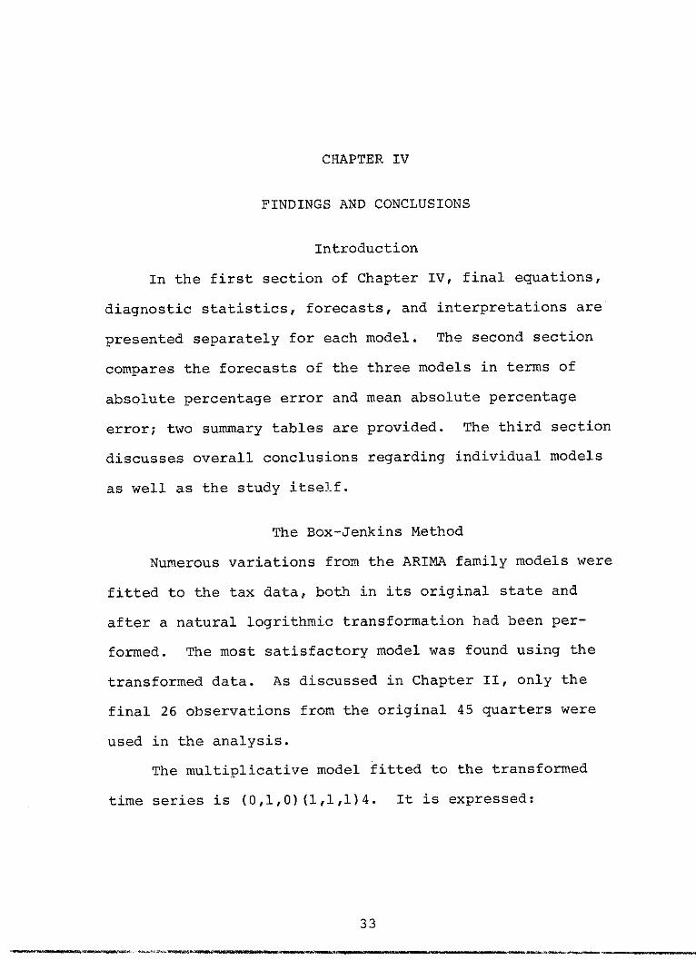
In the first section of Chapter IV, final equations,
diagnostic statistics, forecasts, and interpretations are
presented separately for each model. The second section
compares the forecasts of the three models in terms of
absolute percentage error and mean absolute percentage
error; two summary tables are provided. The third section
discusses overall conclusions regarding individual models
as well as the study itself.
The Box-Jenkins Method
Numerous variations from the ARIMA family models were
fitted to the tax data, both in its original state and
after a natural logrithmic transformation had been per-
formed. The most satisfactory model was found using the
transformed data. As discussed in Chapter II, only the
final 26 observations from the original 45 quarters were
used in the analysis.
The multiplicative model fitted to the transformed
time series is (0,1,0)(1,1,1)4. It is expressed:
33

34
0(B )VdV D = e (B )4 zt Q at
where
0(B4) is the seasonal autoregression term at lag 4,
V d VDis nonseasonal differencing at length 1multiplied by seasonal differencing at length 4
zt is the variable whose time structure is describedby the process
eQ(B ) is the seasonal moving average term at lag 4
at represents random shocks
(Note: B represents backshift notation where B4zt = z t -
(8). The following parameter estimates are used in the
equation:
seasonal autoregressive coefficient (0) = -.9seasonal moving average coefficient (e) = .65
Both coefficients are significant at the .05 level with
t-values of 86.46 and 6.05, respectively. The Box-Pierce
statistic is 17.96, which is below the critical value of
30.1 for 19 degrees of freedom (8). This statistic, as
discussed in Chapter III, is a test for correlation among
the random shocks of a time series and is based on the
residual autocorrelations.
Forecasts of sales tax revenues for two time horizons
(the first two quarters of 1986) were calculated from this
model. Table I shows the forecasts, the actual revenues,
and the absolute percentage errors.

35
Table I
BOX-JENKINS METHOD
Absolute
Time Horizon Actual Forecast Percentage Error
1 $1,270,681 $1,420,057 11.76
2 $1,119,925 $1,295,177 15.65
The Box-Jenkins model projects revenues of $1,420,057
for the first quarter of 1985. This is approximately
$150,000 over the actual revenues generated for that
quarter. The second quarter projection is approximately
$175,250 over the actual amount generated. The absolute
percentage errors (APE) of 11.76 and 15.63 were the largest
of the three models used in the study. These two errors
produce a mean absolute percentage error (MAPE) for the
combined time horizons of 13.71. The M-Competition reported
the MAPE for the Box-Jenkins methodapplied to quarterly
data for the time horizons 1 and 2,as 7.6 and 8.2, respec-
tively (4).
There are several possible explanations for these
large errors. The most obvious is rather simple and
straightforward--the model was not specified correctly.
The Box-Jenkins methodology is complex, and most analysts

36
believe time and experience are required to truly fit the
proper models consistently. In fact, C.W.G. Granger noted
that "it has been said to be so difficult that it should
never be tried for the first time" (6, p. 112). In
addition, the amount of subjectivity in fitting the model
allows for a wide range of possible solutions; consequently,
the risk of not specifying the "right" process increases.
In the M-Competition commentary, Geurts states "that it
is probable for two experienced Box-Jenkins forecasters to
examine identical autocorrelations, partial autocorre-
lations. . . and then to specify different models" (2, p. 268).
Another possibility is that the overall trend is being
detected, since the direction of both forecasts are correct,
but the process is not following the "period-to-period
fluctuations because of the high amount of randomness"
(5, p. 297).
Cycle Regression Analysis
The most satisfactory cycle regression model, in terms
of forecasting, used only the final 26 observations of the
time series. This abbreviated set of data limited the
search for significant harmonics. Instead of proceeding
until an insignificant one was identified, the algorithm
stopped after three significant harmonics were identified.
This is due to a limit imposed by the program. In an

37
attempt to prevent overfitting of the data, half the
number of observations is the maximum number of parameters
that can be used in this program; therefore, with 26
observations, the program will fit a maximum of 13 parameters.
Since each sine wave has three parameters, (amplitude,
period, and phase) and trend accounts for two more para-
meters (constant and slope), a fourth harmonic would have
fit a total of 14 parameters--one more than the maximum
allowed by the program.
As outlined in Chapter II, the general equation for
cycle regression analysis is
xt = B0 + Blt + B2Sin B3(t + B 4 + et
where
B and B are the intercept and slope parameters,0 .litrespectively
B2 , BA, B4 are the parameters for amplitude, period,and p ase respectively
et is a random variable (9).
The following equation includes the final parameters
generated by the cycle regression algorithm:
Y = 380069.4 + 30325.12t+ 67998.81sin(.2923369(t+2.024837))+ 79239.75sin(3.128417(t+.1025962))- 58777.58sin(l.546734(t+.6198372))
t = 27, 28
Table II presents the forecasts, the actual revenues,
and the percentage errors for the cycle regression method.

38
TABLE II
CYCLE REGRESSION ANALYSIS
AbsoluteTime Horizon Actual Forecast Percentage Error
1 $1,270,681 $1,359,366 6.982 $1,119,925 $1,203,288 7.44
The forecast generated from cycle regression analysis
overestimates revenues for two time horizons by $88,685
and $83,363, respectively. This method provided the
smallest MAPE (7.21) of the three methods used in the study.
Since this method requires no human intervention, subjectivity
is not an issue. There are, however, certain advantages and
disadvantages that can be addressed. The method's objective-
ness allows for extremely quick and easy forecasts. The
only time consuming step is solving the final equation,
and this step was shortened considerably by a basic program
run on a personal computer. One disadvantage of the method
is its relatively newness to the family of frequency domain
techniques. It has not been tested to the extent of the
other two methods. In addition, the program for cycle
regression analysis cannot, at present, be purchased in a
large statistical package as can the other two methods.
M&A

39
Multiple Regression
All 45 observations of the time series data are included
in the multiple regression model. Tax revenue serves as
the dependent variable, and it is regressed on six indepen-
dent variables. Of the six independent variables used,
four are dummy coded. (Descriptions of the variables are
provided at the end of Chapter III.) The following equation
represents a multiple regression model with six independent
variables.
Yt = a + b1 X1 t + b2 tX2 . . . + B6X 6t + et
To forecast from this equation for two time horizons,
t is given the values of 46 and 47, and the coefficients
for a, b, and XI through X6 are inserted:
Y = 242581.38 + 9387.24 + 1772.17(46) + 432.96(46 2+ 60770.90
Y = 242581.38 + 9387.24 + 1772.17(47) + 432.96(47 2- 36787.63
(Note: In quarter 46, X4 and X6 have values of zero; in
quarter 47, X4 and X5 have values of zero)
The value of 2.03 for the Durbin-Watson statistic is
significant at the .05 level. To accept the null hypothesis,
i.e., to conclude that first order autocorrelation is not
present, the following equation must be satisfied:
du(d (4 - du
where du, for n = 45 and k = 7, = 1.24
1.24(2.03(2.76 (7;3).
MAW,
40
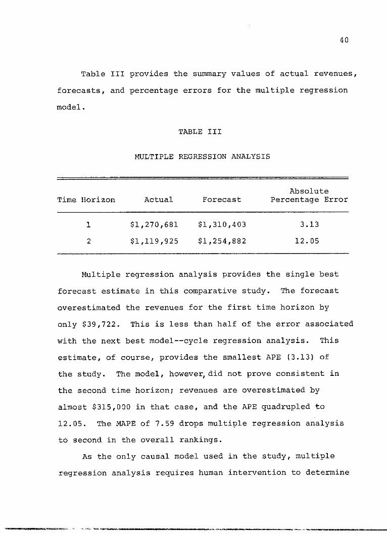
Table III provides the summary values of actual revenues,
forecasts, and percentage errors for the multiple regression
model.
TABLE III
MULTIPLE REGRESSION ANALYSIS
AbsoluteTime Horizon Actual Forecast Percentage Error
1 $1,270,681 $1,310,403 3.13
2 $1,119,925 $1,254,882 12.05
Multiple regression analysis provides the single best
forecast estimate in this comparative study. The forecast
overestimated the revenues for the first time horizon by
only $39,722. This is less than half of the error associated
with the next best model--cycle regression analysis. This
estimate, of course, provides the smallest APE (3.13) of
the study. The model, however, did not prove consistent in
the second time horizon; revenues are overestimated by
almost $315,000 in that case, and the APE quadrupled to
12.05. The MAPE of 7.59 drops multiple regression analysis
to second in the overall rankings.
As the only causal model used in the study, multiple
regression analysis requires human intervention to determine
m'oft

41
the number and make-up of the independent variables. X
in this study was chosen to divide the data into two time
periods--before and after the building of a large retail
mall in the City of Denton. It is believed this event could
have contributed to a pattern change seen in the data
around the 20th observation. This independent variable,
however, is not significant. In fact, in addition to the
constant that proved to be significant, there are only two
other independent variables that are significant--X5
which represents the first quarter of the year and accounts
for seasonality and X3 which represents time squared and
accounts for nonlinearity in the data.
Even though the Durbin-Watson statistic shows this
model to be free of first order autocorrelation, a plot
of the residuals still contains a wave-like characteristic
that is indicative of autocorrelation. Differencing the
series is one method of reducing autocorrelation; however,
first order differencing would only address first order
autocorrelation, which has already been ruled out. The
differencing, therefore, would need to be performed at
varying lengths to try to reduce or eliminate the auto-
correlation that is not of the first order. A model with
additional dummy coded variables that further explains the
cyclical component of this data set might produce improved
42
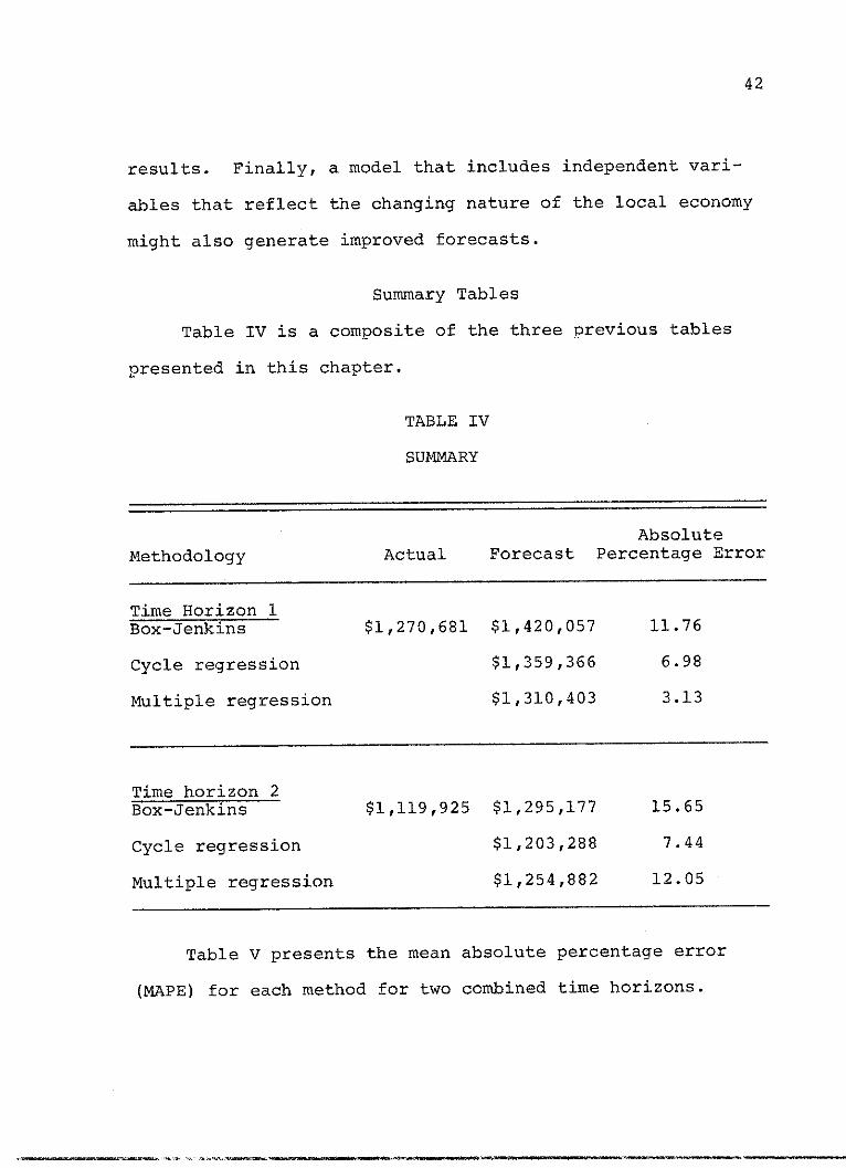
results. Finally, a model that includes independent vari-
ables that reflect the changing nature of the local economy
might also generate improved forecasts.
Summary Tables
Table IV is a composite of the three previous tables
presented in this chapter.
TABLE IV
SUMMARY
Absolute
Methodology Actual Forecast Percentage Error
Time Horizon 1Box-Jenkins $1,270,681 $1,420,057 11.76
Cycle regression $1,359,366 6.98
Multiple regression $1,310,403 3.13
Time horizon 2
Box-Jenkins $1,119,925 $1,295,177 15.65
Cycle regression $1,203,288 7.44
Multiple regression $1,254,882 12.05
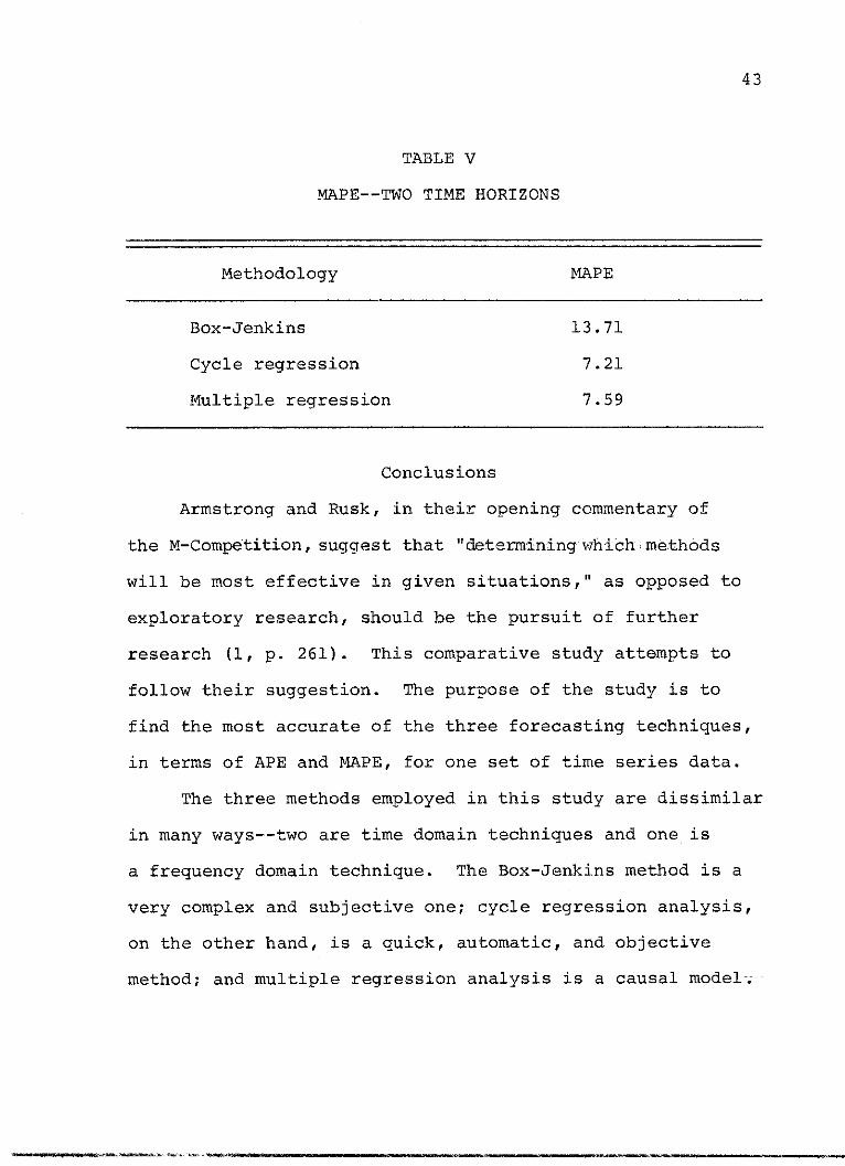
Table V presents the mean absolute percentage error
(MAPE) for each method for two combined time horizons.
43
TABLE V
MAPE--TWO TIME HORIZONS
Methodology MAPE
Box-Jenkins 13.71
Cycle regression 7.21
Multiple regression 7.59
Conclusions
Armstrong and Rusk, in their opening commentary of
the M-Competition, suggest that "determining which methods
will be most effective in given situations," as opposed to
exploratory research, should be the pursuit of further
research (1, p. 261). This comparative study attempts to
follow their suggestion. The purpose of the study is to
find the most accurate of the three forecasting techniques,
in terms of APE and MAPE, for one set of time series data.
The three methods employed in this study are dissimilar
in many ways--two are time domain techniques and one is
a frequency domain technique. The Box-Jenkins method is a
very complex and subjective one; cycle regression analysis,
on the other hand, is a quick, automatic, and objective
method; and multiple regression analysis is a causal model;

44
Yet each of these methods is a time series technique and,
as such, must address the possibility of autocorrelation
among the residuals. The various diagnostic checks were
reported throughout the study, but a warning still needs
to be included regarding autocorrelation. If it is present,
the variance of parameter estimates of a model are affected
and the precision, or significance, of those estimates can
be greatly overestimated. This does not, however, affect
the "unbiased" status of the estimates (7).
In Chapter II, the benefits of combining forecasts
werediscussed; however, this procedure does not provide
superior forecasts here because each model in this study
overestimates future revenues.
In summary, the multiple regression analysis had the
smallest APE for any method for either time horizon--3.13.
Over both time horizons, however, cycle regression analysis
was the most accurate. But, when considering which method
should be used as the best predictor of quarterly sales
tax revenues, a case by case analysis is still recommended.
In this way, the analyst can decide how factors, such as
the sophistication of the methodology, time required in
analysis, subjectivity, experience, and human intervention,
count in selecting a final forecasting model.
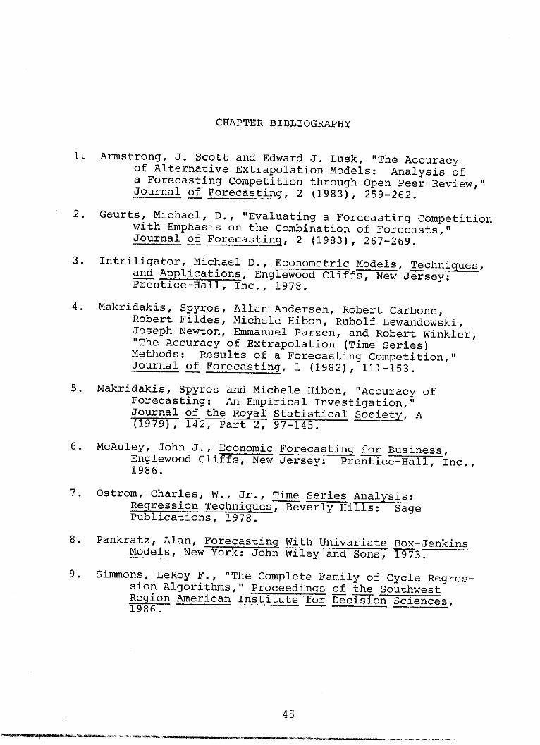
CHAPTER BIBLIOGRAPHY
1. Armstrong, J. Scott and Edward J. Lusk, "The Accuracyof Alternative Extrapolation Models: Analysis ofa Forecasting Competition through Open Peer Review,"Journal of Forecasting, 2 (1983), 259-262.
2. Geurts, Michael, D., "Evaluating a Forecasting Competitionwith Emphasis on the Combination of Forecasts,"Journal of Forecasting, 2 (1983), 267-269.
3. Intriligator, Michael D., Econometric Models, Techniques,and Applications, Englewood Cliffs, New Jersey:Prentice-Hall, Inc., 1978.
4. Makridakis, Spyros, Allan Andersen, Robert Carbone,Robert Fildes, Michele Hibon, Rubolf Lewandowski,Joseph Newton, Emmanuel Parzen, and Robert Winkler,"The Accuracy of Extrapolation (Time Series)Methods: Results of a Forecasting Competition,"Journal of Forecasting, 1 (1982), 111-153.
5. Makridakis, Spyros and Michele Hibon, "Accuracy ofForecasting: An Empirical Investigation,"Journal of the Royal Statistical Society, A(1979), 142, Part 2, 97-145.
6. McAuley, John J., Economic Forecasting for Business,Englewood Cliffs, New Jersey: Prentice-Hall, Inc.,1986.
7. Ostrom, Charles, W., Jr., Time Series Analysis:Regression Techniques, Beverly Hills: SagePublications, 1978.
8. Pankratz, Alan, Forecasting With Univariate Box-JenkinsModels, New York: John Wiley and Sons, 1973.
9. Simmons, LeRoy F., "The Complete Family of Cycle Regres-sion Algorithms, " Proceedings of the SouthwestRegion American Institute for Decision Sciences,1986.
45

APPENDIX A
46

47
QUARTERLY SALES TAX REVENUESCITY OF DENTON
Year Sales Tax Revenues
Quarter 4, 1974
1975
1976
1977
1978
1979
1980
1981
1982
238051
237199281928243754293110
281460250067335475281156
363058263610290138366233
399293370928399173460436
403093425124471492516990
552794517176629642585387
709389584962608122658992
739050627057744828704844
I z " -*-*WfflWqWWwW,

48
QUARTERLY SALES TAX REVENUES CITY OF DENTON--Continued
Year Sales Tax Revenues
1983
1984
837146755165808769900216
1062377926680
10129621074098
1304289104711611628431241014
1985
,w 'lowwooOam,

BIBLIOGRAPHY
Books
Bails, Dale G. and Larry C. Peppers, Business Fluctuations--Forecasting Techniques and Applications, EnglewoodCliffs, New Jersey: Prentice-Hall, Inc., 1982.
Gilchrist, Warren, Statistical Forecasting, New York: JohnWiley and Sons, 1976.
Intriligator, Michael D., Econometric Models, Techniques, andApplications, Englewood Cliffs, New Jersey Prentice-Hall,Inc., 1978.
Lewis-Beck, Michael S., Applied Regression An Introduction,Beverly Hills: Sage Publications, 1980.
Makridakis, Spyros, S. C. Wheelwright and V. E. McGee,Forecasting Methods and Applications, 2nd edition, NewYork: John Wiley and Sons, 1983.
McAuley, John J., Economic Forecasting for Business, EnglewoodCliffs, New Jersey: Prentice-Hall, Inc., 1986.
Ostrom, Charles, W., Jr., Time Series Analysis: RegressionTechniques, Beverly Hills: Sage Publications, 1978.
Pankratz, Alan, Forecasting With Univariate Box-JenkinsModels, New York: John Wiley and Sons, 1983.
Articles
Andersen, Allan, "Viewpoint of the Box-Jenkins Analyst in theM-Competition, " Journal of Forecasting, 2 (1983),286-287.
Armstrong, J. Scott and Edward J. Lusk, "The Accuracy ofAlternative Extrapolation Models: Analysis of aForecasting Competition through Open Peer Review,"Journal of Forecasting, 2 (1983), 259-262.
49
44

50
Geurts, Michael D., "Evaluating a Forecasting Competition withEmphasis on the Combination of Forecasts," Journal ofForecasting, 2 (1983), 267-269.
Mahmoud, Essam, "Accuracy in Forecasting: A Survey," Journalof Forecasting, 3 (1984), 139-159.
Makridakis, Spyros, Allan Andersen, Robert Carbone, RobertFildes, Michele Hibon, Rudolf Lewandowski, Joseph Newton,Emmanuel Parzen, and Robert Winkler, "The Accuracy ofExtrapolation (Time Series) Methods: Results of a Fore-casting Competition," Journal of Forecasting, 1 (1982),111-153.
Makridakis, Spyros and Michele Hibon, "Accuracy of Forecasting:An Empirical Investigation," Journal of the RoyalStatistical Society, A (1979), 142, Part 2, 97-145.
Markland, Robert E.,, "Does the M-Competition Answer the RightQuestions?," Journal of Forecasting, 2 (1983), 272-273.
Naylor, Thomas H. and T. G. Seaks, "Box-Jenkins Methods: AnAlternative to Econometric Models," InternationalStatistical Review, 40 (1972), 113-137.
Newbold, Paul, "The Competition to End All Competitions,"Journal of Forecasting, 2 (1983), 276-279.
Pack, David J., "What Do These Numbers Tell Us?," Journalof Forecasjtin, 2 (1983), 279-285.
Reeves, Gary R. and Kenneth D. Lawrence, "Combining MultipleForecasts Given Multiple Objectives," Journal of Fore-casting, 1 (1982), 271-279.
Simmons, LeRoy F., "The Complete Family of Cycle RegressionAlgorithms," Proceedings of the Southwest RegionAmerican Institute for Decision Sciences, 1986.
Simmons, LeRoy F., Mayur R. Mehta and Laurette Poulos Simmons,"Cycle Regression Analysis Made Objective--The T-ValueMethod," Cycles, 24 (1983), 99-102.

51
Simmons, LeRoy F. and Donald R. Williams, "A Cycle RegressionAnalysis Algorithm for Extracting Cycles from Time SeriesData," Journal of Computers and Operations Research, AnInternational Journal, 9 (1982), 243-254.
Simmons, LeRoy F. and Donald R. Williams, "The Use of CycleRegression Analysis to Predict Civil Violence," Journalof Interdisciplinary Cycle Research, An InternationalJournal, 14 (1983), 203-215.
Reports
Shah, Vivek, "Application of Spectral Analysis to the CycleRegression Algorithm," unpublished doctoral dissertation,North Texas State University, Denton, Texas, 1984.
W-A 0 a'" i RON 11 i I