Embed Size (px)
DESCRIPTION
Forecasting
Citation preview
Forecasting
August 29, WednesdayAugust 29, Wednesday
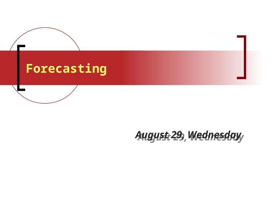
Introduction
Operations Strategy & Competitiveness
Quality Management
Strategic Decisions (some)
Design of Productsand Services
Process Selectionand Design
Capacity and Facility Decisions
Tactical & Operational Decisions
CourseStructure
Forecasting
Forecasting
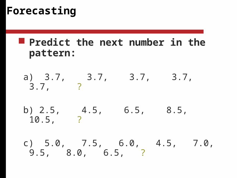
Predict the next number in the pattern:
a) 3.7, 3.7, 3.7, 3.7, 3.7, ?
b) 2.5, 4.5, 6.5, 8.5, 10.5, ?
c) 5.0, 7.5, 6.0, 4.5, 7.0, 9.5, 8.0, 6.5, ?
Forecasting
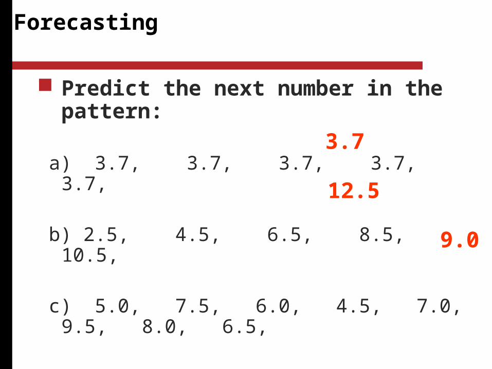
Predict the next number in the pattern:
a) 3.7, 3.7, 3.7, 3.7, 3.7,
b) 2.5, 4.5, 6.5, 8.5, 10.5,
c) 5.0, 7.5, 6.0, 4.5, 7.0, 9.5, 8.0, 6.5,
3.7
12.5
9.0
Outline
What is forecasting?
Types of forecasts Time-Series forecasting
Naïve
Moving Average
Exponential Smoothing
Regression
Good forecasts
What is Forecasting?
Process of predicting a future event based on historical data
Educated Guessing
Underlying basis of all business decisions Production Inventory Personnel Facilities
In general, forecasts are almost always wrong. So,
Why do we need to forecast?
Throughout the day we forecast very different things such as weather, traffic, stock market, state of our company from different perspectives.
Virtually every business attempt is based on forecasting. Not all of them are derived from sophisticated methods. However, “Best" educated guesses about future are more valuable for purpose of Planning than no forecasts and hence no planning.
Departments throughout the organization depend on forecasts to formulate and execute their plans.
Finance needs forecasts to project cash flows and capital requirements.
Human resources need forecasts to anticipate hiring needs.
Production needs forecasts to plan production levels, workforce, material requirements, inventories, etc.
Importance of Forecasting in OM
Demand is not the only variable of interest to forecasters.
Manufacturers also forecast worker absenteeism, machine availability, material costs, transportation and production lead times, etc.
Besides demand, service providers are also interested in forecasts of population, of other demographic variables, of weather, etc.
Importance of Forecasting in OM
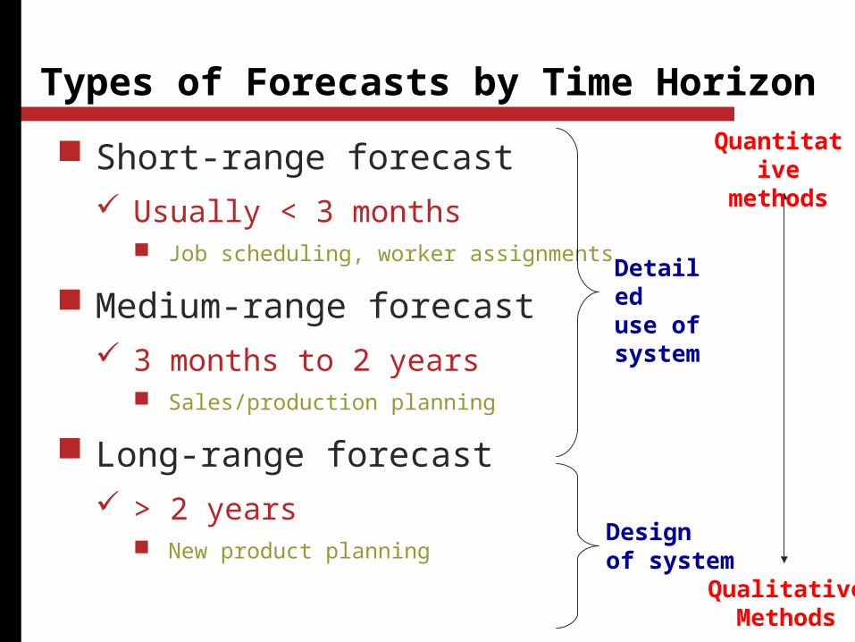
Short-range forecast Usually < 3 months
Job scheduling, worker assignments
Medium-range forecast 3 months to 2 years
Sales/production planning
Long-range forecast > 2 years
New product planning
Types of Forecasts by Time Horizon
Designof system
Detailed use ofsystem
Quantitative
methods
QualitativeMethods
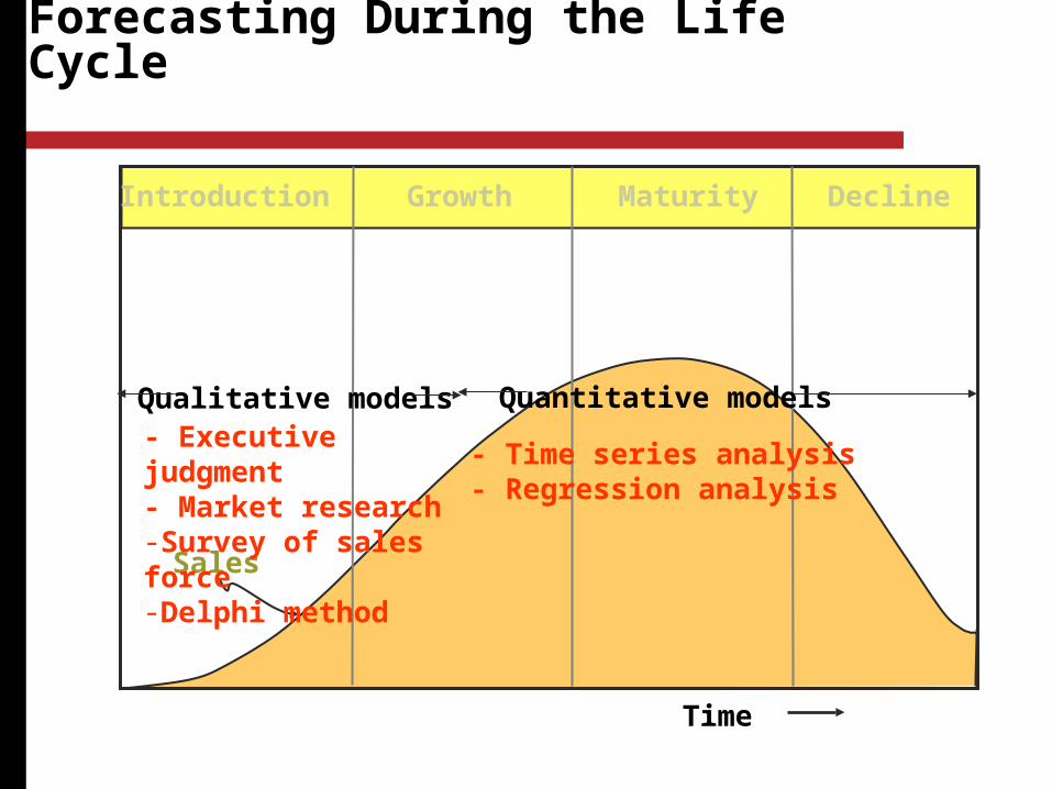
Forecasting During the Life Cycle
Introduction Growth Maturity Decline
Sales
Time
Quantitative models
- Time series analysis- Regression analysis
Qualitative models- Executive judgment- Market research-Survey of sales force-Delphi method
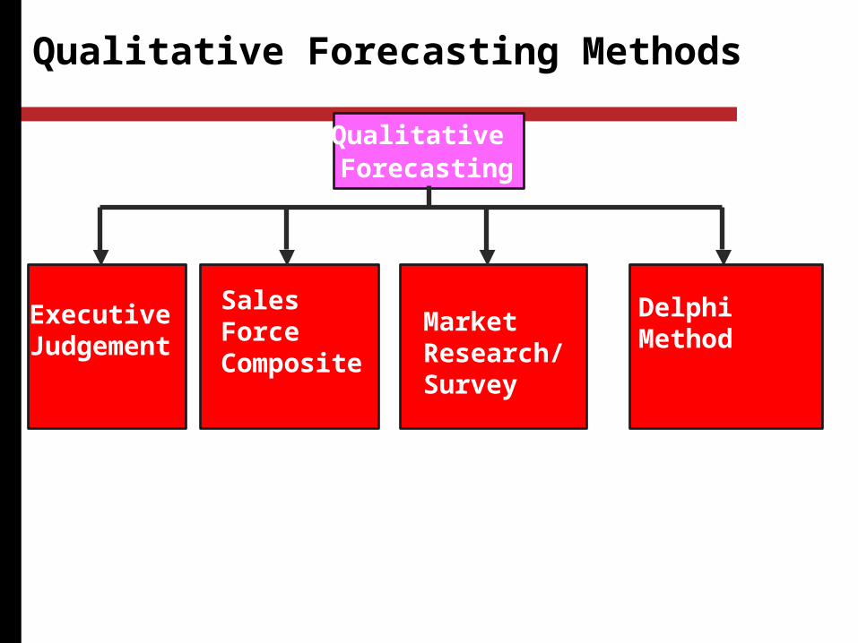
Qualitative Forecasting Methods
QualitativeForecasting
ModelsMarketResearch/Survey
SalesForceComposite
Executive Judgement
DelphiMethod
Smoothing
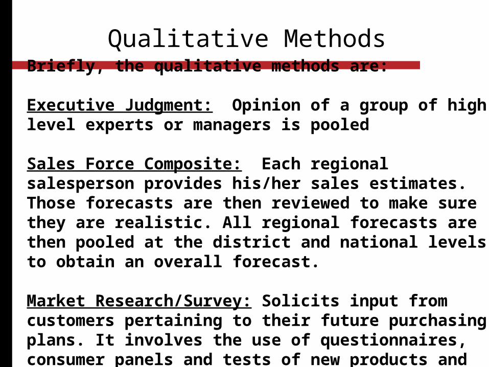
Briefly, the qualitative methods are:
Executive Judgment: Opinion of a group of high level experts or managers is pooled
Sales Force Composite: Each regional salesperson provides his/her sales estimates. Those forecasts are then reviewed to make sure they are realistic. All regional forecasts are then pooled at the district and national levels to obtain an overall forecast.
Market Research/Survey: Solicits input from customers pertaining to their future purchasing plans. It involves the use of questionnaires, consumer panels and tests of new products and services.
.
Qualitative Methods
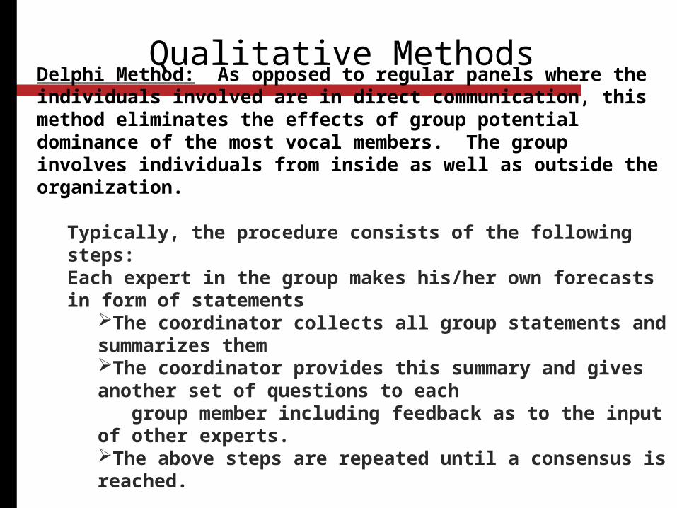
Delphi Method: As opposed to regular panels where the individuals involved are in direct communication, this method eliminates the effects of group potential dominance of the most vocal members. The group involves individuals from inside as well as outside the organization.
Typically, the procedure consists of the following steps:Each expert in the group makes his/her own forecasts in form of statements
The coordinator collects all group statements and summarizes themThe coordinator provides this summary and gives another set of questions to each group member including feedback as to the input of other experts.The above steps are repeated until a consensus is reached.
.
Qualitative Methods
Quantitative Forecasting Methods
QuantitativeForecasting
RegressionModels
2. MovingAverage
1. Naive
Time SeriesModels
3. ExponentialSmoothing
a) simpleb) weighted
a) levelb) trendc) seasonality
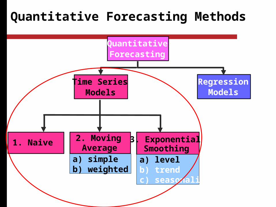
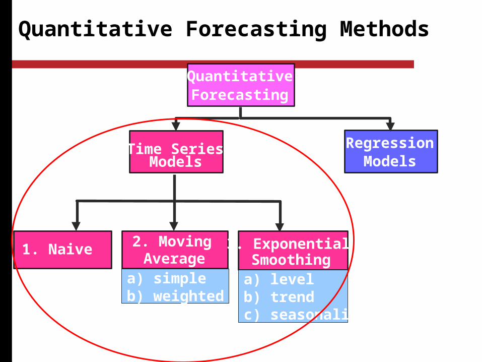
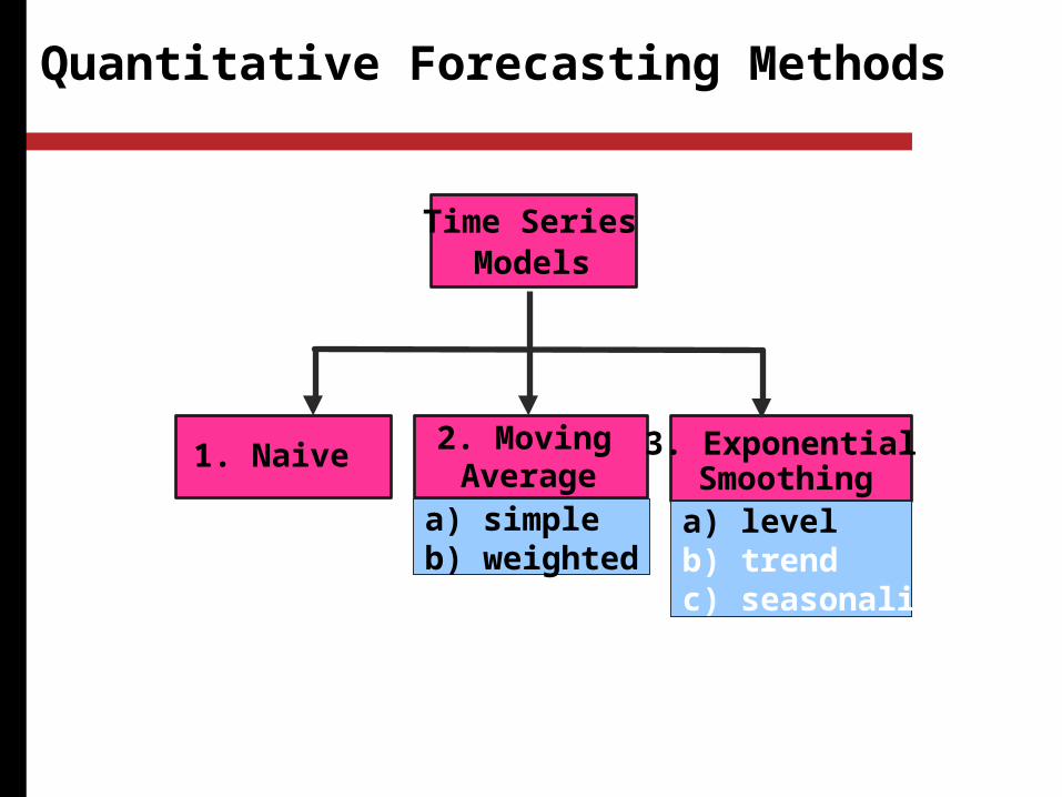
Quantitative Forecasting Methods
QuantitativeForecasting
RegressionModels
2. MovingAverage
1. Naive
Time SeriesModels
3. ExponentialSmoothing
a) simpleb) weighted
a) levelb) trendc) seasonality
Time Series Models
Try to predict the future based on past data
Assume that factors influencing the past will continue to influence the future
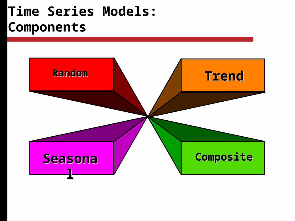
RandomRandom
SeasonalSeasonal
TrendTrend
CompositeComposite
Time Series Models: Components
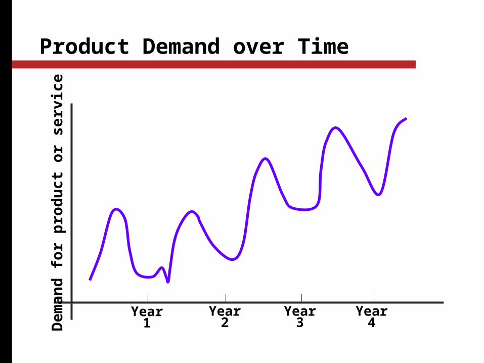
Product Demand over Time
Year1
Year2
Year3
Year4
Dem
and
for p
rodu
ct o
r ser
vice

Product Demand over Time
Year1
Year2
Year3
Year4
Dem
and
for p
rodu
ct o
r ser
vice
Trend component
Actual demand line
Seasonal peaks
Random variation
Now let’s look at some time series approaches to forecasting…Borrowed from Heizer/Render - Principles of Operations Management, 5e, and Operations Management, 7e
Quantitative Forecasting Methods
Quantitative
Models
2. MovingAverage
1. Naive
Time SeriesModels
3. ExponentialSmoothing
a) simpleb) weighted
a) levelb) trendc) seasonality
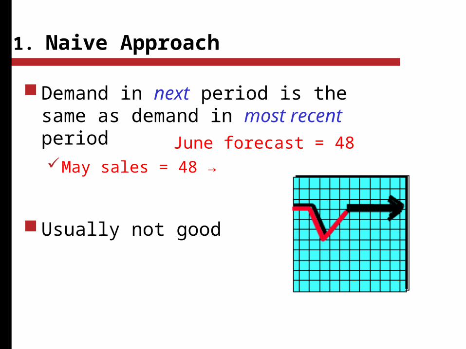
1. Naive Approach
Demand in next period is the same as demand in most recent periodMay sales = 48 →
Usually not good
June forecast = 48
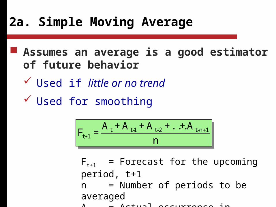
2a. Simple Moving Average
n
A+...+A +A +A =F 1n-t2-t1-tt
1t
n
A+...+A +A +A =F 1n-t2-t1-tt
1t
Assumes an average is a good estimator of future behavior
Used if little or no trend
Used for smoothing
Ft+1 = Forecast for the upcoming period, t+1n = Number of periods to be averagedA t = Actual occurrence in period t
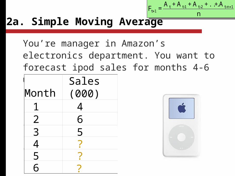
2a. Simple Moving Average
You’re manager in Amazon’s electronics department. You want to forecast ipod sales for months 4-6 using a 3-period moving average.
n
A+...+A +A +A =F 1n-t2-t1-tt
1t
n
A+...+A +A +A =F 1n-t2-t1-tt
1t
MonthSales(000)
1 42 63 54 ?5 ?6 ?
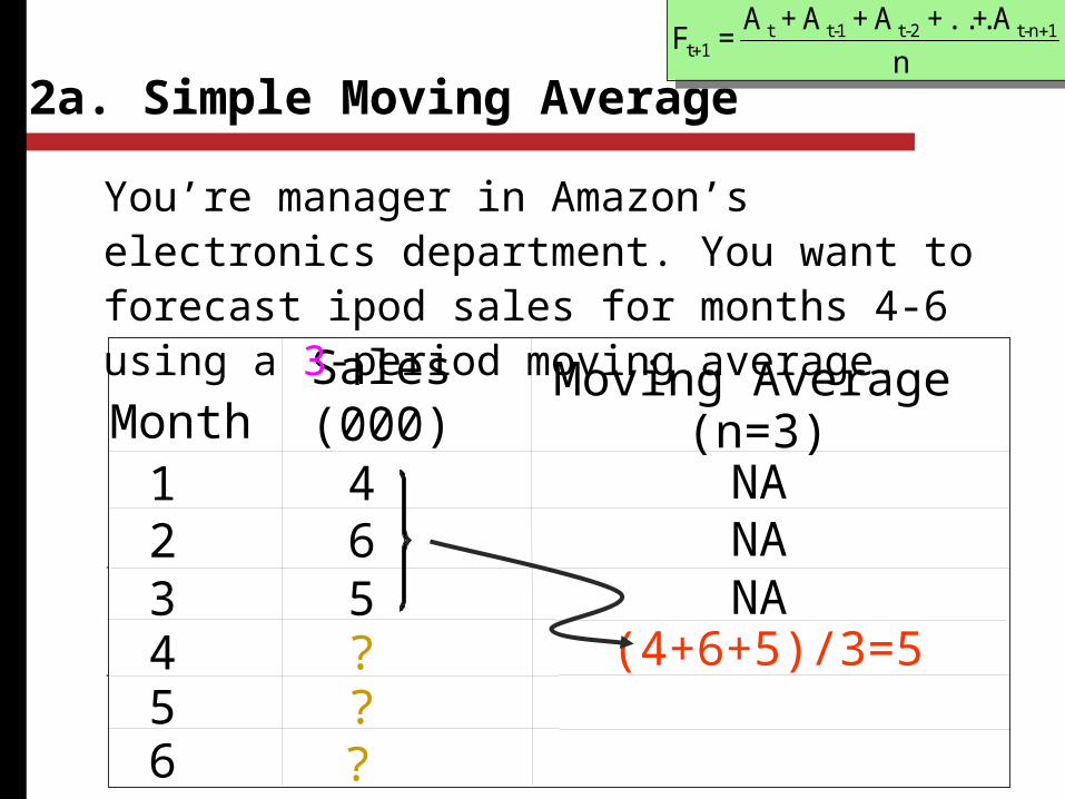
2a. Simple Moving Average
MonthSales(000)
Moving Average(n=3)
1 4 NA2 6 NA3 5 NA4 ?5 ?
(4+6+5)/3=5
6 ?
n
A+...+A +A +A =F 1n-t2-t1-tt
1t
n
A+...+A +A +A =F 1n-t2-t1-tt
1t
You’re manager in Amazon’s electronics department. You want to forecast ipod sales for months 4-6 using a 3-period moving average.
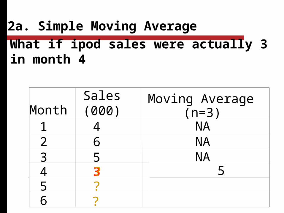
What if ipod sales were actually 3 in month 4
MonthSales(000)
Moving Average(n=3)
1 4 NA2 6 NA3 5 NA4 35 ?
5
6 ?
2a. Simple Moving Average
?
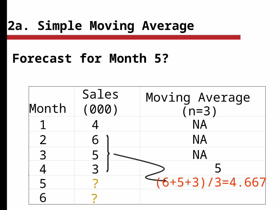
Forecast for Month 5?
MonthSales(000)
Moving Average(n=3)
1 4 NA2 6 NA3 5 NA4 35 ?
5
6 ?(6+5+3)/3=4.667
2a. Simple Moving Average
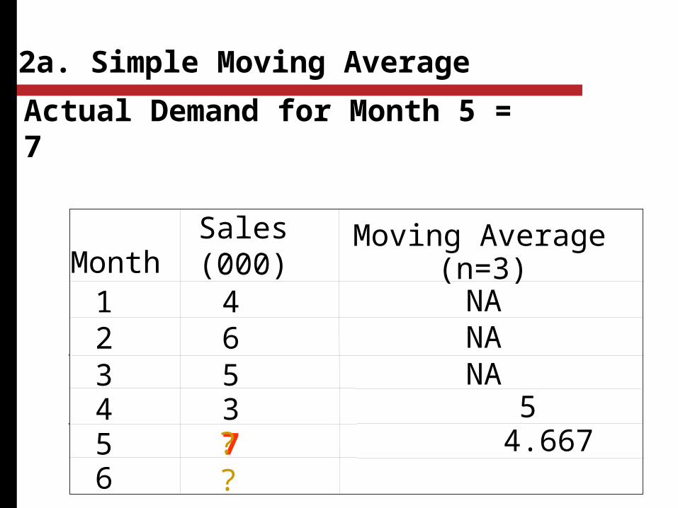
Actual Demand for Month 5 = 7
MonthSales(000)
Moving Average(n=3)
1 4 NA2 6 NA3 5 NA4 35 7
5
6 ? 4.667
2a. Simple Moving Average
?
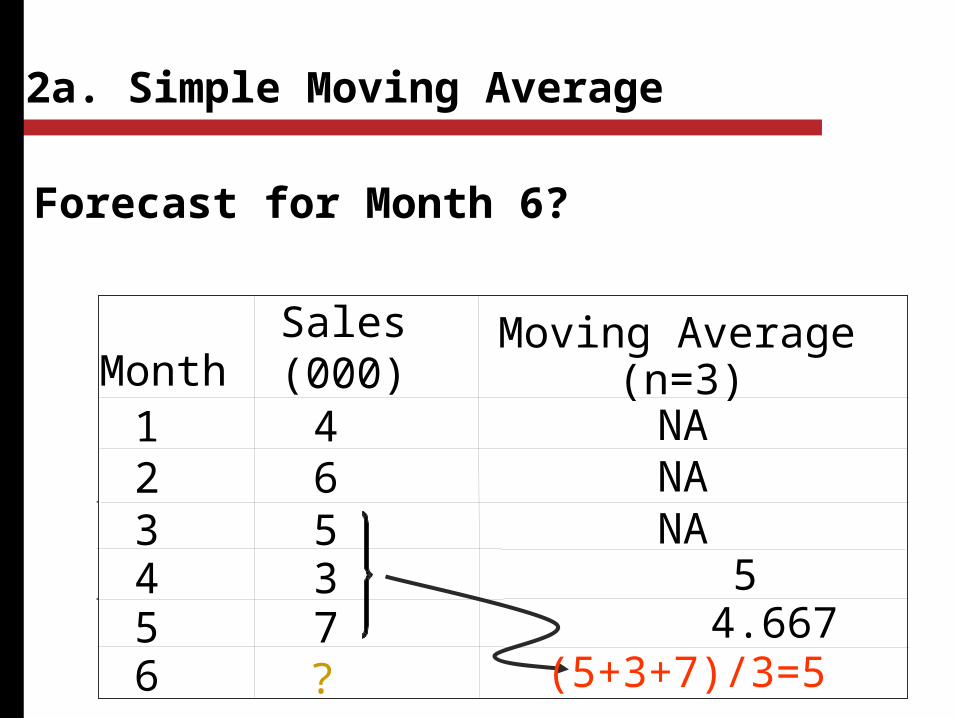
Forecast for Month 6?
MonthSales(000)
Moving Average(n=3)
1 4 NA2 6 NA3 5 NA4 35 7
5
6 ? 4.667(5+3+7)/3=5
2a. Simple Moving Average
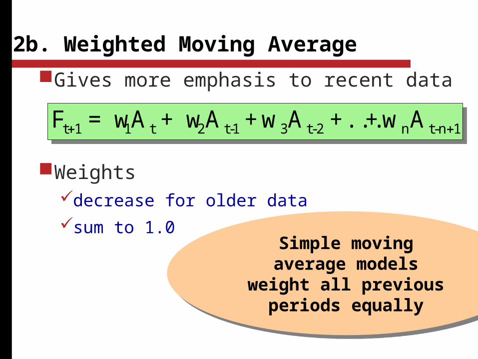
Gives more emphasis to recent data
Weights decrease for older data
sum to 1.0
2b. Weighted Moving Average
1n-tn2-t31-t2t11t Aw+...+Aw+A w+A w=F 1n-tn2-t31-t2t11t Aw+...+Aw+A w+A w=F
Simple movingaverage models
weight all previousperiods equally
Simple movingaverage models
weight all previousperiods equally
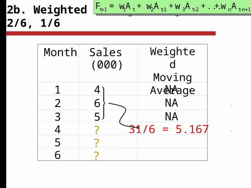
2b. Weighted Moving Average: 3/6, 2/6, 1/6
Month WeightedMoving Average
1 4 NA2 6 NA3 5 NA4 31/6 = 5.16756 ?
??
1n-tn2-t31-t2t11t Aw+...+Aw+A w+A w=F 1n-tn2-t31-t2t11t Aw+...+Aw+A w+A w=F
Sales(000)
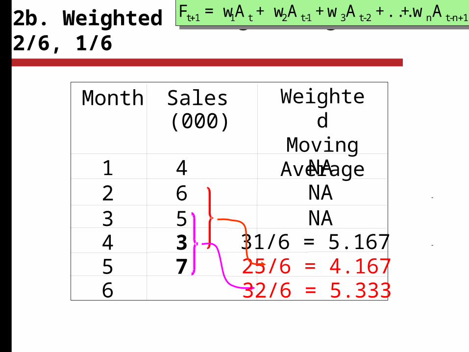
2b. Weighted Moving Average: 3/6, 2/6, 1/6
Month Sales(000)
WeightedMoving Average
1 4 NA2 6 NA3 5 NA4 3 31/6 = 5.1675 76
25/6 = 4.16732/6 = 5.333
1n-tn2-t31-t2t11t Aw+...+Aw+A w+A w=F 1n-tn2-t31-t2t11t Aw+...+Aw+A w+A w=F
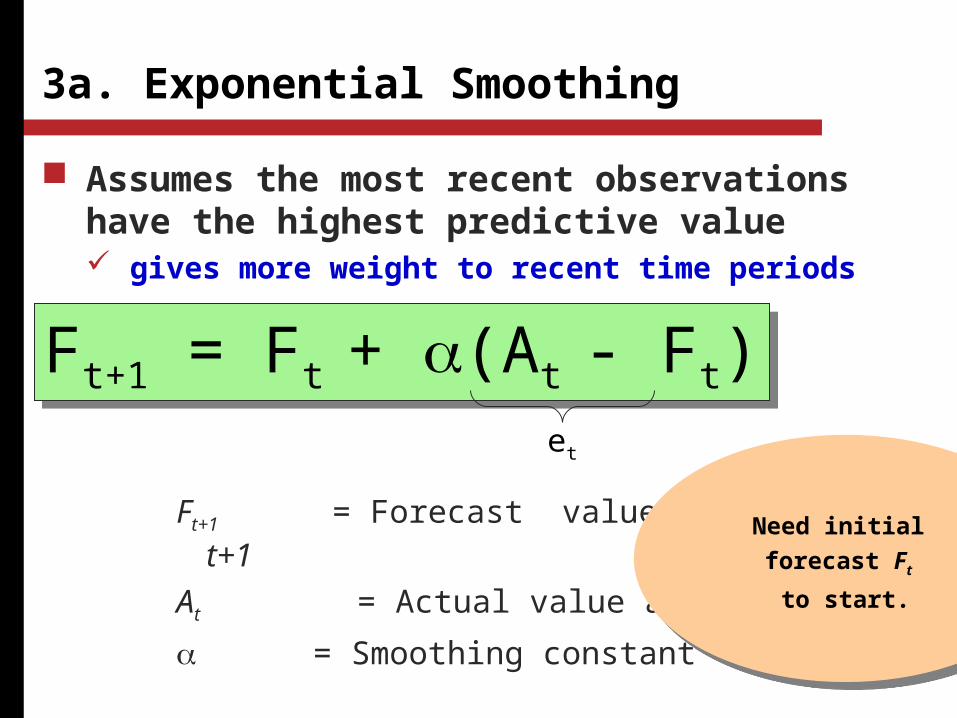
3a. Exponential Smoothing
Assumes the most recent observations have the highest predictive value gives more weight to recent time periods
Ft+1 = Ft + (At - Ft)Ft+1 = Ft + (At - Ft)et
Ft+1 = Forecast value for time t+1
At = Actual value at time t
= Smoothing constant
Need initial
forecast Ft
to start.
Need initial
forecast Ft
to start.
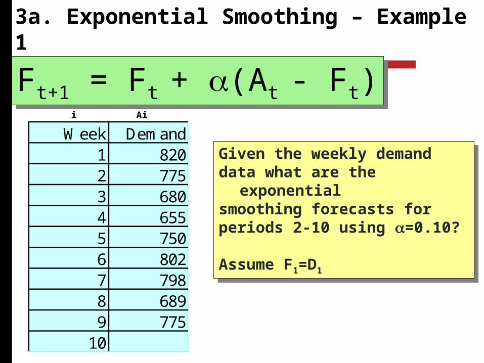
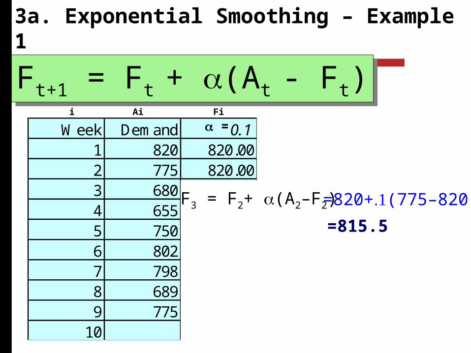
3a. Exponential Smoothing – Example 1
Week Demand1 8202 7753 6804 6555 7506 8027 7988 6899 775
10
Given the weekly demand data what are the exponentialsmoothing forecasts for periods 2-10 using =0.10?
Assume F1=D1
Given the weekly demand data what are the exponentialsmoothing forecasts for periods 2-10 using =0.10?
Assume F1=D1
Ft+1 = Ft + (At - Ft)Ft+1 = Ft + (At - Ft)i Ai
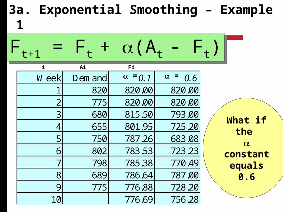
Week Demand 0.1 0.61 820 820.00 820.002 775 820.00 820.003 680 815.50 793.004 655 801.95 725.205 750 787.26 683.086 802 783.53 723.237 798 785.38 770.498 689 786.64 787.009 775 776.88 728.20
10 776.69 756.28
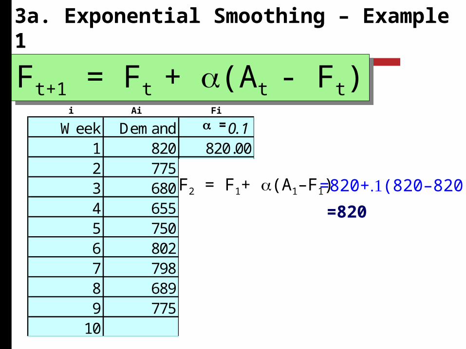
Ft+1 = Ft + (At - Ft)Ft+1 = Ft + (At - Ft)3a. Exponential Smoothing – Example 1
=
F2 = F1+ (A1–F1) =820+(820–820)
=820
i Ai Fi
Week Demand 0.1 0.61 820 820.00 820.002 775 820.00 820.003 680 815.50 793.004 655 801.95 725.205 750 787.26 683.086 802 783.53 723.237 798 785.38 770.498 689 786.64 787.009 775 776.88 728.20
10 776.69 756.28
Ft+1 = Ft + (At - Ft)Ft+1 = Ft + (At - Ft)3a. Exponential Smoothing – Example 1
=
F3 = F2+ (A2–F2) =820+(775–820)
=815.5
i Ai Fi
Week Demand 0.1 0.61 820 820.00 820.002 775 820.00 820.003 680 815.50 793.004 655 801.95 725.205 750 787.26 683.086 802 783.53 723.237 798 785.38 770.498 689 786.64 787.009 775 776.88 728.20
10 776.69 756.28
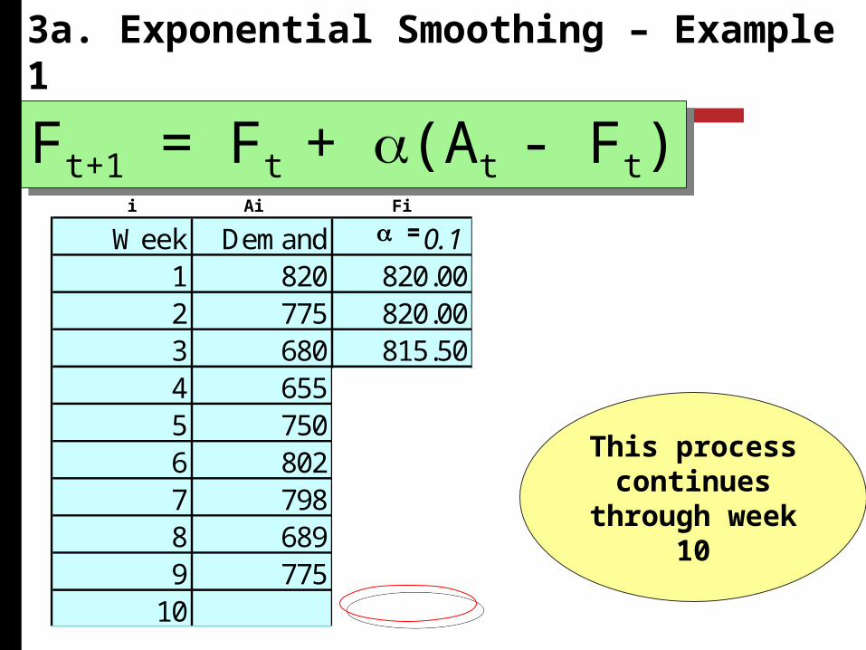
Ft+1 = Ft + (At - Ft)Ft+1 = Ft + (At - Ft)
This process continues
through week 10
3a. Exponential Smoothing – Example 1
=i Ai Fi
Week Demand 0.1 0.61 820 820.00 820.002 775 820.00 820.003 680 815.50 793.004 655 801.95 725.205 750 787.26 683.086 802 783.53 723.237 798 785.38 770.498 689 786.64 787.009 775 776.88 728.20
10 776.69 756.28
Ft+1 = Ft + (At - Ft)Ft+1 = Ft + (At - Ft)
What if the constant equals 0.6
3a. Exponential Smoothing – Example 1
= =i Ai Fi
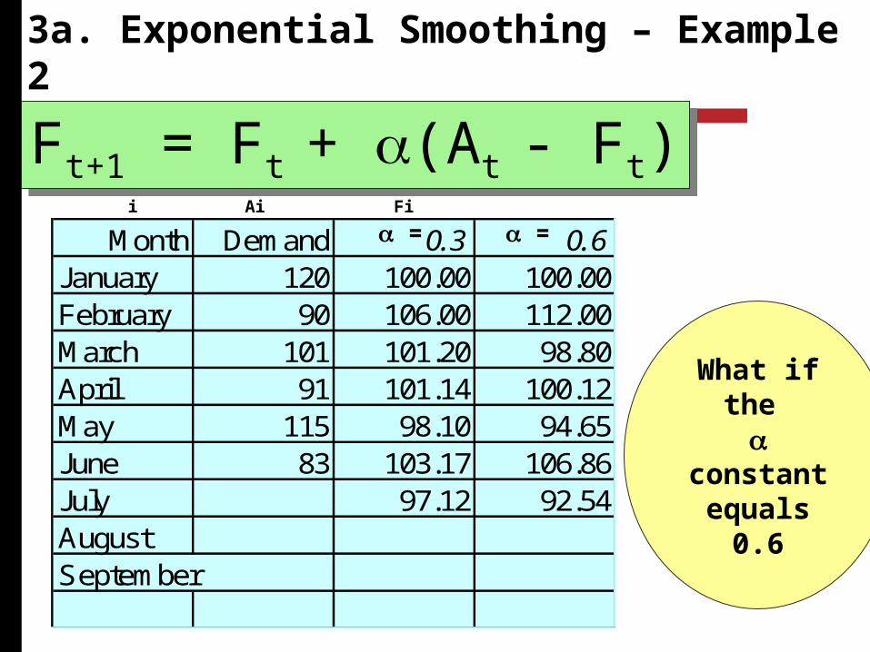
Month Demand 0.3 0.6January 120 100.00 100.00February 90 106.00 112.00March 101 101.20 98.80April 91 101.14 100.12May 115 98.10 94.65June 83 103.17 106.86July 97.12 92.54AugustSeptember
Ft+1 = Ft + (At - Ft)Ft+1 = Ft + (At - Ft)
What if the constant equals 0.6
3a. Exponential Smoothing – Example 2
= =i Ai Fi
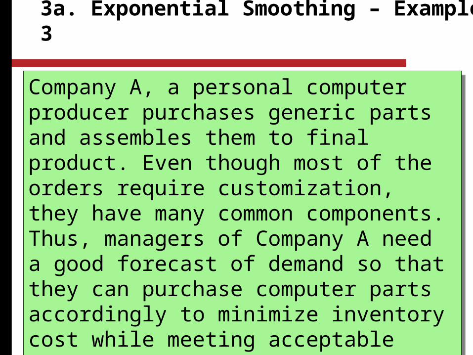
Company A, a personal computer producer purchases generic parts and assembles them to final product. Even though most of the orders require customization, they have many common components. Thus, managers of Company A need a good forecast of demand so that they can purchase computer parts accordingly to minimize inventory cost while meeting acceptable service level. Demand data for its computers for the past 5
months is given in the following table.
3a. Exponential Smoothing – Example 3

Month Demand 0.3 0.5January 80 84.00 84.00February 84 82.80 82.00March 82 83.16 83.00April 85 82.81 82.50May 89 83.47 83.75June 85.13 86.38July ?? ??
Ft+1 = Ft + (At - Ft)Ft+1 = Ft + (At - Ft)
What if the constant equals 0.5
3a. Exponential Smoothing – Example 3
= =i Ai Fi
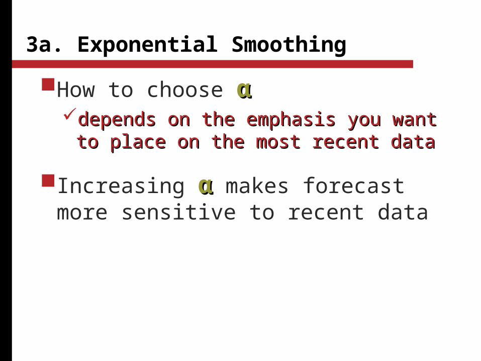
How to choose ααdepends on the emphasis you want to place depends on the emphasis you want to place
on the most recent dataon the most recent data
Increasing αα makes forecast more sensitive to recent data
3a. Exponential Smoothing
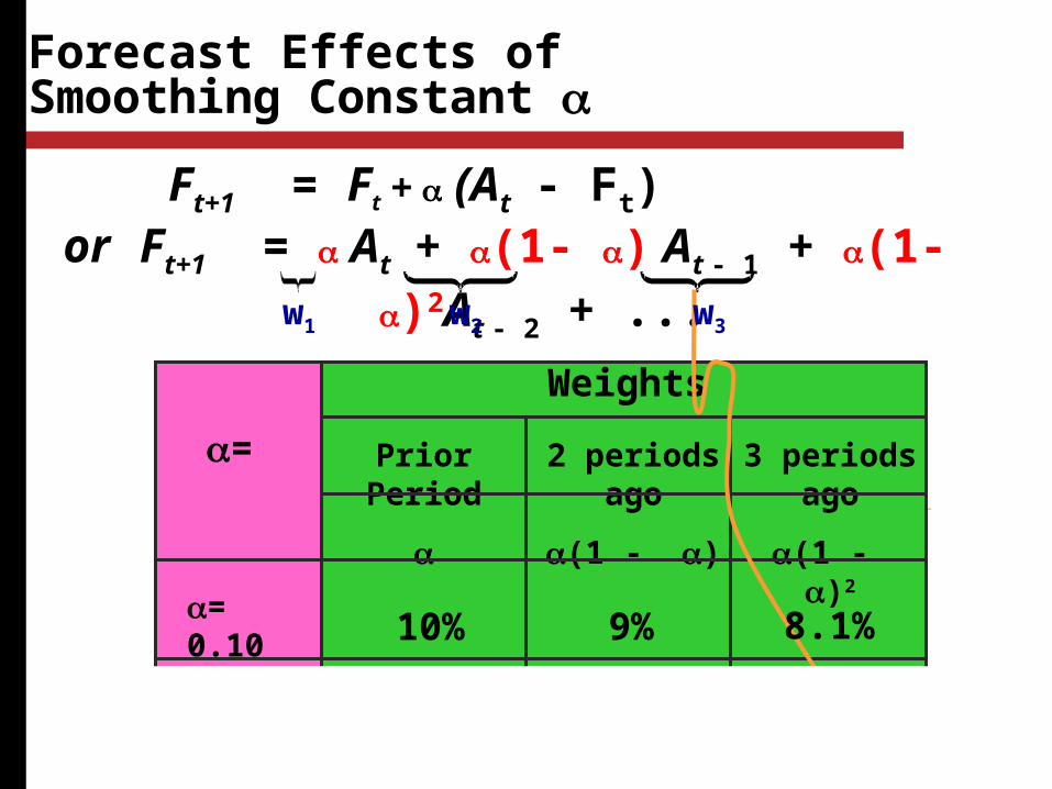
Ft+1 = At + (1- ) At - 1 + (1- )2At - 2 + ...
Forecast Effects ofSmoothing Constant
Weights
Prior Period
2 periods ago
(1 - )
3 periods ago
(1 - )2
=
= 0.10
= 0.90
10% 9% 8.1%
90% 9% 0.9%
Ft+1 = Ft + (At - Ft)or
w1 w2 w3

Collect historical data
Select a model Moving average methods
Select n (number of periods) For weighted moving average: select weights
Exponential smoothing Select
Selections should produce a good forecast
To Use a Forecasting Method
…but what is a good forecast?
A Good Forecast
Has a small error Error = Demand - Forecast
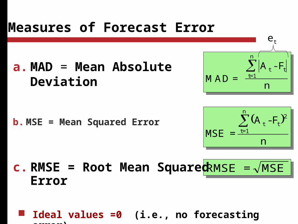
Measures of Forecast Error
b. MSE = Mean Squared Error
n
F-A =MSE
n
1=t
2tt
n
F-A =MSE
n
1=t
2tt
MAD = A - F
n
t tt=1
n
MAD =
A - F
n
t tt=1
n
et
Ideal values =0 (i.e., no forecasting error)
MSE =RMSE MSE =RMSEc. RMSE = Root Mean Squared Error
a. MAD = Mean Absolute Deviation
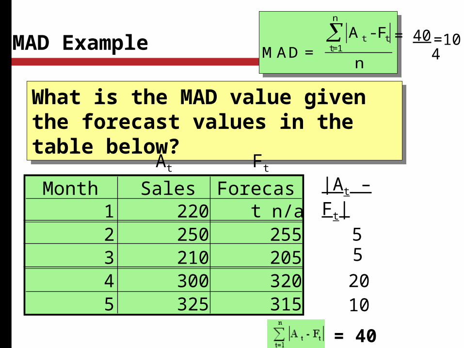
MAD Example
Month Sales Forecast1 220 n/a2 250 2553 210 2054 300 3205 325 315
What is the MAD value given the forecast values in the table below?
What is the MAD value given the forecast values in the table below?
MAD = A - F
n
t tt=1
n
MAD =
A - F
n
t tt=1
n
55
2010
|At – Ft|FtAt
= 40
= 40 4
=10
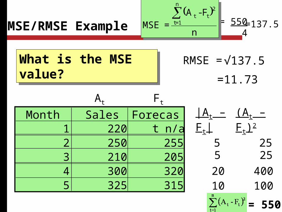
MSE/RMSE Example
Month Sales Forecast1 220 n/a2 250 2553 210 2054 300 3205 325 315
What is the MSE value?What is the MSE value?
55
2010
|At – Ft|FtAt
= 550 4
=137.5
(At – Ft)2
2525
400100
= 550
n
F-A =MSE
n
1=t
2tt
n
F-A =MSE
n
1=t
2tt
RMSE = √137.5
=11.73
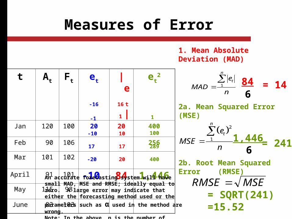
Measures of Error
t At Ft et |et| et2
Jan 120 100 20 20 400
Feb 90 106 256
Mar 101 102
April 91 101
May 115 98
June 83 103
1. Mean Absolute Deviation (MAD)
n
eMAD
n
t 1
2a. Mean Squared Error (MSE)
MSE
e
n
t
n
2
1
2b. Root Mean Squared Error (RMSE)
RMSE MSE
-16 16
-1 1
-10
17
-20
10
17
20
1
100
289
400
-10 84 1,446
846
= 14
1,4466
= 241
= SQRT(241)=15.52
An accurate forecasting system will have small MAD, MSE and RMSE; ideally equal to zero. A large error may indicate that either the forecasting method used or the
parameters such as α used in the method are wrong. Note: In the above, n is the number of periods, which is 6 in our example
deviation absoluteMean
)(=
MAD
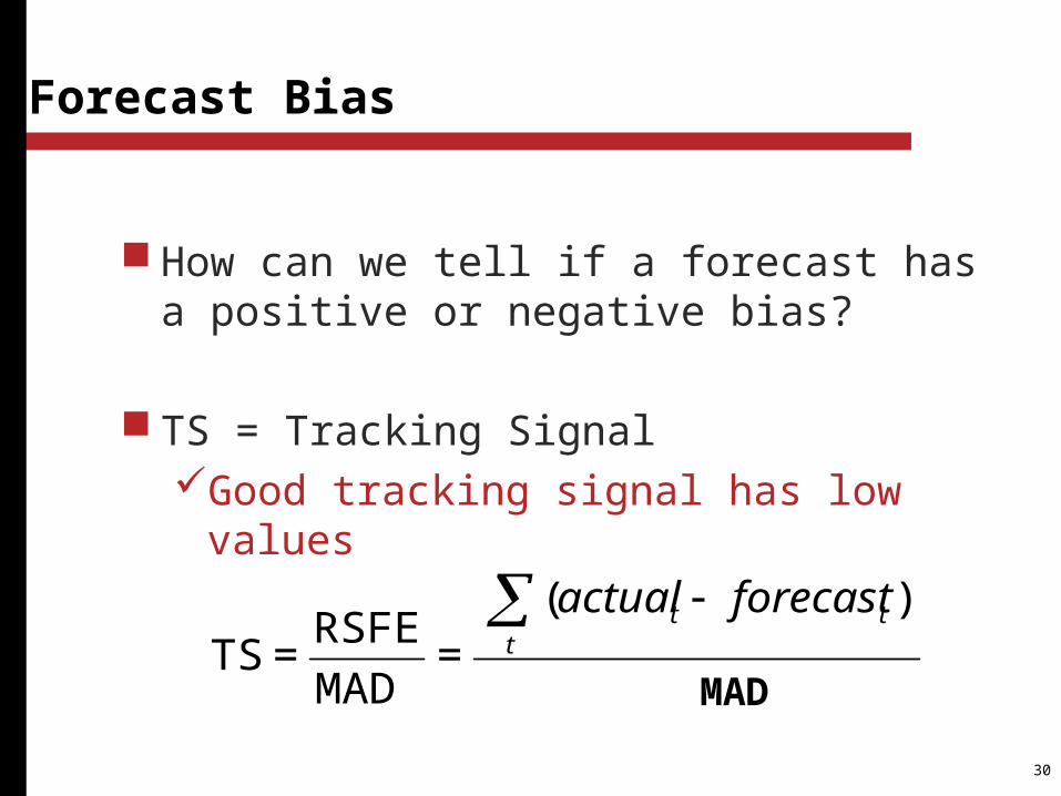
RSFE=TS
t
tt forecastactual
30
How can we tell if a forecast has a positive or negative bias?
TS = Tracking Signal Good tracking signal has low values
Forecast Bias
MAD
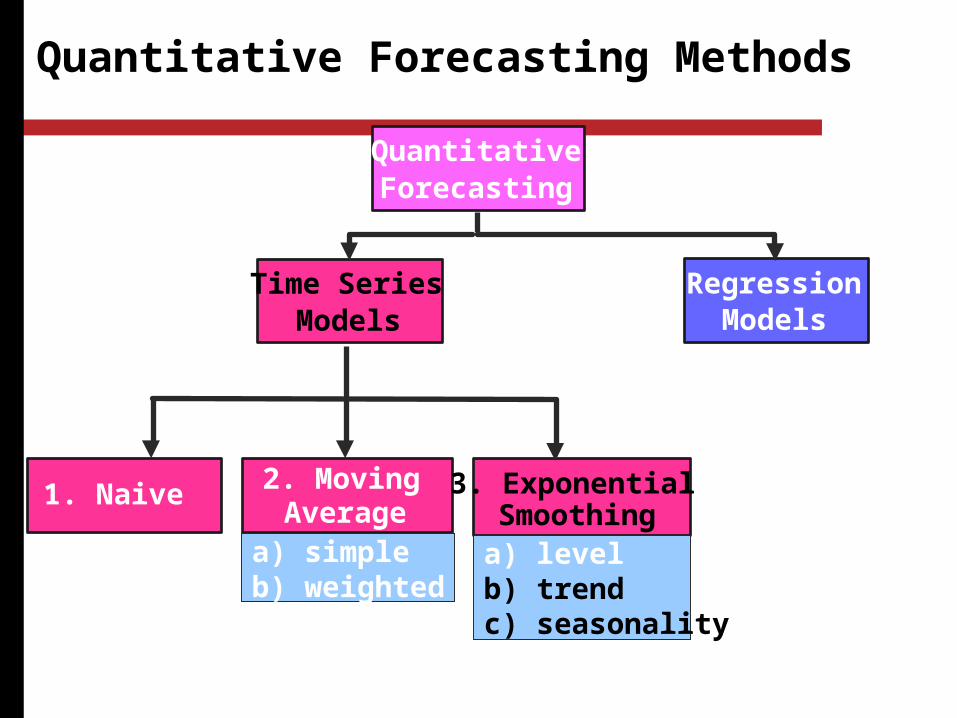
Quantitative Forecasting Methods
QuantitativeForecasting
RegressionModels
2. MovingAverage
1. Naive
Time SeriesModels
3. ExponentialSmoothing
a) simpleb) weighted
a) levelb) trendc) seasonality
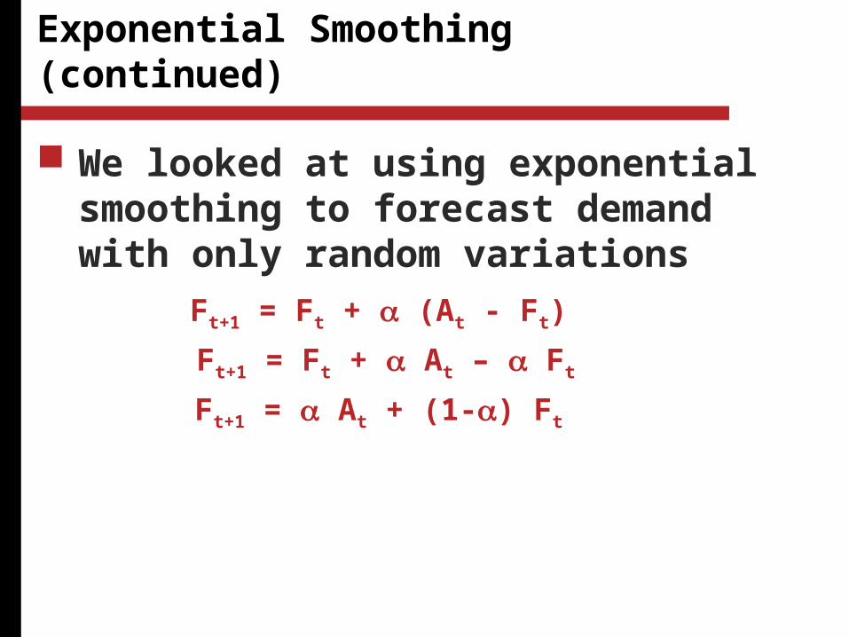
We looked at using exponential smoothing to forecast demand with only random variations
Exponential Smoothing (continued)
Ft+1 = Ft + (At - Ft)
Ft+1 = Ft + At – Ft
Ft+1 = At + (1-) Ft
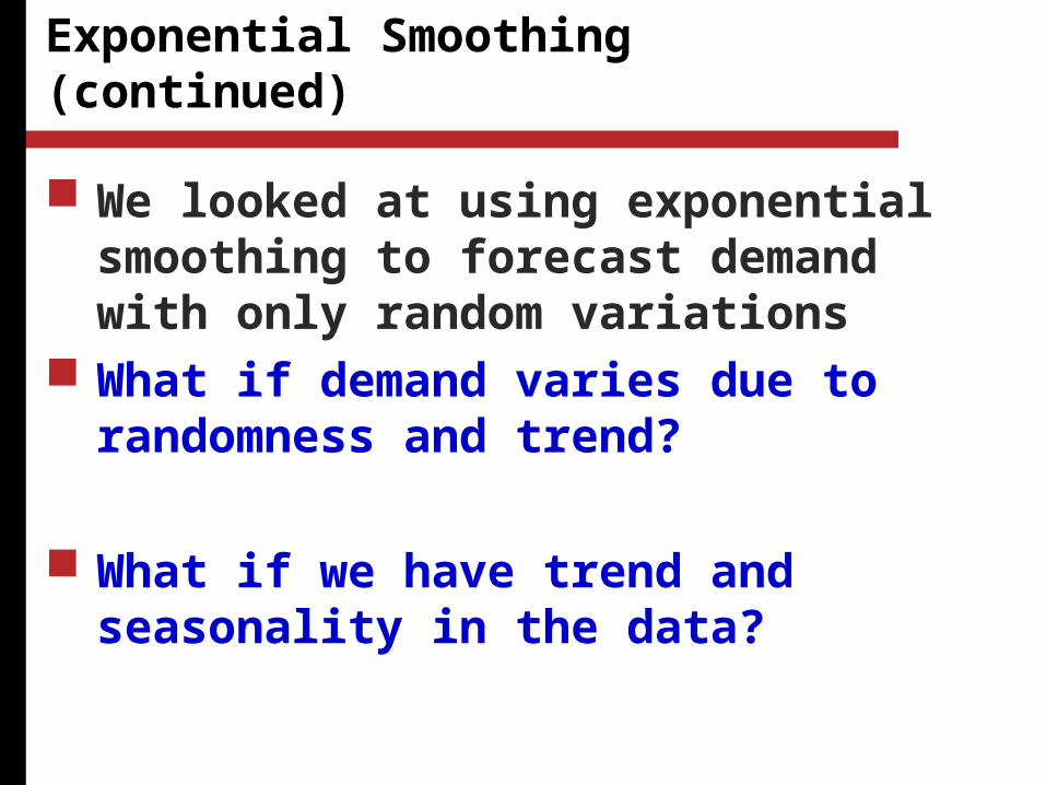
Exponential Smoothing (continued)
We looked at using exponential smoothing to forecast demand with only random variations
What if demand varies due to randomness and trend?
What if we have trend and seasonality in the data?
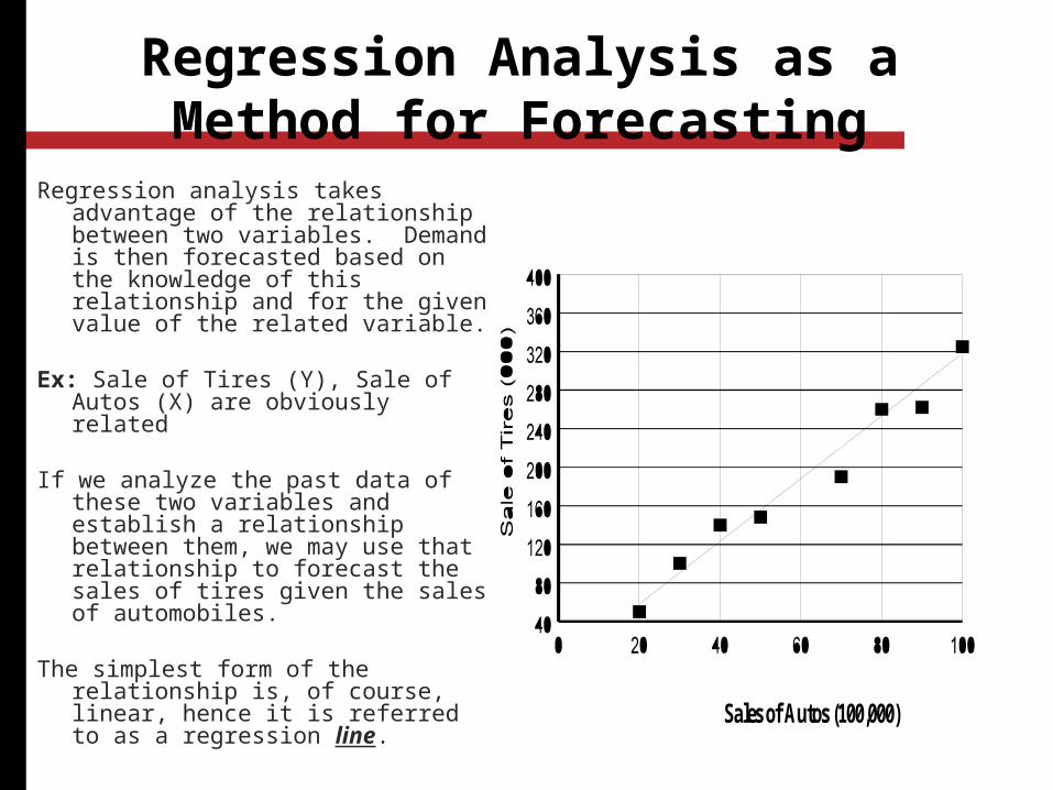
Regression Analysis as a Method for Forecasting
Regression analysis takes advantage of the relationship between two variables. Demand is then forecasted based on the knowledge of this relationship and for the given value of the related variable.
Ex: Sale of Tires (Y), Sale of Autos (X) are obviously related
If we analyze the past data of these two variables and establish a relationship between them, we may use that relationship to forecast the sales of tires given the sales of automobiles.
The simplest form of the relationship is, of course, linear, hence it is referred to as a regression line.
Sales of Autos (100,000)

Formulas
xbya
22 xnx
yxnxyb
x
y
xy
y = a + b x
where,
y = a + b x
where,
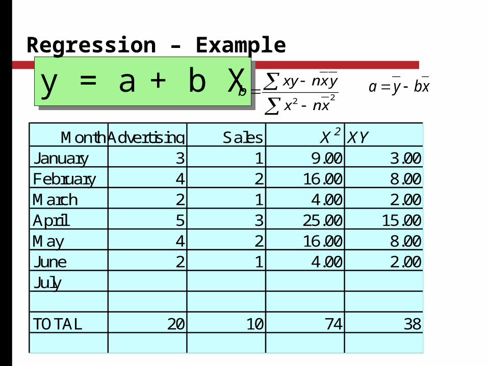
MonthAdvertising Sales X2 XYJanuary 3 1 9.00 3.00February 4 2 16.00 8.00March 2 1 4.00 2.00April 5 3 25.00 15.00May 4 2 16.00 8.00June 2 1 4.00 2.00July
TOTAL 20 10 74 38
y = a + b Xy = a + b X Regression – Example
22 xnx
yxnxyb xbya
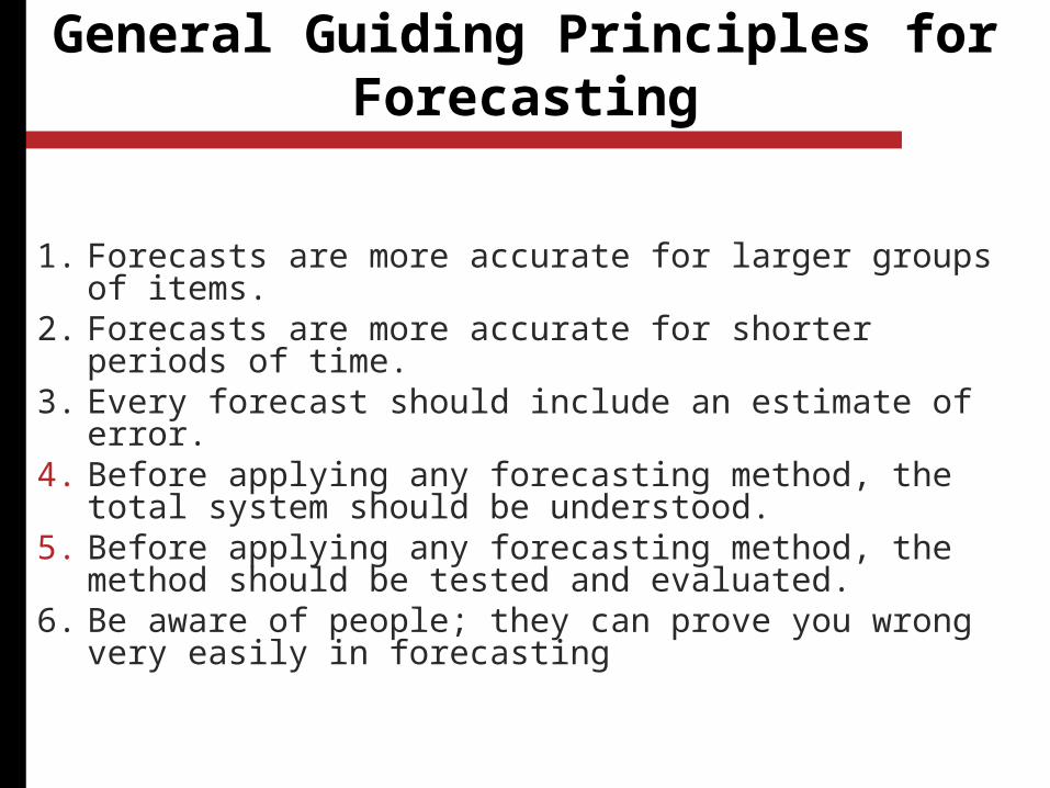
General Guiding Principles for Forecasting
1. Forecasts are more accurate for larger groups of items. 2. Forecasts are more accurate for shorter periods of time.3. Every forecast should include an estimate of error.4. Before applying any forecasting method, the total system
should be understood.5. Before applying any forecasting method, the method should
be tested and evaluated.6. Be aware of people; they can prove you wrong very easily
in forecasting
FOR JULY 2nd MONDAY
READ THE CHAPTERS ON Forecasting Product and service design