Embed Size (px)
Citation preview

Shabani, Mimoza (2015) The incidence of bank default and capital adequacy regulation in U.S. and Japan. PhD Thesis. SOAS, University of London. http://eprints.soas.ac.uk/id/eprint/20381
Copyright © and Moral Rights for this PhD Thesis are retained by the author and/or
other copyright owners.
A copy can be downloaded for personal non‐commercial research or study, without prior
permission or charge.
This PhD Thesis cannot be reproduced or quoted extensively from without first
obtaining permission in writing from the copyright holder/s.
The content must not be changed in any way or sold commercially in any format or
medium without the formal permission of the copyright holders.
When referring to this PhD Thesis, full bibliographic details including the author, title,
awarding institution and date of the PhD Thesis must be given e.g. AUTHOR (year of
submission) "Full PhD Thesis title", name of the School or Department, PhD PhD Thesis,
pagination.
The Incidence of Bank Default and
Capital Adequacy Regulation in U.S.
and Japan
Mimoza Shabani
Thesis submitted for the degree of PhD
September 2014
Department of Economics
SOAS, University of London

2
Declaration for SOAS PhD thesis I have read and understood regulation 17.9 of the Regulations for students of the SOAS, University of London concerning plagiarism. I undertake that all the material presented for examination is my own work and has not been written for me, in whole or in part, by any other person. I also undertake that any quotation or paraphrase from the published or unpublished work of another person has been duly acknowledged in the work which I present for examination. Signed: Mimoza Shabani_______ Date: _September 2014________________

3
Acknowledgements
I am grateful to SOAS for awarding me a Doctoral Scholarship to undertake this
research.
I am greatly indebted to my supervisor Prof. Jan Toporowski for his support, guidance
and patience over these last four years. I am also very grateful to Prof. Gary Dymski
and Prof. Shigeyuki Hattori for their comments and feedback. I would like to express
my gratitude to Dr. Graham Smith and Dr. George Kavetsos for the feedback and
suggestions on the empirical work undertaken in this thesis. Also, I would like to
acknowledge the valuable suggestions I received during my viva examination from
Prof. Ray Barrell. Some of these suggestions have been added into the analysis of this
thesis as part of the minor revisions procedure.
I owe much gratitude to a number of fellow colleagues at SOAS. Our discussions
have helped me in so many ways. Special thanks go to Osiel Gonzales Davila and Ina
Qefalia for the time and the valuable comments they gave me.
I am very thankful for the unconditional love and support from my family. In
particular I would like to express my deepest gratitude to my parents for their love,
support and for always putting me first. My siblings, Edvin and Erida Shabani, you
know what you have done for me. Thank you! To my beautiful niece Noemi for just
being wonderful.
To the love of my life, Leni, for understanding, encouraging and supporting me both
financially and morally during these past four years. And last but not least, special
thanks go to my kids, Arian and Brendon, who even though at a young age
understood the importance of this thesis to me. The love and support you guys have
given me is invaluable!
This thesis is dedicated to my late friend Arian Bakaj. Without his friendship this
thesis would not have been possible.
4
Abstract
This thesis provides an original theoretical and empirical analysis of the effectiveness
of capital adequacy regulation in promoting the soundness and stability of the
international banking system, focusing on two countries: US and Japan. It is argued
that capital adequacy regulation is theoretically flawed, taking no account of the
process of balance sheet reconstruction banks undertake to achieve overcapitalisation,
and ignoring any effect on the rest of the economy.
The analysis uses a macro- economic theory -based approach to examine the impact
of capital adequacy regulation on the probabilities of default of US and Japanese
banks for the period, 2007-2009 and 1998-2000, respectively. The underlying theory
of this analysis is the capital market inflation theory, which looks at the system as a
whole and thus making it possible to analyse the role of the Basel capital
requirements on the real economy. This thesis also provides an empirical evaluation
of the capital market inflation theory, by developing a simple asset-pricing model to
estimate the US and Japanese stock price indexes, taking into account the inflows of
institutional investors, such as pension funds and insurance companies, into the
capital markets. As a reinforcing argument against capital adequacy regulation the
shadow banking system is incorporated into the analysis as a cosmetic manicure for
risk in balance sheet.
The evidence suggests that risk-weighted capital adequacy regulation gives
misleading signals about the soundness of banks. The empirical results imply that
banks with higher Tier I capital ratios have a higher probability of default whereas
banks with higher unweighted capital ratios have a lower probability of default. The
results suggest that the negative relationship between unweighted capital ratios and
the probability of default is the effect of illiquidity in the capital market for relatively
risk-free assets, whereas the positive relationship between the Tier 1 capital ratios and
the probability of defaults is the effect of crowding out in the capital market.
5
Contents
CHAPTER 1. INTRODUCTION ..................................................................... 13 1.1 Introduction and motivation ................................................................................................................ 13
1.2 Thesis objectives and methodology .................................................................................................... 16
1.3 Thesis structure ....................................................................................................................................... 20
CHAPTER 2. LITERATURE REVIEW ........................................................... 28 2.1 Capital adequacy regulation .................................................................................................................... 28
2.1.1 Basel I ...................................................................................................................................................................... 35 2.1.2 Basel II .................................................................................................................................................................... 36 2.1.3 Basel III .................................................................................................................................................................. 42
2.2 Related Literature....................................................................................................................................... 52
2.3 Concluding remarks ................................................................................................................................... 84
CHAPTER 3. THE THEORY OF CAPITAL MARKET INFLATION ............ 86 3.1 Post Keynesian Approaches ..................................................................................................................... 86
3.2 The capital market inflation theory ....................................................................................................... 92
3.3 Empirical analysis: the case of US ................................................................................................... 101
3.3.1 Methodology and results ................................................................................................................................. 101 3.4 Capital market Inflation theory applied to the Japanese capital market .................................. 115
3.4.1 Empirical Results-the case of Japan............................................................................................................ 121 3.5 Concluding Remarks ............................................................................................................................... 130
3.6 Data Appendix ........................................................................................................................................ 132
CHAPTER 4. SHADOW BANKING ............................................................... 136 4.1 Overcapitalisation .................................................................................................................................... 136
4.2 Creation of the Shadow Banking System ........................................................................................... 139
4.3 Shadow Banking and the crisis ............................................................................................................. 152
4.4 Regulation of Shadow Banking ............................................................................................................ 159
4.5 Concluding remarks ................................................................................................................................ 163
CHAPTER 5. CAPITAL ADEQUACY REGULATION AND PROBABILITY
OF DEFAULT OF U.S. BANKS ....................................................................... 165
6
5.1 The probability of U.S. banks default ................................................................................................. 166
5.2 The financial crisis and the U.S. economy ..................................................................................... 169
5.3 Methodology .......................................................................................................................................... 177
5.3.1 Sample summary ........................................................................................................................................... 184 5.3.2 Descriptive Statistics ................................................................................................................................... 194
5.4 Results ..................................................................................................................................................... 196
5.4.1 The simple logit model ............................................................................................................................... 196 5.4.2 Results for the multivariate logit model ................................................................................................ 201
5.5 Implications ........................................................................................................................................... 208
5.6 Data Appendix ..................................................................................................................................... 210
CHAPTER 6. THE PROBABILITY OF BANK DEFAULT – THE CASE OF
JAPAN .............................................................................................................. 213 6.1 Probability of bank default- the case of Japan ............................................................................. 213
6.2 The Japanese banking system ............................................................................................................... 218
6.3 Methodology .............................................................................................................................................. 237
6.3.1 Sample summary ............................................................................................................................................... 238 6.3.2 Descriptive Statistics ........................................................................................................................................ 244
6.4 Results ..................................................................................................................................................... 244
6.5 Concluding remarks ............................................................................................................................ 248
6.6 Data Appendix ........................................................................................................................................ 250
CHAPTER 7. CONCLUSION .......................................................................... 252 7.1 Summing up .............................................................................................................................................. 253
7.2 Some further comments ......................................................................................................................... 256
7.3 Recommendations for future regulatory capital standards .......................................................... 257
9. BIBLIOGRAPHY ......................................................................................... 261
APPENDICES .................................................................................................. 290 Appendix 1. Capital market inflation theory – Empirical Results ............................................. 290
Appendix 2 Capital market inflation theory- Empirical results for Japan .............................. 299
Appendix 3 Empirical results for U.S. simple logit model ............................................................. 311
Appendix 4 Empirical results of US multivariate logit model ...................................................... 316
Appendix 5 Empirical results of Japan logit model ......................................................................... 319
7
List of Tables and Figures
Table 1-1 Specific risk capital charges under the standardized approach based on external rating (banking book) ................................................................................ 40
Figure 3.3.1-1 S&P 500 Composite Index and US Institutional Investors .................. 109 Table 3.3.1-1 Granger Causality .............................................................................................. 111 Table 3.3.1-2 Ramsey Reset Test ............................................................................................. 112 Table 3.3.1-3 Regression Results for S&P 500 ................................................................... 113 Table 3.4.1-1 Granger causality- Japanese net inflows and Nikkei 225 price index
.................................................................................................................................................. 124 Table 3.4.1-2 Regression Results for Nikkei 225 .............................................................. 124 Figure 3.4.1-1 Nikkei 225 Stock Price Index and Japanese Institutional Investors .. 126 Table 3.4.1-3 Japanese central banks purchases of equities ............................................. 129 Table 3.6 –1 US Flow of Funds Data, used in Chapter 3 ............................................. 132 Figure 3.6-2 Japanese flow of funds .................................................................................... 133 Figure3.6-3 Central bank purchases ................................................................................. 135 Table 5.3.1-1: Banks used in the sample ............................................................................... 185 Table-5.3.1-2 Sample Summary.............................................................................................. 188 Table 5.3.2-1: Tier I ratio variable mean used in the sample ......................................... 195 Table 5.4.1-1. Results of the Logit model ............................................................................ 196 Table 5.4.1-2 Model predicting accuracy ............................................................................. 199 Figure 5.4.1-1 Area under receiver ROC ............................................................................ 201 Table 5.4.2-1 Results of the multivariate logit model ................................................... 202 Table 5.4.2-2 Predictability accuracy of the multivariate logit model .......................... 206 Figure 5.2.1-2 Area under receiver ROC-multivariate logit model ......................... 207 Table 5.6 Data used to estimate the logit model(s) in Chapter 5 .......................... 210 Table 6.3.1-1 Sample Summary .............................................................................................. 241 Table 6.3.1-2 Banks included in the sample ......................................................................... 241 Table 6.3.2-1 Tier I ratio variable mean used in the sample ........................................... 244 Table 6.4-1 Logit Model ............................................................................................................. 245 Table 6.4-2 Model predicting accuracy ................................................................................ 246 Figure 6.4-1 Area under receiver ROC- Japan logit model .......................................... 247 Table 6.6 Data used to estimate the logit model in Chapter 6 ................................... 250 Table A1-1 S&P 500 stock price index price estimation- US (in million $) .......... 290 Table A1-2- ADF stationary test for first difference of log price index .................. 290 Table A1-3-PP stationary test for first difference of log price index ...................... 291 Table A1-4 KPSS stationary test for first difference of log price index .................. 292 Table A1-5- ADF stationary test for net inflows ............................................................. 293

8
Table A1-6- PP stationary test for net inflows ................................................................ 294 Table A1-7- KPSS stationary test for net inflows ........................................................... 295 Table A1-8 Granger causality – 2 lags .................................................................................. 295 Table A1-9 Granger causality – 4 lags .................................................................................. 296 Table A1-10 Granger causality – 1 lag .................................................................................. 296 Table A1-11 Ramsey Reset Test ............................................................................................ 296 Table A1-12 Test for autocorrelation ................................................................................. 297 Table A1-13 Test for heteroskedasticity ........................................................................... 298 Table A1-14 Test for normality of residuals .................................................................. 298 Table A2-1 Nikkei 225 stock price estimation ................................................................ 299 Table A2-2 Ramsey rest test ................................................................................................... 300 Figure A2-3 Test of autocorrelation .................................................................................... 300 Figure A2-4 Test of heteroskedasticity .............................................................................. 301 Figure A2-5 Test of heteroskedasticity .............................................................................. 301 Figure A2-6 ADF stationary test for first difference of log price index- NIKKEI
225 .......................................................................................................................................... 302 Figure A2-7 PP stationary test for first difference of log price index- NIKKEI 225
.................................................................................................................................................. 303 Figure A2-8 KPSS stationary test for first difference of log price index- NIKKEI
225 .......................................................................................................................................... 304 Figure A2-9 ADF stationary test for net inflow-Japan .................................................. 305 Figure A2-9 PP stationary test for net inflow-Japan ..................................................... 305 Figure A2-10 KPSS stationary test for net inflow-Japan .............................................. 307 Figure A2-11 Granger causality test- 2 lags...................................................................... 307 Figure A3-12 Granger causality test- 4 lags...................................................................... 308 Table A2-13 Japanese central bank equity purchases .................................................. 308 Table A2-14 Test for autocorrelation ................................................................................ 309 Table A2-15 Test for heteroskedasticity .......................................................................... 309 TableA2-16 Test for normality of residuals ..................................................................... 310 Table A3-1 Result of simple logit model ............................................................................ 311 Table A3-2 Result of marginal effects, for simple logit model .................................. 311 Table A3-3 Tier I variable mean test ................................................................................... 312 Table A3-4 Bank size dummy variable mean test .......................................................... 312 Table A3-5 Net interest margin ratio variable mean test ........................................... 312 Table A3-6 Liquidity ratio variable mean test ................................................................ 313 TableA3-7 Asset quality ratio variable mean test .......................................................... 313 TableA3-8 Unweighted capital ratio variable mean test ............................................. 314 Table A3-9 Parson X2 goodness to fit test, simple logit model .................................. 314 Table A3-10 Results of model predicting accuracy ...................................................... 314 Table A3-11 Optimal cutoff point ......................................................................................... 315 Table A3-12 Area under receiver ROC .............................................................................. 315 Table A4-1 Result of multivariate logit model................................................................. 316 Table A4-2 Marginal effects .................................................................................................... 317 Table A4-3 Parson X2 goodness to fit, multivariate logit model .............................. 317

9
Table A4-4 Model predicting accuracy results ................................................................ 318 Table A4-5 ROC curve ............................................................................................................... 318 Table A5-1 Results of logit model ......................................................................................... 319 Table A5-2 Marginal effect ..................................................................................................... 320 Table A5-3 The Parson X2 goodness to fit test ................................................................. 320 Table A5-4 Tier I variable mean test ................................................................................... 321 Table A5-5 Bank size dummy variable mean test ......................................................... 321 Table A5-6 Optimal cutoff point ............................................................................................ 321 Table A5-7 Model predicted accuracy ................................................................................ 322 Table A5-8 ROC curve ............................................................................................................... 323

10
List of abbreviations
ABCP Asset-Backed Commercial Paper
ABS Asset-Backed Securities
ADF Augmented Dickey-Fuller
AIG American International Group
AMLF Asset Backed Commercial Paper Money Market Mutual
Fund Liquidity Facility
ASF Available Stable Funding
BBVA Banco Bilbao Vizcaya Argentaria
BCBS Basel Committee on Banking Supervision
BIS Bank for International Settlements
BOJ Bank of Japan
CAPM Capital Asset Pricing Model
CD Certificate of Deposits
CDO Collateralized Debt Obligation
CDS Credit Default Swaps
CLO Collateralized Loan Obligation
CP Commercial Paper
CPFF Commercial Paper Funding Facility
CRM Comprehensive Risk Measure
DIC Deposit Insurance Corporation
EWS Early Warning System
FDIC Federal Deposit Insurance Corporation
FSAB Financial Accounting Standards Board
FSA Financial Services Authority
FSB Financial Stability Board

11
GARCH Generalized Autoregressive Conditional
Heteroskedasticity
GLS Generalized Least Square
G-SIBs Global Systemically Important Banks
GSE Government-Sponsored Enterprise
KPSS Kwiatkowski-Philips-Scmidt-Shin
IRC Incremental Risk Charge
LCR Liquidity Coverage Ratio
ROC Receiver Operating Characteristic
TARP Troubled Asset Relief Program
TRM Trait Recognition Model
MAG Macroeconomic Assessments Group
MDA Multivariate Discriminant Analysis
MTN Medium Term Notes
MOF Ministry of Finance (Japan)
MMMF Money Market Mutual Fund
MBS Mortgage Backed Securities
NSFR Net Stable Funding Ratio
OFS Office of Thrift Supervision
OLS Ordinary Least Square
PDCF Primarily Dealer Credit Facility
PP Philip-Perron
REPO Repurchase Agreement
ROC Receiver Operating Characteristic
ROE Return on Equity
RSF Required Stable Funding
RWA Risk Weighted Assets
SIV Special Investment Vehicle
SNA System of National Accounts
SPE Special Purpose Entity

12
SPV Special Purpose Vehicle
TIRAL Temporary Interest Rate Adjustment Law
VaR Value at Risk
WACC Weighted Average Cost of Capital
13
Chapter 1. Introduction
1.1 Introduction and motivation
Conventional theory on banks regulation suggests that the more capital a bank holds,
the easier it is to absorb any potential losses and therefore the more likely it is to
survive a drain on its liquidity. Despite the efforts of the Basel Committee in setting
up an international ‘minimum’ capital requirement, a safe and sound banking system
is far from being achieved. The recent financial crisis that has caused the worst
economic downfall the world has witnessed since the Great Depression, is perhaps the
most immediate source of such evidence. In the aftermath of this crisis, on December
2009 the Basel Committee on Banking Supervision (BCBS) proposed new set of
measures to improve the resilience of the financial system.
The new set of measurements dubbed ‘Basel III’ attempts to impose higher capital
requirement aiming to promote a safer and sound financial system. However, prior
to the 2007-2009 financial crises banks not only faced no difficulties in achieving
their regulatory standards but they were also able to hold capital in excess to the
regulatory requirement. Lehman Brothers Holdings, the fourth largest investment
bank on Wall Street that failed during the crises, two weeks before its collapse
announced that it had a Tier one capital ratio of 11 percent that is nearly twice what
the US now considers is needed for a well-capitalised bank (The Economist 2010).
Chapter 1. Introduction 14
The Swiss bank UBS in June 2008 had a Tier one capital ratio of 11.6 percent -
considered one of the highest in the industry- but needed government bailout to
survive later on that year (Gow 2008). Washington Mutual Inc had a Tier one capital
ratio of 8.44 percent prior to its demise 10 days after Lehman Brothers filed for
bankruptcy (Ellis 2008). The same pattern can be observed in the case of Japan.
Three major banks that collapsed during the Japanese banking crisis in the 1990s,
Hokkaido Takushoku, Long-term Credit Bank of Japan and Nippon Credit Bank, had
published capital ratios well above the 8 percent standard just prior to their collapse
with 9.3 percent, 10.4 percent and 8.2 percent respectively (Rixtel et al., 2003).
If banks were considered to be well-capitalised, in the sense that most banks held
capital ratios above the minimum standards, why did they fail? This question casts
doubts over the effectiveness of the proposal of tightening capital requirements. The
historical precedent is not encouraging. The decision to increase capital adequacy
requirements in Japan during the 1990s, intended to overcome problems in the
banking system, not only failed but also has been blamed for bringing on a ‘capital
crunch1’. The response of Japanese banks to higher regulation was reflected in a
reduction of aggregate lending. Despite the zero rate interest rate policy, the Japanese
economy has remained stagnant throughout most of the subsequent decade.
Therefore the question of how capital adequacy requirements affect the real economy
is crucial for understanding the effectiveness of such regulation.
1 Defined as a reduction in bank lending in response to tighter regulations on bank
capital (Montgomery 2001).
Chapter 1. Introduction 15
Most of the discussion on bank capital requirements tend to ignore the effects of
varying capital requirements on the way in which the system works as a whole, and,
hence, on the way in which the economy generates the cash flows necessary for
setting committed financial obligations. The exceptions are those theories based on
the supposed effects of capital costs, which, however, ignore the cash flow
consequences, and theories associated with Minsky, Steindl and Toporowski.
This thesis employs Toporowski’s capital market inflation theory to investigate
whether obliging banks to hold high capital makes the system less fragile, with
reference to US and Japan. One possible explanation of this concern, given by the
literature, is that when banks raise capital through the issue of equity the capital
market will require greater profits in payment for additional capital. Pressured to meet
capital requirements and investors demand for return on equity, banks are tempted to
take on more risk. Besides this fundamental rationale in arguing against higher
capital requirements this thesis employs the capital market inflation theory to examine
the impact of such regulation on the probabilities of default of US and Japanese
banks. Within such a framework is it possible to examine the impact of such
regulation on banks, and the economy as a whole.
Chapter 1. Introduction 16
1.2 Thesis objectives and methodology
This thesis will provide an original analysis of the effectiveness of capital adequacy
regulation in promoting the soundness and stability of the international banking
system, focusing on two countries: US and Japan. The originality stems from the
approach, a macro- economic theory-based approach, employed to examine such
impact. The existing literature tends to ignore the effects of varying capital
requirements on the way in which the system works as a whole. Thus the research of
this thesis aims to contribute to the literature by using the capital market inflation
theory to both empirically examine and highlight the effect of capital regulation on
the banking sector and the rest of the economy.
Capital market inflation has profound implications on the financing structure of
companies in modern capitalist economies. At the core of the theory is the proposition
that inflation in the capital market induces financial fragility in the economy by
encouraging equity finance, which leads to the overcapitalization of companies, and
by limiting the role of banks as financial intermediaries. The overcapitalisation of the
financial system, in particular banks, increases the riskiness of their assets.
Furthermore, under conditions of inelastic equity capital supply, rising capital
adequacy requirements force non-financial firms into debt. The higher the amount of
capital held by banks, the lower the quantity available to nonfinancial intermediaries
in the market. Therefore, they are left with no option other than to raise their needed
capital through the issue of debt instruments. Therefore, the excess debt level being
Chapter 1. Introduction 17
held by firm as a consequence of higher banks’ capital regulation requirement reduces
productive investment below what it would otherwise be. The reduced productive
investment also reduces the cash flow of firms and their ability to service their debt.
In other words, the argument of the capital market inflation theory is that bank
overcapitalisation makes the financial system in general more fragile, because of the
crowding out effect. This fragility then appears as growing risky debt in the banking
system. Nevertheless, that is not to say that overcapitalisation makes an individual
bank more fragile. Actually, overcapitalisation may improve the position of an
individual bank, but at the expense of banks in general. However the position cannot
be improved if overcapitalisation is due to shadow banking. The relative probability
of default of an individual bank could be explained by the shadow banking
/overcapitalisation nexus. This way, this thesis not only shows how bank
overcapitalisation, in general, increases the riskiness of their assets, as explained by
the capital market inflation theory, but also incorporates shadow banking into the
analysis as an explanation of how banks respond to the growing riskiness of their
assets.
As a first step this thesis provides an empirical evaluation of the capital market
inflation theory, by developing a simple asset-pricing model to estimate the US and
Japanese stock price indexes, taking into account the inflows of institutional investors,
such as pension funds and insurance companies, into the capital markets. This
analysis is another original contribution that this thesis provides to the literature.
Chapter 1. Introduction 18
Within the framework of capital market inflation theory, using pooled cross-sectional
data the analysis of this thesis estimates logit models to examine the impact of capital
adequacy ratios on the probability of bank default, for both US and Japanese banks
for the period 2007-2009 and 1998-2000, respectively. The time period chosen for
the US analysis reflects the latest financial crisis associated with a large number of
bank failures, despite most of the failed banks having high capital ratios. The analysis
for Japan is applied to the period 1998-2000 not only because is it associated with a
high number of bank failures but also in an attempt to capture the effect of
introducing the capital requirements in a period when the country was already in
economic distress following the crash of the stock market in late 1989.
Much research has been devoted in examining the Japanese crisis and more recently
the topic has gained a lot more attention with particular focus on comparing the
causes and consequences with that of the US in 2007-09. Amongst others, Lapavitsas
(2008) identifies three similarities between the recent financial crises that erupted in
the US and the one of Japan in the 1980s. The first one is that the crises in both
economies are related to property bubbles. Secondly, is the fact the banks had
accumulated bad debt over the years, reducing, therefore, their ability to expand their
credit supply. And thirdly, both crises are marked by a decline of personal
consumption. However, in the US consumption behaviour has drastically changed
over the years, becoming more dependent on credit. This has not happened in Japan.
Nevertheless Japan experienced a decline in personal consumption as the country
entered in recession, something that happened in the US economy during the banking
Chapter 1. Introduction 19
crises. Lapavitsas argues that Japan can act as a lesson for the US in terms of how to
respond to banking crises.
As stated above, this thesis also integrates the shadow banking system into the
analysis, as a cosmetic manicure for risk in balance sheet. The interaction between
the traditional banks and the shadow banks might be a source for increasing the
riskiness of banks as they attempt to shift their risky assets into the shadows by
innovating financial products. If banks can vary the riskiness of their balance sheets
by transferring assets off-balance sheet then the published risk-weightings capital
ratios may be inefficient measures of risk. Goodhart’s law argues that once a
variable becomes a target of policy it no longer varies in the same relation to what it is
supposed to be measuring. Put differently, once banks are forced to hold capital in
relation to measured risk, as under the capital adequacy regime, an alternative strategy
for banks is to transfer risky assets into the shadow banking system, so that the
weighted-risk assets in their published balance sheet does not reflect their true risk. In
turn this may suggest that the reliability of data on banks’ balance sheet changed after
1988, when the Basel Accord was first introduced.
As argued above most banks prior to the crisis recorded capital ratios exceeding the
Basel capital regulatory standards. Despite this, in the aftermath of the crisis that both
the US and Japan experienced during the periods under consideration, banks faced
major financial difficulties, leading to a large number of bank failures.
Chapter 1. Introduction 20
A study from The Economist (2010) shows that during the latest crises the average
American bank consumed about 4 percent of risk-adjusted assets in losses. Some
banks such as Citigroup, HBOS and Belgium’s KBC lost 6-8 percent of risk-adjusted
assets. In the extreme case Merrill Lynch lost 19 percent which suggests that it would
have needed a core-capital ratio of 23 percent to avoiding falling through the 4
percent requirement ratio. Similarly, UBS lost 13 percent meaning that it would have
required a ratio of 17 percent.
This evidence raises the question how much capital do banks actually need? There is
a trade-off between safety and economic growth; a bank that took no risk at all would
not be much use in providing credit in the economy. Getting this trade off is indeed
difficult. As Minsky(1994) states in an unpublished paper the structure of regulation
and supervision of banking might well be a ‘never-ending struggle’ because what is
an appropriate structure at one time is not appropriate at another (Philips1997).
1.3 Thesis structure
This thesis is organised as follows. Chapter 2 reviews the literature whose main focus
is the loan price implication of higher capital requirements. Different studies have
used accounting principles to analyse the behaviour of banks when faced with tighter
capital standards. For many bankers and researchers, equity is considered to be too
expensive, relative to alternative funding, and as a consequence rising capital
requirements will raise the price of credit, damaging the economy. But this
Chapter 1. Introduction 21
contradicts the basic theorem of corporate finance set out by Modigliani and Miller
(1958), that in the absence of taxes, bankruptcy costs, asymmetric information and
agency costs i.e. in a perfect market, the value of the firm is unaffected by its choice
of capital structure, so that any combination of capital and liabilities is as good as
another. This might well be the case for firms. However, it does not apply to banks.
This is because by their very nature some of their assets are funded by interbank
deposits rather than by equity (The Economist 2009).
A century ago, banks had to hold a higher equity buffer than they do today, in order to
reassure customers of their safety (The Economist 2009). In today’s banking,
deposits have become insured in government-backed schemes. Furthermore, deposits
are priced in accordance with central banks’ short-term interest rates. In addition,
banks are now entitled to unlimited liquidity provision from governments. Along
with the guarantees, the very-short-term nature of deposits and debt means that their
cost for banks is extremely low when central banks’ interest rates are low. In periods
associated with low short-term interest rates, equity is indeed expensive. However,
the havoc and expense of crises means it is worth paying the higher cost of capital to
avoid them (ibid). Studies conducted by the Bank for International Settlements (BIS),
the National Institute of Economic and Social Research as well as central banks,
suggest that the benefits which are mirrored in a reduction in the probability of a
banking crisis, exceed the cost of strengthening capital requirements in terms of their
impact on output.
Chapter 1. Introduction 22
Thus many studies in the literature seem to presuppose that as banks increase their
capital they have to pay more and more for capital, so this is supposed to increase the
margin on what it charges on its loan. However, why should it be necessary increase
the margin on loans? As stated above by their very nature some of banks assets are
funded by deposits rather than equity. Furthermore, these deposits are priced relative
to central banks’ short term interest rates. If a bank raises more capital it does not
need to rely so much on interbank deposits. So the effect on the lending margins
depends on what is the cost of capital relative to interbank deposits. Another main
argument here, arising from the capital market inflation ideas put forward by
Toporowski (2000) is that in periods of capital market inflation people are willing to
hold more capital not for the sake of income stream but for the appreciation of capital.
With such inflation banks may pay less in dividends e.g. 2-3 percent, whereas the
interbank deposits rate could well be 4- 5 percent. Furthermore the Modigliani and
Miller assumptions are irrelevant to this analysis since that theorem presupposes that
no further arbitrage is possible when in fact regulation forces banks to finance in a
manner contrary to arbitrage. That is to say, in a situation of low interbank rate, vs.
high cost of capital, regulation forces banks to issue more capital. With near zero
interbank interest rates and the capital market weak, increasing capital would raise
financing costs, in a way contrary to consideration of arbitrage. The argument
whether or not higher capital ratios do indeed eliminate risk taking incentives of bank,
is rather mixed. There are studies that advocate placing higher capital ratios than the
standards proposed by the Basel Committee, whilst other studies argue that the market
Chapter 1. Introduction 23
can be the best judge for bank capital. Another growing focus is given to the
macroprudential regulation as a tool to make capital requirements countercyclical.
Following the crisis, there has been a growing interest in providing arguments in how
to better regulate banks. However, none of these studies considers empirically the
relationship between the probability of default and capital adequacy ratios. There are
a few studies that have examined this relationship empirically prior to the crisis,
however, they tend use different measures of capital ratios to serve as a proxy for the
Basel definition of Tier I capital. Perhaps, most importantly the literature fails to
provide an analysis of the effect of capital regulation within a framework that
considers the system as a whole. In other words, there is no apparent theory that
supports the examination of capital requirements on the financial system. The
available studies are based on principles (perceived impact) that arise largely from the
intuitions of individual bankers. In order to overcome this obstacle and to provide
both an empirical examination and a better understanding on how these requirements
might affect not only banks but also the economic system as a whole, this thesis
employs Toporowski’s capital market inflation theory.
Chapter 3 presents the capital market inflation theory, explaining its theoretical
contribution in greater details. This thesis then examines the validity of the theory
empirically. The theory is applied to both the US and Japanese capital market. Using
data from the flow of funds account for the period 1964-2010 in the case of US, and
1980-2010 in the case of Japan, the analysis derives the demand and supply for equity
Chapter 1. Introduction 24
capital. The supply of capital represents purchases of corporate equity from
households, institutional investors and rest of the world. Demand is derived from
combining non-financial sector issues of corporate equity with those of the financial
sector. The regression results for the US capital market supports the capital market
inflation theory, that the price level of securities is determined by the inflow of funds
into capital markets in a non-linear positive relationship. However, when applied to
the Japanese capital market the results provide no evidence that supports the theory. It
is argued that various factors associated with the structure of the Japanese capital
market could be important in explaining why the capital market inflation theory may
not hold for Japan.
This thesis also looks at the overcapitalisation of banks that has occurred since the
end of the 1980s. It identifies two processes linked to such overcapitalisation. The
first process is capital market inflation, which is a generalized phenomenon picked up
from the flow of funds accounts, shown in chapter 3, implying that the
overcapitalisation of the financial institutions or banks, in general increases the
riskiness of their assets. The second process suggests a different mechanism in that
overcapitalisation of a given bank is also achieved by removing its bad assets off
balance sheet and their replacement by superior assets. Such assets may have become
available through the general overcapitalisation of the financial system (more
particularly banks). One way by which banks were able to remove toxic assets off
their balance sheet was to transfer such assets into the shadow banking system.
Chapter 1. Introduction 25
Chapter 4 looks at the shadow banking system and the different financial products
innovated by banks in order to remove risk off balance sheet. The premise in this
chapter is that banks are reporting overcapitalisation rather than being actually over-
capitalised. This also adds to the fragility of the financial system because regulators
and participants in banking markets are deceived by a façade of sound balance sheets.
Chapter 5 fills in the gap found in the literature by focusing on the capital adequacy as
forerunner of banking crisis, using an Early Warning System model, by providing
empirical evidence on the relationship between capital adequacy ratios and the
probability of banks default, applied to the US. This research employs a logit model
to estimate the probability of bank default on a pooled cross sectional data for US,
over the period 2007-2009. Two models are estimated; a simple logit model using
Tier 1 capital ratios, and the size of banks dummy as explanatory variables to predict
the probability of bank failure and a multivariate logit model adding four additional
financial variables as proxies for profitability, asset quality and liquidity and simple
unweighted capital ratio. Both models yield results that suggest that the higher Tier 1
capital ratio the higher the probability of bank default. However, when taking into
account the unweighted capital ratios the results imply that the higher this ratio the
lower the probability of default. It is argued that the positive coefficient of Tier 1
capital ratio is the effect of crowding out in the capital market whereas the negative
coefficient associated with unweighted capital ratio is the effect of illiquidity in the
market for relatively risk-free assets. The findings indicate that the current regulatory
Chapter 1. Introduction 26
capital requirements only take into account the risk of insolvency ignoring the risk of
illiquidity in the capital market.
Using the same methodology, Chapter 6, estimates the probability of banks default on
a pooled cross sectional data for Japan, over the period 1998-2000. Due to data
limitation only one model is estimated using Tier I capital ratios as a sole predictor of
the probability of default. The results again indicate that the higher the capital ratios
held by banks, the higher the probability of default. The results in both chapters are
not only in accordance with the assumptions of the capital market inflation theory but
also reflect the well documents fact that some of largest banks, such as Lehman
Brothers in US and Long-Term Credit Bank in Japan, had published high capital
ratios prior to their failure.
Chapter 7 draws out the main conclusion from the analysis. The main argument of
this thesis is that unless regulators pin down the real threats to stability, their efforts
could simply move risk around. Shifting risk into unregulated or differently regulated
sectors will not make the banking system more secure. Theory needs to move beyond
an unsophisticated model of a single bank balance sheet to a more complex view of
how bank balance sheet are integrated with other balance sheets in the economy.
Chapter 7 also provides recommendations as possible tools in better regulating the
banking sector. The recommendation tools derive from a combination of the ideas
given by Toporowski and Minsky. Whilst they both emphasise the importance of
recognising bank heterogeneity as an important aspect when applying capital

Chapter 1. Introduction 27
standards, this research also advocates the Minsky’s idea of a cash-flow balance sheet
examination process, as a step toward better regulation.
28
Chapter 2. Literature Review
This chapter presents a detailed review of the literature on capital adequacy
regulation, which will serve as the ground for employing an alternative approach
presented in chapter 3. It will become apparent that very few studies have empirically
examined the impact of capital adequacy on the probability of banks default.
Furthermore, the literature largely fails to address the issue of such regulation on the
system as a whole. The first section of this chapter provides background information
of the Basel Accords together with the motivations and aims of establishing
international capital requirements. This section also provides a detailed discussion on
the changing frameworks set out in Basel I, II and III. Section 2 presents the different
available studies that address the issue of bank capital regulation.
2.1 Capital adequacy regulation
Capital adequacy is seen by advocates of the Basel Accords as a means of
maintaining a solvent banking system, and a secure banking system is necessary for a
healthy and active economy. Adequate bank capital is therefore a necessary
condition for a stable economy (Tarbert 2000). The world’s economy is incredibly
complex and dependent on credit. Banks as intermediaries pump money into the
economy and allow it to grow by providing credit to consumers and businesses. They
Chapter 2. Literature Review 29
are the single largest source of credit for consumers. Banks lending adds leeway to the
economy by supporting the financial needs of individuals and business. Without such
funds, businesses would fail as soon as their outgoings exceeded their income.
Perhaps the most important role of all, of banks credit, is that of providing funds to
new and existing investments, the single most important determinant of aggregate
demand. Therefore, banks do not just act as intermediaries between savers and
borrowers but also create credit, that fuels investment. Keynes (1930), stresses the
importance of the banking system in the level of economic activity. He notes ‘by the
scale and the terms on which it is prepared to grant loans, the banking system is in a
position…to determine-broadly speaking- the rate of investment by the business
world’(1930, Vol.1 pp.138 and pp. 163-165, quoted in Dymski 1988). For Keynes
banks perform a dual activity, credit creation and liquidity provision (Dymski 1988).
Kalecki also highlights the important role of banks in determining the level of
investment. Even though, for Kalecki, investment is the main driver of aggregate
demand, he argues that the willingness of banks to expand the money supply and
extend credit enables the level of investment to increase (Harcourt and Riach 2005).
In an attempt to prevent banks insolvency, the governments’ main weapon in recent
years has been to force banks to hold bigger equity buffers. Philips (1997) notes the
fundamental rationale for bank regulation that some aspects of banks activities are a
public good. Pilbeam (2010) argues that the banking sector is more heavily regulated,
in comparison to other parts of the financial sector, for both historical reasons and
because the most severe financial crisis have been linked to problems in the banking
Chapter 2. Literature Review 30
sector. Capital is generally perceived to act as a financial cushion that absorbs losses
and thus protects depositors from loss as well as the financial system. Many
economists state that adequate capital can cushion the most significant shocks to the
banking system as well as preventing systematic failure (Tarbert 2000).
Banks are financial institutions whose liabilities are mainly short-term deposits (or
obligations to pay savers on a predetermined date or upon demand) and whose assets
are usually longer term loans to business and consumers. On a balance sheet a loan is
classified as an asset because the bank is entitled to receive an amount of money plus
regular interest payment on a given date from a borrower. The amount of net assets-
total assets minus total liabilities- represents the banks’ capital. When the value of
their liabilities exceeds the value of their assets, banks are insolvent. The resulting
banking crisis may cause a reduction in credit available to households and businesses,
hence decreasing both the level of consumption and investment in the economy
(Demirguc-Kunt and Detragiache 1998).
However providing funds to borrowers is easier than getting it back. This is why
banks are prone to crises. When they run short of funds (money), they stop lending
and call in loans. This in turn causes a downturn to the real economy. Also, bank
maturity transformation creates a risk of a bank run following adverse shocks.
Typically banks finance longer term lending with short term deposits, making banks
vulnerable to deposit withdrawals (runs). The interbank market plays an important
role in liability- management around the banking system. Interbank markets play a
Chapter 2. Literature Review 31
key role in providing short-term liquidity to banks. Hence, a shortage of liquidity in
this market could affect the intermediary process from banks to households and
corporations.
Capital adequacy is not only vital to banks, but also to firms in any other business.
However, the non-financial sector, however, is not subject to capital regulatory
requirements. Firms hold adequate capital through self-imposed, prudent
management. If a firm misjudges risk and has low capital, it may become insolvent or
earn a reputation for not paying its debts. This in turn, will either lower its business
interactions with others or force it to pay additional rents for the transactions to
compensate for the increased risk. Therefore, imprudent firms are disciplined by
market forces and not by government as in the case of banks (Tarbert 2000) .
The important yet delicate role of banks as financial intermediaries is the main reason
that banks are more regulated than any other part of the financial system. Heffernan
(2005) points to the role of banks in the financial system, which has dramatically
changed since the 1970s. Prior to this period banks were relatively stable and subject
to strict regulation that limited their risk exposure. Cartel-like behaviour ensured
minimum competition, with returns being to some extent steady, with little or no
incentive to innovate. However, during the 1980s was the start of deregulation of the
banking sector, which increased competition and also marked the start of financial
innovation. Nevertheless, even though the risks bank faced prior to these changes
seem relatively straightforward to manage compare to what they face now, bank
Chapter 2. Literature Review 32
failure has been a phenomenon in almost every decade (Heffernan 2005). Banking
crises are endemic, and have been so in the last century.
The 1970s witnessed the failure of Franklin National Bank and Bankhaus Herstatt.
In the UK, in 1973-74, the Bank of England organised rescues of a number of banks,
which experienced financial distress due to the problems associated with the property
market. In the 1980s, over 2000 US banks were in series financial trouble, with some
failing and others surviving as a results of merging with healthy banks.
The 1990s was a decade that witnessed a large number of bank failures throughout the
world. In early 1990s it was the failure of Bank of Credit and Commerce
International, followed by the collapse of Barings Bank. By the end of decade much
of the Japanese banking system was in series trouble, resulting in a number of bank
collapses (see chapter 6). These events were followed by the banking crisis Germany
experienced in the early 2000s (Heffernan 2005). The credit crunch that started in
2007 showed that banking collapses could occur on a massive scale once again, with a
number of banks becoming dependent on state funded bailouts to stay in the business.
These failures clearly showed that regulation had failed to achieve the aim of avoiding
bank failure. BCBS(2010d) suggests that from a historical perspective banking crisis
occur one every 20 to 25 years. The study argues that banking crisis cause a
substantial decline in output ‘relative to trend’ and these costs have long lasting effect
on real economic activity. One possible explanation given is that banking crisis
amplifies the severity of recessions, leaving deeper scars than typical recessions
(BCBS 2010d). In an attempt to alleviate the concerns that linked banks with the
Chapter 2. Literature Review 33
recent financial crises the Basel Committee proposed new regulatory measures
arguing that the new capital standards will reduce the likelihood of the crises, and
reduce the severity of crises.
In the US bank capital adequacy has been a regulatory objective since the
implementation of the Banking Act of 1933. However, it was only in 1982 that these
requirements became an enforced regulatory tool. Prior to 1982, regulators would
compare an individual bank’s capital to asset ratio to other banks that shared common
characteristics, such as asset size. If a bank was found to have a lower capital to asset
ratio than the average of the group of the banks compared, then regulators would
advise it to raise capital ratios (Gorton 2012). In Japan on the other hand, capital
requirements were implemented in May 1986. The timing of these requirements
being put in place is believed to have acted as a preparation tool for competition from
foreign banks following the liberalization of Japanese financial sector (Allen 2003).
The proliferation of bank failures during the 1980s, following the Third World Debt
crisis and the US savings and loan crises, resulted in the formation of a standing
committee of bank supervisory authorities, from the G-10 countries2 based at the
Bank for International Settlements (BIS) in Basel.
2 The Basel Committee on Banking Supervision consists of representatives of the
central banks and supervisory authorities of the following countries: Belgium,
Canada, France, Germany, Italy, Japan, Netherlands, Sweden, Switzerland, United
Kingdom, United States and Luxembourg. Basel I agreement was signed by all 12
member countries
Chapter 2. Literature Review 34
The main purpose of the Basel Committee is to eliminate regulatory arbitrage in the
international banking system namely the tendency of banks to hold their risky assets
in offshore subsidiaries. Wagster (1996) argues than an implicit aim of the Basel
Accord was in response to the competition inequality between Japanese banks and
other international banks during the 1980s. At the time Japanese banks were amongst
the largest in the world, a position achieved, according to Wagster (1996), by
underpricing their competitors. This allowed Japanese banks to capture some 38
percent of all international lending, including 12 percent and 23 percent of the US and
UK banking market, respectively.
In the original paper published in 1988, the Basel Committee stated that the main two
objectives for the proposed capital regulatory framework were, ‘…firstly… to
strengthen the soundness and stability of the international banking system; and
secondly that the framework should be in fair and have a high degree of consistency
in its application to banks in different countries with a view to diminishing an existing
source of competitive inequality among international banks’ (BCBS 1988, pg. 1).
Capital adequacy regulation is influenced by the desire to maintain confidence and
stability in the financial system. It prevents excessive risk taking by forcing banks to
hold capital reserves based on the riskiness of their portfolios so that the risk and the
impact of the failure of any bank on the system would be reduced. It is supposed to
provide common standards of regulation, avoiding regulatory arbitrage. It is worth
noting here that the Basel requirements and guidelines are not, as Getter (2014) notes,
Chapter 2. Literature Review 35
‘treaties’. Each country can modify these standards in accordance to their needs and
objectives when implementing national capital requirements (Getter 2014).
2.1.1 Basel I
Capital regulation under Basel I came into effect in December 1992, after being
introduced and development since 1988. A minimum ratio of 4 percent for Tier 1
capital- defined as the value of all its outstanding shares less goodwill which is the
market’s estimate of how solid a bank is- to risk-weighted assets and 8 percent for
Tier 1 and Tier 2 capital or supplementary capital. Tier I or core capital consists of
equity capital, reserves and retained earnings. Tier 2, which is the additional capital
above Tier 1 capital, consists of loan-loss reserves, certain preferred stock, perpetual
debt, undisclosed reserves and revaluation reserves. Basel I provided risk weights to
different classes of assets. The more risky an asset is perceived the greater the weight
attached to it. The framework established five category credit risks weighting
between 0 percent and 100 percent. The latter represented the riskiest assets such as
corporate loans and claims on governments outside the OECD. 50 percent risk was
attached to residential mortgages; 20 percent -bonds issued by agencies of OECD
governments; 10 percent risk were considered claims on domestic public-sector
entities; whereas 0 percent risk were attached to assets such as cash and bonds issued
by OECD governments. Basel I required at least 50 percent of the required capital
(that is 4 percent of risk-weighted assets), to consists of equity capital and retained
Chapter 2. Literature Review 36
earnings (Tier I), whereas 2 percent of risk-weighted assets to be in common equity
(Hull 2012).
However, these requirements were criticised for being too simple. Much of the
criticism concerned the inability of Basel I to differentiate between levels of risk,
which resulted in regulatory arbitrage. According to Pilbeam(2010), capital adequacy
in the UK, USA and Germany rose well above the 8 percent requirements between
1992-2003, as a results of banks selling off assets that required too high capital
requirements under the Basel system and retaining assets on which they considered
capital adequacy ratios were too low relative to their own assessment of the risk.
Another example of capital regulatory arbitrage made possible by Basel I is the fixed
capital requirements within asset categories. That implies that a loan to a company
associated with low default risks is assigned the same level of risk as a higher yielding
loan to a company with high default risk. This in turn gives banks an incentive to shift
away from low-risk borrowers and move toward high-risk borrowers, and not make
any adjustment to regulatory capital. However, the consequence of such switch is
higher risk for banks (Emmons et al 2005).
2.1.2 Basel II
In response to criticism of the original regulatory framework, a revised framework for
dealing with regulatory arbitrage, known as Basel II, was introduced in June 2004.
Chapter 2. Literature Review 37
The aim of the Basel II was to better assist regulators to better align the capital
requirements with risk. It also recognised that the safety and the soundness of the
financial sector could be better achieved only by the combination of effective bank-
level management, market discipline, and supervision (BIS 2001).
Contrary to the Basel I, which provided only one option for measuring the adequate
capital of banks, the new accord recognised that the best way to measure, manage and
mitigate risks vary from bank to bank. Therefore the new framework introduced three
mutually reinforcing ‘pillars’. Pillar 1 of the Basel II system defined minimum capital
standards to buffer unforeseen losses. Total risk-weighted assets were based on a
complex procedure that took into account ‘credit’, ‘market’ and ‘operational’ risk. In
calculating the minimum regulatory capital, this accord covers operational risk and
market risk as well as the credit risk which is essentially the same as Basel I. The
operational risk was defined as ‘the risk of loss resulting from inadequate or failed
internal processes, people and systems or from external events’ (BIS 2001, pg. 27).
Adding some flexibility the Committee allowed banks to choose between two
approaches for computing their capital requirements for credit risk. The first
methodology was the standardised approach, which group exposures into a series of
risk classifications. Loans to sovereigns, corporates and banks are assigned risks
taking into account by external credit ratings. For example companies with AAA
rating would be associated with lower risk weighting that BBB rated companies.
The second was the internal rating approach, where banks are able to use their internal
estimates to determine the riskiness of their portfolios and thus the level of capital
Chapter 2. Literature Review 38
they would need to protect themselves against potential looses. The second pillar was
concerned with the supervisory review process which requires supervisors to ensure
that ‘…each bank has sound internal processes in place to assess the adequacy of its
capital based on a thorough evaluation of its risks’ (BIS 2001, pg 3). Banks need to
demonstrate that they are well protected against adverse economic and market
conditions. Supervisors are responsible for evaluating how well banks are measuring
their capital adequacy needs in accordance to their risk profile (BIS 2001).
The third pillar of Basel II aimed to reinforce market discipline through enhanced
disclosure on capital and risk levels by banks. The aim of such report is to ensure that
market participants can be better informed on banks’ risk profiles and on the
adequacy of their capital levels, thus market reaction will act as a means of discipline
on banks (BIS 2001).
Basel II was implemented in stages by the end of 2006 with a year extension for the
US banks (Pilbeam 2010). The US federal banking regulatory agencies initially
limited the application of Basel II to the country’s 19 largest banks- those with
consolidated total assets of at least $250 billion or at least of $10 billion of foreign
exposure (Getter 2014). After the publication of the final rule to implement Basel II,
in December 2007, it became effective on April 1, 2008. However it was quickly
overtaken by the events of the credit crunch which started in the summer of 2007.
Some argue that Basel II worsened the problems of the crises by obliging banks to cut
lending and rise capital when the global economy was in recession (Pilbeam 2010).
Chapter 2. Literature Review 39
In response to the financial crisis in 2009 the Basel Committee introduced a revised
market risk framework, known as Basel II.5, as an amendment of Basel II. Basel II.5
addresses the issues associated with risk on the trading books of banks. The trading
book is an accounting term that refers to trading securities, that is securities that are
not held to maturity, as opposed to banking books, that refer to assets held to
maturity. Another major difference between the trading and banking books is the
accounting rules that are applied to securities held in each book. For example,
securities in trading books are accounted for at the current market value whereas in
the banking books they are accounted at the original book value. Responding to the
losses and excessive leverage in the trading books of banks, revealed by the 2007-09
crisis, the BCBS introduced higher capital charges for the credit risk in their trading
portfolios. Basel II.5 imposes an incremental risk capital charge to better capture
trading book losses with reference to default and migration risk for unsecuritized
products (BCBS 2009a). The incremental risk charge (IRC) is estimated based over a
year capital horizon and 99 percent confidence level, as opposed to the 10-day
standard regulatory value at risk model3. The measure assumes a constant risk level
and takes into account liquidity horizon of individual positions as well as sets of
positions. The constant risk assumption indicates that banks rebalance their
portfolios, thus mitigating default risk. Banks are required to estimate liquidity
horizons in order to establish the effective holding period of each instrument subject
3 The market risk framework set prior to the introduction of Basel II.5 assumed that
trading book position were liquid, implying that banks could sell or hedge these
positions over a 10 day period (BCBS 2012).
Chapter 2. Literature Review 40
to the IRC. The liquidity horizons represent the time that would be required to sell
positions (reduce exposure) or hedge all material risks in a stressed market
environment. The Committee also specifies a minimum 3 months liquidity horizon
(BCBS 2009b).
Higher capital charges also apply to securitized products in the banking books,
excluding certain correlation trading activities4. For the latter category, the
comprehensive risk capital charge is applied as opposed to the standardised approach
for securitized products. The comprehensive risk measure (CRM) has two separate
components. One is the specific risk component of each security, for which an 8
percent capital surcharge is applied for both long and short correlation trading
positions, and the general market risk (interest rate risk in the portfolio) component.
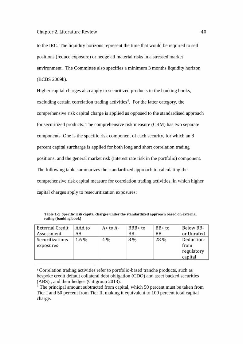
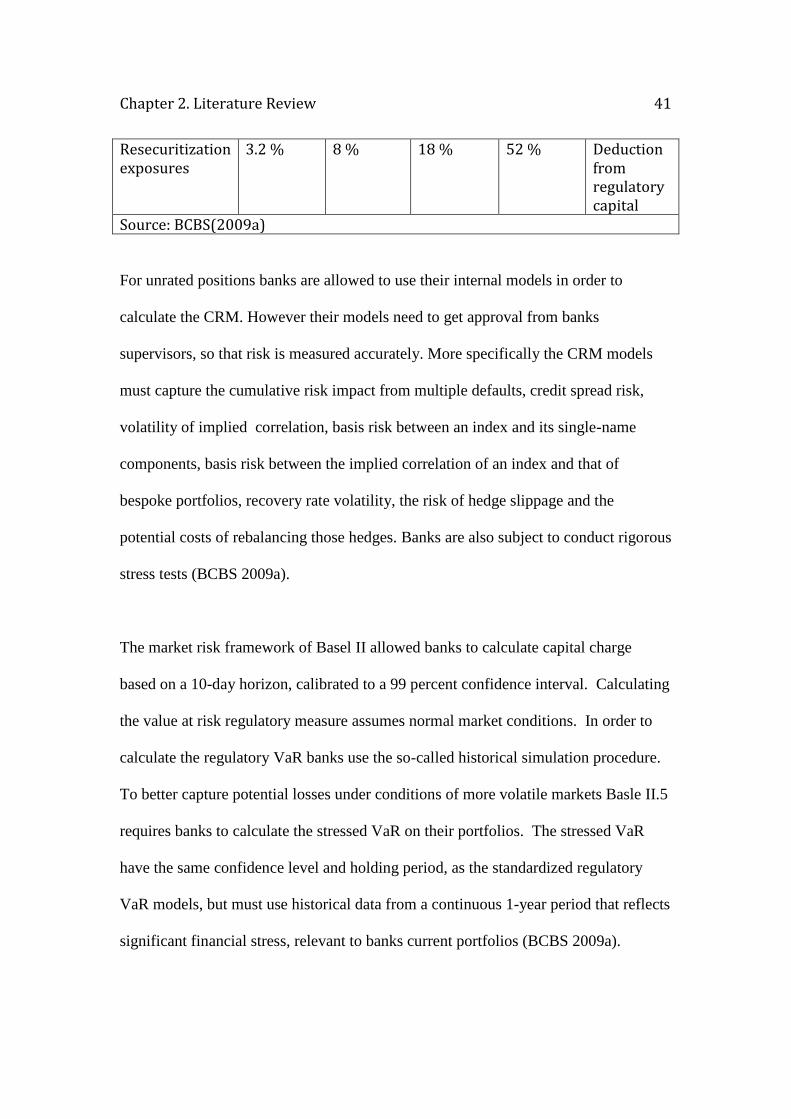
The following table summarizes the standardized approach to calculating the
comprehensive risk capital measure for correlation trading activities, in which higher
capital charges apply to resecuritization exposures:
Table 1-1 Specific risk capital charges under the standardized approach based on external rating (banking book)
External Credit Assessment
AAA to AA-
A+ to A- BBB+ to BB-
BB+ to BB-
Below BB- or Unrated
Securitizations exposures
1.6 % 4 % 8 % 28 % Deduction5 from regulatory capital
4 Correlation trading activities refer to portfolio-based tranche products, such as
bespoke credit default collateral debt obligation (CDO) and asset backed securities
(ABS) , and their hedges (Citigroup 2013). 5 The principal amount subtracted from capital, which 50 percent must be taken from
Tier I and 50 percent from Tier II, making it equivalent to 100 percent total capital
charge.
Chapter 2. Literature Review 41
Resecuritization exposures
3.2 % 8 % 18 % 52 % Deduction from regulatory capital
Source: BCBS(2009a)
For unrated positions banks are allowed to use their internal models in order to
calculate the CRM. However their models need to get approval from banks
supervisors, so that risk is measured accurately. More specifically the CRM models
must capture the cumulative risk impact from multiple defaults, credit spread risk,
volatility of implied correlation, basis risk between an index and its single-name
components, basis risk between the implied correlation of an index and that of
bespoke portfolios, recovery rate volatility, the risk of hedge slippage and the
potential costs of rebalancing those hedges. Banks are also subject to conduct rigorous
stress tests (BCBS 2009a).
The market risk framework of Basel II allowed banks to calculate capital charge
based on a 10-day horizon, calibrated to a 99 percent confidence interval. Calculating
the value at risk regulatory measure assumes normal market conditions. In order to
calculate the regulatory VaR banks use the so-called historical simulation procedure.
To better capture potential losses under conditions of more volatile markets Basle II.5
requires banks to calculate the stressed VaR on their portfolios. The stressed VaR
have the same confidence level and holding period, as the standardized regulatory
VaR models, but must use historical data from a continuous 1-year period that reflects
significant financial stress, relevant to banks current portfolios (BCBS 2009a).
Chapter 2. Literature Review 42
2.1.3 Basel III
Financial regulation, especially the Basel capital requirements have received much
criticism over the latest financial global crisis. One of the most frequent arguments
has been the need to make banks more capitalized as well as having a weak
framework to account for off-balance sheet activities. In December 2009 the BIS
proposed a new set of measures dubbed Basel III. These rules reinforce the view that
the greater the risk to which a bank is exposed, the greater the amount of capital it
needs to hold to protect its soundness and overall economic stability. The new
framework also attempts to deal with procyclicality of capital requirement as well
complementing microprudentail with macroprudential in order to better deal with
credit cycles (D’Hulster 2009).
Under Basel III banks are required to maintain a least 4.5 percent of risk-weighted
assets in common equity Tier I at all times. Tier I capital must be at least 6 percent of
risk-weighted assets. Total capital, that is both Tier I and Tier II, remains the same at
8 percent of total risk-weighted assets. Basel III also tightens the definition of
common equity and additional Tier I and Tier II capital. This Accord places a strong
emphasis on the elements that should be included in the definition of Tier I, which
must mainly consist of common equity and retained earnings.
Chapter 2. Literature Review 43
In addition to the minimum capital requirements Basel III established a new
conservation buffer consisting of common Tier I set at 2.5 percent of the total risk-
weighted assets. The purpose of the conservation buffer aims to protect banks from
potential losses during periods of financial and economic distress. While banks can
draw on the buffer during such periods of stress, the closer their regulatory capital
ratios approach the minimum requirements, the higher the limitations on earnings and
distribution i.e. such banks are expected to lower dividend payments to shareholders,
or share buy- backs until they have improved their balance sheets. The capital
conservation buffer will be implemented in stages by January 2019. Banks are
required to hold a minimum of 0.625 percent of risk-weighted assets starting on
January 2016, and then increase it each year by 0.625 percent rising until 2.5 percent
in January 2019.
With the aim to mitigate procyclicality Basel III has introduced capital
countercyclical capital buffer measures as a complementary to the conservation buffer
capital. The procyclicality of bank capital regulation is related to the interaction
between capital requirements and economic fluctuations. During good times, when
the economy is booming, bank capital should increase, and when the economy enters
into recession bank capital should fall. As evident in the latest crisis, bank excessive
lending in periods of economic expansion, can result in huge amount of losses for
banks when the economy takes a downturn. These losses can weaken the banking
sector, which could amplify economic recessions (BCBS 2010a). The idea of
countercyclical buffer capital measures therefore is for banks to hold higher buffer in
Chapter 2. Literature Review 44
good economic times and decrease during recessions. Taking into account the macro
environment in which banks operate, this measure is a macroprudential tool in
achieving financial stability by means by controlling credit growth in good times and
putting banks in a better financial position to withstand losses during downturns
(Jimenez et al 2012, Getter 2014). The logic behind this measure is that whilst
requiring banks to maintain higher capital ratios in good times increases their capacity
to withstand any unexpected losses, it could also lead to higher lending rates charged
by banks, thereby reducing the demand for credit.
In a forward looking approach accounting for the procyclicality, that the credit cycle
introduces into the real economy, is not a new regulatory tool. Even though it is the
first time that the Basel Committee proposes such measure, Spanish banks have been
subject to countercyclical buffer capital measures since 2000. Despite this measure
being in place, Spain experienced a property bubble, fuelled by excessive credit,
causing severe distress in the banking sector (Getter 2014). Nevertheless, the Basel
Committee introduced countercyclical buffer requirements that would vary between
zero and 2.5 percent of common equity Tier I or other fully loss absorbing capital, to
total risk weighted assets. The size of the buffer will be set by national regulatory
authority, depending on their judgement on credit conditions that could be a hazard to
financial stability.
For the first time the Basel Committee introduced a non-risk based leverage ratio as a
additional measure to risk based capital requirements. The focus on the leverage ratio
Chapter 2. Literature Review 45
derives from the latest global financial crisis in which banks had built up excessive
leverage, which in turn is believed to have exacerbated the crisis (D’Hulster 2009).
The newly introduced standard also acts as a countercyclical instrument. Intuitively
higher capital means lower leverage and vice versa6. This is because in good
economic times when asset prices are rising, bank equity as a proportion of total
assets increases. In contrast, during economic downturns, asset price fall and as bank
capital decreases, leverage is likely to increase. However, it is often argued that
leverage is procyclical with the credit cycle. As evident in the crisis the market
imposed pressure on banks to reduce its leverage, which contributes to falling asset
prices, contributing to greater losses, lower bank capital and decline of credit (BCBS
2010a).
D’Hulster (2009) explains the procyclicality of leverage by highlighting banks’
activities during the credit cycle activities used to manage their leverage, which are
collateralized borrowing, and lending. Under expansionary monetary policy banks
balance sheets grow, and subsequently liquidity supply increases. By contrast when
monetary policy is tight, banks balance sheets shrink, thus the supply of liquidity
decreases. The introduction of a minimum leverage ratio by the Basel Committee,
aims to limit the amount of banks’ debt relative to their equity capital and reinforce
the risk-weighted capital requirements. Currently, the BCBS is testing a minimum
Tier I leverage ratio of 3 percent, and plan to fully implement it by January 2018.
However, the US regulators in 2013 announced the decision to implement a higher
6 The leverage ratio is the ratio of total assets to capital, or Tier I capital.
Chapter 2. Literature Review 46
leverage ratio than that proposed by Basel III. The country’s largest bank holding
companies are required to hold a minimum leverage ratio of 5 percent, whereas their
insured depository institutions subsidiaries must hold a minimum leverage ratio of 6
percent, in order to be considered well-capitalized (Federal Reserve 2014).
Basel III also introduces new liquidity standards in an attempt to avoid a reoccurrence
of a liquidity crisis. The latest financial crisis revealed that despite many banks being
well capitalised, liquidity problems are a major source of financial instability. A
series of papers published by the BCBS, recognizes that capital adequacy regulation is
not enough to prevent a liquidity crisis7 (BCBS 2010b, BCBS 2009a). Therefore, the
Committee proposed a new liquidity framework creating two regulatory liquidity
measures: The Liquidity Coverage Ratio (LCR) and the Net Stable Funding Ratio
(NSFR).
The LCR aims to promote short-term resilience of banks’ liquidity ensuring that it has
enough high quality liquid assets to survive any sudden disruptions in liquidity lasting
30 days. The numerator of the LCR consists of stock of high quality liquid assets,
such as government securities and cash, and the denominator is comprised of cash
outflows minus cash inflows over a 30 day period. Therefore the stock of liquid
assets held should be equal or greater than the net cash outflows.
7 The paper notes that […many banks –despite adequate capital levels-still
experienced difficulties because they did not manage their liquidity in a prudent
manner] BCBS(2010b, pg. 1).
Chapter 2. Literature Review 47
The NSFR aims to promote long-term resilience by encouraging banks to rely upon
stable sources, such as medium and long term funding, to fund their activities. The
NSFR measures the amount of available stable funding (ASF) relative to the amount
required stable funding (RSF). The ratio is intended to measure the minimum amount
of funding that is expected to be stable over a one-year period taking into account the
liquidity characteristics of a bank’s assets as well its off-balance sheet activities. The
amount of ASF is the sum of an institution’s liabilities and capital using available
stable funding assigning different weights (ASF factors) (Getter 2014). In such,
banks capital is assigned 100 percent ASF weight. Consumer deposit liabilities, such
as retail and small and medium enterprises that are considered stable receive a 95
percent ASF factor, whereas those deposits that are considered ‘less stable’ receive a
90 percent ASF weight. Corporate deposit liabilities and public sector lending with
maturities les than one year, as well as other lending with maturities of more than six
months but less than one year, receive a 50 percent ASF weight. Any other liabilities
and net derivatives receivables are assigned 0 percent ASF factor. Thus, higher
weights are given to those stable funding sources that have longer maturities than
those with shorter maturities (Getter 2014). The denominator of the NSFR is
calculated as the sum of the value of assets and funded by the institution assigning
different RSF factors. Assets that are more liquid, in that they can be converted
quickly into cash without any losses, receive lower RSF weights than assets that are
less liquid and require more stable funding receive higher RSF weights. For example
cash assets, don’t require funding hence receive 0 percent RSF weight.
Unencumbered marketable securities with maturities more than a year receive 5

Chapter 2. Literature Review 48
percent RSF weight, whilst unencumbered corporate bonds rated at least AA with
maturity one year or more, would be assigned a 20 percent RSF factor. Gold,
unencumbered equity securities and corporate bonds rate AA- to A-, with one or more
year to maturity, as well loans to non-financial corporations with maturity less than a
year receive a 50 percent RSF factor. Residential mortgages of any maturity and other
unencumbered loans with maturity of one year or more, that receives 35 percent or
less risk weight under Basel II standardized approach for credit risk, would receive 65
percent RSF factor. Loans to retail clients are subject to 85 percent RSF factor and
any other assets receive 100 percent weight (BCBS 2010c). The NSFR must be
greater than 1. So in order to maintain the NSFR equal to or greater than 100 percent
banks could increase their capital when funding longer-term loans with a sequence of
shorter-term loans or diversity the maturity of their own short-term debts (Getter
2014). The NSFR also assigns different RSF weights to various off-balance sheet
activates in order to determine the amount of stable funds an institutions should hold
relative to its off balance sheet exposure that may be need funding over one year
period. The LCR will be introduced in January 2015, whereas the NSFR will be
implemented in January 2018.
To sum up, the ratio of minimum total capital banks will be required to hold by 2019
is set at 13 percent, adding the 2.5 percent conservation buffer and 2.5 percent
countercyclical buffer capital to the 8 percent minimum total capital. These
requirements apply to all globally active banks. However, for larger banks, relative to
the asset size, the so-called globally systemically important banks (G-SIBs) Basel III
Chapter 2. Literature Review 49
has introduced additional loss absorbency or capital requirements. The rationale
behind applying higher capital standard to these banks is based on the impact that
their distress or failure would have on global financial activities. Hence the health of
these banks is perceived to contribute significantly to global financial stability. The
Committee has proposed an assessment methodology in identifying those financial
institutions that would fit in the category of G-SIBs, using an indicator-based
measurement approach.
This approach uses both qualitative and quantitative indicators to determine the
systematic importance of globally significant financial institutions. The identified
G-SIBs would then be grouped into different categories of systemic importance in
accordance to the scores produced by the indicator-based approach, and would be
allocated into different “buckets”, based in their scores of systemic importance,
assigning varying additional capital requirements. These requirements, to be met with
common equity, would range from 0 percent to 2.5 percent of the total risk-weighted
assets (BCBS 2011). For example banks allocated in bucket 1 are required to hold a
minimum of 1 percent additional loss absorbency, banks in bucket 2 should hold 1.5
percent, banks in bucket 3 are required to hold 2 percent and banks in bucket 4 are
required to hold 2.5 percent additional capital. The additional loss absorbency
requirements will be implemented in stages and become fully effective in January
2019. In 2011 the Financial Stability Board (FSB) published the first official list of
identified G-SIBs. The list is expected to be updated yearly by the FSA. The latest
Chapter 2. Literature Review 50
updated official list was published in November 2013, and an additional bank to the
G-SIBs. This brings the total number of identified G-SIBs to 29, (FSB 2013a).
The 27 member jurisdictions and 44 central banks and supervisory authorities agreed
on Basel III proposals for capital and liquidity requirements, together with the
proposed implementation schedules, in September 2010 (Getter 2014). In relation to
US banks, some of the new rules clash with the Dodd-Frank Wall Street Reform and
Consumer Protection Act signed into law in 2010 (the Dodd-Frank Act). The Act is
considered the largest financial regulation overhaul of the US financial sector since
the Great Depression. Amongst other reforms, it addresses capital requirements and
the definition of Tier I capital for the US banking institutions, which differ from what
Basel III and Basel II.5 proposes. For example, the Dodd-Frank Act removes the use
of credit rating agencies. The newly Basel Accords, II.5 and III, both rely on credit
rating agencies to assign risk to various securities, and hence determining the amount
of capital a banks needs to hold. However, given the blame the credit agencies
received in the 2007-09 financial crisis, the Dodd-Frank Act forbids their use. Instead,
the US authorities have had to come up with new standards to determine the risk of
various assets held by banks and apply bank capital requirements accordingly. The
new risk-weighted methodologies implemented by US regulatory authorities take into
account factors such as different loan categories, issuers and the underwriting
requirements of borrowers (Getter 2012). The risk weights would then be multiplied
to all bank assets, and the sum of the risk-weighted assets is then multiplied by a
Chapter 2. Literature Review 51
minimum capital percentage in order to assess how much capital a bank needs to hold
(ibid).
Furthermore, section 171 of the Dodd Frank Act, the Collins Amendment, established
minimum risk-based capital and leverage requirements for all insured depository
institutions, their holding companies and systemically important non-bank financial
companies. The Collins Amendments imposes equal risk capital requirements and
leverage capital requirements to bank holding companies and significant nonbank
financial institutions and insured depository institutions. This is the first ‘floor’ to
which the capital and leverage requirements are subject, established by the Office of
the Comptroller of the Currency, Treasury; Board of Governors of the Federal
Reserve System; and the FDIC (collectively known as the agencies). The second floor
requires the minimum requirements not to be quantitatively lower than the
requirements that were in effect when the Dodd-Frank Act was enacted, in 2010.
The Collin Amendments also eliminates trust preferred securities as an element of
Tier I capital for large bank holdings and systemically important financial institutions.
The exclusion of trust preferred stock from the definition of Tier I capital for insured
depository institutions became effective at the time of the enactment of Dodd-Frank
Act, whereas the Collin Amendment places this requirement to bank holding
companies with consolidated assets of $15 billion or more. The phase time given to
US banks to adjust to these requirements is three years, beginning on January 1, 2013.
Chapter 2. Literature Review 52
Under Basel III trust preferred stock are no longer eligible for Tier I capital treatment.
However, the phase in period under Basel III is 10 years, beginning on January 1,
2013, unlike the shorter phase in schedule outlined under the Collin Amendment.
Despite the difference between the requirements set by the Dodd-Frank Act in US and
the Basel III requirements, these regulatory measures attempt to impose higher capital
requirements in an attempt to promote a safer and sound financial system.
2.2 Related Literature
The literature on capital adequacy requirements falls naturally into three parts. In the
first place there are the proponents of capital adequacy adducing various arguments as
to how capital adequacy may reduce risk in banking. In a second, much
smaller, category are those banking experts who argue that capital adequacy is not
effective in decreasing banking risk, and may even increase it. Finally, there is the
very small number of studies that have examined this question empirically. In the first
category are various studies coming principally from the Bank for International
Settlements (BIS).
While the literature on capital adequacy is vast, until recently very little empirical
evidence was available on the relationship of probability of banks default and capital
adequacy. As surprising as this seems, the lack of literature on this topic is also
confirmed in Barrell et.al. (2009) in which the authors attempt to estimate the benefits
of capital adequacy in reducing banking crises. Furthermore, King et al (2005) states
Chapter 2. Literature Review 53
that even though since the 1990s the banking system has undergone fundamental
changes, research into the causes of distress has significantly slowed.
A large body of literature examines the role of capital requirements on risk taking.
One of the arguments for imposing capital regulations is that it will provide banks
with the incentives to take less risk. Repullo (2002) suggests that higher capital ratios
mean that banks shareholders would incur higher capital losses in the event of default,
and thus they reduce banks incentives for risk taking. His analysis makes use of a
dynamic model of imperfect competition in which banks are assumed to have two
investment strategies; invest in prudent assets or gambling assets. He argues that
capital regulation ensures the existence of a prudent equilibrium, because capital
requirements do not affect banks’ charter value and restrains gambling investment by
imposing higher equity losses to the bank shareholders in the event of default
(Repullo 2002).
Furlong and Keeley (1989) and Keeley and Furlong (1990) also examine the impact
of capital requirement from a risk incentive perspective. They employ a state-
preference model in which the option value of deposit insurance is taken into
consideration. This approach was first used by Merton (1977), in a study in which
he derived a formula used in the option pricing model, showing that deposit insurance
can be viewed as a put option of the value on bank assets with an exercise price equal
to the face value at maturity of banks debt i.e. bank deposits (Santos 2000). Merton’s
study also concerned the impact of deposit insurance and risk-taking incentives, and
Chapter 2. Literature Review 54
suggests that regulators need to supervise both the risk of assets and leverage of
insured value-maximising banks (Keeley and Furlong 1989). The importance of the
studies conducted over the effect of deposit insurance and risk-taking can be thought
of as the logic behind the decision of regulators to impose capital requirements. As
Keeley and Furlong (1989) state ‘ Concern over the risk exposure of the federal
deposit insurance system has been a major factor behind the increase in capital
standards in banking in the 1980s’ (Keeley and Furlong 1989, pp. 883). In response
to the risk-incentives behaviour that deposit insurance brought about in banks, studies
such as Merton (1977) called in the need for bank regulation, as explained above.
This led to many studies focusing on the effect of capital requirements on bank risk-
taking.
The theoretical and empirical evidence on whether increasing capital ratios lower risk
taking is not conclusive. For example, the studies of Koehn and Santomero (1980),
Kahane (1977), Kim and Santomero (1988) using a mean-variance model, argue
that higher capital ratios could in fact increase the risk of utility maximising banks.
However, Keeley and Furlong (1989) argue that once the option value of deposit
insurance is taken into consideration, higher capital standards lowers bank risk
incentives. They argue that this is because, the value of marginal value of deposit
insurance option in relation to increasing asset risk declines as leverage declines.
Therefore, restricting the leverage on banks should decrease risk incentives.
Sheldon (1996), also used the Black-Scholes formula to examine the risk effect of
capital adequacy regulation for several G-10 countries. He examines 219 banks from
Chapter 2. Literature Review 55
a variety of countries over the period 1987 to 1994 to study the risk effect of the Basel
I Accord. With reference to the US his findings suggest that bank asset volatility
increased as banks raised their capital ratios. The positive relationship between asset
risk and capital ratios was found in banks for the period 1990-1992, reflecting the
Basel Accord regulatory implementation. However, examining the period before the
implementation of the capital requirements Sheldon’s findings are similar to the post-
regulation period. That is to say that bank asset volatility increased for both bank
groups, those that raised capital ratios as subject to Basel regulation and those that
didn’t prior to the capital regulation being in place. However, in Japan he finds that
the asset volatility and default probability of Japanese banks over the sample period
fell, even though most banks increased their capital ratios.
Montgomery (2005) also studies the risk incentive behaviour of Japanese banks for
the period between 1982-1999. The analysis looks at how the impact of risk-based
capital ratios affect portfolio risk adjustment for both domestic and international
banks. Similarly, to Sheldon (1996), the effects of capital requirements on banks
portfolio decision is conducted by examining banks’ risk incentives,- as measured by
the sensitivity of four different assets such as total assets, loans, corporate bonds and
governments bonds- prior to the Basel requirements and post- Basel requirements.
The study concludes that the low capitalized international banks in the period post-
Basel requirements greatly shifted towards holding less risky assets. More specifically
these banks shifted their asset portfolio from the risk-weighted assets such as loans
and corporate bonds to riskless assets such as government bonds. This behaviour is
Chapter 2. Literature Review 56
found only in the post-Basel period. In terms of the domestic banks this effect is not
found, so that the Basel capital requirements did not affect their asset portfolio.
In contrast to these views Blum (1999) argues that capital requirements increase bank
risk taking. He employs a discrete time model to study the intertemporal effect that
the capital adequacy rules have on the behaviour of banks. He argues that one of the
effects of the capital requirements is a reduction in the expected profits, which
reduces bank losses if it defaults. He argues that under binding capital requirements
raising equity is excessively costly, and in a dynamic model the value of equity for a
bank is more valuable tomorrow than today. In what follows, the only option left for
banks to increase the amount of equity tomorrow would be to increase risk today.
This way he argues the effect of capital requirements is opposite to what is perceived.
Similarly, Gale (2010) argues that higher capital requirements will not necessary
reduce the level of risk taking in the banking industry. This conclusion is reached
when the impact of capital requirements is analysed within a general equilibrium
framework. He argues that in a banking environment, which he calls it a ‘casino
banking’, that is driven by target return on equity, rising capital requirements induce
bank managers to take on additional risk to achieve their desired rate of return.
Other studies, such as the one of Alfon et al (2004), are concerned with the impact
that capital requirements has on the amount of capital a bank decides to hold. The
analysis looks at UK banks over the period of 1998-2003, and states that banks do
hold buffer capital in addition to what is required. The authors identify risk
Chapter 2. Literature Review 57
management, market discipline and the regulatory environment as the main factors
that influence the amount of capital held by banks. However, the regulatory
requirements are the largest determinant affecting capital adequacy as opposed to the
other considerations. These findings are similar to Ediz et al (1998) which study
looks at the impact of capital requirements on the internal decisions of banks capital.
The empirical evidence there suggests that the requirements strongly affect the
amount of capital a bank would like to hold. In addition the paper states that banks
adjust their capital ratios through the issue of equity rather than adjustment in balance
sheet compositions. These results, suggest that capital regulation can significantly
influence bank decision making on equity issue rather than risk management.
Some argue that the introduction of capital requirements was to blame for bringing on
a credit crunch in countries like the US and Japan. Furfine(2000), examines the
impact of changes to capital requirements on US banks. The analyses examine the
role the Basel Accord played on the credit crunch the US experienced in the 1990s.
Banks responded to the risk based capital regulation by shifting their portfolios into
government securities. Banks reduced their commercial and industrial lending, and
increased their investment in government securities. This precipitated the credit
crunch (Furfine 2000). During the same period the US also experienced a recession,
suggesting that the decreased credit supply was the cause of the negative shock in the
economy. However, a graphical representation of banks portfolio changes shows that
the decreased supply was evident well before the start of the recession and well after
the following US expansion had begun. Supporting these findings, the author also
Chapter 2. Literature Review 58
points to the previous recession that the US had experienced and states that the shift in
bank portfolios was the reverse of that in the recession of the 1990’s. In previous,
economic contractions, commercial lending rose and investment in government
securities either fell or remained fairly unchanged. Taking into account the marginal
costs banks incur as a result of regulation, the study examined the impact of
implementing capital requirements on lending growth and capital ratios over the
period of 1989-1997. The estimated results show that capital requirements played a
role in explaining the decline in loan growth and the rise in capital ratios in the US.
Similarly, many researchers have attributed to the credit crunch in the Japanese
banking system to the introduction of capital adequacy regulations. Montgomery
(2001) takes the analysis further by investigating the relationship between risk-based
capital ratios and lending, and how the credit supply might have had had an impact in
the real economy. Therefore, the research is based on both at macro and micro level.
Calculating the capital adequacy ratios from individual banks and using an
instrumental variable estimation method the author provides evidence on the micro
level of Japanese banks over the period of 1982-1999. The study takes into account
the different requirements standards between international banks, which under the
Basel Accord are subject to an 8 percent capital ratio requirements, and domestic
banks which are required to maintain a 4 percent MOF(Ministry Of Finance) ratio
requirement. There is some sort of agreement, in the Japanese banking system
literature, that the new standards limited bank activity at an international level. A
number of banks were forced to close their international branches so that they were
Chapter 2. Literature Review 59
under the MOF regulation framework. The analysis shows that stricter capital
adequacy requirements greatly reduced bank lending in Japan in the early 1990’s
most significantly in the case of international banks. Evidence suggests that domestic
banks that were under less strict capital requirements, responded rather less to the
increased requirements in terms of credit supply. The macroeconomic analyses,
suggest that the reduction in credit supply contributed negatively to the real economy
resulting in the ‘lost decade’ the Japan has experienced.
Martin’s (1977) econometric study testing for the determinants of banks failure is one
of few that used a measure of capital to risk-weighted assets. The Basel 1 ratio
requirement did not take effect until 1993, making it too early for it to be tested in his
study. But even the ratio of capital to assets, unweighted for risk, appears significant:
as capital adequacy rises, the probability of failure declines. He constructs an early
warning signal model estimating the probability of future bank failure as a function of
variables taken from the current period’s balance sheet and income statement during a
seven- year period during the 1970s.
The approach, as termed by him- ex post empirical- in which a sample of failed banks
were compared with those banks that did not fail. The dependent variable, a dummy
variable, is the occurrence of bank failure. The independent variables are drawn from
a set of 25 financial ratios which he classified them into four groups; (1) asset risk (2)
liquidity; (3) capital adequacy; and (4) earnings. In what became a standard approach
he ran several different specifications in which variables are dropped or added to the
model one at a time based on their individual significance and their contribution to the
Chapter 2. Literature Review 60
overall fit of the model. He finds that capital ratios- gross capital/risk asset ratio-
liquidity measures and profitability were the most significant determinants of failure
during that period. However, he states that the level of significance differs among
periods. The overall quality of the equations was “best” in the later periods i.e. in
1974 reflecting the development of the banking system after 1970. Because in the
earlier period bank failure was infrequent, and the overall loan losses suggested that
earnings and capital adequacy levels played a minor importance to the bank’s ability
to survive. Bank failures were often associated with fraud and local economic trends
which are difficult to obtain by examining bank financial statements whereas the
recession-related asset problems are well reflected and were important in the later
years. In reference to the level of loan losses, prior to 1973, such losses were at a
minimum. However they greatly increased after that and badly affected the entire
banking system. Therefore, he emphasised that the soundness criteria of banks varies
over the business cycle. He concludes by stating that these findings are at variance
with the literature on bank failure during the 1930s, which suggests that capital
adequacy is little or not related to banks failure even under conditions of significant
stress in the banking sector.
The Basel Committee on Bank Supervision, along with the staff at the BIS engage in
the research and study of international banking. In August 2010 they published a
paper which assesses the long-term economic and costs of strengthening capital and
liquidity requirements, in terms of their impact on output. The analysis is based on
the assumption that banks have completed their transition phase to the new levels of
Chapter 2. Literature Review 61
capital and liquidity. Reducing the frequency of the banking crises has substantial
benefits. The analysis reports that a 1 percent point reduction in the probability of
crises will gain around 0.2 percent of GDP per year, whereas when crises have long-
lasting effect, it will generate a benefit between 0.6 percent and 1.6 percent of GDP
per year. It is estimated that increasing capital ratios from 7 percent to 8 percent, with
no change in liquid assets, reduces the probability of banking crises by one third ( e.g.
from 4.6 percent to 3.0 percent). The overall message conveyed is that benefits
exceed the costs in the long run and ‘there is considerable room to tighten capital and
liquidity requirements while still yielding positive benefits, measured in terms of
output’ (BCBS, 2010d, pg. 28)
Around the same period, the Macroeconomic Assessments Group (MAG) at the BIS
presented a paper concerned with the need to phase in the new regulation in a manner
that relates well to the ongoing economic recovery. Higher capital standards affect
the economy as banks increase their capital levels by increasing the cost of borrowing
and reducing the supply of new loans. The MAG group used a two-step approach, in
which the first step is to estimate the effect of higher capital standards on lending
spreads and lending volumes using both statistical and accounting-based analyses.
These estimates then, serve as inputs to the macroeconomic forecasting models which
are used to assess the effect of changes to lending spreads and volumes on
macroeconomic variables. Banks behaviour when faced with tighter capital and
liquidity standards depends also on the length of the period during which the
Chapter 2. Literature Review 62
requirements are phased in. When banks are allowed time to adjust to new
requirements, they may respond differently, in that they have additional time to
employ different strategies of capital raising such as retaining earnings, issuing
equity, shifting liability composition, hence mitigating any adverse effect on
aggregate activity. Also the estimated impact transmitted from increased capital
ratio could be offset by other benefits associated with the new requirements. Because
banks become more robust, they face lower debt funding cost and required ROE
target. This in turn should reduce the need to either raise lending rates or limit the
quantity of new loans. Also other available sources of finance such as capital markets
and retained earnings for non-financial corporations are likely to lessen the impact of
changes in credit growth on economic activity (MAG 2010).
Barrell et al (2009) employs a multivariate logit model to relate the probability of
bank default to a vector of explanatory variables. Their approach consists of pooled
data on a number of crises from 14 OECD countries and focuses on capital adequacy
as an indicator of banking crises. The authors then trace the impact of banking crises
on the economy focusing on the user cost of capital. The dependent variable is
defined in terms of observable stresses to a country’s banking system. Using a general
to specific approach, the crisis prediction model reveals that unweighted capital
adequacy and the liquidity ratio alongside real house price growth are the most
important determinants of the probability of financial crises in the OECD countries.
Using data for the period of 1970-2007, they predict that, given the levels of capital
and liquidity in 2006, the probability of crises could have been reduced by more than
Chapter 2. Literature Review 63
6 percentage points, if the level of capital and liquidity were increased by one
percentage point (Barrell et al. 2009).
King(2010), from the monetary and economic department of the BIS, examines the
loan pricing implication of higher capital requirements. While banks adjust to new
requirements in various ways this paper is concerned with the possibility that banks
seek to pass on the additional costs by raising the interest rates on loans to their
borrowers. Calculating a representative bank’s balance sheet and income statement
using data for 6,844 banks from 13 OECD countries between 1993 - 2007, the study
maps how changes in a bank’s capital structure, the composition of its assets and the
measurement of risk-weighted assets(RWA), affect the different components of net
income using accounting relationships. Measuring changes of a representative bank’s
net income and shareholders’ equity associated with the new regulation standards,
allows the author to calculate any increase in lending spreads required to realize a
given return on equity (ROE). Bank lending spread here is defined as ‘the spread
between a bank’s cost of liabilities and the average rate charged on its loan portfolio’.
The assumption here is that banks price their loans in such manner that they cover the
marginal cost associated with loan production. Also, assuming no change to other
variables such as bank’s ROE or cost of debt, a 1 percentage point increase in the
capital ratio can be offset by increasing the lending spreads by 15 basis points.
Whether banks will be able to pass on these additional costs to consumers, King
argues, amongst others, depends on the elasticity of the demand for loans. However,
if the ROE and cost of debt is allowed to decline by 10 basis points for each 1
Chapter 2. Literature Review 64
percentage point increase in capital ratios, the increase in lending spreads is reduced
to 13 basis points.
King (2010) also points to the work of Elliot (2010) which by applying the same
accounting principles using data for the US banking system he examines the changes
of interest rates charged on loans when banks are faced with tighter capital
requirements. He assumes that the representative bank holds only loans, which are
funded by equity, deposits and wholesale funding. Banks will charge an interest rates
which ensures they receive their desired target ROE after taking care of other costs
such as the cost of liabilities and other fixed costs. Elliot estimates that if the ratio of
common equity required for a given loan is raised by 2 percent, assuming no other
adjustments, then banks will increase lending spreads by 39 basis point in order to
meet their target ROE of 15 percent. However he argues, that if banks were to reduce
their ROE to 14.5 percent this would make the required increase to fall to 9 basis
point together the cost of liabilities to decrease by 10 basis points. His proposition of
a decline(not shown empirically) in ROE and the cost of liabilities are based on a
modified Modigliani-Miller framework, which is based on the assumptions that the
weighted average cost of capital (WACC) does not change for different capital
structure choice. He concludes that banks could adjust to the new requirements by
choosing a combination of actions that would mitigate the effects on pricing or
availability of bank loans.
Chapter 2. Literature Review 65
But these are studies of the impact of capital requirements in lending spreads and
ROE, rather than on the likelihood of default, which the capital requirements are
supposed to affect.
Toporowski provides a theoretical argument, in which he states that rising capital
adequacy requirements under conditions of inelastic equity capital supply, has the
effect of forcing non-financial firms into debt. Requiring banks to increase their
capital reduces the amount of capital available to non-financial firms. When banks are
faced with tighter capital regulation they have to adjust their capital accordingly.
There are various ways in which banks adjust their required capital ratios. Either one
of them will have a negative impact in the capital market. The higher the amount of
capital held by banks, the lower the quantity available to nonfinancial firms seeking
capital finance. Such firms are left with no option other than to raise their needed
capital through the issue of debt instruments. Hence, firms are forced to borrow more
than planned, which in turn reduces future fixed capital investment. Toporowski
argues that ‘enforced indebtedness’ increases the financial fragility of the economy.
Firms instead of reducing the amount of debt held, now have debt in excess of what
they planned which can be accommodated in two ways. Firstly, companies can hold
larger amounts of liquid assets. But this is not efficient since it means that the capital
that firms have issued is being ‘wasted’ by being held as financial asset rather than
being used to expand production or fixed capital. Alternatively, firms could reduce
their future fixed capital investment in order to be able to have those liquid assets.
Therefore, the excess debt level being held by firm as a consequence of higher banks’
Chapter 2. Literature Review 66
capital regulation requirement reduces productive investment below what it would
otherwise be. The reduced productive investment then also reduces the cash flow of
firms and their ability to service their debt. Therefore, higher capital requirement that
aims to circumvent banks unsoundness, encourage firms to reduce their productive
investment in fixed capital in response to their increased indebtedness. Toporowski,
notes that such reduction in is the key determinant in causing the real economy to
enter in recession. Furthermore, as history reveals the case of 1930s or Japan after
1992, excess debt can turn recession into economic stagnation and depression
(Toporowski 2008, 2009).
A theoretical contribution on the topic is provided by Martinez-Miera (2009), in
which he argues that higher capital standards reduce both banks leverage and, for
given asset risk, the probability of bank default. The analysis assumes that
entrepreneurs respond differently to changes in loan rates in the presence of moral
hazard between banks and entrepreneurs. As a starting point, the paper emphasizes
the benefits of having higher capital requirements, the capital buffer effect. When
loan defaults are imperfectly correlated, the higher the capital requirements are, the
higher is the ability of banks to absorb any losses that derive from non-performing
loans, without undergoing failure. On the other hand, when the correlation is high a
bank is unable to meet the demand of its depositors hence no buffer exists and the
bank defaults. As banks face higher capital requirements, they tend to charge higher
loan rates to compensate the higher cost of capital imposed by higher regulatory
standards. This is the risk-shifting effect, as entrepreneurs now face higher costs and
Chapter 2. Literature Review 67
they shift their investment into riskier projects in a bid to have higher returns. As a
consequence they are more prone to default on their loans and the bank is more likely
to default as a higher fraction of its loans will default. A different point of view is
given to the margin effect as capital requirements are increased. Assuming that loan
rates are increased the bank earns higher rents on the non-defaulting loans. This
provides the buffer capital that serves as a cushion to absorb losses. However if all
projects default at the same time, that is when loan defaults are perfectly correlated,
the probability of banks failure increases. By contrast, when the correlation is low, the
effect of higher capital requirements is negative, that is the probability of default
decreases. The overall conclusion of the paper is ambiguous. The author also
provides a numerical solution, which shows that the relationship between capital
requirements and the probability of banks default is non-monotonic (Martinez-Miera
2009).
A weakness in the current literature is the definition of capital adequacy. Although it
is supposed to be an approximate for the Basel definition of Tier one capital,
researchers have adopted different measurements of capital ratios in their analyses as
an approximate for the Basel Accord capital requirement ratio. Barrell et al (2009),
uses the unweighted capital- capital to loan ratio measures- in their analysis.
Montgomery(2001), uses the book value of each banks’ net worth as reported in the
annual ‘yukashoken hokokusho’8 as a proxy for Tier 1 capital ratio. Capital adequacy
is measured by various forms of the basic capital/asset ratio, with our without debt
8 Annual Securities Report
Chapter 2. Literature Review 68
capital in the numerator in Martin’s (1977) study. The BIS studies refer to the broad
definition such as Tier one or total capital as the target ratio of tangible of tangible
common equity to risk weighted assets, including voluntary capital buffer and not the
required minimum level set by regulators.
Estrella et al (2000), state that a good measure of capital adequacy should be strongly
linked with bank failure. The study compares the effectiveness of different types of
capital ratios in forecasting bank failure. As explained above, the calculations of
bank’s capital adequacy ratios are somewhat complex and guided by a formula that
complies within the Basel standards framework. In contrast Estrella et al (2000)
makes use of other accounting-based ratios, arguing that some of these ‘….ratios
contain valuable information and virtually costless information, and therefore have a
role in an overall framework for regulatory capital’ (pg 34). The empirical results
show that that simple ratios, such as the leverage ratio and the ratio of capital to gross
revenue, perform just as well as risk-weighted ratio in predicting predict bank failure
over one or two year time horizon. However, the risk-weighted capital ratio
predicting ability, defined as the ratio of tier 1 capital to risk-weighted assets,
improves beyond the one-or two-year horizon.
The above literature review suggests that bank risk is determined by the composition
of a banks’ balance sheet. By evaluating banks balance sheet and most importantly
by measuring the weighted risk assets and setting up capital adequacy ratios in
proportion to the riskiness of those assets, bank managers and regulators can reduce
the level of riskiness, hence lower the probability of banks default or insolvency.
Chapter 2. Literature Review 69
However, as its discussed below, the case of banking in Japan over the last two
decades suggests that bank risk may be linked to developments in the economy at
large in ways other than bank-risk taking impacting on the ‘macroeconomy’ in which
banks operates. The banking crises of Japan show that risks may be in banks’ balance
sheet but the original source of bank risk comes from macroeconomic shocks. These
facts reflect the credit cycle literature inspired by Keynes 1913, that a stable economy
is a necessary condition for low risk and adequate bank capital. In “How Far are
Bankers Responsible for the Alternations of Crisis and Depression” written in 1913,
Keynes puts forward a simple model illustrating how banks can induce fluctuations in
the economy. The fluctuations are as a result of over-investment during economic
booms and under-investment during recessions (Toporowski 2005). The simple idea
is that banks hold ‘free resources’ which represent savings ‘of the community’ which
are held in current account deposits with banks. And it is these deposits that banks
lend out for business investment. However, savings are also held in the form of other
financial assets held by the public. When business investment has reached high
levels, and most importantly when some of the investments undertaken by firms are
not as profitable, banks realize that they need to arrange more credit to support
investment projects. Recall that savings of the community represents current accounts
held with banks and the purchases of financial asset by the public. And when banks
try to arrange finance by means of selling financial assets, to the public, the
community’s savings will not be sufficient to sustain over-investment. Keynes states
that it is then that banks realize that what they considered to be liquid assets have now
become illiquid. He then argues that this is bound to lower the quality of assets banks
Chapter 2. Literature Review 70
hold (Kregel 1992). Naturally then banks respond to this by reducing lending and
increasing interest rates. It is this process, Keynes argues, that causes banking
difficulty and subsequently a crisis.
Taking macroeconomic conditions into perspective in the regulatory framework has
been a growing concern of many observers in the wake of the latest financial crisis. A
common consensus from a wide range of researchers is that the regulatory framework
needs to shift away from the microprudential approach to macroprudential regulation
(Kashyap et al 2010). However, Crockett 2000; Kashyap and Stein 2004, Borio 2003
and others have highlighted the need to focus more on a macroprudential regulation
before the crisis erupted. More recently, Kashyap at al 2010, Borio 2011, and Tarullo
2014, have contributed to the literature in favour of macroprudential regulation. A
microprudential approach is largely focused in preventing the failure of banks at the
individual level. In contrast macroprudential regulation concerns the financial system
as a whole. Kashyap et al (2010) state that microprudential regulation is based on
partial-equilibrium conception whereas macroprudential ‘ recognizes the
importance of general-equilibrium effects, and seeks to safeguard the financial system
as a whole’ (pg 1).
Tarrulo (2014) argues that macroprudential needs to be combined with the current
capital and liquidity requirements, which are largely based on microeconomic
foundations. He suggests four main propositions that should be incorporated in the
regulatory framework for large financial institutions. He proposes that
Chapter 2. Literature Review 71
macroprudential regulations should dominate in the regulatory and supervisory
framework for these firms. This is because large financial institutions are prone to
common stresses because of their interconnections with each other and thus they
cannot be considered in isolation from the rest of the financial system. The second
proposition concerns resiliency, which should be the central in the macroprudential
regulation. He claims that macroprudential capital requirements are just as important
as the microprudential approach which requires individual banks to hold capital in
able to increase its ability to withstand any losses. He refers to the stress test
conducted over 19 largest bank holding companies as an important starting point
towards macroprudential orientation. Stress tests can be used as a forward-looking
assessment of future potential looses under stipulated adverse economic conditions.
For example he suggests that these test should incorporate particular risk factors to the
financial system, such as house prices, as well as adverse economic conditions, such
unemployment. This approach is bound to lower the level of distress and the
probability of failure for large financial institutions. The stress test was conducted in
February 2010 on banks with assets worth more than $100 billion. The test aimed to
evaluate the financial position of these banks, to ensure that they had adequate capital
buffer to withstand any losses and to maintain lending even under more severe
economic conditions. Each bank’s capital was assessed using a two-year ahead
hypothetical adverse scenario. The degree of stress for each bank was determined by
assuming possible losses accruing on risky loans, assets and trades in the next two
years. The level of stress was then used to determine the capital buffer position for
each bank, i.e. whether a particular bank needs to increase the capital level or not.
Chapter 2. Literature Review 72
As a third proposition, Farullo argues that time-varying measures will play a limited
role at a macroprudential perspective. In the arguments of countercyclical regulatory
tools, such as attempting to restrain any rapid credit extensions or asset prices and
relax those restraints under weak economic conditions, he highlights some of the
difficulties regulators might face in order for these tools to be effective at the
international level. Some of the issues concern the question of having the right
measure of excess or systematic risks, a suitable agency in taking macroprudential
decisions, the speed of these measures to take effect after their implementation, and
the right calibration of measures which would target any excesses without affecting
the availability of credit in the economy.
The last point made by Farullo is related to the structural vulnerability that results
from short-term wholesale funding. He states that large firms that substantially rely on
short-term wholesale funding should be subject to higher capital and liquidity ratios.
Kashyap et al (2010) also advocate macroprudential regulation. Their study discusses
the potential problems associated with the microprudential approach that could lead to
more unnecessary problems that would harm the economy. For example, when a bank
choses to adjust its regulatory capital ratios by means of changing the composition of
Chapter 2. Literature Review 73
the assets in the denominator9, thereby shrinking the assets this could have
implications for the economy if a large fraction of banks are in the same position.
Therefore when banks simultaneously attempt to raise their capital ratios by reducing
lending this is bound to harm the economy. To overcome the social costs related to
excessive balance-sheet shrinkage they propose a set of macroprudential tools.
Among others, time-varying capital requirements are proposed as a macroprudental
tool in response to the balance-sheet shrinkage. They suggest that banks should be
required to hold higher capital ratios in good time than in bad times. This way, in the
event of unexpected or unpredicted shock banks could rely on their buffer capital
without having to shrink their balance sheets significantly. They refer to a study
conducted by Kashyap and Stein (2004), which show that time-varying capital
requirements are the optimal scheme in a model where the objective of a social
planner is to both protect the deposit insurance funds and maintain credit creations
during economic downturns. A further point in Kashyap et al. (2010) is that in bad
times, the market may play a more important role that capital requirements. That is
because, when banks have a large proportion of risky assets in their balance sheet, and
hence a shortage of capital, it is highly likely that the market would provide funds to
these banks. Therefore, the capital regulatory ratios in good times must be
significantly higher than the market-imposed standard in times when risks are
believed to be more prevalent.
9 Regulatory bodies are not concerned how an individual bank achieves its capital
requirements standards, i.e. a bank could meet the capital regulatory standards by
changes in the numerator or denominator.
Chapter 2. Literature Review 74
Capie and Wood (2013), suggest that bank regulation is not necessary if governments
do not underwrite banks. Based on the evidence that the UK banking history reveals
they argue that banks should be left to choose their own capital ratios. They indicate
that at the end of the 19th century capital ratios of UK banks averaged at around 10-12
percent amongst all banks, declining from the 15 percent level held in the mid 1870s.
In the First World War period UK banks capital ratios fell to around 7 percent. This is
argued to have been due to the high volume of government bonds banks held in their
portfolios and therefore they adjusted their capital ratios in accordance to the riskiness
of their assets. This was also evident during the Second World War period. As banks
increased their holdings of gilts and their capital ratios fell to around 3 percent. The
authors argue that if these capital ratios were to be converted in the requirements of
the Basel Accord they would be subsequently higher so that they would reflect the
quality of the assets banks held at the time. For example they argue that during the
1920, that is immediately after the First World War, risk-weighted assets as reflected
the Basel rules, would indicate capital ratios of the order of 14 percent. The capital
ratios of banks during the 1960s, which were around 4-5 percent, according to the
Basel requirements should have been around 13 percent. The authors then argue
against the current regulatory framework set by the Basel capital requirements as well
as the Volker rule which separates investment banking activities from retail banking.
The rationale behind this argument rests upon the evidence provided by the history of
the British banking. In addition they argue that these rules that emphasise the
importance of banks to avoid failure could be misleading. This is because banks
should be left to fail in an orderly fashion. Once banks face the possibility of failure
Chapter 2. Literature Review 75
they would take responsibility for their actions, and thus they would be the best
judges in deciding their needed capital ratios. In such a system banks would have to
be sensible in choosing capital ratios to reflect the riskiness of their assets since
failure in doing so would compromise their survival in the banking business.
Kuritzkes and Scott (2009) argue that capital regulation is not sufficient to prevent
bank failures, and it needs to be complemented with more effective market discipline.
They argue that the insufficiency of the minimum capital regulation to prevent bank
failure was reflected in the high capital ratios banks held prior to the 2007-08 crisis.
The evidence suggests that prior to the crisis of 2007-08 the top 20 US banks had
capital ratios around 11.7 percent, well above of the minimum capital requirements.
However, this was followed by the largest bank failures since the Great Depression.
The article argues that when capital requirements and banks risk-taking are
imperfectly correlated, the regulatory capital constraints could lead banks to seek
higher returns on the additional capital. Also, higher capital requirements could push
banks into the unregulated banking sector, a phenomenon that became evident in the
crisis. They argue that market expectations would play a more important role than the
Basel capital requirements.
Admati and Hellwig’s latest book, ‘The Bankers’ New Clothes’, argues that the best
way to achieve a safer and healthier financial system is to require banks to hold much
higher equity levels. The proposed equity levels are at least between 20-30 percent of
their total assets. They argue that rising equity levels would not reduce lending as

Chapter 2. Literature Review 76
perceived by many. This is because listed banks can raise money by issuing new
shares, and if the funds raised are used to make loans then higher equity levels would
increase lending rather than curb it. For banks not listed on the stock exchange, the
alternative option is to reinvest their earnings. Even though there would be a
transition problem for this category of banks, after some time their lending would be
the same as before.
The distinct feature of this proposition is that it its a clear departure from the Basel
capital requirements. The later, with reference to Basel III capital requirements,
require banks to hold at least 7 percent of their risk-weighted assets, whereas Admati
and Hellwig proposed equity levels related to banks’ total assets. They criticise the
Basel approach and argue that this in turn has substantially reduced banks’ equity to
total assets. The main message of this book is that reducing banks reliance on
borrowing, banks could become healthier by reinvesting their profits and raising
equity in the capital markets, like any other company does. This would lead to a safer
and healthier banking sector ‘..better able to support the economy’ (Admati and
Hellwig 2013, pg. xi). However, to claim that higher equity levels, achieved by
issuing new shares do not impose any costs to the society could be misleading. As
argued, one of the implications of forcing banks to hold higher capital ratios by the
issue of new capital is the crowding out of capital issues by non-financial
corporations. This would then reduce their productive investment, damaging the
economy. This is the core message of the capital market inflation theory of
Toporowski.

Chapter 2. Literature Review 77
The other misleading message that the Admati and Hellwig analysis conveys is the
claim that when banks hold more equity then shareholders will bear the risks rather
than creditors and taxpayers, and thus ruling out any imposed-cost to the society as a
result of increasing equity levels. Banks’ shareholders are mainly pension funds,
insurance companies and intermediaries holding society’s long-term savings. Thus,
to claim that when shareholder are left bearing the risks of the activities undertaken
by banks, then no losses are transmitted to ordinary people is misleading since banks’
shareholders are ordinary people of the society.
This argument is highlighted also by Coppola (2013), which contributes to the capital
requirements literature by showing that there is no difference between equity and
debt. She claims that both equity and debt are claims on a bank’s assets, when it fails,
or its income, when it is a going concern. When a bank fails the only real difference
between a depositor, a bondholder and a shareholder is the seniority of their claims.
She build a hypothetical scenario showing that if for example a bank’s Tier I capital
ratio, which comprises shareholders fund and retained earnings, is 3 percent, and if a
bank suffers losses and it has to write down 3 percent of its assets then the
shareholders funds are wiped out. If losses increase, junior bondholders are next in
line. Once a bank declares that it is in financial distress or failed, junior bondholders
are liable to have their bonds converted to equity, hence becoming ordinary
shareholders. When and if the bank recovers then they can enjoy dividend payments.
However, there is the possibility that their funds would be wiped out, as happened in
Chapter 2. Literature Review 78
the case of the Dutch bank SNS Reaal. As it turned out their investment was saved
when the Dutch government took over their claims when rescuing the bank.
Nevertheless, the point here is that if the government would have not rescued the
bank, junior bondholders together with shareholders funds would have been wiped
out. The next scenario is if losses are of a larger magnitude, thus affecting senior
debt, which includes bondholders, wholesale lenders and depositors. All senior debt
holders are ranked pari passu in the proportion to their claim. That said, secured debt
is ranked senior to unsecured debt, so that when banks have issued debt or borrowed
money using its asset as collateral, those creditors are ranked senior to depositors.
When, however, the assets used as collateral turn out to be worthless, the debt is
actually unsecured. Coppola argues that this hypothetical capital structure shows that
when a bank is failing, whether the investment is in the form of equity or debt is in
fact irrelevant. The seniority of the claim is what matters. In this respect she argues
that losses incurred would be the same if the bank has 3 percent or 15 percent equity.
Thus, higher equity levels do not reduce the likelihood of failure, instead it increases
the likelihood that creditors will receive their money back. She concludes by noting
that her argument does not necessarily advocates debt financing as oppose to equity,
since heavy reliance on debt could be a potential threat not only for banks but for
corporations too. But the focus of her analysis is to show that increasing equity level
does not make banks safer.
Gorton (2012) similarly argues that, even though capital requirements do to have an
important role in affecting banks insolvency, higher capital levels are not enough to
Chapter 2. Literature Review 79
prevent runs. ‘There is almost no evidence that links capital to bank failure’, Gorton
writes. Looking at banks failure from a historical prospective, he argues that a cash
shortage and the inability to sell assets, hence not able to convert them into cash, is
the key source of triggering bank failures. He suggests that instead of focusing on
capital requirements as the key solution to systemic events, liquidity should play a far
more important role. That crisis is about cash is a view commonly understood by US
bank regulatory bodies in the period between 1934 till the 1980s, which mainly
focused on bank examination and not capital requirements, as exemplified in the
writings of Tynan Smith and Raymond Hengren of the FDIC:
‘Capital is not the sole answer…..to the problem of keeping a bank’s doors open.
Regardless of the size of a bank’s capital, it will continue to function as a going
concern only so long as it has on hand or can obtain cash to meet the claims of
depositors…..Whenever banks are faced with heavy withdraws of deposits, either
because of general economic crisis or local or regional situation, the essential
problem is one of liquidity rather than of capital. …..The equity ratio has
relatively little bearing on the ability of a bank to obtain cash when it is needed
‘(1947, 557, quoted in Gordon 2012, pg 152)
Wray (2006) considers the then new approach of capital requirements set by Basel II
and their ability to reduce banking risk. He argues that capital or risk-weighted
capital are not good indicators of the probability of bank failure. Instead, second after
the international macro environment in which banks operate, the return on assets or
equity is a more important factor than the capital ratios advocated by regulators. This
is because a bank, which yields higher returns on assets, is in a better position to
withstand unforeseen losses. Furthermore, financial institutions that enjoy higher
Chapter 2. Literature Review 80
returns can easily issue more equity bringing capital to desirable levels. He refers to a
study conducted by the Dolbeare and Barnd (1931)10 of the Florida banks balance
sheets for the period 1922-28 and concluded that banks that failed had higher capital
ratios than those that did not (cf Wray 2006; Kregel 2007). Wray (2006) notes that
the capital requirements imposed on banks not only do not help in preventing risk
incentives but could actually increase it. Borrowing Minsky’s (1986) argument, he
states that in competitive markets well-capitalized banks will seek to finds way to
achieve higher returns, in order to increase returns on equity. Any attempt for banks
to seek higher returns would lead to more risk taking. Similarly, Tymoigne (2010)
argues that in order to show that capital buffers are not sufficient to prevent financial
fragility, it is necessary to analyse the return on equity. He argues that in good
economic conditions, i.e. when the economy is expanding, the rate of return tends to
fall, as equity extracts some of the profit and because the growth rate of profit has a
tendency to fall in saturated markets. Therefore, to compensate for the declining
return on equity, financial institutions are bound to find new ways to counter for such
decline, by either increasing the leverage ratio or return on assets11. Tymoigne, notes
that both these practices, increasing leverage and return on assets, are achieved by
financial innovations. This way, any restraints placed on the leverage ratio and asset
10 Even though Wray (2006), refers to this study in relation to Kregel (2007) paper, in
which he argues that from a historical perspective higher capital ratios do not show
any evidence of providing better protection loss (cf Wray 2006). Kregel (2007)
shows in more details the study conducted by Dolbeare and Barnd (1931). 11 Tymoigne(2010), shows that both the leverage ratio, which is the ratio of assets to
equity, and the rate of return on assets, which is the ratio of profits to assets, are two
components of the return on equity, the ratio of profit to equity.
Chapter 2. Literature Review 81
quality would be evaded, as banks and other financial institutions create new financial
products in search for maintaining their return on equity. So unless financial
innovations are regulated, capital and liquidity buffers will be useless to prevent
financial stability.
Campbell and Minsky’s (1987) study is focused on the then new regulatory standards
associated with the Federal Savings and Loan Insurance Corporation during the
1980s, which were followed with the implementations of Basel I (see chapter 1).
They argue that the proposed reforms of deposit insurance, such as capital
requirements were likely to increase financial instability. The critical component of
Basel I in their arguments is that it does not account for systematic risk. They write:
‘ All the proposed reforms raise operating expenses or reduce profits of banks that
examiners find to be a higher risk class. Raising the operating costs of banks who,
because of changes in systemic conditions, have become riskier will only make those
institutions more vulnerable to failure. Risk-related premiums or risk-adjusted capital
requirements would be pro-cyclical, worsening the conditions of banks just when
other operating costs are rising and profits are being squeezed. If implemented at all,
risk-related premiums should be adjusted downward for systemic conditions even as
they are raised for the presumed riskier institutions’ ( pg. 258).
Therefore in this respect, increasing capital requirement contributes to financial
fragility. For Minsky an important source of banking stability is the expected and
actual cash flows. One major loophole in the regulatory framework Minsky argued
was that instability of banks and other financial institutions was (and still is)
Chapter 2. Literature Review 82
commonly associated with runs and defaults. However, he argued that in order to
better describe ‘ ….the instability of an “economy with banking”….’ it is imperative
to assess the root causes of the run and assess the structure of balance sheet, payment
obligations and position-making activities of banks. These suggestions are also found
in Minsky’s earlier writings. Minsky has always emphasised the important role of
liquidity in banks. As Gorton (2012) explains from the time the deposit insurance was
introduced until the 1980s bank regulatory main weapon for stability was bank
examination. And it is within this framework that Minsky (1967, 1975a) builds an
argument and suggests a cash flow-oriented bank examination approach in order to
assess the liquidity of a bank. His proposed framework is forward looking, by means
of estimating the present value of cash flows of banks. He argues that the position
making of banks is of dominant importance in evaluating their liquidity needs. To put
it simply, Minsky states that ‘banks generate cash and a need for cash’ over a period
of time. In order to determine whether a bank is liquid or not it is necessary to
evaluate its position making activities. Therefore, the way by which a bank would
obtain liquidity is mainly determined by the assets held on the balance sheet, which
would be converted into cash, and the markets in which it would conduct such
transactions. Therefore, banks’ liquidity, and thus its viability and future profitability
depend on the markets. Put simply it is the normal functioning of the financial
markets that would determine the ability of banks to convert assets into cash.
Therefore, for Minsky liquidity is a characteristic of markets rather than intrinsic to
particular assets. As he states ‘the liquidity of an institution cannot be measured by
assigning universal predetermined liquidity quotients to assets and similar liquidity
Chapter 2. Literature Review 83
requirement factors to liabilities: the liquidity quotients and requirements are system-
determined variables’ (Minsky 1975a, pg.154). In this respect, a “point in time”
balance sheet approaches, upon which the Basel Accords are based, can be considered
ineffective in promoting financial stability.
Tymoigne (2010) also explains that the reason that the Basel capital requirements
have not been successful in delivering what they are designed to do, that is to
maintain financial stability by means of lowering risk incentives is not only because ‘
the mathematical models failed to recognize the economic risks, it is that the
underlying economic principles also failed’ (2010, pg. 3). He notes that Basel II
Accord, together with other Acts associated with financial deregulation process in the
US, are based on a free-market approach, in which risk management, self-regulation
and market discipline became the core tools aiming to achieve financial stability.
Kashyap et al. (2010), illustrates the fundamental principles guiding the
microprudential regulation. As already explained above in 1934 the FDIC provided
deposit insurance, and hence these government-insured deposits are the main source
of finance for banks. Within a Diamond and Dybvig(1983) framework, deposit
insurance is presupposed to prevent banks runs. Diamond and Dybvig (1983) argue
that one of main function of banks is to provide liquidity services. This on the other
hand makes them prone to runs. This is because the liquidation value of banks’ assets
needs to be lower than the value of liquid liabilities, such as deposits, in order for a
bank to be liquid (Santos 2000). The bank run model developed by Diamond and

Chapter 2. Literature Review 84
Dybvig (1983) suggests that depositors’ decision to withdraw their savings is also
influenced by the expectations of what other depositors are doing. So if they expect
other depositors to withdraw their funds they would quickly rush to the bank in order
to secure what little liquidity it has. In this way, once a run starts it will bring down
even a healthy bank. They argue that the most effective policy tool to prevent bank
runs is government deposit insurance. However, deposit insurance is subject to moral
hazard problems as well as places taxpayers’ money at the disposal of such insurance.
Therefore, capital requirements are seen as a way to mitigate both these problems.
2.3 Concluding remarks
This chapter has presented background information on the origin and development of
the Basel Accords as well as the related literature. As evident, most of the discussion
on bank capital requirements tends to ignore the effects of varying capital
requirements on the way in which the system works as a whole and, hence, on the
way in which the economy generates the cash flows necessary for setting committed
financial obligations. The exceptions are those theories based on the supposed effects
of capital costs, which, however, ignore the cash flow generation, which is central to
the theories associated with Minsky and Toporowski.
The research in this thesis attempts to fill in the gap in the current literature by
examining the role of capital adequacy regulation on the probability of default of
banks using an economic theory-based approach. As stated, the underlying theory of

85
this analysis is the capital market inflation theory, presented in the next chapter,
which looks at the system as a whole and thus makes it possible to analyse the role of
the Basel capital requirements on the real economy. This way, this thesis does not
only provide an analysis of the impact that such regulation has on banks’ probability
of default but also looks at the effects on the functioning of the capital markets in
providing funds to non-financial corporate sector.
86
Chapter 3. The Theory of Capital Market Inflation
This chapter provides empirical evidence on capital market inflation theory applied to
both US and Japan. In the subsequent chapters of this thesis the probability of bank
default for both countries under consideration will be analysed using the capital
market inflation theoretical framework. As a first step to this analysis, this chapter
empirically validates this theory. The chapter starts by giving a detailed explanation
of the theoretical aspects of the capital market inflation theory. It then provides the
methodological approach of the empirical work. Using data for the US capital market
for the period 1964-2010, the results provide evidence supporting the capital market
inflation theory, presented in section 3.2. By contrast, the regression results for the
Japanese capital market, for the period 1980-2010, provide no evidence in support of
this theory. However, taking into account various factors associated with the structure
of the Japanese capital market and the government intervention in such market the
results imply that government purchases offset private sector outflows of credit from
the capital market. Thus, the capital market inflation theory may still be valid for this
case.
3.1 Post Keynesian Approaches
Chapter 3. The Theory of Capital Market Inflation 87
A good economic model is said to make sharp and clear predictions that are consistent
with reality. It is on the grounds of this statement that the capital market inflation
theory stands in the current literature as a study of the capital market and unique in
that the theory considers the issues of banks’ capital requirements. While the literature
on capital adequacy is vast, it is apparent that the literature largely fails to address the
impact of these requirements on banks and the financial market as a whole. The
available studies attempt to analyse and predict the relationship of banks and capital
requirements, based on intuition and/or judgement on banks activity and behaviour.
These intuitions are derived from a perfect foresight and representative agent
perspective. This approach views the representative agent in isolation from other
agents and the rest of the economy as a whole and because of this it falls into a fallacy
of composition. The study of capital markets in the traditional theory of finance is
conducted within a general equilibrium framework, in which the underlying
assumptions are based on Walrasian general equilibrium in which savings and
investment in the market for loanable funds are brought into equilibrium by the price
of finance (a price mechanism). Thus, market equilibrium is achieved when the
supply of finance (by rentiers) and the demand for securities intersect at a given price.
In the event of market disequilibrium, the tatonnement process will establish a new
general equilibrium by means of Walrasian auctioneers adjusting prices in accordance
to the demand and supply conditions. This approach considers the functioning of
capital market in isolation from the rest of the economy except where changes in a
market affect other markets by means of establishing a new general equilibrium. By
contrast, capital market inflation theory suggests that the demand and supply of
Chapter 3. The Theory of Capital Market Inflation 88
capital are usually unequal and this has profound implications for the structure of the
capital market, which in turn affects the rest of the economy.
The market disequilibrium is also reflected in other various theories, Keynesian
theories, post-Keynesian theories, financialisation theories all of which try to look at
the system as a whole, but none of them considers the issues of capital adequacy12.
But Toporowski’s capital market theory does.
The key element of Keynes’ argument is that the market mechanism fails to restore
equilibrium due to expectations under uncertainty. He acknowledged that the
economy could be out of equilibrium for a significant time, since price mechanism,
i.e. wages in the labor markets or interest rates in the money markets, could not reach
an equilibrium in which supply is equal to demand. In contrast to the neoclassical
economists, who presuppose that it is the price mechanism that brings about
equilibrium, he argues that, because of uncertainty, investors form expectations about
the future that could lead to excessive valuation of financial assets. He argued that it
is the expectations that give a rise to stock prices that induce investment. This forms
the basic argument of the nonequlibrium approach relating finance and investment
that Keynes put forward in his writings. This approach could also be explained in
terms of excessive borrowing, in accordance with the expectations of future stock
prices, that is undertaken during a boom. However, when the boom ends, the need to
12 Exceptions are Minsky, Kregel, Tymoigne and Wray, as explained in the previous
chapter, who argue against capital regulation as sufficient and effective tool to
promote financial stability. However, none of them provide a framework that analyse
the impact of such regulation on the rest of the economy.
Chapter 3. The Theory of Capital Market Inflation 89
liquidate comes into the picture and this in turn reduces investments. In other words,
Keynes provides a framework in which expectations lead to over indebtedness that
make an economy unstable by reducing investment. The issue of indebtedness was
not new in the literature when Keynes formed his theory. Fisher’s view on
indebtedness and the consequences it has on the economy were illustrated in a paper
Fisher published in 1933, ‘The Debt-Deflation Theory of Great Depressions’.
Fisher’s contribution to the literature in arguing that a capitalist economy is always
out of equilibrium are perhaps best expressed in his own words in which he states ‘ it
is absurd to assume that, for any long period of time, the variables in the economic
organization, or any part of them, will “stay put”, in perfect equilibrium, as to assume
that the Atlantic Ocean can never be without a wave’ (Fisher 1933, pp. 339). The
central element to his argument is the level of debt in the economy is the main cause
of disequlibrium as opposed to Keynes’ emphasis on expectations.
The ideas put forward by Keynes have served as the basic foundation of other
economic theories, most notably associated with post-Keynesian economists. For
example Minksy’ financial instability hypothesis (1975b,1986) “is an interpretation
of the substance of Keynes’s ‘General Theory’ “(Minsky 1992, pg.1). Toporowski
(2005) states that ‘ Minsky may be said to have started where Keynes left off, with the
flow of finance to investment. Thus Minsky developed a balance sheet approach to
the relationship between the financial markets and business that extended Keynes’s
analysis’ (2005, pg. 143). Minsky, like Keynes and Fisher, acknowledged that the
economy might experience periods of disequilibrium. Indeed for him, a stabilizing
Chapter 3. The Theory of Capital Market Inflation 90
economy was destabilizing. Behind such a short, yet powerful, statement rests the
explanation of how a stable economy can be destabilizing. He identifies three types
of financial positions in the financial structure of a capitalist economy that can lead to
insolvent debt: hedge, speculative and Ponzi finance. Hedge financing refers to those
positions in which cash flows can fulfil contractual payments obligations, i.e. interest
and principal payments. Speculative finance is when cash flows can cover interest
payments but not principal payments. Thus speculative financing may need to be
rolled over in order to pay back the original debt i.e. the issue of new debt in order to
repay the maturing debt (Minsky 1992). Ponzi finance refers to those financial
postures in which cash flows cannot cover neither interest or principal payments.
Borrowers need to borrow or sell the assets in order to meet interest payments. In this
type of finance, borrowers are heavily dependent on rising asset prices which allows
them to keep refinancing their debt (Knell 2012). It is the speculative and the ponzi
financing which poses real threats to the economy. It is this way Minsky showed how
the financial sector mattered in the functioning of the real economy, by inducing
business cycles which are not exogenous shocks but a characteristic of it. In other
words, he argued that in periods of economic prosperity, ‘capitalist economies tend to
move from a financial structure dominated by hedge finance units to a structure in
which there is a large weight to units engaged in speculative and Ponzi finance’
(Minsky 1992, pg. 8).

Chapter 3. The Theory of Capital Market Inflation 91
More recently there has been a growing literature on the financialisation theories in
which the central element in the explaining market disequlibrium is the ever-
expanding role of the financial markets in the economy (see below).
Minsky’s theory does acknowledge the dynamic of an economy in which the financial
sectors plays a pivotal role. But it is largely based on a bank credit model rather than a
capital market model. Therefore Toporowski’s theory provides a framework in which
capital requirements are incorporated into the analysis, better suited to the purpose of
this thesis.
This chapter empirically evaluates the capital market inflation theory applied to both
the US and Japanese capital markets. The demand and supply for equity capital is
derived using data from the flow of funds account for the period 1964-2010 in the
case of US, and 1980-2010 in the case of Japan. The supply of capital represents
purchases of corporate equity by households, institutional investors and rest of the
world. Demand is derived from combining non-financial sector issues of corporate
equity with those of the financial sector. The regression results for the US capital
market supports the capital market inflation theory, that the price level of securities is
determined by the inflow of funds into capital markets in non-linear positive
relationship. However, when applied to the Japanese capital market the results
provide no evidence that supports the theory. It is argued that various factors
associated with the structure of the Japanese capital market could be important in
explaining such results. Amongst other factors this thesis identifies government
Chapter 3. The Theory of Capital Market Inflation 92
intervention, as a measure of stock purchases by the central bank, as an important
factor in an attempt to empirically evaluate the validity of the theory of capital market
inflation in Japan. For this purpose the impact of stock purchases of Japan’s central
bank on the Nikkei 225 stock price index, for the period between 2002-2011, is
empirically evaluated. The results indicate that these purchases, or government
intervention, do have an impact on stock prices. This implies that central bank stock
purchases offset private sector outflows from the capital market. Therefore, the capital
market inflation theory still holds.
3.2 The capital market inflation theory
The theory of capital market inflation brings an insight of how capital markets
actually operate and identifies the critical effect that its activities have on the
economy. The capital market brings together the supply and demand for equity
capital: supply being from households and funds operating on behalf of households
(pension schemes, mutual and investment funds) and demand represents the financial
and non-financial businesses, which issue equity capital. The inflows in the capital
markets will circulate around its participants, the initial money put into the market
will be turned over more than once, until is taken out by government in forms such as
issuing bonds, and corporations by means of them issuing stock. The balance is a net
excess inflow, which will continue to circulate within the market until it is taken out
by additional stock issue or investors’ sale. If the initial transaction was a sale, the
Chapter 3. The Theory of Capital Market Inflation 93
exchange will continue until the liquidity will be replaced by purchasing securities in
the market.
The excess net inflow determines the value of turnover in stock and liquidity in the
capital market. It also provides a margin of liquidity that allows the market to absorb
to some degree the net sales by investors. In other words, when investors sell stock,
the market is kept stable not by lowering prices to attract buyers, but using the past
accumulation of net excess inflow to purchase the excess stock that investors have put
on sale. The implication of this is that demand and supply of equity are not usually in
equilibrium but are usually unequal and balanced by net inflows or outflows of credit
into the capital market. Hence, stock markets crash not because they were not in
equilibrium but because their disequilibrium has not been sufficient to accumulate
enough inflow to accommodate the desired net level of stock sales.
The capital market inflation theory suggests that it is the net excess inflow that
determines the price level of securities. In other words stock prices increase with the
inflow of excess liquidity into the capital market. This contradicts the conventional
finance theories, which are based on the belief that the price of securities reflects the
estimated future stream of income derived from holding those securities. These
theories, which analyse asset markets within a general equilibrium framework,
presuppose that the law of demand and supply for financial assets holds in the same
way as for other ordinary products. Evidence in support of this belief is practically
non-existent even though theories, such as the market efficient hypothesis, have
dominated the financial literature since the 1970s. Stiglitz (2000) identifies the
Chapter 3. The Theory of Capital Market Inflation 94
difference between the financial and capital markets and other markets for goods and
services and argues that the conventional neoclassical model fails to recognise this
difference13. An article by the Economist also supports the argument against the
presupposed belief of efficient markets arguing, ‘ Financial markets do not operate in
the same way as those for other goods and products. When the price of a television set
or software package goes up, demand for it generally falls. When the price of a
financial asset rises, demand generally increases ‘ (The Economist 2012). And it is
precisely this that Toporowski’s theory predicts. When the inflow of funds increases
and circulates around in the market for a lengthy time before is taken out by
government issuing bonds or companies issuing stock, the price of securities rises.
This describes the process of capital market inflation. When the price of securities
rises, demand will increase even more, as investors are attracted by additional returns
of capital gains. However, not all securities rise equally or proportionally. Short term
securities and bonds, usually will have to be repaid at par value on their maturity date.
Therefore, these securities are not likely to capture much capital gain, because the
amount that the holder will receive on maturity is predetermined. In contrast, shares
or common stock, have no guaranteed repayment value. Capital gains are therefore
more likely to be sustained. This will increase investors’ preference for equities, in
prospect of capital gains (Toporowski 2000).
13 The argument Stiglitz raises is related to the capital market liberalization that is
based on the neoclassical model, which do not address the difference between the
financial market and the markets for other ordinary goods.
Chapter 3. The Theory of Capital Market Inflation 95
An increase in stock prices is supposed to reduce the yield on stock. But this
reduction is offset by returns, additional to dividend and interest, of capital gain. An
excess speculative demand for stock impacts most directly on the balance sheet
operations of companies. Companies find that they can issue equity at lower
earnings per share and at a lower cost because of capital gains, which is paid by
buyers in the equity market. Therefore companies are inclined to issue equity to
repay bank borrowing so that they substitute debt with equity finance. Because of this
disintermediation, banks lose their best and safest borrowers; the borrowings of large
corporations, and banks have been forced to lend to less financially secure borrowers,
carrying greater risks.
Furthermore, as companies find issuing stock a cheaper and a more profitable activity,
this will tend to discourage productive investment. If and when the possibilities of
repaying debt have been exhausted, companies are inclined to search in other possible
ventures to further increase their profits. And one way of achieving this, and what has
been a characteristic of corporate finance since the 1980s, is by acquiring or merging
with other companies. These can be held and sold later at a higher price if the market
continues to inflate. In fact, lower levels of productive investment in most advanced
economies such as the UK and US are now well documented and many scholars have
attempted to address the reasons behind such outcome. In particular, financialisation
theories argue that the decline in fixed capital investment, and thus the decline of
economic activity, is a consequence of firm’s management deviation from the
principle ‘retain and reinvest’ to ‘downsize and distribute’. In effect this is saying
Chapter 3. The Theory of Capital Market Inflation 96
that firms’ management main priority has become ‘shareholder value maximisation’
(Lazonick and O’Sullivan 2000). Similarly Hein (2011) argues that the decline in
fixed capital formation is a result of increased dividends payout and buyback shares,
in search for maintaining high stock prices, thus shareholder value. Hence,
shareholder value was kept at the expense of having lower liquidity levels, which, on
the other hand halted fixed capital investment. Financialisation is a recent term,
which gained popularity in the aftermath of the 2007-08 financial crises. Even though
there is no set definition for the term ‘financialisation’ it is generally understood to
mean a rise in the activities of banking and financial markets that dominate capitalists
economies in relation to production. For example Epstein (2005) refers to
financialisation as ‘ the increasing role of financial motives, financial markets,
financial actors and financial institutions in the operation of the domestic and
international economies’ (Epstein 2005 pg. 3).
Even though the financialisation theories and the capital market inflation theory share
a common view that a rise in financial activities has undermined the productive
investment of the non-financial corporations there are major differences in explaining
the reasons of such phenomenon. As argued above, when capital markets are inflated
the outcome is higher stock prices. Thus, it is the credit inflow into the capital market
by its participants that contributes in maintaining shareholder value, without
necessary draining out firms liquidity or value of the industry( Toporowski 2012).
This is in contrast to the arguments raised by some of the financialisaton theories,
Chapter 3. The Theory of Capital Market Inflation 97
which suggest that shareholder value is maintained at the expense of lower liquidity
levels in firms.
Under conditions of capital market inflation, in which firms find equity issuance a
cheaper and more profitable activity, firms tend to be overcapitalised- that is a
situation in which firms issue equity in excess of what is needed to conduct their
productive operations. Overcapitalisation then allows firms to use the excess capital
to purchase short-term financial assets, thus increasing the liquidity of their balance
sheet. Such assets could then be used as collateral for short-term borrowing, or
balance sheet restructuring, such as merger and takeover activity. However, the latter
activities could be profitable only if inflation in capital market is (and remains) an on-
going process. Prior to the financial crisis many firms, such as General Electric
through its subsidiary GE Capital, have used their financial assets in this way to
sustain their profits growth rates, when it was not possible to do so from industrial
activities .In addition, overcapitalisation allows firms to expand their commercial
activities by increasing leverage. Therefore, firms are able to grow much quicker,
especially in activities such as acquiring other companies, rather than by means of
production (Toporowski 2012).
Actual overcapitalisation emerged in US with the rise of institutional investor: mainly
pension funds and insurance companies. The concentration of savings in long-term
financial institution led to the process of capital market inflation illustrated above.
Pension funds and insurance companies dominate the capital market. Pilbeam (2010)
Chapter 3. The Theory of Capital Market Inflation 98
notes that the dominance of institutional investors in stockmarkets in countries such
as UK and US has imposed different demands from the traditional investors. So in
effect this means that because of the rise of the institutional investor since the 1970s
and 1980s the demand for stocks in the capital markets has increased. These
suggestions provide the foundation on the assumption of the capital market inflation
theory, which argues that it is the excess demand of institutional investors, i.e.
pension funds, which, to some extent, radically change the balance sheet operations of
corporations (as argued above). The important role that institutional investors play in
the US capital markets is also documented by Mizuno (2010). He argues that since the
1970s their holding of corporate stock has steadily increased. For example, in 1987
US institutional investors held around 46.6 percent of the total stock of US largest
1000 corporations. By 2000, the proportion of their stock holdings reached 61.4
percent of total stock increasing to 76.4 percent by 2007 (Mizuno 2010). So it is the
institutional investors’ flow of funds of particular interest as it has a critical effect on
the functioning of the market and the activates of businesses.
In the neo-classical theory of market equilibrium, a reduction in the price is supposed
to increase demand for a commodity or asset. But if the capital market is deflating,
lower prices will not evoke additional buying. High dividend yields on the one hand
will be offset by prospective capital-losses, thus failing to elicit sufficient repurchases
or redemptions of stock by companies to provide an inflow of funds that will balance
the outflows. Toporowski argues that it is in this way that capital market inflation and
deflation reinforce the inelastic demand and supply in the long-term stock market.
Chapter 3. The Theory of Capital Market Inflation 99
Thus the demand and supply of equity capital are not usually equal, and the price
mechanism does not bring them into equilibrium as suggested in the general
equilibrium models. The capital market enters a process of inflation or deflation,
depending on whether there is excess demand or excess supply in the market.
Companies’ demand for finance is determined by the size and nature of business and
circumstances. More precisely, in the case of pension funds, demand for equity will
depend on its maturity, and in case of banks its determined to some extend on their
capital requirements. Furthermore, under conditions of inelastic demand for equity
capital by banks nonfinancial companies could be forced into debt thus discouraging
their investments and limiting their cash flow. Pension funds do not need to issue
capital. They will buy equity in proportion to the inflow of pension contributions and
the maturity structure of their liabilities and the regulations affecting their business.
Banks in the US and UK are not allowed to hold equity as assets, but issue equity to
raise capital. Insurance companies also issue capital, but the demand for capital assets
is also determined by the structure of their liabilities and regulation.
Requiring banks to increase their capital, therefore, reduces the amount of capital
available to non-financial firms. When banks are faced with tighter capital regulation
they have to adjust their capital accordingly. There are various ways in which banks
adjust their required capital ratios. Either one of them will have a negative impact in
the capital market. The first one is by issuing more equity capital reducing the amount
of equity capital available to non-financial firms. The second one is by reducing their
Chapter 3. The Theory of Capital Market Inflation 100
lending in relation to existing equity. The second reduces the amount of bank
borrowing outstanding, and the size of bank balance sheet. In turn this reduces the
amount of (bank) credit money in the economy, forcing companies to borrow from
each other or issue debt securities.
The higher the amount of capital held by bank, the lower the quantity available to
nonfinancial intermediaries in the market. Therefore, they are left with no option
other than to raise their needed capital through the issue of debt instruments. Hence,
firms maybe forced to borrow more than planned, which in turn reduces future fixed
capital investment. Securitization is a way, which allows banks to raise capital ratios
and shift balance sheet composition toward less risky asset. The sale of loan-backed
bonds to other financial intermediaries reduces the amount of capital available to
firms in the market. This is another way in which companies are forced into more
debt. Toporowski argues that enforced indebtedness increases the financial fragility
of the economy. Firms that planned to issue equity to reduce the amount of debt held,
now have debt in excess of what they planned. This can be accommodated in two
ways. Firstly, companies can hold larger amounts of liquid assets. But this is not
efficient since it means that the capital that firms have issued is being ‘wasted’ by
being held as financial asset rather than being used to expand production or fixed
capital. Alternatively, firms could reduce their future fixed capital investment in
order to be able to have those liquid assets. Therefore, the excess debt level being
held by firms as a consequence of higher banks’ capital regulation requirement
reduces productive investment below what it would otherwise be. The reduced
Chapter 3. The Theory of Capital Market Inflation 101
productive investment also reduces the cash flow of firms and their ability to service
their debt. Therefore, higher capital requirement that aims to circumvent banks
unsoundness, encourage firms to reduce their productive investment in fixed capital in
response to their increased indebtedness. Toporowski notes that such reduction in
fixed investment is the key determinant in causing the real economy to enter in
recession. Furthermore, as history reveals the case of 1930s or Japan after 1992,
excess debt can turn recession into economic stagnation and depression (Toporowski
2008, 2009).
3.3 Empirical analysis: the case of US
3.3.1 Methodology and results
As argued above, the general equilibrium systems have dominated the theory of
finance. The efficient market hypothesis, associated with Eugene Fama, has perhaps
been the most influential theory in finance since the 1970s. Under the efficient
market hypothesis the demand and supply for financial assets is the same as for other
goods and services in market for ordinary goods, and thus financial asset prices are set
through the market mechanism. Stock price movements are examined under the
assumption that they reflect all available information, thus markets are perfect. The
assumption that asset prices incorporate all available information implies that they
follow a random walk. This assumption is a property of the weak form market
efficiency, which suggests that it is impossible to predict future prices using past
historical asset prices. The simple asset-pricing model that Fama and other

Chapter 3. The Theory of Capital Market Inflation 102
economists have used to test the market efficiency hypothesis is used (relies in the
fundamentals) of within the no-arbitrage pricing model14 framework. The simple asset
pricing model implies that the price of a stock is equal to the expected present value
of future cash flows i.e. dividends (Shabani and Toporowski 2014a).
Therefore, the efficient market hypothesis assumes that the value of a stock always
reverts sooner or later to the net present value of future earning. This is contrast to the
capital market inflation theory employed in this research. The distinction is that the
capital market inflation theory suggests that the value of a stock is determined by the
net inflows in the capital market. The two theories may not be incompatible if net
inflows are determined by future expected earnings but the capital market inflation
theory suggests that net inflows are predicated upon current liquidity requirements
rather than expected future earnings.
In the efficient market hypothesis the assumption of no-arbitrage rules out the
possibility of a ‘bubble’. Within such framework Fama and other economists have
conducted numerous studies in an attempt to examine the behaviour of stock returns.
For example, in collaboration with Fisher, Jensen and Roll, Fama (1969) studied the
adjustment of stock prices to new information, such as a stock split announcement.
Using the ‘market model15’ approach-which is similar to the capital asset pricing
14 This assumption for the simple asset-pricing model is needed to ensure equilibrium.
Therefore in a competitive market the return on two risk free assets must be the same. 15 The so- called ‘market model’ associated with Sharpe (1964) suggests that a stock
price movement is linear to the market movement. That is when the market increases

Chapter 3. The Theory of Capital Market Inflation 103
model (CAPM), they show that relevant news, in this case the stock split
announcements, is fully incorporated into share prices, supporting the market
efficiency hypothesis. Within this line of reasoning, when the announcement of the
stock split reached the market, stock prices rose to a new fundamental value, in
accordance with the news. However, after the announcement date stocks continued to
trade at the new equilibrium price, therefore they did not exhibit any excess returns.
The CAPM16 approach, which was independently developed by Sharpe (1964),
Lintner (1965) and Mossin (1966), focuses on the relationship between the risk and
return on a financial asset that is used to determine the price of that asset. The beta
coefficient, which is a measure of volatility of an asset or portfolio in relation to the
market as a whole, is key in determining the price of a security. For example, a
security with a high beta is said to have a lower demand by investors, therefore the
price for that security will be lower. Whereas a security with low beta, will command
a higher price and subsequently this will push its rate of return to be lower than the
average market rate of return (Pilbeam 2010).
then stock prices will also increase. The model states that expected returns E(Ri) are
given by E(Ri)=αi + βiE(Rm), where E(Rm) is the expected return on the market as a
whole, αi is a constant factor which varies across securities and βi is the security’s beta
that captures the sensitivity of the return on security i to the market return (Pilbeam
2010). 16 The major difference between the CAPM and the market model is that the former
model imposes an additional restriction on the α coefficient, that is α is equal to (1-βi)
times the return on the risky free asset ( Economic Science Prize Committee of Royal
Swedish Academy of Science 2013)

Chapter 3. The Theory of Capital Market Inflation 104
The literature has long used ideas derived from physics, such as random walk and
Brownian motion models etc, to build statistical models used to analyse financial
markets. In most recent years the kinetic models have also been employed to study
the behaviour of stock prices. The use of this model is advantageous to researchers as
it allows building a statistical system with many interacting particles (Maldarella and
Pareschi 2010). Hsu and Lin (2002) refer to the connections between some of the laws
of physic and stock markets as ‘wonderful and astonishing’. Using these
connections, they employ both the kinetic and kinematic theories to derive two
equations-the motion and the work-energy equation- to analyse the behaviour of stock
prices. Their work is based on the principles of dynamics in physics, i.e. the kinematic
and kinetics, which focus on bodies in motion under the action of forces. In such the
kinematics are concerned with mathematically describing the state of motion such
velocity, position and acceleration. On the other hand kinetic theories are used to
study the effects of forces on the motion of bodies. They argue that the relationship
between external force and acceleration for bodies in the same as the relationship
between excess demand and stock price changes. They refer to the conventional view
that treats the supply and demand for financial assets the same way as for any other
goods and services. This way, they argue that under condition of excess demand
prices will go up and vice versa. This statement serves them as a foundation to study
the behaviour of Taiwan Stock Exchange price index, for the period between 1989-
1998, using both the ordinary least square (OLS) and generalized autoregressive
conditional heteroskedasticity (GARCH) approach. They conclude that a unit
increase in excess demand, calculated as units of buy orders minus units of sale
Chapter 3. The Theory of Capital Market Inflation 105
orders, increases the TSE index by 0.00034 points. However they argue that these
results do not violate the market efficiency hypothesis, as changes in excess demand
are assumed to be deterministic. Also because the empirical results revealed some
small predictable error for the equation of motion, which implies that stock prices are
predictable, they argue this is due to the rather long time interval between the
purchase and sale orders. They recommend a shorter period between these two
transactions should be used to induce a fair market (Hsu and Lin 2002).
As argued the present value models rule out the presence of stock market bubbles in a
no-arbitrage opportunity market. Behavioural economists are amongst others in
criticizing this approach, providing empirical evidence against the simple asset
pricing model and arguing in support of stock markets exhibiting repeated
speculative bubbles. Amongst others the work of Robert Shiller17 stands out in the
literature in providing empirical evidence against the market efficiency hypothesis
and in supporting the ‘bubble’ phenomena. His explanations of repeated speculative
bubbles evident in the US stock market since the 1870s, comes from the assumption
that investors are irrational, as opposed to rational as argued by the efficient market
hypothesis. He links this irrationality with physiological human factors that influence
the decision of investors to invest. He argues that when information of a particular
investment i.e. investment in the stock market, is perceived profitable, and this
information circulates around the market through word-of-mouth or the media,
17 For which Shiller, along Eugene Fama and Lars Peter Hansen, was awarded the
2013 Nobel Prize of Economics(for more details see Shabani and Toporowski 2014a)
Chapter 3. The Theory of Capital Market Inflation 106
investor’s demand of that particular investment, prices will increase. This in turn can
again initiate further excitement for investment, increasing prices further more
(Shabani and Toporowski 2014a). When this process is repeated for a number of
times will lead to a speculative bubble which Shiller defines as ‘ an unsustainable
increase in prices brought on by investors’ buying behaviour rather than by genuine,
fundamental information about value’(Shiller 2000 pg. 5).
Guided by the assumptions of the present value model researchers use the expected
future cash flows and the discount rate as two main factor effecting stock prices.
However many studies have also incorporated macroeconomic variables in analysing
stock price behaviour. Kalyanaraman and Tuwajri (2014) argue that any
macroeconomic variable that affect the two decisive variables of the present value
model-the discount rate and the expected future dividends- also affect stock prices.
Taulbee (2001) studies the impact of unemployment, real GDP and Fisher Effect on
S&P 500 within the rational expectations hypothesis framework18. Using the
generalized least square (GLS) method on monthly data for the period between
January 1972 and August 1999, the results imply that real GDP and unemployment
play a significant role in explaining changes in the S&P 500 index. Empirical
evidence suggests that real GDP is strongly and positively related to S&P 500 index,
whereas unemployment rate negatively influences the stock price index. On the other
18 As stated above this approach has dominated the theory of finance, and this
dominance is reflected in the statement of this author in which he notes ‘Like other
research on the stock market, this study will use the rational expectation
hypothesis…’(Taulbee 2001, pg. 91)
Chapter 3. The Theory of Capital Market Inflation 107
hand the Fisher effect was not found to be significant for the period under
consideration in this study (Taulbee 2001).
This thesis provides a new approach in estimating stock price movements, as
represented by the S&P 500 stock index. Using the capital market inflation theory
framework the independent variables are derived from the flow of funds accounts and
no other independent variables are used, rather than those associated with the theory
used to build the model to be estimated. However, that does not imply that this
analysis rules out any impact of the macroeconomic variables on stock prices. In
contrast it assumes that these effects, i.e. GDP and interest rates are captured in the
data that represents the inflows and outflows of the capital market. Whereas the
equilibrium theories are concerned with determining equilibrium values for stock
prices, the theory of capital market inflation explains not only the price level but also
the financial flows in the market that bring about that price level.
The empirical analysis, therefore, uses the flow of funds accounts obtained form the
Federal Reserve database, and S&P 500 composite from DataStream, for the period
between 1964-2010.
The main purpose of this empirical analysis is to derive/calculate the supply and
demand for capital in the market. The supply of funds for equity financing represents
purchases of corporate equity from households, institutions and rest of the world. The
calculations used the following categories of capital suppliers:
Chapter 3. The Theory of Capital Market Inflation 108
Household purchases of corporate equity contain increases in holdings by mutual
funds, closed-end funds, change-traded funds, broke and dealers and funding
corporations.
Institutional investors’ represent purchases of corporate equity by property-casualty
insurance companies, life insurance companies, private pension funds, state and local
government retirement funds and federal government retirement funds.
Rest of the world, is derived from subtracting net purchases of corporate equity from
net issues to better determine its’ flows in the market.
Demand for new equity is derived from combining non-financial sector issues of
corporate equity with that of the financial sector.
As a first step in the analysis the inflow contributions of institutions in the capital
market are analysed. The correlation between these contributions and the stock prices
is calculated in order to establish their relationship (Figure 3.3.1-1 shows the increase
in the purchases of corporate equity by US institutional investors and the S&P 500
composite price index). Data on S&P 500 composite, price index, is obtained for the
period between 1964-2010, from DataStream. It is worth noting here, that this span
period is chosen for the analyses, because the S&P 500 composite price index was
only available from 1964 onward. The correlation between the S&P 500 stock price
index and institutional investors purchases of corporate equity is -0.015. That is
consistent with the view that the demand for securities in the capital market by
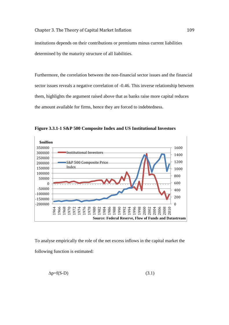
Chapter 3. The Theory of Capital Market Inflation 109
institutions depends on their contributions or premiums minus current liabilities
determined by the maturity structure of all liabilities.
Furthermore, the correlation between the non-financial sector issues and the financial
sector issues reveals a negative correlation of -0.46. This inverse relationship between
them, highlights the argument raised above that as banks raise more capital reduces
the amount available for firms, hence they are forced to indebtedness.
Figure 3.3.1-1 S&P 500 Composite Index and US Institutional Investors
To analyse empirically the role of the net excess inflows in the capital market the
following function is estimated:
p=f(S-D) (3.1)
0
200
400
600
800
1000
1200
1400
1600
-200000
-150000
-100000
-50000
0
50000
100000
150000
200000
250000
300000
350000
19
64
19
66
19
68
19
70
19
72
19
74
19
76
19
78
19
80
19
82
19
84
19
86
19
88
19
90
19
92
19
94
19
96
19
98
20
00
20
02
20
04
20
06
20
08
20
10
$million
Source: Federal Reserve, Flow of Funds and Datastream
Institutional Investors
S&P 500 Composite PriceIndex
Chapter 3. The Theory of Capital Market Inflation 110
Where: p represents a change in stock prices; S is the supply of equity capital and D
is the demand for equity capital, hence (S-D) represents the excess supply (or
purchases) in the capital market.
Before estimating the above equation, it is useful to investigate the linear casual
relationship between changes in stock prices and the excess supply of funds. In order
to do so the Granger causality test is carried out. Granger’s (1969) definition of
causality is ‘a variable Yt is said to Granger-cause Xt, if Xt can be predicted with
greater accuracy by using past values of the Yt variable rather than rather than not
using such past values’ ( Asteriou and Hall 2007). This means that the test uses past
values of the depended variable and the independent variable to determine the
causality relationship between them.
The test requires both variables to be stationary. In order to test for stationary the
Augmented Dickey Fuller (ADF), KPSS and Philips-Perron (PP) tests are used to
detect whether the log level price index and net inflows data are of a stationary form.
The results(shown in Appendix 1, Tables A1-2, A1-3, and A1-4) indicate that the
series is non-stationary so the difference-stationary procedure is used to remove the
trend. The results for the first difference unit root test show that the series no longer
contains a unit root. Hence, the first difference of log price index is stationary and the
series used is said to be integrated of order 1, I (0). The same stationary tests are used
for the net inflows data. As shown in Tables A1-5, A1-6 and A1-7, (shown in
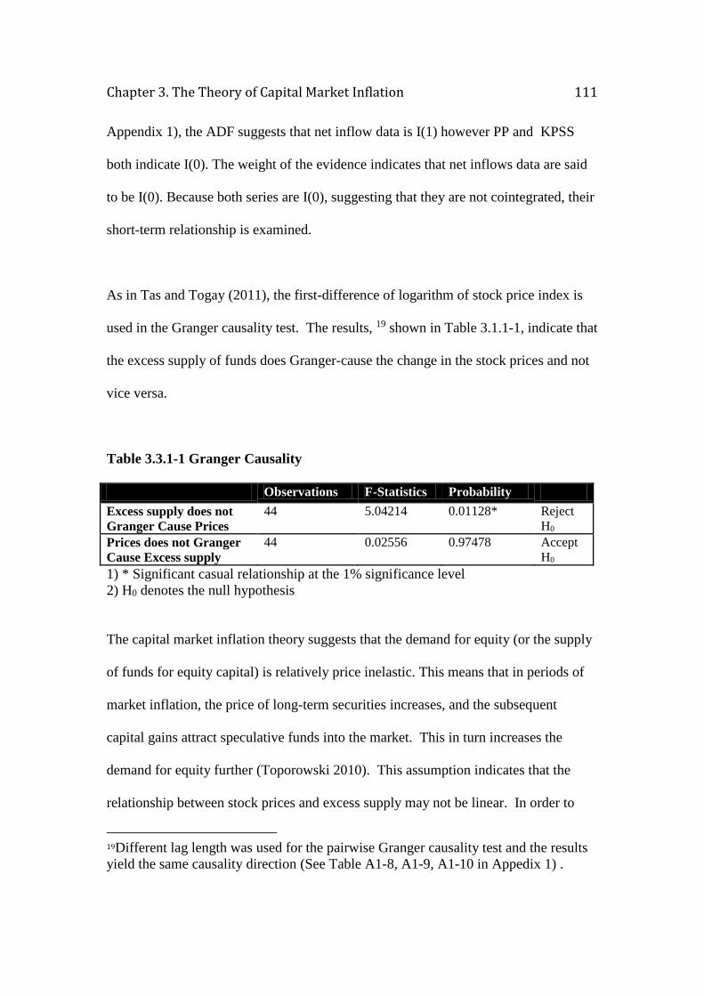
Chapter 3. The Theory of Capital Market Inflation 111
Appendix 1), the ADF suggests that net inflow data is I(1) however PP and KPSS
both indicate I(0). The weight of the evidence indicates that net inflows data are said
to be I(0). Because both series are I(0), suggesting that they are not cointegrated, their
short-term relationship is examined.
As in Tas and Togay (2011), the first-difference of logarithm of stock price index is
used in the Granger causality test. The results, 19 shown in Table 3.1.1-1, indicate that
the excess supply of funds does Granger-cause the change in the stock prices and not
vice versa.
Table 3.3.1-1 Granger Causality
Observations F-Statistics Probability
Excess supply does not
Granger Cause Prices
44 5.04214 0.01128* Reject
H0
Prices does not Granger
Cause Excess supply
44 0.02556 0.97478 Accept
H0
1) * Significant casual relationship at the 1% significance level
2) H0 denotes the null hypothesis
The capital market inflation theory suggests that the demand for equity (or the supply
of funds for equity capital) is relatively price inelastic. This means that in periods of
market inflation, the price of long-term securities increases, and the subsequent
capital gains attract speculative funds into the market. This in turn increases the
demand for equity further (Toporowski 2010). This assumption indicates that the
relationship between stock prices and excess supply may not be linear. In order to
19Different lag length was used for the pairwise Granger causality test and the results
yield the same causality direction (See Table A1-8, A1-9, A1-10 in Appedix 1) .

Chapter 3. The Theory of Capital Market Inflation 112
determine whether their relationship is indeed linear or nonlinear the Ramsey reset
test was used20. The test uses various powers of fitted values of the dependent variable
as proxies for the squared independent variable, to capture any possible non-linear
relationship. This suggests testing for functional form misspecification the following
equation is estimated:
∆𝑝 = 𝛽1 + 𝛽2(𝑆 − 𝐷) + 𝛿12 + 𝛿23 + 휀 (3.2)
The result of the test are shown below:
Table 3.3.1-2 Ramsey Reset Test
Ramsey RESET Test:
F-statistic 3.381462 Probability 0.043486
Log likelihood ratio 6.867831 Probability 0.032260
The p-value associated with the F-statistics, 0.04, is smaller than the 5 percent
significance level; hence the null hypothesis of correct specification is rejected,
concluding that the model is misspecified.
20 Even though the Ramsey Reset test is used to detect nonlinearity, it does not give
any indication of the most appropriate nonlinear model that could be used.
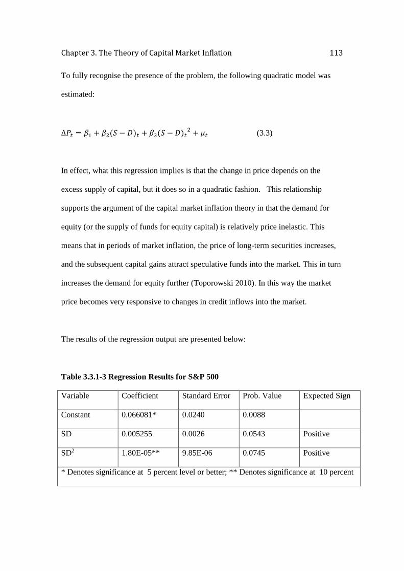
Chapter 3. The Theory of Capital Market Inflation 113
To fully recognise the presence of the problem, the following quadratic model was
estimated:
∆𝑃𝑡 = 𝛽1 + 𝛽2(𝑆 − 𝐷)𝑡 + 𝛽3(𝑆 − 𝐷)𝑡2 + 𝜇𝑡 (3.3)
In effect, what this regression implies is that the change in price depends on the
excess supply of capital, but it does so in a quadratic fashion. This relationship
supports the argument of the capital market inflation theory in that the demand for
equity (or the supply of funds for equity capital) is relatively price inelastic. This
means that in periods of market inflation, the price of long-term securities increases,
and the subsequent capital gains attract speculative funds into the market. This in turn
increases the demand for equity further (Toporowski 2010). In this way the market
price becomes very responsive to changes in credit inflows into the market.
The results of the regression output are presented below:
Table 3.3.1-3 Regression Results for S&P 500
Variable Coefficient Standard Error Prob. Value Expected Sign
Constant 0.066081* 0.0240 0.0088
SD 0.005255 0.0026 0.0543 Positive
SD2 1.80E-05** 9.85E-06 0.0745 Positive
* Denotes significance at 5 percent level or better; ** Denotes significance at 10 percent
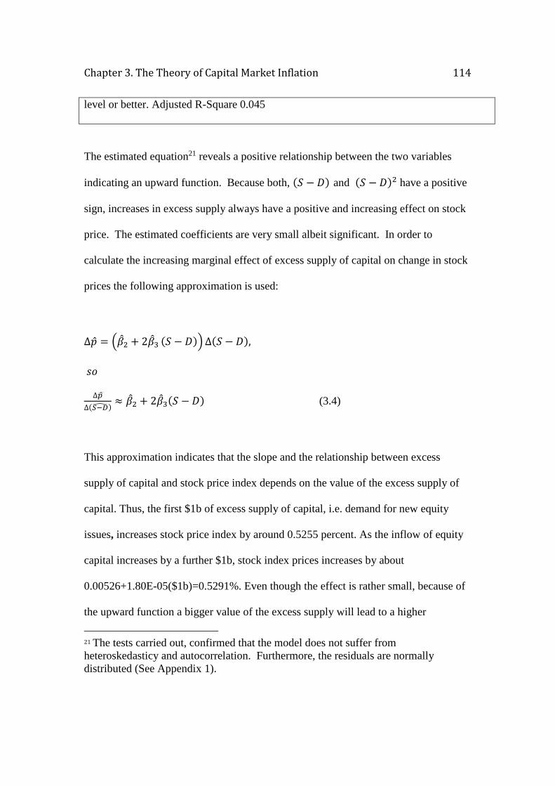
Chapter 3. The Theory of Capital Market Inflation 114
level or better. Adjusted R-Square 0.045
The estimated equation21 reveals a positive relationship between the two variables
indicating an upward function. Because both, (𝑆 − 𝐷) and (𝑆 − 𝐷)2 have a positive
sign, increases in excess supply always have a positive and increasing effect on stock
price. The estimated coefficients are very small albeit significant. In order to
calculate the increasing marginal effect of excess supply of capital on change in stock
prices the following approximation is used:
Δ = (2 + 23 (𝑆 − 𝐷)) ∆(𝑆 − 𝐷),
𝑠𝑜
∆𝑝
∆(𝑆−)≈ 2 + 23(𝑆 − 𝐷) (3.4)
This approximation indicates that the slope and the relationship between excess
supply of capital and stock price index depends on the value of the excess supply of
capital. Thus, the first $1b of excess supply of capital, i.e. demand for new equity
issues, increases stock price index by around 0.5255 percent. As the inflow of equity
capital increases by a further $1b, stock index prices increases by about
0.00526+1.80E-05($1b)=0.5291%. Even though the effect is rather small, because of
the upward function a bigger value of the excess supply will lead to a higher
21 The tests carried out, confirmed that the model does not suffer from
heteroskedasticy and autocorrelation. Furthermore, the residuals are normally
distributed (See Appendix 1).

Chapter 3. The Theory of Capital Market Inflation 115
percentage change in stock prices. Taking the upper quartile value of highest value of
excess inflow of £20.361b the increase of excess inflow to £21.361b increases price
by around 0.6 percent.
Even though the results represent a small change in the price of stock, it is apparent
that the higher the value of net inflows the higher the increase in stock prices, setting
of an inflationary price dynamic as predicted by the capital market inflation theory.
3.4 Capital market Inflation theory applied to the Japanese capital market
Following the same methodology as above, this section applies the capital market
inflation to the Japan capital market. Data is derived from the flow of funds accounts
for the period of 1980-201022.
Data on the Nikkei 225 price index is obtained for the period between 1980-2010,
from DataStream.
Before presenting the empirical analysis conducted over the Japanese stock market, it
is necessary to provide an overview of the structure and regulation of the country’s
22 Due to changes in accounting standards in Japan’s flow of funds, data is available from 1980
onwards. These changes, which took place in July 1999, included not only the changes in the base year, from 1968 System of National Accounts (SNA) to the 1993 SNA, but also restructuring of the
economic sectors in the flow of funds accounts. For example in the flow of funds accounts using the
1968 SNA the household sector was included in the personal sector, which also combined health
insurance cooperatives, mutual aid cooperatives and nonprofits organization. This makes it difficult to
consolidate the data from the new accounting standards to the data using the old accounting standards.
Chapter 3. The Theory of Capital Market Inflation 116
capital market, which has been quite different from the US capital market, prior 1990s
and to a certain extent still remains so. The characteristics of the structure and the
regulatory framework of the Japanese equity market are also important as they could
limit the ability of the model to fully explain the Japanese stock price movements
within a capital market inflation theory framework.
As will be explained in Chapter 6 of this thesis, the Japanese finance sector is known
to have been bank -centered, in which banks have had special relationship with their
main customers. This contrasts with the US financial system which is market-
orientated, and in which the capital markets play a vital role in providing finance.
Japanese capital markets have not always been underdeveloped, in the sense that
banks dominated financing, despite having one of the largest equity markets in the
worlds, based on total value. Prior to the 1930s the Japanese financial system shared
similar characteristics to the postwar US financial system (Hoshi and Kashyap 2001).
The shared feature was the role of the capital market, particularly equity financing, as
opposed to bond and bank financing, in providing finance to industries. Even up
until the 1940s equity financing remained an important source of finance. Allen
(1996) states that during the period 1931-1940, equity issuance provided 31.70
percent of funds, with bonds and loans from private financial institution playing a
smaller role in financing, providing 4.3 percent and 27.3 percent, respectively.
However during this period retained earnings was the major source of funding
providing 37 percent of funds (Allen 1996).
Chapter 3. The Theory of Capital Market Inflation 117
A more recent study conducted by Shabani and Toporowski (2014b), calculates the
net sources of finance for Japanese corporate investment in the period between 1994-
2012, using the flow of funds accounts23. Their analysis shows that internal funds
have remained the most important source of finance for Japanese corporations during
the period under consideration. On the other hand bank finance during the period was
negative, implying that bank finance has experienced net repayments of debt rather
than new funds for investments. Japanese corporations use of equity finance for
physical investment was positive and increased steadily until 2005, but has since
declined turning negative. This suggests that after 2005 the Japanese non-financial
corporate sector has bought back shares and equity. Whereas the evidence on bond
markets do not seem to have been a significant source in providing finance to
Japanese corporations. The overall conclusion of this study could be taken to provide
some evidence that Japan is no longer a bank-based system (Shabani and Toporowski
2014b)
Changes in the structure of the Japanese finance system have their roots in the
financial crises that the country experienced during the 1920s. Japan experienced
three crises during this decade, in 1920, 1923 and a more severe crisis in 1927. In
response to the 1927 crisis a new banking law was implemented which marked the
beginning of the heavily regulated financial system, that was in place until the Big
23 The study employs the same methodology used by Corbett and Jenkinson
(1994,1997) to calculate the sources of finance for physical investment.
Chapter 3. The Theory of Capital Market Inflation 118
Bang reforms in mid 1990s. During the 1930s the Japanese government became
heavily involved in the financial system by means of controlling the allocation of
resources, controlling which assets and liabilities should financial institutions write
off, restricting shareholders’ rights, etc (Allen 1996; Hoshi and Kashyap 2001). The
changes in the regulatory and involvement of the governmental the financial system,
which strengthened banks’ power, led to the creation of the main bank system that has
been in place since the early 1950s. In such system banks have special relationship
with their clients, i.e. firms, in which banks not only are the main debt and equity
holders but also intervene, by means of reducing interest rates, refinancing debt etc.,
when client firms are in financial distress (Allen 1996). The shape of the financial
system in Japan took a different direction from the US. Like Japan, the US radically
changed the regulatory framework of the financial system in the aftermath of the
1930’s crisis. However, in contrast to Japan, the US authorities focused on promoting
a market-oriented financial system. Banks became subject to tighter regulation in an
attempt to prevent banking crisis, with less market intervention. In the US financial
innovation, especially since the 1979s and 1980s, has been key in strengthening
market orientation. But securitisation in Japan did not evolve as it did in the US. The
value of total securitised assets in Japan, at its peak reached just below 2 percent of
GDP, whereas in US in 2007 the value of securitised mortgages was nearly 25 percent
of GDP (The Economist 2011c) (see Chapter 4 for a more detail discussion on the
wide range of financial products innovation that has characterised the US financial
system since the 1970s).
Chapter 3. The Theory of Capital Market Inflation 119
Apart from the main bank system that emerged in the 1950s, the so-called keiretsu24,
which are corporate groups organised around a main bank, is another unique feature
that has characterised the Japanese industrial structure. The main Japanese keiretsu,
known as horizontal25 keiretsu, were Mitsubishi, Mitsui, Sumitomo, Fuyo, Dai-ichi
Kangyo and Sanwa. Within such structures, member firms were closely linked to each
other through cross-shareholding often anchored by commercial banks. Cross-
shareholding is the practice by which firms hold each other’s stock. It is worth noting
here that cross-shareholding was not only conducted by firms belonging to the same
industrial group but also between suppliers and costumers as well as between
creditors and borrowers (Scher 2001). Perhaps the most important relationship for
this research is the bank-corporations cross-shareholding, which is further analysed
below.
The main shareholders of the Japanese banks prior to financial deregulation, that
started in stages during 1980s and culminated in 1996 with the introduction of Big
Bang which was fully implemented in 2001, were insurance companies and corporate
borrowers. Both the double gearing process that had characterised the special
relationship between banks and insurance companies, and the cross-shareholding
system, that characterised the relationship between banks and corporations, could be
24 Up until the 1960s, the business groups that characterized the Japanese economy
were known as Zaibatsu. During the occupation period the zaibatsu groups were
dissolved. However, with the occupation ending, some of the major former zaibatsu
were reformed again into groups now called keiretsu. 25 There are two types of keiretsu: horizontal keiretsu, and vertical keiretsu. The
former is a group of enterprises whereas the latter refer to the supply chain dominated
by a single company. A typical example of a vertical keiretsu is Toyota Corporation
Chapter 3. The Theory of Capital Market Inflation 120
contributing factors in explaining why the capital market inflation theory may not
hold in Japan.
The double gearing process in simpler terms is best described as the process by which
these two types of institution provide each other with capital (Fukao 2003). Japanese
banks issued large amounts of subordinated debt to insurance companies, thus
boosting their Tier II capital. On the other hand, the cash they raised from such
issuance was then used to purchase subordinated debt that insurance companies
issued. Furthermore the money raised by insurance companies was used to finance the
purchase of subordinated debt that banks issued in the first place (Hoshi and Kashyap
2004). Even though the double gearing to some extent declined during 2000-2001, in
the aftermath of the collapse of Chiyoda26, Kyoei and Tokyo Life, in 2001 it still
remained at significantly high levels. For example, as of March 2001, the amount of
bank stocks of the seven Japanese insurance companies totalled to 5.4 trillion yen, and
bank subordinated debt amounted to 5.1 trillion yen. On the other hand the amount of
subordinated debts and the surplus notes of these seven insurance companies held by
Japanese banks were, 1.2 trillion yen and trillion yen, respectively (Fukao 2003).
Cross-shareholding, a process in which banks and corporations hold each other stock,
has also declined since the 1990s. Cross-shareholding between corporations and
banks in Japan not only helped them maintain a strong long-term business
relationship but also positively influenced stock prices (Nagayasu 2003). One reason
26 Tokai Bank suffered 74 billion in losses as a consequence of the failure of Chiyoda
Life in October 2000

Chapter 3. The Theory of Capital Market Inflation 121
for the decline in cross-shareholding during the 1990s was the deregulation of the
financial market, which allowed corporations to access the capital market to raise
finance, independently of their ‘main’ bank. However, Kanaya and Woo (2001), note
that by 2001 Japanese corporate borrowers accounted for half of the total outstanding
shares of banks.
In 1996, after the burst of the bubble in 1990, the Japanese government introduced the
so-called Big Bang reforms as a major step towards financial deregulation. Even
though now the country’s financial and capital markets bear some comparison with
the US, the banking system still accounts for the majority of the financial system
assets. In 2010 Japanese investors holdings of financial assets amounted to a total of
$27 trillion, second highest in the world after the US. However, only 10 percent of the
total is invested in equities. Furthermore, Japanese households still prefer to hold their
wealth in bank deposits. Some 80 percent of household wealth is kept in bank
deposits, with government bonds accounting for 10 percent and investment trust and
other, accounting for 6 percent (McKinsey & Company 2011).
3.4.1 Empirical Results-the case of Japan
As a first step in the analysis on the Japan the inflow contributions of institutions in
the capital market are analysed. The correlation between these contributions and the
stock prices is calculated in order to establish their relationship. As in the case of US,
the data used in the empirical analysis are obtained from the flow of funds accounts
Chapter 3. The Theory of Capital Market Inflation 122
available from the Bank of Japan. However, because of the difference in the flow of
funds accounts between the two countries the following sectors were used to derive
the demand and supply for equity capital in the Japanese capital market:
Institutional investors’ represent purchases of shares and other equity by insurance
companies, including life non-life insurance and mutual aid insurance, and pension
funds, including corporate pensions and other pensions
Household purchases of shares and other equity include purchases of investment
trusts and financial broker dealers
Rest of the world represents only the net purchases of shares and other equity27
The correlation coefficient between institutional investors and Nikkei 225 stock price
index is positive at 0.43. This rather strong positive correlation does not support the
empirical predictions of the capital market inflation theory outlined above. The
positive correlation between Japanese institutional investor and Nikkei 225 stock
price index gives the first hint that the capital market inflation theory may not hold for
the Japanese capital market. The structure and regulation of the Japanese capital and
financial markets, explained above, may be factors that contribute to the empirical
evidence not supporting the capital market inflation theory in Japan. There also
various factors that could explain such inconsistences. For example, the Japanese
27 Contrary to the flow of funds data used for the US, the Japanese flow of funds
accounts does not provide data on the net issues of shares and other equities for the
rest of the world sector. Therefore only their purchases are taken into account in
constructing the database for analyzing the capital market inflation theory with
reference to Japan.
Chapter 3. The Theory of Capital Market Inflation 123
pension fund managers such as trust banks and insurance companies until 1998, were
subject to the 5:3:2 rule, which restricted stock holdings to 30 percent or less, 50
percent had to be invested in secured bonds or loans and 20 percent in the real estate
market. One reason that these restrictions were in place was to make pension funds
investment less risky as well to promote portfolio composition homogeneity
(Weinstein 1997).
In order to test the capital market inflation theory applied to the Japanese capital
market the same methodology as in the case of US is used. Hence, the Nikkei 225
stock price index is estimated as a function of excess supply for equity capital:
p=f(S-D).
As in the case of US, the causality relationship between net inflows and stock price
changes is determined using the Granger causality test is used. As explained above,
the causality test requires both variables to be stationary. The stationary tests
conducted (ADF, PP, and KPSS shown in Appendix 2 ) revel that both variables are
I(0). Table 3.4.1-1 shows the results of the Granger causality test of the first
difference of logarithm of Nikkei 225 stock price index and excess supply. As evident
the results of the test indicate that there is no causal relationship between these two
variables28.
28 The pairwise Granger causality test was also conducted with 2 lags and 4 lags( see
Appendix 2, Tables A2-11 and A2-12.
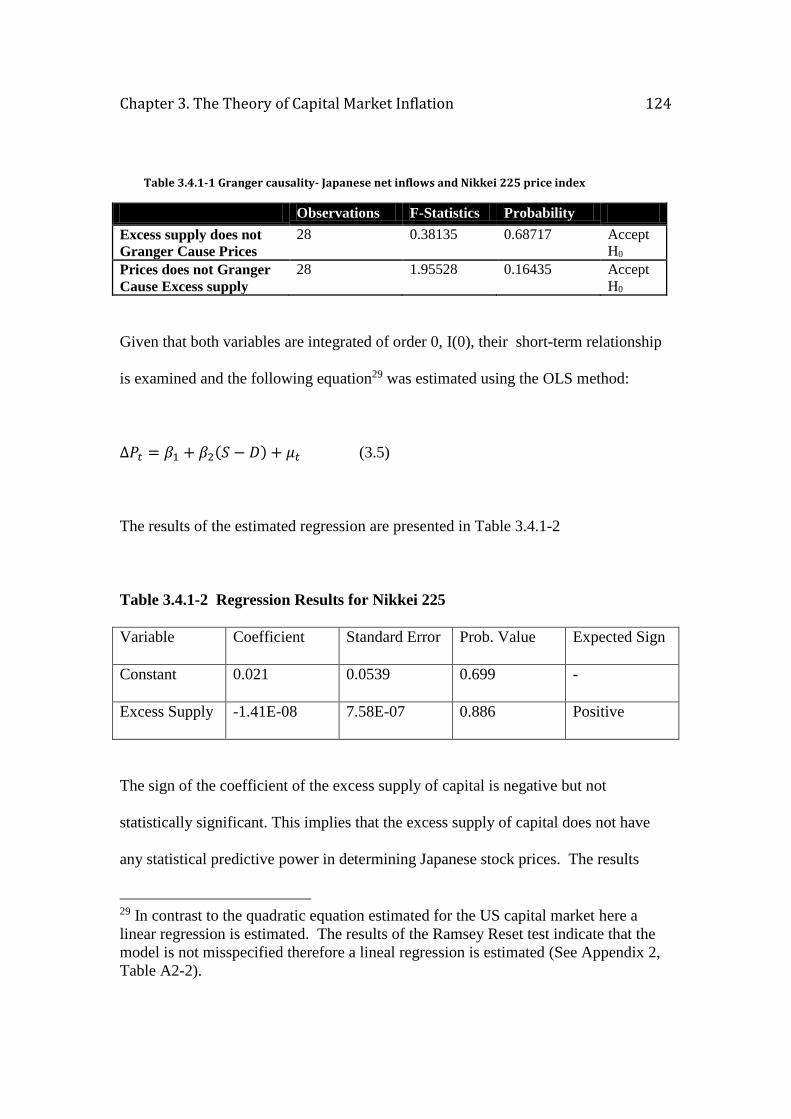
Chapter 3. The Theory of Capital Market Inflation 124
Table 3.4.1-1 Granger causality- Japanese net inflows and Nikkei 225 price index
Observations F-Statistics Probability
Excess supply does not
Granger Cause Prices
28 0.38135 0.68717 Accept
H0
Prices does not Granger
Cause Excess supply
28 1.95528 0.16435 Accept
H0
Given that both variables are integrated of order 0, I(0), their short-term relationship
is examined and the following equation29 was estimated using the OLS method:
∆𝑃𝑡 = 𝛽1 + 𝛽2(𝑆 − 𝐷) + 𝜇𝑡 (3.5)
The results of the estimated regression are presented in Table 3.4.1-2
Table 3.4.1-2 Regression Results for Nikkei 225
Variable Coefficient Standard Error Prob. Value Expected Sign
Constant 0.021 0.0539 0.699 -
Excess Supply -1.41E-08 7.58E-07 0.886 Positive
The sign of the coefficient of the excess supply of capital is negative but not
statistically significant. This implies that the excess supply of capital does not have
any statistical predictive power in determining Japanese stock prices. The results
29 In contrast to the quadratic equation estimated for the US capital market here a
linear regression is estimated. The results of the Ramsey Reset test indicate that the
model is not misspecified therefore a lineal regression is estimated (See Appendix 2,
Table A2-2).
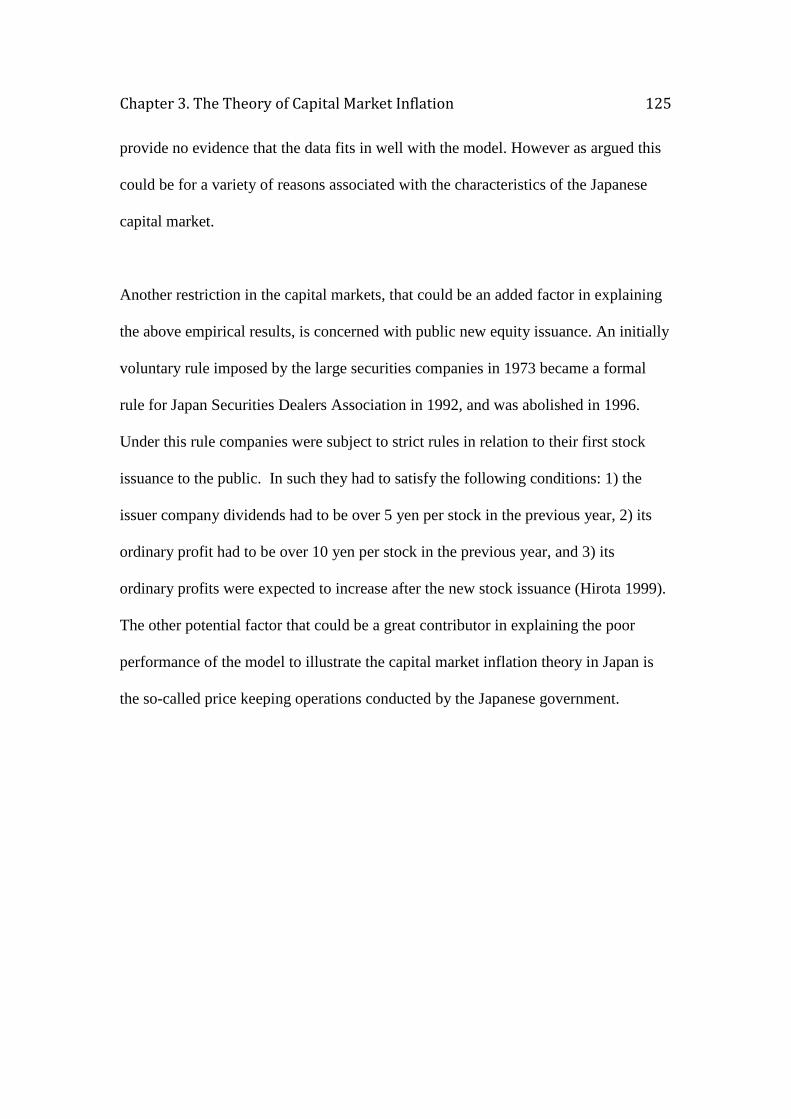
Chapter 3. The Theory of Capital Market Inflation 125
provide no evidence that the data fits in well with the model. However as argued this
could be for a variety of reasons associated with the characteristics of the Japanese
capital market.
Another restriction in the capital markets, that could be an added factor in explaining
the above empirical results, is concerned with public new equity issuance. An initially
voluntary rule imposed by the large securities companies in 1973 became a formal
rule for Japan Securities Dealers Association in 1992, and was abolished in 1996.
Under this rule companies were subject to strict rules in relation to their first stock
issuance to the public. In such they had to satisfy the following conditions: 1) the
issuer company dividends had to be over 5 yen per stock in the previous year, 2) its
ordinary profit had to be over 10 yen per stock in the previous year, and 3) its
ordinary profits were expected to increase after the new stock issuance (Hirota 1999).
The other potential factor that could be a great contributor in explaining the poor
performance of the model to illustrate the capital market inflation theory in Japan is
the so-called price keeping operations conducted by the Japanese government.
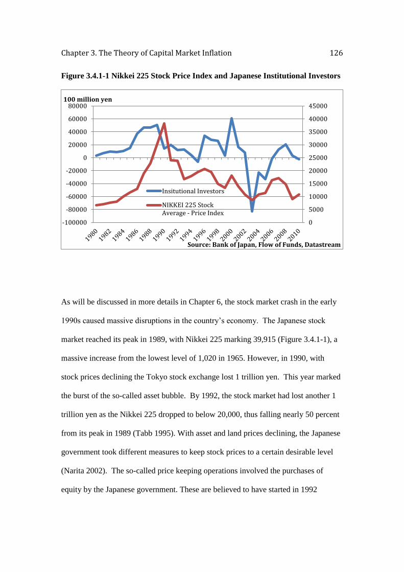
Chapter 3. The Theory of Capital Market Inflation 126
Figure 3.4.1-1 Nikkei 225 Stock Price Index and Japanese Institutional Investors
As will be discussed in more details in Chapter 6, the stock market crash in the early
1990s caused massive disruptions in the country’s economy. The Japanese stock
market reached its peak in 1989, with Nikkei 225 marking 39,915 (Figure 3.4.1-1), a
massive increase from the lowest level of 1,020 in 1965. However, in 1990, with
stock prices declining the Tokyo stock exchange lost 1 trillion yen. This year marked
the burst of the so-called asset bubble. By 1992, the stock market had lost another 1
trillion yen as the Nikkei 225 dropped to below 20,000, thus falling nearly 50 percent
from its peak in 1989 (Tabb 1995). With asset and land prices declining, the Japanese
government took different measures to keep stock prices to a certain desirable level
(Narita 2002). The so-called price keeping operations involved the purchases of
equity by the Japanese government. These are believed to have started in 1992
0
5000
10000
15000
20000
25000
30000
35000
40000
45000
-100000
-80000
-60000
-40000
-20000
0
20000
40000
60000
80000100 million yen
Source: Bank of Japan, Flow of Funds, Datastream
Insitutional Investors
NIKKEI 225 StockAverage - Price Index
Chapter 3. The Theory of Capital Market Inflation 127
(Nagayasu 2003). Estimates show that on November 19, 1992, the Japanese
government purchased about 10 million stocks (Narita 2002). By early 1993, the
amount of the purchases of stocks and bonds by the Japanese government amounted
to one third of all purchases in the market (Tabb 1995). Furthermore, the Ministry of
Finance (MOF), to a certain degree restricted stock selling, whilst encouraging state-
controlled pension funds to spend large amount of money in purchasing stock in order
to boost prices (Tabb 1995). Another informal measure undertaken by the MOF in an
attempt to stop stock prices declining even further, was the request issued to the main
brokers to provide the MOF with the names of the big sellers. Once the news of this
request was spread in the market it is believed to have temporarily increased stock
prices (Tabb 1995).
It is worth noting here that the term ‘price keeping operations’ was a term coined by
the media and not only it was not used by the Japanese government officials but such
operations have also been denied as a practice conducted by them. Therefore the date
in which price keeping operations started or ended still remains unclear (Narita 2002).
Nagayasu (2003) studies the Japanese stock market within the efficient market
hypothesis. Amongst other reasons, the price keeping operations -that is the purchases
of stocks by the Japanese government- is listed as one factor for limiting the
significance of the efficient market hypothesis when applied to Japan. The analysis
provides a graphical representation of the monthly Nikkei stock price movements and
the government purchases of stocks for the period 1992-2002. The arguments
provided in Narita (2002) regarding the uncertainty of when exactly did this
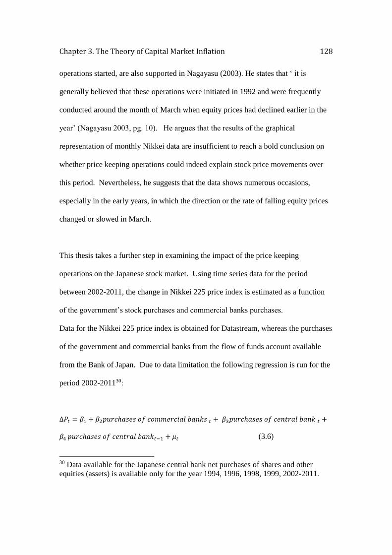
Chapter 3. The Theory of Capital Market Inflation 128
operations started, are also supported in Nagayasu (2003). He states that ‘ it is
generally believed that these operations were initiated in 1992 and were frequently
conducted around the month of March when equity prices had declined earlier in the
year’ (Nagayasu 2003, pg. 10). He argues that the results of the graphical
representation of monthly Nikkei data are insufficient to reach a bold conclusion on
whether price keeping operations could indeed explain stock price movements over
this period. Nevertheless, he suggests that the data shows numerous occasions,
especially in the early years, in which the direction or the rate of falling equity prices
changed or slowed in March.
This thesis takes a further step in examining the impact of the price keeping
operations on the Japanese stock market. Using time series data for the period
between 2002-2011, the change in Nikkei 225 price index is estimated as a function
of the government’s stock purchases and commercial banks purchases.
Data for the Nikkei 225 price index is obtained for Datastream, whereas the purchases
of the government and commercial banks from the flow of funds account available
from the Bank of Japan. Due to data limitation the following regression is run for the
period 2002-201130:
∆𝑃𝑡 = 𝛽1 + 𝛽2𝑝𝑢𝑟𝑐ℎ𝑎𝑠𝑒𝑠 𝑜𝑓 𝑐𝑜𝑚𝑚𝑒𝑟𝑐𝑖𝑎𝑙 𝑏𝑎𝑛𝑘𝑠 𝑡 + 𝛽3𝑝𝑢𝑟𝑐ℎ𝑎𝑠𝑒𝑠 𝑜𝑓 𝑐𝑒𝑛𝑡𝑟𝑎𝑙 𝑏𝑎𝑛𝑘 𝑡 +
𝛽4 𝑝𝑢𝑟𝑐ℎ𝑎𝑠𝑒𝑠 𝑜𝑓 𝑐𝑒𝑛𝑡𝑟𝑎𝑙 𝑏𝑎𝑛𝑘𝑡−1 + 𝜇𝑡 (3.6)
30 Data available for the Japanese central bank net purchases of shares and other
equities (assets) is available only for the year 1994, 1996, 1998, 1999, 2002-2011.
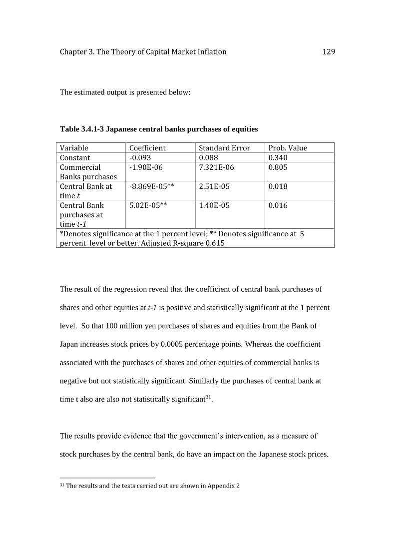
Chapter 3. The Theory of Capital Market Inflation 129
The estimated output is presented below:
Table 3.4.1-3 Japanese central banks purchases of equities
Variable Coefficient Standard Error Prob. Value Constant -0.093 0.088 0.340 Commercial Banks purchases
-1.90E-06 7.321E-06 0.805
Central Bank at time t
-8.869E-05** 2.51E-05 0.018
Central Bank purchases at time t-1
5.02E-05** 1.40E-05 0.016
*Denotes significance at the 1 percent level; ** Denotes significance at 5 percent level or better. Adjusted R-square 0.615
The result of the regression reveal that the coefficient of central bank purchases of
shares and other equities at t-1 is positive and statistically significant at the 1 percent
level. So that 100 million yen purchases of shares and equities from the Bank of
Japan increases stock prices by 0.0005 percentage points. Whereas the coefficient
associated with the purchases of shares and other equities of commercial banks is
negative but not statistically significant. Similarly the purchases of central bank at
time t also are also not statistically significant31.
The results provide evidence that the government’s intervention, as a measure of
stock purchases by the central bank, do have an impact on the Japanese stock prices.
31 The results and the tests carried out are shown in Appendix 2
Chapter 3. The Theory of Capital Market Inflation 130
Therefore, these findings provide an additional and important factor that could
explain why the regression results obtained above show no support of the capital
market inflation theory when applied to the Japanese capital market. Furthermore the
empirical results of the relationship between government intervention and stock price
movements suggests that these purchases offset private sector outflows of credit from
the capital market. So that capital market inflation theory may still hold.
3.5 Concluding Remarks
This chapter has developed a simple model to illustrate the capital market inflation
theory applied to both the US and Japan capital markets. The model is composed by
deriving the demand and supply of capital in the market using flow of funds data for
the period 1964-2010 in the case of US and 1980-2010 for Japan. Even though the
same methodology is used in both countries the estimating regressions differ to reflect
the data properties for each country. Therefore, the US capital market data indicates
that the excess supply of capital has a non-linear relationship with stock prices,
whereas in the case of Japan a liner model was estimated, as statistical tests provided
no evidence, i.e. Ramsey Rest test, of a non-linear relationship. The estimating
results also differ for both countries considered in this analysis. In the case of US,
estimating a quadratic relationship, the results support the capital market inflation
theory in that the price level of long-term securities depends on the inflow of equity
capital into the market. In the case of Japan the model fails to provide any evidence
supporting the theory. It has been argued that there are various factors associated with
Chapter 3. The Theory of Capital Market Inflation 131
the structure and regulation of the Japanese capital market that could be contributing
factors for such results. Furthermore, due to data limitations the time span for the
Japanese capital market is rather short which could limit the ability of the model to
explain stock price movement within a capital market inflation theory.
The empirical evidence on the US capital market is sufficient to validate the
assumptions of the capital market inflation theory. The implications of this validation
are of great importance not only because it provides a framework to better understand
the functioning of the capital markets, but also it provides a basic foundation to
conduct an examination of the impact of the capital adequacy regulation on banks
probability of default.
As argued in Chapter 2 the literature on capital adequacy regulation provides no link
between economic theory and regulatory framework. Capital adequacy regulation is
rather based on intuitions and rule of thumb. Another implication of the empirical
evidence provided in this thesis in supporting the capital market inflation theory is
that it contributes to the asset pricing theory literature by taking into account market
disequilibrium. This original contribution is in contrast to the conventional view of
finance that fails to address the real functioning of the capital markets and the role it
plays in the economy. And it is this linkage that further work in this thesis will
attempt to examine, by using the capital market inflation theory to evaluate not only
the effectiveness of the Basel capital requirements but also the impact that such
regulation has on the business activities of the non-financial sector and thus on the
rest of the economy.
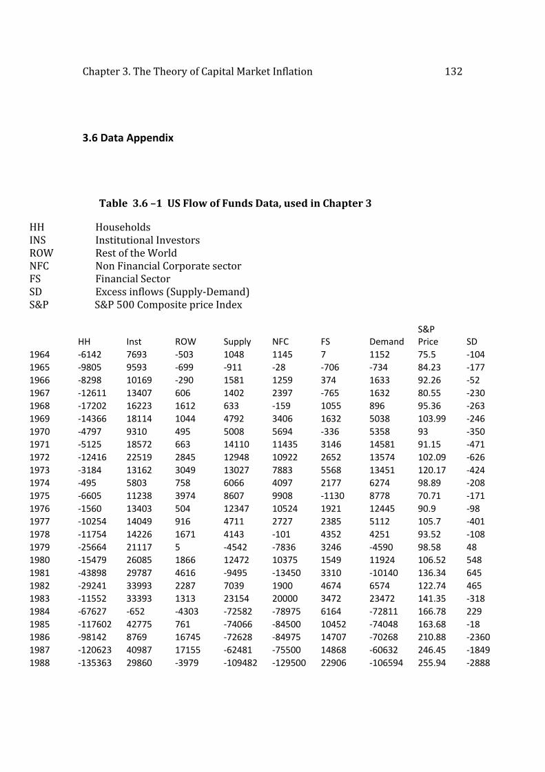
Chapter 3. The Theory of Capital Market Inflation 132
3.6 Data Appendix
Table 3.6 –1 US Flow of Funds Data, used in Chapter 3
HH Households INS Institutional Investors ROW Rest of the World NFC Non Financial Corporate sector FS Financial Sector SD Excess inflows (Supply-Demand) S&P S&P 500 Composite price Index
HH Inst ROW Supply NFC FS Demand
S&P Price SD
1964 -6142 7693 -503 1048 1145 7 1152 75.5 -104
1965 -9805 9593 -699 -911 -28 -706 -734 84.23 -177
1966 -8298 10169 -290 1581 1259 374 1633 92.26 -52
1967 -12611 13407 606 1402 2397 -765 1632 80.55 -230
1968 -17202 16223 1612 633 -159 1055 896 95.36 -263
1969 -14366 18114 1044 4792 3406 1632 5038 103.99 -246
1970 -4797 9310 495 5008 5694 -336 5358 93 -350
1971 -5125 18572 663 14110 11435 3146 14581 91.15 -471
1972 -12416 22519 2845 12948 10922 2652 13574 102.09 -626
1973 -3184 13162 3049 13027 7883 5568 13451 120.17 -424
1974 -495 5803 758 6066 4097 2177 6274 98.89 -208
1975 -6605 11238 3974 8607 9908 -1130 8778 70.71 -171
1976 -1560 13403 504 12347 10524 1921 12445 90.9 -98
1977 -10254 14049 916 4711 2727 2385 5112 105.7 -401
1978 -11754 14226 1671 4143 -101 4352 4251 93.52 -108
1979 -25664 21117 5 -4542 -7836 3246 -4590 98.58 48
1980 -15479 26085 1866 12472 10375 1549 11924 106.52 548
1981 -43898 29787 4616 -9495 -13450 3310 -10140 136.34 645
1982 -29241 33993 2287 7039 1900 4674 6574 122.74 465
1983 -11552 33393 1313 23154 20000 3472 23472 141.35 -318
1984 -67627 -652 -4303 -72582 -78975 6164 -72811 166.78 229
1985 -117602 42775 761 -74066 -84500 10452 -74048 163.68 -18
1986 -98142 8769 16745 -72628 -84975 14707 -70268 210.88 -2360
1987 -120623 40987 17155 -62481 -75500 14868 -60632 246.45 -1849
1988 -135363 29860 -3979 -109482 -129500 22906 -106594 255.94 -2888
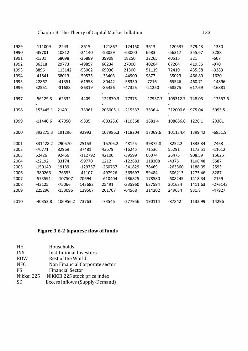
Chapter 3. The Theory of Capital Market Inflation 133
Figure 3.6-2 Japanese flow of funds
HH Households INS Institutional Investors ROW Rest of the World NFC Non Financial Corporate sector FS Financial Sector Nikkei 225 NIKKEI 225 stock price index SD Excess inflows (Supply-Demand)
1989 -111009 -2243 -8615 -121867 -124150 3613 -120537 279.43 -1330
1990 -39701 10812 -24140 -53029 -63000 6683 -56317 355.67 3288
1991 -1301 68098 -26889 39908 18250 22265 40515 321 -607
1992 86318 29773 -49857 66234 27000 40204 67204 419.35 -970
1993 8896 113142 -53002 69036 21300 51119 72419 435.38 -3383
1994 -41841 68013 -59575 -33403 -44900 9877 -35023 466.89 1620
1995 22867 -41351 -61958 -80442 -58330 -7216 -65546 460.71 -14896
1996 32551 -31688 -86319 -85456 -47325 -21250 -68575 617.69 -16881
1997 -56129.3 -62332 -4409 -122870.3 -77375 -27937.7
-105312.7 748.03 -17557.6
1998 -153445.1 21401 -73961
-206005.1 -215537 3536.4
-212000.6 975.04 5995.5
1999 -11440.6 -67050 -9835 -88325.6 -110368 1681.4 -108686.6 1228.1 20361
2000 -392275.3 191296 92993
-107986.3 -118204 17069.6
-101134.4 1399.42 -6851.9
2001 -331428.2 290570 25153 -15705.2 -48125 39872.8 -8252.2 1333.34 -7453
2002 -76771 82969 37481 43679 -16245 71536 55291 1172.51 -11612
2003 62426 92466 -112792 42100 -39599 66074 26475 908.59 15625
2004 -22192 83174 -59770 1212 -122683 118308 -4375 1108.48 5587
2005 -150149 19139 -129757 -260767 -341829 78469 -263360 1188.05 2593
2006 -380266 -76553 -41107 -497926 -565697 59484 -506213 1273.46 8287
2007 -573591 -107507 70694 -610404 -786825 178580 -608245 1418.34 -2159
2008 -43125 -75066 143682 25491 -335960 637594 301634 1411.63 -276143
2009 225296 -153096 129507 201707 -64568 314202 249634 931.8 -47927
2010 -40352.8 -106956.2 73763 -73546 -277956 190114 -87842 1132.99 14296
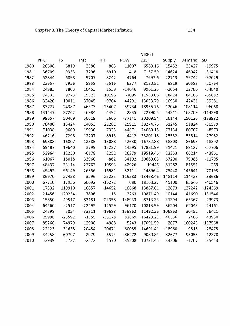
Chapter 3. The Theory of Capital Market Inflation 134
NFC FS Inst HH ROW
NIKKEI 225 Supply Demand SD
1980 28608 6819 3580 865 11007 6560.16 15452 35427 -19975 1981 36709 9333 7296 6910 418 7137.59 14624 46042 -31418 1982 52844 6898 9707 8242 4764 7697.6 22713 59742 -37029 1983 22657 7926 8958 -5516 6377 8120.51 9819 30583 -20764 1984 24983 7803 10453 1539 -14046 9961.25 -2054 32786 -34840 1985 74333 9773 15323 10196 -7095 11558.06 18424 84106 -65682 1986 32420 10011 37045 -9704 -44291 13053.79 -16950 42431 -59381
1987 83727 24387 46373 25407 -59734 18936.76 12046 108114 -96068 1988 131447 37262 46984 4492 2835 22790.5 54311 168709 -114398 1989 99657 50469 50619 2666 -37141 30209.54 16144 150126 -133982 1990 78400 13424 14053 21281 25911 38274.76 61245 91824 -30579
1991 71038 9669 19930 7333 44871 24069.18 72134 80707 -8573 1992 46216 7298 12207 8913 4412 23801.18 25532 53514 -27982 1993 69888 16807 12585 13088 42630 16782.88 68303 86695 -18392 1994 69487 19640 3799 13227 14395 17881.99 31421 89127 -57706 1995 53964 12250 -6178 2252 26279 19519.46 22353 66214 -43861 1996 61067 18018 33960 -862 34192 20669.03 67290 79085 -11795 1997 48437 33114 27763 10593 42926 19446 81282 81551 -269 1998 49492 96149 26356 16981 32111 14896.4 75448 145641 -70193
1999 86970 27458 3296 25235 119583 13468.46 148114 114428 33686 2000 67710 17936 60692 -16272 680 18168.27 45100 85646 -40546 2001 17332 119910 16857 -14652 10668 13867.61 12873 137242 -124369 2002 21456 120234 7896 -15 2263 10871.49 10144 141690 -131546 2003 15850 49517 -83181 -24358 148933 8713.33 41394 65367 -23973 2004 64560 -2517 -22495 12529 96170 10813.99 86204 62043 24161 2005 24598 5854 -33311 -19688 159862 11492.26 106863 30452 76411 2006 25998 -23592 -1355 -35178 82869 16428.21 46336 2406 43930 2007 85266 74979 12908 -4988 -5243 17091.59 2677 160245 -157568 2008 -22123 31638 20454 20671 -60085 14691.41 -18960 9515 -28475 2009 34258 60797 2979 -6574 86272 9080.84 82677 95055 -12378
2010 -3939 2732 -2572 1570 35208 10731.45 34206 -1207 35413
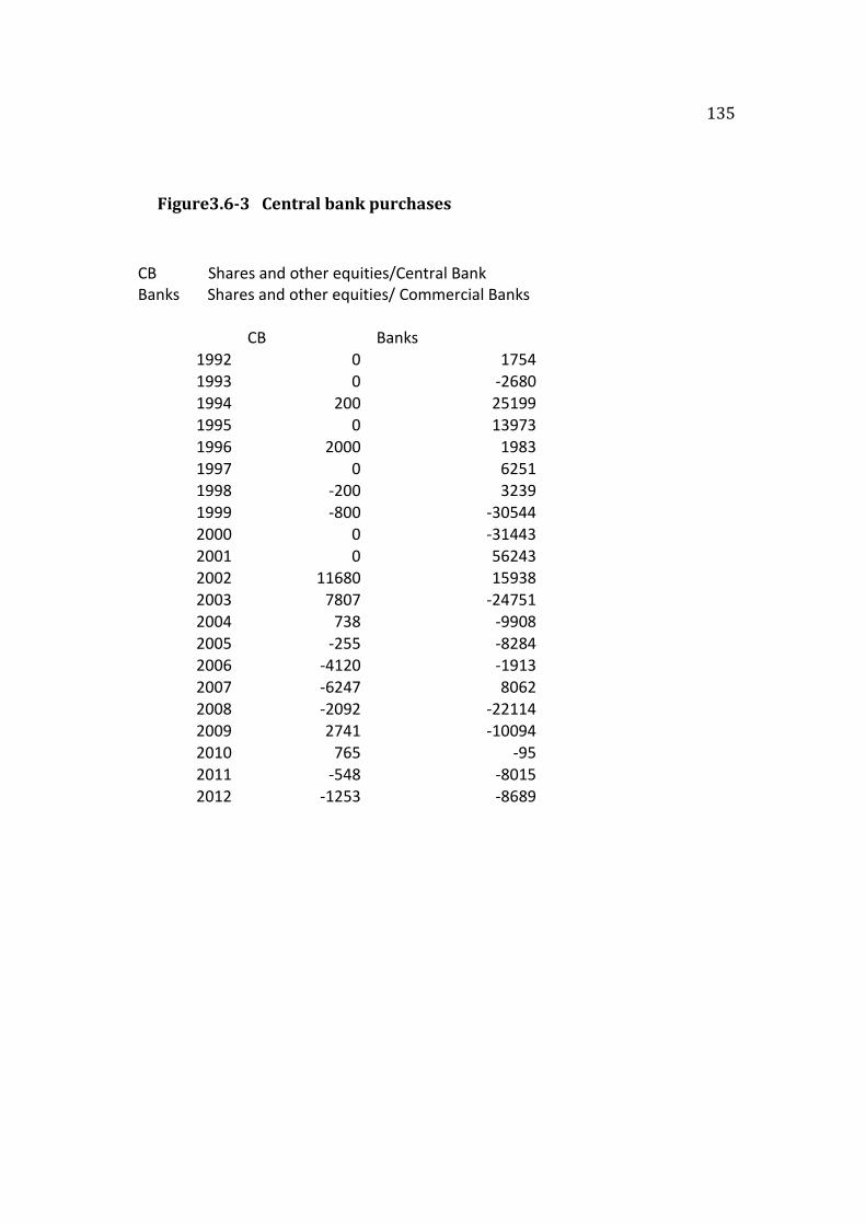
135
Figure3.6-3 Central bank purchases
CB Shares and other equities/Central Bank Banks Shares and other equities/ Commercial Banks
CB Banks
1992 0 1754 1993 0 -2680
1994 200 25199 1995 0 13973 1996 2000 1983 1997 0 6251
1998 -200 3239 1999 -800 -30544 2000 0 -31443 2001 0 56243 2002 11680 15938 2003 7807 -24751 2004 738 -9908
2005 -255 -8284 2006 -4120 -1913 2007 -6247 8062 2008 -2092 -22114 2009 2741 -10094 2010 765 -95 2011 -548 -8015 2012 -1253 -8689
Chapter 4. Shadow Banking 136
Chapter 4. Shadow Banking
The results presented in chapter 3 indicate that under conditions of capital market
inflation firms may be overcapitalised. This has major implications for the
functioning of the capital market. With respect to banks, overcapitalisation, arising
from the imposed Basel capital requirements, increases the riskiness of their assets, as
it crowds out available capital. This chapter argues that by creating a complex and
opaque shadow banking system banks were able to achieve and maintain a reported
overcapitalisation by means of shifting risky assets off balance sheet. The aim of
integrating the shadow banking system in the analysis of capital adequacy regulation
therefore is twofold: firstly, explaining the activities of shadow banks and the
interconnections with traditional banks helps to illustrate the process by which banks
were able to remove risk off balance sheet and report overcapitalisation; and,
secondly, the creation of the shadow banking system not only serves as a cosmetic
manicure for risk in balance sheet but also increases the vulnerability of banks, as
revealed in the latest global financial crisis.
4.1 Overcapitalisation
Chapter 4. Shadow Banking 137
The research in this thesis identifies mainly two processes associated with
overcapitalisation of companies, that has been a rising phenomenon since the 1980s.
The first process is the capital market inflation, which is a generalized phenomenon
reflected in the flow of funds accounts, suggesting that overcapitalisation of the
financial institution or banks, in general increases the riskiness of their assets.
The phenomenon of overcapitalisation is associated with the rise of institutional
investors, such as pension funds and insurance companies, since the 1970s and 1980s.
The accumulation of savings into financial institutions holding long-term financial
assets led to the process of capital market inflation, explained in chapter 3, which
provided higher capital gains from holding shares or common stock. The realised
capital gains are obtained by stock buyers from the market rather the company that
originally issued the stock. This process made equity finance a cheaper and alternative
form of finance, which gave companies an incentive to overcapitalise.
Overcapitalisation is defined as ‘ the issue of equity or common stock in excess of
what is required for the productive and commercial activities of a firm’ (Toporowski
2012). Overcapitalised companies use the excessive raised capital to purchase short-
term liquid assets, thus, increasing the liquidity of their balance sheet. Such assets
could then be used as collateral for short-term borrowing, or balance sheet
restructuring, such as merger and takeover activity. However, the latter activities
could be profitable only if inflation in capital market is (and remains) an on-going
process (ibid).
Chapter 4. Shadow Banking 138
Karwowski and Shabani (2013) analyse the financial operation of US major non-
financial firms for the period between 1994-2012. Using the argument raised by
Toporowski, the paper defines overcapitalisation ‘as a situation in which firms hold
liquidity in excess of what would be needed for productive operations’ (Karwowski
and Shabani 2013). Through a balance sheet examination the results indicate that a
large proportion of the firms in the sample, which are a part of the Dow Jones
Industrial Average, are indeed overcapitalised. Their study also provides evidence
that the identified overcapitalized firms have increasingly engaged in financial
investment.
The second process suggests a different mechanism in that overcapitalisation of a
given bank is also achieved by removing its’ bad assets off balance sheet and their
replacement by superior assets. Such assets may have become available through the
general overcapitalisation of the financial system (more particularly banks). One way
by which banks were able to remove toxic assets off their balance sheet was to
transfer such assets into the shadow banking system. The argument here is that banks
are reporting overcapitalisation rather than being actually over-capitalised. On this
note it is important to stress the differences between absolute and reported
overcapitalisation. The former refers to a situation in which a bank has far more
capital than it needs to conduct it business, where as the latter refers to the process of
reporting overcapitalisation because part of the balance sheet is hidden in the shadow
banking system. This distinction between absolute and recorded overcapitalisation

Chapter 4. Shadow Banking 139
becomes evident in the discussion here on shadow banking system and its
interconnections with the traditional banking system.
4.2 Creation of the Shadow Banking System
The term ‘shadow banking system’ is relatively new in the finance and banking
vocabulary. The financial crisis that unfolded in the summer of 2007, has led many
economists and researchers to look into the causes of such catastrophic event. Their
findings shed some light on the shadow banking system. Even though such a system
(or some of the activities such as securitization) was not newly created but rather had
existed for some time prior to the crisis, the operations and interconnections with the
traditional banking sector grew tremendously to a scale that was relatively unknown
by many, including the regulatory bodies.
Paul McCulley was the first to coin the shadow banking system term in 2007.
He defined the shadow banking system as ‘ the whole alphabet soup of levered up
non-bank investment conduits, vehicles, and structures’ (McCulley 2007). Since then,
the literature provides different definition of the shadow banking system. The
following are some examples:
FSB (2013b)- ‘ credit intermediation involving entities and activities (fully or
partially) outside the regular banking system’ .

Chapter 4. Shadow Banking 140
Adrian and Ashcraft (2012b) – ‘ a web of specialized financial institutions that
channel funding from savers to investors through a range of securitization and secured
funding techniques’
Mehrling et al (2013)- ‘Money market funding of capital market lending-this may or
may not include banks’
Gorton (2010)- ‘ a combination of the repo market and the necessary collateral,
including securitization debt’
This research does not aim to provide a set definition of shadow banking and does not
aim to explain in depth the activities undertaken within the system, but instead will
illustrate how the creation of it allowed banks to move some risky assets off their
balance sheets.
Shadow banks conduct similar activities to traditional banks, by means of engaging in
credit intermediation, maturity and liquidity transformation. However shadow banks
are not subject to the same regulation as traditional banks. Therefore shadow banks do
not have access to liquidity backstops or deposit insurance like traditional banks. In
fact, a common reason given in the literature to explain the extensive engagement of
banks in the shadow banking system is to escape regulation, in particular capital
requirements ( FSB 2012; Gorton 2010; Adrian and Ashcraft 2012a; Pilbeam 2010,
etc).

Chapter 4. Shadow Banking 141
In its simplest form the traditional banking approach has been the same since its
beginnings. Banks accept deposits and use them to make loans. These loans
previously were kept in the banks’ balance sheet till maturity. This has been known as
‘originate and hold’ model. However, as the banking system has evolved in the last 30
years banks have move toward the ‘originate to distribute’ model (Pozsar et al 2012).
This model is best described as a securitization- based credit intermediation process,
explained below.
Over the years the market of the shadow banking system grew to become bigger than
the tradition banking system. As of 2007 the liabilities of the U.S. shadow banking
system amounted to $22 trillion whereas, the liabilities of the traditional banking
system around $14 trillion (Pozsar et al 2010). Because the entities that form the
shadow banking system are not regulated and hence are not required to report to
regulators, it is difficult to have a precise estimate of its size. Given the lack of
transparency of the activities and the opaqueness of the scale of the shadow banking,
Tyson and Shabani (2013) employ a new methodology in an attempt to estimate the
size of UK shadow banking system. The approach makes use of the equal
compensation, which includes both salary and bonuses, to revenue ratio practice
applied by investment banks in all global locations. The ratio disclosed in UK
subsidiary financial statements is assumed to reflect true economic activity in the
location. This assumption is based on the fact that the amount of bonuses given,
calculated as a percentage of revenues, is obtained from internal management
accounts, which use economically correct revenue figures. By contrast the revenue
Chapter 4. Shadow Banking 142
and assets figures disclosed in the financial statement are likely to be distorted by
accounting, tax and regulatory arbitrage. The asset, revenues and bonuses ratios are
calculated using the global accounts, and are then applied to the bonus figure for the
UK’ subsidiaries to imply total UK assets. The figures obtained from each individual
bank included in the selected sample of banks used are summed to give an estimate of
UK off-balance sheet assets of investment banks held in special purpose vehicles
(SPVs). Using five- year average maturity, the level of off balance sheet assets is
estimated to be around $546 billion or 26 percent of on-balance sheet assets. When
combined with the estimated UK’s hedge fund assets of £390 billion, (FSB 2011), the
estimated assets of the UK shadow banking system amounts to over £900 billion
(Tyson and Shabani 2013).
The creation of the shadow banking system comes in parallel with financial
innovation. One the main innovations of the last few decades that has increased
phenomenally and is recognised as a key activity within the shadow banking system is
securitization. Adrian and Ashcraft (2012a) state that securitization as a financial
process has been around since the 1920s but has proliferated in the last 30 years.
Similarly, Pozsar et al (2010), postulate that the shadow banking system was born
some 80 years ago and associate its’ birth with the creation of the government-
sponsored enterprises (GSE). Fannie Mae was the first GSE created by president
Roosevelt as part of the New Deal program in response to the large number of
mortgage defaults during the Great Depression. The main purpose of Fannie Mae was
to provide sufficient and stable funds to mortgage banks in financing housing. In
Chapter 4. Shadow Banking 143
other words it was creating liquidity in the mortgage market, by means of purchasing
banks’ mortgage loans, thus providing banks funds to make new loans.
Fannie Mae was privatized in 1968, and another GSE, Freddie Mac was created in
1970. The two GSEs continued to perform the purpose of their design to buy from
banks, or any other lender, mortgage loans, package them together as bonds,
guarantee them against default, and sell these securities to investors. In its simplest
form this process is known as securitization (CBO 2010).
Following in the footsteps of Freddie Mac and Fannie Mae, banks got involved in
securitization. In a more detail form the process of securitization involves grouping a
variety of assets that generate cash flows, and create a marketable security. The cash
flows act as a guaranty for the security. In other words, securitization transforms
illiquid assets such as loans and mortgages, into liquid assets, such as asset-backed
security (ABS). However, loans and mortgages are just an example of the assets
pooled by commercial banks. Other assets, include, credit cards receivables,
automobile loans, students loans etc. But the common characteristic of all these
assets is that they generate a cash flow, and these are the cash flows of ABS that
investors purchase.
Securitization was taken a step further by financial institutions, by entering into
another process known as re-securitization. In effect this means securitizing a
security that has already been securitized before. These new securities are known as
Chapter 4. Shadow Banking 144
collateralized debt obligations (CDO). For example, banks would set up a special
purpose vehicle (SPV) or special purpose entity (SPE) and sell them the cash flows of
the pool of assets they have packed together. The SPV then slices the pool of cash
flows of the assets into different tranches. These tranches have different risk and
returns: the senior tranches are rated AAA, carry lower risk and thus pay the highest
interest rates; the mezzanine tranches are rated AA to BB, and are risker than senior
tranches; and equity tranches, which are no rated, carry the greatest risk and attract
the highest yield. The process does not end there, but it continues in creating other
securities that are backed by CDO tranches, known as CDO2. The process continues
in creating CDO3 and so forth. Different securities are used as collateral in the
creation of CDOs. When the CDO is formed from packaging loans, is known as
collateralized loan obligation (CLO). Similarly a collateralized bond obligation
(CBO) is created by pooling bonds. When the collateral of the CDO is ABS is known
as ABS CDO.
The first CDO issuance was in 1987 by Drexel Burnham Lambert for the Imperial
Savings Association (Adrian and Ashcraft 2012a) and grew to become one of the
most important activities in modern banking. One of the main advantages of issuing
CDOs by banks is freeing up capital that would have been required to hold if these
loans were kept on their balance sheet (Pilbeam 2010).
Also by creating the SPVs banks were able to eliminate some financial risk. The
SPV is a legal entity set up by another company (the sponsor), a bank in this case, that

Chapter 4. Shadow Banking 145
raise funds to purchase the assets by issuing securities to investors in the capital
markets. The SPVs were created for no other purpose than to conduct these
transactions and they do not to make any business decisions. The entity has no
employees and no physical location and for these reasons is often known as a ‘robotic
entity’. The SPV has another important feature, in that the way it is created allows it
to be bankruptcy remote. That means that in the event of insolvency of the sponsor
bank the SPV will not be affected because its assets are in some way isolated from the
sponsors’ balance sheet. On the other hand in the event of write-downs of assets that
were transferred from the sponsor bank, the SPV is liable to incur the losses.
Therefore, this is a way reducing the financial risk of the sponsor bank (Pilbeam
2010).
According to data published by Lehman Brothers (as cited in Gorton 2010 pg 105),
asset backed commercial paper conduits (ABCPs); special investment vehicles (SIVs)
and SIV-Lites were amongst the main holders of the triple A CDOs tranches. ABCPs
are a form of SPV that are created by large commercial banks, funded through the
issuance of asset backed commercial paper (ABCP). These conduits were originally
set up by banks to provide trade receivables financing to their customers. However,
over the years, in additional to trade receivables, other assets were pooled and used as
collateral, such as student loans, auto loans, credit cards and other various financial
assets. Similarly, an SIV is an off-balance-sheet vehicle and like ABCPs is
bankruptcy remote. SIV issue commercial paper (CP) and medium term notes (MTN)
and ABCP, to fund the purchase of longer-term securities and structured product that
Chapter 4. Shadow Banking 146
earn a higher yield (such as ABS and CDO). The first SIV was designed by Citigroup
in 1988, with the purpose to profit from the spread between short- term and long-term
interest rates (Pilbeam 2010). So in effect an SIV aims to capture the spread between
the lower costs used to fund their liabilities, and higher returns obtained from their
asset portfolio. This way ABCPs and SIVs engaged and specialised in conducting
liquidity and maturity transformation, just like a normal bank does, but as noted with
different means of funding (unlike banks that are funded by deposits, shadow banks
obtain funds through the wholesale money markets).
Even though both SIVs and ABCPs are a form of SPV, they have different structures.
One of the main differences is the liquidity support available to them in the event of a
liquidity crisis. The ABCPs has the advantage of receiving liquidity backstop
provided from highly rated banks (sponsors) as well as some form of credit
enhancement, as additional support. The liquidity support covers 100 percent of their
outstanding ABCPso that sponsors provide funds when the ABCPs is unable to roll
over maturing issues. This way ABCPs are linked to their sponsor banks. Because of
this link, the credit rating that ABCPs receive on their issued commercial paper
depends on the credit rating of the financial institution that provides the liquidity and
credit support, whereas for an SIV the quality of its assets plays a major role on
determining the credit rating it receives (Adrian and Ashcraft 2012a). SIVs did not
enjoy the same liquidity support as ABCPs. The guaranteed liquidity provided by
sponsor banks only covered a part, up to 20 percent of the outstanding ABCP (FDIC
2013). Another major difference between the conduits and SIV is that the former is
Chapter 4. Shadow Banking 147
funded only by means of issuing ABCP, whereas the latter is funded by means of
issuing MTN and other short-term debt.
A shared similarity amongst these vehicles, such as SIVs, SIV-Lites and ABCPs, is
that even though they are bankruptcy remote they are not robotic. They have a
management team and assets are marked to market, unlike SPVs used in the process
of securitization (Gorton 2010). An important point is that these special purpose
vehicles were often not part of the banks that created them, nor were their activities
displayed on their originating bank’s balance sheet (Farhi et al 2009). In this way,
banks were able to increase their balance sheet turnover and therefore extract the
maximum value from their capital.
Another way by which banks were able to reduce their risk was by creating credit
default swaps (CDS). CDSs were first created by JP Morgan and came to existence in
the 1990s (Blinder 2013). A CDS is a credit derivative that has the same features as
an insurance contract. So a contract is reached between two parties, where the seller
party insures the buyer party against any losses arising from the default on a specific
bond (Blinder 2013). In return the buyer party will make regular payments to the
seller party. The CDS market grew significantly in the years preceding the crisis. In
2000 the amount of outstanding CDS was nearly $500 million, and by 2007 it
amounted to nearly $62 trillion (Pilbeam 2010). CDS were an important way in
which banks and shadow banking entities improved the apparent quality of their
assets.
Chapter 4. Shadow Banking 148
Gorton (2010) argues that the activities in the shadow banking system also involve
repurchase agreements. A repurchase agreement (repo) refers to a transaction, which
involves the sale of a security attached with the commitment of the seller to
repurchase the security in the near future at a specified price. Effectively a repo is a
short- term collateralized loan in which an investor32, with a large sum of money, that
wants to invest for a short period of time and earn interest, but is reluctant to deposit
in his bank given the limited deposit insurance, lends to firms and other borrowers in
the repo market and receives securities as collateral (Gorton 2010). The repo market
is also a way in which holders of long-term securities can earn fee income by lending
out their securities. As the repo market evolved, in addition to the usual Treasury
securities, it came to accept a wide range of securities, and structured products such as
ABS and CDOs as collateral. Gorton (2010) states that ‘ the shadow banking system,
is, in fact, a real banking system’ (Gorton 2010 pg. 45). He argues that collateral in
the shadow banking system serves as a form of deposit insurance as opposed to the
deposits in the traditional banking system33 that are insured by the FDIC. Depositors
are institutions with large holdings of cash that opt to invest short term and realize a
return in the form of interest, and lenders are firms that require funds to finance their
business operations. So lenders and borrowers enter in a transaction, which is in effect
repo. A lender (for example a money market mutual fund (MMMF)) lends a large
32 The term investor used here represents the main lenders in the repo market, such as
institutional investors, pension funds, mutual funds, hedge funds, large corporations,
etc. 33 Insurance coverage by the FDIC prior to the crisis of up to $100, 000 per account
has increased to $250,000 (FDIC 2010)

Chapter 4. Shadow Banking 149
sum of money to the borrower (for example an investment bank) and receives some
sort of security as collateral. The investment bank commits to repurchase the same
(or similar) security at a later date for a specified price, and repays all the borrowed
funds plus interest known as the repo rate.
There are mainly two distinguished features of a repo agreement namely:
rehypothecation and haircuts. Rehypothecation is the practise, which gives the holder
of the collateral the right to use it in another transaction. The process can be repeated,
in which the third party that received the collateral can reuse it in another transaction
and so on. The implication of the same collateral being used in number of contracts,
say over the course of one day, is that ‘the collateral has a money multiplier’ (Gorton
and Metric 2012). The other feature of a repo agreement is the degree of
overcollateralization, the difference between the market value of the security used as
collateral and the amount of the loan backed by that security, known as the haircut.
So if borrowed funds amount to $395 million and the collateral has the value of $400
million, the haircut is 1.25 percent. As explained, collateral in repo serves as
insurance and a haircut further protects the buyers (the lender) against default by the
seller (borrower). It is worth noting here that the repo can either be used for
borrowing and lending funds backed by collateral, or for borrowing and lending
securities in exchange for cash. Repos are short-term, usually overnight but most of
them are rolled over on a daily basis. The repo market grew substantially in the last
three decades and even though its size still remains opaque it is estimated to have had
size of the traditional banking system at around $10 trillion (Gorton 2010).
Chapter 4. Shadow Banking 150
The above illustration of a repo transaction conducted directly between the buyer and
the seller of the repo, is known as bilateral repo. Another form of a repo transaction is
known as a tri-party repo and it refers to the use of a third party, a clearing bank, that
handles settlements and managements issues, such as settling the collateral in its own
balance sheet, verifying the quality of the collateral and allocating collateral in a
manner that satisfies the requirement of the lender in respect to eligibility and risk
limitations (Copeland et al 2012). In the US the clearing banks, that act as
intermediaries in the tri-party repo transactions, are the Bank of New York Mellon
and JP Morgan Chase (ibid).
The repo market is a major source of funding for primary dealers, in which they use
repos to finance their inventories of securities. The normal operational practices in
the tri-party repo market, involve the lender and borrower reaching a repo agreement
at the start of the day (Federal Reserve Bank of New York 2010). Later on in the day,
the clearing bank is notified and settles the agreement by simultaneously transferring
cash to dealers (borrowers) and collateral to investors (lenders). The following
morning, the clearing bank unwinds the transaction, whereby, the clearing bank
returns back the securities to dealers and cash back to investors. The unwinding
process is conducted each morning, even for non-maturing repos. By the end of the
business day new repos must be settled, in a process known as ‘rewind’. Because
dealers must finance the securities during the day, that is the time between the
unwound and rewind process, the clearing bank provides financing to dealers, secured
Chapter 4. Shadow Banking 151
by a lien on dealers’ securities. A study conducted by the Federal Reserve Bank of
New York (Copeland et al 2012) , suggests that the exposure of a clearing bank to a
single dealer can routinely be more than $100 billion.
Gorton (2010) and Gorton and Metric (2012) state that the repo market was the main
source of funding for shadow banks or using their terminology ‘ securitized banking
system’. Their definition of securitized banking is associated with the securitization
process in which banks transform illiquid assets, such as mortgages, and any other
loans, into marketable securities that serve as repo collateral. Gorton argues that a
securitization bond, such as ABS and CDOs, that were created by banks and are used
as collateral in the repo market provides a link between the traditional banking and
the shadow banking.
The above introduction of the shadow banking system is just the ‘tip of the iceberg’ in
explaining the complex financial products and the financial chain that was created by
banks and shadow banks. However, it is sufficient to meet the purpose here in
illustrating the ways by which banks were able to shift the risky assets off their
balance sheet and still be overcapitalised. Also, the information provided suffices to
build on an argument that even though bank created products and ways to eliminate
risk off their balance sheet, they also created an opaque and complex system that
played a disruptive role at the heart of the financial crisis.
Chapter 4. Shadow Banking 152
4.3 Shadow Banking and the crisis
Since the onset of the financial crisis in 2007 much research and academic work is
conducted in an attempt to pinpoint the roots of such crisis that had global
implications. A common element in the resulting analysis is the shadow banking
system. As the crisis unfolded in the summer of 2007, causing massive disruptions in
the financial system, not only banks experienced runs (see Chapter 5) but also the
vehicles that these banks created, such as ABCPs and SIVs. During the crisis the
MMMF also experienced a run. The disruptions in the financial market halted
securitization activity (Adrian and Ashcraft 2012b) and seized up the CP market and
the repo market. Following these events the US government came to the rescue by
providing various liquidity facilities, not only for banks but also for those institutions
that are considered as ‘shadow banks’ which are not regulated and hence are not
eligible to government liquidity backstops.
ABCPs and SIVs were the first to be hit at the onset of the crisis in 2007. As
explained above these vehicles borrowed short term in the money market and used
those funds to invest in long -term illiquid assets, such as ABSs and CDOs.
The collapse of the subprime mortgage market caused their assets to deteriorate in
value. Subsequently, there was an investors run on both ABCPs and SIVs creating
difficulties for shadow bank entities. By the end of 2007 the outstanding amount of
ABCP had decreased by around 34 perccent from a peak earlier that year of
approximately $1.2 trillion. Similarly, the SIVs industry, with assets worth $400
Chapter 4. Shadow Banking 153
billion in mid 2007, contracted in size with SIVs outstanding dropping by $100
billion by December 2007 (Gorton 2010).
Sponsor banks which were liable to provide liquidity support to these vehicles, came
to the recue. However, because SIVs received limited liquidity support from their
sponsors, unlike ABCPs, they had to fund their maturing SIVs notes mainly by selling
their assets. Given the deteriorated market conditions, the proceeds from such sales
were not sufficient to refund investors in full (Bank of America 2011).
Faced with these difficulties most sponsor banks provided support to their SIVs, even
though they had no contractual responsibility to do so. In December 2007, Citigroup
announced the bailout of its seven SIVs, by consolidating $49 billion of assets onto its
balance sheet. Other banks such as HSBC and WestLB AG also bailed-out out their
SIVs (Harrington and Hester 2007). However, some SIVs were left to default, with
investors being badly hurt by suffering massive losses. As the crisis erupted further in
2008 SIVs became unviable and by the end of the same year these entities ceased to
exist. In October 2008, Sigma Finance Corp, worth $27 billion, was the last SIV
standing to cease operations (Davis and Sakoui 2008).
Credit default swaps (CDS), which act as insurance against banks/companies defaults,
had served banks well by making their investments look rather sound prior to the
crisis. As investors used CDS to hedge against any potential losses, the banks’
investment were considered safe. However, the use of CDS evolved beyond just
hedging the risk on the purchased bonds. Their use become similar to ‘gambling’, in
Chapter 4. Shadow Banking 154
the sense that bets would be placed on the perceived likelihood of bonds default
(Blinder 2013). But, the purchase of insurance required no ownership of bonds or
loans. This gambling use of CDS is known as “naked CDS”. The use of naked CDS
accounted for nearly 80 percent of the total CDS outstanding in 2008. This is one way
by which product creativity in the financial system created more risk rather than
eliminate it (ibid).
When the crisis took off, it wiped out the value of securities that the insurers, such as
American International Group (AIG), had guaranteed. AIG was the largest derivative
insurer, with a market capitalisation of $95.8 billion as of 2008 (Pilbeam 2010). AIG
offered insurance for a variety of products and in 1998 it offered credit protection in
the form of CDS mainly on mortgage backed securities (MBS) and CDOs. However,
the collapse of the subprime mortgage market caused a massive decline in the value
of CDOs and MBS. Because AIG had a triple AAA credit rating it was not require to
post collateral to its counterparties. This changed when the crisis unfolded: its CDS
counterparties were demanding the firm to post collateral. This was the start of what
became a storm that would bring down AIG. In September 2008 the insurance giant
was downgraded by all three major rating agencies. Even though it managed to post
some (billions of dollars) collateral with its counterparties, it was not enough to
ensure its survival. Unable to raise sufficient funds to meet the further collateral calls
from its counterparties the unregulated firm was nationalized, receiving a whopping
$182 billion bailout money (Blinder 2013).
Chapter 4. Shadow Banking 155
Lehman brother’s collapse had some devastating effect on the financial sector
bringing down with it other financial institutions. One of the financial institutions that
followed suit was the oldest money market mutual fund (MMMF) the Reserve
Primary Fund. The fund’s holding of Lehman’s CP, which amounted to $785 million
in September 2008, became worthless following the failure of the investment bank.
The first MMMF were created in 1971, by the Reserve Primary Fund, and had some
special characteristic that made them relative safe. Their share price was always $1,
which removed any speculation risk, as there are no possibilities of incurring capital
gains, or looses. They normally invested in short-term instruments, such as Treasury
bills, thus their investments were considered to be safe. Amongst these securities,
MMMF started to include in their portfolios CP, given their perceived low riskiness.
However, when Lehman collapsed the firm’s CP, was practically worthless. This
caused the Reserve to be the first fund and for the first time since 199434 to ‘break the
buck’, meaning that the fund’s share declined by 3 cents from their $1 historical fixed
value. As a consequence the Reserve fund faced a large number of redemption
requests from its’ investors. The run followed suit on other money market mutual
funds as investors confidence fell in the industry in the aftermath of the losses that
Reserve suffered. Mutual funds stopped purchasing CP, causing the price of these
securities to drop substantially (Blinder 2013).
34 Community Bankers Mutual Fund was forced to break the buck, following the
bankruptcy of Orange County California in 1994 (Gullapalli et al 2008) and (Condon
2008)
Chapter 4. Shadow Banking 156
In response to a distressed CP market, on September 19, 2008, the Fed created the
Asset Backed Commercial Paper Money Market Mutual Fund Liquidity Facility
(AMLF). The introduction of AMLF aimed to provide support to MMMF to meet
their investors’ requests for redemption as well as to provide liquidity in the ABCP
market (Federal Reserve 2008). AMLF allowed the Fed to provide low rate
nonrecourse loans35 to banks and other financial institutions in order for them to
purchase high quality ABCP from MMMF. However, money markets and ABCP
markets needed further assistance to battle the severe disruptions as the financial
crisis culminated. On October 2008, the Fed established the Commercial Paper
Funding Facility (CPFF) to address the problems in the CP market that were causing
major financing difficulties for US companies. The CP market is vital to US
corporations since it provides the necessary funds to meet any short term mismatch
that arise between payments and receivables. When the CP market dried up, as
MMMF and other investors stopped buying CP and no longer wished to refinance
maturing paper, some of the countries largest companies faced problems in meeting
their financial obligations. In order to stabilize the market the Fed created a SPV, that
was funded by the Federal Reserve Bank of New York, and used the funds to
purchase CP from eligible issuers. The CPFF was closed on 1 February 2010 once the
commercial market become stable (Federal Reserve 2010).
35 Nonrecourse loans are loans that are secured by collateral. However in the event of
default the lender is liable to seize only the collateral on the loans and cannot go after
any other assets that the borrower may possess.
Chapter 4. Shadow Banking 157
During the crisis, apart from the ABCP and MMMF markets, there was also a run on
the repurchase agreement (repo) market. As explained in above lending in the repo
market is conducted with collateral. Gorton (2010) argues that securities used as
collateral in repo transactions before the crisis were ‘information insensitive’. That is,
the value of these securities is known and is immune to adverse selection (Gorton and
Metric 2009). However these perceived information insensitive securities quickly
turned information sensitive as the crisis unfolded. The collateral serves as protection
for lenders, in that in the event of the borrower defaulting the securities used as
collateral can than be sold so that the lender gets his cash investment back. If market
conditions are good then the investor will get back the full amount as reflected in the
value of collateral. However, when market conditions have deteriorated the collateral
might have lost value and hence the investor will not be able to get the full amount
back. Hence he will make a loss. And this is how the debt issued by banks quickly
became information sensitive as investors became nervous about the underlying value
of the collateral as indicated by the increased haircuts. Prior to the crisis usually there
were no haircuts involved in a repo transaction. But this changed during the crisis as
haircuts substantially rose. Gorton (2010) documents this increase and refers to them
as being analogous to withdrawals of deposits in the traditional banking system. He
argues that these withdrawals would trigger a run on banks, as it did in the previous
US banking crisis, prior to the creation of deposit insurance, and the increase in
haircuts triggers a run on the repo market. Gorton’s extensive research on the topic
suggests that it was the run on the repo market that triggered the financial crisis (see
for example Gorton 2010, Gorton and Metric 2009, 2010, 2012).

Chapter 4. Shadow Banking 158
In relation to the tri-party repo market the clearing banks are exposed to the same
risks as the ones that investors face in the above illustration in the bilateral repo
agreements. If dealers are to default than the clearing bank is left with the collateral
in the books, and if the value of the collateral is wiped out or substantially reduced,
than the clearing bank will suffer major losses. However, clearing banks are not
under any contractual obligation to unwind the repo transaction. Lenders became
aware of the fact that clearing banks could potentially decide not to unwind trades and
hence they could be left holding the collateral that needs to be sold. However a quick
sale would cause asset prices to crumble under liquidity pressure. This could
potentially deepen the problems in the market.
In fact during the crisis lenders, worried about dealers financial health, decided not to
roll over the repos, thus they withdrew financing from dealers, despite the collateral
provided by them. In other cases lenders decided to increase haircuts on collateral to
protect themselves against any potential losses arising from a lost value of the
securities held as collateral.
The liquidity strains in the repo market caused a lot of financial distress for many
dealers. For some the consequences were fatal, such as in the case of Lehman
Brothers and Bear Sterns which both failed in 2008. Acknowledging the problems in
the tri-party repo market which were growing rapidly, the Federal Reserve initiated
the creation of the Primarily Dealer Credit Facility (PDCF), ‘to help restore the
orderly functioning of the market and to prevent the spillover of distress to other
Chapter 4. Shadow Banking 159
financial firms’ (Adrian et al 2009, pg 1). The PDCF was established on March 16,
2008, on the same day of the announcement that JP Morgan was to acquire Bear
Sterns (Blinder 2013). Under PDCF, The Federal Reserve Bank of New York was
able to provide funds to primary dealers in exchange for collateral through clearing
banks. So, dealers notified the clearing banks of the overnight funding they needed,
usually by the end of the business day. Once the collateral was received and verified
by the clearing banks the Fed of New York was informed. Upon this notification, in
regards to the loan amount requested and the collateral pledged, the Fed transferred
the funds to the clearing banks to provide credit to dealers (Adrian et al 2009). In
effect the Fed of New York was providing liquidity backstop to primary dealers, that
were not eligible, prior to the creation of PDCF. On September 14, 2008, when
Lehman Brothers was just hours away from bankruptcy, the Fed expanded the use of
the PDCF by accepting a wider range of securities as collateral against the loans it
provided. The expansion of the PDCF was in response to concerns that a possible
collapse of Lehman Brothers could spread the risk to other financial institutions. Once
the market conditions improved the PDCF funds were no longer used and the facility
expired in February 201036.
4.4 Regulation of Shadow Banking
As explained in chapter 2, in response to the latest financial crisis regulation of the
36 Federal Reserve of New York, http://www.newyorkfed.org/markets/pdcf.html
Chapter 4. Shadow Banking 160
banking system has undergone major changes. Basel III introduced new regulatory
measures for banks, which also address the activities in the shadow banking system.
Under the Basel III reforms bans are subject to two liquidity standards: Liquidity
Coverage Ratio (LCR) and Net Stable Funding Ratio (NSFR). Also, in relation to the
new capital requirements standards the credit conversion factor is increased from zero
percent to 20 percent for commitments with an original maturity of one year or less
that are unconditionally cancellable (FDIC 2012).
As argued above, banks were able to shift assets off balance sheet by means of
creating an SPV, such as ABCP and SIVs. In terms of the capital regulation, the
shifting of assets to the SPVs, were treated as sales by regulation and banks were
required to hold risk-based capital only against their contractual exposure to SPVs
(Tarullo 2013).
The crisis shed light on the loopholes in the regulatory framework that gave banks an
incentive to transfer assets into the shadow banking system that allowed them to
adjust their capital requirements at more favourable terms. In 2009 The Financial
Accounting Standards Board (FASB), issued Financial Accounting Standards No. 166
and 167 to amend the accounting rules of certain structured finance transactions
involving SPVs.
The new accounting standards apply to all companies, not just financial institutions,
and it requires them to consolidate those SPVs in which it has control over the most
Chapter 4. Shadow Banking 161
significant activities of these entities as well as when the company has the right to
receive benefits or the obligation to absorb losses from such legal entities (FASB
2009).
Prior to these changes, banks were required to consolidate the assets and liabilities of
ABCP conduits37, but were not required to hold risk based and leverage capital
against these assets. Under the new accounting standards, banking agencies require
banks not only to hold capital against the consolidated assets of their sponsored SPVs,
but also as well as against consolidated securitization transactions (Adrian and
Ashcraft 2012b). Therefore within this new regulatory framework banks ought to
hold higher capital ratios than previously.
The problem in the tri-party repo market during the crisis shed light on the role that
clearing banks play on this market. The difficulties of many dealers during the
financial crisis revealed that clearing banks not only act as agent but are also the
largest creditors in the tri-party repo market. Dealers were heavily dependent on
clearing banks to provide intraday credit to fund their securities. In order to reduce
such dependence the Federal Reserve has undertaken steps, and since 2013 the
amount of intraday credit provided by clearing banks has reduced from 100 percent to
30 percent and it aims to further reduce it to 10 percent by the end of 2014 (Tarullo
2013). Furthermore, the daily unwind process has moved from 8:30 in the morning to
37 Following the failure of Enron, which had sponsored over 3000 off-balance sheet
SPVs (Gorton and Souleles 2006) , the asset and liabilities of ABCP conduits were
required to be consolidated onto balance sheet.
Chapter 4. Shadow Banking 162
3:30 in the afternoon. This reduces the hours of risk that clearing banks are exposed
to, leaving cash investors to hold the risk of the trades during the day. Clearing banks
still provide credit to dealer between the new time of unwinding 3.30 pm till the time
when new trades are settled (Adrian and Ashcraft 2012 a).
However, it is argued that these changes are far from accounting for the systematic
risks associated in the tri-party repo market. The fact that clearing banks still provide
finance to dealers and are exposed to risks, and the use of structure products as
collateral are amongst the most concerned issues raised in the literature (See for
example Adrian and Ashcraft 2012a and Tarullo 2013). In respect to Basel III
reforms, some argue that not only will it not help in stabilizing the financial markets
but it could also increase the size of the shadow banking system. For example, Baur
and Wackerbeck (2013), argue that Basel III has placed traditional banks under more
tight regulation in comparison to shadow banks. This then could lead to financial
institutions to engage more in shadow banking activities. This is likely to be more
profitable for both investors and financial firms due to benefits arising from escaping
the costs associated with the increased capital and liquidity regulatory measures. This
argument goes hand-in-hand with the suggestions given by Gorton and Metric (2010),
which argue that, amongst other reasons, the regulatory costs are a factor that induced
banks to move their assets off balance sheet. They refer to the evidence provided by
Keeley(1988) arguing that when the capital requirements were first imposed in the
U.S., banks with low capital ratios grew relative slower than banks with high capital
ratios. Gorton and Metric (2010), then suggests that if banks are obliged to hold

Chapter 4. Shadow Banking 163
capital ratios to meet the imposed regulatory requirements and when charter value is
low, ‘bank capital will exit the regulated bank industry’ (Gorton 2010 pg 274). And
off balance sheet securitization is a way to such exit.
4.5 Concluding remarks
The creation of the shadow banking system and its interconnections with the
traditional banking system presented in this chapter illustrates neatly how banks were
able to record overcapitalisation without necessary being well-capitalised. Also the
discussion of this chapter shows clearly how the shadow banking system serves as a
cosmetic manicure for risk in reported balance sheets, at the same time are
concentrating risk in the shadow banking system.
The main purpose of the discussion on this chapter is to provide a reinforcing
argument against capital requirements. The root of this argument stems from the
common held view that one reason explaining the rapid growth of the shadow
banking system is associated with capital regulation. Such a system allows banks to
escape regulation, in particular capital requirements. The implication here is that
imposing higher capital requirements on banks may induce complex risk taking, by
means of creating opaque financial products and a complex shadow banking system.
The consequences of such activities were revealed in the latest global financial crisis,
by increasing the vulnerability of the banking system.

Chapter 4. Shadow Banking 164
However the above argument can best be applied only to the US banking sector, as
opposed to the Japanese banking sector, in which shadow banking has not been
significant. In addition this thesis aims to provide an explicit argument, by
empirically examining the impact of capital adequacy regulation on the probabilities
of default of US and Japanese banks, which is presented in the following two
chapters.
165
Chapter 5. Capital Adequacy Regulation and Probability of
default of U.S. banks
Chapter 4 presented a detailed discussion of the creation of the shadow banking
system, which served banks as way to shift toxic assets off balance sheet and record
overcapitalisation. As argued, both the overcapitalisation of banks and the creation of
shadow banks, together with the innovation of complex financial securities, can be
attributed to the capital adequacy regulations set by the Basel Committee.
Subsequently, banks’ vulnerability increased, as evident in the 2007-2009 global
financial crisis. This chapter further examines empirically the consequences of the
Basel capital adequacy regulation on the probabilities of default of US banks, using
the capital market inflation theory, presented in chapter 3. The chapter gives an
overview of the US banking sector and a detailed discussion of the difficulties faced
during the crisis. Section 5.3 explains the methodology used in estimating the
probability of default of US banks for the period 2007-2009. The results, presented
in section 5.4 imply that the higher the Tier I capital ratios the higher the probability
of default, whereas the higher the unweighted risk capital ratio the lower the
probability of default. It is argued that the current risk-weighted capital ratio
requirements only take into account the risk of insolvency ignoring the risk of
illiquidity in the capital market. Section 5.5 discusses the implications of these results
on the system as a whole.
Chapter 5. Capital Adequacy Regulation and Probability of default of U.S. banks
166
5.1 The probability of U.S. banks default
The significance of banking sector instability is now a well-documented phenomenon
in the international financial crisis. Even though signs of an impeding perfect storm
that was about to hit the world economy appeared in late 2006 and early 2007, it was
the 7th August 2007 that marked the start of the crisis. The ensuing credit crunch
caused the collapse of stock markets across the globe, the failure of some of the oldest
and largest financial institutions that threatened the stability of foreign markets. Even
though governments in the most advanced and wealthiest countries came to the rescue
by bailing out banks and other financial institutions the scars that are embedded in the
economy have yet to heal.
One of the warning signs that became apparent in the US banking sector as early as
April 2007 was when New Century Financial filed for Chapter 11 bankruptcy
protection. The company was reported to have been a victim of the deteriorated
housing market conditions (Stempel 2007). Other signs followed when Bear Stearns’
investors learned that their funds invested in two of the firm’s hedge funds had little
value, if any (BBC News 2009).
However, it was on August 7 that made governments around the world realize that the
early signs of an imminent financial crisis were to become reality, and that it would
Chapter 5. Capital Adequacy Regulation and Probability of default of U.S. banks
167
wreak havoc on some of the biggest global banks. On that day, French bank BNP
Paribas froze withdrawals out of the banks’ three mortgage funds, since it was unable
to value fairly some of their assets. Earlier that year, the Bank of England had refused
to provide financial support to one the country’s main savings institutions, Northern
Rock. Following this, the bank experienced a run on its deposits, making it the first
British bank run since 1866 (Blinder 2013). Government efforts to save the institution
proved unsuccessful and on February 2008 it was nationalised. In the same year, the
Swiss government had to refinance UBS bank, the largest in the country and one of
the biggest financial institutions in the world. IndyMac bank was seized by Federal
Deposit Insurance Corporation (FDIC) in June 2008, making it at the time one of the
major collapses in US history. According to reports, the bank failed due to a run by
depositors, which drained the liquidity of the Californian mortgage lender.
However, September 2008 was the time when the US witnessed some of the most
catastrophic events in the country’s financial system. AIG, the world largest insurer,
had been bailed out by the US government along with Freddie Mac and Fannie Mae,
America’s two biggest mortgage lenders. Merrill Lynch was taken over by Bank of
America. During the same period, Lehman Brothers became the first of the ‘too big
to fail’ banks to file for Chapter 11 bankruptcy protection.
Following that, the giant mortgage lender, Washington Mutual was closed down by
regulators and sold to JP Morgan Chase. Over in Europe, the insurance giant Fortis
survived by becoming partly nationalised and Dexia was the second Belgium bank to
be rescued by its government. The latter, considered to be the world’s largest lender
to local governments at the time, became insolvent as a consequence of its US
Chapter 5. Capital Adequacy Regulation and Probability of default of U.S. banks
168
operations losses. RBS, not only the biggest bank in the UK but also with the bigger
loan book than any bank in the world with asset worth £1 trillion, had to be refinanced
by the British government. The British mortgage lender Bradford & Bingley was
nationalised in the same year. In May 2010, the Spanish central bank seized control
over CajaSur, one of the biggest savings banks in the country making it the second
Spanish bank failure since the start of the financial crisis.
The financial turmoil provides evidence that banking collapses could occur on a
massive scale despite the fact that banks were deemed to be too big to fail, well
regulated and well capitalized. Conventional wisdom holds that banks should have
high capital ratios that can sustain unanticipated losses. However the facts provided
above cast questions over the effectiveness of this theory. In a bid to establish the
accuracy of this conventional theory as a remedy to these failures, this chapter
provides empirical evidence on the relationship between banks capital adequacy ratios
and the probability of default. The analysis in this section departs from the capital
market inflation theory put forward in Chapter 3, arguing that rising bank capital
requirements makes them more prone to failure. As previously explained, in
conditions of capital market inflation firms tend to be overcapitalised. The
implications of overcapitalisation provide a foundation to examine the consequences
of bank overcapitalisation issues. Bank overcapitalisation is seen as a result of capital
adequacy regulation set by the Basel Committee. The capital market inflation theory
suggests that under conditions of inelastic equity capital supply, rising capital
adequacy regulation is a way of forcing non-financial firms into debt. The higher the
Chapter 5. Capital Adequacy Regulation and Probability of default of U.S. banks
169
amount of capital held by banks, the lower the quantity available to nonfinancial
intermediaries in the market. Therefore, they are left with no option other than to raise
their needed capital through the issue of debt instruments. The excess debt levels
being held by firms as a consequence of higher banks’ capital regulation requirement
reduces productive investment below what it would otherwise be. The reduced
productive investment also reduces the cash flow of firms and their ability to service
their debt. Therefore, higher capital requirements that aims to avoid banks
unsoundness, encourage firms to reduce their productive investment in fixed capital in
response to their increased indebtedness. Implicitly, excessive firms’ indebtedness
causes a decline in the quality of bank assets, thus increasing their probability of
default.
This thesis employs a logit model to estimate the probability of bank default on a
pooled cross sectional data for US, over the period 2007-2009. Two models are
estimated: a simple logit model using Tier 1 capital ratios and the size of banks
dummy as explanatory variables to predict the probability of bank failure and a
multivariate logit model adding three additional financial variables as proxies for
profitability, asset quality and liquidity. Both models yield results that are in
accordance to the hypothesis of this research that the higher the capital ratios the
higher the probability of default.
5.2 The financial crisis and the U.S. economy
Chapter 5. Capital Adequacy Regulation and Probability of default of U.S. banks
170
During the first decade of the 21st century the US economy went from a period known
as ‘The Great Moderation’ to a period dubbed ‘The Great Recession’. The former
refers to a substantial decline in macroeconomic volatility that characterised the US
economy since the 1980s. The reduced volatility led to widespread perception that
business cycles were a thing of the past. However, 2007 was the start of the worst
financial crisis since the Great Depression in the 1930s. Following the burst of the
housing bubble, the prices of mortgage related securities fell substantially, prompting
huge losses for banks and other financial institutions. For some institutions the
inability to withstand these losses ended their existence. Others survived due to
massive government provision of new capital or were bought by other institutions.
The crisis that unfolded in dimensions beyond what anyone had anticipated, also
severely hit the non-financial corporate sectors. As credit markets froze, the stock
market collapsed, numerous businesses closed down, and with rising unemployment,
the US economy entered into deep recession.
The burst of the housing bubble is commonly considered to have triggered the
financial crisis and the subsequent recession that started in December 2007. The
property market started to show signs of vulnerability in 2006 and 2007, and the rates
of default and late repayment by mortgage holders started to rise significantly
(Murphy and Webel 2008). As a consequence the value of mortgage related
securities asset started to fall, with some having no value at all. The ensuing bank
losses had devastating effects on some of the biggest financial institutions and
brought distress to the whole financial system.
Chapter 5. Capital Adequacy Regulation and Probability of default of U.S. banks
171
Losses in the housing market placed Fannie Mae and Freddie Mac, the two U.S.
biggest mortgage refinancing companies, under strain, threatening their survival. The
government-sponsored enterprises, but owned by shareholders, were created in 1938
and 1970, respectively, to provide sufficient funds to mortgage banks in financing
housing and to keep liquid the market on which mortgage loans could be traded. By
2008 their combined loans were a total of $5.5 trillion (Pilbeam 2010). In the
aftermath of the financial crisis, the US government injected capital totalling $140
billion in an attempt to prevent their collapse. However, the bailout proved not to be
enough to ensure their survival. In September 2008 the two mortgage giants were
placed under government conservatorship.
The crisis culminated on September 15, 2008, when Lehman Brothers filed for
Chapter 11 bankruptcy protection. One of oldest companies of Wall Street, which
had survived the Civil War, the Panic of 1907, and the 1929 stock market crash, was
unable to continue its operations in the aftermath of the financial crisis of 2008. After
running into great financial difficulties, following its heavily exposure both mortgage-
related securities and commercial real estate, the US government refused to rescue the
158 year old firm. Much that followed in the crisis is related to Lehman’s collapse.
The impact of its demise was so severe that for many it defines the start of the
recession the US economy experienced. As will be explained below, after Lehman’s
collapse some of the biggest financial corporations nearly followed suit, but were
however rescued by the government.
Chapter 5. Capital Adequacy Regulation and Probability of default of U.S. banks
172
In response to the financial meltdown, the Emergency Stabilization Act was enacted
on 3 October 2008. The legislation created the Troubled Asset Relief Program
(TARP), which allowed the Department of Treasury to guarantee or purchase up to
$700 billion of toxic assets from troubled financial institutions. On October 13, the
Treasury secretary Hank Paulson gathered the main nine US banks and offered them
each a share of the TARP funds. Banks participation seemed to have been non-
negotiable at that point, in order to avoid exposure of some banks to the market. In
other words, if all banks receive bailout funds, the market would not be able to
distinguish bad banks from good banks. Therefore, it was decided that $25 billion
would go to Citigroup, JP Morgan Chase; $15 billion for Bank of America; $10
billion for Merrill Lynch, Goldman Sachs and Morgan Stanley; $3 billion for Bank of
New York Mellon and $2 billion for State Street Corporation. A further $45 billion
of TARP money was provided to Citigroup and Bank of America in the months that
followed (see below).
In the face of the severe financial distress that the US was experiencing, in February
2010 the US Treasury launched the so-called ‘stress test’ for the largest 19 US bank
holding companies with assets worth more than $100 billion. The test aimed to
evaluate the financial position of these banks, to ensure that they had adequate capital
buffer to withstand any losses and to maintain lending even under more severe
economic conditions. Each bank’s capital was assessed using a two-year ahead
hypothetical adverse scenario. The degree of stress for each bank was determined by
Chapter 5. Capital Adequacy Regulation and Probability of default of U.S. banks
173
assuming possible losses accruing on risky loans, assets and trades in the next two
years. The level of stress was then used to determine the capital buffer position for
each bank, i.e. whether a particular bank needs to increase the capital level or not.
The US Treasury offered capital infusions to those banks that could not raise capital
by themselves, under the Capital Assistance Programme (Marshall 2009). The results
of the stress test were published in May 2009, and revealed that 10 out of the 19
banks needed to raise a further $74.6 billion in capital in order to withstand any
potential losses. In particular, the test indicated that Bank of America needed to raise
as much as $39.9 billion in capital. The other banks with the most significant capital
shortage were: Wells Fargo with $13.7 billion; Citigroup with $5.5 billion and
Morgan Stanley with $1.8 billion. All banks announced plans that would adjust the
capital level that would be in accordance to the stress test (Guha et al 2009).
There have been many suggested factors that caused the financial crisis. Whilst one
factor alone cannot explain the devastating impact, it is commonly believed that the
crisis had multiple causes. Bankers are often blamed for their reckless behaviour
taking too much risk and innovating complex financial instruments but also credit
agencies and regulators bare some responsibility too.
The repeal of Glass-Steagall Act in 1999 has received much attention as one of the
main causes that led to the financial meltdown. The Act was enacted in 1933, in
response to the large number of bank failure during the Great Depression. Preceding
the 1929 stock market crash banks engaged in risky operations through underwriting
Chapter 5. Capital Adequacy Regulation and Probability of default of U.S. banks
174
securities. Their main source of funds used for speculative trading was consumers’
deposits. When the stock market crashed, these deposits were wiped out. As a result
the Glass-Steagall Act came into effect in 1933, separating the activities of deposit-
taking banks from investment banks. The main purpose of this Act was to make
depositors money safer by restricting any connection with the risky activities of
investment banks and created the Federal Deposit Insurance Corporation (FDIC) to
avoid future bank runs (Johnson and Kwak 2010). Commercial banks were under the
protections of the government but subject to tight regulation. The Securities and
Exchange Commission (SEC) was to become the regulatory body for investment
banks.
The Banking Act also enacted regulation Q, which granted power to the Federal
Reserve (Fed) to set interest rate ceilings on savings accounts of banks. During the
1960s the Act was amended to include also savings and loans (S&L) institutions in
addition to commercial banks. However, the 1970s high inflation placed banks under
major difficulties. High inflation leads to high interest rates and because bank loans
were subject to Regulation Q, they were losing money on their fixed rate mortgage
loans. Also, depositors shifted their funds from banks and savings and loans
institutions towards money market funds and Treasury Bills that offered higher rates.
As a consequence, in the early 1980s the saving and loan industry become insolvent.
The impact was milder for banks as they were not exposed to mortgages like the
savings and loans institutions.
Chapter 5. Capital Adequacy Regulation and Probability of default of U.S. banks
175
In the aftermath of the problems faced by the savings and loan industry, the
Depository Institutions Deregulation and Monetary Control Act of 1980 was enacted.
This Act is viewed as the first step towards the deregulation of the US financial
market. Amongst other changes in the regulatory structure for the banking sector and
S&L industry, the Act removed the Fed’s Regulation Q enabling banks to be
competitive by providing higher interest rates on their deposits. Two years later in
1982, the Garn-St Germain Depository Institutions Act was implemented. The Acts
allowed S&L institutions to engage in other risky lending activities rather than
concentrating just on mortgage lending. The regulation changes were placed with the
aim to circumvent problems in the S&L industry. But as it turned out these legislative
actions did nothing but exacerbate the crisis (FDIC 1997). The S&L crisis, led to over
2000-bank failure between 1985 and 1992, and a further 534 failed in 1989.
In 1988, the Basel Accord introduced international capital requirements for
commercial banks. Basel I was implemented in January 1993 and all US deposit
taking banks became subject to the risk-based capital requirements. In order to meet
the capital requirements banks had to adjust their loan portfolios. This resulted in
reduced commercial lending and increased holdings of government securities. This
adjustment was accompanied with the recession of 1990-91. Many suggested that the
credit crunch the US was experiencing was due to the newly introduced capital
requirements. Whilst others viewed the effect of capital requirements as temporary,
ruling out any long-term effect (Furfine 2000).
Chapter 5. Capital Adequacy Regulation and Probability of default of U.S. banks
176
In 2004, Basel II Accord was introduced. The required capital remained the same as
Basel I but Basel II allowed some banks to use their own risk management models to
calculate regulatory capital requirements. The Accord was implemented in stages in
2006 but the US authorities adopted the agreement in 2007 (Pilbeam 2010).
In a response to the financial crisis of 2007-2009, the Basel Committee on Banking
Supervision introduced new regulation standards, known as Basel III, in 2010. Under
the new framework banks are required to hold higher capital ratios in an attempt to
achieve and maintain financial stability. However as stated in chapter 3 the regulatory
framework for capital adequacy requirements set by the Basel Committee provides no
justified economic model nor does it provide a set amount of capital that is sufficient
to protect banks or the banking sector as a whole.
Kuritzkes and Scott (2009) state that before the crisis, the average capital ratios held
by the top 20 US banks was 11.7 per cent. The last reported capital ratios of the five
large US banks38 that either failed or were government-force sold/merger during the
crisis, ranged from 12.3 per cent to 16.1 per cent.
Wachovia’s capital position showed no risk of an imminent failure, prior to its demise
in 2008, as was that of Bear Sterns. Prior to Bear Sterns’ collapse in March 2008, the
chairman of the SEC, Christopher Cox, expressed no concerns about the capital levels
of the firm, stating, “the firm had a capital cushion well above what is required to
38 Bear Sterns, Washington Mutual, Lehman Brothers, Wachovia and Merill Lunch

Chapter 5. Capital Adequacy Regulation and Probability of default of U.S. banks
177
meet supervisory standards” (Norris 2008). Bearn Stearns was known for its heavy
exposure to mortgage-backed securities, and in early March, there were rumours
circulating that the investment bank was struggling. As investors lost confidence, the
firm, which relied heavily in short-term financing such as repos, was unable to raise
funds in the market. The Fed came to the rescue by providing Bear Stearns a $13
billion loan through JP Morgan. However, the loan was not sufficient to ensure the
firms’ survival. Two days later, JP Morgan acquired Bear Stearns for $10 a share.
Following the announcement of the Basel III rules, the US government implemented
the Dodd-Frank Wall Street Reform and Consumer Protection Act. One element of
this Act is the Volcker Rule, which in effect brings back, to some extent, the Glass-
Steagall Act of 1933. The Volcker Rule prohibits commercial banks from engaging in
proprietary trading. That is trading undertaken by banks for their own profit rather
than on behalf of their clients. Therefore commercial banks that are under the FDIC
supervision are banned for proprietary trading, whereas those financial institutions
that are allowed to, will not be liable to government rescue should they need to in the
future. Even though some have argued that these rules are likely to secure a safe
financial system, this dissertation does not address the Volcker Rule but rather
focuses on the impact of the Basel III capital requirements.
5.3 Methodology
Chapter 5. Capital Adequacy Regulation and Probability of default of U.S. banks
178
The most commonly used method for explaining and predicting financial crises are
the early warning system models (EWS). In the empirical literature, there are
essentially two main methodological approaches for constructing EWS models: the
parametric approach and the non-parametric approach. The former approach is the
probability model, such as logit or probit, using limited dependent variables
estimation. The occurrence of a crisis, the dependent variable, is a binary variable,
taking the value one or zero, is estimated as a function of one or more explanatory
variables. The main difference between the logit and the probit model is that the latter
model assumes the cumulative standard normal distribution whereas the logit model
assumes the cumulative standard logistic distribution.
EWS are used not only by academics and private researchers but also by banking
regulatory and supervisory authorities. In the US the evaluation of individual banks
by the regulatory bodies is conducted by means of on-site examination and off-site
surveillance systems (Cole and Gunther 1998). The findings of the on-site
examination determine the rating assigned to banks, based on its financial soundness
and other regulatory criteria. The composite rating, known as CAMELS, is based on
six criteria: capital adequacy, asset quality, management quality, earning ability,
liquidity position and sensitivity to market risk39. In addition to these annually exams
to assess bank performance the regulatory bodies have used off-site monitoring
systems, or early warning systems.
39 Market risk component was added in 1996
Chapter 5. Capital Adequacy Regulation and Probability of default of U.S. banks
179
The CAMELS financial ratios have been used in many empirical researches in
predicting bank failure. Sinkey (1975), was the first to employ the statistical
technique of Multivariate Discriminant Analysis (MDA) to study bank failure using
various financial variables. His analysis examines 110 failed and 110 non-failed US
commercial banks for the period between 1969-1972. His study uses a variety of
financial ratios in order to derive characteristics that distinguish between failed and
non-failed banks in the sample period. The findings suggest that ratios employed to
evaluate bank performance, such as liquidity, capital adequacy and efficiency, are
statistically significant different between the two groups (failed and non-failed banks)
(Sinkey 1975). However, the ability of MDA approach to detect future bank failure is
limited, since it only distinguishes between failed and non-failed banks. Sinkey
(1975) argues that his analysis ‘ represent(s) a preliminary input to the final goal of
developing an early-warning system’ that can enable the prediction of future bank
failure. Martin (1977) was the first to employ a logit analysis to predict bank
failures, and this method is the most commonly used in the literature in predicting
bank failure (Aktas et al 2006).
For the non-parametric approach mainly two models are used to predict financial
crisis: trait recognition model (TRM) and the signal approach. The latter approach,
used to predict both banking and currency crisis involves monitoring the behaviour of
a set of single indicators in periods proceeding and during the crisis. When the
behaviour of a particular variable is assessed as unusual, relative to its normal
behaviour, it is considered to be issuing a warning signal if it goes beyond a threshold

Chapter 5. Capital Adequacy Regulation and Probability of default of U.S. banks
180
value. This threshold value, which expresses an unusual behaviour in a quantitative
manner, is then adjusted to obtain an outcome that balances Type I and Type II errors
(Kaminsky and Reinhart 1999).
Davis and Karim (2008), compare the predictive efficiency of the multivariate logit
model and the signal approach to predict banking crisis using a single dataset. The
analysis estimates the likelihood of a banking crisis as a function of a set of
macroeconomic, institutional and financial variables. Using 105 countries for the
period 1979-2003, their findings favour the multivariate logit model in terms of in-
sample predictive ability. However, the signal approach may be more appropriate
when estimating the probability of a banking crisis for a specific country. This is
because using a common threshold value in the signal approach may not be optimal
since the relationship between the discrete variable (the threshold value) and the
crisis probability is not smooth over the countries in the sample (Davis and Karim
2008).
The other non-parametric approach is the trait recognition model (TRM), a computer
intensive method which aims to identify systematic patterns in the data. This
methodology can detect any irregular performance of the independent variables
included in the model prior to failure/crisis. It stands out from other econometric
models because it does not make any assumptions about the distribution or
independence of the predictor variables. Another unique aspect of the TRM is that
this technique attempts to exploit information from the interaction of variables. The
Chapter 5. Capital Adequacy Regulation and Probability of default of U.S. banks
181
TRM technique has gained popularity in the literature used in predicting bank failure
(Jagtiani et al. 2000).
When TRM is employed there are five steps used in the process of its construction: 1)
the selection of cutpoints for each variable 2) the allocation of binary codes to each
variable 3) constructing a trait matrix for each observation in the sample 4) using this
trait matrix to identify good and bad traits and 5) set classification rules for voting
matrix (for more detail see Kolari et al 2002). The selections of the threshold value
and the classification rules are subject to the judgment of the researcher. The results
depend to a large extend on these decisions which on the other hand could be a source
of bias in the estimation (Gaytan and Johnson 2002).
Kolari et al (2002) compare the predictive ability of the TRM and the logit model for
large US commercial banks over the period between 1989-1992. The authors
estimate the probability of bank failure using both models on a sample containing 100
large banks. Their predictive power was tested using the holdout sample consisting of
50 US commercial banks. Based on classification results the analysis shows that both
models are able to accurately predict in-sample bank failures.
However, the TRM performs better using both one and two year information prior to
collapse, in the holdout sample. Furthermore, the TRM allows the examination of
interaction of different variables, which contain useful information not found on
individual variables in predicting failures. The importance of including variable
Chapter 5. Capital Adequacy Regulation and Probability of default of U.S. banks
182
interactions when predicting bank failures is also highlighted by Jagtiani et al (2003).
Their study tests the efficacy of EWS models in predicting inadequate capitalisation
of US banks. Using the equity to capital ratio as the dependent variable they employ
both logit and TRM analysis to predict incipient financial distress in US commercial
banks as revealed in declining levels of capital ratios. Classifying banks as capital
adequate or capital inadequate, they predict bank capital falling below a specified
adequate level one period ahead. The analysis is based on the assumption that capital
serves as a financial cushion to a financial institution to absorb any unanticipated
losses. Therefore monitoring capital levels predicts the risk of a bank becoming
insolvent and does not predict failure. The results indicate that both of the EWS
models perform well in predicting incipient capital deficiencies a year ahead.
Therefore they argue that both models could be used in the supervisory process in
monitoring bank capital levels.
Inspired by the methodology used in studies conducted by Martin(1977) , Estrella et
al (2000) and others, this research estimates the probability of banks default using a
logit model on a pooled cross sectional data set for the US banks over the period
2007-2009. Two models are estimated in this chapter; a simple logit model using Tier
1 as the sole predictor for probability of default, and year dummies and bank size
dummy variable and a multivariate logit model adding three other financial ratios as
explanatory variables- net interest margin ratio; the ratio of liquid assets to deposits
and short-term funding and the ratio of net charge-off to average gross loans.
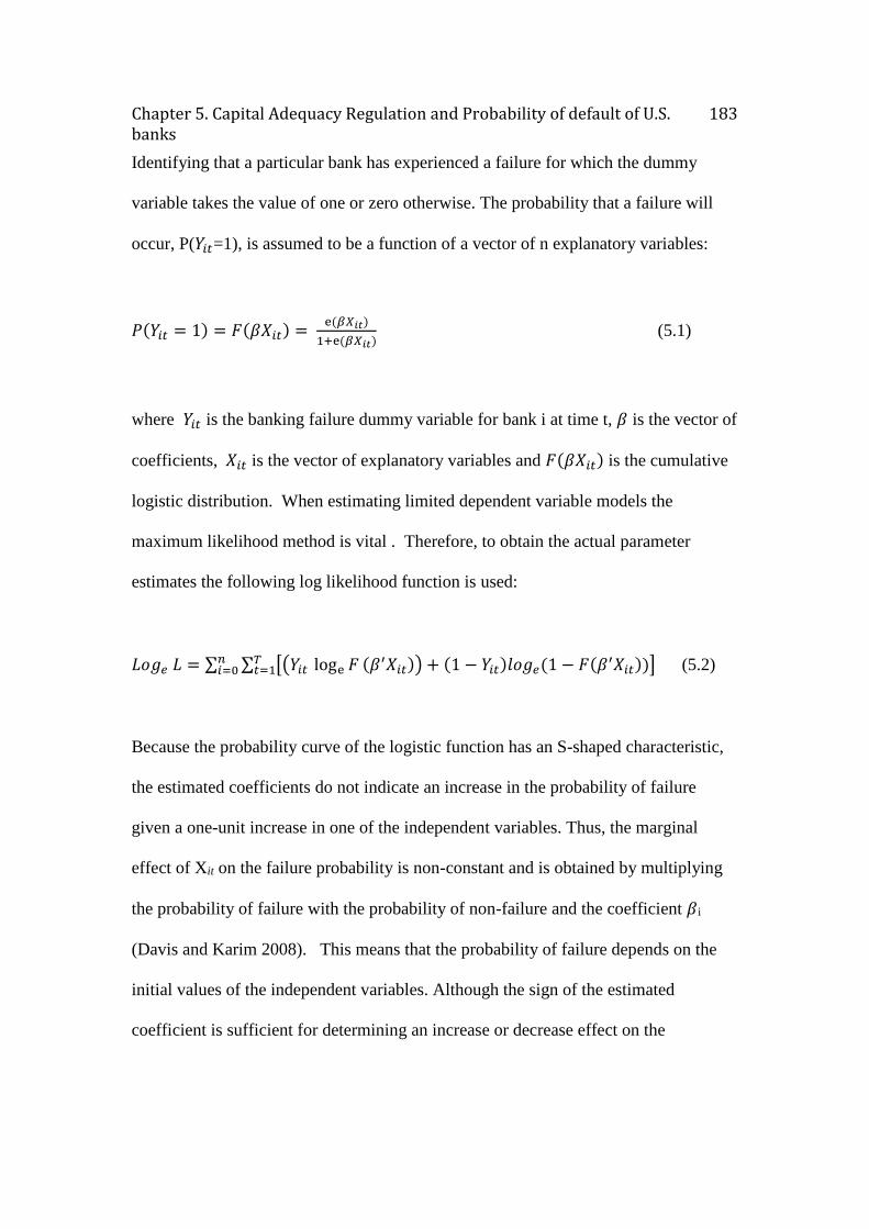
Chapter 5. Capital Adequacy Regulation and Probability of default of U.S. banks
183
Identifying that a particular bank has experienced a failure for which the dummy
variable takes the value of one or zero otherwise. The probability that a failure will
occur, P(𝑌𝑖𝑡=1), is assumed to be a function of a vector of n explanatory variables:
𝑃(𝑌𝑖𝑡 = 1) = 𝐹(𝛽𝑋𝑖𝑡) = e (𝛽𝑋𝑖𝑡)
1+e (𝛽𝑋𝑖𝑡) (5.1)
where 𝑌𝑖𝑡 is the banking failure dummy variable for bank i at time t, 𝛽 is the vector of
coefficients, 𝑋𝑖𝑡 is the vector of explanatory variables and 𝐹(𝛽𝑋𝑖𝑡) is the cumulative
logistic distribution. When estimating limited dependent variable models the
maximum likelihood method is vital . Therefore, to obtain the actual parameter
estimates the following log likelihood function is used:
𝐿𝑜𝑔𝑒 𝐿 = ∑ ∑ [(𝑌𝑖𝑡 loge 𝐹 (𝛽′𝑋𝑖𝑡)) + (1 − 𝑌𝑖𝑡)𝑙𝑜𝑔𝑒(1 − 𝐹(𝛽′𝑋𝑖𝑡))]𝑇𝑡=1
𝑛𝑖=0 (5.2)
Because the probability curve of the logistic function has an S-shaped characteristic,
the estimated coefficients do not indicate an increase in the probability of failure
given a one-unit increase in one of the independent variables. Thus, the marginal
effect of Xit on the failure probability is non-constant and is obtained by multiplying
the probability of failure with the probability of non-failure and the coefficient 𝛽i
(Davis and Karim 2008). This means that the probability of failure depends on the
initial values of the independent variables. Although the sign of the estimated
coefficient is sufficient for determining an increase or decrease effect on the
Chapter 5. Capital Adequacy Regulation and Probability of default of U.S. banks
184
probability of failure the magnitude varies in relation to the slope of the cumulative
distribution function at 𝛽′𝑋𝑖𝑡 (Demirguc-Kunt and Detragiache 1998).
A key element in this model is the construction of the banking failure dummy
variable, which is the dependent variable. To establish which banks enter the
category as failed, information was obtained from various sources. The criteria that a
bank is considered as failed would have had at least one of the four following
conditions: 1) bank that failed for Chapter 11 bankruptcy protection; 2) was seized by
the government or financial institutions; 3) merged with another bank; or 4) is still
operating because of a government bailout which otherwise would not be. For bank
regulatory target capital adequacy ratio the Tier 1 capital ratio is used, obtained from
Bankscope database40. Other variables that are included in the multivariate logit
model are various ratios that intend to determine banks soundness such as liquidity
ratio, asset quality ratio and profitability ratio.
5.3.1 Sample summary
In the estimated logit models, pooled cross sectional data was used for a subsample of
US major banks. All banks are subject to the regulatory capital ratios, which intend to
evaluate banks’ capital strength. Tier 1 capital was used as a measure of capital
adequacy ratio. This is the ratio of a bank’s core equity capital to its total risk-
40 Tier I capital ratio for Countrywide Financial Corporation for year 2007 is obtained
from the company’s annual report, SEC filings, Form 10-k.
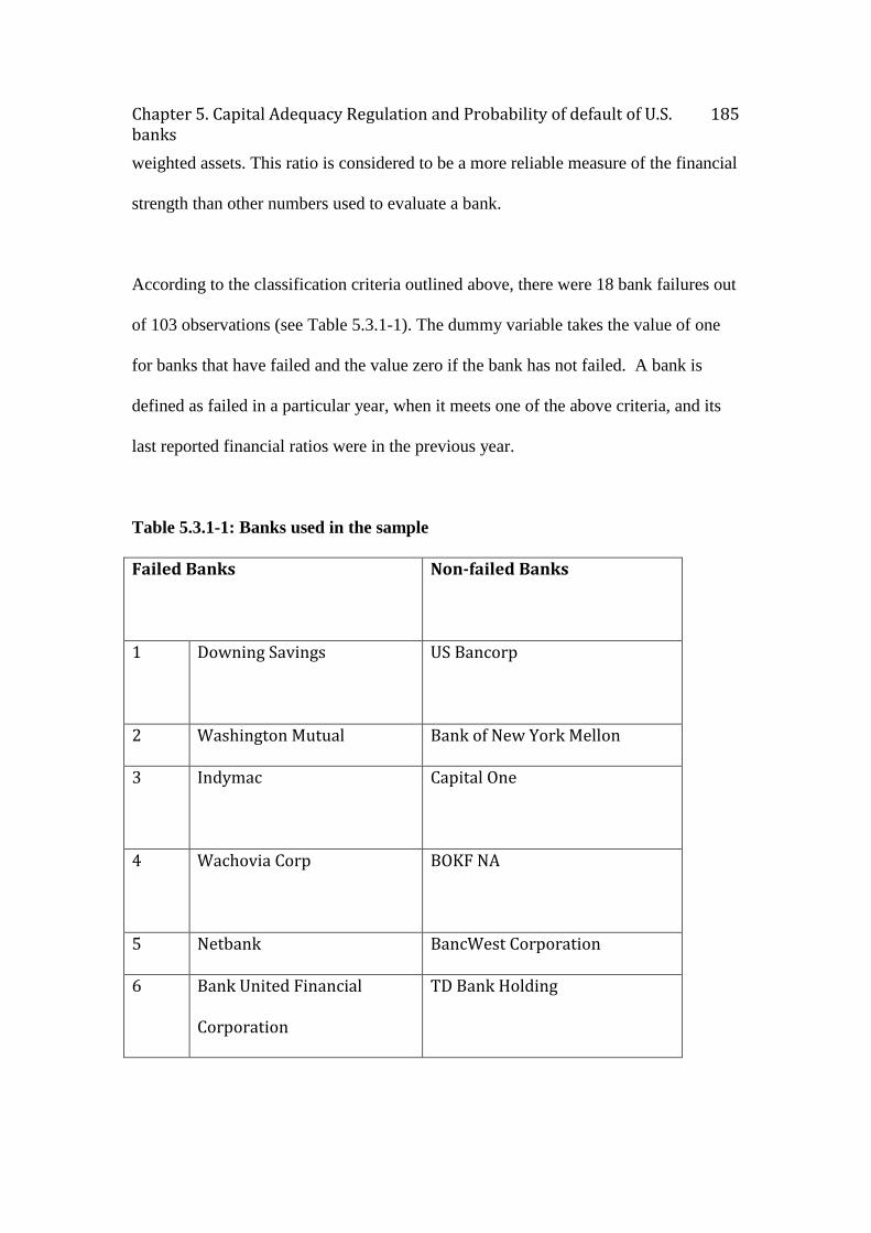
Chapter 5. Capital Adequacy Regulation and Probability of default of U.S. banks
185
weighted assets. This ratio is considered to be a more reliable measure of the financial
strength than other numbers used to evaluate a bank.
According to the classification criteria outlined above, there were 18 bank failures out
of 103 observations (see Table 5.3.1-1). The dummy variable takes the value of one
for banks that have failed and the value zero if the bank has not failed. A bank is
defined as failed in a particular year, when it meets one of the above criteria, and its
last reported financial ratios were in the previous year.
Table 5.3.1-1: Banks used in the sample
Failed Banks
Non-failed Banks
1 Downing Savings US Bancorp
2 Washington Mutual Bank of New York Mellon
3 Indymac Capital One
4 Wachovia Corp BOKF NA
5 Netbank BancWest Corporation
6 Bank United Financial
Corporation
TD Bank Holding
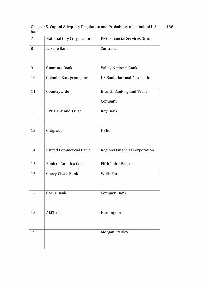
Chapter 5. Capital Adequacy Regulation and Probability of default of U.S. banks
186
7 National City Corporation PNC Financial Services Group
8 LaSalle Bank Suntrust
9 Guaranty Bank Valley National Bank
10 Colonial Bancgroup, Inc US Bank National Association
11 Countrywide Branch Banking and Trust
Company
12 PPF Bank and Trust Key Bank
13 Citigroup HSBC
14 United Commercial Bank Regions Financial Corporation
15 Bank of America Corp Fifth Third Bancorp
16 Chevy Chase Bank Wells Fargo
17 Corus Bank Compass Bank
18 AMTrust Huntington
19 Morgan Stanley
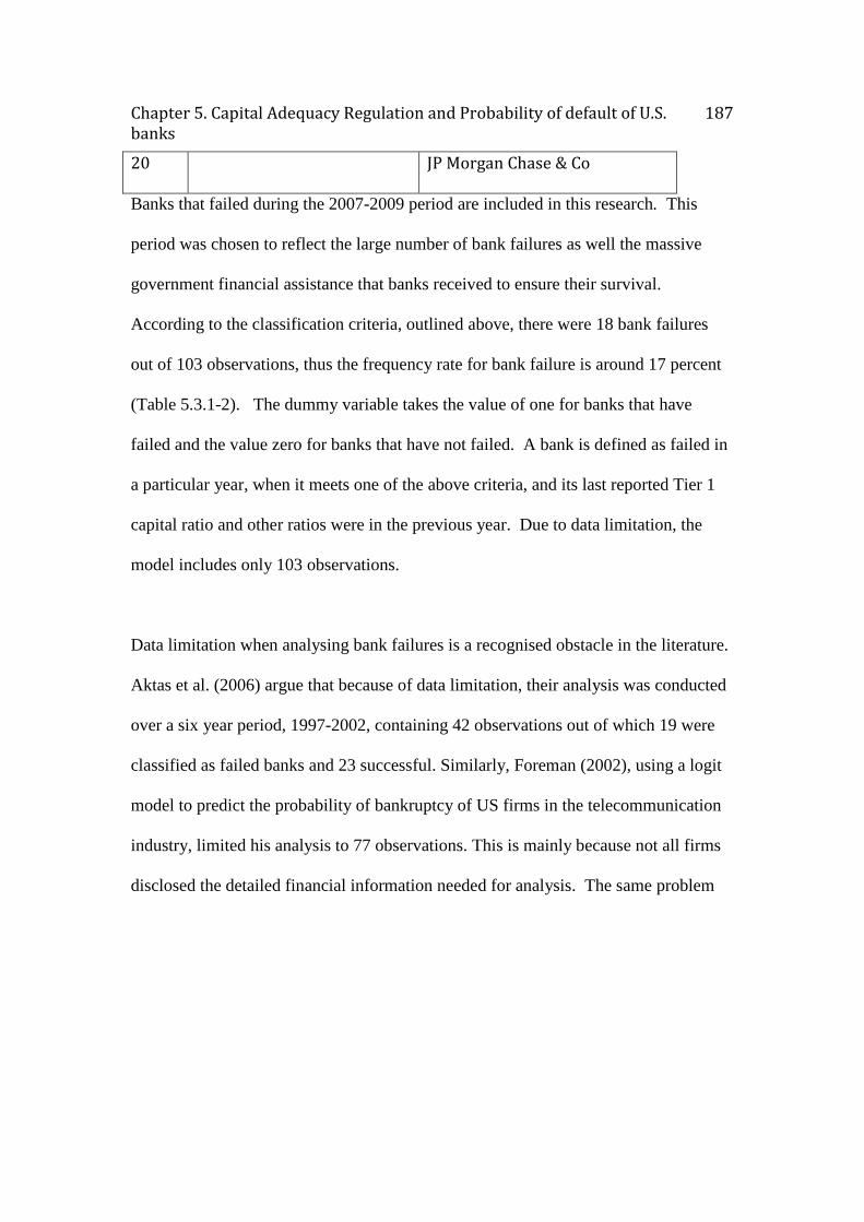
Chapter 5. Capital Adequacy Regulation and Probability of default of U.S. banks
187
20 JP Morgan Chase & Co
Banks that failed during the 2007-2009 period are included in this research. This
period was chosen to reflect the large number of bank failures as well the massive
government financial assistance that banks received to ensure their survival.
According to the classification criteria, outlined above, there were 18 bank failures
out of 103 observations, thus the frequency rate for bank failure is around 17 percent
(Table 5.3.1-2). The dummy variable takes the value of one for banks that have
failed and the value zero for banks that have not failed. A bank is defined as failed in
a particular year, when it meets one of the above criteria, and its last reported Tier 1
capital ratio and other ratios were in the previous year. Due to data limitation, the
model includes only 103 observations.
Data limitation when analysing bank failures is a recognised obstacle in the literature.
Aktas et al. (2006) argue that because of data limitation, their analysis was conducted
over a six year period, 1997-2002, containing 42 observations out of which 19 were
classified as failed banks and 23 successful. Similarly, Foreman (2002), using a logit
model to predict the probability of bankruptcy of US firms in the telecommunication
industry, limited his analysis to 77 observations. This is mainly because not all firms
disclosed the detailed financial information needed for analysis. The same problem
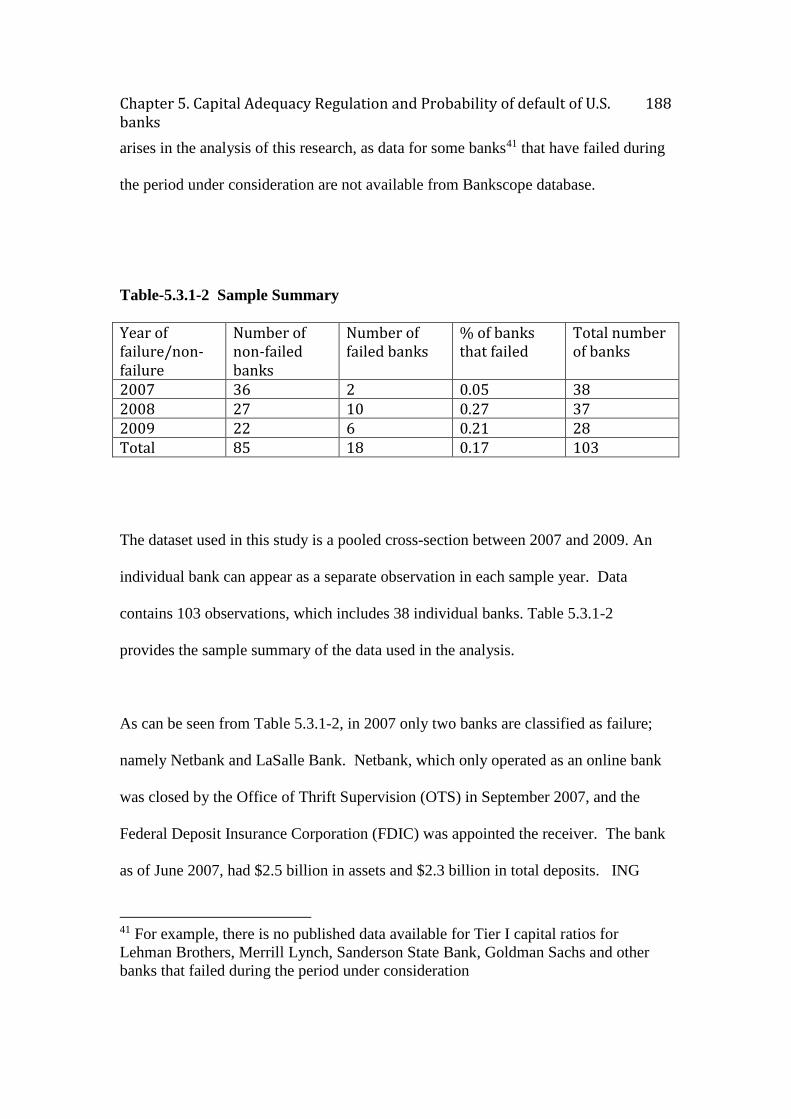
Chapter 5. Capital Adequacy Regulation and Probability of default of U.S. banks
188
arises in the analysis of this research, as data for some banks41 that have failed during
the period under consideration are not available from Bankscope database.
Table-5.3.1-2 Sample Summary
Year of failure/non-failure
Number of non-failed banks
Number of failed banks
% of banks that failed
Total number of banks
2007 36 2 0.05 38 2008 27 10 0.27 37 2009 22 6 0.21 28 Total 85 18 0.17 103
The dataset used in this study is a pooled cross-section between 2007 and 2009. An
individual bank can appear as a separate observation in each sample year. Data
contains 103 observations, which includes 38 individual banks. Table 5.3.1-2
provides the sample summary of the data used in the analysis.
As can be seen from Table 5.3.1-2, in 2007 only two banks are classified as failure;
namely Netbank and LaSalle Bank. Netbank, which only operated as an online bank
was closed by the Office of Thrift Supervision (OTS) in September 2007, and the
Federal Deposit Insurance Corporation (FDIC) was appointed the receiver. The bank
as of June 2007, had $2.5 billion in assets and $2.3 billion in total deposits. ING
41 For example, there is no published data available for Tier I capital ratios for
Lehman Brothers, Merrill Lynch, Sanderson State Bank, Goldman Sachs and other
banks that failed during the period under consideration

Chapter 5. Capital Adequacy Regulation and Probability of default of U.S. banks
189
Bank acquired $1.5 billion in deposits and $724 million of Netbank assets (FDIC
2007). On the same month, Bank of America Corp. announced its plans to acquire
LaSalle Bank from ABN Amro North America Holding Co. LaSalle at the time was
one of the biggest US bank holding companies, and had more than $113 billion total
assets.
In 2008, 10 banks in the sample are identified as failures. They are the following:
Washington Mutual, the third largest mortgage lender prior to the crisis, was seized
by regulators on 26, September 2008. The mortgage bank reported losses that
amounted to $6.3 billion in three successive quarters of 2008, due to deterioration of
the housing market conditions. A few days prior to its demise, the bank’s credit
rating was downgraded from BBB to BB. Following the downgrade, Standard and
Poor credit rating agency reported that ‘ the bank is operating with adequate capital
positions from a regulatory perspective and has demonstrated funding resilience as the
deposit franchise has remained stable’ (Levy 2008). However, Washington Mutual
was suffering from a run on its deposits, losing up to 9 percent as of September 25,
2008(Blinder 2013). On the very same day, the OTC and FDIC closed Washington
Mutual and later sold it JP Morgan & Chase for $1.9 billion (FDIC 2008a).
The decision to close Washington Mutual was in principle governed by the fear that
the run would spread to other banks. However, two days following its closure, the
regulatory bodies of the US banking system faced yet another possible imminent bank
collapse, that of Wachovia. The bank was the country’s fourth largest bank at the
time with assets worth more than $800 billion(Alvarez 2010). Similar to the fate of
Chapter 5. Capital Adequacy Regulation and Probability of default of U.S. banks
190
Washington Mutual, Wachovia was facing a run on its deposits. However, Blinder
(2013) states that the run was rather ‘silent’, meaning that withdraws were conducted
through computers rather than lining up at bank branches. Nevertheless, Wachovia
liquidity was drying up, its stock price was declining sharply and the value of the
banks’ 10-year bonds dropped by more than 60 percent.42
At this point the prospects of Wachovia failing were close to being realised, and thus
the bank was put in the market for sale. Both Citigroup and Wells Fargo were
interested in acquiring Wachovia, and submitted their proposals both requiring FDIC
assistance, albeit different amounts. Citigroup proposed a deal to regulators in which
it offered to purchase Wachovia, in exchange for $2.1 billion in the bank’s stock.
Citigroup was willing to cover the first $42 billion in losses from Wachovia’s loans,
which amounted to about £316 billion, leaving the FDIC to cover any additional
losses. Wells Fargo on the other hand, initially, offered to cover the first £2 billion
losses from a much smaller asset pool, of £ 127 billion. Based on these proposals,
FDIC decided that Citigroup’s proposal was a better deal for them, since its estimated
cost were minimal, whereas, the estimated cost the FDIC would have incurred under
the Wells Fargo’s proposal were between £5.6 billion to $7.2 billion (Blinder 2013).
Therefore, on 29 September 2008, the FDIC announced that Citigroup was to acquire
the trouble Wachovia. However, in a twist of events, the deal with Citigroup broke.
Wells Fargo made a different proposition to the Fed. This time the bid to acquire
Wachovia did not require any federal assistance. On October 3, Wachovia’s board
42 Blinder (2013) reports that the price of Wachovia’s 10-year bonds dropped form 73
cent on the dollar to 29 cents
Chapter 5. Capital Adequacy Regulation and Probability of default of U.S. banks
191
decided to accept Wells Fargo deal because it offered $6 per share more than
Citigroup’s offer. FDIC announced the agreement on the same day, which resulted
in Citigroup’s stock dropping by 18 percent (Blinder 2013). The bank had already
received $25 billion of TARP money in October but its financial position remained
weak and needed further government assistance. On 23 November 2008, it was
announced that the Fed, FDIC and the Treasury had decided to inject a further $20
billion into Citigroup. The bailout was arranged under the conditions that the
government would purchase $27 billion of preferred stock on which Citigroup was
liable to pay an 8 per cent dividend. Furthermore, Citigroup would absorb the first
$29 billion in losses on the $306 billion portfolio, plus 10 per cent on any potential
losses. The rest was left to the FDIC, the FED and the Treasury to absorb.
Another bank that was still struggling for survival even after receiving $25 billion
TARP funds in October 2008 was Bank of America Corporation, the saviour of
Merrill Lynch. In December 2008, the Fed and the Treasury were informed that Bank
of America was in trouble due to the mounting losses of Merrill Lynch. In mid
January 2009, the bank received a further $20 billion of TARP money, on nearly the
same condition as the Citigroup’s bailout. CNN Money reports that regulators agreed
to inject capital in return for preferred stock carrying an 8 per cent dividend (Goldman
et al 2009). However, the pool of toxic assets that were guaranteed by the
government totalled $118 billion, a much smaller amount of Citigroup’s pool of
portfolio assets. Bank of America was liable to absorb the first $10 billion and a
Chapter 5. Capital Adequacy Regulation and Probability of default of U.S. banks
192
further 10 per cent on any additional losses, leaving the Treasury and the FDIC to
absorb the rest.
The demise of IndyMac in 2008 was considered at the time the third largest bank
failure in the US history43. In the summer of 2008, the weak financial position of the
mortgage bank was pinpointed by Senator Charles Schumer. The senator expressed
his worries over the troubled bank in a letter addressed to regulators. In the days that
followed the bank experienced a run on its deposits. A total of £1.3 billion deposits
were withdraws 11 days after the fears over its solvency were raised by the senator
(Paletta and Enrich 2008). IndyMac was seized by federal regulation in July 2008.
The FDIC temporarily ran the bank, under a new name, IndyMac Federal Bank, FSB,
until it sold it to OneWest Bank, FSB in March 2009 (FDIC 2009a).
BankUnited Financial Corporation, the parent company of BankUnited FSB, the
largest bank headquartered in Florida, raised fears of being on the verge of collapse,
after failing to comply with the Securities and Exchange Commission (SEC)
mandatory rules in disclosing their fiscal accounts for 2008. The company also
received notification from Nasdaq Stock Market, indicating that the inability to file its
accounts on time threatened its continued listing. BankUnited company was expected
to have suffered losses of at least $327 million, in the last quarter of 2008 alone
(Hielscher 2008). In March 2009 it filed for Chapter 11 bankruptcy (Gale 2009).
43 The failure of Continental Illinois in 1984, with assets worth $40 billion was
considered the largest failure in US history, followed by the collapse of the American
Saving & Loan Association in 1988.
Chapter 5. Capital Adequacy Regulation and Probability of default of U.S. banks
193
Because its last available accounts are in 2007, and because of the actual distress the
bank experienced in 2008, its failure is recorded in 2008 in the sample data used in
this research.
Downey Savings &Loan after suffering major losses in late 2007 and early 2008,
failed on November of the same year. FDIC announced that U.S. Bank, National
Association acquired all Downey Savings assets worth $12.8 billion as of September
30, 2008. In November 2008, U.S. National Association also purchased PFF Bank
and Trust, which was closed by regulators on the same month (FDIC 2008b) .
Countrywide Financial Corporation the largest US mortgage lender at the time was
rescued by the Bank of America in January 2008. The rescue came after the giant
mortgage lender run into financial difficulties and lost substantial market value, as
economic conditions in the mortgage market worsened. Bank of America agreed to
purchase the company for around $4 billion (Mildenberg 2008)
National City Corporation sold First Franklin, one the country’s main subprime
lenders, to Merrill Lynch in 2006. Since then the bank experienced major financial
difficulties and in 2008 applied for federal bailout funds but was rejected (Engel and
McCoy 2011). In October of the same year National City Corporation was acquired
by the PNC Financial Services Group.
Capital One Financial Corp. announced in December 2008 the purchase of Chevy
Chase for $445 million in cash and $75 million in stock (Dealbook 2008).
Chapter 5. Capital Adequacy Regulation and Probability of default of U.S. banks
194
In August 2009, the OFS closed Guaranty Bank, and its receiver FDIC immediately
arranged its sale to Spanish bank BBVA Compass. As of June 2009, the bank had
assets of around $13 billion out of which BBVA Compass purchased $12 billion, the
remaining assets were held by FDIC (FDIC 2009b). On the same month, August
2009, Colonial BancGroup filed for bankruptcy Chapter 11 after its banking units was
closed by the Alabama State Banking Department, naming the FDIC its’ receiver.
FDIC then quickly facilitated its sale to Branch Banking and trust (BB&T) (FDIC
2009c).
The 120th bank failure in 2009 was United Commercial Bank, which was seized by
federal regulators in early November that year (Campbell 2009). FDIC announced
later that East West Bancorp acquired all the United Commercial’s deposits.
Corus Bank was seized by the government in September 2009, and was immediately
sold to MB Financial Bank. In December of the same year, the OTS closed AMTrust
bank, and was later sold to New York Community Bank (FDIC 2009d).
5.3.2 Descriptive Statistics
As in Bunn and Redwood44 (2003) the explanatory variable, Tier I capital ratio, is
obtained from bank reported accounts in the year preceding the year of non-failure
44 Although they estimate a probit model to examine the determinant of failure of both
individual public and private UK’s companies, the same methodology can be applied
to the logit model as the only difference between the two models is that the probit
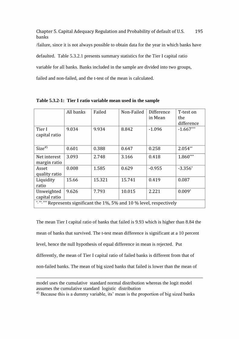
Chapter 5. Capital Adequacy Regulation and Probability of default of U.S. banks
195
/failure, since it is not always possible to obtain data for the year in which banks have
defaulted. Table 5.3.2.1 presents summary statistics for the Tier I capital ratio
variable for all banks. Banks included in the sample are divided into two groups,
failed and non-failed, and the t-test of the mean is calculated.
Table 5.3.2-1: Tier I ratio variable mean used in the sample
All banks Failed Non-Failed Difference in Mean
T-test on the difference
Tier I capital ratio
9.034 9.934 8.842 -1.096 -1.667***
Size45 0.601 0.388 0.647 0.258 2.054**
Net interest margin ratio
3.093 2.748 3.166 0.418 1.860***
Asset quality ratio
0.008 1.585 0.629 -0.955 -3.356*
Liquidity ratio
15.66 15.321 15.741 0.419 0.087
Unweighted capital ratio
9.626 7.793 10.015 2.221 0.009*
*, **, *** Represents significant the 1%, 5% and 10 % level, respectively
The mean Tier I capital ratio of banks that failed is 9.93 which is higher than 8.84 the
mean of banks that survived. The t-test mean difference is significant at a 10 percent
level, hence the null hypothesis of equal difference in mean is rejected. Put
differently, the mean of Tier I capital ratio of failed banks is different from that of
non-failed banks. The mean of big sized banks that failed is lower than the mean of
model uses the cumulative standard normal distribution whereas the logit model
assumes the cumulative standard logistic distribution 45 Because this is a dummy variable, its’ mean is the proportion of big sized banks
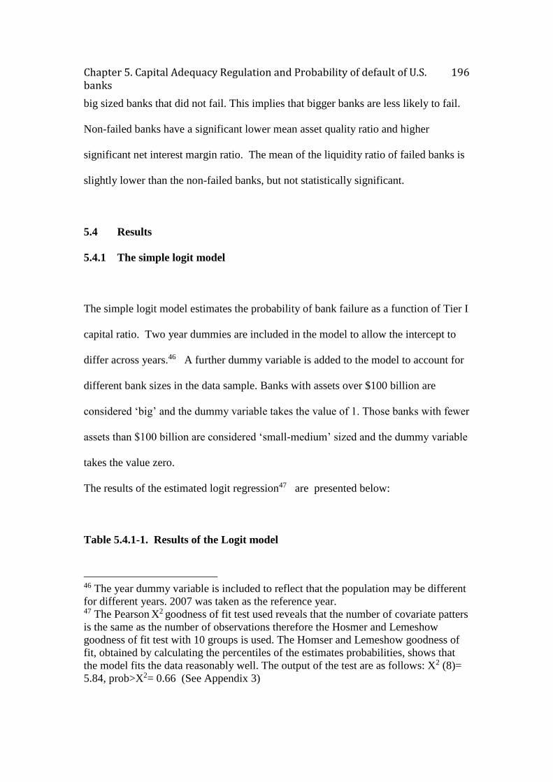
Chapter 5. Capital Adequacy Regulation and Probability of default of U.S. banks
196
big sized banks that did not fail. This implies that bigger banks are less likely to fail.
Non-failed banks have a significant lower mean asset quality ratio and higher
significant net interest margin ratio. The mean of the liquidity ratio of failed banks is
slightly lower than the non-failed banks, but not statistically significant.
5.4 Results
5.4.1 The simple logit model
The simple logit model estimates the probability of bank failure as a function of Tier I
capital ratio. Two year dummies are included in the model to allow the intercept to
differ across years.46 A further dummy variable is added to the model to account for
different bank sizes in the data sample. Banks with assets over $100 billion are
considered ‘big’ and the dummy variable takes the value of 1. Those banks with fewer
assets than $100 billion are considered ‘small-medium’ sized and the dummy variable
takes the value zero.
The results of the estimated logit regression47 are presented below:
Table 5.4.1-1. Results of the Logit model
46 The year dummy variable is included to reflect that the population may be different
for different years. 2007 was taken as the reference year. 47 The Pearson X2 goodness of fit test used reveals that the number of covariate patters
is the same as the number of observations therefore the Hosmer and Lemeshow
goodness of fit test with 10 groups is used. The Homser and Lemeshow goodness of
fit, obtained by calculating the percentiles of the estimates probabilities, shows that
the model fits the data reasonably well. The output of the test are as follows: X2 (8)=
5.84, prob>X2= 0.66 (See Appendix 3)
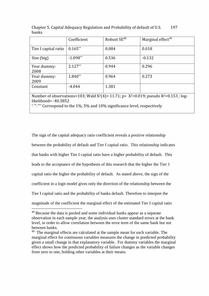
Chapter 5. Capital Adequacy Regulation and Probability of default of U.S. banks
197
Coefficient Robust SE48 Marginal effect49
Tier I capital ratio 0.165** 0.084 0.018
Size (big) -1.098** 0.536 -0.132
Year dummy: 2008
2.127** 0.944 0.296
Year dummy: 2009
1.840** 0.964 0.273
Constant -4.044 1.381
Number of observations=103; Wald Χ2(4)= 11.71; p> Χ2=0.019; pseudo R2=0.153 ; log-likelihood= -40.3852 *, **, *** Correspond to the 1%, 5% and 10% significance level, respectively
The sign of the capital adequacy ratio coefficient reveals a positive relationship
between the probability of default and Tier I capital ratio. This relationship indicates
that banks with higher Tier I capital ratio have a higher probability of default. This
leads to the acceptance of the hypothesis of this research that the higher the Tier 1
capital ratio the higher the probability of default. As stated above, the sign of the
coefficient in a logit model gives only the direction of the relationship between the
Tier I capital ratio and the probability of banks default. Therefore to interpret the
magnitude of the coefficient the marginal effect of the estimated Tier I capital ratio
48 Because the data is pooled and some individual banks appear as a separate
observation in each sample year, the analysis uses cluster standard errors at the bank
level, in order to allow correlation between the error term of the same bank but not
between banks. 49 The marginal effects are calculated at the sample mean for each variable. The
marginal effect for continuous variables measures the change in predicted probability
given a small change in that explanatory variable. For dummy variables the marginal
effect shows how the predicted probability of failure changes as the variable changes
from zero to one, holding other variables at their means.
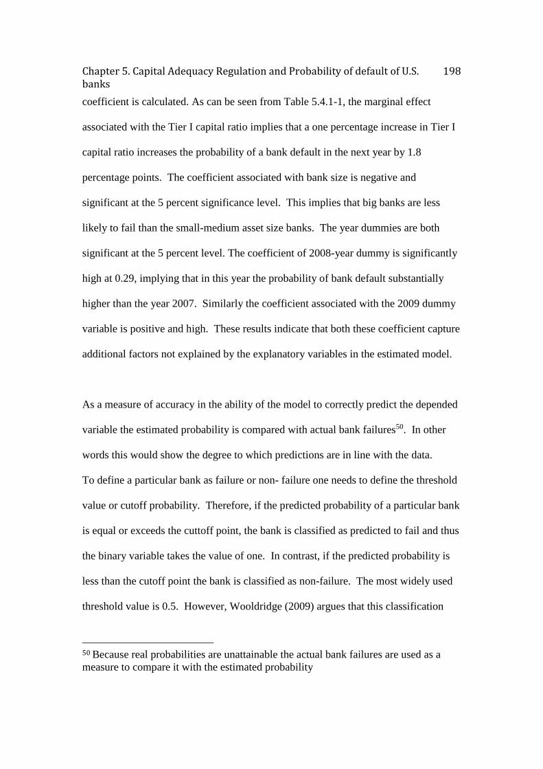
Chapter 5. Capital Adequacy Regulation and Probability of default of U.S. banks
198
coefficient is calculated. As can be seen from Table 5.4.1-1, the marginal effect
associated with the Tier I capital ratio implies that a one percentage increase in Tier I
capital ratio increases the probability of a bank default in the next year by 1.8
percentage points. The coefficient associated with bank size is negative and
significant at the 5 percent significance level. This implies that big banks are less
likely to fail than the small-medium asset size banks. The year dummies are both
significant at the 5 percent level. The coefficient of 2008-year dummy is significantly
high at 0.29, implying that in this year the probability of bank default substantially
higher than the year 2007. Similarly the coefficient associated with the 2009 dummy
variable is positive and high. These results indicate that both these coefficient capture
additional factors not explained by the explanatory variables in the estimated model.
As a measure of accuracy in the ability of the model to correctly predict the depended
variable the estimated probability is compared with actual bank failures50. In other
words this would show the degree to which predictions are in line with the data.
To define a particular bank as failure or non- failure one needs to define the threshold
value or cutoff probability. Therefore, if the predicted probability of a particular bank
is equal or exceeds the cuttoff point, the bank is classified as predicted to fail and thus
the binary variable takes the value of one. In contrast, if the predicted probability is
less than the cutoff point the bank is classified as non-failure. The most widely used
threshold value is 0.5. However, Wooldridge (2009) argues that this classification
50 Because real probabilities are unattainable the actual bank failures are used as a
measure to compare it with the estimated probability
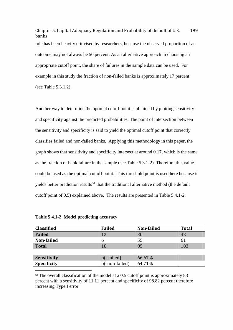
Chapter 5. Capital Adequacy Regulation and Probability of default of U.S. banks
199
rule has been heavily criticised by researchers, because the observed proportion of an
outcome may not always be 50 percent. As an alternative approach in choosing an
appropriate cutoff point, the share of failures in the sample data can be used. For
example in this study the fraction of non-failed banks is approximately 17 percent
(see Table 5.3.1.2).
Another way to determine the optimal cutoff point is obtained by plotting sensitivity
and specificity against the predicted probabilities. The point of intersection between
the sensitivity and specificity is said to yield the optimal cutoff point that correctly
classifies failed and non-failed banks. Applying this methodology in this paper, the
graph shows that sensitivity and specificity intersect at around 0.17, which is the same
as the fraction of bank failure in the sample (see Table 5.3.1-2). Therefore this value
could be used as the optimal cut off point. This threshold point is used here because it
yields better prediction results51 that the traditional alternative method (the default
cutoff point of 0.5) explained above. The results are presented in Table 5.4.1-2.
Table 5.4.1-2 Model predicting accuracy
Classified Failed Non-failed Total
Failed 12 30 42 Non-failed 6 55 61 Total 18 85 103 Sensitivity p(+failed) 66.67% Specificity p(-non-failed) 64.71%
51 The overall classification of the model at a 0.5 cutoff point is approximately 83
percent with a sensitivity of 11.11 percent and specificity of 98.82 percent therefore
increasing Type I error.
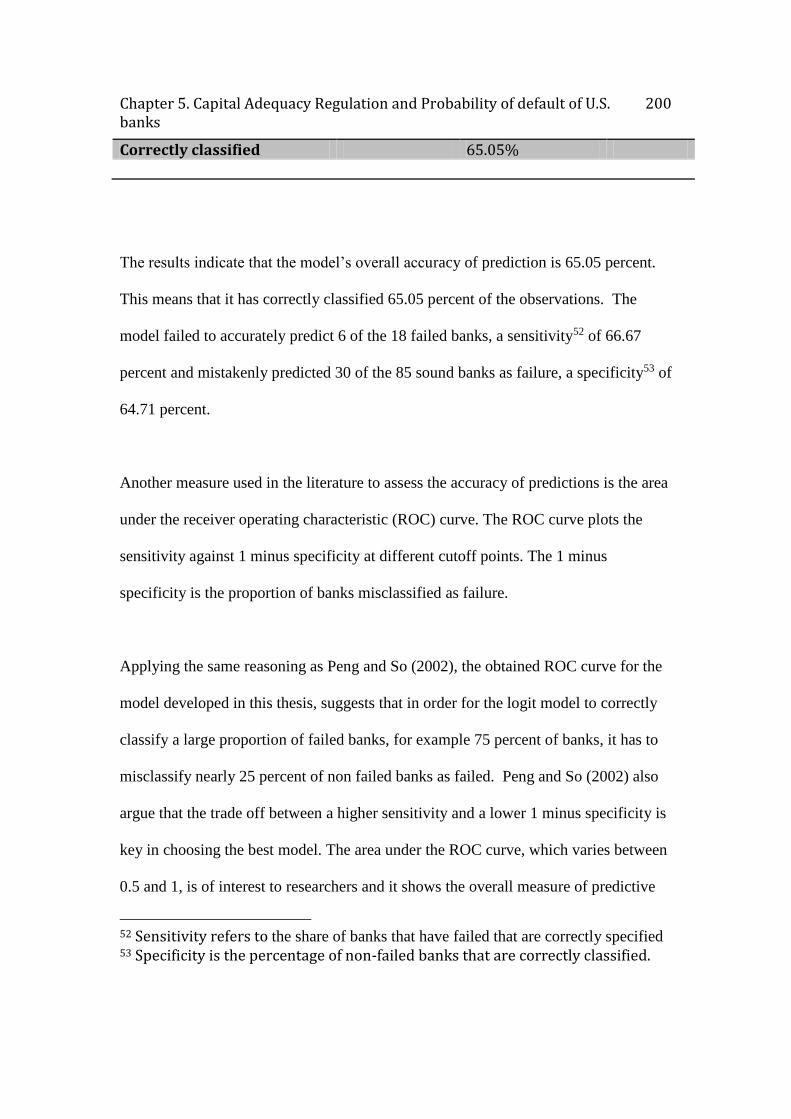
Chapter 5. Capital Adequacy Regulation and Probability of default of U.S. banks
200
Correctly classified 65.05%
The results indicate that the model’s overall accuracy of prediction is 65.05 percent.
This means that it has correctly classified 65.05 percent of the observations. The
model failed to accurately predict 6 of the 18 failed banks, a sensitivity52 of 66.67
percent and mistakenly predicted 30 of the 85 sound banks as failure, a specificity53 of
64.71 percent.
Another measure used in the literature to assess the accuracy of predictions is the area
under the receiver operating characteristic (ROC) curve. The ROC curve plots the
sensitivity against 1 minus specificity at different cutoff points. The 1 minus
specificity is the proportion of banks misclassified as failure.
Applying the same reasoning as Peng and So (2002), the obtained ROC curve for the
model developed in this thesis, suggests that in order for the logit model to correctly
classify a large proportion of failed banks, for example 75 percent of banks, it has to
misclassify nearly 25 percent of non failed banks as failed. Peng and So (2002) also
argue that the trade off between a higher sensitivity and a lower 1 minus specificity is
key in choosing the best model. The area under the ROC curve, which varies between
0.5 and 1, is of interest to researchers and it shows the overall measure of predictive
52 Sensitivity refers to the share of banks that have failed that are correctly specified 53 Specificity is the percentage of non-failed banks that are correctly classified.
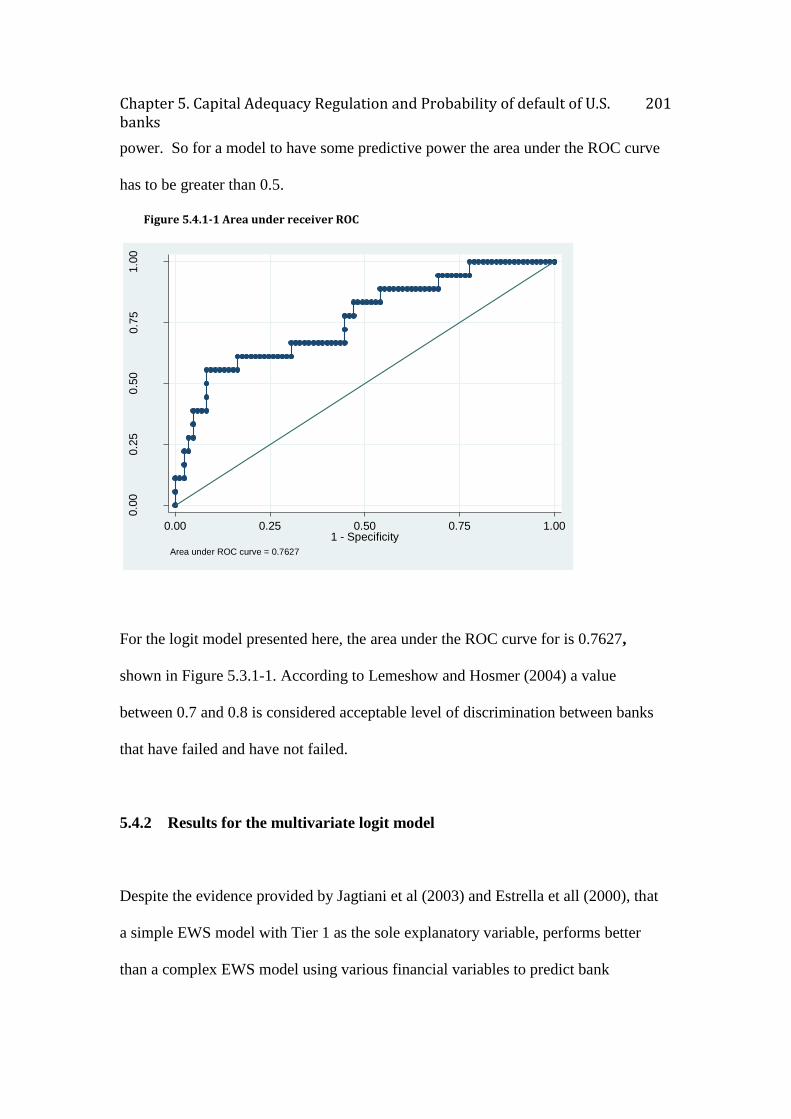
Chapter 5. Capital Adequacy Regulation and Probability of default of U.S. banks
201
power. So for a model to have some predictive power the area under the ROC curve
has to be greater than 0.5.
Figure 5.4.1-1 Area under receiver ROC
For the logit model presented here, the area under the ROC curve for is 0.7627,
shown in Figure 5.3.1-1. According to Lemeshow and Hosmer (2004) a value
between 0.7 and 0.8 is considered acceptable level of discrimination between banks
that have failed and have not failed.
5.4.2 Results for the multivariate logit model
Despite the evidence provided by Jagtiani et al (2003) and Estrella et all (2000), that
a simple EWS model with Tier 1 as the sole explanatory variable, performs better
than a complex EWS model using various financial variables to predict bank
0.0
00.2
50.5
00.7
51.0
0
Sen
sitiv
ity
0.00 0.25 0.50 0.75 1.001 - Specificity
Area under ROC curve = 0.7627
Chapter 5. Capital Adequacy Regulation and Probability of default of U.S. banks
202
probability of default, the latter model is most commonly used by the literature. This
paper estimates both a simple logit model presented above, and a multivariate logit
model, in an attempt to find a model with the highest predictability accuracy. In such
attempt, the analysis here adds three additional financial variables 54to the previous
model. Furthermore the unweighted capital ratio, equity to total assets, is included in
the model.
The net interest margin ratio is used as a proxy for profitability. The relationship
between this ratio and the probability of default is expected to be negative, so the
higher the profitability ratio the lower the probability of bank default. The ratio of
liquid assets to deposits and short-term funding is used as a proxy for liquidity ratio
and it intends to gauge the ability of banks to meet customer deposits and short term
funding in the event of sudden large withdrawals. The higher the ratio of liquid assets
to customer deposits and short term funding the more liquid a bank is supposed to be,
hence the lower the probability of default. As a measure of banks’ asset quality the
net charge-off and average gross loans ratio is used. The ratio intends to measure the
percentage of bad loans that is not recoverable. The lower this ratio is the lower the
probability of banks’ defaults.
The results of the multivariate logit model are presented below:
Table 5.4.2-1 Results of the multivariate logit model
54 The analysis has made use of all the financial ratios available from Bankscope
database.
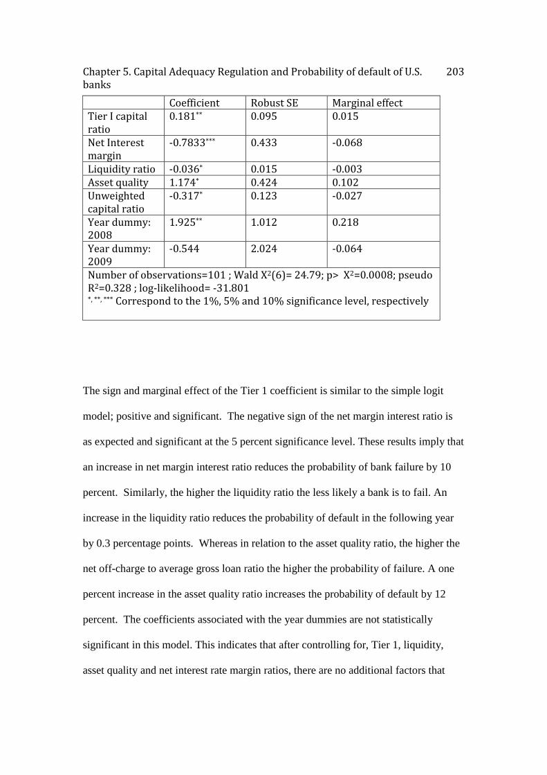
Chapter 5. Capital Adequacy Regulation and Probability of default of U.S. banks
203
The sign and marginal effect of the Tier 1 coefficient is similar to the simple logit
model; positive and significant. The negative sign of the net margin interest ratio is
as expected and significant at the 5 percent significance level. These results imply that
an increase in net margin interest ratio reduces the probability of bank failure by 10
percent. Similarly, the higher the liquidity ratio the less likely a bank is to fail. An
increase in the liquidity ratio reduces the probability of default in the following year
by 0.3 percentage points. Whereas in relation to the asset quality ratio, the higher the
net off-charge to average gross loan ratio the higher the probability of failure. A one
percent increase in the asset quality ratio increases the probability of default by 12
percent. The coefficients associated with the year dummies are not statistically
significant in this model. This indicates that after controlling for, Tier 1, liquidity,
asset quality and net interest rate margin ratios, there are no additional factors that
Coefficient Robust SE Marginal effect Tier I capital ratio
0.181** 0.095 0.015
Net Interest margin
-0.7833*** 0.433 -0.068
Liquidity ratio -0.036* 0.015 -0.003 Asset quality 1.174* 0.424 0.102 Unweighted capital ratio
-0.317* 0.123 -0.027
Year dummy: 2008
1.925** 1.012 0.218
Year dummy: 2009
-0.544 2.024 -0.064
Number of observations=101 ; Wald Χ2(6)= 24.79; p> Χ2=0.0008; pseudo R2=0.328 ; log-likelihood= -31.801 *, **, *** Correspond to the 1%, 5% and 10% significance level, respectively
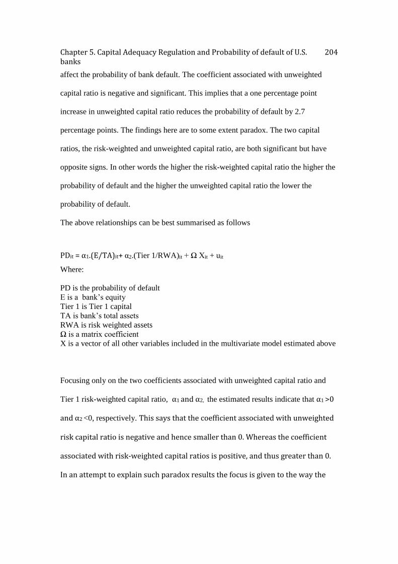
Chapter 5. Capital Adequacy Regulation and Probability of default of U.S. banks
204
affect the probability of bank default. The coefficient associated with unweighted
capital ratio is negative and significant. This implies that a one percentage point
increase in unweighted capital ratio reduces the probability of default by 2.7
percentage points. The findings here are to some extent paradox. The two capital
ratios, the risk-weighted and unweighted capital ratio, are both significant but have
opposite signs. In other words the higher the risk-weighted capital ratio the higher the
probability of default and the higher the unweighted capital ratio the lower the
probability of default.
The above relationships can be best summarised as follows
PDit = α1.(E/TA)it+ α2.(Tier 1/RWA)it + Ω Xit + uit
Where:
PD is the probability of default
E is a bank’s equity
Tier 1 is Tier 1 capital
TA is bank’s total assets
RWA is risk weighted assets
Ω is a matrix coefficient
X is a vector of all other variables included in the multivariate model estimated above
Focusing only on the two coefficients associated with unweighted capital ratio and
Tier 1 risk-weighted capital ratio, α1 and α2, the estimated results indicate that α1 >0
and α2 <0, respectively. This says that the coefficient associated with unweighted
risk capital ratio is negative and hence smaller than 0. Whereas the coefficient
associated with risk-weighted capital ratios is positive, and thus greater than 0.
In an attempt to explain such paradox results the focus is given to the way the
Chapter 5. Capital Adequacy Regulation and Probability of default of U.S. banks
205
two capital ratios are constructed. Assuming the numerators to be the same in
both ratios the denominators are further elaborated. This is because in effect
Tier 1 capital and Equity can be taken to be common to both ratios. However the
denominators are constructed differently. The difference between them consists
in that TA contains all assets at book value and RWA is equal to TA minus risk-
free assets, and a proportion of all other assets proportionate to the estimated
risk in their asset class. A possible explanation is that true risk is in inverse to
estimated risk. This on the other hand suggests that many experts have
estimated risk wrongly and consistently.
A more likely explanation may be found by understanding the market process
that would give rise to such paradox results. The conventional risk-weighting
approach presumes that risk is intrinsic to particular asset categories distinct
probability of default on payment to the bank holding them. Such ‘risky’ assets
therefore have their liquidity permanently reduced (a bank holding them must
set aside capital against the risk that is supposed to be inherent in the assets).
The risk here is the risk of insolvency.
However this ignores the risk of illiquidity in the capital market. The assets that
would be more vulnerable to this kind of risk are more likely to be risk-free
assets, which are traded more commonly in the capital market. They are
therefore more vulnerable to a fall in the liquidity of the capital market. Such a
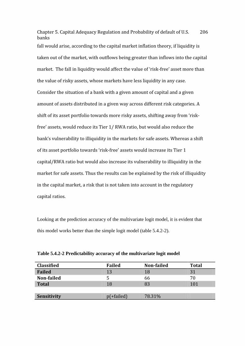
Chapter 5. Capital Adequacy Regulation and Probability of default of U.S. banks
206
fall would arise, according to the capital market inflation theory, if liquidity is
taken out of the market, with outflows being greater than inflows into the capital
market. The fall in liquidity would affect the value of ‘risk-free’ asset more than
the value of risky assets, whose markets have less liquidity in any case.
Consider the situation of a bank with a given amount of capital and a given
amount of assets distributed in a given way across different risk categories. A
shift of its asset portfolio towards more risky assets, shifting away from ‘risk-
free’ assets, would reduce its Tier 1/ RWA ratio, but would also reduce the
bank’s vulnerability to illiquidity in the markets for safe assets. Whereas a shift
of its asset portfolio towards ‘risk-free’ assets would increase its Tier 1
capital/RWA ratio but would also increase its vulnerability to illiquidity in the
market for safe assets. Thus the results can be explained by the risk of illiquidity
in the capital market, a risk that is not taken into account in the regulatory
capital ratios.
Looking at the prediction accuracy of the multivariate logit model, it is evident that
this model works better than the simple logit model (table 5.4.2-2).
Table 5.4.2-2 Predictability accuracy of the multivariate logit model
Classified Failed Non-failed Total
Failed 13 18 31 Non-failed 5 66 70 Total 18 83 101 Sensitivity p(+failed) 78.31%
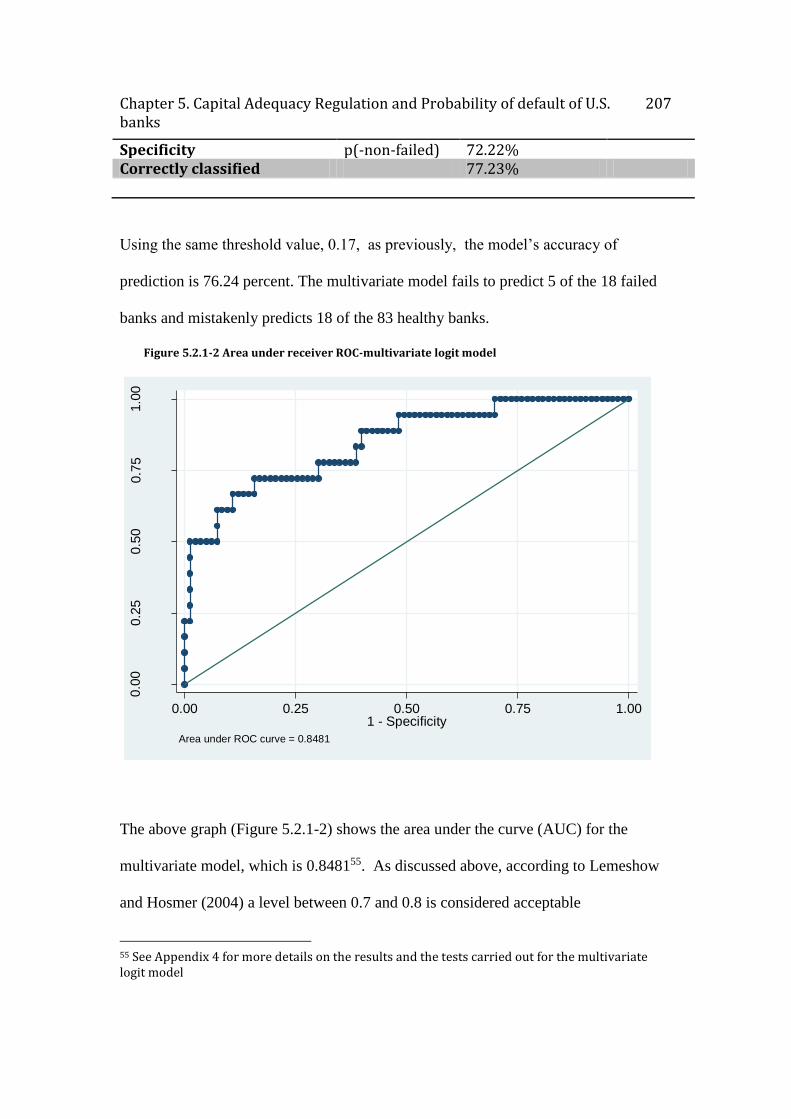
Chapter 5. Capital Adequacy Regulation and Probability of default of U.S. banks
207
Specificity p(-non-failed) 72.22% Correctly classified 77.23%
Using the same threshold value, 0.17, as previously, the model’s accuracy of
prediction is 76.24 percent. The multivariate model fails to predict 5 of the 18 failed
banks and mistakenly predicts 18 of the 83 healthy banks.
Figure 5.2.1-2 Area under receiver ROC-multivariate logit model
The above graph (Figure 5.2.1-2) shows the area under the curve (AUC) for the
multivariate model, which is 0.848155. As discussed above, according to Lemeshow
and Hosmer (2004) a level between 0.7 and 0.8 is considered acceptable
55 See Appendix 4 for more details on the results and the tests carried out for the multivariate logit model
0.0
00.2
50.5
00.7
51.0
0
Sen
sitiv
ity
0.00 0.25 0.50 0.75 1.001 - Specificity
Area under ROC curve = 0.8481
Chapter 5. Capital Adequacy Regulation and Probability of default of U.S. banks
208
discrimination. However, in this case the AUC is slightly higher than 0.8, which
makes it excellent discrimination. This provides evidence that in this analysis the
multivariate logit model works better than the simple model in predicting bank
failure.
5.5 Implications
The empirical results presented in this chapter imply that banks with higher Tier I
capital ratios have a higher probability of default. The use of Tier I capital ratio as the
main predictor of the probability of default was chosen to better capture the effect of
such regulation on the capital markets, and thus on the rest of the economy. Even
though the elements of Tier I capital ratios are mainly shareholder’s equity and
retained earnings, this analysis assumes that banks adjust to higher capital standards
by means of issuing equity. The analysis has also incorporated other financial ratios
as potential factors in determining the probability of defaults. All these variables are
found to have significant power in determining the likelihood of banks’ failure.
However, the main variable of interest to the analysis has been the Tier I capital ratio
which supports the assumptions of this thesis. The results not only validate the
assumptions of the capital market inflation theory, but also implicitly stress the
consequences of these requirements on the rest of the economy, which can be far-
reaching. The point of the argument is that forcing banks to maintain higher risk-
weighted capital ratios not only does not make them safer; on the contrary it increases
their probability of default, crowds out private investment which further damages the
Chapter 5. Capital Adequacy Regulation and Probability of default of U.S. banks
209
economy and concentrates risk in the shadow banking system. Furthermore the
findings of this chapter suggest that the higher the unweighed capital ratios the lower
the probability of default. The implication of such paradox results is that the current
risk-weighted capital requirements only account for risk of insolvency. There is
however a more important risk that needs to be taken into accounts, that of liquidity in
the capital market which explains the negative relationship between the simple
unweighted capital ratios and the probability of banks default.
As explained above, most banks on the verge of collapse can be rescued by
governments. Thus, even though bank failure, in itself, could indeed have major
consequences for the functioning of the economy, governments to some extend lessen
their negative impact by means of providing funds so they continue to operate and
also by providing 100 percent insurance to their depositors. However, inadequate
productive investment in the economy, conducted by non-financial corporations,
proves to be a very hard disease to cure. The low levels of fixed capital formations
have raised concerns over the last few years in the US. Smithers (2014) argues that
US corporations’ debt levels have increased whilst their capital investment remains
very low in proportion to the cash flow. The implications of the reduced levels of
productive investment by US non-financial corporations in the US could be a
contributing factor in the slow recuperating process of a struggling economy. In fact,
the importance and the role of productive investment by corporations have also been
evident in the Japanese economy during the 1990s, that is further examined in the
next chapter.
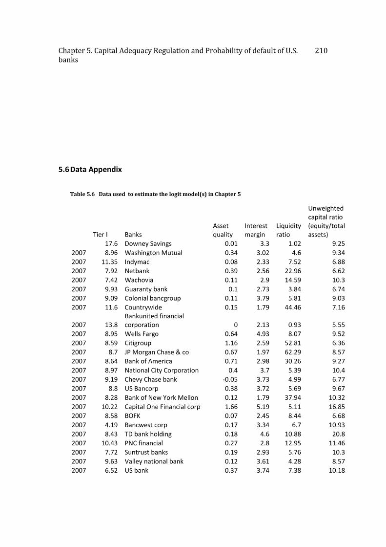
Chapter 5. Capital Adequacy Regulation and Probability of default of U.S. banks
210
5.6 Data Appendix
Table 5.6 Data used to estimate the logit model(s) in Chapter 5
Tier I Banks
Asset quality
Interest margin
Liquidity ratio
Unweighted capital ratio (equity/total assets)
17.6 Downey Savings 0.01 3.3 1.02 9.25
2007 8.96 Washington Mutual 0.34 3.02 4.6 9.34
2007 11.35 Indymac 0.08 2.33 7.52 6.88
2007 7.92 Netbank 0.39 2.56 22.96 6.62
2007 7.42 Wachovia 0.11 2.9 14.59 10.3
2007 9.93 Guaranty bank 0.1 2.73 3.84 6.74
2007 9.09 Colonial bancgroup 0.11 3.79 5.81 9.03
2007 11.6 Countrywide 0.15 1.79 44.46 7.16
2007 13.8 Bankunited financial corporation 0 2.13 0.93 5.55
2007 8.95 Wells Fargo 0.64 4.93 8.07 9.52
2007 8.59 Citigroup 1.16 2.59 52.81 6.36
2007 8.7 JP Morgan Chase & co 0.67 1.97 62.29 8.57
2007 8.64 Bank of America 0.71 2.98 30.26 9.27
2007 8.97 National City Corporation 0.4 3.7 5.39 10.4
2007 9.19 Chevy Chase bank -0.05 3.73 4.99 6.77
2007 8.8 US Bancorp 0.38 3.72 5.69 9.67
2007 8.28 Bank of New York Mellon 0.12 1.79 37.94 10.32
2007 10.22 Capital One Financial corp 1.66 5.19 5.11 16.85
2007 8.58 BOFK 0.07 2.45 8.44 6.68
2007 4.19 Bancwest corp 0.17 3.34 6.7 10.93
2007 8.43 TD bank holding 0.18 4.6 10.88 20.8
2007 10.43 PNC financial 0.27 2.8 12.95 11.46
2007 7.72 Suntrust banks 0.19 2.93 5.76 10.3
2007 9.63 Valley national bank 0.12 3.61 4.28 8.57
2007 6.52 US bank 0.37 3.74 7.38 10.18
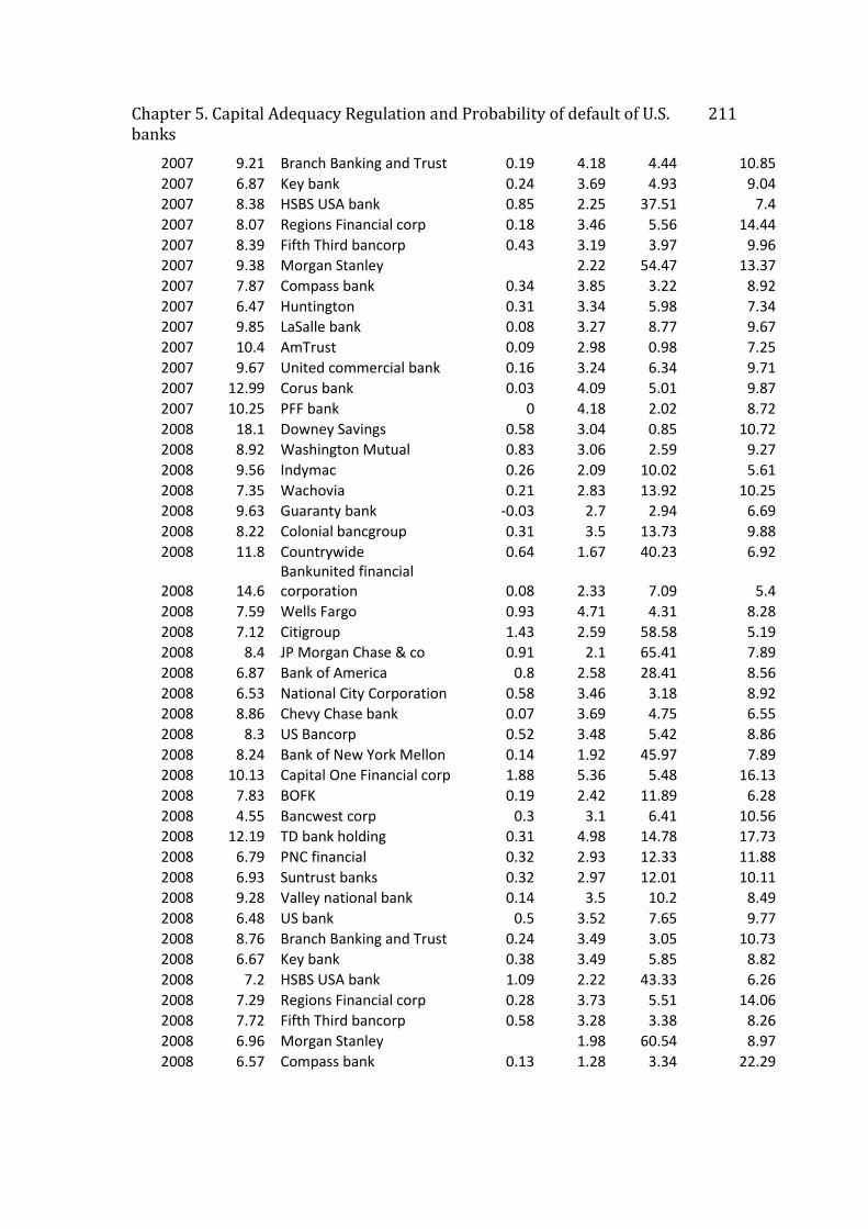
Chapter 5. Capital Adequacy Regulation and Probability of default of U.S. banks
211
2007 9.21 Branch Banking and Trust 0.19 4.18 4.44 10.85
2007 6.87 Key bank 0.24 3.69 4.93 9.04
2007 8.38 HSBS USA bank 0.85 2.25 37.51 7.4
2007 8.07 Regions Financial corp 0.18 3.46 5.56 14.44
2007 8.39 Fifth Third bancorp 0.43 3.19 3.97 9.96
2007 9.38 Morgan Stanley
2.22 54.47 13.37
2007 7.87 Compass bank 0.34 3.85 3.22 8.92
2007 6.47 Huntington 0.31 3.34 5.98 7.34
2007 9.85 LaSalle bank 0.08 3.27 8.77 9.67
2007 10.4 AmTrust 0.09 2.98 0.98 7.25
2007 9.67 United commercial bank 0.16 3.24 6.34 9.71
2007 12.99 Corus bank 0.03 4.09 5.01 9.87
2007 10.25 PFF bank 0 4.18 2.02 8.72
2008 18.1 Downey Savings 0.58 3.04 0.85 10.72
2008 8.92 Washington Mutual 0.83 3.06 2.59 9.27
2008 9.56 Indymac 0.26 2.09 10.02 5.61
2008 7.35 Wachovia 0.21 2.83 13.92 10.25
2008 9.63 Guaranty bank -0.03 2.7 2.94 6.69
2008 8.22 Colonial bancgroup 0.31 3.5 13.73 9.88
2008 11.8 Countrywide 0.64 1.67 40.23 6.92
2008 14.6 Bankunited financial corporation 0.08 2.33 7.09 5.4
2008 7.59 Wells Fargo 0.93 4.71 4.31 8.28
2008 7.12 Citigroup 1.43 2.59 58.58 5.19
2008 8.4 JP Morgan Chase & co 0.91 2.1 65.41 7.89
2008 6.87 Bank of America 0.8 2.58 28.41 8.56
2008 6.53 National City Corporation 0.58 3.46 3.18 8.92
2008 8.86 Chevy Chase bank 0.07 3.69 4.75 6.55
2008 8.3 US Bancorp 0.52 3.48 5.42 8.86
2008 8.24 Bank of New York Mellon 0.14 1.92 45.97 7.89
2008 10.13 Capital One Financial corp 1.88 5.36 5.48 16.13
2008 7.83 BOFK 0.19 2.42 11.89 6.28
2008 4.55 Bancwest corp 0.3 3.1 6.41 10.56
2008 12.19 TD bank holding 0.31 4.98 14.78 17.73
2008 6.79 PNC financial 0.32 2.93 12.33 11.88
2008 6.93 Suntrust banks 0.32 2.97 12.01 10.11
2008 9.28 Valley national bank 0.14 3.5 10.2 8.49
2008 6.48 US bank 0.5 3.52 7.65 9.77
2008 8.76 Branch Banking and Trust 0.24 3.49 3.05 10.73
2008 6.67 Key bank 0.38 3.49 5.85 8.82
2008 7.2 HSBS USA bank 1.09 2.22 43.33 6.26
2008 7.29 Regions Financial corp 0.28 3.73 5.51 14.06
2008 7.72 Fifth Third bancorp 0.58 3.28 3.38 8.26
2008 6.96 Morgan Stanley
1.98 60.54 8.97
2008 6.57 Compass bank 0.13 1.28 3.34 22.29
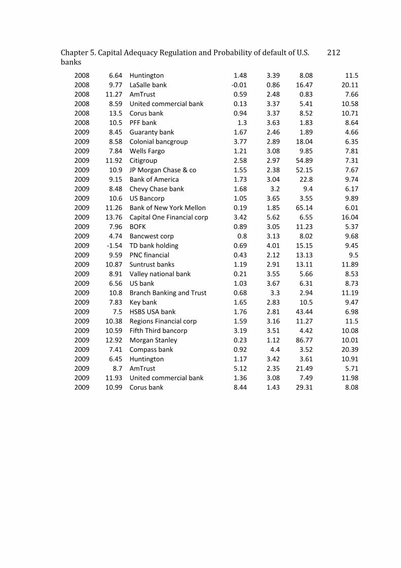
Chapter 5. Capital Adequacy Regulation and Probability of default of U.S. banks
212
2008 6.64 Huntington 1.48 3.39 8.08 11.5
2008 9.77 LaSalle bank -0.01 0.86 16.47 20.11
2008 11.27 AmTrust 0.59 2.48 0.83 7.66
2008 8.59 United commercial bank 0.13 3.37 5.41 10.58
2008 13.5 Corus bank 0.94 3.37 8.52 10.71
2008 10.5 PFF bank 1.3 3.63 1.83 8.64
2009 8.45 Guaranty bank 1.67 2.46 1.89 4.66
2009 8.58 Colonial bancgroup 3.77 2.89 18.04 6.35
2009 7.84 Wells Fargo 1.21 3.08 9.85 7.81
2009 11.92 Citigroup 2.58 2.97 54.89 7.31
2009 10.9 JP Morgan Chase & co 1.55 2.38 52.15 7.67
2009 9.15 Bank of America 1.73 3.04 22.8 9.74
2009 8.48 Chevy Chase bank 1.68 3.2 9.4 6.17
2009 10.6 US Bancorp 1.05 3.65 3.55 9.89
2009 11.26 Bank of New York Mellon 0.19 1.85 65.14 6.01
2009 13.76 Capital One Financial corp 3.42 5.62 6.55 16.04
2009 7.96 BOFK 0.89 3.05 11.23 5.37
2009 4.74 Bancwest corp 0.8 3.13 8.02 9.68
2009 -1.54 TD bank holding 0.69 4.01 15.15 9.45
2009 9.59 PNC financial 0.43 2.12 13.13 9.5
2009 10.87 Suntrust banks 1.19 2.91 13.11 11.89
2009 8.91 Valley national bank 0.21 3.55 5.66 8.53
2009 6.56 US bank 1.03 3.67 6.31 8.73
2009 10.8 Branch Banking and Trust 0.68 3.3 2.94 11.19
2009 7.83 Key bank 1.65 2.83 10.5 9.47
2009 7.5 HSBS USA bank 1.76 2.81 43.44 6.98
2009 10.38 Regions Financial corp 1.59 3.16 11.27 11.5
2009 10.59 Fifth Third bancorp 3.19 3.51 4.42 10.08
2009 12.92 Morgan Stanley 0.23 1.12 86.77 10.01
2009 7.41 Compass bank 0.92 4.4 3.52 20.39
2009 6.45 Huntington 1.17 3.42 3.61 10.91
2009 8.7 AmTrust 5.12 2.35 21.49 5.71
2009 11.93 United commercial bank 1.36 3.08 7.49 11.98
2009 10.99 Corus bank 8.44 1.43 29.31 8.08
213
Chapter 6. The Probability of Bank Default – The Case of
Japan
This chapter provides empirical evidence on the impact of capital adequacy regulation
on the probabilities of default of Japanese banks, using the same methodology as in
chapter 5. However, contrary to the time period chosen for the US banking sector, that
of 2007-2009 which is associated with Basel II Accord, for Japan the period between
1998-2000, during which Basel I capital requirements were in place, is chosen to
empirically evaluate such impact on the Japanese banking sector. This time period is
chosen to reflect the large number of bank failures associated with the Japanese
banking sector at the time, discussed in detail in section 6.2 of this chapter. Section
6.3 discusses the empirical results which, as in the case of US, indicate that banks
with a higher Tier I capital ratios have a higher probability of default. Section 6.4
concludes.
6.1 Probability of bank default- the case of Japan
The 2007-2008 US banking crisis serves as a warning that such a crisis can be
inevitable even for a (perceived) healthy and sophisticated financial system. The
Chapter 6. The Probability of Bank Default – The Case of Japan 214
1990s Japanese banking crisis and its aftermath, however, serves as a lesson that the
costs of having such crises can be so considerable as to cause the economy to remain
stagnant for years, as in the case of Japan. Prior to the bubble burst, the Japanese
economy was characterised by a period of high economic growth, dubbed ‘miracle’
economic growth in the period from mid 1953 to early 1973. After the occupation
period ended, Japan’s economy growth rate was at the average with the rest of the
world, but it soon became one of the highest growth economies, averaging 10 percent
growth per year. During the early 1970s its growth rated slowed, to an average of 4
percent per annum, but was still considered the highest amongst other advanced
economies. In the late 1980s Japanese banks were considered to be among the
strongest in the world. In 1988, seven Japanese banks were ranked among the world’s
top ten largest banks by assets (Hoshi 2001). However, in the aftermath of its stock
market crash in 1989, the Japanese economy entered a prolong slump from which it
has yet to fully recover. The slowdown in economic growth and the onset of asset
price deflation had a significant negative impact on the health of Japanese banks and
other financial institutions. In the years that followed the stock market crash, the
soundness of the Japanese banking system weakened, culminating in 1997 with the
spectacular failures of several highly important financial institutions. The large
number of banks failures occurred despite the then newly introduced Basel I capital
requirements. As explained earlier, Basel I was introduced in 1988 and was fully
implemented in Japan in March 199356.
56 The end of fiscal year 1992, in Japan
Chapter 6. The Probability of Bank Default – The Case of Japan 215
Judging just on the number of bank failures the country experienced during the 1990s
and early 2000s one can easily reject the notion of the Basel capital requirements
aiming to make banks more secure. Furthermore the research in this thesis provides
empirical evidence that does not support the capital regulatory standards, arguing that
under conditions of capital market deflation requiring banks to hold higher capital
ratios makes them more prone to failure.
After more than a decade of repeated failures and poor performances Japanese banks
now not only seem to have recovered but also are trying regain their position at the
international level. The Economist in 2011 published an article about Japanese
banks, titled ‘Back from the dead’, where it is argued that not only the country’s three
main banks are amongst top 30 largest banks in the world, by assets, but also how
these banks used the crisis in their favour by expanding internationally in countries
such US, Europe and Asia (see below)(The Economist 2011a). Nevertheless, in terms
of economic (growth) performance Japan still has yet to recover fully. Following a
slight expansion in mid 2000s, the global financial crisis and the Tahoku Earthquake
and Tsunami of 2011 brought yet more obstacles in achieving sustainable growth.
Lipscy and Takinami (2013), note that in nominal terms Japan’s GDP has remained
the same in two decades. In 1991 Japanese nominal GDP was recorded to have been
470 trillion yen and in 2012 this figure was nearly the same totalling 471 trillion yen.
This chapter makes use of the same empirical and methodology framework as the
previous one. Using the capital market inflation theory the probability of bank default
Chapter 6. The Probability of Bank Default – The Case of Japan 216
is estimated using Tier I capital ratio as the sole predictor. A simple logit model is
estimated on a pool cross sectional data for the period 1998-2000.
As discussed in chapter 3, even though this thesis find no explicit evidence of the
capital market inflation since 1990, the empirical predictions on the relationship
between Japan’s central bank stock purchases and Nikkei stock price movement
indicate that the capital market inflation still holds. Furthermore, the arguments
presented below and elsewhere in the literature are sufficient to conclude that
inflation has been a phenomenon in the country’s capital market prior to the period
under consideration57.
Analysing the Japanese banks probability of default during the 1990s financial crisis
is perhaps more revealing than the case of US or any other country. That is mainly for
two reasons. The first reason is the timing of both the financial crisis and the
introduction of capital requirements that occurred during the 1990s. In the aftermath
of the financial crisis, banks were under major pressure to meet the regulatory capital
standards in deteriorating market conditions. As argued below, the introduction of the
Basel capital requirements had a huge negative impact on Japanese banks. For
example, Peek and Rosengren (1999) argue that most international active Japanese
banks, such as Daiwa, Yasuda Trust, Mitsui Trust and Nippon Credit Bank, in the
1990s announced plans to close their overseas operations as a consequence of the
57 And during banks capital adjustment process in meeting the Basel regulatory
standards which began in 1988.
Chapter 6. The Probability of Bank Default – The Case of Japan 217
difficulties they faced to comply with the international capital requirements.
Operating only as domestic banks allowed them to hold lower capital ratios. One
interesting fact about these banks is that, following their decision to close
international operations, all of them either failed, or were rescued by the government,
or were forced to merge with another bank (as explained below). Shimizu (2007), on
the other hand argues that the Basel regulatory framework failed to take into account
the conditions of the Japanese financial market. He states that ‘when, however, some
macro shocks emerged for which individual banks has no control, the BIS regulation
should aggravate the macro economic conditions of the BIS criteria did not adjusted
somehow. This is a lesson we can learn from Japan’s experience in the 1990s’
(Shimizu 2007, pg. 4)
These facts provide a foundation in building an argument that identifies the timing of
these regulatory standards as a possible added factor in exacerbating the problems in
the Japanese banking sector.
The second reason is linked to the capital market inflation theory this thesis employs
to explain probability of bank default. The underlying assumptions of this theory are
closely associated with the evidence that the crisis has brought about. Not only did the
country experienced a prolonged recession that lasted over 15 years, but also the
productive investment of the Japanese corporations steadily declined during this
period. As argued above, the Basel capital requirements were implemented at a time
when the capital market conditions were weak, in the aftermath of the stock market
Chapter 6. The Probability of Bank Default – The Case of Japan 218
crash in 1990. Therefore banks had to offer a higher price in order to raise their
needed regulatory capital. There is mounting evidence in the literature that records
the substantial reduction in the productive investment by Japanese corporations
during the 1990s. These facts support the underlying assumptions of the capital
market inflation theory, that forcing banks to hold higher capital ratios is a way of
crowding-out the nonfinancial sector, which may lead to a decline in fixed capital
formation. Banks inelastic demand for capital at the time could have indeed been a
factor contributing to the reduction of productive investment by Japanese corporations
during the crisis. If banks would have not been under major demand to meet such
regulatory capital ratios, the capital market might have been an (alternative)
important source of funding that would have assisted the Japanese firms not only to
overcome the difficulties they faced in the aftermath of the crisis but also to fund
future productive investment.
6.2 The Japanese banking system
Given the vast amount of literature devoted to Japan it is perhaps safe to claim that its
economy is one of the most studied economies of all times. This is both in explaining
the high economic growth the country experienced during the period 1953-1973, and
the prolonged recession the country experienced during the 1990s and the subsequent
slow recovery. During the boom decades the Japanese annual average real economic
growth was around 10 percent, making Japan the world’s second largest economy,
after the US (Ohno 2006). Over the same period Japan also became the world’s
Chapter 6. The Probability of Bank Default – The Case of Japan 219
leading exporter of steel and automobiles (Krugman 2009). However, the high
economic growth era ended after 1973, when growth rates fell to around 4 percent.
Barsky (2009) states that the economy started to shows signs of recovery, in 1986,
when figures of GDP, corporate earning and dividends started to increase. Many mark
this period as the start of the ‘bubble economy’ and associate it with the Plaza
Accord in 1985. The agreement reached between the G5 nations, called for a
depreciation of the US dollar against the yen58. As a result, the yen appreciated
substantially, increasing by nearly 46 percent against the dollar. This damaged
Japanese exports, and subsequently the economy. The Japanese government
undertook different policy measures to stimulate the economy. Interest rates were
reduced by approximately 3 percentage points59, followed by the introduction of a
large fiscal package in 1987. By the time of the fiscal stimulus the Japanese economy
had already started to recover, as stated above the economy started to grow again in
1986. The boom was associated with growing credit and rising asset prices. An
exceptionally large increase occurred in stock and land prices, which tripled form
1985 to 1989 (IMF 2011). Indeed prices were so high that the land surrounding the
Imperial Palace in Tokyo was reported to be worth more than the whole state of
California (Krugman 2009). However, in the summer of 1990 the bubble burst and the
stock market crashed.
58 The agreement aimed to devalue the dollar against the deutsche mark as well, given
that Germany and Japan were the two countries with a current account surplus 59 And kept within this range until 1989
Chapter 6. The Probability of Bank Default – The Case of Japan 220
Krawczyk (2006), argues that the privatization programmes undertaken during the
1980s, such as the privatisation of Japan Railway and Nippon Telephone and
Telegraph, together with the partial financial liberalization contributed greatly to the
asset bubble that characterised the Japanese economy at the time.
In the financial markets liberalisation started in the 1970s. Before that the Japanese
financial system was bank based, known as the ‘main bank system’. Corporate firms
had limited access to bond markets and equity issuance was rather minimal (Hoshi
and Kashyap 1999). Therefore, banks were the main external source of finance for
Japanese corporations. With the dissolution of the Keirestu in the 1990s, Japanese
corporations were left with large debts that they could not refinance into equity.
In late 1970s a secondary market for government bonds was created marking the start
of deregulation. This gave investors an alternative investment opportunity to, for
example, bank deposits, which offered rather low interest rates. Financial institutions
at the time in Japan were subject to interest rates controls, which were set in 1947
under the Temporary Interest Rate Adjustment Law (TIRAL). The law permitted the
Bank of Japan (BOJ) to place ceilings on all kinds of deposits rates and on short term
lending rates. All financial institutions, apart from the government financial
institutions and postal savings, were subject to these restrictions. Whereas, shinkin
banks60, agricultural cooperative and the credit cooperatives were not subject to
60 Shinkin banks are non-profit cooperatives known also as credit associations. They
are relatively small in size and are owned by members living in the same geographical
area as the institutions’ headquarters or branches. They operate in the same way as
commercial banks but restrict their lending mostly to members. They could however
locate up 20 percent of their loans to non-members (Hutchison and Westermann
2006).

Chapter 6. The Probability of Bank Default – The Case of Japan 221
lending rates regulation. The introduction of certificates of deposits (CD) in 1979, for
which TIRAL regulation did not apply, marked the start of the deregulation of interest
rates. The restrictions were gradually lifted for all other deposits in stages and in 1994
they were completely abolished (Kanaya and Woo 2000).
The liberalisation of domestic corporate bond and equity markets also started in mid
1970s. Also, the lifting of the foreign exchange controls in 1980 and the abolition of
the ‘real demand principle’ in 1984, allowed firms to obtain finance abroad. Another
step towards financial liberalization was the opening of the Tokyo offshore banking
market in December 1986. These developments created new ways, by which firms
could raise funds, thus reducing their reliance on bank borrowing. Hoshi (2001)
shows that the ratio of bank loans to total assets of large manufacturing firms in the
1970s was nearly 0.35 but declined steadily thereafter, falling to 0.15 in 1990.
In the mean time, banks deregulation was a slower process, and in many respects they
were still subject to tight regulation during the 1980s. For example, banks could not
engage in loan securitization and fee-generating activities until late 1990’s (Hoshi and
Kashyap 1999). Furthermore, the banking industry was still subject to the Securities
and Exchange Act of 194761, which separated investment and commercial banking
activities. With this regulation in place, the role of banks was limited to the traditional
approach, in which deposits are used to make loans. However, when banks lost their
best borrowers to capital markets, they engaged in high- risk lending activities such as
real estate, small and medium businesses, private equity etc.
61 Similar to the US 1933 Glass- Steagall Act.
Chapter 6. The Probability of Bank Default – The Case of Japan 222
When the bubble burst, banks were highly exposed to land, through its use as
collateral but also by lending to jusen companies (see below). As a consequence, the
quality of banks loans deteriorated substantially in the aftermath of the bursting of the
land price bubble. In 1998 the non-performing loans of Japanese banks were
equivalent to 7 percent of GDP (Hoshi and Kashyap 1999).
Japanese banks were only able to be more competitive and engage in non-traditional
operations when the ‘Financial Big Bang’ was were first introduced in 1996 and fully
implemented in 2001. The Big Bang reforms aimed to make the Japanese financial
sector “ free, fair and global”. The programme lifted any restrictions that were in
place between banks, securities industry and insurance sector (Montgomery and
Takahashi 2011).
Thus the stock market crash and the collapse of land prices placed Japanese banks
under considerable financial stress. Kanaya and Woo (2000) provide the following
link of the events that led to the deterioration of the health of the banking system:
Firstly the significant decline in land prices reduced the quality of real estate loans;
secondly, the value of collateral was wiped out; thirdly the lost value of banks’ equity
holdings undermined bank capital and fourthly, debtors were unable to meet their loan
obligations due to weaker economic conditions (Kanaya and Woo 2000, pg. 8).
Chapter 6. The Probability of Bank Default – The Case of Japan 223
The Japanese banking sector started to show signs of weakness in late 1994 when the
operations of two credit cooperatives, Tokyo Kyowa and Anzen Credit were closed.
Tokyo Kyodo Bank was created, funded by the Bank of Japan, commercial banks and
credit cooperatives, by the regulatory bodies to assume all assets and liabilities of the
two insolvent credit cooperatives (Kanaya and Woo 2000). A year later two credit
unions, the Cosmo Credit Corporation and Kizu Credit Cooperative, and one region
bank, also collapsed. These failures were followed by a scandal over Daiwa bank
later in November that year. The bank was forced to close its operations in the US
following accusations of illegal activities in covering-up around $1.1 trillion in bond
trade losses (Truell 1995).
During the same period Japan experienced the so-called jusen crisis. The jusen
companies, which were specialised housing loan companies, were created in the
1970s by banks and other financial institutions to provide mortgage loans. As non-
deposit taking financial institutions the jusen companies, unlike commercial banks,
were not subject to tight interest rate restriction. During late 1980s and early 1990s
they provided loans in the real estate market (Krawczyk 2006). They were mainly
funded by agricultural cooperatives, which even though they were regulated by the
MOF, were not restricted to lend in the real estate sector (Kanaya and Woo 2000).
When the real estate market started to decline substantially in early 1990’s the quality
of the lending of jusen companies by 1992 became a serious concern. In mid 1995,
after a special evaluation of the jusen companies conducted by the MOF which found
that over 74 percent of their loans were nonrecoverable, seven out of eight jusen
Chapter 6. The Probability of Bank Default – The Case of Japan 224
companies were dissolved (ibid). In order to prevent a panic, which could have led to
massive withdrawals from other financial institutions, which had provided finance to
jusen companies, the Japanese authorities designed a plan to use public funds to
facilitate the liquidation of the seven jusen companies. A special account was
established in the Deposit Insurance Corporation (DIC) to assist such liquidations,
which included nearly 680 billion yen in government funds (GAO 1996). These funds
covered around 10 percent of the losses. While, the parent banks covered the largest
percentage of the losses, some 55 percent, worth 5.3 trillion yen, 27 percent of the
losses was covered by other creditor banks and only 8 percent by the agricultural
cooperatives (Krawczyk 2006).
The jusen crisis together with the failure of the above mentioned financial institutions
led to the so –called ‘Japan Premium’- a premium on borrowing costs of Japanese
banks on international financial markets. Spiegel (2001) relates the premium to
government policy. He states that the failure of Hyogo Bank, the first listed bank
failure in Japan, with assets worth $37 billion, influenced the ‘Japan Premium’. This
is because prior to Hyogo collapse, the Japanese government intervened when needed
to prevent any possible financial institution failure, by arranging a merger of the
insolvent bank with a sound bank62. Within such a policy framework the market
perceived Japanese banks to be solvent and quite safe. However, when the authorities
62 For example, in 1992, Toho Sogo Bank, a small local banks, became insolvent and
the Deposit Insurance Corporation assisted its’ merger with Iyo Bank.
Chapter 6. The Probability of Bank Default – The Case of Japan 225
failed to save Hyogo Bank this perception changed and Japanese banks had to face a
premium on their borrowing costs (Spiegel 2001).
In 1996 some Japanese banks were downgraded by credit rating agencies. The
reduction in credit rating had started since 1989, however in 1996 the reduction was
quite radical. For example for some banks, such as Long Term Credit Bank of Japan,
Nippon Credit Bank, Hokkaido Takushoku Bank and Daiwa, credit ratings were
reduced from A to BBB (Miyajima and Yafeh 2003).
In 1997, the Japanese economy experienced another recession when higher
consumption taxes were implemented. In April 1997, the operations of Nissan Life
Insurance were suspended by the MOF. On 3 November that year Sanyo Securities, a
second-tier securities firm in Japan, filed for bankruptcy, under the Corporate
Rehabilitation Law. On the same day, Sanyo also defaulted on overnight interbank
loans market. This was the first default in the Japanese interbank market. By mid
November, Yamaichi Securities, one of Japan’s large four securities companies, and
Hokkaido Takushoku Bank, one of the country’s city banks, collapsed. On the 26
November, the failure of Tokuyo City bank, a small regional bank, was announced
(Montgomery and Shimizutani 2009). These failures were associated with massive
disruptions in the interbank market, a sell-off of bank shares in the Tokyo Stock
Exchange and an increase in the ‘Japan Premium’ (Kanaya and Woo 2000; Krawczyk
2006).

Chapter 6. The Probability of Bank Default – The Case of Japan 226
Prior to these events Japanese depositors were guaranteed up to 10 billion yen
(approximately $100,000) per account. However, this changed on 26 November 1997,
when then the Minister of Finance announced that the Japanese government would
guarantee 100 percent of the deposits until March 2001. In February 1998, the
Japanese government passed two laws for financial stabilization, allowing the DIC to
use 30 trillion yen of public money to bail out troubled banks and to strengthen
depositor protection. 17 trillion yen was made available to provide full deposit
protection, and the remaining 13 trillion yen went to banks with financial difficulties
(Montgomery and Shimizutani 2009).
In March 1998, 21 banks applied for government funds, with the exception of Tokyo-
Mitsubishi bank that was persuaded to apply for a capital injection. All major city
banks received on average 100 million yen each, whereas three Regional banks,
Yokohoma Bank, Ashikaga Bank and Hokuriku Bank applied for smaller funds (ibid).
In total, 1.8 trillion yen was spent on capital injections, mainly in the form of
subordinated debt, for the banking system.
However financial stabilisation was far from achieved as the crisis continued further
in 1998. In June 1998, the newly created financial regulatory, Financial Supervisory
Agency (FSA), took over supervisory powers from the Ministry of Finance (MOF)
and other regulatory bodies to supervise banks and other financial institutions, such as
Chapter 6. The Probability of Bank Default – The Case of Japan 227
securities firms, insurance companies, shinkin banks and credit cooperatives63. In
October 1998, the Diet passed two laws: the Financial Revitalization and Financial
Early Strengthening Law in an attempt to resolve the problems in the banking system.
Under these laws authorities were able to better deal with bank failures, rather than
just focusing on finding suitable healthy banks to take over failed banks, as well as
having more funds at their disposal for bank resolution. A total of 60 trillion yen (12
percent of GDP) of government funds became available to strengthen the Japanese
banking sector. Out of the 60 trillion yen, 25 trillion yen was allocated to recapitalize
weak but solvent banks, 18 trillion yen for the insolvent banks, to assist their
liquidation and/or nationalisation and 17 trillion yen to fully protect the deposits of
insolvent banks (Kanaya and Woo 2000).
Following the new legislation, in October 1998 the Long Term Credit Bank of Japan
(LTCB) was nationalised. In 1989 LTCB was the ranked the 9th largest bank in the
world by assets, applied voluntarily for nationalisation after suffering massive losses
as a result of the non-performing loans accumulated by lending to the real estate
sector and jusen companies. In March 2000, the bank was sold to the US investment
fund, Ripplewood Holdings, and reopened for business as a private commercial bank,
under the name Shinsei Bank. In November 1998, another nationalisation took place,
that of Nippon Credit Bank. The credit bank was involuntarily nationalised, since
63 MOF had previously supervised banks, securities firms, insurance companies and
other non-bank financial institutions, whereas the Regional Financial Bureaus had
been the supervisor of shinkin banks, and credit cooperative were under the
supervision of prefectural governments (Kanaya and Woo 2000).
Chapter 6. The Probability of Bank Default – The Case of Japan 228
previous attempts to strengthen its financial position were not successful. The bank
was reported to have had a capital deficit of 94 billion yen as of March 1998 (Harada,
Ito and Takahashi 2013). Nippon Credit Bank was later sold and renamed Aozora
Bank in 2001.
In 1999, a second round of capital injection of around 15 trillion yen was provided to
a total of 15 banks. However, this time rather than a standard capital amount, banks
received government funds in accordance to their individual financial needs. In order
to qualify for the requested capital injection, the Financial Revitalization Commission
(FRC), which was established under the Financial Revitalization Law, required banks
to provide a restructuring plan, which had to include plans to raise capital in the
private sector (Montgomery and Shimizutani 2009).
The year 1999 marks the beginning of the so-called ‘merger-wave’ period. In May
that year, Mitsui Trust and Chuo Trust announced their merger plans (Kanaya and
Woo 2000). A few months later, Industrial Bank of Japan, Dai-Ichi Kangyo Bank and
Fuji Bank revealed their merger plans, forming Mizuho Group. All three banks were
amongst the largest banks in Japan, with total assets worth, 42.09 trillion yen, 52.53
trillion yen and 46.38 trillion yen, respectively (Harada and Ito 2012). In October of
the same year Sumitomo Bank and Sakura bank, which had 51.53 trillion yen and
48.30 trillion yen in assets, respectively, also announced that the two banks were to
merge to form Sumitomo Mitsui Financial Group (ibid).
Chapter 6. The Probability of Bank Default – The Case of Japan 229
In March 2000 Asahi Bank, Tokai Bank and Sanwa Bank announced their plan to
merge, forming UFJ Holdings64. At the time of the announcement, Sanwa Bank had
47.59 trillion yen in assets and Tokai Bank’s assets were worth 30.36 trillion yen
(ibid). In April, the creation of the Mitsubishi Tokyo Financial Group was announced.
The group was formed by the merger of Bank of Tokyo-Mitsubishi, which had a total
of 69.81 trillion yen in assets, Mitsubishi Trust Bank, a rather smaller bank with 16.37
trillion yen in asset, and Nippon Trust Bank. In 2001 Daiwa bank and Asahi bank
merged to form Resona Holdings.
Kawai (2003) suggests that the reason behind the ‘merger wave’ period in which large
Japanese banks decided to merge with one another, was financial distress. Merging
was seen not only as a way of becoming more efficient but also, and most
importantly, to avoid failure. Harada and Ito (2008) use the Distance to Default
approach to evaluate the merger effect in the Japanese banking sector for the period
between 1985 and August 2005. They examined four merger cases: that of Mizuho
GF, UFJ Holdings, Sumitomo Mitsui Financial Group and Mitsubishi Tokyo
Financial Group, in order to determine whether a merger bank financially improved,
worsened or remain on average, in comparison with predecessor banks. The evidence
show that merged banks did not necessarily become better off, in the sense that
merging did not ameliorate their financial health (Harada and Ito 2008).
64 Even though Asahi Bank did not join the formation of UFJ Holdings.
Chapter 6. The Probability of Bank Default – The Case of Japan 230
By late 1999, the Japanese banking system took a turn towards stability. Between
1999-2002 there is no recorded major bank failure. This was achieved not only the
capital injection provided by the government but also following the new guidelines of
the newly created FSA to restructure the banking sector. The restructuring was
conducted using different measures such as reducing the number of bank branches
and overseas operations, tighter loan classification65, better provisioning and write-
offs66 and others (Kawai 2003).
However, 2003 proved to be another difficult year for the Japanese banking sector.
The newly created, 5th largest bank in 2003, Resona Bank came under considerable
stress after suffering a massive capital shortage. Resona Holdings capital adequacy
ratio was reported to have been well below 4 percent. In May 2003, As a result the
government injected 1.96 trillion yen of public funds through its subsidiary Resona
Bank. This was followed by the nationalisation of Ashikaga Bank in November of the
same year.
65 Banks in Japan had been able to have a tax-deductible general reserve accounts for
any potential loan losses since 1964. The accounts allowed the classification of
‘normal’ and ‘substandard’ loans, for which any additional specific provision against
the latter classification did not apply. On the other hand banks were required to make
specific provisions not only for loss loans but also for those loans that were doubtful,
out of which 50 percent were tax deductible. 66 Japanese banks were known to have been slow at writing off loans with low
chances of recovery. One reason for this is due to tax rules, which only allowed banks
to write-off loans after losses accruing to those loans had been ascertained in
bankruptcy. Another possible reason was the worry of sending wrong signals to their
customers.
Chapter 6. The Probability of Bank Default – The Case of Japan 231
After more than a decade of repeated failures, insolvency and financial weakness the
Japanese financial system started to gain strength. The economy also started to pick
up around 2003, with GDP growing more than 2 percent and the rate of
unemployment declined (Krugman 2009). The Japanese banking sector, has also now
recovered and in the 2007-08 US crisis looked in much a better position than that of
US. The situation changed in favour of Japan’s banks, which were once heavily
criticised for their structure and took much of the blame for the economic stagnation
the country experienced. Most of the criticism came from commentators in western
developed countries, urging the Japanese authorities to change the regulatory
framework and promote inventiveness (Montgomery and Takahashi 2011). As
explained above, the Japanese banking sector has been heavily regulated and even
after the Big Bang deregulation reforms were implemented its banking sector
remained traditional, in the sense that financial innovation never really took off. In
contrast the US banking sector, with a free market regime, came to be too complex for
its own good, as reflected in the 2007-08 financial crisis. However, during this crisis it
was the US banks that faced major difficulties, and for some it was the Japanese
banks that came to the rescue. For example, in January 2008 Mizuho Financial Group
invested $1.2 billion in purchasing 18 percent in preferred shares, in Merrill Lynch
(Montgomery and Takahashi 2011; Taniguchi and Sato 2011). In September 2008,
Mitsubishi UFJ Financial Group purchased a fifth of Morgan Stanley in a $9 billion
dollars deal (Story and Sorkin 2008). In the same month Nomura Holding Inc.,
Japan’s biggest brokerage firm, announced the purchase of Lehman Brother’s equities
and investment banking operations in Europe and Middle East (Slater 2008).
Chapter 6. The Probability of Bank Default – The Case of Japan 232
These deals provide evidence that the balance sheet of Japanese banks might have
finally repaired and with the economy stepping towards recovery. This is far reaching,
considering that with stock and land prices falling since 1990, the country
experienced not only the worst and longest recession in post-war history but also
suffered the highest loss of wealth, amounting to a total of 1,500 trillion yen (Koo
2008). As stated above, there are many studies that have examined the causes of the
Japanese crisis that lasted from 1990 to the early 2000. While many blame the
problems on the banking sector as the main cause, others identify the mismanaged
monetary policy as well as structural and cultural factors.
Koo(2008) argues that the prolonged recession that the Japanese economy
experienced since 1990 was a ‘balance sheet recession’. The stock market crash and
falling land prices not only destroyed the wealth of Japanese corporations but also
severely damaged their balance sheets. On the one hand corporations saw the value of
their assets, i.e. a property or land, sharply reduced, and, on the other hand, they were
still liable for repayments on the loans used to acquire those assets. With mounting
debt levels, Japanese firm began paying down their debts, thus moving away from the
standard approach of profit maximisation to debt minimisation. He argues that
corporations did this through all the 1990s and early 2000s. This argument is based on
the fact that corporations were not borrowing despite interest rates being virtually
zero through this period. By 2000 Japanese corporations had net savings higher than
households. As consequence of firms’ demand for credit declined by more than 20
Chapter 6. The Probability of Bank Default – The Case of Japan 233
percent of GDP. Only when firms stopped repaying their debt and began to borrow
again the Japanese economy started to recover (Koo 2008).
An important feature of the above arguments is that indebtedness of the corporate
sectors plays an important part in bringing about a recession. This statement is
perhaps the most important point that this research attempts to illustrate within a
capital market inflation theory framework, taking into account the capital
requirements imposed on banks. The important role of the corporate sector in the
economy is also highlighted in Shimizu (2007). His argument is built upon the causes
and consequences of the fall in demand for loans by Japanese corporations. He
analyses the impact of the Basel regulation on the Japanese economy and argues that
the result of the imposed capital requirements was a reduction in bank lending, hence
a reduction in corporate borrowings. He argues that once firms realized that banks
were unable to continue lending in the aftermath of the stock market crash, firms
changed their credit demand expectations and halted their investment plans.
According to Shimizu (2007) the lack of confidence of corporations in economic
conditions is one of the major sources for the prolong recession in Japan (Shimizu
2007). Japanese companies as of 2011 were still reluctant to invest preferring to
hoard large amounts of cash, which totalled nearly 200 trillion yen. This is despite
having lowered their debt levels. The Economist argues that nearly half of the
Japanese listed companies had more cash than debt, in 2011 (The Economist 2011b).
However, when financing is needed capital markets play the key role rather than
banks. An important feature of this method of financing by Japanese corporations
Chapter 6. The Probability of Bank Default – The Case of Japan 234
provides some evidence that Japan has moved away from a bank-based system, and
towards a market oriented financial system.
Similar to the vast amount of studies conducted on the prolonged Japanese recession,
the literature also provides extensive studies examining the banking crisis that the
country experienced till mid 2000s. Some argue that the crisis was as a consequence
of the regulatory framework that characterised the Japanese banking sector. Some
blame the slow process of deregulation of the financial market whilst others pinpoint
the corporate governance framework as the main cause for the banking crisis. One
small group of studies examines the consequences of the introduction of the Basel
capital requirements and many of them blame such regulation for the credit crunch the
country experienced during the 1990s. However, none of them explicitly examine the
impact of the international regulation on the probability of bank default.
Before the introduction of the Basel capital regulatory standards, Japanese banks were
required to hold a minimum of 4 percent of deposits in capital. By March 1993, when
Basel I was fully implemented all Japanese banks met the capital regulatory
standards, 8 percent of total risk weighted assets, despite the stock market crash in
1990 (Kanaya and Woo 2000). Many argue that a reason for banks not having any
difficulties in meeting the capital requirements was that domestic regulation allowed
the inclusion of 45 percent of unrealized gains-the difference between book value and
Chapter 6. The Probability of Bank Default – The Case of Japan 235
market67 value- towards their Tier II capital. However, Kanaya and Woo (2000)
argue that the proportion of the unrealized gains to total bank capital in March 1998
was approximately 25 percent68. It is worth noting here that the inclusion of 45
percent of unrealized gains toward Tier II was allowed only if the proportion of Tier I
capital toward total capital was at least 50 percent (Peek and Rosengren 1999).
Furthermore, general loan loss reserves69, dated subordinated debt and dated preferred
stocks were included in the calculation of Tier II capital. Also since 1998, up to 45
percent of any land revaluation was countable toward Tier II. In March 1999, banks
were allowed to include deferred tax assets in calculating Tier 1 capital ratios.
It is been suggested that some of these changes70 in the calculation of the capital ratios
was in response to the difficulties that banks faced in late 1990’s in meeting the
regulatory capital standards. As stated above, when Basel I was a first introduced
Japanese banks had no problems in adjusting their capital ratios partly due to the
above mentioned factors and partly because they had already raised capital in the
market, by issuing equity, when market conditions were booming. In fact at the time,
Japanese banks held nearly one-fifth of the total Japanese common stock (Peek and
67 Prior to the introduction of the mark-to-market accounting approach in 2001, banks
were able to choose between these two methods. Before 1997, Japanese banks used
the market value approach to value their stock holdings. 68 Referring to a study conducted by Fukao (1998), the authors claim that the market
value of stocks held by banks at the time was 56.4 trillion yen, whereas the book
value was 34.5 trillion yen. 69 For the Basel capital requirements, the general loan loss reserve that counts toward
Tier II capital is limited up to 1.25 percent of risk-weighted asset. 70 Specifically, the option to choose what accounting method (fair or market method)
to use when valuing the securities held and the inclusion of the 45 percent of land
revaluation toward Tier II.
Chapter 6. The Probability of Bank Default – The Case of Japan 236
Rosengren 1999). Thus the collapse of the stock market had a significant impact on
banks’ capital. Another factor contributing to the (temporary) decline of some of the
banks in Japan was the large proportion of non-performing loans.
Nevertheless, as in the case of US banks71, some of the Japanese banks that failed
during the crisis had reported high capital ratios prior to their collapse. Hokkaido
Takushoku Bank had one of the highest capital ratios amongst city banks, of 9.34
percent, months before its demise. Similarly, LTCB that failed in October 1998
reported a 10.34 percent Tier I capital ratio in March that year. Japan Credit Bank,
another bank that failed in December 1998, had a Tier I capital ratio of 8.19 percent
two months before its collapse. In line with others, Harada and Ito (2008), argue that
this was due to the way capital ratios were calculated. For example, the use of
subordinated debt toward Tier II and loan misclassification72, together with the
inclusion of tax deferred in Tier I capital, overstated their true capital ratios.
The practice of double gearing (explained in chapter 3) between banks and insurance
companies also helped Japanese banks increase their equity capital in order to meet
Basel I capital requirements standards. Banks issued to insurance companies
substantial amount of subordinated debt, which counts towards Tier II capital.
71For example, Lehman Brothers had a Tier I capital of 11 percent two weeks before
its demise in 2008 72 Because banks were reluctant to classify a large amount of non-performing loans,
resulted in inadequate loan loss reserves
Chapter 6. The Probability of Bank Default – The Case of Japan 237
The problem whether the recorded capital ratios of Japanese banks during the crisis
reflect their true value, could indeed be a major concern in the research of this
dissertation. However, because no other data is available, this supposition is ruled out
and their published capital ratios are taken to show their true value. Also this research
uses Tier I capital as a measure for capital adequacy so any practices undertaken by
banks to boost their Tier II capital ratios does not effect the results.
6.3 Methodology
The same methodology as in the previous chapter is employed here to estimate the
probability of bank default applied to a sample of Japanese banks, for the period
1998-2000. In contrast to the pervious chapter, due to data limitation73, the following
simple logit model is estimated using only Tier I capital ratios as explanatory
variable:
𝐿𝑜𝑔 [𝑃𝑖
(1−𝑃𝑖)] = 𝛽0 + 𝛽1𝑇𝑖𝑒𝑟𝐼 + 𝛽2 𝑠𝑖𝑧𝑒 + 𝛿1𝑦99 + 𝛿2𝑦00 + 𝑢 (6.1)
The model also includes a dummy variable, β2, to account for bank size, and two year
dummy variables, δ1 and δ2, to allow the intercept to differ across years.
73 Bankscope database provides limited information for some of the Japanese banks
used in this analysis. Whilst other various sources we used to construct the dataset the
information was still limited and only Tier I capital ratios for some banks were
available.
Chapter 6. The Probability of Bank Default – The Case of Japan 238
The literature provides enough evidence to support the simple model used in this
research. For example, Estrella et al (2000), state that a simple model using only
capital ratios as sole predictor can accurately predict bank failure. Similarly Jagtiani et
al (2003), provide empirical evidence that a simple model using only lagged capital
ratio and lagged change in capital ratio as explanatory variable to predict bank failure
performs better than a multivariate logit model using 48 different financial ratios as
explanatory variables.
The same classification criteria as in the previous chapter is used here, in which the
conditions for a bank to be considered as failure are: 1) bank that failed for Chapter
11 bankruptcy protection; 2) was seized by the government or financial institutions
and 3) merged with another bank or 4) is still operating because of a government
bailout which otherwise would not be. For bank regulatory target capital adequacy
ratio the Tier I capital ratio is used, obtained mainly from Bankscope database74.
6.3.1 Sample summary
Banks that failed during the 1998-2000 period are included in this research. This
period was chosen to reflect the large the number of bank failures as well the massive
74 For some banks the following sources were used to construct the dataset used in
this research. 1998 Tier I capital ratio for : Nippon Trust Bank; Fuji Bank; Daiwa
Bank; Sanwa Bank; Industrial Bank of Japan; Long-Term Credit Bank; Yasuda Trust;
and Toyo Trust were obtained from Kanaya and Woo (2001). 1999 Tier I capital ratio
for: Fuji; Daiwa, Sanwa and Industrial Bank of Japan was obtained from Suzuki
(2006). The rest of the data was obtained form Bankscope.
Chapter 6. The Probability of Bank Default – The Case of Japan 239
government financial aid that the banking system received in order to be able to
survive. The period under consideration is mainly due to data limitation. Firstly,
banks’ Tier 1 capital ratio data prior to 1998 was difficult to obtain75. Secondly, most
banks merged after 2000; therefore their individual data no longer exist. Because of
these restrictions the model is limited to a three-year period with a total of 57
observations. According to the classification criteria, outlined above, there were 12
bank failures out of 57 observations, thus the frequency rate for failure is 21 percent (
Table 6.3.1-1). The dummy variable takes the value zero for banks that have failed
and the value one if the bank has not failed. A bank is defined as failed in a particular
year, when it meets one of the above criteria, and its last reported Tier I capital ratio
was in the previous year.
Before the Big Bang reforms there were four types of banks in the Japanese banking:
city banks, regional banks, trust banks and long-term credit banks.
City banks, the largest groups, are commercial banks that operated throughout the
country, with some even having oversees branches. They are the main lenders to
Japanese corporations, mainly by extending short-term loans (Flath 2005). In 2003,
city banks held more than 25 percent of the deposits and around 28 percent of credits
were supplied by these banks (Bou-Said and Saucier 2003).
75 Bankscope database only provides information for a very few banks prior to this
year
Chapter 6. The Probability of Bank Default – The Case of Japan 240
Regional banks conduct the same activities as city banks but have branches only in
one of the Japanese prefectures, and tend to provide finance to smaller companies.
They are also a major source of finance to city banks in the interbank market. Some
of the Japanese regional banks are as large as city banks (Flath 2005).
Trust banks are somewhat different from city banks and regional banks. A
distinguishing activity between them is that trust banks were allowed to manage trusts
and corporate pension funds. They were originally funded mainly by accepting trust
deposits, such as ‘money trust deposits’, which are nearly the same as passbook
savings accounts, and ‘loan trust deposits’, which are trust certificates with maturities
varying between two to three years (Flath 2005).
Long-term credit banks specialized in providing long- term credit mainly to large
corporations. They were mainly funded by issuing debentures with one year and five
year maturities. The amount of issuance however was limited up to 30 times of the
capital held by them (Bou-Said and Saucier 2003).
The sample data used in this chapter consist of nine city banks, seven trust banks, six
regional banks and two long-term credit banks. Regardless of the different types of
banks that characterise the Japanese banking sector, the banks size dummy variable is
constructed based on the asset size, as in chapter 5. Banks with asset value of 10
trillion yen or less are classifies as small-medium banks and those that exceed the 10
trillion yen are classified as big banks.

Chapter 6. The Probability of Bank Default – The Case of Japan 241
Table 6.3.1-1 Sample Summary
Year of failure/non-failure
Number of non-failed banks
Number of failed banks
% of banks that failed
Total number of banks
1998 17 2 10.5 19 1999 15 6 28.5 21 2000 13 4 23.5 17 Total 45 12 21.0 57
The dataset used in this study is a pooled cross-section between 1998 and 2000. An
individual bank can appear as a separate observation in each sample year. Data
contains 57 observations, which includes 24 individual banks. Table 6.3.1-1 provides
the sample summary of the data used in the analysis.
As can be seen, in 1998 two banks are classified as failures. It is worth noting here
that all major banks received a standard 100 billion yen of capital injection in 1998,
which makes it difficult to apply the fourth classification criteria to determine the
failure of an individual bank. The two banks that are identified as failed in 1998 are:
Long Term Credit Bank and Yasuda Trust. The former was temporarily nationalised
in October 1998, and a month later, Fuji and Dai-Ichi Kangyo banks announced the
take over of Yasuda Trust.
Table 6.3.1-2 Banks included in the sample
Failed Banks Non-Failed Banks

Chapter 6. The Probability of Bank Default – The Case of Japan 242
1 Dai-Ichi Kangyo Bank
Sumitomo Bank Ltd
2 Asahi bank
Sumitomo Trust
3 Sakura bank
Tokyo Mitsubishi
4 Tokai
Daiwa
5 Nippon Trust bank
Sanwa
6 Mitsubishi Trust
Toyo
7 Fuji
Bank of Yokohoma
8 Industrial Bank of Japan
Hokkaido bank
9 LTCB
Bank of Fukuoka
10 Mitsui Trust
Shiga bank
11 Yasuda
Ashikaga
12 Chuo Trust
Gunma
The number of bank failures was highest in 1999. Dai-ichi Kangyo, Fuji Bank and
Industrial Bank of Japan announced their merger plans in August 1999. Therefore all
these three banks are classified as failed. Similarly, Mitsui Trust and Chuo Trust are
also classified as failed as on the same year they announced their agreement to merge.
There was another merger announcement on October of the same year, that of
Sumitomo Bank and Sakura Bank. This announcement was seen as a rescue for

Chapter 6. The Probability of Bank Default – The Case of Japan 243
Sakura Bank, which faced greater financial difficulties than Sumitomo Bank
(CNNMoney 1999). The bank was reported to have had bad loan problems
amounting to 1.8 trillion yen on March 31 1999. Therefore, only Sakura Bank is
classified as failed.
Another reinforcing fact for choosing these banks as failed is the amount of capital
funds they received in March 1999. For example, Fuji Bank received the largest
capital injection, a total of 1000 billion yen, followed by Dai-Ichi Kangyo with 900
billion yen. Sakura Bank also was among the highest receivers of government funds
with 800 billion yen (Montgomery and Shimizutani2009).
In March 2000, Sanwa, Asahi and Tokai banks announced their plans to establish a
joint holding company, creating the second biggest Japanese institution at the time
worth $1 trillion (Chicago Tribune 2000). There is no data available in Bankscope
database for Sanwa Bank in 2000; hence only Asahi76 and Tokai are classified as
‘failed’ (and Sanwa bank for this year is dropped from the dataset). A month later,
Mitsubishi, Nippon and Tokyo Trust banks announced their plans to merge. Together
with Tokyo Mitsubishi Bank they were to create a joint holding company (Kawai
2003). Because there is no data available for Tokyo Trust only Nippon and
Mitsubishi Trust are identified as failure in 2000.
76 Even though Asahi did not go through with the merger, because the announcement
is taken as an indication of failure, this research treats this case as one.
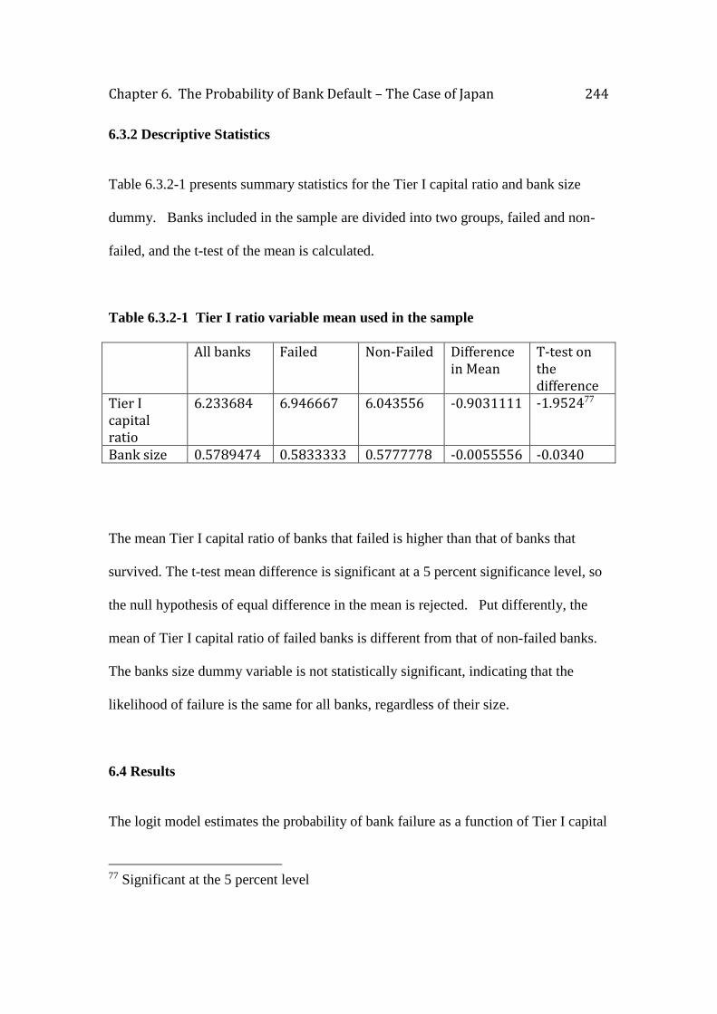
Chapter 6. The Probability of Bank Default – The Case of Japan 244
6.3.2 Descriptive Statistics
Table 6.3.2-1 presents summary statistics for the Tier I capital ratio and bank size
dummy. Banks included in the sample are divided into two groups, failed and non-
failed, and the t-test of the mean is calculated.
Table 6.3.2-1 Tier I ratio variable mean used in the sample
All banks Failed Non-Failed Difference in Mean
T-test on the difference
Tier I capital ratio
6.233684 6.946667 6.043556 -0.9031111 -1.952477
Bank size 0.5789474 0.5833333 0.5777778 -0.0055556 -0.0340
The mean Tier I capital ratio of banks that failed is higher than that of banks that
survived. The t-test mean difference is significant at a 5 percent significance level, so
the null hypothesis of equal difference in the mean is rejected. Put differently, the
mean of Tier I capital ratio of failed banks is different from that of non-failed banks.
The banks size dummy variable is not statistically significant, indicating that the
likelihood of failure is the same for all banks, regardless of their size.
6.4 Results
The logit model estimates the probability of bank failure as a function of Tier I capital
77 Significant at the 5 percent level

Chapter 6. The Probability of Bank Default – The Case of Japan 245
ratio, banks size dummy78 and year dummies79. The latter are included in the model to
allow the intercept to differ across years. The results of the estimated logit model80 are
presented below:
Table 6.4-1 Logit Model
Coefficient Robust SE Marginal effect
Tier I capital ratio 0.528** 0.248 0.077
Year dummy:
1999
0.760 1.002 0.001
Year dummy:
2000
0.421 1.183 0.065
Bank size dummy 0.648 0.632 0.092
Constant -5.595* 1.767 -
Number of observations= 57; Wald Χ2(4)= 8.43; p> Χ2=0.07; pseudo R2=.094;
log-likelihood= -26.570
*, **, Correspond to the 1% and 5% significance level, respectively
As in the case of US, the coefficient associated with Tier I capital ratio is positive and
statistically significant. This positive relationship implies that banks with higher
79 The base year is 1998 80 The Pearson X2 goodness of fit test used reveals that the number of covariate patters
is the same as the number of observations therefore the Hosmer and Lemeshow
goodness of fit test with 10 groups is used. The Homser and Lemeshow goodness of
fit, obtained by calculating the percentiles of the estimates probabilities, shows that
the model fits the data reasonably well. The output of the test are as follows: X2 (8)=
=8.53, prob>X2= 0.38 (See Appendix 5)
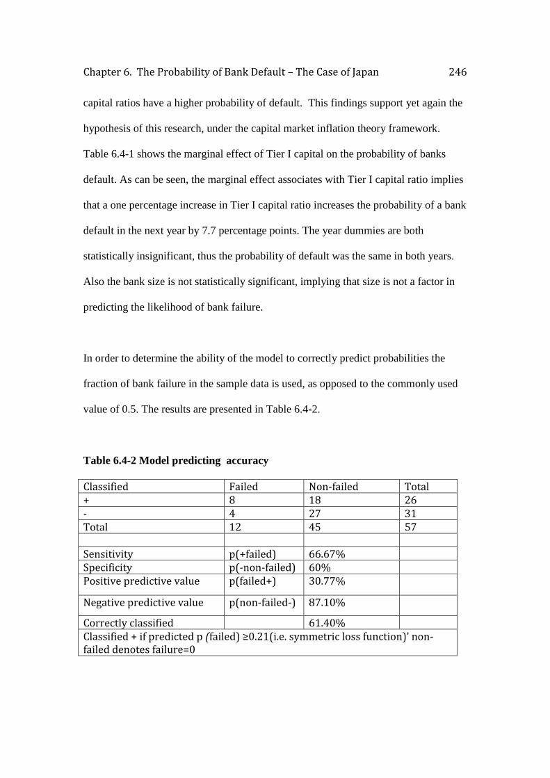
Chapter 6. The Probability of Bank Default – The Case of Japan 246
capital ratios have a higher probability of default. This findings support yet again the
hypothesis of this research, under the capital market inflation theory framework.
Table 6.4-1 shows the marginal effect of Tier I capital on the probability of banks
default. As can be seen, the marginal effect associates with Tier I capital ratio implies
that a one percentage increase in Tier I capital ratio increases the probability of a bank
default in the next year by 7.7 percentage points. The year dummies are both
statistically insignificant, thus the probability of default was the same in both years.
Also the bank size is not statistically significant, implying that size is not a factor in
predicting the likelihood of bank failure.
In order to determine the ability of the model to correctly predict probabilities the
fraction of bank failure in the sample data is used, as opposed to the commonly used
value of 0.5. The results are presented in Table 6.4-2.
Table 6.4-2 Model predicting accuracy
Classified Failed Non-failed Total + 8 18 26 - 4 27 31 Total 12 45 57 Sensitivity p(+failed) 66.67% Specificity p(-non-failed) 60% Positive predictive value p(failed+) 30.77%
Negative predictive value p(non-failed-) 87.10%
Correctly classified 61.40% Classified + if predicted p (failed) ≥0.21(i.e. symmetric loss function)’ non-failed denotes failure=0
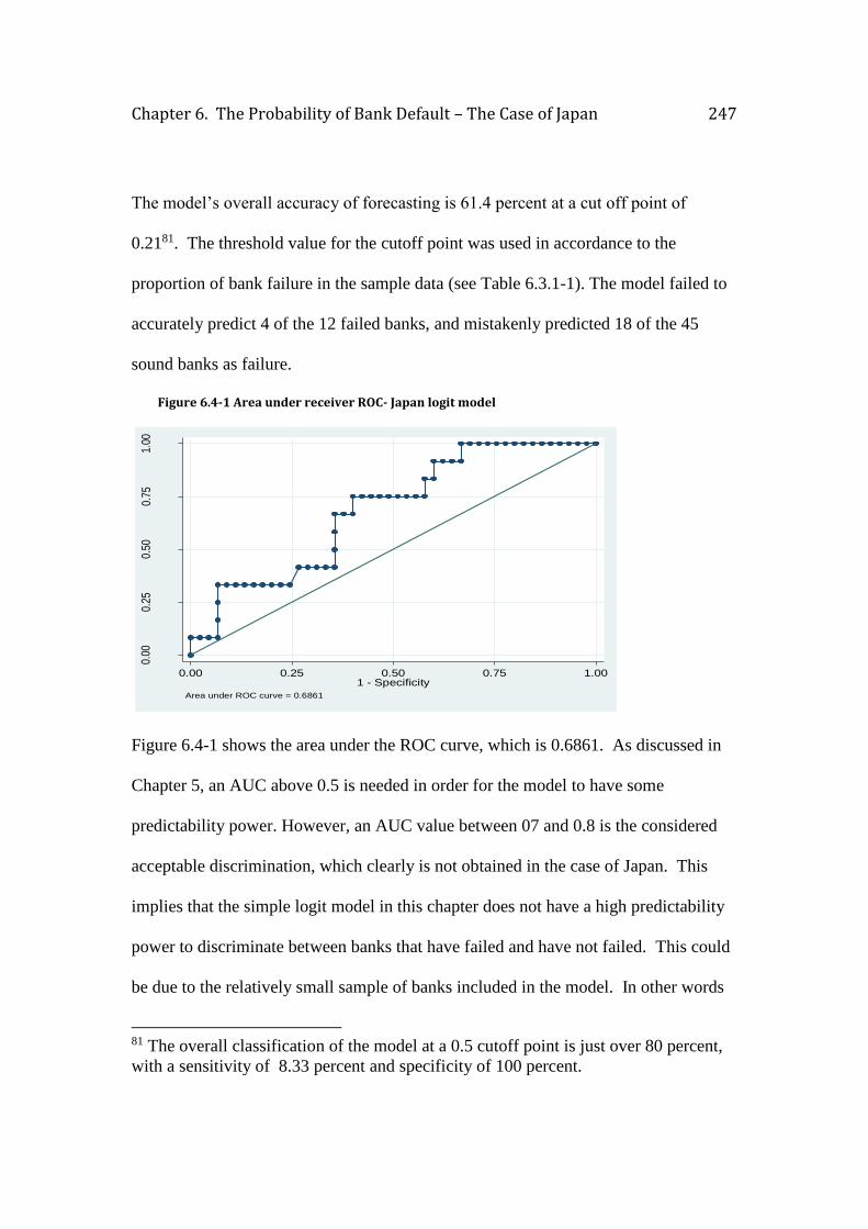
Chapter 6. The Probability of Bank Default – The Case of Japan 247
The model’s overall accuracy of forecasting is 61.4 percent at a cut off point of
0.2181. The threshold value for the cutoff point was used in accordance to the
proportion of bank failure in the sample data (see Table 6.3.1-1). The model failed to
accurately predict 4 of the 12 failed banks, and mistakenly predicted 18 of the 45
sound banks as failure.
Figure 6.4-1 Area under receiver ROC- Japan logit model
Figure 6.4-1 shows the area under the ROC curve, which is 0.6861. As discussed in
Chapter 5, an AUC above 0.5 is needed in order for the model to have some
predictability power. However, an AUC value between 07 and 0.8 is the considered
acceptable discrimination, which clearly is not obtained in the case of Japan. This
implies that the simple logit model in this chapter does not have a high predictability
power to discriminate between banks that have failed and have not failed. This could
be due to the relatively small sample of banks included in the model. In other words
81 The overall classification of the model at a 0.5 cutoff point is just over 80 percent,
with a sensitivity of 8.33 percent and specificity of 100 percent.
0.00
0.25
0.50
0.75
1.00
Sen
sitiv
ity
0.00 0.25 0.50 0.75 1.001 - Specificity
Area under ROC curve = 0.6861

Chapter 6. The Probability of Bank Default – The Case of Japan 248
the small sample may be a factor that limits the ability of the model to accurately
discriminate between failed and non-failed banks.
6.5 Concluding remarks
The empirical evidence of both Japanese and US bank failures presented in this
chapter and the previous one support the hypothesis of this research, that a bank with
higher capital ratio has a higher probability of default than a bank with a lower Tier I
capital ratio. These findings are in contrast with the common belief that higher capital
ratios serve as a cushion to withstand any unanticipated losses, thus lowering banks
probability of default. It has been argued that the reason for this is that, when banks
raise capital by issuing equity under conditions of capital market deflation, they drain
out the long-term finance that corporations need to conduct their business operations,
thus limiting their productive investment potential.
Another common characteristic of the crisis in Japan in the 1990s and in US in 2007-
09 is the subsequent lower productive investment by firms in both countries. In
relation to Japan, Shimziu (2007) argues that when regulators impose higher capital
requirements banks reduce their lending to firms so firms reduce their investment.
Toporowski argues that firms that cannot refinance their debts into equity reduce

Chapter 6. The Probability of Bank Default – The Case of Japan 249
investment. In the case of Japan this phenomenon is more evident and linked to debt
overhang from dissolution of keiratsu explained above.
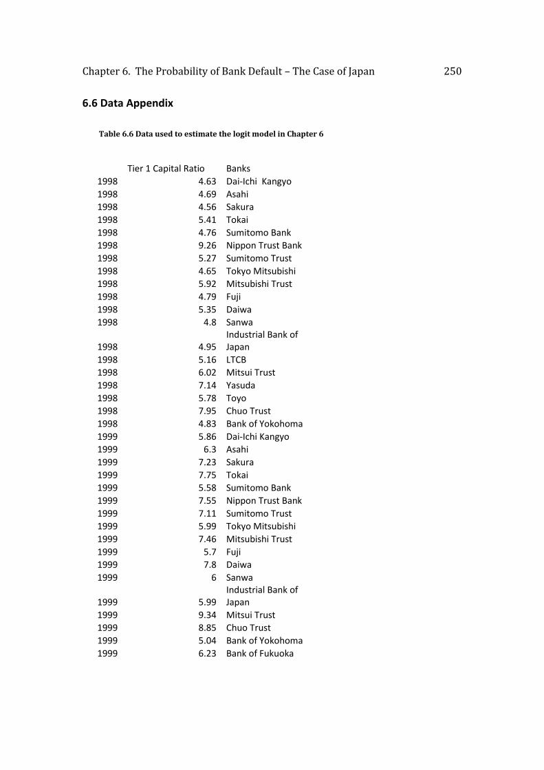
Chapter 6. The Probability of Bank Default – The Case of Japan 250
6.6 Data Appendix
Table 6.6 Data used to estimate the logit model in Chapter 6
Tier 1 Capital Ratio Banks
1998 4.63 Dai-Ichi Kangyo
1998 4.69 Asahi
1998 4.56 Sakura
1998 5.41 Tokai
1998 4.76 Sumitomo Bank
1998 9.26 Nippon Trust Bank
1998 5.27 Sumitomo Trust
1998 4.65 Tokyo Mitsubishi
1998 5.92 Mitsubishi Trust
1998 4.79 Fuji
1998 5.35 Daiwa
1998 4.8 Sanwa
1998 4.95 Industrial Bank of Japan
1998 5.16 LTCB
1998 6.02 Mitsui Trust
1998 7.14 Yasuda
1998 5.78 Toyo
1998 7.95 Chuo Trust
1998 4.83 Bank of Yokohoma
1999 5.86 Dai-Ichi Kangyo
1999 6.3 Asahi
1999 7.23 Sakura
1999 7.75 Tokai
1999 5.58 Sumitomo Bank
1999 7.55 Nippon Trust Bank
1999 7.11 Sumitomo Trust
1999 5.99 Tokyo Mitsubishi
1999 7.46 Mitsubishi Trust
1999 5.7 Fuji
1999 7.8 Daiwa
1999 6 Sanwa
1999 5.99 Industrial Bank of Japan
1999 9.34 Mitsui Trust
1999 8.85 Chuo Trust
1999 5.04 Bank of Yokohoma
1999 6.23 Bank of Fukuoka
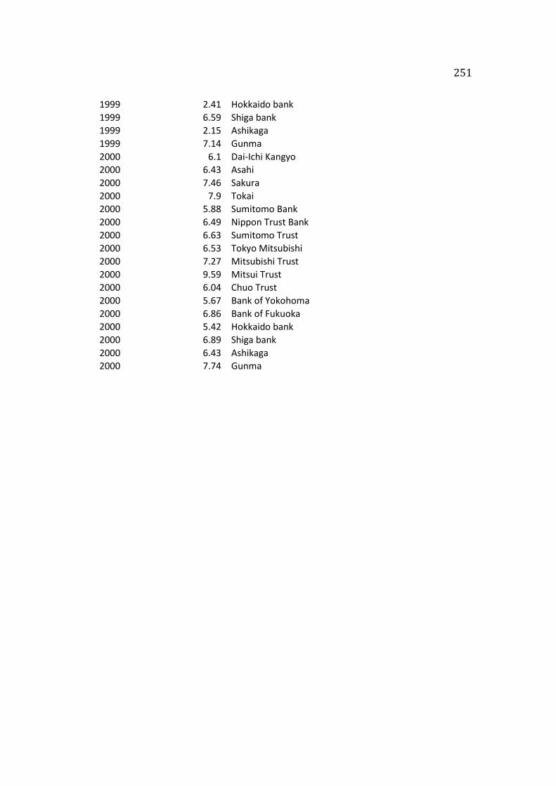
251
1999 2.41 Hokkaido bank
1999 6.59 Shiga bank
1999 2.15 Ashikaga
1999 7.14 Gunma
2000 6.1 Dai-Ichi Kangyo
2000 6.43 Asahi
2000 7.46 Sakura
2000 7.9 Tokai
2000 5.88 Sumitomo Bank
2000 6.49 Nippon Trust Bank
2000 6.63 Sumitomo Trust
2000 6.53 Tokyo Mitsubishi
2000 7.27 Mitsubishi Trust
2000 9.59 Mitsui Trust
2000 6.04 Chuo Trust
2000 5.67 Bank of Yokohoma
2000 6.86 Bank of Fukuoka
2000 5.42 Hokkaido bank
2000 6.89 Shiga bank
2000 6.43 Ashikaga
2000 7.74 Gunma
252
Chapter 7. Conclusion
This thesis has empirically examined the impact of capital adequacy regulation on the
probabilities of bank default and has theoretically analysed the impact of such
regulation on the economy as a whole. The analysis began by giving an overview of
how the capital markets actually work, with a particular focus on explaining how it
links the sectors of the economy. Understanding such link and the market conditions
in which banks operate provides a platform from which the impact of the Basel
capital requirements on banks at an individual level can be examined.
The US and Japan case studies chosen in this thesis to examine the impact of capital
adequacy regulation on the probabilities of bank default are not without intention.
Firstly is the large number of bank failures during the periods under consideration, US
during the latest crisis starting in 2007 and Japan during the 1990s, which has perhaps
been the most revealing hint in doubting the effectiveness of capital adequacy
regulation in promoting a safe and sound financial system. The large number of bank
failures occurred despite the fact that most banks not only met the Basel capital
standards, but also held capital in excess to the regulatory requirements. Secondly,
during these periods, the banking crisis and the subsequent recessions, both countries
experienced a significant decline in private investment. The previously inflated

Chapter 7. Conclusion 253
capital markets fostered a delusion that capital adequacy is the most effective
prudential regulation of the banking system.
This concluding chapter provides a concise summary of the research conducted in this
thesis. The evidence provided in this thesis suggests that capital adequacy regulation
gives misleading signals about the soundness of banks. Therefore, it is argued that
such regulation is theoretically flawed, taking no account how banks are
overcapitalised, or put differently it takes no account of balance sheet reconstruction
to achieve overcapitalisation. Some of the implications associated with the current
framework of bank capital regulation are discussed in section 2. Section 3 reflects on
the empirical results presented in this thesis, and provides recommendations for future
regulatory capital requirements, using the ideas put forward by both Toporowski and
Minsky.
7.1 Summing up
This thesis consists of 7 chapters. The first chapter gave an outline of the objectives,
motivations, the methodological approach and the structure of the thesis. The second
chapter gave an historical background of the Basel Accords, together with the
literature review on capital adequacy regulation. Two fundamental flaws were
identified in this chapter in relation to the existing literature: the first one is the lack of
the literature in providing empirical evidence on the impact of Tier I capital ratios on
the probabilities of bank default and the second one concerns the lack of the literature
Chapter 7. Conclusion 254
in providing an analysis of the impact of such regulation that considers the economic
system as a whole.
Chapter 3 presented a detailed explanation of the theoretical aspects of the capital
market inflation theory. It then developed a simple model to estimate stock price
movements taking into account the net excess inflows into the capital market. The net
excess inflows is calculated using the demand and supply for equity capital, derived
from the flow of funds accounts. The demand for equity capital represents issues of
equity capital from the non-financial and financial sector. The supply for equity
capital represents purchases of corporate equity from the household, institutional
investors and the external sector. The results of the time series regression provide
evidence that the excess supply of capital does affect stock price movements.
However, whilst these results empirically validate the assumptions of the capital
market inflation theory when applied to the US, the model does not yield the same
results when applied to the Japanese capital market. Various factors were highlighted
which could explain such results. In particular the Japanese central bank purchases of
shares and other equities were argued and shown empirically to have a positive effect
on the Nikkei 225 stock price index. This on the other hand suggests that these
purchases offset private sector outflows of credit form the capital market. Therefore,
capital market inflation theory may still be valid in this case.
The purpose of this chapter was to provide a platform from which the effectiveness of
the capital adequacy regulation in promoting the soundness of the banking sector can
Chapter 7. Conclusion 255
be examined. An effective analysis for banking distress cannot be conducted by
considering the banking sector in isolation from the other sectors in the economy.
Therefore it is imperative to understand how a capitalist economy works, the
development is other sectors of the economy and how these sectors are linked, in
order to better examine the behaviour and soundness of banks, given any capital
regulatory restrictions.
From a macro-perspective the capital market inflation theory argument is that in
conditions of capital supply rationing bank overcapitalisation makes the financial
system in general more fragile, because it crowds out available capital for non-
financial firms. This fragility then appears as growing risky debt in the banking
system. This statement, which is supported empirically in this thesis, is then used to
explain the probability of default of individual banks.
The discussion on the shadow banking system, presented in chapter 4, enters as a way
in which banks ‘dress-up’ their balance sheets by transferring those risky assets in the
non-bank subsidiaries. In this way shadow banking, provides an explanation of how
banks respond to the growing riskiness of their assets.
Chapter 5 provides an empirical evaluation of the relationship between capital
adequacy ratios, and the probability of default of US banks. The analysis employs a
logit model to estimate the probability of bank default on a pooled cross sectional data
over the period 2007-2009. The results imply that a 1 percentage point in Tier I
Chapter 7. Conclusion 256
capital ratios increases the probability of default by 1.8 percentage points. In contrary
a 1 percentage point increase in the unweighted capital ratios lowers the probability of
default by 2.7 percentage points. It was argued that the unweighted capital ratio
coefficient is the effect of illiquidity in the market for relatively risk-free assets,
whereas the risk-weighted capital ratio, i.e. Tier 1 capital ratio, is the effect of
crowding out in the capital market. In other words the current risk-weighted capital
requirement account only for risk of insolvency, ignoring the risk of illiquidity in the
capital market.
Similarly, chapter 6 provides empirical evidence on the impact of capital adequacy
regulation on the probability of default of Japanese banks, over the period 1998-2000,
using the same methodology as in chapter 5. However, due to data limitation only
risk-weighted capital ratio was used to estimate the probability of bank default. The
results indicate that when Tier I capital ratio is increased by 1 percentage point, banks
probability of default increases by 7.7 percentage points.
7.2 Some further comments
This thesis has provided empirical evidence arguing against the capital adequacy
regulation currently placed on banks. However, despite this, it is of great importance
to stress that in this thesis, these results do not provide evidence against such
regulation per se. Rather these results provide evidence against the framework of
capital adequacy regulation. In other words this thesis does not advocate restricting
banking regulation, i.e. a lighter regulatory regime, but it rather argues that any
Chapter 7. Conclusion 257
regulatory restrictions placed on banks need to take into account developments in
other sectors of the economy and on the fringes of the banking system itself.
The banking sector is closely connected to all sectors in the economy, by means of
providing credit and liquidity. Perhaps the most important role of all of the banking
sector, is the provision of credit to facilitate investment expenditure, with the latter
being a crucial component of aggregate demand. Therefore, any factor limiting the
willingness and ability of banks to increase the money supply and credit is bound to
have a direct effect of the level of investment, and hence on economic activity.
However the banking sector is connected with other sectors in the economy also on its
liability side, especially in the most developed economies, as argued in this thesis.
This way, in which the activities of the banking sector affect the rest of the economy
should not be ignored.
7.3 Recommendations for future regulatory capital standards
As outlined above this thesis argues that capital adequacy regulation is theoretically
flawed. Therefore, this thesis suggests that theory on banking regulation needs to
move beyond an unsophisticated model of a single bank balance sheet to a more
complex view of how bank balance sheets are integrated with other balance sheet in
the economy. This section borrows the ideas put forward by Toporowski and Minsky
to provide recommendations that should be taken into account when placing
regulatory standards on banks.
Chapter 7. Conclusion 258
As a recommendation tool for banking regualtion, an important argument that is
derived from Toporowski’s argument against the Basel capital requirements is bank
heterogeneity. He states that ‘The strategy of securing banks stability by enforcing
capital adequacy is based on a fallacy of composition: what is good for one bank is
not necessarily good for all banks taken together’ (Toporowski 2009, pg. 1). This line
of reasoning is also given by Minsky (1967, 1975a). As explained in chapter 2,
Minsky suggests a bank examination approach in order to determine an exact
appropriate level of capital and liquidity for a bank. His argument is built upon the
suggestion that each bank needs to be assessed individually. Minsky states ‘the
liquidity of an institution cannot be measured by assigning universal predetermined
liquidity quotients to assets and similar liquidity requirement factors to liability’
(Minsky 1967, pg.6). However, the information obtained from each bank then needs
to be incorporated with market aggregates. That is because, ‘liquidity is not an innate
attribute of an asset but rather that liquidity is a time related characteristic of an
ongoing, continuing economic institutions’ (Minsky 1967, pg. 6).
In order to better determine the liquidity needs of a particular bank it is necessary not
only to examine its initial balance sheet but also to estimate cash flows taking into
account future economic conditions that are likely to effect the banks’ ability to adjust
its cash position82. This way, regulatory bodies would be better informed not only on
the financial position of a particular bank but also would have a more in depth
82 Minsky notes that banks generate cash flows not only from ordinary operations but
also by operating in asset and liability markets. He refers to the activities that banks
undertake to adjust their cash position as position- making activities.
Chapter 7. Conclusion 259
knowledge on their operation activities as well as on their interactions with other
financial institutions, and most importantly with shadow banks which Minsky called
‘fringe banks’. The importance of the latter point was highlighted in Chapter 4, in
which it was argued that prior to the 2008 financial crisis US regulatory bodies had
little knowledge on the banks interactions with the shadow banking system.
Examining bank’s balance sheet will not only serve to gather accurate information
about the position making ability of a particular bank and the interactions with other
financial institutions but will also reveal the connections it has with other sectors in
the economy. When all data is generated for each individual bank is then aggregated
to give a real picture of all markets in which banks operate.
This thesis advocates a banking framework proposed by Minsky, which recognizes
that the ability of banks to convert assets into cash, thereby the ability of banks to be
liquid is more important than raising capital, which has major implications for the
productive investment process by non-financial corporations. But this is not to say
that this is the full remedy for promoting stability in the economy. Whilst regulating
the banking sector is indeed an importance task for governments, other sectors in the
economy could also benefit from government monitoring. The monitoring process
here is meant to say, not heavily regulating for example the non-financial corporate
sector or institutional investors, but is intended to say that if governments were better
informed on their business activities it can give them better information and assist in
finding ways to discourage their over-reliance on the financial markets to continue
their business operations. As Toporowski (2009b) states, ‘Economic activity must be

Chapter 7. Conclusion 260
reorganised to make the real economy more stable and financial markets more boring,
so that enterprise is focussed on innovations that enhance welfare, rather than
financial inflation’ (2009, pg. 9).
261
9. Bibliography
Admati, A., and Hellwig, M., (2013), The Bankers’ New Clothes, What’s Wrong with
Banking and What to Do about It, Princeton: Princeton University Press
Adrian, T., and Ashcraft, A., (2012a), Shadow Banking: A Review of the Literature,
Federal Reserve Bank of New York, Staff Report No.580
Adrian, T., and Ashcraft, A., (2012 b), Shadow Banking Regulation, Federal Reserve
Bank of New York, Staff Report No.559
Adrian, T., Burke, Ch., and McAndrews, J., (2009), The Federal Reserve’s Primary
Dealer Credit Facility, Federal Reserve Bank of New York Current Issues in
Economics and Finance, Vol.15, No. 4
Allen, F., (1996), The Future of the Japanese Financial System, Working Paper,
Financial Institutions Centre, The Wharton School, University of Pennsylvania
Alfon, I., Argimon, I., and Bascunana-Ambros, P., (2004), What determines how
much capital is held by UK banks and building societies?, Financial Services
Authority, Occasional Paper Series 22
Allen, L., (2003), The Basel Capital Accords and International Mortgage Markets: A
Survey of the Literature, New York University Salomon Centre, Financial Markets,
Institutions & Instruments, Vol. 13, Issue. 2, pp.41-108,
available on: http://pages.stern.nyu.edu/~lallen/mortgage.paper.pdf
9. Bibliography 262
Alvarez, G., S., (2010), The Acquisition of Wachovia Corporation by Wells Fargo &
Company, Before the Financial Crisis Inquiry Commission, The Federal Reserve
Bank, Testimony, available from:
http://www.federalreserve.gov/newsevents/testimony/alvarez20100901a.htm
Aktas, R., Doganay, M., and Ceylan, N., (2006), Predicting Financial Failure of the
Turkish Banks, Annals of Financial Economics , Vol. 2. Issue 1
Asteriou, D., and Hall, S., (2007), Applied Econometrics, A modern Approach, New
York: Palgrave macmillian, Revised Edition
Bank of America (2011), Asset-Backed Commercial Paper: A Primer, BofA Global
Capital Management
Barrell, R., Davis, E. P., Fic, T., Holland, D., Kirby, S., and Liadze, I., (2009),
Optimal regulation of bank capital and liquidity: how to calibrate new international
standards, Financial Services Authority, Occasional Paper Series 38
Barsky. R., (2009), The Japanese Bubble: A “Heterogeneous’ Approach, NBER
Working Paper 15052
Baur, B., and Wackerbeck, Ph., (2013), Into the Shadow: How regulation fuels the
growth of the shadow banking sector and banks need to react, The European
Financial Review, June-July 2013
BBC News, (2009), Timeline: Credit Crunch to Downturn, available on :
http://news.bbc.co.uk/1/hi/7521250.stm
BCBS (1988), International Convergence of Capital Measurements and Capital
Standards, Bank for International Settlements
9. Bibliography 263
BCBS (2009a), Revision to the Basel II Market Risk Framework, Bank for
International Settlements
BCBS (2009b), Guidelines for Computing Capital for Incremental Risk in the Trading
Book, Bank for International Settlements, January
BCBS(2010a), Basel III: A Global Regulatory Framework for More Resilient Banks
and Banking Systems, Bank for International Settlements, December
BCBS (2010b), Basel III: International Framework for liquidity Risk Measurements,
Standards and monitoring, Bank for International Settlements
BCBS (2010c), International Framework for Liquidity Risk Measurements, Standards
and Monitoring, Bank for International Settlements, December
BCBS(2010d), An Assessment of the Long-Term Economic Impact of Stronger
Capital and Liquidity Requirements, Bank for International Settlements, August
BCBS (2011), Global Systemically Important Banks: Assessment Methodology and
the Additional Loss Absorbency Requirement, Bank for International Settlements
BCBS (2012), Fundamental Review of the Trading Book, Consultative document,
Bank for International Settlements
Bou-Said, M., and Saucier, Ph., (2003), Liquidity, Solvency and Efficincy? An
Empirical Analysis of the Japanese Banks’ Distress, in 20th Symposium on Banking
and Monetary Economics, Universite d’Orleans and University of Birmingham
9. Bibliography 264
BIS, (2001), The New Basel Capital Accord: an explanatory note, Bank for
International Settlements, Secretariat of the Basel Committee on Banking Supervision
Blinder, A., (2013), After the Music Stopped,: The Financial Crisis, the Response and
the Work Ahead , New York: Penguin Press
Blum, J., (1999), Do Capital Adequacy Requirements Reduce Risks in Banking?
Journal of Banking and Finance 23, pp.755-771
Borio, C., (2003), Toward a Macroprudential Framework for Financial Supervision
and Regulation?, BIS Working Papers, No.128, February
Borio, C., (2011), Rediscovering the Macroeconomic Roots of Financial Stability
Policy: Journey, Challenges and a Way Forward, BIS Working Papers, No. 354,
September
Bunn, Ph., and Redwood, V., (2003), Company accounts based modelling of business
failures and the implication for financial stability, Bank of England, Working Paper
No. 210
Campbell, D., (2009), UCBH Holdings’ Bank is Seized, 120th U.S. Lender Shut This
Year, Bloomberg, available on
http://www.bloomberg.com/apps/news?pid=newsarchive&sid=ayPwsBV1DI3c
Capie, F., and Wood, G., ( 2013), Do We Need Regulation of Bank Capital? Some
Evidence From the UK, IEA Current Controversies No.40
CBO (2010), Fannie Mae, Freddie Mac, and the Federal Role in the Secondary
Mortgage Market, Congress of the Unites States, Congressional Budget Office
9. Bibliography 265
Chicago Tribune., (2000), Japanese Banks Planning to Form $1 Trillion Institution,
available on: http://articles.chicagotribune.com/2000-03-
15/business/0003150380_1_asahi-bank-banking-analyst-mizuho-financial-group
CNNMoney, (1999), Sumitomo, Sakura to Merge, available from:
http://money.cnn.com/1999/10/14/asia/japan_banks/
Citigroup (2013), Citigroup Inc. Basel II.5 Market Risk Disclosures AS of and For the
Period Ended June 30, 2013, available on:
http://citigroup.com/citi/investor/data/b25d130630.pdf
Cole, A. R., and Gunther, W. J., (1998), Predicting Bank Failures: A Comparison of
On-and Off-Site Monitoring Systems, Journal of Financial Services Research 13:2,
pp. 103-117
Condon, Ch., (2008), Money-Market Fund “Breaks the Buck”, The Washington Post,
available on:
http://www.washingtonpost.com/wp-
dyn/content/article/2008/09/16/AR2008091603422.html
Copeland, A., Duffie, D, Martin, A., and McLaughlin, S., (2012), Key Mechanics of
the U.S. Tri-Party Repo Market, Federal Reserve Bank of New York, Staff Report
No. 477
Coppola, F., (2013), The Equivalence of Debt and Equity, Coppola Comment:
Finance, Economics and Music, available on :
http://coppolacomment.blogspot.co.uk/2013/05/the-equivalence-of-debt-and-
equity.html
9. Bibliography 266
Corbett, J., and Jenkinson, T., (1994), The Financing of Industry, 1970-1989: An
International Comparison, Journal of the Japanese and International Economies 10,
71-96
Corbett, J., and Jenkinson, T., (1997), How is investment financed? A study of
Germany , Japan, the United Kingdom and the United States, Manchester School,
65:69-93
Crockett, A., (2000), Marrying the micro-and macroprudential dimensions of
financial stability, BIS Speeches, 21 September
Davis, E. P., and Karim, D., (2008), Comparing Early Warning Systems for Banking
Crises, Journal of Financial Stability, Vol. 4, pp. 89-120
Davies, J. P., and Sakoui, A., (2008), Sigma Collapse Marks End of SIV Era,
Financial Times, available on : http://www.ft.com/cms/s/0/18fbcd5c-8fe4-11dd-9890-
0000779fd18c.html#axzz2rSIy6QzT
Dealbook (2008), Capital One to Buy Chevy Chase Bank, The New York Times,
available on: http://dealbook.nytimes.com/2008/12/04/capital-one-may-acquire-a-
rival-bank/?_r=0
Demirguc-Kunt, A., and Detragiache, E., (1998), The Determinants of Banking
Crises in Developing and Developed Countries, IMF Staff Paper, Vol. 45, No.1
D’Hulster, K., (2009), The Leverage Ratio A New Binding Limit on Banks, The
World Bank Group, Financial and Private Sector Development Vice Presidency, Note
Number 11
9. Bibliography 267
Diamond, D., and Dybvig, Ph., (1983), Bank Runs, Deposit Insurance, and Liquidity,
The Journal of Political Economy, Vol. 91, No.3, pp. 401-419
Dolbeare, H., and Barnd, M., (1931), Forewarnings of bank failures: A comparative
study of the statements of certain failed and successful Florida state banks, 1922-
1928. Gainesville, FL: University of Florida Business Administration Series (1)
Dymski, G., (1988), A Keynesian Theory of Bank Behaviour, Journal of Post
Keynesian Economics, Vol.10, No.4, pp. 499-526
Economic Science Prize Committee of Royal Swedish Academy of Science (2013),
Understanding Asset Pricing, available on:
http://www.nobelprize.org/nobel_prizes/economic-sciences/laureates/2013/advanced-
economicsciences2013.pdf
Ediz, T., Michael, I., and Perraudin, W., (1998), The impact of capital requirements
on U.K. bank behaviour, FRBNY Economic Policy Review/ October 1998
Elliot, J. D., (2010), Quantifying the effects on lending of increase capital
requirements, The Brookings Institutions
Ellis, D., (2008), Washington Mutual Loses $3.3 billion, CNNMoney, available on:
http://money.cnn.com/2008/07/22/news/companies/wamu/?postversion=2008072219
Engel, K., and McCoy, P., (2011), The Subprime Virus: Reckless Credit, Regulatory
Failure, and Next Steps, Oxford University Press, available on:
http://papers.ssrn.com/sol3/papers.cfm?abstract_id=1762869
9. Bibliography 268
Emmons, W., Lskavyan, V., and Yeager, T., (2005), Basel II Will Trickle down to
Community Bankers, Consumers, Federal Reserve Bank of ST. Louis, The Regional
Economist, available on: http://www.stlouisfed.org/publications/re/articles/?id=363
Epstein, G., (2005), Financialization and the Word Economy, Edward Elgar
Publishing
Estrella, A., Park, S., and Peristani, S., (2000), Capital Ratios as Predictors of Bank
Failure, FRBNY Economic Policy Review, July 2000
Fama, E., Fisher, L., Jensen, M and Roll., R., (1969), ‘The Adjustment of Stock
Prices to New Information’, International Economic Review, Vol.10, No.1, pp. 1-21.
Farhi Maryse et Marcos Antonio Macedo Cintra, (2009), The Financial Crisis and the
Global Shadow Banking System, Revue de la regulation, No.5
FASB, (2009), Briefing Document : FASB Statement 166 and 167, available on :
http://www.fasb.org/cs/ContentServer?c=FASBContent_C&pagename=FASB%2FFA
SBContent_C%2FNewsPage&cid=1176155633483
The Federal Reserve Bank of New York, (2010), Tri-Party Infrastructure Reform,
White Paper, available on :
http://www.newyorkfed.org/banking/nyfrb_triparty_whitepaper.pdf
Federal Reserve, (2008), Asset-Backed Commercial Paper (ABCP) Money Market
Mutual Fund (MMMF) Liquidity Facility (AMLF), Press Release, available on:
http://www.federalreserve.gov/newsevents/press/monetary/20080919a.htm
Federal Reserve, (2010), Commercial Paper Funding Facility, available on :
http://www.federalreserve.gov/monetarypolicy/cpff.htm
9. Bibliography 269
Federal Reserve, (2014), Agencies Adopt Enhanced Supplementary Leverage Ratio
final rule and Issue Supplementary Leverage Ratio Notice of Proposed Rulemaking,
Joint Press Release, available on :
http://www.federalreserve.gov/newsevents/press/bcreg/20140408a.htm
FDIC, (1997), History of the Eighties: Lessons for the Future, Volume 1, Chapter 4
Available on: https://www.fdic.gov/bank/historical/history/167_188.pdf
FDIC, (2007), FDIC Approves The Assumption of The Insured Deposits of Netbank,
Alpharetta Georgia, FDIC Press Releases, available on:
https://www.fdic.gov/news/news/press/2007/pr07081.html
FDIC, (2008a), JPMorgan Chase Acquires Banking Operations of Washington
Mutual, FDIC Press Releases, available on:
http://www.fdic.gov/news/news/press/2008/pr08085.html
FDIC, (2008b), U.S. Bank Acquires All Deposits of Two Southern California
Institutions, Downey Savings & Loan Association, Newport Beach and PFF Bank &
Trust, Pomona, FDIC Press Releases, available on:
http://www.fdic.gov/news/news/press/2008/pr08124.html
FDIC, (2009a), FDIC Closes Sale of IndyMac Federal bank, Pasadena, California,
FDIC Press Releases, available on:
http://www.fdic.gov/news/news/press/2009/pr09042.html
FDIC, (2009b), BBVA Compass, Birmingham, Alabama, Assumes All of the
Deposits of Guaranty Bank, Austin, Texas, FDIC Press Releases, available on:
https://www.fdic.gov/news/news/press/2009/pr09150.html
9. Bibliography 270
FDIC, (2009c), BB&T, Winston-Salem, North Carolina, Assumes All of the Deposits
of Colonial Bank, Montgomery, Alabama, FDIC Press Releases, available on :
http://www.fdic.gov/news/news/press/2009/pr09143.html
FDIC (2009d), New York Community Bank, Westbury, New York, Assumes All of
the Deposits of AMTrust Bank, Cleveland, Ohio, FDIC Press Releases, available on:
http://www.fdic.gov/news/news/press/2009/pr09222.html
FDIC,(2010), $250,000 Federal Deposit Insurance Amount Now Permanent, FDIC
Consumer News, available on :
http://www.fdic.gov/consumers/consumer/news/cnsum10/250k_fed_deposit_insuranc
e.html
FDIC (2012), Regulatory Capital Rules: Standardized Approach for Risk-Weighted
Assets; Market Discipline and Disclosure Requirements, Financial Institution Letters,
available on : http://www.fdic.gov/news/news/financial/2012/fil12027.html#cont
FDIC, (2013), Risk Retention Re-Proposal: Application to ABCP Conduits, available
on: http://www.fdic.gov/regulations/laws/federal/2013/2013-credit_risk_retention-
staff_01-supp.pdf
Financial Services Authority, (2011), Assessing the Possible Sources of Systematic
Risk from Hedge Funds, London: Financial Services Authority
Fisher, I. (1933) ,The Debt Deflation Theory of Great Depressions. Econometrica
Vol. 1, No.1, pp.337-357.
9. Bibliography 271
FSB (2011), Shadow Banking: Strengthening Oversight and Regulation, Financial
Stability Board, available on:
http://www.financialstabilityboard.org/publications/r_111027a.pdf.
FSB (2013a), 2013 Update of Group of Global Systemically Important Banks (G-
SIBs), Financial Stability Board, available on :
https://www.financialstabilityboard.org/publications/r_131111.pdf
FSB, (2013b), Strengthening Oversight and Regulation of Shadow Banking, An
Overview of Policy Recommendations, Financial Stability Board, available on :
http://www.financialstabilityboard.org/publications/r_130829a.pdf
FSB, (2012), Global Banking Monitoring Report, Financial Stability Board, available
on : http://www.financialstabilityboard.org/publications/c_130129y.pdf
Foreman, R., D., (2002), A logistic analysis of bankruptcy within the US local
telecommunications industry, Journal of Economics & Business, 55, 135-166
Flath, D., (2005), The Japanese Economy, New York: Oxford University Press,
Second Edition
Fukao, M., (1998), Japanese Financial Instability and Weaknesses in the Corporate
Governance Structure, Seoul Journal of Economics, 11, pp. 381-422
Fukao, M., (2003), Financial Sector Profitability and Double-Gearing, In Blomstrom,
M., Corbett, J., Hayashi, F., and Kashyap, A., ed. Structural Impediments to Growth
in Japan, University of Chicago Press, pp. 9-35
Furfine, C., (2000), Evidence on the Response of US Banks to Changes in Capital
Requirements, BIS Working Paper, No. 88
9. Bibliography 272
Gale, K.,(2009), BankUnited Financial Corp. files for Chapter 11, South Florida
Business Journal , available on:
http://www.bizjournals.com/southflorida/stories/2009/05/18/daily74.html?page=all
Gale, D., (2010), Capital Regulation and Risk Sharing, International Journal of
Central Banking, 23, pp.187-204
GAO, (1996), Report to the Honourable Charles E. Schumer House of
Representatives, Bank Regulatory Structure Japan, United States General Accounting
Office
Gaytan, A., and Johnson, A. Ch., (2002), A Review of the Literature on Early
Warning Systems for Banking Crises, Central Bank of Chile, Working Papers, No.
183
Getter, D., (2014), U.S. Implementation of the Basel Capital Regulatory Framework,
Congressional Research Service R42744
Getter, D., (2012), U.S. Implementation of the Basel Capital Regulatory Framework,
Congressional Research Service 7-5700
Goldman, D., Luhby, T., and Wong, G., (2009), BofA: $20B bailout, huge Merrill
loss, CNN Money, available on:
http://money.cnn.com/2009/01/16/news/companies/bofa_new_bailout/
Gorton, G., (2010), Slapped by the Invisible Hand: The Panic of 2007, New York:
Oxford University Press
9. Bibliography 273
Gorton, G., (2012), Misunderstanding Financial Crisis: Why We Don’t See Them
Coming, New York: Oxford University Press
Gorton, G., and Souleles, N., (2006), Special Purpose Vehicles and Securitization, In
The Risk of Financial Institutions, edited by Stulz, R., and Carey, M., University of
Chicago Press,
Gorton, G., and Metric, A., (2009), Haircuts, NBER Working Paper Series, Working
Paper 15273
Gorton, G., and Metric, A., (2010), Regulating the Shadow Banking System,
Brookings Papers on Economic Activity (Fall), 261-297
Gorton, G., and Metric, A., (2012), Securitized Banking and the Run on Repo,
Journal of Financial Economics 104, 425-451
Gow, D., (2008), Profit Prediction Raises Hopes that UBS Will Put Through, The
Guardian, available on:
http://www.theguardian.com/business/2008/oct/03/ubs.creditcrunch
Granger, C.W.J., (1969), Investigating Causal Relations by Econometric Models and
Cross Spectral Methods, Econometrica, 35, pp.424-38
Guha, K., Guerrera, F., and Rappeport, A., (2009), Stress Test Show $75bn Buffer
Needed, Financial Times, available on: http://www.ft.com/cms/s/0/f67cd12c-3b23-
11de-ba91-00144feabdc0.html?siteedition=uk#axzz2zAz5umkY
Gullapalli, D., Anand, Sh., and Maxey, D., (2008), Money Fund, Hurt by debt Tied to
Lehman, Breaks the Buck, The Wall Street Journal, available on:
http://online.wsj.com/news/articles/SB122160102128644897

9. Bibliography 274
Harada, K., and Ito, T., (2008), Did Mergers Help Japanese Mega-Banks Avoid
Failure? Analysis of the Distance to Default of Banks, NBER Working Paper Series
Harada, K., and Ito, T., (2012), Mega-Mergers’ Economic Reasons and Performances:
Lessons from Japan, The Association of Korean Economic Studies, available on:
http://www.akes.or.kr/eng/papers(2012)/40.full.pdf
Harada, K., Ito, T., and Takahashi, Sh., (2013), Is the Distance to Default a Good
Measure in Predicting Bank Failures? A Case Study of Japanese Major Banks? ,
Japan and the World Economy 27, pp.-70-82
Harcourt, G., and Riach, P., (2005), The General Theory: Volume 2 Overview,
Extensions, Method and New Developments, Volume 2, London: Routledge
Harrington, D. Sh., and Hester, E., (2007), Citigroup to Consolidate Seven SIVs on
Balance Sheet (Update 3), Bloomberg available :
http://www.bloomberg.com/apps/news?pid=newsarchive&sid=aT0Ix2iDnZRk
Heffernan, S., (2005), Modern Banking, John Wiley & Sons, West Sussex, UK
Hein, E. (2011) Financialisation, Re-Distribution, and the Financial and Economic
Crisis – a Kaleckian Perspective, in T. Niechoj, Ö. Onaran, E. Stockhammer, A.
Hielscher, J., (2008), BankUnited’s Parent Says Future is in Doubt, Herald-Tribute,
available on:
http://www.heraldtribune.com/article/20081219/article/812190321?p=1&tc=pg&tc=a
r
9. Bibliography 275
Truger and T. van Treeck (eds.), Stabilising an Unequal Economy? Public Debt,
Financial Regulation, and Income Distribution, Marburg: Metropolis, 35-62
Hirota, Sh., (1999), Are Corporate financing Decisions Different in Japan? An
Empirical Study on Capital Structure, Journal of the Japanese and International
Economics, Vol.13, pp201-229
Hoshi, T., (2001), What Happened to Japanese Banks? Monetary and Economic
Studies/February 2001
Hoshi, T., and Kashyap, A., (2001), Corporate Financing and Governance in Japan:
The Road to the Future, Cambridge, MA: MIT Press
Hoshi, T., and Kashyap, A., (2004), Japan’s Financial Crisis and Economic
Stagnation, Journal of Economic Perspectives, Vol.18, No.1, pp. 3-26
Hoshi, T., and Kashyap, A., (1999), The Japanese Banking Crisis: Where Did It
Come From and How Will It End? NBER Working Paper 7250
Hosmer, D., and Lemeshow, S., (2004), Applied Logistic Regression, John Wiley &
Sons, Second edition
Hsu, H., and Lin, B., (2002), The Kinetics of the Stock Markets, Asia Pacific
Management Review, 7(1), 1-24
Hull, J., (2012), Risk Management and Financial Institutions, Hoboken, New Jersey
:John Wiley & Sons, Third Edition
Hutchison, M., and Westermann, F., (2006), Japan’s Great Stagnation: Financial and
Monetary Policy Lesson for Advanced Economics, MIT Press
9. Bibliography 276
IMF, (2011), World Economic Outlook: Tensions From the Two-Speed Recovery,
Global Prospects and Policies, IMF April 2011
Jagtiani, J., Kolari, J., Lemieux, C., and Shin, H., (2003), Early Warning Models for
Bank Supervision: Simpler Could be Better, Federal Reserve Bank of Chicago,
3Q/2003, Economic Perspectives
Jagtiani, J., Kolari, J., Lemieux, C., and Shin, H., (2000), The Determinants and Early
Detection of Inadequate Capitalization of U.S. Commercial Banks, Federal Reserve
Bank of Kansas City, available on:
https://www.kansascityfed.org/publicat/brp/2002_Kolari_Law_Journal.pdf
Jimenez, G., Ongena, S., Peydro, J-L., and Saurina, J., (2012) Macroprudential
Policy, Countercyclical Bank Capital Buffers and Credit Supply: Evidence from the
Spanish Dynamic Provisioning Experiments, Bank of Spain
Johnson, S., and Kwak, J., (2010), 13 Bankers, The Wall Street Takeover and the Next
Financial Crisis Meltdown, Vintage Books , A Division of Random House, Inc. New
York
Kahane, Y., (1977), Capital Adequacy and the Regulation of Financial Intermediaries,
Journal of Banking and Finance 14, pp. 35-58
Kalyanaraman, L., and Tuwajri, B., (2014), Macroeconomic Forces and Stock Prices:
Some Empirical Evidence from Saudi Arabia, International Journal of Financial
Research, Vol.5, No.1
Kaminsky, L. G., and Reinhart, C., (1999), The Twin Crises: The Causes of Banking
and Balance-of-Payments Problems, The American Economic Review, Vol. 89, no. 3
PP 473-500
9. Bibliography 277
Kanaya, A., and Woo, D., (2000), The Japanese Banking Crisis of the 1990s : Sources
and Lessons, IMF Working Paper
Kanaya, A., and Woo, D., (2001), The Japanese Banking Crisis of the 1990s: Sources
and Lessons, Essays in International Economics, No.222, and International
Economics Section of the Department of Economic Preston University
Kashyap, A., Hanson, S., and Stein, J., (2010), A Macroprudential Approach to
Financial Regulation, Journal of Economic Perspective, 25, No. 1, pp. 3-28
Kashyap, A., and Stein, J., (2004), Cyclical Implications of the Basel II Capital
Standards, Federal Reserve Bank of Chicago Economic Perspective 28, Q1, pp.18-31
Karwowski, E., and Shabani, M., (2014), Why do Dow Jones-Listed Companies
Hold Increasingly Cash Balances? The Impact of Financial Operations of Non-
financial Firms on Macroeconomic Stability, Growth and Policy Effectiveness,
(forthcoming)
Kawai, M.,(2003), Japan’s Banking System: From The Bubble And Crisis to
Reconstruction, PRI Discussion Paper Series No 03 A- 2 8
Keeley, M., (1988), Bank Capital Regulation in the 1980s: Effective or Ineffective?
Federal Reserve Bank of San Francisco, Economic Review, No. 1, pp.3-20
Keeley, M., and Furlong, F., (1989), Capital Regulation and Bank Risk-Taking: A
Note, Journal of Banking and Finance 13, pp. 883-891
Keeley, M., and Furlong, F., (1990), A Reexamination of Mean-Variance Analysis of
Bank Capital Regulation, Journal of Banking and Finance 14, pp. 69-84
9. Bibliography 278
Keynes, J.M., (1913), Hoe Far are Bankers Responsible for Alternations of Crisis and
Depressions? In D. Moggridge (ed.), The Collected Writings of John Maynard Keynes
Volume XIII The General Theory and After Part 1 Preparation, London: Macmillan
for the Royal Economic Society, 1973, pp.2-14
Keynes, J.M , (1930), A treatise on Money, Vol. 1-2, London: Macmillan
King, R. M., (2010), Mapping capital and liquidity requirements to bank lending
spreads, Bank for International Settlements, BIS Working Paper No 324
King, B.Th., Nuxoll, A. D., Yeager, J. T., (2005), Are the causes of bank distress
changing? Can researchers keep up?, Federal Reserve Bank of St. Louis Supervisory
Policy Analysis, Working Paper 2004-07
Knell, M., (2012), Schumpeter, Minsky and the Financial Instability Hypothesis, In
Working Paper, Oslo: NIFU Nordic Institute for Studies in innovation
Koo, R., (2008), The Holy Grail of Macroeconomics: Lessons From Japan’s Great
Recession, John Wiley & Sons
Koehn, M., and Santomero, M. A., (1980), Regulation of Bank Capital and Portfolio
Risk, The Journal of Finance, Vol. 35, No.5, pp-1235-1244
Kim, D., and Santomero, M.A., (1988), Risk in Banking and Capital Regulation,
Journal of Finance, Vol.43, pp.1233
Kolari, J., Glennon, D., Shin, H., and Caputo, M., (2002), Predicting large US
commercial bank failures, Journal of Economic and Business, Volume 54, Issue 4, pg.
32-387
9. Bibliography 279
Krawczyk, M., (2006), Change in Crisis in the Japanese Banking Industry, In Hunter,
J and Storz, C., ed. Institutional and Technological Change in Japan’s Economy,
Routledge, pp. 120-139
Kregel, J., (1992), Minsky’s ‘Two Price’ Theory of Financial Instability and
Monetary Policy: Discounting vs. Open Market Intervention, in Fazzari, S., and
Papadimitriou, eds, Financial Conditions and Macroeconomic Performance: Essay in
Honor of Hyman P. Minsky, M.E. Sharpe, N.Y. pp. 85-103
Kregel, J., (2007), The Natural Instability of Financial Markets, Levy Economic
Institute of Bard College Working Paper No. 523
Krugman, P., (2009), The Return of Depression Economics and the Crisis of 2008,
UK London and New York: W.W Norton New York
Kuritzkes, A., and Scott, H., (2009), Market are the best judge of bank capital,
Financial Times, available on : http://www.ft.com/cms/s/0/2ca160b0-a870-11de-
9242-00144feabdc0.html#ixzz2jy0RhU5a
Lapavitsas, C., (2008), Economic crisis: the new 1929 or the new Japan?, Social
Review, Issue section: Feature, Issue: April 2008 (324), available on:
http://socialistreview.org.uk/324/economic-crisis-new-1929-or-new-japan
Lazonick, W., and O’Sullivan, M. (2000), Maximising Shareholder Value: A New
Ideology for Corporate Governance, Economy and Society Vol. 29, No. 1, pp. 13-35.
Levy, A., (2008), WaWu Rating Lowered to Junk by S&P on Mortgage Losses
(Update 4), Bloomberg, available on:
http://www.bloomberg.com/apps/news?pid=newsarchive&sid=awDjhtIfoz_Q
9. Bibliography 280
Lintner, J., (1965), ‘The Valuation of Risk Assets and the Selection of Risky
Investments in Stock Portfolios and Capital Budgets’, Review of Economics and
Statistics Vol. 47, No. 1, February, pp.13-37.
Lipscy, Ph., and Takinami, H., (2013), The Politics of Financial Crisis Response in
Japan and the United States, Japanese Journal of Political Science, Vol. 14, Issue 3,
pp-321-353
MAG, (2010), Assessing the macroeconomic impact of the transition to stronger
capital and liquidity requirements, Bank for International Settlements, August
Maldarella, D., and Pareschi, L., (2010), Price Dynamics in Financial Markets: A
Kinetic Approach, Science and Culture, 76, pp.448-453
Martin, D., (1977), Early Warning of Bank Failure, Journal of Banking and Finance,
Vol.1, Issue 3, pp.249-276
Martinez-Miera, D., (2009), Capital Requirements and Bank Failure, CEMFI
Marshall, J., (2009), US Bank Stress Test, House of Common Library, SN/BT.05066,
Business and Transport Section
McCulley, P., (2007), Teton Reflections, Global Central Bank Focus, PIMCO
McKinsey & Company, (2011), The Emerging Equity Gap: Growth and Stability in
the New Investor Landscape, The McKinsey Global Institute
Mehrling, P., Pozsar, Z., Sweeney, J., and Neilson, D., (2013), Bagehot was a Shadow
Banker: Shadow Banking, Central Banking, and the Future of Global Finance, SSRN
9. Bibliography 281
Working Paper, available on :
http://papers.ssrn.com/sol3/papers.cfm?abstract_id=2232016
Merton, R., (1977), An Analytical Derivation of the Cost of Deposit Insurance and
Loan Guarantees, Journal of Banking and Finance 1, pp. 3-11
Mildenberg, D., (2008), Bank of America to Acquire Countrywide for $4 Billion
(Correct), Bloomberg, available on:
http://www.bloomberg.com/apps/news?pid=newsarchive&sid=aqKE9kRcKDEw
Miyajima, H., and Yafeh Y., (2003), Japan’s Banking Crisis: Who has the Most to
Lose?, RIETI Discussion Paper Series 03-E-010
Minsky, H., (1967), Suggestions for a Cash Flow Oriented Bank Examination,
Hyman P. Minsky Archive. Paper 175.
Minsky, H., (1975a), Notes on: Suggestions for a Cash Flow Oriented Bank
Examination Hyman P. Minsky Archive. Paper 176.
Minsky, H., (1975b), John Maynard Keynes, Columbia University Press
Minsky, H., (1977), The Financial Instability Hypothesis: An Interpretation of Keynes
and an Alternative to ‘Standard’ Theory, Challenge, Vol.20, No.1, pp. 20-27
Minsky, H., (1986), Stabilizing an Unstable Economy, New Haven, Connecticut: Yale
University Press
Minsky. H., (1992), The Financial Instability Hypothesis, The Jerome Levy Economic
Institute of Bard College, Working Paper No.74
9. Bibliography 282
Minsky, H., (1994), Issues in Bank Regulation and Supervision, Unpublished
manuscript, Jerome Levy Economics Institute
Minsky, H., and Campbell, C., (1987), How to Get Off the Back of a Tiger, Or, do
Initial Conditions Constrains Deposit Insurance Reform, Hyman P. Minsky Archive.
Paper 70
Mizuno, M., (2010), Institutional Investors, Corporate Governance and Firm
Performance in Japan, Pacific Economic Review, 15:5, pp.653-665
Modigliani, F., and Miller, M., (1958), The Cost of Capital, Corporation Finance and
the Theory of Investment, The American Economic Review, Vol.48, No.3, pp. 261-
297
Montgomery, H., (2001), The Effect of the Basel Accord on bank lending in Japan,
CEI Working Paper Series, No.2001-22
Montgomery, H., (2005), The Effect of the Basel Accord on Bank Portfolios in Japan,
Journal of the Japanese and International Economics 19, pp. 24-36
Montgomery, H., and Shimizutani, S., (2009), The Effectiveness of bank
recapitalization policies in Japan, Japan and the World Economy 21 (2009) 1-25
Montgomery, H., and Takahashi, Y., (2011), The Japanese Big Bang: The Effects of
“Free, Fair and Global”, The Journal of Social Science, No. 72, pp. 49-71
Mossin, J., (1966), ‘Equilibrium in a Capital Asset Market’, Econometrica, Vol. 34
No. 4, Oct. pp.768-783.
9. Bibliography 283
Murphy, E., and Webel, B., (2008), The Emergency Economic Stabilization Act and
Current Financial Turmoil: Issues and Analysis, CRS Report for Congress, RL34730
Narita, J., (2002), The Economic Consequences of the ‘price Keeping Operation’ in
the Japanese Stock Markets- From August 1992 to November 1993, Paper presented
at the Center on Japanese Economy and Business (CJEB), Graduate School of
Business, Colombia University, available on:
http://academiccommons.columbia.edu/catalog/ac%3A122843
Nagayasu, J., (2003), The Efficiency of the Japanese Equity Market, IMF Working
Paper, WP/03/142
Norris, F., (2008), The Regulatory Failure Behind the Bear Stearns Debacle, The New
York Times, available on :
http://www.nytimes.com/2008/04/04/business/04norris.html
Ohno, K., (2006), The Economic Development of Japan, The Path Traveled by Japan
as a Developing Country, GRIPS Development Forum
Paletta, D., and Enrich, D., (2008), Crisis Deepens as Big Bank Fails, IndyMac Seized
in Largest Bust in Two Decades, The Wall Street Journal, available on :
http://online.wsj.com/articles/SB121581435073947103
Peek, J., and Rosengren, E., (1999), Japanese Banking Problems: Implications for
Lending in the United States, New England Economic Review, pp. 25-36
Peng, C.-Y. J., and So, T.-S.H, (2002), Logistic Regression Analysis and Reporting:
A Primers, Understanding Statistics, 1(1), 31-70
9. Bibliography 284
Philiphs, R., (1997), Rethinking Bank Examination: A Minsky Approach, Journal of
Economic Issues, Vol. 31, No.2, pp.509-516
Pilbeam, K., (2010), Finance and Financial Markets, Basingstoke: Palgrave
Macmillan , Third Edition
Pozsar, Z, Adrian, T., Ashcraft, A., and Boesky, H., (2010), Shadow Banking,
Federal Reserve Bank of New York Staff Reports, No. 458
Pozsar, Z, Adrian, T., Ashcraft, A., and Boesky, H., (2012), Shadow Banking,
Federal Reserve Bank of New York Staff Reports, No. 458 (revisited February 2012)
Repullo, R., (2002). “ Capital Requirements, Market Power and Risk-Taking in
Banking”, CEMFI and CEPR
Rixtel, A., Alexopoulou, I., and Harada, K., (2003), The new Basel Capital Accord
and its impact on Japanese banking: A qualitative analysis, CEI Working Paper Series
25, Centre for Economic Institutions, Institute of Economic Research, Hitotsubashi
University
Santos, A.C. J., (2000), Bank capital regulation in contemporary banking theory: A
review of the literature, BIS Working Papers, No 90-September 2000
Scher, M., (2001), Bank-Firm Cross-Shareholding In Japan: What is it, Why Does It
Matter, Is It Winding Down?, Discussion Paper of the United Nations Department of
Economic and Social Affairs, No.15
Shabani, M., and Toporowski, T., (2014 a), A Nobel Prize for the Empirical Analysis
of Asset Prices, Review of Political Economy, (forthcoming)

9. Bibliography 285
Shabani, M., and Toporowski, J., (2014 b), Changes in the Relationship between the
Japanese Financial and the Real Sectors in the Present Financial and Economic Crisis,
FESSUD Working Paper (forthcoming).
Sharpe, W., (1964), ‘Capital Asset Prices: A Theory of Market Equilibrium Under
Conditions of Risk’, Journal of Finance, Vol. 19, No. 3, pp. 525-442.
Sheldon, G., (1996), Capital Adequacy Rules and the Risk-Seeking Behaviour of
Banks: A Firm-Level Analysis, Swiss Journal of Economics and Statistics, Vol.132
(4/2), pp. 709-734
Shiller, R., (2000), Irrational Exuberance, Princeton, New Jersey: Princeton,
University Press,
Shimizu, Y., (2007), Impact of the BIS Regulation on the Japanese Economy, Journal
of Asian Economics, Vol.18 (1), pp.42-62
Slater, S., (2008), Nomura Buys Lehman’s Europe Investment Bank Arm, REUTERS,
available on: http://in.reuters.com/article/2008/09/23/idINIndia-35616020080923
Smith, T., and Hengren, R., (1947), Bank capital: The problem restated, Journal of
Political Economy, Vol.56, No.6, pp. 553-566
Stempel, J., (2007), New Century files for Chapter 11 bankruptcy, Reuters, available
on: http://www.reuters.com/article/2007/04/03/us-newcentury-bankruptcy-
idUSN0242080520070403
Sinkey, J., (1975), A Multivariate Statistical Analysis of the Characteristics of
Problem Banks, The Journal Of Finance, Vol. 30, No.1, pp. 21-36
9. Bibliography 286
Smithers, A., (2014), US corporate debt and cash flows, Financial Times, available
on: http://blogs.ft.com/andrew-smithers/2014/05/us-corporate-debt-and-cash-flow/
Spiegel, M., (2001) The Return of the “Japan Premium” : Trouble Ahead for Japanese
Banks?, Federal Reserve Bank of San Francisco Economic Letter
Stiglitz, J., (2000), Capital Market Liberalization, Economic Growth, and Instability,
World Development Vol.28, No.6, pp. 1075-1086
Story, L., and Sorkin A., (2008), Morgan Agrees to Revise Terms of Mitsubishi Deal,
The New York Times, available on :
http://www.nytimes.com/2008/10/13/business/13morgan.html
Suzuki, T., (2006), Global Finance, Democracy and the State of Japan, In Hunter, J
and Storz, C., ed. Institutional and Technological Change in Japan’s Economy,
Routledge, pp.91-119
Tabb, W.,(1995), The Postwar Japanese System: Cultural Economy and Economic
Transformation, New York: Oxford University Press
Taniguchi, T., and Sato, Sh., (2011), Mizuho May Tap BlackRock Stake to Buy Asset
Managers, Bloomberg, available on : http://www.bloomberg.com/news/2011-02-
14/mizuho-may-leverage-blackrock-stake-to-buy-asia-asset-firms.html
Tarbert, H., (2000), Are International Capital Adequacy Rules Adequate? The Basel
Accord and Beyond, University of Pennsylvania Law Review, Vol. 148, No.5,
pp.1771-1849
9. Bibliography 287
Tarullo, D., (2013), Shadow Banking and Systemic Regulation, Member Board of
Governors of the Federal Reserve System, Speech at American for Financial Reform
and Economic Policy Institute Conference, November 22 2013
Tarullo, D., (2014), A Macroprudential Perspective on Regulating Large Financial
Institutions, Banque de France, Financial Stability Review, No.18
Tas, K.O. B., and Togay, S., (2011), A direct test of the endogeneity of money:
Implications for Gulf Cooperation Council (GCC) countries, Economic Modelling 29,
pp.577-585
Taulbee, N., (2001), Influences on the Stock Market: Examination of the Effect of
Economic Variables on S&P 500, The Park Place Economist, Vol.9, Issue 1
The Economist, (2009), Why are Banks so Averse to Raising Equity? The Economist,
Buffer warren, available on: http://www.economist.com/node/14744822
The Economists, (2010), Base Camp Basel, Regulators are trying to make banks
better equipped against catastrophe, The Economists, Reforming banking, available
on: http://www.economist.com/node/15328883
The Economist, (2011a), Japanese banks: Back form the dead, available on:
http://www.economist.com/node/18229432
The Economist, (2011 b), Japanese banks: Home and away, available on :
http://www.economist.com/node/18233464
The Economist (2011c), Don’t Sit on your Hands, Banking can be too timid as well as
too adventurous, available from: http://www.economist.com/node/18654658
9. Bibliography 288
The Economist, (2012), The Demand for Financial Assets is Not Like The Demand
For iPods, Buttonwood, A Special Case
Toporowski, J., (2000), The End of Finance The Theory of Capital Market Infaltion,
Financial Derivatives and Pension Fund Capitalism London: Routledge
Toporowski, J., (2005), Theories of Financial Disturbance, An Examination of
Critical Theories of Finance from Adam Smith to the Present Day, Cheltenham, UK
and Northampton MA, USA: Edward Elgar.
Toporowski, J. (2008), Notes on Excess Capital and Liquidity Management, Working
Paper No. 549, Annandale-on-Hudson, New York : The Jerome Levy Economics
Institute of Bard College, November, pp. 1-10.
Toporowski, J. (2009a), Evidence in House of Commons Treasury Committee, ‘Banking
Crisis: International Dimension of the Banking Crisis’ Eleventh Report of Session 2008-09,
HC 615, London: The Stationery Office 24 July 2009, pp. 59-63.
Toporowski, J. (2009b) , “Enforced Indebtedness” and Capital Adequacy Requirements
Policy Note 2009/7, New York: The Levy Economics Institute of Bard College.
Toporowski, J., (2010), A theory of capital rationing, Working Paper No.166,
Department of Economics, SOAS University of London.
Toporowski, J., (2012), Overcapitalisation in J. Michell and J. Toporowski (eds.)
Handbook of Critical Issues in Finance, Cheltenham: Edward Elgard.
Truell, P., (1995), A Japanese Bank is Indicted in the US and Also Barred, New York
Times, Archives, available on : http://www.nytimes.com/1995/11/03/business/a-
japanese-bank-is-indicted-in-us-and-also-barred.html
289
Tymoigne, E., (2010), Financial Stability, Regulatory Buffers, and Economic Growth:
Some Post Recession Regulatory Implications, Levy Economic Institute of Bard
College, Working Paper No. 637
Tyson, J. and Shabani, M., (2013), Sizing the European Shadow Banking System: A
New Methodology, CITYPERC Working Paper Series, No. 2013-01
Wagster, J., (1996), Impact of the 1988 Basle Accord on International Banks, The
Journal of Finance, Vol.51, No. 4, pp. 1321-1346
Weinstein, D., (1997), Foreign Direct Investment and Keiretsu: Rethinking U.S. and
Japanese Policy, In Feenstra, R., ed. The Effects of U.S. Trade Protection and
Promotion Policies, University of Chicago Press, pp. 81-116
Wooldridge, J., (2009), Introductory Econometrics, A Modern Approach, Canada
:South-Western Cengage Learning, Fourth Edition
Wray, R., (2006), Can Basel II Enhance Financial Stability? A Pessimistic View,
Public Policy Brief, Levy Economics Institute of Bard College, No. 84
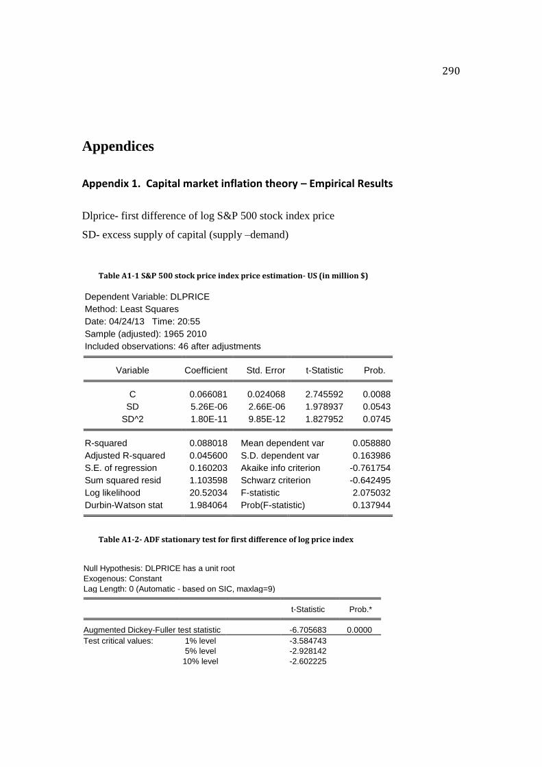
290
Appendices
Appendix 1. Capital market inflation theory – Empirical Results
Dlprice- first difference of log S&P 500 stock index price
SD- excess supply of capital (supply –demand)
Table A1-1 S&P 500 stock price index price estimation- US (in million $)
Dependent Variable: DLPRICE
Method: Least Squares
Date: 04/24/13 Time: 20:55
Sample (adjusted): 1965 2010
Included observations: 46 after adjustments
Variable Coefficient Std. Error t-Statistic Prob.
C 0.066081 0.024068 2.745592 0.0088
SD 5.26E-06 2.66E-06 1.978937 0.0543
SD^2 1.80E-11 9.85E-12 1.827952 0.0745
R-squared 0.088018 Mean dependent var 0.058880
Adjusted R-squared 0.045600 S.D. dependent var 0.163986
S.E. of regression 0.160203 Akaike info criterion -0.761754
Sum squared resid 1.103598 Schwarz criterion -0.642495
Log likelihood 20.52034 F-statistic 2.075032
Durbin-Watson stat 1.984064 Prob(F-statistic) 0.137944
Table A1-2- ADF stationary test for first difference of log price index
Null Hypothesis: DLPRICE has a unit root
Exogenous: Constant
Lag Length: 0 (Automatic - based on SIC, maxlag=9) t-Statistic Prob.* Augmented Dickey-Fuller test statistic -6.705683 0.0000
Test critical values: 1% level -3.584743
5% level -2.928142
10% level -2.602225
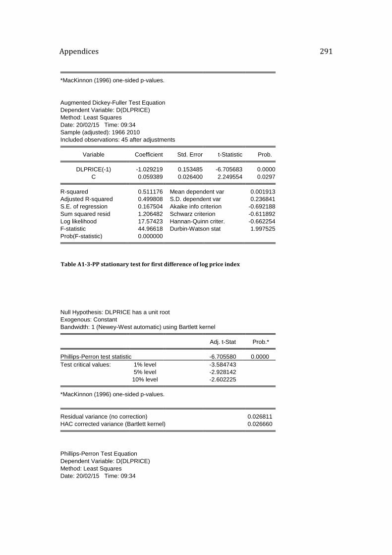
Appendices 291
*MacKinnon (1996) one-sided p-values.
Augmented Dickey-Fuller Test Equation
Dependent Variable: D(DLPRICE)
Method: Least Squares
Date: 20/02/15 Time: 09:34
Sample (adjusted): 1966 2010
Included observations: 45 after adjustments Variable Coefficient Std. Error t-Statistic Prob. DLPRICE(-1) -1.029219 0.153485 -6.705683 0.0000
C 0.059389 0.026400 2.249554 0.0297 R-squared 0.511176 Mean dependent var 0.001913
Adjusted R-squared 0.499808 S.D. dependent var 0.236841
S.E. of regression 0.167504 Akaike info criterion -0.692188
Sum squared resid 1.206482 Schwarz criterion -0.611892
Log likelihood 17.57423 Hannan-Quinn criter. -0.662254
F-statistic 44.96618 Durbin-Watson stat 1.997525
Prob(F-statistic) 0.000000
Table A1-3-PP stationary test for first difference of log price index
Null Hypothesis: DLPRICE has a unit root
Exogenous: Constant
Bandwidth: 1 (Newey-West automatic) using Bartlett kernel Adj. t-Stat Prob.* Phillips-Perron test statistic -6.705580 0.0000
Test critical values: 1% level -3.584743
5% level -2.928142
10% level -2.602225 *MacKinnon (1996) one-sided p-values.
Residual variance (no correction) 0.026811
HAC corrected variance (Bartlett kernel) 0.026660
Phillips-Perron Test Equation
Dependent Variable: D(DLPRICE)
Method: Least Squares
Date: 20/02/15 Time: 09:34

Appendices 292
Sample (adjusted): 1966 2010
Included observations: 45 after adjustments Variable Coefficient Std. Error t-Statistic Prob. DLPRICE(-1) -1.029219 0.153485 -6.705683 0.0000
C 0.059389 0.026400 2.249554 0.0297 R-squared 0.511176 Mean dependent var 0.001913
Adjusted R-squared 0.499808 S.D. dependent var 0.236841
S.E. of regression 0.167504 Akaike info criterion -0.692188
Sum squared resid 1.206482 Schwarz criterion -0.611892
Log likelihood 17.57423 Hannan-Quinn criter. -0.662254
F-statistic 44.96618 Durbin-Watson stat 1.997525
Prob(F-statistic) 0.000000
Table A1-4 KPSS stationary test for first difference of log price index
Null Hypothesis: DLPRICE is stationary
Exogenous: Constant
Bandwidth: 2 (Newey-West automatic) using Bartlett kernel LM-Stat. Kwiatkowski-Phillips-Schmidt-Shin test statistic 0.138124
Asymptotic critical values*: 1% level 0.739000
5% level 0.463000
10% level 0.347000 *Kwiatkowski-Phillips-Schmidt-Shin (1992, Table 1)
Residual variance (no correction) 0.026307
HAC corrected variance (Bartlett kernel) 0.022806
KPSS Test Equation
Dependent Variable: DLPRICE
Method: Least Squares
Date: 20/02/15 Time: 09:35
Sample (adjusted): 1965 2010
Included observations: 46 after adjustments Variable Coefficient Std. Error t-Statistic Prob. C 0.058880 0.024178 2.435236 0.0189 R-squared 0.000000 Mean dependent var 0.058880
Adjusted R-squared 0.000000 S.D. dependent var 0.163986
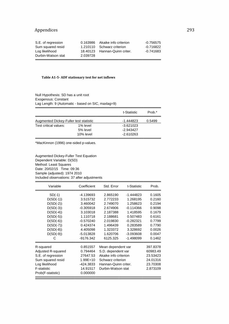
Appendices 293
S.E. of regression 0.163986 Akaike info criterion -0.756575
Sum squared resid 1.210110 Schwarz criterion -0.716822
Log likelihood 18.40123 Hannan-Quinn criter. -0.741683
Durbin-Watson stat 2.039728
Table A1-5- ADF stationary test for net inflows
Null Hypothesis: SD has a unit root
Exogenous: Constant
Lag Length: 9 (Automatic - based on SIC, maxlag=9) t-Statistic Prob.* Augmented Dickey-Fuller test statistic -1.444823 0.5499
Test critical values: 1% level -3.621023
5% level -2.943427
10% level -2.610263 *MacKinnon (1996) one-sided p-values.
Augmented Dickey-Fuller Test Equation
Dependent Variable: D(SD)
Method: Least Squares
Date: 20/02/15 Time: 09:36
Sample (adjusted): 1974 2010
Included observations: 37 after adjustments Variable Coefficient Std. Error t-Statistic Prob. SD(-1) -4.139693 2.865190 -1.444823 0.1605
D(SD(-1)) 3.515732 2.772233 1.268195 0.2160
D(SD(-2)) 3.460042 2.749070 1.258623 0.2194
D(SD(-3)) -0.305918 2.674906 -0.114366 0.9098
D(SD(-4)) 3.103018 2.187388 1.418595 0.1679
D(SD(-5)) 1.110718 2.188681 0.507483 0.6161
D(SD(-6)) -0.570240 2.019830 -0.282321 0.7799
D(SD(-7)) 0.424374 1.496439 0.283589 0.7790
D(SD(-8)) 4.405098 1.323372 3.328692 0.0026
D(SD(-9)) -5.013828 1.620706 -3.093608 0.0047
C -9176.342 6125.325 -1.498099 0.1462 R-squared 0.851557 Mean dependent var 397.8378
Adjusted R-squared 0.794464 S.D. dependent var 60983.49
S.E. of regression 27647.53 Akaike info criterion 23.53423
Sum squared resid 1.99E+10 Schwarz criterion 24.01316
Log likelihood -424.3833 Hannan-Quinn criter. 23.70308
F-statistic 14.91517 Durbin-Watson stat 2.873109
Prob(F-statistic) 0.000000
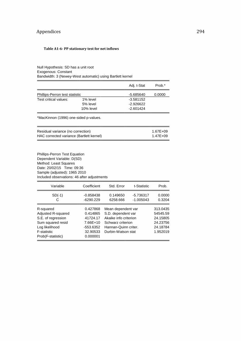
Appendices 294
Table A1-6- PP stationary test for net inflows
Null Hypothesis: SD has a unit root
Exogenous: Constant
Bandwidth: 3 (Newey-West automatic) using Bartlett kernel Adj. t-Stat Prob.* Phillips-Perron test statistic -5.685640 0.0000
Test critical values: 1% level -3.581152
5% level -2.926622
10% level -2.601424 *MacKinnon (1996) one-sided p-values.
Residual variance (no correction) 1.67E+09
HAC corrected variance (Bartlett kernel) 1.47E+09
Phillips-Perron Test Equation
Dependent Variable: D(SD)
Method: Least Squares
Date: 20/02/15 Time: 09:36
Sample (adjusted): 1965 2010
Included observations: 46 after adjustments Variable Coefficient Std. Error t-Statistic Prob. SD(-1) -0.858438 0.149650 -5.736317 0.0000
C -6290.229 6258.666 -1.005043 0.3204 R-squared 0.427868 Mean dependent var 313.0435
Adjusted R-squared 0.414865 S.D. dependent var 54545.59
S.E. of regression 41724.17 Akaike info criterion 24.15805
Sum squared resid 7.66E+10 Schwarz criterion 24.23756
Log likelihood -553.6352 Hannan-Quinn criter. 24.18784
F-statistic 32.90533 Durbin-Watson stat 1.952019
Prob(F-statistic) 0.000001

Appendices 295
Table A1-7- KPSS stationary test for net inflows
Null Hypothesis: SD is stationary
Exogenous: Constant
Bandwidth: 1 (Newey-West automatic) using Bartlett kernel LM-Stat. Kwiatkowski-Phillips-Schmidt-Shin test statistic 0.291585
Asymptotic critical values*: 1% level 0.739000
5% level 0.463000
10% level 0.347000 *Kwiatkowski-Phillips-Schmidt-Shin (1992, Table 1)
Residual variance (no correction) 1.66E+09
HAC corrected variance (Bartlett kernel) 1.90E+09
KPSS Test Equation
Dependent Variable: SD
Method: Least Squares
Date: 20/02/15 Time: 09:37
Sample: 1964 2010
Included observations: 47 Variable Coefficient Std. Error t-Statistic Prob. C -7224.362 6014.533 -1.201151 0.2358 R-squared 0.000000 Mean dependent var -7224.362
Adjusted R-squared 0.000000 S.D. dependent var 41233.56
S.E. of regression 41233.56 Akaike info criterion 24.11294
Sum squared resid 7.82E+10 Schwarz criterion 24.15230
Log likelihood -565.6541 Hannan-Quinn criter. 24.12775
Durbin-Watson stat 1.711934
Table A1-8 Granger causality – 2 lags
Pairwise Granger Causality Tests
Date: 09/22/14 Time: 12:38
Sample: 1964 2010
Lags: 2
Null Hypothesis: Obs F-Statistic Probability
DLPRICE does not Granger Cause SD 44 0.02556 0.97478
SD does not Granger Cause DLPRICE 5.04214 0.01128

Appendices 296
Table A1-9 Granger causality – 4 lags
Pairwise Granger Causality Tests
Date: 20/02/15 Time: 09:39
Sample: 1964 2010
Lags: 4 Null Hypothesis: Obs F-Statistic Prob. DLPRICE does not Granger Cause SD 42 0.32119 0.8617
SD does not Granger Cause DLPRICE 3.63288 0.0147
Table A1-10 Granger causality – 1 lag
Pairwise Granger Causality Tests
Date: 20/02/15 Time: 09:41
Sample: 1964 2010
Lags: 1 Null Hypothesis: Obs F-Statistic Prob. DLPRICE does not Granger Cause SD 45 0.34576 0.5597
SD does not Granger Cause DLPRICE 8.67153 0.0052
Table A1-11 Ramsey Reset Test
Ramsey RESET Test:
F-statistic 3.381462 Probability 0.043486
Log likelihood ratio 6.867831 Probability 0.032260
Test Equation:
Dependent Variable: DLPRICE
Method: Least Squares
Date: 04/25/13 Time: 00:27
Sample: 1965 2010
Included observations: 46
Variable Coefficient Std. Error t-Statistic Prob.
C 0.295721 0.309877 0.954318 0.3454
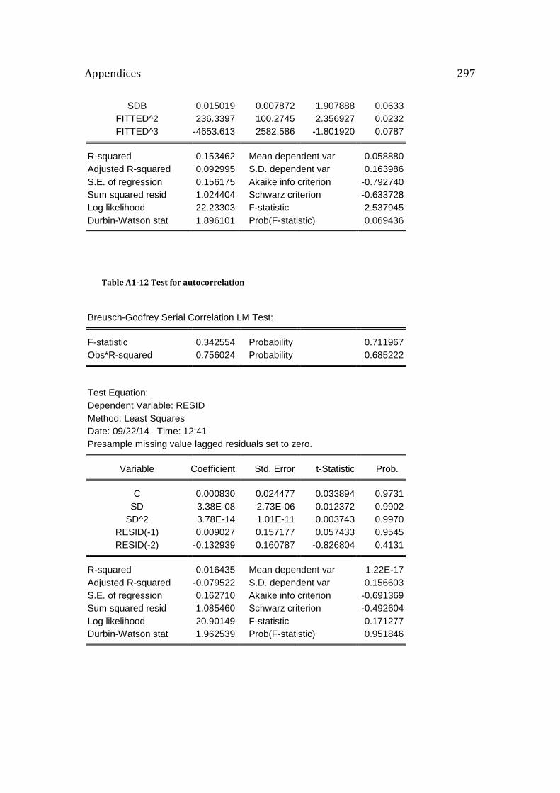
Appendices 297
SDB 0.015019 0.007872 1.907888 0.0633
FITTED^2 236.3397 100.2745 2.356927 0.0232
FITTED^3 -4653.613 2582.586 -1.801920 0.0787
R-squared 0.153462 Mean dependent var 0.058880
Adjusted R-squared 0.092995 S.D. dependent var 0.163986
S.E. of regression 0.156175 Akaike info criterion -0.792740
Sum squared resid 1.024404 Schwarz criterion -0.633728
Log likelihood 22.23303 F-statistic 2.537945
Durbin-Watson stat 1.896101 Prob(F-statistic) 0.069436
Table A1-12 Test for autocorrelation
Breusch-Godfrey Serial Correlation LM Test:
F-statistic 0.342554 Probability 0.711967
Obs*R-squared 0.756024 Probability 0.685222
Test Equation:
Dependent Variable: RESID
Method: Least Squares
Date: 09/22/14 Time: 12:41
Presample missing value lagged residuals set to zero.
Variable Coefficient Std. Error t-Statistic Prob.
C 0.000830 0.024477 0.033894 0.9731
SD 3.38E-08 2.73E-06 0.012372 0.9902
SD^2 3.78E-14 1.01E-11 0.003743 0.9970
RESID(-1) 0.009027 0.157177 0.057433 0.9545
RESID(-2) -0.132939 0.160787 -0.826804 0.4131
R-squared 0.016435 Mean dependent var 1.22E-17
Adjusted R-squared -0.079522 S.D. dependent var 0.156603
S.E. of regression 0.162710 Akaike info criterion -0.691369
Sum squared resid 1.085460 Schwarz criterion -0.492604
Log likelihood 20.90149 F-statistic 0.171277
Durbin-Watson stat 1.962539 Prob(F-statistic) 0.951846

Appendices 298
Table A1-13 Test for heteroskedasticity
White Heteroskedasticity Test:
F-statistic 1.278351 Probability 0.294183
Obs*R-squared 3.848855 Probability 0.278254
Test Equation:
Dependent Variable: RESID^2
Method: Least Squares
Date: 03/10/15 Time: 15:35
Sample: 1965 2010
Included observations: 46
Variable Coefficient Std. Error t-Statistic Prob.
C 0.021551 0.005709 3.775076 0.0005
SD 4.09E-07 7.61E-07 0.537107 0.5940
SD^2 3.68E-11 2.22E-11 1.662643 0.1038
(SD^2)^2 -4.67E-22 2.67E-22 -1.748873 0.0876
R-squared 0.083671 Mean dependent var 0.023991
Adjusted R-squared 0.018219 S.D. dependent var 0.037072
S.E. of regression 0.036733 Akaike info criterion -3.687363
Sum squared resid 0.056670 Schwarz criterion -3.528351
Log likelihood 88.80935 F-statistic 1.278351
Durbin-Watson stat 1.682079 Prob(F-statistic) 0.294183
Table A1-14 Test for normality of residuals

Appendices 299
Appendix 2 Capital market inflation theory- Empirical results for Japan
Table A2-1 Nikkei 225 stock price estimation
Dependent Variable: DLPRICE
Method: Least Squares
Date: 09/23/14 Time: 14:45
Sample (adjusted): 1981 2010
Included observations: 30 after adjustments
Variable Coefficient Std. Error t-Statistic Prob.
C 0.015858 0.052888 0.299841 0.7665
SUPPLY-DEMAND -1.41E-08 7.85E-07 -0.017902 0.9858
R-squared 0.000011 Mean dependent var 0.016405
Adjusted R-squared -0.035702 S.D. dependent var 0.232250
S.E. of regression 0.236360 Akaike info criterion 0.017415
Sum squared resid 1.564243 Schwarz criterion 0.110828
Log likelihood 1.738775 F-statistic 0.000320
Durbin-Watson stat 1.699425 Prob(F-statistic) 0.985844
0
2
4
6
8
10
12
-0.4 -0.2 -0.0 0.2
Series: Residuals
Sample 1965 2010
Observations 46
Mean 1.22e-17
Median 0.023549
Maximum 0.310716
Minimum -0.407596
Std. Dev. 0.156603
Skewness -0.695700
Kurtosis 3.335807
Jarque-Bera 3.926789
Probability 0.140381

Appendices 300
Table A2-2 Ramsey rest test
Ramsey RESET Test:
F-statistic 0.733431 Probability 0.489932
Log likelihood ratio 1.646511 Probability 0.439000
Test Equation:
Dependent Variable: DLPRICE
Method: Least Squares
Date: 09/23/14 Time: 14:43
Sample: 1981 2010
Included observations: 30
Variable Coefficient Std. Error t-Statistic Prob.
C -618.5187 591.3699 -1.045908 0.3052
SUPPLY-DEMAND 0.000840 0.000799 1.051217 0.3028
FITTED^2 3610679. 3467832. 1.041192 0.3074
FITTED^3 -72599398 70414989 -1.031022 0.3120
R-squared 0.053416 Mean dependent var 0.016405
Adjusted R-squared -0.055806 S.D. dependent var 0.232250
S.E. of regression 0.238642 Akaike info criterion 0.095865
Sum squared resid 1.480705 Schwarz criterion 0.282691
Log likelihood 2.562031 F-statistic 0.489059
Durbin-Watson stat 1.943978 Prob(F-statistic) 0.692889
Figure A2-3 Test of autocorrelation
Breusch-Godfrey Serial Correlation LM Test:
F-statistic 0.358482 Probability 0.702136
Obs*R-squared 0.805066 Probability 0.668624
Test Equation:
Dependent Variable: RESID
Method: Least Squares
Date: 03/10/15 Time: 15:40
Presample missing value lagged residuals set to zero.
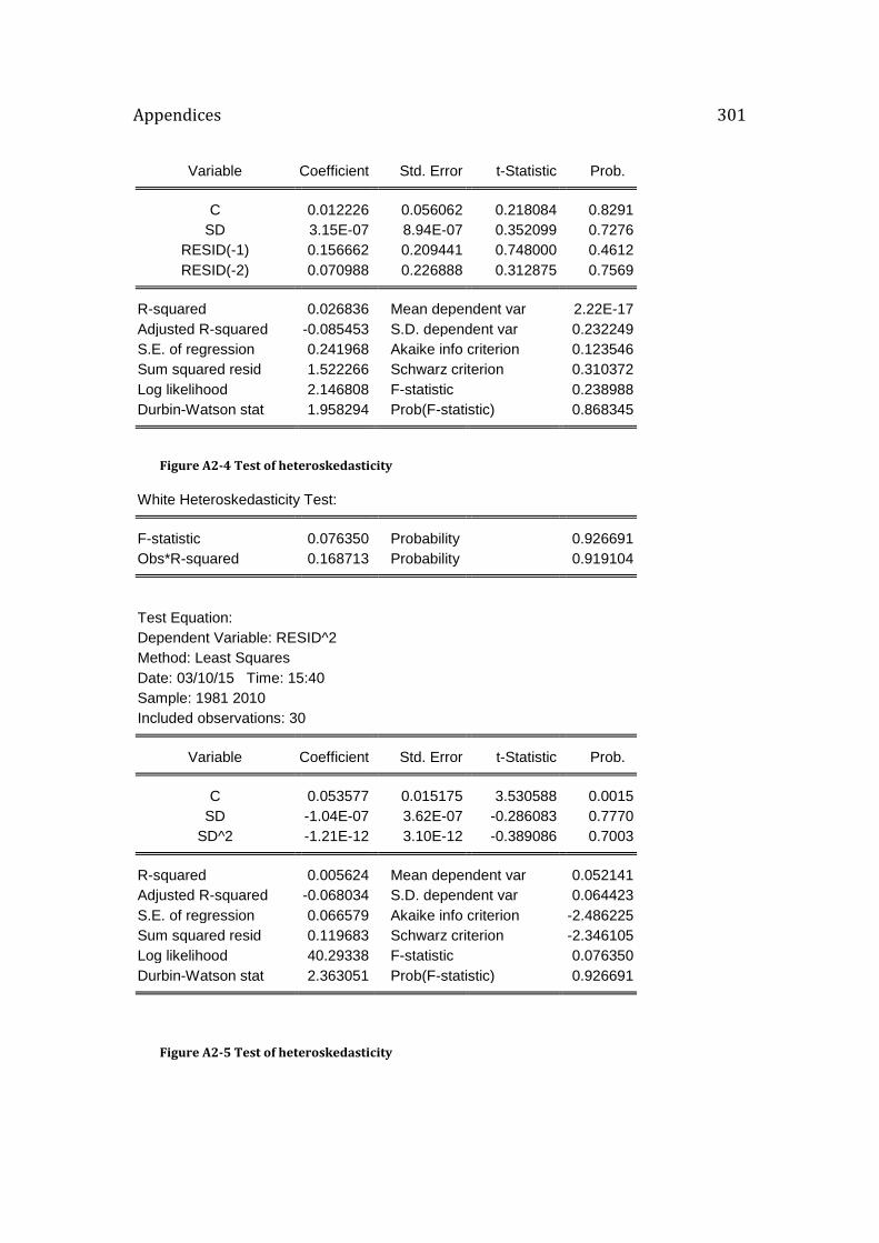
Appendices 301
Variable Coefficient Std. Error t-Statistic Prob.
C 0.012226 0.056062 0.218084 0.8291
SD 3.15E-07 8.94E-07 0.352099 0.7276
RESID(-1) 0.156662 0.209441 0.748000 0.4612
RESID(-2) 0.070988 0.226888 0.312875 0.7569
R-squared 0.026836 Mean dependent var 2.22E-17
Adjusted R-squared -0.085453 S.D. dependent var 0.232249
S.E. of regression 0.241968 Akaike info criterion 0.123546
Sum squared resid 1.522266 Schwarz criterion 0.310372
Log likelihood 2.146808 F-statistic 0.238988
Durbin-Watson stat 1.958294 Prob(F-statistic) 0.868345
Figure A2-4 Test of heteroskedasticity
White Heteroskedasticity Test:
F-statistic 0.076350 Probability 0.926691
Obs*R-squared 0.168713 Probability 0.919104
Test Equation:
Dependent Variable: RESID^2
Method: Least Squares
Date: 03/10/15 Time: 15:40
Sample: 1981 2010
Included observations: 30
Variable Coefficient Std. Error t-Statistic Prob.
C 0.053577 0.015175 3.530588 0.0015
SD -1.04E-07 3.62E-07 -0.286083 0.7770
SD^2 -1.21E-12 3.10E-12 -0.389086 0.7003
R-squared 0.005624 Mean dependent var 0.052141
Adjusted R-squared -0.068034 S.D. dependent var 0.064423
S.E. of regression 0.066579 Akaike info criterion -2.486225
Sum squared resid 0.119683 Schwarz criterion -2.346105
Log likelihood 40.29338 F-statistic 0.076350
Durbin-Watson stat 2.363051 Prob(F-statistic) 0.926691
Figure A2-5 Test of heteroskedasticity
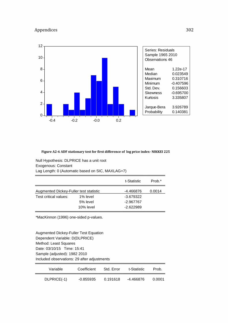
Appendices 302
Figure A2-6 ADF stationary test for first difference of log price index- NIKKEI 225
Null Hypothesis: DLPRICE has a unit root
Exogenous: Constant
Lag Length: 0 (Automatic based on SIC, MAXLAG=7) t-Statistic Prob.*
Augmented Dickey-Fuller test statistic -4.466876 0.0014
Test critical values: 1% level -3.679322
5% level -2.967767
10% level -2.622989
*MacKinnon (1996) one-sided p-values.
Augmented Dickey-Fuller Test Equation
Dependent Variable: D(DLPRICE)
Method: Least Squares
Date: 03/10/15 Time: 15:41
Sample (adjusted): 1982 2010
Included observations: 29 after adjustments
Variable Coefficient Std. Error t-Statistic Prob.
DLPRICE(-1) -0.855935 0.191618 -4.466876 0.0001
0
2
4
6
8
10
12
-0.4 -0.2 -0.0 0.2
Series: Residuals
Sample 1965 2010
Observations 46
Mean 1.22e-17
Median 0.023549
Maximum 0.310716
Minimum -0.407596
Std. Dev. 0.156603
Skewness -0.695700
Kurtosis 3.335807
Jarque-Bera 3.926789
Probability 0.140381

Appendices 303
C 0.012447 0.044220 0.281474 0.7805
R-squared 0.424957 Mean dependent var 0.002850
Adjusted R-squared 0.403659 S.D. dependent var 0.308008
S.E. of regression 0.237853 Akaike info criterion 0.032148
Sum squared resid 1.527505 Schwarz criterion 0.126444
Log likelihood 1.533856 F-statistic 19.95298
Durbin-Watson stat 1.981813 Prob(F-statistic) 0.000128
Figure A2-7 PP stationary test for first difference of log price index- NIKKEI 225
Null Hypothesis: DLPRICE has a unit root
Exogenous: Constant
Bandwidth: 4 (Newey-West using Bartlett kernel) Adj. t-Stat Prob.*
Phillips-Perron test statistic -4.418312 0.0016
Test critical values: 1% level -3.679322
5% level -2.967767
10% level -2.622989
*MacKinnon (1996) one-sided p-values.
Residual variance (no correction) 0.052673
HAC corrected variance (Bartlett kernel) 0.046284
Phillips-Perron Test Equation
Dependent Variable: D(DLPRICE)
Method: Least Squares
Date: 03/10/15 Time: 15:42
Sample (adjusted): 1982 2010
Included observations: 29 after adjustments
Variable Coefficient Std. Error t-Statistic Prob.
DLPRICE(-1) -0.855935 0.191618 -4.466876 0.0001
C 0.012447 0.044220 0.281474 0.7805
R-squared 0.424957 Mean dependent var 0.002850

Appendices 304
Adjusted R-squared 0.403659 S.D. dependent var 0.308008
S.E. of regression 0.237853 Akaike info criterion 0.032148
Sum squared resid 1.527505 Schwarz criterion 0.126444
Log likelihood 1.533856 F-statistic 19.95298
Durbin-Watson stat 1.981813 Prob(F-statistic) 0.000128
Figure A2-8 KPSS stationary test for first difference of log price index- NIKKEI 225
Null Hypothesis: DLPRICE is stationary
Exogenous: Constant
Bandwidth: 2 (Newey-West using Bartlett kernel) LM-Stat.
Kwiatkowski-Phillips-Schmidt-Shin test statistic 0.256698
Asymptotic critical values*: 1% level 0.739000
5% level 0.463000
10% level 0.347000
*Kwiatkowski-Phillips-Schmidt-Shin (1992, Table 1)
Residual variance (no correction) 0.052142
HAC corrected variance (Bartlett kernel) 0.064339
KPSS Test Equation
Dependent Variable: DLPRICE
Method: Least Squares
Date: 03/10/15 Time: 15:42
Sample (adjusted): 1981 2010
Included observations: 30 after adjustments
Variable Coefficient Std. Error t-Statistic Prob.
C 0.016405 0.042403 0.386895 0.7017
R-squared 0.000000 Mean dependent var 0.016405
Adjusted R-squared 0.000000 S.D. dependent var 0.232250
S.E. of regression 0.232250 Akaike info criterion -0.049240
Sum squared resid 1.564261 Schwarz criterion -0.002534
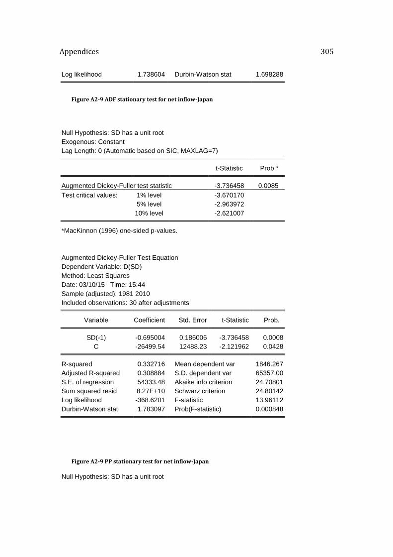
Appendices 305
Log likelihood 1.738604 Durbin-Watson stat 1.698288
Figure A2-9 ADF stationary test for net inflow-Japan
Null Hypothesis: SD has a unit root
Exogenous: Constant
Lag Length: 0 (Automatic based on SIC, MAXLAG=7) t-Statistic Prob.*
Augmented Dickey-Fuller test statistic -3.736458 0.0085
Test critical values: 1% level -3.670170
5% level -2.963972
10% level -2.621007
*MacKinnon (1996) one-sided p-values.
Augmented Dickey-Fuller Test Equation
Dependent Variable: D(SD)
Method: Least Squares
Date: 03/10/15 Time: 15:44
Sample (adjusted): 1981 2010
Included observations: 30 after adjustments
Variable Coefficient Std. Error t-Statistic Prob.
SD(-1) -0.695004 0.186006 -3.736458 0.0008
C -26499.54 12488.23 -2.121962 0.0428
R-squared 0.332716 Mean dependent var 1846.267
Adjusted R-squared 0.308884 S.D. dependent var 65357.00
S.E. of regression 54333.48 Akaike info criterion 24.70801
Sum squared resid 8.27E+10 Schwarz criterion 24.80142
Log likelihood -368.6201 F-statistic 13.96112
Durbin-Watson stat 1.783097 Prob(F-statistic) 0.000848
Figure A2-9 PP stationary test for net inflow-Japan
Null Hypothesis: SD has a unit root
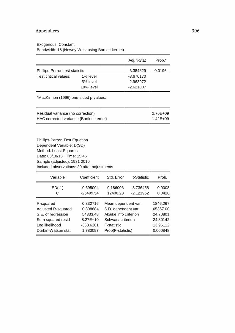
Appendices 306
Exogenous: Constant
Bandwidth: 16 (Newey-West using Bartlett kernel) Adj. t-Stat Prob.*
Phillips-Perron test statistic -3.384829 0.0196
Test critical values: 1% level -3.670170
5% level -2.963972
10% level -2.621007
*MacKinnon (1996) one-sided p-values.
Residual variance (no correction) 2.76E+09
HAC corrected variance (Bartlett kernel) 1.42E+09
Phillips-Perron Test Equation
Dependent Variable: D(SD)
Method: Least Squares
Date: 03/10/15 Time: 15:46
Sample (adjusted): 1981 2010
Included observations: 30 after adjustments
Variable Coefficient Std. Error t-Statistic Prob.
SD(-1) -0.695004 0.186006 -3.736458 0.0008
C -26499.54 12488.23 -2.121962 0.0428
R-squared 0.332716 Mean dependent var 1846.267
Adjusted R-squared 0.308884 S.D. dependent var 65357.00
S.E. of regression 54333.48 Akaike info criterion 24.70801
Sum squared resid 8.27E+10 Schwarz criterion 24.80142
Log likelihood -368.6201 F-statistic 13.96112
Durbin-Watson stat 1.783097 Prob(F-statistic) 0.000848
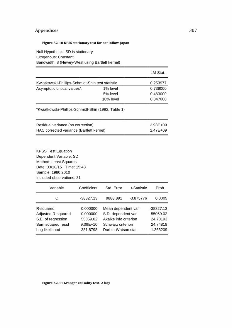
Appendices 307
Figure A2-10 KPSS stationary test for net inflow-Japan
Null Hypothesis: SD is stationary
Exogenous: Constant
Bandwidth: 8 (Newey-West using Bartlett kernel) LM-Stat.
Kwiatkowski-Phillips-Schmidt-Shin test statistic 0.253977
Asymptotic critical values*: 1% level 0.739000
5% level 0.463000
10% level 0.347000
*Kwiatkowski-Phillips-Schmidt-Shin (1992, Table 1)
Residual variance (no correction) 2.93E+09
HAC corrected variance (Bartlett kernel) 2.47E+09
KPSS Test Equation
Dependent Variable: SD
Method: Least Squares
Date: 03/10/15 Time: 15:43
Sample: 1980 2010
Included observations: 31
Variable Coefficient Std. Error t-Statistic Prob.
C -38327.13 9888.891 -3.875776 0.0005
R-squared 0.000000 Mean dependent var -38327.13
Adjusted R-squared 0.000000 S.D. dependent var 55059.02
S.E. of regression 55059.02 Akaike info criterion 24.70193
Sum squared resid 9.09E+10 Schwarz criterion 24.74818
Log likelihood -381.8798 Durbin-Watson stat 1.363209
Figure A2-11 Granger causality test- 2 lags
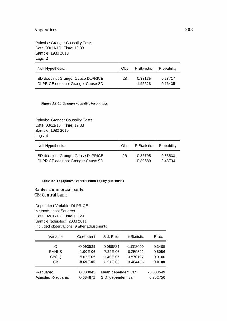
Appendices 308
Pairwise Granger Causality Tests
Date: 03/11/15 Time: 12:38
Sample: 1980 2010
Lags: 2
Null Hypothesis: Obs F-Statistic Probability
SD does not Granger Cause DLPRICE 28 0.38135 0.68717
DLPRICE does not Granger Cause SD 1.95528 0.16435
Figure A3-12 Granger causality test- 4 lags
Pairwise Granger Causality Tests
Date: 03/11/15 Time: 12:38
Sample: 1980 2010
Lags: 4
Null Hypothesis: Obs F-Statistic Probability
SD does not Granger Cause DLPRICE 26 0.32795 0.85533
DLPRICE does not Granger Cause SD 0.89689 0.48734
Table A2-13 Japanese central bank equity purchases
Banks: commercial banks CB: Central bank
Dependent Variable: DLPRICE
Method: Least Squares
Date: 02/10/13 Time: 03:29
Sample (adjusted): 2003 2011
Included observations: 9 after adjustments
Variable Coefficient Std. Error t-Statistic Prob.
C -0.093539 0.088831 -1.053000 0.3405
BANKS -1.90E-06 7.32E-06 -0.259521 0.8056
CB(-1) 5.02E-05 1.40E-05 3.570102 0.0160
CB -8.69E-05 2.51E-05 -3.464496 0.0180
R-squared 0.803045 Mean dependent var -0.003549
Adjusted R-squared 0.684872 S.D. dependent var 0.252750
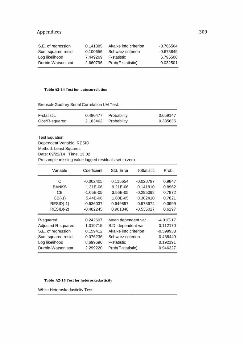
Appendices 309
S.E. of regression 0.141885 Akaike info criterion -0.766504
Sum squared resid 0.100656 Schwarz criterion -0.678849
Log likelihood 7.449269 F-statistic 6.795500
Durbin-Watson stat 2.660796 Prob(F-statistic) 0.032501
Table A2-14 Test for autocorrelation
Breusch-Godfrey Serial Correlation LM Test:
F-statistic 0.480477 Probability 0.659147
Obs*R-squared 2.183462 Probability 0.335635
Test Equation:
Dependent Variable: RESID
Method: Least Squares
Date: 09/22/14 Time: 13:02
Presample missing value lagged residuals set to zero.
Variable Coefficient Std. Error t-Statistic Prob.
C -0.002405 0.115654 -0.020797 0.9847
BANKS 1.31E-06 9.21E-06 0.141810 0.8962
CB -1.05E-05 3.56E-05 -0.295098 0.7872
CB(-1) 5.44E-06 1.80E-05 0.302410 0.7821
RESID(-1) -0.636037 0.649897 -0.978674 0.3999
RESID(-2) -0.482245 0.901348 -0.535027 0.6297
R-squared 0.242607 Mean dependent var -4.01E-17
Adjusted R-squared -1.019715 S.D. dependent var 0.112170
S.E. of regression 0.159412 Akaike info criterion -0.599933
Sum squared resid 0.076236 Schwarz criterion -0.468449
Log likelihood 8.699696 F-statistic 0.192191
Durbin-Watson stat 2.299220 Prob(F-statistic) 0.946327
Table A2-15 Test for heteroskedasticity
White Heteroskedasticity Test:
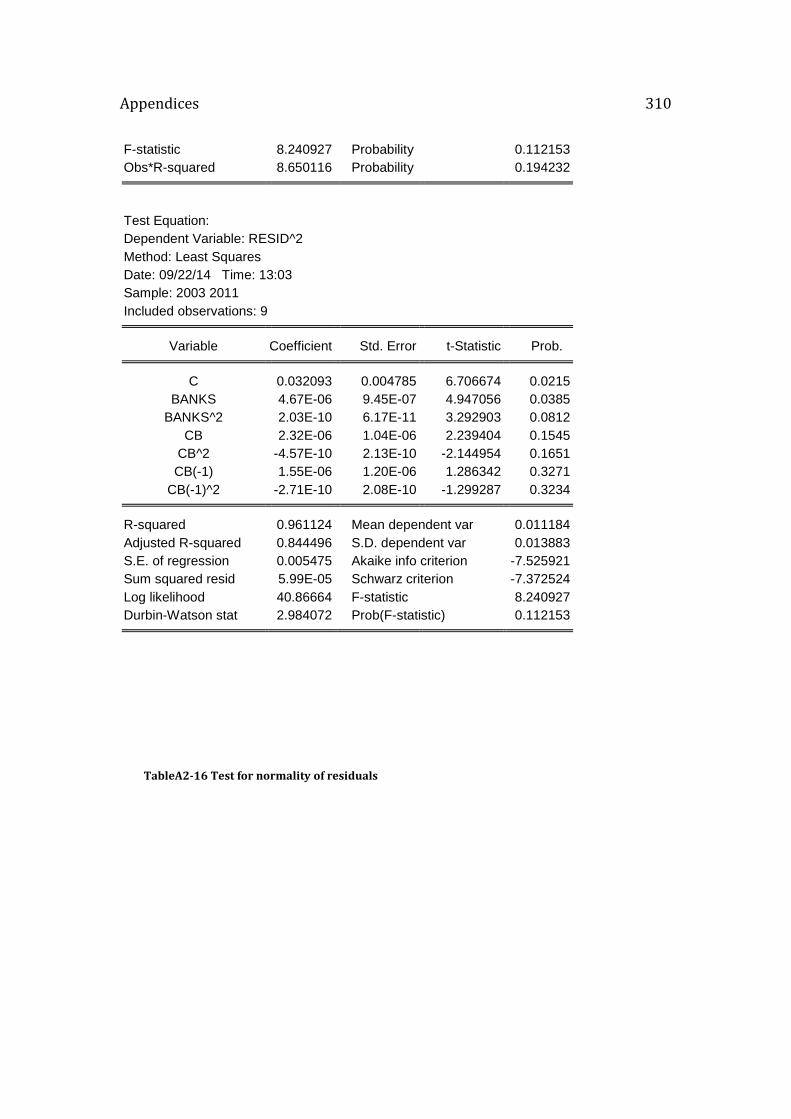
Appendices 310
F-statistic 8.240927 Probability 0.112153
Obs*R-squared 8.650116 Probability 0.194232
Test Equation:
Dependent Variable: RESID^2
Method: Least Squares
Date: 09/22/14 Time: 13:03
Sample: 2003 2011
Included observations: 9
Variable Coefficient Std. Error t-Statistic Prob.
C 0.032093 0.004785 6.706674 0.0215
BANKS 4.67E-06 9.45E-07 4.947056 0.0385
BANKS^2 2.03E-10 6.17E-11 3.292903 0.0812
CB 2.32E-06 1.04E-06 2.239404 0.1545
CB^2 -4.57E-10 2.13E-10 -2.144954 0.1651
CB(-1) 1.55E-06 1.20E-06 1.286342 0.3271
CB(-1)^2 -2.71E-10 2.08E-10 -1.299287 0.3234
R-squared 0.961124 Mean dependent var 0.011184
Adjusted R-squared 0.844496 S.D. dependent var 0.013883
S.E. of regression 0.005475 Akaike info criterion -7.525921
Sum squared resid 5.99E-05 Schwarz criterion -7.372524
Log likelihood 40.86664 F-statistic 8.240927
Durbin-Watson stat 2.984072 Prob(F-statistic) 0.112153
TableA2-16 Test for normality of residuals

Appendices 311
Appendix 3 Empirical results for U.S. simple logit model Tier- Tier I capital ratio D08- 2008 dummy variable D09- 2009 dummy variable Size- Bank size dummy variable
Table A3-1 Result of simple logit model
Table A3-2 Result of marginal effects, for simple logit model
0.0
0.4
0.8
1.2
1.6
2.0
2.4
-0.2 -0.1 -0.0 0.1 0.2
Series: Residuals
Sample 2003 2011
Observations 9
Mean -4.01e-17
Median -0.032941
Maximum 0.186411
Minimum -0.188073
Std. Dev. 0.112170
Skewness 0.054374
Kurtosis 2.369662
Jarque-Bera 0.153432
Probability 0.926153
.
_cons -4.044033 1.38124 -2.93 0.003 -6.751214 -1.336852 d09 1.840682 .9641751 1.91 0.056 -.0490664 3.730431 d08 2.127516 .9446655 2.25 0.024 .276006 3.979027 size -1.09822 .5367322 -2.05 0.041 -2.150195 -.0462437 tier .1657921 .0848963 1.95 0.051 -.0006016 .3321857 failure Coef. Std. Err. z P>|z| [95% Conf. Interval] Robust (Std. Err. adjusted for 38 clusters in id)
Log pseudolikelihood = -40.385233 Pseudo R2 = 0.1538 Prob > chi2 = 0.0196 Wald chi2(4) = 11.72Logistic regression Number of obs = 103
Iteration 4: log pseudolikelihood = -40.385233Iteration 3: log pseudolikelihood = -40.385355Iteration 2: log pseudolikelihood = -40.413974Iteration 1: log pseudolikelihood = -41.149972Iteration 0: log pseudolikelihood = -47.725037
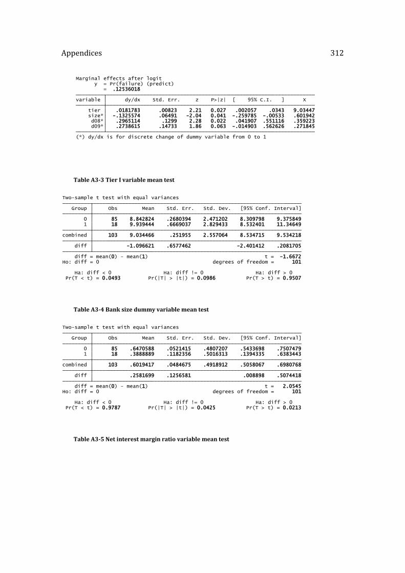
Appendices 312
Table A3-3 Tier I variable mean test
Table A3-4 Bank size dummy variable mean test
Table A3-5 Net interest margin ratio variable mean test
(*) dy/dx is for discrete change of dummy variable from 0 to 1 d09* .2738615 .14733 1.86 0.063 -.014903 .562626 .271845 d08* .2965114 .1299 2.28 0.022 .041907 .551116 .359223 size* -.1325574 .06491 -2.04 0.041 -.259785 -.00533 .601942 tier .0181783 .00823 2.21 0.027 .002057 .0343 9.03447 variable dy/dx Std. Err. z P>|z| [ 95% C.I. ] X = .12536018 y = Pr(failure) (predict)Marginal effects after logit
Pr(T < t) = 0.0493 Pr(|T| > |t|) = 0.0986 Pr(T > t) = 0.9507 Ha: diff < 0 Ha: diff != 0 Ha: diff > 0
Ho: diff = 0 degrees of freedom = 101 diff = mean(0) - mean(1) t = -1.6672 diff -1.096621 .6577462 -2.401412 .2081705 combined 103 9.034466 .251955 2.557064 8.534715 9.534218 1 18 9.939444 .6669037 2.829433 8.532401 11.34649 0 85 8.842824 .2680394 2.471202 8.309798 9.375849 Group Obs Mean Std. Err. Std. Dev. [95% Conf. Interval] Two-sample t test with equal variances
Pr(T < t) = 0.9787 Pr(|T| > |t|) = 0.0425 Pr(T > t) = 0.0213 Ha: diff < 0 Ha: diff != 0 Ha: diff > 0
Ho: diff = 0 degrees of freedom = 101 diff = mean(0) - mean(1) t = 2.0545 diff .2581699 .1256581 .008898 .5074418 combined 103 .6019417 .0484675 .4918912 .5058067 .6980768 1 18 .3888889 .1182356 .5016313 .1394335 .6383443 0 85 .6470588 .0521415 .4807207 .5433698 .7507479 Group Obs Mean Std. Err. Std. Dev. [95% Conf. Interval] Two-sample t test with equal variances
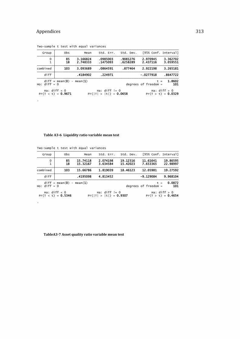
Appendices 313
Table A3-6 Liquidity ratio variable mean test
TableA3-7 Asset quality ratio variable mean test
.
Pr(T < t) = 0.9671 Pr(|T| > |t|) = 0.0658 Pr(T > t) = 0.0329 Ha: diff < 0 Ha: diff != 0 Ha: diff > 0
Ho: diff = 0 degrees of freedom = 101 diff = mean(0) - mean(1) t = 1.8602 diff .4184902 .224971 -.0277918 .8647722 combined 103 3.093689 .0864591 .877464 2.922198 3.265181 1 18 2.748333 .1475093 .6258289 2.437116 3.059551 0 85 3.166824 .0985003 .9081276 2.970945 3.362702 Group Obs Mean Std. Err. Std. Dev. [95% Conf. Interval] Two-sample t test with equal variances
.
Pr(T < t) = 0.5346 Pr(|T| > |t|) = 0.9307 Pr(T > t) = 0.4654 Ha: diff < 0 Ha: diff != 0 Ha: diff > 0
Ho: diff = 0 degrees of freedom = 101 diff = mean(0) - mean(1) t = 0.0872 diff .4195098 4.813452 -9.129084 9.968104 combined 103 15.66786 1.819039 18.46123 12.05981 19.27592 1 18 15.32167 3.634584 15.42023 7.653365 22.98997 0 85 15.74118 2.074198 19.12316 11.61641 19.86595 Group Obs Mean Std. Err. Std. Dev. [95% Conf. Interval] Two-sample t test with equal variances
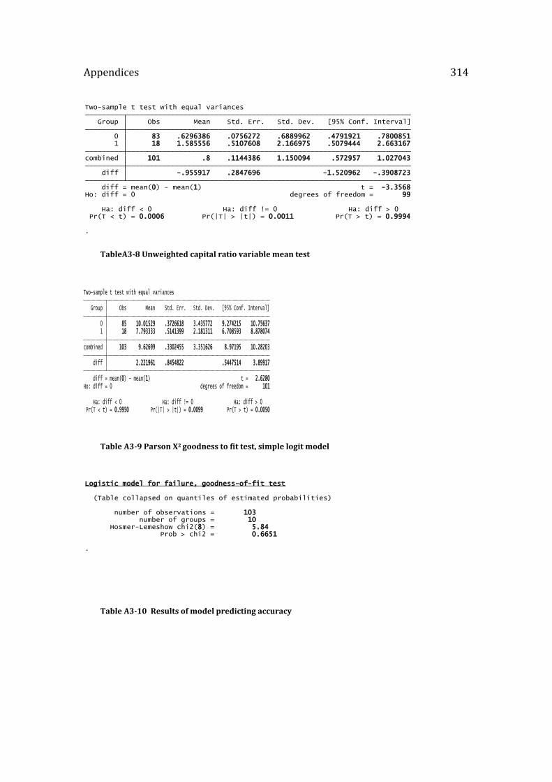
Appendices 314
TableA3-8 Unweighted capital ratio variable mean test
Table A3-9 Parson X2 goodness to fit test, simple logit model
Table A3-10 Results of model predicting accuracy
.
Pr(T < t) = 0.0006 Pr(|T| > |t|) = 0.0011 Pr(T > t) = 0.9994 Ha: diff < 0 Ha: diff != 0 Ha: diff > 0
Ho: diff = 0 degrees of freedom = 99 diff = mean(0) - mean(1) t = -3.3568 diff -.955917 .2847696 -1.520962 -.3908723 combined 101 .8 .1144386 1.150094 .572957 1.027043 1 18 1.585556 .5107608 2.166975 .5079444 2.663167 0 83 .6296386 .0756272 .6889962 .4791921 .7800851 Group Obs Mean Std. Err. Std. Dev. [95% Conf. Interval] Two-sample t test with equal variances
Pr(T < t) = 0.9950 Pr(|T| > |t|) = 0.0099 Pr(T > t) = 0.0050 Ha: diff < 0 Ha: diff != 0 Ha: diff > 0
Ho: diff = 0 degrees of freedom = 101 diff = mean(0) - mean(1) t = 2.6280 diff 2.221961 .8454822 .5447514 3.89917 combined 103 9.62699 .3302455 3.351626 8.97195 10.28203 1 18 7.793333 .5141399 2.181311 6.708593 8.878074 0 85 10.01529 .3726618 3.435772 9.274215 10.75637 Group Obs Mean Std. Err. Std. Dev. [95% Conf. Interval] Two-sample t test with equal variances
.
Prob > chi2 = 0.6651 Hosmer-Lemeshow chi2(8) = 5.84 number of groups = 10 number of observations = 103
(Table collapsed on quantiles of estimated probabilities)
Logistic model for failure, goodness-of-fit test
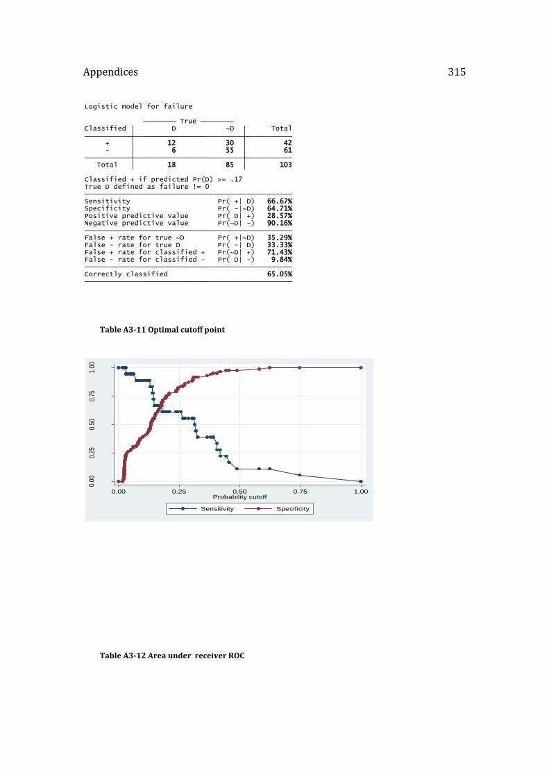
Appendices 315
Table A3-11 Optimal cutoff point
Table A3-12 Area under receiver ROC
Correctly classified 65.05% False - rate for classified - Pr( D| -) 9.84%False + rate for classified + Pr(~D| +) 71.43%False - rate for true D Pr( -| D) 33.33%False + rate for true ~D Pr( +|~D) 35.29% Negative predictive value Pr(~D| -) 90.16%Positive predictive value Pr( D| +) 28.57%Specificity Pr( -|~D) 64.71%Sensitivity Pr( +| D) 66.67% True D defined as failure != 0Classified + if predicted Pr(D) >= .17
Total 18 85 103 - 6 55 61 + 12 30 42 Classified D ~D Total True
Logistic model for failure
0.00
0.25
0.50
0.75
1.00
Sen
sitiv
ity/S
peci
ficity
0.00 0.25 0.50 0.75 1.00Probability cutoff
Sensitivity Specificity
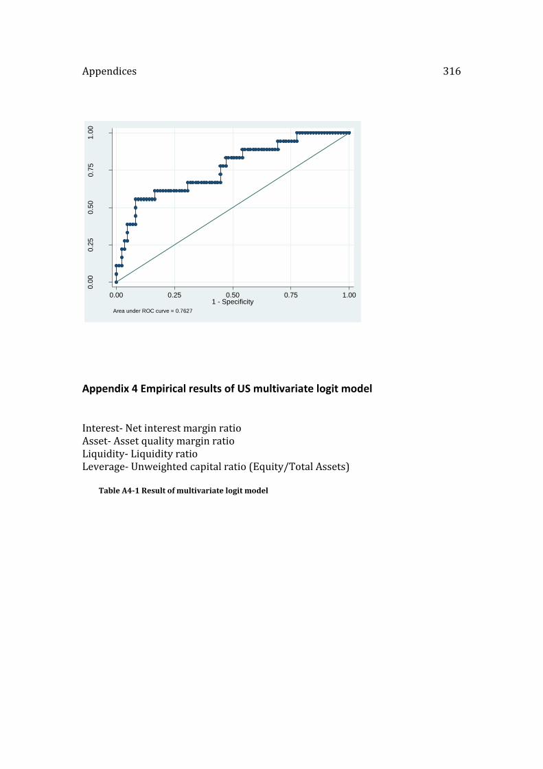
Appendices 316
Appendix 4 Empirical results of US multivariate logit model Interest- Net interest margin ratio Asset- Asset quality margin ratio Liquidity- Liquidity ratio Leverage- Unweighted capital ratio (Equity/Total Assets)
Table A4-1 Result of multivariate logit model
0.0
00.2
50.5
00.7
51.0
0
Sen
sitiv
ity
0.00 0.25 0.50 0.75 1.001 - Specificity
Area under ROC curve = 0.7627
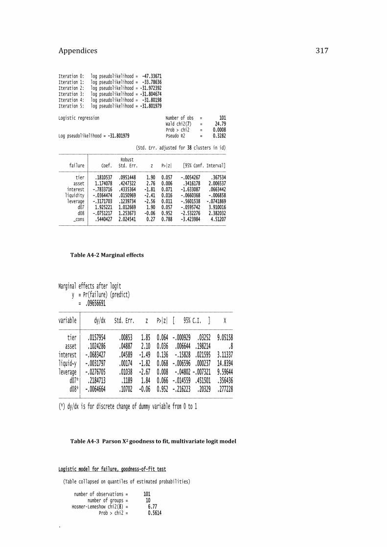
Appendices 317
Table A4-2 Marginal effects
Table A4-3 Parson X2 goodness to fit, multivariate logit model
_cons .5440427 2.024541 0.27 0.788 -3.423984 4.51207 d08 -.0751217 1.253673 -0.06 0.952 -2.532276 2.382032 d07 1.925221 1.012669 1.90 0.057 -.0595742 3.910016 leverage -.3171703 .1239734 -2.56 0.011 -.5601538 -.0741869 liquidity -.0364474 .0150969 -2.41 0.016 -.0660368 -.006858 interest -.7833716 .4335364 -1.81 0.071 -1.633087 .0663442 asset 1.174078 .4247322 2.76 0.006 .3416178 2.006537 tier .1810537 .0951448 1.90 0.057 -.0054267 .367534 failure Coef. Std. Err. z P>|z| [95% Conf. Interval] Robust (Std. Err. adjusted for 38 clusters in id)
Log pseudolikelihood = -31.801979 Pseudo R2 = 0.3282 Prob > chi2 = 0.0008 Wald chi2(7) = 24.79Logistic regression Number of obs = 101
Iteration 5: log pseudolikelihood = -31.801979Iteration 4: log pseudolikelihood = -31.80198Iteration 3: log pseudolikelihood = -31.804674Iteration 2: log pseudolikelihood = -31.972392Iteration 1: log pseudolikelihood = -33.78636Iteration 0: log pseudolikelihood = -47.33671
(*) dy/dx is for discrete change of dummy variable from 0 to 1 d08* -.0064664 .10702 -0.06 0.952 -.216223 .20329 .277228 d07* .2184713 .1189 1.84 0.066 -.014559 .451501 .356436leverage -.0276705 .01038 -2.67 0.008 -.04802 -.007321 9.59644liquid~y -.0031797 .00174 -1.82 0.068 -.006596 .000237 14.8394interest -.0683427 .04589 -1.49 0.136 -.15828 .021595 3.11337 asset .1024286 .04887 2.10 0.036 .006644 .198214 .8 tier .0157954 .00853 1.85 0.064 -.000929 .03252 9.05158 variable dy/dx Std. Err. z P>|z| [ 95% C.I. ] X = .09656691 y = Pr(failure) (predict)Marginal effects after logit
.
Prob > chi2 = 0.5614 Hosmer-Lemeshow chi2(8) = 6.77 number of groups = 10 number of observations = 101
(Table collapsed on quantiles of estimated probabilities)
Logistic model for failure, goodness-of-fit test
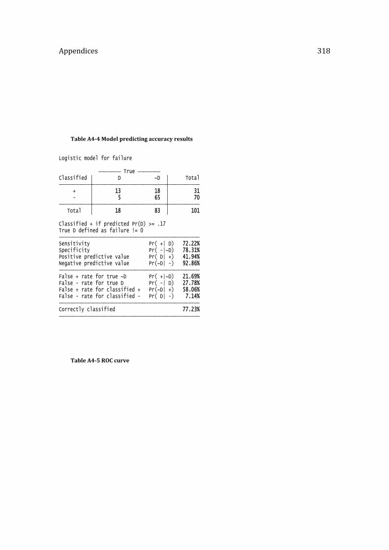
Appendices 318
Table A4-4 Model predicting accuracy results
Table A4-5 ROC curve
Correctly classified 77.23% False - rate for classified - Pr( D| -) 7.14%False + rate for classified + Pr(~D| +) 58.06%False - rate for true D Pr( -| D) 27.78%False + rate for true ~D Pr( +|~D) 21.69% Negative predictive value Pr(~D| -) 92.86%Positive predictive value Pr( D| +) 41.94%Specificity Pr( -|~D) 78.31%Sensitivity Pr( +| D) 72.22% True D defined as failure != 0Classified + if predicted Pr(D) >= .17
Total 18 83 101 - 5 65 70 + 13 18 31 Classified D ~D Total True
Logistic model for failure
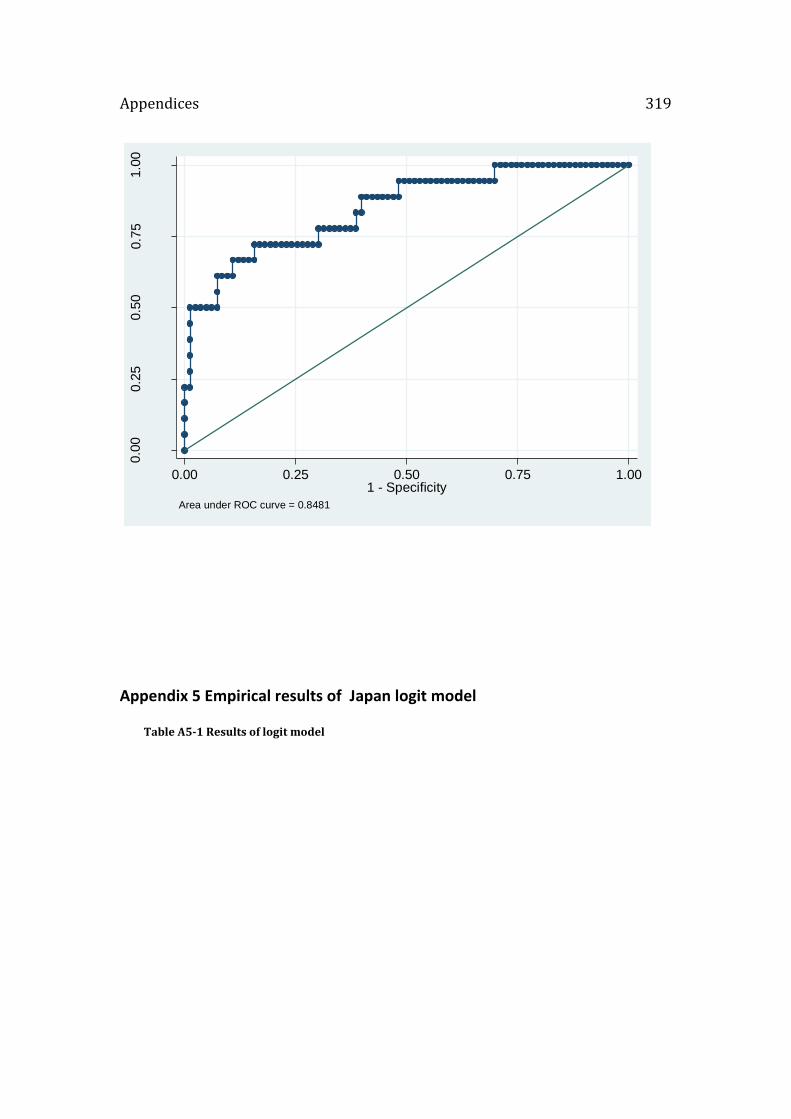
Appendices 319
Appendix 5 Empirical results of Japan logit model
Table A5-1 Results of logit model
0.0
00.2
50.5
00.7
51.0
0
Sen
sitiv
ity
0.00 0.25 0.50 0.75 1.001 - Specificity
Area under ROC curve = 0.8481
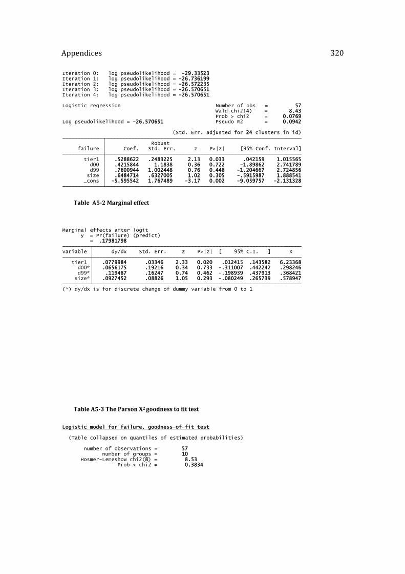
Appendices 320
Table A5-2 Marginal effect
Table A5-3 The Parson X2 goodness to fit test
_cons -5.595542 1.767489 -3.17 0.002 -9.059757 -2.131328 size .6484714 .6327005 1.02 0.305 -.5915987 1.888541 d99 .7600944 1.002448 0.76 0.448 -1.204667 2.724856 d00 .4215844 1.1838 0.36 0.722 -1.89862 2.741789 tier1 .5288622 .2483225 2.13 0.033 .042159 1.015565 failure Coef. Std. Err. z P>|z| [95% Conf. Interval] Robust (Std. Err. adjusted for 24 clusters in id)
Log pseudolikelihood = -26.570651 Pseudo R2 = 0.0942 Prob > chi2 = 0.0769 Wald chi2(4) = 8.43Logistic regression Number of obs = 57
Iteration 4: log pseudolikelihood = -26.570651Iteration 3: log pseudolikelihood = -26.570651Iteration 2: log pseudolikelihood = -26.572235Iteration 1: log pseudolikelihood = -26.736199Iteration 0: log pseudolikelihood = -29.33523
(*) dy/dx is for discrete change of dummy variable from 0 to 1 size* .0927452 .08826 1.05 0.293 -.080249 .265739 .578947 d99* .119487 .16247 0.74 0.462 -.198939 .437913 .368421 d00* .0656175 .19216 0.34 0.733 -.311007 .442242 .298246 tier1 .0779984 .03346 2.33 0.020 .012415 .143582 6.23368 variable dy/dx Std. Err. z P>|z| [ 95% C.I. ] X = .17981798 y = Pr(failure) (predict)Marginal effects after logit
Prob > chi2 = 0.3834 Hosmer-Lemeshow chi2(8) = 8.53 number of groups = 10 number of observations = 57
(Table collapsed on quantiles of estimated probabilities)
Logistic model for failure, goodness-of-fit test

Appendices 321
Table A5-4 Tier I variable mean test
Table A5-5 Bank size dummy variable mean test
Table A5-6 Optimal cutoff point
Pr(T < t) = 0.0280 Pr(|T| > |t|) = 0.0560 Pr(T > t) = 0.9720 Ha: diff < 0 Ha: diff != 0 Ha: diff > 0
Ho: diff = 0 degrees of freedom = 55 diff = mean(0) - mean(1) t = -1.9524 diff -.9031111 .462562 -1.830106 .0238839 combined 57 6.233684 .1932549 1.459043 5.846548 6.62082 1 12 6.946667 .3672138 1.272066 6.138434 7.754899 0 45 6.043556 .2175235 1.459192 5.605166 6.481945 Group Obs Mean Std. Err. Std. Dev. [95% Conf. Interval] Two-sample t test with equal variances
Pr(T < t) = 0.4865 Pr(|T| > |t|) = 0.9730 Pr(T > t) = 0.5135 Ha: diff < 0 Ha: diff != 0 Ha: diff > 0
Ho: diff = 0 degrees of freedom = 55 diff = mean(0) - mean(1) t = -0.0340 diff -.0055556 .1632976 -.3328113 .3217001 combined 57 .5789474 .0659772 .4981168 .4467792 .7111155 1 12 .5833333 .1486471 .5149287 .2561633 .9105034 0 45 .5777778 .0744603 .4994947 .427713 .7278426 Group Obs Mean Std. Err. Std. Dev. [95% Conf. Interval] Two-sample t test with equal variances
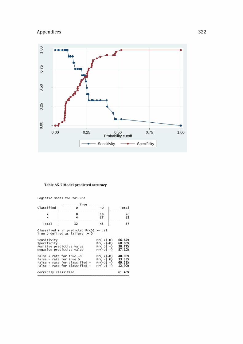
Appendices 322
Table A5-7 Model predicted accuracy
0.0
00.2
50.5
00.7
51.0
0
Sen
sitiv
ity/S
pe
cific
ity
0.00 0.25 0.50 0.75 1.00Probability cutoff
Sensitivity Specificity
Correctly classified 61.40% False - rate for classified - Pr( D| -) 12.90%False + rate for classified + Pr(~D| +) 69.23%False - rate for true D Pr( -| D) 33.33%False + rate for true ~D Pr( +|~D) 40.00% Negative predictive value Pr(~D| -) 87.10%Positive predictive value Pr( D| +) 30.77%Specificity Pr( -|~D) 60.00%Sensitivity Pr( +| D) 66.67% True D defined as failure != 0Classified + if predicted Pr(D) >= .21
Total 12 45 57 - 4 27 31 + 8 18 26 Classified D ~D Total True
Logistic model for failure
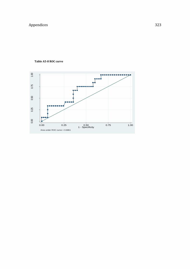
Appendices 323
Table A5-8 ROC curve
0.00
0.25
0.50
0.75
1.00
Sen
sitiv
ity
0.00 0.25 0.50 0.75 1.001 - Specificity
Area under ROC curve = 0.6861