For Online Publication Only APPENDIX: It’s Raining Men ...p3.storage.canalblog.com/32/34/1099015/113460587.pdf · 1 For Online Publication Only APPENDIX: It’s Raining Men! Hallelujah?

1

For Online Publication Only

APPENDIX: It’s Raining Men! Hallelujah?

Pauline Grosjean and Rose Khattar

Contents:

1. Additional Tables and Figures

2. Data Appendix

1. ADDITIONAL TABLES

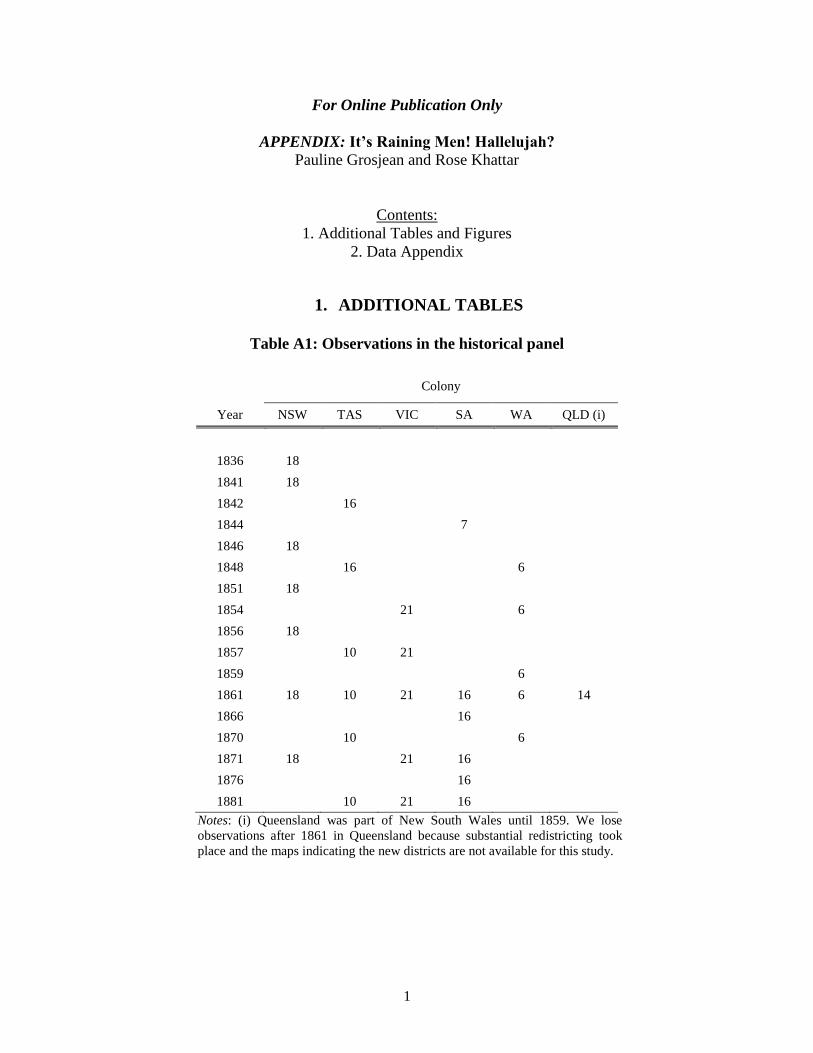
Table A1: Observations in the historical panel

Colony

Year NSW TAS VIC SA WA QLD (i)

1836 18

1841 18

1842 16

1844 7

1846 18

1848 16 6

1851 18

1854 21 6

1856 18

1857 10 21

1859 6

1861 18 10 21 16 6 14

1866 16

1870 10 6

1871 18 21 16

1876 16

1881 10 21 16

Notes: (i) Queensland was part of New South Wales until 1859. We lose

observations after 1861 in Queensland because substantial redistricting took

place and the maps indicating the new districts are not available for this study.

2

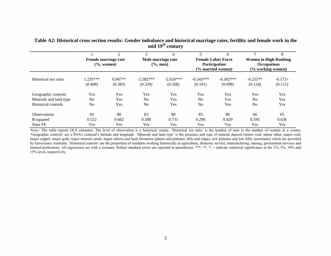
Table A2: Historical cross section results: Gender imbalance and historical marriage rates, fertility and female work in the

mid 19th

century

1 2 3 4 5 6 7 8

Female marriage rate

(%, women)

Male marriage rate

(%, men)

Female Labor Force

Participation

(% married women)

Women in High-Ranking

Occupations

(% working women)

Historical sex ratio 1.235*** 0.947** -2.382*** -2.024*** -0.343*** -0.302*** -0.255** -0.172+

(0.408) (0.383) (0.339) (0.268) (0.101) (0.098) (0.124) (0.111)

Geographic controls Yes Yes Yes Yes Yes Yes Yes Yes

Minerals and land type No Yes No Yes No Yes No Yes

Historical controls No Yes No Yes No Yes No Yes

Observations 83 80 83 80 83 80 66 65

R-squared 0.522 0.662 0.588 0.731 0.296 0.429 0.595 0.636

State FE Yes Yes Yes Yes Yes Yes Yes Yes

Notes: The table reports OLS estimates. The level of observation is a historical county. ‘Historical sex ratio’ is the number of men to the number of women in a county.

‘Geographic controls’ are a POA’s centroid’s latitude and longitude. ‘Minerals and land type’ is the presence and type of mineral deposit (minor coal; minor other; major coal;

major copper; major gold; major mineral sands; major others) and land formation (plains and plateaus; hills and ridges; low plateaus and low hills; mountains) which are provided

by Geoscience Australia. ‘Historical controls’ are the proportion of residents working historically in agriculture, domestic service, manufacturing, mining, government services and

learned professions. All regressions are with a constant. Robust standard errors are reported in parentheses. ***, **, *, + indicate statistical significance at the 1%, 5%, 10% and

15% level, respectively.

3

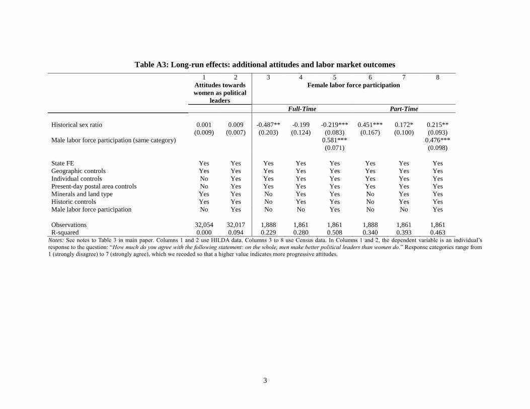
Table A3: Long-run effects: additional attitudes and labor market outcomes

1 2 3 4 5 6 7 8

Attitudes towards

women as political

leaders

Female labor force participation

Full-Time Part-Time

Historical sex ratio 0.001 0.009 -0.487** -0.199 -0.219*** 0.451*** 0.172* 0.215**

(0.009) (0.007) (0.203) (0.124) (0.083) (0.167) (0.100) (0.093)

Male labor force participation (same category) 0.581*** 0.476***

(0.071) (0.098)



Individual controls No Yes Yes Yes Yes Yes Yes Yes

Present-day postal area controls No Yes Yes Yes Yes Yes Yes Yes

Minerals and land type Yes Yes No Yes Yes No Yes Yes

Historic controls Yes Yes No Yes Yes No Yes Yes

Male labor force participation No Yes No No Yes No No Yes

Observations 32,054 32,017 1,888 1,861 1,861 1,888 1,861 1,861

R-squared 0.000 0.094 0.229 0.280 0.508 0.340 0.393 0.463 Notes: See notes to Table 3 in main paper. Columns 1 and 2 use HILDA data. Columns 3 to 8 use Census data. In Columns 1 and 2, the dependent variable is an individual’s

response to the question: “How much do you agree with the following statement: on the whole, men make better political leaders than women do.” Response categories range from

1 (strongly disagree) to 7 (strongly agree), which we recoded so that a higher value indicates more progressive attitudes.

4

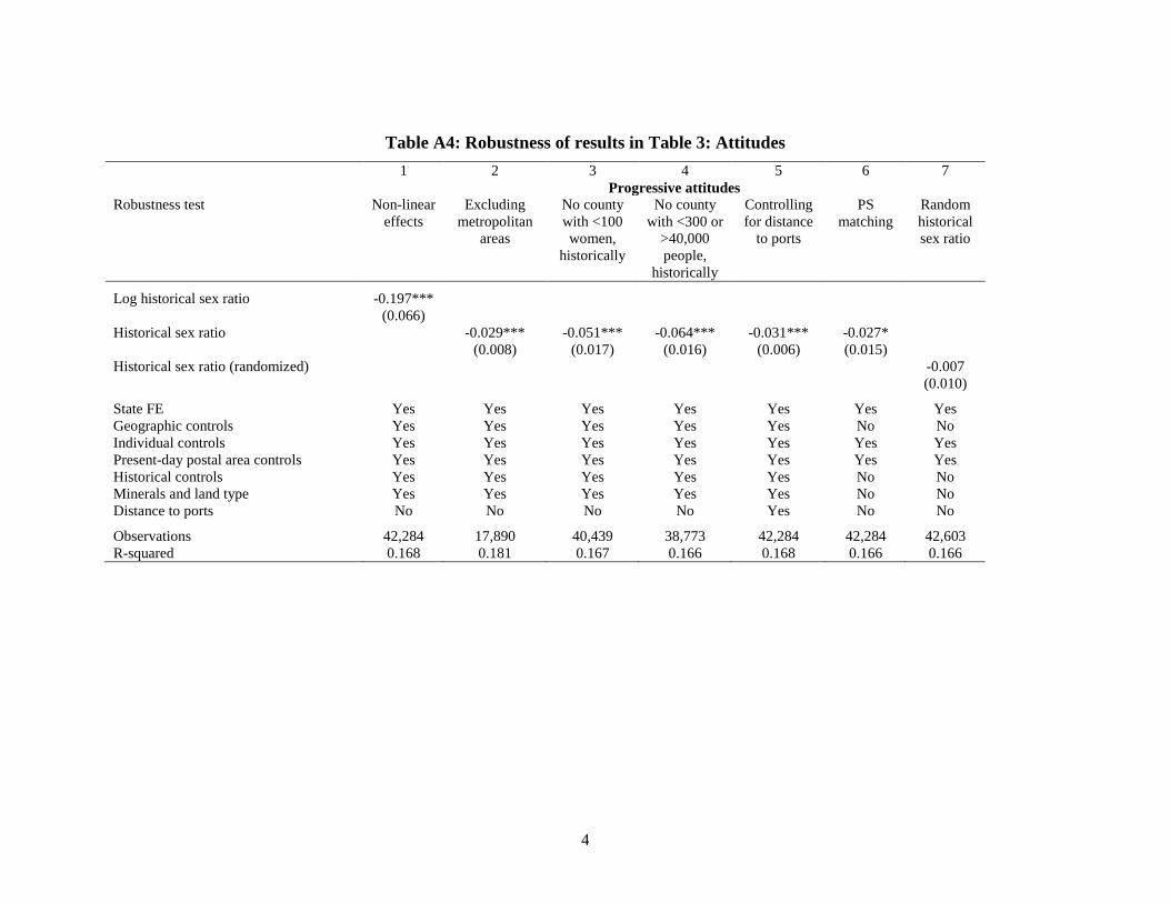
Table A4: Robustness of results in Table 3: Attitudes

1 2 3 4 5 6 7

Progressive attitudes

Robustness test Non-linear

effects

Excluding

metropolitan

areas

No county

with <100

women,

historically

No county

with <300 or

>40,000

people,

historically

Controlling

for distance

to ports

PS

matching

Random

historical

sex ratio

Log historical sex ratio -0.197***

(0.066)

Historical sex ratio -0.029*** -0.051*** -0.064*** -0.031*** -0.027*

(0.008) (0.017) (0.016) (0.006) (0.015)

Historical sex ratio (randomized) -0.007

(0.010)

State FE Yes Yes Yes Yes Yes Yes Yes

Geographic controls Yes Yes Yes Yes Yes No No

Individual controls Yes Yes Yes Yes Yes Yes Yes

Present-day postal area controls Yes Yes Yes Yes Yes Yes Yes

Historical controls Yes Yes Yes Yes Yes No No

Minerals and land type Yes Yes Yes Yes Yes No No

Distance to ports No No No No Yes No No

Observations 42,284 17,890 40,439 38,773 42,284 42,284 42,603

R-squared 0.168 0.181 0.167 0.166 0.168 0.166 0.166

5

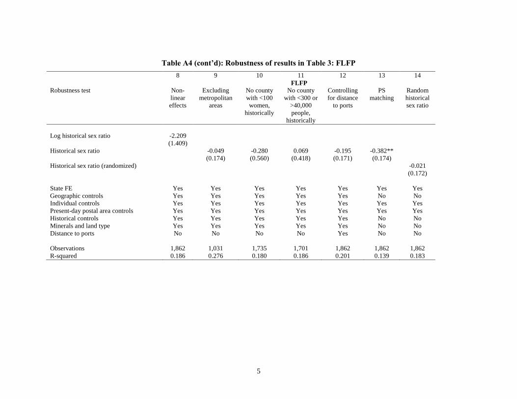
Table A4 (cont’d): Robustness of results in Table 3: FLFP

8 9 10 11 12 13 14

FLFP

Robustness test Non-

linear

effects

Excluding

metropolitan

areas

No county

with <100

women,

historically

No county

with <300 or

>40,000

people,

historically

Controlling

for distance

to ports

PS

matching

Random

historical

sex ratio

Log historical sex ratio -2.209

(1.409)

Historical sex ratio -0.049 -0.280 0.069 -0.195 -0.382**

(0.174) (0.560) (0.418) (0.171) (0.174)


(0.172)


Geographic controls Yes Yes Yes Yes Yes No No



Historical controls Yes Yes Yes Yes Yes No No

Minerals and land type Yes Yes Yes Yes Yes No No


Observations 1,862 1,031 1,735 1,701 1,862 1,862 1,862

R-squared 0.186 0.276 0.180 0.186 0.201 0.139 0.183

6

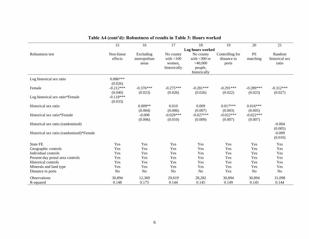
Table A4 (cont’d): Robustness of results in Table 3: Hours worked

15 16 17 18 19 20 21

Log hours worked


effects

Excluding

metropolitan

areas

No county

with <100

women,

historically

No county

with <300 or

>40,000

people,

historically

Controlling for

distance to

ports

PS

matching

Random

historical sex

ratio

Log historical sex ratio 0.086***

(0.026)

Female -0.212*** -0.376*** -0.275*** -0.281*** -0.291*** -0.289*** -0.312***

(0.040) (0.023) (0.026) (0.026) (0.022) (0.023) (0.027)

Log historical sex ratio*Female -0.118***

(0.033)

Historical sex ratio 0.009** 0.010 0.009 0.017*** 0.016***

(0.004) (0.006) (0.007) (0.003) (0.005)

Historical sex ratio*Female -0.008 -0.029*** -0.027*** -0.022*** -0.022***

(0.006) (0.010) (0.009) (0.007) (0.007)


(0.005)

Historical sex ratio (randomized)*Female -0.009

(0.010)


Geographic controls Yes Yes Yes Yes Yes Yes Yes



Historical controls Yes Yes Yes Yes Yes Yes Yes

Minerals and land type Yes Yes Yes Yes Yes Yes Yes


Observations 30,894 12,369 29,619 28,282 30,894 30,894 31,098

R-squared 0.148 0.175 0.144 0.145 0.149 0.145 0.144

7

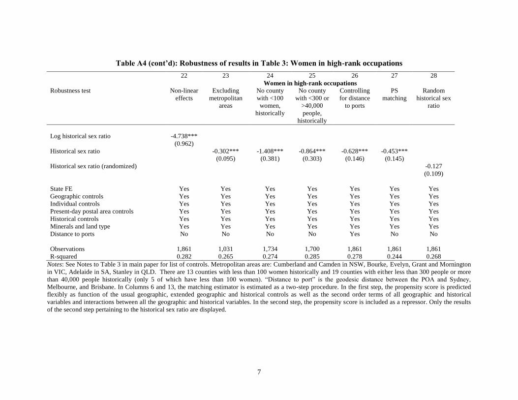
Table A4 (cont’d): Robustness of results in Table 3: Women in high-rank occupations

22 23 24 25 26 27 28

Women in high-rank occupations


effects

Excluding

metropolitan

areas

No county

with <100

women,

historically

No county

with <300 or

>40,000

people,

historically

Controlling

for distance

to ports

PS

matching

Random

historical sex

ratio

Log historical sex ratio -4.738***

(0.962)

Historical sex ratio -0.302*** -1.408*** -0.864*** -0.628*** -0.453***

(0.095) (0.381) (0.303) (0.146) (0.145)


(0.109)


Geographic controls Yes Yes Yes Yes Yes Yes Yes



Historical controls Yes Yes Yes Yes Yes Yes Yes

Minerals and land type Yes Yes Yes Yes Yes Yes Yes


Observations 1,861 1,031 1,734 1,700 1,861 1,861 1,861

R-squared 0.282 0.265 0.274 0.285 0.278 0.244 0.268

Notes: See Notes to Table 3 in main paper for list of controls. Metropolitan areas are: Cumberland and Camden in NSW, Bourke, Evelyn, Grant and Mornington

in VIC, Adelaide in SA, Stanley in QLD. There are 13 counties with less than 100 women historically and 19 counties with either less than 300 people or more

than 40,000 people historically (only 5 of which have less than 100 women). “Distance to port” is the geodesic distance between the POA and Sydney,

Melbourne, and Brisbane. In Columns 6 and 13, the matching estimator is estimated as a two-step procedure. In the first step, the propensity score is predicted

flexibly as function of the usual geographic, extended geographic and historical controls as well as the second order terms of all geographic and historical

variables and interactions between all the geographic and historical variables. In the second step, the propensity score is included as a repressor. Only the results

of the second step pertaining to the historical sex ratio are displayed.

8

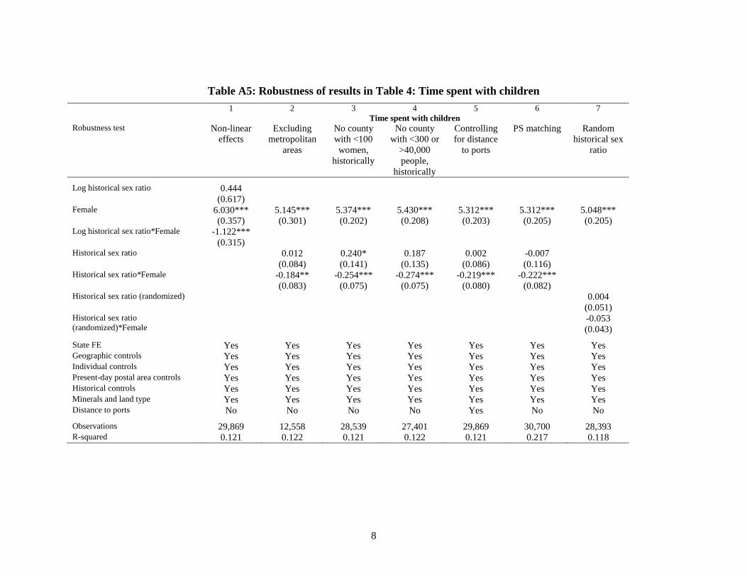
Table A5: Robustness of results in Table 4: Time spent with children

1 2 3 4 5 6 7

Time spent with children


effects

Excluding

metropolitan

areas

No county

with <100

women,

historically

No county

with <300 or

>40,000

people,

historically

Controlling

for distance

to ports

PS matching Random

historical sex

ratio

Log historical sex ratio 0.444 (0.617) Female 6.030*** 5.145*** 5.374*** 5.430*** 5.312*** 5.312*** 5.048*** (0.357) (0.301) (0.202) (0.208) (0.203) (0.205) (0.205) Log historical sex ratio*Female -1.122*** (0.315) Historical sex ratio 0.012 0.240* 0.187 0.002 -0.007 (0.084) (0.141) (0.135) (0.086) (0.116) Historical sex ratio*Female -0.184** -0.254*** -0.274*** -0.219*** -0.222*** (0.083) (0.075) (0.075) (0.080) (0.082) Historical sex ratio (randomized) 0.004

(0.051) Historical sex ratio

(randomized)*Female -0.053

(0.043) State FE Yes Yes Yes Yes Yes Yes Yes Geographic controls Yes Yes Yes Yes Yes Yes Yes Individual controls Yes Yes Yes Yes Yes Yes Yes Present-day postal area controls Yes Yes Yes Yes Yes Yes Yes Historical controls Yes Yes Yes Yes Yes Yes Yes Minerals and land type Yes Yes Yes Yes Yes Yes Yes Distance to ports No No No No Yes No No Observations 29,869 12,558 28,539 27,401 29,869 30,700 28,393 R-squared 0.121 0.122 0.121 0.122 0.121 0.217 0.118

9

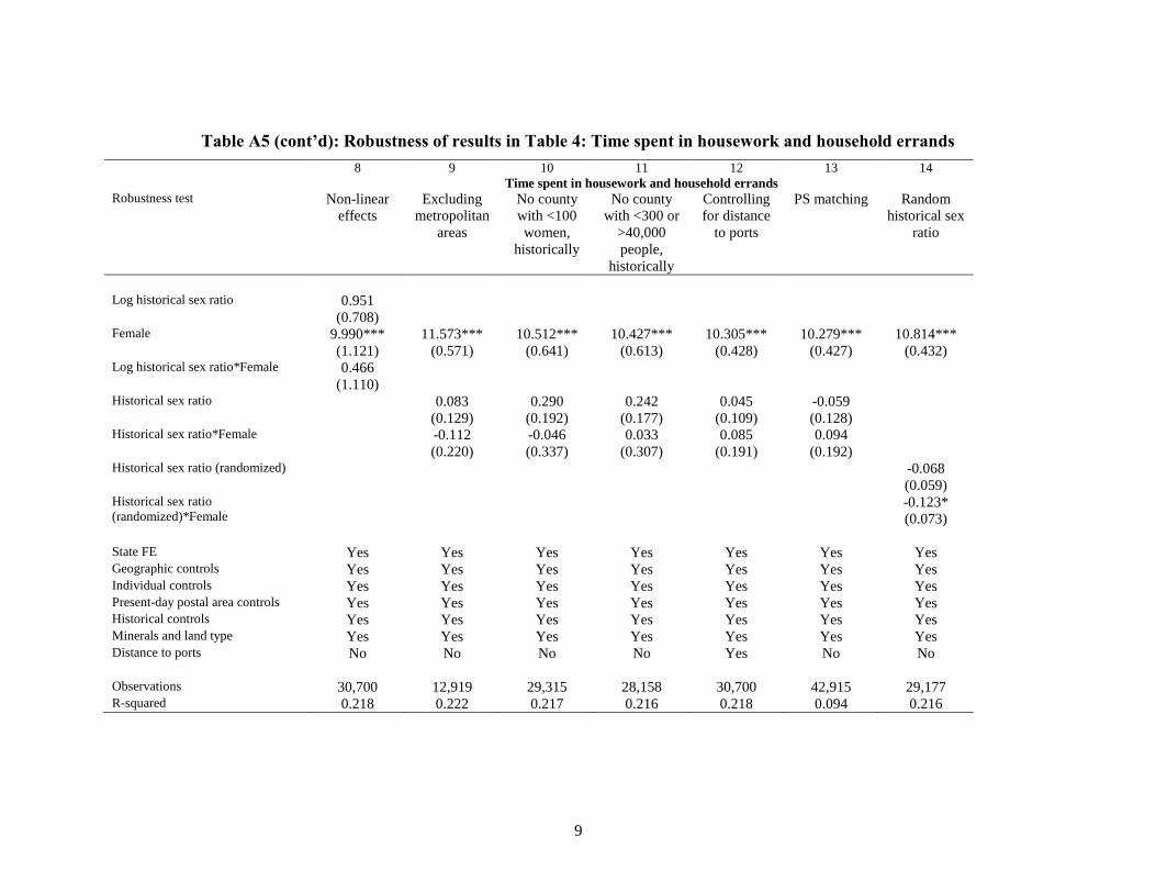
Table A5 (cont’d): Robustness of results in Table 4: Time spent in housework and household errands

8 9 10 11 12 13 14

Time spent in housework and household errands


effects

Excluding

metropolitan

areas

No county

with <100

women,

historically

No county

with <300 or

>40,000

people,

historically

Controlling

for distance

to ports

PS matching Random

historical sex

ratio

Log historical sex ratio 0.951 (0.708) Female 9.990*** 11.573*** 10.512*** 10.427*** 10.305*** 10.279*** 10.814*** (1.121) (0.571) (0.641) (0.613) (0.428) (0.427) (0.432) Log historical sex ratio*Female 0.466 (1.110) Historical sex ratio 0.083 0.290 0.242 0.045 -0.059 (0.129) (0.192) (0.177) (0.109) (0.128) Historical sex ratio*Female -0.112 -0.046 0.033 0.085 0.094 (0.220) (0.337) (0.307) (0.191) (0.192) Historical sex ratio (randomized) -0.068


(randomized)*Female -0.123*


10

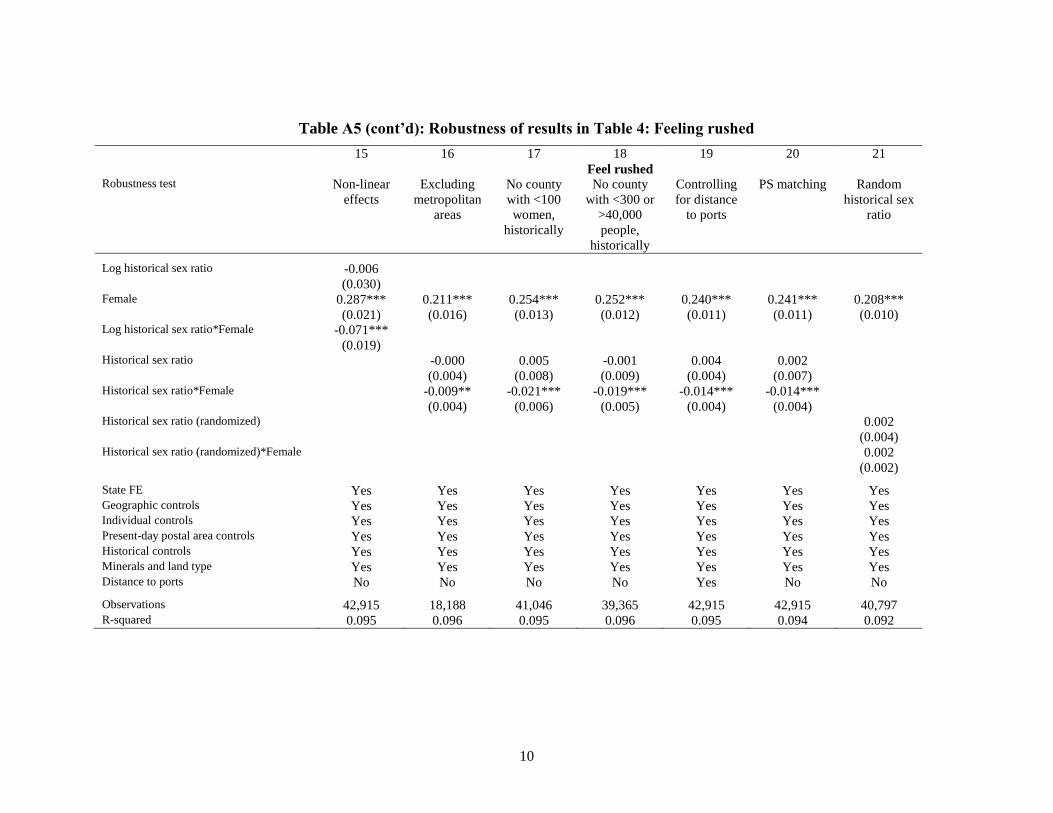
Table A5 (cont’d): Robustness of results in Table 4: Feeling rushed

15 16 17 18 19 20 21 Feel rushed Robustness test Non-linear

effects

Excluding

metropolitan

areas

No county

with <100

women,

historically

No county

with <300 or

>40,000

people,

historically

Controlling

for distance

to ports

PS matching Random

historical sex

ratio

Log historical sex ratio -0.006 (0.030) Female 0.287*** 0.211*** 0.254*** 0.252*** 0.240*** 0.241*** 0.208*** (0.021) (0.016) (0.013) (0.012) (0.011) (0.011) (0.010) Log historical sex ratio*Female -0.071*** (0.019) Historical sex ratio -0.000 0.005 -0.001 0.004 0.002 (0.004) (0.008) (0.009) (0.004) (0.007) Historical sex ratio*Female -0.009** -0.021*** -0.019*** -0.014*** -0.014*** (0.004) (0.006) (0.005) (0.004) (0.004) Historical sex ratio (randomized) 0.002

(0.004) Historical sex ratio (randomized)*Female 0.002


11

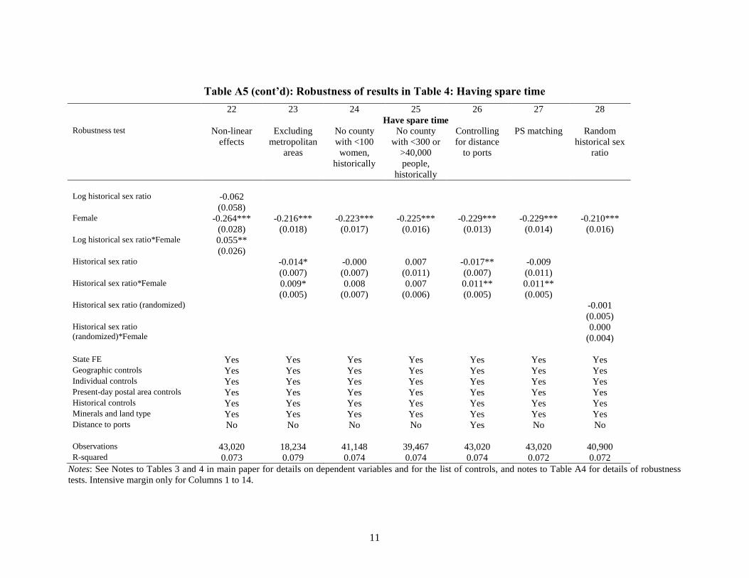
Table A5 (cont’d): Robustness of results in Table 4: Having spare time

22 23 24 25 26 27 28 Have spare time Robustness test Non-linear

effects

Excluding

metropolitan

areas

No county

with <100

women,

historically

No county

with <300 or

>40,000

people,

historically

Controlling

for distance

to ports

PS matching Random

historical sex

ratio

Log historical sex ratio -0.062 (0.058) Female -0.264*** -0.216*** -0.223*** -0.225*** -0.229*** -0.229*** -0.210*** (0.028) (0.018) (0.017) (0.016) (0.013) (0.014) (0.016) Log historical sex ratio*Female 0.055** (0.026) Historical sex ratio -0.014* -0.000 0.007 -0.017** -0.009 (0.007) (0.007) (0.011) (0.007) (0.011) Historical sex ratio*Female 0.009* 0.008 0.007 0.011** 0.011** (0.005) (0.007) (0.006) (0.005) (0.005) Historical sex ratio (randomized) -0.001


(randomized)*Female 0.000


Notes: See Notes to Tables 3 and 4 in main paper for details on dependent variables and for the list of controls, and notes to Table A4 for details of robustness

tests. Intensive margin only for Columns 1 to 14.

12

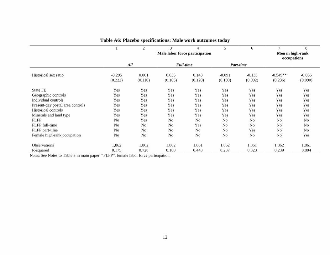
Table A6: Placebo specifications: Male work outcomes today

1 2 3 4 5 6 7 8

Male labor force participation Men in high-rank

occupations

All Full-time Part-time

Historical sex ratio -0.295 0.001 0.035 0.143 -0.091 -0.133 -0.549** -0.066

(0.222) (0.110) (0.165) (0.120) (0.100) (0.092) (0.236) (0.090)



Individual controls Yes Yes Yes Yes Yes Yes Yes Yes

Present-day postal area controls Yes Yes Yes Yes Yes Yes Yes Yes

Historical controls Yes Yes Yes Yes Yes Yes Yes Yes

Minerals and land type Yes Yes Yes Yes Yes Yes Yes Yes

FLFP No Yes No No No No No No

FLFP full-time No No No Yes No No No No

FLFP part-time No No No No No Yes No No

Female high-rank occupation No No No No No No No Yes

Observations 1,862 1,862 1,862 1,861 1,862 1,861 1,862 1,861

R-squared 0.175 0.728 0.180 0.443 0.237 0.323 0.239 0.804

Notes: See Notes to Table 3 in main paper. “FLFP”: female labor force participation.

13

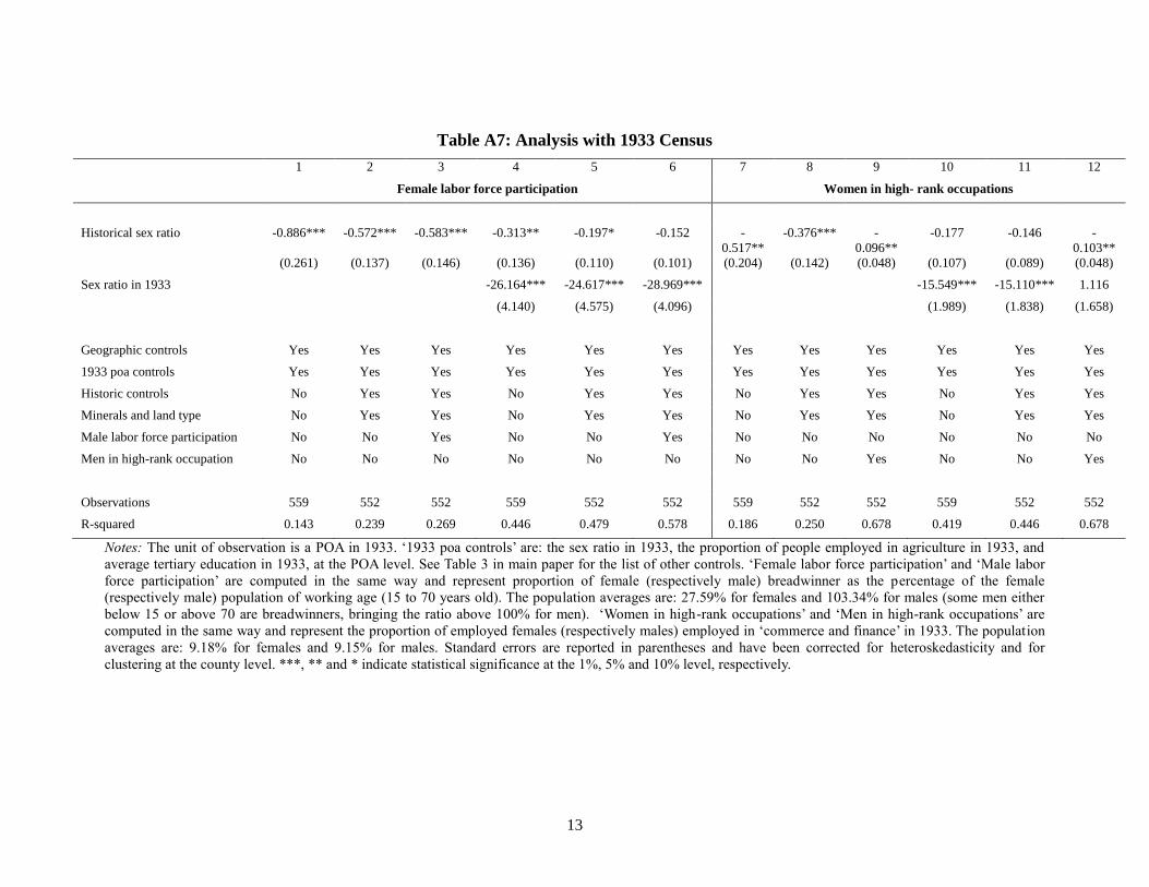
Table A7: Analysis with 1933 Census

1 2 3 4 5 6 7 8 9 10 11 12

Female labor force participation Women in high- rank occupations

Historical sex ratio -0.886*** -0.572*** -0.583*** -0.313** -0.197* -0.152 -

0.517**

-0.376*** -

0.096**

-0.177 -0.146 -

0.103**

(0.261) (0.137) (0.146) (0.136) (0.110) (0.101) (0.204) (0.142) (0.048) (0.107) (0.089) (0.048)

Sex ratio in 1933 -26.164*** -24.617*** -28.969*** -15.549*** -15.110*** 1.116

(4.140) (4.575) (4.096) (1.989) (1.838) (1.658)

Geographic controls Yes Yes Yes Yes Yes Yes Yes Yes Yes Yes Yes Yes

1933 poa controls Yes Yes Yes Yes Yes Yes Yes Yes Yes Yes Yes Yes

Historic controls No Yes Yes No Yes Yes No Yes Yes No Yes Yes

Minerals and land type No Yes Yes No Yes Yes No Yes Yes No Yes Yes

Male labor force participation No No Yes No No Yes No No No No No No

Men in high-rank occupation No No No No No No No No Yes No No Yes

Observations 559 552 552 559 552 552 559 552 552 559 552 552

R-squared 0.143 0.239 0.269 0.446 0.479 0.578 0.186 0.250 0.678 0.419 0.446 0.678

Notes: The unit of observation is a POA in 1933. ‘1933 poa controls’ are: the sex ratio in 1933, the proportion of people employed in agriculture in 1933, and

average tertiary education in 1933, at the POA level. See Table 3 in main paper for the list of other controls. ‘Female labor force participation’ and ‘Male labor

force participation’ are computed in the same way and represent proportion of female (respectively male) breadwinner as the percentage of the female

(respectively male) population of working age (15 to 70 years old). The population averages are: 27.59% for females and 103.34% for males (some men either

below 15 or above 70 are breadwinners, bringing the ratio above 100% for men). ‘Women in high-rank occupations’ and ‘Men in high-rank occupations’ are

computed in the same way and represent the proportion of employed females (respectively males) employed in ‘commerce and finance’ in 1933. The population

averages are: 9.18% for females and 9.15% for males. Standard errors are reported in parentheses and have been corrected for heteroskedasticity and for

clustering at the county level. ***, ** and * indicate statistical significance at the 1%, 5% and 10% level, respectively.

14

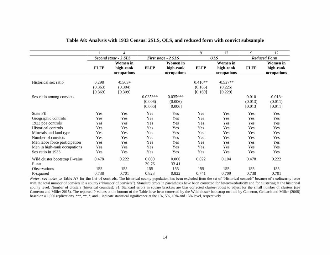
Table A8: Analysis with 1933 Census: 2SLS, OLS, and reduced form with convict subsample

1 4 9 12 9 12

Second stage - 2 SLS First stage - 2 SLS OLS Reduced Form

FLFP

Women in

high-rank

occupations

FLFP

Women in

high-rank

occupations

FLFP

Women in

high-rank

occupations

FLFP

Women in

high-rank

occupations

Historical sex ratio 0.298 -0.503+

0.410** -0.527**

(0.363) (0.304)

(0.166) (0.225)

[0.369] [0.309]

[0.169] [0.229]

Sex ratio among convicts

0.035*** 0.035***

0.010 -0.018+

(0.006) (0.006)

(0.013) (0.011)

[0.006] [0.006]

[0.013] [0.011]



1933 poa controls Yes Yes Yes Yes Yes Yes Yes Yes

Historical controls Yes Yes Yes Yes Yes Yes Yes Yes

Minerals and land type Yes Yes Yes Yes Yes Yes Yes Yes

Number of convicts Yes Yes Yes Yes Yes Yes Yes Yes

Men labor force participation Yes Yes Yes Yes Yes Yes Yes Yes

Men in high-rank occupations Yes Yes Yes Yes Yes Yes Yes Yes

Sex ratio in 1933 Yes Yes Yes Yes Yes Yes Yes Yes

Wild cluster bootstrap P-value 0.478 0.222 0.000 0.000 0.022 0.104 0.478 0.222

F-stat - - 30.76 33.41 - - - -

Observations 155 155 155 155 155 155 155 155

R-squared 0.738 0.701 0.823 0.822 0.741 0.709 0.738 0.701

Notes: see notes to Table A7 for the list of controls. The historical county population has been excluded from the set of “Historical controls” because of a colinearity issue

with the total number of convicts in a county (“Number of convicts”). Standard errors in parentheses have been corrected for heteroskedasticity and for clustering at the historical

county level. Number of clusters (historical counties): 31. Standard errors in square brackets are bias-corrected cluster-robust to adjust for the small number of clusters (see

Cameron and Miller 2015). The reported P-values at the bottom of the Table have been corrected by the Wild cluster bootstrap method by Cameron, Gelbach and Miller (2008)

based on a 1,000 replications. ***, **, *, and + indicate statistical significance at the 1%, 5%, 10% and 15% level, respectively.

15

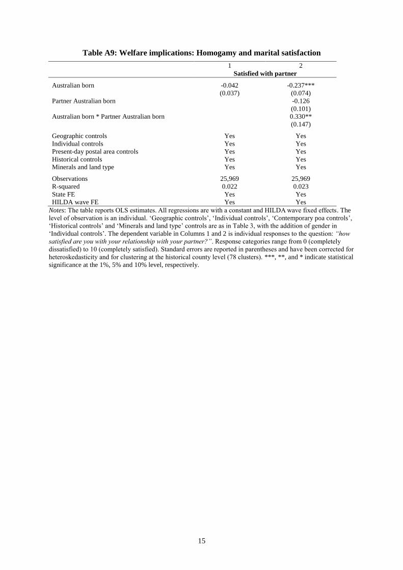
Table A9: Welfare implications: Homogamy and marital satisfaction

1 2

Satisfied with partner

Australian born -0.042 -0.237***

(0.037) (0.074)

Partner Australian born -0.126

(0.101)

Australian born * Partner Australian born 0.330**

(0.147)

Geographic controls Yes Yes

Individual controls Yes Yes

Present-day postal area controls Yes Yes

Historical controls Yes Yes

Minerals and land type Yes Yes

Observations 25,969 25,969

R-squared 0.022 0.023

State FE Yes Yes

HILDA wave FE Yes Yes

Notes: The table reports OLS estimates. All regressions are with a constant and HILDA wave fixed effects. The

level of observation is an individual. ‘Geographic controls’, ‘Individual controls’, ‘Contemporary poa controls’,

‘Historical controls’ and ‘Minerals and land type’ controls are as in Table 3, with the addition of gender in

‘Individual controls’. The dependent variable in Columns 1 and 2 is individual responses to the question: “how

satisfied are you with your relationship with your partner?”. Response categories range from 0 (completely

dissatisfied) to 10 (completely satisfied). Standard errors are reported in parentheses and have been corrected for

heteroskedasticity and for clustering at the historical county level (78 clusters). ***, **, and * indicate statistical

significance at the 1%, 5% and 10% level, respectively.

16

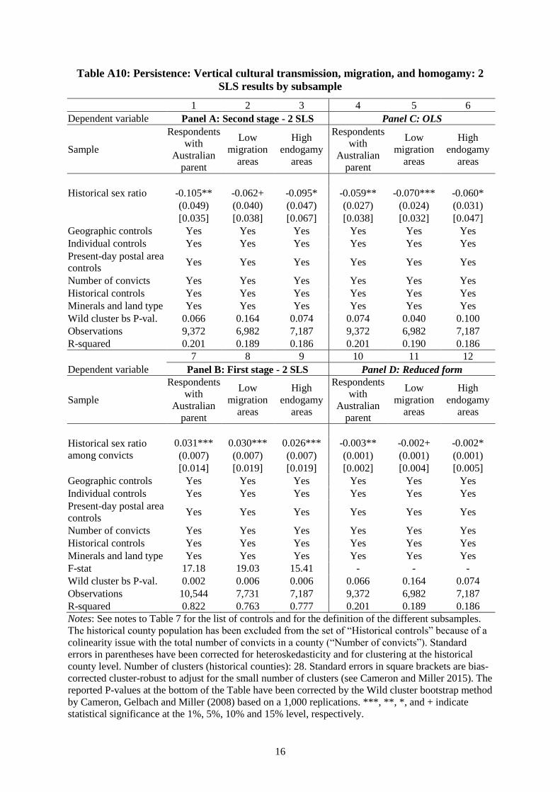
Table A10: Persistence: Vertical cultural transmission, migration, and homogamy: 2

SLS results by subsample

1 2 3 4 5 6

Dependent variable Panel A: Second stage - 2 SLS Panel C: OLS

Sample

Respondents

with

Australian

parent

Low

migration

areas

High

endogamy

areas

Respondents

with

Australian

parent

Low

migration

areas

High

endogamy

areas

Historical sex ratio -0.105** -0.062+ -0.095* -0.059** -0.070*** -0.060*

(0.049) (0.040) (0.047) (0.027) (0.024) (0.031)

[0.035] [0.038] [0.067] [0.038] [0.032] [0.047]

Geographic controls Yes Yes Yes Yes Yes Yes

Individual controls Yes Yes Yes Yes Yes Yes

Present-day postal area

controls Yes Yes Yes Yes Yes Yes

Number of convicts Yes Yes Yes Yes Yes Yes

Historical controls Yes Yes Yes Yes Yes Yes

Minerals and land type Yes Yes Yes Yes Yes Yes

Wild cluster bs P-val. 0.066 0.164 0.074 0.074 0.040 0.100

Observations 9,372 6,982 7,187 9,372 6,982 7,187

R-squared 0.201 0.189 0.186 0.201 0.190 0.186

7 8 9 10 11 12

Dependent variable Panel B: First stage - 2 SLS Panel D: Reduced form

Sample

Respondents

with

Australian

parent

Low

migration

areas

High

endogamy

areas

Respondents

with

Australian

parent

Low

migration

areas

High

endogamy

areas

Historical sex ratio

among convicts

0.031*** 0.030*** 0.026*** -0.003** -0.002+ -0.002*

(0.007) (0.007) (0.007) (0.001) (0.001) (0.001)

[0.014] [0.019] [0.019] [0.002] [0.004] [0.005]

Geographic controls Yes Yes Yes Yes Yes Yes

Individual controls Yes Yes Yes Yes Yes Yes

Present-day postal area

controls Yes Yes Yes Yes Yes Yes

Number of convicts Yes Yes Yes Yes Yes Yes

Historical controls Yes Yes Yes Yes Yes Yes

Minerals and land type Yes Yes Yes Yes Yes Yes

F-stat 17.18 19.03 15.41 - - -

Wild cluster bs P-val. 0.002 0.006 0.006 0.066 0.164 0.074

Observations 10,544 7,731 7,187 9,372 6,982 7,187

R-squared 0.822 0.763 0.777 0.201 0.189 0.186

Notes: See notes to Table 7 for the list of controls and for the definition of the different subsamples.

The historical county population has been excluded from the set of “Historical controls” because of a

colinearity issue with the total number of convicts in a county (“Number of convicts”). Standard

errors in parentheses have been corrected for heteroskedasticity and for clustering at the historical

county level. Number of clusters (historical counties): 28. Standard errors in square brackets are bias-

corrected cluster-robust to adjust for the small number of clusters (see Cameron and Miller 2015). The

reported P-values at the bottom of the Table have been corrected by the Wild cluster bootstrap method

by Cameron, Gelbach and Miller (2008) based on a 1,000 replications. ***, **, *, and + indicate

statistical significance at the 1%, 5%, 10% and 15% level, respectively.

17

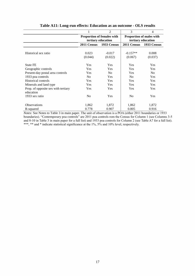
Table A11: Long-run effects: Education as an outcome - OLS results

1 2 3 4

Proportion of females with

tertiary education

Proportion of males with

tertiary education

2011 Census 1933 Census 2011 Census 1933 Census

Historical sex ratio 0.023 -0.017 -0.157** 0.008

(0.044) (0.022) (0.067) (0.037)

State FE Yes Yes Yes Yes

Geographic controls Yes Yes Yes Yes

Present-day postal area controls Yes No Yes No

1933 poa controls No Yes No Yes

Historical controls Yes Yes Yes Yes

Minerals and land type Yes Yes Yes Yes

Prop. of opposite sex with tertiary

education

Yes Yes Yes Yes

1933 sex ratio No Yes No Yes

Observations 1,862 1,872 1,862 1,872

R-squared 0.778 0.907 0.805 0.916

Notes: See Notes to Table 3 in main paper. The unit of observation is a POA (either 2011 boundaries or 1933

boundaries). “Contemporary poa controls” are 2011 poa controls rom the Census for Column 1 (see Columns 3-5

and 8-10 in Table 3 in main paper for a full list) and 1933 poa controls for Column 2 (see Table A7 for a full list).

***, ** and * indicate statistical significance at the 1%, 5% and 10% level, respectively.

18

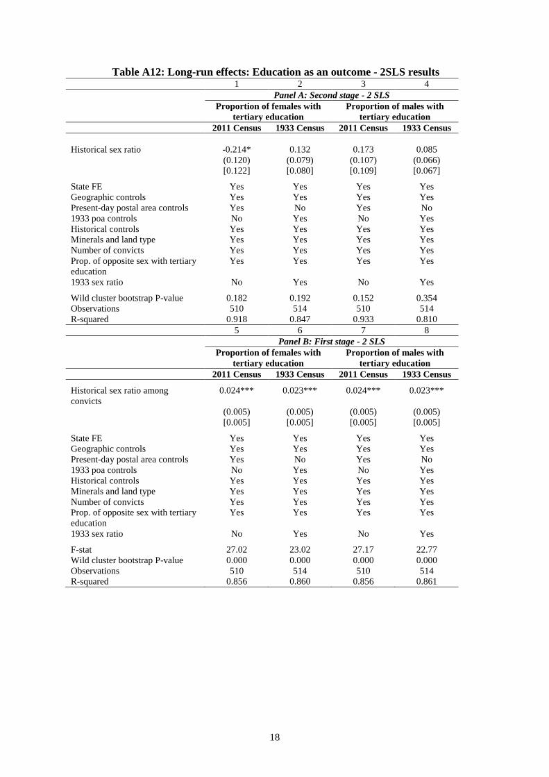
Table A12: Long-run effects: Education as an outcome - 2SLS results 1 2 3 4

Panel A: Second stage - 2 SLS


tertiary education


tertiary education


Historical sex ratio -0.214* 0.132 0.173 0.085

(0.120) (0.079) (0.107) (0.066)

[0.122] [0.080] [0.109] [0.067]







Number of convicts Yes Yes Yes Yes


education

Yes Yes Yes Yes


Wild cluster bootstrap P-value 0.182 0.192 0.152 0.354

Observations 510 514 510 514

R-squared 0.918 0.847 0.933 0.810

5 6 7 8

Panel B: First stage - 2 SLS


tertiary education


tertiary education


Historical sex ratio among

convicts

0.024*** 0.023*** 0.024*** 0.023***

(0.005) (0.005) (0.005) (0.005)

[0.005] [0.005] [0.005] [0.005]









education

Yes Yes Yes Yes


F-stat 27.02 23.02 27.17 22.77



R-squared 0.856 0.860 0.856 0.861

19

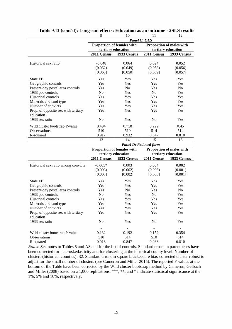
Table A12 (cont’d): Long-run effects: Education as an outcome - 2SLS results 9 10 11 12

Panel C: OLS


tertiary education


tertiary education


Historical sex ratio -0.048 0.064 0.024 0.052

(0.062) (0.049) (0.058) (0.056)

[0.063] [0.050] [0.059] [0.057]









education

Yes Yes Yes Yes




R-squared 0.917 0.932 0.847 0.810

13 14 15 16

Panel D: Reduced form


tertiary education


tertiary education


Historical sex ratio among convicts -0.005* 0.003 0.004 0.002

(0.003) (0.002) (0.003) (0.001)

[0.003] [0.002] [0.003] [0.001]









education

Yes Yes Yes Yes


- - - -



R-squared 0.918 0.847 0.933 0.810

Notes: See notes to Tables 5 and A8 and for the list of controls. Standard errors in parentheses have

been corrected for heteroskedasticity and for clustering at the historical county level. Number of

clusters (historical counties): 32. Standard errors in square brackets are bias-corrected cluster-robust to

adjust for the small number of clusters (see Cameron and Miller 2015). The reported P-values at the

bottom of the Table have been corrected by the Wild cluster bootstrap method by Cameron, Gelbach

and Miller (2008) based on a 1,000 replications. ***, **, and * indicate statistical significance at the

1%, 5% and 10%, respectively.

20

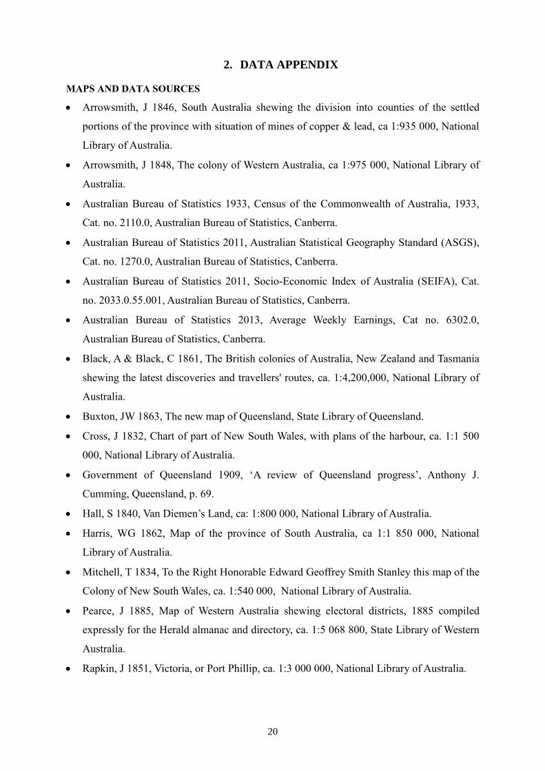
2. DATA APPENDIX

MAPS AND DATA SOURCES

Arrowsmith, J 1846, South Australia shewing the division into counties of the settled

portions of the province with situation of mines of copper & lead, ca 1:935 000, National

Library of Australia.

Arrowsmith, J 1848, The colony of Western Australia, ca 1:975 000, National Library of

Australia.

Australian Bureau of Statistics 1933, Census of the Commonwealth of Australia, 1933,

Cat. no. 2110.0, Australian Bureau of Statistics, Canberra.

Australian Bureau of Statistics 2011, Australian Statistical Geography Standard (ASGS),

Cat. no. 1270.0, Australian Bureau of Statistics, Canberra.

Australian Bureau of Statistics 2011, Socio-Economic Index of Australia (SEIFA), Cat.

no. 2033.0.55.001, Australian Bureau of Statistics, Canberra.

Australian Bureau of Statistics 2013, Average Weekly Earnings, Cat no. 6302.0,

Australian Bureau of Statistics, Canberra.

Black, A & Black, C 1861, The British colonies of Australia, New Zealand and Tasmania

shewing the latest discoveries and travellers' routes, ca. 1:4,200,000, National Library of

Australia.

Buxton, JW 1863, The new map of Queensland, State Library of Queensland.

Cross, J 1832, Chart of part of New South Wales, with plans of the harbour, ca. 1:1 500

000, National Library of Australia.

Government of Queensland 1909, ‘A review of Queensland progress’, Anthony J.

Cumming, Queensland, p. 69.

Hall, S 1840, Van Diemen’s Land, ca: 1:800 000, National Library of Australia.

Harris, WG 1862, Map of the province of South Australia, ca 1:1 850 000, National

Library of Australia.

Mitchell, T 1834, To the Right Honorable Edward Geoffrey Smith Stanley this map of the

Colony of New South Wales, ca. 1:540 000, National Library of Australia.

Pearce, J 1885, Map of Western Australia shewing electoral districts, 1885 compiled

expressly for the Herald almanac and directory, ca. 1:5 068 800, State Library of Western

Australia.

Rapkin, J 1851, Victoria, or Port Phillip, ca. 1:3 000 000, National Library of Australia.

21

Robertson, A 1858, Victoria, census districts and distribution of the population, March

29th 1857, ca. 1:510 000, National Library of Australia.

Waterlow & Sons 1859, Map of South Australia including the recent discoveries, ca 1

inch to 20 miles, State Library of South Australia.

Note: 12 counties from the Colonial Censuses had to be dropped because of incomplete maps.

22

1 Historical Variables

1.1 First historical cross section for use in present-day regressions

Data from the first historical cross section is taken from the Historical Census and Colonial Data

Archive (HCCDA) (See Table A13). The HCCDA is an online archive containing the reports of each

colonial Census administered in Australia, prior to Federation in 1901.1 For all historical variables, the

unit of observation is the county or police district (as applicable). The first Censuses administered on

this micro level are used to calculate the gender ratio for all colonies, except NSW where the second

Census is used. NSW’s first Census on the county level was in 1833. However, adequate information

on county boundaries is not available for NSW until 1834 when Surveyor General Major Thomas

Mitchell was commissioned to map NSW into 19 formal counties. As a result, for NSW we use the

second Census, which occurred in 1834. Similarly, occupation data on men and women is taken from

the Census in which it is first available.

Only the Census reports are available consistently across the relevant period, as some of the

individual records were destroyed in a fire in 1882.

Table A13: First historical cross section – the Censuses

Variable Description Colony Year of Census

Convict gender ratio Number of convict

men to the number of

convict women

New South Wales 1834

Tasmania 1842

Historical gender

ratio

Number of men to

the number of

women


Queensland 1861

South Australia 1844, 1861

Tasmania 1842

Victoria 1854

Western Australia 1848

Proportion of

married men

Number of married

men to the number of

men in the county


Queensland 1861


Tasmania 1842

Victoria 1854


Proportion of

married women

Number of married

women to the

number of women in

the county


Queensland 1861


Tasmania 1842

Victoria 1854


Occupation data Number of men and

women working in a

range of occupations


Queensland 1861

South Australia 1861

Tasmania 1881

1 For the 1881 Tasmanian census, the HCCDA was supplemented by the actual Census report

due to errors.

23

Victoria 1854

Western Australia 1881 Notes: These dates vary because states were independent colonies until 1901.

1.2 Historical panel data (1836 - 1881)

Similar to the above, data for the historical panel is also taken from the HCCDA (See Table A14).

Once again, each variable is observed at the county or police district level.

Table A14: Description of historical panel variables

Variable Description

Sex ratio Number of men to the number of women

Female Labor Force

Participation

Proportion of females employed, as a proportion of married females

Male Labor Force

Participation

Proportion of males employed, as a proportion of married males

Women in high-ranking

occupations

Proportion of women employed in ‘commerce and finance’, as a

percentage of the employed females

Male high-ranking

occupations

Proportion of men employed in ‘commerce and finance’, as a

percentage of the employed men

The historical panel is sourced from 19th Century Censuses. Table A1 provides a detailed breakdown

of the years in which the variables were taken and the number of counties observed at each point in

time.

For the historical panel year and number of counties, see Table A1.

2 Present-day variables

2.1 Household, Income and Labor Dynamics in Australia (HILDA) Survey

HILDA is a nationally representative survey available since 2001. For our paper, variables taken from

the HILDA survey (See Table A16) are observed in 2001, 2005, 2008 and 2011, as these are the years

respondents have been asked their attitudes towards gender roles. HILDA provides a vast array of

information on households and individuals who are representative of the Australian

population. Adult members of households are interviewed annually and are asked to complete

a questionnaire. We are interested in these ‘responding persons’ as information on attitudinal

variables are provided for them.

For all HILDA variables, the unit of observation is an individual living in a postal area at each point in

time – matched to a historic county (matching process described in Section 3 bellow).

24

Table A15: Description of HILDA variables


Progressive Attitude Gender Roles An individual’s response to the statement: “it is

better for everyone involved if the man earns the

money and the woman takes care of the home and

children.” Response categories range from 1

(strongly disagree) to 7 (strongly agree), which

we recoded so that a higher value indicates more

progressive attitudes.

Time spent with children

Tim use date that includes: playing with children,

helping them with personal care, teaching,

coaching, or actively supervising them and

getting them to day care, school, or other

activities

Time spent in housework and household errands

Time use data that includes: preparing meals,

washing dishes, cleaning house, washing clothes,

ironing, sewing, shopping, banking, paying bills,

and keeping financial records.

Feel rushed

An individual’s response to the question: “How

often to you feel rushed or pressed for time?”

Response categories range from 1 (never) to 5

(almost always).

Have spare time

An individual’ response to the question: “How

often to you have spare time that you don’t know

what to do with?” Response categories range

from 1 (never) to 5 (almost always).

Log hours worked

Log of answers to the question: “How many

hours per week do you usually worked in all

jobs?”. We have added 1 to all answers to avoid

non defined numbers and obtain values of 0 for

those who report 0 hours worked.

Married or de facto Dummy variable equal to one if an individual is

married or in a de facto relationship

Age An individual’s age

Beyond year 12 education

Dummy variable equal to one if the individual

has education beyond year 12 (that is, high

school)

Australia born Dummy variable equal to one if the individual is

born in Australia

Australian parent Dummy variable equal to one if the individual

has an Australian father or an Australian mother

Female Dummy variable equal to one if the individual is

a female.

2.2 2011 Census

We also take data from the most recent Australian Census, taken in 2011.2011 Census controls are

observed at the postal area. The only construction required is matching them to the postal area of the

individual observed in HILDA.

25

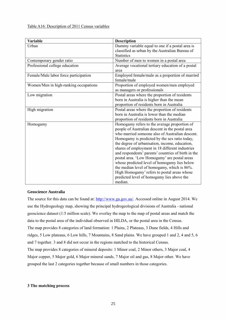
Table A16: Description of 2011 Census variables


Urban

Dummy variable equal to one if a postal area is

classified as urban by the Australian Bureau of

Statistics

Contemporary gender ratio Number of men to women in a postal area

Professional college education Average vocational tertiary education of a postal

area

Female/Male labor force participation Employed female/male as a proportion of married

female/male

Women/Men in high-ranking occupations Proportion of employed women/men employed

as managers or professionals

Low migration Postal areas where the proportion of residents

born in Australia is higher than the mean

proportion of residents born in Australia

High migration Postal areas where the proportion of residents

born in Australia is lower than the median

proportion of residents born in Australia

Homogamy Homogamy refers to the average proportion of

people of Australian descent in the postal area

who married someone also of Australian descent.

Homogamy is predicted by the sex ratio today,

the degree of urbanisation, income, education,

shares of employment in 18 different industries

and respondents’ parents’ countries of birth in the

postal area. ‘Low Homogamy’ are postal areas

whose predicted level of homogamy lies below

the median level of homogamy, which is 86%.

High Homogamy’ refers to postal areas whose

predicted level of homogamy lies above the

median.

Geoscience Australia

The source for this data can be found at: http://www.ga.gov.au/. Accessed online in August 2014. We

use the Hydrogeology map, showing the principal hydrogeological divisions of Australia - national

geoscience dataset (1:5 million scale). We overlay the map to the map of postal areas and match the

data to the postal area of the individual observed in HILDA, or the postal area in the Census.

The map provides 8 categories of land formation: 1 Plains, 2 Plateaus, 3 Dune fields, 4 Hills and

ridges, 5 Low plateaus, 6 Low hills, 7 Mountains, 8 Sand plains. We have grouped 1 and 2, 4 and 5, 6

and 7 together. 3 and 8 did not occur in the regions matched to the historical Census.

The map provides 8 categories of mineral deposits: 1 Minor coal, 2 Minor others, 3 Major coal, 4

Major copper, 5 Major gold, 6 Major mineral sands, 7 Major oil and gas, 8 Major other. We have

grouped the last 2 categories together because of small numbers in those categories.

3 The matching process

http://www.ga.gov.au/

26

To study the long-run implications of male-biased sex ratios we matched contemporary data sets

(HILDA, 2011 Census and Geoscience Australia – described above) to our historical data set.

Contemporary data sets are observed at the postal area level, while our historical data set is observed

at the county or police district levels. Postal areas are not equivalent to historical counties. To account

for this, and match the historical counties and police districts to each postal area, we use the ABS’

Australian Statistical Geography Standard (ASGS) (2011) shape file dividing Australia into polygons.

Each polygon represents one of the 2,515 Australian postal areas, as distributed in 2011.

We manually match each postal area to a historical county or police district for all our historical data

sets (first historical cross-section and panel). To do this, we combined the Australia postal area shape

file with a number of shape files containing polygons representing the historic census boundaries for

each of the colonies.2 Prior to this study, digitized shapefiles on Australian historical Census

boundaries did not exist. We collected and digitized hard copies of maps from the National Library of

Australia and from State Libraries in order to construct these boundaries and match historical counties

to present-day boundaries. When a postal area was found in multiple counties, we assigned it to the

county in which it was mostly located.

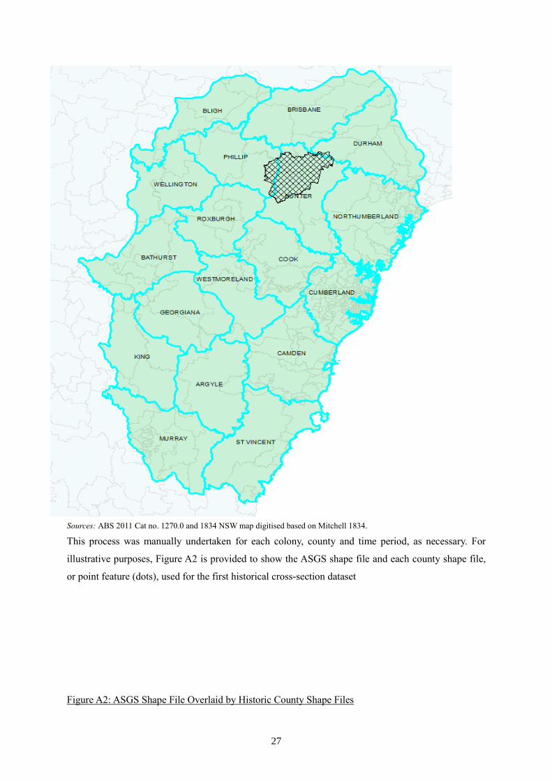
The matching process undertaken is illustrated through an example of the colony of NSW. Figure A1

provides a shape file of NSW counties in 1834, which was used in the first historic cross-section. The

highlighted polygons each represent a county. Underlying this historic map are polygons comprising

of NSW postal areas. Each postal area polygon was matched to its associated county polygon. As is

illustrated, some postal area polygons are found in multiple counties. For instance, postal area 2328,

shown in black, is located in the counties of Hunter, Phillip and Durham. To counter this, the postal

area was assigned to the county in which its polygon was mostly located. For 2328, this was Hunter.

Figure A1: ASGS Shape File Overlaid by 1834 NSW Shape File

2 Some counties had to initially be dropped as no reliable maps at a time close to the census were found.

27

Sources: ABS 2011 Cat no. 1270.0 and 1834 NSW map digitised based on Mitchell 1834.

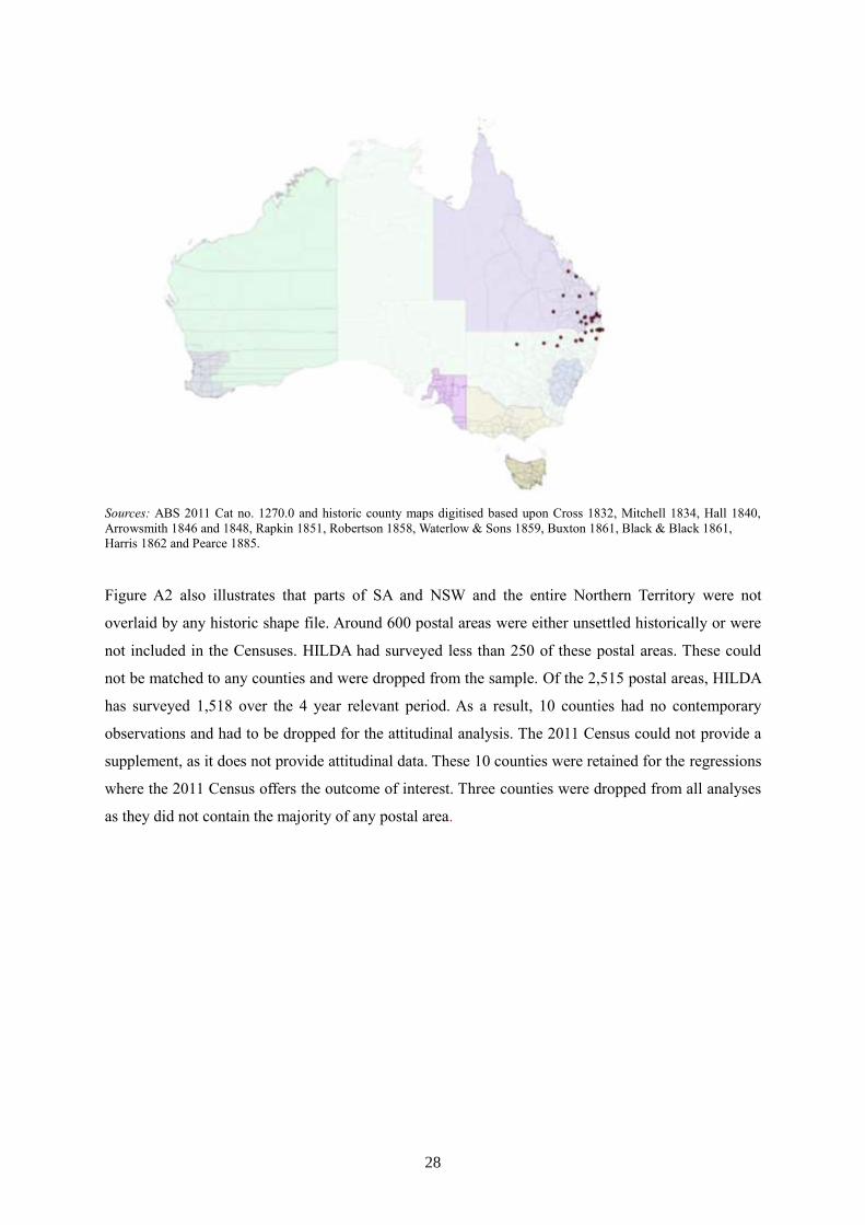
This process was manually undertaken for each colony, county and time period, as necessary. For

illustrative purposes, Figure A2 is provided to show the ASGS shape file and each county shape file,

or point feature (dots), used for the first historical cross-section dataset

Figure A2: ASGS Shape File Overlaid by Historic County Shape Files

28

Sources: ABS 2011 Cat no. 1270.0 and historic county maps digitised based upon Cross 1832, Mitchell 1834, Hall 1840,

Arrowsmith 1846 and 1848, Rapkin 1851, Robertson 1858, Waterlow & Sons 1859, Buxton 1861, Black & Black 1861,

Harris 1862 and Pearce 1885.

Figure A2 also illustrates that parts of SA and NSW and the entire Northern Territory were not

overlaid by any historic shape file. Around 600 postal areas were either unsettled historically or were

not included in the Censuses. HILDA had surveyed less than 250 of these postal areas. These could

not be matched to any counties and were dropped from the sample. Of the 2,515 postal areas, HILDA

has surveyed 1,518 over the 4 year relevant period. As a result, 10 counties had no contemporary

observations and had to be dropped for the attitudinal analysis. The 2011 Census could not provide a

supplement, as it does not provide attitudinal data. These 10 counties were retained for the regressions

where the 2011 Census offers the outcome of interest. Three counties were dropped from all analyses

as they did not contain the majority of any postal area.

Documents

For Online Publication Only APPENDIX: It’s Raining Men ...p3.storage.canalblog.com/32/34/1099015/113460587.pdf · 1 For Online Publication Only APPENDIX: It’s Raining Men! Hallelujah?