DOCUMENT RFSUM?

ED 045 349 SF 009 211

APTHORT1-7LEINSTITUTIONSPONS AGENCYnTIP PATENoTE

Frog DRICEDES7RIPTORS

rearlman, NormanHeat and Motion.Commission on Coll. physics, College Park, 10.National Science Foundation, Washington, D.C.A 6

l'a.; Monoaraph vritten for the Conference on theNew Instructional Materials in Physics (Universityof Washington, Seattle, 19(5)

FOPS Price MF-$0.0 PC-5?-95*Colleae Science, *Instructional Materials,*Physics, *Quantum Mechanics, *Thermodynamics

APqTPACTUnlike many elementary presentations on heat, this

monograph is not restricted to exPlaining thermal behavior in onlymacroscopic terms, but also developer the relationships betweenthermal properties and atomic vehavior. "It relies at the start onintuition about heat at the macroscopic level. ramiliarity with thenarticle model of mechanics, which is assumed from an earlier course,is used to develop an understanding of temperature and heat inmacroscopic terms. Tt then relates these ideas to behavior of theinternal degrees of freedom in macroscopic oblects, and shows thatthese degrees of freedom behave differently from what would heaxpoctel if they simply mimicked large -scale notion. In this way,contact is made with discussion of auantum mechanics elsewhere."Topics are: Model - Building in Physics; The Particle Model for Motion;The Direction of the Flow of Time; Temperature and ThermalT:auilibrium; to Thermal Equilihrilm States Fxist?; and Internal')eirees of FrcOcm. (Author/Ps)

1

ILw

1

1

U S DEPARTMENT OF PIAIIK, EDUCATION & WELFARE

OFFiCE OF EDUCATION

THIS DOCUMENT PAS IMF REPRODUCED (VICHY AS RECEIVED FROM DIE

PERSON OR ORGANIZATION ORIGINATING It POINTS Of VIEW OR OPINIONS

STATED DO NOT NECESSARILY REPRESENT OFFICIAL OFFICE Of EDUCATION

POSITION Of POLICY

"PERMISSION TO PRODUCE THISCOPYRIGHTED MATERIAL HAS DEIN GRANTED

sy Ronald GE.balle

10 ERIC AND ORGANIZATIONS OPERATING

UNDER AGREEMENTS WITH THE U.S. OFFICE OF

EDUCATION. FURTHER REPRODUCTION OUTSIDE

THE ERIC SYSTEM !SHIRES PERMISSIOP OF

THE COPYRIGHT OWNER."

GENERAL PREFACE

This monograph was written for the Conference on the New Instructional

Materials in Physics, held at the University of Washington in the sum-

mer of 1965. The general purpose of the conference was to create effec-

tive ways of presenting physics to college students who are not pre-

paring to become professional physicists. Such an audience might include

prospective secondary school physics teachers, prospective practitioners

of other sciences, and those who wish to learn physics as one component

of a liberal education.

At the Conference some 40 physicists and 12 filmmakers and design-

ers worked for periods ranging from four to nine weeks. The central

task, certainly the one in which most physicists participated, was the

writing of monographs.

Although there was no consensus on a single approach, many writers

felt that their presentations ought to put more than the customary

emphasis on physical insight and synthesis. Moreover, the treatment was

to be "multi-level" --- that is, etch monograph would consist of sev-

eral sections arranged in increasing order of sophistication. Such

papers, it was hoped, could be readily introduced into existing courses

or provide the basis for new kinds of courses.

Monographs were written in four content areas: Forces and Fields,

Quantum Mechanics, Thermal and Statistical Physics, and the Structure

and Properties of Matter. Topic selections and general outlines were

only loosely coordinated within each area in order to leave authors

free to invent new approaches. In point of fact, however, a number of

monographs do relate to others in complementary ways, a result of their

authors' close, informal interaction.

Because of stringent time limitations, few of the monographs have

been completed, and none has been Ixtensively rewritten. Indeed, most

writers feel that they are barely more than clean first drafts. Yet,

because of the highly experimental nature of the undertaking, it is

essential that these manuscripts be made available for careful review

by other physicists and for trial use with students. Much effort,

therefore, has gone into publishing them in a readable format intended

to facilitate serious consideration.

So many people have contributed to the project that complete

acknowledgement is not possible. The National Science Foundation sup-

ported the Conference. The staff of the Commission on College Physics,

led by E. Leonard Jossem, and that of the University of Washington

physics department, led by Ronald Geballe and Ernest M. Henley, car-

ried the heavy burden of organization. Walter C. Michels, Lyman G.

Parratt, and George M. Volkoff read and criticized manuscripts at a

critical stage in the writing. Judith Bregman, Edward Gerjuoy, Ernest

M. Henley, and Lawrence Wilets read manuscripts editorially. Martha

Ellis and Margery Lang did the technical editing; Ann Widditsch

supervised the initial typing and assembled the final drafts. James

Grunbaum designed the format and, assisted in Seattle by Roselyn Pape,

directed the art preparation. Richard A. Mould has helped in all phases

of readying manuscripts for the printer. :finally, and crucially, Jay F.

Wilson, of the D. Van Nostrand Company, served as Managing Editor. For

the hard work and steadfast support of all these persons and many

others, I am deeply grateful.

Edward D. LambeChairman, Panel on theNew Instructioncl MaterialsCommission on College Physics

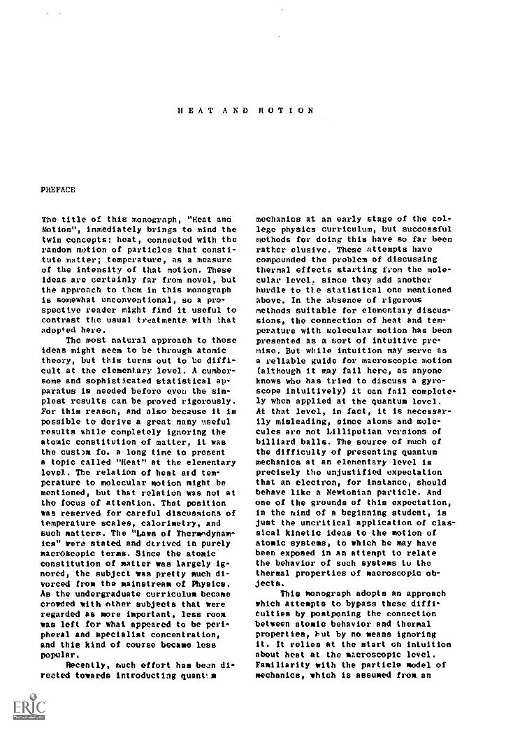
HEAT AND MOTION

PREFACE

The title of this monograph, "Heat andMotion", immediately brings to mind thetwin concepts: heat, connected with therandom motion of particles that consti-tute matter; temperature, as a measureof the intensity of that motion. Theseideas are certainly far from novel, butthe approach to them in this monographis somewhat unconventional, so a pro-spective reader might find it useful tocontrast the usual treatments with thatadopted here.

The most natural approach to theseideas might seem to be through atomictheory, but this turns out to be diffi-cult at the elementary level. A cumber-some and sophisticated statistical ap-paratus is needed before even the sim-plest results can be proved rigorously.For this reason, and also because it ispossible to derive a great many usefulresults while completely ignoring theatomic constitution of matter, it wasthe cust3m fo. a long time to presenta topic called "Heat" at the elementarylevel. The relation of heat and tem-perature to molecular motion might bementioned, but that relation was not atthe focus of attention. That positionwas reserved for careful discussions oftemperature scales, calorimetry, andsuch matters. The "Laws of Thermodynam-ics" were stated and dtrived in purelymacroscopic terms. Since the atomicconstitution of matter was largely ig-nored, the subject was pretty much di-vorced from the mainstream of Physics.As the undergraduate curriculum becamecrowded with other subjects that wereregarded as more important, less roomwas left for what appeared to be peri-pheral and specialist concentration,and this kind of course became lesspopular.

Recently, much effort has bean di-rected towards introducting quant!A

mechanics at an early stage of the col-lege physics curriculum, but successfulmethods for doing this have so far beenrather elusive. These attempts havecompounded the problem of discussingthermal effects starting from the mole-cular level. since they add anotherhurdle to tie statistical one mentionedabove. In the absence of rigorousmethods suitable for elementary discus-sions, the connection of heat and tem-perature with molecular motion has beenpresented as a sort of intuitive pre-mise. But while intuition may serve asa reliable guide for macroscopic motion(although it may fail here, as anyoneknows who has tried to discuss a gyro-scope intuitively) it can fail complete-ly when applied at the quantum level.At that level, in fact, it is necessar-ily misleading, since atoms and mole-cules are not Lilliputian versions ofbilliard balls. The source of much ofthe difficulty of presenting quantummechanics at an elementary level isprecisely the unjustified expectationthat an electron, for instance, shouldbehave like a Newtonian particle. Andone of the grounds of this expectation,in the mind of a beginning student, isjust the uncritical application of clas-sical kinetic ideas to the motion ofatomic systems, to which he may havebeen exposed in an attempt to relatethe behavior of such systems to thethermal properties of macroscopic ob-jects.

This monograph adopts an approachwhich attempts to bypass these diffi-culties by postponing the connectionbetween atomic behavior and thermalproperties, but by no means ignoringit. It relies at the start on intuitionabout heat at the macroscopic level.Familiarity with the particle model ofmechanics, which is assumed from an

earlier course, is used to develop anunderstanding of temperature and hestin macroscopic terms. It then relatesthese ideas to behavior of the internaldegrees of freedom in macroscopic ob-jects, and shows that these degrees offreedom behave differently from whatwould be expected if they simply mim-icked large-scale motion. In this way,contact is made with discussion ofquantum mechanics elsewhere.

One of the major threads in thediscussion here is the contrast betweenthe behavior of thermal systems, whichmove spontaneously towards the uniform-ity of equilibrium, and the ideal re-versible behavior of classical particles.Besides providing a natural introduc-tion to the investigation of the intern-al degrees of freedom, this theme servesas a link between classical and quantumbehavior.

The argument is carried as far aspossible, without becoming involved indetailed quantitative calculations. Itassumes familiarity with simple differ-entiation and integration, in additionto a first course in elementary physics.Some of the mathematical details, andsome topics which require treatment ingreater detail that those in the textproper, are presented in Appendices.

The development sketched above canobviously be carried far beyond thepoint reached in this monograph. As itstands, it can be used as an introduc-tion to a course which surveys thermo-

dynamics and statistical mechanics. Butit might also find a place in a lessconventional course, one which soughtto trace the development of quantummechanics from classical ideas. It pro-vides an example of the motivation ofthat development which is not as com-monly stressed as others which are lessdirectly related to "classical" macro-scopic experiments.

A recent discussion of the differ-ent ways in which various theories inphysics have developed included thefollowing comment:

"Two poles...are found: oneattracts the minds thatthirst for an explanation ofthe world; the other aggregate(attracts) those who lookfor order in the world, nomatter what that order maymean. Thermodynamics wasbuilt by the second tribe,atomic theory by the first."

Granting this to be an accurate de-scription of the historical originsof these two disciplines, it is never-theless possible to believe that theyno longer need be regarded as polar op-posites, and this monograph is writtenwith that conviction.

The apparatus in Fig. 6.1 was con-structed by Professor H. Daw, whokindly proviled the photograph, andalso Figs. 6.2 and 6.3.

CONTENTS

1 MODEL-BUILDING IN PHYSICS

2 THE PARTICLE MODEL FOR MOTION 3

2.1 An example of model-building2,2 Mechanical states in the particle ride'_

3 THE DIRECTION OF THE FLOW OF TIME 8

3.1 Time reversal in the particle model3.2 The irreversibility of natural motions

4 TEMPERATURE AND THERMAL EQUILIBRIUM 13

4.1 Thermal equilibrium and the definitionof "teoperaturen

4.2 Temperature scales

5 DO THERMAL EQUILIBRIUM STATES EXIST? 24

5.1 Fluctuations in thermal properties5.2 Mechanical fluctuations5.3 Boltzmann's constant

6 INTERNAL DEGREES OF FREEDOM 39

6.1 Regularity in random events6.2 Internal energy6.3 Heat and heat capacit/

Appendix 1 TERMINAL SPEED 54

Appendix 2 FRICTIONAL FORCES AND MECHANICAL ENERGY 59

Appendix 3 ZERO TEMPERATURE ON THE OAS-THERMOMETERSCALE 61

Appendix 4 INTERCOMPARISON OF TEMPERATURE SCALES 6?

Appendix 5 INTERNAL DEGREES OF FREEDOM AND THE ATOMICMODEL 69

1 MODEL-BUILDING IN PHYSICS

In studying heat and temperature weare dealing with ideas which are sodeeply imbedded in common experiencethat we should expect them to pervadeall of physics. But strangely, thestudent of mechanics hears hardly anymention of heat or temperature, yetmechanics is supposed to be the basicsubject in physics. He likewise findsheat and temperature missing in hisstudy of electricity, of magnetism, ofoptics. Let us try to see how this pe-culiar situation comes about. This ef-fort will illuminate the interconnec-tions among all of these subjects. Itwill also confirm the original expec-tation that heat and temperature aredeeply involved in all natural phenom-ena, and help us to understand howthis involvement is best expressed inprecise physical terms.

Our puzzle is related to a ques-tion once posed to Albert Einstein. Hewas reminded that the Chinese had de-veloped the compass, gunpowder, andprinting by the fifteenth century andso were at that time far more advancedin science than Europe. Yet the Chineseproceeded very little further, whilewestern civilization since the fif-teenth century has been characterizedby an enormous increase in the abilityto understand and control nature. Why,Einstein was asked, did the Chinesefail to advance while the West, onceso far behind, outstripped then?

Many answers to this questionhave been suggested, based on supposeddifferences in the basic outlook unlife in the East as compared to theWest. But Einstein's answer was sim-pler: it was that the failure of theChinese was not surprising - the won-der was that progress was made any-where, considering the complexity ofnatural phenomena.

In Europe, it happened that tech-niques of investigation were developedwhich facilitated this progress. Thisdevelopment, as we look back on it,

1

was not due to a conscious analysis ofwhat we now call the "scientific meth-od." Some direct efforts of this kindwere made, but they seem now to havebeen mostly sterile. Rather, progresswas the result of trial and error; the"breakthrough," as newspapers wouldcall it nowadays, was largely a :Patterof chance.

The techniques for investigatingnature which turn out to be successfulare based on a curious fact: It isprofitable to approach the understand-ing of natural phenomena in what ap-pears to be an indirect manner. Insteadof trying to describe all aspects of acomplicated phenomenon together, asimplified version is invented by iso-lating those factors which are of spe-cial importance to the particular prob-lem under consideration. In this proc-ess of selection it is often convenientto consider the behavior of an inventedabstract model rather than that of thereal physical object involved in thephenomenon. The model can then be givensuch properties, and can be requiredto obey such physical laws, as resultin behavior which reproduces the im-portant aspects of the actual phenom-enon. The criterion of "importance,"of course, is decided in terms of eachparticular problem that is being in-vestigated. The model and its proper-ties, together with the physical laws,make up a theory of the phenn'ienonwhich can be tested by comparing itspredictions with the actual observedbehavior.'

iSometises the whole collection of concepts -abstract model (of the physical object), itsproperties and the physical laws are referred tocollectively as a "model of the phenomenon."this can be confusing, and the confusion can becompounded by the use of the word "model" Instill a different sense. Tor instance, a numberof small balls connected by rods to a verticalshaft, so that when a crank is turned they rotatewith appropriate speeds abc-t a larger ball, iscalled a model of th, solar system. this isclearly not the sense is which the word node)

was introduced above.

2 HEAT AND MOTION

The whole roundabout procedure issomewhat similar to the behavior of aman who searches under a street lampfor the keys he lost, not because hedropped them there, but because thereis no light elsewhere. The remarkablecircumstance in the analogous enter-prise of model-building is that itworks: very often, the keys are found.

Unfortunately, however, there is nomagic formula for model-building. Itssuccess depends on repeated attemptsto isolate the significant factors or,to put it another way, to fiad themodel appropriate to a particularproblem. Every success is preceded byinnumerable false starts which arefound to lead up blind alleys.

2 THE PARTICLE MODEL FOR MOTION

2.1 AN EXAMPLE OF MODEL-BUILDING.

The development of understandingof motion of inanimate objects is agood example of the fitful way inwhich progress is made. The Greeks de-voted much philosophical speculationto this problem but it was not untilmore than a millenium later, beforethe kind of attack described above be-gan to be employed. The so-called DarkAges were actually a period of intenseactivity on the problem of motion, andduring this time concepts such as iner-tia and impulse were developed. Theseturned out to be fundamentally impor-tant in the model that was ultimatelysuccessful, so that Newton was notsimply being modest when, centurieslater, he attributed his seeing fur-ther than others to his standing onthe shoulders of giants.

These efforts to understand mo-tion culminated, in the hands of Gali-leo and Newton, in what is often calledthe "Newtonian model" of mechanics,which incorporates the classical lawsof kinematics and dynamics. This modelhas withstood the test of time in therestricted range of application fromwhich it was developed (macroscopic ob-jects moving with speeds up to the or-der of those observed in the solar sys-tem).

Yet as we know, it contains nomention of heat or temperature. Thisomission is an example of one of theinherent limitations of model-building.Now it should come as no surprise tofind that model-building is not a per-fect instrument. The defect we havejust discovered is one of several whichmust he understood if this technique isto be used properly. We will first ex-amine some of the other defects ofmodel-building. Then we will return toa discussion of the Newtonian model,which describes motion adequately (wewill refer to its area of competence

3

as "mechanical behavior"), and willsee how it can be enlarged to incor-porate the pervasive influence of heatand temperature on what we will call"thermal benavior."

The first of the other limitationsof model-building that we consider israther subtle, and was overlooked fora long time. It arises from the factthat a given model is usually based ona limited range of observation. Out-side this range the model may fail todescribe what is observed. For in-stance, Newtonian mechanics breaksdown for very high particle speeds,that is, speeds approaching that oflight. A new model (in this case, Ein-stein's special theory of relativity),must be devised to describe motionsand interactions in the extreme rangeof speeds. But now, the existence of asatisfactory prior model imposes a con-dition on the new one. The new modelmust be compatible with the old in theoriginal range of observation. That is,the predictions of the special theoryof relativity must depend on speed, v,in such a way that as v approacheszero these predictions become indis-tinguisbq.ble from those of the Newton-

ian mode .

Even within their appropriaterange, models often have a limitationof another sort. We may say that weunderstand a phenomenon "in principle"when we know the laws obeyed by themodel we have set up, and have satis-fied ourselves that the model "works."We become convinced that it works aswe find that calculations based on themodel agree with observation, and alsofind that we never are faced with anydiscrepancies. But usually, even ifthe laws obeyed by the model seem tohave a simple mathematical form, wefind that we can perform the calcula-tions only in a few veY simple situa-tions. Even cases which are onlyslightly more complex than the sim-

4 HEAT AND MOTION

plest may lead to formidable mathemat- lite engineer, are not relevant when

ical difficulties. Indeed, we may dis- we ask, "Do we understand motions in

cover that, in general, actual solu- the solar system?" The answer to this

tions are very hard to obtain, or even question is an almost unqualified

impossible. In other words, the keys "yes." The most important qualifica-

we find beneath the lamppost may not tion is that the Newtonian theory is

be the ones we are looking for, not adequate for motions under very

The Newtonian model again pre- strong gravitational forces. As a re-

sents a good example of this situation. sult, the motion of Mercury, the planet

When it is applied to the motion of ob- nearest the sun, cannot be calculatedjects which exert mutual attractive correctly using the Newtonian model.

forces, it turns out that an explicit This is another example of the "rangesolution can be found only for the of observation" limitation discussedsimplest case, namely two particles. above. The extension required here isFor three or more particles, solutions the General Theory of Relativity,can only be found for Special configu- first proposed by Einstein, and stillrations. In general, methods involving a subject for active research.highly complex mathematics must be used We can now return to our originaleven to find approximate solutions for question, which was to explain the ab-more than two particles. sence of the concepts of heat and tem-

Fortunately, the solar system is perature from the overwhelmingly FIX-a case in which solutions, accurate to cessful Newtonian model for mccha .Js.any desired degree of accuracy, may be Our answer at this stage might befound by successive approximations, summed up by the realization that thisSuch calculations lead to the highly omission is no accident, but is rathersuccessful picture we now possess of an example of an inherent limitation ofthe planets and their moons moving in the model-building technique, as ap-orbits determined by laws that are the plied to the description of motion.same as those which determine terres-trial motion. But even here a practi-cal difficulty enters. Over a centuryago, Adams and Leverrier, working inde-pendently, each spent several yearscalculating the orbit of Uranus. Fromthe departure of their calculationsfrom the observed orbit, when only theinfluences of the known planets wereused, they were led to predict the ex-istence of a new planet beyond Uranus,and the existence of this new planet,later named Neptune, was soon con-firmed. Such calculations must be car-ried out nowadays for the orbits ofartificial satellites, but if we areinterested in a rendezvous between twosatellites the results are needed inminutes, not years. Therefore, eventhough the laws of mechanics have beenknown for three hundred years, such arendezvous between two satellites be-comes a feasible project only whenhigh-speed computers become available.

Such technical questions, Impor-tant though they may be to the satel-

2.2 MECHANICAL STATES IN Tim PARTICLEMODEL.

Let us now proceed to examine arelated question: Is it possible tomodify the mechanical model in such away as to incorporate heat and tem-perature? As a first step in attackingthis question it will be useful to re-call some of the details of the sim-plest mechanical model, the "mass-point." In order to describe the motionof an object (without rotation), it canbe represented by a "particle" or"mass-point" which is simply a geomet-rical point which has the mass of theobject. If the motion of the object isall we are concerned with, its mass isits only significant attribute - itssize, shape, color, etc., are all ir-relevant. In the presence of specialforces, e.g., electric fields, otherparameters must be specified, in thiscase the electric charge, but this too

1

THE PARTICLE MODEL FOR MOTION 5

is associated with the point particle.The motion of the object is describedby giving the position of the particleas a function of time, which can bedone most compactly by specifying thevector r(t) from an arbitrary originto the position of the particle. (Notethat we shall denote vector quantitiesby arrows.)

To say that the origin is arbi-trary simply means that its choice ispurely a matter of convenience in de-scribing the motion of a given parti-cle. Of course, different choices willresult in different functions 17(0, butthe relation between any two suchchoices does not change with time, solong as the origins are fixed. For in-stance, Fig. 2.1 shows a particlewhich at time t = t' is at position P.This position is described by two vec-tors, ri(t) and r2(t), drawn from thetwo origins 01 and 02, respectively.The vector R2I, from 02 to 01 connectsthe two position vectors according tothe relation

1-2(t =71(ti) (2.1)

It should be clear that this relationholds for all times t, not merelyt = t', so long as the two origins arefixed, for then the vector R21 is aconstant, independent of time. Thevector r(t) can also be written

= )7(0 + 7(0 + ;(t), (2.2)

where the vectors x(t), y(t), 2'(t) areprojections of FM along arbitraryCartesian axes. Another way of writingthis relation is

7(0 = x(t) 1 + y(t) T + z(t)

(2.3)

where now x(t), y(t), z(t) are thescalar components of r(t) and r, T,are unit vectors along the Cartesianaxes.

A basic condition that must bemet if an object is to be representedby a particle is that it can be dis-

tinguished from its surroundings, and,in principle, isolated from them. Theseparation of "object" from "surround-ings" may sometimes be a highly ideal-ized operation. For instance, it issometimes useful to think of a smallvolume in a large mass of liquid asthe object, the rest of the liquidthen constituting the surroundings.Although this is an extreme example, alittle reflection will show that theseparation usually involves some de-gree of idealization. A billiard ballresting on a flat, smooth surface, forinstance, might appear to be a casewith no need for idealization, untilone begins to inquire as to the exactnature of the boundary between balland surface. Especially if they weremade of the same material, it might bedifficult to decide which atoms at theboundary belonged to "object" andwhich to "surroundings."

In applying the particle model,we imagine that such decisions havesomehow been made. Appropriate deci-sions of this sort can be recognized,since conclusions drawn from them willnot conflict with observation. Thereal significance of the separation,as far as the model is concerned, isthat the motion of the object is de-termined by its interactions with thesurroundings. As one extreme possibil-ity, there are no such interactions atall; the particle is "isolated." Ac-cording to Newton's First Law (whichwe shall refer to by the shorthandN-I), such a particle is in "equilib-rium" and its motion is not arbitrary.The position vector r(t) must satisfythe condition that its time derivativeis constant;

d;(t)/dt = const. = 7(0) = F(0),

(2.4)

where the last two symbols, 7(0) andlt.(0), are simply two alternative waysof writing dr(t)/dt, the velocity.Note that a dot over a vector will al-ways mean the time derivative of thatvector, and two dots will denote thesecond time derivative.

6 HEAT AND MOTION

The notation 7(0) or F(0) is cho-sen to emphasize that the velocity ofa particle in equilibrium does notchange with time. It always maintainsthe value it has at t = 0, the (arbi-trary) origin of the time scale.

A particle may be in equilibriumeven if it is not isolated. The neteffect of all its interactions withits surroundings may vanish, and onceagain Eq. (2.4) will hold. Whenever aparticle is in equilibrium, that is,whenever its velocity is constant, itsposition vector satisfies a simple re-lation, which is obtained by integrat-ing Eq. (2.4). This relation is

7(0 - 7(0) + T(0) t, (2.5)

where 7:(0) is the position vector ofthe particle at t 0 and 1.(0) is its

velocity vector at the same time.Hence specifying r(0) and t(0) com-pletely determines r(t) at any, othertime.

This pair of vectors, positionand velocity at a given instant, aresaid to define the "mechanical state"of a particle at that instant. The

(e)

R21

02

Fig. 2.1 The relation between positionvector ri (origin 02) and position vectorr2 (origin 02) for a particle at P, and thevector R2 from 02 to 02.

(r')

statement at the end of the last para-graph can now be restated as follows:if we know the mechanical state of aparticle in equilibrium at any instant,say t a t', then we can determine itsmechanical state at any other iustant,say t = t". For Eq. (2.5) can be re-written

Rt") = ;(ti) + F(ti)(t" t'), (2.6)

and also,

7(t") = F(t'). (2.7)

The left-hand sides of these equationsgive the mechanical state at t = t",and these vectors are determined by theright-hand sides if we know F(t') andF(U), the mechanical state at t = t'.

We can make the same assertion ofa connection between the mechanicalstates of a particle at two differenttimes, even if the interaction of aparticle with its surroundings doesnot vanish (that is, even if it is notin equilibrium), provided that we knowthe nature of the interaction. This in-teraction is represented by the result-ant force F (the vector sum of all theforces), acting on the particle. Whenthe resultant force is not zero, theparticle velocity is not constant. Itstime rate of change is given by New-ton's Second Law (which we will referto as N-II), as

dli(t)/dt = a(t) = g(t)/m (2.8)

where a is the acceleration vector andm is the mass of the particle. Inte-gration gives

;(t.) = ;(v) +t-

Jea(t) dt "t7(tt)

+ ft"

F(t)/m dt (2.9)

Since now ;(t) is not constant,Eq. (2.4) now reads

67(t)/dx =

which, when integrated, gives the gen-

THE PARTICLE MODEL FOR MOTION 7

eralization of Eq. (2.5) to the non-equilibrium case:

;(t") a F(t,) + j!" v(t) dt. (2.10)

Hence, in the nonequilibrium case also,if we know the mechanical state at acertain time, say t = t' (that is, ifwe know r(t1) and r(")), we can find

the mechanical state at any other time,say t t" (that is, we can itnd r(t")and t(t")). In this case wo must useEqs. (2.9) and (2.10), which requirethat we know the interaction befteenthe particle and its surroundings, thatis, we must know the net force F(t)acting on the particle. When F(t) 0,

the particle is in equilibrium andEqs. (2.6) and (2.7) apply.

3 THE DIRECTION OF THE FLOW OF TIME

3.1 TIME REVERSAL IN THE PARTICLEMODEL.

For our present purpose, namely,discussing the connection between me-chanical and thermal behavior, themost significant feature of these re-lations is that the acceleration, whichis determined by the force, is the sec-ond time derivative of the positionvector. As a consequence, for a givenforce the acceleration is unGhanged ifwe reverse the direction of time, thatis, if we differentiate twice with re-spect to -t instead of t. One resultof this property of N-1I is that themechanical state at t = 0 not only de-termines mechanical states at latertimes (t positive), but also at earliertimes (t negative). But a more inter-esting consequence is that there isreally no distinction between "later"and "earlier." We have already re-marked that there is no special sig-nificance to the instant at which weset t = 0, that is, to the time atwhich we start our clock. Now we seethat in addition, it makes no differ-ence in which direction the clockhands move after they start.

This irrelevance of the directionof time in the Newtonian model cer-tainly contradicts our fundamental ex-perience of what we call "the passageof time." We shall see later that theideas of heat and temperature are im-mediately related to our experiencethat time does indeed flow in just onedirection. But first let us see insome detail how the Newtonian modelaccommodates itself to this peculiarinsensitivity to the direction of theflow of time.

Let us consider a very simplecase, that of an object falling freelyand accelerating because of the gravi-tational force acting on it. No onewho has sat through home movies takenat a swimming pool Las been spared the

8

joke of the operator who reverses themotor, so that the diver stops in mid-air and then gracefully rises to hisoriginal position on the board. Thisis recognized as a ludicrous scene,but it is by no means clear, whilewatching it, which of the segments is"forward" and which is "reverse." The"diver" might actually have been anacrobat jumping from an unseen trampo-line, so the rise to the diving boardmight have been the "ordinary" motion,forward in time, while the "dive" wasthe same motion, projected in reverse.After all, the segments can be shownin either order by splicing the film.So there is as yet no clear-cut may todetermine which is the "proper" direc-tion of time, the direction of experi-ence. Let us see if any further insightis gained by examining the problem ana-lytically, using the relations we havestated above.

If we wish to follow the motionof a particle subject to certainforces, we have seen that the motioncan be described as the passage througha succession of mechanical states, eachdescribed by the pair of vectors, r(t)and v(t). If at a certain instant, sayt = to, we (somehow) reverse the direc-tion of time, then the mechanical statesuddenly changes, since cli./dt =-dr/d(-t). That is, the velocity re-verses its direction if time is re-versed. Now according to N -Il, ch,ngesin velocity are associated with iJrces.Hence we can tell that time is reversedat t = to by observing that the veloc-ity reverses without the appiication ofa force. But the question remains,which of the two directions of time is"correct"?

Let us reduce the diver, or acro-bat, in the movie, to a particle whichis thrown upwards at t = 0 with a cer-tain speed vo, so that

V(o) = vo

THE DIRECTION OF THE FLOW OF TIME 9

where I is the unit vector in the ver-tical (z) direction. Then the forceand acceleration are

where g is the gravitational accelera-tion. The particle will deceleratewhile rising until it momentarily comesto rest at the height h, say at timet th, sc its mechanical state is then

z(th) h; v(th) 0,

(is this an equilibrium state?), andthereafter it descends. In the courseof its descent it does not pass throughthe same mechanical states as (airingits ascent, since it passes througheach position with a velocity that isjust the negative of the velocity it

= 0)

SLOPE = ACCELERATIONa _ 9

It

/ I//DESCENTI

A,/ (REVERSE)I

/ SLOPE = I

/ (ACCELERATION)!-a =9

z =h

had at the same position, when it wasrising. The acceleration, hcwever, isthe same throughout the entire motion,descent as well as ascent. If now timehad been reversed at the top of thepath, that is, at t = th, the subse-quent motion, now from th backward tot = 0, would have been exactly thesame as the "actual" fall during theinterval t th to t = 2th, since, aswe have seen, velocities change signwhen t is reversed. So our analysisstill provides no way of knowingwhether we are seeing the particle

or instead, watching its rise"in reverse,"

Figure 3.1 is a plot of v(t) forboth motions, with the forward motionrepresented by a solid line, and thereverse motion by a dashed line. Thesetwo motions are seen as distinct be-

Fig. 3.1 v(t) for ball thrown upwards att - 0 with initial speed v - vo. Arrowsindicate direction of time flow: forward on

2t,t

(z = 0)

solid line; reversed at t - th for heavydashed line. Idealized case-gravitationalforce only.

10 HEAT AND MOTION

cause they are both plotted along thesame time axis, that corresponding toforward motion. If the positive direc-tion along the axis were changed att = th to correspond to the reversalof time at that instant, this would re-sult in a reflection of the dashed linein the vertical line through t = th,and the two "descent" lines would su-perimpose exactly. We have asked thequestion, "Which direction of time is'correct'?" The particle model answers,unequivocally, "Both:"

This seemingly trivial example isworth discussing in such detail becausethe conclusion that can be drawn fromit is in fact completely general.Stated another way, this conclusion isas follows: As far as the Newtonianparticle model is concerned, any motionwhatever is reversible, in the sensethat if it is a possible motion whenviewed with time flowing in one direc-tion, it is also a possible motionwhen viewed with time flowing in thereverse direction. Now nothing couldbe further from experience. The "cor-rect" direction for the flow of time -and as far as all our experience isconcerned, the only possible direction- is the direction determined for usby the fact that all observed motionsare clearly impossible if viewed withtime flowing backwards. We can use theexample under discussion as an illus-tration.

3.2 THE IRREVERSIBILITY OF NATURALMOTIONS.

So far, the deccription of themotion of the particle thrown upwardshas been an idealization which ne-glected all frictional effects. We canimagine how the particle would behavein this ideal case because we knowthat air friction diminishes as airpressure decreases. Hence we have beendescribing motion along a path in aperfect vacuum. But if the path isthrough the air or any other fluid (gasor liquid), an object which falls longenough will stop accelerating. Its

speed approaches a limit, which we callthe "terminal speed" and denote by VT.The function v(t) for this natural mo-tion, as distinguished .rom the idealvacuum case described above, is shownin Fig. 3.2. Here the particle startsfalling from z = 0 at t = 0 (instead offrom z = h at t = th, as in Fig. 3.1)so that v is always negative and ap-proaches vT as t increases withoutlimit. If time is reversed at t tR

(dashed vertical line in the figure)the speed becomes positive and de-creases to zero at t = 0. Both pathsare superimposed in the figure by asimple trick - the ordinate axis rep-resenting speed is reversed at t = tR.Hence the left-hand ordinate axis, withspeed increasing upward, is to be usedfor the forward motion, t = 0 to t = tR,and the right-hand ordinate axis(dashed line), is to be used for thereverse motion, t = tR hack to t = 0.The functional form of v(t), which isgiven in the caption of the figure, isderived in Appendix 1.

Now the assertion was made abovethat all natural motions are impossiblewhen reversed. In our present motionthis would mean that the ascent fromz = z(tR), which is negative, to z = 0is an impossible motion. In order tosee this impossibility clearly, it ishelpful to extend the particle modelsomewhat. Before making this extension,let us discuss a related motion. Imag-ine that the object bounces from a hor-izontal surface, reversing its velocityat each bounce. The height to which itrises diminishes after each boulice, andultimately it comes to rest on the sur-face; this is the "natural" motion.The reverse motion, in which an objectat rest on the surface suddenly beginsto bounce without any change in theforces acting on it, and rises higherand higher with each bounce, is clearlyimpossible.

The reverse motion in Fig. 3.2can likewise be seen to be impossibleif we extend the particle model by in-troducing the quantity "mechanical en-ergy." As we know, this quantity,which we will denote E, contains a con-

THE DIRECTION OF THE FLOW OF TIME 11

VT

(FORWARD t)

FORWARD MOTION; v ON LEFT

(SOLID ORDINATE)

to

+v

Fig. 3.2 Here, v(t) for free fall, start-ing at t a 0, with retarding force propor-tional to speed, is compared with v = gt(no retarding force). Time is reversed att e t1. Speed for forward motion is given

tribution from the motion of the parti-cle, namely the kinetic energy, denotedK, defined by

K = imv2 = im(vz2 + vy2 + vz2). (3.1)

If a conservative force, such as grav-itation, acts on the particle, E alsohas a contribution called the potentialenergy, denoted V, which in general de-pends on position. Hence E is a func-tion of the mechanical state of theparticle.

We pointed out in connection withFig. 2.1 that the choice of positionvector for a particle was arbitrary,since the origin may be moved from onepoint to another by the addition of aconstant vector. The value of poten-

1

1

1

1

v (t REVERSED)

on left (solid) ordinate; for reversed mo-tion, on right (dashed) ordinate. The speedin the forward motion is given by

v(t) vilexp (1) 1].

tial energy V, will then differ by aconstant for the two choices of origin.Correspondingly, an arbitrary constantvalue can be assigned to V for anychoice of origin. For the freely fall-ing particle, it is convenient tochoose the point from which it isdropped, z = 0, as origin, and to as-sign the value V(0) = 0. Then as afunction of z,

V(z) mgz. (3.2)

We can also express K as a function ofz, since in free fall

v = gt;

so that

z = 3gt2, (3.3)

12 HEAT AND NOTION

K = img2t2 = mg(igt2) = -mgz = - -V.

(3.4)

(Note that z is negative for the fall-ing particle, so K is positive and Vis negative.) Hence,in free fall E =K + V = 0 always. As we have seen, thenumerical value of the mechanical en-ergy is arbitrary; but tills exampleshows that if only conservative forcesact on a particle the mechanical energyis constant. For the mechanical energyto increase, a nonconservative forcemust act on the particle in the direc-tion of its motion.

Now in Fig. 3.2, it is clear thatv in the retarding medium is alwayssmaller in magnitude than v for freefall. Hence at any position, K (re-tarded), will be less than K (freefall), and the difference between thetwo increases as the particle falls,Since V depends only on position, E(retarded), is also less than E (freefall), by an ever increasing amount.In other words, E decreases in theforward motion (natural motion), ofthe particle falling in a retardingmedium. In the reverse motion, there-fore, E would be increasing as the mo-tion proceeds, although the only non-conservative force acting on the par-ticle, the frictional force, acts in adirection opposite to its motion. Suchan increase in E under these conditionsis never observed in natural motions,so we can finally distinguish the "cor-rect" direction for the flow of time.The decrease of mechanical energy dueto the action of frictional forces (or"dissipation"), is described analytic-ally in Appendix 2.

From our discussion so far, wemust conclude that the possibility ofdistinguishing the natural directionfor the flow of time in the Newtonianmodel rests on the universal occurrence

of frictional forces in the motion ofterrestial objects.2 Now (alileo ab-stracted the law of equilibrium (N-I),from common experience, by the deviceof imagining the ideal limit in whichfrictional forces vanish. Hence it isnot surprising that when dissipationis eliminated, the distinction of aunique direction for the flow of timealso disappears.

One further question can be an-swered in a simple quantitative way:When is a particular motion adequatelyrepresented by the dissipationless,ideal approximation? Suppose the mo-tion is observed during the intervalt" t' = At. This might be the periodof rotation of the moon, or the timebetween two bounces of a ball. Duringthis time the mechanical energy changesby

E(t") - E(t') = AE,

and if the rate of dissipation of me-chanical energy is dE/dt, then

OE = (dE/dt) bt,

which is negative (E decreasing), sincedEldt is negative. Now for the dissipa-tionless approximation to be valid, itmust be true that

IAEI << E or IdE/dt1 << E/At.

(3.5)

2Frictional forces also occur in astronomicalmotions (for instance, the tides), but in thesecases, the rate at which mechanical energy is

dissipated, compared to the total mechanical en-ergy involved, is very much less than for ordi-nary terrestrial motions. For instance, billionsof years were required for the dissipation, bytidal forces, of the mechanical energy that themoon once possessed when it rotated about itsown axis. A bouncing ball, on the other hand,comes to rest in seconds.

4 TEMPERATURE AND THERMAL EQUILIBRIUM

4.1 THERMAL EQUILIBRIUM AND THEDEFINITION OF TEMPERATURE.

We are now in a position to giveat least a partial answer to the ques-tion we posed at the outset of our dis-cussion, namely, why the concepts ofheat and temperature are absent fromthe theory of motion, or mechanics.Heat, we know, is produced in a greatvariety of ways: chemical transforma-tions (as in burning fuel), radiation,etc. The manner of producing heat mostdirectly associated with motion, how-ever, is just the dissipation processwe have been discussing. Hence theparticle model of mechanics, whichproceeds from the law of equilibrium,loses contact with thermal phenomenawhen it makes dissipation a secondaryphenomenon. We have already seen howthis same step also loses the distinc-tion of a unique direction of time, andhow this unique direction can be recog-nized by observing the effect of dis-sipation; It is the direction of timefor which dEdt due to frictionalforces is negative. Later we will jus-tify the remark made above, that aunique direction of time is directlyassociated with thermal phenomena.

We raised another question aswell, namely how mechanical and ther-mal phenomena were to be connected bybecoming related parts of an enlargedmodel. This problem is considerablymore complex than the first, since eacharea developed almost independently ofthe other. Their major point of contacthad the character we described earlieras "technical," rather than being apart of the logical structure of eithermechanical or thermal phenomena.

The contact between the two kindsof phenomena is the term r, the force,in N-II. The laws of motion, general-ized to include rotation of extendedobjects, can be used for the analysisof complex machines as well as of plan-

13

ets. In this analysis, the value of Y,applied to the machine through a shaft,for instance, must be known, but themanner in which the force is producedby the prime mover which turns theshaft is immaterial. On the other hand,the first important prime movers of theIndustrial Revolution were steam en-gines, which produced forces throughthe operation of thermal processes.The analysis of these engines was oneIf the most important motivations forunderstanding thermal phenomena, andall sorts of thermal engines are stillof tremendous technical importance. Asa result, the study of thermal phenom-ena often proceeds, even today, from aconsideration of how heat can be turnedinto work. But clearly, this point ofview is not likely to illuminate theconnection between mechanical and ther-mal phenomena, which is of primary in-terest to us.

We therefore proceed in a differ-ent fashion. Our first step will be torefine the intuitive notion of temper-ature, which is a basic element inthermal phenomena, using a formulationrelated as closely as possible to me-chanical phenomena. The beginning ofthe discussion is already contained inour earlier description of dissipation,because we know that an object fallingin a retarding medium becomes "warmer"as it falls. There is, however, no sim-ple way of incorporating this fact inthe particle model, since the particlepossesses only mass, and the mass doesnot change.

What we seek, therefore, is a wayof describing the notion of temperaturein terms of the particle model, and ofmaking it quantitative. To do this wemust investigate something more compli-cated than a mass-point; indeed, as weshall see later, the concept "tempera-ture" has no meaning at all when ap-plied to a single particle. In thisinvestigation, we shall have to explore

14 HEAT AND MOTION

rather carefully some aspects of thebehavior of matter which are so much apart of common experience that they areoften taken for granted. When we fill apot with water from the kitchen faucet,we usually find it colder than the airin the room. If it stands on the tablefor a while, it warns up to room tem-perature. In order to bring it to astill higher temperature, we must placeit in contact with the heating elementon the stove. But just because thesephenomena are so "ordinary," the con-clusions we shall be able to draw fromthem have a very wide range of applica-bility. Hence we can use simple exam-ples in the discussions and stillachieve results of wide generality.

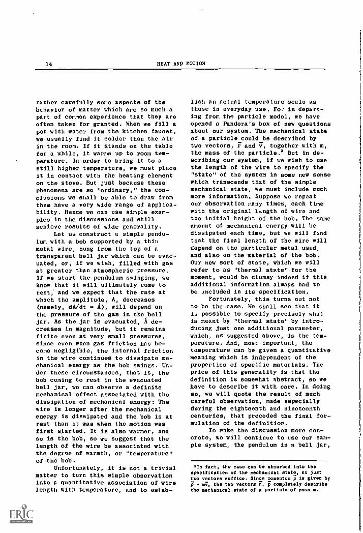
Let us construct a simple pendu-lum with a bob supported by a thinmetal wire, hung from the top of atransparent bell jar which can be evac-uated, or, if we wish, filled with gasat greater than atmospheric pressure.If we start the pendulum swinging, weknow that it will ultimately come torest; and we expect that the rate atwhich the amplitude, A, decreases(namely, dA/dt = A), will depend onthe pressure of the gas in the belljar. As the jar is evacuated, A de-creases in magnitude, but it remainsfinite even at very small pressures,since even when gas friction has be-come negligible, the internal frictionin the wire continues to dissipate me-chanical energy as the bob swings. Un-der these circumstances, that is, thebob coming to rest in the evacuatedbell jar, we can observe a definitemechanical effect associated with thedissipation of mechanical energy: Thewire is longer after the mechanicalenergy is dissipated and the bob is atrest than it was when the motion wasfirst started. It is also warmer, andso is the bob, so we suggest that thelength of the wire be associated withthe degree of warmth, or "temperature"of the bob.

Unfortunately, it is not a trivialmatter to turn this simple observationinto a quantitative association of wirelength with temperature, and to estab-

lish an actual temperature scale asthose in everyday use. Fo' in depart-ing from the particle model, we haveopened a Pandora's box of new questionsabout our system. The mechanical stateof a particlecould_be described bytwo vectors, r and v, together with m,the mass of the particle.3 But in de-scribing our system, if we wish to usethe length of the wire to specify the"state" of the system in some new sensewhich transcends that of the simplemechanical state, we must include muchmore information. Suppose we repeatour observation many times, each timewith the original I.ngth of wire andthe initial height of the bob. The sameamount of mechanical energy will bedissipated each time, but we will findthat the final length of the wire willdepend on the particular metal used,and also on the material of the bob.Our new sort of state, which we willrefer to as "thermal state" for themoment, would be clumsy indeed if thisadditional information always had tobe included in its specification.

Fortunately, this turns out notto be the case. We shall see that itis possible to specify precisely whatis meant by "thermal state" by intro-ducing just one additional parameter,which, as suggested above, is the tem-perature. And, most important, thetemperature can be given a quantitativemeaning which is independent of theproperties of specific materials. Theprice of this generality is that thedefinition is somewhat abstract, so wehave to describe it with care. In doingso, we will quote the result of muchcareful observation, made especiallyduring the eighteenth and nineteenthcenturies, that preceded the final for-mulation of the definition.

To rake the discussion more con-crete, we will continue to use our sam-ple system, the pendulum in a bell jar,

'In fact, the mass can be absorbed into thespecification of the mechanical state, so justtwo vectors suffice. Since momentum p is given by

mv, the two vectors r, F. completely describethe mechanical state of a particle of mass m.

TEMPERATURE AND THERMAL EQUILIBRIUM 15

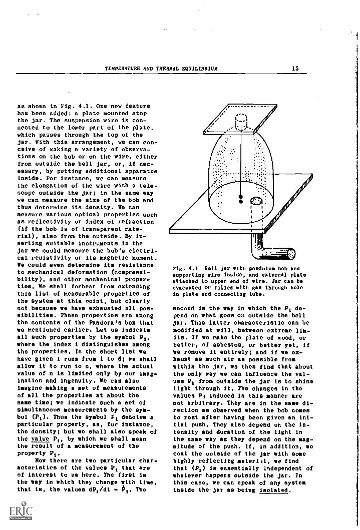
as shown in Fig. 4.1. One new featurehas been added: a plate mounted atopthe jar. The suspension wire is con-nected to the lower part of the plate,which passes through the top of thejar. With this arrangement, we can con-ceive of making a variety of observa-tions on the bob or on the wire, eitherfrom outside the bell jar, or, if nec-essary, by putting additional apparatusinside. For instance, we can measurethe elongation of the wire with a tele-scope outside the jar; in the same waywe can measure the size of the bob andthus determine its density. We canmeasure various optical properties suchas reflectivity or index of reflection(if the bob is of transparent mate-rial), also from the outside. By in-serting suitable instruments in thejar we could measure the bob's electri-cal resistivity or its magnetic moment.We could even determine its resistanceto mechanical deformation (compressi-bility), and other mechanical proper-ties. We shall forbear from extendingthis list of measurable properties ofthe system at this point, but clearlynot because we have exhausted all pos-sibilities. These properties are amongthe contents of the Pandora's box thatwe mentioned earlier. Let us indicateall such properties by the symbol Pi,where the index i distinguishes amongthe properties. In the short list wehave given i runs from 1 to 8; we shallallow it to run to n, where the actualvalue of n is limited only by our imag-ination and ingenuity. We can alsoimagine making a set of measurementsof all the properties at about thesame time; we indicate such a set ofsimultaneous measurements by the sym-bol (Pi). Thus the symbol Pi denotes aparticular property, as, fur instance,the density; but we shall also speak ofthe value Pi, by which we shall meanthe result of a measurement of theproperty Pi.

Now there are two particular char-acteristics of the values Pt that areof interest to us here. The first isthe way in which they change with time,that is, the values dP1 /dt fit. The

Fig. 4.1 Bell jar with pendulum bob andsupporting wire inside, and external plateattached to upper end of wire. Jar can beevacuated or filled with gas through holein plate and connecting tube.

second is the way in which the Pi de-pend on what goes on outside the belljai. This latter characteristic can bemodified at will, between extreme lim-its. If we make the plate of wood, orbetter, of asbestos, or better yet, ifwe remove it entirely; and if we ex-haust as much air as possible fromwithin the jar, we then find that aboutthe only way we can influence the val-ues Pi from outside the jar is to shinelight through it. The changes in thevalues Pi induced in this manner arenot arbitrary. They are in the same di-rection as observed when the bob comesto rest after having been given an ini-tial push. They also depend on the in-tensity and duration of the light inthe same way as they depend on the mag-nitude of the push. If, in addition, wecoat the outside of the jar with somehighly reflecting materiel, we findthat (P1) is essentially independent ofwhatever happens outside the jar. Inthis case, we can speak of any systeminside the-jar as being isolated.

16 HEAT AND MOTION

On the other hand, with a trans-parent jar and air or some other gaswithin it, and a metal plate on top,we find that the values (Pi) willchange measurably if the surroundingschange. Furthermore, they can nowchange in different directions; if wedenote by APi a change in a value Pi,the changes API observed when we putsome ice on the metal plate will ingeneral have signs opposite from theAPI that occur when we put a containerof boiling water on the plate. Underthese circumstances, the system insidethe jar is clearly no longer isolatedfrom its surroundings. But we have inno case done mechanical work on thesystem; we have not, for instance,started it swinging in order to bringabout changes in the vall:es (Pi). Toemphasize this point, we shall speakof "thermal contact" of the system withits surroundings when the changes inthe values (PI) do not depend onchanges in the mechanical state of thesystem or of any part of its sirround-ings.

Now that we have carefully de-scribed the possible thermal relationsbetween a system and its surroundings -from perfect thermal isolation (values(Pi) completely independent of sur-roundings), to varying degrees of ther-mal contact (values (Pi) depending onsurroundings to a lesser or greater ex-tent) - we can consider the other char-acteristics of the values that we men-tioned, namely, their time rates ofchange, Os). The formal statement ofthe behavior of (PI) is quite simple,but some discussion is required to ap-preciate its significance. So first wegive the formal statement:

Under certain special circumstances,each of the values Pi (in the set(Pi) of all the values of propertiesof a system measured at a certaintime), is constant; that is, Pi 8. 0

for all values.

First of all, we should recognise thatthis statement is not true in general,that is, for a system chosen arbitrar-

ily, under unspecified conditions. Ingeneral, we may find that the set ofvalues (Pi) measured at one time willbear no special relation to the setmeasured at another time. Hence theformal statement above is not trivial;the circumstances under which it holdsmust indeed be "special."

We now have to inquire: What arethe special circumstances? What is thesignificance of this statement for thethermal behavior of the system? Theanswer to the first question dependson whether the system we are consider-ing is thermally isolated or in ther-mal contact with its surroundings. Itwe take any system (one which s v ini-tially be in some sort of therm, -.on-

tact with its surroundings), and iso-late it thermally, we find that if wewait long enough, the statement abovewill apply. That is, the values of theproperties will change at rates (Pi)which diminish to zero, and finallyreach a set of values (Pi) which there-after remain constant. Hence one of thespecial circumstances referred to inthe statement is simply thermal isola-tion. Alternatively, if we have a sys-tem in thermr1 contact with its sur-roundings and arrange as carefully aswe can that the surroundings do notchange, then again the statement willapply. From this point on, let us givea name to the condition specified bythe statement, that all values Pi areconstant in time, or all tit - 0; wewill call this condition "thermalequilibrium" and when it is satisfied,we will say that the system is in a"thermal equilibrium state." We candifferentiate among different thermalequilibrium states by the set (Pi) ofconstant values of the properties meas-ured for each such state.

This definition of a thermal equi-librium state is quite precise, butvastly more complicated than the defi-nition of a mechanical equilibriumstate. There, just the two vectors rand p sufficed; here, we need the setof %alues (P1), i 1, 2, . . n,

where there is no obvious limit to thesire of n. The definition of thermal

TEMPERATURE AND THERMAL EQUILIBRIUM 17

equilibrium could clearly have no use-ful role in a theory of thermal proc-esses if it had to remain in this form.But remarkably enough, it is possibleto abstract from this definition justone new parameter, which implicitlycontains the same information regard-ing thermal equilibrium as does theentire set of values (Ps). Let us seehow this can be done, and why this newparameter is associated with the intu-itive notion of temperature.

Our discussion rests on an empiri-cal relation among various thermalequilibrium states, which can be de-scribed in the following way. Supposewe have ascertained that two differentsystems, initially quite independent ofeach other, are each in thermal equi-librium. The systems might each be apendulum in a bell jar as in our ear-lier discussion, or they might be ofentirely different types, not neces-sarily the same for each. Now let usput the two systems in thermal contactwith each other. If the systems eachwere of the type sketched in Fig. 4.1,for instance, this could be done byplacing the bottom plate of one (sys-tem A), on the top plate of the other(system B). Before being placed inthermal contact, they each had theirrespective sets of values (PIA), (Pis).Common experience tells us that afterbeing placed in thermal contact, theywill come to mutual thermal equilib-rium and will then have respective setsof values, (13;A), (Pis), which are ingeneral different from the originalsets of values, before they were placedin thermal contact. Now that they arein mutual thermal equilibrium, theirsets of values have a special property.If we now isolate them we know thattheir respective thermal equilibriumstates will not change; while in isola-tion, the properties retain their re-spective values (PiA), (Pis). Therefore,if we return them to mutual thermalequilibrium, we observe a special kindof behavior, different from what wefind in general: These separated sys-tems, when brought into thermal contact,retain the sets of values (11;1), (10).

which they had before thermal contact.In other words, the values (Pia),

(FIE,), are invariant with respect tomutual thermal contact of systems Aand S. Now these "other words" are notonly more elegant than the original de-scription, they are also more useful.For whenever we find an aspect of aphysical system which is invariant insome context, we can define a new phys-ical quantity in terms of that invari-ance. Mechanics abounds with examples:indeed mass, energy, momentum, etc.,are all useful in describing mechanicalphenomena precisely because each is re-lated to some sort of invariant behav-ior of a mechanical system.

So we have finally arrived (al-most), at the end of our tortuous pathleading to the definition of tempera-ture: Whenever two separated systemsare each in a thermal equilibrium statethat has the property of remaining un-changed after being brought into ther-mal contact, we say that these twostates have the same temperature. It iseasy to see that this definition can beexpanded beyond two states, to includeany number whatever. This can also bedone without bringing all the statesinto mutual thermal equilibrium, forit is also a fact of experience thatif system A and system B are in mutualthermal equilibrium (hava the sametemperature), and A is also separatelyin thermal equilibrium with system C,then B will be found to be in thermalequilibrium with C if they are placedin mutual thermal contact. Thus A, 13,C all have the same temperature, sothis can be established for any numberof systems by observing their behaviorin mutual thermal equilibrium, pair bypair.

We will describe in the next sec-tion how this property of systems inmutual thermal equilibrium, their com-mon temperature, can be given a quan-titative form. That is, we will showhow to assign a number, which we willdenote T, to represent the temperatureof a thermal equilibrium state. Assum-ing for the moment that we have al-ready done this, we now have another

18 HE AT AND MOT ION

value to add to the set (Pi) associatedwith each thermal equilibrium state.But this number T is not on ah equalU)oting with all the rest in the set(Pi), for it completely specifies thethermal equilibrium state, in a waywhich is not shared by any of the othervalues.

In order to see the meaning ofthis statement, that the temperaturehas a special significance which dis-tinguishes it from the other propertiesof a system, let us return to the oper-ation we consIdered in defining thetemperature. We brought two systems,initially separated and each in ther-mal equilibrium, into thermal contact,and used the outcome of this operationto define temperature. Now let us con-sider instead the converse question;We know the initial values of the prop-erties in thermal equilibrium, (P )--1AJ(Pie), and we would like to predict theoutcome. But our Pandora's box con-tained a large number of propertiesthat can be defined for any particularsystem, and an enormous number of dif-ferent conceivable systems. As a re-sult, making even this simple predic-tion becomes a major task.

In special cases, the answer issimple. For instance, if the two sys-tems are the same, and if just one ofthe properties, say the density, hasdifferent initial values, then theywill not be in mutual thermal equilib-rium when brought into thermal contact;their values of all their propertieswill change and ultimately they willeach arrive at new thermal equilibriumstates. But if the two systems are dif-ferent, or if two systems of the samekind have different initial values forseveral of their properties, we cannotmake a prediction so easily. Either re-sult possible, depending on the par-ticular set of initial values (PIA),(Pip). We could make the prediction ifwe had made the identical observationbefore, or if we had made a whole se-ries of observations, so that we couldrelate tll the different values of eachPi which are found in different thermalequilibrium states.

But all this complex ty is reducedto trivial simplicity if v.e rememberthe lefinition of temperature. No twodistinct thermal equilibrium stateshave the same temperature, even thoughthey may share common values of otherproperties. For instance, we may finethe same density in states correspond..ing to different temperatures. Con-versely, we may find different densi-ties in states corresponding to thesame temperature. So our predictioncan be made solely on the basis ofwhether or not TA TA before the sys-tems are brought into thermal contact.We need not inquire at all into thevalues of any of the other properties.It is in this sense that temperature,T, defines a thermal equilibrium statecompletely, and implicitly conveys in-formation also contained in the entireset of values (Pi).

4.2 TEMPERATURE SCALES.

In the last section, we defined"temperature" abstractly, as the com-mon property of all systems in mutualthermal equilibrium. But this defini-tion does not suffice to establish tem-perature scale. In order to define atemperature scale, we need a definiteprocedure for assigning, to each setof thermal equilibrium states in mutualthermal equilibrium, a number to rep-resent T. Such a quantitative scale isneeded in all applications of the no-tion of temperature, for instance, inthe mundane task of reporting theweather. (What is the "system" in thiscase?) However, our interest in dis-cussing how to establish a temperaturescale goes beyond a concern with prac-tical applications. We recall that weset ourselves the task of bridging thegap between mechanical and thermal phe-nomena by incorporating both in a con-sistent and coherent model of nature.We were led to our abstract definitionof temperature while working at thistask. The problem we face now is atypical one, which arises whenever anabstract definition must be given a

TEMPERATURE AND THERMAL EQUILIBRIUM 19

concrete form. In the case of tempera-ture, tit. problem is especially com-plex, since our definition was couchedin a particularly abstract and mathe-matical form.

We might ask, however, was thisapproach, from the abstract to the con-crete, really wise? Might it not havebeen better to go in the opposite di-rection, from concrete examples of tem-perature scales to an abstract defini-tion of temperature based on theseconcrete examples? Actually, in pro-ceeding as we did, we were relying onan intuitive feeling for the idea oftemperature. The abstract definitioncould scarcely have any meaning at allfor a reader with no experience withthermometers, or with the sensationsof "hot" and "cold." What we would liketo avoid in our discussion is exclusivereliance on sensation in deciding whatwe mean by "hotter" and "colder." Itis well known how unreliable suchjudgments can be. For instance, if aperson places one hand in very hotwater and the other in ice water, thesensations in the two hands will bevery different when both are put intoa pan of lukewarm water. But even ifwe can avoid such confusion, we wouldlike to be able to describe our modelof nature in a way that is independentof human physiology.

However, we cannot simply side-step the notions "hotter" and "colder,"since they are central to the problemof establishing a temperature scale.In fact, the abstract definition oftemperature given in the last sectionis really incomplete, precisely be-cause it has no reference at all tothese notions. What we must do is togive meaning to these ideas on thebasis of physical phenomena, withoutinvoking human sensations. In doing so,we will not only see how to establishtemperature scales, but also to makeour abstract definition of temperaturemore complete.

For guidance in how to proceed,let us examine how another scale, saythat of mass, may be set up. The massof a certain object is arbitrarily

taken as the unit, and of course dif-ferent choices of the unit lead to dif-ferent scales. For any specific choiceof a unit, the mass of any other objectcan be compared with that of the unitby placing them on opposite pans of anequal-arm balance. The descending armof the balance then contains the "heav-ier," or more massive, object. Thechoice of associating "descending arm"(rather than "ascending arm"), withlarger mass is not really arbitrary,nor does it depend on physiology, al-though it would agree with the choicemade by hefting the two objects. It de-pends on the statement that two identi-cal objects, taken together, have twicethe mass of one of them alone.

The exactly analogous procedureis not possible with temperature, un-fortunately, since there is no proced-ure for adding two temperatures thatcorresponds to the simple addition oftwo masses, and consequently, thechoice of a particular object as a"unit" is impossible. Instead, we canchoose a particular thermal equilibriumstate of some ctnvenient system as a"standard state"; we will call thissystem a "thermometer." We can thenuse the value of a specified propertyof the thermometer in the standardstate (we will call this the "thermo-metric property"), to fix the onepoint of the temperature scale. Thevalues of the thermometric propertywhen the system is in other thermalequilibrium states, compared with itsvalue for the standard state, thengive numbers that represent the tem-perature in these other states. Now wecan put the thermometer in thermal con-tact with any other system, say ourpendulum bob. When the two systemshave come into mutual thermal equilib-rium, we can assign to the equilibriumstate of the bob the temperature asso-ciated with the corresponding equilib-rium state of the t!.,Aometer.

Now we can ask whether the newthermal equilibrium state is hotter orcolder than the standard state. We cangive an unequivocal anewer bl observingwhat happens when mechanical energy is

20 HEAT AND MOTION

dissipated in a system: if its tempera-ture changes at all, it always getshotter, never colder. This statementholds for all systems, regardless ofthe way in which mechanical energy isdissipated: rubbing friction in solids,stirring (viscous friction), in fluids,dissipation of electrical energy whencurrents flow; it is one of the widestgeneralizations that can be made fromexperience. It can also be put intoanalytical form, whereupon it becomesthe basis for a powerful tool in dis-cussing thermal phenomena, namely thesecond law of thermodynamics. Here,however, we use it only to connect thenotions "hotter" and "colder" to tem-perature scales. To make this connec-tion explicit, let us denote the tem-perature of the standard state by thenumber T8, and that of some other stateby f'. Then of the two transitions be-tween these two states, T8 to T' or T'to T8, it is possible to achieve onlyone by dissipating mechanical energyin the system. The one that is possi-ble defines the beginning temperatureas "colder," the final temperature asOa "hotter" of the two. Suppose weffad in this way that, say, To iscolder than a particular temperatureT1, and hotter than another tempera-ture T8. Then we will always find thatit is impossible to go from T1 to Toby dissipating mechanical energy; thatis, we will always find that T1 is hot-ter than TE.

Notice that we have said nothingyet about a relation between the mag-nitudes, or algebraic values, of thenumbers we have assigned to representthe temperatures of various thermalequilibrium states. Although we havedecided unequivocally that the statelabeled T1 is hotter than the state la-beled TI, this does not automaticallyimply that the number T1 is larger thanthe number Tt. In fact, one of theearliest tem,erature scales assignedthe number 0 to the equilibrium stateof boiling water, and the number 100to that of ice. The opposite conven-tion is now universal; all temperaturescales we use assign numbers in such a

way that they increase alge)raically aswe go from colder thermal equilibriumstates to hotter. Hence all states withnumbers smaller than that assigned tothe standard state are colder than anystate with a number larger than that-of the standard state. If the standardstate is assigned to the number zero,this means that all states with nega-tive temperatures are colder than anystate with a positive temperature. Butthis statement also is merely a matterof convention, since the choice ofstandard state is arbitrary. One ofthe temperature scales we discuss be-low, the "gas-thermometer" scale, re-moves this arbitrariness to some ex-tent, since it assigns the temperature"zero" in a way that appears to benatural and inevitable.4

Now that we have given the mean-ing of "hotter" and "colder" a physi-cal basis, we can return to our de-scription of how a temperature scaleis set Jp. We recall that we start witha particular system to serve as a ther-mometer, this choice corresponding tothe selection of a particular objectas the unit of mass, in the prepara-tion of a scale for mass. Just as thechoice of a particular object for theunit of mass is essentially arbitrary,being limited only by questions oftechnical convenience, so also is thechoice of a particular thermometer.Different applicatioas impose differenttechnical considerations, so there isa great variety of thermometers in ac-tual use. One of the most common isthe liquid-in-glass type. A small massof liquid, commonly mercury or coloredalcohol, is contained in a bulb at-tached to a capillary tube. This sys-tem is the thermometer, and the densityof the liquid (or its volume, inversely

4This aspect of the bas - thermometer scale, whichleads to interesting and useful significance for

the label 0, and even for negative tempera-tures, is discussed in Appendix 3. However,reading this appendix should be deferred untilthe present sect!** is completed, since the ap-peadia osmoses fasillority with the descriptionof the gas-thersoseter scale which is givesbelow.

TEMPERATURE AND THERMAL EQUILIBRIUM 21

related to the density), is the ther-mometric property. Fahrenheit, in theeighteenth century, was one of thefirst to use a thermometer of thissort, and he chose a freezing mixtureof salt and water as the standardstate. The relative volumes of bulband capillary tube are chosen so thatwhen such a thermometer is in equilib-rium with the standard state, most ofthe liquid will be in the bulb, butsome will be in the capillary tube.The origin of the temperature scale isfixed by assigning the number zero asthe temperature of all systems in ther-mal equilibrium with this particularstate. In other thermal equilibriumstates, since the density of the liq-uid will be larger or smaller, smalleror larger amounts of the liquid willbe in the capillary tube. When thethermometer is in equilibrium with thebody of an "average" adult, the densityof the liquid is lower, its volumelarger, and so the length of capillaryoccupied will be larger. Fahrenheit as-signed the number 100 to the tempera-ture of this new equilibrium state,and any other state can then be as-signed a number corresponding to thelength of capillary occupied by liquidwhen the thermometer is in equilibriumwith the chosen state. When the ther-mometer is in equilibrium with a mix-ture of water and ice which itself isin thermal equilibrium, 32% of thelength between the zero and 100 marksis filled, so the temperature is 32"degrees Fahrenheit" (0F). In a simi-lar manner, the temperature of waterin equilibrium with steam at atmos-pheric pressure is found to be 212°F.Clearly, this thermometer cannot beused at temperatures so llw that theliquid freezes, or so high that it va-porizes.

The temperature scale determinedby such a thermometer will depend onthe particular liquid used, and altoon the material of the bulb and capil-lary, since densities of different ma-terials vary in different ways overthe range of temperature in which thethermometer is used. A system in which

the thermometric property did Sot de-pend on the particular substance makingup the system would clearly provide thepossibility of constructing a superiorthermometer. But whether or not such asystem exists is not a matter of defi-nition or logic. It is purely an empir-ical question, to be decided by experi-ment. However, the results of experi-ment, namely that a thermometer doesexist which is largely independent ofthe particular substance used, has in-teresting consequences for our modelof thermal phenomena. We shall exploresome of these consequences in latersections, but first we will describeone such thermometer, the constant-volume gas thermometer.

If a mass of gas, which we denotem, is enclosed in a fixed volume V,,its pressure, P, is found to be dif-ferent in different thermal equilibriumstates. The pressure can then be usedas a thermometric prcrierty, and thenumerical value of temperature, whichwe will denote To, can be assigned ac-cording to a rule analogous to thatused with the liquid-in-glass thermom-eter. There the numerical value of tem-perature was associated with the lengthof liquid in the capillary, as comparedwith the length when the thermometerwas in the standard state. Here we usea somewhat different standard state,

namely that in which water, water va-por, and ice are in mutual thermalequilibrium. The pressure of the gasis found to have a reproducible value,which we denote Po, when its containeris in thermal equilibrium with thestandard state, and the temperature ofthe standard state is defined as Tc0. The temperature, Te, in any otherthermal equilibrium state is then de-fined in terms of the ratio P(T)/Flo bythe equation

F(Te)/P0 1 + aTe 6. 1 4 TO /To, (4.1)

where in tha last equality we have sim-ply written Vro for the constant, a.This constant determines 'ht size ofthe unit temperature difference, or"degree." In the common Celsius scale

22 HEAT AND MOTION

(formerly called the centigrade scale),it is fixed by setting the temperatureof the "steam point" (water in equilib-rium with its vapor at standard atmos-pheric pressure), as equal to 100 de-grees Celsiva (°C). Therefore, if themeasured pressure at the steam pointis P(100),

P(100)/130 - 1 + 100 a,

a - [P(100)/P0 - 1] /100 - 1/To

(4.2)

Therefore, Eq. (4.1) can be written

To/To P(To)/P0 - 1. (4.3)

This equation is not quite symmetrical,because of the -1 on the right-handside. A simple algebraic trick can con-vert the equation into a more symmet-rical form, in terms of a new tempera-ture scale which differs from that inEq. (4.3) only by changing the origin,that is, the state which is denoted"zero degrees," but leaving the size ofthe degree unchanged. If the term -1is transposed,

P(T ) . a (To + To) IL.

Po To To To.

Tr Tc Tr. (4.4)

We will call the temperaturescale denoted by TR, and defined bythe last equality in Eq. (4.4), the"gas thermometer scale." This is not auniversal scale, since it does dependto some extent on the particular kindof gas in the volume V. Suppose weplace several such thermometers, eachcontaining a different kind of gas, inmutual thermal equilibrium, after hav-ing prepared each with the same pres-sure Po in the standard state. We willfind, in general, that each thermome-ter will have a slightly differentpressure when they are all in a thermalequilibrium state which is differentfrom the standard state. That is, ifwe write Eq. (4.4) as

Tg [P(Tg) /Po]To, (4.5)

we find that P(Tg) is slightly dif-ferent for each gas. Since accordingto our definition of temperature, Tgis the same for all thermometers, thismeans that To must have a slightly dif-ferent value for each gas. Now we canimagine repeating the same procedure,each time starting with a lower valueof Po in the standard state (either byusing less gas in the same volumeor larger V. with the same m, or both),and then returning to the state idmi-tified by Tg. As Po is decreased,value of P(Tg) is naturally found todecrease as well. But we will also findthe important result that the differ-ences in P(Tg) for the different gasesbecome smaller and smaller. That is,as Po decreases, the ratio P(Tg)/P0approaches a constant value which isindependent of the gas in the thermom-eter. If the same procedure is carriedout for other thermal equilibriumstates, that is, with different valuesof T1. the same effect is observed.The ratio P(Tg)/P0 again approaches alimiting value (as Po approaches zero),which is again independent of the gasused. This limiting value depends ontemperature Tg, but in a very simplefashion: It is proportional to Tg.Hence under these conditions (limit oflow pressure), To is a constant whichis the same for all gases, and at alltemperatures. We have been quoting theresults of extensive experimental in-vestigation carried out at the end ofthe seventeenth century by Boyle, Mari-otte, Charles, Gay-Lussac and others,and considerably refined since then.The best current value of To, deter-mined by the procedure described above,is

To 1- 273.16 degrees.

Thus in the limit of low pressure,Eq. (CS) becomes the definition of atemperature scale which is independentof the substance used, although itstill refers to a particular system,an enclosure filled with gas. We will

TEMPERATURE AND THERMAL EQUILIBRIUM 23

refer to this scale as the "ideal gas"scale.

We will not digress to discuss ingeneral the question of hog tempera-tures are measured in practice whenhigh precision and accuracy are re-quired. One aspect of this problem,the intercomparison of temperaturesscales associated with different kindsof thermometers, is discussed brieflyin Appendix 4. In later sections, wewill return to a discussion of the

ideal gas temperature scale whichwill give us further insight into theconnection between mechanical anthermal phenomena. At this point, wecan already see one such relation.The ideal gas scale distinguishesamong different thermal states, usingonly the purely mechanical procedureof measuring pressures, and withoutrequiring any information about anyproperties of specific substances.

5 DO THERMAL EQUILIBRIUM STATES EXIST?

From the point of view of our mainline of discussion, our description oftemperature scales in the last sectionwas a long digression, but it was in-tended to serve a definite purpose. Inthe previous section, we stated thedefinition of thermal equilibrium in apurposely abstract form in order tomake it clear that this definition isgenerally valid, without reference tospecific properties of particular sub-stances. But a price must be paid forsuch an abstract treatment: It makesthe concept described remote from ex-perience, and it becomes difficult toconnect the abstract idea with concretereality. The discussion in the lastsection was intended to close this gapby showing that thermal equilibrium,and the concept of temperature whichit defines, have a perfectly definitemeaning. Furthermore, we saw that thismeaning could be described in toms ofsimple operations carried out on realobjects. Having completed that discus-sion, we can return now to a furtherexamination of thermal equilibrium witha clearer idea of the physical proc-esses involved.

Notice that thermal equilibriumdiffers from mechanical equilibrium ina rather important respect. A systemin a thermal equilibrium state remainsin that state as long as it is iso-lated, or, if it is in contact withits surroundings, as long as its sur-roundings do not change. In the me-chanical model, there is nothingstrictly comparable to this property.Mechanical equilibrium requires onlythat the velocity v const, so that aparticle in equilibrium passes throughan infinite number of positions in suc-cession, and hence through an infinityof different mechanical states. Onespecial mechanical equilibrium state,that for which v 0, and thereforer const, (particle at rest), mightseem analogous to the thermal equilib-

24

rium state, since a particle at restdoes not pass through other mechanicalequilibrium states in the course oftime. However, the particular mechani-cal equilibrium state corresponding toa particle at rest does not reallyhave any special significance. As amatter of fact, this lack of signifi-cance for the "rest" state is no acci-dent, but a fundamental feature of me-chanics. It arises from the fact thatall frames of reference, which differonly by virtue of a constant relativevelocity between their origins, areprecisely equivalent in the mechanicalmodel, Therefore, if a particle is atrest in one reference frame, there ex-ists an infinity of completely equiva-lent reference frames, each movingwith respect to the first with a con-stant velocity, with respect to whichthe particle is still in equilibrium,but no longer at rest.

We can make thin relation betweenequivalent reference frames more ex-plicit by referring again to Fig. 2.1.The two reference frames in the figureare distinguished from each other bythe two origins, 01 and Os. In ourearlier discussion, the vector joiningthe two origins was a constant,In our present discussion, this vectoris a function of time, since the tworeference frames are moving with re-spect to each other. Since their rela-tive velocity is a constant vector,which we can denote V, we can write

Rai (t) 1121(0) + Vt, (5.1)

where gs(0) is also a constant vec-tor. Now suppose 0, is the origin ofthe reference frame in which the par-ticle is at rest. Then v, 0, and,taking the time derivative of bothsides of Eq. (2.1), with Eq. (5.1) forRai, we have

V.

DO THERMAL EQUILIBRIUM STATES EXIST? 25

Hence, while the particle is not atrest in the reference frame whose, ori-gin is 02, since v2 is not zero, it isstill in equilibrium in that frame,since V is a constant vector.

It is worth recognizing that thesetwo different kinds of specificationfor equilibrium (a stable state withfixed parameters in the thermal case,a succession of different states, re-lated by Eqs. (2.6) and (2.7) in themechanical case), both come from thesame kind of abstraction from naturalphenomena. The principle of abstrac-tion which is common to both is therecognition, in each case, of the fun-damental characteristic of a disturb-ance. For a particle, a disturbancedoes not involve merely a change inposition, but rather a change in ve-locity; this is the basic statement ofN-II. For a thermal system, on theotb hand, any change of its parame-terb whatever is caused by a disturb-ance, so thermal equilibrium is repre-sented by a stable state.

This stability of thermal equilib-rium states, in the absence of disturb-ance, leads immediately to the specifi-cation of a unique direction of timewithout any reference to mechanicaleffects. We recall our description ofmutual thermal equilibrium: two iso-lated thermal systems, each in thermalequilibrium, but at different tempera-tures, are placed in thermal contactwith each other, while still isolatedfrom any other surroundings. In time(at a rate which depends on their de-gree of thermal contact), they eachreach a new equilibrium state, andthese two final states have the sametemperature, which is between the twoinitial temperatures. Now if we watchedthis process in reverse, we would seean isolated system, with two parts inmutual thermal equilibrium, as theinitial state. This is a differentinitial condition than we consideredpreviously, and we recall that when wediscussed time reversal in mechanicalsystems, we saw that changing the di-rection of time also changed the ini-tial mechanical state, since the veloc-

ity was reversed. But in th) case ofthe motion of particles, the behaviorafter time reversal was still a possi-ble motion, even though it was not ex-actly the same as that which precededtime reversal. In the present case,however, when we consider the behaviorof our thermal systems, we see thatthis is no longer the case. The proc-ess as observed with time reversedwould show us the two systems, origi-nally in mutual thermal equilibrium,changing their temperatures in oppo-site directions, one getting coolerand one warmer, while thermal contactwas still maintained, although theyhad no contact, mechanical or thermal,with any surroundings but each other.This process, which would be observedafter time reversal, is never observedin nature. Two systems, once in mutualthermal equilibrium, are always ob-served to maintain that condition aslong as they are isolated from anyother surroundings. Hence the directionof time, in which the "disequilibrium"process would be described, is thewrong direction, and is so recognizedwith no reference to any mechanicaleffects such as dissipation of mechan-ical energy, which we used earlier tospecify the "correct" direction oftime flow.

5.1 FLUCTUATIONS IN THERMALPROPERTIES.

If this were an entirely accuratedescription of what can and cannot beobserved when we examine the approachto thermal equilibrium, nature wouldbe very different in certain fundamen-tal respects. Just what these differ-ences might be, we will discuss later.Pt the moment, we can remark that thecescription given above of the approachto thermal equilibrium is fairly accu-rate, sad can serve as a first approxi-mation to the true situation. However,the details which it ignores are justas important to a complete understand-ing of the process as those which wereincluded. Let us go beyond this glib

26 HEAT AND MOTION

description and examine some of thesemissing details.

When we look at the approach tothermal equilibrium in further detail,we will be led to the conclusion that,strictly speaking, thermal equilibriumcan never be observed. In section 4.1,thermal equilibrium was defined by thecondition (f'' 0) for all measured val-ues of all properties of a system. Aswe shall see, this condition can neverbe satisfied precisely, but for twodifferent kinds of reasons. We willnow examine these two reasons in turn.

In general, if we examine somethermal system at a particular instant,at which we arbitrarily set t 0, itwill not be in a thermal equilibriumstate. If at that instant we thermallyisolate the system from its surround-ings, or, alternatively, if we fix theconditions of the surroundings so theyremain the same as they were at theinitial instant, t 0, the system willapproach some final thermal equilibriumstate. We expect this approach to besmooth, or continuous, in the mathe-matical sense. We.also expect that therates of change (Pi) will decrease inmagnitude as the (Pi) approach theirfinal values, which we will denote(Pi(°4). Both of these conditions canbe satisfied in the following way. Wedefine a quantity 0i(t) as the differ-ence between the final value of Pi andthe value of Pi at time t:

0i(t) Pi(o) - Pi(t). (5.2)

If this quantity is positive, then attime t, Pi is smaller than its finalvalue, so at time t, Pi must be in-creasing; hence Pi(t) is also positive.Conversely, if APi(t) is negative, thenPi is also rngatil,e. The simplest wayof ensuring that Pi(t) decreases inmagnitude as Pi(t) approaches its equi-librium value is to set this time de-rivative proportional to the differenceremaining at time t, that is, to01(t). If we choose a proportionalityconstant which has the dimensions oftime, and denote it r, we can write

0i(t)/r. (5.3)

We should point out that we have not"proved" that the (Pi) and their timederivatives must satisfy this equation;we have simply shown that if they do,they will satisfy the two expectationsstated at the beginning of this para-graph. Therefore, Eq. (5.3) shouldprovide at least an approximate de-scription of the actual approach tothermal equilibrium.

Equation (5.3) has a form whichis found to apply to a great varietyof physical problems, since the condi-tions suggested at the beginning ofthe last paragraph, which led us topostulate this equation (not "derive"it), are reasonable expectations inmany different physical situations.Radioactive decay is one of these sit-uations; it also governs the approachto terminal speed of a particle fallingin a resietive medium, in certain cir-cumstances. In this last context, itwas discussed in Appendix 1, where itwas shown how a solution can be de-rived. Here we will simply state thesolution, and show that the statementis correct by calculating the time de-rivative, and comparing the resultwith Eq. (5.3). We assert

01(0 01(0) a -t/r. (5.4)

where e is the base of natural loga-rithms. Taking the time derivative ofboth sides,

4)i(t)- 1 Ap (0) - 01(07 e

(5.5)

where we have used Eqs. (5.3) and (5.2)in making substitutions. Hence, we seethat the time derivative of Eq. (5.4)does agree with F1. (5.3), so we haveindeed found a solution to the latterequation. We will call this solutionthe equation of "exponential relaxa-tion" becarse of the exponential fac-tor, and refer to r as the 'relaxationtime."

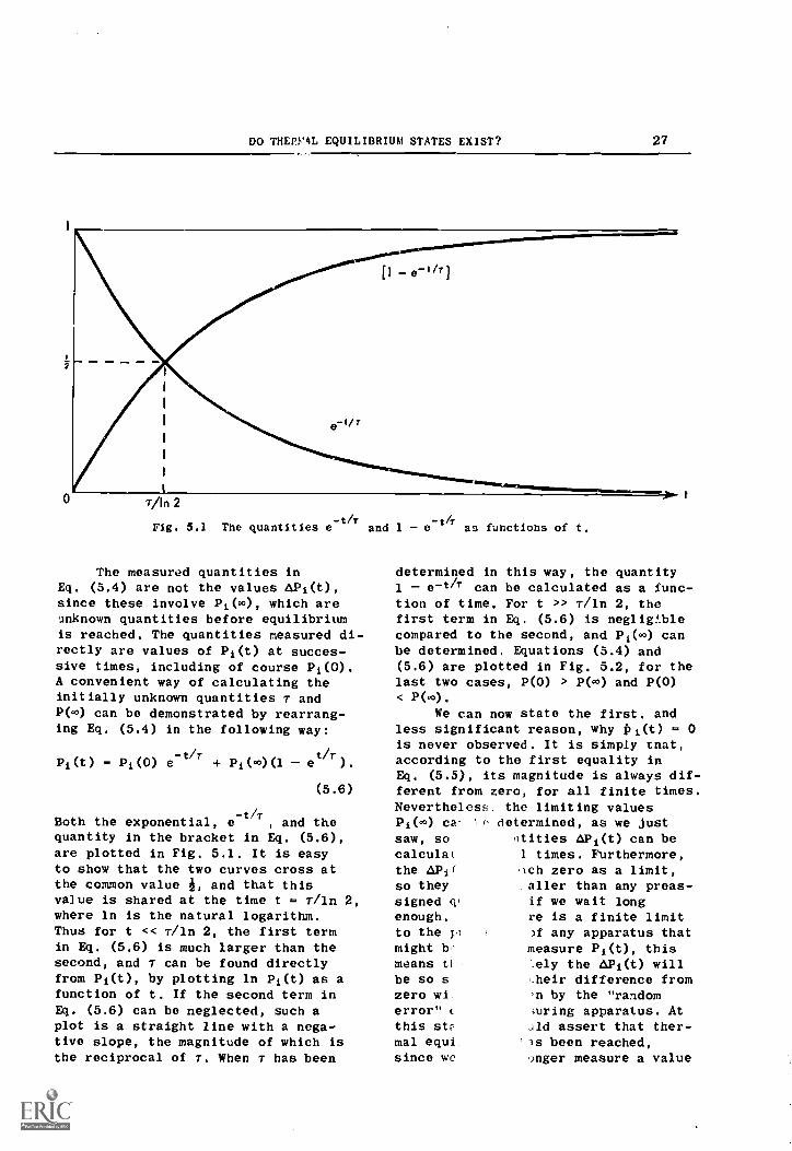
DO THERV4L EQUILIBRIUM STATES EXIST? 27

[1 - e- /7 )

Tiln 2

Fig. 5,1 The quantities e-t/r

and 1 e-t/T

as functions of t.

The measured quantities inEq. (5.4) are not the values AP1(t),since these involve Pi(w), which are.unknown quantities before equilibriumis reached. The quantities measured di-rectly are values of Pi(t) at succes-sive times, including of course Pi(0).A convenient way of calculating theinitially unknown quantities T andP(.0) can be demonstrated by rearrang-ing Eq, (5.4) in the following way:

Pi(t) = Pi (0) e-t/r

+ Pi(0)(1 et/r

).

(5.6)

Both the exponential, a -t /T, and thequantity in the bracket in Eq. (5.6),are plotted in Fig. 5.1. It is easyto show that the two curves cross atthe common value and that thisvalue is shared at the time t = T/ln 2,where ln is the natural logarithm.Thus for t << T/ln 2, the first termin Eq. (5.6) is much larger than thesecond, and T can be found directlyfrom Pi(t), by plotting ln Pi(t) as afunction of t. If the second term inEq. (5,6) can be neglected, such aplot is a straight line with a nega-tive slope, the magnitude of which isthe reciprocal of T. When T has been

determined in this way, the quantity1 e-t/r can be calculated as a func-tion of time. For t >> r/ln 2, thefirst term in Eq. (5.6) is neglig:thlecompared to the second, and Pi(w) canbe determined. Equations (5.4) and(5.6) are plotted in Fig. 5.2, for thelast two cases, P(0) > P(.0) and P(0)< P(.0),

We can now state the first, andless significant reason, why Pi(t) = 0is never observed. It is simply tnat,according to the first equality inEq. (5.5), its magnitude is always dif-ferent from zero, for all finite times.NeverthelesE, the limiting valuesPi(w) ca' 10 determined, as we just

'titles API(t) can be1 times. Furthermore,ich zero as a limit,ialler than any preas-if we wait longre is a finite limit

any apparatus thatmeasure Pi(t), thisely the APi(t) will.heir difference fromn by the "random,uring apparatus. AtJld assert that ther-

'is been reached,anger measure a value

saw, socalculatthe APOso theysigned qienough.to the pl

might bcmeans tibe so szeroerror" cthis strmal equisince we

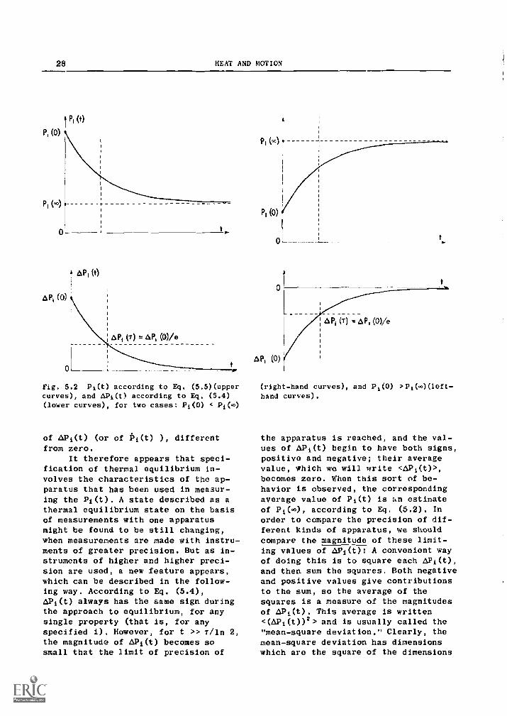
28 HEAT AND NOTION

P, (0)

Pi

0

Pi (t)

t

1 aP, (t)

AP, (0)

0

41,i (7) = AP, (0)/e

Fig. 5.2 Pi(t) according to Eq. (5.5)(uppercurves), and APi(t) according to Eq. (5.4)(lower curves), for two cases: Pi(0) < Pi(m)

of APt(t) (or of Pi(t) ), differentfrom zero.

It therefore appears that speci-fication of thermal equilibrium in-volves the characteristics of the ap-paratus that has been used in measur-ing the PIM, A state described as athermal equilibrium state on the basisof measurements with one apparatusmight be found to be still changing,when measurements are made with instru-ments of greater precision. But as in-struments of higher and higher preci-sion are used, a new feature appears,which can be described in the follow-ing way. According to Eq. (5.4),APi(t) always has the same sign duringthe approach to equilibrium, for anysingle property (that is, for anyspecified i). However, for t >> 7/1n 2,the magnitude of API(t) becomes sosmall that the limit of precision of

PI (0)

0

API (0)

t.

(right-hand curves), and Pi(0) >Pi(m))(left-

hand curves).

the apparatus is reached, and the val-ues of APi(t) begin to have both signs,positive and negative; their averagevalue, which we will write <AP1(t) >,becomes zero. When this sort of be-havior is observed, the correspondingaverage value of Pi(t) is an estimateof Pi(.0), according to Eq. (5.2). Inorder to compare the precision of dif-ferent kinds of apparatus, we shouldcompare the magnitude of these limit-ing values of APi(t): A convenient wayof doing this is to square each A,101(t),and then sum the squares, Both negativeand positive values give contributionsto the sum, so the average of thesquares is a measure of the magnitudesof APi(t). This average is written<(6,Pi(t))2> and is usually called the"mean-square deviation." Clearly, themean-square deviation has dimensionswhich are the square of the dimensions

DO THERMAL EQUILIBRIUM STATES EXIST? 29

of the corresponding Pi. If we takethe square root of the mean square de-viation, we obtain a quantity which iscalled the "root-mean-square devia-tion," which we will denote (aPi)rins or

u(APi). The root-mean-square (or"rms"), deviation is a measure of themagnitudes APi(t) which, as we see,has the same dimensions as Pi itself.For later reference, we write the for-mal definition:

cr(APi) (APOrms -1/<(A.P1)2>

= E (6,131)di (5.7)j=t

where, in the last equation, we havewritten out the average explicitly: Ndifferent measurements of Pi(t) havebeen included, each giving a value of(AP1)2; these values have been labeledwith the index j, which runs from 1 toN. From our discussion above, we seethat o(A.P1) may serve as a measure ofthe precision of the instrument usedin the measuring Pi(t); the greaterthe precision, the smaller we wouldexpect cr(APi) to be.

Although the result of this longdiscussion, leading to the definitionof the rms deviation er(AP1), allows usto compare the precision of differentkinds of measuring apparatus, this isnot the primary reason for definingcr(APi). Our main motivation was thatcertain very important characteristicsof a series of measurements of Pi(t),made for t >> T/ln 2, can be statedsuccinctly in terms of that definition.These characteristics are:

(a) If measurements of greater andgreater precision are made, it isfound that cr(APi) does not decreaseindefinitely; a lower limit tocr(aPi) is reached, and the rms de-viation does not decrease belowthis lower limit, regardless of theprecision of the measuring appa-ratus.

(b) This lower limit to a(6,Pi),while it is independent of the

measuring apparatus, does depend onthe system whose values of Pi(t)are being measured, and in two ways:

(i) The (noninstrumental) lowerlimit to v(APi) in general in-creases as the size of the sys-tem decreases;

(ii) It also increases withhigher terhperature.

We shall refer to deviations APi(t)which are observed when this lowerlimit to (TWO has ben reached, sothat properties of the measuring appa-ratus are irrelevant, as fluctuationsof the system. What we have statedabove, then, are properties of fluctu-ations observed, at least in princi-ple, in all thermal systems.

The qualification, "in princi-ple," must be made because of thestatement labeled (b),(i) above. Forsufficiently large systems, the fluc-tuations become so small that the non-instrumental limit to cr(APi) is neverreached. Hence the deviations APi(t)that are observed, are related to themeasuring apparatus, and are not aprc:derty of the system, and thereforeare not fluctuations as defined above.This circumstance makes it possible toavoid fluctuations in practice, simplyby increasing the size of the system,or of the surroundings with which thesystem is in thermal contact. For in-stance, if we wished to avoid tempera-ture fluctuations of a pendulum bob inan arrangement such as that illustratedin Fig. 4.1, we would place a very mas-sive object, which itself was in ther-mal equilibrium, on the upper plate.In actual practice, the bob would beplaced directly in a large mass of liq-uid, since the best thermal contactwould be achieved this way. Boiling anegg is a familiar example of this pro-cedure. Because of the wide range oftemperatures over which different liq-uids condense, "temperature baths" arenot limited to the ordinary tempera-tures we commonly experience. The low-est temperature that can be reached inthis way is about 0.3°K above the ab-

30 HEAT AND MOTION

solute zero, the liquid for this bathbeing the rare isotope of helium, He3,boiling under reduced pressure.

We can now answer the questionposed earlier, "Do thermal equilibriumstates exist?" According to the defini-tion in section 4.1, the answer mustbe "No," because of the presence offluctuations. But it is much more rea-sonable to base definitions on physi-cal grounds, so a preferable answer is"Yes," with the understanding that theconditions Pi 0, or APi = 0, are notsatisfied exactly, because of the ex-istence of fluctuations. The possibil-ity of observing fluctuations is thusincorporated into an expanded defini-tion of thermal equilibrium. The con-clusions that we can draw from this ex-tended definition, about the internalconstitution of matter, are explored inthe next section.

Before proceeding to this discus-sion, we should consider two pointswhich have so far been neglected, whoseclarification will help us later on.In the first place, even with our def-inition of thermal equilibrium ex-tended so as to include fluctuations,there is still a sense in which thermalequilibrium states do not exist. Sup-pose we consider a system in thermalisolation, which has come to thermalequilibrium in the extended sense, sothat the Pi are exhibiting fluctuationsabout their average values, Pi(m). Nowperfect thermal isolation is an ideal-ization from experience, and can neverbe achieved in practice. Therefore, ifthe temperature T(m) of the isolatedsystem is different from that of thesurroundings, say T', there will be aslow variation of T(m) toward T'. Thisvariation may be approximated byEqs. (5.4) or (5.6), but with a relaxa-tion time which is long compared tothe relaxation time T, which gave therate at which the isolated system ap-proached T(m). Hence in order to ob-serve the equilibrium of the isolatedsystem, we must wait until t >>7/1;), 2,but we must not wait so long thatt r'/ln 2.

The same sort of "superposition"

of thermal equilibrium stags, with re-laxation times of very different size,is found in most physical systems. Forinstance, objects that are made ofmetal that has been deformed by forg-ing, stamping, etc., during manufac-ture, will exhibit very slow changes insize and shape in the course of time.On a different scale of size, galaxiesevolve at rat,ls which are very slow ona human time scale. A small portion ofa galaxy may therefore appear to be inequilibrium at any instant, despiteits slow change to a new state.

In general, therefore, thermalequilibrium states as observed in phys-ical systems are not likely to be trulystable; such stability would imply thatfluctuations about values Pi(m) persistindefinitely, in the absence of exter-nally imposed distirbances. Rather,they are most likely to be "metasta-ble," and the apparent equilibrium canonly be observed in an interval of timewhich satisfies the condition

r/ln 2 << t << r'iln 2, (5.8)

where T is the relaxation time for themetastable state that is being ob-served, and T' is the relaxation timefor the transition to some tether state,presumably also metastable. In speak-ing about thermal equilibrium, there-fore, we will limit ourselves to timesof observation which satisfy the con-dition expressed by Eq. (5.8). Thus,even though we cannot expect to observea system in a "true" thermal equilib-rium state, we can expect that themetastable states we do observe willbe a good approximation to the ideali-zation of "true" equilibrium.5

The other comment about fluctua-tions that we will find useful in the

There has been much speculation, largely meta-physical, concerning the possibility that theuniverse as a whole is approaching some sort offinal equilibrium state. But the relaxation ratefor this process, if it is in fact taking place,must be so enormous on our ordinary time scalethat it is hardly reasonable to expect to getmuch information about it from measurementswhich are accessible to us.

DO THLDMAL EQUILIBRIUM STATES EXIST? 31

next section is that fluctuations aremore easily observed in the values ofsome of the properties than in others.We spoke above about fluctuationsAPi(t), without discriminating at allamong the various values of i, that is,among the various properties that canbe measured. But the possibility ofobserving fluctuations demands that wepossess measuring apparatus of suffici-ently high precision. If we denote theroot-mean-square deviation of instrumentreadings, which is related entirely tothe precision of the instrument, byci(APi), then in order to observe fluc-tuations in the values of the propertyPi, it must be true that

oi(APi) << cr(AP1), (5.9)

where o(aPi) is the root-mean-squaredeviation associated with the fluctu-ations. This condition puts a rathersevere limitation on any effort totranslate our remarks about fluctua-tions in general, in any property of asystem, into observations on values ofa particular property. It turns outthat only those properties involvingmechanical or electrical measurementsare likely to display fluctuationswhich can be observed with instrumentssatisfying Eq. (5.4). One example ofsuch a measurement is the determinationof position, which, as we saw in sec-tion 3, is associated with mechanicalequilibrium.

If we reexamine our earlier dis-cussion of the laws of mechanics, wesee that there is a closer connectionbetween mechanical and thermal equi-librium than we have pointed out sofar. In fact, it is not hard to seethat a thermal equilibrium state im-plies mechanical equilibrium as well.This is obvious for systems in thermalisolation, and can also be seen to betrue for systems in thermal contactwith their surroundings. For if a sys-tem in thermal contact with its sur-roundings is not in mechanical equi-librium, a finite net force must beacting on it. But it is a fact of experience that the action of such a

force is accompanied by the dissipa-tion of mechanical energy, and we haveseen that, in genel'al, such dissipationraises the temperature of the system.Indeed, we can go further and observethat if the system is in mechanicalequilibrium, but moving with constantvelocity with respect to its surround-ings, then again dissipation will oc-cur, since the relative motion willgive rise to frictional forces. Hence,in general, a system in thermal equi-librium is not only in mechanical equi-librium, but also at rest relative tothe surroundings with which it is inthermal contact. Thus with respect tothe coordinate system in which the sur-roundings are at rest, the kinetic en-ergy of the system is K = 0. We recallfrom the beginning of this section,however, that this particular mechani-cal equilibrium state, in which thesystem is at rest, has no special me-chanical significance. The laws of me-chanics are exactly the same in thereference frame associated with this"rest" state, as in any other referenceframe moving with respect to it, atconstant velocity.

We therefore conclude that if weexamine the motion of an object whichis in thermal equilibrium, using themechanical model to represent the ob-ject by a mass-point, then the mass-point is in mechanical equilibrium,and in particular, at rest with re-spect to the thermal surroundings ofthe object. Hence the extended defini-tion of thermal equilibrium, which in-cludes fluctuations, implies thatfluctuations should be associated withthe mechanical equilibrium state aswell. This is a requirement that isnot associated with the mechanicalmodel itself, but is imposed on it bythe relation we have been discussing,between themal and mechanical equi-librium.

Although we have come to thisconclusion, that fluctuations are tobe expected in mechanical equilibriumstates from their connection withthermal equilibrium states, the actualhistorical development of these ideas

32 HE AT AND MOT ION

took place in almost exactly the oppo-site direction. As remarked, such fluc-tuations should be relatively easy toobserve since they require measurementof position, for which instrumentswhose precision satisfies Eq. (5.9) areavailable. As a result, such mechanicalposition fluctuations were observedlong before their connection with ther-mal equilibrium was realized, and thereason for their occurrence remained apuzzle for a long time. We will de-scribe some of these observations inthe next section, which, for the rea-sons just discussed, will give mostattention to mechanical fluctuations.

5.2 MECHANICAL FLUCTUATIONS

Since now we wish to devote ourattention to fluctuations of mechani-cal properties, we must examine theopposite extreme in size from that dis-cussed at the end of the last section,namely the extreme of very small sys-tems. But we do not go to the ultimateextreme of molecules, atoms, electrons,and nuclei. Even though we will bedealing with small systems, they willalways be macroscopic. That is, theyare at least large enough to be visiblewith an ordinary microscope, using vis-ible light, and they can be manipt'lated,by direct or indirect means. The sig-nificance of this distinction, betweenmacroscopic size (though small), andatomic and subatomic sizes, is by nomeans merely verbal. On the macrosco-pic level, the ordinary laws of dynam-ics, as expressed in Newton's laws,describe the mechanical behavior ofmatter. All the systems we will dis-cuss display mechanical behavior whichis adequately described by N-I andN-II. At the atomic level, on theother hand, this is no longer true;the behavior of systems at this sizelevel must be described by the laws ofquantum mechanics. However, the behav-ior of fluctuations which we shall de-scribe is a consequence of purely"classical" or nonquantum-mechanicaldynamics.

These remarks should not be takento imply that purely quantum-mechani-cal fluctuations do not exist. Infact, the laws of quantum mechanicshave the consequence that fluctuationsoccur in all atomic systems. However,the effects of these quantum-mechani-cal fluctuations on the behavior ofmacroscopic systems are generally sosmall that they cannot be observed.That is, they produce values of cr(APi)which are smaller than the lower limitdescribed in statements (a) and (b) insection 5.1. There are special circum-stances, which we shall not considerat all, in which the effects of quan-tum-mechanical fluctuations can be ob-served in measurements on macroscopicsystems. Ordinarily, however, purelyquantum-mechanical fluctuations areeven smaller than those due to thelimited precision of measuring appa-ratus.

We inquire, then, about the ori-gin of "classical," or macroscopicfluctuations. Are they associated withthe basic laws of classical mechanics,that is, N-I and N-II, in a manneranalogous to the connection betweenquantum-mechanical fluctuations andthe bas!1:, laws of quantum mechanics?These are deep questions, and clearlya complete answer would require study-ing the laws of quantum mechanics them-selves, so we will not be able to an-sver them exhaustively. Instead ofpursuing them further here, we turn toan examination of the kinds of mechan-ical fluctuations that have been ob-served.

What was probably the first exam-ple of a mechanical fluctuation, inthe sense we have been using this term,was reported by Brown in 1827. Brownwas a botanist, not a physicist, andthe system he was observing was a liq-uid suspension of pollen grains. Eachparticle in such a suspension is fall-ing in a retarding medium, so the anal-ysis we gave in section 5 and Appen-dix 1 should apply. As we saw, thedownward velocity of the grains shouldapproach a constant magnitude, the ter-minal speed VT. We would thus expect

DO THERMAL EQUILIBRIUM STATES EXIST? 33

to see the grains settle to the bottomof the liquid, and it is common expe-rience that coarse grains settle fasterthan fine grains. This observation iscontained in our analysis, for the ap-proach to terminal speed should beroughly exponential. It can thereforebe characterized by a relaxation timeT, as we discussed in the last section.In Appendix 1, it is shown that

T = vT/g, (5.10)

(compare this with the exponent in theexpression for v(t) which is given inthe caption to Fig. 3.2.). Hence highterminal speed, which corresponds tofast settling, is associated withlarge T, and small r corresponds tolow VT. At the end of Appendix 1, itis shown that the relaxation timedecreases as the square of the radiusfor spherical particles. Therefore VT,and also the rate of settling, de-creases rapidly as the size of parti-cles in a suspension decreases.6

Before describing Brown's obser-vations in detail, it will help to es-tablish a more quantitative criterionfor what we mean by "fast settling"and "slow settling." If the settlingtime is of the order of seconds, wecan reasonably call it "fast," whileif it is of the order of hours (say,104 sec er longer), we can call itslow. If the suspension is in a con-tainer of height H, the settling timet8 is of the order H/vT. Now the radiusof the particles, R, will necessarilybe much smaller than H, so for slowsettling, (assuming R/H Re, 10-4)

t8 R-!, H/vT ,R1 104 sec; R/vT Re, 1 sec.

(5.11)

That is, for slew settling, a particlewill move about its own radius, orless, in a second. Such settling will

'Since vT is proportional to g, according tOEq. (5.10), while according to Appendix 1, T isindependent of g, the rate of settling can be in-creased by artificially increasing g, as in acentrifuge.

thus be almost imperceptible to thenaked eye, unless one watches forhours. In order to observe the set-tling of his pollen grains, which hadR 1 micron (10-4 cm), Brown used amicroscope.

In view of our discussion,Brown's observations were startling.As observed with the microscope, thegrains were in incessant random motion.There was no apparent preference fordownward motion, either in the motionof all the particles in the field ofview at a particular instant, or inthe motion of any one particle followedin the course of time. The motion ofthe grains was so rapid that it wasnot possible to determine their speedsdirectly. Later observations, however,used an indirect procedure to arriveat an estimate of the average speed.If the motion is followed for a periodof, say, 10 seconds, it will appearroughly as sketched in Fig. 5.3. Theaverae velocity thus has a magnitude,Ivovol, which is the ratio of the mag-nitude of the displacement IABI (which

we will denote d), to the time inter-val. This turns out to be of the orderof the last expression in Eq. (5.11);that is, in 10 seconds, d is about 10R,so Ivovol R cm/sec. But clearly thepath is much larger than the displace-ment, so the average speed, (v), ismuch larger than R cm/sec.

This result is clearly paradoxi-cal; the average speed is of the orderof that describing fast settling, asdiscussed in connection with Eq.(5.11), but the actual settling isvery slow. The reason, of course, is

A

Fig. 5.3 Displacement (line AB) and path(much longer than displacement)in Brownianmotion.

34 HEAT AND MOTION

that the motion of the grains is ran-domly directed, rather than being lim-ited to the downward direction. It wasnatural for Brown, at first, to con-nect this random motion with the factthat the pollen grains were livingmatter. But it soon became apparentthat there was no such connection; thecrucial requirement for observing thissort of mechanical behavior, which iscalled "Brownian motion," is simplysize. Sufficiently small particles, bethey dust, smoke, or whatever, exhibitBrownian motion when suspended in afluid (liquid or gas).

As we saw at the beginning ofthis section, fluctuations in the me-chanical properties are to be expectedfor a system in thermal equilibrium,and presumably Brownian motion is anexample of this sort of behavior. Inthe last section, we discussed fluctu-ations in a system in terms ot all itsproperties, which we labeled Pi. Ifnow we wish to bc, more explicit, wecould choose, as specific examples ofmechanical properties, the instantane-ous velocity components vx(t), v,(t),vz(t). Of course, the average value ofeach of P!IC:::". components is zero,

since otherwise the entire group ofparticles would have a mass motion insome direction. The mean squares ofthese components, (vx2(t)), (vy2(0),(vz2(0), do not vanish. Unfortunately,we have just seen that these compo-nents cannot be measured directly, sothere is no direct way of determiningtheir mean squares. However, there isa simple relation between these meansquares, and the mean squares of thecomponents of the average velocity,Vx,,,c, which was defined in connectionwith Fig. 5.3. In order to calculatethese mean squares, namely ((vave)x2(t)),

((Vave)Y.1(t)), ((vave)z2(t)) we mustrecord displacements d1, d2, d3, . .

di, . . . We then take components ofthese displacements, (di)x, (di)y,(di)z. To get the corresponding aver-age-velocity components (vave)x,

(vave)Y (vave)i (as distinguishedfrom the unnwasurable instantaneousvelocity components, vx, vy, vz), we

must divide each of the displacementcomponents by the time interval duringwhich the particle made the displace-ment. Let us choose the same time in-terval, say At, for every displace-ment.? Then clearly

((vave)x2) = (dx2)/(A02, (5.12)

and similarly for the y and z compo-n,:nts. Now, when the same time inter-val is used for each displacement, itcan be shown that

(vx2(t)) = N((vave)x2) (5.13)

(and similarly for the other two com-ponents), where N is a constart thatdepends only on the choice of the timeinterval At. In fact, N is just theratio of the time interval At to theaverage time required, call it (tc)for the particle to cover one of thesmall straight-line segments which to-gether make up the actual path, shownas the jagged line in Fig. 5.3. Ofcourse, since we cannot follow the ac-tual path in detail, we cannot reallymeasure the value of (tc), so we can-not determine the value of the con-stant N. However, we would expect thatin thermal equilibrium, (tc) willhave a constant value which is inde-pendent of time, so we can concludethat N is also a constant (since Atwas chosen to be constant), even thoughwe cannot determine its actual value.

Now that we have shown how themean square of each instantaneous ve-l'ocity component can be determined,even though the instantaneous velocitycannot be measured directly, we canstate several remarkable properties ofthese quantities. These propertieshave been determined from many carefulexperiments, some of the most importantof which were performed by the French

'Of course, the average of each component of thedisplacement is zero, that is ((Ix) (d,.) - (di)

- 0. Therefore, the average of each component ofthe average velocity also vanishes, since((yaw. (dx)/iit, and similarly for the othercomponents.

DO THERMAL EQUILIBRIUM STATES EXIST? 35

physicist Perrin at the end of thenineteenth century, carried out on avariety of suspensions of small solidparticles. In the first place, in asuspension in which all particles havethe same mass, these mean squares areall equal for each component of everyparticle. That is,

(vx2(t)) (vy2(t)) (vz2(t)),

(5.14)

or any particle, for any arbitrarychoice of Cartesian axes. We willtherefore denote each of the terms inEq. (5.14) by the expression (vu2(t)),where the subscript u refers to a com-ponent in any arbitrarily chosen direc-tion. We can now state the next result,which is

(vu2(t)) m Tg. (5.15)

That is, the mean square of any Brown-ian motion velocity component is pro-portional to temperature as measuredon the gas-thermometer (or ideal gas),scale. Finally, from experiments some-what different from those just de-scribed, it is possible to concludethat, at constant temperature, themean-square velocity component is in-versely proportional to the mass of theparticle; that is,

(vu2(t)) m l/m. (5.16)

If we now combine Eqs. (5.15) and(5.16), we can write

(Ku) m Tg, (5.17)

where (Ku) is the average kinetic en-ergy associated with motion in the(arbitrary) direction denoted by u.

Thus the essentially random Brown-ian motion has, on the average, certaindefinite regularities, among which isanother connection between mechanicalproperties ane temperature. A littlelater, we will discuss the deep - lyingsignificance of this appearance of or-der out of chaos. But first, we willrephrase the result expressed by

Eq. (5.17) in a form that reflects,more directly, the kinematics of themotion we have been describing.

For a single particle in a suspen-sion, the total average kinetic asso-ciated with its Brownian motion is justthree times (Ku), since although u de-notes an arbitrary direction, thereare only three such directions thatcan be chosen independently at onetime, in three-dimensional space. Wecan therefore say that the motion ofthe particle in a suspension has three"degrees of freedom." Stated formallythe number of degrees of freedom,which we will dencte Ndf, is just thenumber of independent terms requiredin the sum that gives the kinetic en-ergy K (see Eq. 3.1). For instance, ifthe motion of the grains were con-strained to lie in a surface (perhapsby suspending them in a very thin liq-uid film), then Ndf = 2. For a particlerepresenting a bead sliding on a wire,Ndf = 1. So in general, we can writefor the average of the total kineticenergy,

(Ks) = Ndf(Ku) (5.18)

This equation is actually moregeneral than we have indicated so far.Until now, we have been speaking ofparticles, so we have been limited todiscussing only translational motion.But rigid bodies can perform not onlytranslational motion, described interms of a particle located at thecenter of mass, but also rotationalmotion about an axis through the cen-ter of mass. Again, in three-dimen-sional space, there are three independ-ent axes about which rotation can takeplace, so for a freely rotating rigidbody there are three additional termsin the kinetic energy, each having theform

(Ku)rot = iiu(dOidt)2, (5.19)

where Iu is the moment of inertiaabout the axis denoted by the subscriptu, and dO/dt is the angular speed(measured in radians/sec), about that

36 HEAT AND MOTION

axis. In our discussion henceforth, weshall not distinguish between rota-tional and translational kinetic energyunless we are describing a specificphysical arrangement of a particle orrigid body. No such distinction isnecessary in a general discussion be-cause

((Ku)rot ) ((Ku)trane (5.20)

where ((Ku)trans) is the average ki-netic energy in translational Brcwnianmotion, which earlier we denoted sim-ply by (Ku). Hence Eq. (5.18) remainsvalid in general, so long as Ndf istaken to mean the total number of de-grees of freedom, translational as wellas rotational.

So far, we have been consideringfree motion, with no potential energycontribution, V, to the total mechani-cal energy.8 But in oscillating motionsince (see section 5.3 following) thereis a contribution to V from the restor-ing force (or restoring torque), and(Vu) = (Ku). Hence for a degree offreedom in which oscillating motion istaking place, the average of the totalmech:.aical energy is

(ELI) = (Ku) (Vu) = 2(Ku). (5.21)

We shall describe an example of suchmotion in section 5.3. Then, in sec-tion 6.1, we embark on a discussion ofthe significance of the relation ex-pressed by Eq. (5.18).

5.3 BOLTZMANN'S CONSTANT

We describe in this section ameasurement of mechanical fluctuationswhich allows the constant, in the pro-portion expressed by Eq. (5.17), to bedetermined directly. We saw above, in

oThe particles in a suspension have gravitationalpotential energy, Vg; but since the downward ve-locity vT 0, Vg is constant, and independent oftime to a good approximation for any particle.This is in contrast to Ku, which does vary withtime because vu2 is varying with time. Only theaverages (v2(0) and (Ku(t)) are constant intime.

connection with Eq. (5.13), that theconstant of proportionality could notbe found from measurements on Brownianmotion of suspended particles becausethe quantities measured in such obser-vations are not the instantaneous ve-locity components, vu, but the compo-nents, (v,)u of the average velocity.If we wrote Eq. (5.17) as an equation,we would introduce a constant for theratio Ku/Tg, and this constant, callit Ci, should be the same for all de-grees of freedom. Then the ratio(v,12) /Tg is another constant, say C2,and C2 = 2C1 /m, where m is the mass ofthe particle. But we cannot measure(vu2), since the path cannot be fol-lowed in detail, so we must replace itby the measured quantity ((vave)u2).'ihe ratio ((vave)u2)/Tg is still an-other constant,

C3 C2/N c2(to)/at = (2(tc)/mAt),C1

(5.22)

Hence although C3 can be measured forany particular suspension, we cannotthereby determine the value of theconstant C1, which is really of in-terest because it is the same for alldegrees of freedom. The reason is, aswe see from Eq. (5.22), that the ratioC2/C1 contains the undetermined quan-tity (tc).

Fortunately, Eq. (5.21) providesa means for avoiding this difficulty.In an oscillating system, the energycan be expressed in terms either ofthe kinetic or potential energy. ThusEq. (5.21) could equally well be writ-ten

(Eu) = 2(Vu). (5.23)

Now Vu is a function of the displace-ment, so (Vu) can be found by measur-ing the mean-square displacement offluctuations.

The oscillating system used inthe experiment we will describe was a

9This experiment was reported by E. Kappler, inthe journal "Annalen der Physik," Volume 11,page 233, published in 1931.

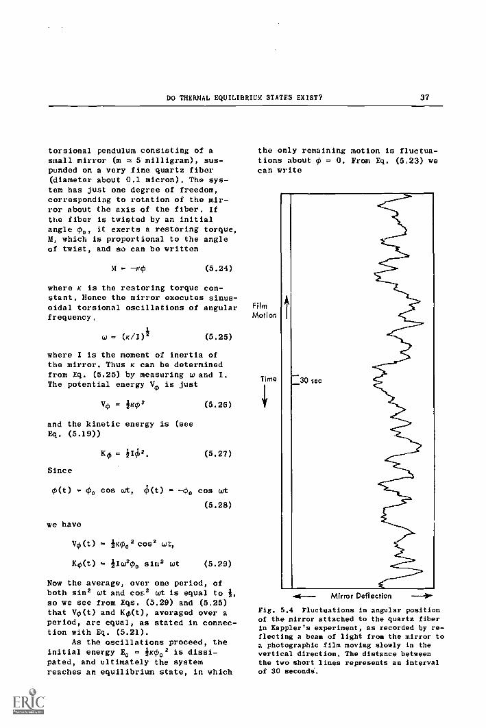
DO THERMAL EQUILIBRIUM STATES EXIST? 37

torsional pendulum consisting of asmall mirror (m 5 milligram), sus-pended on a very fine quartz fiber(diameter about 0.1 micron). The sys-tem has just one degree of freedom,corresponding to rotation of the mir-ror about the axis of the fiber. Ifthe fiber is twisted by an initialangle 00, it exerts a restoring torque,M, which is proportional to the angleof twist, and so can be written

M = -K0 (5.24)

the only remaining motion is fluctua-tions about 0 - 0. From Eq. (5.23) wecan write

where K is the restoring torque con-stant. Hence the mirror executes sinus-oidal torsional oscillations of angular Film

frequency. Motion

w = (x/01 (5.25)

where I is the moment of inertia ofthe mirror. Thus K can be determinedfrom Eq. (5.25) by measuring wand I.The potential energy V, is just

Vo = im02 (5.26)

and the kinetic energy is (seeEq. (5.19))

Ko = (5.27)

Since

0(t) = 00 cos wt, c(t) = -00 cos wt

(5.28)

we have

Vo(t) ix002cos2 wt,

K,(t) = 0000 sin2 wt (5.29)

Now the average, over one period, ofboth sin2 wt and cost wt is equal toso we see from Eqs. (5.29) and (5.25)that Vo(t) and K4(t), averaged over aperiod, are equal, as stated in connec-tion with Eq. (5.21).

As the oscillations proceed, theinitial energy E0 = ix002 is dissi-pated, and ultimately the systemreaches an equilibrium state, in which

Time

4

30 sec

Mirror Deflection

Fig. 5.4 Fluctuations in angular positionof the mirror attached to the quartz fiberin Kappler's experiment, as recorded by re-flecting a beam of light from the mirror toa photographic film moving slowly in thevertical direction. The distance betweenthe two short lines represents an intervalof 30 secondS.

38 HEAT AND MOTION

(Eu) = 2(iK) (02) = ksTs, (5.30)

where ks is the proportionality con-stant we have been seeking, between theaverage energy in mechanical fluctua-tions, and Tg (note that this constantis just twice the constant CI, whichwas introduced in the discussion ofEq. (5.22)). The constant ks is calledBoltzmann's constant, after the physi-cist who postulated the relation inEq. (5.17). Its value can be deter-mined from Eq. (5.30), once K has beenfound from Eq. (5.25), by measuring(02), the fluctuations in the positionof the mirror as it makes random oscil-lations about the fiber axis, in equi-librium. Kappler recorded the positionof the mirror by reflecting a pointlight source from it onto a photo-graphic film, which was moved slowlyin the vertical direction. An exampleof one of these records, showing fluc-tuations over a period of about halfan hour, :Is shown in Fig. 5.4.

Since (En) has the dimensions ofenergy, the dimensions of ks are en-ergy/degree, so its value depends onthe size of the degree for the temper-ature scale used. With the degree ap-propriate to the Tg scale, which wedenoted oslo, the best current valueis"

10This degree is the same as that on the commonmetric Celsius scale (CC), since the two scalesdiffer only by the displacement of their origin,

k s . 1.38054 x 10-16 ,:rg/°K or

ks = 1.38054 X 10-23 J/ °K,

where J is the Joule, the unit of en-ergy on the MKS scale, (1 J = 107 erg).

The small value of ks in cgs orMKS units explains why mechanical fluc-tuations are not commonly observed, butrequire special circumstances, such assuspensions of small particles, in or-der to be seen. From Eq. (5.30) we cansee that

(vu2(t)) (ks/m)Ts, (5.31)

so that for a mass as small as a micro-gram (say a cube of ice about 0.1 mm.

on a side), and a temperature in theneighborhood of room temperature (about3 X 102 °K), (v,2(t)) Al 4 x 10-3 cm2/sect. The observed speeds will be ofthe order of a(v,), or the square rootof (vu2(0), or m 2 x 10-4 cm/sec =2 micron/sec, and thus would be imper-ceptible without magnification. For amass of a gram, a(vu) will be 103 timessmaller yet.

that is, Tir(°N) Tc(°C) + To (see Eq. (4.4))where T, - 273.16 °K."Boltzmann's constant can be determined in avariety of different ways besides fluctuationmeasurements; in fact, fluctuations do not gibethe most precise value.

6 INTERNAL

6.1 REGULARITY IN RANDOM EVENTS.

DEGREES t REEDOM

The proportionality of Eq. (5.18),which, in view of Eqs. (5.21) and(5.30) can be written

(Ku) - 3k8Tg, (6.1)

expresses a remarkable regularity. Forit asserts that this average is a con-stant, in equilibrium, which has thesame value for every degree of free-dom, rotational as well as transla-tional. By virtue.of Eq. (5.21) theaverage of every potential energy con-tribution in an oscillating systemalso has the same value. But of course,Ku(t) fluctuates randomly as the ve-locity fluctuates, so Eq. (6.1) meansthat we have found order in the midstof chaos. It was pointed out at theend of the last section that (Ku) is avery small energy on a macroscopicscale of energies, but regardless ofits size, its very existence poses aproblem which we now investigate.

Actually, this sort of regularityin averages associated with randomevents is commonly observed, providedthat the number of random events islarge enough. For instance, if a faircoin is tossed N times, the order inwhich heads and tails appear is ran-dom. However, as N increases, the ratioof toils to heads, t/h, approachesunity. But in the sane limit, that is,ever-increasing N, the average of themagnitude of the difference between thenumber of headm and the number of tails,

tl) (WI), does not decrease.In fact, this average increases withoutlimit as N increases. Hence the se-quence of tails and heads remains ran-dom, no matter how long the game isplayed.

At first might, it might appearthat the statement, "Average of IAN) in-

creases, as N increases" is inconsistentwith the statement, "The ratio of tails

39

to hea4' 1 approaches unity as N in-creasc we can see that the twostatements ale compatible, in the fol-lowing way.

The average value of the ratio oftails to heads is

(t/h) ((h T IAN) /h) - 1 ; (IANI/h)

(6.2)

(Since IAN! is always positive, thepositive sign must be used in Eq. (6.2)if AN itself is negative.) As N in-creases, h, the number of heads, ap-proaches N/2, so Eq. (6.2) can be writ-ten:

(t/h)ft 1 T 2 (IAN!)/N (6.3)

Now as stated above, the average ofWI increases with N, but it does notincrease as fast as N. For large N,(IAN) is proportional to the square-root of N, that is, to Ni, so that as Nincreases, (t/h) approaches

(t/h) :*. 1 2/N3, (6.4)

and therefore the ratio (t/h) has thelimit unity, as N increases withoutlimit.

This discussion suggests that theconstant averages (vul(t)) and (Ku(t))must arise as limits like that inEq. (6.4). That is, they represent av-erages of some sort of repeated randomprocess, the number of whose repeti-tions is very large. Me must now ask,what is the nature of the random proc-ess involied? That is, what is thephysical origin of the observed result,that successive values of v1(t) differfrom each other?

If we are to retain the validityof Newton's Second Law, we must answerthat Ave vu(t2) vu(ti) can onlyarise from the action of a componentof force, Fu, acting during the time

40 HEAT AND MOTION

interval At = t2 ti. We have, fromN-II,

Av u = ft

Fu (t)(t) dt = 1 Ju (6.5)1

where Ju is the impulse. Now the sys-tems we have been describing, namelyparticles in a fluid suspension, aremechanically isolated from everythingbut the fluid itself. The suspendingfluid is therefore the only possiblesource of the required impulse Ju. Andthe origin of this impulse must besought in degrees of freedom associatedwith the internal structure of thefluid. We have so far neglected tomention these internal degrees of free-dom, for reasons which are discussedin Appendix 5.

Much of twentieth-century physicshas been devoted to an investigation ofthe internal structure of matter. Themodern atomic theory, based on quantummechanics, which has resulted from thiseffort, gives us a largely satisfactorypicture of this internal structure. Inquantum mechanics, the distinction be-tween the macroscopic and atomic lev-els is a fundamental one. It is basicto quantum mechanics that the degreesof freedom associated with the internalstructure of matter, which we shallhenceforth refer to as "internal de-grees of freedom," do not, in general,behave like small copies of those weare familiar with on the macroscopiclevel. For instance, we can never ex-pect to see an electron, no matter howrefined our techniques become, in thesame way that we can see pollen grainswhich are invisible to the naked eye,by using a powerful microscope.

Nevertheless, there are some re-spects in which the internal degreesof freedom do behave much like thoseof "classical" Newtonian particles, Asa result of this similarity, many re-lations between thermal and mechanicalproperties can be understood withoutinvoking quantum mechanics. The restof this monograph will be devoted toexamining some of these relations onthe basis of the behavior of the inter-nal degree& of freedom.

In the first place, from the dis-cussion of Eq. (6.5), we see that ifthe averages (Ku(t)) and (vu2(0) fora particle in a suspension are con-stant because the impulses Ju arisefrom random interactions with the in-ternal degrees of freedom, then thenumber of those degrees of freedom,(Ndj)/, must be large. From the defi-nition of Ndf in the last section, wewould expect (ial)/ to be of the orderof the number of atomic particles mak-ing up the internal structure of thesuspension. If there are Na of theseatomic particles (atoms or molecules),in the suspension and they are allmoving freely in three dimensions, then

(Nu1)1 3Na. (6.6)

Secondly, we now have a very sim-ple way of understanding the dissipa-tion of mechanical energy. Suppose wedrop a pollen grain of mass m, whichhas the temperature Tg' into a liquidat the same temperature. We give thegrain an initial downward speed vo. Itwill decelerate and quickly reach ter-minal velocity V?, which, as we haveseen, is very small. The initial me-chanical energy (m/2)vo2 has all beendissipated. Now at the outset, thismechanical energy was associated withjust one degree of freedom, namelythat of the center of mass of the pol-len grain, in the downward direction.The dissipation proceis consists sim-ply of the sharing of this energyamong all the internal degrees of free-dom, numbering (N0)1, of both the pol-len grain and the suspension. Beforethe pollen grain was fired into thesuspension, each of the internal de-grees of freedom had (Ku) ikTs' (see

Eq. (0,1)). Since the atomic particlesin the pollen grain are not movingfreely, but also possess potential en-ergy due to the elastic forces thatbind them to each other, the total en-ergy of each of their degrees of free-dom is given by Eq. (5.2l). Therefore,at the outset, the total mechanicalenergy of the system is

INTERNAL DEGREES OF FREEDOM 41

E t = imvo 2 + {2[ (NdOi izi.ain

+ (NO )1 suspension } (ikTg (6 .7 )

and from Eq. (6.6), we have

Et = 4mvo2 + {(3lags)16(Na)Kiain

+ 3 (Na) suspension(6.8)

If the total mechanical energy is con-served, then after the pollen grainhas come essentially to rest (sincevT sr 0) ,

Et (ikTg")[6(NOgrain

+ 3(N ) Terisitm )4 (6.9)

The final equilibrium temperature Tg"> Tg', since we know that dissipationincreases the temperature. The quan-tity in brackets in Das. (6.7) and(6,8) is called the internal energy,since it is associated with the inter-nal degrees of freedom, in contrast tothe term 3mv02, which is a property ofthe center of mass of the pollen grain.We will denote the internal energy byU, and we see from Eqs. (6. ?) and (6.8)

that it is a function of temperature.We can combine these two equations inthe form:

U(Tg") U(Tgl) AU 3mv02, (6.10)

or, in words, dissipation of mechani-cal energy increases the internal en-ergy.

We will discuss the internal en-ergy U further in the next section.Before doing so, we consider one fur-ther question connected with our dis-cussion of dissipation. According toour description of dissipation, energywhich is initially concentrated in onedegree of freedom, namely the amountimvol initially possessed by the z com-pon-nt of the motion of the pollengrain, is shared, during the approachto equilibrium, by all the degrees offreedom. Equilibrium is reached whenthis sharing is complete. We now in-quire as to the mechanism by which

this sharing takes place. In otherwords, how is macroscopic mechanical

converted toenergy, (Kz) tenter of mass,internal energy U?

The answer to this question doesnot require the introduction of anynew assumptions, at least for theBrownian motion of particles in a sus-pension, or for the molecules or atomsin a gasEach particle in the internalstructure possesses, on the average,an amount of energy equal to (K,) foreach degree of freedom. Hence each ofthese particles is incessantly moving,and therefore colliding with its neigh-bors. These collisions produce the im-pulses Ju. Since the collisions arerandom, their result is the uniformsharing of energy, on the average, byeach degree of freedom. In fact, wecan write an equation analogous toEq. (6.3), replacing t/h by the ratioof K for any two degrees of freedom,say Ki and K. Then, as in Eq. (6.4)

we have

(KI/Kj) a 1 (2/N3) (6.I1)

where now N is the (enormous, numberof successive collisions.

The same argument can be extendedto the internal structure of a solid.In this case, since the atoms or mole-cules are bound by elastic forces, theaverage energy is (E,) 2(Ku) per de-gree of freedom. Again, the continualmotion results in interactions whichprovide the impulses J,,. Once more,the result of the random impulses isthat each degree of freedom has anequal share of the total internal en-ergy.

Since we have been treating alldegrees of freedom, those associatedwith the macroscopic model as well asthose of the internal structure, on anequal footing, it should be possibleto construct a macroscopic models' ofthis equalizing process, which we will

iiNotice that here, the word model is taken inthe literal sense, like that of the ball and rodmodel cf the solar system referred to in foot-note I.

42 HEAT AND MOTION

refer to as "equipartition of energy."The game of billiards is an example ofa model for the internal structure ofa gas. Initially only the cue ballpossesses K, but after it hits theother balls, which were initially atrest, they all share in the motion.The process is somewhat obscured byfriction between the balls and thetable. A better model can be con-structed by placing smooth disks on asmooth table with many small holesthrough which air is forced, so thatthe disks are supported on a cushionof air. A photograph of such a modelis shown in Fig. 6.1. Friction is verymuch smaller on such an air table thanon a pool table, so that the approach

Fig. 8.1 General arrangement for observingtwo-dimensional collisions with negligiblefriction. The camera at the top of the tri-pod is focused on the air table on thefloor. A wire strung along the edge of theair table serves as a rough approximationto a (nonuniform) temperature bath when themotor in the foreground rocks the tableabout a vertical axis. The pump which forcesair through the hcle In the table can beseen in the right background.

to equilibrium can be followed for amuch longer time. It is fount that theratio in Eq. (6.11), which here can bemeasured directly by using strobo-scopic illumination to measure vu(t),as shown in Fig. 6.2, rapidly ap-proaches unity. Further, by usingdisks of different mass, as shown inFig. 6.3, the proportionality statedin Eq. (5.16) is also confirmed.

To the degree that the behaviorof the macroscopic degrees of freedomassociated with the motion of the cen-ter of mass of the disks (for each

10-

0

Fig. 6.2 A multiple exposure with strobo-scopic illumination, using identical disksin the arrangement of Fig. 6.1. A collisiontook place hear the bottom of the figure.

INTERNAL DEGREES OF FREEDOM 43

disk, Ndf = 2 if rotation is neglected,Ndf = 3 if rotation is considered), issimilar to that of the internal de-grees of freedom, this model providesa convenient way of examining the ap-proach to equilibrium in detail.

6.2 INTERNAL ENERGY

Our definition of internal energyof a system as the total mechanicalenergy associated with all the degreesof freedom of its internal stt.Jo.ture

(which we have called "internal de-grees of freedom") was deceptivelysimple." We approached the definitionthrough the examination of fluctua-tions in free macroscopic particles,although we have also referred to os-cillating systems in passing. For afree macroscopic particle, we have as-serted that (Ku) is related to Tg byEq. (6.1) and for a macroscopic oscil-lator, Eq. (5.21) relates (E,) to Tg.We will refer to these as "classical"relations, since they are obeyed bymacroscopic degrees of freedom, and wewill call any degree of freedom, mac-roscopic or internal, for which thesehold, a "classical" degree of freedom.Now both of these results are examplesof the "lamppost" tectnique describedIn section 1. We have stressed in var-ious places, and especially in Appen-dix 5, that in general, internal andmacroscopic degrees of freedom cannotbe expected to behave alike. That is,it is most unlikely that internal de-grees of freedom will behave "clas-sically." Hence we may wonder howEqs. (6.1) and (5.21) can be used indiscussing internal energy, or even ifthey can be used for that purpose at

-..1113$11otice that ve exclude from the internal en-ergy any mechanical energy that an Internal de-gree of freedom, in a rigid body, possesses byvirtue of the motion of the center of mass ofthe body. That Is, the motion corresponding tointernal energy is motion relative to the centerof mass. It is therefore described In a coordi-nate system in vhich the center of mass of therigid body Is at rest.

A01.14,nria. ill

.0*

Fig. 8.3 The same as Fig. 8.2 with largeand small disks.

all. There is just one physical systemthat is a reasonable approximation toa collection of free particles on theatomic level - a gas at low pressure.The suspension of fine particles wehave been discussing is also a reason-able approximation, but on a macro-scopic level. And our analysis showed(see Eq. (5.13)), that in this systemthe relation between measurable speedsand Ts contains the constant N, whosevalue cannot be determined. In sec-tion 5.3, we discussed a macroscopicsystem whose fluctuations do give avalue for ka. But as stressed in Appen-dix 5, the assumption that all internal

44 HEAT AND MOTION

degrees of freedom behave like macro-scopic ones, is in general unwarranted.

In the next section, we shall seehow departures from classical behaviorby the internal degrees of freedom canbe observed in purely macroscopic meas-urements. The rest of this section isdevoted to two other matters. First,we make more explicit how to distin-guish between mechanical energy, whichis our name for energy associated withdegrees of freedom associated with themotion of the center of mass or of ro-tation about the center of mass (weshall refer to these as "center of massdegrees of freedom"), and internal en-ergy, belonging to the degrees of free-dom of the internal structure. Then wediscuss how the internal energy can berelated to the macroscopic equilibriumproperties, the (Pi), which we intro-duced in section 4.1.

6.2.1 Mechanical Energy and InternalEnergy

The first problem, of distinguish-ing between mechanical energy and in-ternal energy, is important because webased our introduction of internal de-grees of freedom in the last sectionon complete equivalence, so far assharing energy is concerned, betweenthe degrees of freedom of the centerof mass and those of the internalstructure. If there were no qualifica-tions to this equivalence, then theparticle model could not possibly de-scribe motion adequately, even formacroscopic objects. For the particlemodel ignores the internal degrees offreedom completely. In fact, a usefuldefinition of a "mechanical system"(in contrast to a "thermal system"),is one in which only changes in me-chanical energy due to external forcesneed be considered. In such an ideal-ised system, the internal energy isconstant, unaffected by the motion ofthe object or by the forces acting onit. Hence, mechanical energy is con-served, and there is no sharing of en-ergy with the internal degrees of free-dom (no dissipation). We must therefore

inquire how it can be that conversionof mechanical energy into internal en-ergy occurs in all real systems, whilethe ideal mechanical system is actuallya useful abstraction, despite the factthat it ignores all internal structure.

Of course, every macroscopic ob-ject has internal structure, and in-ternal degrees of freedom associatedwith it. This structure is very com-plex; it comprives molecules, whoseconstituent atoms themselves are madeof electrons and nuclei, which in turncoasist of neutrons and protons. Itturns out, as we shall see in the nextsection, that equipartition of energydoes not apply to all the internal de-grees of freedom. However, at leastsome of them behave "classically," asdefined earlier in this section, andthe following remarks apply only tothese.

Let us examine the consequences,for these classical internal degreesof freedom to which equipartition ofenergy does apply, of giving a veloc-ity, V, to the center of mass of anobject which was initially at rest.The mechanical energy, of course, isincreased by 3mV2. When the object wasat rest, the components of the inter-nal structure were subject to interac-tion forces which we denote (Fu)0 (seeEq. (6.5)). These forces are responsi-ble, as we have seen, for the attain-ment of equipartition of energy amongthe classical degrees of freedom. Whenthe center of mass is moving with ve-locity V, we denote the interactionforces (Fu)y. We now ask, what is therelation between (Fu)o and (F00

We recalled above that the parti-cle model is an ideal abstraction inwhich dissipation does not occur, andthat dissipation is simply the conver-sion of mechanical energy into internalenergy. Now when our object is at rest,we know that the interaction forces(Pp)0 do not change the mechanical en-ergy. An external force is required toset the object In motion. In referringto an ideal situation in which dissi-pation does not occur, the particlemodel embodies the assumption that the

INTERNAL DEGREES OF FREEDOM 45

interaction forces (Fu)y, which actwhen the object is moving with veloc-ity V, do not change the mechanicalenergy, 3mV2, either. Now if this werenot a good assumption, the particlemodel would not be a useful abstrac-tion at all. In fact, no reasonablemodel could be made, which, like theparticle mcdel, ignores the internalstructure.

This assumption about the inter-action forces (Fu)v could, of course,be justified by the success of the par-ticle model. But the remarkable fea-ture about this property of the inter-action forces is that it does not re-quire a special assumption at all. For,as we discussed at the beginning ofsection 4, forces are the same in allreference frames moving with respectto each other with constant velocity."(Such frames are all "inertial frames"with respect to each other.) Therefore,when we give a macroscopic object aconstant velocity V, we do not changethe internal interaction forces at all.Hence, the forces (Fu)y, like theforces (Fu)0, do not affect the mechan-ical energy, because (Pu), (Fu)0. Asa consequence, the energy associatedwith the macroscopic motion is notshared with the internal degrees offreedom, unless there is some kind ofnew force exerted on the body as a re-suit of the motion. Such forces areprovided by friction, when the objectmoves in a resistive medium, or by theimpulses occurring when it strikes anobstacle. These forces will then pro-duce dissipation, and ultimately resultin the sharing of the macroscopic en-ergy among all the internal degrees of

Mlles an object is rotating about its center ofsass, the reference frame is which it is at restis not an inertial frame with respect to thereference frame in which the object is rotating.Hence the internal forces are affected by rota-tion, and the argument given hue does not hold.Thus, is order for the particle node) to bevalid for rotation, the special assusiption Isrequired, that the changes in interaction forcesdue to rotation do sot, by themselves, lead toappreciable dissipation.

freedom, thus increasing the internalenergy.

6.2.2 Macroscopic Properties andInternal Energy

We now turn to the relation be-tween internal energy and the macro-scopic properties, (P1), of an objectin thermal equilibrium. The expressiongiven in Eq. (6.10) for the increasein internal energy resulting from thedissipation of mechanical energy, is alittle misleading. In that equation, Uwas written as a function of tempera-ture only. This is certainly true forthe classical degrees of freedom of afree particle. But in general, if wewish to express the internal energy ofa.system whose internal degrees offreedom are more complicated, we muqtexpect that U will depend on otherproperties of a thermal equilibriumstate besides Tg. Thus we may write

U U(Tg,Pj).

If we do this, we might appear tobe back at the point at which we wereled to introduce the concept of tem-perature. The internal energy has aunique value in each thermal equilib-rium state (we will describe this prop-erty of the internal energy by callingit a "function of state"), but unfor-tunately, other properties besides thetemperature, and conceivably manyother properties, might be required inorder to specify the state and hencethe internal energy. But again, thefact that the number of internal ae-green of freedom is enormous comes toour rescue, as it did in establishingEq. (6.1).

All of the properties Pi of a mac-roscopic thermal system in equilibriumare related to averages of correspond-ing properties of components of the in-ternal structure. For instance, thevolume Vs, is the product of the num-ber Na of atoms or molecules, and theaverage volume (Vs) associated witheach of the atoms or molecules. Be-cause of the fluctuations in the posi-

46 HE AT AND MOTION

tions of the individual atoms of mole-cules, Va will vary from one to thenext, but because of the enormous num-ber of atoms or molecules, (V,) willnot, in general, have detectable fluc-tuations, so there will be no observ-able fluctuations in V8 either. Thesame sort of argument holds for otherproperties Pl.

Now we have seen that for con-densed matter the elements of internalstructure are not free. The interac-tion forces among them will in generaldepend on distance, since they arebasically of electrical origin. Hencethe potential energy of the internaldegrees of freedom will depend on Va,and therefore the average potentialenergy (Vu) will be a function of(Vs). Therefore, we may expect in gen-eral that the internal energy, U, in athermal equilibrium state is a func-tion of Vs, the volume of the system,as well as a function of Tg: UU(Tg,V.). All the other Pi will alsodepend on either Ts (through (Ku)), oron Vs, so we would expect that justthe two macroscopic variables, Tg andVs, would completely determine all theP1 in a thermal equilibrium state.

This expectation is borne out,provided that (Yu) depends only on theaverage separation of the atoms ormolecules, as expressed by (VA). Ifthe atoms have a net magnetic moment,however, then (Va) will also depend onthe external magnetic field H or themagnetic induction B, and U U(Ti,Vs,H).

Or if dipole moments are also present,U will depend on the electric field, E,so U U(Tii,Vs,H,E) in this case. Fi-nally, the eJpendence of (Vu) on (VA)may be different in different chemicalspecies, so if a system is chemicallyheterogeneous, that is, if it containschemical species Mt, Ms then

U will depend on the relative amountsOf each, mi(111), NA(MA) . . , UU(TI,VA,m1,111 . . .), if no magneticmoments or electric dipoles are pres-ent.

We can conclude from this discus-sion that since the internal energyis a function of the thermal equilib-

rium state in the sense defined, thethermal equilibrium states must beuniquely defined by just the limitednumber of macroscopic variables thatappear in the ..arious parentheses asarguments of the function U. Hence re-lations among different thermal equi-librium states can be expressed purelyin terms of macroscopic variables,with no need at all to mention the var-iables on the atomic level to whichthese macroscopic variables are re-lated. The remark "no need at all" re-quires some qualification, however.There is a need to inquire about theinternal structure, if we are inter-ested in the source of the order thatis observed on the macroscopic level.Nevertheless, it remains true that forcrtain purposes such inquiry aboutthe atomic level is a luxury. Thestudy of relations among thermal equi-librium states, which is the subjectof "classical thermodyramics," is avery powerful tool for investigating alarge class of natural phenomena. Muchof the study of chemical reactions,for instance, can be treated entirelyby classical thermAynamics.

6.3 HEAT AND HEAT CAPACITY

We see from the above discussionthat 4.1', as a result of some operationperformed on a system In a thermalequilibrium state, which we will de-note Si, the internal energy U of he

system is changed, then the systemmust have undergone a transition to anew state, say S,. Now the applicationof a force to an object which is freeto move is not such an operation; thecenter of mass will acquire kineticenergy equal to

(6.12)

where rile its initial position vec-tor, rs is the position vector atwhich the force is removed, and p(;)is the net external force applied sothat the integral in Eq. (6.12) is the

INTERNAL DEGREES OF FREEDOM 47

work done on the object. As we haveseen, the internal energy of a systemhas a value which is independent ofthe mechanical energy of its center ofmass, although as a result of naturallyoccurring process this mechanical en-ergy is sooner or later dissipated intointernal energy.

It is possible, however, for aforce to do work which changes the in-ternal energy of a system. For in-stance, if the force is applied to arigid body which is constrained sothat it can't move, the work done bythe force is stored as elastic inter-nal energy in the rigid body .15 Theelastic energy is internal energy be-cause, in this case, the force deformsthe body. So Vs is changed, and there-fore so is (Va); and we have seen thatc/u), and therefore U, depends on (1/1).(Does this argument hold for shear de-formation, in which only the shape,but not the size, of the object ischanged?) In both of these cases, thatis, a rigid body (a) whose center ofmass has been given kinetic energy (be-fore this has been dissipated into in-ternal energy and the body has some torest), or (b) which has been givenelastic potential energy, the workwhich has been done can all be recov-ered as mechanical energy. For in-stance, the object with kinetic energy,K, can be brought to rest by having itlift a weight, so that K is convertedinto gravitational potential energy,

In general, however, work whichhas been converted into internal energy

"This description is, to some extent, a contra-diction In terms. The 'l'al rigid body, Intro-duced as an abctraction In classical mechanics,has a fixed voluee Vi, ehIch Is independent ofexternal forces, la order to discuss elasticforces, as we have just done, a different model,the "elastic holy" is introduced. However, thetheory of elasticity, which has been extensivelydeveloped, starting early in the nineteenth cen-tury, treats the elastic body as a mathematicalcontinuum, without any discrete internal stn.:-ture. It regards such a body as made up of geo-metrical points, much in the sane way as we re-gard space, and does not introduce the notionsof atoms or molecules.

cannot be completely recovered. A com-plete discussion of the conversion ofinternal energy into work is well be-yond the scope of this monograph, sowe will conclude with a further discus-sion of the reverse process, the per-formance of work on a system so as tochange its internal energy. We will beinterested in two of its aspects inparticular: first, to describe in moredetail how it is related to measure-ments of internal energy; and second,to show briefly how some very importantproperties of the internal degrees offreedom can be deduced from measure-ments of internal energy.

We have already given brief atten-tion to the first question, measure-ment of internal energy, when we wroteEq. (6.10). We will rewrite the rela-tion stated there as

U(Sf) - U(Si) - AU - AWA. (6.13)

In this lelation, Si and Si refer tothe initial and final states respec-tively, as identified by their respec-tive values of Ts, Vs, and whattverotte=r macroscopic variables are neededto specify them completely (for in-stance, electric field, E; magneticfield, H, etc.)." The subscript A isattached to the expression for thework done, to emphasize that this re-lation holds only under special circum-stances, namely, when work is performedon the system, with the system ther-mally isolated from its surroundings.Such a process is called an "adiabaticprocess," and the subscript A was cho-sen to refer to the tern adiabatic.

The reason for attaching this con-dition of thermal isolation, that is,requiring that the process be adia-batic, is that the internal energy canalso be changed without any work beingdone on the system. We have stressedthe fact that the temperature of a sys-tem will change if it is placed inthermal contact with another system at

"Note that it the system does mechanical workat the expense of its internal energy, AV willbe negative, and so will Ala.

48 HEAT AND MOTION

a different temperature. Since U is afunction of Tg(as well as other varia-bles), a temperature change correspondsto a change in U (as indicated inEq. (6.10)), provided that the othervariables which define the state 8,remain constant. In what follows, weshall, for simplicity, consider onlysystems for which U = U(Tg,Vs) and noother variables. For such a system,then, if its volume, Vs, remains es-sentially constant, a change in TR im-plies a change in U. Hence we have as-serted that changes in U occur in sys-tems with constant Vs, when they areplaced in thermal contact with a sys-tem at a different temperature.

This process, exchange of inter-nal energy between systems originallyin thermal equilibrium at differenttemperatures after they are placed inthermal contact, is usually referredto as "heat transfer." The term "heat"means simply internal energy which isexchanged between systems in thermal con-tact, in the course of their approachto mutual thermal equilibrium. If thisexchange is not accompanied by the per-formance of any work, that is, if it isa purely thermal process, Then there isno other change in U.

Suppose we have a system labeled"1," initially in thermal equilibriumstate at at temperature T,1 (henceforth

the subscript g on T will not be wr t-ten, although it is still implied thatwe are using the gas-thermometer scale)placed in thermal contact with asystem labeled "2," initially inthermal equilibrium in state SRI attemperature Tit. When placed in ther-mal contact, they reach states Sif and82t, which have the same temperature,Tf. If the two systems are in thermalisolation from all surroundings buteach other, and if no work has beendone on either system, then

U(s11) + mit) u(sit) +

(8,14)

since there has been to change in thetotal internal energy of the two sys-

tems taken together. If we transposeterms, we have

u(s,f) U(S11 [ U(S21) u(s21 )]

(6.15)

or AU, = AU2. (6.16)

Each of the terms in Eq. (6.16) repre-sents an internal energy change due toheat transfer. Such internal energychanges are usually denoted in a spe-cial way, by the letter Q:

AU1 a 6%; AU2 AQ, (6.17)

and we see from Eq. (6.16) that

AQ2 4A1 (6.18)

In common parlance, AQ is often re-ferred to as "an amount of heat," butwe see from our discussion that suchan expression can be misleading. Theword "amGalt" is usually associatedwith a substance that can be obtainedin isolation; we speak of "an amountof money," for example. But "heat" isnot a substance in this sense at all.It merely represents a change in in-ternal energy, U, occurring in a cer-tain specified way, namely, as the re-sult of thermal contact alone.

If we consider a general process,in which U changes both by thermal con-tact and by the performance of mechan-ical work as well, we can combineLots. (6.17) and (6.13), and write

AU AW 4 /IQ. (8.19)

(Note that we have omitted the sub-script A on AW, since now the processis no longer adiabatic.) This relationis called the First Law of Thermodynam-ics. We see that it expresses the con-servation of internal energy, and thusis a generalization of the conservationof mechanical energy of macroscopic de-grees of freedom. The actual historicaldevelopment which led to its assertionwas very different from the way inwhich we arrived at its statement.

INTERNAL DEGREES OF FREEDOM 49

That development took place before anybut the vaguest notions had been estab-lished, concerning internal degrees offreedom. As a result, Eq. (6.19) wasfirst stated as a generalization frompurely macroscopic measurements, espec-ially those of Joule. He performed me-chanical work on various fluid systems,such as baths of water and mercury.The center of mass of the liquid alwaysremained at rest, so none of the workAMA became macroscopic kinetic energy;it was all dissipated into internalenergy. The fluids were in thermal iso-lation from their surroundings. Jouledetected the change in internal energy,AU, by measuring the resulting changein temperature, AT. He found that fora given fluid system, exactly the sameAT was observed for a given expendi-ture of work AMA regardless of the man-ner in which the work was dissipated;he used frictional processes of differ-ent sorts, and electrical dissipationas well. (The heating of a wire throughwhich an electrical current passes isnow called "Joule heating.") He argued,as we have done, that since Ti and Tfwere the same in each case, that thedifferent processes he used alwaystook the system from the same initialthermal equilibrium state to the samefinal equilibrium state (changes involume V4 were negligible). Hence hewas able to conclude that AU was thesame in each case. Since the value ofAU did not depend on the particularprocess he employed, that is, on themanner in which AMA was dissipated,or on the particular fluid system inwhich AMA was dissipated, he concluded,as we did earlier, that U, the inter-nal energy, is a "state-function" inthe sense that we defined. Thus Joulewas able to assert the validity ofEq. (1.19) without making any assump-tions whatever concerning the Internalstructure of matter, or the internaldegrees of freedom associated with thatstructure. Not only was Joule's argu-ment a success, so were further deduc-tions concerning the connection be-tween macroscopic thermal and mechani-cal behavior that could be shown to

follow from it. Those successes actu-ally inhibited acceptance of a*omictheory to a certain extent toward theend of the nineteenth century, as dis-cussed in Appendix 5.

Equation (6.19) describes onlychanges in internal energy, and notany actual values of the internal en-ergy in a particular state, which wehave been denoting U(S2), U(S2), etc.So macroscopic measurements can onlyallow us to determine such differencesAU. Still, these differences, measuredmacroscopically, can give informationabout the internal degrees of freedom,whose behavior they represent.

First, let us describe how AU maybe determined in practice. For the sim-ple systems we are describing, inwhich the state S is determined by Tand Vs alone, if Vs is held constant,AW = 0, so from Eq. (6.19)

AU - AQ. (6.20)

Now AQ can be measured by dissipatingmechanical energy completely; a con-venient way of doing this is by pass-ing an electrical current though awire. If the electrical energy is dis-sipated at a constant rate, E, for atime At,

AQ At - AU. (6.21)

If the system remains homogeneous,that is, if it does not transform fromsolid to liquid, or liquid to vapor,this dissipation is accompanied by atemperature change AT. The ratio

A'4. AT C (6.22)

Is called the "heat capacity." Underthe conditions we have been describing,that is, tonstant volume so that AW 0,

the ratio in Eq. (6.22) is the heat ca-pacity at constant volume, denoted C,,and we see from Eq. (6.20) that

Cs - AU/AT. (6.23)

Therefore, measurements of heatcapacity at constant volume give di-

50 HEAT AND MOTION

rectly the way in which U changes withtemperature, and indirectly, corre-sponding information about (Es), theaverage mechanical energy per atom.

We shall discuss just one exampleof this sort of investigation. Althoughit deals with a very simple system, itstill displays the inadequacy of clas-sical mechanics as applied to internaldegrees of freedom.

The system we investigate is amass of gas. We have already remarkedthat all gases behave alike in conform-ing to Eq. (4.5) at sufficiently lowpressure. This behavior is simplest tounderstand on the atomic model, inwhich a gas is just a collection ofparticles which are independent exceptfor collisions. The collisions changeKu for the pair of colliding parti-cles, but as we saw at the end of sec-tion 5.2, they bring about thermalequilibri'lm, in which (Ku) is a con-stant, and the same for each degree offreedom. Now in dense gases, at highpressure, the particles are closeenough to exert mutual forces evenwhen they are not colliding, and thesewill also make a contribution to (EA).But when the pressure becomes verysmall, these forces, which depend onthe average distance between particles,

5

3

4

1

3,5

3

cv

also become very small, so (Es) (Ks).

Therefore

U = (Ndf)/(ikT) (6.24)

according to Eqs. (5.18) and (6.1).Hence from Eq. (6.23),

C, = (Ndt)1(1k). (6.25)

A system such as this, in which UU(T) only, that is, with no dependenceon Vs or any other variable such as Eor H, is called an "ideal thermal sys-tem." As we have seen from F4. (6.25),such a system has a heat capacitywhich is independent of T.

While no such ideal thermal sys-tem, such as the ideal gas we havebeen describing, exists in nature, agas at low pressure is a reasonablygood approximation. But strangely, inhydrogen, for which measurements of Crare shown in Fig. 8.4, the expectationof a constant value which is independ-ent of T, is not confirmed. Betweenabout 300°K and 80 °K, Cy decreases bythe ratio 5 to 3. Now hydrogen gas isknown from chemical evidence to formdiatomic molecules, Hy, in the gasphase. The observed decrease can onlybe interpreted by assuming that (Heidi

....... t 40 80 120 160 200 240 280 'K

Fig. 6.4 The heat capacity at constant volume of one sole of hydrogen gas, as a functionof temperature.

INTERNAL DEGREES OF FREEDOM 51

has decreased by the ratio 5/3 in thistemperature interval. The denominatorof the fraction, 3, is just the numberof degrees of freedom of a free parti-cle; the numerator, 5, suggests thatwhen the temperature reaches about300°K, the H2 molecules have somehowachieved two additional degrees offreedom. From other evidence, theseextra degrees of freedom represent ro-tation about two axes perpendicular tothe axis of the molecule itself. Atstill higher temperatures, Cv increasesfurther, in the ratio 7/5 to the valueat about 300°K. Thus, two further de-grees of freedom contribute to (Ea) athigh temperatures; these are probablyassociated with vibrations along theaxis between atoms in the molecule.Thus the classical model adequatelyexplains the constant portions of thecurve Cv(T); but it has no way at allof accounting for the observation that(NdOt is also apparently a functionof T. This result turns out to be aconsequence of a fundamental featureof quantum mechanics as applied to theinternal degrees of freedom. The ex-pression for (Eu), as calculated byquantum mechanics, is considerablymore complicated than the classicalone, Eq. (5.30), in which (Eu) is sim-ply proportional to T.

We cannot describe this quantum-mechanical result in detail, but aqualitative discussion can show how itleads to an apparent dependence of(licit)! on T. As we just saw, belowabout 80°K, the only degrees of free-dom of the H2 molecule whose energyvaries with T are those of the three-dimensional translational motion ofthe center of mass of the molecule.These degrees of freedom behave clas-sically; there is equipartition of en-ergy among them, each one's share beingiksT. All the other internal degrees offreedom of the molecule can be de-scribed as "frozen."I7 Their energy is

"At one time, the word "ankylosed" was proposedto describe such degrees of freedom, but fortu-nately, it never gained much currency.

not a function of T, so they do notcontribute to the heat capacity.

Now the possibility of a frozendegree of freedom, one whose energydoes not depend on T, can arise in theparticle model of classical mechanics,if the motion in that degree of free-dom is somehow constrained, For in-stance, as long as the disks describedat the end of section 5.3 must move ona horizontal plane surface, they haveonly two degrees of freedom; the third,corresponding to vertical motion,might be described as frozen. In thecase of the hydrogen molecule, theclearest indication of nonclassicalbehavior is the gradual "thawing" oftwo degrees of freedom, that is appar-ent in Fig. 6.4 between about 80°K andabout 300°K. As mentioned above, thereis evidence, which we cannot discusshere, that these two degrees of freedomcorrespond to rotation of the moleculeabout two axes, perpendicular to theline joining the two H atoms whichmake up the H2 molecule. Above about300°K, these two degrees of freedomare unfrozen, and behave classicall).

As a result of the quantum-mechan-ical phenomenon of "thawing" in the ro-tational degrees of freedom, Cv in-creases, between 80°K and 300°K, fromthe constant value corresponding tothree classical degrees of freedom, tothe constant value corresponding tofive classical degrees of freedom.Therefore, in a temperature regionwhere some of the degrees of freedomare classical, while all the rest arefrozen, Eq. (6.25) correctly accountsfor the heat capacity, provided thatthe factor (Ndf)! is interpreted asthe number of classical degrees offreedom.

The temperature region, in whicha degree of freedom makes its transi-tion from being frozen to behavingclassically, occurs at different tem-peratures for different degrees offreedom. We have seen that this tran-sition temperature region is between80° and 300°K for the two rotationaldegrees of freedom. Above 300°K, theheat capacity of H2 remains constant

52 HE AT AND MOT ION

until about 600°K, when another degreeof freedom begins to thaw, that corre-sponding to vibration of the two H at-oms which make up the molecule, join-ing them along the line. The heat ca-pacity then begins to increase again,but this degree of freedom does notreach its full classical contributionof Ice (why not iks?), until a tempera-ture of several thousand degrees isreached. By that temperature, the in-ternal structure of the H atoms them-selves begins to contribute to theheat capacity, as the atoms begin tobe ionized. They lose their electrons,and another aspect of the internalstructure of the H2 molecule becomesapparent. Thus, we see how successivethawing of different degrees of free-dom leads to a dependence of (Ndf)I,interpreted as the number of classicaldegrees of freedom, on T.

The freezing of degrees of free-dom at low temperature, and their thaw-ing as the temperature is raised, is aconsequence of the general propertywhich follows from quantum mechanics,that the energy associated with everydegre3 of freedom is "quantized." Thisquantum-mechanical property is best ap-preciated by contrasting it with thecorresponding situation in classicalmechanics, in which a degree of free-dom can have any energy whatever. Forinstance, according to Eq. (5.27), thekinetic energy associated with rotationis

Ko = = 31w2. (6.26)

Since the angular momentum, L, is

L = 1(44

we can write Eq. (6.26) as

Ko = L2/2I

(6.27)

(6.28)

In classical mechanics, there is norestriction on the angular momentum;L can have any value, and, correspond-ingly, the rotating system can haveany value of Ko. According to quantummechanics, however, the angular momen-

tum of a rotating system can take ononly certain discrete values. For a H2molecule at low temperature, with thevibrational motion frozen so that thedistance between the two H atoms isconstant, this restriction takes theform

L2 = 112 r(r + 1), (6.29)

where r is an even integer, r = 0,2,4,. . . and 11 in Planck's constant,

= 1.05 x 10-27 gm cm2/sec.

(Note that since the unit of energy,the erg, has dimensions gm cm2 /sect,the dimensions of 11 caa also be statedas erg sec.) Hence the only possiblevalues of Ko are those in the sequence

(Ko)r = Ch2/21) r(r + 1) erg. (6.30)

Thus, in the lowest possible energystate for rotation, the "ground state,"r = 0, and (K0)0 = 0, while in the firstexcited state for rotation, r = 2, and(1(0)2 = 602/21).

The quantum-mechanical character-istic, of frozen degrees of freedom atlow temperature which thaw as the tem-perature increases, arises because ofthe finite difference in energy be-tween the ground state and the firstexcited state, which occurs in allquantum-mechanical systems. As long asT is so low that the energy ksT isvery small compared to the differencein energy between the ground state andthe first excited state, which we de-note (AE)s, the degree of freedom re-mains frozen; when ksT begins to be ofthe order of magnitude of (AE)e, thedegree of freedom begins to thaw; andwhen keT has become about the samesize as (AE)e, thawing is complete,and the degree of freedom behaves clas-sically, and shares in equipartitionof energy. In the case of the H2 mole-cule, the moment of inertia can becalculated, since the mass of each Hatom is ms = 1.67 x 10-24 gm, andtheir separation, R, is R = 0.74X 10-8 cm, so I = 0.46 x 10-4° gm cm2.

INTERNAL DEGREES OF FREEDOM 53

Hence, from Eq. (6.30), (AE)0 is about8 x 10-14 erg. We have seen fromFig. 6.4 that thawing of the rota-tional degrees of freedom is essen-tially complete when T = 300°K, whichcorresponds to kBT about 4 X 10-14 erg,

or about one-half (AE)e.The same sort of situation exists

with respect to the vibrational motionof the H atoms with respect to 'machother, along the line joining them.For such vibration, the allowed valuesof the energy are, according to quan-tum mechanics,

(Eu)n = hw (n + i) (6.31)

where n is an integer, n = 0,1,2, . . .

and w is the angular frequency of vi-bration, determined by the mass of theH atoms and the restoring force con-stant (see Eq. (5.25) for an analogousexpression applying to torsional oscil-lation). Hence in this case, (62), isjust (AE)e = 1144.). The angular frequencyfor vibration of the H2 molecule isabout 8 X 1014 rad/sec, so (AE)e isabout 80 X 10-14 erg, or about tentimes larger than that for the rota-tional degrees of freedom. Hence thethawing of the vibrational motion doesnot occur until the temperature isabout ten times as large as that re-quired for thawing the rotational mo-tion, as described above.

Apart from this quantitative dif-ference, the rotational and vibra-tional degrees of freedom also differin an interesting qualitative respect.

We have seen that for rotational mo-tion, (K00 - 0, but in the vibrationalground state, according to Eq. (6.31),

(Eu)c, = flo # 0. Hence, while it istrue, that as T approaches zero, allinternal degrees of freedom tend tooccupy their ground states, it is nottrue, as is sometimes incorrectlystated, that "at T = 0, all molecularmotion ceases." As we have just seen,rotation does cease, but because(Eu)0 * 0 for vibration, vibration con-tinues, even at T = 0.

However, in all cases, the energyin the ground state is not a functionof T, so an internal degree of freedomin its ground state makes no contribu-tion to the heat capacity. Hence, whenthe ground states of the internal de-grees of freedom become occupied asthe temperature approaches zero, Cyapproaches zero for all macroscopicsystems. This property of Cy is closelyrelated to the third law of thermody-namics, which is discussed briefly inAppendix 3.

That our discussion is concludedat this point should by no means betaken to imply that all of the detailsof our subject have been exhausted. Al-most exactly the opposite is true; wehave barely scratched the surface. Butour goal, as stated at the outset, wasrather limited, and we have given atleast the beginnings of an answer tothe question posed there: How can ther-mal phenomena be incorporated, in a co-herent way, in the mechanical model ofmotion?

Appendix 1 TERMINAL

We choose a coordinate system as de-scribed in the text, with the positivez axis (and therefore the k unit vec-tor), pointing up. Since we are con-cerned only with motion along the zaxis, we need no subscripts; v willdenote the speed along this axis.

For a particle falling freely theacceleration is negative (downward),and has magnitude g, so (N-II) gives

m(dv/dt) = -mg, (A1.1)

where -mg is the gravitational forceon the particle. In a resistive medium,there is an additional force which wewill denote f, that retards the motionand is therefore directed opposite tov. This force does not depend on v ina simple way over a wide range ofspeeds. We shall therefore apply the"lamppost principle" discussed in thetext, and assume a simple form for thespeed-dependence of f, namely, f pro-portional to v. Because it is a retard-ing force we write

f = -kv, (A1.2)

where k is a constant of proportion-ality. (What are its dimensions?) Al-though this form for f is not gener-ally valid, it has the virtue that theresulting equation of motion is some-what easier to solve than a more real-istic version, f « v2.

Equations (A1.1) and (A1.2) thengive for a particle falling in a re-sistive medium,

dv/dt = -g - (k/m)v. (A1.3)

This equation is inhomogeneous, sinceit contains the constant term g, whilethe other two terms involve the varia-bles v and t. One particular solutioncan be found immediately, correspond-ing to equilibrium motion at constantterminal speed, v = -vT. In this casedv/dt - 0 so

54

SPEED

v = -mg/k; vT = mg/k. (A1.4)

From the intuitive discussion in thetext, this solution corresponds to thesituation after the particle has beenfalling a long time, that is, fort It is not correct when the par-ticle is just beginning to fall. Weneed, in addition, a solution which isvalid for finite t, and which reducesto the ideal value v = -gt for t v 0.Such a solution, combined with (A1.4),will describe the motion at all times.

A solution valid for finite t canbe found from the homogeneous equationobtained by deleting the constant term-g from (A1.3):

dv/dt = -(k/m)v. (A1.5)

This equation states that the rate ofdecrease of v is proportional to v, It

is thus identical with the equationfor radioactive decay, except that inthe latter, v is replaced by N, thenumber of decaying particles. The solu-tion is obtained by cross multiplyingand then integrating:

dv/v = -(k/m)dt (A1.6)

In v = -(k/m)t ln vo, (A1.7)

where ln denotes the natural logarithm(base e) and ln v, is a constant ofintegration. Raising both sides to pow-ers of e, (A1.7) becomes

v (t) = Vo e (k/m)t (A1.8)

If Eq. (A1.8) is combined withEq. (A1.4), the solution for t wehave

v(t) = V e-(k/m)t0 (A1.9)

This equation contains the still un-specified constant vo. However, wehave not yet satisfied the boundary

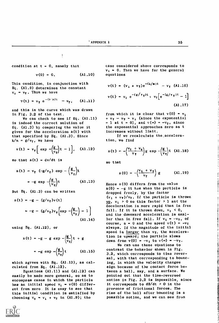
APPENDIX 1 55

condition at t 0, namely that

v(0) = 0.

case considered above corresponds tovi 0. Then we have for the general

(A1.10) equations

This condition, in conjunction withEq. (A1.9) determines the constantvo = VT. Thus we have

v(t) = vT e VT, (A1.11)

and this is the curve which was drawnin Fig. 3.2 of the text.

We can check to see if Eq. (A1.11)is indeed the correct solution ofEq. (A1.3) by comparing the value itgives for the acceleration a(t) withthat specified by Eq. (A1.3). Sincehim = g/vT, we have

v(t) = vT[ exp -(19t 1], (A1.12)v T

so that a(t) = dv/dt is

a(t) vT (-g/vT) exp (L.)tvT

= -g exp -(g-)t (A1.13)VT

But Eq. (A1.3) can be written

a(t) -g - (g/vT)v(t)

-g (g/vT)vT[exp 1]

(Al.14)

using Eq. (A1.12), or

a(t) = -g - g exp -(glt +gT/

-g exp (A1.15)vT

which agrees with Eq. (A1.13), as cal-culated from Eq. (A1.12).

Equations (A1.11) and (A1.12) caneasily be made more general, so as toencompass cases in which the particlehas an initial speed vi v(0) differ-ent from zero It is easy to see thatthis initial condition is satisfied bychoosing vo a vi + vT in (A1.9); the

v(t) = (vi + vT)e-(k/m)t

- v T (A1.16)

v(t) = vi e -(g/vT)ti v4e-(g/vT)t- 1]

(A1.17)

from which it is clear that v(0) - Vi+ VT - VT = VI (since the exponential- 1 at t = 0), and v(o) -vT, sincethe exponential approaches zero as tincreases without limit.

If we recalculate the.accelera-tion, we find

vi + va(t) -( T)g exp -(g-)t (A1.18)

vT VT

so that

a(0) =V+

VT\

) g(A1.19)

T

Hence a(0) differs from the valuea(0) = -g it has when the particle isdropped freely, by the factor(vi + vT)/vT. If the particle is thrownRe, vi > 0 so this factor > 1 and thedeceleration is more rapid than in freefall. If it is thrown down, vi < 0,and the downward acceleration is smal-ler than in free fall. If vi = -VT, ofcourse, a - 0 and the speed v(t) = -vTalways. If the magnitude of the initialspeed is larger than VT, the accelera-tion is upward; the particle slowsdown from v(0) -vi to v(..0) -vT.

We can use these equations tocontrast the behavior shown in Fig.3.2, which corresponds to time rever-sal, with that corresponding to bounc-ing, in which the velocity changessign because of the contact force be-tween a ball, say, and a surface. Wepointed out that the time-reversedmotion in Fig. 3.2 is impossible, sinceit corresponds to dE/dt > 0 in theprepence of frictional forces. Therise of the ball after bouncing is apossible motion, and we can see from

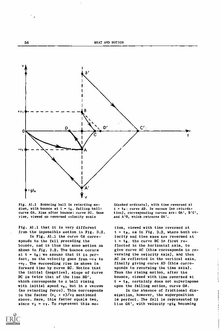
56 HEAT AND MOTION

Fig. A1.1 Bouncing ball in retarding me-dium, with bounce at t - tx. Falling ball:curve OA. Rise after bounce: curve BC. Samerise, viewed on reversed velocity scale

Fig. A1.1 that it is very differentfrom the impossible motion in Fig. 3.2.

In Fig. A1.1 the curve OA corre-sponds to the fall preceding thebounce, and is thus the same motion asshown in Fig. 3.2. The bounce occursat t tR; we assume that it is per-fect, so the velocity goes from -vT to+VT. The succeeding rise is shown inforward time by curve BC. Notice thatthe initial (negative), slope of curveBC is twice that of the line BD',which corresponds to a ball risingwith initial speed vT, but in a vacuum(no retarding force). This correspondsto the factor (vi + v)/vT mentionedabove. Here, this factor equals two,since vi VT. To represent this mo-

(dashed ordinate), with time reversed att ta: curve AD. In vacuum (no retarda-tion), corresponding curves are: OA', B'C',and A'0, which retraces OA'.

tion, viewed with time reversed att - tR, as in Fig. 3.2, where both ve-locity and time axes are reversed att tR, the curve BC is first re-flected in the horizontal axis, togive curve AC (this corresponds to re-versing the velocity axis), and thenAC is reflected in the vertical axis,finally giving curve AD (this corre-sponds to reversing the time axis).Thus the rising motion, after thebounce, viewed with time reversed att tR, certainly does not superimposeupon the falling motion, curve OA.

In the absence of frictional dis-sipation, however, the superpositionis perfect. The fall is represented byline OA', with velocity -gtR becoming

APPENDIX 1 57

+gtR after the bounce. Line B'C' isthe rise after the bounce with timeflowing in the same direction as be-fore the bounce. The reversal of veloc-ity and time at t = tR now gives C'A'and A'0, respectively, and AIO is anexact superposition on OA'.

These equations for the exponen-tial variation of v(t) and a(t) haveseveral interesting aspects. Noticethat according to Eq. (A1.13) the ac-celeration, which at t = 0 is a = -g,the free-fall value, decreases exponen-tially to zero. Hence the terminalspeed, vT, is reached only after an in-finite time. However, exponential de-crease is quite rapid. For instance,e-3P-, 0.05, so according to Eq. (A1.12),when (g/vT) 3, v will already havereached 95% of VT; and when (g/vT)t - 9,v will be within about a quarter of onepercent of VT. These statements can beused to give a quantitative meaning tothe statement in the text that the par-ticle reaches the terminal speed if itfalls "long enough." We notice thatg/vT has the dimension sec-1; so vT/ghas the dimension of time, and can beset equal to a "decay time," denoted T.

VT/g. (A1.20)

Now we can repeat the remarks aboveabout the rate at which v approachesVT, by saying, for instance, that v/vT0.95 when t = 3T.

From Eq. (A1.4), we see that

T = mg/kg - mik, (A1.21)

so that the decay rate depends on themass of the particle and on the coef-ficient of proportionality, k, betweenretarding force and speed, but not onthe free-fall acceleration. The larger7 is, the slower v approaches vT. Equa-tion (A1.17) thus shows that the ap-proach to vT becomes slower (also, ofcourse, vT increases, as shown byEq. (A1.4)), as the retarding forcecoefficient, k, decreases. This wouldbe expected intuitively, but it mightnot have been so obvious that r alsoincreases for more massive particles.

This effect, and the associated rela-tion, vT « m, would not have been atall surprising in the Aristotelianview of motion, according to whichheavy objects fall faster than lightones. We can see from our discussionprecisely how Galileo's refutation ofthe Aristotelian point of view dependson idealization to the situation inwhich resistance due to the medium isabsent.

We know that the resistance of-fered by the medium depends on thesize and shape of the object, so weexpect that k has this dependence also.Hence we are dealing with an examplein which the particle model cannot beexpected to be complete. Thus, k shouldalso depend on the medium. The retarda-tion effect of a medium is usually ex-pressed in terms of its viscosity. Atthis point we need concern ourselvesonly with its dimensions, namely dynesec/cm2. So if we denote viscosity byn, we have the dimensional equation

n 4 dyne sec/cm2.

But from Eq. (A1.2)

k 4 force/speed 4 dyne sec/cm.

(A1.22)

(A1.23)

Hence, comparing Eqs. (A1.22) and(A1.23), we can write

k a of (A1.24)

where f is a length associated withthe object. Inserting this in Equation(A1.21), we see

7 mina. (A1.25)

Thus the retardation effect, expressednow in terms of T, has been separatedinto three factors: m and f, which re-late to the object, and n, which de-pends only on the medium. We note,finally, that the remark that "f is alength associated with the object" can-not be made more explicit without spec-ifying the detailed size and shape of

58 HEAT AND MOTION

the object. For a particular object, acomplicated calculation would be re-quired to find exactly how it is re-tarded by the medium. The result r.1 thecalculation would then give a numberwith the dimension of length. This num-ber would not necessarily be simplyrelated to the size of tho object. Forinstance, we would expect intuitivelythat a thin square plate of side awould have a shorter r (and lower vr),than a sphere of diameter a, if bothhad the same mass. That is, the platehas a lower terminal speed, and reachesit sooner, than the sphere. Hence(plate should turn out to be larger than

sphere ,for the same a and m.

On the other hand, we can alsocompare T for spheres of the same mate-rial, but different radius r. We seethat since m = pV, where p is the den-sity and V the volume, V - (4e3)r3,we have

T LL pr3/0.,94(4, or T a pr2/11 (A1.26)

shore wo have assumed that Isphere is

proportional to r. Hence T increasesrapidly with the size of the sphere.

One final aspect of these equationsshould now be mentioned. In going fromEq. (A1.1) to Eq. (A1.3), a term wasneglected which should be included.The term -mg in Eq. (A1.1) is theweight of the particle in a vacuum; ina medium its apparent weight will beless, due to the buoyant force, so inEqs. (A1.3) and all those that follow,m should be replaced by m', where

Mi = m My, Mm pmV, (A1.27)

where mm is the mass of the amount ofmedium displaced by the particle; pmis thus tne density of the medium.Hence, in Eq. (A1.26), the density ofthe particle should be replaced by

P' ° P Pm.

Appendix 2 FRICTIONALMECHANICAL

We would like to calculate the rate,dE/dt, at which mechanical energychanges as a result of forces appliedto a particle, and to show that therate is always negative for frictionalforces. If we write Eq. (3.1) in termsof Cartesian components of the speed,we have

K = im(vz2 + Vy2 + Vz2). (A2.1)

This can be written more compactly,with the summation notation, if we in-troduce numerical indices: vi,

vy - v2, vz - v3. Then (A2.1) becomes

3

K = im vie

We can also write K in terms of themomentum, p, defined by

(A2.2)

so that

P2

p m v,

3

pi2=

m2 vi2, (A2.3)

i=li=1

and therefore

K(pi) - (1/2m) 1] pie .

i-1

(A2.4)

If we also use numerical indices forcomponents of the position vector, orx ri, y r2, z r3, then we canwrite the dependence of the potentialenergy V on the position vector r as

V(r) V(x,y,z) - V(r1,r2,r3) V(ri).So we can write for the mechanical en-ergy,

E(pi,ri) K(pi) + 11(ri). (A2.5)

Now E does not depend on t explic-itly, so in order to calculate dE/dtwe must use the partial derivativechain rule, which takes into account

59

FORCES ANDENERGY

the implicit dependence of E on tthrough the time dependence of pi andr 3' We therefore have

3

dE iraE va2.0 RE )(dr91dt (Aapt)kat kar dt

(A2.6)

According to (A2.5), E depends on pionly through K, and on ri only throughV; so

aE/aPi aK/api; aEari aV/ari.

(A2.7)

From (A2.4), we have

aK/api (1/2m) 2pi = pi/m vi.

(A2.8)

Also, the potential V is related to aF(c)-conservative force F by

Fi") -8V/ari. (A2.9)

Finally, the term dri/dt is simply vi.We can therefore factor out vi fromeach of the terms in A2.6, with theresult

3

dE 22(1121.Flo)

(A2.10)Viati

dti=1

Tfie total force Y on the particlemay have a nonconeervative part Y, aswell as a conservative part; that is,

P(c) + Ye or Y") Yt

But according to N-II, Eq. (A2.8),

m dVdt di-Vdt, so

dpi/dt - Fi") Fig.

Therefore, from (A2.10),

(A2.11)

60 HEAT AND MOTION

3

dE/dt 2] vi Ey' = v F' (A2.12)1 =1

where the last equality expresses theresult using the vector dot-product.Hence the mechanical energy is constantunless nonconservative forces act onthe particle. Frictional forces arenonconservative, and also, are alwaysdirected opposite to v. If we denotefrictional forces by 7, as in the text,then

dE/dt = v . f < 0. (A2.13)

Note that this is a result for thetotal mechanical energy. It is notnecessarily true that dK/dt < 0 whenfrictional forces act; that is, fric-tional forces need not slow down theparticles. In orbital motion, for in-stance, as with artificial earth satel-lites, when frictional forces act,dK/dt > 0 and the particle speeds up.But the orbit corresponding to a higherspeed has a smaller radius, so dV/dtdecreases. The magnitude of dV/dt islarger than that of dK/dt, so statedby (A2.13), dE/dt is negative.

Appendix 3 ZERO TEMPERATURE ON THEGAS-THERMOMETER SCALE

Despite its modest title, this appen-dix has a rather ambitious aim. Westart with the question: What is thesignificance of a temperature denotedby Tg 0? Using the analysis of thisquestion, we proceed to the statementof a very general result, the unattain-ability of "absolute zero," which canbe given a precise meaning in terms ofour abstract definition of temperature,without necessarily referring to anyspecific temperature scale. Up to thispoint, we have bean considering macro-scopic systems exclusively. Now, usingthis result, we are able to examinethe thermal behavior of certain remark-able atomic systems. We find that theseatomic systems possess thermal proper-ties not shared by any macroscopic sys-tem. Finally, we are able to show howthe concept of temperatur' can be gen-eralized in a surprising way, so as todescribe the unusual thermal behaviorof these special atomic systems.

A.1 ABSOLUTE ZERO

The same standard state, namelymutual therms? equilibrium among ice,water, and water vapor, is used in de-fining the Celsius scale, the gas ther-.aometer scale. and the ideal gas scale.On the Celsius scale, defined byEq. (4,1), the standard state is as-signed the temperature zero, that is,Ts = 0° C. Both the other scales aredefined by Eq. (4.5), and since P(Te)= Po, this gives To = To °K. In thegas-thermometer scale, the constant Tovaries with the gas used," while inthe ideal gas scale, To has a universal

solo 'moral, to also varies with temperature,so the term %outset" right spear to be a ells-sorer. however, the vartatios is sot large, overtemperature :asses which are sot extremely wide.Because of this slow variatios of to with tem-perature, it may be regarded as at least approx-imately tosslast, especially if high accuracyis sot derarded of gas thermometer temperaturemeasuresests.

61

value, independent of the gas used (intne limit of low pressures), and alsoindependent'of temperature. In boththe gas-thermometer and ideal gasscales, the state for which Tg ... 0,

would correspond to gero measured pres-sure, in a gas thermometer which origi-nally was filled to pressure Pc, in thestandard state.

We will see later that the thermalequilibrium state identified by Tg - 0does have a special significance. How-ever, we cannot deduce anything aboutthis state from the properties of agas-thermometer scale. Tho reason issimply that all real gases liquefywhen the temperature is low enough, ata finite pressure, P > 0. When thishappens, the system (homogeneous massof gas), changes its form, and sepa-rates into two phases, a liquid and itsvapor. Once the liquid has formed,Eq. (4.5) no longer relates pressureto temperature, since it ;tribesonly the properties of a homogeneousmass of gas, and not the f, 1)avior of a

vapor in equilibrium wit .: rs liquidphase.

Now the ideal gas does notrefer to any real gas, t verthe-less, it is just as impubbluru to de-duce any properties of the state Tg = 0from this scale, as from the gas-ther-mometer scale. The definition of theideal scale requires a sequence of gasthermometers tilled with a real gas,each using a smaller pressure Po inthe standard state. But when the tem-perature is so low that all gases haveliquefied, we cannot carry out thislimiting process, and so cannot definethe ideal gas scale. Hence, there isno meaningful way to assign the tem-perature Tg = 0 to any thermal equilib-rium state. Similarly, there is no wayto assign a negative value of T. to anythermal equilibrium state, since we can-not conceive of measuring a negativepressure in a gas thermometer.

These arguments lead to the fol-

62 HEAT AND MOTION

lowing trap, which we must be carefulto avoid. We have established a temper-ature scale on which negative tempera-tures, Tg < 0, are meaningless. Onthis scale, the state with Tg - 0 ietherefore colder than any other, sinceall other possib, states have highertemperature. But we have also shownthat it is meaningless to assign thetemperature Tg ° 0 to any thermal equi-librium state. We might therefore betempted to conclude that no such "cold-est" thermal equilibrium state can ex-ist. Such an argument would be incor-rect, because our argument rests onthe properties of the ideal gas scale.Conceivably, there could be other tem-perature scales, with different prop-erties, for which the argument abovebreaks down.

Unfortunately, at this point wecannot discuss this question in gen-eral, that is, without an explicit con-nection with a specific temperaturescale, such as the gas-thermometer orthe ideal gas scale. However, it ispossible to state the results of sucha discussion. In the first place, wecan define what we mean by a "coldest"state, without reference to any par-ticular temperature scale. A coldeststate would have the property, thatany other state could be reached fromit by the dissipation of mechanicalenergy. It is possible to conclude,from observations which we cannot de-scribe here, that:

Starting with any thermal equilib-rium state of any system, it is im-possible to reach such a coldeststate, by any means whatever.

This statement is usually called theThird Law of Thermodynamics.

From this statement we can con-clude that there is no lower limit tothe temperature which can be assignedto attainable states, whatever the tem-perature scale eaplcyed. This Pict canbe incorporated into any temperaturescale, by adjusting its origin so thatall attainable states have positivetemperature, and the unattainable cold-

est state has zero temperature. We willcall temperature scales which have beenadjusted in this way, Third-Law temper-ature scales. We see, for instance,that Tg is such a scale, while Te isnot. If we wish to discuss temperatureon a Third-Law scale without specify-ing whether it is Tg or some othersuch scale, we will use the notationTut. Since the identification of thecoldest state, Tut - 0, does not referto any specific temperature scale, bulrather to all scales on which attain-able states have positive temperature,the coldest state is often referred toas "absolute zero." The Third Law ofThermodynamics, correspondingly, maybe described as asserting that "abso-lute zero is unattainable."

A.2 NEGATIVE TEMPERATURE

We see that if we had fallen intothe trap discussed above, we would havereached the correct conclusion, butfor the wrong reasons. We should nowexamine our earlier conclusion thatnegative temperatures, T1 < 0, aremeaningless. if we examine the way inwhich we defined Third-Law scales, Tin,it is easy to so see that states forwhich T111 ' 0 cannot be colder thanthe absolute zero state, since "colderthan coldest" is self-contradictory.But this does not necessarily meanthat no states exist, for which T111< 0. It does mean, that like all otherstates, s9ch states must be hotterthan the state at absolute zero,

Tit: 0.

Now it is easy to see that if:uch "negative T1/1" states do exist,they cannot be found in every thermalsystem. In particular, they could notbe attained by any system which can beput into thermal equilibrium with agas thermometer. For if this were pos-sible, the temperature could be meas-ured on the Ts scale, and negative tem-peratures are certainly impossible onthat temperature scale. We are thusled to consider whether thermal sys-tems can exist, such that because of

APPENDIX 3 63

their physical nature they cannot beput into thermal equilibrium with agas thermometer.

It might seem obvious that theanswer to this question is "no." Thiswould indeed be the correct answer ifwe restricted uurselves to macroscopicsystems, that is, to systems which arelarge enough to be manipulated, or, inother words, systems which can bepicked up and moved about. In princi-ple, such manipulation could includearranging thermal contact with a gasthermometer, or at least with someother thermometer which could be com-pared with a gas thermometer in a sec-ond operation. But this sort of manip-ulation is impossible, even in princi-ple, for systems on the scale of atomsand nuclei. Hence it is on that scaleof size that we must seek for thermalsystems whose temperature cannot bemeasured on the Tg scale.

It is by no means obvious thatsuch states, for which Tg cannot bedefined, can be found even on theatonic scale. After all, every macro-scopic objact which we put into ther-mal equilibrium with a gas thermometeris itself an assemblage of atoms, andin this sase, an "atomic system." ItWAS therefore a remarkabl*: event when,about 1950, Purcell, Ramsey, and Poundreported the existence of an atomicsystem that had a measurable tempera-ture which could not be directly re-lated to the Te scale. Their reportwas based on observations they hadmade on the interaction of lithium flu-oride (LiF) crystals with magneticfields. This interaction occurs be-cause the nuclei in LiF crystals havemagnetic moments. The magnetic fieldcan supply energy directly to the sys-tem of nuclear magnetic moments, inmuch the stale way that mechanical en-ergy can be supplied to the crystal asa whole.

The first conclusion that couldbe drawn from the experiments of Pur-cell, Ramsey, and Pound, was that thenuclear magnetic moments could be re-garded as a thermal system that was inrather poor thermal contact with the

crystal as a whole. The temperature ofthe system of nuclear magnetic moments(we will refer to this system by thesymbol N), could be measured magnetic-ally, on a scale we will denote TR.The temperature of the crystal itself(we will refer to this system by theletter L), could of course be measuredon Tit, since L is a macroscopic system.Thermal contact between systems N andL was investigated by experimentswhich can be described very roughly asfollows: In the first stage, a.crystalof LiF is in thermal isolation fromits surroundings, with no magneticfield applied. According to our basicdefinition of thermal equilibrium, sys-tems N and L must arrive at a state ofmutual thermal equilibrium. This statewill be recognized by the fact thatTe(Ne) and Tg(Le), which are respec-tively the temperature of the nuclearmagnetic moment systems, measured onthe magnetic scale, and the tempera-ture of the crystal, measured on thegas-thermometer scale, are both con-stant. The subscripts e on the symbolsfor the system emphasize the fact thatthis is an equilibrium state. Now themagnetic field is applied, and thesystems are momentarily in the secondstage of the experiment. The tempera-ture of the system N immediately jumpsto a new value, Tu(N2), while the tel.-perature of system L is uncharged,since no mechanical energy was dissi-pated in that system. The momentarysecond stage is followed by the thirdstage, which takes several minutes.During this stage, the temperatures ofboth systems change slowly, showingthat they are in thermal contact; butsince the changes take place slowly, werecognize that the thermal contact ispoor. Finally, the fourth and laststage of the experiment is reached, inwhich both systems have reached new con-stant temperature, To(Nei) and Te(Le'),showing that they are once again in mu-tual thermal equilibrium. However, aswe would expect, the new equilibriumstates, denoted N.' and 1,4's are dif-ferent from those in the first stage,N. and Ls.

64 HEAT AND MOTION

The series of stages in this ex-periment is exactly analogous to ob-servations that could be made with thearrangement of Fig. 4.1, using macro-scopic systems exclusively. If theplate on top of the bell jar is madeof wood, a system on the plate wouldbe in poor thermal contact with thependulum bob inside the jar. Applyingthe magnetic field to the crystalwould correspond to suddenly changingthe temperature of the system on thewooden plate. Because of the poor ther-mal contact there would be no corre-sponding jump in the temperature ofthe pendulum bob, which is the analogof the crystal in the LiF experiment.The third and fourth steps of the ex-periment would proceed just as above,with the temperatures of the system onthe plate, and of the pendulum bob,both changing and ultimately reachinga new thermal equilibrium.

Now in either case, the LiF ex-periment or its completely macroscopicanalog, we can easily deduce which ofthe initial systems was hotter in themomentary stage two, by simply compar-ing the initial and final . quilibriumtemperatures of just one of the sys-tems, namely the crystal in the LiFexperiment, nr the pendulum bob in themacroscopic analog. If Tg(Le') >Tg(Le), for instance, then the crystalwas warmed by its contact with the sys-tem of nuclear magnetic moments, sosystem N must have been heated by theapplication of the magnetic field, an.1was therefore hotter than L during themomentary stage two and thereafter,until the final equilibrium wasreached. Now with the macroscopic ana-log experiment, this sort of discussionwould be unnecessary, since temperaturesof both the system on the plate and ofthe pendulum bob can be measured onthe scale T 41. Ts and thus compared di-

rf4tly. In the LIF experiment, on Cieother hand, the temperature of systemN can be measured directly only onscale Ts. Now in stages ont and fourof the experiment, systems N L arein thermal equilibrium, so IWO isequal to Tg(Lo) and Ts(N40) is equal

to Tg(Le')." However, in stage two ofthe LiF experiment, system N is not inthermal equilibrium with system L, sothe comparison between Tg(Le) andTg(Le.) is the only way of determiningwhether Te(N2) is hotter or colderthan Tg(Le),

Now as long as we are dealingwith macroscopic systems, we would ex-pect to find that however large theinitial increase of temperature of thesystem on the plate in stage two ofthe experiment, we can always prepareanother system that is even hotter.For instance, if the system on theplate has temperature, say, (T1)2 instage two, we can prepare another sys-tem with temperature (rg)e t 1. Thisother system, since it is hotter thanthe system on the plate, will have itstemperature lowered if it is broughtinto contact with the system on theplate. That is, there is no "hottest"temperature on the Tg scale.

In remarkable contrast to thissituation, it was found in experimentson LiF crystals that, by suitable in-teractions with magnetic fields, itWho possible to prepare system N ofnuclear magnetic moments in stateswhich were hotter than any state of amacroscopic system. That is, it couldbe shown that special states, which wewill denote Nelt, could be preparedwhich had the property that arg macro-scopic system, whatever its thermalequilibrium state, would be warmed onbeing brought into thermal contactwith that state. Of course, this con-clusion could only be reached indi-rectly, since it is clearly impossibleto carry out experiments on an unlim-ited number of macroscopic systems in

"the equality of these two pairs of teapera-tures does mot secessarily seas that they havethe same nuserical value, only that they are as-sisted to thermal equilibrius states le mutualequilibrium. Is the same tease, the tesperature32'F 10 'equal" to the temperature 0°C, sltetwzi,hthe n4merical values ea the to scales are dif-fittest. The restos is that both tesperatures re-fer to the same thermal equilibrium state,namely the comma standard state oe the Celsius,gas-thersonetet, aid ideal sits scales.

APPENDIX 3 65

a finite length of time. Nevertheless,this was an inescapable conclusionfrom the experiments which were per-formed.

Another way of stating this con-clusion is to say that such a specialstate N2* is hotter than any thermalequilibrium state of any macroscopicsystem. The question arises, whetherit is possible to assign to such astate a temperature Ti//(N2*) on aThird-Law temperature scale. SinceT///- 0 defines the unattainable cold-est state, and positive Tuicorrespondsto ordinary thermal equilibrium statesof macroscopic systems, we have avail-able only negative temperatures, T111< O. But now there is no bar to usingnegative temperatures, as there was onthe Tig scale, since as we have seen, astate like N2* is not in thermal equi-librium with any thermal equilibriumstate that has a temperature on the T1scale. So we have finally arrived at ameaning for negative temperatures on aThird-Law scale, at least for certainspecial atomic systems like that ofthe nuclear magnetic moments in a LiFcrystal. They correspond to "superhot"states which are hotter than any stateswith positive temperature on a T111scale.

One question remains - how shallwe assign numerical values to the tem-pe..tures of two different "superhot"states? A consistent convention is toassociate "hotter" with larger alge-braic value of the temperature, ratherthan larger magnitude. Thus, for in-stance, a state with T111 k. -100°K is

hotter than the state with Ttil-1000°K. We can now arrange all states,both "normal," corresponding to macro-scopic systems, and "superhot," in oneconsistent order. Starting with the(unattainable) coldest state with Tin0, increasingly hotter states have

larger and larger temperature values,which approach the limit Till 4*.

States hotter than this limit are "su-perhot"; their temperatures start fromthe limit Tilt and increasinglyhotter "superhot" states have tempera-tures which increase in algebraic

value, approaching T111 a 0, but frombelow. This limit is the "absolutelyhottest" state; like the "absolutelycoldest" state, it is unattainable.There are now two states correspondingto "absolute zero," depending onwhether the approach is from positiveor negative temperatures; the ThirdLaw states that neither of these statesis attainable.

The convention we have describedfor handling negative Third-Law tem-peratures is the only one that leavesordinary temperatures Ts unchanged. Itis rather clumsy, however, since thesame state is represented by eitherT/// t.m, or TIJI and also T111

0 represents two vastly differentstates, depending on the direction inwhich it is approached. A simple modi-fication of the scale produces a dras-tic change in conventional temperaturescales, but it eliminates these diffi-culties. We introduce a scale denotedR///, defined by the negative recipro-cal of T111 ,

R111 -(1 /Till ).

The relation between R111 and Till is

shown in Fig. A3.1. The curves in thefigure are hyperbolas, according tothe definition of R111, and the arrowson the hyperbolas indicate the direc-

obsolutely hottest"

Of IPsupedlot

R -(1/Tin)

notreol

.1 IPabsolutely coldest

Fig A3.1 Temperatures on the scale Amplotted as a fuactioa of teaperatures onthe scale Tilt .

66 HEAT AND MOTION

tion corresponding to "hotter." On thescale 11/11, the "absolutely coldest"state has RI/1 - and the hottestnormal state is RH/ 0, approachedfrom below, so all normal temperatures,appropriate to macroscopic systems,are negative. All "superhot" tempera-tures are positive, the coldest ofthese being Rin 0, approached fromabove. The "absolutely hottest" stateis R111 a. +0*.

It is not likely that the R/11scale, which clarifies the relationbetween normal and "superhot" tempera-

tures, will ever be commonly used.How,wer, since the original experi-ments on LiF were performed, manyother atomic systems have been foundwhich can also attain "superhot"states. Furthermore, such systems areno longer merely laboratory curiosi-ties. Their "superhot," or, as theyare commonly called, "negative temper-

ature" (on a T111 scale), states makepossible the operation of masers foramplification of minute microwave sig-nals, and also lasers, which produceintense beams of coherent light.

Appendix 4 INTERCOMPARISON OFTEMPERATURE SCALES

As we have pointed out, every systemwhich is chosen to serve as a thermom-eter, and indeed, every thermometricproperty of such a system establishesits own temperature scale. There are agreat many thermometric properties ingeneral use, besides the liquid-in-glass thermometers we have described.A common type is based on the proper-ties of a coiled strip, made fromstrips of two different metals weldedtogether. The two metals are chosen sothat they expand at different rateswhen they are heated. Then a coil madefrom such a bimetallic strip will ro-tate about a fixed point to which oneend is attached so that it cannotmove. The angle of rotation of apointer attached to the other end of

the strip then serves as a thermomet-ric property. Oven thermometers areusually of this kind.

The electrical resistivity ofmetals, alloys, and semiconductorsvaries with temperature, and so can beused as a thermometric property. If,in a loop made of wires of two differ-ent metals or alloys, the two Junc-tions are at different temperatures,an electrical voltage is developed inthe loop, and the magnitude of thisvoltage can serve as a thermometricproperty.

Now this profusion of temperaturescales leads to difficulties, whenevertwo temperatures are to be compared,which have been measured using differ-ent thermometers, say A and B. If thescale appropriate to each is used,then it can happen that two thermalequilibrium states can have the same

numerical value of the temperature,TA TA, but still not be in mutualthermal equilibrium. Or it can happenthat one thermal equilibrium state canhave two different numerical values oftemperature, Ti # when measuredwith two different thermometers.

These situations can arise as

67

follows: Suppose, to take a concretecase, we consider a mercury-in-glassthermometer (A), and a platinum resist-ance thermometer (B). When both are inequilibrium in the standard state ofthe Celsius scale (0°C), the length ofmercury in the capillary is L(0°C) cm,and the resistance of the platinumwire is R(0°C) ohm. When both are inequilibrium with water boiling atstandard atmospheric pressure (P760 mm of Hg), the corresponding val-ues are L(100°C) cm and R(100°C) ohm.Now suppose that, in equilibrium witha third state, we observe that thelength of mercury in the capillary hasexpanded to 0.40 of the distance fromL(0°C) to L(100°C). That is

L(TA) L(0 °C) + 0.4011,(100°C) L(0°C)I

(A4.1)

We would be entitled to denote thistemperature as TA 40°(A), since ithas been determined from thermometer(A), mercury-in-glass. Now in equilib-rium with the same thermal equilibriumstate, we might find that

R(TA).. R(0 °C) + 0.4101(100°C) R(0°C)),

(A4.2)

so that we would assign to this state,Ti la 416(B), corresponding to thermom-eter (B), platinum resistance. Thereason for the discrepancy is that thedensity of mercury between 0°C and100°C does not vary in exactly thesame way as the resistance of platinum,between the same two temperatures.

In order to avoid the confusionabout numerical values of temperatureexpressed in Eqs. (A4.1) and (A4.2),and its further compounding when otherthermometers are considered as well,careful measurements with gas-thermom-eters in standard laboratories allover the world are used to establish ascale which is adopted as standard by

68 HEAT AND MOTION

international agreement. In terms ofthis international Celsius scale, meas-urements with any chosen thermometercan be compared with those of anyother. For instance, it might be foundthat the state described above, forwhich TA 40°(A) and Ts 41 °(B), hasthe temperature Te 40.5°C on the in-ternational Celsibs scale. The pointon the capillary, which is describedby Eq. (A4.1) would not be marked "40,"

but rather, "40.5," and we would saythat this thermometer has been cali-brated against the international Cel-sius scale. After this calibration pro-cedure has been carried out for anyparticular thermometer, that thermom-eter can be used to measure tempera-ture on the Celsius scale, even thoughthis standard scale, and that definedby the particular thermometer chosen,will in general be different.

Appendix 5 INTERNAL DEGREES OF FREEDOMAND THE ATOMIC MODEL

The amount of detail that we have gonethrough in this discussion leading tothe conclusion that matter possessesinternal degrees of freedom may appearstrange to the average reader, who hasundoubtedly been raised to accept theexistence of atoms and molecules as anarticle of faith. He or she is there-fore perfectly well aware that theforce Fu introduced in section 6.1"obviously" comes from random colli-alone of the particle with the atomsor molecules of the fluid in which itis in suspension. We certainly do notwish to challenge this faith in theexistence of atoms and molecules, butwe do wish to examine it rather moreclosely than is sometimes done. Ourargument was designed to show that thenecessity for postulating an internalstructure follows directly from obser-vations on purely macroscopic behavior.For such a conclusion to be convincing,the discussion on which it was basedcould not rely on any assumptions aboutinternal structure; otherwise the rea-soning would be circular. Furthermore,the characteristics of the internalstructure (tan also be deduced frommacroscopic observations. Some aspectsof this deduction are described insections 6.1 and 6.2.

After all, belief in the existenceof atoms is not exactly a novelty. Itdates back well over two millenia; ithad its adherents among the classicGreeks and Romans, But during thisancient period (which lasted, in fact,well into the eighteenth century),this belief had no real foundation inthe known behavior of nature. It wasin the realm of metaphysics ratherthan physics. And it does not leavethat realm simply by becoming absorbedinto everyday thinking if there is lit-tle conception of how it is related tothe understanding of natural phenomena.

As a matter of fact, the naiveversion of atomic theory that was de-

69

veloped during the eighteenth andnineteenth centuries, in which the at-oms and molecules are simply Newtonianparticles, is inadequate for under-standing many kinds of phenomena whichit should be able to explain. The es-sential distinction between the macro-scopic and atomic levels of size wasmade at the beginning of section 5.2.It was pointed out there that the mac-roscopic degrees of freedom are alwaysadequately described by Newtonian me-chanics, while the degrees of freedomassociated with the internal structureof matter must be described by quantummechanics. The nature of this distinc-tion was clearly realized only about1925 when quantum mechanics was devel-oped in two independent but equivalentformulations. Before then, attempts toapply Newtonian mechanics to phenomenaon the level of atomic size requiredvarious revisions of classical mechan-ics for different problems such asatomic spectra, atomic collisions, nu-clear transmutations, electrical prop-erties of solids, and these revisionssometimes appeared to have little con-nection with one another. Many physi-cists who had been trained in the nine-teenth century, before much attentionhad been paid to these problems, there-fore had little faith in the validityof the naive atomic theory. Its longhistory as essentially speculativephilosophy, largely divorced from arelation to natural phenomena, tendedto reduce what little faith they had.Their attitude towards attempts to giveit a firm connection with observationwas that a model was being devisedwhich was being diverted from the es-sential behavior of matter by trivi-alities. They could point, as an exam-ple, to Aristotle's model for motionwhich had been led astray by regardingfriction as the essential feature ofmotion, rather than equilibrium, withconstant vet city. This attitude was

70 HEAT AND MOTION

well expressed by Mach, who wrote (in1915), "I do not consider the Newton-ian Principles as a completed and per-fected thing, yet in my old age, I canaccept the theory of relativity justas little as 1 can accept the existenceof atoms and other such dogma." In acertain sense, Mach's attitude wascorrect, since the naive atomi...t theory

of which he was writing was certainlywrong. But in another sense, the judg-ment of Mach and the others who sharedhis point of view, many of whom hadmade great contributions to physics,was bad. What they regarded as one ofthe blind alleys we mentioned in sec-tion 1, turned out to be a broad ave-nue whose exploration led to the mostcoherent and encompassing picture ofnature ever devised. But in one ironi-cal sense, the doubters were right,after all. The difference between thenaive atomic theory, which Mach re-jected, and quantum mechanics, is cer-tainly not trivial. The quantum-mechan-ical behavior of the internal degreesof freedom of matter can be very un-like that of Newtonian mass-points.For instance, we may inquire as to thelocation of an electron in an atom.The model of which Mach was complain-ing would answer in terms of a pointcharge rotating about a nucleus. Incontrast, quantum mechanics will speakof probabilities, rather than a well-defined location. And the probabilitiesare givea in terms of wave functions,which have finite values everywhere,not just at a geometrical point. Soquantum mechanics agrees with Mach, inrejecting the mass-point as a suitablemodel, in general, for the internal de-grees of freedom.

As a result, it Is not really ac-curate to speak of the ultimate tri-umph of the atomic theory, more than

two thousand years after its firstpronouncement. The lorg dispute betweenthose who asserted that matter was madeup of a continuum, and those who as-serted that it had an internal struc-ture of indivisible parts separated byvacuum, seems to have been resolved infavor of the latter point of view. Butthe atoms of the structure we now rec-ognize bear little resemblance to thosedescribed by Lucretius: "Bodies of ab-solute and everlasting solidity . . .

absolutely solid and unalloyed." Andthe void between atoms is far fromfeatureless: it is the seat of gravi-tational, electric, and magneticfields. Therefore, while quantum me-chanics is a descendant of primitiveatomic theory, it is better describedas a remarkably successful fusion ofthe atomic and continuum points ofview.

It should not be imagined, how-ever, that quantum mechanics is compe-tent to answer all questions about theinternal degrees of freedom of matter.The structure of nuclei is still anunsolved problem, and even some phe-nomena on the atomic level, which canbe described quite simply, have notbeen accounted for in detail. One ofthe outstanding examples is the exist-ence of the different phases of matter.A collection of atoms or molecules cantransform from a gas, which fills thevolume of its container, to a liquid,which has a definite volume at a fixedtemperature, but whose shape is stilldetermined by its container, to asolid, which has a definite sire andshape, in which the atoms are arrangedin a regular three-dimensional pattern.The processes by which these transfor-mations occur are still imperfectlyunderstcod.