“It always seems impossible until it's done.”

Nelson Mandela

ii

Acknowledgments

It is with a huge pride and happiness that I have finished my dissertation. After a long journey to conclude

my study, it is now important to make some acknowledgments to the persons who supported me in this project.

I would like to express my heartfelt gratitude to my supervisor, Professor Luís Aguiar-Conraria, for his

invaluable guidance, patience, dedication and encouragement. His valuable knowledge inspired me to continue

forward to complete this dissertation.

I also want to extend my sincere gratitude to the University of Minho and the School of Economics and

Management, especially to all the professors from my Master in Monetary, Banking and Financial Economics that,

directly or indirectly, helped me with this research.

A special thanks to all my family and specially my parents, who have always supported me unconditionally

in all hard times with a massive love and encouragement.

I would like to thank to my beloved wife, who always supported me, giving me strength, inspiration, courage,

kindness, affection and a huge love to continue bravely forward.

Finally, my sincere thanks to all my colleagues and special friends for all the academic and funny moments

we have shared during two years and will continue to share. Their support and friendship was always very important

and precious for me.

To all, my deepest and sincere thank you.

iii

Abstract

Purpose – The purpose of this research is to analyze and extend the study of contagion for BRICS Emerging Stock

Markets in the context of the last two international financial crises: the Lehman Brothers Bankruptcy Crisis and the

European Sovereign Debt Crisis. We investigate changes in the relationship and the co-movements between BRICS

markets in response to international shocks that are originated in advanced markets like USA and Europe.

Methodology approach – Employing data of daily stock market indices of BRICS countries, this research tests

for contagion, examining the interactions and characteristics of price movements of BRICS stock markets by

applying a three-step Methodology: cointegration analysis, causality and VECM/Gonzalo-Granger statistic and

variance decomposition methodology on stock returns as a measure of perceived country risk.

Findings – The results exhibit that both long-run cointegration relationships and short-run Granger causality

relationships patterns exist between BRICS stock markets. Furthermore, these relations have drastically changed

(amplified) during turbulent periods compared with tranquil period, pointing towards the occurrence of contagion

phenomenon among BRICS markets during the last two crises. These results suggest that the benefits of portfolio

diversification were significantly decayed during both crises and, consequently, diversification was not beneficial

during either crisis.

Implications – The findings imply an increasing degree of global market integration due to quick dissemination

of global shocks originating from the USA and the Euro Zone, and swift recovery which can be attributed to the

increased resilience, consistent with the moderated level of domestically driven risk in the BRICS markets.

Moreover, the results bring major implications for international portfolio diversification and policy makers, since

these markets serve as an important alternative investment destination for global portfolio diversification.

Furthermore, changes in the USA and the Euro Zone indices affect BRICS stock markets in the short-run, which

implies that these markets may act as a leading indicator for investing in BRICS markets.

Keywords: Financial Contagion, BRICS Stock Markets, VAR Models, Financial Crises.

iv

Resumo

Objetivo - O objetivo desta pesquisa é analisar e estender o estudo do contágio para os Mercados Emergentes

dos BRICS, no contexto das duas últimas crises financeiras: a crise originada pela falência do Lehman Brothers e

a crise das Dívidas Soberanas na Zona Euro. São analisadas as mudanças no relacionamento e os movimentos

nos mercados de ações dos BRICS em resposta a choques internacionais provenientes de mercados desenvolvidos

(EUA e a Europa).

Metodologia - Utilizando os dados diários dos índices de ações dos BRICS, o contágio é testado, examinando as

interações e as características dos movimentos de preços destes mercados, aplicando uma metodologia em três

passos: análise da cointegração, causalidade e estatística VECM/Gonzalo-Granger e a metodologia de

decomposição da variância para os retornos de ações como uma medida de perceção do risco país.

Resultados - Os resultados exibem as relações de cointegração de longo prazo e os padrões de relacionamento

de causalidade de curto prazo entre os BRICS. Estas relações foram fortemente amplificadas durante os períodos

turbulentos em comparação com os períodos tranquilos, apontando para a ocorrência do fenómeno de contágio

entre os BRICS durante as duas últimas crises. Revelando assim, uma significativa deterioração dos benefícios de

diversificação em ambas as crises e, consequentemente, uma diversificação pouco benéfica para os investidores.

Implicações - As conclusões inferem um crescente grau de integração global dos mercados devido à rápida

disseminação de choques globais originários dos países desenvolvidos, assim como, uma rápida recuperação que

pode ser atribuída ao aumento da resiliência, consistente com o nível moderado de risco nacional dos BRICS. Os

resultados trazem importantes implicações para a diversificação de investimentos e para os decisores políticos,

uma vez que, os mercados de ações dos BRICS servem como um importante destino de investimento alternativo

para a diversificação de portfolios globais. Evidenciam também, que alterações nos mercados de ações americanos

e europeus afetam os BRICS no curto prazo, o que sugere que estes mercados podem atuar como um indicador

de liderança para o investimento nos mercados de ações dos BRICS.

Palavras-chave: Contágio Financeiro, Mercado de Ações dos BRICS, Modelos VAR, Crises Financeiras.

V

Contents

Acknowledgments .......................................................................................................................... ii

Abstract ........................................................................................................................................ iii

Resumo ......................................................................................................................................... iv

List of Tables and Figures ............................................................................................................ vii

List of Abbreviations.................................................................................................................... viii

1 Introduction ................................................................................................................................ 1

2 Literature Review ........................................................................................................................ 4

2.1 Contagion Phenomenon: Definition, Theories, Transmission and Measurement......................................... 4

2.1.1 What is Financial Contagion? ............................................................................................................ 5

2.1.2 Causes and Transmission of Contagion ............................................................................................. 7

2.1.3 Contagion: Testing and Measurement ............................................................................................... 9

3 Data & Methodology ................................................................................................................ 12

3.1 Data ...................................................................................................................................................... 12

3.1.1 Variable Transformation .................................................................................................................. 14

3.1.2 Descriptive Statistics ....................................................................................................................... 14

3.2 Methodology .......................................................................................................................................... 15

3.2.1 Testing for Stationarity .................................................................................................................... 15

3.2.2 Vector Autoregressive Model ........................................................................................................... 17

3.2.3 Johansen Cointegration Approach ................................................................................................... 19

3.2.3.1 Trace Test ............................................................................................................................... 19

3.2.3.2 Dynamic Bivariate Cointegration Analysis ................................................................................. 20

3.2.4 Granger Causality Approach ........................................................................................................... 22

3.2.4.1 Shock Transmission Direction .................................................................................................. 22

3.2.4.2 Common Factors/Price-Discovery/Permanent-Transitory Decomposition .................................. 24

3.2.4.3 VECM: Unveiling Two Types of Causality .................................................................................. 26

3.2.5 Variance Decomposition: Exposure to External Shocks .................................................................... 27

4 Results ..................................................................................................................................... 29

4.1 Contagion Windows Definition ................................................................................................................ 29

4.2 Revealing the Contagion Process ............................................................................................................ 33

4.3 Measuring Countries Degree of Exposure to the Contagion Process ........................................................ 39

4.4 Three-steps Results: Summary of the Major Findings .............................................................................. 40

5 Conclusions ............................................................................................................................. 42

References .................................................................................................................................. 45

Appendixes ................................................................................................................................. 50

VI

Appendix I: GDP Growth Rate for BRICS Emerging Markets. .......................................................................... 50

Appendix II: GDP Growth Rate for Developed Economies. .............................................................................. 51

Appendix III: The Evolution of FDI Inflows in BRICS Countries. ...................................................................... 52

Appendix A: BRICS and USA Stock Markets – Individual Log-Level Representation. ........................................ 53

Appendix B: BRICS Vs USA Stock Markets - Log-Level Representation. .......................................................... 54

Appendix C: BRICS and USA Stock Markets - Percentage Daily Returns. ........................................................ 55

Appendix D: Raw Data from Thomson Reuters Datastream. .......................................................................... 56

Appendix E: Data Transformation in Log-Level. ............................................................................................. 57

vii

List of Tables and Figures Tables Table I - Economic Forecast for BRICS Emerging Markets……………………….…….…………………………………........1

Table II - Fundamentals Causes of Contagion………………………………………………………………………….…………….8

Table III - Possible Explanation for Contagion…………………………………………………………………………………………9

Table 1 - Variables Explanation …………………………………………………………………………………………………………12

Table 2 - Descriptive Statistics…………………………………………………………………………………………………..……..15

Table 3 - Unit Root Tests…………………………………………………………………………………………………….….………..17

Table 4 - Contagion Window Summary……………………………………………………………………………………………….33

Table 5 - Results from Cointegration Test/Gonzalo-Granger Statistics……………………..…………….…………….…...34

Table 6 - Rate of Exposure to the Contagion Process………………………………………………………………………….….40

Table 7 - Three-step Methodology: Summary Results from both Crises…………………………………………….………..41

Figures Figure 1 - Movement of BRICS and USA Stock Market Indices from January 2003 to October 2016…………………13

Figure 2 - Framework of the Granger Causality Methodology……………………………..………….…..…………..…….…22

Figure 3 - Graphical Representation of the Contagion Windows……………………………..…………………..………….…30

Figure 4 - Graphical Moving Average Representation of the Rolling Indicator……………………………………..………..32

Figure 5 - Short/Long-run Connections Representation for the Tranquil and the Turbulent Periods…..……...……..36

viii

List of Abbreviations

AIC - Akaike Information Criterion

ADF - Augmented Dickey-Fuller Test

ARCH - Autoregressive Conditional Heteroskedasticity

ARMA - Autoregressive Moving Average Model

BRA - Brazil

BRICS - Brazil, Russia, India, China and South Africa

CAD - Current Account Deficit

CDS - Credit Default Swaps

CHI - China

ECM - Error Correction Mechanism

ECT - Error Correction Term

EU - European

ESDC - European Sovereign Debt Crisis

FEVD - Forecast-Error Variance Decomposition

FD - First Difference

FDI - Foreign Direct Investment

GARCH - Generalized Autoregressive Conditional

Heteroskedasticity

GDP - Gross Domestic Product

GFC - Global Financial Crisis

GG - Gonzalo-Granger Test

HQ - Hannan-Quinn Information Criterion

IID - Independently and Identically Distributed

IND - India

JB -Jarque-Bera Test

K - Kurtoses

LBBC - Lehman Brothers Bankruptcy Crisis

LM - Lagrange Multiplier Test

MA - Moving Average

MSCI - Morgan Stanley Capital International

ML - Maximum Likelihood

OLS - Ordinary Least Squares

PP - Phillips and Perron Test

R - Return

RI - Rolling Indicator

RUS - Russia

SAF - South Africa

SIC Schwarz Information Criterion

SMI - Stock Market Index

SR - Stock Return

S&P - Standard and Poor’s

US - United States

USA - United States of America

VAR - Vector Autoregressive Model

VARMA - Vector Autoregressive Moving Average

Model

VECM - Vector Error Correction Model

1

1 Introduction

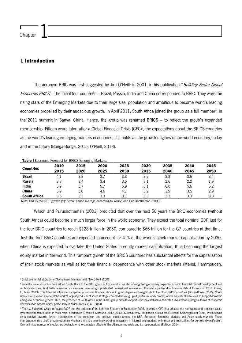
The acronym BRIC was first suggested by Jim O’Neill1 in 2001, in his publication “Building Better Global

Economic BRICs”. The initial four countries – Brazil, Russia, India and China corresponded to BRIC. They were the

rising stars of the Emerging Markets due to their large size, population and ambitious to become world’s leading

economies propelled by their audacious growth. In April 2011, South Africa joined the group as a full member2, in

the 2011 summit in Sanya, China. Hence, the group was renamed BRICS – to reflect the group’s expanded

membership. Fifteen years later, after a Global Financial Crisis (GFC)3, the expectations about the BRICS countries

as the world’s leading emerging markets economies, still holds as the growth engines of the world economy, today

and in the future (Bonga-Bonga, 2015; O’Neill, 2013).

Table I Economic Forecast for BRICS Emerging Markets.

Countries 2010 2015 2020 2025 2030 2035 2040 2045

2015 2020 2025 2030 2035 2040 2045 2050 Brazil 4.1 3.8 3.7 3.8 3.9 3.8 3.6 3.4

Russia 3.8 3.4 3.4 3.5 3.1 2.6 2.2 1.9

India 5.9 5.7 5.7 5.9 6.1 6.0 5.6 5.2

China 5.9 5.0 4.6 4.1 3.9 3.9 3.5 2.9

South Africa 3.6 3.3 3.3 3.1 3.3 3.3 3.3 3.3

Note: BRICS real GDP growth (%): 5-year period average according to Wilson and Purushothaman (2003).

Wilson and Purushothaman (2003) predicted that over the next 50 years the BRIC economies (without

South Africa) could become a much larger force in the world economy. They expect the total nominal GDP just for

the four BRIC countries to reach $128 trillion in 2050, compared to $66 trillion for the G7 countries at that time.

Just the four BRIC countries are expected to account for 41% of the world's stock market capitalization by 2030,

when China is expected to overtake the United States in equity market capitalization, thus becoming the largest

equity market in the world. This rampant growth of the BRICS countries has substantial effects for the capitalization

of their stock markets as well as for their financial dependence with other stock markets (Mensi, Hammoudeh,

1 Chief economist at Goldman Sachs Asset Management. See O’Neill (2001).

2 Recently, several studies have added South Africa to the BRIC group as this country has also a fast-growing economy, experiences rapid financial market development and

sophistication, and is globally recognized as a source possessing sophisticated professional services and financial expertise (Liu, Hammoudeh, & Thompson, 2013; Zhang,

Li, & Yu, 2013). This financial influence is capable to transmit financial shocks in great degree and magnitude to the other BRICS countries (Bonga-Bonga, 2015). South

Africa is also known as one of the world's largest producer of some strategic commodities (e.g., gold, platinum, and chrome) which are critical resources to support domestic

and global economic growth. Thus, the presence of South Africa in the BRICS group provides opportunities to establish a dedicated investment strategy in terms of economic

diversification opportunities, particularly in Africa (Mensi et al., 2014). 3 The US Subprime Crisis in August 2007 and the collapse of the Lehman Brothers in September 2008, sparked a GFC that affected the real sector and caused a rapid,

synchronized deterioration in most major economies (Gentile & Giordano, 2012, 2013). Subsequently, the effects caused the Eurozone Sovereign Debt Crisis, which served

as a catalyst towards further investigation of the contagion and spillover effects among the USA, Eurozone, Emerging Markets and Asian stock markets. These

interdependencies could provide evidence whether there is a seemingly growing integration in international markets with important implications for portfolio diversification.

Only a limited number of studies are available on the contagion effects of the US subprime crisis and its repercussions (Bekiros, 2014).

Chapter 1

2

Reboredo, & Nguyen, 2014; Visalakshmi & Lakshmi, 2016). BRICS’s economies have matured hastily and are

becoming increasingly more integrated with the most developed economies in terms of trade and investment4.

In the past three decades, various countries have been hit by severe financial crises: the Mexican “Tequila

Crisis” in 1994, the East Asian Crisis in 1997, the Russian Crisis in 1998, the Argentinean Crisis in 2002, the

United States of America (USA) Subprime in 2007 and the Lehman Brothers Bankruptcy Crisis (LBBC) in 2008

and, more recently, the European Sovereign Debt Crisis (ESDC) in 2010/2011. All these financial crises started in

a specific country and region in the globe and, subsequently, their effects spread to other countries and regions.

Such transmission of shocks is dubbed contagion (Bonga-Bonga, 2015). Notwithstanding, the contagion term is

not consensual, this research follows the largest body of the empirical literature based on the Forbes and

Rigobon (2002) designation, where contagion is defined as a significant increase of cross-market linkages after a

shock to one country or a group of countries. This contagion effect undermines the purpose of the portfolio

diversification, revealing the situation where markets that were assumed to be weakly associated before a shock

are subsequently found to be strongly associated in such a way that diversification across markets fails to shield

the investors from the unsystematic risk (Gentile & Giordano, 2012, 2013). This definition indicates that, if two

markets present a high degree of co-movement during periods of stability and continue to be highly correlated after

a shock to one market, this indicate interdependence5 rather than contagion.

A comprehensive understanding of the financial market contagion is extremely important to address how

its mechanisms work, to understand and assess its importance and take efficient policy measures. Regarding to

these matters, there are policy implications associated with fundamentals-driven and contagion-driven movements,

two broad concepts defined in the literature (Claessens, Dornbusch, & Park, 2001; Dornbusch, Park, & Claessens,

2000; Forbes & Rigobon, 2001; Gentile & Giordano, 2012, 2013; Masson, 1998). In the first one, measures must

be taken by the policymakers to improve fundamentals. In the second one, if markets have fallen due to contagion,

then the priority should be to improve market sentiments with credible policy actions. Contagion entails an

intensification or change in the transmission of shocks among markets and it requires a structural break, leading

to the identification of tranquil and turbulent periods6. Therefore, the transmission mechanisms during a crisis are

forcibly different from those in a stable period (Gentile & Giordano, 2012).

4 The BRICS together constitute more than a quarter of the world's land area, more than 40% of the world's population and about 15% of global GDP (see Appendix I and II).

The growth potentials in those culturally and geographically disparate countries are based on diverse attributes. Brazil is a resource-rich country, with resources such as

coffee, soybean, sugar cane, iron ore and crude oil. Russia is well known for its massive deposits of oil, natural gas and minerals. India has a rising manufacturing base and

is a strong service provider. China has a highly skilled workforce at low wage cost and it is considered to be the factory of the world. South Africa, the smallest of the five

BRICS countries by land mass and world GDP contribution, is the world’s largest producer of platinum and chromium, and holds the world’s largest known reserves of manganese, platinum group metals, chromium, vanadium and aluminum-silicates (New Delhi, 2012). 5 When co-movements do not increase significantly after a shock, then any continued high level of market correlation indicates strong connections among the countries that

exist worldwide (Gentile & Giordano, 2012). 6 Contagion occurs when there is a significant increase in cross-market co-movements after a shock to one country or a group of countries beyond what would be justified

by fundamentals (Dornbusch et al., 2000). This definition of contagion is not possible to explain just looking for the fundamentals (such as trade or macroeconomic policy

between countries). On the contrary, the presence of contagion assumes that the transmission of shocks is made possible through the Investor’s anticipation, which can

cause contagion due to a shift in the investor-behavior (Gentile & Giordano, 2012, p. 15), changing the flow of international portfolio investments (fight-to-quality phenomenon)

in such a manner that it cannot be explained by economic fundamentals. For example, a crisis in one emerging market country can trigger investors to withdraw funds from

many emerging markets without considering the fundamental economic differences between them (Bonga-Bonga, 2015).

3

This research enriches the literature by focusing the study on the great importance that the effects of

contagion in the financial crises across BRICS countries can reveal based on the magnitude of the interaction

among them and what they represent globally. The focus of this research is pointed towards the LBBC and the

ESDC in order to identify if there was contagion transmission to the BRICS countries and the implications of this

phenomenon due to the great impact that both crises had in the behavior of the investors, which brought massive

inflows of foreign direct investment (FDI)7 to the BRICS countries, trying to hedge their investments (Nistor, 2015).

To achieve this goal, we implemented a three-step methodology that capture the different patterns of

contagion transmission across BRICS countries stock markets, following Baig and Goldfajn (1999), Beirne and

Gieck (2012), Gentile and Giordano (2012, 2013), Fourie and Botha (2015) and Boubaker, Jouini, and

Lahiani (2016). The Johansen cointegration test to detect the cross-market connections in the long-run, allowing

the identification of signs of contagion and the detection of the so called “contagion Windows” by looking direct in

the data without any kind of previous assumptions; the Granger causality/Vector error correction model (VECM),

which captures new significant short connections among the BRICS countries after a financial shock, allowing also

the identification of which country propagates the impulses of contagion (leading countries) and which country is

the target of contagion (follower countries); the last step is dedicated to the rate of involvement indicator, which

identifies the most vulnerable countries, measuring how much of the domestic risk is explained by innovations in

other BRICS countries.

Our results clearly reveal an increase in the long-run connections among BRICS stock markets jointly with

changes in the causality patterns, which have changed in the turbulent periods compared to the tranquil periods.

The evidence suggests that contagion effects strongly influenced the BRICS stock markets over both crises. These

results also reveal that BRICS countries were not able to provide portfolio diversification, indicating that both crises

affected their stock markets, revealing different degrees of vulnerabilities among them.

This empirical research is organized as follows. Section 2 contains a literature review, Section 3 describes

the data and the econometric methodology, which is followed by Section 4, the core section, which presents the

empirical results. Section 5 concludes.

Keywords: Contagion Effect, BRICS Stock Markets, VAR Models, Financial Crises.

7 See Appendix III.

4

2 Literature Review

2.1 Contagion Phenomenon: Definition, Theories, Transmission and Measurement

“(…) countries have become so interdependent in both good and bad times that contagion is extremely difficult to stop. Many measures aimed at minimizing contagion provide only a temporary reprieve and can aggravate contagion risks through other channels.”

(Forbes, 2012, p. 1)

The different definitions of contagion, how it is measured, what causes contagion, how it is transmitted and

why, is extremely important to understand so as to evaluate this phenomenon correctly and develop policy

responses efficiently. Blaming financial crisis on contagion remains an elusive concern, highly contagious among

politicians and economists. Without a clear understanding of financial contagion and the mechanisms through

which it works, we can neither assess the problem nor design appropriate policy measures to control

for it (Moser, 2003). Such understanding is needed to identify the economic implications both for implementing

policies and for investors, who need to understand the nature of changes in stock markets to evaluate the potential

benefits of international portfolio diversification and the analytical assessment of risks.

Despite the significant theoretical and empirical interest of financial contagion, there is still no consensus

about whether cross-county propagation of shocks through fundamentals8 should be considered contagion. Hence,

we need to differentiate between pure contagion9 and shock propagation through fundamentals10. Some have

suggested transmission (Bordo & Murshid, 2000; Lakshmi, Visalakshmi, & Shanmugam, 2015); spillovers (Broto

& Pérez-Quirós, 2015; Dungey & Martin, 2007; Masson, 1998, 1999; Muratori, 2014); interdependence (Forbes

& Rigobon, 2001, 2002, Gentile & Giordano, 2012, 2013) or fundamentals-based contagion11 (Bonga-Bonga, 2015;

8 Financial, real and political links, constitute the fundamentals links of an economy (Gentile & Giordano, 2012; Moser, 2003). The first ones exist when two economies are

connected through the international financial system. Real links are fundamental economic relationships between countries. These links have usually been associated with

international trade, but other types of real links, like foreign direct investment across countries, may also be present. Finally, political links are the political relationships

between countries. Although this link is much less stressed in the literature, when a group of countries share an exchange rate arrangement – a common currency in the

case of the euro area countries – crises tend to be clustered (Gómez-Puig & Sosvilla-Rivero, 2014). 9 Masson (1998) defines pure contagion as an unanticipated situation. Claessens et al. (2001) and Gentile and Giordano (2012) define pure contagion in the sense of

Masson’s only when the transmission process itself changes when entering crises periods: when a crisis in one country may conceivably trigger a crisis elsewhere for reasons

unexplained by macroeconomic fundamentals – perhaps because it leads to shifts in market sentiment, or changes the interpretation given to existing information, or triggers

herding behavior. 10 The theories based on fundamentals channels are the oldest, and the general idea is that links across countries exist because the countries’ economic fundamentals

affect one another. These theories are usually based on standard transmission mechanisms, such as trade, monetary policy, and common shocks (e.g., oil prices), according

Gentile and Giordano (2012, 2013). 11 Fundamentals-based contagion refers to the transmission of shocks that is due to real and financial linkages or fundamental relationship of any kind, such as trade or

macroeconomic policy, between countries (Bonga-Bonga, 2015; Dornbusch et al., 2000; Forbes & Rigobon, 2001; Masson, 1998).

2 Chapter

5

Kaminsky & Reinhart, 1998). This differentiation is defined by Moser (2003), indicating that shocks propagation

through fundamentals is the result of an optimal response to external shocks, which is not considerate a source of

pure contagion. For instance, a crisis in one country can cause disturbances in the equilibrium of other countries,

causing an adjustment in the financial and real variables to a new equilibrium. In that case, financial market

responses only anticipate and reflect changes in fundamentals, accelerating the adjustment to a new equilibrium,

just transmitting and not causing the changes in the equilibrium. In other words, rather than causing a crisis,

financial markets responses bring the crisis forward, being an example of fundamentals-based contagion rather

than pure contagion (Moser, 2003).

In order to explain whether cross-country propagation of shocks is related or not by the fundamentals,

market imperfections is the path to follow and understand. Having said that, two groups can be used to differentiate

the mechanisms of pure contagion according to Moser (2003):

1. Information Effects – information is costly, imperfections and asymmetries can bring difficulties to assess

fundamentals correctly. This situation can generate uncertainty among market participants, causing a

miscomprehension of the true state of a country’s fundamentals12. A crisis elsewhere might lead them to

reassess the fundamentals of other countries and cause them to sell assets, to call in loans, or to stop lending

to these countries, even if their fundamentals remain objectively unchanged (Gentile & Giordano, 2013;

Moser, 2003; Zouhair, Lanouar, & Ajmi, 2014). Goldstein (1998) affirms that a crisis in one country may serve

as a wake-up call for market participants if it causes them to take a closer look at fundamentals similar to those

in the country affected by the crisis13. Contagion occurs if the market participants find problems or risks that

were not detected before (Gentile & Giordano, 2013).

2. Domino Effects – this group explains that a crisis in one country spreads to others as a result of the financial

connections, direct or indirectly, in three possible different ways: by counterparty defaults; portfolio rebalancing

related to liquidity constrains and portfolio rebalancing related to capital constrains. For more detail see (e.g.,

Gentile & Giordano, 2013, p. 202; Moser, 2003).

2.1.1 What is Financial Contagion?

Contagion phenomenon generally is used to describe the spread of market disturbances from one country

to another14. In its broadest sense, therefore, financial contagion is related with the propagation of adverse shocks

that have the potential to trigger financial crises. The core of the matter is to identify potential propagation

mechanisms and define those that represent contagion (Moser, 2003). In spite of the greatest relevance of the

12 Investors do not know enough about the countries in which they invest and therefore try to infer future price changes based on how the rest of the market is reacting. The

relatively uninformed investors follow the supposedly informed investors, and all the market moves jointly (Gómez-Puig & Sosvilla-Rivero, 2014). For example, a crisis in one

emerging market country can trigger investors to withdraw funds from many emerging markets without taking into account the fundamental economic differences between

them (Bonga-Bonga, 2015; Gentile & Giordano, 2012, 2013). 13 The literature offers a few reasons indicating why crisis elsewhere could lead to a revaluation of the fundamentals. For instance, the signal extraction failures, wake-up

call, expectations interactions, moral hazard plays and membership contagion (Moser, 2003). 14 The process can be observed through co-movements in exchange rates, stock prices, sovereign spreads and capital flows (Gentile & Giordano, 2012).

6

contagion phenomenon, there is still no consensus on either the definition or the transmission channels of financial

contagion. As a first step, it is helpful to understand what contagion does not mean and what it does mean.

The World Bank (2016) distinguishes three definitions of financial contagion: broad, restrictive and very

restrictive.

The broad definition: it is vague and generalist, this definition was used in the earlies stages of the research

on contagion phenomenon. Under this approach, contagion is the cross-country transmission of shocks or the

general cross-country spillover effects during the crisis (Gentile & Giordano, 2012, 2013). Furthermore, this

definition also claims that contagion can take place during both “good” times and “bad” times, indicating that

contagion does not need to be related to crises. However, contagion has been emphasized during crisis periods.

Using the broad definition is difficult, since it does not provide a framework to work with, no triggering event is

involved and, a priori, no underlying relationships are supposed. Within this definition, recent works about spillovers

propagation can be seen in the research of Diebold and Yilmaz (2008). Corsetti, Pericoli, and Sbracia (2001) specify

that contagion occurs when a country-specific shock becomes “regional” or “global”, which fits also the broad

definition of contagion.

The restrictive definition: it is suitable in more recent literature, where contagion is the transmission of

shocks from one country to others or the cross-country correlation, beyond what would be explained by

fundamentals or common shocks15. This definition is usually referred to as excess co-movement16, commonly

explained by herding behavior. The research of Eichengreen, Rose, and Wyplosz (1996) and Bekaert, Harvey, and

Ng (2005) can be fit into this definition. For instance, Masson (1998, 1999) defines contagion as a transmission

of crises that cannot be identified with observed changes in macroeconomic fundamentals. Therefore, the restrictive

definition of contagion does not need any type of link among countries, implying that contagion should be explained

by causes beyond any fundamentals links, namely, herd behavior, financial panics, or switches of expectations

across instantaneous equilibria (Corsetti et al., 2001).

The very restrictive definition: it implies an increase in the linkages after a crisis, when cross-country

correlations increase during “crisis times” relative to correlations during “tranquil times”, therefore, this can only

be due to factors unrelated to fundamentals, since they cannot change in a short period of time (Gentile &

Giordano, 2012, 2013). In fact, Dornbusch et al. (2000) and Forbes and Rigobon (2002) argue that contagion is a

significant increase in cross-market co-movements after a (negative) shock to one country (or group of countries).

This definition is known sometimes as “shift-contagion17”. Forbes and Rigobon (2001) reinforce that this notion of

contagion excludes a constant high degree of co-movement in a crisis period, otherwise markets would be just

15 Fundamentals causes of contagion include macroeconomic shocks that have repercussions on an international scale and local shocks transmitted through trade links,

competitive devaluations, and financial links (Gentile & Giordano, 2012, 2013). 16 That means a correlation that remains even after controlling for fundamentals and common shocks. Herding behavior is usually said to be responsible for co-movement

beyond that explained by fundamentals linkages (Gentile & Giordano, 2012). 17 Our definition of “shift contagion “ following Gentile and Giordano (2012), relies on a significant increase in cross-market co-movements after a shock, which is not related

with fundamentals linkages (such as financial, real or political). The only transmission channel that could explain contagion is the behavioral one.

7

interdependent18. There is contagion only if cross-market co-movements increase significantly after the shock19. Any

continued high level of market correlation suggests strong linkages between the two economies that exist in all

states of the world. This definition implies the presence of a tranquil, pre-crisis period, requiring that contagion

effects are to be differentiate from “normal” transmission of shocks across countries, usually defined as

interdependencies (Bae, Karolyi, & Stulz, 2003; Corsetti, Pericoli, & Sbracia, 2005; Forbes & Rigobon, 2002;

Gentile & Giordano, 2012, 2013; Gómez-Puig & Sosvilla-Rivero, 2014). In addition, Edwards (2000) asserts that

contagion reflect a situation in which the effect of an external shock is larger than what was expected by experts

and analysts, implying that contagion has to be differentiated from the “normal” transmission of shocks across

countries.

Currently this very restrictive definition reveals two major advantages: firstly, it provides a straightforward

framework for testing whether contagion occurs or not by comparing co-movements between two markets (such as

cross-market correlations coefficients) during a relatively stable period with co-movements immediately after a

shock or crisis, which does not require a specification of a structural representation for stock returns. Secondly, it

allows distinguishing between permanent and temporal mechanisms of crises transmission. Identifying if the

propagation of a crisis is due to permanent or temporal mechanisms has important implications for designing

public policy responses (Bejarano-Bejarano, Gomez-Gonzalez, Melo-Velandia, & Torres-Gorron, 2015). There are

several researches based on this definition20.

This empirical research uses the very restrictive definition of contagion, because it provides an alternative

explanation for transmission of crisis, namely interdependence, allowing one to answer the questions: Is there

contagion or interdependence? Do the periods of highly correlated market movements provide evidence of

contagion? Does the cross-market relationship change during periods of crisis? Our main goal is to try to answer

these questions in the context of both crises (LBBC and ESDC) from the perspective of the BRICS countries stock

markets.

2.1.2 Causes and Transmission of Contagion

The literature divides the concept of contagion into two broad categories (Bonga-Bonga, 2015; Dornbusch

et al., 2000; Forbes & Rigobon, 2001; Masson, 1998; Pritsker, 2000), namely, fundamentals-based21 and investor-

behavior contagions. The first category emphasizes spillovers that result from the normal interdependence among

18 Regarding the extreme definition of contagion phenomenon, for instance, the research of Bae, Karolyi, and Stulz (2000, 2003) consider extreme return shocks across

countries as evidence for contagion. 19 A contagious event cannot occur in the absence of a shock, indicating that a large shock should occur (Caporin et al., 2013; Constâncio, 2012).

20 See, for example, Forbes and Rigobon (2002), Pericoli and Sbracia (2003), Samarakoon (2011), Constâncio (2012), Kalbaska and Gątkowski (2012), Gentile and

Giordano (2012, 2013), Bejarano-Bejarano et al. (2015), and Luchtenberg and Vu (2015). 21 Fundamentals-based contagion is caused by “monsoonal effects” and “linkages”. Monsoonal effects – are random aggregate shocks that hit a number of countries in a

similar way (such as a major economic shift in industrial countries, a significant change in oil prices or changes in US interest rates) that may adversely affect the economic

fundamentals of several economies simultaneously and, therefore, may cause a crisis (Eichengreen et al., 1996; Masson, 1998). Linkages – are normal interdependencies,

such as those produced by trade and financial relations between countries and which can easily become a carrier of crisis (Kaminsky & Reinhart, 2000; Masson, 1998).

8

market economies, referring to the transmission of shocks that is due to real and financial linkages or fundamentals

relationship of any kind, such as trade or macroeconomic policy, between countries. These forms of co-movements

would not indicate contagion, according to the restrictive and very restrictive definition of contagion, which is

adopted in this research. According to Gentile and Giordano (2012), fundamentals linkages cannot change suddenly

in a few months after a shock has occurred. Hence, that is considered interdependence.

The second category involves a financial crisis that is not linked to observed changes in macroeconomics

or other fundamentals but is solely the result of a change in investor behavior which alters the flow of international

portfolio investments in such a manner that it cannot be explained by economic fundamentals. Under this definition,

contagion arises when a co-movement occurs, even when there are no global shocks and interdependence and

fundamentals are not factors. For example, a crisis in one emerging market country can trigger investors to withdraw

funds from many emerging markets without taking into account the fundamental economic differences between

them22 (Bonga-Bonga, 2015). If the transmission force is based on the irrational behavior of the market agents,

known as “irrational” phenomena23, then even countries with good fundamentals can be seriously affected, in this

case we have contagion. On the other hand, if the crisis is transmitted through stable fundamentals linkages, then

only countries with fragile economic fundamentals will be affected while those with good fundamentals can be

protected. In that case, we have only interdependence (Gentile & Giordano, 2012).

Table II Fundamentals Causes of Contagion24.

Fundamentals-based Investor's behavior 1) Common shocks 1) Liquidity problems

2) Trade links and competitive devaluations 2) Information asymmetries and costs

3) Real and financial links 3) Multiple equilibriums

4) Macroeconomic policies 4) Changes in the rules of the game

The degree of financial market integration determines how immune to contagion countries are25. The spread

of a crisis depends on the degree of financial market integration26. The higher the degree of integration, the more

extensive could be the contagious effects of a common shock or a real shock to another country. Conversely,

countries that are not financially integrated, because of capital controls or lack of access to international financing,

22 This event is known as “Fight-to-quality phenomenon” and refers to a sudden shift in investment behaviors in a period of financial turmoil where investors try to sell assets

perceived as risky and instead purchase safe assets. An important feature of flight-to-quality is an insufficient risk taking behavior by investors. Though excessive risk taking

can be a source of financial crisis, insufficient risk taking can severely dislocate credit and other financial markets during the financial crisis. These shifts in portfolio

investments result in further negative shocks to the financial sector. In accordance to this phenomenon demand for 10-year US Treasuries and gold increased during the

recent financial turmoil (Kazi & Wagan, 2014). 23 This can occur in the form of speculative attacks, financial panics, herd behavior, loss of confidence, and increased risk aversion (Gentile & Giordano, 2012, 2013).

24 Macroeconomics causes. See for example, Dornbusch et al. (2000) and Claessens et al. (2001).

25 For example, Chinese and Indian economies are relatively closed and feature state-controlled capital markets, meaning that their development strategy is based on

domestic industrialization catering to export markets. However, the Brazilian and Russian economies are based on natural resources and are much more open and currently

subject to relatively less state control (Zouhair et al., 2014). South Africa is also based on natural resources and is much more open and currently subject to relatively less

state control. In fact, is the most liberalized financial market in the BRICS countries (Bonga-Bonga, 2015). 26 Despite its many advantages, in the short-term, financial liberalization is often accompanied by a wave of financial crises, many of which have taken a systemic extent and

hit, in particular, the newly liberalized economies (Ben Rejeb & Boughrara, 2015). This Integration increased interdependence causes extreme negative events in one country

to quickly affect others. These extreme negative events, and their joint coincidence across countries, have increased over time, creating substantial challenges for countries

affected by contagion (Forbes, 2012).

9

are by definition immune to contagion (Dornbusch et al., 2000). This is correct because of our very restrictive

definition, however, it might not be true for other definitions of contagion.

The initial literature has generally been divided as to whether transmission through real or financial channels

constitutes contagion. Forbes and Rigobon (2001, 2002), Gentile and Giordano (2012) argue that the theoretical

literature of contagion could be split into two groups: crisis-contingent and non-crisis-contingent theories.

Table III Possible Explanation for Contagion.

Crisis-Contingent Theories Non-Crisis-Contingent Theories

1) Multiple equilibria27 1) Trade

2) Endogenous liquidity shocks 2) Policy coordination

3) Political contagion 3) Country reevaluation

4) Random global monetary shocks 4) Random real global shocks

The first one is related to the financial linkages, explaining why transmission mechanisms change during a

crisis and therefore why a shock leads to an increase in the cross-market linkages. On the other hand, the second

one is related to the real linkages, if transmission mechanisms are the same during a crisis as during more stable

periods, and therefore cross-market linkages do not change (increase) after a shock. Theories belonging to the

second group may be interpreted as interdependence rather than contagion28.

2.1.3 Contagion: Testing and Measurement

Gentile and Giordano (2012, 2013) describe contagion as the amount of co-movement among asset prices

which exceeds what is explained by fundamentals, since fundamentals cannot change in a few months. They argue

that a degree of extreme connection or asymmetry that goes beyond interdependencies must be present in order

for contagion to be present.

Research on contagion range from testing conditional correlation to contagion of bond spreads, sovereign

ratings, credit default swaps (CDS) spreads, stock market returns, differences in interest rates, common trends

and cycles, monetary policy and currency market (Bianconi, Yoshino, & Machado de Sousa, 2013; Caporin,

Pelizzon, Ravazzolo, & Rigobon, 2013; Fourie & Botha, 2015; Gentile & Giordano, 2012, 2013, Gómez-Puig &

Sosvilla-Rivero, 2014, 2011; Matos, Oquendo, & Trompieri, 2015)29. For instance, Forbes and Rigobon (2001)

discriminated empirically between contagion and interdependencies by testing whether or not cross-market

correlation increases statistically significantly in crisis periods. If that is the case, crisis-contingent theories have a

point, otherwise, interdependencies are responsible for the spread of crisis. Furthermore, Forbes and

27 Multiple equilibria, occurs when a crisis in one country is used as a “sunspot” variable for other countries (Forbes & Rigobon, 2001). For example, Masson (1998) and

Gentile and Giordano (2013) show how a crisis in one country could coordinate investors’ expectations, shifting them from a good to a bad equilibrium for another economy

and thereby cause a crash in the second economy. 28 For more detail, see, for example, Forbes and Rigobon (2002). As said before, the transmission of shocks through the first two linkages (financial and real) is considered

as interdependence or spillovers (Gentile & Giordano, 2012). 29 And others (Aloui, Aïssa, & Nguyen, 2011; Andenmatten & Brill, 2011; Ang & Chen, 2002; Baur, 2012; Beirne & Gieck, 2012; Bonga-Bonga, 2015; Boubaker et al.,

2016; Campbell, Forbes, Koedijk, & Kofman, 2006; Constâncio, 2012; Favero & Giavazzi, 2000; Forbes, 2012; Forbes & Rigobon, 2001, 2002; Khalid & Kawai, 2003;

Pontines & Siregar, 2007; Saghaian, 2010; Suleimann, 2003; Zouhair et al., 2014).

10

Rigobon (2002) argue that simple correlation are biased due to the presence of heteroskedasticity, endogeneity,

and omitted variables30. After correcting for these statistical problems for the case of the 1994 Mexican crisis, the

1997 Asian Crisis, and the 1987 USA stock market crash, they found only interdependence, no pure contagion31.

Andenmatten and Brill (2011), following Forbes and Rigobon (2002) methodology, also performed a

bivariate test for contagion to examine whether the co-movement of sovereign CDS premium increased significantly

after the beginning of Greek debt crisis in October 2009. The findings revealed that in European countries, both

contagion and interdependence occurred. In addition, Baig and Goldfajn (1999) in the context of the Asian crisis,

using the same methodology, performed a cross-market correlation for exchange rates, stock returns, interest rates,

and sovereign bond spreads. The findings for sovereign spreads highlighted strong evidence of contagion and high

correlation among exchange rate, stock returns and interest rates co-movements. They conclude that spreads

directly reflecting the risk perception of financial markets, indicating that pure contagion may be the result of the

behavior of investors or other financial agents (Claessens et al., 2001).

Extending the study related to the 1997 Asian crisis, Khalid and Kawai (2003) using the Granger causality

and Impulse responses methodology for nine East Asian countries, tested for contagion based on three main

financial markets indicators: foreign exchange rates, stock market prices and interest rates. The empirical evidence,

however, did not find strong support for contagion.

Bonga-Bonga (2015) provides evidence of contagion phenomenon by analyzing financial contagion between

South Africa and its BRICS equity market from December 1996 to May 2012, the initial period corresponds with

the liberalization of a number of BRICS equity markets. By applying a conditional correlation framework, they find

evidence of cross-transmission and dependence between South Africa and Brazil. Furthermore, the research also

ascertained that South Africa is more affected by crises originating from China, India and Russia than these

countries are by crises from South Africa. Furthermore, Matos et al. (2015) performed a test to identify common

trends and cycles between BRIC’s stock markets, providing evidence of contagion effect, with Brazil and China

financial markets playing a leading role in the transmission of contagion. They conclude that worldwide investors

should consider reactions in Chinese and Brazilian markets during a crisis as a predictor of other BRIC reactions

through the contagion channel32, while policy makers should remain attentive to the level of contagion observed,

given its relevance when evaluating the effectiveness of interventions and financial assistance packages after crisis.

A wide range of empirical techniques has been used to quantify contagion in the literature. For instance,

Forbes (2012) refers tools to measure contagion range from cross-market correlations analysis (Forbes &

Rigobon, 2001, 2002) to probability analysis (Constâncio, 2012; Eichengreen et al., 1996; Gómez-Puig &

30 During times of increased volatility (i.e., in time of crisis) estimates of correlation are biased upward. If co-movement tests are not adjusted for that bias, contagion is too

easily detected. 31 After they have adjusted the correlation coefficient, taking in account the changes in volatility. Notwithstanding, Corsetti, Pericoli, and Sbracia (2005) have contested this

methodology, indicating that this conclusion cannot be empirically generalized. 32 Trade, banks/lending institutions, portfolio investors and wake-up calls/fundamentals reassessment (Forbes, 2012).

11

Sosvilla-Rivero, 2014, 2011) to latent factor/GARCH models (Bekaert, Ehrmann, Fratzscher, & Mehl, 2011; Bekaert

et al., 2005; Dungey & Yalama, 2010) to extreme values/co-exceedance/jump (Bae et al., 2003; Berger &

Pukthuanthong, 2012; Boyer, 2006; Forbes, 2012) and VAR models33 (Beirne & Gieck, 2012; Favero & Giavazzi,

2002; Fourie & Botha, 2015; Gentile & Giordano, 2012, 2013; Matos et al., 2015; Syriopoulos et al., 2015).

More related to our approach, Boubaker et al. (2016) use VAR-VECM to measure contagion between US

stock market and developed and emerging stock markets during the Subprime crisis in September 2008. They

provided significant evidence of contagion effects between the US stock market and the developed and emerging

equity markets after the global financial crisis. Beirne and Gieck (2012) use a global VAR to measure

interdependence and contagion across bonds, stocks and currencies for over 60 economies during periods of crisis.

Their analysis reveals that shocks to equity markets typically originate in the US and that bond market shocks tend

to originate in the Eurozone. Gentile and Giordano (2012, 2013) use cointegration and VECM/Granger causality

tests to measure the existence and direction of contagion in European countries during the LBBC and ESDC,

pointing out the occurrence of contagion phenomenon in both crises. Fourie and Botha (2015) using the same

methodology provided by Gentile and Giordano (2012, 2013), but for sovereign ratings, proved contagion in

European countries, during the two recent windows of crises: Lehman Crisis and European Union Sovereign Debt

Crisis.

Andenmatten and Brill (2011) perform a bivariate test for contagion that is based on an approach proposed

by Forbes and Rigobon (2002) to examine whether the co-movement of sovereign CDS premium increased

significantly in emerging and industrialized countries during the Greek debt crisis of 2009. They conclude that

contagion and interdependence occurred. Saghaian (2010) uses Granger causality to create contemporaneous

contagion links between agriculture and energy markets within the commodity sector. Suleimann (2003) uses VAR

to measure contagion in technology stock prices between Europe and the United States. Pontines and

Siregar (2007) use Markov Switching and VAR to measure contagion in East Asian markets using stock exchange

returns during periods of turbulence. Favero and Giavazzi (2000) use VAR to test contagion using money market

spreads across European Monetary Union countries. Baig and Goldfajn (1999) use dummy variables in VAR and

correlation models to prove contagion during the East Asian crisis.

33 These models are closely related to the use of correlation coefficients to analyze contagion. Generally, they predict stock market returns or yield spreads while controlling

for global factors and country-specific factors, as well as for the persistence of these factors through error-correction techniques. Contagion is then measured with an impulse-

response function predicting the impact of an unanticipated shock to one country on others. These tests are less conservative than those based on correlation coefficients

as they generally do not adjust for the heteroskedasticity in returns (and attempts to make this adjustment generate fragile results). Not surprisingly, papers using VARs

generally find more evidence of contagion (Forbes, 2012).

12

3 Data & Methodology

3.1 Data

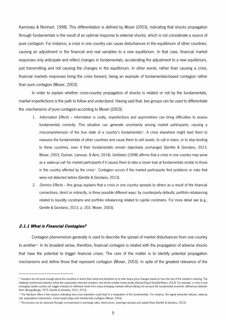
Our main objective is to test for contagion during the last two international financial crises34, using an

important financial market indicator: The Stock Market Index (SMI). Further on, we apply a tree-step econometric

analysis35 to test for contagion that will be discussed in detail later. We will analyze the different connections and

co-movement between countries to identify any cross-market or cross-country connections that can explain and

assess contagion phenomena in the BRICS stock markets36.

Morgan Stanley Capital International (MSCI)37 for large-caps is the main source used for stock price indices.

The sample consists of five countries from the Emerging Markets known as BRICS: (Brazil (BRA), Russia (RUS),

India (IND), China (CHI) and South Africa (SAF)) and one developed country, the United States (USA), using daily

stock indices closing prices for each country. The daily frequency sample was considered, because interdependence

phenomena can explode in a few days. So if we had considered weekly or monthly data (lower frequency data), we

could have lost the measurement of interactions (innovations), which may last only a few days (Gentile & Giordano,

2012, 2013; Jin & An, 2016; Voronkova, 2004).

Table 1 Variables Explanation.

Variables Explanation Type

BRA Log-level value of MSCI Brazil (large-caps) Stock Price Index Exogenous/Endogenous

RUS Log-level value of MSCI Russia (large-caps) Stock Price Index Exogenous/Endogenous

IND Log-level value of MSCI India (large-caps) Stock Price Index Exogenous/Endogenous

CHI Log-level value of MSCI China (large-caps) Stock Price Index Exogenous/Endogenous

SAF Log-level value of MSCI South Africa (large-caps) Stock Price Index Exogenous/Endogenous

USA Log-level value of MSCI United States (large-caps) Stock Price Index Exogenous

Note: Regarding to national holidays, the index level was assumed to stay the same as that on the previous trading day. The USA variable is implicitly

imputed in the data, because as it is stated in the literature that linkage patterns may be distorted when the influence of the US market is not taken into

consideration38.

The daily stock indices (in log-level) were presented also through graphical representation over the period

of the study (see Figure 1). Visually, all indices were recovering jointly from 2003 until the beginning of the 2008

34 The recent Lehman Brother bankruptcy Crisis (LBBC) and European Sovereign Debt Crisis (ESDC).

35 First: A bivariate dynamic cointegration analysis; Second: Granger causality test and VECM/Gonzalo-Granger statistic; Third: we apply the Variance decomposition method

following Baig and Goldfajn (1999), Beirne and Gieck (2012), Gentile and Giordano (2012, 2013), Fourie and Botha (2015) and Boubaker et al. (2016). 36 The methodology that will be implemented is based on the definition of contagion as a significant increase of the total number of cross-market connections around the

two crises following the definition of contagion suggested by Forbes and Rigobon (2002), Gentile and Giordano (2012, 2013) and World Bank (2016). 37 For more detail see www.msci.com.

38 For more details, see Khalid and Kawai (2003), Yang et al. (2003), Bekaert, Ehrmann, Fratzscher, and Mehl (2011), and Gentile and Giordano (2012, 2013).

Chapter 3

13

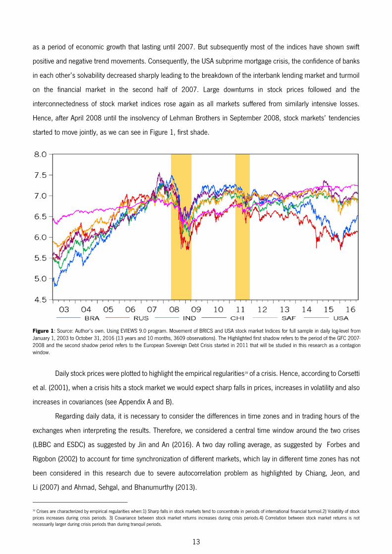
as a period of economic growth that lasting until 2007. But subsequently most of the indices have shown swift

positive and negative trend movements. Consequently, the USA subprime mortgage crisis, the confidence of banks

in each other’s solvability decreased sharply leading to the breakdown of the interbank lending market and turmoil

on the financial market in the second half of 2007. Large downturns in stock prices followed and the

interconnectedness of stock market indices rose again as all markets suffered from similarly intensive losses.

Hence, after April 2008 until the insolvency of Lehman Brothers in September 2008, stock markets’ tendencies

started to move jointly, as we can see in Figure 1, first shade.

Daily stock prices were plotted to highlight the empirical regularities39 of a crisis. Hence, according to Corsetti

et al. (2001), when a crisis hits a stock market we would expect sharp falls in prices, increases in volatility and also

increases in covariances (see Appendix A and B).

Regarding daily data, it is necessary to consider the differences in time zones and in trading hours of the

exchanges when interpreting the results. Therefore, we considered a central time window around the two crises

(LBBC and ESDC) as suggested by Jin and An (2016). A two day rolling average, as suggested by Forbes and

Rigobon (2002) to account for time synchronization of different markets, which lay in different time zones has not

been considered in this research due to severe autocorrelation problem as highlighted by Chiang, Jeon, and

Li (2007) and Ahmad, Sehgal, and Bhanumurthy (2013).

39 Crises are characterized by empirical regularities when:1) Sharp falls in stock markets tend to concentrate in periods of international financial turmoil.2) Volatility of stock

prices increases during crisis periods. 3) Covariance between stock market returns increases during crisis periods.4) Correlation between stock market returns is not

necessarily larger during crisis periods than during tranquil periods.

Figure 1: Source: Author’s own. Using EVIEWS 9.0 program. Movement of BRICS and USA stock market Indices for full sample in daily log-level from

January 1, 2003 to October 31, 2016 (13 years and 10 months, 3609 observations). The Highlighted first shadow refers to the period of the GFC 2007-

2008 and the second shadow period refers to the European Sovereign Debt Crisis started in 2011 that will be studied in this research as a contagion

window.

14

3.1.1 Variable Transformation

We took natural logarithms of our data before proceeding to the analysis process (see table 1). The log form

of stock indices were used in order to reduce the heteroskedasticity present in the data (Singh & Kaur, 2016),

smoothing out the fluctuations (see appendix D and E), to make the data series linear and very helpful for the

purpose of further analysis (Verma & Rani, 2016). Moreover, for evaluating the rate of daily returns needed for

further analysis40, the initially log-level variables were taken and calculated (Ahmad et al., 2013; Malliaris & Urrutia,

1992; Mensah & Alagidede, 2017; Pragidis & Chionis, 2014; Syriopoulos et al., 2015) on the following basis:

� = [l�� � − l�� � − × ] = [l�� ����− × ] (1)

Where, � is the percentage daily returns value at time , � and � − , are the percentage daily returns value at

two successive days: and − , respectively.

After the transformation, the percentage daily stock return variables were defined as: SRBRA, SRRUS,

SRIND, SRCHI, SRSAF and SRUSA (see appendix C).

Daily closing prices of the BRICS stock markets were retrieved from Thomson Reuters Datastream database

and are expressed in US dollars41, and the time range of the time series goes from January 1, 2003 to October 31,

201642. Eviews 9.0 and R programming were used for arranging the data and implementation of econometric

analyses.

3.1.2 Descriptive Statistics

For ascertaining preliminary know-how of behavioral characteristics of the data, Table 2 presents descriptive

statistics of all the return indices.

In Table 2 we present descriptive statistics of BRICS and USA stock market indices from January 1, 2003

to October 31, 2016. As shown, stock returns changes demonstrate a slightly positive mean, which indicate that

stock returns increases have been larger than its decreases in the sample period. On average, the highest returns

are given by SRBRA (0.044%), SRCHI (0.041%) followed by SRIND (0.040%). Regarding to the stock return of SRRUS

and SRBRA present the higher risk and volatility related to the other variables (Std. Dev.: 2.39% and 2.24%,

respectively). Concerning skewness, which is a measure of asymmetry of the distribution of the series around its

mean, has shown that the values are negatively skewed (excluding for SRCHI, which is positively skewed), indicating

that there is a higher probability for investors to get negative rather positive returns from all the other variables.

40 To deal with the unit root that we will see in further analysis.

41 Using US dollars: 1) it is possible to avoid volatility that is induced by monetary phenomena such as inflation rates; 2) Avoid the impact of exchange rates; 3) US dollars

are especially relevant to international investors because of the interpretation problems in using stock indices denominated in the local currency (Bekaert & Harvey, 1995;

Chen et al., 2002; Mollah, Zafirov, & Quoreshi, 2014; Roll, 1992; Singh & Kaur, 2016). 42 Data was set in the begin of 2003 to avoid contamination in the stock market from earlier bond crises in Russia and Latin America (Cronin, Flavin, & Sheenan, 2016, p.

6).

15

Kurtosis measures the peakedness or flatness of the distribution of the series. The sample distributions of SRBRA,

SRRUS, SRIND, SRCHI, SRSAF and SRUSA are skewed left and leptokurtic43. Kurtosis is higher than (� > )44 for

these six variables, confirming significant non-normality (see Appendix E). In addition, the Jarque-Bera (JB) test

(Jarque & Bera, 1980), is a test statistic for testing whether the series is normally distributed or not. JB test statistics

clearly rejects the null hypothesis of normality for all the variables in the study, probability value is very small

(p-value = 0,0000), rejecting the normality at 1% level. The Ljung–Box statistic test (Ljung & Box, 1978), detected

significant autocorrelation in all cases, probability value is also very small (p-value = 0,0000), rejecting the null

hypothesis of no serial correlation, as we can see in Table 2.

Table 2 Descriptive Statistics (log-level)

Variables N Mean Std. Dev. Skewness Kurtosis Jarque-Bera

BRA 3609 6.5376 0.6074 -0.8550 2.9614 439.92*

RUS 3609 6.4310 0.3996 -0.0349 2.3848 57.639*

IND 3609 6.6023 0.4657 -1.1810 3.3801 860.64*

CHI 3609 6.7525 0.4680 -1.0687 2.9950 686.93*

SAF 3609 6.7473 0.3460 -1.1261 3.2410 771.53*

USA 3609 6.7967 0.2485 0.2497 2.3321 104.57*

Descriptive Statistics (percentage stock return)

Variables N Mean (%) Std. Dev. (%) Skewness Kurtosis Jarque-Bera

SRBRA 3609 0.0440 2.2425 -0.2206 10.143 7700.9*

SRRUS 3609 0.0169 2.3788 -0.4298 17.442 31473.*

SRIND 3609 0.0397 1.7098 -0.0369 12.280 12916.*

SRCHI 3609 0.0412 1.7646 0.0239 10.018 7406.6*

SRSAF 3609 0.0288 1.9166 -0.2216 7.2509 2746.8*

SRUSA 3609 0.0233 1.1540 -0.3050 14.994 21689.*

Note: Source: Author’s own based on Eviews 9.0 program. Representation of full sample of log-level and daily stock returns in percentage. (*) probability

value (p-value) significant at 1% level. The Ljung-Box test for SRBRA (62.992*), SRRUS (106.43*), SRIND (85.003*), SRCHI (60.234*), SRSAF (52.641*)

and SRUSA (116.04*), respectively.

3.2 Methodology

3.2.1 Testing for Stationarity

Our financial time series are non-stationarity. The term stationary means that the series should have mean,

variance, and covariance unchanged by the time change (Singh & Kaur, 2016). In order to test the stationarity, the

Augmented Dickey-Fuller (ADF) test (Dickey & Fuller, 1979, 1981) and Phillip-Perron (PP) test (Phillips &

Perron, 1988), were used. A cointegration relationship requires the series to be non-stationary. Hence, it is

necessary to conduct unit root tests45 of all series included in the analysis to establish the order of integration of all

variables. For that purpose, two different specifications of ADF tests and PP tests were applied. The first one includes

43 Financial series are commonly leptokurtic, the kurtosis value is a largely positive. Meaning that, the statistical distribution is clustered, resulting in a higher peak, or higher

kurtosis, than the curvature found in a normal distribution. This high peak and corresponding fat tails mean the distribution is more clustered around the mean than in a

mesokurtic or platykurtic distribution and has a relatively smaller standard deviation. 44 Regarding (� < ), we can see, for example, the log-level variables – BRA, RUS, CHI and USA can be considered as a platykurtic distribution (see appendix D).

45 Variables series that contains unit root is considered to be nonstationary. ( ) denotes integration of order ; ( ) denotes unit root and ( ) denotes stationarity.

16

(2)

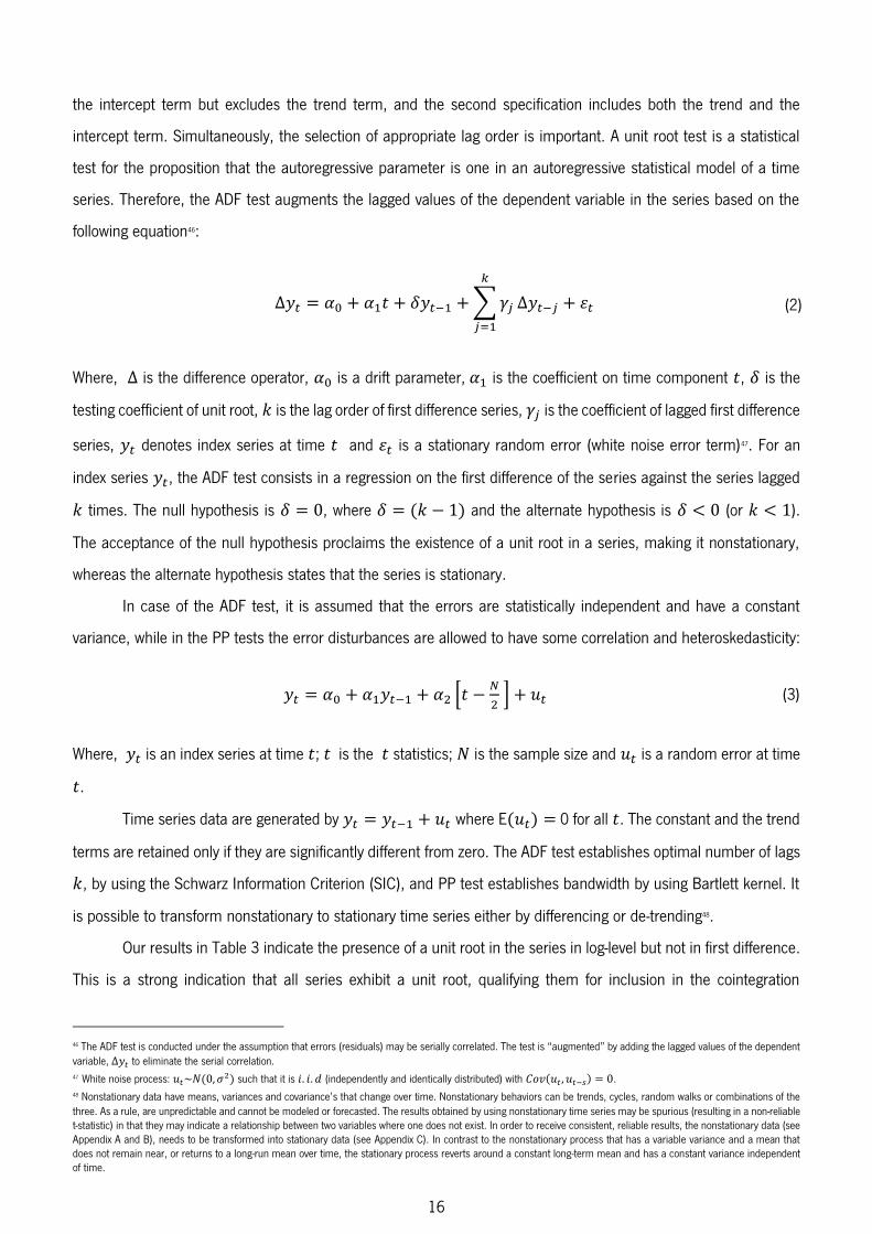
the intercept term but excludes the trend term, and the second specification includes both the trend and the

intercept term. Simultaneously, the selection of appropriate lag order is important. A unit root test is a statistical

test for the proposition that the autoregressive parameter is one in an autoregressive statistical model of a time

series. Therefore, the ADF test augments the lagged values of the dependent variable in the series based on the

following equation46:

∆ = + + − + ∑= ∆ − +

Where, ∆ is the difference operator, is a drift parameter, is the coefficient on time component , is the

testing coefficient of unit root, is the lag order of first difference series, is the coefficient of lagged first difference

series, denotes index series at time and is a stationary random error (white noise error term)47. For an

index series , the ADF test consists in a regression on the first difference of the series against the series lagged

times. The null hypothesis is = , where = − and the alternate hypothesis is < (or < ).

The acceptance of the null hypothesis proclaims the existence of a unit root in a series, making it nonstationary,

whereas the alternate hypothesis states that the series is stationary.

In case of the ADF test, it is assumed that the errors are statistically independent and have a constant

variance, while in the PP tests the error disturbances are allowed to have some correlation and heteroskedasticity:

= + − + [ − ] + (3)

Where, is an index series at time ; is the statistics; � is the sample size and is a random error at time

.

Time series data are generated by = − + where E = 0 for all . The constant and the trend

terms are retained only if they are significantly different from zero. The ADF test establishes optimal number of lags

, by using the Schwarz Information Criterion (SIC), and PP test establishes bandwidth by using Bartlett kernel. It

is possible to transform nonstationary to stationary time series either by differencing or de-trending48.

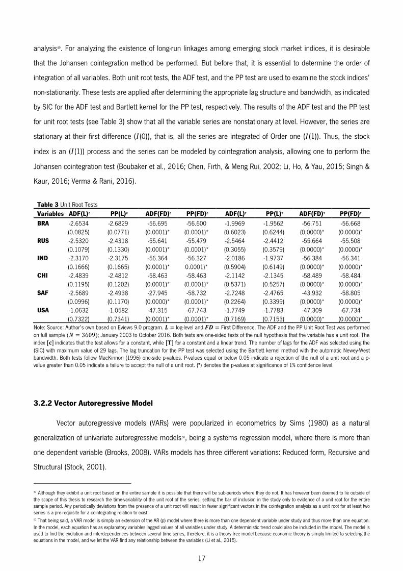
Our results in Table 3 indicate the presence of a unit root in the series in log-level but not in first difference.

This is a strong indication that all series exhibit a unit root, qualifying them for inclusion in the cointegration

46 The ADF test is conducted under the assumption that errors (residuals) may be serially correlated. The test is “augmented” by adding the lagged values of the dependent

variable, ∆ to eliminate the serial correlation.

47 White noise process: ~� ,� such that it is . . (independently and identically distributed) with � , − = . 48 Nonstationary data have means, variances and covariance’s that change over time. Nonstationary behaviors can be trends, cycles, random walks or combinations of the

three. As a rule, are unpredictable and cannot be modeled or forecasted. The results obtained by using nonstationary time series may be spurious (resulting in a non-reliable

t-statistic) in that they may indicate a relationship between two variables where one does not exist. In order to receive consistent, reliable results, the nonstationary data (see

Appendix A and B), needs to be transformed into stationary data (see Appendix C). In contrast to the nonstationary process that has a variable variance and a mean that

does not remain near, or returns to a long-run mean over time, the stationary process reverts around a constant long-term mean and has a constant variance independent

of time.

17

analysis49. For analyzing the existence of long-run linkages among emerging stock market indices, it is desirable

that the Johansen cointegration method be performed. But before that, it is essential to determine the order of

integration of all variables. Both unit root tests, the ADF test, and the PP test are used to examine the stock indices’

non-stationarity. These tests are applied after determining the appropriate lag structure and bandwidth, as indicated

by SIC for the ADF test and Bartlett kernel for the PP test, respectively. The results of the ADF test and the PP test

for unit root tests (see Table 3) show that all the variable series are nonstationary at level. However, the series are

stationary at their first difference ( (0)), that is, all the series are integrated of Order one ( (1)). Thus, the stock

index is an ( (1)) process and the series can be modeled by cointegration analysis, allowing one to perform the

Johansen cointegration test (Boubaker et al., 2016; Chen, Firth, & Meng Rui, 2002; Li, Ho, & Yau, 2015; Singh &

Kaur, 2016; Verma & Rani, 2016).

Table 3 Unit Root Tests

Variables ADF(L)C PP(L)C ADF(FD)C PP(FD)C ADF(L)T PP(L)T ADF(FD)T PP(FD)T

BRA -2.6534 -2.6829 -56.695 -56.600 -1.9969 -1.9562 -56.751 -56.668

(0.0825) (0.0771) (0.0001)* (0.0001)* (0.6023) (0.6244) (0.0000)* (0.0000)*

RUS -2.5320 -2.4318 -55.641 -55.479 -2.5464 -2.4412 -55.664 -55.508

(0.1079) (0.1330) (0.0001)* (0.0001)* (0.3055) (0.3579) (0.0000)* (0.0000)*

IND -2.3170 -2.3175 -56.364 -56.327 -2.0186 -1.9737 -56.384 -56.341

(0.1666) (0.1665) (0.0001)* 0.0001)* (0.5904) (0.6149) (0.0000)* (0.0000)*

CHI -2.4839 -2.4812 -58.463 -58.463 -2.1142 -2.1345 -58.489 -58.484

(0.1195) (0.1202) (0.0001)* (0.0001)* (0.5371) (0.5257) (0.0000)* (0.0000)*

SAF -2.5689 -2.4938 -27.945 -58.732 -2.7248 -2.4765 -43.932 -58.805

(0.0996) (0.1170) (0.0000)* (0.0001)* (0.2264) (0.3399) (0.0000)* (0.0000)*

USA -1.0632 -1.0582 -47.315 -67.743 -1.7749 -1.7783 -47.309 -67.734

(0.7322) (0.7341) (0.0001)* (0.0001)* (0.7169) (0.7153) (0.0000)* (0.0000)*

Note: Source: Author’s own based on Eviews 9.0 program. = log-level and �� = First Difference. The ADF and the PP Unit Root Test was performed

on full sample � = 9 ; January 2003 to October 2016. Both tests are one-sided tests of the null hypothesis that the variable has a unit root. The

index [�] indicates that the test allows for a constant, while [�] for a constant and a linear trend. The number of lags for the ADF was selected using the

(SIC) with maximum value of 29 lags. The lag truncation for the PP test was selected using the Bartlett kernel method with the automatic Newey-West

bandwidth. Both tests follow MacKinnon (1996) one-side p-values. P-values equal or below 0.05 indicate a rejection of the null of a unit root and a p-

value greater than 0.05 indicate a failure to accept the null of a unit root. (*) denotes the p-values at significance of 1% confidence level.

3.2.2 Vector Autoregressive Model

Vector autoregressive models (VARs) were popularized in econometrics by Sims (1980) as a natural

generalization of univariate autoregressive models50, being a systems regression model, where there is more than

one dependent variable (Brooks, 2008). VARs models has three different variations: Reduced form, Recursive and

Structural (Stock, 2001).

49 Although they exhibit a unit root based on the entire sample it is possible that there will be sub-periods where they do not. It has however been deemed to lie outside of

the scope of this thesis to research the time-variability of the unit root of the series, setting the bar of inclusion in the study only to evidence of a unit root for the entire

sample period. Any periodically deviations from the presence of a unit root will result in fewer significant vectors in the cointegration analysis as a unit root for at least two

series is a pre-requisite for a cointegrating relation to exist. 50 That being said, a VAR model is simply an extension of the AR (p) model where there is more than one dependent variable under study and thus more than one equation.

In the model, each equation has as explanatory variables lagged values of all variables under study. A deterministic trend could also be included in the model. The model is

used to find the evolution and interdependences between several time series, therefore, it is a theory free model because economic theory is simply limited to selecting the

equations in the model, and we let the VAR find any relationship between the variables (Li et al., 2015).

18

We have chosen to use an unrestricted VAR model51 to study the interactions between the BRICS stock

market returns. The main advantage of this model, introduced by Sims (1980), is its ability to capture the dynamic

relationship among the variables of interest. A VAR model consists of a system of equations that expresses each

variable in the system as a linear function of its own lagged value and the lagged value of all the other variables in

the system (Park & Ratti, 2008). A VAR model of order , where denotes the number of lags, that includes

variables, can be expressed as:

= ∅ + ∑∅ − + +�=

Where, = [ … ]′ is a 5-variable vector containing the following equity market variables in order: Brazil,

Russia, India, China and South Africa. represents the exogenous variable52 and the residual is a column of

error terms that are assumed to be zero-mean independent white noise processes. Parameters ∅ , ∅ and need

to be estimated.

The advantage of using the VAR framework53 in the mean equation is to account for the interdependence of

returns between BRICS countries and the influence of the deterministic and/or exogenous variable (here we

account for the influence of the USA-S&P 500 returns on BRICS equity returns). Another important feature of the

VAR model is its flexibility and the ease of generalization. For example, the model could be extended to encompass

moving average errors, which would be a multivariate version of an ARMA model, known as a VARMA. In addition,

VAR models allow the compactness with which the notation can be expressed as we can see above. Furthermore,

the model also can also be extended to the case where the model includes first difference terms and cointegrating

relationships, as in a VECM (Brooks, 2008).

VARs are good at capturing co-movements of multiple time series. Granger-causality tests, impulse response

functions and variance decompositions are well-accepted and widely used54.

51 A reduced-form VAR expresses each variable as a linear function of its own past values and the past values of all other variables being considered and a serially uncorrelated

error term. The error terms are viewed as “surprises”— movements in the variables after taking its past into account. If the different variables are correlated with each other,

then the error terms will also be correlated across equations. A recursive VAR constructs the error terms in each regression to be uncorrelated with the error term in the

preceding equation. This is done by adding carefully selected contemporaneous values as repressors. Estimation of each equation in the system by OLS produces residuals

that are uncorrelated across equations. Moreover, OLS estimates are consistent and asymptotically efficient. Even though the errors are correlated across equations (Enders,

2010, p. 303). A structural VAR uses economic theory to sort out contemporaneous links among the variables. Structural VARs require “identifying assumptions” that establish causal links among variables. 52 For more detail about exogenous variable in VAR, see, for example, Brooks (2008, p. 298).

53 For more detail about VAR models see, for example, Sims (1980), Sims, Stock, and Watson (1990), Brooks (2008) and Enders (2010).

54 For example, Forbes (2012) indicates that the VAR framework generally predicts stock market returns or yield spreads while controlling for global factors and country-

specific factors, as well as for the persistence of these factors through error-correction techniques. Forbes and Rigobon (1999) point out an advantage of the VAR approach,

which is that it allows us to deal with the (potential) endogeneity problem that has affected many regression-based contagion studies. Rastogi (2013) states that VAR based

model serves the purpose of taking all the nations markets at the same time. This systems or simultaneous equation model approach makes VAR an appropriate tool.

Considering systems of equations approach and autoregressive method to take into consideration the lag effect. This unique feature of VAR based Johansen’s co-integration

test is the main reason for using this test in this research.

(4)

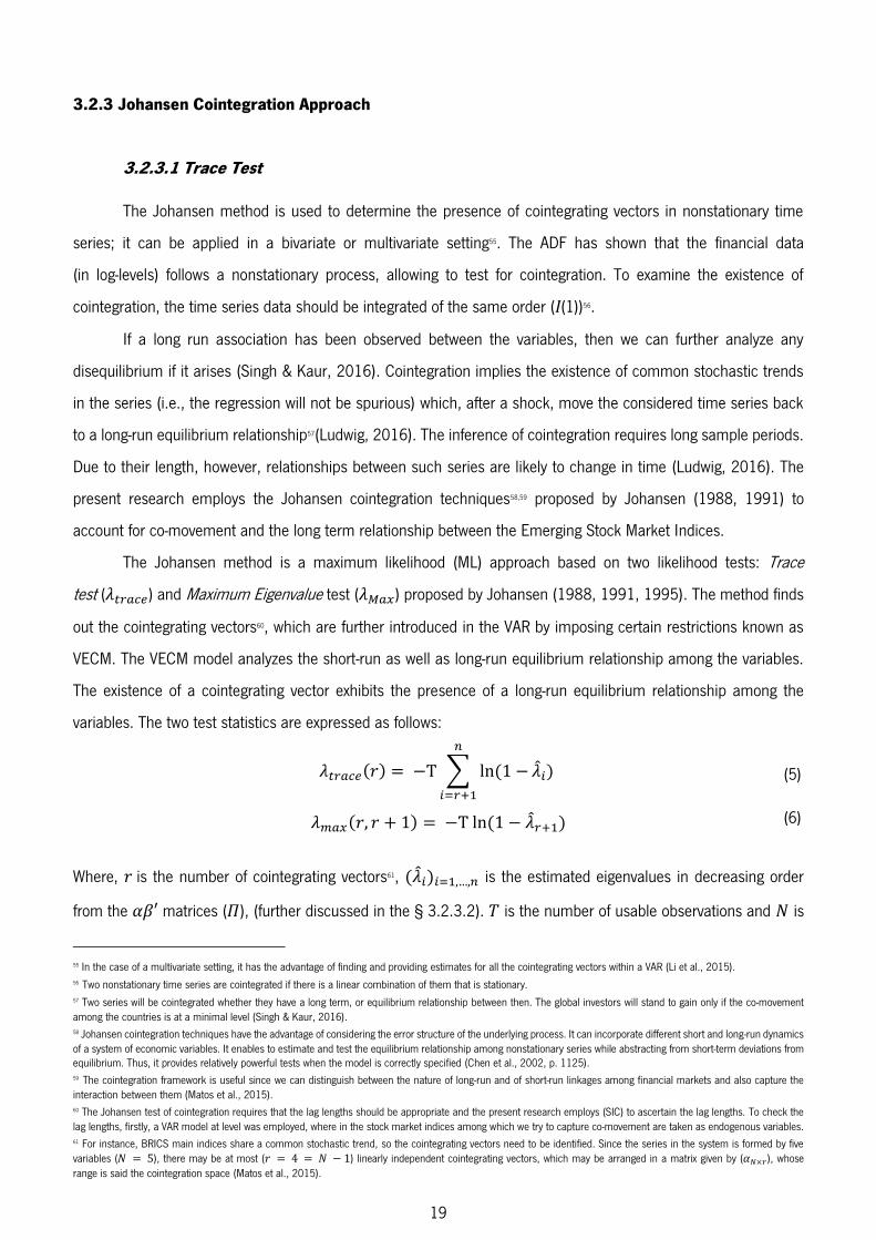
19

3.2.3 Johansen Cointegration Approach

3.2.3.1 Trace Test

The Johansen method is used to determine the presence of cointegrating vectors in nonstationary time

series; it can be applied in a bivariate or multivariate setting55. The ADF has shown that the financial data

(in log-levels) follows a nonstationary process, allowing to test for cointegration. To examine the existence of

cointegration, the time series data should be integrated of the same order (Ι(1))56.

If a long run association has been observed between the variables, then we can further analyze any

disequilibrium if it arises (Singh & Kaur, 2016). Cointegration implies the existence of common stochastic trends

in the series (i.e., the regression will not be spurious) which, after a shock, move the considered time series back

to a long-run equilibrium relationship57(Ludwig, 2016). The inference of cointegration requires long sample periods.

Due to their length, however, relationships between such series are likely to change in time (Ludwig, 2016). The

present research employs the Johansen cointegration techniques58,59 proposed by Johansen (1988, 1991) to

account for co-movement and the long term relationship between the Emerging Stock Market Indices.

The Johansen method is a maximum likelihood (ML) approach based on two likelihood tests: Trace

test ( ���) and Maximum Eigenvalue test ( ��) proposed by Johansen (1988, 1991, 1995). The method finds

out the cointegrating vectors60, which are further introduced in the VAR by imposing certain restrictions known as

VECM. The VECM model analyzes the short-run as well as long-run equilibrium relationship among the variables.

The existence of a cointegrating vector exhibits the presence of a long-run equilibrium relationship among the

variables. The two test statistics are expressed as follows:

��� = −T ∑ ln −= + ̂ �� , + = −T ln − ̂ +

Where, is the number of cointegrating vectors61, ̂ = ,…, is the estimated eigenvalues in decreasing order

from the ′ matrices (�), (further discussed in the § 3.2.3.2). � is the number of usable observations and � is

55 In the case of a multivariate setting, it has the advantage of finding and providing estimates for all the cointegrating vectors within a VAR (Li et al., 2015).

56 Two nonstationary time series are cointegrated if there is a linear combination of them that is stationary.

57 Two series will be cointegrated whether they have a long term, or equilibrium relationship between then. The global investors will stand to gain only if the co-movement

among the countries is at a minimal level (Singh & Kaur, 2016). 58 Johansen cointegration techniques have the advantage of considering the error structure of the underlying process. It can incorporate different short and long-run dynamics

of a system of economic variables. It enables to estimate and test the equilibrium relationship among nonstationary series while abstracting from short-term deviations from

equilibrium. Thus, it provides relatively powerful tests when the model is correctly specified (Chen et al., 2002, p. 1125). 59 The cointegration framework is useful since we can distinguish between the nature of long-run and of short-run linkages among financial markets and also capture the

interaction between them (Matos et al., 2015). 60 The Johansen test of cointegration requires that the lag lengths should be appropriate and the present research employs (SIC) to ascertain the lag lengths. To check the

lag lengths, firstly, a VAR model at level was employed, where in the stock market indices among which we try to capture co-movement are taken as endogenous variables. 61 For instance, BRICS main indices share a common stochastic trend, so the cointegrating vectors need to be identified. Since the series in the system is formed by five

variables (� = ), there may be at most ( = = � − ) linearly independent cointegrating vectors, which may be arranged in a matrix given by ( × ), whose

range is said the cointegration space (Matos et al., 2015).

(6)

(5)

20

the number of variables. Under the Trace test, the null hypothesis is there is no cointegrating vector ( : = ),

whereas the alternative hypothesis of cointegration is cointegrating vectors ( : > ). The Maximum

Eigenvalue test, tests the null hypothesis that the number of cointegrating vectors is equal to , whereas the

alternative hypothesis tests the number of cointegrating vectors as + . Hence, for each value of , for the given

orders: = , , , . . . � − , the test statistic is compared to the critical value to determine the number of

cointegrating vectors. If the test statistic is greater than the critical value, then the null hypothesis of =

cointegrating vector is rejected in favor of the alternative hypothesis = . If the test statistic is lower than the

critical value, however, the null hypothesis of no cointegrating vectors is not rejected. In this research, the ���

statistic is preferable to the �� statistic as it is more robust to deviations from the assumption of normally

distributed errors (Cheung & Lai, 1993). Moreover, the research of Rahbek, Hansen, and Dennis (2002) shows

that the trace statistic is robust so as to moderate the ARCH effect and, according to Juselius (2007), the choice

of rank should take into account all relevant information given by different criteria (trace test statistics, root of the

companion matrix) and especially the economic relevance of the results (Gentile & Giordano, 2012). Hence, we

focus solely on the trace test in our research to test for cointegration, as we can see in the next section below.

3.2.3.2 Dynamic Bivariate Cointegration Analysis

According to Gentile and Giordano (2013), the financial literature has shown in recent years that during a

crisis, new cointegration relationships among markets appear, which were not observed during tranquil periods of

time. These new long-run links generally involve countries which have a relevant role in the spreading out of

contagion (Arshanapalli, Doukas, & Lang, 1995; Click & Plummer, 2005; Jang & Sul, 2002; Ludwig, 2014; Malliaris

& Urrutia, 1992; Sander & Kleimeier, 2003; Sheng &Tu, 2000; Yang, Kolari, & Min, 2003). Consequently, we use

a bivariate dynamic cointegration analysis62 to test for the presence of new long-run equilibrium conditions among

countries through the application of dynamic rolling cointegration analysis63 for each pair of countries. Any increase

of the percentage of cointegrated countries over the total number of possible pairs signals a shift of the shock

transmission channels64 and represents the first indicator of potential contagion. According to the results obtained

in this step, it is possible to detect contagion windows by looking directly into the data, finding evidence which either

62 To individuate significant connections among pairs of markets, the bivariate Johansen cointegration test is applied to allows the identification of relations between pairs of

markets which lead to slow price adjustment processes – long-run connections (Gentile & Giordano, 2012, 2013). 63 To this end, most studies apply the rolling trace test. For recent contributions, see Mylonidis and Kollias (2010) and Peri and Baldi (2013). The rolling cointegration

analysis can be considered more appropriate than the alternative recursive analysis, because when conducting rolling window tests the size of subsamples is kept constant,

and both the first and the last observation in the subsamples roll through until the full sample is reached. That is, the test statistics are calculated for a rolling observations

time window by adding one observation to the end and removing the first observation and so on. Therefore, continuous plots of trace test statistics for a rolling, fixed length,

window provides essential information about the time varying pattern of the number of cointegrating vectors (i.e., to estimate the cointegration rank in the VECM, rolling

trace statistics enable the empirical researcher to graphically display the evolution of the cointegration rank (Ludwig, 2014). As in the case of recursive tests, the statistics

obtained from the rolling cointegration tests are scaled by the adjusted critical values of the chosen significance level are plotted (Mylonidis & Kollias, 2010, p. 2060). The

rolling window technique allows for the emergence of a clearer picture of the possible dynamic linkages among the stock markets as, although the sample size remains

unchanged, the sample period moves ahead by one observation at a time. In other words, the rolling estimation with a fixed-length window can ensure that the effects of

regime shifts are isolated and can be used to track possible structural breaks (Mylonidis & Kollias, 2010, p. 2060). 64 We defined “shift” as a significant increase in cross-market co-movements after a shock, not related with fundamentals links (Gentile & Giordano, 2012).

21

confirms or rejects the assumption of the time periods during which the contagion process could have started to

propagate during the two financial crises analyzed – LBBC and ESDC (Gentile & Giordano, 2012).

In the first step, following Gentile and Giordano (2012, 2013), we performed a pairwise countries rolling

cointegration estimation for the BRICS stock returns in order to verify whether there has been contagion during the

sample period by estimating at each point of time the number of markets long-run connections. A sharp increase

in the number of cross-market connections signals a contagion phenomenon. According to the results obtained in

this step, we detect the contagion window by looking directly to the data.

In order to determine the number of cointegrating equations, a VECM( ) was applied according to

Johansen (1988):

∆ = + ∑ ,�= Δ − + ∑ ,�

= Δ − + ′ [ −− ] + ,

∆ = � + ∑ ,�= Δ − + ∑ ,�

= Δ − + ′ [ −− ] + ,

Where, ∆ and ∆ are daily changes of stock returns referred to markets and , and are the

correspondent log-price indices (in log-level). The long-run impact matrix can be expressed as � = ′, where ′ = [ , ], and [ , ] is a vector of white noise processes. The vector of coefficient contains the

parameters of the common stochastic trend, while and measure the speed of convergence. In particular, ′ [ �−�− ] represents a common stochastic trend towards which price dynamic slowly converges. Hence, the

Johansen cointegration test mainly relies on the assumption that the rank of � equals the number of cointegrating

vectors. If the matrix � has a rank , there are cointegrating relations. When = , there is no long-run relation

among international markets and the Equation 7 would be reduced to a VAR(k).

Now, for detecting possible periods of contagion, the above dynamic Johansen cointegration test is applied

between all the possible pairs of countries65 with a rolling window of 1000-days66, by computing at each step ( ,

represents each month) of the procedure the following rolling indicator of cross-country connections:

� − � = − �� −� � ×

65 The sample in our research is formed by five ( = ) Emerging countries, therefore we have 10 pair of combinations in total, that is given by the following formula: !! − ! = !! − ! = , see Gómez-Puig and Sosvilla-Rivero (2014, 2011, p. 13).

66 The length of 1000 days-window (see Web Appendix 1 at https://sites.google.com/site/aguiarconraria/BRICS_WebAppendixes.pdf) is chosen in order to make

the cointegration results more robust, allowing to explore the asymptotic properties of the Johannsen test (Gentile & Giordano, 2012, 2013). Arce, Mayordomo, and

Peña (2012), used a 1000 days-window to consider a higher number of price-discovery metrics per day. Further, in the presence of autocorrelation coefficients, the power

of the trace test is as low as the nominal size for a window length of 250 days and becomes acceptable for windows of at least 1,000 days – four years (Ludwig, 2014, p.

19).

(7)

(8)

22

Using the rolling indicator in Equation 8, it is possible to discriminate as follows:

➢ Crisis periods are identified recording the highest values of cross-country connections.

➢ Tranquil periods are identified recording the lowest values of cross-country connections.

By comparing these highest and lowest percentage values, it may be possible to either confirm or reject

the assumption made regarding the timing of the two crises episodes investigated: Contagion occurs when cross-

country co-movements (percentage of cointegrated countries – known as cross-country connections), increase

during the crisis periods relative to cross-country connections during the tranquil periods.

3.2.4 Granger Causality Approach

3.2.4.1 Shock Transmission Direction

The second step of our research is obtained through the Granger causality test and VECM/Gonzalo-Granger

statistic (further discussed in §3.2.4.2), evaluating the significance of short-run connections between countries in

addition to the long-run equilibrium detected in the previous step by the cointegration analysis (see § 3.2.3.2 and

Web Appendix 4). Therefore, Granger causality methodology detects the versus67 (short and long-run causality) of

these connections, allowing to examine how shocks are transmitted through countries68. An increase of Granger

causality connections detected after a crisis period is a signal of contagion phenomenon. Hence, together with the

short-run versus of the connections, the detection of the long-run versus of the countries connections is also very

important and reached by implementing the Gonzalo-Granger statistic, allowing the identification of the direction of

connections in the crisis episodes.

Figure 2: Source: Author’s own. Framework implementation of the Granger Causality Methodology.

In this section, following Gentile and Giordano (2012, 2013), we have implemented the Granger causality

test because it allows one to investigate the short-run relationship among BRICS countries. The investigation

resorted to the long/short-run econometric techniques (Cointegration and Granger causality test) that allow one to

establish which country has a dominant role in the contagion process, being able to influence others

67 The versus of the long-run (cointegrated analysis) is two types of causality: short-run connections obtained by the Granger causality test and the long-run causality, which

is obtained in the context of the cointegration analysis based on the first step and it is applied in the Gonzalo-Granger statistic (see §3.2.4.2). 68 The granger causality test detects whether past values of the stock indices can predict future values of other stock indices. The estimation is conducted for each sub-

period (“contagion windows”) detected in the first step of the research according to Gentile and Giordano (2012, 2013).

Granger Analysis

Versus:

Short and Long-run Causality

Gonzalo-Granger Statistic

Direction of the Long-run Causality (VECM)

Granger-causality Test

Short-run Connections (VAR/VECM)

23

(“leading country”) and it allows one to identify of the most fragile country, in other words, it is possible to identify

the reaction of this country related to other countries’ price innovations (“follower country”). The method establishes

how much of the current value of can be explained by its past values and then to see whether adding values of

can improve the explanation.

In order to apply the Granger causality test, the following considerations were taken into account: first, the

time series were tested for unit root (see Web Appendix 3)69 in each sub-period established in the first step followed

by the cointegration test among pairs of countries (see Web Appendix 4). Second, the results of unit root test applied

earlier revealed that all the time series are nonstationary at log-level. However, the series are stationary at their first

difference ( (0)), that is, all the series are integrated of Order one ( (1)). Based on these results, if the series are

found to be ( (1)) and not cointegrated70, the causality test proceeded according to the following equations:

∆ = + ∑ ,= ∆ − + ∑ ,= ∆ − + , ∆ = + ∑ ,= ∆ − + ∑ ,= ∆ − + ,

However, if the series are found to be ( (1)) and cointegrated, causality test will be tested based on Equation 9. For

cointegrated series, different approaches to causality testing have to be applied. Based on results of Sims et al.

(1990), Demetriades and Hussein (1996) argue that test statistics derived from a level VAR framework are not valid

unless the variables employed are either ( (0)) or ( (1)) and cointegrated. This assumption drives the causality test

for Equation 9 if the series are not cointegrated. On the other hand, Engle and Granger (1987) and Granger (1988)

argue that in the presence of cointegration, causality tests derived from the cointegration relationship, which ignore

the ECT, are misspecified and suggest the re-parameterization of the model in the equivalent error correction model

form (VECM). Therefore, the causality test in this case is conducted in the following equations:

∆ = + ∑ ,= ∆ − + ∑ ,= ∆ − + � ��� , − + , ∆ = + ∑ ,= ∆ − + ∑ ,= ∆ − + � ��� , − + ,

The VECM-based test allows the differentiation between two types of causality: the short-run dynamics of the VAR

and the disequilibrium adjustment of the error correction mechanism (ECM). Indeed, the F-test on the estimated

69 All Web Appendixes are available at https://sites.google.com/site/aguiarconraria/BRICS_WebAppendixes.pdf. 70 The Equation 9 is only valid if the series are not cointegrated (MacDonald & Kearney, 1987).

(10)

(9)

24

coefficients provides evidence regarding a short-term adjustment dynamics. The t-test of the estimated coefficient � provides evidence for the existence of an arbitrage type error correction mechanism that drives the variables

back to their long-term equilibrium relationship that is embodied in the cointegration vector. In this step, the

objective is to identify the creation of new short-run relations among countries as evidence of contagion ( ),

conducting the Granger causality test separately for each contagion window (sub-periods defined in the first step)

based on the stock returns of all countries. Regarding the lag length71 , the criteria is chosen in order to generate

a white noise error term .

3.2.4.2 Common Factors/Price-Discovery/Permanent-Transitory Decomposition

Besides the short-run connections discussed previously, it is possible to reveal the other part of causality:

the long-run connections among the countries.

In order to detect the direction of the long-run causality among BRICS countries, we applied Gonzalo and

Granger (1995) methodology72 to identify the direction through which adjustment is done (see Web Appendix 5).

Hence, it is possible to estimate which country is the leader and which is the follower in the contagion transmission

in the context of a bivariate cointegration analysis (Engle & Granger, 1987). Furthermore, we can measure the

speed of convergence to the long-run equilibrium ( ) of the two hypothesized countries, while ( ) contains the

parameters of the common stochastic trend (Gentile & Giordano, 2012, 2013).

Gonzalo and Granger's model73 of price-discovery is based on the following VECM specification given by

Arce et al. (2012), adapted to our context (with USA stock return as a exogenous variable)74:

[∆∆ ] = ( − − − − −� − ) +[ ∑ , ΔX −�

=∑ , ΔX −�= ]

+[ ∑ , ΔY −�

=∑ , ΔY −�= ]

+[ ∑� ,��

= ∆ −�∑� ,��= ∆ −� ]

+ [ ,, ]

The above empirical model is a VAR system formed by two equations defined from the vector, which includes

and as the pair of BRICS stocks markets, , = Brazil, Russia, India, China, South Africa ( ≠ ); and an

error correction term (ECT) defined by the expression ( − − − − −� − ), where , and

71 The criteria information is given by the Akaike information criterion (AIC), the Schwartz information criterion (SIC), the Hannan-Quinn criterion (HQ) and the Likelihood

ratio statistic (LR). In this research, the SIC is preferable only when the serial correlation is not an issue. Otherwise, the preferable criterion will be the one that guarantees

no serial correlation. 72 The method proposed by Gonzalo and Granger decomposes the time series as: = ′ ′ + ⊥ ′⊥ ⊥ − ⊥ ; where ′ ′ is ( (0)) and the

transitory part, wile ⊥ ′⊥ ⊥ − ⊥ is ( (1)) and the permanent part (see Equation 11 in Gonzalo and Granger (1995)). The decomposition of the [ , ] into two

components (transitory and permanent), allow the obtainment of different kind of information. For example, policymakers may be primarily interested in the trend (permanent

component) behavior, but those concerned with business cycles are more interested in the cyclical component (transitory component). Moreover, singling out the common

factors allow us to investigate how they are related to other variables (Gonzalo & Granger, 1995). 73 The method is used to obtain the Matrix and Orthogonal Complement of and , extracting the Common Trends from a cointegration system according Gonzalo and

Granger (1995), for a better understanding (see Web Appendix 5 and 6). 74 As already mentioned, the variable USA is introduced in our model as an exogenous variable to account for the high influence that it has in the BRICS stock markets.

(11)

25

are estimated in an auxiliary cointegration regression and the parameter vector ′ = , contains the error

correction coefficients measuring each price’s expected speed of adjustment. The estimation of the VECM equation

is restricted to the existence of a cointegration relation between the stock market from both pair of countries. This

cointegration relation appears in the ECT as ( − − − − −� − ). The parameters λ , , λ , , δ , , , , ϑ , , and ϑ , for = ,… , with indicating the total number of lags, contain the coefficients of the VAR system

that measure the effect of the lagged75 first difference in the pair of stocks from BRICS countries markets based on

the first difference of such stocks at time . Finally, denotes a white noise vector , ~Ν , .

The price-discovery for the pair of stocks from the BRICS markets, denoted by and ,

respectively, can then be constructed from the elements of the vector ′, which contains the coefficients that

determine each market’s contribution to price-discovery:

= − = −−

Given that [ + = ], we would conclude that the � market leads the price-discovery process

whenever is higher(lower) than 0.5. The intuition for this is the faster the speed in eliminating the price

difference from the long-term equilibrium attributable to a given stock market, the higher the corresponding

according Equation 11, and the higher the price discovery (Arce et al., 2012).

At this point, we adapted Equation 12 to the view of Gentile and Giordano (2012, 2013), for instance,

assuming a pair of countries, as in the first step (see §3.2.3.2), the long-run coefficients matrix � in Equation 7

can be expressed as � = ′, where measures the speed of convergence to the long-run equilibrium of the two

hypothesized countries, while contains the parameters of the common stochastic trend. Furthermore, following

Equation 11, if the parameter of the speed adjustment of the first country ( ) is statistically not significant, while

the parameter of the speed adjustment of the second country ( ) is positive and significant, it means that the

adjustment process towards the long-term relationship is determined by changes to the variable of the second

country in response to changes of the variable of the first country, indicating that the leading role in the contagion

transmission is played by the first country. Otherwise, if ( ) is negative and statistically significant, while ( ) is

not significant, this implies that the second country plays the leading role. However, when both countries are

significant76, both countries contribute to the contagion transmission process and the Gonzalo-Granger statistic (see

Equation 12), defined as [ − ′], allows one to determine which country makes the greatest contribution to the

contagion transmission process. Hence, if the application of the ratio in Equation 12 for the first stock market

75 Lag order selection based on the lag order selection criteria (LR, AIC, SC, HQ) obtained in the VAR, which guarantees a model free of serial correlation by applying the

Autocorrelation LM test (See Web Appendix 6). 76 In that case, there is a shift of signals (Gentile & Giordano, 2012, 2013).

(12)

26

exceeds 0.5 (50%), the price of the first country plays a more important role, while if it is lower than 0.5, the price

of the second country plays a bigger role in the contagion transmission (Arce et al., 2012; Gentile &

Giordano, 2012).

3.2.4.3 VECM: Unveiling Two Types of Causality

This section is adapted from Gentile and Giordano (2012, 2013) methodology in order to detect two types

of causality by applying the VECM: the short-run dynamics of the VAR (identifying the short-term connections) and

the disequilibrium adjustment of the error correction mechanism (ECM) (identifying the direction of the connections)

for BRICS stock markets returns. Using the F-test on the estimated coefficients � , provides evidence of a short-

term adjustment dynamics, while the t-test of the estimated coefficient ′ provides evidence for the existence of

an arbitrage-type error correction mechanism that drives the variables back to their long-term equilibrium

relationship that is incorporated in the cointegration vector. In addition, the creation of new short-run relations

among countries reveals evidence of contagion (� , ).

The Granger causality test for the stock markets allows for the individualization of the short-term cross-

market links and it is based on the estimation of the multivariate cointegration model in which the dependent

variable is given by the stock return as follows77:

� = � + ∑���= � −� + ∑∑� ,�

== � − + ′[ l�� � −�l�� � −l�� � −�l�� � −l�� � −l�� � −. � ]

Where, is the coefficient which measures the speed of convergence to the long-run equilibrium; is the vector

which contains the parameters of the common stochastic trend; and represent country indices: , = Brazil,

Russia, India, China, South Africa ( ≠ ) and � is the number of countries included in the sample (� = 5). When

the time series are not cointegrated [ ′ = ], the model becomes a VAR(p)78. Otherwise, if the time series are

found to be cointegrated [ ′ ≠ ], then the model becomes a VECM(p). At this point, the USA stock index

returns79 is included in the model to test for Granger causality80. Regarding the synchronization issue, instead of

77 The model represented in Equation 13 embody the representation of the VAR (Equation 9) and VECM (Equation10), which can be seen separately and in more detail in

the (§ 3.2.4.1). 78 The order of the model is based on the application of Lag Order Selection Criteria. The priority is the elimination of the serial correlation. Hence, the chosen select

criterion is the (SIC), just when the serial correlation is not an issue. Otherwise, the selection is based on another referred criterion (AIC, HQ or LR). 79 Morgan Stanley Capital Index (MSCI) aggregate prices for USA based on the S&P 500 for Large Caps.

80 The inclusion of the USA stock market is necessary because, more comprehensive information is provided by including the USA market, indeed, linkage patterns between

the BRICS markets may be distorted when the influence of the USA market is not taken into consideration (Bekaert et al., 2011; Bonga-Bonga, 2015; Gentile &

Giordano, 2012, 2013; Mensah & Alagidede, 2017; Yang et al., 2003).

(13)

27

introducing the USA stock indices in the econometric model with one day lag delay ( − ) suggested by Malliaris

and Urrutia (1992), or applying two day rolling moving average suggested by Forbes and Rigobon (2002), the

chosen path to overcome the synchronization issue was to consider in the analysis a time window centered around

the two crises (LBBC and ESDC) as suggested by Jin and An (2016), rather than a single one.

The application of the Granger causality test allows one to find relevant short-term connections among

markets and to individuate the direction of these connections. For instance, if at least one � , for = ,… , is

significantly different from zero, this means that � influences � . In addition, throughout this methodology we are

able to find evidence of contagion, because this phenomenon amplifies the causality between markets following a

shock (Granger, 1969; Sander & Kleimeier, 2003).

3.2.5 Variance Decomposition: Exposure to External Shocks

The third step used in this research is dedicated to the forecast-error variance decomposition (FEVD), the

last contagion indicator, following Gentile and Giordano (2012, 2013). This methodology measures how much of

the movements in one country can be explained by shocks in other countries (applied in the stock market scenario).

Indicating that, as far as the proportion of the movements explained by other countries increases, the vulnerability

of the system also increases and becomes more exposed to external shocks (more exposed to external markets).

Following the conceptual framework discussed previously, at this point, our assumption is that contagion occurs

every time the degree of vulnerability of one country – measured as the fraction of its movements due to another

country’s shocks – increases after a crisis period.

The FEVD, looking from the econometric point of view, measures the fraction of the forecast-error variance

of an endogenous variable that can be attributed to orthogonalized shocks themselves or to another endogenous

variable, giving the portion of the movements in the dependent variables that are due to their “own” shocks, versus

shocks to the other variables81.

Initially, the FEVD indicator is given by the moving-average representation of the VECM as follows:

� = ∑� −∞=

Where, the , - ℎ component of � represents the impulse-response of the - ℎ country in periods to a shock

of one standard error in the - ℎ country, and is the orthogonalized innovation in the sense that it has an identity

81 A shock to the - ℎ variable will directly affect that variable; however, it will also be transmitted to all other variables in the system through the dynamic structure of the

VAR. Variance decompositions determine how much of the s-step-forward forecast error variance of a given variable is explained by innovations to each other explanatory

variables for = , , ,… , �.

28

covariance matrix. Initiating from this mathematical representation of the stock return, the variance of the -

forward forecast variance of the - ℎ return time series [� , + ] is given as follows:

� = ∑� ,= + ⋯ + ∑� ,=

Where, � is the number of countries included in the sample (� = )82. For each country stock market the ratio:

= ∑ � ,=�

represents the portion of movements in country due to shocks from country , on the time horizon . Therefore,

for [ = ] the ratio is as follows:

= ∑ � ,=�

indicating the portion of its forecast error variance which is explained by its own innovations. Consequently, its

complement to one [ − ] is the rate of involvement indicator, which measures the degree of vulnerability of

country , since it is the percentage of the variance of country explained by innovations in other countries, being

considered as a measure of country exposure to external shocks. In more detail, the rate of involvement – measures

the degree of vulnerability of each country, as a degree of exposure to the external shocks – indicating how much

“domestic” risk is explained by innovation in foreign countries.

82 Brazil, Russia, India, China and South Africa.

29

4 Results

4.1 Contagion Windows Definition

In our first-step results, we started by analyzing the connections among the BRICS markets through time.

At each point of time ( = each month)83, we estimated the linkages across markets. These linkages are able to

influence and determine the stock returns between the BRICS stock markets. A sharp increase of cross-market

connections signals a contagion phenomenon, as we can see in Figure 3 below.

Using a 1000-days84 rolling window and the dynamic bivariate cointegration test, in the first of the

three-step analysis, we detected the connections between markets (long-run relationships) that lead to slow price

adjustment processes. Further, applying the rolling indicator (Percentage of connections in Fig. 3, see Eq. 8

§3.2.3.2), it is possible to detect the increasing or decreasing connections between markets that can confirm the

assumption of tranquil or turbulent period of crisis. To identify these periods, the results of the rolling indicator are

combined with the quartiles85 to divide and set the precise timing of the contagion window by looking directly in the

data in order to define when the contagion phenomenon started to spread between the two financial crises (LBBC

and ESDC)86. Supposing the rolling indicator exceeds the III° quartile (Upper Bound - IIIº % =% ), the percentage of relevant connections is considered significantly high and, therefore, the period is

considered as turbulent. On the other hand, supposing the percentage of connections is high (but does not exceed

the IIIº) and there are no significant changes in the number of connections, then we assume it as evidence of

interdependence rather than contagion phenomenon (Gentile & Giordano, 2012, 2013). Therefore, the so called

“tranquil” period is identified as equal or under the IIIº quartile until the Iº quartile87 (Lower Bound -

Iº % = % ). Consequently, the “crisis” period is identified when the rolling indicator reveals a

higher percentage of connections above the upper bound and the “tranquil” period is given when the rolling

indicator reveals a lower percentage of connections equal to the IIIº quartile (but without significant changes in the

number of connections, indicating high interdependence) or below until the Iº quartile (lower bound).

83 The results contemplate in total 121 months and consequently, 121 rolling window in total (see Web Appendix 1).

84 In order to start (at the beginning of the month) and finish (at the end of the month), the rolling window was applied in an interval between [999;1002] days (see Web

Appendix 1 and 2). 85 The use of quantiles to identify significant increases (abnormal) of asset price co-movements, is justified by recent econometrics techniques (Caporin et al., 2013; Gentile

& Giordano, 2012, 2013; Koenker, 2005; Koenker, Ng, & Portnoy, 1994; Mensi et al., 2014). 86 Constâncio (2012, p. 110) and Caporin et al. (2013) maintain that a contagious event cannot occur in the absent of a shock, a large shock should occur. Enforcing the

finds in this research in line with other studies. See for example, Fourie and Botha ( 2015) and Gentile and Giordano (2012, 2013). 87 The median was taken in consideration to define the contagion window because most of the connections obtained from the rolling indicator is above the Iº quartile, which

indicates evidence of high co-movements, suggesting interdependence between the markets rather than contagion phenomenon.

4 Chapter

30

Figure 3: Graphical representation of the contagion window, using stock returns based on the results of the rolling indicator (see Web Appendix 2 for more details).

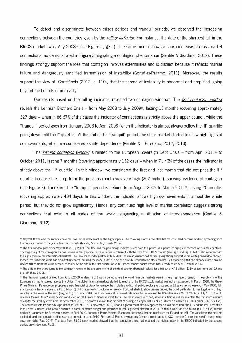
31

To detect and discriminate between crises periods and tranquil periods, we observed the increasing

connections between the countries given by the rolling indicator. For instance, the date of the sharpest fall in the

BRICS markets was May 200888 (see Figure 1, §3.1). The same month shows a sharp increase of cross-market

connections, as demonstrated in Figure 3, signaling a contagion phenomenon (Gentile & Giordano, 2012). These

findings strongly support the idea that contagion involves externalities and is distinct because it reflects market

failure and dangerously amplified transmission of instability (González-Páramo, 2011). Moreover, the results

support the view of Constâncio (2012, p. 110), that the spread of instability is abnormal and amplified, going

beyond the bounds of normality.

Our results based on the rolling indicator, revealed two contagion windows. The first contagion window

reveals the Lehman Brothers Crisis – from May 2008 to July 200989, lasting 15 months (covering approximately

327 days – when in 86,67% of the cases the indicator of connections is strictly above the upper bound), while the

“tranquil” period goes from January 2003 to April 2008 (when the indicator is almost always bellow the IIIº quartile

going down until the Iº quartile). At the end of the “tranquil” period, the stock market started to show high signs of

co-movements, which we considered as interdependence (Gentile & Giordano, 2012, 2013).

The second contagion window is related to the European Sovereign Debt Crisis – from April 201190 to

October 2011, lasting 7 months (covering approximately 152 days – when in 71,43% of the cases the indicator is

strictly above the IIIº quartile). In this window, we considered the first and last month that did not pass the IIIº

quartile because the jump from the previous month was very high (20% higher), showing evidence of contagion

(see Figure 3). Therefore, the “tranquil” period is defined from August 2009 to March 201191, lasting 20 months

(covering approximately 434 days). In this window, the indicator shows high co-movements in almost the whole

period, but they do not grow significantly. Hence, any continued high level of market correlation suggests strong

connections that exist in all states of the world, suggesting a situation of interdependence (Gentile &

Giordano, 2012).

88 May 2008 was also the month where the Dow Jones index reached the highest peak. The following months revealed that the crisis had become evident, spreading from

the housing market to the global financial markets (Mollah, Zafirov, & Quoresh, 2014).

89 The first window goes from May 2008 to July 2009. The data and the percentage indicator evidenced this period as a period of highly connections across the countries.

The beginning of the contagion window shown in the graphical representation is coherent with the data from BRICS market (see Fig.1 and Fig.3), but is also coherent with

the signs given by the international markets. The Dow Jones index peaked in May 2008, as already mentioned earlier, giving strong support to the contagion window chosen.

Indeed, the subprime crisis had devastating effects, bursting the global asset bubble and quickly jumped to the stock market. By October 2008 it had already erased around

US$25 trillion from the value of stock markets. At the end of the first quarter of 2009, global market capitalization had already fallen 53% (Chittedi, 2014). 90 The date of the sharp jump to the contagion refers to the announcement of the third country (Portugal) asking for a bailout of €78 billion ($110 billion) from the EU and

the IMF (Ray, 2015). 91 The “tranquil” period defined from August 2009 to March 2011 was a period where the world financial markets were in a very high level of tension. The problems of the

Eurozone started to spread across the Union. The global financial markets started to react and the BRICS stock market was not an exception. In March 2010, the Greek

Prime Minister (Papandreou) proposes a new financial package for Greece that includes additional public sector pay cuts and a 2% sales tax increase. On May 2010, IMF

and Eurozone leaders agree to a €110 billion ($143 billion) bailout package for Greece. Portugal starts to show vulnerabilities, the bond yields start to rise together with high

volatility in the value of the euro (Ray, 2015). On June 2010, the Euro closes at its lowest rate of exchange against the US dollar since March 2006. In July 2010, the EU

releases the results of “stress tests” conducted on 91 European financial institutions. The results were very bad, seven institutions did not maintain the minimum amount

of capital required by examiners. In September 2010, it becomes known that the cost of bailing out Anglo Irish Bank could reach as much as €34.3 billion ($46.6 billion). The results elevate Ireland’s budget deficit to 32% of GDP. In November 2010, Ireland’s government officially applies for bailout funds from the EU and the IMF. Embattled

Irish Prime Minister Brian Cowen submits a harsh austerity budget and promises to call a general election in 2011. Within a week an €85 billion ($113 billion) rescue package is approved by European leaders. In April 2010, Portugal’s Prime Minister (Socrates), requests a bailout relief from the EU and the IMF. The volatility in the markets

exploded, and the contagion effect starts to spread. In June 2010, Standard & Poor’s downgrades Greece’s credit rating to CCC, turning Greece the world’s lowest-rated

sovereign debt (Ray, 2015). The data from BRICS stock market showed that the contagion effect had reached the highest peak in the ESDC indicated by the second

contagion window (see Fig.3).

32

Figure 4: Graphical representation of the percentage of significant connections (rolling indicator), computed by applying a moving average of two months (MA2) and four months (MA4).

33

Connections between the stock returns are always above the median, but it is still reasonable to consider

them the result of interdependence and not contagion.

In Figure 4 we present the total amount of possible relationships obtained from the rolling indicator for the

BRICS stock returns. Figure 4 shows and highlights the differences in the pattern of crisis, making it possible to

see the pattern of Subprime Crisis separately from the LBBC by applying the MA of two and four months.

The intensity of cross-market connections given by the rolling indicator shows a different pattern related to

the stock market return, identifying two contagion episodes. The first one begins around May 2008 and ends around

July 2009, including consequently, both the Subprime and Lehman Bankruptcy Crisis. The indicator shows that

the peak is achieved in March and April 2009, reaching 100% of cross-market linkages as significant92 (see

Figure 3). The second contagion window pointing to the ESDC, from April to October 2009, reaches a peak of cross-

market linkages of 70%. However, the intensity of this crisis was much smaller and shorter in the BRICS economies

than the first one related to the LBBC.

Table 4 Contagion Window Summary

Stock Market Returns

Lehman Brothers Bankruptcy Crisis European Sovereign Debt Crisis

Duration: 15 Months Duration: 7 Months

01/05/2008 - 31/07/2009:

Approximately 327 days. In 86,67%93 of the cases the rolling

indicator is strictly above the upper bound IIIº Quartile (Θ °%).

01/04/2011 - 31/10/2011:

Approximately 152 days. In 71,43% of the cases the rolling

indicator is strictly above the upper bound IIIº Quartile (Θ °%).

In Table 4 the results of the contagion window are summarized. The results will be used in the next part of

the research to analyze the contagion process inside the windows, comparing whether the number of cross-market

connections in “crisis” period increases compared to the “tranquil” period. The first part of our research has

considered until now just the long-run connections, implying just the slow price adjustment process given by the

Johansen cointegration test. However, to verify the presence of a contagion effect, the total number of connections

(long-run and short-run connections) is needed. For that purpose, the Granger causality test, the so called second

step of our analysis will be applied, as we can see in the next section.

4.2 Revealing the Contagion Process

In our second step results, we analyze the results arising from the number of cross-market connections

related with the “crisis” periods and compare them with the “tranquil” periods, by applying the cointegration test

and the Granger causality test (see § 3.2.3.2 and §3.2.4.1). The bivariate cointegration test allows the identification

92 Revealing that the intensity of the crisis in BRICS countries was deeper than in previous times (Mollah, Zafirov, & Quoresh, 2014).

93 Looking at Figure 3 §4.1, is possible to see 13 long-run connections out of 15 that are above the IIIº Quartile ( %). Dividing 13 by 15 long-run connections, the result

is 86,67% for the LBBC. The same is applied for the ESDC.

34

of connections between pairs of markets which lead to slow price adjustment process (long-run connections, see

Web Appendix 4). But it is also possible to find the versus of each significant connection by applying the Gonzalo-

Granger statistic (see § 3.2.4.2 and Web Appendix 5 and 6). Furthermore, the Granger causality test identifies

connections which have a short-term influence on the price discovery process (short-run connections)94, as

demonstrated by Gentile and Giordano (2012, 2013). In Table 5 we can see the Gonzalo-Granger results.

Table 5 Results from Cointegration Test/Gonzalo-Granger Statistics.

January 2003 to April 2008 - Tranquil period

Pair of Countries Gonzalo-Granger Statistic Speed of Adjustment [ ] Results

Leading/Follower Countries

BRAZIL - INDIA GGBRA -0.001675 Leading country GGIND 0.011453*** Follower country

May 2008 to July 2009 - Turbulent period: Subprime and Lehman Brothers Crisis

Pair of Countries Gonzalo-Granger Statistic Speed of Adjustment [ ] Results

Leading/Follower Countries

BRAZIL - CHINA GGBRA -0.004429 Leading country

GGCHI 0.044729*** Follower country

INDIA - CHINA GGIND -0.056525*** Follower country

GGCHI -0.002313 Leading country

INDIA - S. AFRICA GGIND -0.069595*** Follower country

GGSAF -0.002708 Leading country

CHINA - S. AFRICA GGCHI -0.146660*** Follower country

GGSAF 0.061711 Leading country

August 2009 to March 2011 - Tranquil period

Pair of Countries Gonzalo-Granger Statistic Speed of Adjustment [ ] Results

Leading/Follower Countries

BRAZIL - CHINA GGBRA -0.042440** Follower country

GGCHI 0.018214 Leading country

April 2011 to October 2011 - Turbulent period: European Sovereign Debt Crisis

Pair of Countries Gonzalo-Granger Statistic Speed of Adjustment [ ] Results

Leading/Follower Countries

BRAZIL - INDIA GGBRA -0.024887 Leading country

GGIND 0.117500*** Follower country

BRAZIL - CHINA GGBRA 0.015320 Leading country

GGCHI 0.157903*** Follower country

BRAZIL - S. AFRICA GGBRA 0.258053*** Leading country GGSAF 0.237389*** Leading country

RUSSIA - S. AFRICA GGRUS 0.081265 Leading country

GGSAF 0.150673*** Follower country

INDIA - S. AFRICA GGIND -0.085531* Follower country

GGSAF 0.093486 Leading country

CHINA - S. AFRICA GGCHI 0.023620 Leading country GGSAF 0.200972*** Follower country

Note: Source Author’s on based on the imputes from EVIEWS 9.0 Program. The results obtained from the VECM in the context of the Granger causality

test (see Web Appendix 5 and 6) allow the obtainment of the speed of adjustment of the first country (α ) and second country (α ) respectively, in other

words, the coefficients of error correction terms. [***] indicates the level of significance at 1% level; [**] at 5% level; [*] at 10% level. [ ] represents the

leading country that makes the greatest contribution to the contagion transmission process. Besides this, the line in bold indicates which country makes

the greatest contribution to the contagion by applying the Gonzalo-Granger statistic [ αα −α ′]. In this context, if the ratio for the first country exceeds

0.5, the first country plays a bigger role in the contagion transmission, while if the ratio is lower than 0.5 (the maximum is 1), the opposite is true (Gentile

& Giordano, 2012).

94 See (§3.2.4.3) for econometric details and Web Appendix 6.

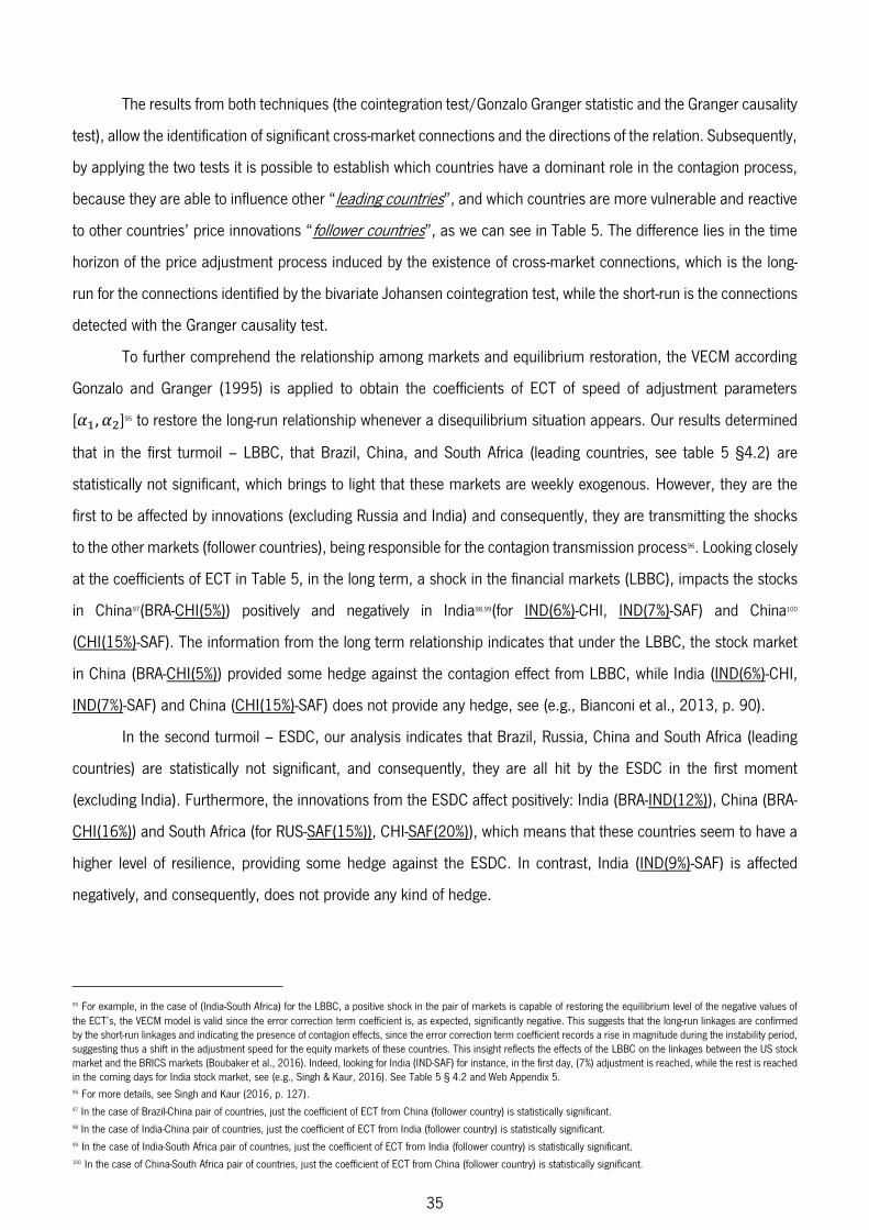
35

The results from both techniques (the cointegration test/Gonzalo Granger statistic and the Granger causality

test), allow the identification of significant cross-market connections and the directions of the relation. Subsequently,

by applying the two tests it is possible to establish which countries have a dominant role in the contagion process,

because they are able to influence other “leading countries”, and which countries are more vulnerable and reactive

to other countries’ price innovations “follower countries”, as we can see in Table 5. The difference lies in the time

horizon of the price adjustment process induced by the existence of cross-market connections, which is the long-

run for the connections identified by the bivariate Johansen cointegration test, while the short-run is the connections

detected with the Granger causality test.

To further comprehend the relationship among markets and equilibrium restoration, the VECM according

Gonzalo and Granger (1995) is applied to obtain the coefficients of ECT of speed of adjustment parameters

[ , ]95 to restore the long-run relationship whenever a disequilibrium situation appears. Our results determined

that in the first turmoil – LBBC, that Brazil, China, and South Africa (leading countries, see table 5 §4.2) are

statistically not significant, which brings to light that these markets are weekly exogenous. However, they are the

first to be affected by innovations (excluding Russia and India) and consequently, they are transmitting the shocks

to the other markets (follower countries), being responsible for the contagion transmission process96. Looking closely

at the coefficients of ECT in Table 5, in the long term, a shock in the financial markets (LBBC), impacts the stocks

in China97(BRA-CHI(5%)) positively and negatively in India98,99(for IND(6%)-CHI, IND(7%)-SAF) and China100

(CHI(15%)-SAF). The information from the long term relationship indicates that under the LBBC, the stock market

in China (BRA-CHI(5%)) provided some hedge against the contagion effect from LBBC, while India (IND(6%)-CHI,

IND(7%)-SAF) and China (CHI(15%)-SAF) does not provide any hedge, see (e.g., Bianconi et al., 2013, p. 90).

In the second turmoil – ESDC, our analysis indicates that Brazil, Russia, China and South Africa (leading

countries) are statistically not significant, and consequently, they are all hit by the ESDC in the first moment

(excluding India). Furthermore, the innovations from the ESDC affect positively: India (BRA-IND(12%)), China (BRA-

CHI(16%)) and South Africa (for RUS-SAF(15%)), CHI-SAF(20%)), which means that these countries seem to have a

higher level of resilience, providing some hedge against the ESDC. In contrast, India (IND(9%)-SAF) is affected

negatively, and consequently, does not provide any kind of hedge.

95 For example, in the case of (India-South Africa) for the LBBC, a positive shock in the pair of markets is capable of restoring the equilibrium level of the negative values of

the ECT’s, the VECM model is valid since the error correction term coefficient is, as expected, significantly negative. This suggests that the long-run linkages are confirmed

by the short-run linkages and indicating the presence of contagion effects, since the error correction term coefficient records a rise in magnitude during the instability period,

suggesting thus a shift in the adjustment speed for the equity markets of these countries. This insight reflects the effects of the LBBC on the linkages between the US stock

market and the BRICS markets (Boubaker et al., 2016). Indeed, looking for India (IND-SAF) for instance, in the first day, (7%) adjustment is reached, while the rest is reached

in the coming days for India stock market, see (e.g., Singh & Kaur, 2016). See Table 5 § 4.2 and Web Appendix 5. 96 For more details, see Singh and Kaur (2016, p. 127).

97 In the case of Brazil-China pair of countries, just the coefficient of ECT from China (follower country) is statistically significant.

98 In the case of India-China pair of countries, just the coefficient of ECT from India (follower country) is statistically significant.

99 In the case of India-South Africa pair of countries, just the coefficient of ECT from India (follower country) is statistically significant.

100 In the case of China-South Africa pair of countries, just the coefficient of ECT from China (follower country) is statistically significant.

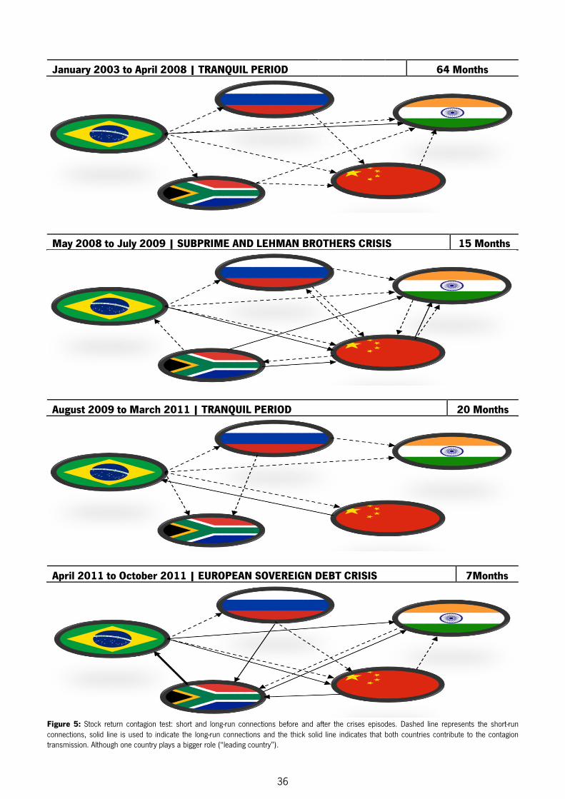
36

January 2003 to April 2008 | TRANQUIL PERIOD 64 Months

May 2008 to July 2009 | SUBPRIME AND LEHMAN BROTHERS CRISIS 15 Months

August 2009 to March 2011 | TRANQUIL PERIOD 20 Months

April 2011 to October 2011 | EUROPEAN SOVEREIGN DEBT CRISIS 7Months

Figure 5: Stock return contagion test: short and long-run connections before and after the crises episodes. Dashed line represents the short-run

connections, solid line is used to indicate the long-run connections and the thick solid line indicates that both countries contribute to the contagion

transmission. Although one country plays a bigger role (“leading country”).

37

Figure 5 shows the long and short-run relations among the stock returns markets and the direction of these

connections (Figure 5 derived from Web Appendix 7), revealing the structure of the contagion propagation

mechanism. Hence, when the connections are statistically relevant, the results from the test statistic are reported

together with its significance level (see Web Appendix 7) by following Gentile and Giordano (2012, 2013).

Analyzing the results of long and short connections among the markets, it is possible to notice that Brazil,

China and South Africa dominated the stock market during the LBBC as leading countries (May 2008 to July 2009)

and the number of cross-markets connections increased sharply from 8 (January 2003 to April 2008) to 12 (May

2008 to July 2009). Thereafter, when the analysis is directed to the ESDC (April 2011 to October 2011), the

number of cross-market connections increased from 7 (August 2009 to March 2011) to 10 (April 2011 to October

2011), wherein, China clearly lost the dominant role in the contagion transmission played in the Lehman Crisis.

Regarding Brazil and South Africa, Brazil is the major leading country in the ESDC, playing a dominant role in the

contagion transmission structure by influencing Russia, India, China (both short/long-run) and South Africa101 stock

markets; it is followed by South Africa with much less intensity, playing a leading role in Brazil and India stock

markets. Indeed, in 2008-09, Brazil was able to influence the stock returns of all other countries except for South

Africa together with China. The latter was, in turn, able to influence all other countries excepted for Brazil.

A higher dominant role can be seen in the ESDC for the Brazil stock market (now influencing also South

Africa, see Web Appendix 7, Table 5 and Figure 5), while for China, the dominant role of influencing other markets

diminished clearly. In 2008-09, China had a dominant role in the contagion transmission by influencing Russia,

India (both short/long-run) and South Africa, whereas in the ESDC it just leads the South Africa stock market,

maintaining the connection only with the India stock market. Furthermore, South Africa, which during the LBBC

had been able to influence Brazil, India and China stock markets, in the recent ESDC, it was only capable of

influencing Brazil and India, losing the dominant role in transmitting contagion to China's stock market.

Regarding the LBBC, it is possible to analyze that Brazil and China were the greatest leading countries in

the contagion transmission, followed by South Africa, whereas in the ESDC only Brazil stock market kept the

strength, playing a dominant role in the contagion process. However, in the first crisis, there is evidence of high

connections concentrated in the leading countries (Brazil, China and South Africa); while in the second crisis the

evidence point towards for a dominant role in the contagion transmission mechanism coming strongly from Brazil,

with much less intensity from South Africa and lastly, the contagion transmission running from China and Russia

to South Africa market. In 2008-09 crisis, the number of relevant connections involving India and China is higher

compared to what was observed in the latest crisis, where India and South Africa presented the same amount of

connections. Indeed, in the Lehman Crisis, Russia and India absorbed shocks without being able to influence other

countries (pure follower country), signaling a high degree of vulnerability. In the case of China, this market absorbed

101 The result in absolute value did not exceed 0.5 for Brazil (-11,48805). For South Africa, the value (12,488047) exceeded in absolute value 0.5. Therefore, the price of

the second asset (South Africa (SAF)), plays a bigger role compared to the first asset (Brazil (BRA)), see Table 5 above.

38

shocks but also spread them, while in the case of Brazil, which is a major contributor to the contagion transmission

(even in tranquil periods of times), was highly capable of spreading shocks to all other countries (in both crises)

and was not influenced by any of them, excepting for South Africa in both crises. Despite being a pure follower

country in the first crisis, Russia lost this role in the latest crisis, playing a leading role in South Africa. India

continued to be a pure follower country, not being able to lead any country, but receiving shocks from all of them,

revealing a high level of vulnerability in both crisis.

Our results also reveal the risk profile of India and China in the LBBC as sharply higher compared to the

other countries based on the number of relevant connections. Therefore, the contagion process is mainly related

to India and China stock markets. While in the ESDC, the risk profile of India and South Africa is the same but lower

than the previous crisis, indicating that the process of contagion is mainly related with these two countries, with

Brazil as a major source in spreading the contagion to all BRICS stock markets in both crises. One difference

between the two crises considered (LBBC and ESDC) that clearly emerges, is related to the amount of short-run

connections during LBBC (10 short-run connections over 14 total connections) compared to the ESDC (5 short-run

connections over 11 total connections). Moreover, it seems that the LBBC is characterized by a strong increase in

the number of short-run links, while the ESDC is characterized by a higher level of long-run connections (7 long-run

links102 over 11 total connections). Overall, it seems that the LBBC was able to affect more intensively the BRICS

markets than the ESDC. Although, the ESDC seems to be less severe but more dispersed between the BRICS

countries, the contagion transmission seems to be more dangerous, due to the fact that all countries are

transmitting/spreading the contagion to each other (with exception for India).

The most important result from this analysis is related to the confirmation of the existence of contagion as

opposed to interdependence or spillover. The number of connections detected among countries (in both contagion

windows), increased after the “crisis episodes” but did not remain at such a high level after the shock. Indeed, the

number of connections increased intensively during “crisis periods” and then decreased drastically during “tranquil

periods”. This movement is a critical test to distinguish between contagion and interdependence. As stated earlier

in this research, contagion is a significant increase in the co-movement between assets during a period of crisis,

compared with a tranquil period. Therefore, if there is a high level of market co-movement in all periods, that is the

case of interdependence. As it is possible to see in this research (see Figure 3 and Figure 4, §4.1), a higher number

of connections in the BRICS stock markets which do not hold steady after a shock, returning to the low values once

the crisis is gone, is a signal of a temporary distortion of the transmission channels due to shocks – that is contagion,

instead of a systematic change in the common economic structure, based on the real or financial links103 (Gentile

& Giordano, 2012, 2013).

102 The Brazil influence over South Africa, even though weaker, was considered at this point (see Table 5).

103 These theories are usually based on standard transmission mechanisms, such as trade, monetary policy, and common shocks, for example, oil prices (Gentile &

Giordano, 2012; Kishor & Singh, 2014; Nikkinen, Saleem, & Martikainen, 2013).

39

4.3 Measuring Countries Degree of Exposure to the Contagion Process

The last step is reached by applying the variance decomposition methodology, following Gentile and

Giordano (2012, 2013). This methodology allows us to measure of each country’s degree of exposure to the

influence of foreign markets, indicating the rate of involvement in the contagion process (see §3.2.5). Furthermore,

the results in Table 6 below reveal that South Africa is incredibly more significantly involved in the ESDC compared

with its involvement in the LBBC. Indeed, all the BRICS countries exhibited a significant increase in the involvement

of the contagion process in the second crisis ESDC. Regarding South Africa, for a time frame of 5 days (short term),

the ratio of the forecast error variance (the rate of involvement indicator104) explained by foreign markets increased

from 2.82% (LBBC) to 31.32% (ESDC), making South Africa the most involved country in the contagion process

with the highest degree of exposure to external shocks followed by India (from 11.27% to 27.30%), Russia (from

9.21% to 24%), China (from 21% to 31.36%) and Brazil (from 4.87% to 14.26%), with the lower degree of exposure

to the contagion process105.

Directing the analysis to the two crises considered, the variance decomposition methodology provides an

insight about the contagion intensity for the countries in the sample. For instance, during the LBBC, the most

involved country in the contagion process was China, the degree of exposure rose (from 12.92% to 21%)106 after the

crisis, much higher than the other countries. Still in the LBBC window, it is interesting to notice that South Africa

represented the lowest level of vulnerability (from 9.23% to 2.82%), followed by India (from 11.82% to 11.27%),

indicating that these two countries seem to have a strong degree of exogeneity to the system, not being affected

essentially by the LBBC compared to the other countries107. Concerning the ESDC, in the short-term, the most

exposed country to external shocks and consequently more vulnerable and involved in the contagion process is

South Africa (from 6.52% to 31.32%), followed by Russia (from 9.31% to 24%), India (from 14.52% to 27.30%),

Brazil (from 2.08% to 14.26%) and lastly, China (from 24.24% to 31.36%)108.

Summarizing, in the LBBC China was the most affected country in terms of degree of exposition to external

markets (21% for the short period and 28.19% for the long period) and in terms of growth rate of vulnerability before

and after the first crisis (from 12.92% to 21% for the short period and from 13.42% to 28.19% for the long period).

104 The degree of vulnerability of each country (Gentile & Giordano, 2013). 105 Reaching a growth rate of vulnerability of 28.50%(South Africa), followed by 16.03%(India), 14.79%(Russia), 10.36%(China) and 9.39%(Brazil). The percentage is calculated

taking the difference between the last crisis (ESDC) minus the ratio of the first crisis (LBBC), as it is possible to see in Table 6 for 5 days forecast. In the long period, South

Africa remains the most vulnerable country, reaching a growth rate of vulnerability of 55.54%, followed by 41.56% (Russia in the long period, overtakes India), 37.96%(India),

33.31%(Brazil) and lastly, 22.19%(China). 106 Followed by Brazil (from 2.16% to 4.87%) and by Russia (from 7.72% to 9.21%).

107 Looking at the long period, for South Africa (from 14.28% to 4.15%), Russia (from 12.17% to 9.44%) and Brazil (from 6.26% to 5.14%) was essentially unaffected in the

LBBC, whereas for India (from 14.75% to 17.86%) there was an increase in the vulnerability to external shocks. As regards South Africa, the results indicate that it is even

more unaffected compared to the short period. 108 In the ESDC, all countries become sharply more exposed to external shocks. Therefore, South Africa records the most severe worsening of external fragility, reaching a

growth rate of vulnerability of 24.80%, followed by Russia (14.69%), India and Brazil (with nearly the same rate of involvement, 12.78% and 12.18%) and China with (7.12%),

the least fragile country. In the long period, South Africa remains the most fragile country, reaching a growth rate of vulnerability of 53.29%, but in the case of Russia

(37.09%), Brazil (36.19%) and India (35.91%), the external fragility is almost the same, indicating that in the long period these countries are equally affected by external

shocks, with the same rate of involvement in the Sovereign Debt Crisis. Lastly, China is the least fragile country with a growth rate of vulnerability of 17.78%.

40

Focusing the analysis on the ESDC, our results highlight that South Africa, Russia, India and Brazil are

countries more exposed to financial contagion, mostly because of their higher degree of fragility (31.32%, 24%,

27.30% and 14.26%) in the short period, while for the long period the degree of fragility was (59.69%, 51%, 38.45%

and 55.82%) for South Africa, Russia, Brazil and India, respectively. Furthermore, China records the worst

performance in terms of rise of rate of involvement, mostly because of its high pre-Lehman vulnerability (from

24.24% to 31.36% for the short period; and from 32.60% to 50.38% for the long period). Comparing both crises in

terms of growth rate of vulnerability, the results indicate that South Africa is the most exposed to the financial

contagion (28.50% for the short period; and 55.54% for the long period), followed by India (16.03%) and Russia

(14.79%) in the short period. In the long period, Russia (41.56%) overtakes India (37.96%), becoming more exposed

to the financial contagion than India, followed by Brazil with a growth rate of vulnerability of (33.31%), indicating a

large increase in the degree of exposition to external markets in contrast with the short period.

Table 6 Rate of Exposure to the Contagion Process based on the Stock Returns.

Countries Forecast Horizon (Days)

Tranquil period

Pre-Lehman Bankruptcy

Turbulent period

Lehman Bankruptcy

Tranquil period

Pre-Sovereign Debt Crisis

Turbulent period

EU Sovereign Debt Crisis

Df1 Df2 Df3

Brazil 5 2.16 4.87 2.71 2.08 14.26 12.18 9.39

10 6.26 5.14 -1.12 2.26 38.45 36.19 33.31

Russia 5 7.72 9.21 1.49 9.31 24.00 14.69 14.79

10 12.17 9.44 -2.73 13.91 51.00 37.09 41.56

India 5 11.82 11.27 -0.55 14.52 27.30 12.78 16.03

10 14.75 17.86 3.11 19.91 55.82 35.91 37.96

China 5 12.92 21.00 8.08 24.24 31.36 7.12 10.36

10 13.42 28.19 14.77 32.60 50.38 17.78 22.19

S. Africa 5 9.23 2.82 -6.41 6.52 31.32 24.80 28.50

10 14.28 4.15 -10.13 6.40 59.69 53.29 55.54

Note: Source Author’s on based on the imputes from EVIEWS 9.0 Program. The results are presented in percentage. The variance decomposition was

computed based on a 5 (short period) and 10 days (long period) forecast horizon. The Table 6 indicates the rate of involvement indicator [ − �� � ], measuring the degree of vulnerability of country �(each country’s stock market) explained by innovations in all other countries, working as a measure of

country’s exposure to the external shocks (see §3.2.5). [Df1] represents the difference between tranquil and turbulent period in the Lehman Crisis. [Df2]

represents the difference between tranquil and turbulent period in the Sovereign Debt Crisis and [Df3] represents the difference between both crises. For

the results of each country’s contribution to the contagion process individually (see Web Appendix 8).

4.4 Three-steps Results: Summary of the Major Findings

The main results obtained in sections: 4.1, 4.2 and 4.3 are summarized in Table 7 using stock market

returns.

Equally noteworthy, is the fact that in our research, the results corroborate many more short-run linkages

than long-run connections. The short connections are higher due to the nature of equity prices – shorter-term and

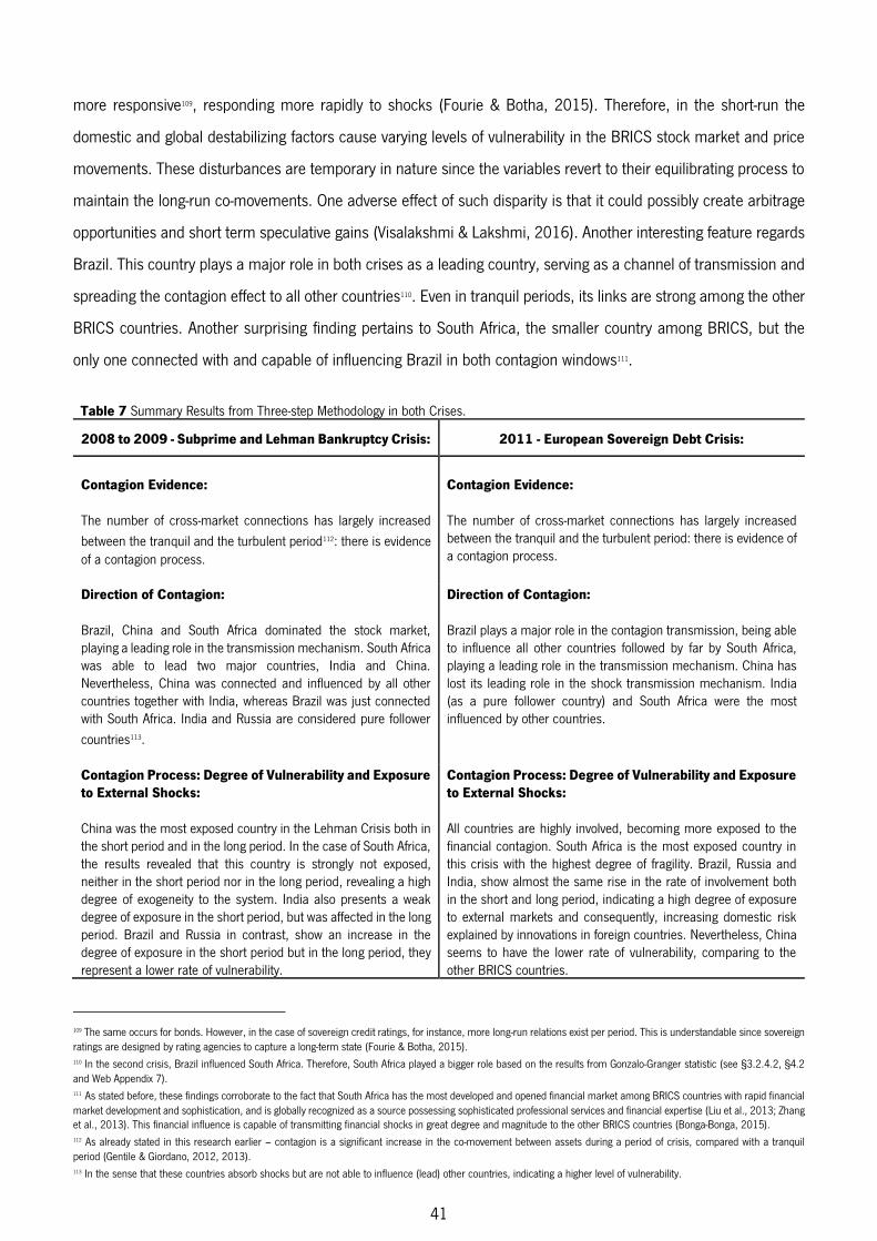
41

more responsive109, responding more rapidly to shocks (Fourie & Botha, 2015). Therefore, in the short-run the

domestic and global destabilizing factors cause varying levels of vulnerability in the BRICS stock market and price

movements. These disturbances are temporary in nature since the variables revert to their equilibrating process to

maintain the long-run co-movements. One adverse effect of such disparity is that it could possibly create arbitrage

opportunities and short term speculative gains (Visalakshmi & Lakshmi, 2016). Another interesting feature regards

Brazil. This country plays a major role in both crises as a leading country, serving as a channel of transmission and

spreading the contagion effect to all other countries110. Even in tranquil periods, its links are strong among the other

BRICS countries. Another surprising finding pertains to South Africa, the smaller country among BRICS, but the

only one connected with and capable of influencing Brazil in both contagion windows111.

Table 7 Summary Results from Three-step Methodology in both Crises.

2008 to 2009 - Subprime and Lehman Bankruptcy Crisis: 2011 - European Sovereign Debt Crisis:

Contagion Evidence: The number of cross-market connections has largely increased

between the tranquil and the turbulent period112: there is evidence

of a contagion process.

Contagion Evidence: The number of cross-market connections has largely increased

between the tranquil and the turbulent period: there is evidence of

a contagion process.

Direction of Contagion: Brazil, China and South Africa dominated the stock market,

playing a leading role in the transmission mechanism. South Africa

was able to lead two major countries, India and China.

Nevertheless, China was connected and influenced by all other

countries together with India, whereas Brazil was just connected

with South Africa. India and Russia are considered pure follower

countries113.

Direction of Contagion: Brazil plays a major role in the contagion transmission, being able

to influence all other countries followed by far by South Africa,

playing a leading role in the transmission mechanism. China has

lost its leading role in the shock transmission mechanism. India

(as a pure follower country) and South Africa were the most

influenced by other countries.

Contagion Process: Degree of Vulnerability and Exposure to External Shocks: China was the most exposed country in the Lehman Crisis both in

the short period and in the long period. In the case of South Africa,

the results revealed that this country is strongly not exposed,

neither in the short period nor in the long period, revealing a high

degree of exogeneity to the system. India also presents a weak

degree of exposure in the short period, but was affected in the long

period. Brazil and Russia in contrast, show an increase in the

degree of exposure in the short period but in the long period, they

represent a lower rate of vulnerability.

Contagion Process: Degree of Vulnerability and Exposure to External Shocks: All countries are highly involved, becoming more exposed to the

financial contagion. South Africa is the most exposed country in

this crisis with the highest degree of fragility. Brazil, Russia and

India, show almost the same rise in the rate of involvement both

in the short and long period, indicating a high degree of exposure

to external markets and consequently, increasing domestic risk

explained by innovations in foreign countries. Nevertheless, China

seems to have the lower rate of vulnerability, comparing to the

other BRICS countries.

109 The same occurs for bonds. However, in the case of sovereign credit ratings, for instance, more long-run relations exist per period. This is understandable since sovereign

ratings are designed by rating agencies to capture a long-term state (Fourie & Botha, 2015). 110 In the second crisis, Brazil influenced South Africa. Therefore, South Africa played a bigger role based on the results from Gonzalo-Granger statistic (see §3.2.4.2, §4.2

and Web Appendix 7). 111

As stated before, these findings corroborate to the fact that South Africa has the most developed and opened financial market among BRICS countries with rapid financial

market development and sophistication, and is globally recognized as a source possessing sophisticated professional services and financial expertise (Liu et al., 2013; Zhang

et al., 2013). This financial influence is capable of transmitting financial shocks in great degree and magnitude to the other BRICS countries (Bonga-Bonga, 2015). 112 As already stated in this research earlier – contagion is a significant increase in the co-movement between assets during a period of crisis, compared with a tranquil

period (Gentile & Giordano, 2012, 2013). 113 In the sense that these countries absorb shocks but are not able to influence (lead) other countries, indicating a higher level of vulnerability.

42

5 Conclusions

The contagion effect in the financial markets has been reinforcing the concerns in emerging and advanced

economies, mostly after the large impact that started with the collapse of the USA mortgage market in 2007

(Subprime Crisis), triggering the financial turmoil in global markets materialized in a GFC114 after the Lehman

Brothers Collapse, causing a massive devaluation in the global markets. To make matters worse, the GFC

undermined the economies around the world, spreading and becoming more severe in some regions, revealing the

weakness in economies around the globe, for instance in Europe, the GFC triggered the ESDC, another major crisis,

that was capable of transmitting massive shocks throughout the financial markets.

Our research contributes to a better understanding of the contagion phenomenon115 by analyzing the

changes in cross-market connections for the BRICS stock markets. The application of VECM cointegration and

Granger causality methodology detected the contagion in order to measure shifts in the shocks transmission

channels caused by the creation of new long-run equilibrium together with the raising of new short-run

connections116, by analyzing changes in the long/short-run connections in both contagion windows (LBBC and

ESDC).

Our results reveal that there was a contagion effect phenomenon in both crises117, given that the number

of cross-market connections increased sharply after such crises events occurred and reduced afterwards118. A new

long-run equilibrium relationship between BRICS markets was created, causing a deterioration of the diversification

benefits in both crises compared to the tranquil times (i.e., the presence of a cointegrating vector indicates long-

114 However, the impact was in varying proportion depending on the internal strength of the economy of the individual BRICS countries. The crisis spread to the BRICS

through all four channels: trade, finance, commodity and confidence channels. In Brazil, the local currency and stock market has seen huge fluctuation as foreign investment

(see Appendix III) has gone down, demand for commodity export dried up and external credit decreased, the financial markets in Russian froze due to a rise in risk aversion

and sudden change in exchange rate expectation which was triggered by the collapse of oil prices in September 2008 led the Russian banks and firms to seek to hedge

their foreign currency exposure which led to pressure on the ruble. In the Indian economy, there was fall in GDP growth rate and external demand shock had a larger impact

on output and employment. Impact of the financial crisis on China took the form of decrease in external demand which led to economic slowdown and rising unemployment.

In case of South Africa, portfolio inflows had accounted for the bulk of financing of South Africa’s large CAD (Current Account Deficit) which led to large net outflows, both

export and import volumes felled which affected South Africa’s main export commodities weakened. The global financial crisis inflicted significant loss in output in all the

BRICS economies (Kishor & Singh, 2014, p. 415). 115 One of the main interest of contagion studies is concerned to the international portfolio diversification. Theoretically, diversification reduce portfolio risk, but when cross-

country correlations increase during crises, this concept is undermined. Understanding financial contagion would clearly be beneficial for police makers in order to prevent

future spreads of crises according to Gentile and Giordano (2012). 116 The significant rising in the short-run connections is evidence of contagion. This phenomenon amplifies the causality between markets followed by a shock (Boubaker et

al., 2016). 117 Although BRIC (excluding South Africa) economies have heterogeneous profiles in terms of the cultural, political, social, demographic and macroeconomic contexts, or

also observing human capital and labor market variables, the evidence corroborates with previous studies suggesting that their main stock market indices share short and

long-run equilibrium relationships, thus indicating the evidence of the exist of high levels of integration and contagion. For more details, see Matos et al. (2015). 118 As stated in Gentile and Giordano (2012, 2013), contagion occurs when cross-country co-movements (represented by the percentage of cointegrated countries), increase

during crisis periods and decrease in the tranquil periods. Hence cannot be explained by fundamentals, which involves just interdependence. In other words, how different

the propagation of shocks is after a large negative realization has taken place (Edwards, 2000).

5 Chapter

43

run relationship among the countries concerned during the crisis period. The co-movement reduces diversification

benefits for the investors (Singh & Kaur, 2016, p. 126)). By applying the Granger causality119, our results point to

changes in the short-run linkages between BRICS markets. These results confirm the transmission of shocks from

the LBBC and ESDC to BRICS stock markets existed and was amplified during the crisis period120. In fact, shocks

from the LBBC and ESDC affected the BRICS stock markets in the short-run, implying that only trivial opportunities

existed for diversifying risk of international investors. Furthermore, Brazil serve as a channel of contagion

transmission, receiving shocks from both crises and spreading them to the rest of the BRICS. Additionally,

movements from Brazil stock market, could serve as an indicator to predict behaviors in other BRICS markets.

The VECM/Gonzalo-Granger statistic121 revealed, that Brazil played a bigger role as a leading country in the

transmission of the contagion to the other countries. It also Indicated also that India is the most vulnerable country

in both crises (a pure following country). Moreover, innovations from LBBC hit Brazil, China and South Africa first,

and consequently, they transmitted the contagion to the other countries. In this crisis, only China was able to

provide some hedge against shocks from LBBC. On the other hand, in the ESDC, Brazil, Russia, China and South

Africa were affected at same time, but in this crisis, the BRICS stock markets were able to be more resilient,

providing a better degree of hedge against the innovations from ESDC.

Regarding the degree of vulnerability of BRICS markets to external shocks, the evidence corroborates that

China was the most exposed country in the LBBC, whereas in the ESDC, all countries presented a higher degree

of exposure and fragility, with South Africa being the most fragile country and more exposed to the financial

contagion. These results bring great implications for the portfolio diversification in these markets. The effects of

contagion in the BRICS markets can change investors’ behavior, the financial stability can lead to high correlations

in the markets, and phenomena like “fight-to-quality” 122, “heard behavior” and "bandwagon" effects on the part of

investors123 may arise (Gentile & Giordano, 2012; Kazi & Wagan, 2014). However, it is interesting to notice an

increasing integration between BRICS countries, through a much deeper relationship and bilateral trade

agreements, which is opening their economies and financial sector. Their stock markets, however, are not fully

cointegrated, making them still independent from the global financial system, benefiting, for instance, the global

investors that intend to invest in the BRICS equity market indices to enjoy the diversification as well as international

exposure benefits (Singh & Kaur, 2016).

119 Our model includes the USA stock market as an exogenous variable, which was able to influence/Granger cause all the BRICS countries in all time windows.

120 Consequently, these findings suggest contagion effect and the sensitivity of the BRICS markets to news announcement from USA markets in the post-crisis

period (Boubaker et al., 2016; Kishor & Singh, 2014). Indicating that investors can rely on lagged values of the USA equity prices as indicator to forecast the behavior of

BRICS stock markets (Lakshmi et al., 2015, p. 317). 121 To a better understanding of these results (see table 5, §4.2).

122 As already mentioned, since the adopted definition of “shift” contagion relies on a significant increase in cross-market co-movements after a shock, which is not related

with fundamentals linkages (financial, real, political). The only transmission that could explain contagion is the behavioral one (Gentile & Giordano, 2012). 123 A form of group think, in which investor's probability of adopting any belief increases with the proportion who have already done so, hence investors do not discriminate

among economic fundamentals across countries.

44

In the last decades, the BRICS countries underwent an important process of trade and financial

liberalization to benefit from the advantages of market integration. Therefore, integrated financial markets allow,

investors to allocate consumption risk more efficiently, decreasing the costs of capital faced by firms and stimulating

investment and economic growth. However, the increased financial integration has intensified contagion effects

across markets, causing severe welfare losses for large geographical regions. Consequently, integrating a national

market with global financial markets may facilitate the transmission of international shocks to domestic stock

markets, having important implications for the decisions of investors’, risk managers, regulatory and monetary

authorities and in particular, consequences for effective portfolio diversification (Zouhair et al., 2014).

Several important policy and economic implications can be drawn from the empirical results of this study.

The evidence of the impact caused by both crises in the BRICS stock markets also provides meaningful insights

pertinent to international asset pricing, risk management and the dynamic interactions in the global economy. For

instance, gold's ability to act as a safe haven in the case of South Africa may have financial implications regarding

the presence of diversification opportunities during extreme market conditions. With the “financialization” of the

commodity markets, gold and oil can provide further protection against losses when the traditional assets (equities

and bonds) experience large declines. Thus, including commodities in traditional portfolios that include BRICS

markets, allow investors to avoid the downside risk in their investments. Gold can also provide protection against

dollar devaluations (Mensi et al., 2014). This research is also particularly helpful for portfolio risk managers, energy

traders, policymakers and international investors who should be cautious about making investments in

simultaneous markets that exhibit pure contagion. Knowledge of dependencies of the BRICS is crucial for

policymakers to help them discern the directions of the co-movements and to safe guard the BRICS stock markets

from contagion during future crises or major events.

Understanding the reasons of financial contagion between BRICS and international stock markets can help

policymakers to develop a prevailing financial system to make BRICS markets more immune to international shock

transmission, limiting their exposure to the contagion effects by improving stock market liquidity, as the BRICS

markets increasingly become more integrated with the international markets.

45

References

Ahmad, W., Sehgal, S., & Bhanumurthy, N. R. (2013). Eurozone Crisis and BRIICKS Stock Markets: Contagion or Market

Interdependence? Economic Modelling, 33, 209–225.

Aloui, R., Aïssa, M. S. Ben, & Nguyen, D. K. (2011). Global financial crisis, extreme interdependences, and contagion effects:

The role of economic structure? Journal of Banking & Finance, 35(1), 130–141.

Andenmatten, S., & Brill, F. (2011). Measuring Co-Movements of CDS Premia during the Greek Debt Crisis. University of Bern, Department of Economics Discussion Papers, 1–36.

Ang, A., & Chen, J. (2002). Asymmetric Correlations of Equity Portfolios. Journal of Financial Economics, 63(3), 443–494.

Arce, O., Mayordomo, S., & Peña, J. I. (2012). Credit-Risk Valuation in the Sovereign CDS and Bonds Markets: Evidence from the Euro Area Crisis (No. 53). CNMV - Spanish Securities Markets Commission.

Arshanapalli, B., Doukas, J., & Lang, L. H. P. (1995). Pre and Post-October 1987 Stock Market Linkages between U.S. and

Asian Markets. Pacific Basin Finance Journal, 3(1), 57–73.

Bae, K.-H., Karolyi, G. A., & Stulz, R. M. (2000). A New Approach to Measuring Financial Contagion (No. 7913). NBER Working Papers.

Bae, K.-H., Karolyi, G. A., & Stulz, R. M. (2003). A New Approach to Measuring Financial Contagion. The Review of Financial Studies, 16(3), 717–763.

Baig, T., & Goldfajn, I. (1999). Financial Market Contagion in the Asian Crisis. International Monetary Fund Staff Papers,

46(2), 167–195.

Baur, D. G. (2012). Financial contagion and the real economy. Journal of Banking & Finance, 36(10), 2680–2692.

Beirne, J., & Gieck, J. (2012). Interdependence and Contagion in Global Asset Markets (No. 1480). ECB - Working Paper Series.

Bejarano-Bejarano, L. V., Gomez-Gonzalez, J. E., Melo-Velandia, L. F., & Torres-Gorron, J. E. (2015). Financial Contagion in Latin America (No. 884). Borradores de Economía. Banco de la República.

Bekaert, G., Ehrmann, M., Fratzscher, M., & Mehl, A. (2011). Global Crises and Equity Market Contagion (No. 1381). ECB Working Paper Series. European Central Bank.

Bekaert, G., & Harvey, C. R. (1995). Time-Varying World Market Integration. The Journal of Finance, 50(2), 403–444.

Bekaert, G., Harvey, C. R., & Ng, A. (2005). Market Integration and Contagion. Journal of Business, 78(1), 39–70.

Bekiros, S. D. (2014). Contagion, decoupling and the spillover effects of the US financial crisis: Evidence from the BRIC

markets. International Review of Financial Analysis, 33, 58–69.

Ben Rejeb, A., & Boughrara, A. (2015). Financial integration in emerging market economies: Effects on volatility transmission

and contagion. Borsa Istanbul Review, 15(3), 161–179.

Berger, D., & Pukthuanthong, K. (2012). Market fragility and international market crashes. Journal of Financial Economics,

105(3), 565–580.

Bianconi, M., Yoshino, J. A., & Machado de Sousa, M. O. (2013). BRIC and the U.S. Financial Crisis: An Empirical Investigation

of Stock and Bond Markets. Emerging Markets Review, 14, 76–109.

Bonga-Bonga, L. (2015). Uncovering equity market contagion among BRICS countries: an application of the multivariate GARCH model (No. 66262). MPRA Paper.

Bordo, M. D., & Murshid, A. P. (2000). Are Financial Crises Becoming Increasingly More Contagious? What is the Historical Evidence on Contagion? (No. w7900). NEBER Working Paper Series. Cambridge, MA.

Boubaker, S., Jouini, J., & Lahiani, A. (2016). Financial contagion between the US and selected developed and emerging

countries: The case of the subprime crisis. The Quarterly Review of Economics and Finance, 61, 14–28.

Boyer, K. and Y. (2006). How Do Crises Spread? Evidence from Accessible and Inaccessible Stock Indices. The Journal of Finance, 61(2), 957–1003.

Brooks, C. (2008). Introductory Econometrics for Finance (2nd ed.). Cambridge: Cambridge University Press.

Broto, C., & Pérez-Quirós, G. (2015). Disentangling contagion among sovereign CDS spreads during the European debt crisis.

Journal of Empirical Finance, 32, 165–179.

Campbell, R., Forbes, C. S., Koedijk, K., & Kofman, P. (2006). Diversification Meltdown or Just Fat Tails? University of Maastricht, 1–38.

Caporin, M., Pelizzon, L., Ravazzolo, F., & Rigobon, R. (2013). Measuring Sovereign Contagion in Europe (No. 18741). NBER Working Papers. Cambridge, MA.

Chen, G., Firth, M., & Meng Rui, O. (2002). Stock market linkages: Evidence from Latin America. Journal of Banking & Finance, 26(6), 1113–1141.

46

Cheung, Y.-W., & Lai, K. S. (1993). Finite-Sample Sizes of Johansen’s Likelihood Ratio Tests for Cointegration. Oxford Bulletin of Economics and Statistics, 55(3), 313–328.

Chiang, T. C., Jeon, B. N., & Li, H. (2007). Dynamic correlation analysis of financial contagion: Evidence from Asian markets.

Journal of International Money and Finance, 26(7), 1206–1228.

Chittedi, K. R. (2014). Global Financial Crisis and Contagion: Evidence for the “BRIC” Economies*. The Journal of Developing Areas, 48(4), 243–264.

Claessens, S., Dornbusch, R., & Park, Y. C. (2001). Contagion: Why Crises Spread and How This Can Be Stopped. In S.

Claessens & K. J. Forbes (Eds.), International Financial Contagion (pp. 19–42). Boston, MA: Springer US.

Click, R., & Plummer, M. G. (2005). Stock Market Integration in ASEAN. Journal of Asian Economics, 16(1), 5–28.

Constâncio, V. (2012). Contagion and the European debt crisis. Banque de France - Financial Stability Review, 109–121.

Corsetti, G., Pericoli, M., & Sbracia, M. (2001). Correlation Analysis of Financial Contagion: What One Should Know Before Running a Test (No. 822). Economic Growth Center (EGC). Economic Growth Center, Yale University.

Corsetti, G., Pericoli, M., & Sbracia, M. (2005). Some Contagion, some Interdependence: More Pitfalls in Tests of Financial

Contagion. Jounal of International Money and Finance, 24, 1177–1199.

Cronin, D., Flavin, T. J., & Sheenan, L. (2016). Contagion in Eurozone sovereign bond markets? The good, the bad and the ugly. Economics Letters (Vol. 143).

Demetriades, P. O., & Hussein, K. A. (1996). Does financial development cause economic growth? Time-series evidence from

16 countries. Journal of Development Economics, 51(2), 387–411.

Dickey, D. A., & Fuller, W. A. (1979). Distribution of the Estimators for Autoregressive Time Series With a Unit Root. Journal of the American Statistical Association, 74(366), 427–431.

Dickey, D. A., & Fuller, W. A. (1981). Likelihood ratio statistics for autoregressive time series with a unit root. Econometrica,

49(4), 1057–1072.

Diebold, F., & Yilmaz, K. (2008). Measuring Financial Asset Return and Volatility Spillovers, With Application to Global Equity Markets (No. 13811). NBER Working Paper Series. Cambridge, MA.

Dornbusch, R., Park, Y. C., & Claessens, S. (2000). Contagion: Understanding How It Spreads. The World Bank Research Observer, 15(2), 177–197.

Dungey, M., & Martin, V. L. (2007). Unravelling financial market linkages during crises. Journal of Applied Econometrics,

22(1), 89–119.

Dungey, M., & Yalama, A. (2010). Detecting Contagion with Correlation: Volatility and Timing Matter (No. 35). Centre for Financial Analysis & Policy. Cambridge Judge Business School, University of Cambridge.

Edwards, S. (2000). Contagion. The World Economy, 23(7), 873–900.

Eichengreen, B., Rose, A. K., & Wyplosz, C. (1996). Contagious Currency Crises. Scandinavian Journal of Economics, 98(4),

463–484.

Enders, W. (2010). Applied Econometric Time Series. (Wiley, Ed.) (3rd ed.). New York: John Wiley & Sons, Inc.

Engle, R. F., & Granger, C. W. J. (1987). Co-Integration and Error Correction: Representation, Estimation, and Testing.

Econometrica, 55(2), 251–276.

Favero, C. A., & Giavazzi, F. (2000). Looking for Contagion: Evidence from the ERM (No. 7797). NBER Working Papers Series.

Favero, C. A., & Giavazzi, F. (2002). Is the International Propagation of Financial Shocks Non-Linear? Journal of International Economics, 57(1), 231–246.

Forbes, K. J. (2012). The “Big C”: Identifying and Mitigating Contagion (No. 4970–12).

Forbes, K. J., & Rigobon, R. (1999). No Contagion, only Interdependence: Measuring Stock Market Co-movements (No. 7267).

NEBER Working Paper Series.

Forbes, K. J., & Rigobon, R. (2001). Measuring Contagion: Conceptual and Empirical Issues. In S. Claessens & K. J. Forbes

(Eds.), International Financial Contagion (pp. 43–66). Boston, MA: Springer US.

Forbes, K. J., & Rigobon, R. (2002). No Contagion, Only Interdependence: Measuring Stock Market Comovements. The Journal of Finance, 57(5), 2223–2261.

Fourie, L., & Botha, I. (2015). Sovereign Credit Rating Contagion in the EU. Procedia Economics and Finance, 24, 218–227.

Gentile, M., & Giordano, L. (2012). Financial Contagion during Lehman default and Sovereign Debt Crisis: An Empirical Analysis on Euro Area Bond and Equity Markets. Quaderni di Finanza CONSOB (Vol. 72).

Gentile, M., & Giordano, L. (2013). Financial Contagion during Lehman Default and Sovereign Debt Crisis. An Empirical

Analysis on Euro Area Bond and Equity Markets. Journal of Financial Management, Markets and Institutions, 1(2), 197–224.

Goldstein, M. (1998). The Asian Financial Crisis. Policy Briefs PB98-1.

Gómez-Puig, M., & Sosvilla-Rivero, S. (2014). EMU Sovereign Debt Market Crisis: Fundamentals-based or Pure Contagion? (No. 14–8). Asociación Española de Economía y Finanzas Internacionales.

47

Gómez-Puig, M., & Sosvilla-Rivero, S. J. (2011). Causality and Contagion in Peripheral EMU Public Debt Markets: A Dynamic Approach (No. 2011/16). Research Institute of Applied Economics (IREA).

González-Páramo, J. M. (2011). Sovereign Contagion in Europe. In Speaker Seminar of the European Economics and Financial Centre. London. Retrieved from http://www.mondovisione.com/media-and-resources/news/sovereign-contagion-in-

europe-speech-by-jos-manuel-gonzlez-pramo-member-of/

Gonzalo, J., & Granger, C. (1995). Estimation of Common Long-Memory Components in Cointegrated Systems. Journal of Business & Economic Statistics, 13(1), 27–35.

Granger, C. W. J. (1969). Investigating Causal Relations by Econometric Models and Cross-Spectral Methods. Econometrica,

37(3), 424–438.

Granger, C. W. J. (1988). Some recent development in a concept of causality. Journal of Econometrics, 39(1–2), 199–211.

IMF. (2016). World Economic Outlook Database April 2016. Retrieved November 20, 2016, from

https://www.imf.org/external/pubs/ft/weo/2016/01/weodata/index.aspx

Jang, H., & Sul, W. (2002). The Asian Financial Crisis and the Co-Movement of Asian Stock Markets. Journal of Asian Economics, 13(1), 94–104.

Jarque, C. M., & Bera, A. K. (1980). Efficient tests for normality, homoscedasticity and serial independence of regression

residuals. Economics Letters, 6(3), 255–259.

Jin, X., & An, X. (2016). Global financial crisis and emerging stock market contagion: A volatility impulse response function

approach. Research in International Business and Finance, 36, 179–195.

Johansen, S. (1988). Statistical analysis of cointegration vectors. Journal of Economic Dynamics and Control, 12(2), 231–254.

Johansen, S. (1991). Estimation and Hypothesis Testing of Cointegration Vectors in Gaussian Vector Autoregressive Models.

Econometrica, 59(6), 1551–1580.

Johansen, S. (1995). Likelihood-Based Inference in Cointegrated Vector Autoregressive Models. Oxford: Oxford University

Press.

Juselius, K. (2007). The Cointegrated VAR Model: Methodology and Applications (2nd ed.). Oxford University Press.

Kalbaska, A., & Gątkowski, M. (2012). Eurozone sovereign contagion: Evidence from the CDS market (2005–2010). Journal

of Economic Behavior & Organization, 83(3), 657–673.

Kaminsky, G. L., & Reinhart, C. M. (1998). Financial Crises in Asia and Latin America : Then and Now. The American

Economic Review, 88(2), 444–448.

Kaminsky, G. L., & Reinhart, C. M. (2000). On crises, contagion, and confusion. Journal of International Economics, 51(1),

145–168.

Kazi, I., & Wagan, H. (2014). Are emerging markets exposed to contagion from US: Evidence from stock and sovereign bond markets (No. 2014–58). Ipag - Working Paper Series.

Khalid, A. M., & Kawai, M. (2003). Was financial market contagion the source of economic crisis in Asia?: Evidence using a

multivariate VAR model. Journal of Asian Economics, 14(1), 131–156.

Kishor, N., & Singh, R. P. (2014). Stock Return Volatility Effect: Study of BRICS. Transnational Corporations Review, 6(4),

406–418.

Koenker, R. (2005). Quantile Regression. Econometric Society Monographs. New York: Cambridge University Press.

Koenker, R., Ng, P., & Portnoy, S. (1994). Quantile smoothing splines. Biometrika, 81(4), 673–680.

Lakshmi, P., Visalakshmi, S., & Shanmugam, K. (2015). Intensity of shock transmission amid US-BRICS markets.

International Journal of Emerging Markets, 10(3), 311–328.

Li, D. Y. W., Ho, A., & Yau, P. P. (2015). A Study on Stock Markets of Developing Countries’ Integration & Relevance with Developed Countries’ Stock Markets. Scholedge International Journal of Management & Development, 2(6), 61–70.

Liu, T., Hammoudeh, S., & Thompson, M. A. (2013). A momentum threshold model of stock prices and country risk ratings:

Evidence from BRICS countries. Journal of International Financial Markets, Institutions and Money, 27(1), 99–112.

Ljung, G. M., & Box, G. E. P. (1978). On a measure of lack of fit in time series models. Biometrika, 65(2), 297–303.

Luchtenberg, K. F., & Vu, Q. V. (2015). The 2008 financial crisis: Stock market contagion and its determinants. Research in International Business and Finance, 33, 178–203.

Ludwig, A. (2014). What results can we expect from rolling trace tests? A discussion based on the issue of stock market

integration. Economics Bulletin, 34(1), 16–24.

Ludwig, A. (2016). On the usability of the fluctuation test statistic to identify multiple cointegration break points. Journal of Applied Statistics, 43(9), 1604–1624.

MacDonald, R., & Kearney, C. (1987). On the specification of granger-causality tests using the cointegration methodology.

Economics Letters, 25(2), 149–153.

48

MacKinnon, J. G. (1996). Numerical distribution functions for unit root and cointegration tests. Journal of Applied Econometrics, 11(6), 601–618.

Malliaris, A. G., & Urrutia, J. L. (1992). The International Crash of October 1987: Causality Tests. The Journal of Financial and Quantitative Analysis, 27(3), 353–364.

Masson, P. (1998). Contagion: Monsoonal Effects, Spillovers, and Jumps Between Multiple Equilibria (No. 98/142). IMF Working Paper.

Masson, P. (1999). Contagion: macroeconomic models with multiple equilibria. Journal of International Money and Finance,

18(4), 587–602.

Matos, P., Oquendo, R., & Trompieri, N. (2015). Integration and Contagion of BRIC Financial Markets (2015/02). NCF Researching Paper Series.

Mensah, J. O., & Alagidede, P. (2017). How are Africa’s emerging stock markets related to advanced markets? Evidence from copulas. Economic Modelling, 60, 1–10.

Mensi, W., Hammoudeh, S., Reboredo, J. C., & Nguyen, D. K. (2014). Do global factors impact BRICS stock markets? A

quantile regression approach. Emerging Markets Review, 19, 1–17.

Mollah, S., Zafirov, G., & Quoresh, A. S. (2014). Financial Market Contagion during the Global Financial Crisis (No. 2014/5).

Center for Innovation and Technology Research.

Mollah, S., Zafirov, G., & Quoreshi, A. S. (2014). Financial Market Contagion during the Global Financial Crisis (No. 2014/5).

CITR Working Paper Series. Center for Innovation and Technology Research, Blekinge Institute of Technology.

Moser, T. (2003). What Is International Financial Contagion? International Finance, 6(2), 157–178.

Muratori, U. (2014). Contagion in the Euro Area Sovereign Bond Market. Social Sciences, 4(1), 66–82.

Mylonidis, N., & Kollias, C. (2010). Dynamic European Stock Market Convergence: Evidence from Rolling Cointegration

Analysis in the First Euro-Decade. Journal of Banking & Finance, 34(9), 2056–2064.

New Delhi. (2012). The BRICS Report. Oxford University press.

Nikkinen, J., Saleem, K., & Martikainen, M. (2013). Transmission of the Sbprime Crisis: Evidence from Industrial and Financial

Sectors of BRIC Countries. Journal of Applied Business Research, 29(5), 1469–1478.

Nistor, P. (2015). FDI Implications on BRICS Economy Growth. Procedia Economics and Finance, 32(15), 981–985.

O’Neill, J. (2001). Building Better Global Economic BRICs (No. 66). Goldman Sachs Global Economics Paper. O’Neill, J. (2013). The Growth Map: Economic Opportunity in the BRICs and Beyond (3rd ed.). Portfolio Penguin.

Park, J., & Ratti, R. A. (2008). Oil Price Shocks and Stock m Markets in the U.S. and 13 European countries. Energy Economics, 30(5), 2587–2608.

Peri, M., & Baldi, L. (2013). The Effect of Biofuel Policies on Feedstock Market: Empirical Evidence for Rapeseed Oil Prices

in EU. Resource and Energy Economics, 35(1), 18–37.

Pericoli, M., & Sbracia, M. (2003). A Primer on Financial Contagion. Journal of Economic Surveys, 17(4), 571–608.

Phillips, P. C. B., & Perron, P. (1988). Testing for a unit root in time series regression. Biometrika, 75(2), 335–346.

Pontines, V., & Siregar, R. Y. (2007). Tranquil and Crisis Windows, Heteroscedasticity, and Contagion Measurement: MS-VAR Application of the DCC Procedure (No. 2007–2). The University of Adelaide, School of Economics Research Paper.

Pragidis, I. C., & Chionis, D. (2014). Are There Any Contagion Effects from Greek Bonds? (No. 2388083). SSRN Electronic Journal.

Pritsker, M. (2000). International Financial Contagion. In The Contagion Conference (pp. 1–26).

Rahbek, A., Hansen, E., & Dennis, J. G. (2002). ARCH Innovations and their Impact on Cointegration Rank Testing (No. 22).

Centre for Analytical Finance working paper. Rastogi, S. (2013). Long-term Association of Stock Markets of Different Nations: An Empirical Study. Vision: The Journal of

Business Perspective, 17(4), 303–313.

Ray, M. (2015). Euro-Zone Debt Crisis. In Encyclopædia Britannica. Encyclopædia Britannica, inc. Retrieved from

https://www.britannica.com/topic/euro-zone-debt-crisis

Roll, R. (1992). Industrial Structure and the Comparative Behavior of International Stock Market Indices. Journal of Finance,

47(1), 3–41.

Saghaian, S. H. (2010). The Impact of the Oil Sector on Commodity Prices: Correlation or Causation? Journal of Agricultural and Applied Economics, 42(3), 477–485.

Samarakoon, L. P. (2011). Stock Market Interdependence, Contagion, and the U.S. Financial Crisis: The Case of Emerging

and Frontier Markets. Journal of International Financial Markets, Institutions and Money, 21(5), 724–742.

Sander, H., & Kleimeier, S. (2003). Contagion and Causality: An Empirical Investigation of Four Asian Crisis Episodes. Journal of International Financial Markets, Institutions & Money, 13(2), 171–186.

Sheng, H. C., & Tu, A. H. (2000). A Study of Co-Integration and Variance Decomposition among National Equity Indices Before

and during the Period of the Asian Financial Crisis. Journal of Multinational Financial Management, 10(3–4), 345–365.

49

Sims, C. A. (1980). Macroeconomics and Reality. Econometrica, 48(1), 1–48.

Sims, C. A., Stock, J. H., & Watson, M. W. (1990). Inference in Linear Time Series Models with Some Unit Roots.

Econometrica, 58(1), 113–44.

Singh, A., & Kaur, P. (2016). Do BRIC Countries’ Equity Markets Co-Move in Long Run? Theoretical Economics Letters, 6(2),

119–130.

Stock, J. H. W. M. W. (2001). Vector Autoregressions. Journal of Economic Perspectives, 15(4), 101–115.

Suleimann, R. (2003). New Technology Stock Market Indexes Contagion : A VAR-dccMVGARCH Approach (No. 2003–3).

IDHE-MORA.

Syriopoulos, T., Makram, B., & Boubaker, A. (2015). Stock market volatility spillovers and portfolio hedging: BRICS and the

financial crisis. International Review of Financial Analysis, 39, 7–18.

UNCTAD. (2017). UNCTADstat: Foreign Direct Investment Annual Inflows 2003-2015. Retrieved March 3, 2017, from

http://unctadstat.unctad.org/wds/TableViewer/tableView.aspx

Verma, R. P., & Rani, P. (2016). Emerging Stock Market Integration in the Post Financial Crises Era: An Empirical Analysis of

the Short-term and Long-term Linkages. Emerging Economy Studies, 2(1), 91–109.

Visalakshmi, S., & Lakshmi, P. (2016). BRICS market nexus for cross listed stocks: A VECX* framework. The Journal of Finance and Data Science, 2(1), 76–88.

Voronkova, S. (2004). Equity market integration in Central European emerging markets: A cointegration analysis with shifting

regimes. International Review of Financial Analysis, 13(5), 633–647.

Wilson, D., & Purushothaman, R. (2003). Dreaming with BRICs: The Path to 2050 (No. 99). Goldman Sachs Global Economics Paper. New York.

World Bank. (2016). Macroeconomics - Definitions of Contagion. Retrieved November 8, 2016, from

http://go.worldbank.org/JIBDRK3YC0.

Yang, J., Kolari, J. W., & Min, I. (2003). Stock Market Integration and Financial Crises: The Case of Asia. Applied Financial Economics, 13(7), 477–486.

Zhang, B., Li, X., & Yu, H. (2013). Has recent financial crisis changed permanently the correlations between BRICS and

developed stock markets? The North American Journal of Economics and Finance, 26, 725–738.

Zouhair, M., Lanouar, C., & Ajmi, A. N. (2014). Contagion versus Interdependence: The Case of the BRIC Countries During

the Subprime Crises. In Emerging Markets and the Global Economy (pp. 555–582). Elsevier.

50

Note: Source: Author’s own based on data from IMF – World Economic Outlook Database, April 2016 (IMF, 2016).

Appendixes

Appendix I: GDP Growth Rate for BRICS Emerging Markets.

4,0

6,1

5,1

-0,1

7,5

3,9

1,9

3,0

0,1

-3,8 -3,8

20

06

20

07

20

08

20

09

20

10

20

11

20

12

20

13

20

14

20

15

20

16

Brazil8,2

8,5

5,2

-7,8

4,5 4,33,5

1,30,7

-3,7

-1,8

20

06

20

07

20

08

20

09

20

10

20

11

20

12

20

13

20

14

20

15

20

16

Russia

9,39,8

3,9

8,5

10,3

6,6

5,6

6,67,27,3

7,5

20

06

20

07

20

08

20

09

20

10

20

11

20

12

20

13

20

14

20

15

20

16

India12,7

14,2

9,69,2

10,6

9,5

7,7 7,77,3

6,96,5

20

06

20

07

20

08

20

09

20

10

20

11

20

12

20

13

20

14

20

15

20

16

China

5,65,4

3,2

-1,5

3,0 3,2

2,2 2,21,5 1,3

0,6

20

06

20

07

20

08

20

09

20

10

20

11

20

12

20

13

20

14

20

15

20

16

South Africa

-3,8

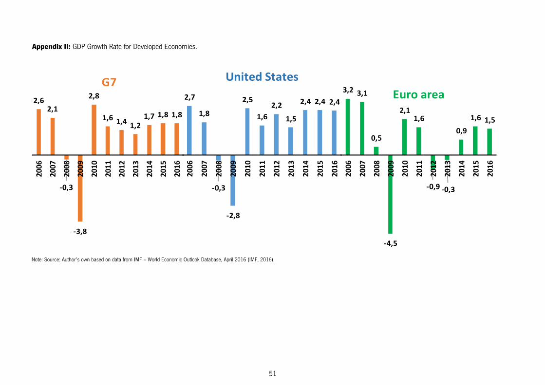
51

Appendix II: GDP Growth Rate for Developed Economies.

2,6

2,1

-0,3

-3,8

2,8

1,61,4

1,2

1,7 1,8 1,8

20

06

20

07

20

08

20

09

20

10

20

11

20

12

20

13

20

14

20

15

20

16

G73,2 3,1

0,5

-4,5

2,11,6

-0,9 -0,3

0,9

1,6 1,5

20

06

20

07

20

08

20

09

20

10

20

11

20

12

20

13

20

14

20

15

20

16

Euro area 2,7

1,8

-0,3

-2,8

2,5

1,6

2,2

1,5

2,4 2,4 2,4

20

06

20

07

20

08

20

09

20

10

20

11

20

12

20

13

20

14

20

15

20

16

United States

Note: Source: Author’s own based on data from IMF – World Economic Outlook Database, April 2016 (IMF, 2016).

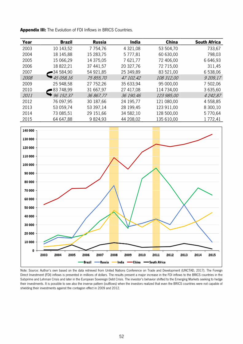
52

Appendix III: The Evolution of FDI Inflows in BRICS Countries.

Year Brazil Russia India China South Africa 2003 10 143,52 7 754,76 4 321,08 53 504,70 733,67

2004 18 145,88 15 283,75 5 777,81 60 630,00 798,03

2005 15 066,29 14 375,05 7 621,77 72 406,00 6 646,93

2006 18 822,21 37 441,57 20 327,76 72 715,00 311,45

2007 34 584,90 54 921,85 25 349,89 83 521,00 6 538,06

2008 45 058,16 75 855,70 47 102,42 108 312,00 9 209,17 2009 25 948,58 27 752,26 35 633,94 95 000,00 7 502,06

2010 83 748,99 31 667,97 27 417,08 114 734,00 3 635,60

2011 96 152,37 36 867,77 36 190,46 123 985,00 4 242,87 2012 76 097,95 30 187,66 24 195,77 121 080,00 4 558,85

2013 53 059,74 53 397,14 28 199,45 123 911,00 8 300,10

2014 73 085,51 29 151,66 34 582,10 128 500,00 5 770,64

2015 64 647,88 9 824,93 44 208,02 135 610,00 1 772,41

Note: Source: Author’s own based on the data retrieved from United Nations Conference on Trade and Development (UNCTAD, 2017). The Foreign

Direct Investment (FDI) inflows is presented in millions of dollars. The results present a major increase in the FDI inflows to the BRICS countries in the

Subprime and Lehman Crisis and later in the European Sovereign Debt Crisis. The investor’s behavior shifted to the Emerging Markets seeking to hedge

their investments. It is possible to see also the inverse pattern (outflows) when the investors realized that even the BRICS countries were not capable of

shielding their investments against the contagion effect in 2009 and 2012.

53

Appendix A: BRICS and USA Stock Markets – Individual Log-Level Representation.

Note: Source: Author’s own. Using EVIEWS 9.0 program.

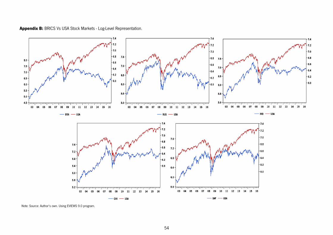
54

Note: Source: Author’s own. Using EVIEWS 9.0 program.

Appendix B: BRICS Vs USA Stock Markets - Log-Level Representation.

55

Appendix C: BRICS and USA Stock Markets - Percentage Daily Returns.

Note: Source: Author’s own. Using EVIEWS 9.0 program.

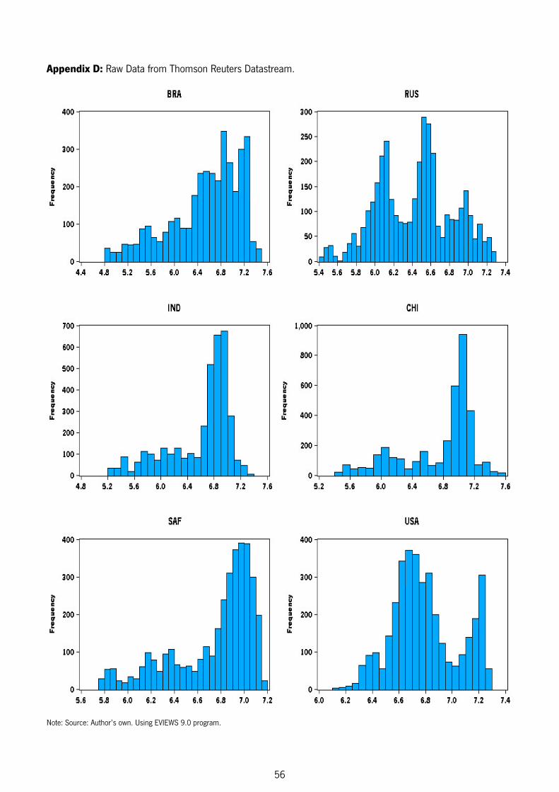
56

Appendix D: Raw Data from Thomson Reuters Datastream.

Note: Source: Author’s own. Using EVIEWS 9.0 program.

57

Appendix E: Data Transformation in Log-Level.

Eq. 1

Formula: � = [l�� � − l�� � − × ] = [l�� ����− × ]

Note: Source: Author’s own. Using EVIEWS 9.0 program. Logged values are taking to reduce heteroskedasticity present in the data (Singh & Kaur, 2016).