Fluid model equations for the tokamak plasma edgearies.ucsd.edu/najmabadi/PAPER/A1-026-91-PF-Vold.pdf · Fluid model equations for the tokamak plasma edge E. L. Void,@ F. Najmabadi,

Fluid model equations for the tokamak plasma edge E. L. Void,@ F. Najmabadi, and R. W. Conn Institute of Plasma and Fusion Research, University of Cai.$oarnia, Los Angeles, Caiifornia 90024

(Received 11 February 1991; accepted 14 June 1991)

Increasing evidence that the edge plasma plays a crucial role in global tokamak continement motivates this study of two-dimensional (2-D) (0,~) computational models of fluid transport in the edge plasma region. Fluid plasma equations, boundary conditions, and a coupled neutral-plasma model are developed assuming toroidal symmetry. A plasma potential equation~is presented for consistent drift flow solution in the nonambipolar case, Simplified plasma equations are implemented in a 2-D computational model. Results show large poloidal flux dominated by drift flow near the separatrix and parallel flow near the ,tokamak divertor target. Simultaneously large polo&l gradients in plasma potential and elestric fields are seen. These may play a role in driving observed turbulent fluctuations in the edge plasma.

I. INTRODUCTION The edge region, or “boundary layer,” of a magnetically

confined high-temperature plasma is observed experimentally to be complex and dynamic, Significant fluctuation levels in the plasma density and plasma potential have been related theoretically and experimentally to the anomalous transport observed in tokamak devices.’ Electrostatic oscillations are found to be maximum in this edge region.273 Core plasma density limits4 and improved global confinement in the H mode516 have been related to the physics of the edge plasma, although the mechanisms are not well understood. Additionally, neutral particle and plasma recycling in the edge must be controlled to maintain acceptably low plasma temperatures at the walls and to minimize sputtering and erosion losses. The behavior of the edge plasma is critical in designing particle and power exhaust systems for the power leveis expected in fusion reactors.

The plasma sheath formed at the walls accelerates plasma ions to the sound speed, and acts as a sink for momentum in the plasma. This must be balanced by the momentum efflux from the core plasma. The interface between the core and the edge plasma region is where a boundary condition is established for the core plasma. No computational codes ex- ist that self-consistently couple transport in these two regions.

A goal of this paper is to develop a model that can be implemented computationally in a stepwise fashion while improving approximations to drift flows and nonambipolarity with each step. The aim is to obtain a fully self-consistent calculation in the edge region. An important consideration is coupling these equations with the core plasma region at the core-edge interface.

A set of plasma fluid transport equations is developed and their application to the edge plasma region is described. Simplifying assumptions to obtain a computationally manageable form are explicitly delineated. We first briefly review existing models of the edge region, focusing on two-dimen-

‘) Present address: Applied Theoretical Physics Division, Los Alamos Na- tional Laboratory, Group X-4, MS F664, Los Alamos, New Mexico 87545.

sional (2-D) fluid models and then develop equations for a toroidally symmetric device, including plasma drifts. Non- ambipolarity and a plasma potential equation are discussed. The classical and anomalous viscosity tensor elements are compared, Ambipolarity and additional simplifications to the ff uid model are discussed for numerical implementation in the EPIC code.“’

We turn next to the important role of recycling of the plasma and neutral particle transport, which necessitates a self-consistently coupled plasma-neutral model. A neutral fluid diffusion approximation is used, which has been discussed more extensively in a separate paper.’ Boundary conditions are reviewed with emphasis on the cor+scrapeoff layer (SOL) interface boundary condition. The simplified plasma equations are applied to a tokamak divertor plasma and the results are discussed with an emphasis on the poloidal flow, the plasma potential, and the potential gradient electric fields. Implications of the results on transport are discussed.

II. TWO-DIMENSIC~NAL EDGE PLASMA FLUID MODELS

Plasma solutions to 2-D steady-state computational fluid models can be compared to the experimentally observed “steady-state” or time-averaged solutions in the plasma edge. Other approaches such as plasma simulations’O** ’ or drift wave models’2*‘3 attempt to simulate the fluctuation behavior or a particular instability in the edge plasma and are not covered hese.

Several groups have reported two-dimensional (2-D) steady-state results in the plasma fluid edge region.7v’b29 These codes are summarized briefly in Table I. The equations vary in format: but are all variations on the plasma fluid equations of Braginskii.30 The continuity equation is solved for plasma density, the momentum equation is solved for the parallel velocity component, and one or two energy equations are solved for temperature ( Tor Ti and T, ) . The radial transport is assumed to be anomalous and generally diffusive. Transport in the flux surface is assumed to be dominated by parallel flow.

3132 Phys. Fluids B 3 (1 l)? November 1991 0899-8221 f91 /113132-21$02.00 c!J 1991 American institute of Physics 3132

Downloaded 01 Sep 2002 to 132.239.190.78. Redistribution subject to AIP license or copyright, see http://ojps.aip.org/pop/popcr.jsp

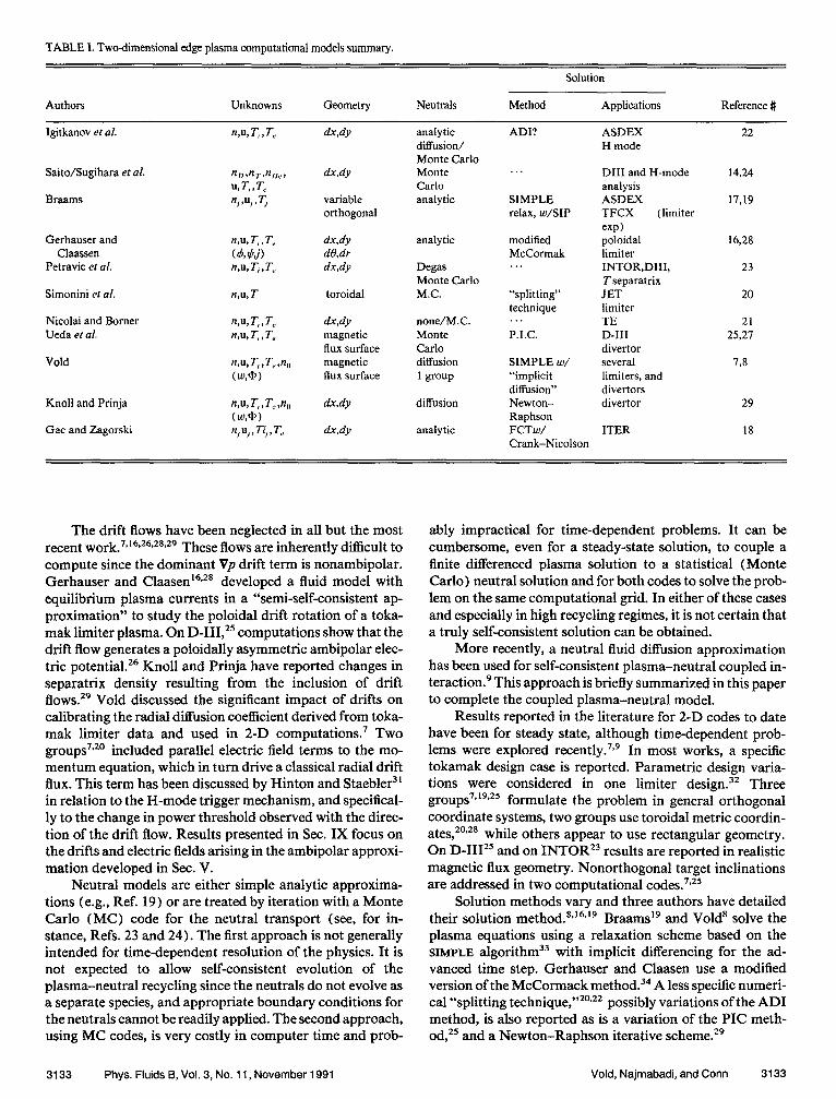
TABLE I. Two-dimensional edge plasma computational models summary.

Authors Unknowns Geometry Neutrals Method

Solution

Applications Reference #

Igitkanov et al. n,u, T, , T, dx,&

Saito/Sugihara et al.

Braams

Gerhauser and Claassen

Petravic et al.

Simonini et al.

Nicolai and Bomer Ueda et al.

Vold

Knoll and Prinja

Gac and Zagonki

nDdwh u,T,Te n,,u,,T,

n,u,T,,T, c4,w n,u, T, , T,

n,u, T

n,u, T, , T, n,u, T, , T,

n,u, T, , T, ,n, (w,Q)

n,u, T,,T,,n,, (w,Q) n,u,,Ti,,T,

dx,dy

variable orthogonal

dx,& dt’,dr dx,dy

toroidal

dxdy magnetic flux surface magnetic flux surface

d.W

d-v+

analytic diffusion/ Monte Carlo Monte Carlo analytic

analytic

Degas Monte Carlo M.C.

none/M.C. Monte Carlo diffusion 1 group

diffusion

analytic

ADI?

. . .

SIMPLE relax, w/SIP

modified McCormak . . .

“splitting” technique . . . P.I.C.

SIMPLE w/ “implicit diffusion” Newton- Raphson FCTw/ Crank-Nicolson

ASDEX H mode

DIII and H-mode analysis ASDEX TFCX (limiter exp) poloidal limiter INTOR,DIII, T separatrix JET limiter TE D-III divertor several limiters, and divertors divertor

14,24

17,19

16,28

23

20

21 25,27

73

29

ITER 18

22

The drift flows have been neglected in all but the most recent work.7~‘6~26~**~29 These flows are inherently difficult to compute since the dominant Vp drift term is nonambipolar. Gerhauser and Claasen’6*28 developed a fluid model with equilibrium plasma currents in a “semi-self-consistent approximation” to study the poloidal drift rotation of a tokamak limiter plasma. On D-III,25 computations show that the drift flow generates a poloidally asymmetric ambipolar electric potential.26 Knoll and Prinja have reported changes in separatrix density resulting from the inclusion of drift flow~.~’ Vold discussed the significant impact of drifts on calibrating the radial diffusion coefficient derived from tokamak limiter data and used in 2-D computations.’ Two groups’,” included parallel electric field terms to the momentum equation, which in turn drive a classical radial drift flux. This term has been discussed by Hinton and Staebler3’ in relation to the H-mode trigger mechanism, and specifically to the change in power threshold observed with the direction of the drift flow. Results presented in Sec. IX focus on the drifts and electric fields arising in the ambipolar approximation developed in Sec. V.

ably impractical for time-dependent problems. It can be cumbersome, even for a steady-state solution, to couple a finite differenced plasma solution to a statistical (Monte Carlo) neutral solution and for both codes to solve the problem on the same computational grid. In either of these cases and especially in high recycling regimes, it is not certain that a truly self-consistent solution can be obtained.

More recently, a neutral fluid diffusion approximation has been used for self-consistent plasma-neutral coupled interaction.’ This approach is briefly summarized in this paper to complete the coupled plasma-neutral model.

Neutral models are either simple analytic approximations (e.g., Ref. 19) or are treated by iteration with a Monte Carlo (MC) code for the neutral transport (see, for instance, Refs. 23 and 24). The first approach is not generally intended for time-dependent resolution of the physics. It is not expected to allow self-consistent evolution of the plasma-neutral recycling since the neutrals do not evolve as a separate species, and appropriate boundary conditions for the neutrals cannot be readily applied. The second approach, using MC codes, is very costly in computer time and prob-

Results reported in the literature for 2-D codes to date have been for steady state, although time-dependent problems were explored recently.7F9 In most works, a specific tokamak design case is reported. Parametric design variations were considered in one limiter design.32 Three groups7*19*25 formulate the problem in general orthogonal coordinate systems, two groups use toroidal metric coordinates,20’28 while others appear to use rectangular geometry. On D-III25 and on INTOR23 results are reported in realistic magnetic flux geometry. Nonorthogonal target inclinations are addressed in two computational codes.7,2s

Solution methods vary and three authors have detailed their solution method.8~16*‘9 Braams” and Void’ solve the plasma equations using a relaxation scheme based on the SIMPLE algorithm33 with implicit differencing for the ad- vanced time step. Gerhauser and Claasen use a modified version of the McCormack method.34 A less specific numerical “splitting technique,“20’22 possibly variations of the AD1 method, is also reported as is a variation of the PIC method,25 and a Newton-Raphson iterative scheme.29

3133 Phys. Fluids B, Vol. 3, No. 11, November 1991 Vold, Najmabadi, and Conn 3133


Summarizing, the present code is unique in that it includes simultaneously several key features: coupled plasma- neutral fluids, realistic magnetic flux surfaces including divertor geometries, and determination of the drift flux and ambipolar eIectric fields outside the separatrix. The finite difference implementation and time-dependent residual cor- rection7.* assure accurate convergence of the coupled plasma-neutral model in the highly nonlinear regime of high- density divertor recycling. This has allowed several time-dependent problems to be examined.‘g9 In common with other edge plasma codes, we assume an anomalous diffusive flux dominates the radial transport, and that parallel flow dominates the poloidal edge plasma flux. Implications of these assumptions are discussed throughout this paper, and primarily in Sec. V.

111. MODEL EQUATIONS Transport equations are presented to describe the plas-

ma in the fluid approximation, appropriate for the low beta plasma edge region of a tokamak or similar magnetic confinement device. The detail is important to understand the simplifying assumptions discussed in Sec. V and to support the longer term goal of self-consistent fluid momentum computations, as discussed throughout. The plasma treatment is based on that of Braginskii,30 and discussed by Miyamoto.35 Metric forms with toroidal symmetry are developed in Sec. IV.

An orthogonal coordinate system (s,r,q) is aligned with the plasma flow pathlength ds along the magnetic field axis s with B = B,s. The “radial” direction r is normal to the magnetic flux surfaces $ with increasing values directed outward. The third orthogonal direction is denoted by q where q = r Xs, the fluid drift direction. The corresponding components to be derived for the fluid velocity u are written as

u=us$vr+wq;

thus u = u*B, u = WV+, and w = u*(V+xB), and total fluid speeds are related as,

V2=u2+3+d. The s,r,q coordinates are shown in Fig. 1. The figure relates these coordinates to the toroidal geometry coordinates, as shown in Figs. 1 and 2.

A. The plasma fluid equations The starting point is the Boltzmann kinetic equation for

the plasma species distribution function, f( t,x,v), subject to the effects of collisions and to the body force F due to statisti- cally averaged E and B fields. The fluid model is based on averaged distribution quantities arising from the Boltzmann equation in the integral velocity moments. This defines the density n and fluid velocity u, respectively

n = J

f(f,r,v)du, (1)

u = -!- v$+( t,r,v)dv. n J (2)

A general temperature T is defined with the total velocity,

FIG. 1. Coordinate systems: relationship between the magnetic geometry coordinates s,r,q and the toroidal coordinates B,r,4.

written as the sum of the fluid average and a fluctuating component, v = u -I- v’, or

T = -!- n J y(v - u)2f(t,r,v)du (3)

= (m/3)((v - uy) = (m/3)(v’2). (4) With these definitions the zeroth, first, and second mo-

ments of the Boltzmann transport equation give the general form for each plasma species as

continuity: s+V+nr) = J C, du=S,(n,); (5) momentum:

9 + V+?zn(~w))

=ne(E+uxB) + [C,mvdv+ fC,,mvdu (6)

energy: J J

a f (m/2>M) 1 at + v.(F nwv))

= neE*u +- J

C,‘, ; rrn2 dv

+ c+u2dv-P,,. J r

e-'----- *'

. . ...\

#' 'a : :

c2

i

c >

r* =

: : ', : , '. *. *..__.c--

/

C.L.

(7)

FIG. 2. Poloidal cross section showing poloidal components of flux with contributions from the rlarallel and drift flux terms. The magnetic field weighting factors for each flux follow directly from Fig. I.

3134 Phys. Fluids B, Vol. 3, No. 11, November 1991 Void, Najmabadi, and Conn 3134


Collisions with neutrals are represented by C, and electron-ion collisions by Cei. An ion-ion collision integral can be added for multicomponent plasmas. The term, Prad , is a radiation power loss due to atomic processes and is significant only in the electron energy equation.

These equations are exact but solutions require additional assumptions regarding the physics to express the instantaneous velocity Y as a function of the fluid-averaged velocity u. This assumed constitutive relationship is likely different in form for electrons and ions, so that v, = f, ( u1 ,u, ) and vi =A (II, ,I+ ) . Various simple assumptions regarding these functions, & and f,, offer a point of departure for future studies to solve the coupled momentum equations directly.

In the momentum equation (6)) it is averaged velocity that remains in the Lorentz force term, uXB, but the instantaneous velocities in the kinetic flux tensor, (mn (vv) ) and in the collision integrals. The flux tensor in the momentum equation is conventionally simplified by assuming that the instantaneous velocity v is the linear sum of the average velocity u and the random component v’. This contributes to a fluid convective term, mnuu, and the kinetic pressure tensor term, P = mn(v’v’), as

mn(w) =mn((u+v’)(u+v’))

= mnuu + mn(v’v’). (8)

Here the usual assumption is made that (uv’) = 0, which is exact if the mean and fluctuating components of flow can realistically be linearly separated. Conversely, once we have made this assumption we have lost a nonlinear coupling of the mean fluctuating fluids implied in (uv’) . If this nonlinear coupling of mean and fluctuating components is physically significant (as is evidenced in the plasma edge region) then one needs a “turbulent” model to reintroduce this nonlinearity into the system.

The components of the kinetic pressure tensor, Pap, are composed of the diagonal scalar pressure and the off-diagonal “viscosity” tensor, II,. Moment terms arising in the energy (or second moment equation) are evaluated by Bra- ginskii and the dominant components are put in the classic form for anisotropic heat conduction:

q= --,I v,,T-KK, V,T+K,~XV,T, (9) where the conductivity tensor coefficients K are evaluated using a linear expansion of the distribution function about the Maxwellian-averaged distribution. The parallel conduction is of order of the unmagnetized plasma conduction, K,, ~K,,~nTTr/m, while K, ZK~(WQ) and K~ SKY*.

The heat conduction in the direction, s XVT, is smaller than the parallel conduction by the classical expansion factor, (or) - I = (p,/;l) (where the gyrofrequency times the collision time equals the Larmor radius over the collision mean-free path). This heat conduction term is thus proportional to K x =: n T /B, a “Bohm-like” diffusivity of heat discussed in Sec. V C. A third term in qe for the electron heat flux arises from the thermal force discussed by Braginskii30 and Miyamoto.35 This term is written as 4 c.11 = - O.‘llnuV,, T,.

The results of the Braginskii analysis to evaluate the momentum and energy flux tensors needed to close the first three moments of the general Boltzmann transport equation are a set of transport equations applicable to each plasma species in terms of its average fluid velocity u. These equations can be written as

continuity: Z!!- + V*( nu) = S, (no>; 1 at (10)

momentum:

@$. + V*(mnuu - v:Vu) + Vp

= ne(E + uXB) + R + F, + S, (no);

energy: a [pT+ (m/2)nV*]

at

(11)

nT+FnV2)u-K:VT]

=neE*u+R*u+Q+& +F,*u+P,,, +S,(n,), (12)

where the neutral collision terms for each moment are, respectively, S, (no ) , SP (no>, S, (no>, and Fg is a general body force. The forces due to electron-ion collisions are in the term R, QviS is the viscous heating, and the term Q is the thermal energy exchange in collisions. The collision force term has a friction component proportional to the relative velocity u, - uj, and the thermal term

R = f (m,n,/7,)[0.51(u,--i)ll + (u, --ui),] - 0.71n, V,, Te,

neglecting terms of order l/o, 7,. (13)

It is worth considering the validity of the plasma fluid equations as limited by the expansion procedure used by Braginskii to evaluate the flux tensors. This procedure as- sumes that the zeroth-order distribution is the equilibrium distribution, the Maxwellian, denoted byfo. A linear perturbation in the distribution function is assumed, f =f” +f’, and substituted into the Boltzmann equation, with linear products in the collision terms retained. The set of linear equations for the perturbation quantities are solved and the results are expressed in terms of the viscosity and conductivity coefficients in generalized viscosity and conductivity matrices, respectively.

Two important limitations are that nonlinear terms in the expansion are not retained, and that perturbations from the Maxwellian equilibrium due to electrostatic fluctuations are not considered. The exact momentum equation (6) shows that the flux tensor is balanced by the “fluctuations” in v in the collision operator, as in ordinary fluids, and by the E’ fluctuations linked by the EXB velocity fluctuations, v’ = (E’ X B ) /IS. Experimental evidence suggests that in the plasma edge neEz n’eE= neE ’ % C, where C is the collision integral in Eq. (6). The electric field terms are larger than the collision term and deserve an explicit role in defining the kinetic pressure tensor.

At frequencies well below the collision frequency, the distribution is expected to be maintained nearly Maxwellian, even in the presence of electrostatic fluctuations. In this case,



the term E in Eqs, ( 11) and ( 12 ) is accurate and an expansion using E = E” + E’ is not appropriate. One might coun- terargue that for large wave number k or small wavelength disturbances, less than the collision mean-free path, R,,, the “Maxwellianization” due to the collisions is not possible and so E’(k -‘<A,, ) is possible, even at frequencies below the collision frequency.

Discrepancies between observed and classical (Bragins- kii) cross-field transport suggests that collisions are not the dominant process for momentum diffusion. A self-consistent fluid approximation for momentum diffusion by electrostatic oscillations is needed. The nonlinearity of this problem has precluded analytic solutions but numerical computations of a fluid model with appropriately defined momentum diffusivity may be possible. “Appropriately defined” implies that the time-dependent electrostatic collec- tive oscillations responsible for “anomalous” transport are taken into account in the momentum diffusivity definition assumed to close the momentum flux tensor. Specifically, this will require significant off-diagonal “viscosity” terms, where II,(a#/3) =J(E), or alternatively vi =f;:(ui,u,) and U, = fC ( ui,u, ). We do not elaborate further on this point in this paper.

6. Single flufd equations and Ohm’s law The previous equations apply to each plasma species.

For a single ion species, or amass-averaged ion to represent a mixture, there is a fluid velocity ui for the ions and a velocity u, for the electrons. Quasineutrality is assumed, so n, z n i. It is convenient to work with a single mass-averaged velocity for the plasma: U = (m,tt, -I- MjUi)/(m, + Mj) = tli + (m,/Mj)11,ZUi.

(14) The electron velocity can then be expressed in terms of the ion or plasma velocity ui and a difference velocity or plasma current: j = ne(u, - u, ), so that u, = ui - j/ne.

The single fluid momentum equation follows by sum- ming the electron and ion momentum equations and neglecting terms of order m,/M,. The result is a(mnu) - + W(mnuu - V:Vu) + Vp at

=jXB+Spi(no) +$,Gd, (15) where neutral momentum sources from both the ion and electron equations are included, The electron contribution S,, (n,) can be shown to be a small term. Viscosity is that of the ions.

An equation for the current j is derived from a mass- weighted difference of the electron and ion momentum equations, giving rise to the generalized Ohm’s law. Viscous terms are neglected because II, 4 I& and Ohm’s law includes the small product m,l&. The resulting Ohm’s law can be written as

3 $f + V*(uj -l-b) - V* [

P ( >1 z

. =E+uxB---- ~ jXB + VP,

0 en en

f (0.71/e)Vll T, f dP(n,), where the neutral interaction term is

(16)

dP(no) = (

tmesSPi(nOl -Mj’SP,(BO)] ~ hijet )*

(17)

The terms on the left side of Eq. ( 16) are often neglected. This is valid for l;he first term at frequencies well below the plasma frequency. The second and third terms in the bracket arise from the convective terms in the momentum equations. Neglecting these terms may be a poor assumption when nonambipolar currents are large and nonlinearities be- come significant in the V-f term, Hasegawa and MimaL2 note that their edge turbulence model depends critically upon the convective derivative of the polarization drift term. That term in their drift model is related to the convective current terms in the present single-fluid model, so these terms may be required in a model that includes drift wave turbulence,

Neglecting the b,racketed terms, the generalized Ohm’s law becomes

. v(zl+Q--- jXB

o- en VP, =uxB+-- + 0.71

-V,,Te+dP(n,L (18) ne e where we assumed that E is noninductive and thus derived as E = - V@. If the Hall current term, (j X B) /en, is neglected in this form, the velocity in the Ohm’s law becomes that of the electron fluid and not that of the plasma, so this term must be included if cross-field current is nonzero as is observed experimentahy in the edge region.36 The usual assumption in many magnetohydrodynamic ( MHD ) models to drop the Hall current term is a poor assumption in the edge plasma, where diamagnetic currents dominate.

C. Plasma potential equation The equation for continuity of plasma charge is

where pC = qni - en,, and j = qnui - enu,. The current source Sj can result from plasma-neutral interactions or from imposed sources, however, it is generally assumed that Sj = 0. Quasineutrality implies pc ~0, and the above equation is

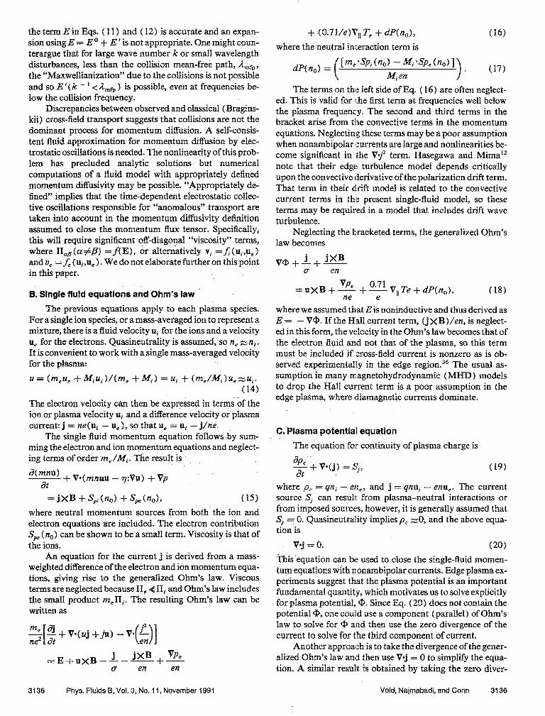
v-j = 0. (20) This equation can be used to close the single-fluid momentum equations with nonambipolar currents. Edge plasma experiments suggest that the plasma potential is an impartant fundamental quantity, which motivates us to solve explicitly for plasma potential, @. Since Eq. (20) does not contain the potential @, one could use a component (parallel) of Ohm’s law to solve for @ and then use the zero divergence of the ‘current to solve for the third component of current.

Another approach is to take the divergence of the generalized Ohm’s law and then use V-j = 0 to simplify the equation. A similar result is obtained by taking the zero diver-



gence of current and simply substituting from the Ohm’s law component equations into this equation for the current terms. The result is an elliptic equation for +, a “generalized quasineutral Poisson equation,” which can be used to complete the set of nonambipolar plasma fluid equations. This potential equation is

VP, uxB + - ne

+ 0.71 F +dP(n,) -= . ne >I

(21) Further manipulation can eliminate current j from the rhs. One motivation for casting the equation in this form is that it is computationally convenient. For a given source term on the right-hand side, it can always be written in a diagonally dominant finite differenced form, which produces an impli- citly stable system of equations for a.

The boundary conditions for this equation specify the potential at the plasma sheath formed at the divertor or limiter wall. The boundary condition at the edge-core interface is more difficult (or uncertain) to specify. One solution is to extend the evaluation of the potential equation into the core where a symmetry or zero gradient boundary condition would apply at the core center. Solving for <P in the core entails solving a set of MHD equations, however, with the currents and B fields solved self-consistently. An induced emf term could be added into the brackets on the rhs of the potential equation (21). In an induction-driven tokamak, this adds an induced toroidal component of the electric field, while the steady-state potential gradient field has only poloi- da1 and radial components in a toroidally symmetric device. One can further modify the source terms if strong sources of j or u are imposed by additional external means such as neutral beam injection. In the present computations, the simplifications discussed in Sec. V make the core-edge plasma interface boundary conditions irrelevant, and thus not fully self-consistent.

The importance of including a plasma potential equation is established in several previous studies. Combining nonlinear equations for the plasma density and plasma potential with the assumed flux (velocity component) terms has produced time-dependent simulations with chaotic or “turbulent” solutions. 12*13 Coupling the plasma density and the potential with consistently evolved momentum equations subject to the plasma edge region boundary conditions has not been reported. A coupled plasma density and potential solver in the limit of weakly ionized plasma has proven successful in predicting experimental simulations of the steady-state edge plasma. 37 The fluctuating potential and steady-state potential profiles may be related in the H-mode improved confinement.“a

D. Energy equations Using the single fluid velocity u, the ion energy equation

can now be written as

a pzTi + (m/mlYZ] dt

+ v- K +1; +~nV’)U-ui:VTi]

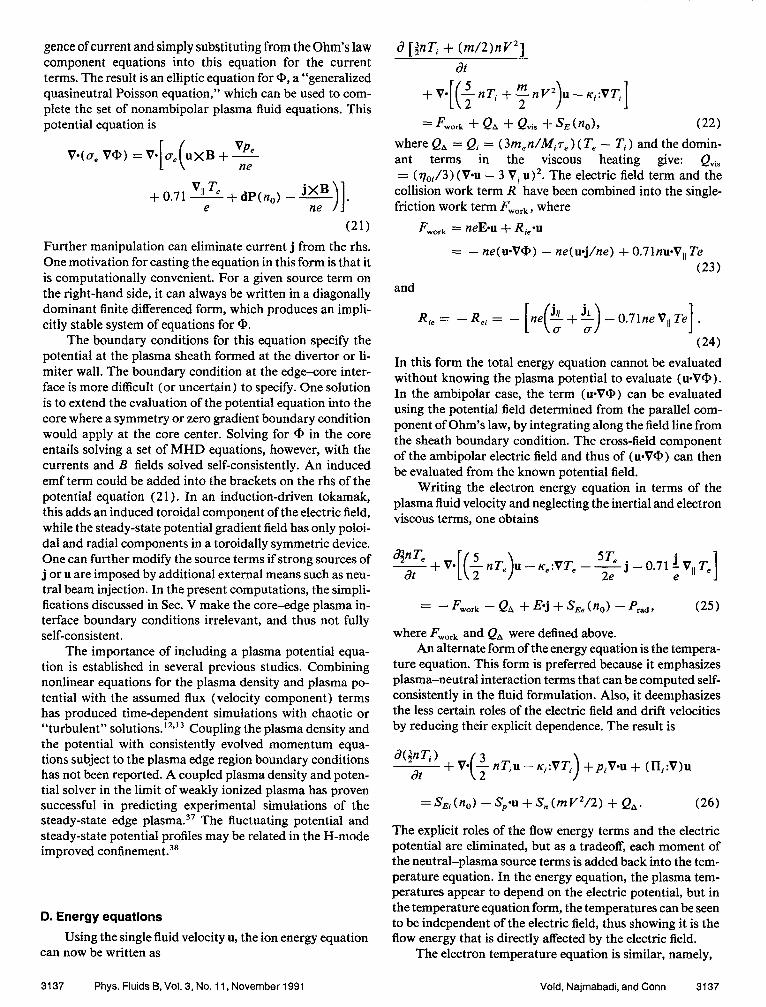
= Fwork + QA + Qvis + SEtno), (22) where QA = Qj = (3m,n/M,r, ) ( T, - Ti ) and the dominant terms in the viscous heating give: Qvis = (%/3) (Vu - 3 V,,u)*. The electric field term and the

collision work term R have been combined into the single- friction work term Fwork , where

F work = neE*u + R,*u =- ne(u.V@) - ne( u.j/ne) + 0.7lnu*V,, Te

(23) and

R,= -Rei= -[ne($+$)-0.7lneV,,Te].

(24) In this form the total energy equation cannot be evaluated without knowing the plasma potential to evaluate (u-V@). In the ambipolar case, the term (u*V@) can be evaluated using the potential field determined from the parallel component of Ohm’s law, by integrating along the field line from the sheath boundary condition. The cross-field component of the ambipolar electric field and thus of (u-V@) can then be evaluated from the known potential field.

Writing the electron energy equation in terms of the plasma fluid velocity and neglecting the inertial and electron viscous terms, one obtains

u - u,:VT, - ST, . --J-0.71iV T, e ” 1

= - Fwork -QA +&i+S,,(n,) -Prad, (25)

where Fwork and Q, were defined above. An alternate form of the energy equation is the tempera-

ture equation. This form is preferred because it emphasizes plasma-neutral interaction terms that can be computed self- consistently in the fluid formulation. Also, it deemphasizes the less certain roles of the electric field and drift velocities by reducing their explicit dependence. The result is

a($Ti 1 - + dt v* $ nT+ - Ki:VTi >

+piV*u + (I&:V)u

=SEi(no) -Sp*u+S,(mV2/2) +Q,. (26)

The explicit roles of the flow energy terms and the electric potential are eliminated, but as a tradeoff, each moment of the neutral-plasma source terms is added back into the temperature equation. In the energy equation, the plasma temperatures appear to depend on the electric potential, but in the temperature equation form, the temperatures can be seen to be independent of the electric field, thus showing it is the flow energy that is directly affected by the electric field.

The electron temperature equation is similar, namely,



+,,v*(=$) + crI:v,*(~)

= S,(n,) - S,* 5 ( > ne

mV* +s,------ 2

QA +R, ‘-Prd* ne

The electron viscosity terms are small and henceforth neglected. In ambipolar flow, the electron temperature equation simplifies to a form similar to that for the ion temperature. In nonambipolar flow, T, depends on the currents and thus requires a coupled solution of the continuity, momentum equations, Ohm’s laws, T, , Ti and one additional equation to close the set, V-j = 0.

A.1

This completes the general formulation of the plasma edge fluid transport equations, a formidable set of ten plasma equations (plus equations for the neutrals). Closure requires evaluation of the viscosity and conductivity tensors, which are assumed to involve approximations to anomalous cross- fieldtransport. We return to discuss the simplifying assumptions needed to close the plasma equation set in Sec. V.

IV. METRIC FORMULATlON OF THE EDGE PLASMA EQUATIONS

0.4 0.6 x (4"

1.0

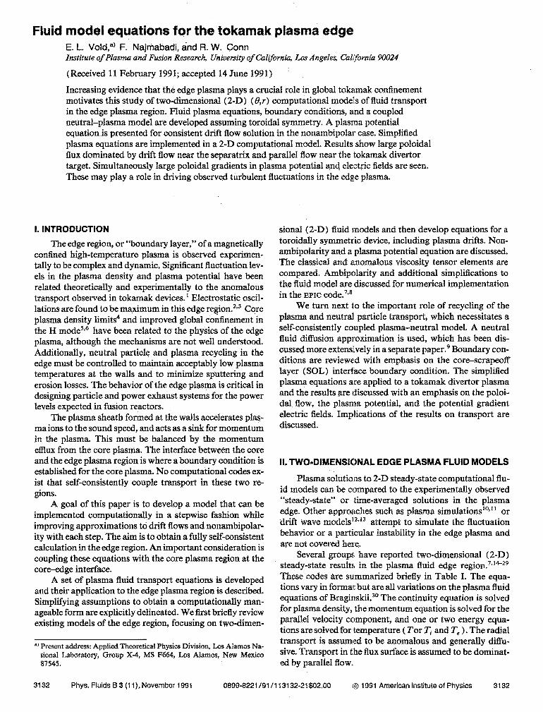
Toroidal symmetry is a realistic assumption in many tokamak devices. The assumption of toroidul symmetry allows us to speclfi the complete 3-D problem with only two

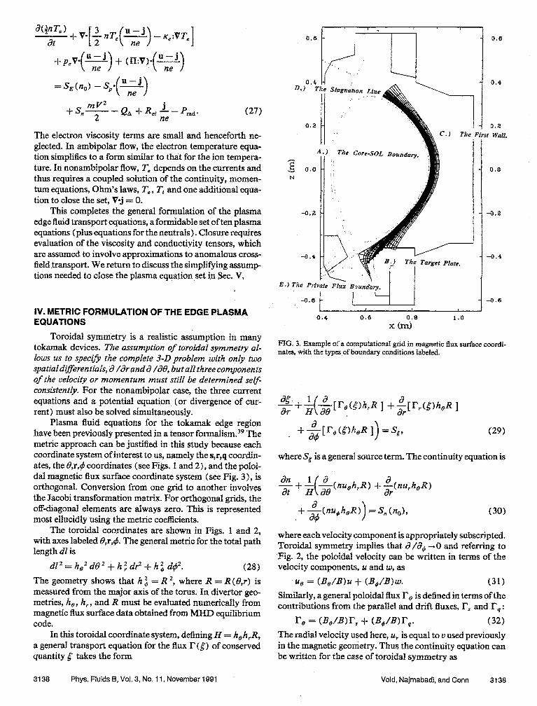
FIG. 3. Example of a computational grid in magnetic flux surface coordi- natea, with the types of boundary conditions labeled.

spatialdifferentials, d /ar and d /a@, but alf three components of the velocity or momentum must still be determined self- consistently. For the nonambipolar case, the three current equations and a potential equation (or divergence of current) must also be solved simultaneously.

%+- A(;[ re(W,R ] + -$ r,(iW@ ]

Plasma fluid equations for the tokamak edge region have been previously presented in a tensor formalism.39 The metric approach can be justified in this study because each

+-$[~,G)~~,R ])=S6, (29)

coordinate system of interest to us, namely the s,r,q coordinates, the e,r,+ coordinates f see Figs, 1 and 2), and the poloi-

where S, is a general source term. The continuity equation is

dal magnetic flux surface coordinate system (see Fig. 3)) is orthogonal, Conversion from one grid to another involves

i a -W&R) the Jacobi transformation matrix. For orthogonal grids, the

$+- ( H at9 t $(ns,h,R)

off-diagonal elements are always zero. This is represented most ellucidly using the metric coefficients. + a4

-QnuJz,d!) >

= S, (no), (30)

The toroidal coordinates are shown in Figs. 1 and 2, with axes labeled B,r,#. The general metric for the total path length dl is

dl*=he*dB*+h;d~+h~d~*. (28) The geometry shows that h $ = R *, where R = R (6,r) is measured from the major axis of the torus. In divertor geometries, he, h, , and R must be evaluated numerically from magnetic flux surface data obtained from MHD equilibrium code.

In this toroidal coordinate system, defining H = h&R, a general transport equation for the flux E’ (4) of conserved quantity 4 takes the form

where each velocity component is appropriately subscripted. Toroidal symmetry implies that 8 /a, + 0 and referring to Pig. 2, the poloidal velocity can be written in terms of the velocity components, u and w, as

zig = (B*/B)u + (B&3)w. (31) Similarly, a general poloidal flux I’, is defined in terms of the contributions from the parallel and drift fluxes, P, and P4 :

re = CB,mr, + (B,mr,. (32) The radial velocity used here, U, is equal to v used previously in the magnetic geometry. Thus the continuity equation can be written for the case of toroidal symmetry as



~+~{~[nh,R(~‘+~w)] + -+,R) = S,(n,). I

Neglecting the drift velocity w is of questionable validity, ‘J’ but its poloidal derivative, as in Eq. (33)) is expected to be small, except near the target plate. There the poloi- da1 gradient of the parallel velocity is expected to be a larger term, With this caveat, if one neglects the drift velocity as small (w-+0), then

~+~$(nh,R~u)+$~(nuh,R) =S*(no). (34)

This form, often neglecting the metrics, is common in edge plasma modeling. Note that the B field scale factor is within the poloidal gradient operator rather than outside.

The parallel momentum equation is a(mnu) -+v*(r,) +~p=S,(n,)s, at (35)

where ry is the flux of parallel momentum. In the 8,r,# system, this equation becomes

- ~yL?h,R) a(mnu) + 1 a

at

Boa =-- Bheae ’

B-2 - -P + s, (rids, Bh,+

(36)

where the 8 and Q components of the parallel pressure gradient are included. In toroidal symmetry the 4 gradients are again zero. The radial flux is defined as

r, _ r = mnuv f II,, = mnuv - (7j:Vu),, (37) and the poloidal flux of parallel momentum, written in terms of the parallel velocity u is

ruwe = mnu (

Bo 4 -u-+-w B B >

- $@:Vu),

It follows that the parallel momentum equation can be written as a(mnu) -+$$(h’R [mnu(%u+%w) at

4 - !k(,:Vu,, - -+:wsq II + $${h,R [mnuu- (v:Vu),,])

&?a + Bh,dB -p = s, (n,>s. (39)

In writing the divergence of the pressure tensor in this form additional terms that arise from the curvature of the coordinate system are ignored. In a computational solution

based on a control volume formulation, the curvature terms are accounted for in the evaluation of the normal flux to each computational cell surface.

A related simplification is involved when using this form of the pressure gradient term. In Eq. (39)) the metric form correctly reflects the gradient form of the pressure term in Eq. (35). However, the pressure gradient is derived from the trace of the kinetic pressure tensor and the tensor component in general metric form should include the B scale factor inside the differential operator. This point is trivial in the context of the present approximations for the radial and drift flux, but use of the correct metric form will be essential in a self-consistent computational solution of the coupled plasma momentum components.

The classical viscosity in the parallel momentum equation is specified in terms of the toroidal coordinates, for example,

(‘#‘:Vu), = ?/Q(2*V,,u - pl) . (4.0) This is simplified by neglecting terms au/dq and au/&, which lead to cross derivative terms in the divergence operation, so that

(41)

The viscosity component for the radial direction is assumed to be anomalous (as discussed in the following sections) and to have the form

(‘l:Vu) van au “‘Tar’

(42)

Using these viscosity approximations and assuming for the present that the viscosity for parallel momentum in the drift direction is small, ( T,CVU) sq ~0, one obtains the parallel momentum equation:

Bea +- Bh aBP=S,(no)s. e

(43)

If the drift velocity is considered negligible, then w -0 in the above equation.

Derivations similar to that for the parallel momentum equation (43) can be used to obtain the component momentum and current equations in the toroidally symmetric coordinate system( 19,r). The radial component of momentum u is

d(mnv) + 1 a at z ( --&L-&$I +$(T,-.h,R))

+ &P = -j$ + s, (nob, r

3139 Phys. Fluids 6, Vol. 3, No. 11, November 1991 Void, Najmabadi, and Conn 3139


where r,-, = mnvv + II,,

or, with an anomalous viscosity approximation for II,,

r,- 77, a0 --. r = ltZnvv - hr ar (45)

The poloidal flux, in terms of the parallel and drift components of flux, becomes

rem0 =mttv (

$u+ 4 -jyW >

B+ +$II, +pr*.

(46) If the viscosities are classical, one may neglect the viscous terms IIrs and l&. Note, however, that II,, is assumed to contain the significant and anomalous viscosity rjan (as discussed in Sec. IV). One expects tensor symmetry, so that II, = IIn. It is likely then that II, is anomalous as well.

For the drift component of velocity w the momentum equation is

“ma:w) ++&rsh,R) + -$‘,h,R)) + &a

-P = +j,B + S,, (n,>s, Bh (47)

eae

where rp = mnwu + II,, zmnwv

and the poloidal flux of drift direction momentum becomes in terms of the parallel and drift components of flux:

As above, the classical values of I& and II, are small, of order ( wci 7) - I , but anomalous coefficients of viscosity derived from electrostatic fluctuations may be appropriate and may not be negligible.

Ohm’s law involves only gradients and cross products so the form is similar to that used in the s,r,q coordinates, now given in terms of the poloidal and radial gradients. The components are

s component:

-@+A- B,a . Bh,aB *II

= neifae pe + 5 j$$ Te + dP(n,)s; (49)

r component: . a,+J,-k!= -w~+ap,,+dp(~,)~; h,ar aL ni! neh, ar

(50) ij component:

%a jq 0 -----a+ Bh,dB aL+-ne=vB+ ne:haas P, + dP( no) 4. e

(51)

Conservation of charge becomes

-$$-[4R(~Us) +$g))] i-$V@?j.)] =O. (52)

Finally, we turn to the temperature equations in metric form. The ion temperature equation neglecting viscous dissipation, in toroidal symmetry is

(53)

(541

= QA + sEi (noI - uSpj(nof, - uSpi (no), - The electron temperature equation is similar in form for the ambipolar case, ac$nT, 1 - ~~[h,R[~nT~(~u+~w)-(~~+~~)~]}

at + H ae

%)] +$$$[,h,R($&++w)] +-$hgRuj}

The neutral interaction sources S are simplified for the electron case due to the electrons small mass. If nonambipolarity is assumed, then each velocity component in the electron temperature equation must be replaced by the respective component of the electron fluid velocity: u, = u - jhe. The plasma anisotropy in a magnetic fie:ld has made it necessary to work with momentum as a set of three coupled equations for the parallel, magnetic ff ux surface gradient, and drift components.



V. SIMPLIFYING ASSUMPTIONS

The simplifying assumptions used to reduce the general equation to a system that is computationally manageable are summarized. The simplifications allow us to reduce the ten previous unknowns to four coupled plasma variables, n,u,Tj, and T, with a dependent anomalous velocity u,, (n). The neutral density n, is the fifth coupled unknown, self- consistently determined as described in Sec. VII. The ambipolar potential @ and drift velocity w are computed as dependent quantities.

The assumption of toroidal symmetry has been discussed. Additional key assumptions to simplify the plasma fluid equations are the following.

( 1) The flows are ambipolar. (2) The cross-field transport velocity is anomalous and

primarily diffusive in form. This assumption allows us to drop the self-consistent equation for radial velocity and sub- stitute an anomalous flux dominated by the anomalous diffusive term.

(3) The viscosity in the parallel momentum equation is simplified in several ways. The cross-field derivative terms are neglected for computational tractability. The classical cross-field viscosity is replaced with an anomalous viscosity 7, in the tensor component II,,. The anomalous process couples the cross-field transport of particles, momentum, and energy, so O,, _ -van /mn z K,, /nk. Viscous dissipation in the energy equations is neglected, consistent with the large uncertainty in the viscous terms.

(4) The drift velocity is assumed to have a small effect on density, on the parallel momentum and on the temperatures.

(5) The classical parallel conduction for electrons is flux limited.

An additional important assumption is that the characteristic frequencies of phenomena of interest are below the collision frequency of the plasma ions. Thus the ions remain relatively close to a Maxwellian distribution. The experimentally observed electrostatic fluctuations generally held to be responsible for anomalous transport in the edge plasma do not fit this assumption, since the frequency distribution of plasma turbulence UZ lcu’-lo6 Hz) is generally above the ion collision frequency r,- ’ in the plasma edge [e.g., r,- ’ (n = 3 x IO’* m - 3, T = 20 eV) z lo4 Hz]. This implies that a correction for electrostatic fluctuations based on a kinetic model is required before one can solve the coupled fluid momentum equations self-consistently in the edge plasma.

A. Ambipolarity The pressure gradients universally drive drift velocities,

oppositely directed for ions and electrons, so a drift current arises. In a toroidally symmetric device, plasma gradients in the magnetic flux surface are sustained in the poloidal direction and these impose poloidal gradients on the drift current. Gradients in this current combined with the divergence of current equal to zero, implies that some combination of toroidal (or parallel) and radial currents must be nonzero. The ambipolar assumption is that these currents have a small influence upon the transport equations.

In the edge plasma the axial pressure gradients are large owing to the plasma sheath boundary conditions and there the parallel flows can dominate. The parallel pressure bal- ance does not depend upon the current distributions since j enters only in the term j x B. The ambipolar plasma potential is obtained by integrating the parallel Ohm’s law along the field line starting at the target plate, where the boundary condition on the plasma potential is defined from sheath theory to be eQ, =: 3T,. The poloidal projection of the parallel Ohm’s law is used to approximate the ambipolar plasma potential * as

Bd -a= Bh,ae ne:irae pe + y $$ T’ + dP(n,)s.

(55) The equation is accurate, except for the neglect of the parallel current term,j,/o,, . For typical plasma edge values, cl, is large and the current term is small. It was shown elsewhere,*6*28 using a 2-D SOL code that includes an estimate of the nonambipolar currents, that the parallel current is small in a tokamak limiter case. The estimate of the plasma potential from the ambipolar approximation should be reasonably good in the edge region where the field lines termin- ate on the target, and a valid boundary condition can be applied. An exception can occur ifis is driven to large values intentionally, for instance by target plate biasing or other means.4o*4* In trying to extend the simplified model to the closed flux surface region, there is no estimate for the potential boundary condition. Equation (55) cannot be applied there and a plasma potential equation (2 1) should be solved for consistent results.

B. Drift velocities

The Lorentz force, or UXB term, dominates transport in the strongly magnetized plasma. This term couples cross- field velocities and suggests that the poloidal drift velocity is determined to first order by the radial momentum equation. Using the ion momentum equation, and assuming the divergence of the momentum flux can be approximated by the scalar pressure gradient, one obtains

g = ne(E, - wB).

Rearranging this gives the drift velocity w as

(56)

WC Ja@ I lapi ^ B-‘. 1 \ dr nedr/

This drift estimate should prove reasonably accurate in the SOL region where the field lines end on the target. At minor radii less than the tangency/separatrix radius, where the estimate of plasma potential is uncertain, the drift velocity from Eq. (57) is similarly uncertain. A self-consistent drift solution requires solving coupled equations for the drift velocity and the plasma potential.

The assumption that we may neglect the drift velocity in the continuity equation is valid throughout the SOL regions where the parallel flow dominates, especially near the target. The assumption is less valid along the separatrix/tangency line and farther “upstream” away from the target, where the



poloidal flow can be dominated by the drift flow, as shown in sec. IX.

C. Anomalous transport and classical viscosity The system of momentum equations is simplified con-

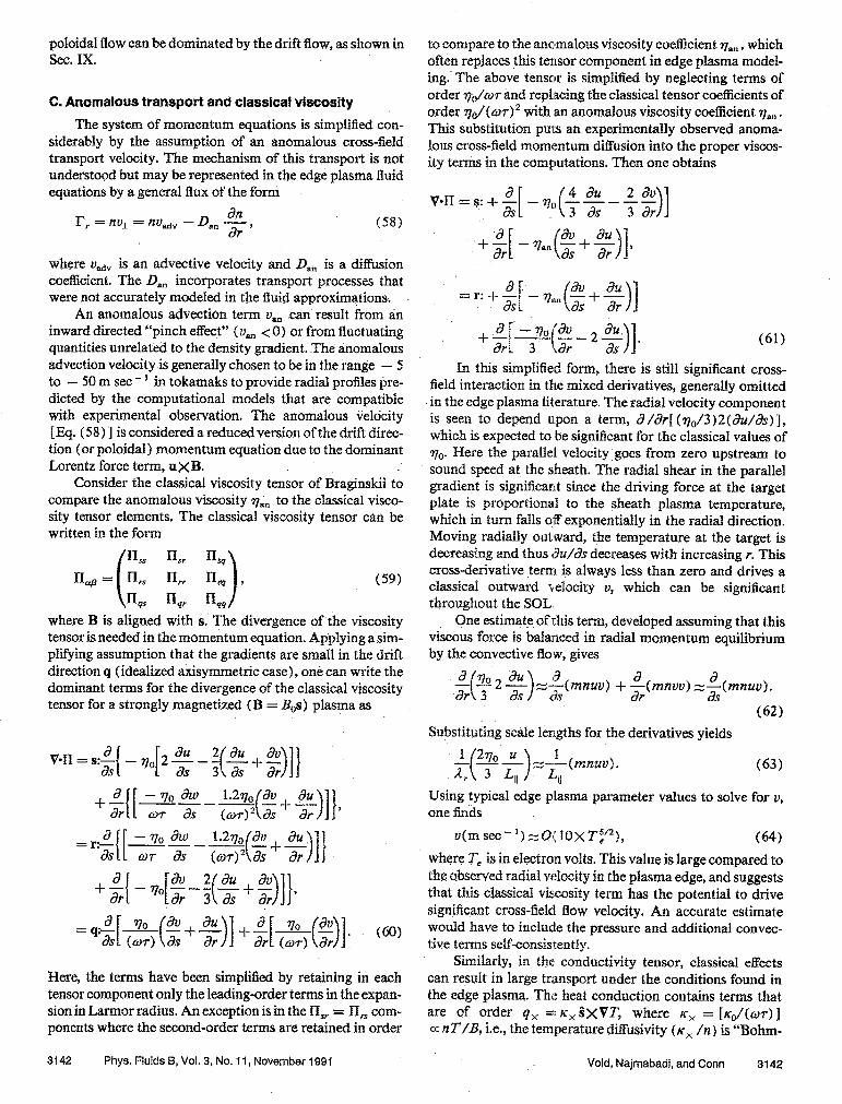
siderably by the assumption of an anomalous cross-field transport velocity. The mechanism of this transport is not understood but may be representedin the edge plasma fluid equations by a general flux of the form

r, = nu, = nu,,, - I&, $,

where v,,, is an advective velocity and Dm is a diffusion coefficient. The D, incorporates transport processes that were not accurately modeled in the fluid approximations.

An anomalous advection term U, can result from an inward directed “pinch effect” (v, < 0) or from fluctuating quantities unrelated to the density gradient. The anomalous advection velocity is generally chosen to be in the range - 5 to - 50 m set - i in tokamaks to provide radial profiles predicted by the computational models that are compatible with experimental observation. The anomalous velocity [IQ. (58) ] is considered a reduced version of the drift direction (or poloidal) momentum equation due to the dominant Lorentz force term, UXB.

Consider the classical viscosity tensor of Braginskii to compare the anomalous viscosity qan to the classical viscosity tensor elements, The classical viscosity tensor can be written in the form

b?=($ g ZJ, (59)

where B is aligned with s. The divergence of the viscosity tensor is needed in the momentum equation. Applying a simplifying assumption that the gradients are small in the drift direction q (idealized axisymmetric case), one can write the dominant terms for the divergence of the classical viscosity tensor for a strongly magnetized (B = B,s) plasma as

v*n=sa 3-I - 7lo[2~-~(-g+$j)

au ‘ar 111

Here, the terms have been simplified by retaining in each tensor component only the leading-order terms in the expansion in Larmor radius. An exception is in the II, = IIrs components where the second-order terms are retained in order

to compare to the anomalous viscosity coefficient ‘)~an, which often replaces this tensor component in edge plasma modeling.~ The above tensor is simplified by neglecting terms of order vo/or and replacing the classical tensor coefficients of order Q/(CCW)~ with an anomalous viscosity coefficient r],, . This substitution purs an experimentally observed anomalous cross-field momentum diffusion into the proper viscosity terms in the computations. Then one obtains

v*n=s:+$ [ ( -‘7” $$-f$ >I ‘+-$[ -Tlan(g+$J],

=r:+$[ -T2,n($+$)] - 7jo /au +g--- -. I 1 2 atf

3 a h r as >i (61)

In this simplified form, there is still significant cross- field interaction in the mixed derivatives, generally omitted in the edge plasma literature. The radial velocity component is seen to depend upon a term, a /&[ ( go/3)2(du/ds) 1, which is expected to be significant for the classical values of qe. Here the parallel velocity goes from zero upstream to sound speed at the sheath. The radial shear in the parallel gradient is significant since the driving force at the target plate is proportional to the sheath plasma temperature, which in turn falls off exponentially in the radial direction, Moving radially outward, the temperature at the target is decreasing and thus trlu/ds decreases with increasing r. This cross-derivative term is always less than zero and drives a classical outward velocity U, which can be significant throughout the SOL.

One estimate of this term, developed assuming that this viscous force is balanced in radial momentum equilibrium by the convective flow, gives

$(?2$-)4 (mnuul + -$(mnuu) ~~(mnuv).

(62) Substituting scale lengths for the derivatives yields

2-l(mnuv). 4

(63)

Using typical edge plasma parameter values to solve for 0, one finds

v(msec-‘)~0ilOXT~‘*), (64) where T, is in electron volts. This value is large compared to the observed radial velocity in the plasma edge, and suggests that this classical viscosity term has the potential to drive significant cross-field flow velocity. An accurate estimate would have to include the pressure and additional convective terms self-consistently.

Similarly, in the conductivity tensor, classical effects can result in large transport under the conditions found in the edge plasma. The heat conduction contains terms that are of order qX =: K, &VT, where K, = [KD/(wT) ]

cc nT/B, i.e., the temperature diffusivity (K, /n) is “Bohm-

3142 Phys. Fluids 8, Vol. 3, No. 11, November 1 BBI Void, Najmabadi, and Conn 3142


like,” a T/B. In ideal MHD core plasmas, temperature gradients are normal to the magnetic flux surfaces, and when crossed with the B-field direction will lead to heat flux along a magnetic flux surface. However, in the edge plasma, where poloidal gradients in temperature can be large, classical heat conduction could lead to “Bohm-1ike”radial heat fluxes.

In Sec. IV the plasma edge equations were derived in toroidal coordinates. In the advective component of flux, evaluating V*( nm (uu) ) is straightforward, but considerable simplifications are needed to define the divergence of the momentum flux tensor. The difficulty arises in evaluating the tensor components of V*(nm(w) > in two different coordinate systems, since (w) is conveniently evaluated in the (s,r,q) coordinates aligned with the magnetic field, but the V*( ) operator is evaluated in the (B,r,$) toroidal or in the flux surface coordinate system.

A classical radial velocity u,, duke to parallel forces can be derived by combining the parallel 6 and the drift 4 components of Ohm’s law. Applying the metrics for the toroidally symmetric case gives

B4 0.71 JT, B, j, ’ ’ v,, = +------- B2he e de

+Jq+!L. BBeh, (T[, Bu, ne

(65) Under ambipolarity, this remains nonzero due to the parallel thermal force component in the poloidal direction, proportional to VII T, .

The toroidal symmetry projects parallel gradient forces (e.g., the thermal force, a V,, T, ) onto poloidal gradients, which can produce a significant radial velocity or flux when crossed into the B field. This classical flux component is included in the edge computational model of Simonini et aI.” and Void,’ and has been proposed as a significant mechanism in the triggering of the H mode.42

The radial velocity is the sum of the classical contribution and the anomalous terms giving a net radial flux

Dan an r, = nv,, + nv,, - -- h, dr

B, 0.71 are B, js v,, +------ B&h, ~11

(66)

The parallel current (j, ) has been proposed as a possible mechanism to control the edge plasma and confinement pro- perties by divertor (or limiter) plate electric biasing.43 How- ever, if the anomalous advection velocity or diffusion coefficient is a function of parallel current, for example, D, = D, (jy) and y is positive, then biasing may have harmful effects on confinement. Biased SOL studies4345 are encouraging and show that under some bias conditions in- creases in confined plasma density are observed.

D. Flux-limited electron conductivity The parallel electron thermal conductivity is evaluated

in the flux-limited form.46*47 A flux-limiting factor fql of 0.1 246 is used to correct the classical conductivity K, _ c, to a flux-limited parallel conductivity, K, _ ,, , in the form”

Ke-” = [ 1 + @e--cl ca~>isj/f,,nC’sTJj ’ (67)

Computational results suggest that this flux-limited factor can be quite significant. Parallel heat flow estimated with classical electron heat conductivity K, _ Cl in the form

may overestimate the parallel heat flow by as much as an order of magnitude. One must be cautious in interpreting results using this estimate in edge plasma analyses.48

The flux-limited parallel heat transport is “anomalously” small compared to the classical value. Simultaneously, the cross-field flux (of heat and momentum) is anomalously large compared to classical or neoclassical predictions. This hints that an appropriate coupling of the parallel and cross- field components, possibly through a “turbulent momentum diffusivity,” could allow self-consistent solutions to match the observed “anomalous” results with the momentum lost from the parallel flux contributing to the increased cross- field momentum flux. Such a coupling can result from classical cross-derivative viscosity and conduction terms, as discussed in the previous section. Solving the complete set of equations with the classical terms included and with no “anomalous” transport assumptions could result in realistic solutions in the plasma edge conditions.

VI. REDUCED 2-D SYSTEM OF PLASMA FLUID EQUATIONS

From the general equations and the simplifying assumptions a set of plasma fluid equations are derived as the basis for a computational model. These equations are incorporat- ed in the EPIC computer code.’ The metric is H = h,h,R and the velocity components are u = us + vr + wq, as shown in Fig. 1. The 2-D equations are continuity:

parallel momentum: amd +L

at H

&(,.R [mnu($&) -$$,‘$I]

mnuv-%!??!- h, Jr )I

+ gp = sp (no)% 6

radial flux: rr = nv,

(70)

4, an = nv,, + nv,, - - - h, dr

B, 0.71 are u,,+--- Da, an B*h, e de

---; h, dr (71)



ion temperature: a($& 1 -+$$(h,R [~~Ti(~*)-(~~~]} +~$[h,R(-$nT,ii-yz)]

a~~{-$[hJt(~~)] +$(h,Ru)]=Q~ +s,(nol~ - USpi( - VS,~(%j), + sn (noI (m/2) (U* + d);

electron temperature: (72)

a(.$nTe> -+$$[h,.R [~~T~(~~)-(~~)~]] at

+tT,v-+ r +)] +$($[h,R(~u)] +j$&d) = -QA f+‘Xee(no). (73)

The ambipolar approximation for the plasma potential Q is evaluated from the poloidal component of the parallel Ohm’s law,

BlJ -C@= BhedB .,iifaa pe + y s Te + @(n,)s,

(74) and the radial component of ion momentum gives an expression for the drift velocity w,

175)

Vll. PLASMA-NEUTRAL MODEL The plasma-neutral source terms required in the fluid

plasma edge model are given. The approach used is the neutral diffusion approximation for neutral transport in a pla$ ma described in detail in a separate paper.’ A brief summary is given here,

The neutral-plasma volumetric source terms are written in a simple manner for the two reactions, electron impact ionization, (a~) ei, an absorption event for neutrals, and charge exchange, ( CW)~~, a scattering event for neutrals. The source term for the continuity equation is

% (noI = nng(Wu),i (76) and the source terms for the ion, electron, and net plasma momentum equations are Sp-e(n~) E - nno(~),i%%.9 (77) Sp- i(nO> ~~~()(~)eirnC&j + nnO(cIu)cx (mOv*cf - mi”f17

(78)

S,(no) ~nno(~)eim&d + nnO(~)cx (mOvOd - mi”i>*

(79) Source terms for the energy or temperature equations are

S,(nO) GZnno(av),i(EO + *) + nnO(m10

x[(Eo+yy+i+Eg], (80) S,(n,)= - nnO(ov)eiEioniz% (81) where E. is the average neutral energy and v,, is the neutral fiuid diffusion velocity given by the diffusion assumption as V od = - (D,/n,)Vn, The neutral diffusion coefficient,

B,, is discussed elsewhere’s9 and defined in the following equation (86) + The value Eionjz = f( &n) is the electron energy loss per ionization due to radiative losses.

The neutral contribution term to Ohm’s law, dP(n,), can be calculated from Eq. ( 17), using (77) and (78). Typi- cal plasma values sh.ow that it can generally be neglected in the edge.

The continuity equation for neutral density no is

~+V-WJ = -S,(n,> = -nno(LTu),,. (82)

The second moment of the neutral transport equation gives an expression for the neutral current flux, I+“, :

r n, == ( -~W3)V*(W,), (83)

yielding a “conservative flux form” of the neutral diffusion equation:

- A*, ~ V( n,u,) >

= 3

- S, (no) = - nno(a-v)ei.

(84) The average speed of the neutrals u. is required to evalu-

ate the neutral density. A simple approximation is that the neutrals are in one energy group and locally at the same energy as the average ion temperature. This one group ion temperature equilibrium (OGITE) approximation leads to the neutral diffusion approximation

an0 at + V*( - D,,Vno) = -S,, (~0) = - na,(m),i

(85) with the neutral diffusion coefficient D, defined as

D& FEE ( - &/3)u,= - #;/3n(cru),,,. (86) At outward directed flux and an inward directed flux

with particle conservation at the boundary can be combined to yield a generalizes Marshak-type boundary condition appropriate for the neutral diffusion approximation:49

[(I -aV(l +a)](n,ud2) +D, Vn,=S,, (87) where the f sign is chosen so that Vn, is outward directed, Q is a neutral reflection coefficient, and So is an inward directed source at the boundary calculated so that total particle conservation is maintained.

Boundaries at the plasma-vacuum duct interface require that the reff e&ion coefficient for neutrals at that

3144 Phys. Fluids 8, Vol, 3, No. 11, November 1991 Void, Najmabadi, and Conn 3144


boundary, a, be evaluated in analytic approximations, taken from empirical data, or determined from Monte Carlo results for complex geometries. At the core-SOL boundary, neutrals are lost from the SOL region by “diffusive” transport into the core edge or “neutral edge” region. The boundary condition at the core-SOL interface must realistically estimate the partitioning between particles reflected as neutrals and those reionized in the core plasma. In time-dependent studies, the response time of these edge-core recycling processes must be accommodated in the mode1.7p9

VIII. PLASMA BOUNDARY CONDITIONS (BC)

The SOL geometry using magnetic flux surface metrics is shown in Fig. 3, with the boundaries labeled for reference. These boundaries include the following.

(a) The core-SOL boundary. This boundary condition is specified along the flux surface tangent to the limiter or the divertor separatrix line, or slightly inward radially from these surfaces toward the plasma core to allow a more self- consistent solution. Plasma particles and heat flowing from the core plasma are sources to the SOL plasma.

Neutrals lost across this boundary into the core are reionized and returned or recycled to the edge as plasma. This boundary condition is set as a specified flux, although fixing the plasma density or temperature at this boundary is common practice when attempting comparisons to experi- ment.

(b) The target plate. In a limiter or divertor configuration, magnetic field lines end at a specially designed target plate, where the plasma sheath forms. The plasma is neutralized upon striking the surface, so the sheath-target boundary is a loss of plasma. Particles are returned as neutrals at the target boundary. The temperature boundary conditions are set in the form of a heat flux loss prescribed by sheath theory, as discussed in this section.

(c) Thefirst wall. The radial flux of plasma to the first wall is generally small compared to the parallel flow loss to the target plates. Gradient scale lengths are given large values to correspond to a small diffusive flux at this boundary. The plasma loss is set equal to the neutral source to account for particle recycling from the first wall. Plasma sheath effects are neglected, since the field lines are assumed parallel to the first wall surface.

A portion of the boundary along the first wall is specified to be a duct for pumping neutrals. This boundary is modeled with a neutral flux reflection coefficient [in Eq. (87) ] of less than unity.

(d) Theflow symmetry lines. In many cases it is convenient to model the SOL from a line halfway along the magnetic field connection length in the edge. Assuming a toroidally symmetric device with one poloidal X point (or limiter), this upstream symmetry line will be halfway around the torus poroidally from the X point. At this flow symmetry line, the net parallel flow is zero, and this location is some- times referred to as the “stagnation line.” Symmetry boundaries are modeled by specifying zero flux and setting the velocities and the gradients in transported quantities to zero.

(e) The private J%X boundary. For the divertor case,

this boundary follows the separatrix line from the X point to the target. An estimate for the diffusive flux across this boundary can be specified in terms of a gradient scale length, derived by relating the cross-field flux to the parallel transport while satisfying a simplified continuity equation. An alternative implementation included in the computational model is to extend the grid beyond the separatrix line to the symmetry line of the device where zero gradient conditions can be specified (if drifts are assumed small).

A. Plasma boundary conditions at the core-SOL interface

The approach is to specify a core efflux based on fueling or pumping exhaust rate requirements and self-consistently evaluate the additional flux across the separatrix due to particle recycling. Details of the self-consistent flux at this boundary have been discussed previously.7,9

The core-SOL boundary conditions for the particle flux Ibc and heat flux Qb, cannot be specified independently. They are related through the global confinement times for particles rp and for energy rE in terms of an average core plasma temperature T, as

3nTc rP -3T,7p. -=--- (88)

The core particle confinement time relates to the core fueling flux and does not include the effects of the core-SOL recycling, calculated self-consistently in the edge plasma computation. A ratio of rp/rE - - 2 is assumed as the default value, but other values can be specified. The flux BC can be a function of time to simulate plasma startup conditions and various time-dependent characteristics of the core such as a reduced flux at the L -. H transition, flux “pulses” observed in the ELM’s, or sawteeth propagation from the core to the edge plasma.

There is controversy regarding the choice of boundary condition at the core-SOL boundary, namely whether to employ fixed values for density and temperature, or to fix the flux of particles and power. The flux boundary conditions more accurately reflect the evolving physical process and allow the values of density and temperature to develop self- consistently at this boundary. Ultimately, a coupled core- edge plasma transport computation would avoid the problems associated with the core-edge interface as a boundary.

B. Sheath boundary conditions A sheath boundary condition applies strictly at the plas-

ma-wall interface regardless of angle of incidence of the magnetic field lines. ” In unmagnetized or magnetic fields with oblique incidence, sheath thicknesses are the order of the Debye length, while the sheath thickness for the exactly parallel (field lines with respect to the tangent to the wall) case becomes the order of the ion gyroradius.” The usual convention in edge plasma modeling is followed here, that the sheath forms only at the surface obliquely intercepting the magnetic field lines, the “target” or “plate” of the limiter or magnetic divertor.



TABLE II. Input parameters for the Alcator C-MOD case.

R, (major radius) 0.67 m SOL thickness 0.03408 mm@)) L, (poloidal length) -0.9 m L,, (X point to target) 0.05-0.1 m U-b/B,, f XW B*(R,) 9T nr (grid cells poloidaliy ) 17 ny (grid cells radially) 9

I?, (equilibrium core-SOL LOX 102°m~z se-c-’ fueling flux)

Qb, (equilibrium core-SOL power flux )

0.2MWm-’

foi (fraction of Qb, to the ions) 0.2 rPp- k (time constant for rbc ) 1o-6 set r,- bc (time constant for Qk ) 6~1O-~sec

ad (neutral reflection 0.95 coefficient at duct)

L, (poloidal width of neutral duct)

~~0.1 m

an 1 m’sec-’ litul 1 m*sec-’ AL-e 2m*se.c-’ X..-, 0.5m2sec-’

Expressions for the sheath potential drop show a range in values depending on the analysis, as summarized for several models recently by Bissell et al.” A sheath potential value, eQ, = 3T, to 3.2T, is common in the literature. Plasma fluid” or kinetic modeb53 are applied to evaluate transmission coefficients S, which relate the plasma density flux, electron energy flux, and ion energy flux through the plasma sheath as a function of the sheath potential drop. Setting general flux quantities equal to sheath transmitted quantities yields rn = (nvhheath = an C,, (89) l?Ti = {[@II: + (M/2)v2]v -~:Vl;.),h~~h =Sin C,q:,,

(90) and

rre = [ (;nT, + eG)v - K:VT,lsheath = S,n C,T,. (91)

The density flux transmission coefficient S is set equal to unity, corresponding to the Bohm sheath criterion, This es- tablishes the boundary condition on parallel velocity li:

Y sheath =U=Csq (92) The boundary conditions on temperature are given by the parallel component of the above energy flux relations, where Si and 6, are specified. There is a range of values for the S’s in the literature, namely ai ~2-3.5 and 8, ~5.5-8. Standard practice has been to fix these transmission coefficients as constants in the computations. Default values are Si = 2.5 and S, = 5.5. We find that the SOL plasma results are not sensitive to the exact values used in the numerical computations. The boundary condition on the parallel component of the energy equation is a flux (mixed-type) BC, which is nonlinear because the classica parallel conductivity varies as K/I - cl a T ‘12, and the value of u = C, a T”2.

3146 Phys. Fluids B, Vol. 3, No. 11, November 1991

a.4

0.2

ZE 0.0 N

-0.2

-0.4

-0.6

B Ratio=Bt~t/BpoP

0.4 C1.6

x 63" 1.0

FIG. 4. C-MOD magnetic flux geometry: The ratio of total B field to poloi- da1 B field is shown to highlight the poloidal field going to zero at each X point and at the core plasma center. The ratio is used to project the parallel flow into the poloidal computational plane in the scrapeoff layer.

IX. COMPUTATIONAL RESULTS Results are given using the reduced plasma equations in

Sec. V to model the Alcator C-MOD tokamak54 divertor plasma. Parameters for the C-MOD edge plasma are given in Table II. The calculations solve the coupled plasma-neutral fluid equations in the magnetic flux surface geometry. The MHD solution is generated by the PESTE code,55 as shown in Fig. 3. The magnetic shear&/B is used to accurately project the parallel flow into the poloidal plane. This shear is eva- Iuated from the MHD equilibrium solution and its inverse is shown in Fig. 4. The computational method has been detailed elsewhere.’ Discussion of the recycling is presented separately, ” Modeling res ults have been compared with data from operating tokamaks such as TEXTOR with rea- sonable results.’

Here we focus on the pofoidal flow, on the resulting ambipolar electric fields in the scrapeoff layer, and their implications for a consistent transport picture. The Alcator C-

Vold, Najmabadi, and Conn 3146


PLASMA DENSITY

'Cl.0 6.1 6.2 a'.3 ' ' d.6 0'.7 d.8 6.9 DISTAk:E A:&G B

NEUTRAL DENSITY 0

d

02

80

#a

FD

$d

E

2:

0 r(

0.0 0.1 0.2 0.3 0.4 0.5 0.6 0.7 0.8 0.9 DISTANCE ALONG B

ELECTRON TEMPERATURE

-. ._____________________________ 1

----------I-I-Ij$i’ a0 HZ0 __-.- /.~;~~~~ ____________-__-- __._____-.--- _____.---- ,.,,.______ - _ /y -*” -- _ -- :

‘0 0 6.1 6.2 0'.3 ( 6.6 DISTAiidE AhiJG B

0'.7 d. 8

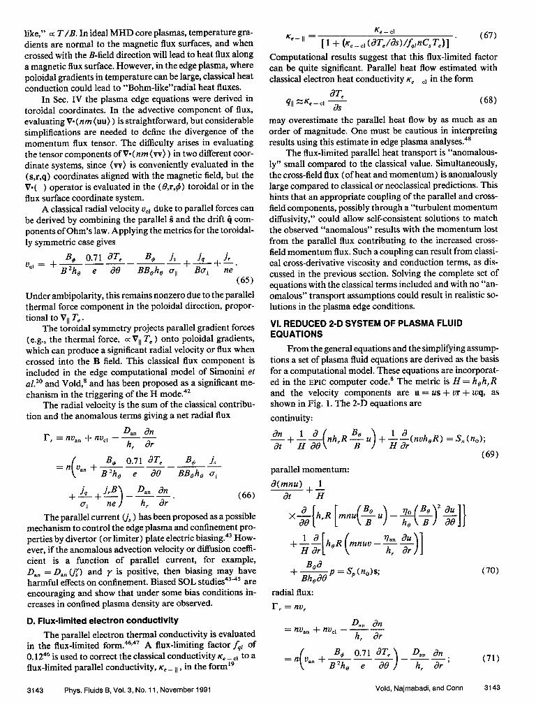
FIG. 5. (a) Plasma density contours (10”’ m-’ ); (b) neutral density contours (10” me3 ); and (c) electron temperature (eV) contours for C-MOD plasma steady state with Pk = 1X10Zom-2sec-‘, and & = 0.2 MW m-‘. The abscissa is distance

along the poloidal B field, the ordinate is a flux surface coordinate. The grid is distorted to emphasize points in the divertor, to the right of x = 0.5. The nonorthogonal target results in the slanted region to the right in the contour plots. The separatrix is at the top, the first wall is at the figures’ bottom.



PARALLEL FLOW VELOCITY 0

0

N

30 2-P E;;- ;’ ii : $- / , I ! / /’ ,,,,,,/ ~~-/,,,;;(,,,,$y I’ ,I’ ,:* -;- 0 ,>>,‘Z : rv‘ :’ ,’ >’ ,r,(re’ ,‘,’ 4, ,’ ! /,c’,:-, EZJ 0 I’ / I , Y’ , (; +;$? / $2 I; ’ : L j’ c ‘I. ‘-.. ;j_l/ .._I : c. I ; 0s f.f

-.__ . ..“. X-i

r( *... *-I -. s-e-:/; I’.:

, I I I I 1 1 / I

0.0 0.1 0.2 0.3 0.4 0.5 0.6 0.7 0.8 4

DISTANCE ALONG B

DRIFT FLQl$- VELOCITY

,, --.*-- _<‘. I, ,I -.-________..- _ ------ -.-*-+-

/ I*

Ku ‘\----.-/A , ’

_,.- ,/’

&- ,_--

~~..--______-________-~---~-------~- *+--

0 e.zt s-l

I 1 1 I I r I t 0.0 0.1 0.2 0.3 0.4 0.5 0.6 0.7 0.8

DISTANCE ALONG B

POLOIDAL FLOW VELOCITY 0

I_--------___ .-____^_---- -,---

__.-c--- __..

‘0.0 d.1 d.2 cl’.3 ’ d.6 DlSTAk:E A&G B

d.7 0‘.8 d

9

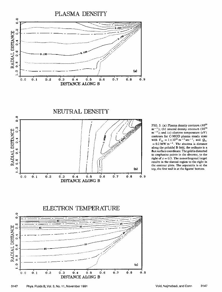
FIG. 6. (a) Parallel velocity contours; (b) drift velocity contours; and (c) poloidal velocity contours ( lo4 m set - ’ ) for the C- MOD plasma steady state with rbc = 1x1020m-2 set’ andQ, =0.2MW

rn-‘.

. 9



PLASMA PoTEmaL (AMBIPOLAR) 0

______c_-------- _----p_p--r-- . . . . . ..______________C_------------------- __________--_----------

“.---.__________----- _______-___--z--p --_--cc-

e-e------- _I’ _____----- _--.._-___________--- ___+___e-so---- (8)

0

d

‘0.0 d.1 d.2 al.3 ’ ’ d-6 d-7 0’.8 6.9 DISTAt& A&G B

POLOIDAL ELECTRIC FIELD

I I I / 0.0 0.1 0.2 0.3 0.4 0.5 0.6 0.7 0.8 0

DISTANCE ALONG B

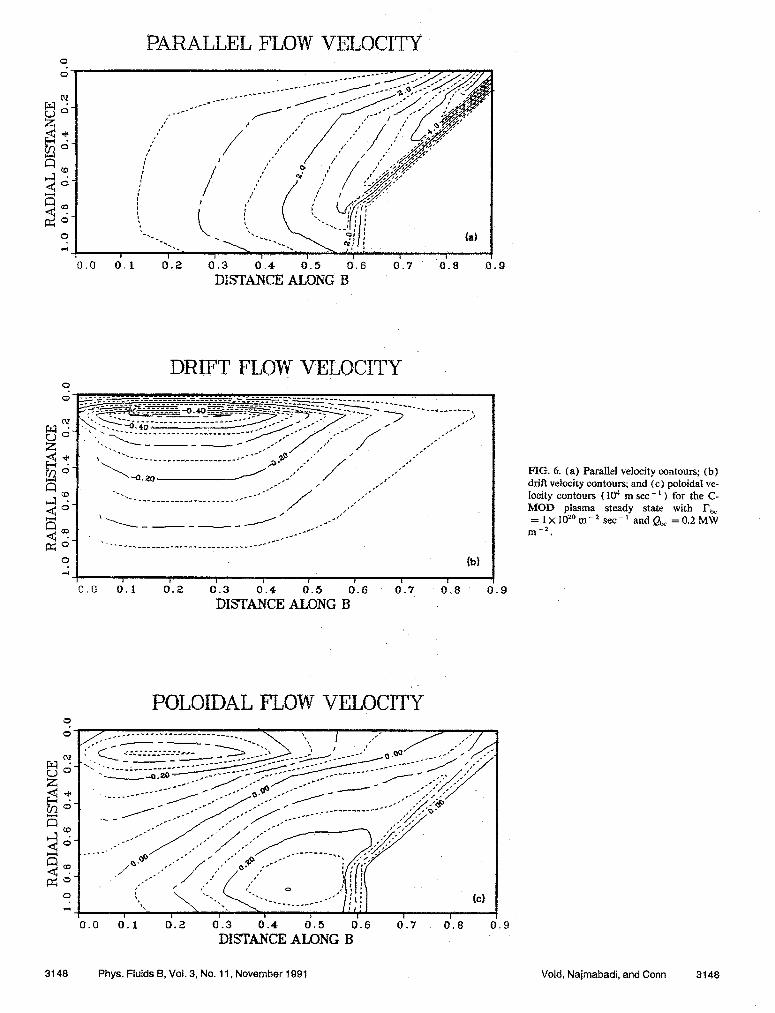
FIG. 7. (a) Ambipolar plasma potential (eV/e); (b) poloidal electric field (V m - ’ ); and (c) radial electric field (V m - ’ ) contours for the C-MOD plasma steady state with I-& = 1 x lozo m-’ set-’ andQ, =0.2MWm-‘.

.9

RADIAL ELECTRIC FIELD

,’ .______--_____-----___ ,’ ,’ ,,’

c 0 (c) d

I I , I I I I I 0.0 0.1 0.2 0.3 0.4 0.5 0.6 0.7 0.8 0.9

DISI’ANCE ALONG B DISI’ANCE ALONG B



MOD results are illustrative of results found for several divertor and limiter tokamak systems. The results provide an opportunity to establish predicted performance prior to experimental operation.

Contour plots of the Alcator C-MOD steady-state results are shown in Figs. 5-7. The results are mapped into a rectangular domain, which emphasizes the divertor region (x > 0.5-0.7 ) , where the computational grid density is grea- test. The abscissa is along the poloidal B field and the ordin- ateis along the magnetic flux surface gradient. Plasma enters from the separatrix along the top of the figures, where the X point is located at about x = 0.7. To the right of the figures, the plasma is neutralized at the nonorthogonal target, leading to the slanted contours seen in the results. The separa- &ix-target intercept is the top right corner of the contour plots.

The coupled quantities, plasma density, neutral density, and electron temperature are shown in Figs. 5 (a)--5 (c). The upstream plasma density radial scrapeoff thickness is about 5 cm for the case of no anomalous advective flux (v,, = 0. f . The plasma density is predicted to peak in the divertor region between the X point and the target. The neutral density peaks at the separatrix-target intercept and falls rapidly across the curved portion of the target plate. The plasma temperature (ion temperature is similar to the electron temperature) is predicted to be 80-100 eV along the core separatrix boundary and to fall to 40-50 eV at the target surface, typical of a “recycling” regime observed in many divertors,57 The extent of the buildup of plasma density and decrease in temperature observed in this divertor is characteristic of a modest recycling regime.

The parallel flow velocity is seen in Fig. 6(a) to be a maximum at the separatrix-target intercept and to fall rapidly away from that point, conforming to the curved target surface. The poloidal drift flux estimated from Pq. (75) is seen in Fig. 6 (b ) to dominate near the core separatrix and is negligible near the target. In this case the toroidal field is directed such that the drift flow is away from the target and opposes the poloidai component of parallel flow. Note that the magnitude of the drift flow is about one-tenth of the parallel flow speed. The combined poloidal flow is shown in Fig, 6(c) and two regions are qualitatively evident. The first is where parallel flow dominates neai the divertor target and the second is where drift flow dominates near the core separatrix, The contour of zero poloidal flow located diagonally across Fig. 6(c), shows where the poloidal components of the oppositely directed drift and parallel flows are of com- parable magnitude. The flow pattern near the other target plate differs considerably where the drift and the parallel flows are in the same direction and thus are additive.

The ambipolar plasma potential [ Pq. (74) ] is shown in Fig. 7 (a). The resulting potential gradient electric fields are shown in Figs. 7(b) and 7(c) for E, and E,, respectiveiy, Poloidal electric fields are negligible in the scrapeoff layer except near the divertor, where the recycling buildup of plasma density leads to EB z 200 V m - ’ , The steep radial gradients upstream lead to radial electric fields of about 16 kVm-‘, with maximum values near the core separatrix. Note that the radial electric field dominates where the poloi-

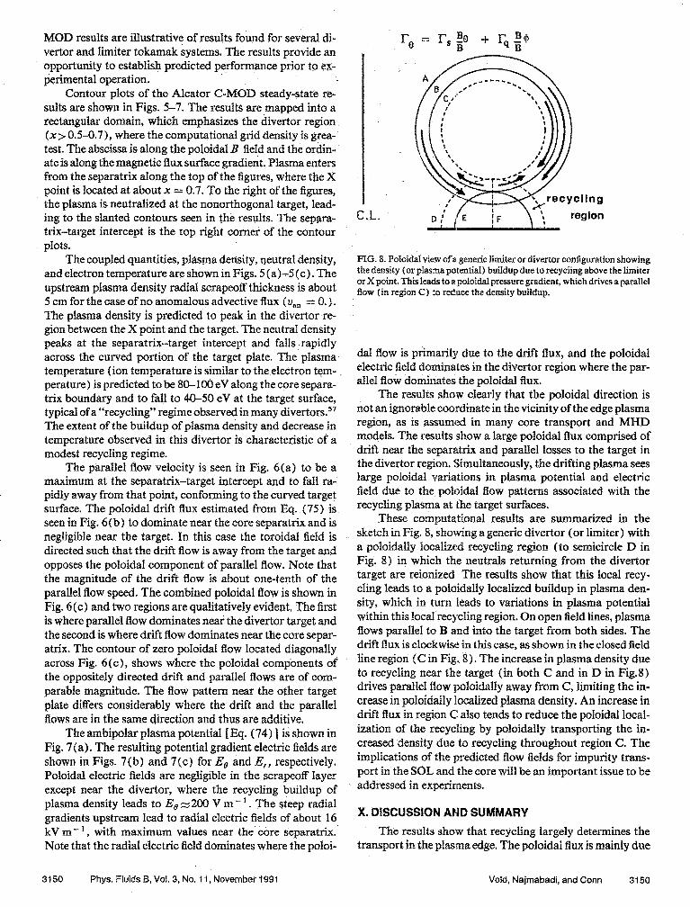
FIG. 8. Poloidal view ofa generic limiter or divertor configuration showing the density (or plasma potential) buildup due to recyciing above the limiter or X point. This leads to a poloidal pressure gradient, which drives a parallel flow (in region C) to reduce the density buildup.

dal flow is primarily due to the drift flux, and the poloidal electric field dominates in the divertor region where the parallel flow dominates the poloidal flux.

The results show clearly that the poloidal direction is not an ignorable coordinate in the vicinity of the edge plasma region, as is assumed in many core transport and MHD models. The results show a large poloidal flux comprised of drift near the separatrix and parallel losses to the target in the divertor region, !$imultaneously, the drifting plasma sees large poloidal variations in plasma potential and electric field due to the poloidal flow patterns associated with the recycling plasma at the target surfaces.

These computational results are summarized in the sketch in Fig. 8, showing a generic divertor (or limiter) with a poloidally localized recycling region (to semicircle D in Fig. 8) in which the neutrals returning from the divertor target are reionized The results show that this local recycling leads to a poloidally localized buildup in plasma density, which in turn leads to variations in plasma potential within this local recycling region. On open field lines, plasma flows parallel to B and into the target from both sides. The drift flux is clockwise: in this case, as shown in the closed field line region ( C in Fig. 8 ) . The increase in plasma density due to recycling near the target (in both C and in D in Fig.8) drives parallel flow poloidally away from C, limiting the increase in poloidally l.ocaIized pIasma density. An increase in drift flux in region C! also tends to reduce the poloidal local- ization of the recycling by poloidally transporting the increased density due to recycling throughout region C. The implications of the predicted flow fields for impurity transport in the SOL and the core will be an important issue to be addressed in experiments.

X. DISCUSSION AND SUMMARY The rest&s show that recycling largely determines the

transport in the plasma edge. The poloidal tlux is mainly due



to drift flow near the separatrix and due to parallel flow near the divertor sheath region. Recycling and transport in the plasma edge region is likely to play a key role in global confinement, since in steady state, the efflux of particles and heat from the core plasma passes through the recycling edge plasma before being pumped or lost to the walls. Recycling involves a coupling of plasma and neutrals that requires a computationally integrated approach. An approach used here incorporates the neutral diffusion model which allows a consistent converged solution to the plasma-neutral problem in a single finite-differenced computational model.

The steady-state radial electric field appears to play a vital role in confinement and is coupled to the edge plasma physics. 38 Consistent models of particle recycling and coupled nonambipolar flows are simultaneously required to fully resolve the edge transport physics. In the toroidally symmetric tokamak, poloidal gradients in the plasma solutions were found in this paper to be imposed on the drift flow, which would result in a poloidal gradient in the drift current for the nonambipolar case. This, in turn, generates radial or parallel currents to maintain a source-free divergence of current, and implies that accurate calculation of the drift flow requires the coupled solution of the three momentum components and the three current (Ohm’s laws) equations. Nonambipolar flow requires an equation for closure, Wj = 0, which can be written explicitly to solve for the steady-state plasma potential [ Eq. (21) ] in the nonambipolar SOL and to extend into the core plasma region.

Poloidal gradients in the edge due to poloidally localized limiters or divertor X points can drive significant, classical radial fluxes of momentum and heat. The large flux of plasma lost to the sheath can drive significant radial transport through the classical viscosity coupling the momentum equations, specifically in the cross-derivative viscosity terms generally neglected in plasma fluid models.

Large poloidal and radial variations in plasma potential are seen in the results. The combination of poloidal gradients and strong poloidal drift flows in the computational results suggests that the mean drifts and fluctuation quantities are coupled in the edge plasma region. We speculate that fluctuations arise because the electric field seen by the plasma changes rapidly as the plasma flows poloidally through the recycling region. Thus there are drift fluctuations proportional to the local recycling and coupled to the poloidal flow. The polarization drift contribution is proportional to U-E. The computed results show that v, -E, and ug * EB are com- parable in magnitude and therefore can be important in coupling fluctuations in the edge. Analytic results supporting this assumption show that a drift wave model with a poloidally periodic forcing function (e.g., poloidal flow through a poloidally localized recycling zone) supports aperiodic or “turbulent-like” solutions. I3

An appropriate computational form to incorporate the “anomalous” transport that results from the coupling of the momentum equations is a modified momentum diffusivity tensor defining the random velocities as a function of the mean velocities to account for the different ion and electron responses driving fluctuation induced transport. There is numerical evidence that modeling the ion (plasma) flux and a

distinct electron (or plasma potential 1 flux yields self-consistent turbulent solutions1*.i3 in 1-D simulations. It remains for a future study to see if that methodology can be implemented self-consistently in a two-dimensional, toroidally symmetric geometry (B,r), and in that case if the “turbulent solution” corresponds to empirically observed “anomalous” levels of cross-field transport.

In evaluating the plasma potential, the nonambipolar flows, and the neutral-plasma coupling, the boundary at the separatrix (or limiter tangency) is found to introduce large uncertainties and reduces the self-consistency of the edge plasma computational calculation. This should be eliminated in future studies by extending the computational grid from the edge plasma into the core center, and by allowing profiles in the closed flux region (the core plasma) to evolve from specified volumetric sources of particles and heat. This would allow one to address issues concerning the effect of the edge plasma on the core plasma transport. A fully coupled edge-core transport calculation would require an integrated MHD calculation based on the full Ohm’s laws discussed in this paper and would require knowledge of the core plasma transport coefficients, a fundamentally difficult problem.

ACKNOWLEDGMENTS This work was performed at the Institute of Plasma and

Fusion Research, University of California at Los Angeles, and supported in part by a grant from the U. S. Department of Energy. The manuscript was completed at the Los Ala- mos National Laboratory, and supported by a Post-Doctor- al Fellowship.

‘P. C. Liewer, Nucl. Fusion 25, 543 ( 1985). *C. M. Surko and R. E. Slusher, Science 221, 817 (1983). %. P. Ritz, D. L. Brower, T. L. Rhodes, and the TEXT team, Nucl. Fusion 27, 1125 ( 1987).

4N. Oyahbu, Nucl. Fusion 9, 149 1 ( 1979). ‘F. Wagner, and the ASDEX team, Phys. Rev. Lett. 49, 1408 ( 1982). 6K. H. Burrel, and the D-III team, in 11th European Conference on Con- trolled Fusion and Plasma Physics, Conference Proceedings at Aachen, 1983 (European Physical Society, Petit-Lancy, Switzerland,l983), Vol. 7D, Part 1, p. 11.

‘E. L. Vold, Ph.D. dissertation, University of California at Los Angeles, 1989.

sE. L. Vold, F.Najmabadi, and R. W. Conn, submitted to J. Comput. Phys. ‘E. L. Vold, A. K. Prinja, F. Najmabadi, and R. W. Conn, J. Nucl. Mater. 176-177,570 ( 1990).

“T Tajima, Computational Plasma Physics: with Applications to Fusion and Astrophysics (Addison-Wesley, New York, 1989).

” K. Theilhaber and C. K. Birdsall, Phys. Fluids B 1,2244,2260 ( 1989). I2 A. Hasegawa and K. Mima, Phys. Fluids 21,87 ( 1978). I3 H. Kaifen and A. Salat, Plasma Phys. Controlled Fusion 31, 123 ( 1989). 14M. Sugihara, S. Saito, S. Hitoki, and N. Fujisawa, J. Nucl. Mater. 128-

129, 114 (1984). “H. Gerhauser and H. A. Claasen, in 12th European Conference on Con-

trolled Fusion and Plasma Physics, Budapest (European Physical Society, Petit-Lancy, Switzerland, 1986), Vol. II, p. 464.

I6 H. Gerhauser and H. A. Claasen (private communication). “B. J. Braams, in IIth European Conference on Controlled Fusion and

Plasma Physics, Aachen (European Physical Society, Petit-Lancy, Swit- zerland, 1983), p. 43 1; also see B. J. Braams, in 12th European Conference on Controlled Fusion and Plasma Physics, Budapest (European Physical Society, Petit-Lancy, Switzerland, 1985), p. 480.



‘*K. Gac and R: Zagonki, to be publishedin J. Nucl.~Mater. I9 B. J, Braams, dissertation, the State University at Utrecht, The Nether-

lands, 1986. “R. Sionini, W. Feneberg, and A, Taroni, in 12th European Canference

OII Cantrailed Fusion and Plasma Physics, Budapest’ (European Physical Society, Petit-Lancy, Switxerhsnd, 1986), p. 484.

“A. Nicolai and P. Biirner, in 12th European Conference an Controlled Fusion and Pkzsma Physics, Budapest (European Physical Society, Petit- Lancy, Switzerland, 1986), p. 519,

*2 Yu. L. Igitkhanov, A. S. Kukushkin, A. Yu. Pigarov, V. I. ‘Pistunovich, in 11th European Conference an ContraNed Fusion and Plasma Physics, Aa- then (European Physical Society, Petit-Lancy, Switzerland, 1983), p. 397.

28 M. Petravic, D. Heifetz, M. Kuo-Petravic, and D. E. Post, J. Nucl. Mater. 12%129,111 (1984).

24S Saito, T. Kobayashi, M. Sugihara, and N. Fujisawa, 3. Nucl. Mater. i&i29,131 (1984).

r5N. Ueda, M, Kasai, M. Tanaka, M. Sugihara, and S. Sengoku, Nucl. Fu- sion28, 1183 (1988).

r6M. Petravic and G. Kuo-Petravic, Nucl. Fusion 30, 1148 ( 1990). *‘N- &da, K. Itoh, and S.-I. Itoh, Nucl. Fusion 29, 173 (1989). “H, Gerhauser and H. A. Claasen, J. Nucl. Mater. 176177,721 (1990). 2q D. Knoll and A. K. Prinja, J. Nucl. Mater. 1X--177,562 ( 1990). 3o S. I. Braginskii, in Reviews of Plasma Physics (Consuhants Bureau, New

York, 1965), VoI. 1. 31 F. L. Hinton and 6. Staebier, in 12th IAEA International Conference an

Plasma Physics and Controlled Fusion Research, Nice, France (IAEA, Vienna, 1988), Vol. II, p. 327; also see F. L. Hinton and G. Staebler, Nucl. Fusion 29,405 (1989).

32B, J. Braams and C. Singer, Fusion Technol. 9,320 ( 1986). a3S. V. Pantankar, Numerical&at TransferandI;iuid57aw (Hemisphere,

New York, 1981). 34R. W. MacConnak, SIAM-AMS Proc. 11, 130 (1978). r5 K. Miyamoto, PZasma Physics far Fusion Engineering (MIT Press, Bos-

ton, MA, 1980). 36P. J. Harbour, I>, D. R. Summers, S. Clement, and the JET team, J. Nucl.

Mater. 162-l&263 (f989).

37B. LaBombard, A. Grossman, and R. W. Corm, J. Nucl. Mater. 176-177. ,548 (1990).

38 K. C. Shaing, Phys. Fluids B 2,764 ( 1990). j9C. E. Sinaer and W. I). Lanaor. Phvs. Rev A 28.994 ( 1983). @R. .I. Tayios M. L. Brown, B. D. Fried, H. Grote, L. R. Liberati, G. J.

Morales, P. Prybal, D. Darrow, and M. Gno, Phys. Rev. Lett. 63,2365 (1989).

“T. Ohkawa and R. L. Miller, Nucl Fusion 30, 1616 ( 1990). 42F. L. Hinton, Nucl. Fusion 25, 1457 (1985). 43R. W. Corm, D. M. Coebel, W. K. Leung, G. A. Campbell, B. LaBom-

bard, A. K. Prinja, W. L. Hsu, and G. J. Thomas, in 11th IAEA Canfer- ence Praceedimgs an Plasma Physics and Controlled Nuclear Fusion Re- sear&. Kyoto (IAEA, Vienna, 1987), Vol. 1, p. 249.

u L. Oren, L. Keller, F. Schwirzke, S. Talmadge, and R. J. Taylor, J. Nucl. Mater. x11-112,34 ( 1982).

“P E. Phillips, A. J. Wooten, W. L. Rowan, and the TEXT team, J. Nucl. Mater. %&S-147,807 1; 1987).

46 J. F. Luciani, P. Mora, and J. Virmont, Phys. Rev. Lett. 51,1664 ( 1983). 47P, Mora and J. F. Luciani, in International Conference an Plasma Physics,

Kiev, USSR (World Scientific, Riveredge, NJ, 1987), Vol. II, p. 755. ‘s P. J. Harbour, Nucl. Fusion 241211 (1984). @M. 2. Hasan and R. W. Corm, J. Comput. Phys. 71,371 ( 1987). SIR. Chodura, in Physic.r ofPlasma- Wall Interactions in Controlled Fusion,

edited by D. E. Post and R. Behrisch (Plenum, New York, 1986), p. 99. ” R C. Bissell, P. C. Johnson, and I? C. Stangeby, Phys. Fluids B 1, 1133

(1989). sP. C. Stangeby, in Physics of Plasma- WallInteractions in Controlled Fu-

sion, edited by D. E. P,)st and R. Behrisch (Plenum, New York, 1986), p. 41.

“G. Emmert, R. Wielald, and A, Mense, Phys. Fluids 23,803 (1980). “1. H. Hutchinson and the Alcator group, in Proceedings of the IEEE 13th

Sympasium on Fusion Engineering, Knoxville, TN, Get 2-6,1989 (IEEE, New York, 1990), p. 13.

“R. C. Grimm, J. M. Greene, J. L. Johnson, Methods Comput. Phys. 16, 253 (1976).

56E L Void, F. Najmabadi, and R. W‘ Corm, submitted to Nucl. Fusion. 57P: C!: Stangeby and G M. McCracken, Nucl. Fusion 30, 1225 ( 1990).

3152 Phys. Fluids 8, Vol. 3, No. 11, November 1991 Void, Najmabadi, and Conn 3152


Documents

Fluid model equations for the tokamak plasma edgearies.ucsd.edu/najmabadi/PAPER/A1-026-91-PF-Vold.pdf · Fluid model equations for the tokamak plasma edge E. L. Void,@ F. Najmabadi,