Fluid Mechanics, River Hydraulics, and Floods

John FentonVienna University of Technology

Outline

• Fluid mechanics• Open channel hydraulics• River engineering• The behaviour of waves in rivers• Flooding in Australia, January 2011

Some guiding principles

• William of Ockham (England, c1288-c1348):"when you have two competing theories that make similar predictions, the simpler one is the

better”.• Karl Popper (A-UK, 1902-1994)

Our preference for simplicity may be justified by his falsifiability criterion: We prefer simpler theories to more complex ones "because their empirical content is greater; and because they are better testable". In other words, a simple theory applies to more cases than a more complex one, and is thus more easily falsifiable.

• Kurt Lewin (D-USA, 1890-1947) "There is nothing so practical as a good theory" – stated in 1951.• R. W. Hamming 1973: “The purpose of computing is insight, not numbers“

In engineering, however, we often need numbers. However, sometimes preoccupation with numbers obscures insight. Often we forget that we are modelling.

• Beauty Is Truth and Truth is BeautyIn 2004, Rolf Reber (University of Bergen), Norbert Schwarz (University of Michigan), and Piotr

Winkielman (University of California at San Diego) suggested that the common experience underlying both perceived beauty and judged truth is processing fluency, which is the experienced ease with which mental content is processed. Indeed, stimuli processed with greater ease elicit more positive affect and statements that participants can read more easily are more likely to be judged as being true. Researchers invoked processing fluency to help explain a wide range of phenomena, including variations in stock prices, brand preferences, or the lack of reception of mathematical theories that are difficult to understand.

Some guiding principles (continued)

• We often lose sight of the fact that we are modelling.• "It is EXACT, Jane" – a story told to the lecturer by a botanist colleague. The most

important river in Australia is the Murray River, 2375 km, maximum recorded flow 3950 cubic metres per second. It has many tributaries, flow measurement in the system is approximate and intermittent, there is huge biological and fluvial diversity and irregularity. My colleague, non-numerical by training, had just seen the demonstration by an hydraulic engineer of a computational model of the river. She asked: "Just how accurate is your model?". The engineer replied intensely: "It is EXACT, Jane".

Fluid Mechanics

• The three-dimensional equations of fluid mechanics govern practically all motion of air and water on the planet.

• The action of viscosity is to act as a momentum diffusion effect – imagine stirring a bucket of water into rotation with a rod if the fluid did not have viscosity

• In civil and mechanical engineering we can usually reduce the problem considerably:• Our flows are usually so large and fast (large Reynolds number) that the flows are

turbulent and the effects of viscosity are relatively small• Our conduits are usually long and thin so that we can integrate across the flow and

consider it to be a one-dimensional problem – consider pipes• We use an empirical law (Darcy-Weisbach) to calculate the resistance to motion (shear

stress on the boundary)• Often the flow changes slowly in time, if at all, and we can consider it to be steady

• Does this apply to rivers?

Top of Control Volume

Water surface

yz

x

q

Q+ΔQQ

Δx

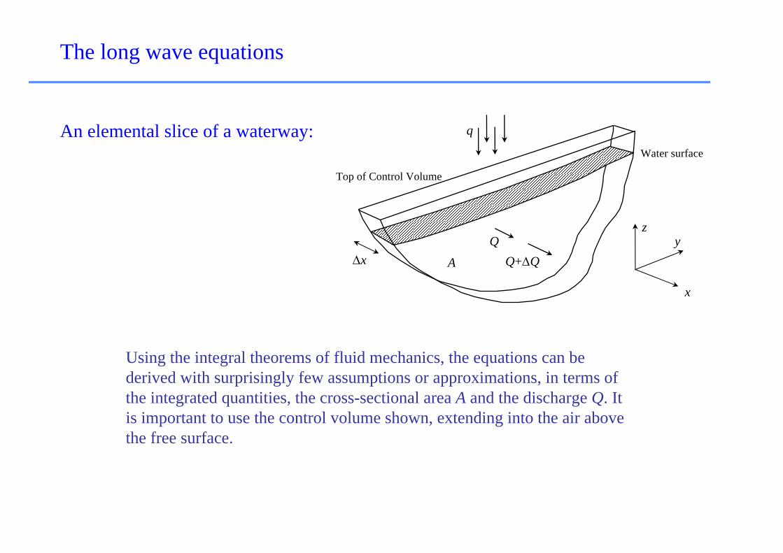
An elemental slice of a waterway:

The long wave equations

Using the integral theorems of fluid mechanics, the equations can be derived with surprisingly few assumptions or approximations, in terms of the integrated quantities, the cross-sectional area A and the discharge Q. It is important to use the control volume shown, extending into the air above the free surface.

A

A Q it x

∂ ∂+ =

∂ ∂

1. Mass conservation equation - in terms of area and discharge

• A is the cross-sectional area, t is time, Q is discharge, x is distance down the channel which is assumed straight for this work, and i is the inflow per unit length.

• Exact (most unusual in fluid mechanics!) for waterways which are not curved in plan.• Linear!

Long wave equations

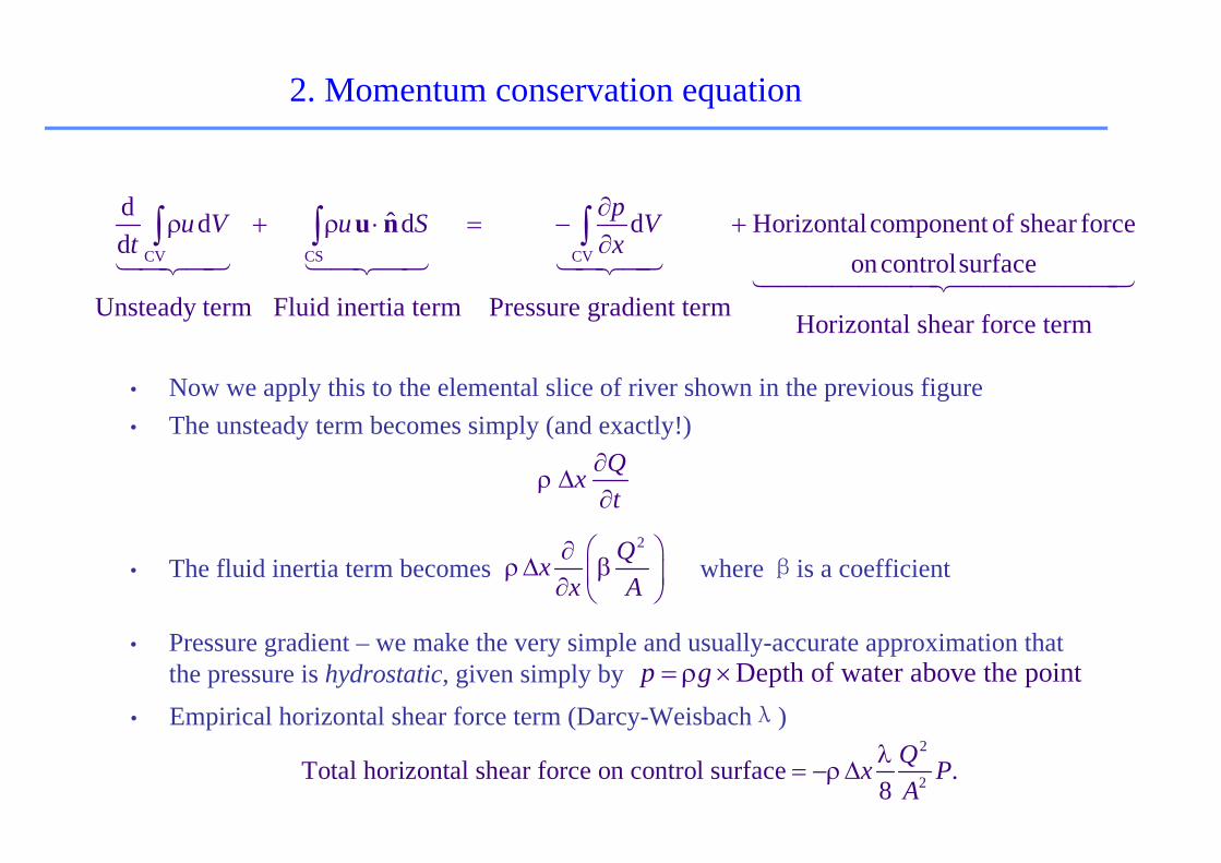
2. Momentum conservation equation

CV CS CV

d ˆd d d Horizontalcomponent of shear forced

oncontrolsurfaceUnsteady term Fluid inertia term Pressure gradient term Horizontal shear force term

pu V u S Vt x

∂ρ + ρ ⋅ = − +

∂∫ ∫ ∫u n

Qxt

∂ρ Δ

∂2Qx

x A⎛ ⎞∂

ρΔ β⎜ ⎟∂ ⎝ ⎠

• Now we apply this to the elemental slice of river shown in the previous figure• The unsteady term becomes simply (and exactly!)

• The fluid inertia term becomes where βis a coefficient

• Pressure gradient – we make the very simple and usually-accurate approximation that the pressure is hydrostatic, given simply by Depth of water above the pointp g= ρ ×

• Empirical horizontal shear force term (Darcy-Weisbachλ)2

2Total horizontal shear force on control surface .8

Qx PA

λ= −ρΔ

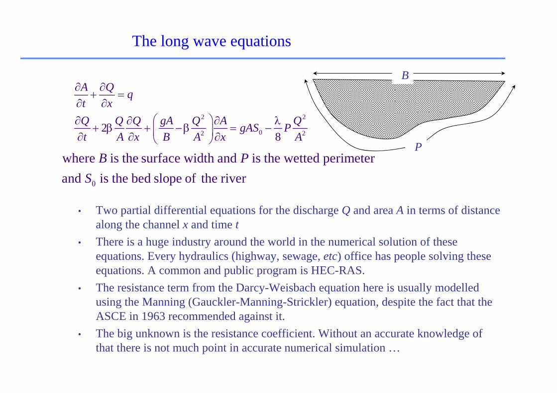
The long wave equations

2 2

02 228

A Q qt xQ Q Q gA Q A QgAS Pt A x B A x A

∂ ∂+ =

∂ ∂⎛ ⎞∂ ∂ ∂ λ

+ β + −β = −⎜ ⎟∂ ∂ ∂⎝ ⎠

0

where is the surface width and is the wetted perimeterand is the bed slope of the river

B PS

B

P

• Two partial differential equations for the discharge Q and area A in terms of distance along the channel x and time t

• There is a huge industry around the world in the numerical solution of these equations. Every hydraulics (highway, sewage, etc) office has people solving these equations. A common and public program is HEC-RAS.

• The resistance term from the Darcy-Weisbach equation here is usually modelled using the Manning (Gauckler-Manning-Strickler) equation, despite the fact that the ASCE in 1963 recommended against it.

• The big unknown is the resistance coefficient. Without an accurate knowledge of that there is not much point in accurate numerical simulation …

Moody diagram

Laminar flow | Transition Zone | Completely turbulent 0.1

0.05

Weisbachfrictionfactor

0.01

103 104 105 106 107 108

Reynolds Number R=UD/

0.07

0.02

0.01

Relativeroughness

0.001

0.0001

0.00001

• At least with this, there are results based on much laboratory evidence.• Manning – there are very few laboratory or field results …

The Gauckler-Manning-Strickler formula for resistance

• The G-M-S formula is widely used – and abused. The resistance coefficient is dimensional, with units of

• It is empirical at best, and has no theoretical justification. The manner in which a value is adopted in practice is most unsatisfactory.

• Typical approaches include:– An Australian approach – using the telephone “You did some work on River X years

ago. What do you think the roughness is on River Y (10km from X) for the reach between A and B?” ).

– Tables of values in books on open channels, given channel conditions, for example books by Barnes for the USA or Hicks and Mason for New Zealand. The photograph is of the Columbia River at Vernita in Washington, taken from Barnes. It has the lowest roughness of all the examples in the book. It is 500m wide and has boulders of diameter … well it doesn't say. Pity, because it is the roughness size to river depth which determines the resistance characteristics. Presenting a picture is not much help – one has little idea of the underwater conditions and how variable they are.

1/3L T−

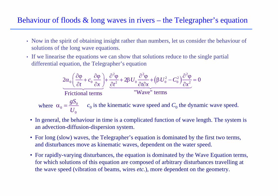
Behaviour of floods & long waves in rivers – the Telegrapher’s equation

( )2 2 2

2 20 0 0 0 02 22 2 0

"Wave" termsFrictional terms

c U U Ct x t t x x

∂ϕ ∂ϕ ∂ ϕ ∂ ϕ ∂ ϕ⎛ ⎞α + + + β + β − =⎜ ⎟∂ ∂ ∂ ∂ ∂ ∂⎝ ⎠

• Now in the spirit of obtaining insight rather than numbers, let us consider the behaviour of solutions of the long wave equations.

• If we linearise the equations we can show that solutions reduce to the single partial differential equation, the Telegrapher’s equation

where 00

0

gSU

α = c0 is the kinematic wave speed and C0 the dynamic wave speed.

• In general, the behaviour in time is a complicated function of wave length. The system is an advection-diffusion-dispersion system.

• For long (slow) waves, the Telegrapher’s equation is dominated by the first two terms, and disturbances move as kinematic waves, dependent on the water speed.

• For rapidly-varying disturbances, the equation is dominated by the Wave Equation terms, for which solutions of this equation are composed of arbitrary disturbances travelling at the wave speed (vibration of beams, wires etc.), more dependent on the geometry.

The first and widely-held view of the nature of wave motion:

• Disturbances propagate at the dynamic wave speed, as most textbooks say.

• This is relatively fast

• It has some important implications: as wave speed increases with depth, higher points on a wave travel faster, and the wave steepens, becomes a flash flood, possibly becoming a bore.

• This is what happened in the recent disastrous events in Queensland in Toowoomba and the Lockyer Valley

View No. 1 of the nature of wave motion

0 DepthC g= ×

Toowoomba (600m)

Escarpment

Lockyer Valley Brisbane

Sudden storm, rapid rise

Steeper (scenes of cars carried at 30 km/h)

Much steeper, very rapid rise Resistance smoothes the front

View No. 2 of the nature of wave motion

• Our second view of the nature of wave motion: In the limit of slow variation, disturbances often behave like slow-moving, diffusing quantities

• They propagate at a kinematic wave speed of roughly 1.5 times the water velocity, not at the dynamic wave speed which most textbooks say.

• In many instances the diffusion is significantly larger than is customary in fluid mechanics, so that the motion appears to be diffusion-dominated and the concept of a wave speed may be relatively unimportant.

• Hence, waves in many rivers do not behave like, well, waves of propagation, but are heavily diffusive.

• This is the behaviour of the large masses of water currently flowing over northern Victoria, where the rain continued for a long time, ground slopes are small, so that there is little opportunity for a bore to develop.

• The vast majority of floods are more of this nature.

To examine better the nature of wave propagation in waterways we used a dynamical program that solved the full long wave equations, forward in time along the channel. With a base flow of 10 m3/s, the inflow was increased smoothly (a Gaussian function of time) by 25% and back down to the base flow over a period of about three hours. The program then simulated conditions in the canal.

10

11

12

0 5 10 15 20

Dis

char

ge (c

u.m

/s)

Time (hours)

InflowOutflow

Example: Canal 2 of Clemmens et al. (1998)

Note heavily-diffusive effects of friction

• The outflow hydrograph is indeed an advected and diffused version of the inflow.

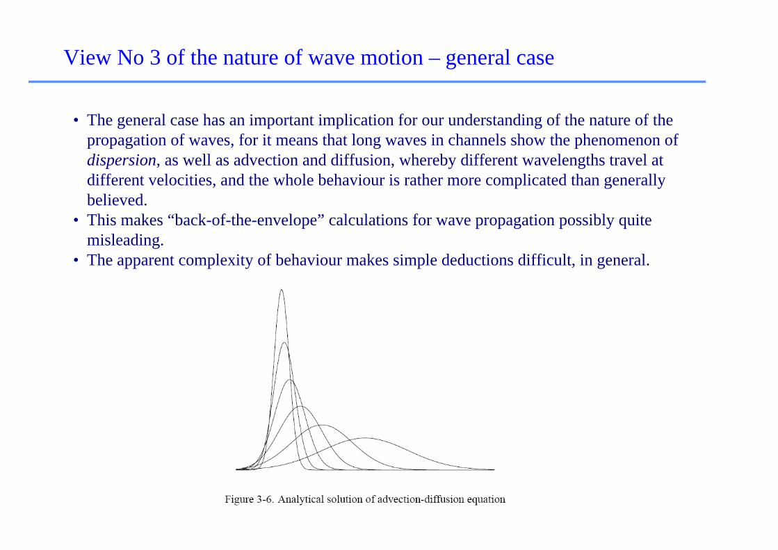
View No 3 of the nature of wave motion – general case

• The general case has an important implication for our understanding of the nature of the propagation of waves, for it means that long waves in channels show the phenomenon of dispersion, as well as advection and diffusion, whereby different wavelengths travel at different velocities, and the whole behaviour is rather more complicated than generally believed.

• This makes “back-of-the-envelope” calculations for wave propagation possibly quite misleading.

• The apparent complexity of behaviour makes simple deductions difficult, in general.

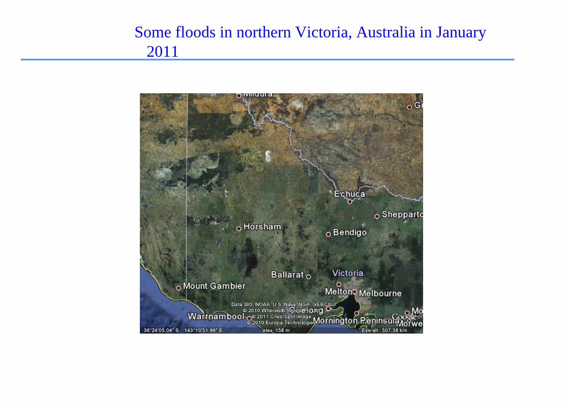
Some floods in northern Victoria, Australia in January 2011

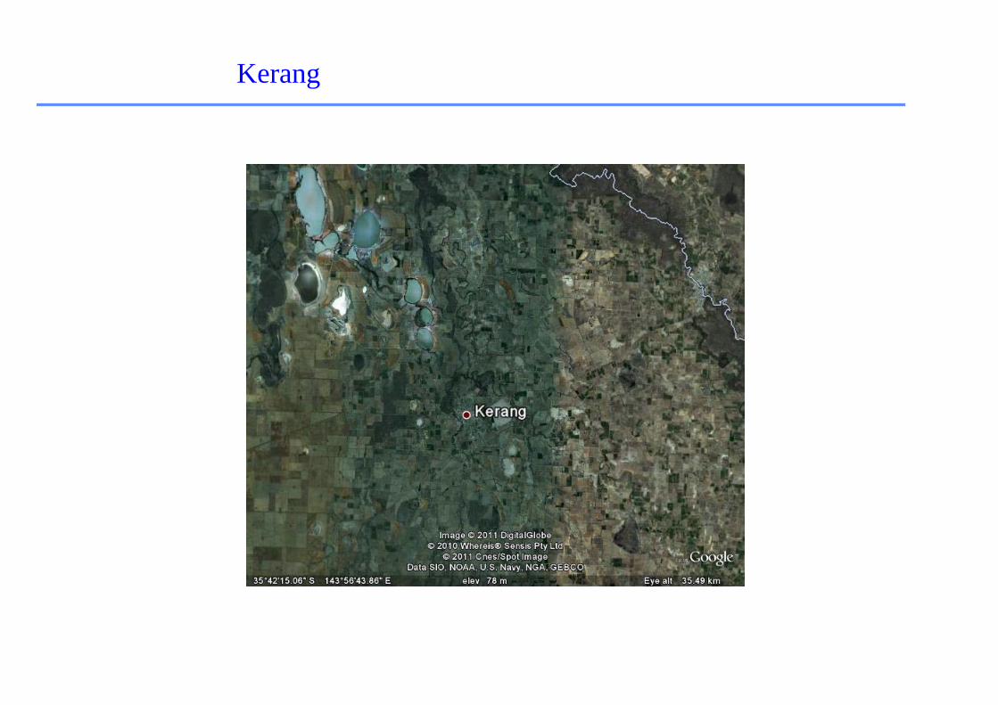
Kerang

Kerang in northern Victoria

• My mother and I had gone from our farm into the town 25km away as she was in a precarious state of health, and we didn´t want to be cut off from the ambulance in case of emergency.

• It was quite a good arrangement, living with three intelligent women with a good wine cellar and where the cook was very good (and me tired of cooking for my mother and me) …

• At 5:30 am two days later the telephone rang, an automatic warning system, and we were advised to leave the town as 150m of levee bank were seeping and in danger of breaking, when the whole town would be flooded.

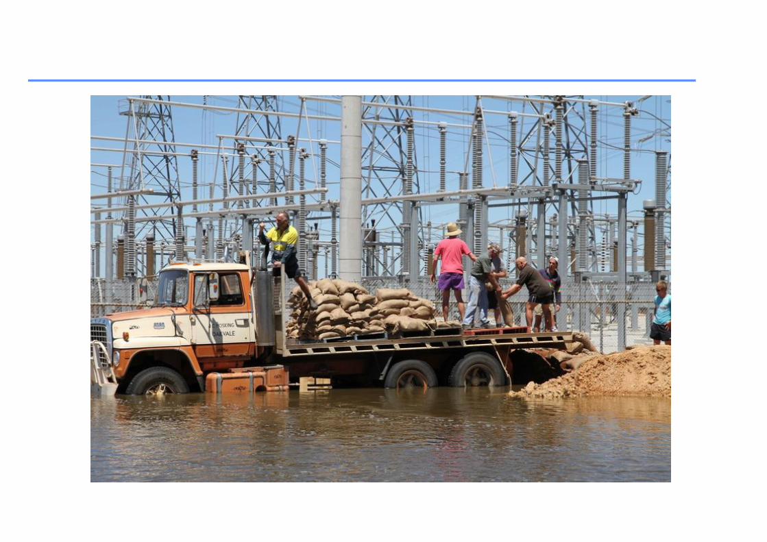
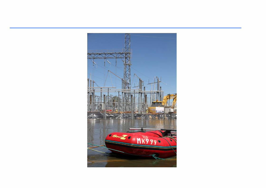
• Worse, some 3km south of the town is a transformer station, which supplies electricity to 20,000 people, and there was greater fear that it would fail, and along with it the water supply and the sewage system, mobile phone chargers, etc etc

• We escaped on the one road possible, into New South Wales, and then slowly south to Melbourne via a rather roundabout route, some 350km.

• The town of Kerang was completely surrounded by floodwater for two weeks, but the town levee bank and the transformer station levee still held.

Meeting of citizens

Monday

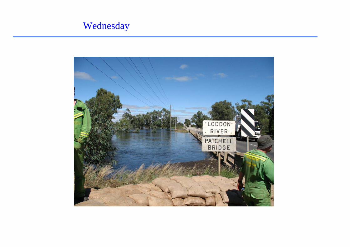
Wednesday

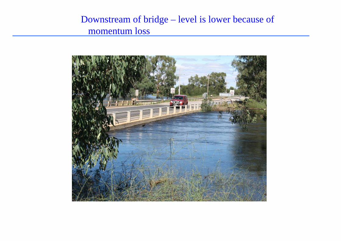
Downstream of bridge – level is lower because of momentum loss

Measuring the water level

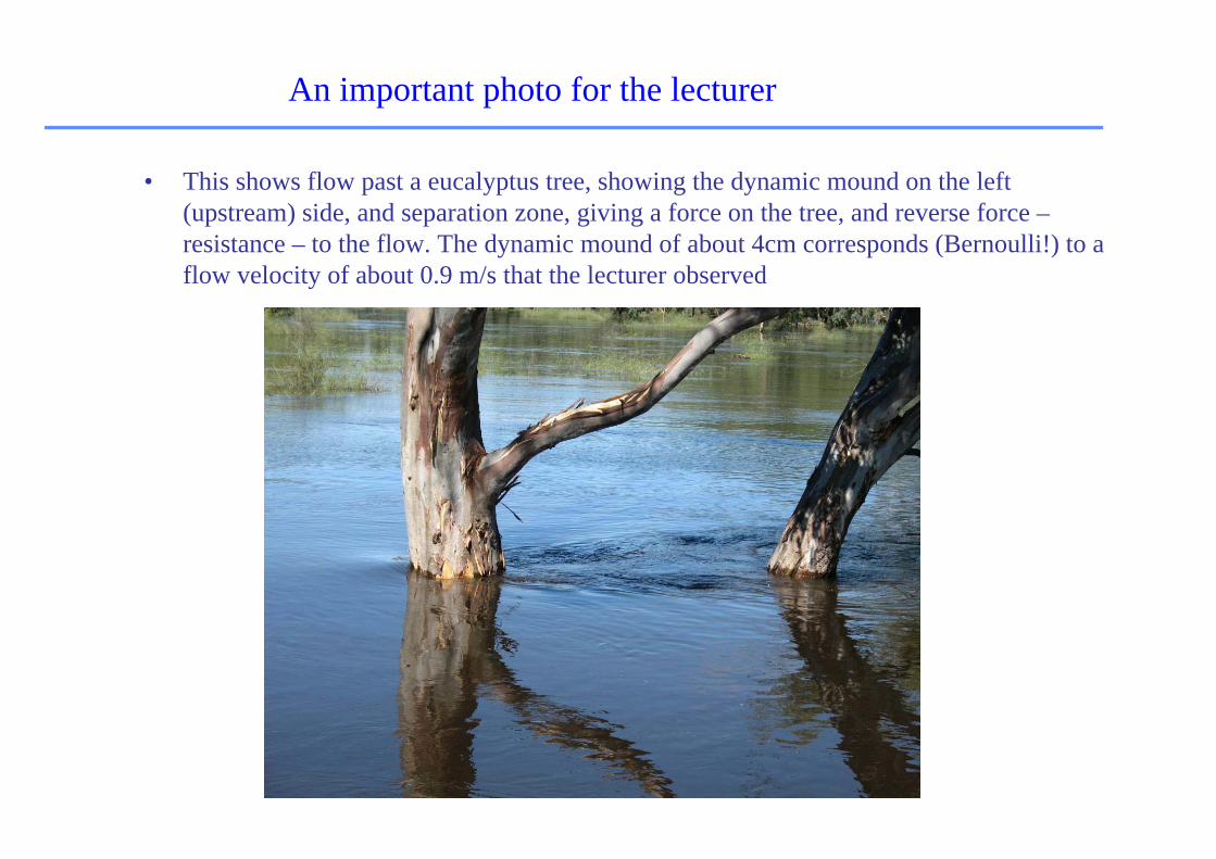
An important photo for the lecturer

• This shows flow past a eucalyptus tree, showing the dynamic mound on the left (upstream) side, and separation zone, giving a force on the tree, and reverse force –resistance – to the flow. The dynamic mound of about 4cm corresponds (Bernoulli!) to a flow velocity of about 0.9 m/s that the lecturer observed

Blocking the highway bridge with sandbags

Later: the most vulnerable point of all – Transformer station

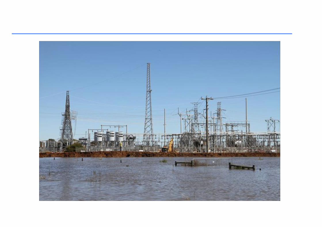
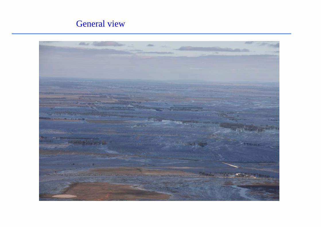
General view

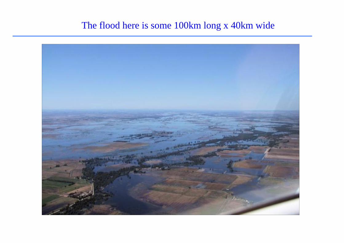
The flood here is some 100km long x 40km wide

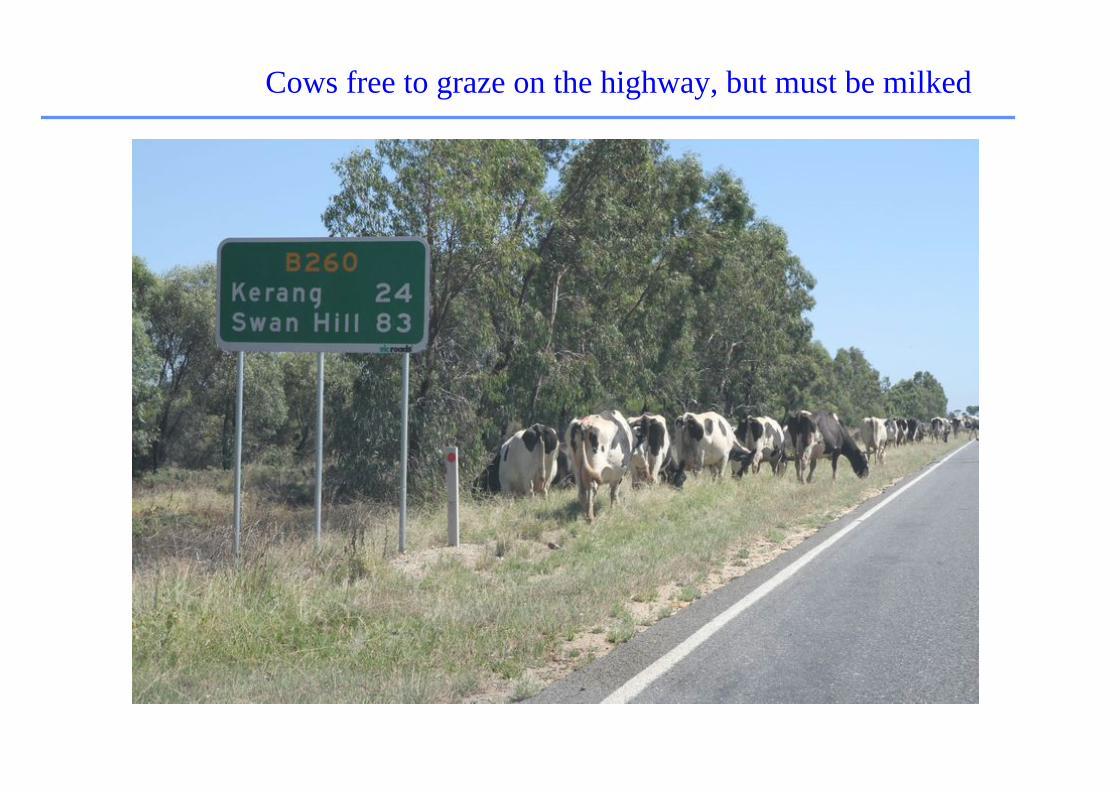
Cows free to graze on the highway, but must be milked

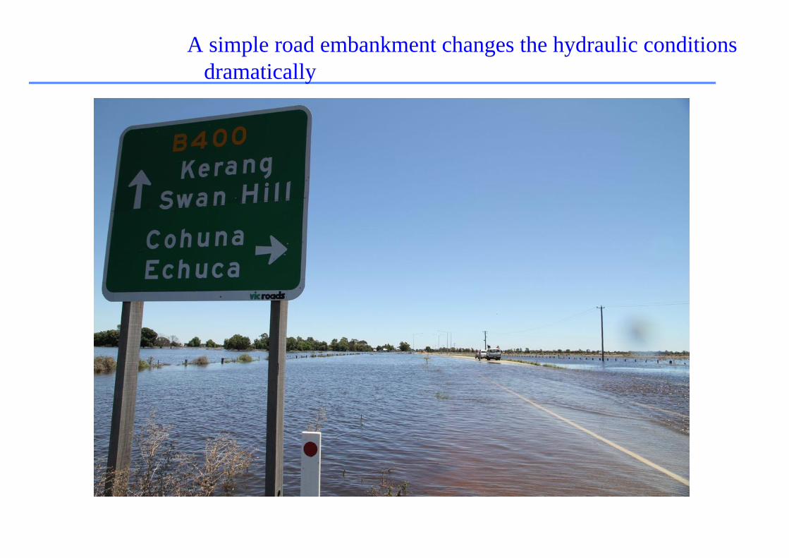
A simple road embankment changes the hydraulic conditions dramatically