Fluid MechanicsChapter 7 – Flow near walls

last edited October 30, 2017

7.1 Motivation 1477.2 Describing the boundary layer 147

7.2.1 Concept 1477.2.2 Why do we study the boundary layer? 1497.2.3 Characterization of the boundary layer 149

7.3 The laminar boundary layer 1517.3.1 Governing equations 1517.3.2 Blasius’ solution 1527.3.3 Pohlhausen’s model 153

7.4 Transition 1557.5 The turbulent boundary layer 1557.6 Separation 157

7.6.1 Principle 1577.6.2 Separation according to Pohlhausen 159

7.7 Exercises 161

These lecture notes are based on textbooks by White [13], Çengel & al.[16], and Munson & al.[18].

7.1 Motivation

Video: pre-lecture brieVng forthis chapter

by o.c. (CC-by)https://youtu.be/kU1m5ojOnUQ

In this chapter, we focus on Wuid Wow close to solid walls. In these regions,viscous eUects dominate the dynamics of Wuids. This study should allow usto answer two questions:

• How can we quantify shear-induced friction on solid walls?

• How can we describe and predict Wow separation?

7.2 Describing the boundary layer

7.2.1 Concept

At the very beginning of the 20th century, Ludwig Prandtl observed that formost ordinary Wuid Wows, viscous eUects played almost no role outside of avery small layer of Wuid along solid surfaces. In this area, shear between thezero-velocity solid wall and the outer Wow dominates the Wow structure. Henamed this zone the boundary layer.

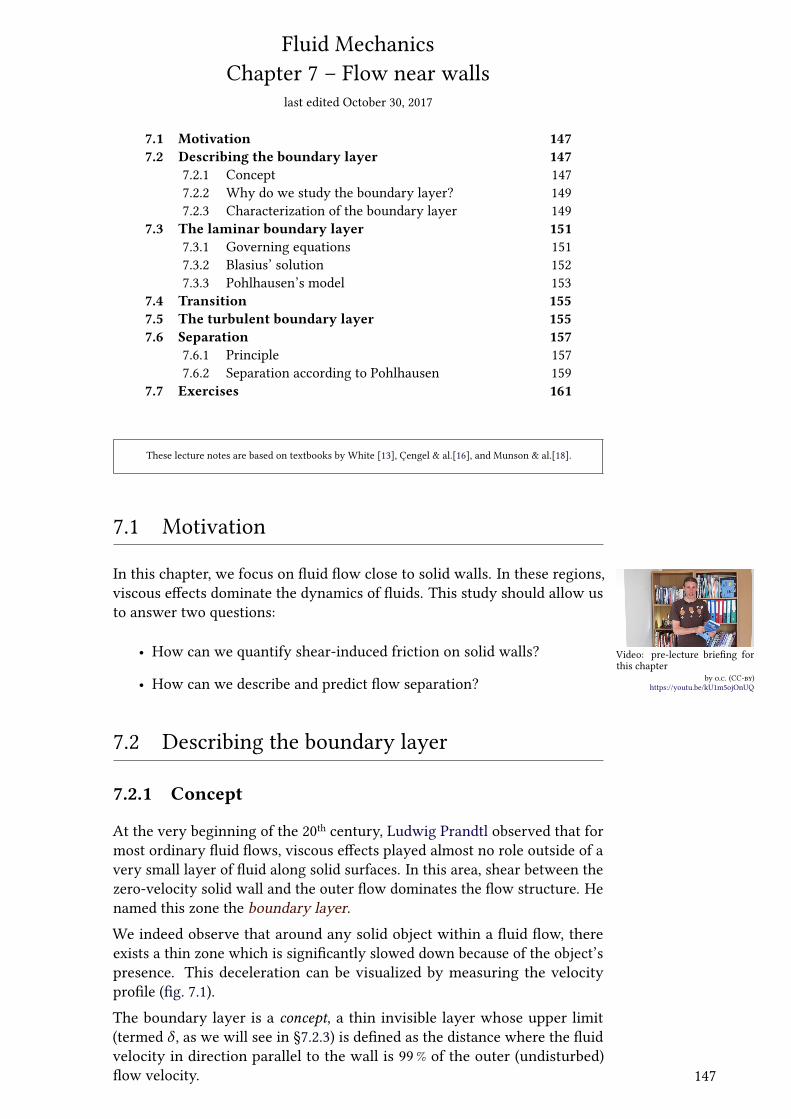
We indeed observe that around any solid object within a Wuid Wow, thereexists a thin zone which is signiVcantly slowed down because of the object’spresence. This deceleration can be visualized by measuring the velocityproVle (Vg. 7.1).

The boundary layer is a concept, a thin invisible layer whose upper limit(termed δ , as we will see in §7.2.3) is deVned as the distance where the Wuidvelocity in direction parallel to the wall is 99 % of the outer (undisturbed)Wow velocity. 147

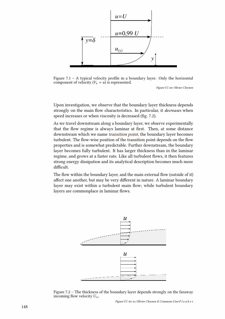
Figure 7.1 – A typical velocity proVle in a boundary layer. Only the horizontalcomponent of velocity (Vx = u) is represented.

Figure CC-by Olivier Cleynen

Upon investigation, we observe that the boundary layer thickness dependsstrongly on the main Wow characteristics. In particular, it decreases whenspeed increases or when viscosity is decreased (Vg. 7.2).

As we travel downstream along a boundary layer, we observe experimentallythat the Wow regime is always laminar at Vrst. Then, at some distancedownstream which we name transition point, the boundary layer becomesturbulent. The Wow-wise position of the transition point depends on the Wowproperties and is somewhat predictable. Further downstream, the boundarylayer becomes fully turbulent. It has larger thickness than in the laminarregime, and grows at a faster rate. Like all turbulent Wows, it then featuresstrong energy dissipation and its analytical description becomes much morediXcult.

The Wow within the boundary layer, and the main external Wow (outside of it)aUect one another, but may be very diUerent in nature. A laminar boundarylayer may exist within a turbulent main Wow; while turbulent boundarylayers are commonplace in laminar Wows.

Figure 7.2 – The thickness of the boundary layer depends strongly on the farawayincoming Wow velocityU∞.

Figure CC-by-sa Olivier Cleynen & Commons User:F l a n k e r

148

7.2.2 Why do we study the boundary layer?

Expending our energy on solving such a minuscule area of the Wow mayseem counter-productive, yet three great stakes are at play here:

• First, a good description allows us to avoid having to solve theNavier-Stokes equations in the whole Wow.Indeed, outside of the boundary layer and of the wake areas, viscouseUects can be safely neglected. Fluid Wow can then be described with

ρ D~VDt = −

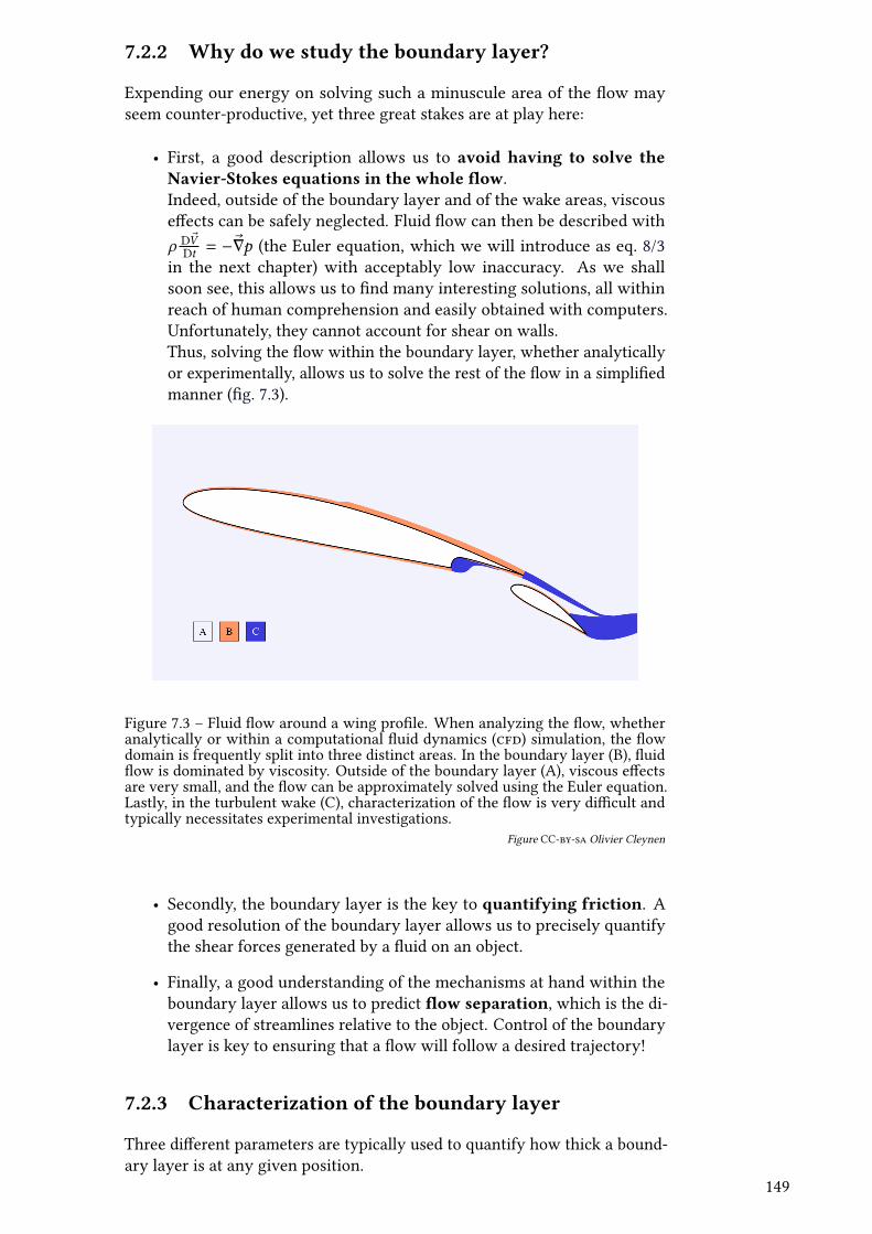
~∇p (the Euler equation, which we will introduce as eq. 8/3in the next chapter) with acceptably low inaccuracy. As we shallsoon see, this allows us to Vnd many interesting solutions, all withinreach of human comprehension and easily obtained with computers.Unfortunately, they cannot account for shear on walls.Thus, solving the Wow within the boundary layer, whether analyticallyor experimentally, allows us to solve the rest of the Wow in a simpliVedmanner (Vg. 7.3).

Figure 7.3 – Fluid Wow around a wing proVle. When analyzing the Wow, whetheranalytically or within a computational Wuid dynamics (cfd) simulation, the Wowdomain is frequently split into three distinct areas. In the boundary layer (B), WuidWow is dominated by viscosity. Outside of the boundary layer (A), viscous eUectsare very small, and the Wow can be approximately solved using the Euler equation.Lastly, in the turbulent wake (C), characterization of the Wow is very diXcult andtypically necessitates experimental investigations.

Figure CC-by-sa Olivier Cleynen

• Secondly, the boundary layer is the key to quantifying friction. Agood resolution of the boundary layer allows us to precisely quantifythe shear forces generated by a Wuid on an object.

• Finally, a good understanding of the mechanisms at hand within theboundary layer allows us to predict Wow separation, which is the di-vergence of streamlines relative to the object. Control of the boundarylayer is key to ensuring that a Wow will follow a desired trajectory!

7.2.3 Characterization of the boundary layer

Three diUerent parameters are typically used to quantify how thick a bound-ary layer is at any given position.

149

The Vrst is the thickness δ ,

δ ≡ y |u=0,99U (7/1)

which is, as we have seen above, equal to the distance away from the wallwhere the speed u is 99 % ofU .

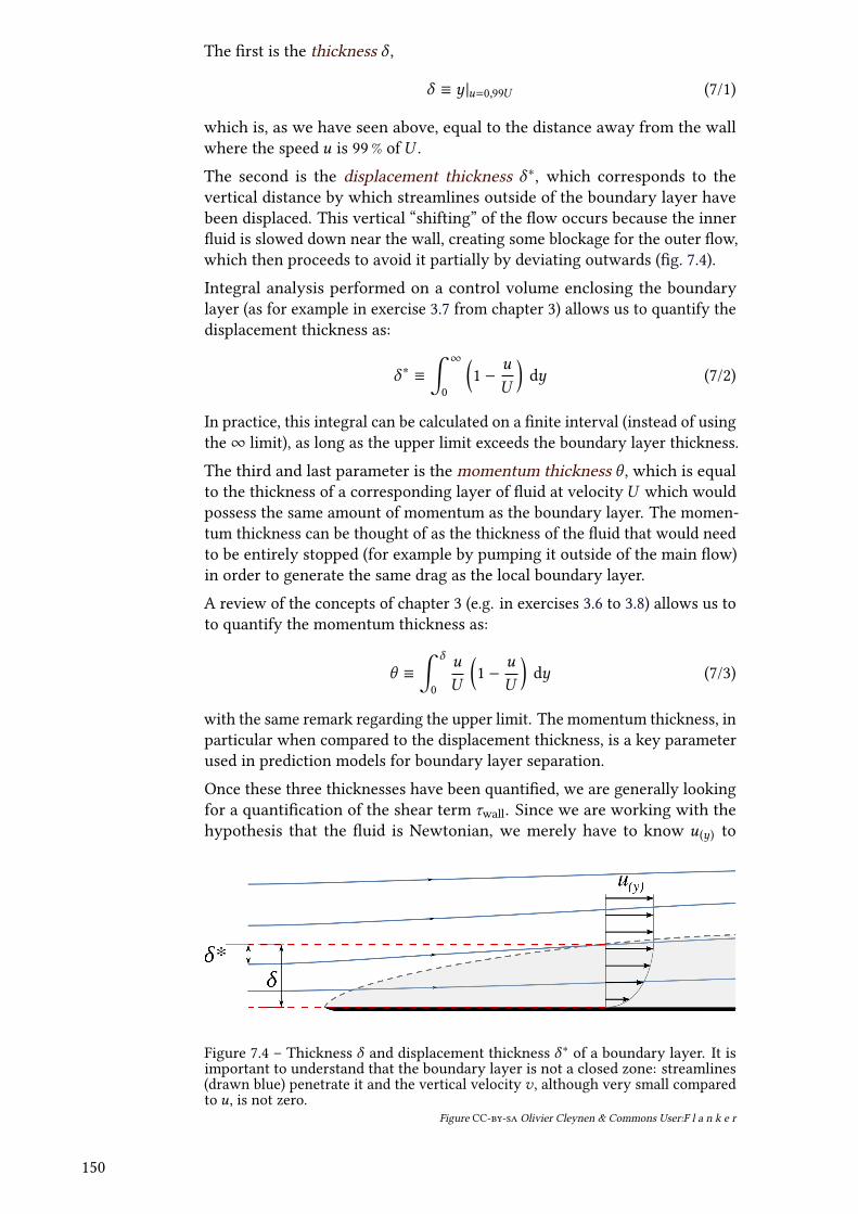
The second is the displacement thickness δ ∗, which corresponds to thevertical distance by which streamlines outside of the boundary layer havebeen displaced. This vertical “shifting” of the Wow occurs because the innerWuid is slowed down near the wall, creating some blockage for the outer Wow,which then proceeds to avoid it partially by deviating outwards (Vg. 7.4).

Integral analysis performed on a control volume enclosing the boundarylayer (as for example in exercise 3.7 from chapter 3) allows us to quantify thedisplacement thickness as:

δ ∗ ≡

∫ ∞

0

(1 −

u

U

)dy (7/2)

In practice, this integral can be calculated on a Vnite interval (instead of usingthe∞ limit), as long as the upper limit exceeds the boundary layer thickness.

The third and last parameter is the momentum thickness θ , which is equalto the thickness of a corresponding layer of Wuid at velocityU which wouldpossess the same amount of momentum as the boundary layer. The momen-tum thickness can be thought of as the thickness of the Wuid that would needto be entirely stopped (for example by pumping it outside of the main Wow)in order to generate the same drag as the local boundary layer.

A review of the concepts of chapter 3 (e.g. in exercises 3.6 to 3.8) allows us toto quantify the momentum thickness as:

θ ≡

∫ δ

0

u

U

(1 −

u

U

)dy (7/3)

with the same remark regarding the upper limit. The momentum thickness, inparticular when compared to the displacement thickness, is a key parameterused in prediction models for boundary layer separation.

Once these three thicknesses have been quantiVed, we are generally lookingfor a quantiVcation of the shear term τwall. Since we are working with thehypothesis that the Wuid is Newtonian, we merely have to know u (y) to

Figure 7.4 – Thickness δ and displacement thickness δ ∗ of a boundary layer. It isimportant to understand that the boundary layer is not a closed zone: streamlines(drawn blue) penetrate it and the vertical velocity v , although very small comparedto u, is not zero.

Figure CC-by-sa Olivier Cleynen & Commons User:F l a n k e r

150

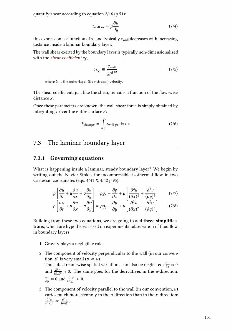
quantify shear according to equation 2/16 (p.51):

τwall yx = µ∂u

∂y(7/4)

this expression is a function of x , and typically τwall decreases with increasingdistance inside a laminar boundary layer.

The wall shear exerted by the boundary layer is typically non-dimensionalizedwith the shear coeXcient c f ,

c f (x ) ≡τwall12ρU

2(7/5)

whereU is the outer-layer (free-stream) velocity.

The shear coeXcient, just like the shear, remains a function of the Wow-wisedistance x .

Once these parameters are known, the wall shear force is simply obtained byintegrating τ over the entire surface S :

Fshearyx =

∫Sτwall yx dx dz (7/6)

7.3 The laminar boundary layer

7.3.1 Governing equations

What is happening inside a laminar, steady boundary layer? We begin bywriting out the Navier-Stokes for incompressible isothermal Wow in twoCartesian coordinates (eqs. 4/41 & 4/42 p.95):

ρ

[∂u

∂t+ u∂u

∂x+v∂u

∂y

]= ρдx −

∂p

∂x+ µ

[∂2u

(∂x )2+∂2u

(∂y)2

](7/7)

ρ

[∂v

∂t+ u∂v

∂x+v∂v

∂y

]= ρдy −

∂p

∂y+ µ

[∂2v

(∂x )2+∂2v

(∂y)2

](7/8)

Building from these two equations, we are going to add three simpliVca-tions, which are hypotheses based on experimental observation of Wuid Wowin boundary layers:

1. Gravity plays a negligible role;

2. The component of velocity perpendicular to the wall (in our conven-tion, v) is very small (v � u).Thus, its stream-wise spatial variations can also be neglected: ∂v∂x ≈ 0

and ∂2v(∂x )2

≈ 0. The same goes for the derivatives in the y-direction:∂v∂y ≈ 0 and ∂2v

(∂y)2≈ 0.

3. The component of velocity parallel to the wall (in our convention, u)varies much more strongly in the y-direction than in the x-direction:∂2u(∂x )2

� ∂2u(∂y)2

.

151

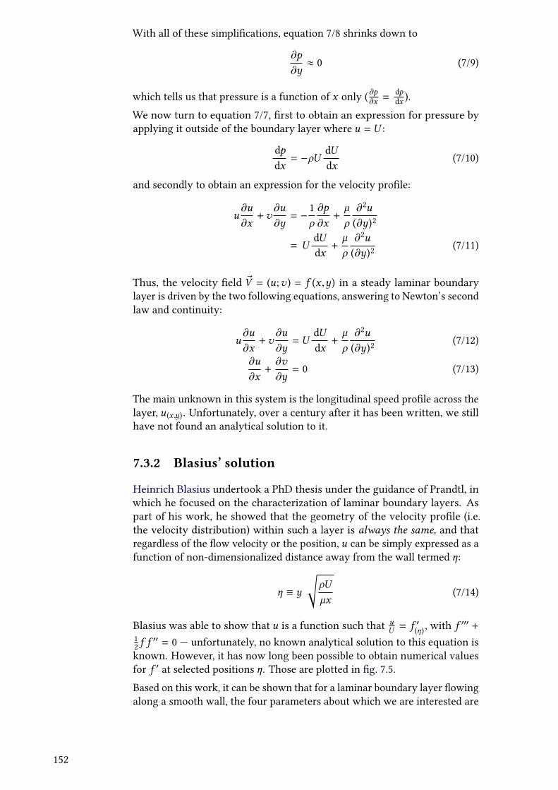
With all of these simpliVcations, equation 7/8 shrinks down to

∂p

∂y≈ 0 (7/9)

which tells us that pressure is a function of x only ( ∂p∂x =dpdx ).

We now turn to equation 7/7, Vrst to obtain an expression for pressure byapplying it outside of the boundary layer where u = U :

dpdx= −ρU

dUdx

(7/10)

and secondly to obtain an expression for the velocity proVle:

u∂u

∂x+v∂u

∂y= −

1ρ

∂p

∂x+µ

ρ

∂2u

(∂y)2

= UdUdx+µ

ρ

∂2u

(∂y)2(7/11)

Thus, the velocity Veld ~V = (u;v ) = f (x ,y) in a steady laminar boundarylayer is driven by the two following equations, answering to Newton’s secondlaw and continuity:

u∂u

∂x+v∂u

∂y= U

dUdx+µ

ρ

∂2u

(∂y)2(7/12)

∂u

∂x+∂v

∂y= 0 (7/13)

The main unknown in this system is the longitudinal speed proVle across thelayer, u (x ,y) . Unfortunately, over a century after it has been written, we stillhave not found an analytical solution to it.

7.3.2 Blasius’ solution

Heinrich Blasius undertook a PhD thesis under the guidance of Prandtl, inwhich he focused on the characterization of laminar boundary layers. Aspart of his work, he showed that the geometry of the velocity proVle (i.e.the velocity distribution) within such a layer is always the same, and thatregardless of the Wow velocity or the position, u can be simply expressed as afunction of non-dimensionalized distance away from the wall termed η:

η ≡ y

√ρU

µx(7/14)

Blasius was able to show that u is a function such that uU = f ′

(η), with f ′′′ +

12 f f

′′ = 0 — unfortunately, no known analytical solution to this equation isknown. However, it has now long been possible to obtain numerical valuesfor f ′ at selected positions η. Those are plotted in Vg. 7.5.

Based on this work, it can be shown that for a laminar boundary layer Wowingalong a smooth wall, the four parameters about which we are interested are

152

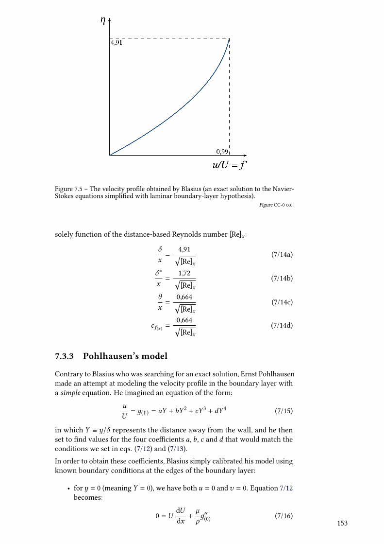
Figure 7.5 – The velocity proVle obtained by Blasius (an exact solution to the Navier-Stokes equations simpliVed with laminar boundary-layer hypothesis).

Figure CC-0 o.c.

solely function of the distance-based Reynolds number [Re]x :

δ

x=

4,91√[Re]x

(7/14a)

δ ∗

x=

1,72√[Re]x

(7/14b)

θ

x=

0,664√[Re]x

(7/14c)

c f (x ) =0,664√[Re]x

(7/14d)

7.3.3 Pohlhausen’s model

Contrary to Blasius who was searching for an exact solution, Ernst Pohlhausenmade an attempt at modeling the velocity proVle in the boundary layer witha simple equation. He imagined an equation of the form:

u

U= д(Y ) = aY + bY 2 + cY 3 + dY 4 (7/15)

in which Y ≡ y/δ represents the distance away from the wall, and he thenset to Vnd values for the four coeXcients a, b, c and d that would match theconditions we set in eqs. (7/12) and (7/13).

In order to obtain these coeXcients, Blasius simply calibrated his model usingknown boundary conditions at the edges of the boundary layer:

• for y = 0 (meaning Y = 0), we have both u = 0 andv = 0. Equation 7/12becomes:

0 = UdUdx+µ

ρд′′(0) (7/16)

153

• fory = δ (meaningY = 1) we haveu =U , ∂u/∂y = 0 and ∂2u/(∂y)2 = 0.These values allow us to evaluate three properties of function д :

u = U = Uд(1) (7/17)∂u

∂y= 0 =

U

δд′(1) (7/18)

∂2u

(∂y)2= 0 =

U

δ 2д′′(1) (7/19)

This system of four equations allowed Pohlhausen to evaluate the four termsa, b, c and d . He introduced the variable Λ, a non-dimensional measure ofthe outer velocity Wow-wise gradient:

Λ ≡ δ 2ρ

µ

dUdx

(7/20)

and he then showed that his velocity model in the smooth-surface laminarboundary layer, equation 7/15, had Vnally become:

u

U= 1 − (1 + Y ) (1 − Y )3 + Λ

Y

6(1 − Y 3) (7/21)

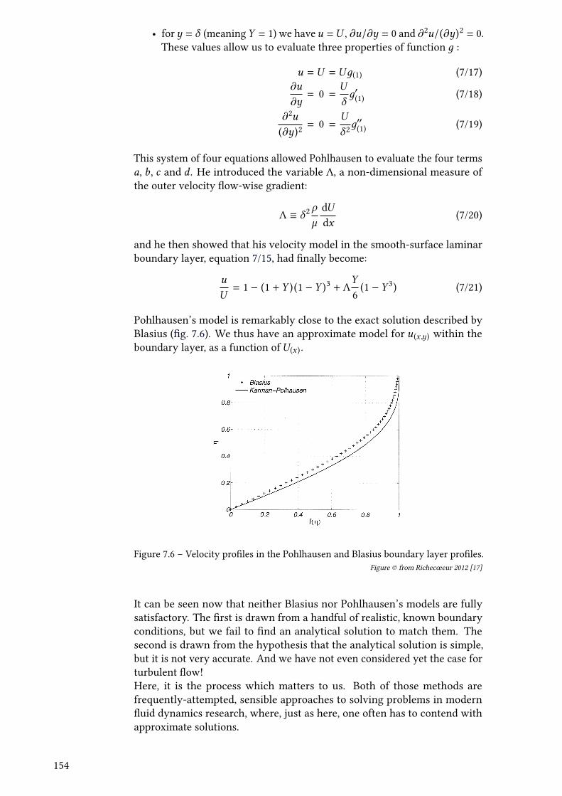
Pohlhausen’s model is remarkably close to the exact solution described byBlasius (Vg. 7.6). We thus have an approximate model for u (x ,y) within theboundary layer, as a function ofU(x ) .

Figure 7.6 – Velocity proVles in the Pohlhausen and Blasius boundary layer proVles.Figure © from Richecœeur 2012 [17]

It can be seen now that neither Blasius nor Pohlhausen’s models are fullysatisfactory. The Vrst is drawn from a handful of realistic, known boundaryconditions, but we fail to Vnd an analytical solution to match them. Thesecond is drawn from the hypothesis that the analytical solution is simple,but it is not very accurate. And we have not even considered yet the case forturbulent Wow!Here, it is the process which matters to us. Both of those methods arefrequently-attempted, sensible approaches to solving problems in modernWuid dynamics research, where, just as here, one often has to contend withapproximate solutions.

154

7.4 Transition

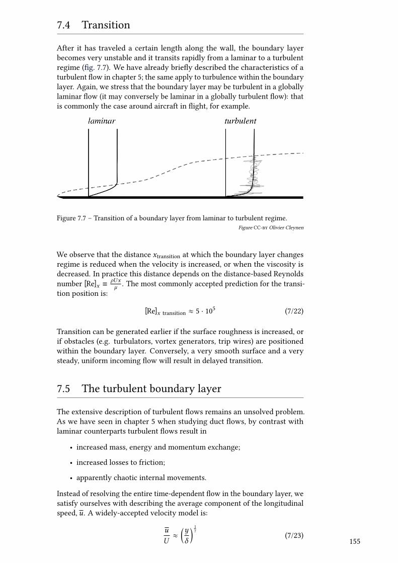
After it has traveled a certain length along the wall, the boundary layerbecomes very unstable and it transits rapidly from a laminar to a turbulentregime (Vg. 7.7). We have already brieWy described the characteristics of aturbulent Wow in chapter 5; the same apply to turbulence within the boundarylayer. Again, we stress that the boundary layer may be turbulent in a globallylaminar Wow (it may conversely be laminar in a globally turbulent Wow): thatis commonly the case around aircraft in Wight, for example.

Figure 7.7 – Transition of a boundary layer from laminar to turbulent regime.Figure CC-by Olivier Cleynen

We observe that the distance xtransition at which the boundary layer changesregime is reduced when the velocity is increased, or when the viscosity isdecreased. In practice this distance depends on the distance-based Reynoldsnumber [Re]x ≡

ρUxµ . The most commonly accepted prediction for the transi-

tion position is:

[Re]x transition ≈ 5 · 105 (7/22)

Transition can be generated earlier if the surface roughness is increased, orif obstacles (e.g. turbulators, vortex generators, trip wires) are positionedwithin the boundary layer. Conversely, a very smooth surface and a verysteady, uniform incoming Wow will result in delayed transition.

7.5 The turbulent boundary layer

The extensive description of turbulent Wows remains an unsolved problem.As we have seen in chapter 5 when studying duct Wows, by contrast withlaminar counterparts turbulent Wows result in

• increased mass, energy and momentum exchange;

• increased losses to friction;

• apparently chaotic internal movements.

Instead of resolving the entire time-dependent Wow in the boundary layer, wesatisfy ourselves with describing the average component of the longitudinalspeed, u. A widely-accepted velocity model is:

u

U≈

(yδ

) 17

(7/23)155

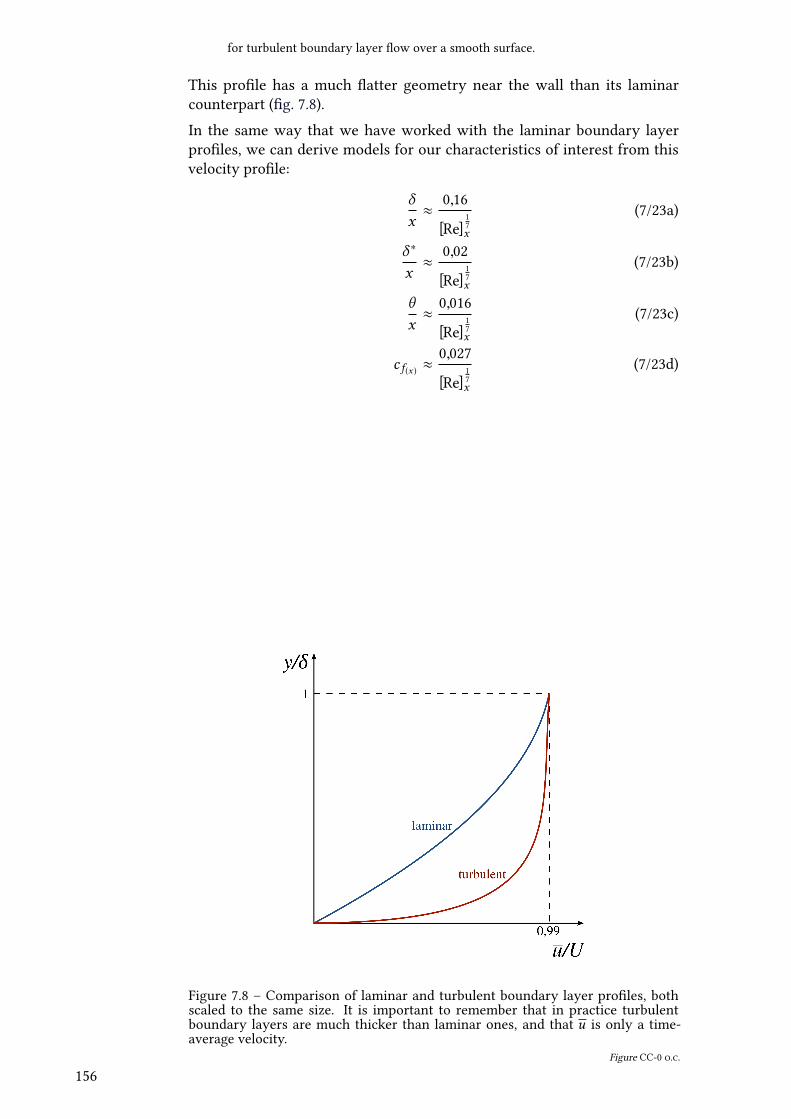
for turbulent boundary layer Wow over a smooth surface.

This proVle has a much Watter geometry near the wall than its laminarcounterpart (Vg. 7.8).

In the same way that we have worked with the laminar boundary layerproVles, we can derive models for our characteristics of interest from thisvelocity proVle:

δ

x≈

0,16

[Re]17x

(7/23a)

δ ∗

x≈

0,02

[Re]17x

(7/23b)

θ

x≈

0,016

[Re]17x

(7/23c)

c f (x ) ≈0,027

[Re]17x

(7/23d)

Figure 7.8 – Comparison of laminar and turbulent boundary layer proVles, bothscaled to the same size. It is important to remember that in practice turbulentboundary layers are much thicker than laminar ones, and that u is only a time-average velocity.

Figure CC-0 o.c.

156

7.6 Separation

7.6.1 Principle

Under certain conditions, Wuid Wow separates from the wall. The boundarylayer then disintegrates and we observe the appearance of a turbulent wakenear the wall. Separation is often an undesirable phenomenon in Wuidmechanics: it may be thought of as the point where we fail to impart adesired trajectory to the Wuid.

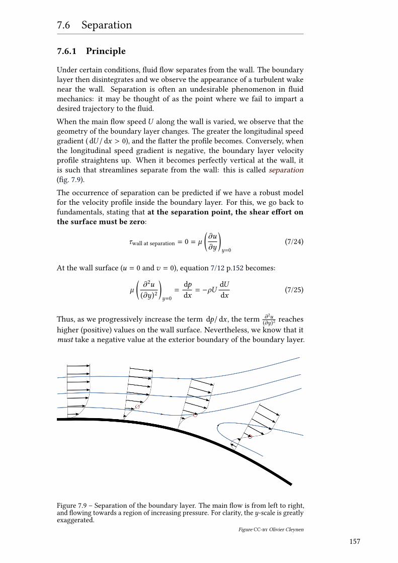
When the main Wow speed U along the wall is varied, we observe that thegeometry of the boundary layer changes. The greater the longitudinal speedgradient ( dU / dx > 0), and the Watter the proVle becomes. Conversely, whenthe longitudinal speed gradient is negative, the boundary layer velocityproVle straightens up. When it becomes perfectly vertical at the wall, itis such that streamlines separate from the wall: this is called separation(Vg. 7.9).

The occurrence of separation can be predicted if we have a robust modelfor the velocity proVle inside the boundary layer. For this, we go back tofundamentals, stating that at the separation point, the shear eUort onthe surface must be zero:

τwall at separation = 0 = µ(∂u

∂y

)y=0

(7/24)

At the wall surface (u = 0 and v = 0), equation 7/12 p.152 becomes:

µ

(∂2u

(∂y)2

)y=0=

dpdx= −ρU

dUdx

(7/25)

Thus, as we progressively increase the term dp/ dx , the term ∂2u(∂y)2

reacheshigher (positive) values on the wall surface. Nevertheless, we know that itmust take a negative value at the exterior boundary of the boundary layer.

Figure 7.9 – Separation of the boundary layer. The main Wow is from left to right,and Wowing towards a region of increasing pressure. For clarity, the y-scale is greatlyexaggerated.

Figure CC-by Olivier Cleynen

157

Therefore, it must change sign somewhere in the boundary. This point where∂2u(∂y)2

changes sign is called inWexion point.

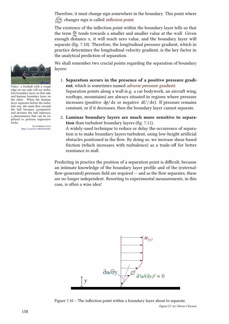
The existence of the inWection point within the boundary layer tells us thatthe term ∂u

∂y tends towards a smaller and smaller value at the wall. Givenenough distance x , it will reach zero value, and the boundary layer willseparate (Vg. 7.10). Therefore, the longitudinal pressure gradient, which inpractice determines the longitudinal velocity gradient, is the key factor inthe analytical prediction of separation.

Video: a football with a roughedge on one side will see turbu-lent boundary layer on that sideand laminar boundary layer onthe other. When the laminarlayer separates before the turbu-lent one, the main Wow aroundthe ball becomes asymmetricand deviates the ball sideways,a phenomenon that can be ex-ploited to perform impressivetricks.

by freekikerz (styl)https://youtu.be/rzRuZNvkMbc

We shall remember two crucial points regarding the separation of boundarylayers:

1. Separation occurs in the presence of a positive pressure gradi-ent, which is sometimes named adverse pressure gradient.Separation points along a wall (e.g. a car bodywork, an aircraft wing,rooftops, mountains) are always situated in regions where pressureincreases (positive dp/ dx or negative dU / dx). If pressure remainsconstant, or if it decreases, then the boundary layer cannot separate.

2. Laminar boundary layers are much more sensitive to separa-tion than turbulent boundary layers (Vg. 7.11).A widely-used technique to reduce or delay the occurrence of separa-tion is to make boundary layers turbulent, using low-height artiVcialobstacles positioned in the Wow. By doing so, we increase shear-basedfriction (which increases with turbulence) as a trade-oU for betterresistance to stall.

Predicting in practice the position of a separation point is diXcult, becausean intimate knowledge of the boundary layer proVle and of the (external-Wow-generated) pressure Veld are required — and as the Wow separates, theseare no longer independent. Resorting to experimental measurements, in thiscase, is often a wise idea!

Figure 7.10 – The inWection point within a boundary layer about to separate.Figure CC-by Olivier Cleynen

158

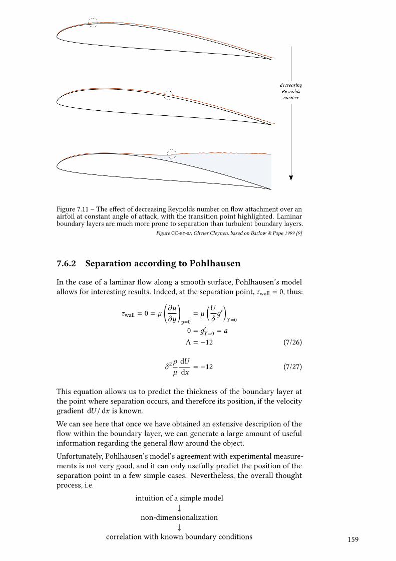
Figure 7.11 – The eUect of decreasing Reynolds number on Wow attachment over anairfoil at constant angle of attack, with the transition point highlighted. Laminarboundary layers are much more prone to separation than turbulent boundary layers.

Figure CC-by-sa Olivier Cleynen, based on Barlow & Pope 1999 [9]

7.6.2 Separation according to Pohlhausen

In the case of a laminar Wow along a smooth surface, Pohlhausen’s modelallows for interesting results. Indeed, at the separation point, τwall = 0, thus:

τwall = 0 = µ(∂u

∂y

)y=0= µ

(Uδд′

)Y=0

0 = д′Y=0 = a

Λ = −12 (7/26)

δ 2ρ

µ

dUdx= −12 (7/27)

This equation allows us to predict the thickness of the boundary layer atthe point where separation occurs, and therefore its position, if the velocitygradient dU / dx is known.

We can see here that once we have obtained an extensive description of theWow within the boundary layer, we can generate a large amount of usefulinformation regarding the general Wow around the object.

Unfortunately, Pohlhausen’s model’s agreement with experimental measure-ments is not very good, and it can only usefully predict the position of theseparation point in a few simple cases. Nevertheless, the overall thoughtprocess, i.e.

intuition of a simple model↓

non-dimensionalization↓

correlation with known boundary conditions 159

↓

exploitation of the model to predict Wow behavior

is what should be remembered here, for it is typical of the research processin Wuid dynamics.

160