Embed Size (px)
Citation preview

Fluid MechanicsChapter 3 – Analysis of existing Wows
last edited September 23, 2017
3.1 Motivation 613.2 The Reynolds transport theorem 61
3.2.1 Control volume 613.2.2 Rate of change of an additive property 61Rate of change of an additive property 62
3.3 Mass conservation 643.4 Change of linear momentum 653.5 Change of angular momentum 673.6 Energy conservation 683.7 The Bernoulli equation 693.8 Limits of integral analysis 713.9 Exercises 73
These lecture notes are based on textbooks by White [13], Çengel & al.[16], and Munson & al.[18].
3.1 Motivation
Video: pre-lecture brieVng forthis chapter, part 1/2
by o.c. (CC-by)https://youtu.be/1LXlFVtPoCY
Our objective for this chapter is to answer the question “what is the net eUectof a given Wuid Wow through a given volume?”.
Here, we develop a mass, momentum and energy accounting methodology toanalyze the Wow of continuous medium. This method is not powerful enoughto allow us to describe extensively the nature of Wuid Wow around bodies;nevertheless, it is extremely useful to quantify forces, moments, and energytransfers associated with Wuid Wow.
3.2 The Reynolds transport theorem
3.2.1 Control volume
Let us begin by describing the Wow which interests us a a generic velocityVeld ~V = (u,v,w ) which is a function of space and time (~V = f (x ,y,z,t )).
Within this Wow, we are interested in an arbitrary volume named controlvolume (CV) which is free to move and change shape (Vg. 3.1). We are goingto measure the properties of the Wuid at the borders of this volume, whichwe call the control surface (CS), in order to compute the net eUect of the Wowthrough the volume.
At a given time, the control volume contains a certain amount of mass whichwe call the system (sys). Thus the system is a Vxed amount of mass transitingthrough the control volume at the time of our study, and its properties(volume, pressure, velocity etc.) may change in the process.
All along the chapter, we are focusing on the question: based on measuredWuid properties at some point in space and time (the properties at the controlsurface), how can we quantify what is happening to the system (the massinside the control volume)?
61

Figure 3.1 – A control volume within a Wow. The system is the amount of massincluded within the control volume at a given time. At a later time, it may have leftthe control volume, and its shape and properties may have changed. The controlvolume may also change shape with time, although this is not represented here.
Figure CC-0 o.c.
3.2.2 Rate of change of an additive property
In order to proceed with our calculations, we need a robust accountingmethodology. We start with a “dummy” Wuid property B, which we will laterreplace with physical variables of interest.Let us thus consider an arbitrary additive property B of the Wuid. By the termadditive property, we mean that the total amount of property is divided if theWuid is divided. For instance, this is true of mass, volume, energy, entropy,but not pressure or temperature.The speciVc (i.e. per unit mass) value of B is designated b ≡ B/m.
We now wish to compute the variation of a system’s property B based onmeasurements made at the borders of the control volume. We will achievethis with an equation containing three terms:
• The time variation of the quantity B within the system is measuredwith the term
dBsys
dt . This may represent, for example, the rate of changeof the Wuid’s internal energy as it travels through a jet engine.
• Within the control volume, the enclosed quantity BCV can vary byaccumulation (for example, mass may be increasing in an air tank fedwith compressed air): we measure this with the term dBCV
dt .
• Finally, a mass Wux may be Wowing through the boundaries of thecontrol volume, carrying with it some amount of B every second: wename that net Wow out of the system Bnet ≡ Bout − Bin.
62

We can now link these three terms with the simple equation:
dBsys
dt=
dBCV
dt+ Bnet (3/1)
the rate of change
of B for the system=
the rate of change
of B within the
control volume
+
the net Wow of B
through the boundaries
of the control volume
Since B may not be uniformly distributed within the control volume, we liketo express the term dBCV
dt as the integral of the volume density BV
with respectto volume:
dBCV
dt=
ddt
$CV
B
VdV =
ddt
$CVρb dV (3/2)
Obtaining a value for this integral may be diXcult, especially if the volumeof the control volume CV is itself a function of time.
The term Bnet can be evaluated by quantifying, for each area element dA ofthe control volume’s surface, the surface Wow rate ρbV⊥ of property B thatWows through it (Vg. 3.2). The integral over the entire control volume surfaceCS of this term is:
Bnet =
"CSρbV⊥ dA =
"CSρb (~Vrel · ~n) dA (3/3)
where Wows and velocities are positive outwards and negative inwards by convention,CV is the control volume,CS is the the control surface (enclosing the control volume),~n is a unit vector on each surface element dA pointing outwards,~Vrel is the local velocity of Wuid relative to the control surface,
and V⊥ ≡ ~Vrel · ~n is the local cross-surface speed.
By inserting equations 3/2 and 3/3 into equation 3/1, we obtain:
Figure 3.2 – Part of the system may be Wowing through an arbitrary piece of thecontrol surface with area dA. The ~n vector deVnes the orientation of dA surface,and by convention is always pointed outwards.
Figure CC-0 o.c.
63

dBsys
dt=
ddt
$CVρb dV +
"CSρb (~Vrel · ~n) dA (3/4)
Equation 3/4 is named the Reynolds’ transport theorem; it stands now as ageneral, abstract accounting tool, but as we soon replace B by meaningfulvariables, it will prove extremely useful, allowing us to quantify the net eUectof the Wow of a system through a volume for which border properties areknown.
In the following sections we are going to use this equation to assert four keyphysical principles (§0.7) in order to analyze the Wow of Wuids:
• mass conservation;
• change of linear momentum;
• change of angular momentum;
• energy conservation.
3.3 Mass conservation
Video: with suXcient skills (andlots of practice!), it is possiblefor a musician to produce an un-interrupted stream of air intoan instrument while still con-tinuing to breathe, a techniquecalled circular breathing. Canyou identify the diUerent termsof eq. 3/5 as they apply to theclarinetist’s mouth?
by David Hernando Vitores (CC-by-sa)https://frama.link/yVesHaSk
In this section, we focus on simply asserting that mass is conserved (eq. 0/22p.19). Our study of the Wuid’s properties at the borders of the control volumeis made by replacing variable B by mass m. Thus dB
dt becomesdmsys
dt , whichby deVnition is zero.In a similar fashion, b ≡ B/m =m/m = 1 and consequently the Reynoldstransport theorem (3/4) becomes:
dmsys
dt= 0 =
ddt
$CVρ dV +
"CSρ (~Vrel · ~n) dA (3/5)
the time change
of the system’s mass= 0 =
the rate of change
of mass inside
the control volume
+
the net mass Wow
at the borders
of the control volume
This equation 3/5 is often called continuity equation. It allows us to comparethe incoming and outgoing mass Wows through the borders of the controlvolume.
When the control volume has well-deVned inlets and outlets through whichthe term ρ (~Vrel · ~n) can be considered uniform (as for example in Vg. 3.3), thisequation reduces to:
0 =ddt
$CVρ dV +
∑out
{ρV⊥A
}+
∑in
{ρV⊥A
}(3/6)
=ddt
$CVρ dV +
∑out
{ρ |V⊥ |A
}−
∑in
{ρ |V⊥ |A
}=
ddt
$CVρ dV +
∑out
{m} −∑in
{m} (3/7)
In equation 3/6, the term ρV⊥A at each inlet or outlet corresponds to the localmass Wow ±m (positive inwards, negative outwards) through the boundary.
64

Figure 3.3 – A control volume for which the system’s properties are uniform ateach inlet and outlet. Here eq. 3/5 translates as 0 = d
dt
#CV ρ dV + ρ3 |V⊥3 |A3 +
ρ2 |V⊥2 |A2 − ρ1 |V⊥1 |A1.Figure CC-0 o.c.
With equation 3/7 we can see that when the Wow is steady (§0.8), the last twoterms amount to zero, and the integral
#CV ρ dV (the total amount of mass
in the control volume) does not change with time.
3.4 Change of linear momentum
In this section, we apply Newton’s second law: we assert that the variationof system’s linear momentum is equal to the net force being applied to it(eq. 0/23 p.19). Our study of the Wuid’s properties at the control surface iscarried out by replacing variable B by the quantity m~V : momentum. Thus,dBsys
dt becomesd(m~Vsys)
dt , which is equal to ~Fnet, the vector sum of forces appliedon the system as it transits the control volume.In a similar fashion, b ≡ B/m = ~V and equation 3/4, the Reynolds transporttheorem, becomes:
d(m~Vsys )
dt= ~Fnet =
ddt
$CVρ~V dV +
"CSρ~V (~Vrel · ~n) dA
(3/8)
the vector sum of
forces on the system=
the rate of change
of linear momentum
within the control volume
+
the net Wow of linear momen-
tum through the boundaries
of the control volume
When the control volume has well-deVned inlets and outlets through whichthe term ρ~V (~Vrel ·~n) can be considered uniform (Vg. 3.3), this equation reducesto:
~Fnet =ddt
$CVρ~V dV +
∑out
{(ρ |V⊥ |A)~V
}−
∑in
{(ρ |V⊥ |A)~V
}(3/9)
=ddt
$CVρ~V dV +
∑out
{m~V
}−
∑in
{m~V
}(3/10)
65
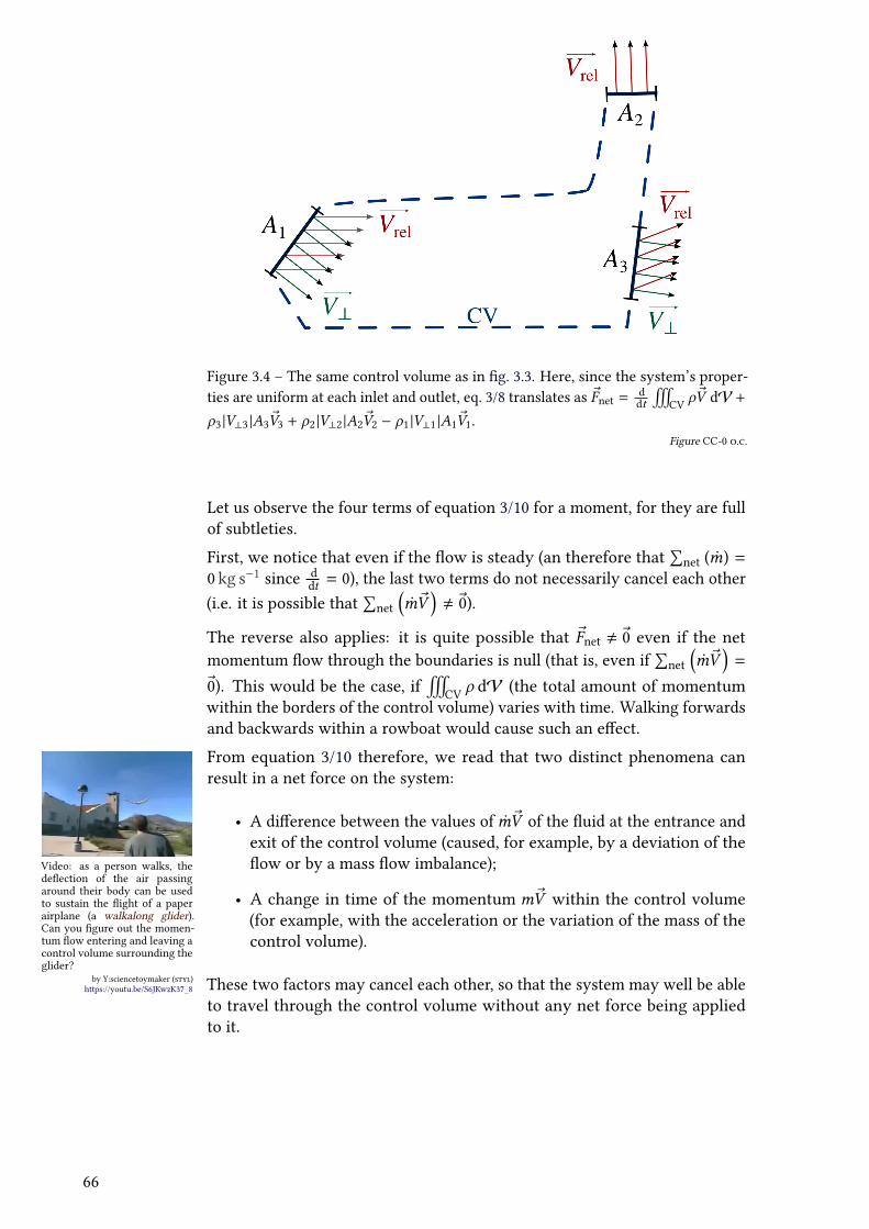
Figure 3.4 – The same control volume as in Vg. 3.3. Here, since the system’s proper-ties are uniform at each inlet and outlet, eq. 3/8 translates as ~Fnet =
ddt
#CV ρ
~V dV +
ρ3 |V⊥3 |A3~V3 + ρ2 |V⊥2 |A2~V2 − ρ1 |V⊥1 |A1~V1.Figure CC-0 o.c.
Let us observe the four terms of equation 3/10 for a moment, for they are fullof subtleties.
First, we notice that even if the Wow is steady (an therefore that∑
net (m) =0 kg s−1 since d
dt = 0), the last two terms do not necessarily cancel each other(i.e. it is possible that
∑net
(m~V
), ~0).
The reverse also applies: it is quite possible that ~Fnet , ~0 even if the netmomentum Wow through the boundaries is null (that is, even if
∑net
(m~V
)=
~0). This would be the case, if#
CV ρ dV (the total amount of momentumwithin the borders of the control volume) varies with time. Walking forwardsand backwards within a rowboat would cause such an eUect.
Video: as a person walks, thedeWection of the air passingaround their body can be usedto sustain the Wight of a paperairplane (a walkalong glider).Can you Vgure out the momen-tum Wow entering and leaving acontrol volume surrounding theglider?
by Y:sciencetoymaker (styl)https://youtu.be/S6JKwzK37_8
From equation 3/10 therefore, we read that two distinct phenomena canresult in a net force on the system:
• A diUerence between the values of m~V of the Wuid at the entrance andexit of the control volume (caused, for example, by a deviation of theWow or by a mass Wow imbalance);
• A change in time of the momentum m~V within the control volume(for example, with the acceleration or the variation of the mass of thecontrol volume).
These two factors may cancel each other, so that the system may well be ableto travel through the control volume without any net force being appliedto it.
66

3.5 Change of angular momentum
Video: pre-lecture brieVng forthis chapter, part 2/2
by o.c. (CC-by)https://youtu.be/nmEe7Dq01AU
In this third spin on the Reynolds transport theorem, we assert that thechange of the angular momentum of a system about a point X is equal tothe net moment applied on the system about this point (eq. 0/24 p.19). Ourstudy of the Wuid’s properties at the borders of the control volume is madeby replacing the variable B by the angular momentum ~rXm ∧ m~V . Thus,dBsys
dt becomesd(~rXm∧m~Vsys)
dt , which is equal to ~Mnet, the vector sum of momentsapplied on the system about point X as it transits through the control volume.
In a similar fashion, b ≡ B/m = ~r∧~V and equation 3/4, the Reynolds transporttheorem, becomes:
d(~rXm ∧m~V )sys
dt= ~Mnet,X =
ddt
$CV
~rXm ∧ ρ~V dV+"
CS~rXm ∧ ρ (~Vrel · ~n)~V dA
(3/11)the sum of
moments applied
to the system
=
the rate of change of
the angular momentum
in the control volume
+
the net Wow of angular
momentum through the
control volume’s boundaries
in which ~rXm is a vector giving the position of any massm relative to point X .
Video: rocket landing gonewrong. Can you compute themoment exerted by the topthruster around the base of therocket as it (unsuccessfully) at-tempts to compensate for thecollapsed landing leg?
by Y:SciNews (styl)https://youtu.be/4cvGGxTsQx0
When the control volume has well-deVned inlets and outlets through whichthe term ~rXm ∧ ρ (~Vrel · ~n)~V can be considered uniform (Vg. 3.5), this equationreduces to:
~Mnet,X =ddt
$CV
~rXm ∧ ρ~V dV +∑out
{~rXm ∧ m~V
}−
∑in
{~rXm ∧ m~V
}
(3/12)
Figure 3.5 – A control volume for which the properties of the system are uniformat each inlet or outlet. Here the moment about point X is ~Mnet,X ≈
ddt
#CV
~rXm ∧
ρ~V dV + ~r2 ∧ |m2 |~V2 − ~r1 ∧ |m1 |~V1.Figure CC-0 o.c.
Equation 3/12 allows us to quantify, with relative ease, the moment exertedon a system based on inlet and outlet velocities of a control volume.
67

3.6 Energy conservation
We conclude our frantic exploration of control volume analysis with the Vrstprinciple of thermodynamics. We now simply assert that the change in theenergy of a system can only be due to well-identiVed transfers (eq. 0/25 p.19).Our study of the Wuid’s properties at the borders of the control volume ismade by replacing variable B by an amount of energy Esys. Now,
dEsys
dt can beattributed to three contributors:
dEsys
dt= Qnet in + Wshaft, net in + Wpressure, net in (3/13)
where Qnet in is the net power transfered as heat;Wshaft, net in is the net power added as work with a shaft;
and Wpressure, net in is the net power required to enter and leave the control volume.
It follows that b ≡ B/m = E/m ≡ e; and e is broken down into
e = i + ek + ep (3/14)
where i is the speciVc internal energy (J kg−1);ek the speciVc kinetic energy (J kg−1);
and ep the speciVc potential energy (J kg−1).
Now, the Reynolds transport theorem (equation 3/4) becomes:
dEsys
dt= Qnet in + Wshaft, net in + Wpressure, net in =
ddt
$CVρ e dV +
"CSρ e (~Vrel · ~n) dA
(3/15)
When the control volume has well-deVned inlets and outlets through whichthe term ρ e (~Vrel · ~n) can be considered uniform, this equation reduces to:
Qnet in + Wshaft, net in + Wpressure, net in =ddt
$CVρ e dV +
∑out
{m e} −∑in
{m e} (3/16)
Qnetin + Wshaft, net in =ddt
$CVρ e dV +
∑out
{m(i + ek + ep )
}
−∑in
{m(i + ek + ep )
}− Wpressure, net in
=ddt
$CVρ e dV +
∑out
{m
(i +
12V 2 + дz
)}−
∑in
{m
(i +
12V 2 + дz
)}+
∑out
{mp
ρ
}−
∑in
{mp
ρ
}
Making use of the concept of enthalpy deVned as h ≡ i + p/ρ, we obtain:
Qnet in + Wshaft, net in =ddt
$CVρ e dV +
∑out
{m
(h +
12V 2 + дz
)}−
∑in
{m
(h +
12V 2 + дz
)}(3/17)
the net power
received by the system=
the rate of change
of energy inside
the control volume
+the net energy Wow rate
exiting the control volume boundaries68

This equation 3/17 is particularly attractive, but it necessitates the input ofa large amount of experimental data to provide useful results. It is indeedvery diXcult to predict how the terms i and p/ρ will change for a given Wowprocess. For example, a pump with given power Qnet in and Wshaft, net in willgenerate large increases of terms p,V and z if it is eXcient, or a large increaseof terms i and 1/ρ if it is ineXcient. This equation 3/17, sadly, does not allowus to quantify the net eUect of shear and the extent of irreversibilities in aWuid Wow.
3.7 The Bernoulli equation
The Bernoulli equation has very little practical use for us; nevertheless it isso widely used that we have to dedicate a brief section to examining it. Wewill start from equation 3/17 and add Vve constraints:
1. Steady Wow.Thus d
dt
#CV ρ e dV = 0.
In addition, m has the same value at inlet and outlet;
2. Incompressible Wow.Thus, ρ stays constant;
3. No heat or work transfer.Thus, both Qnet in and Wshaft, net in are zero;
4. No friction.Thus, the Wuid energy i cannot increase due to an input from thecontrol volume;
5. One-dimensional Wow.Thus, our control volume has only one known entry and one knownexit, all Wuid particles move together with the same transit time, andthe overall trajectory is already known.
With these Vve restrictions, equation 3/17 simply becomes:
0 =∑out
{m(i +
p
ρ+ ek + ep )
}−
∑in
{m(i +
p
ρ+ ek + ep )
}= m
[(i +
p2
ρ+
12V 2
2 + дz2) − (i +p1
ρ+
12V 2
1 + дz1)
]
and we here obtain the Bernoulli equation:
p1
ρ+
12V 2
1 + дz1 =p2
ρ+
12V 2
2 + дz2 (3/18)
This equation describes the properties of a Wuid particle in a steady, incom-pressible, friction-less Wow with no energy transfer.
The Bernoulli equation can also be obtained starting from the linear momen-tum equation (eq. 3/8 p.65):
~Fnet =ddt
$CVρ~V dV +
"CSρ~V (~Vrel · ~n) dA
69

When considering a Vxed, inVnitely short control volume along a knownstreamline s of the Wow, this equation becomes:
d~Fpressure + d~Fshear + d~Fgravity =ddt
$CVρ~V dV + ρVAd~V
along a streamline, where the velocity ~V is aligned (by deVnition) with the streamline.
Now, adding the restrictions of steady Wow ( d/ dt = 0) and no friction( d~Fshear = ~0), we already obtain:
d~Fpressure + d~Fgravity = ρVAd~V
The projection of the net force due to gravity d~Fgravity on the streamlinesegment ds has norm d~Fgravity · d~s = −дρAdz, while the net force due topressure is aligned with the streamline and has norm dFpressure,s = −Adp.Along this streamline, we thus have the following scalar equation, which weintegrate from points 1 to 2:
−Adp − ρдAdz = ρVAdV
−1ρ
dp − д dz = V dV
−
∫ 2
1
1ρ
dp −∫ 2
1д dz =
∫ 2
1V dV
The last obstacle is removed when we consider Wows without heat or worktransfer, where, therefore, the density ρ is constant. In this way, we arrive toequation. 3/18 again:
p1
ρ+
12V 2
1 + дz1 =p2
ρ+
12V 2
2 + дz2
Let us insist on the incredibly frustrating restrictions brought by the Vveconditions above:
1. Steady Wow.This constrains us to continuous Wows with no transition eUects, whichis a reasonable limit;
2. Incompressible Wow.We cannot use this equation to describe Wow in compressors, turbines,diUusers, nozzles, nor in Wows where M > 0,6.
3. No heat or work transfer.We cannot use this equation in a machine (e.g. in pumps, turbines,combustion chambers, coolers).
4. No friction.This is a tragic restriction! We cannot use this equation to describe aturbulent or viscous Wow, e.g. near a wall or in a wake.
5. One-dimensional Wow.This equation is only valid if we know precisely the trajectory of theWuid whose properties are being calculated.
Among these, the last is the most severe (and the most often forgotten):the Bernoulli equation does not allow us to predict the trajectory ofWuid particles. Just like all of the other equations in this chapter, it requiresa control volume with a known inlet and a known outlet.70

3.8 Limits of integral analysis
Integral analysis is an incredibly useful tool in Wuid dynamics: in any givenproblem, it allows us to rapidly describe and calculate the main Wuid phenom-ena at hand. The net force exerted on the Wuid as it is deWected downwardsby a helicopter, for example, can be calculated using just a loosely-drawncontrol volume and a single vector equation.
As we progress through exercise sheet 3, however, the limits of this methodslowly become apparent. They are twofold.
• First, we are conVned to calculating the net eUect of Wuid Wow. The netforce, for example, encompasses the integral eUect of all forces —due topressure, shear, and gravity— applied on the Wuid as it transits throughthe control volume. Integral analysis gives us absolutely no way ofdistinguishing between those sub-components. In order to do that (forexample, to calculate which part of a pump’s mechanical power is lostto internal viscous eUects), we would need to look within the controlvolume.
• Second, all four of our equations in this chapter only work in onedirection. The value dBsys/ dt of any Vnite integral cannot be used toVnd which function ρbV⊥ dA was integrated over the control surface toobtain it. For example, there are an inVnite number of velocity proVleswhich will result in a net force of −12 N. Knowing the net value of anintegral, we cannot deduce the conditions which lead to it.In practice, this is a major limitation on the use of integral analysis,because it conVnes us to working with large swaths of experimentaldata gathered at the borders of our control volumes. From the wakebelow the helicopter, we deduce the net force; but the net force tells usnothing about the shape of the wake.
Clearly, in order to overcome these limitations, we are going to need to openup the control volume, and look at the details of the Wow within — perhapsby dividing it into a myriad of sub-control volumes. This is what we setourselves to in chapter 4, with a thundering and formidable methodology weshall call derivative analysis.
71

72