Fluid lipid membranes – a primer

Markus DesernoMax-Planck-Institut fur PolymerforschungAckermannweg 10, 55128 Mainz, Germany

Contents

1 Self assembly 11.1 Lipids . . . . . . . . . . . . . . . . . . . . . . . . . . . . . . . . . . . . . . . . . 21.2 The morphology of surfactant aggregates . . . . . . . . . . . . .. . . . . . . . . 3

2 Membrane elasticity 72.1 Stretching and shearing . . . . . . . . . . . . . . . . . . . . . . . . . . .. . . . . 72.2 Bending . . . . . . . . . . . . . . . . . . . . . . . . . . . . . . . . . . . . . . . . 8

3 Surface curvature 123.1 Directional curvature and principal curvatures . . . . . .. . . . . . . . . . . . . . 123.2 Monge parametrization . . . . . . . . . . . . . . . . . . . . . . . . . . . .. . . . 14

4 Helfrich theory 144.1 The Helfrich Hamiltonian . . . . . . . . . . . . . . . . . . . . . . . . . .. . . . . 154.2 The shape equation of linear theory . . . . . . . . . . . . . . . . . .. . . . . . . . 17

4.2.1 Variation of the energy functional . . . . . . . . . . . . . . . .. . . . . . 174.2.2 Boundary conditions . . . . . . . . . . . . . . . . . . . . . . . . . . . .. 194.2.3 A few worked out examples . . . . . . . . . . . . . . . . . . . . . . . . .194.2.4 Nonlinear shape equation . . . . . . . . . . . . . . . . . . . . . . . .. . . 26

4.3 Membrane fluctuations . . . . . . . . . . . . . . . . . . . . . . . . . . . . .. . . 26

1 Self assembly

Lipid membranes are quasi-two-dimensional structures which form by spontaneous aggregation oflipid molecules in aqueous solution. Such a process is an example of what is termedself-assembly.It can be found frequently in nature, whenever a large numberof molecules form a condensedaggregate of some nontrivial structure, driven by the possibility to lower the free energy in doingso. Strictly speaking, even the formation of a sodium-chloride crystal may thus be viewed as aself-assembly process, but the terminology is usually restricted to cases in which supramolecularaggregates of somewhat more complicated structure are being formed – in particular, when due to

1

Box 1 (Hydrophobic effect)The insertion of a molecule into water occurs spontaneously when it leads to a lowering of theoverall free energy. Recall that this involves not only the question whether there exists a favorableinteraction energy (say, of van der Waals or electrostatic type), but also whether the processis entropically favorable. Liquid water has a great deal of entropy, related to the translationalor rotational degrees of freedom of water. However, particularly the latter are restricted by thefact that water just loves to form hydrogen bonds with itself, i. e., point an H-atom of one H2Omolecule towards the O-atom of another. The resulting network of hydrogen bonds is a delicatebalance between energy and entropy, and the insertion of other molecules might locally disturbthis network, thereby also influencing the water entropy. A good rule of thumb is that if a moleculeis also able to efficiently take part in hydrogen bonding (such as glucose or sucrose), it will tend todissolve easier than a molecule which is unable to do this (such as oil). Generally, polar molecules(i. e., molecules with local electrical dipole moments) blend more readily into the hydrogen bondnetwork. Around the very non-polar surface of a hydrocarbon chain water molecules can onlyform hydrogen bonds with themselves, but since these molecules have fewer neighbors, they havefewer possibilities to do so, leading thereby to lower entropy in the water layer adjacent to a non-polar surface, which in turn works against solubilization. What may sound intuitively appealing,is in fact much more complicated and remains partially disputed even today. The difficulty is thatcertain energy-entropy compensation effects make it impossible to “attribute” certain effects in anunambiguous way to either energy or entropy. The interested reader will find some useful materialin Refs. [10, 18, 22, 23].

the aggregation process entities appear which are characterized by the emergence of new lengthscales. Self-assembly is thus a classical route by which hierarchically structured materials form,and it is thus of great interest to physicists and engineers alike. And since Nature has the well-deserved reputation of having engineered the best machinesliterally walking this planet, self-assembly is indeed one of its close allies, and it is thus of great interest for biologists, too. Fluidlipid bilayers of course belong to the class of systems whichhold an obvious biological relevance.In this introductory section we first want to familiarize ourselves a bit with some of the idiosyn-crasies of lipid self assembly, before we turn to propertiesof the structures which form in thisprocess – lipid membranes.

1.1 Lipids

Lipids are Nature’s sophisticated version of surfactants.They are amphiphilic molecules whichconsist of one part, called thehead, which is hydrophilic – “in love with water”, and another part,termedtail, which is hydrophobic – “afraid of water”. Whether a molecular structure or a partof it likes or dislikes water depends on its detailed chemical buildup, and it is closely related tothe question of whether this structure could be solubilizedin water. Sugar for instance dissolvesreadily in water, oil doesn’t — see also Box 1Lipids come in many different kinds in nature, and this is notthe place to classify them (the readerwill find a bit more detail in Ref. [16, Chap. 1]. I only want to say a bit more about the mostcommon ones – glycerophospholipids. Their hydrophobic part consists of (normally) two simplehydrocarbon chains, having a (typically even) number of C-atoms (typically between 12 and 24)and maybe some (typically cis-) double bonds. These chains previously belonged to the corre-sponding fatty acid, for instance palmitic acid, and two such chains are linked via ester bonds

2

to two of the OH groups of a molecule of glycerol. Its third OH group is esterified to a phos-phate group, which carries the terminal head group of the lipid, for which again there exist manypossibilities, for instance a choline group. A sophisticated (and partly intimidating) terminologyhas been developed to communicate the relevant details of this architecture. For instance, palmi-toyloleoylphosphatidylcholine – abbreviated POPC – is a lipid which has one hydrocarbon chainderived from palmitic acid (a saturated fatty acid with 16 carbons and no double bond), anotherchain coming from oleic acid (an unsaturated fatty acid withone cis double bond at position 9 and18 carbons), and a phosphate link to a choline group. Or dimyristoylphosphatidylserine – abbre-viated DMPS – has two chains stemming from myristic acid (a saturated fatty acid with 14 carbonatoms and no double bond) – linked again via a phosphate to theamino acid serine. Some more onstructure and naming conventions can be found in the Boxes 2 and 3. As physicists we can permitourselves to neglect much of the detail, but some key points are worth paying attention to:

• The length of the fatty acids. The longer they are, the more hydrophobic is the lipid (and thethicker will the membrane be later).

• Are there double bonds? If yes, the tails tend to be more disordered, and this increases thefluidity of the forming membranes (more precisely, it increases the temperature of the “maintransition” between “fluid” and “gel” phase) [16, Chap. 5].

• Is the head group charged? Note that the phosphate itself already carries one negative charge.For neutral lipids the group attached to the phosphate must thus carry a positive countercharge (as choline does, but for instance not serine).

1.2 The morphology of surfactant aggregates

The hydrophobic parts of amphiphilic molecules do not like to dissolve in water. But what if theyhave to, because we put them in water anyways? The trick is that they can develop a coopera-tive strategy in which many of them combine to an aggregate which shields its hydrophobic partagainst the surrounding water by using the hydrophilic part. Morphologically such aggregates canfor instance be spheres, with all the tails in the inside and the heads on the surface. Such objects arecalled (spherical) “micelles” (from the Latin word “mica”,grain). One could also imagine cylin-drical aggregates with the hydrophobic tails in the inside and the heads again on the surface; theseare called cylindrical or wormlike micelles. And finally onecan also imagine a double-layer inwhich the hydrophobic tails are sandwiched between two planes of hydrophilic head groups. Thisis the lipid bilayer membrane that will keep us busy later. But before we look at it in any greaterdetail, we would like to understand what aspect of the amphiphile determines the morphology thatis spontaneously being formed.Possibly the simplest answer to this question has been givenby Israelachvili, Mitchell, and Ninhamin a famous paper from 1976, and it is a wonderful example of a simple geometry argument [13].Here’s how it goes: Assume that the particular amphiphilic molecule has a head that needs an areaa inside an aggregate, and that it has a volumev and a tail lengthℓ. Let’s try to form a sphericalaggregate of radiusR out of N such molecules. Of course, we then must have4πR2 = Na and43πR3 = Nv. By forming the ratio of these two equations the aggregate numberN drops out and

we find for the radius

Rsphere=3v

a. (1)

3

Box

2(Lipid

structureand

head-groups)

3

CH3

CH3

CH

+N C C

+N C C

+

CCC

O

O

N

_OH CCC

OHOH

CCC

CC

COH

OH

HO

HO 1

23

4

56

esterbond

esterbond

phosphatebondester

O

O

O

O

OP

O

O

O_

H

1

negative charge!

2 4 6 8 11 13 15 17

18161412109753

cis

12

3

4

5

6

7

8

9

10

11

12

13

14

15

16Palmitoyl

Oleoyl

head groupglycerol

phosphate

esterbond

H O2

esterification

C

C

C

H

H

H

H

H

O

O

O

H

H

C

O+

C

C

C

H

H

H

H

H

O

O

O

H

H

H

OH

C

O

glycerol

fatty acid

positively charged neutral

unsaturated fatty acid

Example: 1−Palmitoyl−2−Oleoyl−sn−Glycero−3−Phosphocholine (POPC)

phosphatidylcholin = "Lecithin"

choline ethanolamine serine glycerol inositol(amino acid) (cyclitol)(alcohol)(amine) (amine)

(OH) (OH) (OH) (OH)

(OH)

gives negative lipidgives neutral lipid

4

Box

3(N

aming

conventionsfor

simple

fatty-acidlipid-tails)

# carbon saturated 1-fold unsaturated 2-fold unsaturated 4-fold unsaturated 6-fold unsaturated

12 Lauroyl

13 Tridecanoyl

14 MyristoylMyristoleoyl (9-cis)

Myristelaidoyl (9-trans)

15 Pentadecanoyl

16 PalmitoylPalmitoleoyl (9-cis)

Palmitelaidoyl (9-trans)

17 Heptadecanoyl

18 Stearoyl

Petroselinoyl (6-cis)

Oleoyl (9-cis)

Elaidoyl (9-trans)

Linoleoyl ((9,12)-cis)

19 Nonadecanoyl

20 Arachidoyl Eicosenoyl (11-cis) Arachidonoyl ((5,8,11,14)-cis)

21 Heniecosanoyl

22 Behenoyl Erucoyl (13-cis) Docosahexaenoyl ((4,7,10,13,16,19)-cis)

24 Lignoceroyl Nervonoyl (15-cis)

Symmetric Fatty Acid lipids: 1,2-Diacyl-sn-Glycero-3-Phosphocholine

e.g. 1,2-Dipalmitoyl-sn-Glycero-3-Phosphocholine (16:0-PC, DPPC)

Asymmetric Fatty Acid lipids: 1-Acyl-2-Acyl-sn-Glycero-3-Phosphocholine

e.g. 1-Palmitoyl-2-Oleoyl-sn-Glycero-3-Phosphocholine (16:0-18:1-PC, POPC)

This is the "famous"Omega−3 fatty acid

5

a b c d eFigure 1: A sequence of aggregate shapes driven by the aspect ratio of asimplified modelam-phiphile. a) three-dimensional droplet, b) bilayer, c) branched cylindrical micelles, d) unbranchedcylindrical micelles, e) spherical micelles. Taken from Ref. [4].

Since we don’t want to leave a hole in the inner bit of the micelle, the tail length has to be at leastas big as this value,i. e. ℓ ≥ Rsphere, which we can write as

P :=v

ℓa≤ 1

3(spherical aggregates), (2)

where the dimensionless combinationP is referred to as thepacking parameter. This conditionsays that spherical aggregates form if the packing parameter is smaller than1

3.

Let’s repeat the same argument withcylindrical aggregates of (average) lengthL. Let’s assumethat they are long enough such that we can ignore end effects,i. e., L ≫ R. Now,N amphiphilesforming an aggregate have to satisfy the two conditions2πRL = Na andπR2L = Nv, implyingby again taking the ratio

Rcylinder =2v

a. (3)

Since againℓ ≥ Rcylinder must hold, we find that cylinders form ifP ≤ 12. But wait, if P ≤ 1

3we

know that spheres form. This tells us that the proper condition for cylindrical aggregates is

1

3≤ P ≤ 1

2(cylindrical aggregates). (4)

Doing all this again for planar structures, we finally find

1

2≤ P ≤ 1 (planar aggregates). (5)

Notice that the packing parameter essentially tells us something about theaspect ratioof the am-phiphile. A small packing parameter corresponds to “lots ofhead with little tail”, comparable toan ice-cone, where the ball of ice cream is the head and the cone is the tail. Unsurprisingly suchamphiphiles would aggregate into spheres. In contrast, large values of the packing parameter lookmore cylindrical, and it makes sense that such amphiphiles indeed pack in two-dimensional planaraggregates. A sequence of self-assembled aggregate shapesis illustrated in Fig. 1 Notice that lipidstypically look cylindrical – and they owe a fair amount of this property to the fact that they havetwo tails.

6

While the argument sounds irresistibly nice at first sight, it is upon closer inspection not as pre-dictive as it might seem. Suppose you get ambushed by some sinister looking guy in some darkalley at midnight, who forces you at gun-point to tell him thetail volume of, say, DOTAP – whatwould you say? Getting actual numbers in order tocalculateP and thus predict the structure is awhole different question, and it shall not be addressed here. However, it should be pointed out thatthis almost obscenely naive scenario can nevertheless be mapped quantitatively to model lipids forwhich one would never believe that a simplistic ansatz such as this would lead to anything. Thesceptical reader is encouraged to peek into Ref. [4], where it is shown how the sequence fromFig. 1 can be related toP .

2 Membrane elasticity

A physical description of a membrane requires us to know how its energychanges when we dosomething to it. But what can we do that would change the energy? For obvious reasons, overalltranslations and rotations of a piece of bilayer don’t change the energy at all – unless of coursethere exist external (possibly position dependent) fields that couple to the membrane, and we willassume that this is not the case.

2.1 Stretching and shearing

Classical elasticity theory studies energy changes due tostretchingor shearing, so let’s look atsuch deformations, butrestricted to the membrane plane.Stretching does indeed cost energy. Assume that we have a piece of membrane which at zeroexternal stress has an areaA0, and we now stretch it to a sizeA > A0. To lowest order we canwrite the energy change as

Estretch=1

2Kstretch

(A − A0)2

A0, (6)

where the modulusKstretchenters as the proportionality constant between a quadraticdeviation ofthe area from its unstressed state and the respective energy. The additional1/A0 is a convention.1

What is the lateral stress, thetensionΣ, under which the membrane is when we subject it to sucha strain? Per definition, it is the derivative of energy with respect to area:

Σ :=∂Estretch

∂A= Kstretch

A − A0

A0=: Kstretchu , (7)

where we have defined the dimensionlessstrainu = A/A0 − 1. What we have thus recovered isHooke’s law for membrane stretching: Stress is proportional to strain, and the constant of propor-tionality is the stretching modulusKstretch.The stretching modulusKstretch can be measured experimentally, for instance in micropipette ex-periments [8, 19]. There, part of the surface of giant unilamellar vesicles (“lipid-bilayer bubbles inwater”) is being sucked into much smaller micropipettes, such that the vesicle gets under tension.

1How can physics be a convention? Well, we have not yet specified what exactly we mean by the stretching modulus!You could define your own stretching modulusKalternative= Kstretch/A0, and end up with an alternative stretchingenergyEstretch= 1

2Kalternative(A − A0)

2 which of course describes exactly the same physics. However, Eqn. (6) ispreferable for reasons that will become clear in a second.

7

The area change can be measured quite accurately by the amount of membrane which ends upin the micropipette, the tension can be inferred from the vesicle radius and the suction pressure.2

A linear stress-strain relation is indeed confirmed, and forphospholipid membranes one typicallyfinds values ofKstretcharound250 mN/m [19]. Once the membrane stressΣ exceeds a few mN/m,the lipid bilayer suddenly fails and ruptures without much premonition. Using Eqn. (7) we seethat the corresponding rupture strain is only of the order ofa few percent. So, in that respectmembranes are not particularly stretchable.What about shear? In order to have a relation analogous to Eqn. (7) relating a shear stress with ashear strain, the membrane would of course need to be able to support a shear strain in the firstplace. However, the fluid lipid bilayers which we will be concerned with here are unable to do this,preciselybecausethey are fluid. For the same reason that water does not have a shear modulus,fluid lipid membranes don’t.3 Hence, static shear is no deformation which costs a fluid membraneenergy; in fact, it cannot even bedefined.

2.2 Bending

In a three-dimensional chunk of material small elastic stresses always give rise to smallover-all deformations of the material. This is markedly different ifthe material is not ‘really” three-dimensional, because it is “thin” in one direction (a plate)or even two directions (a rod). Platesand rods can bebent in the directions away from the dimension in which they are extended, andthese deformations lead to substantial overall changes in material shape without requiring exces-sive stresses. We have seen this already for polymers in the context of the wormlike-chain model.The same is true for membranes. On sufficiently large length scales membranes can be consideredas essentially two-dimensional surfaces that can be bent into the third dimension.Characteristically, weak bending is a deformation which costs significantly less energy than stretch-ing. Think of a sheet of paper. Its stretching modulus is extremely high, so you will have a hardtime rupturing it bystretchingrather thantearing.4 Yet, bendingis something that we can do veryeasily, because the concomitant local volume strain is verysmall. Let’s see how this works outquantitatively. (The subsequent calculation is a bit simplified, in particular since it neglects issuessuch as the Poisson ratio, which is defined in Box. 4. The reader will find a more careful treatmentin Ref. [15].)Take a quadratic sheet of paper of side lengthL and curve it in one direction such that it has aradius of curvatureR (see Fig. 2). The outside of the paper is stretched a little bit, while the insideis compressed a little bit. In the middle of the paper will be aregion which is not strained at all, theso calledneutral surface. What is the total stretching energy? If we assume thatlocally the papermaterial follows a simple elastic relation in analogy to Eqn. (6), namely

Estretch=1

2Y

(V − V0)2

V0

(three dimensions, uniaxial extension), (9)

2A spherical surface of radiusR and surface tensionΣ must have an excess internal pressureP . It can easily beworked out to beP = 2Σ/R – a relation known as the Young-Laplace law.

3Water has a shearviscosity, though, telling us how much stress results from a given shear rate. The analogue of thisalso exists for membranes, but we will not worry about such dynamical phenomena here.

4In the paper industry the tensile strength of paper is sometimes quantified by thebreaking length, which is themaximum length a hanging sheet of paper can have without rupturing under its own weight. Good paper has abreaking length in the range of manykilometers. This corresponds to a tensile strength in excess of104 N/m.

8

Box 4 (Poisson ratio)The Poisson ratio ν quantifies how a uniaxial strain of some material gives rise to a changein sample dimensions perpendicular to the direction of strain. For instance, think of a barof length L and width w which is stretched (or compressed) to a length L′ and changesits thickness accordingly to w′. Define ∆w = w′ − w, ∆L = L′ − L and the dimensionalstrain e = ∆L/L. Then the Poisson ratio ν is defined from the equation

∆w

w= −νe . (8)

For instance, for a perfectly incompressible material we would have Lw2 = L′w′2, or Lw2 =(L+∆L)(w +∆w)2, which up to lowest order in the changes implies 2Lw∆w +w2∆L = 0,from which we readily find ν = 1

2, which is indeed the largest value possible.

hR

neutral surface

stretching

compression Figure 2: When a piece of mate-rial is bent, the outer side is stretched,while the inner side is compressed.Using our knowledge of the elasticbehavior, we can thus predict its re-sistance tobending.

whereY is referred to as theYoung modulusof uniaxial extension (or compression), and when weassume that the paper has a thicknessh, then we find thebending energy per area

ebend =Ebend

L2=

1

L2

∫ L

0

∫ L

0

∫ h/2

−h/2

1

2Y

((1 + z

R)dx dy dz − dx dy dz

)2

dx dy dz

=1

2Y

∫ h/2

−h/2

dz( z

R

)2

=1

24Y

h3

R2. (10)

Notice the very strong cubic dependence of the bending energy on thickness. If we make ourmembrane thinner, the bending energy goes downveryrapidly.Since bending thus only leads to uniaxial extension (or compression) of the little volume elementswithin the membrane plane, the three-dimensional modulusY of uniaxial extension can be re-expressed using the two-dimensional stretching modulusKstretchdefined in Eqn. (6), namely by

Kstretch= Y h , (11)

leading to

ebend =1

24Kstretch

( h

R

)2

. (12)

Now, the ratioh/L can bevery small indeed, even for significant deformations. A noticeablebending of a piece of paper would have anR of, say,10 cm, while the thicknessh is on the order

9

of 0.1 mm, hence(h/R)2 ∼ 10−6! Even if the stretching modulusKstretch is very large, this factorreduces the concomitant bending energy down to much smallervalues. If you think about it, this isin fact how every spring made out of metal or some other material with a very high Young modulusworks.5

There is yet a different way in which Eqn. (12) can be written,that makes it look even more similarto expressions such as Eqn. (6). Let us define thebending modulusκ according to

κ :=1

12Kstretchh

2 (single elastic sheet). (13)

Then we can write the bending energy per area as

ebend =1

2κ

1

R2. (14)

This looks very much like the bending energy density for a wormlike chain, only that in this caseit’s meant per area and not per length, and thus the modulusκ has the dimension of an energyand not of an energy times a length. But the spirit is the same:The energy, per area, is locallyproportional to the square of the curvature. Quadratic curvature elasticity, again.It must be pointed out that the relation (14) expresses a level of universality which doesnot holdfor the connection between Young modulus and bending modulus, Eqn. (13). The latter oughtnot to be taken too seriously due to the approximations that went into our calculations (neglectof the Poisson-ratio, certain implicit assumptions about how the stress distributes along the papercross-section, etc.). Yet, there is one correction to Eqn. (13) that we should still make, since it goesback to a quite fundamental difference between an elastic sheet and a lipid bilayer, namely thefact that the latter of course consists oftwo sheets. If these sheets can laterally move with respectto each other, something which is not too hard to imagine, this has quite dramatic consequencesfor their extent to resist bending. Technically speaking, abent elastic sheet has to support shearacross its thickness, which is of course how stretching and compression are communicated betweenouter and inner side. However, if we slice the elastic sheet into two stacked sheets that can slidepast each other, no shear can be transmitted between them. Hence, for all intents and purposesbending them is equivalent to independently bendtwo sheets of half the thickness.6 Let’s nowlook first at Eqn. (10) and ask how the energy changes if we bendtwo sheets of half the originalthickness. First, bending two sheets gives a prefactor of 2.Next, the Young modulusY is of courseindependent of sheet thickness, since it is simply a material property. Andh would change toh/2,so the termh3 is reduced in magnitude by a factor of 8. All in all we thus see that the bendingenergy of the double layer is reduced by a factor of 4 comparedto a single elastic sheet of the samethickness. Finally, there is no change in Eqn. (11), since stretching involves no sliding. Combiningthese insights, we arrive at the modified relation between stretching and bending modulus, as itshould more likely apply to bilayers:

κ :=1

48Kstretchh

2 (two uncoupled elastic sheets). (15)

5Steel has a Young modulus of about1010 N/m2. The bending energy density for a thin steel plate of0.5 mmthickness bent to a radius of curvature of10 cm is thusebend= 1

24×1010 N/m2×(0.0005 m)3/(0.1 m)2 = 5.2 J/m2.

This means that we can easily bend samples which are not too large.6Just imagine the following experiment: Take two sheets of paper on top of each other and bend them together, but

permit sliding. Now do the same experiment again but this time glue the sheets together at several points. You willreadily see that the second arrangement will display a noticeably different bending resistance.

10

This relation can indeed be found in the literature quite often, and it it sometimes even used todetermine the bending modulus by way of measuringKstretch. Yet, we have seen that the derivationof Eqn. (15) still relies on some continuum approximations which may not be very appropriate foractual lipid bilayers. For instance, the regular arrangement of lipids perpendicular to the bilayerplane very vividly illustrates that the “material” isnot isotropic. Moreover, doing the elastic cal-culation leading to Eqn. (10) properly [15] shows that therewill be an additional factor1 − ν2

in the denominator, whereν is thePoisson ratio(see Box 4). The thermodynamically permittedvalues for the Poisson ratio are−1 ≤ ν ≤ 0.5, but materials having a negative value (so called“auxetics”) are extremely rare. For perfectly incompressible substancesν = 0.5, and most “or-dinary” materials haveν = 0.3 . . . 0.5.7 Hence, assuming perfect incompressibility, the factor 48in the denominator is reduced to48(1 − 0.52) = 36. Finally, it ought not to be overlooked thatit is not entirely obvious which value forh should be used when calculatingκ from Eqn. (15) –is it the phosphate-phosphate distance in phospholipids, for instance, or merely the width of thehydrophobic region? Sinceh enters quadratically, small differences may well matter. We thus seethat Eqn. (15) may serve as a reasonableestimatefor the bending rigidity of a lipid membrane, butought not to be trusted to within, say, a factor of 2. More reliable experimental approaches avoidthe somewhat tricky relation between Young modulus and bending modulus and either directlymeasure the energy required to impose some bending, or monitor thermal fluctuations opposed bythe bending rigidity.Let us finally ask the question: How big is the bending modulusof membranes? Without evendoing a single measurement we can readily determine the order of magnitude:κ has the unitsof energy. What is the characteristic energy for a structurewhich emerged from self-assembly?Answer: the thermal energykBT ! In fact, since the structure should have some stability, weexpectthe modulus to be somewhat bigger than thermal energy. Here’s yet a different consideration: Thecore of lipid membranes consists of dense hydrocarbon chains, and the characteristic length scaleis about5 nm (the bilayer thickness). This reminds us strongly of typical polymer materials, andwe thus expect the Young modulus to be somewhere between rubber and plastic – say107 N/m2.Using Eqn. (15) withh = 5 nm, we end up atκ ≈ 1

48× 107 N/m2 × (5 nm)3 ≈ 10−19 J ≈ 6 kBT .

Quite remarkably, this is again fairly close (maybe a bit low) to typical values for phospholipidmembranes [16, Chap. 8]. A good rule of thumb is a few tens ofkBT , and20 kBT usually appearsas an agreeable value if one needs to put in some numbers.Notice that a few tens ofkBT is a very remarkable energy: It is big enough such that the bilayerwill not fluctuate into pieces when it is “flapping in the thermal breeze”8. Yet it is not outrageouslybigger than thermal energy, hence nanoscopic sources of energy (such as ATP molecules, or theenergy released by some other self-assembly process of proteins) will be enough to deform thebilayer. Lipid membranes are therefore anideal material for nanotechnology. This sometimesappears not to be fully appreciated by nano-scientists, at least not the ones who haunt us withglossy illustrations that picture shiny stuff made out of metal. However, this wonderful mixtureof properties cannot be achieved with metal. Just take Eqn. (13) and turn it around: Require amodulus of25 kBT , but this time make the material of steel,Y = 1010 N/m2. You find a thicknessh = 0.5 nm, and such a thin metal sheet will basically fall apart. Oneis almost inclined to concludethat nanotechnology is invariably soft matter physics. Well, at least the nanotechnology which

7Cork has a value close to zero, which means that upon lateral extension or compression it does not change itsdimensions in the perpendicular direction. This is of course what makes it a useful material to close bottles with.

8A phrase coined by David Needham.

11

Nature has been perfecting since more than 4 billion years isbased on soft matter physics.

3 Surface curvature

While we have committed a few crimes of sloppiness that are considered venial sins (at least fromthe point of view of a soft matter physicist), there is one delicate aspect we have glossed over fairlyquickly that really requires a more careful treatment. Thisis the notion of curvature. While asemiflexible polymer is locally sufficiently well characterized by a single radius of curvature, thesame is not true for a membrane. Being a two-dimensional surface, there is an awful lot of weirdbending that could be going on at a single point, and we need tolook at this in a bit more detail.Unsurprisingly, the mathematical language in which this isproperly discussed isdifferential ge-ometry. Sadly, though, there is a certain “activation barrier” to be overcome before one can reallysee the elegance and beauty that goes along with such a description, and we do not have the timeto master it now. Instead, we will only have a qualitative look at a few general aspects, and thenuse a specific surface parametrization to write down a few quantitative formulas. A more advancedtreatment can be found elsewhere [5, 6, 7, 14].

3.1 Directional curvature and principal curvatures

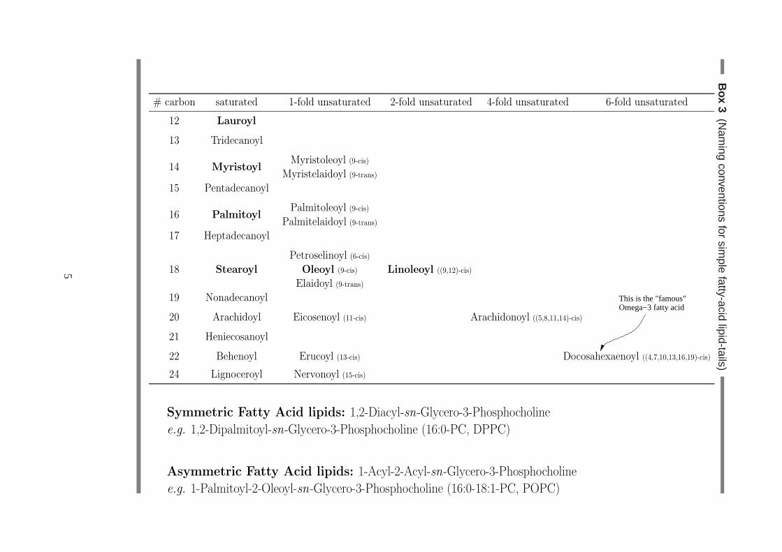
What is the difference between the curvature of a curve and that of a surface? Consider, forinstance, some curved surface, and a curve winding on it. Forthe sake of a picture, think of it asthe path of an all-terrain vehicle in a mountainous environment.9 The path will not be a straightline. Why? There are two fundamentally different reasons for that. First, the terrain is hilly, so thevehicle will go up and down, and may also get deflected sideways10 by the curved underground.This is something the driver cannot do anything about, he or she has to live with the terrain that isgiven. However, the driver could also actively turn the steering wheel, which will give his or herpath a curvature that has nothing to do with the local ground conditions. Specifically, it could evenlead to a curved path on a completely flat terrain. Hence, whenlooking at a curve on a surface,one cannot readily identify the curvature of the curve with the curvature of the surface. First onehas to disentangle these two different contributions. How does that work?The trick is to look at two (unit) vectors: One is the local normal vectorn of the surface, and theother is the principal normalp of the curve,i. e., the direction in which the curve locally curves.The key point is that these vectors need not coincide – see Fig. 3 for the following. Think on theone hand of a vehicle driving along the equator of a sphere. The local normal vector of the spherepoints locally upward11, while the principal normal of the curve points towards the center of thesphere. Hence, both vectors are collinear. Indeed, in this situation the driver drives as straight aspossible, the steering wheel is not turned at all. Now think on the other hand of a driver driving ina circle on a flat ground. The local normal of the underground points upward, while the principalnormal of the driver’s path points horizontally towards thecenter of the circle; the two vectorsnow make an angle of90◦. In this case the curvature of the driver’s path is 100% due tothe factthat the steering wheel is turned and has nothing to do with surface curvature (which in this case

9No trees, though. We want a smooth surface!10You don’t see how a sideways deviation can occur without turning the wheel? Then think for a minute what the

path of the vehicle would look like if it crosses a valley which is deeper to the right than to the left.11Whether it points “upward” or “downward” is a convention we’re free to choose for every (orientable) surface.

12

p p

n

n

R R

b)a)

Figure 3: Disentanglement of the curvature of a curve and that of the underlying surface by theangle between the principal normalp and the surface normaln. Both Figures show a circle ofradiusR and curvature1/R. However, in a) this curvature is entirely due to the surfacethe circlerests on (a car on this path would not have to turn its steeringwheel), while in b) the curvature isentirely due to the curve (the driver would have to turn the steering wheel to the left).

is even zero). Indeed, it may be shown that the localcurvature of the curvemultiplied by thescalar product between the two normal vectors, p · n, is a curvature that no longer depends on anyproperty of the curve,except its direction[14].12 This resulting curvature is called thedirectionalcurvatureor normal curvatureinto the local direction of the curve, and we may write this formallyas

csurface, direction ofγ = ccurveγ p · n = ccurveγ cos ϑ , (16)

whereϑ is the angle betweenp andn. Incidentally, the combinationccurveγ sin ϑ can be identifiedas the counterpart of the directional curvature. It is the amount of curvature which is exclusivelydue to the curve alone,i. e., due to the turning of the steering wheel. It is called thegeodesiccurvature. This completes the disentanglement we have sought for.13

At every point a surface thus has a directional curvature in each direction. Since there are infinitelymany directions, there may also be infinitely many curvatures. But don’t fret, the situation ismuch less unpleasant than it might initially seem. It turns out that there are always two directions,and they are even orthogonal (but not necessarily unique), in which the directional curvatures areextremal. These directions are calledprincipal directions, and the corresponding curvatures arecalledprincipal curvatures. Once we know these directions and the corresponding curvatures, wecan calculateeverydirectional curvature by means of a formula derived first by Euler [14]:

c(α) = c1 cos2 α + c2 sin2 α , (17)

whereα is the angle between the chosen direction and the principal direction belonging to curva-turec1. It thus suffices to know only two curvatures and maybe some directional information.

12Incidentally, this curvature coincides with the local curvature of the cross-cut curve which originates when weintersect our surface with a plane spanned by the local surface normal and the surface direction in question.

13As a side note: Curves on a surface whose geodesic curvature vanishes everywhere are calledgeodesics. These arethe generalization of what straight lines are on a plane. On asphere they are for instance great circles. Fig. 3 alsoillustrates, how a circle of radiusR, which has a simple curvature1/R when viewed as a curve embedded inR

3,can have anything between geodesic curvature 0 – if viewed asa curve on a sphere of radiusR (a great circle) –or geodesic curvature1/R – if lying in a flat plane. Geodesics play a fundamental role inGeneral Relativity, sincethe paths of all particles as well as of light rays are geodesics in spacetime.

13

Let us finally define two more quantities:

extrinsic curvature: K := c1 + c2 , (18a)

Gaussian curvature: KG := c1 c2 . (18b)

Sometimes one also findsH := K/2, the so-calledmean curvature, and in more differentialgeometry flavored texts one findsR := 2KG, the so-calledRicci scalar curvature.

3.2 Monge parametrization

It is all well to talk in geometrical terms about surface curvatures. However, what if we want toactuallycalculatethem? Well, in this case we first have to solve a more fundamental problem,namely: How do we describe the surface to begin with?There are many answers to the question of how to describe a surface embedded in three-dimensionalspace. Some more sophisticated, some less. Some particularly adapted to special symmetries,some not. We will not go into any deeper detail here and ratherpick only one particular surfacedescription, the so-calledMonge parametrization. It is not the most general one, and it is noteven the most convenient one for many applications. But it isfair to say that it is the one whichone encounters most frequently in the literature. It is suitable for surfaces which on average arehorizontal and which don’t have any “overhangs”. In such a case the surface can evidently bedescribed by specifying its heighth above some arbitrarily chosen horizontal reference plane.If r

is the two-dimensional position vector in that plane, thenh(r) is the corresponding height.We now want to calculate the curvatureK within Monge gauge. Box 5 shows a very elementaryway for how this is done in one dimension. The calculation fora surface is a fair bit more involved,and it is advisable to use proper differential geometric techniques for its derivation which we do notwant to introduce here (see Ref. [6] for more details). However, it turns out that the final formulacan be expressed very compactly in a way which resembles the second expression in Eqn. (19). Itis given by

K = ∇ ·(

∇h(r)√

1 + (∇h(r))2

)

|∇h|≪1≈ ∆h(r) , (20)

where∇ and∆ are the nabla- and Laplace-operatoron the base plane, respectively. The approx-imation in the second step is evidently good when the gradient term∇h has a magnitude smallcompared to one, and it is thus referred to as thesmall gradient approximation.It should be remembered, once more, that thesignof K is a matter of convention. In the presentchoice a surface bending “up” has a positive curvature.

4 Helfrich theory

It is time to finally come back to membranes and their curvature elasticity. In this section we wantto study the complete version of curvature elasticity, of which we have already seen a preliminaryversion in the form of Eqn. (14). We then want to look at a few simple consequences that can bederived from this theory.

14

Box 5 (Curvature of a planar curve given in Monge parametrization)Given a function f(x), we want to determinethe local curvature at the point P = (x0, f(x0)).Let’s first find the center of the circle of curva-ture touching at P . It must lie somewhere on thenormal n1(x) through the point P , which has theequation

n1(x) = f(x0) −x − x0

f ′(x0)≡ f0 −

x − x0

f ′0

.

If we deviate a tiny bit dx away from x0, we canconstruct a slightly different normal n2(x). Sincewe are interested in the touching curvature cir-cle, all neighboring normals should to first orderin dx go through the center of the curvature circletouching at P . The equation for such a neighbor-ing normal n2(x) is

c c

x0

y0

0f’(x )

1n (x)

2n (x)

0f’(x )−1 /

(x ,y )R

xdx

f(x)

y

n2(x) = f(x0 + dx) − x − x0 − dx

f ′(x0 + dx)≈ f0 + f ′

0dx − x − x0 − dx

f ′0 + f ′′

0 dx.

The x-position xc of the curvature circle must thus satisfy n1(xc) = n2(xc) up to first order in dx.Solving this equation readily leads to the center coordinates

xc = x0 −f ′0(1 + f ′2

0 )

f ′′0

and yc = n(xc) = f0 +1 + f ′2

0

f ′′0

.

Hence, the radius of curvature ρ of the touching curvature circle satisfies

ρ2 = (xc − x0)2 + (yc − f0)

2 =(1 + f ′2

0 )3

f ′′20

,

and the local curvature K at any point with horizontal coordinate x is thus given by

K =1

ρ=

f ′′(x)

(1 + f ′(x)2)3/2=

(

f ′(x)√

1 + f ′(x)2

)′|f ′|≪1≈ f ′′(x) . (19)

4.1 The Helfrich Hamiltonian

We have seen in Sec. 2.2 that the curvature energy density canbe written as a bending modulustimes the local curvature squared. Since then we have learned a fair bit more about curvature. Inwhich way does this help us to write down a complete energy functional – a Hamiltonian?In 1970 Canham [3] proposed that we should generalize Eqn. (14) in the following way:Ebend =12κ1c

21+

12κ2c

22, where theci are the principal curvatures and theκi the corresponding elastic moduli.

However, if the material isisotropic, κ1 and κ2 should be identical, since bending in the twodifferent directions should not be observable as an energy difference. Canham thus proposed the

15

bending energy density [3]

ebend,Canham =1

2κ(c2

1 + c22) (21a)

=1

2κ(K2 − 2KG) (21b)

Still, we clearly have two independent curvatures, wouldn’t we also expect two moduli?In 1973 Helfrich [12] proposed a slightly different energy density:

ebend,Helfrich =1

2κ(c1 + c2 − c0)

2 + κc1c2 (22a)

=1

2κ(K − c0)

2 + κKG . (22b)

It features two moduli,κ andκ, termed the “bending modulus” and the “saddle splay modulus”,respectively. It also contains a characteristic curvaturec0, called the “spontaneous curvature”.If it is nonzero, this means that the membrane would like to bespontaneously curved into onedirection, which is of course only possible if the membrane is not up-down symmetric,i. e., if ithas two different sides. This, for instance, occurs when thelipid compositions in the two leafletsis different, as it is frequently the case in biology [16, Chap. 1]. However, in the following we willonly look at the simpler cases in whichc0 = 0.We now have two expressions for the energy density. Which oneis right? As it turns out, theanswer is that in most casesboth are right. How can that be – they clearly look different! Theanswer is that there exists a subtle and beautiful theorem from differential geometry – called theGauss-Bonnet-Theorem – which states that the surface integral over the Gaussian curvatureKG canbe written as a boundary term14 and a topological constant [5, 7, 14]. But since the total membraneenergy of course involves a surface integral over (21) or (22), theKG terms in these equations willboth only lead to constants which don’t influence the subsequent physics. And what remains – inthe casec0 = 0 – is in both cases1

2κK2. So modulo boundary terms both Hamiltonians agree – and

indeed only one relevant15 elastic constant appears. However, the Helfrich expression is usuallypreferred over Canham’s equation, because it nicely singles out the Gaussian curvature – which,as we have just seen, has this Gauss-Bonnet specialty.So, let us for completeness write down the total bending energy of a symmetric membrane in theHelfrich picture:

Ebend =

∫

membranedA

{1

2κK2 + κKG

}

. (23)

The integral extends over the entire membrane, anddA is the area elementon the membrane.Box 6 explains that in Monge parametrization it is given bydA = dx dy

√

1 + (∇h)2.In small gradient approximationdA = (1 + 1

2(∇h)2)dx dy. Hence, if we also want to add a term

which penalizesarea increasedue to the curving of the surface, it would enter in small gradientapproximation by a density1

2Σ(∇h)2, whereΣ is the surface tension. Hence, in this approximation

the Helfrich Hamiltonian – including bending and tension, and excluding the Gaussian term – can

14This boundary term involves thegeodesic curvature.15This is really a bit simplified. There are of course instanceswhere boundary and/or topology changes occur, and

thenκ also plays a role. For a nice example, see Ref. [1].

16

Box 6 (Area element in Monge parametrization)Take some point P on a surface with coordinates (x, y, h(x, y)). A point Px a distance dx in x-direction has the coordinates (x + dx, y, h(x + dx, y)) ≈ (x + dx, y, h(x, y) + hx(x, y)dx), wherehx = ∂h/∂x. So the vector

−−→PPx from P to Px is approximately (1, 0, hx)dx. We can do the same

consideration for a point Py a distance dy in y direction. The vectors−−→PPx and

−−→PPy span a little

parallelogram, whose area is equal to the modulus of the cross product between these vectors.Since

10hx

dx ×

01hy

dy =

−hx

−hy

1

dxdy ,

we thus obviously get

dA =∣∣∣−−→PPx ×−−→

PPy

∣∣∣ =

√

1 + h2x + h2

y dxdy =√

1 + (∇h)2 dxdy .

be written as

Ebend =1

2

∫

base planedx dy

{

κ(∆h)2 + Σ(∇h)2}

. (24)

It is this form in which one probably finds the Helfrich Hamiltonian most often. But recall that inthis version it is already a small gradient approximation.

4.2 The shape equation of linear theory

Assume that we have an essentially flat membrane, which is here or there perturbed in such away that it slightly deviates from its flat state, in which it evidently would have the lowest energy– namely zero. The membrane will try to assume a shape in whichthe resulting energy, eventhough not zero, is at least as small as possible. Which shapedoes the membrane therefore have toassume?

4.2.1 Variation of the energy functional

The question we just encountered is a classical problem fromthecalculus of variations. Given a(scalar) expression – here the energyE – which depends on a whole function – here some integralover differentiated terms of the shape functionh – find that function which minimizes the scalarexpression. This is not nearly as complicated as it seems, one only has to proceed patiently.Let’s assume we perform a small variation of the height function, according to

h(x, y) −→ h(x, y) + δh(x, y) . (25)

What is the concomitant change in the bending energy? Using Eqn. (24), and working only in first

17

order of the small quantityδh, we can calculate

δEbend =1

2

∫

dx dy

{

κ(∆h + ∆δh)2 + Σ(∇h + ∇δh)2

}

− 1

2

∫

dx dy

{

κ(∆h)2 + Σ(∇h)2

}

=

∫

dx dy

{

κ∆h ∆δh + Σ∇h · ∇δh

}

=

∫

dx dy

{

κ[

∇ · (∆h∇δh) − (∇∆h) · ∇δh]

+ Σ[

∇ · (∇hδh) − (∆h)δh]}

. (26)

In the last step we have created two divergence terms,∇ · (some vector). We will later turn theminto boundary terms with the help of the divergence theorem.The whole point of this exercise is toget rid of terms which contain derivatives ofδh in the integral. (As we’ll see soon, we don’t mindthese derivatives in the boundary terms). Since there is onemore none-divergence-term containinga derivative ofδh, let’s repeat this trick once more:

δEbend =

∫

dx dy

{

− κ(∇∆h) · ∇δh − Σ(∆h)δh + ∇ ·[

κ∆h∇δh + Σ∇hδh]}

=

∫

dx dy

{

− κ[

∇ ·((∇∆h) · δh

)− (∆∆h) δh

]

− Σ(∆h)δh

+ ∇ ·[

κ∆h∇δh + Σ∇hδh]}

=

∫

dx dy

{[

κ ∆∆h − Σ ∆h]

δh + ∇ ·[(

κ∆h)

∇δh +(

Σ∇h − κ∇∆h)

δh]}

=

∫

dx dy[

κ ∆∆h − Σ ∆h]

δh

+

∮

ds l ·[(

κ∆h)

∇δh +(

Σ∇h − κ∇∆h)

δh]

. (27)

In the last step we finally used the divergence theorem and rewrote the area integral over∇ ·(some vector) as a closed line integral along the curve surrounding the area we originally integratedover. Withl we denote the unit vector which lies in thex-y-plane and locally pointsperpendicularto the curve encircling the (projected) membrane area and isdirectedoutward16.Recall that for a stationary solution we wantδEbend = 0. This means thatboth the area integralas well as the line integral have to vanish. Let’s look at the area integral first. Since the variationδh(x, y) was a completely arbitrary function (well, small and differentiable, but arbitrary other-wise), the above calculation tells us that the term in squarebrackets has to vanish. This gives us adifferential equation– the so-called Euler-Lagrange equation – whichh has to satisfy in the lowestenergy state:

κ ∆∆h − Σ ∆h = 0 . (28a)

This is a fourth order linear partial differential equation. It is called theshape equation. Byintroducing the lengthλ :=

√

κ/Σ, we can also rewrite it as

∆(∆ − λ−2) h = 0 . (28b)

16We assume orientability here, which is not trivial. However, we do not want to potter around with technicalities.

18

“direct” boundary condition “alternative” boundary condition

first condition fixh require(∆ − λ−2)∇⊥h = 0

second condition fix∇⊥h require∆h = 0

Table 1: Possible choices of boundary conditions for the differential equation (28). For each ofthe two rowsonecondition needs to be fulfilled. Recall the definition of the normal derivative atthe boundary,∇⊥ = l · ∇.

Since the operators∆ and∆− λ−2 evidently commute, the differential equation (28) is solved bytheir eigenfunctions to the eigenvalue 0. This is a neat little insight, because it means that we onlyhave to look for solutions oftwo second orderdifferential equations. But finding these functionsis only a part of the problem, often the easier one. What may turn out to be a real pain is gettingtheboundary conditionsright.

4.2.2 Boundary conditions

Speaking of boundary conditions – where do they come from? Well, we still have the boundary in-tegral which has to vanish, too! How can we make sure that thishappens? Looking at the boundaryterm in Eqn. (27) we see that one way is for instance to demand that both the variationδh as wellas the normal component of its gradient,l · ∇δh =: ∇⊥δh, vanishes everywhere on the bound-ary. If we do not permit these two to vary, this basically means that we want them to always havespecific values for all possible surfaces we “test out” in thefunctional variation. In other words,we fixh and∇⊥h at the boundaryand have thus found a permissible set of boundary conditions!However, this recipe is not theonly possibility by which we can ensure that the boundary integralvanishes. For instance, we might alternatively decide not to fix the value of∇⊥h and can still makethe boundary integral vanish if we instead demand that the expression by which it is multiplied,namely∆h, vanishes everywhere on the boundary. Or we might permit theheighth to vary andrather set its prefactor to zero, giving the conditionΣ∇⊥h = κ∇⊥∆h. These possibilities aresummarized in Table 1.If you have never encountered this line of reasoning, you might be a bit shocked here. Regret-tably often the treatment of variational problems (which you may or may not have come acrossbefore) blissfully ignores the boundary terms. One typically finds either the statement “we pushthe boundaries to infinity” (as if it’s always clear that theywould not pick up some contributionthere) or the disarmingly honest phrase “we assume the boundary terms to vanish”. What is missedin this sloppy way is the quite beautiful insight thatthe requirement of vanishing boundary termsgives us the appropriate boundary conditions! Since there are indeed cases where it is not at allclear what the correct conditions would be, this formal route may even be extremely valuable.

4.2.3 A few worked out examples

Before things get too abstract it is recommendable to take a step back and look, what we haveaccomplished and what we can do with it. This section works out a few examples of shape de-termination that illustrate how the shape equation (28) andthe corresponding boundary conditionsfrom Table 1 are used. Not all examples are directly related to fluid membranes. However, now

19

h0

L

f(x)

x

Figure 4: A fluid membrane is laid over a step edge ofheighth0 and attaches a distanceL away from the edge tothe lower-level substrate. What is the shape the membranewill assume?

that we have understood how to handle bending problems, we might just as well have a bit morefun with it.

1. Membrane spread over a step-edge

Assume we want to calculate the shape of a membrane that smoothly covers a step-edge of heighth0 and touches the lower level a distanceL away, as illustrated in Fig. 4. Since the membraneshape changes only inx-direction, we have a one-dimensional problem,i. e., a functionf(x) tofind, and the Laplacian∆ is simply equal to the second derivatived2/dx2. Two independent eigen-functions belonging to the eigenvalue0 are1 andx, and for the eigenvalueλ−2 we convenientlytakecosh(x/λ) andsinh(x/λ). The shape equation (28) becomesf ′′′′(x) − f ′′(x)/λ2 = 0, anddefining the scaled variablesx := x/λ andℓ := L/λ, we can write its general solution as

f(x) = A + Bx + C cosh(x) + D sinh(x) , (29)

where the integration constantsA . . .D are determined by the four obvious boundary conditions

h0 = f(0) = A + C , (30a)

0 = f ′(0) = B + D , (30b)

0 = f(L) = A + Bℓ + C cosh(ℓ) + D sinh(ℓ) , (30c)

and 0 = λ f ′(L) = B + C sinh(ℓ) + D cosh(ℓ) . (30d)

From Eqn. (30a) followsA = h0 − C, and from Eqn. (30b) followsB = −D. Inserting this intothe remaining two equations (30c) and (30d) yields a simple matrix equation forC andD,

(cosh(ℓ) − 1 sinh(ℓ) − ℓ

sinh(ℓ) cosh(ℓ) − 1

) (CD

)

=

(−h0

0

)

, (31)

which can be readily solved by matrix inversion. We thus find the solution of our shape problem. Itcan be expressed in the following way – not fully simplified, but this way it’s a bit more revealing:

f(x)

h0= 1 −

[cosh(ℓ) − 1

][cosh(x) − 1

]− sinh(ℓ)

[sinh(x) − x

]

[cosh(ℓ) − 1

][cosh(ℓ) − 1

]− sinh(ℓ)

[sinh(ℓ) − ℓ

] (32a)

Σ→0= 1 − 3

(x

L

)2

+ 2(x

L

)3

. (32b)

20

gf(x)

xFigure 5: Illustration of the shape of an elasticsheet which is clamped horizontally at one endand hangs under its own weight.

For Σ > 0 there are two characteristic length scales in the problem:λ and L, and the shapelooks qualitatively different depending on which of these two is the bigger one,i. e., depending onwhetherℓ is small or large compared to1, as the interested reader might want to check.What determinesL? In the simplest case the substrate becomes “sticky” a distanceL away fromthe step and pins the membrane there. A more complicated situation arises when the substrate hasa uniform adhesion energyw per area, and the membrane candecideat which distanceL to detach.For smallL much adhesion energy will be gained, but the membrane has to bend a lot. Conversely,if L is chosen very large, bending will be weak, but a lot of adhesion energy is sacrificed. Atsome optimal distance the energy is minimal. It can be shown [15,§12, prob. 6] that this leads toanother boundary condition – this time for themoving boundaryL – that in the present situationreadsf ′′(L) = 1/ρc, whereρc =

√

κ/2w is the contact radius of curvature. Using Eqn. (32b)this results in the transcendental equationℓ coth ℓ

2− 2 = h0ρc/λ

2 for ℓ, whose solution is easilydetermined numerically. ForΣ → 0 (i. e.λ → ∞) it can be solved exactly:L =

√6h0ρc.

2. Paper bending under its own weight

Assume you have a strip of paper which you hold horizontally.Under its own weight it will benddown, as illustrated in Fig. 5. Which shape will the paper take?Since the strip only bends because its weight pulls it down, gravity must somehow be included.How is that done? The easiest way is to again start with the functional. Let’s say the strip has awidth w, a lengthL, and a mass per unit area ofρ. Describe its location by the functionf(x). Thenthe energy of the bent piece of paper is given by

E = w

∫ L

0

dx{1

2κ(f ′′(x)

)2+ ρgf(x)

}

. (33)

Notice that we have cheated slightly: If the projected length of the strip isL, then its actual lengthis generally longer. In other words, the integral shouldn’treally go up toL. However, for smallbending this is an effect of higher order which we will ignorehere.17

We first need to do the variation of this functional. Now, the first term we know how to deal with,and the second term is extremely easy: The variation off(x) is δf(x) and that’s that. Hence, weend up at the shape equationκf ′′′′(x) + ρg = 0, or in a nicer way:

f ′′′′(x) + ℓ−3 = 0 with ℓ3 =κ

ρg, (34)

where we introduced the lengthℓ for convenience. This is a fourth order linear inhomogeneousdifferential equation. The solution of the homogeneous equation f ′′′′(x) = 0 can be written as

17One has to be careful with such approximations, though: For the case of Euler buckling, to be discussed in Example3, this difference between total length and projected length makes all the difference in the world.

21

a + bx + cx2 + dx3, and an obvious particular solution isf(x) = −x4/(24ℓ3). Hence, the generalsolution is

f(x) = a + bx + cx2 + dx3 − 1

24ℓ3x4 . (35)

Two boundary conditions are obvious, namelyf(0) = 0 (from which followsa = 0) andf ′(0) = 0(from which followsb = 0). However, neitherf nor f ′ have any obvious values at the other endof the strip. But peaking at Table 1, we see that since these values are unspecified, we rather haveto demandf ′′(L) = 0 andf ′′′(L) = 0 (recall thatΣ = 0 here).18 The latter condition givesd = L/(6ℓ3), which together with the former leads toc = −L2/(4ℓ3). If we define the scaledvariablesf = f/L, ℓ = ℓ/L, andx = x/L, we see that the final solution can be written as

f(x) = − x4 − 4x3 + 6x2

24ℓ3. (36)

Up to a scaling prefactor the shape of the solution is thus always the same, unlike in the case of themembrane spreading over a step edge in Example 1, where a second length scale existed,λ, andits relation to the lengthL mattered beyond a simple amplitude scaling.The solution (36) in particular shows that the total sag of the strip isf(1) = −(2ℓ)−3, or

|f(L)| =L4

8ℓ3=

ρgL4

8κ. (37)

This relation is quite interesting, since it permits the determination of the bending modulus ofpaper from a fairly simple measurement. Moreover, using therelation between stretching modulusKstretch and bending modulusκ of an isotropic elastic sheet, as worked out earlier, we obtain anestimate of the stretching modulus of paper:

Kstretch(13)=

12κ

h2=

3ρgL4

2|f(L)|h2, (38)

whereh is the thickness of the paper. Let’s think of a typical paper with ρ = 80 g/m2 andh =0.1 mm. If we let a strip ofL = 10 cm hang over the edge of a table, it would droop down bymaybe2 cm. Hence, the stretching modulus is

Kstretch ≈3 × 0.08 kg

m2 × 10 Nkg × (0.1 m)4

2 × 0.02 m× (0.0001 m)2≈ 0.6 × 106 N

m. (39)

3. Euler buckling

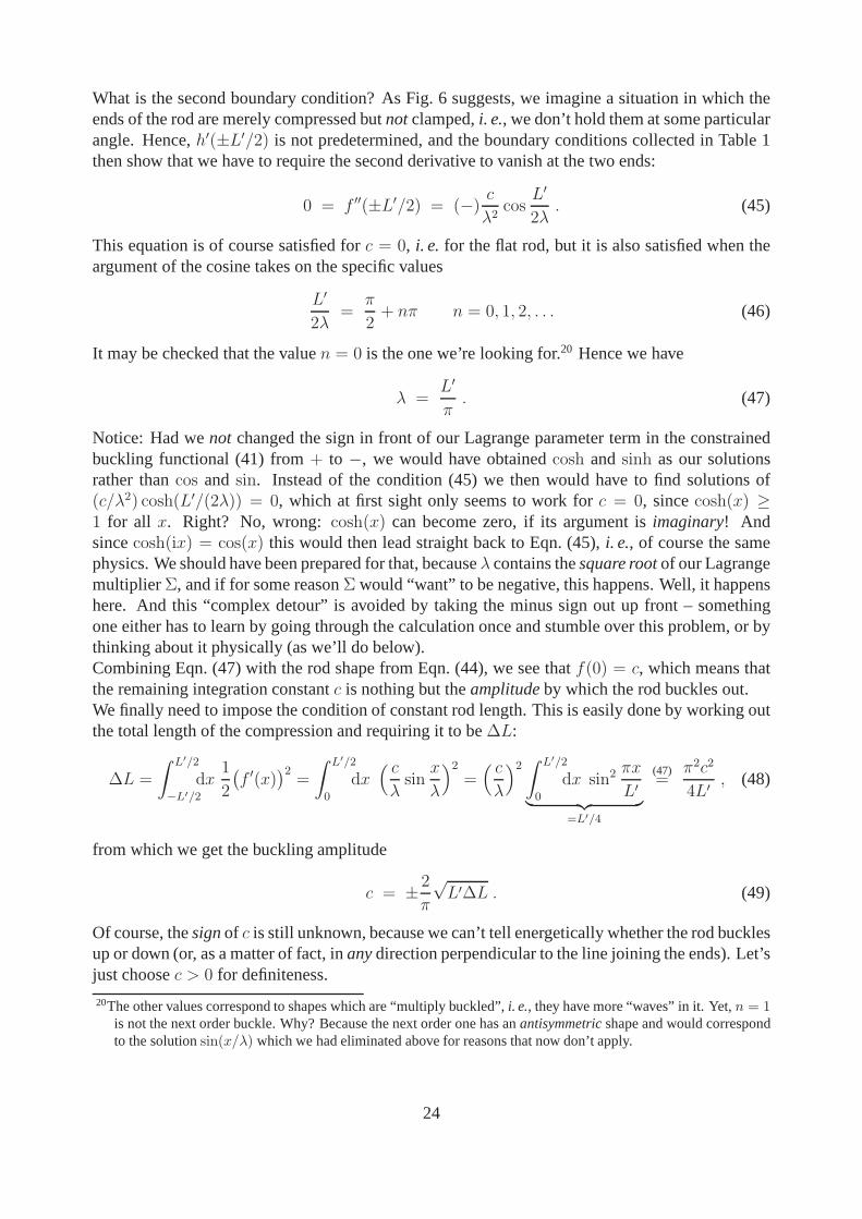
Take a slender elastic rod. Under which compressional forcewill it buckle?Assuming that such a rod is again described by curvature elasticity (just as the strip of paper in theprevious problem was), we will approach the problem in two steps. We first ask ourselves: What isthe bending energy of such a rod of lengthL, if its ends are forced to a separationL′ = L−∆L < L(see Fig. 6). In a second step we will then change to an ensemble where this compression isachieved by an externally applied force.

18Notice that this is a perfect example for the occurrence of the less-than-obvious boundary conditions which never-theless follow easily from the boundary terms of the full variation.

22

−L′/2 +L′/2

f(x)

x

Figure 6: An elastic rod of lengthL iscompressed such that its end-to-end distanceshrinks toL′ = L−∆L < L and consequentlybuckles perpendicular to the direction of com-pression. Notice that the rod ends are fixed, buttheir terminal direction is not (i. e., the ends arenot clamped). The compression in the pictureis δ = ∆L/L = 0.2.

For the energy we may thus use the curvature elastic formula we’ve gotten used to by now:19

E =

∫ L′/2

−L′/2

dx1

2κ(f ′′(x)

)2. (40)

We would like to minimize this functional, subject to the constraint that thetotal lengthof therod has the fixed valueL, or in other words, that the amount of compression,∆L, is given. Asusual, this constraint can be fixed by a Lagrange multiplier,sayΣ, and so we have to minimize theconstrained functional

E ′ =

∫ L′/2

−L′/2

dx

{1

2κ(f ′′(x)

)2 − Σ[1

2

(f ′(x)

)2 − ∆L

L′

]}

. (41)

This expression looks basically like our shape functional from Eqn. (24), with two apparent dif-ferences: First, there is one more constant term in the functional. This of course we need notworry about (who cares about a constant in the energy?). And second, the sign in front of the(f ′(x)

)2-term isnegative. Why is that so? The boring answer is: There is absolutely no physical

significance to this sign! The entire term is multiplied by the Lagrange multiplierΣ, whose value– and thus sign! – needs to be determined later from the constraint. Here we write it with a minussign as this will turn out to be more “convenient”. Had we chosen a positive sign instead, the finalresult would follow identically, albeit with one more twistin thinking, as we will see soon.Minimizing E at constantL means minimizingE ′, i. e. solving the Euler-Lagrange-equation be-longing to the functional (41). With a glance at Eqn. (28) we see that this equation will be

d2

dx2

(d2

dx2+

1

λ2

)

f(x) = 0 , (42)

where we again introducedλ =√

κ/Σ and where the plus-sign stems from the sign difference justmentioned. Once more, the general solution is given by the eigenfunctions of the two commutingsecond order operators belonging to the eigenvalue 0, into which the above fourth order differentialoperator conveniently factorizes, so we can readily write it down:

f(x) = a + bx + c cosx

λ+ d sin

x

λ. (43)

Guessing (correctly) that the (lowest order) buckling willlead to a symmetric situation as depictedin Fig. 6, we see thatb andd have to be zero. Makingh(L′/2) = 0 then leads to

f(x) = c(

cosx

λ− cos

L′

2λ

)

. (44)

19Notice that in this caseκ is a bending energy per unitlengthrather than per unitarea for obtaining a certain radiusof curvature. Therefore,κ has units ofenergy times lengthhere.

23

What is the second boundary condition? As Fig. 6 suggests, weimagine a situation in which theends of the rod are merely compressed butnotclamped,i. e., we don’t hold them at some particularangle. Hence,h′(±L′/2) is not predetermined, and the boundary conditions collected in Table 1then show that we have to require the second derivative to vanish at the two ends:

0 = f ′′(±L′/2) = (−)c

λ2cos

L′

2λ. (45)

This equation is of course satisfied forc = 0, i. e. for the flat rod, but it is also satisfied when theargument of the cosine takes on the specific values

L′

2λ=

π

2+ nπ n = 0, 1, 2, . . . (46)

It may be checked that the valuen = 0 is the one we’re looking for.20 Hence we have

λ =L′

π. (47)

Notice: Had wenot changed the sign in front of our Lagrange parameter term in the constrainedbuckling functional (41) from+ to −, we would have obtainedcosh and sinh as our solutionsrather thancos and sin. Instead of the condition (45) we then would have to find solutions of(c/λ2) cosh(L′/(2λ)) = 0, which at first sight only seems to work forc = 0, sincecosh(x) ≥1 for all x. Right? No, wrong:cosh(x) can become zero, if its argument isimaginary! Andsincecosh(ix) = cos(x) this would then lead straight back to Eqn. (45),i. e., of course the samephysics. We should have been prepared for that, becauseλ contains thesquare rootof our Lagrangemultiplier Σ, and if for some reasonΣ would “want” to be negative, this happens. Well, it happenshere. And this “complex detour” is avoided by taking the minus sign out up front – somethingone either has to learn by going through the calculation onceand stumble over this problem, or bythinking about it physically (as we’ll do below).Combining Eqn. (47) with the rod shape from Eqn. (44), we see thatf(0) = c, which means thatthe remaining integration constantc is nothing but theamplitudeby which the rod buckles out.We finally need to impose the condition of constant rod length. This is easily done by working outthe total length of the compression and requiring it to be∆L:

∆L =

∫ L′/2

−L′/2

dx1

2

(f ′(x)

)2=

∫ L′/2

0

dx( c

λsin

x

λ

)2

=( c

λ

)2∫ L′/2

0

dx sin2 πx

L′

︸ ︷︷ ︸

=L′/4

(47)=

π2c2

4L′, (48)

from which we get the buckling amplitude

c = ±2

π

√L′∆L . (49)

Of course, thesignof c is still unknown, because we can’t tell energetically whether the rod bucklesup or down (or, as a matter of fact, inanydirection perpendicular to the line joining the ends). Let’sjust choosec > 0 for definiteness.

20The other values correspond to shapes which are “multiply buckled”, i. e., they have more “waves” in it. Yet,n = 1is not the next order buckle. Why? Because the next order one has anantisymmetricshape and would correspondto the solutionsin(x/λ) which we had eliminated above for reasons that now don’t apply.

24

1

4(F − 1)

F = F/Fbuckle = FL2/κπ2

δ=

∆L

/L

109876543210

0.5

0.4

0.3

0.2

0.1

0

Figure 7: Stress-strain relation (53) for an elastic rod under compression.

Now that we know the shape, we can calculate the energy of the buckled rod:

E =

∫ L′/2

−L′/2

dx1

2κ(f ′′(x)

)2= κ

∫ L′/2

0

dx

(d

λ2cos

x

λ

)2

=κπ2∆L

(L − ∆L)2=

κπ2

L

δ

(1 − δ)2, (50)

where we introduced the scaled compressional strainδ = ∆L/L. This energy initially growslinearly with compression, but later it increases more strongly.It is now time to think about the compressionforce. We have so far looked at the situation in an“ensemble” of constantcompression(i. e., strain) and would now like to change to an ensemble ofconstantforce(i. e., stress). As usual, this is accomplished by a Legendre transformation:

G(F ) = min∆L

{

E(∆L) − F ∆L}

=κπ2

Lmin

δ

{ δ

(1 − δ)2− F δ

}

, (51)

where we introduced the scaled force

F =FL2

κπ2. (52)

Doing the minimization, we see that we have to solve the equation21

(1 − δ)2 + 2δ(1 − δ)

(1 − δ)4− F = 0 or F =

1 + δ

(1 − δ)3= 1 + 4δ + 9δ2 + 16δ3 + · · · (53)

This stress-strain relation is illustrated in Fig. 7. A positive compressionδ > 0 requires a (scaled)compression forceF ≥ 1. The initial stress-strain relation isnot simply linear. One has to over-come a certain minimal force – the buckling force – before therod will deflect:

F ≥ Fbuckle =κπ2

L2. (54)

21Of course, we might have guessed Eqn. (53) right away – it is nothing but a statement of the “obvious” fact thatF = ∂E/∂∆x. In some sense, the Legendre trafo shows, why this “obvious”fact indeed holds.

25

Eqn. (50) and its initial linear energy-compression relation shows rather vividly how strongly non-harmonic Euler buckling is. For a usual harmonic energy,i. e. E ∝ (∆x)2, the force would(linearly) go to zero as the compression goes to zero. Not so here: In the limit of vanishingcompression afinite force remains, the buckling force, which – conversely – firstneeds to beovercome in order to compress the rod. Notice also that afterFbuckle is exceeded the resultingdeflection is quite finite. The rod does of coursenot catastrophically fail once the buckling limit isexceeded.This scenario looks a bit like a second order “phase transition”, even though a somewhat unusualone: If F is the “driving variable” andδ the “order parameter”, than∂δ/∂F doesnot divergeat the “critical” point but rather assumes the finite value1/4, while it has the value0 below thetransition.22

4.2.4 Nonlinear shape equation

Recall that the small gradient Hamiltonian (24) only was an approximation to the full expression(23). The full Hamiltonian can also be varied, giving rise toa shape equation. This variation is a bitmore tedious to perform, but it can be done exactly.23 However, the equation one now ends up withis a fourth ordernonlinearpartial differential equation [11, 17]. It is outrageouslydifficult to solve,and there existvery few exact solutions. However, many interesting problems involve membraneswhich are not essentially flat, such as for instance closed vesicles, and a lot ofnumericalresearchhas thus been devoted (in the early 1990s) to understand specific solutions of the nonlinear shapeequation. The reader will find a very good introduction to this (and much more in fact) in thereview by Seifert [21].

4.3 Membrane fluctuations

The fact that the small-gradient version of the Helfrich Hamiltonian, Eqn. (24), is quadratic, im-plies that the shape equation (28) is linear. But it also means that we can rather easily treat addi-tional thermal fluctuations, because the partition function of quadratic Hamiltonianscan be easilyworked out. In fact, we don’t even have to do this, the equipartition theorem will suffice for whatwe want to look at now.We start by Fourier-expanding the membrane shapeh(r). For this we assume that the membranespans a quadratic frame of sizeL × L, and for convenience we assume periodic boundary condi-tions. The shape can then be expanded in a Fourier series according to

h(r) =∑

q

hq eiq·r , q =2π

L

(nx

ny

)

, nx, ny ∈ Z . (55)

Since the membrane surfaceh(r) is a real function, the complex Fourier modes must satisfy the

22If you want, the critical exponentβ takes on the unusual valueβ = 0.23A particularly clever method, which relies on fixing the tedious geometrical constraints by Lagrange multiplier

functions, has recently been proposed by Guven [11].

26

conditionh−q = h∗q. Using this, we find immediately

∇h =∑

q

hq iq eiq·r , (56a)

(∇h)2

=∑

q,q′

hqhq′ (−q · q′) ei(q+q′)·r , (56b)

∇2h =

∑

q

hq (−q2) eiq·r , (56c)

(∇

2h)2

=∑

q,q′

hqhq′ (q2q′2) ei(q+q′)·r . (56d)

If we now make use of the Fourier representation of the Kronecker-δ

∫

L×L

d2r e−iq·r = L2 eiqL/2 sin qL2

qL2

= L2 δq,0 , (57)

we find upon inserting Eqns. (56) back into the small gradientenergy (24)

Ebend =

∫

L×L

d2r∑

q,q′

hqhq′ ei(q+q′)·r

{1

2κ(q2q′2) +

1

2Σ(−q · q′)

}

=∑

q,q′

hqhq′ L2 δq+q′,0

{1

2κ(q2q′2) +

1

2Σ(−q · q′)

}

= L2∑

q

hqh−q

{1

2κq4 +

1

2Σq2

}

= L2∑

q

|hq|2{

1

2κq4 +

1

2Σq2

}

. (58)

This tells us several things:

1. Whether a particular undulation mode costs predominantly bending energy or tension energyis a question of the wave vector. For wave vectors smaller than qcrossover :=

√

Σ/κ, i. e. onlarge length scales, tension is the dominant energy contributing to Eqn. (58). Conversely, forwave vectors bigger thanqcrossover, i. e.on small length scales, bending dominates.

2. In Fourier space the membrane energy is diagonal,i. e., the different wave vectors decouple:

〈hqhq′〉 = 〈|hq|2〉 δq,−q′ . (59)

3. These modes areharmonic, i. e., we can simply use the equipartition theorem to get

L2 〈|hq|2〉{

1

2κq4 +

1

2Σq2

}

=1

2kBT . (60)

Equation (60) immediately gives us the important result

〈|hq|2〉 =kBT

L2[κq4 + Σq2

] . (61)

27

Eqn. (61) is thefluctuation spectrumor static structure factorof a membrane. It tells us the mean-square-amplitude of membrane modes. Since they are thermally excited, they are also proportionalto temperature: More fluctuations give bigger amplitudes. Importantly, the fluctuation spectrumdepends on the elastic constantκ and on the applied tensionΣ. Measuring the fluctuation spectrumand fitting to Eqn. (61) is thus a viable method to extract the bending modulus in an experiment.The method is calledflicker spectroscopy[2, 9, 20].What kind of average undulation amplitude do we have to expect for the entire membrane, andnot just for a single mode? Evidently, the full membrane amplitude is the sum over all individualmodes, and we can easily calculate

〈h2〉 =∑

q

〈|hq|2〉 =∑

q

kBT

L2(κq4 + Σq2)≈(

L

2π

)2 ∫ qmax

qmin

dq 2πqkBT

L2(κq4 + Σq2)

=kBT

4πΣln

q2max(q

2minκ + Σ)

q2min(q

2maxκ + Σ)

Σ→0−→ kBT

4πκ

q2max − q2

min

(qmaxqmin)2≈ kBT

16π3κL2 , (62)

where we in the first line replaced the sum by an integral, in which we introduced a large wave-length cutoffqmin = 2π/L and a small wavelength cutoffqmax = 2π/a, wherea is comparable tobilayer thickness. In the last step we neglectedq2

min againstq2max in the numerator.

The final approximate relation gives rise to a nice rule of thumb: Since a very typical value for thebending stiffness isκ = 20 kBT , inserting it we readily find

∆h ≡ 〈h2〉1/2 ≃ L

100(Σ = 0, κ ≈ 20 kBT ) , (63)

i. e., the root mean square amplitude of the membrane fluctuationsunder vanishing tension aretypically about 1% of the lateral extension of the membrane.Notice the scale invariance inherentin such a statement. Of course, if the membrane is under tension, this value is reduced.

References[1] J.-M. Allain, C. Storm, A. Roux, M. Ben Amar, and J.-F. Joanny,Fission of a multiphase membrane tube, Phys.

Rev. Lett.93, 158104 (2004).

[2] F. Brochard and J.F. Lennon,Frequency spectrum of flicker phenomenon in erythrocytes, J. Phys. (Paris)36,1035 (1975).

[3] P.B. Canham,The minimum energy of bending as a possible explanation of the biconcave shape of the humanred blood cell, J. Theoret. Biol.26, 61 (1970).

[4] I.R. Cooke and M. Deserno,Coupling between Lipid Shape and Membrane Curvature, Biophys. J.91, 487(2006).

[5] F. David, in: Statistical Mechanics of Membranes and Surfaces, ed. by D. Nelson, T. Piran, and S. Weinberg,2nd ed., (World Scientific, Singapore, 2004).

[6] M. Deserno,Notes on Differential Geometry; a pdf file can be downloaded here:http://www.mpip-mainz.mpg.de/∼deserno/scripts/diff geom/diff geom.pdf

[7] M. Do Carmo,Differential Geometry of Curves and Surfaces, Prentice Hall, Englewood Cliffs (1976).

[8] E. Evans and D. Needham,Physical Properties of Surfactant Bilayer Membranes: Thermal Transitions, Elastic-ity, Rigidity, Cohesion, and Colloidal Interactions, J. Phys. Chem,91, 4219 (1987).

28

[9] J.F. Faucon, M.D. Mitov, P. Meleard, I. Bivas, and P. Bothorel, Bending elasticity and thermal fluctuations oflipid-membranes – Theoretical and experimental requirementsJ. Phys. (Paris)50, 2389 (1989).

[10] G. Graziano,Cavity Thermodynamics and Hydrophobicity, J. Phys. Soc. Japan69, 1566 (2000).

[11] J. Guven,Membrane geometry with auxiliary variables and quadratic constraints, J. Phys. A: Math. Gen.37,L313 (2004).

[12] W. Helfrich, Elastic properties of lipid bilayers – theory and possible experiments, Z. Naturforsch. C28, 693(1973).

[13] J.N. Israelachvili, D.J. Mitchell, and B.W. Ninham,Theory of self-assembly of hydrocarbon amphiphiles intomicelles and bilayers, J. Chem. Soc., Faraday Trans. 272, 1525 (1976).

[14] E. Kreyszig,Differential Geometry, Dover, New York (1991).

[15] L.D. Landau and E.M. Lifshitz,Theory of Elasticity, Butterworth-Heinemann, Oxford (1999).

[16] R. Lipowsky and E. Sackmann (eds.),Structure and Dynamics of Membranes, Handbook of Biological Physics,Vol. 1A (Elsevier, New York/North-Holland, Amsterdam, 1995).

[17] Z.-C. Ou-Yang and W. Helfrich,Bending energy of vesicle membranes – General expression for the 1st, 2nd and3rd variation of the shape energy and applications to spheres and cylinders, Phys. Rev. A39, 5280 (1989).

[18] T.A. Ozal and N.F.A. van der Vegt,Confusing Cause and Effect: Energy-Entropy Compensation in the Pref-erential Solvation of a Nonpolar Solute in Dimethyl Sulfoxide/Water Mixtures, J. Phys. Chem. B110, 12104(2006).

[19] W. Rawicz, K.C. Olbrich, T. McIntosh, D. Needham, and E.Evans,Effect of chain length and unsaturation onelasticity of lipid bilayers, Biophys. J.79, 328 (2000).

[20] M.D. Schneider, J.T. Jenkins, and W.W. Webb,Thermal fluctuations of large quasi-spherical bimolecularphos-pholipid vesiclesJ. Phys. (Paris)45, 1457 (1984).

[21] U. Seifert,Configurations of fluid membranes and vesicles, Adv. Phys.46, 13 (1997).

[22] N.T. Southall, K.A. Dill, and A.D.J. Haymet,A View of the Hydrophobic Effect, J. Phys. Chem. B106, 521(2002).

[23] N.F.A. van der Vegt, D. Trzesniak, B. Kasumaj, and W.F. van Gunsteren,Energy-entropy compensation in thetransfer of nonpolar solutes from water to cosolvent/watermixtures, Chem. Phys. Chem.5 144 (2004).

29