Embed Size (px)
Citation preview
FLUID FLOW AT SMALL
REYNOLDS NUMBER:
Numerical Applications
Tayfour El-Bashir
Department of Mathematics and Statistics, College of Science
Sultan Qaboos University P.O. Box 36, Al-Khod 123
Sultanate of Oman
HIKARI LT D
HIKARI LTD
Hikari Ltd is a publisher of international mathematical journals and books.
www.m-hikari.com
Tayfour El-Bashir, FLUID FLOW AT SMALL REYNOLDS NUMBER: Nu-
merical Applications, First published 2006.
No part of this publication may be reproduced, stored in a retrieval system,
or transmitted, in any form or by any means, without the prior permisson of
the publisher Hikari Ltd.
Typeset using LATEX.
Mathematics Subject Classification: 65N38, 74S20, 68Q85
Keywords: Slow flow, cylinder, rotlet, boundary element method
Published by Hikari Ltd
PREFACE
This book is concerned with the numerical solution of the Navier-Stokes equations
for some steady, two-dimensional, incompressible viscous fluid flow problems at small
and moderate values of the Reynolds number.
The first problem relates to a two-dimensional, incompressible flow both with and
without a line rotlet at various small values of the Reynolds number. A circular
cylinder of radius a is rotated with a constant angular velocity ω0 in the presence of
a uniform stream of magnitude U. Two techniques are introduced, one in order to
avoid the difficulties in satisfying the boundary conditions at large distances from the
cylinder, the other to achieve convergence of the solution at zero Reynolds number.
Transformations are applied to both the coordinate system and the stream function.
The second problem considers the solution of the biharmonic equation for the
slow viscous flow generated by a line rotlet in the presence of a circular cylinder.
On identifying the coefficients of some of the terms in the asymptotic expansion of
the stream function, in terms of the force components and the torque on the body,
and using an integral constraint, the Boundary Element Method provides a closed
system of equations. Excellent agreement is obtained between the numerical results
and the analytical expressions and some new results relating to forces and torques on
the cylinder are presented.
In the third problem the solution of the biharmonic equation, which represents the
Stokes flow created by two rotating circular cylinder in which the force system acting
on the two cylinders is in a state of overall equilibrium is examined. In this situation
the total force and the total torque are both assumed to be zero and the Boundary
Element Method, together with the relationships between the forces and the torque on
the combined system and the coefficients in the asymptotic expansion for the stream
function, is applied.
The final problem relates to a line rotlet outside an elliptical cylinder and the
solution shows that it is possible to generate a flow at infinity which corresponds to
that of rigid body rotation. This contrary to the situation for a line rotlet outside
a circular cylinder, where the fluid flow at infinity corresponds to that of a uniform
stream which is the direction perpendicular to the line joining the rotlet to the center
of the cylinder.
Tayfour El-Bashir
Sultan Qaboos University
August, 2006
Contents
1 INTRODUCTION 1
1.1 The Navier-Stokes Equations . . . . . . . . . . . . . . . . . . . . 1
1.2 Stokes Paradox . . . . . . . . . . . . . . . . . . . . . . . . . . . . 2
1.3 Work by Jeffery (1922) . . . . . . . . . . . . . . . . . . . . . . . . 5
1.4 Work by Dorrepaal, O’Nei11 and Ranger (1984) . . . . . . . . . . 6
1.5 Existence of Possible Paradoxical Flows . . . . . . . . . . . . . . 6
1.6 The Outline . . . . . . . . . . . . . . . . . . . . . . . . . . . . . . 8
2 ROTATING CIRCULAR CYLINDER AND A ROTLET 17
2.1 Introduction . . . . . . . . . . . . . . . . . . . . . . . . . . . . . . 17
2.2 Basic Equations and the Boundary Conditions . . . . . . . . . . 20
2.3 The Solution Technique . . . . . . . . . . . . . . . . . . . . . . . 26
2.4 Results . . . . . . . . . . . . . . . . . . . . . . . . . . . . . . . . . 33
2.5 Conclusion . . . . . . . . . . . . . . . . . . . . . . . . . . . . . . 36
3 ANALYTICAL SOLUTION 47
3.1 Solution Using Fourier Series . . . . . . . . . . . . . . . . . . . . 47
3.2 Forces and Moment on the Cylinder . . . . . . . . . . . . . . . . 51
3.3 Method of Obtaining the Forces . . . . . . . . . . . . . . . . . . . 54
3.4 Relations between the Forces . . . . . . . . . . . . . . . . . . . . 58
3.5 Flows at Infinity . . . . . . . . . . . . . . . . . . . . . . . . . . . 61
3.6 Conclusions . . . . . . . . . . . . . . . . . . . . . . . . . . . . . . 65
4 FLOW GENERATED BY A ROTLET 67
4.1 Introduction . . . . . . . . . . . . . . . . . . . . . . . . . . . . . . 67
4.2 The Boundary Element Method (BEM) . . . . . . . . . . . . . . 72
i
ii CONTENTS
4.3 The Numerical Solution . . . . . . . . . . . . . . . . . . . . . . . 82
4.4 Numerical Results . . . . . . . . . . . . . . . . . . . . . . . . . . 87
4.5 Conclusions . . . . . . . . . . . . . . . . . . . . . . . . . . . . . . 100
5 THE ROTATION OF TWO CIRCULAR CYLINDERS 103
5.1 Introduction . . . . . . . . . . . . . . . . . . . . . . . . . . . . . . 103
5.2 Co-ordinate System . . . . . . . . . . . . . . . . . . . . . . . . . 104
5.3 Stream Function Expansion . . . . . . . . . . . . . . . . . . . . . 108
5.4 Boundary Bonditions . . . . . . . . . . . . . . . . . . . . . . . . . 112
5.5 Linear Equation of the Boundary Conditions . . . . . . . . . . . 114
5.6 Asymptotic Form of the Stream Function . . . . . . . . . . . . . 117
5.7 Validation of the Expansions for hΨ . . . . . . . . . . . . . . . . 120
5.8 Forces and Torques on the Cylinders . . . . . . . . . . . . . . . . 124
5.9 Alternative Expressions for the Forces . . . . . . . . . . . . . . . 130
5.10 Additional Conditions . . . . . . . . . . . . . . . . . . . . . . . . 135
5.11 Boundary Element Method . . . . . . . . . . . . . . . . . . . . . 136
5.12 Results . . . . . . . . . . . . . . . . . . . . . . . . . . . . . . . . . 140
5.13 Conclusions . . . . . . . . . . . . . . . . . . . . . . . . . . . . . . 143
6 ELLIPTICAL CYLINDER AND A ROTLET 151
6.1 Introduction . . . . . . . . . . . . . . . . . . . . . . . . . . . . . . 151
6.2 Forces and Moment on the Ellipse . . . . . . . . . . . . . . . . . 156
6.3 The Governing Equations . . . . . . . . . . . . . . . . . . . . . . 157
6.4 Numerical Solution . . . . . . . . . . . . . . . . . . . . . . . . . . 159
6.5 Numerical Results . . . . . . . . . . . . . . . . . . . . . . . . . . 162
6.6 Conclusions . . . . . . . . . . . . . . . . . . . . . . . . . . . . . . 163
7 CONCLUSIONS 167

Chapter 1
INTRODUCTION
1.1 The Navier-Stokes Equations
One of the simplest steady, two-dimensional fluid flow problems is that of a infi-
nite, stationary, viscous fluid, which is disturbed by a circular cylinder of radius
a moving with a uniform velocity U through it. When the fluid is incompressible
and Newtonian then the governing equations are the continuity equation and
the Navier-Stokes equations, which in dimensionless form, are expressible as
∇∗ . u∗ = 0, (1.1.1)
Du∗
Dt∗=∂u∗
∂t∗+ (u∗.∇∗)u∗ = −∇∗p∗ +
1Re
∇∗2u, (1.1.2)
where (*) denotes the dimensionless form of the physical quantity, t∗ the time, u∗
the fluid velocity vector, p∗ the pressure and Re = aU/ν, with ν the coefficient
of kinematic viscosity, is the Reynolds number. For simplicity the (*)’ s will be
omitted throughout the remainder of this Chapter. When one is concerned with
situations where the fluid is extremely viscous, namely ν large, or the motion of
the body is very slow, so U << 1, then the Reynolds number is very small and
the inertia terms on the left hand side of equation ( 1.1.2 ) can be neglected.
Although a similar conclusion applies for small values of a one must ensure that
this value is not reduced to a level where the continuum model is no longer
applicable.
1
2 CHAPTER 1. INTRODUCTION
When the equations of motion are simplified by the omission of the inertia
terms, i. e. Re << 1, and the motion is two-dimensional then the introduction
of the stream function, so that the continuity equation (1.1.1) is identically
satisfied, by
u =∂ψ
∂yand v = −∂ψ
∂x, (1.1.3)
together with the removal of the pressure by taking the curl of equation (1.1.2),
results in the biharmonic equation
∇4ψ = O. (1.1.4)
It is the solution of this equation that the majority of this book is related
to. When the initial problem of a circular cylinder moving through a fluid is
considered and the Reynolds number parameter Re is assumed small then no
solution of equation (1.1.4) is possible. This phenomenon is usually referred to
as the ”Stokes Paradox” .
1.2 Stokes Paradox
The cause of the Stokes paradox in a two-dimensional flow is that no solution of
the simplified equations can be found for which the fluid velocity satisfies both
the boundary conditions on the body and at infinity, since the solution, which
satisfies all the boundary conditions on the obstacle is unbounded at infinity.
However, the fluid velocity is found to be logarithmically infinite, see Stokes
(1851), thus tends to infinity as the logarithm of the distance from the cylinder,
i.e. it increases slowly with this distance, and so it should give a fairly good
approximation to the fluid motion at small and moderate distances from the
cylinder. In mathematical terms the solution of the Stokes equation, which for
the non-dimensional stream function, ψ, is expressible as
ψ = A sin(θ)[(r
a) ln(
r
a) − 1
2(r
a) +
12(a
r)], (1.2.1)
though valid near the cylinder, does not form a uniformly valid approximation
to the Navier-Stokes equations far from the cylinder.
Briefly, the difficulty arises since any body moving with a constant speed
through a viscous fluid experiences some resistance, and, see Tomotika and
Imai (1938), by considering the momentum flux across a large surface, which
1.2. STOKES PARADOX 3
surrounds the body one can show that the magnitude of the disturbance to
the uniform fluid velocity cannot fall to zero more rapidly than the inverse
square of the distance from the body. This results in a singularity at infinity in
the perturbation solution for non-zero Reynolds number, where the convection
terms at large distances from the body are of the same order of magnitude as
the viscous forces. Hence, the Stokes’s solution fails to provide a uniform valid
approximation to the fluid flow. Only if the disturbance decays exponentially
is it possible for the convection terms to continue to be neglected in the outer
flow region.
It should be noted that for the fluid flow past an sphere the Stokes equation
provides a uniform approximation to the total velocity distribution. This, at
first, appears ’contrary to the situation for a cylinder where, as discussed above,
the solution is unbounded as r becomes infinitely large. This uniformly valid
approximation to the fluid velocity enables properties of the flow, such as the
lift, drag and moment on the sphere, to be determined by the uniformly valid
approximations. The Stokes solution does not break down until the distance
from the body is such that the velocity approaches that of the uniform stream.
Here, the flaw in the solution arises because of the fluid velocity derivatives at
large distances being in error and it is these derivatives in the neglected inertia
terms that are required to obtain the second approximation to the fluid flow.
It is necessary to establish a uniformly valid approximation to the neglected
inertia terms in the Navier-Stokes equation so one can determine the second
approximation to the solution even in the region close to the body. This re-
quires the introduction of an expansion procedure, similar to that described by
Whitehead (1889), in powers of the Reynolds number Re, where the neglected
inertia terms are reintroduced into the equations of motion. Although produc-
ing the correct differential equation for the flow in the region not far from the
body this approach fails to produce a solution, which satisfies the condition at
infinity, even in the case when the body corresponds to a sphere.
Unlike the Stokes solution of steady uniform fluid flow past a sphere there is
no uniform approximation for the case of flow past a two-dimensional cylinder
since the solution is unbounded. In particular it is found from equation 1.2.1
that terms like rln(r)sin(θ) give rise to a non-uniformly valid expression, which
initially appears to make the solution completely unsatisfactory. It is seen that
the neglected inertia terms should be included when Re(rln(r)) is 0(1) and for
4 CHAPTER 1. INTRODUCTION
values of r of this magnitude the classical Stokes solution will be invalid. This
suggests that close to the cylinder the Stokes approximation is a reasonable
representation to the fluid flow, but fails to provide the uniform approximation
to the total velocity distribution.
However, it is possible to rewrite the approximation in such a manner such
that the severity of the non-uniformity appears to be somewhat decreased and
leads one to obtain a uniform stream in that region where the Stokes equation
ceases to be valid and this suggests that the uniform stream condition has been
attained prior to the break down of the approximation. This idea was the basis
of the work by Oseen (1910), where for both the sphere and the cylinder a
uniform approximation to the disturbance of the stream is possible by taking
the inertia terms into account when they are comparable in magnitude to the
viscous terms, namely where the flow is nearly a uniform stream, and neglecting
them close to the body. Oseen (1910) proposed that the inertia terms should be
retained in the far field, where the fluid velocity is approximately equal to U,
since in that region the assumptions underlying the Stokes equation are not valid
at sufficiently large distances from the cylinder no matter how small Re may be.
These inertia terms are of 0(Re) near to the cylinder, where it is permissible to
neglect them altogether, and so one finds that in three-dimensional fluid flow
past an obstacle both the Stokes and Oseen equations yield the same terms,
which are of 0(1), and differ only in the terms of O(Re). However, it was not
until Kaplun and Lagerstrom (1957) and Proudman and Pearson (1957 ) that
the whole process was placed on a rigorous mathematical foundation using the
ideas of matched asymptotic expansions and the technique extended to higher
order approximations for both the two and three-dimensional cases.
As the perturbation theory arising for small non-zero Reynolds numbers is
singular, both the above sets of authors developed a technique for overcoming
this difficulty when expanding in terms of the small Reynolds number param-
eter. Essentially this considers separate local expansions for the regions close
to, and far from, the body, usually referred to as the (inner) Stokes and (outer)
Oseen expansions, respectively. The two sets of differential equations result-
ing from substituting the above expansions into the Navier-Stokes equations
have only one set of physical boundary conditions applicable to each expansion,
namely no slip at the body for the Stokes expansion and the uniform stream
condition for the Oseen expansion. In order to establish a unique solution it is

1.3. WORK BY JEFFERY (1922) 5
necessary to introduce a matching procedure by which the outer solution pro-
vides an outer boundary condition for the inner solution and the inner solution
provides an inner boundary condition on the outer solution. This technique
of matched asymptotic expansions allows for the determination of the alterna-
tively successive terms in the two expansions, as well as the form of the local
expansions for the two regions. Consequently, the solution of the biharmonic
equation for two-dimensional, slow streaming flows in an unbounded fluid may
be interpreted as an inner solution of the Navier-Stokes equations. This solu-
tion will be valid within some finite distance from the body, but requires an
outer solution in order to satisfy the uniform stream condition at infinity, so
explaining how the Stokes Paradox can be overcome.
1.3 Work by Jeffery (1922)
An additional paradox caused by local effects was that discovered by Jeffery
(1922) when two cylinders of equal radii in an unbounded fluid are rotating
with equal speeds, but in opposite senses about parallel axes. Jeffery (1922)
established the presence of a uniform stream at infinity in the direction perpen-
dicular to the line joining the centers of the two cylinders. Al though his result
was known to be in error due to it being impossible to establish within any
finite time no explanation was presented, yet the author must have been aware
of the earlier work by Oseen (1910). It was probably this paradoxical situation,
which caused Jeffery to restrict his solution to that one particular case, even
though he had formulated the problem for two cylinders with different radii
and different angular speeds. This paradox was extended to the general case
by Smith (1991). He found that the above situation uniform flow was present
only when the combined angular momentum of the two cylinders was zero, in all
other cases, instead of the far field corresponding to a uniform stream, a rigid
body rotation occurred.
One striking feature of Jeffery’s and Smith’s solutions was that they re-
stricted their stream function expansion to that corresponding to a finite number
of terms in the Fourier Series describing the solution, which although satisfying
the boundary conditions failed to produce any other physical situation except
that in which the combined system of the two cylinders was in a state of overall
equilibrium, namely zero total force and zero total moment. As Smith (1991)
6 CHAPTER 1. INTRODUCTION
was aware that he was constructing only an inner solution he was able to match,
unfortunately erroneously, with a complete solution of the Navier-Stokes equa-
tions for the outer flow field.
However, it should be stressed that in Watson (1995) the solutions to this
problem and that of a rotlet outside a circular cylinder have been fully developed
using an inner and outer matching technique. The results in the far field of
the outer solution always correspond to a Jet behavior along one of the axes.
Whilst by allowing the complete Fourier Series to represent his solution, Watson
established that the inner condition on the outer solution always represented a
force, so removing the above restriction concerning the equilibrium conditions
on the combined system.
1.4 Work by Dorrepaal, O’Nei11 and Ranger
(1984)
Another example of a paradoxical situation arising from a local affect was pre-
sented by Dorrepaal, O’Nei11 and Ranger (1983) when a rotlet, or stokeslet, is
placed in front of a circular cylinder. However, these authors established that
both Jeffrey’s and their problem are well-posed Stokes flow problems provided
there is a uniform stream at infinity having an appropriate direction and mag-
nitude. Whereas the parameters involved in Jeffery’s case are the radii and the
angular velocities of the cylinders and the distance separating the two cylinders.
In the case of the rotlet it is the position and strength of the rotlet as well as
the radius of the cylinder. Avudainayagam and Jothiram (1987) extended this
work to show that with a particular singularity present in the flow field out-
side a circular cylinder then for a suitably chosen rotational flow at infinity, in
addition to a uniform stream, the problem is also well-posed.
1.5 Existence of Possible Paradoxical Flows
A rotating cylinder produces a somewhat specialized flow in the case of three-
dimensional, slow viscous flow since there is no motion in the direction parallel
to the axis of rotation. This restriction of the flow to planes perpendicular to
the axis allows a stream function to be introduced, which in turn simplifies the
equations of motion and enables an analytical solution to be obtained. It was
1.5. EXISTENCE OF POSSIBLE PARADOXICAL FLOWS 7
to avoid this constraint that Smith (1990 ) investigated the Jeffrey paradox in
the case of a rotlet by considering it as the limit of the three-dimensional Stokes
flow where the length h of the rotlet tends to infinity. It was shown that the
two-dimensional situation could be established only as the O[(ln(h)−l] terms
become negligible. Since this represents a very slow decay rate as h increases it
makes the usefulness of the two-dimensional results questionable.
This research further investigates the formulation of Smith (1991) of a sink,
and a source-sink combination, in the presence of a circular cylinder. In the case
of the sink alone the Jeffrey paradox is again present with a uniform stream at
infinity. However, in the source-sink situation the results are more complex, with
the positions of the singularities being crucial to the established flow pattern.
For example, with the source and sink equidistant from the cylinder, but on
directly opposite sides of the cylinder, all the fluid passing into the sink comes
from infinity and all that departing from the source moves to infinity. Whereas,
with the sink and source at angles θ = α and θ = π − α, (where θ is the polar
angle in cylindrical coordinates measured from the x-axis with the origin at
the center of the cylinder), respectively, where 0 < α < π/2, but at the equal
distances from the center of the cylinder, then two possibilities exist depending
upon whether the line joining the source and sink intersects the cylinder. When
the intersection condition exists then a total blockage in the flow from the source
to the sink occurs, but once this restriction is removed some of the fluid leaving
the source can move directly to the sink without departing to infinity.
The question being asked by Smith (1990) was whether these two-dimensional
flows formed locally, yet producing paradoxical behavior, represent the limit of
other flows as might be expected. Firstly, the above geometrical situations were
considered, but with the flow constrained within a circular cylinder, whose ra-
dius tends to infinity. Secondly, an unbounded three-dimensional flow of a finite
line singularity outside a circular cylinder, with the length of the line singularity
tending to infinity is examined. Finally, the limit, as time approaches infinity,
of the impulsively started two-dimensional situation in an unbounded domain
is considered, namely its approach to steady state. As in his earlier conclusion
regarding the limit of the three-dimensional Jeffrey problem produced the two-
dimensional situation only whenO[(ln(h))−l] terms are negligible. Smith (1990 )
established that a similar result applies to all the above limiting cases. The two-
dimensional solution being established but with an error, which is O[(ln(k))−l],
8 CHAPTER 1. INTRODUCTION
where k represents the various different parameters, which tend to infinity. The
overall conclusion drawn from the analysis is that locally generated unbounded
flows are not attainable.
1.6 The Outline
Whether or not it is possible to set up many of these steady, two-dimensional
paradoxical situations will be left open at present and an investigation under-
taken as to how such problems can be tackled numerically. Throughout this
book it will be assumed that the paradoxical behavior occurs due to some form
of singularity or object outside a circular cylinder in an unbounded fluid, and
is not that arising from the classical problem of simply the flow of a uniform
stream past a circular cylinder.
Before providing a description of the topics within each Chapter it is pro-
posed to outline the fundamental ideas over-riding much of this material, and
whilst reference here initially will be to the case of a rotlet outside a cylinder
it could just as easily have been related to the material within Chapters 5 or
6, that is the cases of two rotating cylinders or that of a rotlet outside an el-
lipse. From the analytical solution of the biharmonic equation for either a sink,
source or rotlet outside a circular cylinder in an unbounded fluid it is known
that a uniform stream of a prescribed magnitude and direction is generated at
infinity. The direction and magnitude of the stream being dependent upon the
strength and position of the singularity. Hence, a given singularity outside a cir-
cular cylinder in a uniform stream of the appropriate magnitude and direction
constitutes a well posed Stokes problem.
The question is how to determine numerically the magnitude and direction
of this uniform stream, which in reality is the outer boundary condition. Even
if one accepts the direction of the uniform stream from the analytical solution
then there is still its magnitude to determine in order to generate the known
analytical solution to this Stokes problem. Whilst obtaining an analytical solu-
tion does not require a definite outer boundary condition to be prescribed, the
situation in the numerical approach is far more complex. Even if the exact value
from the analytical solution is used then due to the discrepancy between the
finite-difference representation of the biharmonic equation and the biharmonic
equation itself there is no certainty of convergence. Yet, at the same time one
1.6. THE OUTLINE 9
would not expect it necessary to have to introduce any additional information
from the analytical solution to obtain the numerical solution.
If this is not the case then it should be possible to leave the conditions at
infinity arbitrary and perform some kind of iterative scheme, which will lead to
convergence and the required answer. The problem is to decide on the physical
quantity, or quantities, that must be given some prescribed value to start the
iteration process. The quantities that most obviously come to mind are the lift,
drag and moment acting on the circular cylinder. If this is so then what are
the values that these various quantities should possess? An alternative way of
prescribing the problem may be, ”for a singularity of a certain strength and at
a given distance from a circular cylinder, what is the form of the solution at
infinity, which produces a prescribed lift, drag and moment on the cylinder”?
In any problem where the biharmonic equation represents the fluid motion
then it can be shown that the lift, drag and the moment on surfaces of fluid are
invariants whenever it is possible to deform one surface into another without
either passing outside the fluid domain or through any singularity of the flow,
for example, a rotlet. However, accommodating the extra contribution arising
from moving the surface through a singularity is a relatively easy matter, hence,
it is possible to express the lift, drag and moment on an obstacle using that on
the surface of fluid at infinity. Applying the asymptotic form of the Fourier
Series for the stream function
ψ = Fo(r) +∞∑
n=1
(Fn(r)sin(nθ) +Gn(r)cos(nθ)) (1.6.1)
where
F0(r) = A0(r2 ln(r) − r2) +B0r2 + C0 ln(r) +D0, (1.6.2)
F1(r) = FA1r3 + FB1r ln(r) + FC1r + FD1r
−1, (1.6.3)
G1(r) = GA1r3 +GB1r ln(r) +GC1r +GD1r
−1, (1.6.4)
at large values of r enables the lift, drag and moment on the obstacle to be
expressed as multiples of the constants GB1, FB1 and C0, respectively. Hence
a feature of fluid flows around obstacles governed by the biharmonic equation,
whether generated locally or at infinity, is that the force and moment on the
10 CHAPTER 1. INTRODUCTION
obstacle can be established as directly equivalent to that on any surface of fluid,
which contains the obstacle, provided that this surface encloses no singularities
of the flow field. However, if singularities are present within the surface, then
the relationship between the force and moment on the body and that on the
surface of fluid enclosing these singularities must be modified to account for the
extra contributions to the force and moment acting at the various singularities.
This enables the force and moment on an obstacle in an unbounded flow to be
determined from the contribution on the surface at infinity, which surrounds
the obstacle.
As mentioned above if the appropriate conditions are imposed at infinity
then the fluid flow produced by a singularity outside a circular cylinder in an
unbounded fluid can be shown to produce a well-posed problem. However, it is
possible to introduce to such a situation any arbitrary rotational flow, namely
ψ = A(r2 −2 ln(r)+1), which satisfies the no-slip condition on the cylinder and
produces a circulation around any closed contour enclosing the cylinder. By
this means an arbitrary moment has been added to the cylinder.
In chapter 2 we investigate the fluid flow generated by rotating a circular
cylinder within a uniform stream of viscous fluid in the presence of a rotlet at
non-zero Reynolds numbers. The fluid flow created by a circular cylinder, which
is in steady motion, or has been started from rest, has long been of interest,
both experimentally and theoretically, see for example Imai (1951), Kawaguti
(1953), Moore (1957), Smith (1979,1985), Fornberg (1980,1985), and Badr and
Dennis (1985).
There are three basic parameters to be considered in this type of problem;
the Reynolds number, now defined as Re = 2aU/ν, where ν is the coefficient
of kinematic viscosity of the fluid, U the unperturbed main stream speed (in
the positive x direction), a the radius of the cylinder; the rotational parameter
α = aω0/U , which is a dimensionless measure of the speed of rotation, where ω0
is the angular velocity of the rotating cylinder; and the non-dimensional strength
of the rotlet β = Γ/Ua, where Γ the strength of the rotlet. When β = 0 and
α = 0 the motion is symmetrical about the line parallel to the direction of
the stream through the center of the cylinder and this situation has previously
received a considerable amount of attention, e.g. Dennis and Chang (1970 ) and
Fornberg (1980,1985) who both provide a comprehensive list of references. The
problem of the flow past a rotating cylinder is of fundamental interest for several
1.6. THE OUTLINE 11
reasons, e.g. in boundary-layer control on aerofoil, see for example Tennant et
al. (1976) and the lift force experienced by the cylinder is an example of the
Magnus affect, which can be used for lift enhancement, see for example Sayers
(1979).
Although there are numerous computations in existence of two-dimensional
flows, both steady and unsteady, about various shapes of cylinders in an un-
bounded fluid, very little theoretical and numerical work has been reported on
either the steady or unsteady flow past a rotating circular cylinder. The ear-
liest numerical solutions of the Navier-Stokes equations at non-zero values of
α were given by Thoman and Szewczyk (1966) who obtained numerical results
for Reynolds numbers in the range 1 ≤ Re ≤ 106 and rotational parameters
1 ≤ α ≤ 6 and they compared their findings with the experimental results of
Swanson (1956) and Prandtl and Tietjens (1937). Lyul’ka (1977) studied the
problem for Reynolds numbers, Re = 0, 2, 10, 20 and values of the rotational
parameter in the range of 0 ≤ α ≤ 5. The problem was formulated in terms of
the stream function ψ and the vorticity ω and the time-dependent form of the
governing equations were solved until the steady-state solution was obtained.
The main objective of Lyul’ka’s work was to study the formation of the lift
and this was actually done by investigating the variation of the lift and drag
coefficients on the cylinder. His results suggest that the lift coefficient CL in-
creases steadily as the rotational parameter α increases for all of the values of
the Reynolds numbers considered. In contrast the drag coefficient CD decreases
for Re = 2 and increases for Re = 10, 15 and 20 as the value of α increases.
Similar work was performed by Shkadova (1982) who extended the numerical
solutions to Re = 80. He found that the lift coefficient CL increases almost
linearly as α varies from 0 to 2 for the flows that can be regarded as steady, i.e.
when Re < 60. The calculated results of Shkadova (1982) for CL were found to
be in good agreement with those obtained by Lyul’ka (1977).
A few numerical calculations have been performed for the case of steady
flow past a rotating circular cylinder by employing the steady-state Navier-
Stokes equations. Ta Phuoc Loc (1915) obtained results for Re = 5 and 20 by
solving the Navier-Stokes equations numerically within a finite region of space,
which surrounds the cylinder subject to boundary conditions on the perimeter
of the domain, which he states are consistent with the external flow. Results
for the steady-state fluid flow were obtained together with values of CL and
12 CHAPTER 1. INTRODUCTION
CD at small values of α. However, it was found that even in the symmetrical
flow situation his results for the drag coefficient were substantially larger than
the more accurate results obtained by Fornberg (1980,1985). This may be due
to the use of a computational region, which is too small and the form of the
approximation of the outer boundary conditions.
In obtaining numerical solutions for the problem under investigation diffi-
culties arise in the determination of the boundary conditions at large distances.
This problem has been discussed in detail by several authors, see for example
Dennis (1918)and Fornberg (1980). Even in the symmetrical flow situation,
Fornberg (1980) realized the importance of using the most appropriate form of
the boundary conditions to be applied at large distances from the circular cylin-
der. He considered four possible infinity boundary conditions and performed a
detailed comparison on the different results. Fornberg (1980,1985) has obtained
numerical solutions up to a Reynolds number of 600 using a technique for deal-
ing with the boundary conditions at large distances and an iterative scheme,
which is based on Newton’s method, which minimizes the numerical difficulties
previously encountered around and beyond Re = 100.
Dennis (1978) investigated the steady, asymmetrical flow past an elliptical
cylinder using the method of series truncation to solve the Navier-Stokes equa-
tions with the Oseen approximation throughout the flow. He found that for
asymmetrical flows, by considering the asymptotic nature of the decay of vor-
ticity at large distances, it is not sufficient merely that the vorticity vanishes
far from the cylinder but it must decay rapidly enough. This was achieved by
a suitable adjustment of the leading term in the asymptotic expansion for the
vorticity. This problem does not arise in the case of symmetrical flows because
the leading the asymptotic term in expansion for the vorticity is identically zero.
It is clear that in the case of asymmetrical flows it is more difficult to obtain
the most appropriate form of the boundary conditions, which are to be applied
at large distances from the cylinder.
In the present work a numerical technique has been introduced in order to
avoid the difficulties in satisfying the boundary conditions at large distances
from the cylinder. Transformations applied to both the coordinate system and
to the stream function. To avoid numerical errors introduced by approximating
the location of the outer boundary condition, exact boundary conditions at
infinity were obtained and used in the calculations.
1.6. THE OUTLINE 13
The numerical solution was then extended to the two-dimensional flow of an
infinite viscous fluid generated by a rotating circular cylinder in the presence
of a line rotlet. The aim of the work is to show that the presence of a rotlet
in a uniform stream at non-zero Reynolds number allows an otherwise singular
problem to become well-posed as the Reynolds number approaches zero. Ini-
tially the strength of the rotlet was set to zero and the problem was solved with
Re = 5 and 20. This solution was then used as an initial estimate when a rotlet
of small strength was introduced to the flow.
In Chapter 3 the problem originally discussed by Dorrepaal, O’Neill and
Ranger (1984) namely that of a rotlet of non-dimensional unit strength placed
at a non-dimensional distance c, where c > 1, from a cylinder whose radius
a has been used as the non-dimensional investigated by an alternative length
scale is approach using Fourier Series. This method is a more routine and
a less sophisticated approach than that mentioned by Dorrepaal, O’Neill and
Ranger (1984) and it enables information from a surface of fluid at infinity,
which encloses the cylinder to predict the values of the force and moment on
the object. Also in this Chapter the forces and moment on the cylinder were
obtained using two different techniques, namely
(i) by using the stress acting on a surface element to represent the com-
ponents of the force (Fx, Fy) and the moment M acting on a volume of fluid
surrounded by the surface S,
(ii) by using the separation of variables solution of the biharmonic equation.
Relations between the forces and moments acting on different surfaces were
found analytically and no difference in the value of the force components was
found between surfaces containing the cylinder and those which in addition
contain the rotlet. In the case of the moment on any surface GSCR (see Figure
3.4.1) of fluid containing both the cylinder and the rotlet, this value is equal
to the sum of the moment on any surface CSc of fluid containing only the
cylinder plus the contribution from the moment on the rotlet. The affect of
these physical quantities on the solution was intended as a bench mark against
which the numerical solution in Chapter 4 is compared.
In Chapter 4 the basic formulation of the Boundary Element Method (BEM)
for the solution of the biharmonic equation is described. The constant Boundary
Element approximation has been used to solve the biharmonic equation for
the problem of flow generated by a rotlet outside a circular cylinder. This
14 CHAPTER 1. INTRODUCTION
particular numerical method was chosen because the technique presented in
Chapter 2 fails to accommodate the situation when the force and moment on
the cylinder are non-zero. In addition this method is capable of varying the
components of force and moment on the cylinder. In applying this method to
the problem of a uniform flow past a rotating circular cylinder in the presence
of a rotlet it is necessary to divide the stream function into two separate parts,
one part containing the terms, which tend to zero at infinity, whilst the other
part contains the remainder of the terms, which are bounded and unbounded
at infinity. Relating the coefficients of some of the terms in the asymptotic
expansion of the stream function to the force components and the torque on
the circular cylinder, together with the imposition of an integral constraint,
gives a closed system of equations and produces results in excellent agreement
with the analytical solution provided by Dorrepall, O’Neill and Ranger (1984).
Numerical solutions were found for several problems, namely,
(a) the uniform stream at infinity and with no force and no moment on the
cylinder,
(b) unbounded fluid flow at infinity, which corresponds to a stokeslet at
the origin (in this situation one has a specified non-dimensional force and no
moment),
(c) unbounded flow at infinity, which is a combination of a uniform stream
and a rotational far field flow (where one has a prescribed non-dimensional
moment and no force),
(d) a combination of unbounded flows at infinity due to a stokes let at the
origin together with a rotating far field flow (in this situation we have the general
situation where both the force and the moment being specified).
Chapter 5 deals with the rotation of two circular cylinders of different radii,
which rotate at different angular velocities in a viscous fluid in which the fluid
flow is governed by the biharmonic equation. This Stokes flow is solved using
information from the far flow field of the inner region in the form of the coef-
ficients of the stream function, which are related to values of the lift, drag and
moment generated by the two bodies and the BEM approach. Successful appli-
cation of the BEM technique in this situation of two cylinders of different radii
will enable it to be applied with confidence to other multiple body problems for
which no analytical solution is possible. In such problems the cross-sections of
the bodies can differ, even within a particular problem, and the number of such
1.6. THE OUTLINE 15
bodies present will be limited only by the computing restriction related to the
number of required elements on the bodies.
However, in order to apply the BEM it is necessary for the stream function
under consideration to tend to zero at infinity. This can be achieved in the
standard manner, namely by redefining the stream function to be its asymp-
totic value at large distances, plus a perturbation stream function, and the BEM
then applied to the perturbation stream function. This means that only those
terms, which form a non-zero contribution to the stream function at infinity
will occur in the governing equations with their values being those on the cylin-
drical boundaries. Since it is known, from the analytical solution, that terms
O(r2) may be present at infinity, the non-zero stream function part must include
all the solutions of the biharmonic equation up to this order whose magnitude
are greater or equal to O(1). This requires the presence of the terms in r2,
r sin(θ) ln(r), r cos(θ) ln(r), r sin(θ), r cos(θ), ln(r), sin(2θ) and cos(2θ) and a
constant term. Perturbing the stream function about its asymptotic form at
infinity will introduce into the equations to be solved the nine coefficients as-
sociated with each of the above terms. A further unknown in the problem is
the difference between the stream function values on the two cylinders and this
increases the overall number of unknowns in the problem to ten. Thus the same
numbers of conditions are required to be found in order for the numbers of un-
knowns in the equations to match the numbers of equations present. As the
forces and torque on the cylinders are related to the various coefficients in the
above terms in the asymptotic form of the stream function at large distances, it
is proposed to utilize this information to provide some of the extra conditions
required. The other conditions, which are required to close the system are found
from the single valuedness of the pressure and by choosing three points inside
one cylinder and two points inside the other cylinder. The problem was solved
for three cases, namely,
(a) two circular cylinders of equal radius, which rotate with equal but oppo-
site angular velocities about their parallel axes,
(b) the situation where the cylinders have different angular velocities, but
the combined angular momentum of the two cylinders is zero,
i.e. ω1r12 = ω2r2
2
(c) the general case when ω1r12 is not equal to ω2r2
2, which produces a
rotational flow at infinity.
16 CHAPTER 1. INTRODUCTION
In Chapter 6 the fluid motion in an unbounded viscous fluid, which is gener-
ated by a rotlet placed outside an elliptical cylinder has been solved numerically
using the BEM. The analytical solution for this problem was obtained by Smith
(1994). This problem is similar to the problem discussed in chapter 4 but with
a more complicated body shape. Hence, the basic BEM formulation is the same
as that described in chapter 4 but the discretization is different due to the com-
plexity of the evaluation of the force, moment and integral condition on the
boundary. The results obtained are found to be in excellent agreement with
the analytical solution given by Smith (1994) and confirm the situation of the
flow at infinity corresponding to that of a rigid body rotation, except for one
particular placement of the rotlet when the flow at large distances reduces to
that of a uniform stream.
In Chapter 7 the significant points of the preceding Chapters are discussed
and the areas in which further work should be performed are highlighted.
Chapter 2
ROTATING CIRCULAR
CYLINDER AND A
ROTLET
2.1 Introduction
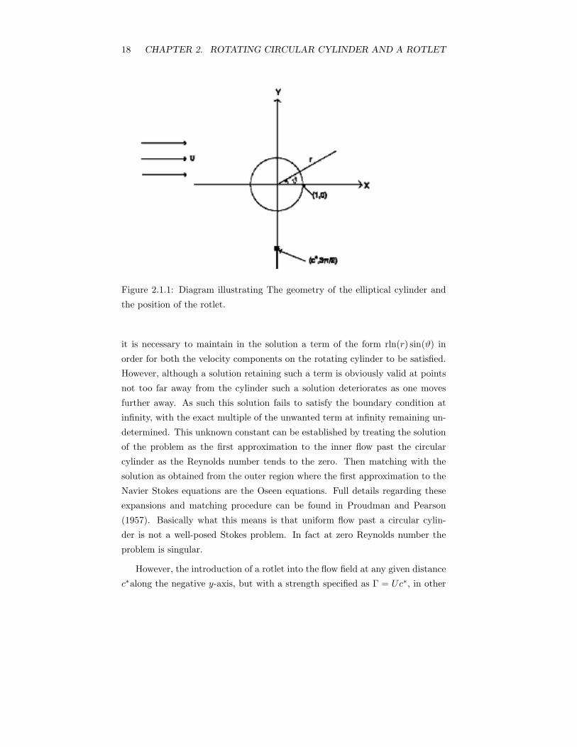
A study has been made of the flow generated by rotating a circular cylinder
within a uniform stream of viscous fluid in the presence of a line rotlet. With
the origin of the coordinates coinciding with the center of the cylinder, then the
polar coordinate system (r, ϑ) has the boundary of the cylinder at r = a and the
position of the rotlet at (c∗, 3π/2), as shown in Figure 2.1.1. There are four basic
parameters that occur in this problem, namely, the Reynolds number, defined as
Re = 2aU/ν, the rotational parameter α = aω0/U , the non dimensional length
c = c∗/a and the non dimensional strength of the rotlet β = Γ/Ua, where ν
is the coefficient of kinematic viscosity of the fluid, U the unperturbed main
stream speed, (the stream at infinity is assumed to flow parallel to the x-axis
in the positive x direction), ω0the angular velocity of the cylinder and Γ the
strength of the rotlet.
At zero Reynolds number the governing equation is the biharmonic equation.
In the absence of a rotlet no solution of this equation, which satisfies both the
boundary conditions on the cylinder and at infinity, is possible. This arises since
17
18 CHAPTER 2. ROTATING CIRCULAR CYLINDER AND A ROTLET
Figure 2.1.1: Diagram illustrating The geometry of the elliptical cylinder and
the position of the rotlet.
it is necessary to maintain in the solution a term of the form rln(r) sin(ϑ) in
order for both the velocity components on the rotating cylinder to be satisfied.
However, although a solution retaining such a term is obviously valid at points
not too far away from the cylinder such a solution deteriorates as one moves
further away. As such this solution fails to satisfy the boundary condition at
infinity, with the exact multiple of the unwanted term at infinity remaining un-
determined. This unknown constant can be established by treating the solution
of the problem as the first approximation to the inner flow past the circular
cylinder as the Reynolds number tends to the zero. Then matching with the
solution as obtained from the outer region where the first approximation to the
Navier Stokes equations are the Oseen equations. Full details regarding these
expansions and matching procedure can be found in Proudman and Pearson
(1957). Basically what this means is that uniform flow past a circular cylin-
der is not a well-posed Stokes problem. In fact at zero Reynolds number the
problem is singular.
However, the introduction of a rotlet into the flow field at any given distance
c∗along the negative y-axis, but with a strength specified as Γ = Uc∗, in other
2.1. INTRODUCTION 19
words with the parameter β = c, allows a solution to be obtained. analytical
solutions to this problem have been obtained by Dorrepaal, O,Neill and Ranger
(1984). Their work examines the flows generated in a fluid by the introduction
of a line singularity, such as a stokeslet or rotlet, in the presence of a circular
cylinder and shows that a phenomenon analogous to the Stokes paradox exists
in that flows with a uniform stream far from the cylinder may be produced.
As a consequence, the uniform streaming flow past a circular cylinder, when a
line stokeslet or rotlet of certain strength is present, is a well-posed problem in
Stokes flow.
The solution by Dorrepaal et al. (1984) employed an image type approach,
plus a clever and simplistic deduction, which enabled the result to be constructed
devoid of most of the analysis. However, the present work has established the
same solution by using a Fourier Series approach and has confirmed this numer-
ically by the application of a modification to the Boundary Element Method.
The latter appears to provide an approach for the solution of the biharmonic
equation, which requires only the position of the singularity, plus the physical
values of the drag, lift and the moment on the circular cylinder to be known.
In addition it seems capable of being extended to accommodate the presence
of several different bodies as well as allowing more complex shapes for which
an analytical solution is impossible. It is intended to show that the presence
of a rotlet in a uniform flow at non-zero Reynolds number allows an otherwise
singular problem to become well-posed as the Reynolds number becomes zero.
The main aim of this chapter is to solve numerically the Navier-Stokes equa-
tions for steady, two-dimensional, incompressible viscous fluid flow past a ro-
tating circular cylinder of radius a in the presence of a rotlet of strength Γ,
which is located at the point (r, ϑ) = (c∗, 3π/2), c∗ > a. At large distance from
the cylinder it is assumed that there is a uniform flow of speed U , which is
parallel to negative x-axis. Initially the strength of the rotlet is set to zero and
the problem solved with Reynolds numbers 5 and 20. The results are in very
good agreement with those obtained by Tang (1990). Using this as an initial
estimate of the solution when a line singularity is present an iterative technique
is developed in order to solve the problem when a rotlet, at (c∗, 3π/2), of small
strength is introduced into the flow. As the drag, lift and moment on the cir-
cular cylinder are the most important physical quantities, as well as being easy
to measure experimentally, Tang (1990), then in this work particular attention
20 CHAPTER 2. ROTATING CIRCULAR CYLINDER AND A ROTLET
has been paid to these quantities.
2.2 Basic Equations and the Boundary Condi-
tions
The origin of the coordinate system is fixed at the center of the circular cylinder
of radius a and the positive x-axis taken in the same direction as that of the
uniform flow at large distances from the cylinder. Polar coordinates (r, ϑ) are
chosen such that ϑ = 0 coincides with the positive x-axis,
x = rcos(ϑ) and y = rsin(ϑ). (2.2.1)
A line rotlet of strength Γ is located at the point r = c∗, ϑ = 3π/2, where c∗ > a.
The steady flow of an incompressible fluid in a fixed two-dimensional Cartesian
frame of reference can be described by the equations,
(u.∇)u = −1ρ∇p+ ν∇2u (2.2.2)
∇.u = 0 (2.2.3)
where u, ρ, p and ν are the velocity, density, pressure and the kinematic viscosity
of the fluid, respectively.
Applying the curl operator to equation (2.2.2) produces
(u.∇)ω = ν∇2ω (2.2.4)
where ω = ∇Xu .
In two-dimensional motion the polar resolute of u can be expressed in terms
of the stream function Ψ by
vr =1r
∂Ψ∂ϑ
, vϑ = −∂Ψ∂r
(2.2.5)
where vrand vϑare the velocity components in the r and ϑ directions, respec-
tively. By introducing the dimensionless variables
2.2. BASIC EQUATIONS AND THE BOUNDARY CONDITIONS 21
x′ = x/a, u′ = u/U,Ψ′ = Ψ/Ua and ω′ = ωa/U, (2.2.6)
then the governing equations in non-dimensional form become
∇2ω′ = −Re2∂(ψ′, ω′)∂(x′, y′)
(2.2.7)
∇2Ψ′ = −ω′ (2.2.8)
where ω′ and Ψ′ are the non-dimensional scalar vorticity and stream function,
respectively. For convenience the ′,s will from now on be removed. It is required
to solve equations (2.2.7) and (2.2.8) subject to the no-slip conditions imposed
by the circular cylinder, namely
Ψ = 0,∂ψ
∂r= −α on r = 1, 0 ≤ ϑ < 2π (2.2.9)
and the boundary conditions at large distances from the cylinder
∂ψ
∂r→ − sin(ϑ),
1r
∂ψ
∂ϑ→ cos(ϑ) as r → ∞, 0 ≤ ϑ < 2π (2.2.10)
In the presence of a line rotlet the stream function behaves as
Ψ ≈ −β lnR1 as R1 → 0 (2.2.11)
where R1measures the distance from the rotlet and is thus given by
R1 = (r2 + c2 + 2rc sin(ϑ))1/2, (2.2.12)
where (c, 3π/2) is the position of the rotlet.
In the above definition of the stream function the signs appearing in the
expressions in (2.2.5) are the opposite to those given by Dorrepaal et al. (1984)
but follow those adopted by Tang (1990) since it is a comparison with their
results at non zero Reynolds number that is to be undertaken.
22 CHAPTER 2. ROTATING CIRCULAR CYLINDER AND A ROTLET
For numerical convenience the perturbation stream function ψ is introduced
as
ψ = Ψ − y − βV, (2.2.13)
where V = ln(r2 + c2 + 2rcsin(ϑ))1/2with c = c∗/a and β = Γ/(Ua) being two
non-dimensional parameters. Expansion (2.2.13) has been taken so that ψ → 0
as r → ∞. If the parameter β = 0 then the problem reduces to that solved
by Tang (1990). However, with the Reynolds number equal to zero and the
parameter β = c then the situation is that studied by Dorrepaal et al. (1984)
except that the geometry in the present case corresponds to a rotation through
π/2 of their flow pattern. Hence, their stream is flowing along the negative
y-axis with their rotlet at (c∗, 0), whereas in the present geometry the stream
flows along the negative x-axis with the rotlet at (c∗, 3π/2).
Using expression (2.2.13) in equations (2.2.7) and (2.2.8) gives
∂2ω
∂r2+
1r
∂ω
∂r+
1r2∂2ω
∂ϑ2= −Re
2r(∂ψ
∂r
∂ω
∂ϑ− ∂ψ
∂ϑ
∂ω
∂r)
− Re
2r[∂ω
∂ϑ(sin(ϑ) + β
r + csin(ϑ)r2 + c2 + 2rcsin(ϑ)
]
+Re
2r[∂ω
∂r(rcos(ϑ) + β
rccos(ϑ)r2 + c2 + 2rcsin(ϑ)
]
(2.2.14)
∂2ψ
∂r2+
1r
∂ψ
∂r+
1r2∂2ψ
∂ϑ2= −ω (2.2.15)
respectively.
The boundary conditions (2.2.9) and (2.2.10) are then expressed in the form
ψ = − sin(ϑ) − β ln(1 + c2 + 2csin(ϑ))1/2 on r = 1, 0 < ϑ < 2π (2.2.16)
∂ψ
∂r= −α− sin(ϑ) − β(
1 + c sin(ϑ)1 + c2 + 2c sin(ϑ)
) on r = 1, 0 < ϑ < 2π, (2.2.17)
∂ψ
∂r=
1r
∂ψ
∂ϑ→ 0, as r → ∞, 0 ≤ ϑ < 2π. (2.2.18)
2.2. BASIC EQUATIONS AND THE BOUNDARY CONDITIONS 23
Filon (1926) showed that in the absence of any rotlet the asymptotic form for
the dimensional stream function at large distances from the cylinder and outside
the wake region is given by
ψ ≈ rsin(ϑ) +CL ln(r/a)
2π+CD(ϑ− π)
2π, as r → ∞, 0 < ϑ < 2π, (2.2.19)
where CL = L/(ρU 2a) and CD = D/(ρU2a), L and D being the lift and drag
on the cylinder . Imai (1951) found higher-order terms in this stream function
expansion and showed how the coefficients related to the moment on the cylin-
der. In the case of zero Reynolds number no solution of the equation ∇4Ψ = 0
is possible, which matches the free stream condition at infinity and satisfies the
boundary condition on r = 1. The solution, which satisfies the no slip condition
on the cylinder and tends to infinity most slowly as r → ∞ is
Ψ ≈ Asin(ϑ)[rln(r) − r/2 + 1/(2r)], (2.2.20)
which has been obtained by discarding the term involving r3. The non-dimensional
drag is directly related to the coefficient A, via the expression 4πA, but the solu-
tion suffers from the defect that it does not determine the value of the constant
A. The neglected inertial terms are of the order ((A)2 ln(r))/r2whilst the vis-
cous forces are of the order A/(Rer3) and these terms are of comparable order
when ARe(r ln(r))/a � 0(1). Hence, the Stokes solution should not be expected
to be valid beyond a value given by this expression. That is why the Stokes
solution may be an adequate representation of the fluid flow relatively close to
the cylinder but cannot represent a uniform approximation to the total velocity
distribution. However, it is possible to write the Stokes solution in the form
Ψ = A[(−rln(f(Re)) + rln(rf(Re))) − r/2 + 1/(2r)] sin(ϑ), (2.2.21)
where f(Re) is an arbitrary function of Re . For f(Re) << 1 and rf(Re)
of order unity, the dominant term is −A(ln(f(Re))rsin(ϑ). If this is to repre-
sent the external flow, namely a uniform stream Ursin(ϑ), then one must set
A = −1/ ln(f(Re)). By substituting this value of A and r = 1/f (Re) into
ARe(r ln(r))/a, one obtains
24 CHAPTER 2. ROTATING CIRCULAR CYLINDER AND A ROTLET
Re/f (Re) � 0(1). (2.2.22)
So for f(Re) = Re the Stokes solution leads to a uniform stream of order unity
in that region where the Stokes equation ceases to be valid . This suggests that
for small Reynolds number the external uniform stream condition is reached
before the Stokes approximation breaks down, so the Stokes flow represents the
solution in the inner region near the cylinder but the outer flow requires the
introduction of an Oseen variable and the procedure involves the matching of
the inner and outer expansions. This matching process leads to the obvious
linkage between the coefficients of the terms in Oseen’s expansion in the outer
region, closely related to Filon’s expansion, with those from the in the inner
region. Hence, the appropriate value of A can be obtained, as already indicated
from the solution in the outer region. Any similar term in a Stokes expansion,
such as a Brln(r) cos(ϑ) term in the stream function expansion, has its coefficient
similarly related to the lift. Solutions of the Stokes equation represented by the
form f(r) sin(ϑ) or g(r) sin(ϑ) fail to produce any moment contribution, but it
can easily be seen that the solution of ∇4Ψ = 0, which has a non-zero moment
arises from the ln(r/a) term. Using these results, it is possible from the Stokes
expansion far from the cylinder to establish both the force and the moment on
the cylinder. The Stokes solution produced by Dorrepaal, O,Neill and Ranger
(1984) is able to immediately produce the drag, lift and moment on the circular
cylinder from its expansion at large distances from the cylinder; although the
contribution from the singularity at the rotlet must first be removed from the
coefficient of the ln(r/a) term before it represents the moment on the cylinder.
Since the stream function and vorticity equations are both elliptical in nature
we should supply one condition for each of the variables rather than use directly
conditions (2.2.16), (2.2.17) and (2.2.18). It has been reported by Fornberg
(1980,1985)and Tang (1990) that the choice of the boundary condition for the
vorticity, ω, is not as sensitive as that for the stream function, ψ, and many
authors have paid particular attention to the boundary condition for ψ at large
distances from the cylinder.
In this work we use the technique described by Tang (1990) in order to avoid
having to enforce the boundary condition (2.2.19) at large distances from the
cylinder. We therefore introduce the transformation
2.2. BASIC EQUATIONS AND THE BOUNDARY CONDITIONS 25
ξ =1r, η =
2ϑπ
(2.2.23)
and
f(r, ϑ) = ψ(r, ϑ)/r, (2.2.24)
namely
f(ξ, η) = ξψ(ξ, η) (2.2.25)
Thus, we have f = 0 on ξ = 0(i.e. at r = ∞) and this requires no approximation
to be made for ψ at large distances from the cylinder.
With the transformation (2.2.23) then the solution domain (1 ≤ r <∞, 0 ≤ϑ < 2π) is transformed into a finite rectangular region in the (ξ, η) plane (0 ≤ξ < 1, 0 ≤ η < 4), see figure (2.2.1). Substituting expressions (2.2.23) and
(2.2.24) into the governing equations (2.2.14) and (2.2.15) one obtains
(2.2.26)
ξ3∂2f
∂ξ2− ξ2
∂f
∂ξ+
4ξπ2
∂2f
∂η2+ ξf = −ω (2.2.27)
and the boundary conditions (2.2.10) and (2.2.11) now become
f = − sin(πη/2) − β ln(1 + c2 +1/2 2csin(πη/2))
= fBonr = 1, 0 ≤ η < 4,(2.2.28)
∂f
∂ξ= α+ sin(πη/2) + β(
1 + csin(πη/2)1 + c2 + 2csin(πη/2)
)
= f ′B on r = 1, 0 ≤ η < 4,
(2.2.29)
f = 0, ω = 0, on ξ = 0, 0 ≤ η < 4. (2.2.30)
Further, since the solution is periodic in η we also require that
f(ξ, 4) = f(ξ, 0), ω(ξ, 4) = ω(ξ, 0), for 0 ≤ ξ ≤ 1, (2.2.31)
which along with all the other boundary conditions are indicated in figure 2.2.1.
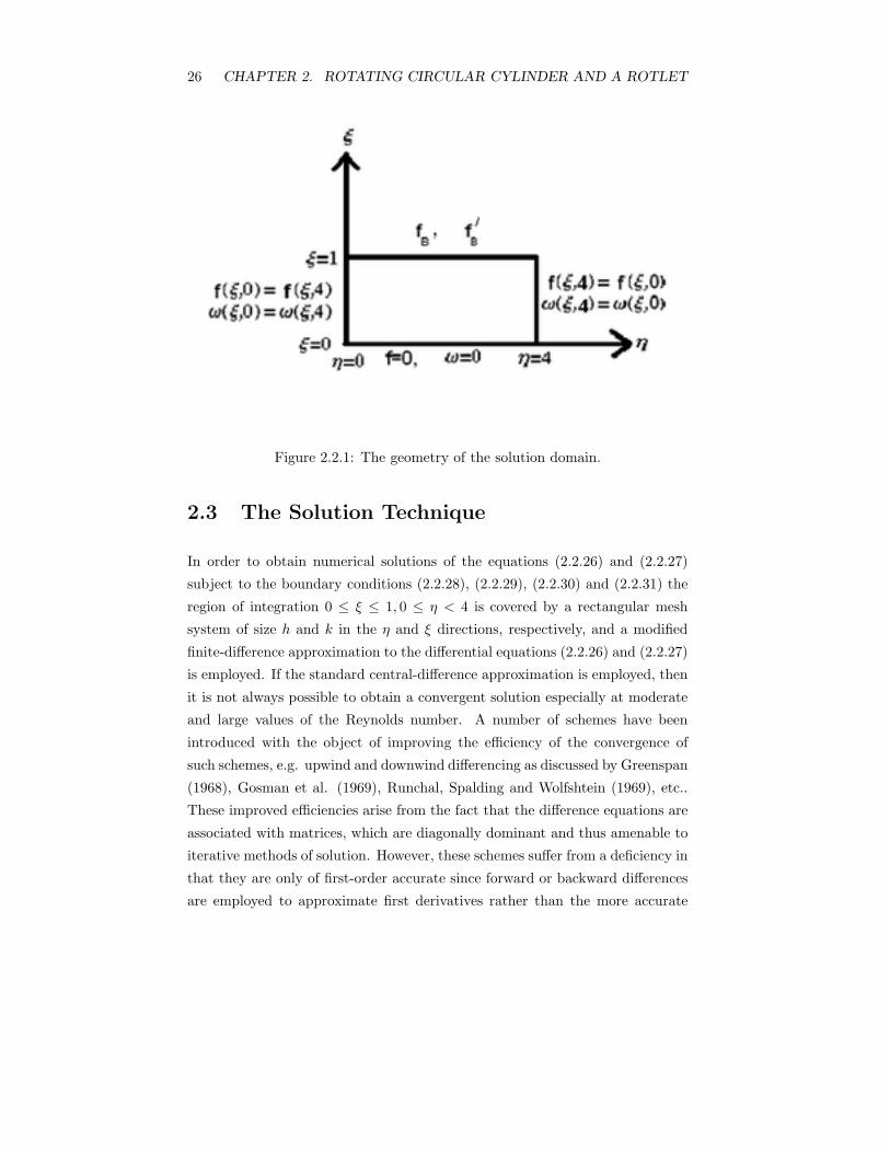
26 CHAPTER 2. ROTATING CIRCULAR CYLINDER AND A ROTLET
Figure 2.2.1: The geometry of the solution domain.
2.3 The Solution Technique
In order to obtain numerical solutions of the equations (2.2.26) and (2.2.27)
subject to the boundary conditions (2.2.28), (2.2.29), (2.2.30) and (2.2.31) the
region of integration 0 ≤ ξ ≤ 1, 0 ≤ η < 4 is covered by a rectangular mesh
system of size h and k in the η and ξ directions, respectively, and a modified
finite-difference approximation to the differential equations (2.2.26) and (2.2.27)
is employed. If the standard central-difference approximation is employed, then
it is not always possible to obtain a convergent solution especially at moderate
and large values of the Reynolds number. A number of schemes have been
introduced with the object of improving the efficiency of the convergence of
such schemes, e.g. upwind and downwind differencing as discussed by Greenspan
(1968), Gosman et al. (1969), Runchal, Spalding and Wolfshtein (1969), etc..
These improved efficiencies arise from the fact that the difference equations are
associated with matrices, which are diagonally dominant and thus amenable to
iterative methods of solution. However, these schemes suffer from a deficiency in
that they are only of first-order accurate since forward or backward differences
are employed to approximate first derivatives rather than the more accurate
2.3. THE SOLUTION TECHNIQUE 27
second-order central-difference formula. The formulation in which all derivatives
are approximated by central differences is of second-order accuracy but the
matrix associated with the difference equations may not be diagonally dominant.
The iterative procedures may be slowly convergent or even divergent when this
method is applied .
There are also finite-difference schemes, which are of second-order accuracy
and for which the associated matrices are always diagonally dominant. These
methods rely upon rather specialized forms of local approximations and yield
difference equations, which involve the exponential function. These schemes
were first introduced by Allen and Southwell (1955) in approximating the equa-
tion governing the vorticity during the course of finding numerical solutions for
the steady two-dimensional flow past a circular cylinder. Dennis and Hudson
(1978) showed that by a suitable adaptation of an alternative to the Allen and
Southwell method suggested by Dennis (1960), an approximation of second-
order accuracy, yielding difference equations with an associated matrix, which
is diagonally dominant, can be obtained. These difference equations do not
involve the exponential function and can be looked upon as a rather more com-
plicated version of the central-difference formulation. The Dennis and Hudson
method contains more terms in the finite-difference equations than the usual
central-difference approximation but the presence of these extra terms is very
important for the associated matrix to be diagonally dominant. Numerous au-
thors have performed several numerical experiments, which confirm that the
method by Dennis and Hudson succeeds where the standard central-difference
formulation fails, see Dennis (1960), Price, Varga and Warren, Nallasamy and
Krishna Prasad (1977) and Dennis and Hudson (1978). Thus, in this book a
modified version of the finite-difference approximation as described by Hudson
and Dennis, has been used.
It is found most convenient to set up a mesh system such that the mesh size in
both the ξ and η directions are k = h = 1/N , where N is a preassigned positive
integer. In view of the periodic conditions (2.2.31), an extra line of computation
η = 4 + h for 0 ≤ ξ ≤ 1 is introduced. Then we have (N + 1)x(M + 1) mesh
points, where M = 4N + 1, the mesh points (ξi, ηi)(0 ≤ i ≤ N, 0 ≤ j ≤ M)
are (ih, jh). If subscripts 0,1,2,3 and 4 denote quantities at the grid points
(ξ0, η0), (ξ0, η0 − h), (ξ0 + h, η0), (ξ0, η0 + h) and (ξ0 − h, η0), respectively, then
on using the Dennis and Hudson scheme, equations (2.2.26) and (2.2.27) may
28 CHAPTER 2. ROTATING CIRCULAR CYLINDER AND A ROTLET
be written in the form
(β∗2
2+
2π2ξ0
2 − h2
4ξ02 )f0 = (1
π2ξ02 )f1 + (
β∗2
4− β∗h
8ξ0)f2 + (
1π2ξ0
2 )f3
+ (β∗
4+β∗h8ξ0
)f4 + (h2
4ξ03 )ω0
(2.3.1)
(β∗2
2+
2π2ξ0
2 )ω0 = (1
π2ξ0− a(ξ0, η0) −D(ξ0, η0))ω1
+ (β∗2
4+ b(ξ0, η0) + E(ξ0, η0))ω2 + (
1π2ξ0
+ a(ξ0, η0) +D(ξ0, η0))ω3
+ (β∗
4− b(ξ0, η0) − E(ξ0, η0))ω4
(2.3.2)
with β∗ = hk
a(ξ0, η0) =Reh
8πξ02 (v0 +f0ξ0
+1ξ0
sin(ϑ)) (2.3.3)
b(ξ0, η0) = β(Reh
8πξ02u0 +h
8ξ0+Reh
16ξ0cos(ϑ)) (2.3.4)
D(ξ0, η0) = −βReh8πξ02 (
1 + cξ0 sin(ϑ)1 + c2ξ0
2 + 2cξ0 sin(ϑ)) (2.3.5)
E(ξ0, η0) = −βReh16
(c cos(ϑ)
1 + c2ξ02 + 2cξ0 sin(ϑ)
) (2.3.6)
where (u0, v0) are defined as
u0 =∂f(ξ0, η0)
∂η, v0 =
∂f(ξ0, η0)∂ξ
(2.3.7)
The standard central-difference approximations may be obtained by setting
the extra terms D(ξ0, η0), E(ξ0, η0) to be zero.
We now briefly outline how the boundary conditions (2.2.28)-(2.2.30) can be
implemented. The boundary condition for the vorticity on ξ = 1 can be found
by using Taylor expansion for f and ω and inserting in equation (2.2.27) to get
second-order accurate finite differences.

2.3. THE SOLUTION TECHNIQUE 29
boundary conditions for ω :
on ξ = 0, 0 ≤ η < 4 : i = 0, 0 ≤ j < M ; ω0j = 0;
on ξ = 1, 0 ≤ η < 4 : i = N, 0 ≤ j < M ; ω0j = ωnj ;(2.3.8)
ωnj = [(1 − h2
2− h3
6)fnj − f(n−1)j −
h2
6ω(n−1)j
− h(1 − h2
2− h3
6)f ′nj +
4h3
6π2(g2j − (1 +
3h
)g1j)]/(h2
3(1 + h))
(2.3.9)
with
f ′nj = α−
β(1 + csin(π2 ηj))
1 + c2 + 2csin(π2 ηj)
+β
2ln(1 + c2 + 2csin(
π
2ηj)) (2.3.10)
gij =π2
4sin(
π
2ηj) −
βπ2
4(csin(π
2 ηj(1 + c2) + 2c2)(1 + c2 + 2csin(π
2 ηj))2(2.3.11)
g2j = −βπ2c(3c+ c3 + (1 + 3c2)sin(π
2 ηj) − 2c3cos2(π2 ηj))
2(1 + c2 + 2csin(π2 ηj))3
(2.3.12)
on η = 4 + h, 0 ≤ ξ ≤ 1 : 0 ≤ i ≤ N, j = M ; ωim = ωi1; (2.3.13)
on η = 0, 0 ≤ ξ ≤ 1 : 0 ≤ i ≤ N, j = 0; ωi0 = ωim−1; (2.3.14)
boundary conditions for f :
on ξ = 0, 0 ≤ η < 4 : 0 ≤ j < M, i = 0; f0j = 0;
on ξ = 1, 0 ≤ η < 4 : 0 ≤ j < M, i = N ;(2.3.15)
fnj = − sin(π
2ηj) +
β
2ln(1 + c2 + 2csin(
π
2ηj)) (2.3.16)
on η = 4 + h, 0 ≤ ξ ≤ 1 : 0 ≤ i ≤ N, j = M ; fim = fi1; (2.3.17)
on η = 0, 0 ≤ ξ ≤ 1 : 0 ≤ i ≤ N, j = 0; fi0 = fim−1; (2.3.18)
30 CHAPTER 2. ROTATING CIRCULAR CYLINDER AND A ROTLET
The resulting finite-difference equations (2.3.1) and (2.3.2), subject to the bound-
ary conditions (2.3.8)-(2.3.18), were solved iteratively in a similar way to that
described by Tang (1990).
¿From equation (2.2.6) the non-dimensional speed of the uniform stream at
large distance from the cylinder is unity, whereas the non-dimensional strength
of the rotlet at the position (c, 3π/2), namely β, is variable. In order to compare
the results with Dorrepaal et al. (1984) the value of c is fixed at the magnitude
used in their calculations, namely c = 3.
Since the force components (drag and lift) and the moment are very sensitive
to the method of solution, particular attention has been given to these quantities.
If Fx and Fy are the dimensional drag and lift on the cylinder, then
Fx =∫ 2π
0
(σrr cos(ϑ) − σrϑ sin(ϑ))r=1 rdϑ (2.3.19)
Fy = −∫ 2π
0
(σϑr cos(ϑ) + σrr sin(ϑ))r=1 rdϑ (2.3.20)
Introducing the constitutive relations
σrr = −p+ 2μ∂Vr
∂r, (2.3.21)
σrϑ = σϑr = μ(r∂
∂r(Vϑ
r) +
1r
∂Vr
∂ϑ), (2.3.22)
σϑϑ = −p+ 2μ(1r
∂Vϑ
∂ϑ+Vr
r), (2.3.23)
into expressions (2.3.19) and (2.3.20) results in
Fx =∫ 2π
0
r[∂p
∂ϑ− 2μ
1r
∂
∂r(∂2Ψ∂ϑ2
+ Ψ) + μ∇2Ψ] sin(ϑ)dϑ, (2.3.24)
Fy = −∫ 2π
0
r[∂p
∂ϑ− 2μ
1r
∂
∂r(∂2Ψ∂ϑ2
+ Ψ) + μ∇2Ψ] cos(ϑ)dϑ, (2.3.25)
Using the ϑ component of the Navier Stokes equations, namely
2.3. THE SOLUTION TECHNIQUE 31
1r(∂p
∂ϑ) = −μ∂∇
2Ψ∂r
(2.3.26)
and substituting ∇2Ψ = −ω, which is equation (2.2.8) but in its dimensional
form, the equations (2.3.24) and (2.3.25) can be written in the form
Fx = μ
∫ 2π
0
r[r∂ω
∂ϑ− ω − 2
r
∂
∂r(∂2Ψ∂ϑ2
+ Ψ)] sin(ϑ)dϑ, (2.3.27)
Fy = −μ∫ 2π
0
r[r∂ω
∂ϑ− ω − 2
r
∂
∂r(∂2Ψ∂ϑ2
+ Ψ)] cos(ϑ)dϑ, (2.3.28)
The above expressions are still dimensional, but defining the
lift and the drag coefficients by
CD = Fx/(ρU2a) and CL = Fy/(ρU2a) (2.3.29)
enables CDand CLto be written as
CD =2Re
∫ 2π
0
r[r∂ω
∂ϑ− ω − 2
r
∂
∂r(∂2Ψ∂ϑ2
+ Ψ)] sin(ϑ)dϑ, (2.3.30)
CL = − 2Re
∫ 2π
0
r[r∂ω
∂ϑ− ω − 2
r
∂
∂r(∂2Ψ∂ϑ2
+ Ψ)] cos(ϑ)dϑ, (2.3.31)
where r,Ψ and ω are all non-dimensional.
In terms of the independent variables ζ and ϑ,CD and CL become
CD =2Re
∫ 2π
0
[− ∂ξ
∂ϑ− ω − 2
∂
∂ξ(∂2Ψ∂ϑ2
+ Ψ)] sin(ϑ)dϑ, (2.3.32)
CL = − 2Re
∫ 2π
0
[−∂ω∂ϑ
− ω − 2∂
∂ξ(∂2Ψ∂ϑ2
+ Ψ)] cos(ϑ)dϑ, (2.3.33)
When the boundary conditions on the cylinder are introduced expressions (2.3.32)
and (2.3.33) reduce to those given by Tang (1990), except for a reversal of the
sign in CL and the omission of a factor 2 in the definition of both CL and CD.
32 CHAPTER 2. ROTATING CIRCULAR CYLINDER AND A ROTLET
The moment on the cylinder
M =∫ 2π
0
rσrϑrdϑ (2.3.34)
becomes, in dimensional form, on substituting the appropriate constitutive equa-
tion
M = −μ∫ 2π
0
r2[∂2ψ
∂r2− 1r
∂ψ
∂r− 1r2∂2Ψ∂ϑ2
] dϑ. (2.3.35)
Introducing the moment coefficient defined by
CM = M/(ρU 2a2) (2.3.36)
results in the non dimensional expression
CM =2Re
∫ 2π
0
r2[ω +2r
∂ψ
∂r+
2r2∂2Ψ∂ϑ2
] dϑ. (2.3.37)
In terms of the independent variables ξ and ϑ the moment coefficient becomes
CM =2Re
∫ 2π
0
[ω − 2∂ψ
∂ξ+ 2
∂2Ψ∂ϑ2
] dϑ, (2.3.38)
and the boundary conditions on the cylinder reduce this expression to
CM =2Re
∫ 2π
0
[ω − 2ω0] dϑ. (2.3.39)
Formulas (2.3.32), (2.3.33) and (2.3.39) are evaluated using Simpson’s rule. Due
to the need to evaluate the drag, lift and moment when Re = 0 we will work
with the non-dimensional quantities ReCD/2, ReCL/2 and ReCM/2 from now
on, namely Fx/(μU), Fy/(μU) and M/(μUa). However, when the Reynolds
number vanishes, that is the independence of the mainstream at infinity from
the strength of the rotlet is no longer valid, then when discussing an iterative
scheme in the following results section it is necessary to redefine the above three
quantities as (Fxa)/(μΓ), (Fya)/(μΓ) and M/(μΓ).
2.4. RESULTS 33
2.4 Results
Before we undertake a detailed discussion of the results it is important to stress
from Dorrepaal et al. (1984), and from our own investigation, that at Re = 0
it is impossible to obtain a solution for an arbitrary value of the parameter β,
which is contrary to what occurs at non zero Reynolds numbers. In the Re = 0
situation there is only one unique value of β, which will produce the uniform
stream at infinity, and the difficulty numerically is to achieve some mechanism,
which will enable the numerical method to converge to this quantity. Since
Stokes flow with a uniform flow at infinity means that the body must be free
of any force one can develop an iterative numerical scheme based upon this
fact to enable the unique value of β and the corresponding flow solution to be
determined. Exactly how this is achieved will be discussed in detail later within
this section. In order to compare the results obtained by the present numerical
method with those obtained previously, the values of the Reynolds number
Re = 5 and Re = 20, together with the absence of any rotlet (β = 0) and
with the rotational parameter α = 0, 0.5, 1 and 2, were initially investigated.
Solutions are obtained for the mesh sizes h = 1/10, 1/15, 1/20 and 1/40. In
Tang (1990), at both the above Reynolds numbers, repeated extrapolation of
results derived from h2extrapolation of the results from h = 1/10, 1/15, 1/20
and 1/40 produced only a 0.1% change in the coefficients of the lift and the
drag when compared with the values derived directly from using h = 1/40.
As a consequence it is proposed not to implement extrapolation but instead to
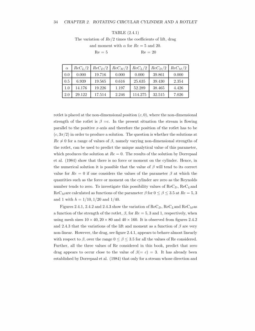
utilize a small value of h, namely h = 1/40. Values of Re/2 times the coefficients
of the lift, drag and moment are presented in table (2.4.1). The lift and drag
coefficients are in good agreement with those produced by Tang (1990).
At this stage, having established that the numerical procedure is produc-
ing the correct results for Re = 0 and α = 0, then the condition β = 0 is
relaxed. However, since the interest is in whether the problem is well posed as
the Reynolds number tends to zero, it is proposed to set α to be zero in the
remainder of the calculations to be presented in this chapter. Although such a
restriction can easily be removed if required.
It has already been established analytically by Dorrepaal et al. (1984) that
at Re = 0a solution in which there is a uniform stream of unit non-dimensional
strength flowing parallel to the positive y-axis is possible provided that the
34 CHAPTER 2. ROTATING CIRCULAR CYLINDER AND A ROTLET
TABLE (2.4.1)
The variation of Re/2 times the coefficients of lift, drag
and moment with α for Re = 5 and 20.
Re = 5 Re = 20
α ReCL/2 ReCD/2 ReCM/2 ReCL/2 ReCD/2 ReCM/2
0.0 0.000 19.716 0.000 0.000 39.861 0.000
0.5 6.939 19.565 0.616 25.635 39.430 2.354
1.0 14.176 19.226 1.197 52.289 38.465 4.426
2.0 29.122 17.514 2.246 114.275 32.515 7.026
rotlet is placed at the non-dimensional position (c, 0), where the non-dimensional
strength of the rotlet is β =c. In the present situation the stream is flowing
parallel to the positive x-axis and therefore the position of the rotlet has to be
(c, 3π/2) in order to produce a solution. The question is whether the solutions at
Re = 0 for a range of values of β, namely varying non-dimensional strengths of
the rotlet, can be used to predict the unique analytical value of this parameter,
which produces the solution at Re = 0. The results of the solution by Dorrepaal
et al. (1984) show that there is no force or moment on the cylinder. Hence, in
the numerical solution it is possible that the value of β will tend to its correct
value for Re = 0 if one considers the values of the parameter β at which the
quantities such as the force or moment on the cylinder are zero as the Reynolds
number tends to zero. To investigate this possibility values of ReCD, ReCLand
ReCMare calculated as functions of the parameter β for 0 ≤ β ≤ 3.5 at Re = 5, 3
and 1 with h = 1/10, 1/20 and 1/40.
Figures 2.4.1, 2.4.2 and 2.4.3 show the variation of ReCD, ReCLand ReCMas
a function of the strength of the rotlet, β, for Re = 5, 3 and 1, respectively, when
using mesh sizes 10× 40, 20× 80 and 40× 160. It is observed from figures 2.4.2
and 2.4.3 that the variations of the lift and moment as a function of β are very
non-linear. However, the drag, see figure 2.4.1, appears to behave almost linearly
with respect to β, over the range 0 ≤ β ≤ 3.5 for all the values of Re considered.
Further, all the three values of Re considered in this book, predict that zero
drag appears to occur close to the value of β(= c) = 3. It has already been
established by Dorrepaal et al. (1984) that only for a stream whose direction and
2.4. RESULTS 35
magnitude are related to the position and strength of the rotlet will a solution
be possible when Re = 0. In this case only for the specific value of β = c will
the problem be well posed and produce a solution for which the values for the
drag, lift and moment on the cylinder are all zero. For all other values of β
one will have the force and moment dependent on this parameter. It has been
shown elsewhere that when Re = 0 non-zero values of the drag and lift implies
that there are terms of the type rln(r) sin(ϑ) and rln(r) cos(ϑ) at large values of
r. Similarly non zero values of the moment requires a ln(r) term. Obviously the
presence of such terms violates the boundary condition that f = 0 as r → ∞,
and it is only when all such terms are absent that one will achieve the required
solution. This is why at Re = 0 it is impossible to obtain a convergent solution
for an arbitrary value of β, unlike the situation at Re = 0.
However, for Re = 0 one can think of the lift, drag and moment as functions
of β and only when these quantities acquire the value of zero will β achieve
its required value, namely β = c, and produce a convergent solution. Hence,
the technique adopted was that of a Newton Raphson iteration on CD(β). The
choice of CD, rather than CLor CMbeing based upon the linearity of this expres-
sion with respect to β, compared with the rather complex behavior of the latter
two quantities when considered as functions of this variable. The governing par-
tial differential in finite-difference form, namely equations (2.3.1) and (2.3.2),
were solved for two values of β, say β1and β2, the number of iterations being
terminated after a prescribed number since due to the boundary condition posed
at ξ = 0 convergent solutions are impossible. The resulting two non-zero values
of CD(β1) and CD(β2) are the values used in the Newton Raphson method in
order to establish a new value of β, say β3, at which CD(β3) is estimated to be
zero. Resolving for this new value of β, and using CD(β3) together with CD(β1),
or CD(β2), whichever is closest to zero, to produce from the Newton Raphson
solution a new value of β. The whole process is continued until the value of
CD(β3) reaches zero to within the required tolerance need to state what this is.
The value of β automatically results in the correct values of CLand CM . The
whole iterative procedure could equally well have been applied to setting either
the values of CL(β) or CM (β) to zero. The resulting value of β achieved by
this process was 3.0004, 3.0005 and 3.0010 for the mesh sizes 40 × 160, 20 × 80
and 10 × 40 respectively, compared with the exact analytical value of 3. The
streamline and vorticity patterns produced from the numerical computation and
36 CHAPTER 2. ROTATING CIRCULAR CYLINDER AND A ROTLET
shown in figures 2.4.4 (a) and 2.4.5 (a) are identical with those obtained from
the analytical solution.
Figure 2.4.4 show the streamline pattern obtain for β = 3 and Re = 0, 1, 3
and 5 for fine mesh size 40× 160. In this figure the affect of changing Reynolds
number it appear to be slight, but if we compare this figure by figure 2.4.8 the
affect of Reynolds number become more clear. The region include the rotlet
causes the separating streamline to close nearer the body.
Figure 2.4.5 show the vorticity pattern for β = 3 and Re = 0, 1, 3 and 5 for
40 × 160. The affect of changing Reynolds number not clear, since Reynolds
number is very small and the strength of the rotlet is very strong.
Figure 2.4.6 show the streamline pattern for β = 1.5 and Re = 1, 3 and 5.
The region include the rotlet becomes shorter but it appear to be unaffected by
the small change in the Reynolds number.
Figure 2.4.7 show the vorticity pattern for β = 1.5 and Re = 1, 3 and 5.
We note a slight movement of the line for equal vorticity. The vorticity in this
outer area is almost constant and the point wise change is much smaller than
the movement would seem to suggest.
Figure 2.4.8 shows the affect of the strength of the rotlet and how the result
it tends to result obtained by Tang (1984). Figure 2.4.8 (f) is identical with the
figure obtained by Tang (1990).
2.5 Conclusion
Numerical solutions of the full, steady, two-dimensional Navier-Stokes equations
have been obtained for the fluid flow past a circular cylinder for Reynolds num-
bers Re = 1, 3, 5 and 20 and rotational parameter 0 ≤ α ≤ 2 when a rotlet of
any given strength is placed at various positions outside the cylinder. Although
numerical solutions can be found for any value of the Reynolds number greater
than zero it is well known that when the Reynolds number is zero that a solution
only exists provided there is a relationship between the strength of the rotlet and
its location. Further, when the Reynolds number is zero the analytical solutions
are such that the drag, lift and moment are all identically zero. Therefore in
this chapter we have concentrated on obtaining numerical results with the drag,
lift and moment zero and developed a technique for extrapolating the results
obtained at small values of the Reynolds number to predict the solution for zero
2.5. CONCLUSION 37
Reynolds number. Using this technique it is found that the numerical results
are in excellent agreement with all the available theoretical results. We conclude
that the technique developed in this chapter may be used with confidence to
predict solutions for flows at zero Reynolds numbers for situations where there
are no analytical solutions.
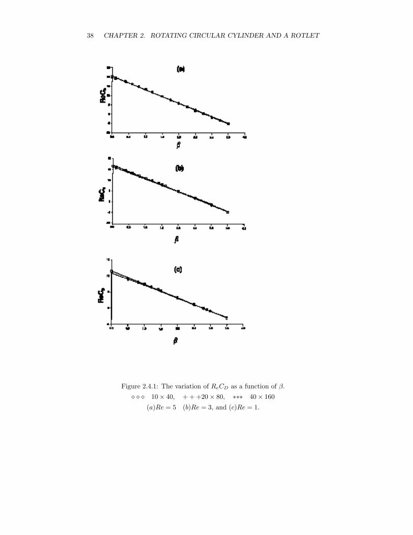
38 CHAPTER 2. ROTATING CIRCULAR CYLINDER AND A ROTLET
Figure 2.4.1: The variation of ReCD as a function of β.
10 × 40, + + +20 × 80, ∗∗∗ 40 × 160
(a)Re = 5 (b)Re = 3, and (c)Re = 1.
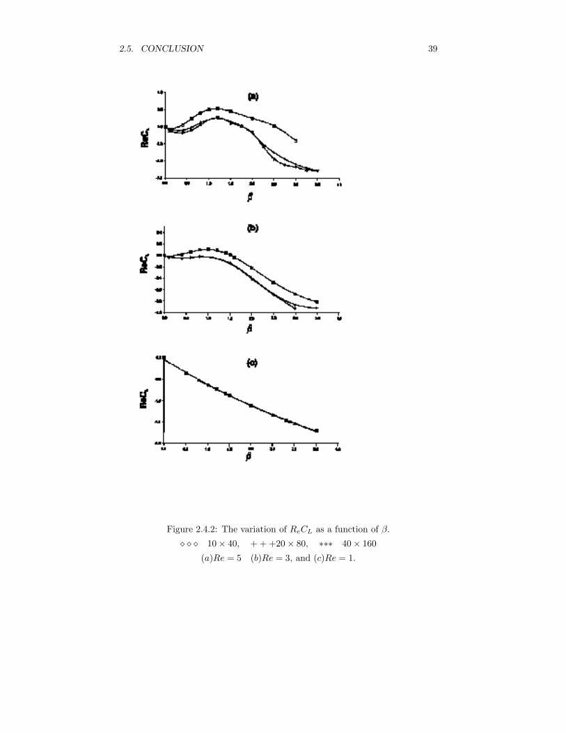
2.5. CONCLUSION 39
Figure 2.4.2: The variation of ReCL as a function of β.
10 × 40, + + +20 × 80, ∗∗∗ 40 × 160
(a)Re = 5 (b)Re = 3, and (c)Re = 1.
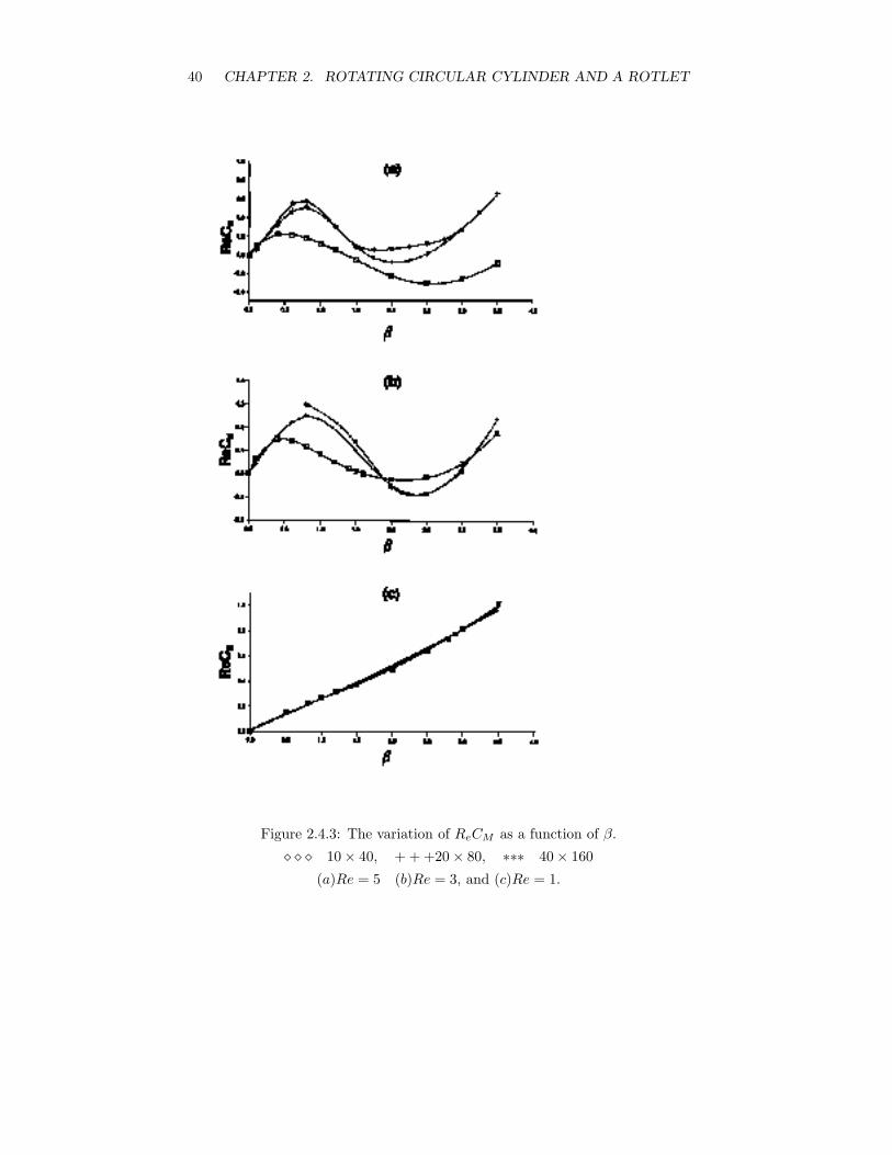
40 CHAPTER 2. ROTATING CIRCULAR CYLINDER AND A ROTLET
Figure 2.4.3: The variation of ReCM as a function of β.
10 × 40, + + +20 × 80, ∗∗∗ 40 × 160
(a)Re = 5 (b)Re = 3, and (c)Re = 1.
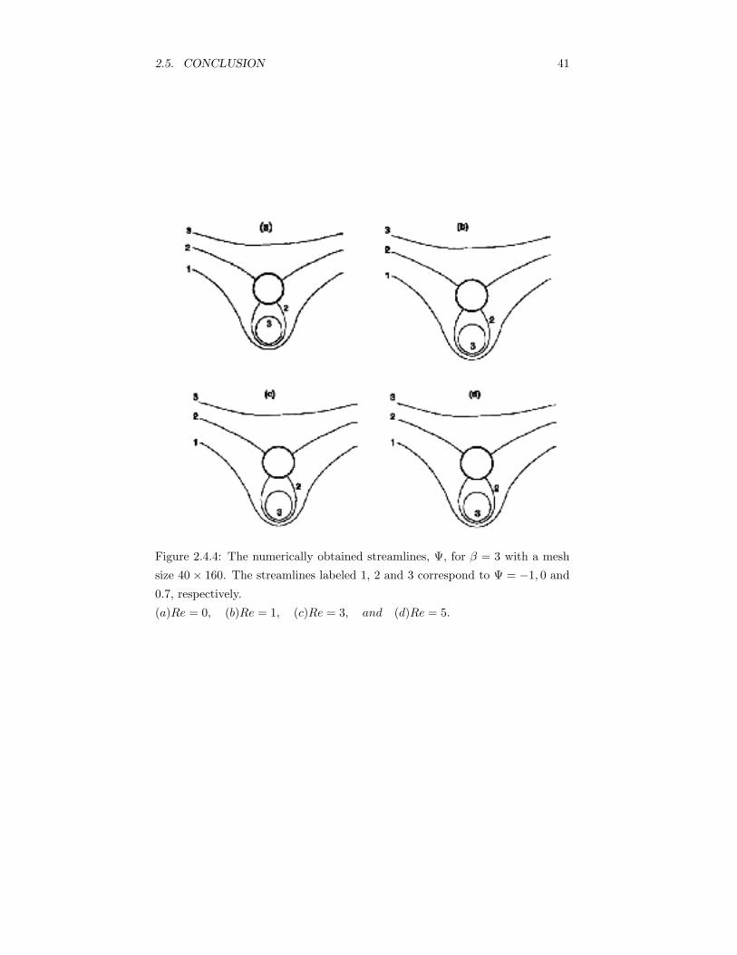
2.5. CONCLUSION 41
Figure 2.4.4: The numerically obtained streamlines, Ψ, for β = 3 with a mesh
size 40 × 160. The streamlines labeled 1, 2 and 3 correspond to Ψ = −1, 0 and
0.7, respectively.
(a)Re = 0, (b)Re = 1, (c)Re = 3, and (d)Re = 5.
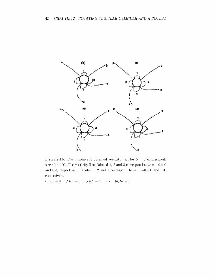
42 CHAPTER 2. ROTATING CIRCULAR CYLINDER AND A ROTLET
Figure 2.4.5: The numerically obtained vorticity , ω, for β = 3 with a mesh
size 40 × 160. The vorticity lines labeled 1, 2 and 3 correspond to ω = −0.4, 0
and 0.4, respectively. labeled 1, 2 and 3 correspond to ω = −0.4, 0 and 0.4,
respectively.
(a)Re = 0, (b)Re = 1, (c)Re = 3, and (d)Re = 5.
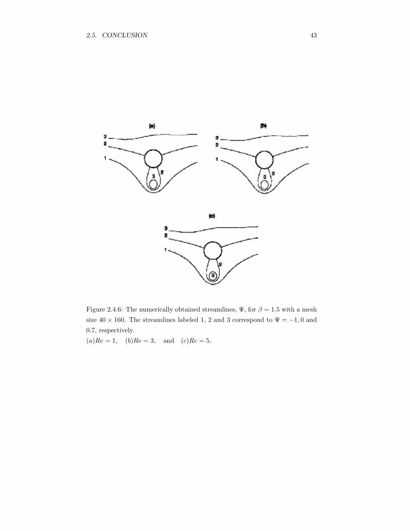
2.5. CONCLUSION 43
Figure 2.4.6: The numerically obtained streamlines, Ψ, for β = 1.5 with a mesh
size 40 × 160. The streamlines labeled 1, 2 and 3 correspond to Ψ = −1, 0 and
0.7, respectively.
(a)Re = 1, (b)Re = 3, and (c)Re = 5.
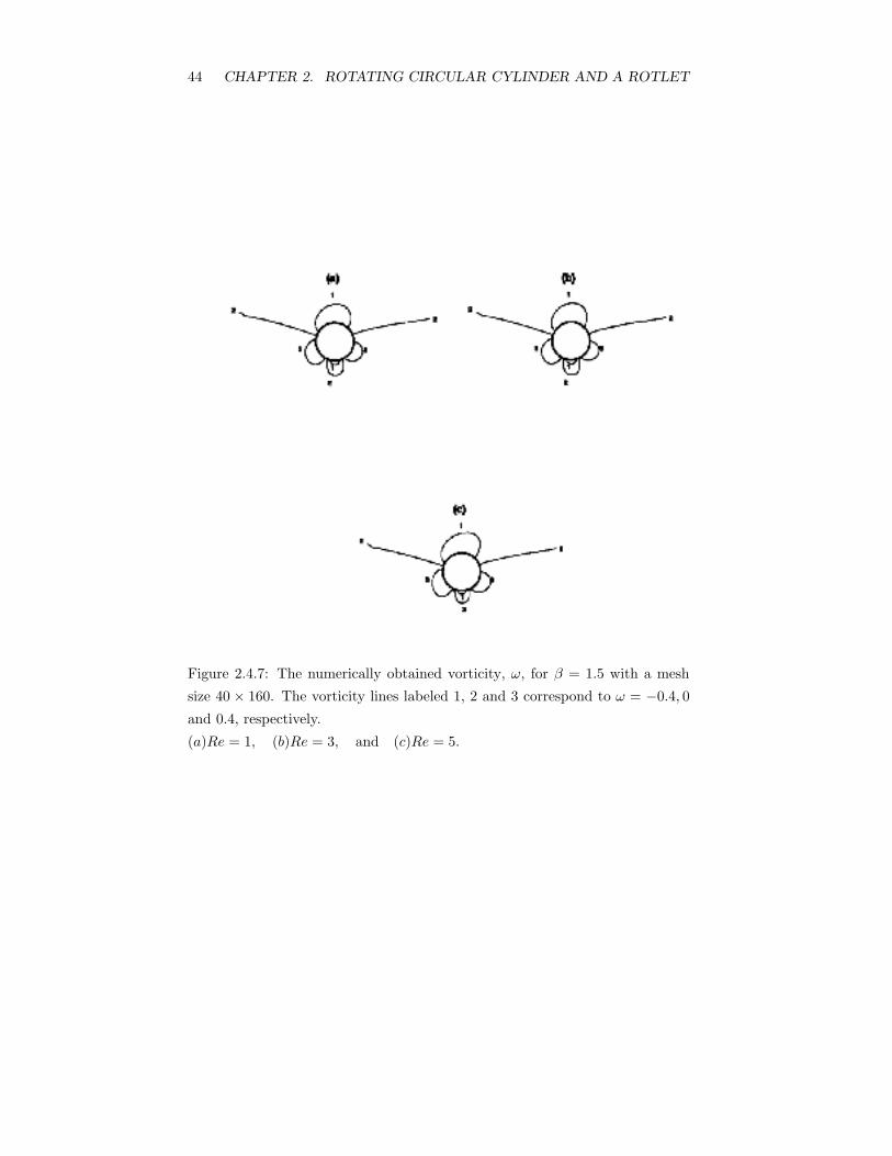
44 CHAPTER 2. ROTATING CIRCULAR CYLINDER AND A ROTLET
Figure 2.4.7: The numerically obtained vorticity, ω, for β = 1.5 with a mesh
size 40 × 160. The vorticity lines labeled 1, 2 and 3 correspond to ω = −0.4, 0
and 0.4, respectively.
(a)Re = 1, (b)Re = 3, and (c)Re = 5.
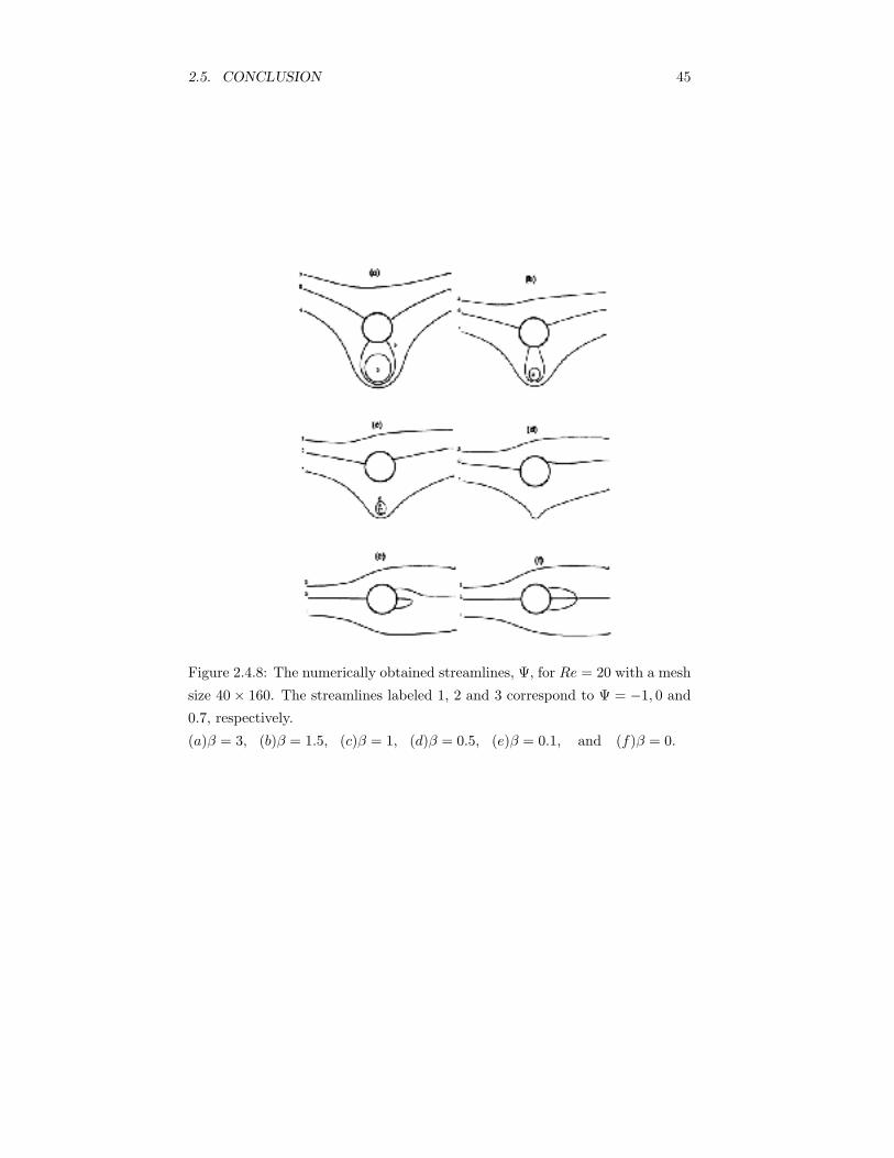
2.5. CONCLUSION 45
Figure 2.4.8: The numerically obtained streamlines, Ψ, for Re = 20 with a mesh
size 40 × 160. The streamlines labeled 1, 2 and 3 correspond to Ψ = −1, 0 and
0.7, respectively.
(a)β = 3, (b)β = 1.5, (c)β = 1, (d)β = 0.5, (e)β = 0.1, and (f)β = 0.

Chapter 3
ANALYTICAL SOLUTION
3.1 Solution Using Fourier Series
In this section the problem originally discussed by Dorrepaal, O’Neill and Ranger
(1984), namely that of a rotlet of non dimensional unit strength placed at a non
dimensional distance c, where c > 1, from a cylinder whose radius a has been
used as the non-dimensional length scale is investigated by an alternative ap-
proach. With the origin of the coordinates coinciding with the center of the
cylinder, then the non-dimensional polar coordinate system (r, ϑ), where
x = r cosϑ and y = r sinϑ, (3.1.1)
has the boundary of the cylinder at r = 1 and the position of the rotlet at (c, 0),
as shown in Figure 3.1.1. Since the equations to be considered are those arising
for two dimensional Stokes flow, then the elimination of the pressure terms from
these equations, together with the introduction of a non dimensional stream
function ψ, results in the biharmonic equation being the governing equation.
In the present approach it is required to solve the biharmonic equation
∇4ψ = 0 (3.1.2)
for the stream function ψ(r, ϑ), where r ≥ 1 and ∇2is the standard Laplacian
operator. The no slip and no normal flow boundary conditions imposed by the
circular cylinder are
47
48 CHAPTER 3. ANALYTICAL SOLUTION
Figure 3.1.1: Position of circular cylinder and rotlet.
ψ =∂ψ
∂r= 0, on r = 1. (3.1.3)
At present there appears no obvious condition to impose at infinity on the
flow developed locally by a rotlet placed outside a cylinder. However, without
any restrictions whatsoever then there are an infinite number of possibilities. As
such if one is to allow for the locally generated flows at infinity to be present,
then it appears realistic to assume that the flow which is established there is
that with the slowest possible growth rate. This would seem plausible due to
such a solution requiring the least amount of energy.
Before embarking on the present approach a few words relating to the solu-
tion by Dorrepaal, O’Niell and Ranger (1984) ought to be included due to its
relatively clever and simplistic nature. The knowledge that the solution of the
3.1. SOLUTION USING FOURIER SERIES 49
biharmonic equation can be expressed as the sum of two solutions of Laplace’s
equation, namely
ψ = φ1 + (r2 − 1)φ2, (3.1.4)
where φ1and φ2are harmonic functions, enabled the function φ1to be taken as
the potential solution for the flow due to a rotlet or stokelet outside a circular
cylinder. This means that the function φ1satisfies the constant stream function
condition on the boundary due to being formed from the singularity itself and
the two images inside the cylinder at the image point and the origin. The choice
of (r2 − 1) multiplying the harmonic function φ2results in the stream function
maintaining its constant value on the boundary of the cylinder. Hence, the
only requirement still outstanding in order to determine the complete solution
is that on the boundary of the cylinder the normal derivative of (r2 − 1)φ2is
the negative of the normal derivative of φ1. This usage of (r2 − 1), instead of
the usual r2, results in the above reducing to the necessity of find an harmonic
function φ2whose value on r = 1 is half the known normal derivative of φ1there.
It is this neat argument that enables the construction of the solution
ψ = ln(R1) − ln(R2c) + ln(r) +(r2 − 1)(rc cos ϑ− 1)
R22c
2, (3.1.5)
from what appears at first glance to be void of any analysis, where R1 and R2
are the distances from the rotlet and the image rotlet in the cylinder, and are
given by
R1 = (r2 + c2 − 2rccosϑ)1/2 (3.1.6)
and
R2 = (r2 +1c2
− 2r
ccosϑ)1/2 (3.1.7)
respectively. The present method is a more routine and less sophisticated ap-
proach than that mentioned above, however it follows a similar method but
without the clever insight. Initially the value of ψ is expressed as
ψ = ψ1 + ψ2, (3.1.8)
50 CHAPTER 3. ANALYTICAL SOLUTION
where ψ1 is the stream function corresponding to a single rotlet at (c, 0) and
ψ2is the change caused to this flow due to the presence of the cylinder and is
free of any singularities in the region r > 1. The expression for ψ1
ψ1 =12
ln(r2 + c2 − 2rccosϑ) (3.1.9)
is obviously an even function in ϑ and following Oberhettinger (1973) can be
expressed as a Fourier Series representation, namely
ln(c) −∞∑
n=1
rn
ncncos(nϑ) 1 ≤ r ≤ c. (3.1.10)
The restriction on the domain of r is due to the series being convergent only for
r ≤ c. Using the result that the general solution of
∇4ψ2 = 0, (3.1.11)
can be written as ψ2 = φ1 + r2φ2, where φ1 and φ2 are harmonic functions,
enables ψ2 to be expressed as
ψ2 = c0 +∞∑
n=1
(bn sin(nϑ) + cn cos(nϑ))/rn
+ r2d0 +∞∑
n=1
(an sin(nϑ) + dn cos(nϑ))/r(n−2).
(3.1.12)
Obviously, the lowest positive power of r in the choice of φ1 and φ2is taken
subject to being able to find a ψ which satisfies the boundary conditions on
r = 1, and hence produces the solution with the slowest possible growth as
r → ∞ . Applying the boundary conditions given by expressions (3.1.3) results
in
c0 = − ln c, d0 = 0
a1 = b1 = c1 = 0, d1 =12
an = bn = 0, cn =1cn
(1n− 1), dn =
1cn, n ≥ 1.
(3.1.13)
3.2. FORCES AND MOMENT ON THE CYLINDER 51
The series in expression (3.1.12) can now be summed to produce the result
obtained by Dorrepaal, O’Neill and Ranger (1984), namely expression (3.1.5).
Using the relationship between the vorticity ω and the stream function ψ,
ω = ∇2ψ (3.1.14)
establishes the vorticity as
ω =4c[r cosϑR2
2
− 2r(rc cos ϑ− 1)(rc− cosϑ)R4
2c2
+(rc cos ϑ− 1)
cR22
]. (3.1.15)
As the biharmonic equation and the boundary conditions are linear then the
modification of the problem to accommodate the circular cylinder rotating with
a non-dimensional clockwise angular velocity α, instead of being at rest, can
easily be achieved by the addition of the term α ln(r) to expression (3.1.5).
This is possible since ln(r) is a solution of the biharmonic equation and satisfies
the boundary conditions
vr = −1r
∂ψ
∂ϑ= 0 and vϑ =
∂ψ
∂r= α on r = 1. (3.1.16)
Hence, the stream function becomes
ψ = ln(R1) − ln(R2c) + ln(r) +(r2 − 1)(rc cos ϑ− 1)
R22c
2+ α ln(r), (3.1.17)
whilst the vorticity remains unchanged.
3.2 Forces and Moment on the Cylinder
The components of force (Fx, Fy) and the moment M acting on a volume of
fluid V surrounded by the surface S can be expressed as
Fx =∫
S
(σxxnx + σxyny)dS, (3.2.1)
Fy =∫
S
(σyxnx + σyyny)dS, (3.2.2)
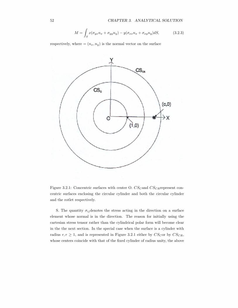
52 CHAPTER 3. ANALYTICAL SOLUTION
M =∫
S
x(σyxnx + σyyny) − y(σxxnx + σxyny)dS, (3.2.3)
respectively, where = (nx, ny) is the normal vector on the surface
Figure 3.2.1: Concentric surfaces with center O. CSCand CSCRrepresent con-
centric surfaces enclosing the circular cylinder and both the circular cylinder
and the rotlet respectively.
S. The quantity σijdenotes the stress acting in the direction on a surface
element whose normal is in the direction. The reason for initially using the
cartesian stress tensor rather than the cylindrical polar form will become clear
in the the next section. In the special case when the surface is a cylinder with
radius r, r ≥ 1, and is represented in Figure 3.2.1 either by CSCor by CSCR,
whose centers coincide with that of the fixed cylinder of radius unity, the above
3.2. FORCES AND MOMENT ON THE CYLINDER 53
expressions can be written as
Fx =∫
S
(σrr cosϑ− σrϑ sinϑ)rdϑ, (3.2.4)
Fy =∫
S
(σϑr cosϑ+ σrr sinϑ)rdϑ, (3.2.5)
M =∫
S
rσrϑrdϑ. (3.2.6)
Introducing the constitutive relations
σrr = −p+ 2μ∂Vr
∂r, (3.2.7)
σrϑ = σϑr = μ{r ∂∂r
(Vϑ
r) +
1r
∂Vr
∂ϑ}, (3.2.8)
σϑϑ = −p+ 2μ{1r
∂Vϑ
∂ϑ+Vr
r}, (3.2.9)
into expressions (3.2.4), (3.2.5) and (3.2.6) results in
Fx =∫ 2π
0
r[∂p
∂ϑ+ 2μ
1r
∂
∂r{∂
2ψ
∂ϑ2+ ψ} − μ∇2ψ] sinϑdϑ, (3.2.10)
Fy = −∫ 2π
0
r[∂p
∂ϑ+ 2μ
1r
∂
∂r{∂
2ψ
∂ϑ2+ ψ} − μ∇2ψ] cosϑdϑ, (3.2.11)
M = μ
∫ 2π
0
r2[∂2ψ
∂r2− 1r
∂ψ
∂r− 1r2∂2ψ
∂ϑ2]dϑ. (3.2.12)
On using the equations of motion, namely Stokes Equation, and the vorticity,
the equations (3.2.10) − (3.2.12 can be written in the form
Fx = μ
∫ 2π
0
r[r∂ω
∂r− ω +
2r
∂
∂r(∂2ψ
∂ϑ2+ ψ)] sin(ϑ)dϑ, (3.2.13)
54 CHAPTER 3. ANALYTICAL SOLUTION
Fy = −μ∫ 2π
0
r[r∂ω
∂r− ω +
2r
∂
∂r(∂2ψ
∂ϑ2+ ψ)] cos(ϑ)dϑ, (3.2.14)
M = μ
∫ 2π
0
r2[ω − 2r
∂ψ
∂r− 2r2∂2ψ
∂ϑ2] dϑ. (3.2.15)
The above expressions are still dimensional, so expressions (3.1.5) and (3.1.15)
need to be modified accordingly before they are substituted. So, if one has
commenced with a rotlet of strength Γ at (c, 0), which means that the circulation
around the rotlet is 2πΓ, then the coefficient values would have to be multiplied
by Γ. Unfortunately, the resulting integrals are such that they need to be
calculated numerically. Using Simpson’s rule to undertake this evaluation results
in
Fx = Fy = 0 and M = 0, for 1 ≤ r < c; (3.2.16)
and Fx = Fy = 0 and M = −4πμΓ, for r > c. (3.2.17)
3.3 Method of Obtaining the Forces
Instead of using the expressions for ψ and ω from equations (3.1.5) and (3.1.15)
respectively, one can view the solution of the biharmonic equation by separation
of variables as
ψ = F0(r) +∞∑
n=1
{Fn(r) sin(nϑ) +Gn(r) cos(nϑ)}, (3.3.1)
since periodicity in ϑ is required. Due to the linearity of the terms in the
integrands of equations (3.2.13)− (3.2.15) it is relatively straightforward to see
that contributions to the force must arise from the F1(r) sin ϑ and G1(r) cos ϑ,
whereas any contribution to the moment is solely due to the F0(r) term. On
substituting expression (3.3.1) into equation (3.1.2) one obtains
F0(r) = A0(r2 ln(r) − r2) +B0r2 + C0 ln(r) +D0, (3.3.2)
F1(r) = FA1r3 + FB1rln(r) + FC1r + FD1r
−1, (3.3.3)
3.3. METHOD OF OBTAINING THE FORCES 55
G1(r) = GA1r3 +GB1rln(r) +GC1r +GD1r
−1, (3.3.4)
whereA0, B0, C0, Do,FA1, FB1, FC1, FD1,GA1, GB1, GC1andGD1are constants.
The forms of Fn(r) and Gn(r) can be derived if required as
Fn(r) = FAnrn+2 + FBnr
n + FCnr−n+2 + FDnr
−n, (3.3.5)
Gn(r) = GAnrn+2 +GBnr
n +GCnr−n+2 +GDnr
−n. (3.3.6)
At this stage a further digression from the original problem is undertaken. Since
the usual Stokes problem is likely to involve either (i)a uniform stream at in-
finity, so requiring the stream function to behave like rcosϑ or rsinϑ at large
values of r, or (ii)a rotational flow, so needing the stream function to behave as
r2at large values of r, it seems appropriate to set A0, FA1, FB1, GA1and GB1all
to be zero. However, whether this restriction should be applied to FB1and to
GB1is debatable since if one considers the classical problem of uniform flow past
a circular cylinder such terms are present in the solution. Although it should be
stressed that this solution only satisfies the biharmonic equation and the bound-
ary conditions on the cylinder. The failure of the solution at infinity is due to
the presence of the rln(r) sin ϑ term which must be maintained in order for both
the velocity components to vanish on the cylinder. The solution that tends to
infinity most slowly as r → ∞ is obtained by discarding only the FA1r3 sinϑ
and GA1r3 cosϑ terms. The resulting solution is valid at points not too far
from the cylinder but deteriorates as one moves further away. It also fails to
determine the value of the constant FB1. It should be noted that no value of
GB1is required due to the stream function being anti-symmetric and thus one
requires only terms in sinϑ. However, the above unknown constant FB1can
be found by treating the solution found so far as the first approximation to
the inner flow past the circular cylinder as the Reynolds number tends to zero,
and matching with the solution from the outer region derived from the Oseen
equations. Full details regarding these expansions and matching procedure can
be found in Proudman and Pearson (1957).
Returning now to the expressions (3.2.13), (3.2.14) and (3.2.15), when the
F1(r) sin ϑ,G1(r) cos ϑ and F0(r) are substituted respectively into the integrands
in these expressions, the following values are produced
56 CHAPTER 3. ANALYTICAL SOLUTION
[r∂ω
∂r− ω +
2r
∂
∂r{∂
2ψ
∂ϑ2+ ψ}] = −4FB1
rsinϑ, (3.3.7)
[r∂ω
∂r− ω +
2r
∂
∂r{∂
2ψ
∂ϑ2+ ψ}] = −4FB1
rcosϑ, (3.3.8)
[ω − 2r
∂ψ
∂r− 2r2∂2ψ
∂ϑ2] = −2C0
r2(3.3.9)
The evaluation of the resulting integrals result in
Fx = −4πμΓFB1a−1, Fy = 4πμΓGB1a
−1, (3.3.10)
M = −4πμΓC0. (3.3.11)
As all these quantities are independent of the radius of the surface on which the
evaluation of the integrals has been undertaken, it would appear that the force
components and the moment will be the same on the cylindrical body as what
they are on any concentric circular region of fluid enclosing that body. This
phenomenon will be discussed in greater detail in the next section where it will
be generalized.
It should, however, be mentioned that for the force components and moment
to remain unchanged as the radius of the cylindrical surface CSC increases there
must be no additional singularities of the flow included in the increased volume
of fluid. In addition if the terms A0(r2 ln(r) − r2), FA1r3and GA1r
3had been
retained in the expansions of F0(r), F1(r) and G1(r), so allowing solutions which
grow much more rapidly as r → ∞, then whilst Fxand Fywould have remained
unchanged the value of the moment M would have been modified to included a
contribution from A0, so
M = −4πμΓ(C0 − r2A0). (3.3.12)
Initially this may appear to be a contradiction of a result to be established
later, namely that the moment on a surface CSC is independent of the radius,
however it can be seen that the inclusion in the stream function of the term
A0(r2 ln(r) − r2) results in
3.3. METHOD OF OBTAINING THE FORCES 57
ω = ∇2ψ = 4A0(ln(r) + 1), (3.3.13)
which in turn produces a pressure distribution
p = 4A0ϑ (3.3.14)
to within an arbitrary constant. The multivaluedness of the pressure must
obviously be avoided in the present problem and hence the requirement that
A0 = 0 (3.3.15)
has to be imposed. This produces the invariance of the moment on any surface
CSC , provided that 1 ≤ r < c.
If one now refers back to
ψ = ψ1 + ψ2, (3.3.16)
where ψ1and ψ2are given by expressions (3.1.10) and (3.1.12), respectively,
provided that 1 ≤ r < c, then the absence of any of the terms rln(r) sin ϑ,
rln(r) cos ϑ and ln(r) confirms the earlier result given by expression (3.2.16)
that in the problem of flow caused by a rotlet outside a circular cylinder both
the components of the force and the moment acting on the cylinder are zero.
However, the expansion in expression (3.1.10) is valid only for 1 ≤ r < c,
whilst the expansion in (3.1.12) is valid for r ≥ 1. This means that to con-
tinue the solution analytically into r > c one must replace expression (3.1.10)
by expression (3.1.9), but expression (3.1.12) is perfectly acceptable as the con-
tribution for ψ2. In the region r > c expression (3.1.9) can be written as
Ψ1 = ln(r) +12
ln(1 +c2
r2− 2
c
rcosϑ), (3.3.17)
which in turn can be expanded as
ψ1 = ln(r) −∞∑
n=1
cn
nrncos(nϑ) r > c. (3.3.18)
58 CHAPTER 3. ANALYTICAL SOLUTION
If in the region r > c one takes the stream function to consist of the sum
of expressions (3.1.12) and (3.3.17), then one can see that C0will no longer be
zero. Hence, although the components of force acting on a concentric cylindrical
surface CSCRof fluid of radius r > c will be zero, as they were on an identical
shaped surface CSCbut with radius r < c, the moment on such surface will now
be −4πμΓC0, where C0 = 1. This change in the moment value from zero to
−4πμΓ as the radius of the surface increases above c will be discussed in detail
in the next section.
3.4 Relations between the Forces
Returning to the expressions (3.2.1), (3.2.2) and (3.2.3) it is a relatively straight-
forward matter to show that the force and moment acting on any simply con-
nected volume of fluid V , void of any singularities, are both zero. Since the
surface integrals representing Fxand Fycan both be converted by the divergence
theorem into the following volume integrals
Fx =∫
V
[∂σxx
∂x+∂σxy
∂y]dV, (3.4.1)
Fy =∫
V
[∂σyx
∂x+∂σyy
∂y]dV, (3.4.2)
and the integrands are zero from the Stokes equations, namely
0 =∂σxx
∂x+∂σxy
∂y, (3.4.3)
0 =∂σyx
∂x+∂σyy
∂y, (3.4.4)
and hence both components of force Fxand Fyare zero.
The evaluation of M for the same volume of fluid requires the integrand first
being manipulated into the form
(xσyx − yσxx)nx + (xσyy − yσxy)ny, (3.4.5)
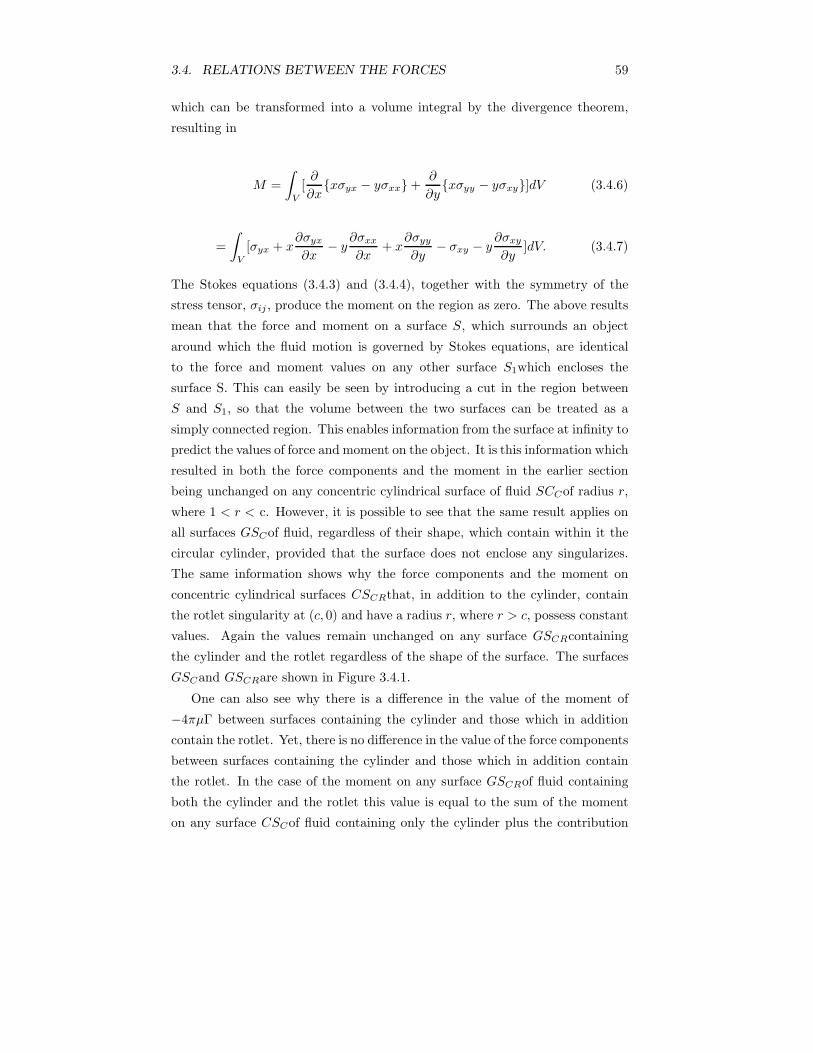
3.4. RELATIONS BETWEEN THE FORCES 59
which can be transformed into a volume integral by the divergence theorem,
resulting in
M =∫
V
[∂
∂x{xσyx − yσxx} +
∂
∂y{xσyy − yσxy}]dV (3.4.6)
=∫
V
[σyx + x∂σyx
∂x− y
∂σxx
∂x+ x
∂σyy
∂y− σxy − y
∂σxy
∂y]dV. (3.4.7)
The Stokes equations (3.4.3) and (3.4.4), together with the symmetry of the
stress tensor, σij , produce the moment on the region as zero. The above results
mean that the force and moment on a surface S, which surrounds an object
around which the fluid motion is governed by Stokes equations, are identical
to the force and moment values on any other surface S1which encloses the
surface S. This can easily be seen by introducing a cut in the region between
S and S1, so that the volume between the two surfaces can be treated as a
simply connected region. This enables information from the surface at infinity to
predict the values of force and moment on the object. It is this information which
resulted in both the force components and the moment in the earlier section
being unchanged on any concentric cylindrical surface of fluid SCCof radius r,
where 1 < r < c. However, it is possible to see that the same result applies on
all surfaces GSCof fluid, regardless of their shape, which contain within it the
circular cylinder, provided that the surface does not enclose any singularizes.
The same information shows why the force components and the moment on
concentric cylindrical surfaces CSCRthat, in addition to the cylinder, contain
the rotlet singularity at (c, 0) and have a radius r, where r > c, possess constant
values. Again the values remain unchanged on any surface GSCRcontaining
the cylinder and the rotlet regardless of the shape of the surface. The surfaces
GSCand GSCRare shown in Figure 3.4.1.
One can also see why there is a difference in the value of the moment of
−4πμΓ between surfaces containing the cylinder and those which in addition
contain the rotlet. Yet, there is no difference in the value of the force components
between surfaces containing the cylinder and those which in addition contain
the rotlet. In the case of the moment on any surface GSCRof fluid containing
both the cylinder and the rotlet this value is equal to the sum of the moment
on any surface CSCof fluid containing only the cylinder plus the contribution
60 CHAPTER 3. ANALYTICAL SOLUTION
Figure 3.4.1: Generalized surfaces. GSc and GSCRrepresent general surfaces
enclosing the circular cylinder and both the circular cylinder and the rotlet
respectively.
from the moment on the rotlet. As the stream function near the rotlet can be
expressed as
ψ ≈ ln(R1), (3.4.8)
which is equivalent to a ln(r) term in F0(r) in the expansion of the stream
function given by expression (3.3.1), the contribution to the moment from the
rotlet is −4πμΓ. Hence, the zero contribution on the inner surfaceGSCcombined
with that from the rotlet produces the result for the moment established earlier
on the outer surface GSCR. In a similar manner the force components between
the two surfaces can be related. However, the form of the stream function near
the rotlet, given by expression (3.4.8), results in there being no force in either
3.5. FLOWS AT INFINITY 61
direction on the rotlet. This results in the force components on the two surfaces
GSCand GSCRremaining the same. Hence, since they are both zero on the inner
surface, they are both zero on the outer surface. This means that provided one
knows the expansion of the stream function for flow around a body at large
values of r, and the expansion close to any singularity, it is possible using the
coefficients of FB1and GB1to determine the components of force acting both
on a surface of fluid containing the object at infinity and on the surface around
the singularity. The difference in these quantities will produce the force on the
body. In a similar manner the moment on the body can be produced from
the difference between the moment on the surface of fluid at large values of r
which contains the body and the moment on the singularity. In this case, the
two moments are obtained directly from the values of the coefficients of C0in
the appropriate regions, and their difference produces the moment on the body
itself.
3.5 Flows at Infinity
It has been establish earlier how the expansion of the stream function may be
used to predict the force and the moment acting on the circular cylinder. The
reverse situation will now be discussed, that is given a force and a moment acting
on a circular cylinder in the presence of a rotlet, what is the stream function
and how does this behave at large values of r?
In order to have a prescribed force −4πμΓ(A,−B)a−1, together with a mo-
ment −4πμΓC, acting on the circular cylinder it is necessary for the expansion
at large values of r to include the C0 ln(r), FB1rln(r) sin ϑ and GB1rln(r) cos ϑ
terms. Obviously as these terms are solutions of the biharmonic equation and
satisfy the boundary condition that the normal velocity on the cylinder is zero,
the linearity of the problem allows them to be combined with the earlier result
given by applying the boundary conditions in expression (3.1.3). All that re-
mains is to combine this result with another solution of the biharmonic equation
which satisfies the zero normal boundary condition but has a non zero tangential
velocity. The obvious choice of this additional solution is the uniform stream
potential flow solution past such a circular cylinder in order to balance the
FB1rln(r) sinϑ and FB1rln(r) cos ϑ terms, together with a rigid body rotation
arising from an (r2 − 1) term. The correct combination of the above extra solu-
62 CHAPTER 3. ANALYTICAL SOLUTION
tions will produce the required zero tangential velocity boundary condition on
r = 1. Hence, the complete additional solution is
C0[ln(r) − 12(r2 − 1)] + FB1[rln(r) − 1
2(r − r−1)] sinϑ
+GB1[rln(r) − 12(r − r−1)] cosϑ
(3.5.1)
and in order to produce the prescribed force it will be necessary for
FB1 = A, GB1 = B, (3.5.2)
and C0 = C + 1. (3.5.3)
The moment on a surface GSCR surrounding the circular cylinder and the rotlet
will have a moment −4πμΓ(C+1). When the value of the moment on the rotlet
−4πμΓ is subtracted for this value, it will produce the required value of −4πμΓC
on the circular cylinder itself. Hence, the required stream function is
ψ = ln(R1) − ln(R2c) + ln(r) +(r2 − 1)(rc cos ϑ− 1)
R22c
2
+ C[ln(r) − 12(r2 − 1)] +A[rln(r) − 1
2(r − r−1)] sinϑ
−B[rln(r) − 12(r − r−1)] cosϑ,
(3.5.4)
together with a vorticity value given by
ω =4c[r cosϑR2
2
− 2r(rc cos ϑ− 1)(rc− cosϑ)c2R4
2
+(rc cos ϑ− 1)
cR22
]
− 2C +2(A sinϑ−B cosϑ)
r.
(3.5.5)
The expression (3.5.4), with A = B = 0, corresponds to the result obtained
by Avudainayagam and Jothiram (1987) for eccentric rotational flow around a
circular cylinder in the presence of a rotlet singularity. The form of the above
stream function at large values of r will be
ψ ≈− 12Cr2 +Arln(r) sin ϑ−Brln(r) cos ϑ− 1
2Arsinϑ
+12(2c−B)rcosϑ+ (C + 1) ln(r).
(3.5.6)
3.5. FLOWS AT INFINITY 63
In the special situation when there is no force or moment on the circular cylinder
then
A = B = C = 0 (3.5.7)
and at large values of r the above form of the stream function reduces to
ψ ≈ 1crcosϑ+ ln(r) +
1c2
cos(2ϑ) − ln(c) +O(r−1). (3.5.8)
In fact the O(r−1) term is ( 1c3 cos(3ϑ)). If ln(R1) is retained in the expan-
sion (3.5.8) rather than ln(r) then the O(r−1) term is ( 1c3 cos(3ϑ)+ ccos(ϑ)).
Physically expression (3.5.8) represents at large distances from the cylinder,
a uniform stream of non-dimensional magnitude 1c flowing towards the origin
from the direction of the negative y axis, together with the effects of a rotlet of
non-dimensional strength unity at the origin. Hence, one has the situation first
established by Dorrepaal, O’Neill and Ranger (1984), namely, that provided a
rotlet is added at the correct position to the problem of a uniform flow past a
circular cylinder, its strength dependent on its distance from the origin and the
magnitude of the uniform stream, then what originally is an ill posed Stokes
problem becomes well posed. If ” * ” is used to denote dimensional quantities,
then expression (3.5.8) for the dimensional stream function becomes
ψ∗ ≈ Γ[1c∗r∗ cosϑ+ ln(r∗/a) +
a2
c∗2 cos(2ϑ) − ln(c∗/a) +O(r∗−1
), (3.5.9)
where c = c∗/a, so the dimensional position of the rotlet is (c∗, 0). The substi-
tution of expressions (3.5.4) and (3.5.5) into expressions (3.2.13), (3.2.14) and
(3.2.15), together with the evaluations of the resulting integrals using Simpson’s
rule, confirmed the values of A,B and C used to produce the analytical results.
It possible should show the force components and moments arising by Simpsons
rule corresponding to some values of A, B and C for which forces and moments
are known.
Numerical values of the integrals in expressions (3.2.13), (3.2.14) and (3.2.15)
were evaluated by Simpson’s rule for the non-dimensional stream function and
vorticity given by expressions (3.1.5) and (3.1.15) respectively. The procedure
was repeated with the non-dimensional steam function and vorticity represented
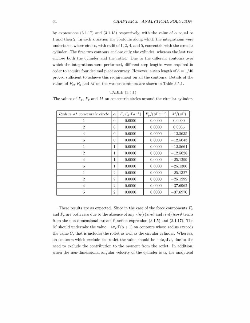
64 CHAPTER 3. ANALYTICAL SOLUTION
by expressions (3.1.17) and (3.1.15) respectively, with the value of α equal to
1 and then 2. In each situation the contours along which the integrations were
undertaken where circles, with radii of 1, 2, 4, and 5, concentric with the circular
cylinder. The first two contours enclose only the cylinder, whereas the last two
enclose both the cylinder and the rotlet. Due to the different contours over
which the integrations were performed, different step lengths were required in
order to acquire four decimal place accuracy. However, a step length of h = 1/40
proved sufficient to achieve this requirement on all the contours. Details of the
values of Fx, Fy and M on the various contours are shown in Table 3.5.1.
TABLE (3.5.1)
The values of Fx, Fy and M on concentric circles around the circular cylinder.
Radius of concentric circle α Fx/(μΓa−1) Fy/(μΓa−1) M/(μΓ)
1 0 0.0000 0.0000 0.0000
2 0 0.0000 0.0000 0.0035
4 0 0.0000 0.0000 −12.5635
5 0 0.0000 0.0000 −12.5643
1 1 0.0000 0.0000 −12.5664
2 1 0.0000 0.0000 −12.5628
4 1 0.0000 0.0000 −25.1299
5 1 0.0000 0.0000 −25.1306
1 2 0.0000 0.0000 −25.1327
2 2 0.0000 0.0000 −25.1292
4 2 0.0000 0.0000 −37.6962
5 2 0.0000 0.0000 −37.6970
These results are as expected. Since in the case of the force components Fx
and Fy are both zero due to the absence of any rln(r)sinϑ and rln(r)cosϑ terms
from the non-dimensional stream function expression (3.1.5) and (3.1.17). The
M should undertake the value −4πμΓ(α+ 1) on contours whose radius exceeds
the value C, that is includes the rotlet as well as the circular cylinder. Whereas,
on contours which exclude the rotlet the value should be −4πμΓα, due to the
need to exclude the contribution to the moment from the rotlet. In addition,
when the non-dimensional angular velocity of the cylinder is α, the analytical
3.6. CONCLUSIONS 65
form of the non-dimensional stream function results in the asymptotic expansion
at large values of r containing an (α+1)ln(r) term. The above numerical values
confirm the theoretical result that the moment on the circular cylinder is −4πμΓ
times the coefficient of the ln(r) term in the asymptotic expansion, provided any
contributions from singularities are excluded.
3.6 Conclusions
The Fourier Series Method has been used successfully to obtain an analytical
solution for the solution of the biharmonic equation outside a circular cylinder
with a rotelt placed in the solution domain.

Chapter 4
FLOW GENERATED BY
A ROTLET
4.1 Introduction
Before embarking on the numerical scheme which has been adopted to solve the
most general situation, namely when both the force and the moment on the
circular cylinder are non zero, a brief discussion of an alternate approach used
for the solution of the problem in the absence of any force or moment on the
circular cylinder, as yet unpublished, will be given. Hence, for the present, the
discussion relates to the well posed Stokes problem of a uniform stream flowing
past a circular cylinder in the presence of a rotlet, but in the absence of any
force or moment on the cylinder. By outlining the reason for the failure of this
numerical approach to accommodate the situation when the force and moment
on the cylinder are non zero leads one to understand why the later particular
numerical method has been chosen.
This alternative approach follows directly the technique presented by Tang
(1990) for the problem of uniform flow past a rotating circular cylinder at low
Reynolds number. In their paper the stream function was expressed as that
due to a uniform stream plus a perturbation affect which arises solely from the
presence of the rotating cylinder. It was assumed that this removal from the
stream function of the contribution due to the uniform stream would result in
the stream function perturbation being O(r) at large values of r. Expressing
67
68 CHAPTER 4. FLOW GENERATED BY A ROTLET
the perturbation stream function as some function of r and ϑ, namely f(r, ϑ),
multiplied by r, meant that f(r, ϑ) tended to zero as r → ∞. Inversion of
the radial coordinate resulted in the conditions at infinity being mapped to the
origin. Hence, the solution domain became 0 ≤ ϑ ≤ 2π and 0 ≤ ξ ≤ 1, where
ξ = r−1. In addition, the ϑ coordinate was scaled by defining η = (2ϑ)/π,
resulting in the final solution domain being 0 ≤ ξ ≤ 1 and 0 ≤ η ≤ 4. Although
this extra scaling was mainly for convenience and not a necessary part of the
method. Hence, the resulting governing partial differential equations for the
function f(ξ, η) and the vorticity ω had to be solved subject to both these
quantities being (i) zero on ξ = 0, (ii) taking the same values on η = 0 and
η = 4 in order to produce single value expressions, and (iii) on ξ = 1 that in the
original coordinates and variables corresponded to the no slip and zero normal
velocity conditions on the surface of the circular cylinder.
In applying this technique to the problem of uniform flow past a circular
cylinder in the presence of a rotlet the only modification required is the removal
of the singularity due to the rotlet, as well as the uniform stream, from the
expression for the stream function expression. Hence, in this situation the per-
turbation solution was again solely due to a circular cylinder, with the basic
flow being that of a uniform stream containing a rotlet. However, the difficulty
experienced was having placed a rotlet at the non-dimensional position (c, 0),
then in which direction should the uniform stream flow and what should be its
magnitude? Initially it was assumed that the non-dimensional stream function
for the uniform stream should have the form
ψ = λ1rcosϑ, (4.1.1)
that is it flows along the y-axis rather than along a general direction which
would have been indicated by choosing
ψ = λ1rcosϑ+ λ2rsinϑ. (4.1.2)
However, although expression (4.1.1) has, to a certain extent, introduced infor-
mation from the asymptotic solution by the knowledge of the direction of the
stream, it does no more than that since the magnitude of the stream required to
produce a well posed problem is still unknown. This conveyance of information
4.1. INTRODUCTION 69
can be readily seen if one compares expression (3.5.8) with expression (4.1.1).
Obviously this unknown value of λ1 prevents any direct solution.
An alternative approach to determining the direction of the stream could
have been the physical argument. This implies that the velocity at (r, ϑ), given
by (vr, vϑ) = (a, b), is related to that at (r,−ϑ), where (vr, vϑ) = (−a, b). Hence,
the velocity components in terms of the stream function, as shown in expression
(3.1.16), requires that the stream function is even in ϑ. This in turn requires
that the stream function is devoid of terms containing sin(nϑ).
The actual approach followed to overcome the unknown magnitude of the
stream was the realization that having expressed the form of the solution at
large values of r as
ψ ≈ λ1rcosϑ+ ln(R1), (4.1.3)
where the coefficient of ln(R1) was identical to the non-dimensional strength of
the rotlet at (c, 0), then the force and moment on the circular cylinder would
be zero. However, only when λ1 is a particular value, in this case c−1, will the
problem be well posed and produce these values for the force and moment. For
all other values of λ1 one will have Fx, Fy and M dependent on this parameter.
This means one can think of these three quantities as functions of λ1, and
only when λ1 possesses the correct value will all these quantities acquire their
necessary values. Hence, the technique adopted was that of a Newton Raphson
iteration on Fx(λ1). Prior to this the governing partial differential equations
were expressed in finite difference form and then solved for two values of λ1,
say λ1 = α and λ1 = β. The resulting two non zero values of Fx(λ1 = α)
and Fx(λ1 = β) being the values used in the Newton Raphson method in order
to establish a new value of λ1, say λ1 = γ, at which Fx(λ1) is zero. The finite
difference equations are resolved for this new value of λ1, and the resulting value
of Fx(λ1 = γ) used together with either Fx(λ1 = α), or Fx(λ1 = β), whichever
is closest to zero, to produce from the Newton Raphson solution a new value
of λ1. The process is continued until the value of Fx(λ1) reaches zero to within
the required tolerance. The value of λ1 obtained automatically resulted in the
correct values for Fy and M. This procedure could equally well have been applied
to setting either the value of Fy(λ1) or M(λ1) to zero.
However, what would have happened had one allowed the form of the stream
70 CHAPTER 4. FLOW GENERATED BY A ROTLET
function at large values of r due to the uniform stream to be more general,
namely that given by expression (4.1.3), so that neither the magnitude nor the
direction of the stream is known?. Hence, the problem is only well posed for
the special case of λ1 = c−1 and λ2 = 0. This in turn means that Fx, Fy
and M are functions of the parameters λ1 and λ2 and it is necessary to apply
Newton Raphson iteration on both these quantities for the two independent
parameters in order to produce Fx(λ1, λ2) = Fy(λ1, λ2) = 0. Again the value of
M acquires its required value. It should be emphasized that the ln(R1) term,
with coefficient unity, in the stream function at large values of r also conveys
a certain knowledge from the analytical solution into the numerical approach.
Since this term behaves like ln(r) at large values of r, so that its coefficient is
identical to the non-dimensional strength of the rotlet at (c, 0), it is implied
from the analytical solution that there is no moment on the cylinder.
It is possible to generalize the form of the solution at large values of r to
ψ ≈ λ1rcosϑ+ λ2rsinϑ+ λ3 ln(r) + ln(R1), (4.1.4)
in which case it is possible to iterate on the three expressions for Fx, Fy and M ,
which are now functions of the three parameters λ1, λ2 and λ3, until the zero
values for Fx, Fy and M are reached. In this situation the three parameters
acquire the values
λ1 = c−1, λ2 = 0, λ3 = 0. (4.1.5)
If, however, one wishes to introduce a non zero force on the cylinder, say F = F ∗x ,
then it is necessary to amend the expression for the stream function at large
values of r to the form
ψ ≈ λ1rcosϑ+ λ2rsinϑ+ λ4rlr(r) sin ϑ+ ln(R1). (4.1.6)
Similarly, for Fy = F ∗y , then
ψ ≈ λ1rcosϑ+ λ2rsinϑ+ λ5rlr(r) cos ϑ+ ln(R1). (4.1.7)
In both these instances the ln(R1) has continued to introduce some of the in-
formation derived from the asymptotic solution by way of the fact that its
4.1. INTRODUCTION 71
coefficient remains unity. Since the ln(R1) term at large values of r is identical
to the ln(r) in expression (3.5.8) which implies such a choice has introduced a
constraint that there is no moment on the cylinder. Again the Newton Raphson
iteration procedure was applied, but this time the quantities being iterated on
were (Fx − F ∗x ), Fy and M , or Fx, (Fy − F ∗
y ) and M.
However, once one moves to the situation when the moment is a non zero
quantity, regardless of whether the force remains so or not, then it is necessary
to have an expression for the stream function of the form
ψ ≈ λ1rcosϑ+ λ2rsinϑ+ λ3 ln(r) + λ6r2 + ln(R1). (4.1.8)
If in addition the components of force are also non zero, then one needs an
expression
ψ ≈ λ1rcosϑ+ λ2rsinϑ+ λ3 ln(r) + λ4rlr(r) cos ϑ+ λ5rlr(r) sin ϑ+ λ6r2 + ln(R1).
(4.1.9)
For the situation given by expression (4.1.8) and by expression (4.1.9) the num-
ber of unknown parameters exceeds the three dependent variables that are to
be prescribed, namely the two force components and the moment. Hence, the
previous approach fails since there is no longer any obvious extra quantities,
such as the value of the force and moment, that can be introduced.
The above approach has utilized the values of the force and moment, and as
these are quantities that naturally arise from the values of ψ and ω, and their
higher derivatives, around the circular cylinder it seems appropriate to switch to
an approach where such boundary quantities play the major role in the solution.
Hence, the numerical approach to be adopted in solving the general problem, as
well as the more restricted situations, is that of the Boundary Element Method.
Before discussing the Boundary Element Method in detail it should be
stressed that the method requires that the stream function and the vorticity
be expressed as a combination of two parts, where one part contains the terms
that tend to zero as r → ∞. Hence, the stream function is expressed as
ψ = λ1rcosϑ+ λ2rsinϑ+ λ3 ln(r) + λ4rlr(r) cos ϑ+ λ5rlr(r) sin ϑ
+ λ6r2 + λ7 + λ8 sin(2ϑ) + λ9 cos(2ϑ) + ln(R1) + ψ∗,
(4.1.10)
72 CHAPTER 4. FLOW GENERATED BY A ROTLET
where ψ∗ → 0 as r → ∞. The additional terms of O(1), namely
λ7 + λ8 sin(2ϑ) + λ9 cos(2ϑ), (4.1.11)
arise from the expressions (3.3.2), (3.3.5) and (3.3.6). Hence,
λ7 = D0, λ8 = FC2 and λ9 = GC2. (4.1.12)
It is possible to include the additional term λ8(r2 ln(r)−r2) in expression (4.1.10)
but if this is the case then the condition on the single valuedness of the pressure
must be included in the numerical procedure in order to ensure that λ8 becomes
zero. This was discussed in detail in the earlier section on the analytical solution.
In the case when there is neither a force nor a moment acting upon the
cylinder then it is possible from a physical argument to set
λ2 = λ5 = λ8 = 0. (4.1.13)
However, this restriction will not be imposed as the method is required to ac-
commodate (i) non zero force and moment and in the future (ii) flows involving
multi-bodies for which a physical argument will no longer be possible.
4.2 The Boundary Element Method (BEM)
The BEM has become an accepted and powerful method for the numerical so-
lution of a range of problems such as the diffusion of heat, some types of the
fluid flow motion, flows in porous media, viscous flow with the Reynolds num-
ber assumed to be zero, electrostatics and many others in which the governing
equations are the classical Laplace or biharmonic equation. The BEM consists
of the transformation of the partial differential equations into integral equations
relating only boundary values followed by the determination of the solution of
these integral equations. If the values at interior points are required, then they
may be calculated from the boundary data. Since all the numerical approxima-
tions occur on the boundaries, the dimensionality of the problem is reduced by
one and a smaller system of equations is obtained compared with those achieved
by differential methods.
4.2. THE BOUNDARY ELEMENT METHOD (BEM) 73
Over the past decades, numerous books and papers addressing the appli-
cations of the BEM to various problems, see for example Jaswon and Symm
(1976), Banerjee and Butterfield (1981), Brebbia et al (1984), Manzoor (1984)
and Kelmanson (1984), Brebbia and Gipson (1991), etc have been published.
As such it is now unnecessary to discuss fully the basic theory of the BEM.
The present section is concerned with the application of the BEM for the nu-
merical solution of a viscous steady flow problem at zero Reynolds number (the
biharmonic equation).
The crucial step in the application of the BEM is the transformation from
the differential equations to the integral equations. This is achieved by using
the divergence theorem
∫∂Ω
A · nds =∫
Ω
divAds, (4.2.1)
where A is a smooth vector function, which is second-order continuously
differentiable, defined within a domain Ω which is bounded by the closed contour
∂Ω, n is the outward normal to the domain, ds denotes the length element on
∂Ω and dS denote the surface element in Ω. The sense of the integration around
∂Ω is such that the domain is on the left as ∂Ω is traversed in the positive sense.
In order to be able to show how the integral identity (4.2.1) can be used
to transform differential equations into integral equations consider the Laplace
equation within a region Ω,
∇2ω(x, y) = 0, (x, y) ∈ Ω. (4.2.2)
Applying the divergence theorem to the vector function A = ω gradτ , where τ
is any smooth function defined within Ω, one obtains
∫∂Ω
(ωgradτ) · nds =∫
Ω
div(ωgradτ)dS, (4.2.3)
but gradτ · n = ∂τ/∂n, therefore
∫∂Ω
ω∂τ
∂nds =
∫Ω
(gradω · gradτ + ω∇2τ)dS, (4.2.4)
74 CHAPTER 4. FLOW GENERATED BY A ROTLET
Similarly, applying the divergence theorem to the vector function τ gradω gives
∫∂Ω
τ∂ω
∂nds =
∫Ω
(gradτ · gradω + τ∇2ω)dS, (4.2.5)
Subtracting equation (4.2.5) from equation (4.2.4) one obtains∫∂Ω
(ω∂τ
∂n− τ
∂ω
∂n)ds =
∫Ω
(ω∇2τ − τ∇2ω)dS. (4.2.6)
This identity is known as Green’s Theorem and it holds for any smooth functions
ω and τ defined within a plane domain Ω which is bounded by a closed contour
∂Ω.
Using the fact that ∇2ω = 0 in Ω, equation (4.2.6) becomes
∫∂Ω
(ω∂τ
∂n− τ
∂ω
∂n)ds =
∫Ω
ω∇2τdS. (4.2.7)
Furthermore, taking τ to be a particular solution of the Poisson equation
∇2τ(p, q) = δ(p− p0), (4.2.8)
where p = (x, y) and p0 = (x0, y0) are in Ω and δ is the Dirac delta function.
Then equation (4.2.7) becomes
η(p)ω(p) =∫
∂Ω
ω(q)∂τ(p, q)∂n
ds−∫
∂Ω
∂ω(q)∂n
τ(p, q)dS, (4.2.9)
where p ∈ Ω ∪ ∂Ω, q ∈ ∂Ω and η(p) is a constant dependent upon the location
of the point p and is given by
η(p) = η(p) =
⎧⎪⎪⎪⎪⎪⎪⎨⎪⎪⎪⎪⎪⎪⎩
2π when p ∈ Ω
θ when p ∈ ∂Ω, θ is the angle between
the tangents to∂Ω on either side of p
0 when p /∈ Ω ∪ ∂Ω.
(4.2.10)
This boundary integral equation is usually refer
| p− p0 |= {(x− x0)2 + (y − y0)2}1/2. (4.2.11)
4.2. THE BOUNDARY ELEMENT METHOD (BEM) 75
Taking the prime (′) to denote the derivative in the direction of the outward
normal to ∂Ω, and the boundary value of ω(p) as φ(p), then the integral equation
(4.2.9) becomes
∫∂Ω
φ(q) ln′ | p− q | dq −∫
∂Ω
φ′(q) ln | p− q | dq = η(p)ω(p). (4.2.12)
Using the equation (4.2.12), the ω can be determined at any point Ω∪ ∂Ω pro-
vided φ and ∂φ/∂n are known at all points on the boundary ∂Ω. Unfortunately,
in most of the physical problems φ and ∂φ/∂n are not simultaneously prescribed
at all such points. However, it is still possible to apply Green’s Integral Formula.
In equation (4.2.12) taking p, q ∈ ∂Ω one has
∫∂Ω
φ(q) ln′ | p− q | dq −∫
∂Ω
φ′(q) ln | p− q | dq = η(p)φ(p). (4.2.13)
If one knows either φ(p) or φ′(p) on ∂Ω one can obtain the other function by
using equation (4.2.13). Then substitution of both these values into equation
(4.2.12) gives the solution of the Laplace equation in Ω.
In practice analytical solutions of the integral equations (4.2.12) and (4.2.13)
are usually impossible and thus some form of numerical approximation is nec-
essary. This is achieved by first subdividing the boundary ∂Ω into N segments
∂Ωj , j = 1, 2, . . . ,N. On each segment φ and φ′ are approximated by constants
φj , and φ′j , where φj and φ′j take the values of φ and φ′ at the midpoint of
the segment ∂Ωj , respectively. Then the integral formula (4.2.12) and (4.2.13)
become
N∑j=1
φj
∫∂Ωj
ln′ | p− q | dq −N∑
j=1
φ′j
∫∂Ωj
ln | p− q | dq = η(p)ω(p), (4.2.14)
N∑j=1
φj
∫∂Ωj
ln′ | pi− q | dq − ηiφi −
N∑j=1
φ′j
∫∂Ωj
ln | pi− q | dq = 0,
i = 1, 2, . . .N.
(4.2.15)
where pi is the midpoint of the segment ∂Ωi and ηi = η(pi).
Using the expression (4.2.15) one obtains
76 CHAPTER 4. FLOW GENERATED BY A ROTLET
N∑j=1
φj(∫
∂Ωj
ln′ | pi− q | dq − ηiδij) −
N∑j=1
φ′j
∫∂Ωj
ln | pi− q | dq = 0,
i = 1, 2, . . .N.
(4.2.16)
If one writes
Gij =∫
∂Ωj
ln | pi− q | dq, (4.2.17)
and
Eij =∫
∂Ωj
ln′ | pi− q | dq − η(p
i)δij , (4.2.18)
where δij is Kronecker’s delta function. Then the equation (4.2.16) may be
written as follow
N∑j=1
Eijφj −N∑
j=1
Gijφ′j = 0. i = 1, 2, . . . , N. (4.2.19)
A more accurate approximation of the solution of the Laplace equation using
the BEM can be obtained by using a linear function to approximate φ and φ′
on each boundary segment. In this case one lets
φj = (1 − ξ)φ(qj−1
) + ξφ(qj), (4.2.20)
φ′j = (1 − ξ)φ′(qj−1
) + ξφ′(qj), (4.2.21)
where qj−1 and qj are the end points of ∂Ωj , ξ is a linear function which increases
from zero at qj−1
to unity at qj. Inserting these functions φj and φ′j into
equations (4.2.12) and (4.2.13) one obtains
N∑j=1
{φj−1
∫∂Ωj
(1 − ξ) ln′ | p− q | dq + φj
∫∂Ωj
ξ ln′ | p− q | dq}
−N∑
j=1
{φ′j−1
∫∂Ωj
(1 − ξ) ln | p− q | dq + φ′j
∫∂Ωj
ξ ln | p− q | dq}
= η(p)ω(p) p ∈ Ω̄ q ∈ ∂Ω
(4.2.22)
4.2. THE BOUNDARY ELEMENT METHOD (BEM) 77
N∑j=1
{φj−1
∫∂Ωj
(1 − ξ) ln′ | pi− q | dq + φj
∫∂Ωj
ξ ln′ | pi− q | dq}
−N∑
j=1
{φ′j−1
∫∂Ωj
(1 − ξ) ln | pi− q | dq + φ′j
∫∂Ωj
ξ ln | pi− q | dq}
= η(pi)φi, i = 1, 2, . . . , N p
i, q ∈ ∂Ω
(4.2.23)
where φj and φ′j denote φ(pj) and φ′(p
j), and φ0 = φN and φ′0 = φ′N respec-
tively. As with the classical BEM (4.2.19), the expression (4.2.23) reduces to a
linear system of algebraic equations of the form
N∑j=1
E∗ijφj −
N∑j=1
G∗ijφ
′j = 0, i = 1, 2, . . . , N (4.2.24)
where
E∗ij =
∫∂Ωj+1
(1 − ξ) ln′ | pi− q | dq +
∫∂Ωj
ξ ln′ | pi− q | dq − ηiδij , (4.2.25)
G∗ij =
∫∂Ωj+1
(1 − ξ) ln | pi− q | dq +
∫∂Ωj
ξ ln | pi− q | dq, (4.2.26)
∂ΩN+1 = ∂Ω1 and pi is the common point of the segments ∂Ωi and ∂Ωi+1.
If the segment ∂Ωj is a straight line, then the integrals occurring in the
equations (4.2.12), (4.2.13), (4.2.22) and (4.2.23) may be evaluated exactly to
obtain
∫∂Ωj
ln′ | p− q | dq = I1, (4.2.27)
∫∂Ωj
ln | p− q | dq = J1, (4.2.28)
∫∂Ωj
ξ ln′ | p− q | dq =1h
(a cosβI1 + I2), (4.2.29)
∫∂Ωj
ξ ln | p− q | dq =1h
(a cosβJ1 + J2), (4.2.30)
78 CHAPTER 4. FLOW GENERATED BY A ROTLET
with, see Manzoor (1984),
I1 = γ, (4.2.31)
I2 = asinβ(lnb− lna), (4.2.32)
J1 =acosβ(lna− lnb) + h(lnb− 1) + aγ sinβ, (4.2.33)
J2 =12(b2lnb− a2lna) − 1
4(b2 − a2), (4.2.34)
where qj−1 and qj are the endpoints of ∂Ωj , see figure 4.2.1, and a, b and h
are the lengths of the lines joining p to qj−1, p to qj and qj−1 to qj , respectively,
and β and γ are the angles qjqj−1p and qj−1pqj, respectively.
For steady two-dimensional flow of an incompressible Newtonian fluid the
Navier-Stokes and continuity equations reduce to
∇p = ∇2u, (4.2.35)
∇ · u = 0, (4.2.36)
when the Reynolds number is assumed to be very small. On introducing
the stream function, ψ say, such that ∂ψ/∂x = −vy and ∂ψ/∂y = vx, then ψ
satisfies the biharmonic equation, see Batchelor (1967),
∇4ψ = 0. (4.2.37)
On introducing the vorticity, ω, equation (4.2.37) may be written in the
form
∇2ψ = ω, (4.2.38)
∇2ω = 0. (4.2.39)
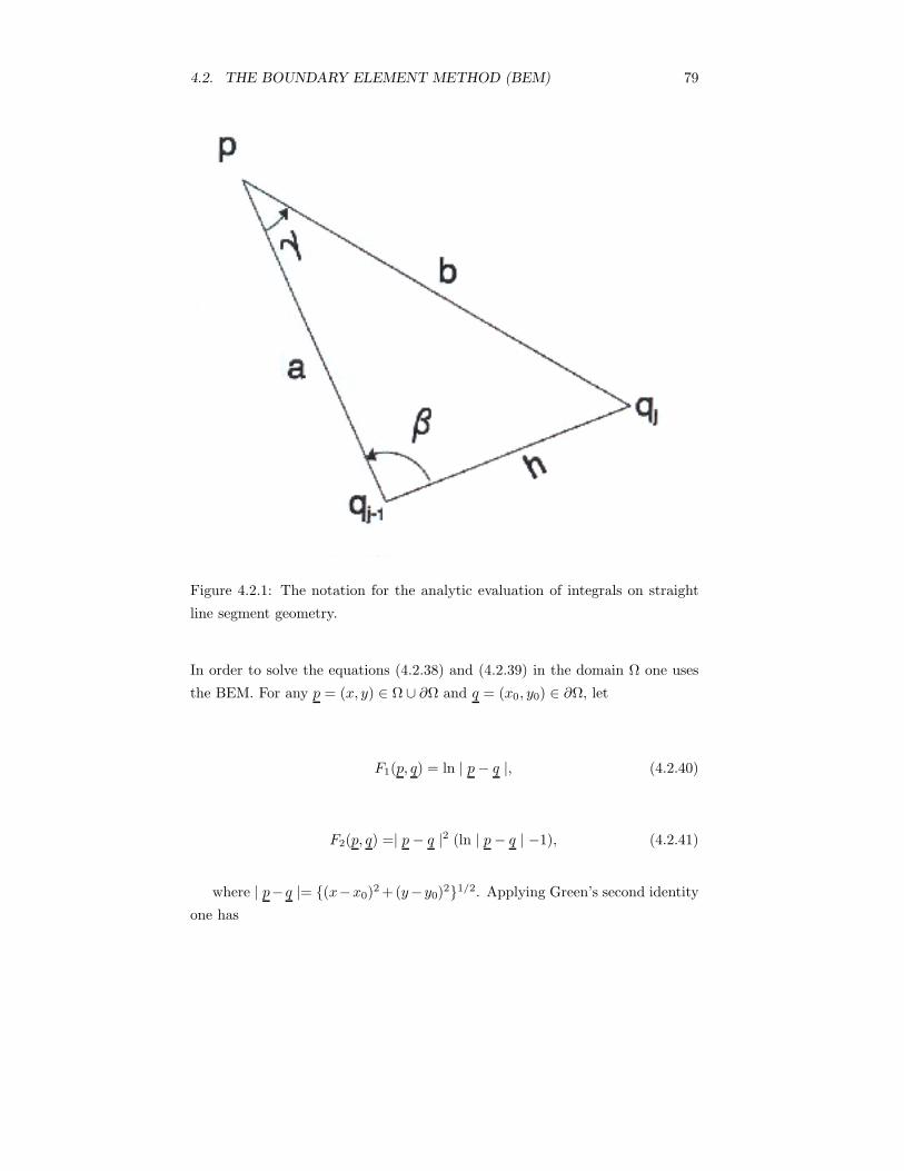
4.2. THE BOUNDARY ELEMENT METHOD (BEM) 79
Figure 4.2.1: The notation for the analytic evaluation of integrals on straight
line segment geometry.
In order to solve the equations (4.2.38) and (4.2.39) in the domain Ω one uses
the BEM. For any p = (x, y) ∈ Ω ∪ ∂Ω and q = (x0, y0) ∈ ∂Ω, let
F1(p, q) = ln | p− q |, (4.2.40)
F2(p, q) =| p− q |2 (ln | p− q | −1), (4.2.41)
where | p− q |= {(x−x0)2 +(y−y0)2}1/2. Applying Green’s second identity
one has
80 CHAPTER 4. FLOW GENERATED BY A ROTLET
η(p)ψ(p) =∫
∂Ω
ψ(q)F ′1(p, q)dq −
∫∂Ω
ψ′(q)F1(p, q)dq
14
∫∂Ω
ω(q)F ′2(p, q)dq −
14
∫∂Ω
ω′(q)F2(p, q)dq,(4.2.42)
η(p)ω(p) =∫
∂Ω
ω(q)F ′1(p, q)dq −
∫∂Ω
ω′(q)F1(p, q)dq. (4.2.43)
A similar strategy is now followed to that employed above when solving
the Laplace equation in order to produce a solution from the integral equations
(4.2.42) and (4.2.43). That is, the boundary is first subdivided into N segments,
∂Ωj , and the stream function, ψ, its derivative, ψ′, the vorticity, ω, and its
derivative, ω′, are approximated by piecewise constant functions. This results
in equation (4.2.42) producing the system of algebraic equations
N∑j=1
{Eijψj −Gijψ′j + Lijωj −Mijω
′j} = 0, i = 1, . . . , N (4.2.44)
where Gij and Eij are as given in equations (4.2.17) and (4.2.18) respectively,
and Lij and Mij are given by
Lij =14
∫∂Ω
ω(q)F ′2(p, q)dq, (4.2.45)
Mij =14
∫∂Ω
ω(q)F2(p, q)dq, (4.2.46)
Equation (4.2.44) represents N equations in 4N unknowns and a further
N equations are derived from equation (4.2.19). This produces the system of
algebraic equations
∑Nj=1 Eijψj −Gijψ
′j + Lijωj −Mijω
′j = 0∑N
j=1 Eijωj −Gijω′j = 0
}i = 1, . . . , N (4.2.47)
With the application of the appropriate boundary conditions the system of
equations (4.2.47) can be solved and equations (4.2.42) and (4.2.43) used to find
the value of the stream function, ψ, and the vorticity, ω, at any point within
the solution domain, Ω.
4.2. THE BOUNDARY ELEMENT METHOD (BEM) 81
In order to obtain a more accurate numerical solution linear elements may
be used. In this case the unknown functions ψ,ψ′, ω and ω′ are approximated
by linear functions on each boundary segment such that
ψj = (1 − ξ)ψ(qj−1
) + ξψ(qj), (4.2.48)
ψ′j = (1 − ξ)ψ′(q
j−1) + ξψ′(q
j), (4.2.49)
ωj = (1 − ξ)ω(qj−1
) + ξω(qj), (4.2.50)
ω′j = (1 − ξ)ω′(q
j−1) + ξω′(q
j), (4.2.51)
where ξ is as defined in equations (4.2.19) and (4.2.20). Inserting these
approximations into the integral equations (4.2.42) and (4.2.43) and rearranging
the resulting equations produces the following system of algebraic equations
∑Nj=1 E
∗ijψj −G∗
ijψ′j + L∗
ijωj −M∗ijω
′j = 0∑N
j=1 E∗ijωj −G∗
ijω′j = 0
}i = 1, . . . , N (4.2.52)
where E∗ij and G∗
ij are given in equations (4.2.25) and (4.2.26) respectively
and L∗ij and M∗
ij are given by
L∗ij =
14
N∑j=1
{∫
∂Ωj+1
(1 − ξ)F ′2(p, q)dq +
∫∂Ωj
ξF ′2(p, q)dq}, (4.2.53)
M∗ij =
14
N∑j=1
{∫
∂Ωj+1
(1 − ξ)F2(p, q)dq +∫
∂Ωj
ξF2(p, q)dq}. (4.2.54)
Similarly, if the segment ∂Ωj is a straight line, then the integrals occurring in
the equations (4.2.45), (4.2.46), (4.2.53) and (4.2.54) may be evaluated exactly
using the notation shown in figure 4.2.1, namely
∫∂Ωj
F ′2(p, q)dq = a(2J1 − h) sinβ, (4.2.55)
82 CHAPTER 4. FLOW GENERATED BY A ROTLET
∫∂Ωj
F2(p, q)dq =13(h− a cosβ)3(lnb− 4
3) +
13(a cosβ)3(lna− 4
3) +
(a sinβ)2(J1 −23h− 1
3aγ sinβ),
(4.2.56)
∫∂Ωj
ξF ′2(p, q)dq =
2ha sinβ(a cos βJ1 + J2) −
12ah sinβ,
(4.2.57)
∫∂Ωj
ξF2(p, q)dq =1ha cosβ
∫∂Ωj
F2(p, q)dq +
14h
(b4lnb− a4lna) − 516h
(b4 − a4)(4.2.58)
It should be stressed that throughout the present work the emphasis when
applying the Boundary Element Method has been on constant elements rather
linear elements.
4.3 The Numerical Solution
In applying the above method to the flow past a circular cylinder in the presence
of a rotlet the fluid domain Ω is the area outside the cylinder and the ∂Ω is the
contour of the cylinder. However, prior to using the method it is necessary to
accommodate the infinity boundary conditions. Since the BEM requires that
the non-dimensional stream function and vorticity used in equations (4.2.47)
are both O(r−1) at large values of r, it is necessary that these quantities are
expressed as perturbation values about their asymptotic expansions at large
values of r and the perturbation parts used in these equations. The number
of terms in the expansions being sufficient to ensure that both perturbation
quantities decay to zero to satisfy the above infinity conditions. Hence,
ψ = ψA + ψ∗, and ω = ωA + ω∗, (4.3.1)
where ψA and ωA are the asymptotic expansions of ψ and ω as r → ∞, and ψ∗
and ω∗ are the perturbations values about these expansions that tend to zero
as r → ∞, where
4.3. THE NUMERICAL SOLUTION 83
∇2ψA = ωA and ∇2ωA = 0. (4.3.2)
So the biharmonic equation for the stream function can be written as
∇2ψ∗ = (ωA −∇2ψA) + ω∗, (4.3.3)
∇2ω∗ = −∇2ωA. (4.3.4)
Using the equations in (4.3.2) reduces equations (4.3.3) and (4.3.4) to
∇2ψ∗ = ω∗, (4.3.5)
∇2ω∗ = 0. (4.3.6)
This results in the stream function and vorticity expressions in the above Bound-
ary Element Method being replaced by ψ∗ and ω∗. The original boundary con-
ditions on the cylinder, provided the cylinder is not rotating, are as given in
expression (3.1.3). However, the boundary conditions on ψ∗ and ω∗ will be as
follows,
ψ∗ = −ψA and∂ψ∗
∂r= −∂ψA
∂r, . . . on r = 1. (4.3.7)
Hence, in equations (4.2.47)ψ∗j and ψ′
j∗, which have been replaced ψj and
ψ′j , will now take the values −ψAj and −ψ′
Aj.
In expression (4.2.47) there are 2n equations in 4n unknowns. However,
if the values of ψ∗j and ψ′
j∗ are free of any unknowns then these will provide
another 2n conditions, so after their substitution one has a closed system of 2n
equations in 2n unknowns. Unfortunately, the expressions for ψ∗j and ψ′
j∗ will,
from expression (4.1.10), be given by
ψ∗j = −λ1 cos(θj) − λ2 sin(θj) − λ6 − λ7 − λ8 sin(2θj) − λ9 cos(2θj) − ln(R1(1)),
(4.3.8)
84 CHAPTER 4. FLOW GENERATED BY A ROTLET
ψ′j∗ = − λ1 cos(θj) − λ2 sin(θj) − λ3 − λ4 cos(θj)
− λ5 sin(θj) − 2λ6 −(1 − c cos(θj))
R21(1)
, j = 1, . . . , N,(4.3.9)
where R21(1) = (1 + c2 − 2c cos(ϑj)).
Case (a) uniform stream at infinity, so general situation has λ3 = λ4 = λ5 =
λ6 = 0.
Obviously the extra unknowns λj , where j = 1, . . . , 9, in the most general
situation of non-zero force and moment on the cylinder, will require extra con-
ditions. For the present the unknowns related to the non zero force and moment
on the cylinder, namely λ3, λ4, λ5 and λ6, will be set to zero. In addition, if the
direction of the stream is introduced by way of prescribing λ2 also to be zero,
then this results in there being an extra 4 unknowns, which require an extra 4
conditions. However, this extra restriction will not be imposed. It is proposed
to introduce the conditions that there should be no force or moment on the
cylinder, so expressions (3.2.13), (3.2.14) and (3.2.15) have ψ and ω replaced
by ψ∗ + ψA and ω∗ + ωA, respectively. The parts of the integrals involving
ψA and ωA are evaluated analytically, producing linear expressions in the un-
knowns λj .The other parts involving ψ∗ and ω∗ are expressed after numerical
integration by Simpson’s method as linear expressions of ψj , ψ′j∗, ω∗
j and ω′j∗.
Hence, the resulting expressions for the force and moment on the cylinder may
be written as
Fx = 0 = +∑(N−1)/2
j=1 [(ω′∗2j−1 + 4ω′∗
2j + ω′∗2j+1)
−(ω∗2j−1 + 4ω∗
2j + ω∗2j+1)](sin(θj)(2π/(3N)),
}(4.3.10)
Fy = 0 = −∑(N−1)/2
j=1 [(ω′∗2j−1 + 4ω′∗
2j + ω′∗2j+1)
−(ω∗2j−1 + 4ω∗
2j + ω∗2j+1)](cos(θj)(2π/(3N)),
}(4.3.11)
M = 0 = −(N−1)/2∑
j=1
[(ω′∗2j−1 + 4ω′∗
2j + ω′∗2j+1)](2π/(3N)), (4.3.12)
where ω∗1 = ω∗
N , ω′∗1 = ω′∗
N and ψ∗1 = ψ∗
N , ψ′∗1 = ψ′∗
N .
Hence, equations (4.2.47), together with equations (4.3.10), (4.3.11) and
(4.3.12), and the expressions (4.3.8) and (4.3.9) result in (2N + 3) equations in
terms of the (2N + 5) unknowns, namely ω∗j , ω
′∗j , j = 1, . . . .., N, λ1, λ2, λ7, λ8
4.3. THE NUMERICAL SOLUTION 85
and λ9. Obviously, two further equations are required to close the above system.
One of these arises from the fact that the pressure distribution must be single
valued. Hence, from the component of the Stokes equation in the ϑ direction,
namely
0 = −1r
∂p
∂θ+∂ω
∂θ, (4.3.13)
one obtains that
0 =∫ 2π
0
∂ω
∂θdθ. (4.3.14)
On applying Simpson’s rule to evaluate the integral one obtains
0 = −(N−1)/2∑
j=1
[(ω′∗2j−1 + 4ω′∗
2j + ω′∗2j+1)]. (4.3.15)
This results in equations (4.3.10), (4.3.11), (4.3.12) and (4.3.15) providing 4
of the necessary 5 extra equations that are required. In order to obtain the
other equation it is necessary to appeal to the form of ψ∗ at large values of r.
If in equation (4.2.42) p is taken as p(r1, ϑ1), where r1 is some large value of r,
then ψ∗(p(r1, ϑ1) is approximately zero. Unfortunately, from the expansion in
expression (4.1.10) and expression (4.3.1) this means that one has introduced
an error of O(r−11 ) into the solution. Hence, extremely large values of r1 are
required to generate accurate results, but this difficulty can be overcome to
some extent by adding the next term in the expansion into expression (4.1.10),
namely
(λ10 sinϑ+ λ11 cosϑ+ λ12 sin(3ϑ) + λ13 cos(3ϑ))1r. (4.3.16)
By introducing these extra terms into the expansion, the approximation of
ψ∗(p(r1, ϑ1) by zero results in an error of only O(r−21 ), and therefore a higher
degree of accuracy can be achieved without the need for such a large value of
r1. However, before one can obtain this solution it is necessary to find further
equations to balance the additional unknowns λ10, λ11, λ12 and λ13 that have
been introduced. The obvious means of achieving these is to take another 4
86 CHAPTER 4. FLOW GENERATED BY A ROTLET
values of p at large values of r, namely p(rj , ϑj) with rj > 10 for j = 2, 3, 4, 5
and apply equation (4.2.42) with ψ∗(p(rj , ϑj) = 0 for j = 2, 3, 4, 5.
Even with the extra terms in the equations the error that has been introduced
by setting ψ∗(p) in equation (4.2.42) to be zero is O(r−2), or O(r−1) without
the additional terms, where r is the smallest of the values of rj , j = 1, 2, 3, 4, 5.
The necessity for these extra terms can be avoided if instead of choosing point
p in expression (4.2.42) to be at some large value of r one takes it to be inside
the cylinder, namely p(rI1, ϑ1), where rI1 < 1. This means that η(p) vanishes
and there is no need to approximate ψ∗(p).
Case (b) Unbounded flow at infinity corresponding to a stokeslet at the
origin, so general situation has λ3 = λ6 = 0.
In this situation one has a specified non-dimensional force 4π(−A,B), and
the terms λ4rln(r) sinϑ and λ5rln(r) cos ϑ must now be retained in the asymp-
totic expansion (4.1.10) of ψ. Hence, equations (4.3.10) and (4.3.11) have to be
replaced by
Fx = −4πA = −4πλ5 +∑(N−1)/2
j=1 [(ω′∗2j−1 + 4ω′∗
2j + ω′∗2j+1)
−(ω∗2j−1 + 4ω∗
2j + ω∗2j+1)](sin(θj)(2π/(3N)),
}(4.3.17)
Fy = 4πB = 4πλ4 −∑(N−1)/2
j=1 [(ω′∗2j−1 + 4ω′∗
2j + ω′∗2j+1)
−(ω∗2j−1 + 4ω∗
2j + ω∗2j+1)](cos(θj)(2π/(3N)).
}(4.3.18)
However, the introduction of the extra unknowns λ4 and λ5 makes it neces-
sary to apply equation (4.2.42) three times with p as p(rIj , ϑj), where rIj < 1
for j = 1, 2, 3, with the corresponding η(p) being zero as the points are all within
the cylinder.
Case (c) Unbounded flow at infinity which is a combination of a uniform
stream and a rotational far field, so general situation has λ4 = λ5 = 0.
In this situation one has a prescribed non-dimensional moment, −4πC, hence
the need to retain the terms λ3 ln(r) and λ6r2 in the asymptotic expansion of ψ
given by expression (4.1.10). Equations (4.3.10) and (4.3.11) replace equations
(4.3.17) and (4.3.18). In addition, equation (4.3.12) is replaced by
M = −4πC = 8πλ6 −(N−1)/2∑
j=1
[(ω∗2j−1 + 4ω∗
2j + ω∗2j+1)](2π/(3N)). (4.3.19)
4.4. NUMERICAL RESULTS 87
Again the introduction of two additional constants, this time λ3 and λ6, require
the enforcement of equation (4.2.42) at three points within the cylinder.
Case (d) Combination of unbounded flows at infinity due to stokeslet at the
origin together with a rotational far field, so general situation has λj = 0, for
j = 1, . . . .., 9.
With both the force and the moment specified it is necessary to apply the
equations (4.3.17), (4.3.18) and (4.3.19). As with cases, (a), (b) and (c) the
single valued pressure condition, given by equation (4.3.15), remains one of the
extra equations. As now all the constants λj , j = 1, . . . . . . , 9, are present it is
necessary to enforce equation (4.2.42) at 5 points (rIj , ϑj) within the cylinder
instead of at just 3 points as in Cases (b) and (c).
It is possible to include the term A0(r2 ln(r) − r2) from expression (3.3.2),
which vanished due to the single valueness of the pressure, in the asymptotic
part of expression (4.1.10). However, on doing so, in the form λ0(r2 ln(r)−r2) to
conform with the adopted notation, it would require the modification of equation
(4.3.15), together with the implementation of equation (4.2.42) at another point
within the circular cylinder. Hence, increasing the number of points where this
equation has to be applied in the most general situation, namely Case (d), from
5 to 6. The actual condition that would replace equation (4.3.15) would be
0 = 8πλ0 −(N−1)/2∑
j=1
[(ω′∗2j−1 + 4ω′∗
2j + ω′∗2j+1)](2π/(3N)). (4.3.20)
The term in ψ which is just a multiple of ϑ will not be considered at any stage
since it obviously violates the periodicity and has been neglected throughout.
4.4 Numerical Results
In all the numerical calculations the rotlet has been located along the x-axis at
the non-dimensional distance c from the center of the cylinder and the value
of c has been taken to be 3 in order to correspond with the calculations by
Dorrepaal et al. (1984)
Figure 4.4.1 shows the streamlines relating to expression (3.1.5). The pattern
is identically to that presented by Dorrepaal et.al. (1984). Figures 4.4.2 and
4.4.3 show the corresponding streamline patterns when the cylinder rotates with
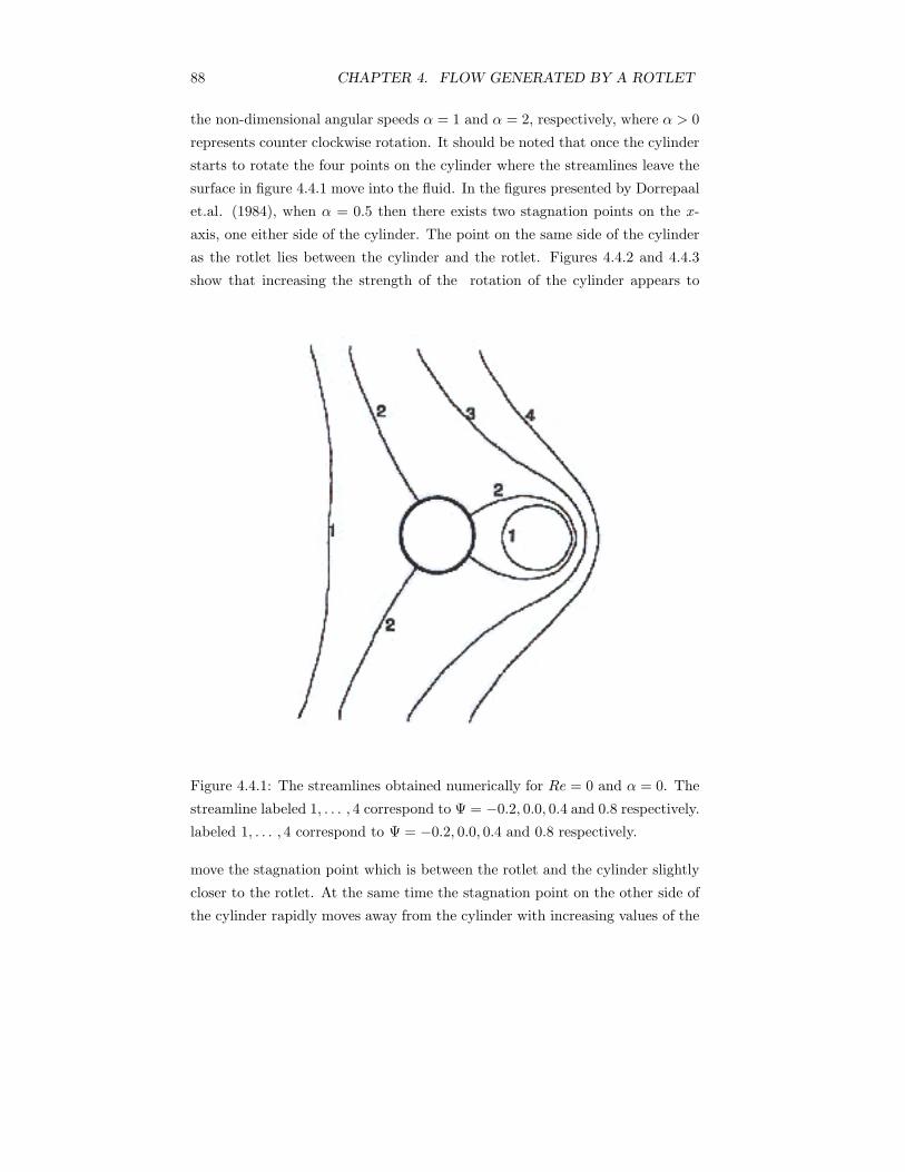
88 CHAPTER 4. FLOW GENERATED BY A ROTLET
the non-dimensional angular speeds α = 1 and α = 2, respectively, where α > 0
represents counter clockwise rotation. It should be noted that once the cylinder
starts to rotate the four points on the cylinder where the streamlines leave the
surface in figure 4.4.1 move into the fluid. In the figures presented by Dorrepaal
et.al. (1984), when α = 0.5 then there exists two stagnation points on the x-
axis, one either side of the cylinder. The point on the same side of the cylinder
as the rotlet lies between the cylinder and the rotlet. Figures 4.4.2 and 4.4.3
show that increasing the strength of the rotation of the cylinder appears to
Figure 4.4.1: The streamlines obtained numerically for Re = 0 and α = 0. The
streamline labeled 1, . . . , 4 correspond to Ψ = −0.2, 0.0, 0.4 and 0.8 respectively.
labeled 1, . . . , 4 correspond to Ψ = −0.2, 0.0, 0.4 and 0.8 respectively.
move the stagnation point which is between the rotlet and the cylinder slightly
closer to the rotlet. At the same time the stagnation point on the other side of
the cylinder rapidly moves away from the cylinder with increasing values of the
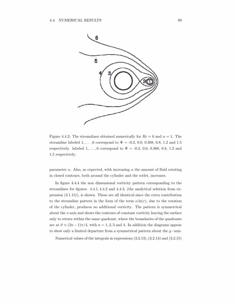
4.4. NUMERICAL RESULTS 89
Figure 4.4.2: The streamlines obtained numerically for Re = 0 and α = 1. The
streamline labeled 1, . . . ,6 correspond to Ψ = -0.2, 0.0, 0.388, 0.8, 1.2 and 1.5
respectively. labeled 1, . . . , 6 correspond to Ψ = -0.2, 0.0, 0.388, 0.8, 1.2 and
1.5 respectively.
parameter α. Also, as expected, with increasing α the amount of fluid rotating
in closed contours, both around the cylinder and the rotlet, increases.
In figure 4.4.4 the non dimensional vorticity pattern corresponding to the
streamlines for figures. 4.4.1, 4.4.2 and 4.4.3, (the analytical solution from ex-
pression (3.1.15)), is shown. These are all identical since the extra contribution
to the streamline pattern in the form of the term α ln(r), due to the rotation
of the cylinder, produces no additional vorticity. The pattern is symmetrical
about the x-axis and shows the contours of constant vorticity leaving the surface
only to return within the same quadrant, where the boundaries of the quadrants
are at ϑ � (2n− 1)π/4, with n = 1, 2, 3 and 4. In addition the diagrams appear
to show only a limited departure from a symmetrical pattern about the y−axis.
Numerical values of the integrals in expressions (3.2.13), (3.2.14) and (3.2.15)
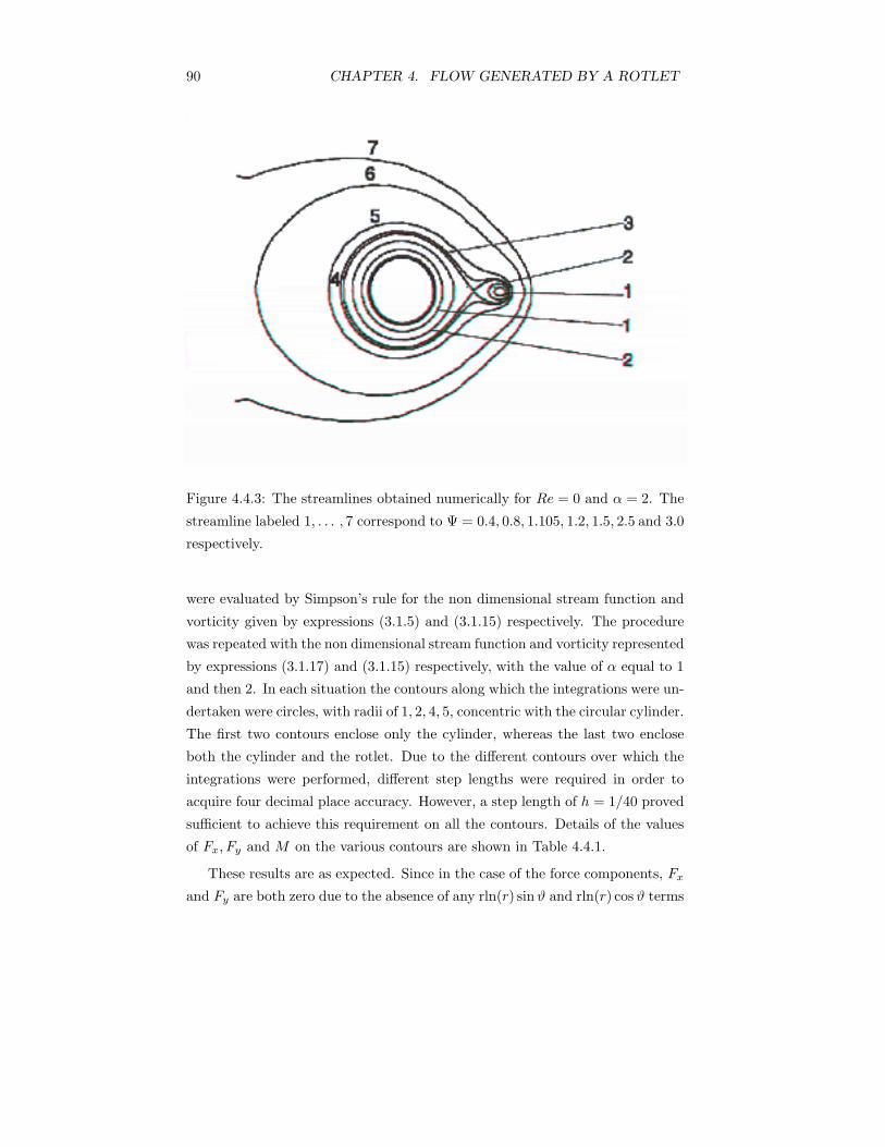
90 CHAPTER 4. FLOW GENERATED BY A ROTLET
Figure 4.4.3: The streamlines obtained numerically for Re = 0 and α = 2. The
streamline labeled 1, . . . , 7 correspond to Ψ = 0.4, 0.8, 1.105, 1.2, 1.5, 2.5 and 3.0
respectively.
were evaluated by Simpson’s rule for the non dimensional stream function and
vorticity given by expressions (3.1.5) and (3.1.15) respectively. The procedure
was repeated with the non dimensional stream function and vorticity represented
by expressions (3.1.17) and (3.1.15) respectively, with the value of α equal to 1
and then 2. In each situation the contours along which the integrations were un-
dertaken were circles, with radii of 1, 2, 4, 5, concentric with the circular cylinder.
The first two contours enclose only the cylinder, whereas the last two enclose
both the cylinder and the rotlet. Due to the different contours over which the
integrations were performed, different step lengths were required in order to
acquire four decimal place accuracy. However, a step length of h = 1/40 proved
sufficient to achieve this requirement on all the contours. Details of the values
of Fx, Fy and M on the various contours are shown in Table 4.4.1.
These results are as expected. Since in the case of the force components, Fx
and Fy are both zero due to the absence of any rln(r) sinϑ and rln(r) cos ϑ terms
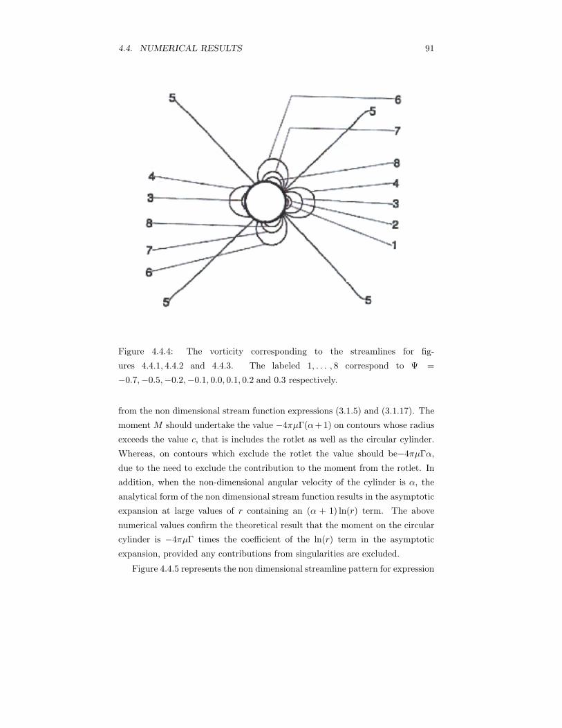
4.4. NUMERICAL RESULTS 91
Figure 4.4.4: The vorticity corresponding to the streamlines for fig-
ures 4.4.1, 4.4.2 and 4.4.3. The labeled 1, . . . , 8 correspond to Ψ =
−0.7,−0.5,−0.2,−0.1, 0.0, 0.1, 0.2 and 0.3 respectively.
from the non dimensional stream function expressions (3.1.5) and (3.1.17). The
moment M should undertake the value −4πμΓ(α+1) on contours whose radius
exceeds the value c, that is includes the rotlet as well as the circular cylinder.
Whereas, on contours which exclude the rotlet the value should be−4πμΓα,
due to the need to exclude the contribution to the moment from the rotlet. In
addition, when the non-dimensional angular velocity of the cylinder is α, the
analytical form of the non dimensional stream function results in the asymptotic
expansion at large values of r containing an (α + 1) ln(r) term. The above
numerical values confirm the theoretical result that the moment on the circular
cylinder is −4πμΓ times the coefficient of the ln(r) term in the asymptotic
expansion, provided any contributions from singularities are excluded.
Figure 4.4.5 represents the non dimensional streamline pattern for expression
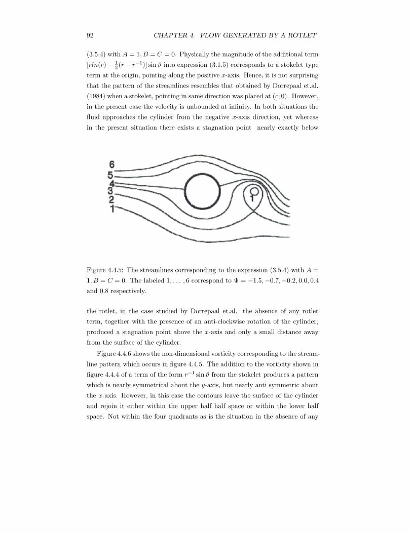
92 CHAPTER 4. FLOW GENERATED BY A ROTLET
(3.5.4) with A = 1, B = C = 0. Physically the magnitude of the additional term
[rln(r) − 12 (r− r−1)] sinϑ into expression (3.1.5) corresponds to a stokelet type
term at the origin, pointing along the positive x-axis. Hence, it is not surprising
that the pattern of the streamlines resembles that obtained by Dorrepaal et.al.
(1984) when a stokelet, pointing in same direction was placed at (c, 0). However,
in the present case the velocity is unbounded at infinity. In both situations the
fluid approaches the cylinder from the negative x-axis direction, yet whereas
in the present situation there exists a stagnation point nearly exactly below
Figure 4.4.5: The streamlines corresponding to the expression (3.5.4) with A =
1, B = C = 0. The labeled 1, . . . , 6 correspond to Ψ = −1.5,−0.7,−0.2, 0.0, 0.4
and 0.8 respectively.
the rotlet, in the case studied by Dorrepaal et.al. the absence of any rotlet
term, together with the presence of an anti-clockwise rotation of the cylinder,
produced a stagnation point above the x-axis and only a small distance away
from the surface of the cylinder.
Figure 4.4.6 shows the non-dimensional vorticity corresponding to the stream-
line pattern which occurs in figure 4.4.5. The addition to the vorticity shown in
figure 4.4.4 of a term of the form r−1 sinϑ from the stokelet produces a pattern
which is nearly symmetrical about the y-axis, but nearly anti symmetric about
the x-axis. However, in this case the contours leave the surface of the cylinder
and rejoin it either within the upper half half space or within the lower half
space. Not within the four quadrants as is the situation in the absence of any
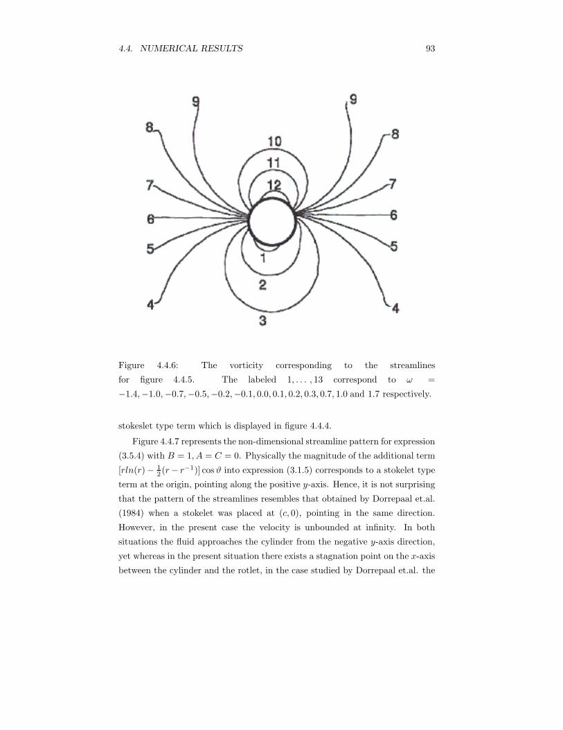
4.4. NUMERICAL RESULTS 93
Figure 4.4.6: The vorticity corresponding to the streamlines
for figure 4.4.5. The labeled 1, . . . , 13 correspond to ω =
−1.4,−1.0,−0.7,−0.5,−0.2,−0.1, 0.0, 0.1, 0.2, 0.3, 0.7, 1.0 and 1.7 respectively.
stokeslet type term which is displayed in figure 4.4.4.
Figure 4.4.7 represents the non-dimensional streamline pattern for expression
(3.5.4) with B = 1, A = C = 0. Physically the magnitude of the additional term
[rln(r)− 12 (r− r−1)] cos ϑ into expression (3.1.5) corresponds to a stokelet type
term at the origin, pointing along the positive y-axis. Hence, it is not surprising
that the pattern of the streamlines resembles that obtained by Dorrepaal et.al.
(1984) when a stokelet was placed at (c, 0), pointing in the same direction.
However, in the present case the velocity is unbounded at infinity. In both
situations the fluid approaches the cylinder from the negative y-axis direction,
yet whereas in the present situation there exists a stagnation point on the x-axis
between the cylinder and the rotlet, in the case studied by Dorrepaal et.al. the
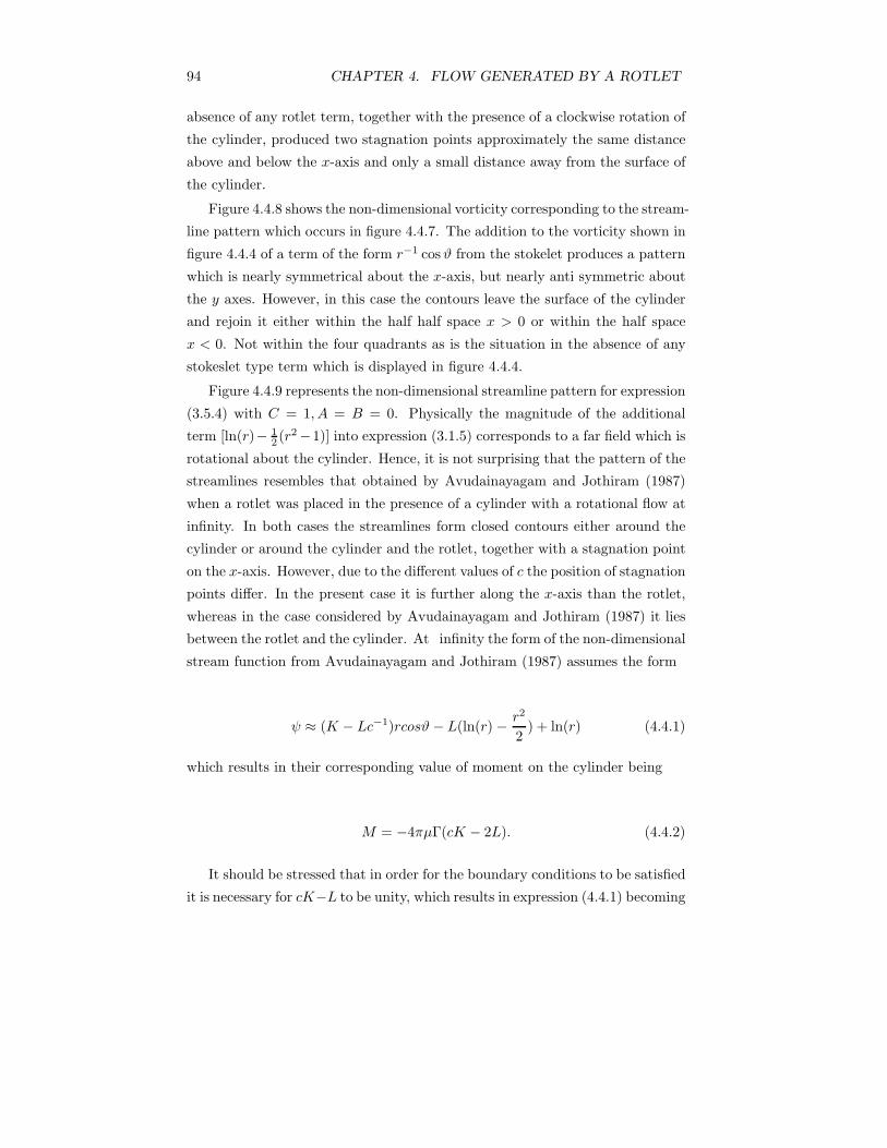
94 CHAPTER 4. FLOW GENERATED BY A ROTLET
absence of any rotlet term, together with the presence of a clockwise rotation of
the cylinder, produced two stagnation points approximately the same distance
above and below the x-axis and only a small distance away from the surface of
the cylinder.
Figure 4.4.8 shows the non-dimensional vorticity corresponding to the stream-
line pattern which occurs in figure 4.4.7. The addition to the vorticity shown in
figure 4.4.4 of a term of the form r−1 cosϑ from the stokelet produces a pattern
which is nearly symmetrical about the x-axis, but nearly anti symmetric about
the y axes. However, in this case the contours leave the surface of the cylinder
and rejoin it either within the half half space x > 0 or within the half space
x < 0. Not within the four quadrants as is the situation in the absence of any
stokeslet type term which is displayed in figure 4.4.4.
Figure 4.4.9 represents the non-dimensional streamline pattern for expression
(3.5.4) with C = 1, A = B = 0. Physically the magnitude of the additional
term [ln(r)− 12 (r2−1)] into expression (3.1.5) corresponds to a far field which is
rotational about the cylinder. Hence, it is not surprising that the pattern of the
streamlines resembles that obtained by Avudainayagam and Jothiram (1987)
when a rotlet was placed in the presence of a cylinder with a rotational flow at
infinity. In both cases the streamlines form closed contours either around the
cylinder or around the cylinder and the rotlet, together with a stagnation point
on the x-axis. However, due to the different values of c the position of stagnation
points differ. In the present case it is further along the x-axis than the rotlet,
whereas in the case considered by Avudainayagam and Jothiram (1987) it lies
between the rotlet and the cylinder. At infinity the form of the non-dimensional
stream function from Avudainayagam and Jothiram (1987) assumes the form
ψ ≈ (K − Lc−1)rcosϑ− L(ln(r) − r2
2) + ln(r) (4.4.1)
which results in their corresponding value of moment on the cylinder being
M = −4πμΓ(cK − 2L). (4.4.2)
It should be stressed that in order for the boundary conditions to be satisfied
it is necessary for cK−L to be unity, which results in expression (4.4.1) becoming
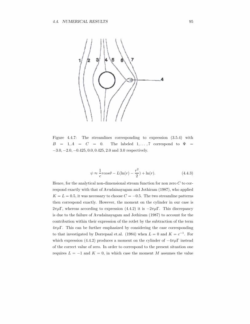
4.4. NUMERICAL RESULTS 95
Figure 4.4.7: The streamlines corresponding to expression (3.5.4) with
B = 1, A = C = 0. The labeled 1, . . . , 7 correspond to Ψ =
−3.0,−2.0,−0.425, 0.0, 0.425, 2.0 and 3.0 respectively.
ψ ≈ 1crcosϑ− L(ln(r) − r2
2) + ln(r). (4.4.3)
Hence, for the analytical non-dimensional stream function for non zero C to cor-
respond exactly with that of Avudainayagam and Jothiram (1987), who applied
K = L = 0.5, it was necessary to choose C = −0.5. The two streamline patterns
then correspond exactly. However, the moment on the cylinder in our case is
2πμΓ, whereas according to expression (4.4.2) it is −2πμΓ. This discrepancy
is due to the failure of Avudainayagam and Jothiram (1987) to account for the
contribution within their expression of the rotlet by the subtraction of the term
4πμΓ. This can be further emphasized by considering the case corresponding
to that investigated by Dorrepaal et.al. (1984) when L = 0 and K = c−1. For
which expression (4.4.2) produces a moment on the cylinder of −4πμΓ instead
of the correct value of zero. In order to correspond to the present situation one
requires L = −1 and K = 0, in which case the moment M assumes the value
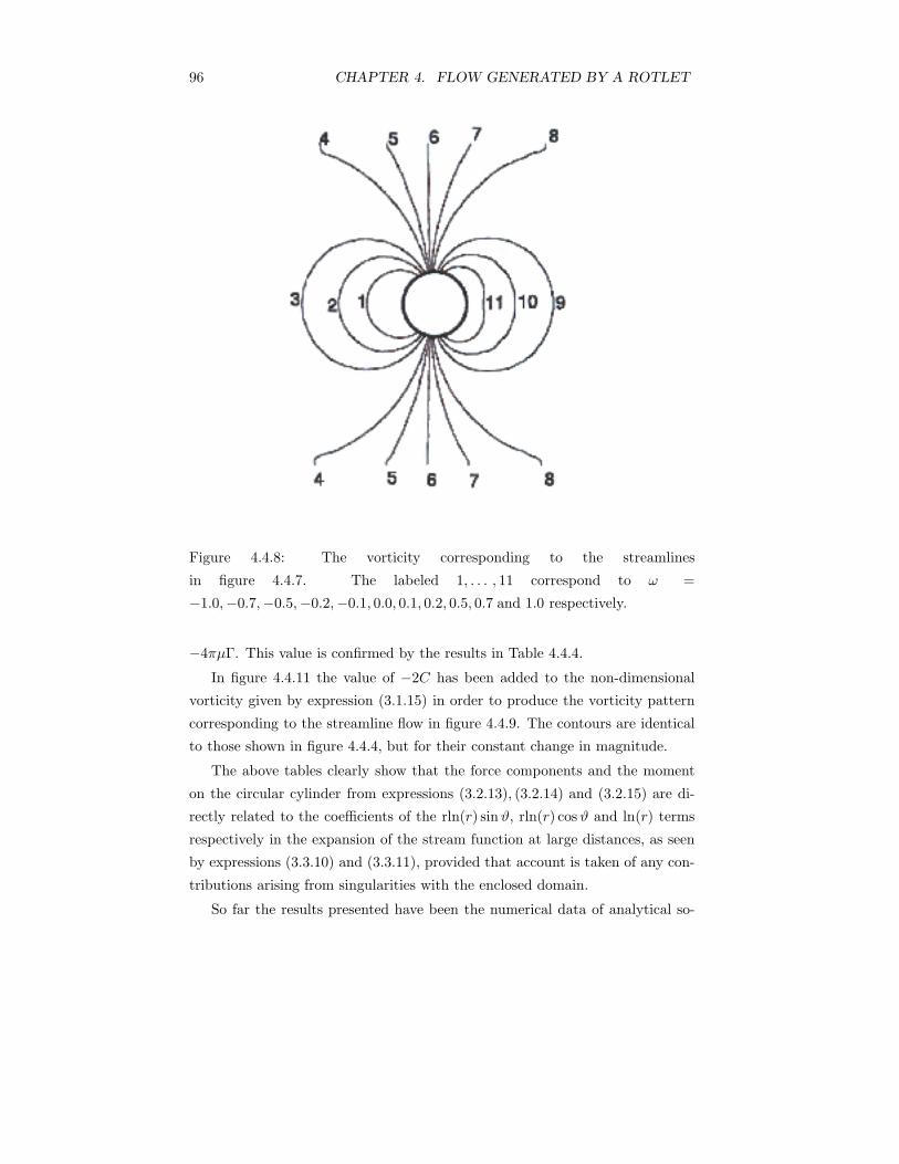
96 CHAPTER 4. FLOW GENERATED BY A ROTLET
Figure 4.4.8: The vorticity corresponding to the streamlines
in figure 4.4.7. The labeled 1, . . . , 11 correspond to ω =
−1.0,−0.7,−0.5,−0.2,−0.1, 0.0, 0.1, 0.2, 0.5, 0.7 and 1.0 respectively.
−4πμΓ. This value is confirmed by the results in Table 4.4.4.
In figure 4.4.11 the value of −2C has been added to the non-dimensional
vorticity given by expression (3.1.15) in order to produce the vorticity pattern
corresponding to the streamline flow in figure 4.4.9. The contours are identical
to those shown in figure 4.4.4, but for their constant change in magnitude.
The above tables clearly show that the force components and the moment
on the circular cylinder from expressions (3.2.13), (3.2.14) and (3.2.15) are di-
rectly related to the coefficients of the rln(r) sinϑ, rln(r) cos ϑ and ln(r) terms
respectively in the expansion of the stream function at large distances, as seen
by expressions (3.3.10) and (3.3.11), provided that account is taken of any con-
tributions arising from singularities with the enclosed domain.
So far the results presented have been the numerical data of analytical so-
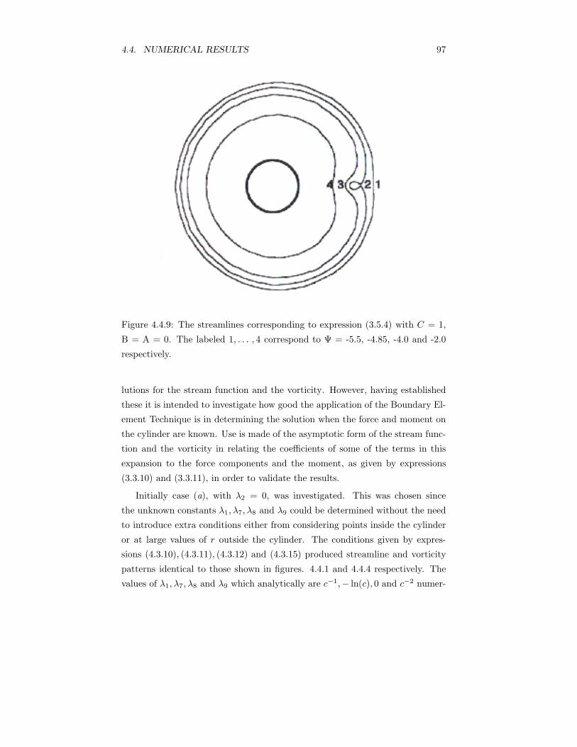
4.4. NUMERICAL RESULTS 97
Figure 4.4.9: The streamlines corresponding to expression (3.5.4) with C = 1,
B = A = 0. The labeled 1, . . . , 4 correspond to Ψ = -5.5, -4.85, -4.0 and -2.0
respectively.
lutions for the stream function and the vorticity. However, having established
these it is intended to investigate how good the application of the Boundary El-
ement Technique is in determining the solution when the force and moment on
the cylinder are known. Use is made of the asymptotic form of the stream func-
tion and the vorticity in relating the coefficients of some of the terms in this
expansion to the force components and the moment, as given by expressions
(3.3.10) and (3.3.11), in order to validate the results.
Initially case (a), with λ2 = 0, was investigated. This was chosen since
the unknown constants λ1, λ7, λ8 and λ9 could be determined without the need
to introduce extra conditions either from considering points inside the cylinder
or at large values of r outside the cylinder. The conditions given by expres-
sions (4.3.10), (4.3.11), (4.3.12) and (4.3.15) produced streamline and vorticity
patterns identical to those shown in figures. 4.4.1 and 4.4.4 respectively. The
values of λ1, λ7, λ8 and λ9 which analytically are c−1,− ln(c), 0 and c−2 numer-
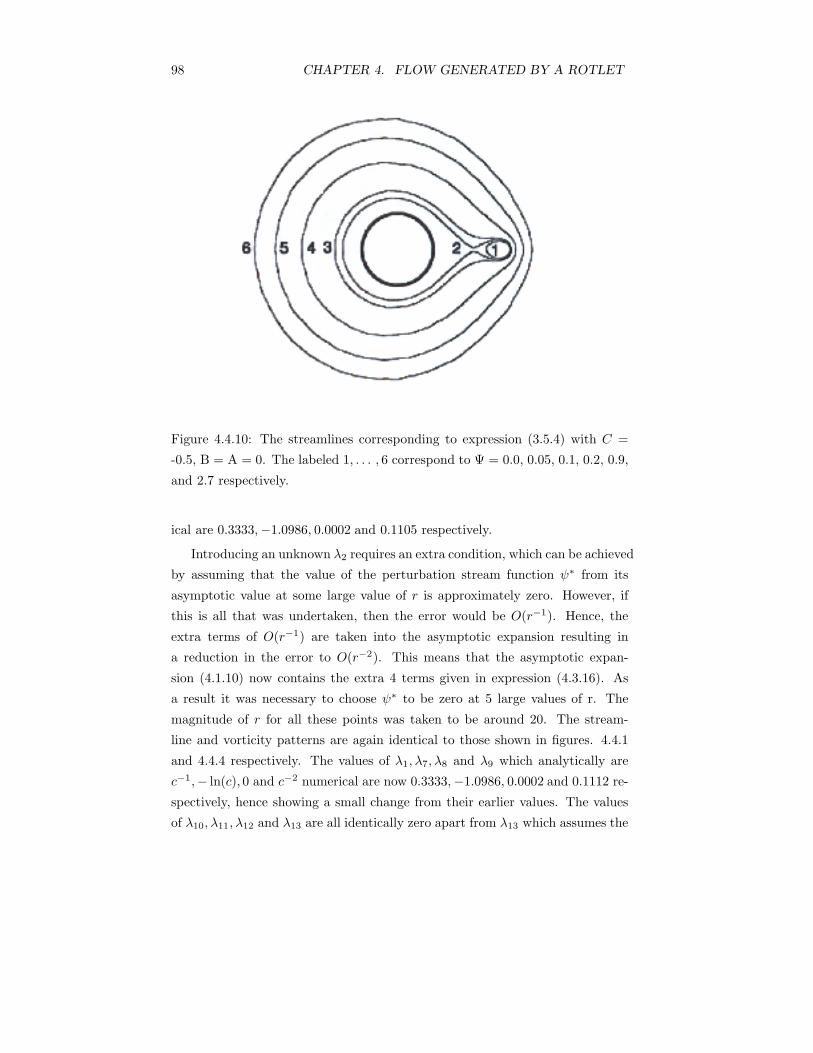
98 CHAPTER 4. FLOW GENERATED BY A ROTLET
Figure 4.4.10: The streamlines corresponding to expression (3.5.4) with C =
-0.5, B = A = 0. The labeled 1, . . . , 6 correspond to Ψ = 0.0, 0.05, 0.1, 0.2, 0.9,
and 2.7 respectively.
ical are 0.3333,−1.0986, 0.0002 and 0.1105 respectively.
Introducing an unknown λ2 requires an extra condition, which can be achieved
by assuming that the value of the perturbation stream function ψ∗ from its
asymptotic value at some large value of r is approximately zero. However, if
this is all that was undertaken, then the error would be O(r−1). Hence, the
extra terms of O(r−1) are taken into the asymptotic expansion resulting in
a reduction in the error to O(r−2). This means that the asymptotic expan-
sion (4.1.10) now contains the extra 4 terms given in expression (4.3.16). As
a result it was necessary to choose ψ∗ to be zero at 5 large values of r. The
magnitude of r for all these points was taken to be around 20. The stream-
line and vorticity patterns are again identical to those shown in figures. 4.4.1
and 4.4.4 respectively. The values of λ1, λ7, λ8 and λ9 which analytically are
c−1,− ln(c), 0 and c−2 numerical are now 0.3333,−1.0986, 0.0002 and 0.1112 re-
spectively, hence showing a small change from their earlier values. The values
of λ10, λ11, λ12 and λ13 are all identically zero apart from λ13 which assumes the
4.4. NUMERICAL RESULTS 99
value c−3. Their corresponding numerical values are −0.0005,−0.0293, 0.0000
and 0.3705 when 40 points are taken around the cylinder, but these become
−0.0001,−0.0148, 0.0000 and 0.3703 when the number of points is increased to
160.
The above inaccuracies arising in the coefficient λ11 can be overcome by
choosing the extra points to be within the cylinder rather than at some large
value of r. In fact since ψ∗ is exactly zero there is no necessity to include the
extra terms from the expression (4.3.16) within the asymptotic expansion of
the stream function. Introducing an extra point within the cylinder to produce
an equation to compensate for the extra unknown coefficient λ2, results in the
same values of λ1, λ7, λ8 and λ9 as given above, together with the value of λ2
as 0.0000.
In case (b) where λ3 = λ6 = 0 the non dimensional force components Fx
and Fy have non zero values - A and B respectively, which is why the coeffi-
cients λ4 and λ5 must be included. Setting A = 1 and B = 0 produced the
streamline and vorticity patterns shown in figures 4.4.5 and 4.4.6 respectively,
with the values of λ1, λ7, λ8 and λ9 unchanged from above, together with the
coefficients λ2 = −0.4961, ( exact value −0.5000), λ4 = 1.0000 and λ5 = 0.0000.
Reversing the values of A and B reverse the values of λ4 and λ5, together with
λ2 = 0.0000, λ1 = −0.1627, ( exact value (c−1 − 12 ) ), λ7, λ8 and λ9 remain-
ing unchanged, and produced the streamlines and vorticity patterns shown in
figures 4.4.7 and 4.4.8.
In case (c) where λ4 = λ5 = 0 the non dimensional moment M has non
zero value −C, which is why the coefficients λ3 and λ6 must be included.
Setting C = 1 produced the streamline and vorticity patterns shown in fig-
ures 4.4.9 and 4.4.11 respectively, with the values of λ8 and λ9 unchanged but
λ1 = 0.3333, λ2 = 0.0000, λ3 = 0.9938( exact value 1), λ6 = −0.5000( exact
value - 12 ), λ7 = −0.5935( exact value − ln(c) + 1
2 ).
In case (d) all the λj , j = 1, . . . . . . , 9 were included in the asymptotic ex-
pansion, hence requiring ψ∗ to be set to zero at 5 points within the cylinder.
With the parameters A,B and C set in turn to their above values the inclusion
of the previous zero coefficients λj , for example in case (b) namely λ3 and λ6,
were numerically calculated to be 0.0000 in all cases. Similarly, the inclusion
of the λ0(r2 ln(r)− r2) term resulted in unchanged values of the coefficients λj ,
for j = 1, . . . .9, together with λ0 = 0.0000.
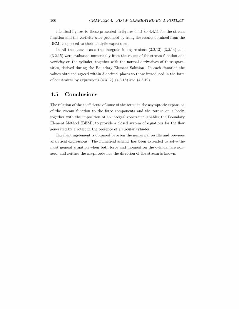
100 CHAPTER 4. FLOW GENERATED BY A ROTLET
Identical figures to those presented in figures 4.4.1 to 4.4.11 for the stream
function and the vorticity were produced by using the results obtained from the
BEM as opposed to their analytic expressions.
In all the above cases the integrals in expressions (3.2.13), (3.2.14) and
(3.2.15) were evaluated numerically from the values of the stream function and
vorticity on the cylinder, together with the normal derivatives of these quan-
tities, derived during the Boundary Element Solution. In each situation the
values obtained agreed within 3 decimal places to those introduced in the form
of constraints by expressions (4.3.17), (4.3.18) and (4.3.19).
4.5 Conclusions
The relation of the coefficients of some of the terms in the asymptotic expansion
of the stream function to the force components and the torque on a body,
together with the imposition of an integral constraint, enables the Boundary
Element Method (BEM), to provide a closed system of equations for the flow
generated by a rotlet in the presence of a circular cylinder.
Excellent agreement is obtained between the numerical results and previous
analytical expressions. The numerical scheme has been extended to solve the
most general situation when both force and moment on the cylinder are non-
zero, and neither the magnitude nor the direction of the stream is known.
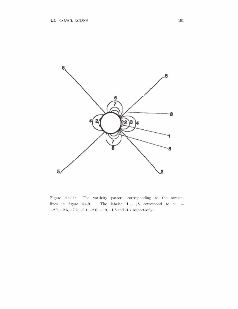
4.5. CONCLUSIONS 101
Figure 4.4.11: The vorticity pattern corresponding to the stream-
lines in figure 4.4.9. The labeled 1, . . . , 8 correspond to ω =
−2.7,−2.5,−2.2,−2.1,−2.0,−1.9,−1.8 and -1.7 respectively.

Chapter 5
THE ROTATION OF TWO
CIRCULAR CYLINDERS
5.1 Introduction
So far our problems have been restricted to Stokes flow in the presence of a single
body, although one could argue that a rotlet, in the presence of either a circular
cylinder or an ellipse, may be regarded as a small rotating circular cylinder and
represents a special case of a two body problem. However, such situations have
been treated as single body problems. In the case of a rotlet outside an ellipse,
Smith (1993) has shown that the Stokes flow at infinity is solid body rotation,
except when the rotlet is placed at one particular position, or to be exact at four
positions due to symmetry, whose coordinates are dependent on the strength of
the rotation of the rotlet. In that special case, like that of a rotlet outside a
circular cylinder, the far field corresponds to that of a uniform stream. It has
been shown by Jeffery (1922) and Smith (1991) that for two body problems a
similar phenomenon occurs, together with a special case.
The paradox which occurred for the above two body problem, (both cylin-
ders of equal radii and rotating with equal speeds, but opposite senses about
parallel axes), when Jeffery (1922) obtained his unusual result of the presence
of a uniform stream at infinity was resolved by the work of Proudman and Pear-
son (1957) and Kaplun and Lagerstrom (1957), where it was shown that such a
Stokes flow was only the far field of an inner solution and that an outer region
103
104 CHAPTER 5. THE ROTATION OF TWO CIRCULAR CYLINDERS
was required where the Navier-Stokes equations, or some modified approxima-
tion of them, are valid. Although at the time Jeffery’s result was known to be
in error due to such a flow having an infinite amount of kinetic energy, whilst
supplied by torques acting on the cylinders for only a finite time so producing
only a finite amount of work. It was probably this unresolved situation which
caused Jeffery to present his solution for only the one particular case when the
cylinders are of the same radii and rotate with equal speeds, but with opposite
senses, about parallel axes, even though he had formulated the general problem
for two cylinders with different radii and different angular velocities.
It was left to Smith (1992) to utilize these expressions to establish that
Jeffery’s result was just a special case of the more general situation where the
far field solution of the Stokes flow corresponds to a rigid body rotation. In fact
Smith was further able to use his solution as the inner boundary condition for the
outer region, where the complete Navier-Stokes equations hold, to produce the
solution in that region. Hence, producing a complete solution over the whole
fluid domain to the problem of two cylinders of different radii and different
angular velocities. This was achieved by means of an inner solution satisfying
the Stokes equation and an outer solution which satisfies the Navier-Stokes
equations. These two solutions being matched at the boundary of the far field
of the inner region, or equivalently the near field of the outer region. This need
for the Stokes solution before one can establish the complete solution over the
whole fluid domain makes the far field form of the Stokes solution considerably
more important that a mere paradox. Before embarking upon a numerical
attempt to establish the Stokes flow using information from the far field of the
inner region in the form of the coefficients of the stream function related to
values of the lift, drag and moment generated on the two bodies, a resume of
the analytical work by Jeffery (1922) and Smith (1991), inter dispersed with
additional information, will be undertaken.
5.2 Co-ordinate System
Jeffery (1922) and Smith (1991) both adopted the bipolar coordinates system
x =A sin(η)
cosh(ξ) − cos(η), y =
A sinh(ξ)cosh(ξ) − cos(η)
, (5.2.1)
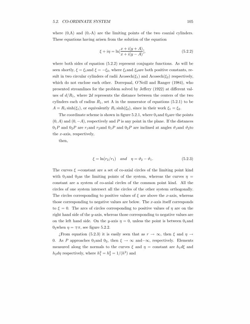
5.2. CO-ORDINATE SYSTEM 105
where (0,A) and (0,-A) are the limiting points of the two coaxial cylinders.
These equations having arisen from the solution of the equation
ξ + iη = ln[x+ i(y +A)x+ i(y −A)
], (5.2.2)
where both sides of equation (5.2.2) represent conjugate functions. As will be
seen shortly, ξ = ξ1and ξ = −ξ2, where ξ1and ξ2are both positive constants, re-
sult in two circular cylinders of radii Acosech(ξ1) and Acosech(ξ2) respectively,
which do not enclose each other. Dorrepaal, O’Neill and Ranger (1984), who
presented streamlines for the problem solved by Jeffery (1922) at different val-
ues of d/R1, where 2d represents the distance between the centers of the two
cylinders each of radius R1, set A in the numerator of equations (5.2.1) to be
A = R1 sinh(ξ1), or equivalently R1 sinh(ξ2), since in their work ξ1 = ξ2.
The coordinate scheme is shown in figure 5.2.1, where 01and 02are the points
(0, A) and (0,−A), respectively and P is any point in the plane. If the distances
01P and 02P are r1and r2and 01P and 02P are inclined at angles ϑ1and ϑ2to
the x-axis, respectively,
then,
ξ = ln(r2/r1) and η = ϑ2 − ϑ1. (5.2.3)
The curves ξ =constant are a set of co-axial circles of the limiting point kind
with 01and 02as the limiting points of the system, whereas the curves η =
constant are a system of co-axial circles of the common point kind. All the
circles of one system intersect all the circles of the other system orthogonally.
The circles corresponding to positive values of ξ are above the x-axis, whereas
those corresponding to negative values are below. The x-axis itself corresponds
to ξ = 0. The arcs of circles corresponding to positive values of η are on the
right hand side of the y-axis, whereas those corresponding to negative values are
on the left hand side. On the y-axis η = 0, unless the point is between 01and
02when η = ∓π, see figure 5.2.2.
¿From equation (5.2.3) it is easily seen that as r → ∞, then ξ and η →0. As P approaches 01and 02, then ξ → ∞ and−∞, respectively. Elements
measured along the normals to the curves ξ and η = constant are h1dξ and
h2dη respectively, where h21 = h2
2 = 1/(h2) and
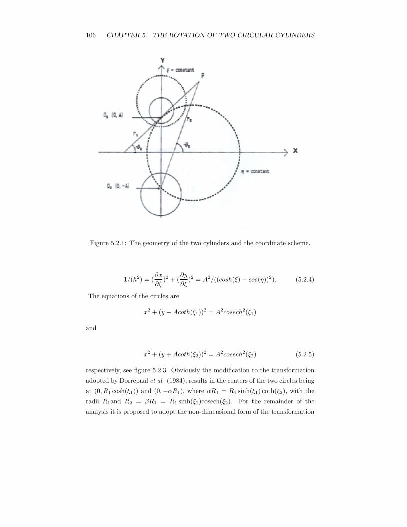
106 CHAPTER 5. THE ROTATION OF TWO CIRCULAR CYLINDERS
Figure 5.2.1: The geometry of the two cylinders and the coordinate scheme.
1/(h2) = (∂x
∂ξ)2 + (
∂y
∂ξ)2 = A2/((cosh(ξ) − cos(η))2). (5.2.4)
The equations of the circles are
x2 + (y −Acoth(ξ1))2 = A2cosech2(ξ1)
and
x2 + (y +Acoth(ξ2))2 = A2cosech2(ξ2) (5.2.5)
respectively, see figure 5.2.3. Obviously the modification to the transformation
adopted by Dorrepaal et al. (1984), results in the centers of the two circles being
at (0, R1 cosh(ξ1)) and (0,−αR1), where αR1 = R1 sinh(ξ1) coth(ξ2), with the
radii R1and R2 = βR1 = R1 sinh(ξ1)cosech(ξ2). For the remainder of the
analysis it is proposed to adopt the non-dimensional form of the transformation
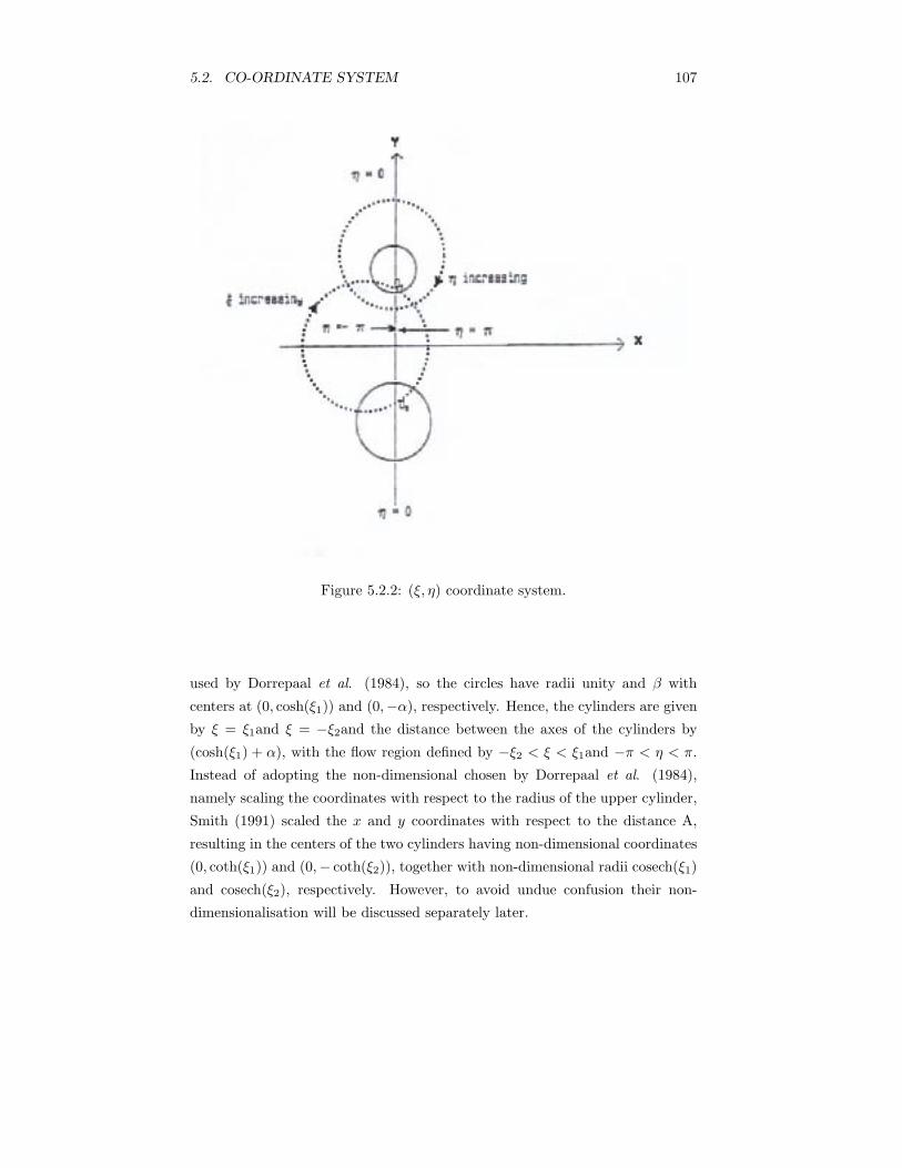
5.2. CO-ORDINATE SYSTEM 107
Figure 5.2.2: (ξ, η) coordinate system.
used by Dorrepaal et al. (1984), so the circles have radii unity and β with
centers at (0, cosh(ξ1)) and (0,−α), respectively. Hence, the cylinders are given
by ξ = ξ1and ξ = −ξ2and the distance between the axes of the cylinders by
(cosh(ξ1) + α), with the flow region defined by −ξ2 < ξ < ξ1and −π < η < π.
Instead of adopting the non-dimensional chosen by Dorrepaal et al. (1984),
namely scaling the coordinates with respect to the radius of the upper cylinder,
Smith (1991) scaled the x and y coordinates with respect to the distance A,
resulting in the centers of the two cylinders having non-dimensional coordinates
(0, coth(ξ1)) and (0,− coth(ξ2)), together with non-dimensional radii cosech(ξ1)
and cosech(ξ2), respectively. However, to avoid undue confusion their non-
dimensionalisation will be discussed separately later.
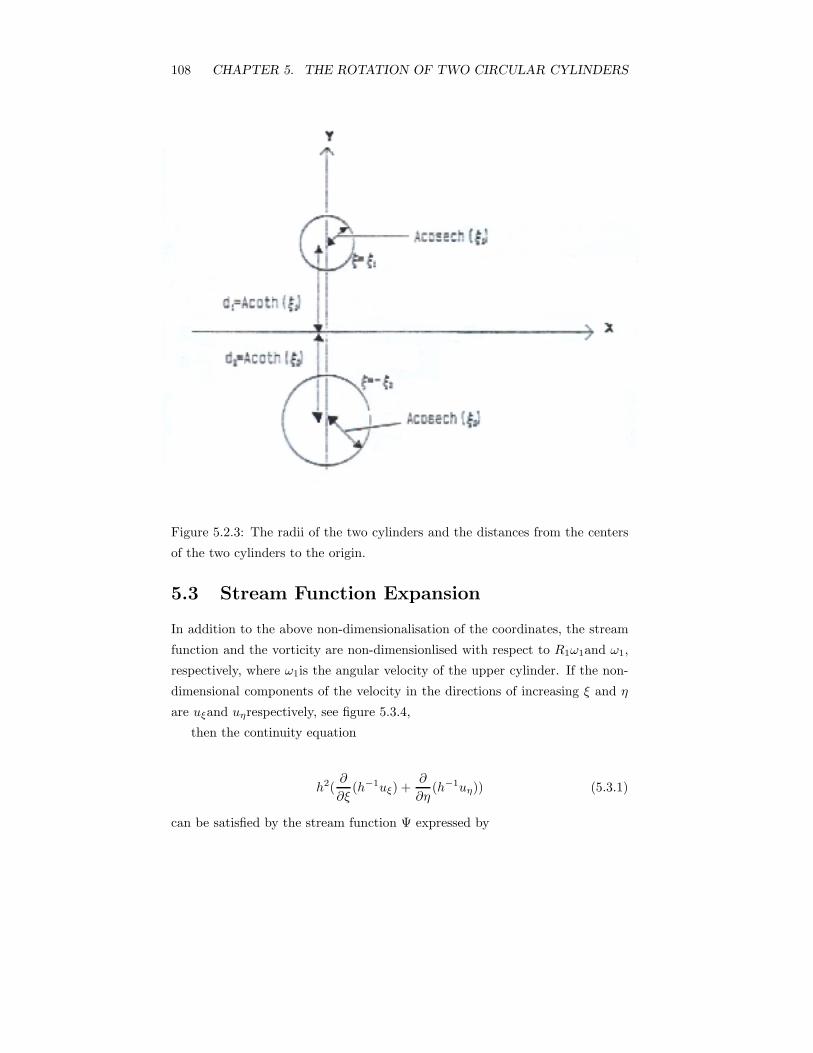
108 CHAPTER 5. THE ROTATION OF TWO CIRCULAR CYLINDERS
Figure 5.2.3: The radii of the two cylinders and the distances from the centers
of the two cylinders to the origin.
5.3 Stream Function Expansion
In addition to the above non-dimensionalisation of the coordinates, the stream
function and the vorticity are non-dimensionlised with respect to R1ω1and ω1,
respectively, where ω1is the angular velocity of the upper cylinder. If the non-
dimensional components of the velocity in the directions of increasing ξ and η
are uξand uηrespectively, see figure 5.3.4,
then the continuity equation
h2(∂
∂ξ(h−1uξ) +
∂
∂η(h−1uη)) (5.3.1)
can be satisfied by the stream function Ψ expressed by
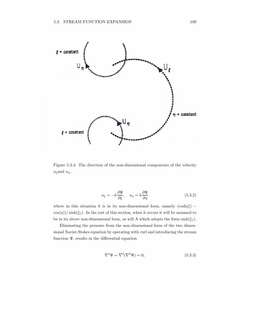
5.3. STREAM FUNCTION EXPANSION 109
Figure 5.3.4: The direction of the non-dimensional components of the velocity
uξand uη.
uξ = −h∂Ψ∂ξ
, uη = h∂Ψ∂η
(5.3.2)
where in this situation h is in its non-dimensional form, namely (cosh(ξ) −cos(η))/ sinh(ξ1). In the rest of this section, when h occurs it will be assumed to
be in its above non-dimensional form, as will A which adopts the form sinh(ξ1).
Eliminating the pressure from the non-dimensional form of the two dimen-
sional Navier-Stokes equation by operating with curl and introducing the stream
function Ψ, results in the differential equation
∇4Ψ = ∇2(∇2Ψ) = 0, (5.3.3)
110 CHAPTER 5. THE ROTATION OF TWO CIRCULAR CYLINDERS
where
∇2Ψ = ∇.(∇Ψ) = h2
(∂2
∂ξ2+
∂2
∂η2
)(5.3.4)
However, on changing the dependent variable from Ψ to hΨ, expression (5.3.4)
becomes
∇2Ψ = [h(∂2
∂ξ2+
∂2
∂η2) − 2sinh(ξ)
∂
∂ξ− 2sin(η)
∂
∂η
+ cosh(ξ) + cos(η)](hΨ),(5.3.5)
which on repeating the operation, plus a small amount of simplification, results
in equation (5.3.3) becoming a linear partial differential equation with constant
coefficients, namely[∂4
∂ξ4+ 2
∂4
∂ξ2∂η2+
∂4
∂η4− 2
∂2
∂ξ2+ 2
∂2
∂η2+ 1
](hΨ) = 0. (5.3.6)
Seeking a solution of equation (5.3.6) of the form hΨ = f(ξ) cos(nη) or f(ξ) sin(nη),
the periodicity, necessary from the geometry of the problem, gives rise to the
ordinary differential equation
[d4
dξ4− 2(n2 + 1)
d2
dξ2+ n4 − 2n2 + 1
]f(ξ) = 0. (5.3.7)
The solution of equation (5.3.7) has the form
f(ξ) = An cosh((n+ 1)ξ) +Bn cosh((n− 1)ξ) + Cn sinh((n+ 1)ξ)
+Dn sinh((n− 1)ξ), for n ≥ 2,(5.3.8)
f(ξ) = A1 cosh(2ξ) +B1 + C1 sinh(2ξ) +D1ξ, for n = 1, (5.3.9)
and
f(ξ) = A0 cosh(ξ) +B0ξ cosh(ξ) + C0 sinh(ξ) +D0ξ sinh(ξ), for n = 0,
(5.3.10)
where Ai, Bi, Ci and Difor i = 0, 1, . . . . . . . are the constants of integration.
5.3. STREAM FUNCTION EXPANSION 111
Due to the general solution of equation (5.3.6) being
hΨ = exp(±ξ)f(ξ ± iη) (5.3.11)
the terms ξ sin(η), ξ cos(η), ξ cosh(ξ) and ξ sinh(η) in expressions (5.3.8), (5.3.9)
and (5.3.10) result in the addition solutions
hΨ = η, (5.3.12)
where E,F,G and H are unknown constants. However, these solutions can
be rejected due to the requirement of single-valuedness of the solution. In the
present problem the stream function is an even function in η, as is the function
h, and therefore all the terms involving sin(nη) may be omitted. Thus hΨ
assumes the form
hΨ = A0cosh(ξ) +B0ξcosh(ξ) + C0sinh(ξ) +D0ξsinh(ξ)
+ [A1cosh(2ξ) +B1 + C1sinh(2ξ) +D1ξ]cos(η)
+∞∑
n=2
[Ancosh((n+ 1)ξ) +Bnξcosh((n− 1)ξ)
+ Cnsinh((n+ 1)ξ) +Dnξsinh((n− 1)ξ)]cos(nη).
(5.3.13)
At this point it should be observed that Jeffery (1922) noted that the above
series may converge only for positive or for negative values of ξ. That is to
say that different expansions of hΨ on either side of ξ = 0 may be required.
However, as will be discussed later he was able to justify his choice of hΨ for
the domain ξ > 0 and to establish a solution for the whole fluid space using a
symmetry argument. From the component form of the Navier Stokes equation
it is readily seen that both the pressure p and the expression ∇2Ψ satisfy the
Cauchy-Riemann equations, which means that the function p+i∇2Ψ is a regular
function of z = x + iy, so x and y can only occur in the combination x + iy.
However, equation (2) clearly shows that p + i∇2Ψ must also be a regular
function of ζ = ξ+ iη. Evaluating ∇2Ψ by substituting expression (18) into the
right hand side of equation (10) results in a term (B0 +D1)ξ, which means that
the pressure p must contain a term −(B0 +D1)η. The inclusion of such a term
would violate the condition regarding the single-valuedness of the velocity and
the pressure, hence it is necessary for the constraint
112 CHAPTER 5. THE ROTATION OF TWO CIRCULAR CYLINDERS
(B0 +D1) = 0, (5.3.14)
to be applied.
5.4 Boundary Bonditions
Jeffery showed that a solution of the biharmonic equation ∇4Ψ = 0 in the region
−ξ2 < ξ < ξ1,−π < η < π which satisfies the no slip condition on ξ = −ξ2and
on ξ = ξ1is given by
hΨ = A0 cosh(ξ) +B0ξ cosh(ξ) + C0 sinh(ξ) +D0ξ sinh(ξ)
+ (A1 cosh(2ξ) +B1 + C1 sinh(2ξ) +D1ξ) cos(η).(5.4.1)
The zero normal velocity boundary conditions are that on
ξ = −ξ2, Ψ = −Ψ2; (5.4.2)
whilst on
ξ = ξ1, Ψ = Ψ1. (5.4.3)
This choice of Ψ = −Ψ2on ξ = −ξ2has been taken to coincide with that taken
by Smith (1991), who followed Jeffery (1922), since the latter had employed that
on ξ = 0 the value of Ψ was zero, so making his value of Ψ = −Ψ1on ξ = −ξ2by
the symmetry of the particular case studied.
The components of the non-dimensional fluid velocity in terms of the non-
dimensional stream function in expression (5.3.2) can be rewritten in terms of
the dependent variable hΨ as follows
uξ = −h∂Ψ∂η
= −[∂(hΨ)∂η
− ΨA
sin(η)], (5.4.4)
uη = h∂Ψ∂ξ
= −[∂(hΨ)∂ξ
− ΨA
sinh(ξ)], (5.4.5)
5.4. BOUNDARY BONDITIONS 113
where uξand uηare in the directions of ξ and η increasing. This means that on
ξ = ξ1, uη = −1, and by substituting A = sinh(ξ1), one obtains
∂
∂ξ(hΨ) = Ψ1 − 1. (5.4.6)
An alternative way of expressing this equation is
∂Ψ∂ξ
= −1/h = − sinh(ξ1)/[cosh(ξ!) − cos(η)], (5.4.7)
which agrees, but for the sign, with the condition employed by Dorrepaal et
al. (1984). The sign difference arising due to the upper cylinder rotating in
the clockwise direction in the work of Dorrepaal et al. (1984), but in the anti-
clockwise in that of Smith (1992) and of Jeffery (1922). Also
on ξ = −ξ2, uη = −(ω2/ω1) sinh(ξ1)cosech(ξ2) = −βω2/ω1,
= −R2ω2/(R1ω1),(5.4.8)
which produces
∂
∂ξ(hΨ) = Ψ2sinh(ξ2)/[sinh(ξ1) − (ω2/ω1)sinh()ξ1cosech(ξ2)] (5.4.9)
= ψ2/β − βω2/ω1. (5.4.10)
Again this expression may be written as
∂Ψ∂ξ
= −βω2/(hω1), (5.4.11)
= − sinh(ξ1)cosech(ξ2)ω2/[ω1(cosh(ξ2) − cos(η))] (5.4.12)
which with ξ1 = ξ2, that is two identical cylinders, and ω1 = ω2, reduces to that
adopted by Dorrepaal et al. (1984), but for the sign. With Ψ1 = Ψ2, ω1 = ω2and
ξ1 = ξ2, then equations (5.4.6) and (5.4.9) are identical, and agree with the
conditions, apart from the difference of sign, applied by Dorrepaal et al. (1984).
The angular velocities of the two cylinders in the above have been taken as
ω = ω1k on ξ = ξ1 and ω = −ω2k on ξ = −ξ2. (5.4.13)
114 CHAPTER 5. THE ROTATION OF TWO CIRCULAR CYLINDERS
5.5 Linear Equation of the Boundary Conditions
The constant values of the stream function on ξ = ξ1and ξ = −ξ2are Ψ1and
−Ψ2, respectively, with Ψ1 − (−Ψ2) = Ψ1 + Ψ2, the difference between the
stream function on the two cylinders being an independent quantity. Hence,
the nine unknowns are Ψ1 + Ψ2, Aj , Bj , Cj , Dj , where j = 0 and 1, whilst the
nine equations necessary to determine these values are the constraint equation
(5.3.14), plus the eight equations arising from substituting the stream function
from expression (5.4.1) into the boundary conditions (5.4.2), (5.4.3), (5.4.6) and
(5.4.9) and equating the coefficient of the cos(η) term and that of the constant
term both to zero, so producing
A0 cosh(ξ1) +B0ξ1 cosh(ξ1) + C0 sinh(ξ1) +D0ξ1 sinh(ξ1)
= Ψ1 cosh(ξ1)/(sinh(ξ1)).(5.5.1)
A1 cosh(2ξ1) +B1 + C1 sinh(2ξ1) +D1ξ1 = −Ψ1/(sinh(ξ1)), (5.5.2)
A0 sinh(ξ1) + B0ξ1 sinh(ξ1) + C0 cosh(ξ1)
+D0(ξ1 cosh(ξ1) + sinh(ξ1) = Ψ1 − 1.(5.5.3)
2A1 sinh(2ξ1) + 2C1 cosh(2ξ1) +D1 = 0, (5.5.4)
A0 cosh(ξ2) −B0ξ2 cosh(ξ2) − C0 sinh(ξ2) +D0ξ2 sinh(ξ2)
= −Ψ2 cosh(ξ2)/(sinh(ξ1)).(5.5.5)
A1 cosh(2ξ2) +B1 − C1 sinh(2ξ2) −D1ξ2) −D1ξ2 = Ψ2/(sinh(ξ1)), (5.5.6)
A0 cosh(ξ2) −B0ξ2 cosh(ξ2) − C0 sinh(ξ2) +D0ξ2 sinh(ξ2)
= −Ψ2 cosh(ξ2)/(sinh(ξ1)).(5.5.7)
−2A1 sinh(2ξ2) + 2C1 cosh(2ξ2) +D1 = 0. (5.5.8)
Although the non-dimensionalisation in the above work has followed that of
Dorrepaal et al. (1984), it is possible to adopt the procedure chosen by both

5.5. LINEAR EQUATION OF THE BOUNDARY CONDITIONS 115
Jeffrey (1922) and Smith (1991). There the length non-dimensionalisation was
undertaken with respect to the parameter A, where 2A represents the distance
between the limiting points of the two cylinders in the bipolar coordinate sys-
tem, instead of with respect to the radius R1of the upper cylinder. With such
a non-dimensionalisation the centers of the upper and lower cylinders are at
(0, coth(ξ1)) and (0,− coth(ξ2)) respectively, whilst the radii are cosech(ξ1)
and cosech(ξ2). In addition the non-dimensional form of the function h will
be (cosh(ξ) − cos(η)). Application of the form for hΨ expressed in equation
(5.4.1) into the boundary conditions on the two cylinders produces, in this non-
dimensional system, a modified form of the equations (5.5.1) to (5.5.8), namely
A0 cosh(ξ1) +B0ξ1 cosh(ξ1) + C0 sinh(ξ1) +D0ξ1 sinh(ξ1) = Ψ1 cosh(ξ1).
(5.5.9)
A1 cosh(2ξ1) +B1 + C1 sinh(2ξ1) +D1ξ1 = −Ψ1, (5.5.10)
A0 sinh(ξ1) +B0(ξ1 sinh(ξ1) + cosh(ξ1)) + C0 cosh(ξ1)
+D0(ξ1 cosh(ξ1) + sinh(ξ1)) = Ψ1 sinh(ξ1) − cosech(ξ1),(5.5.11)
2A1 sinh(2ξ1) + 2C1 cosh(2ξ1) +D1 = 0, (5.5.12)
A0 cosh(ξ2) −B0ξ2 cosh(ξ2) − C0 sinh(ξ2) +D0ξ2 sinh(ξ2) = −Ψ2 cosh(ξ2).
(5.5.13)
A1 cosh(2ξ2) +B1 − C1 sinh(2ξ2) −D1ξ2) −D1ξ2 = Ψ2 (5.5.14)
A0 sinh(ξ2) +B0(ξ2 sinh(ξ2) + cosh(ξ2)) + C0 cosh(ξ2)
+D0(ξ2 cosh(ξ2) + sinh(ξ2)) = Ψ2 sinh(ξ2) − (ω2
ω1)cosech(ξ2),
(5.5.15)
−2A1 sinh(2ξ2) + 2C1 cosh(2ξ2) +D1 = 0. (5.5.16)
If the stream function and the coefficients Aj , Bj , Cjand Dj , where j = 0 and
1, in equations (5.5.9) to (5.5.16) are redefined as sinh2(ξ1) times the stream
function value and sinh(ξ1) times the coefficients, respectively, then equations
116 CHAPTER 5. THE ROTATION OF TWO CIRCULAR CYLINDERS
(5.5.1) to ((5.5.8) are identical with the equations (5.5.9) to (5.5.16). This means
that the coefficients obtained by solving the non-dimensional set of equations in
Smith (1991), namely equations (5.5.9) to (5.5.16), can be seen on multiplication
by sinh(ξ1) to give identical values to those obtained by solving equations (5.5.1)
to (5.5.8). Likewise, multiplication by sinh2(ξ1) of the streamfunction in Smith
(1991) produces the form obtained by Dorrepaal et al. (1984).
Returning to equations (5.5.1) to (5.5.8), then the work of Dorrepaal et al.
(1984), with the rotation of both cylinders reversed in order to agree with the
directions chosen by Jeffery (1922) and by Smith (1991), shows that there is an
analytical solution when ξ1 = ξ2and ω1 = ω2, namely,
[cosh(ξ) − cos(η)
sinh(ξ)]Ψ = hΨ
= A0 cosh(ξ) +B0ξ cosh(ξ) + C0 sinh(ξ) +D0ξ sinh(ξ)
+ (A1 cosh(2ξ) +B1 + C1 sinh(2ξ) +D1ξ) cos(η),
(5.5.17)
where
A0 = A1 = B1 = D0 = 0, B0 = −D1 = −(coth(2ξ1))/ sinh(ξ1),
C0 = (coth(ξ1))/(2 sinh(ξ1)), C1 = −(cosech(2ξ1))/(2 sinh(ξ1)),(5.5.18)
which agree, on division by sinh(ξ1) with the coefficients presented in Jeffery
(1922). These results also highlight the fact that the stream functions in the
work in Jeffery (1922), or in Smith (1991), and in Dorrepaal et al. (1984) differ
by a factor sinh2(ξ1).
In addition to the solutions by Jeffery (1922) and by Dorrepaal et al. (1984)
for the case of cylinders of equal radii rotating with equal speeds but in opposite
senses, Smith (1991) has solved equations (5.5.9) to (5.5.17) for the most general
situation, namely different radii and different angular velocities. Unfortunately,
the expressions for the various coefficients in the function hΨ are rather lengthy
and as a result only those combinations necessary for the evaluations of the form
of the stream function at large distances from the cylinders and the torques on
the two cylinders are presented. Rather than produce algebraic expressions for
the coefficients, the two sets of equations (5.5.1) to (5.5.8) and equations (5.5.9)
to (5.5.16) have been solved numerically for various cylinder radii and angular
velocities, and the values for the combinations of the constants, presented in
Smith (1991), checked. Streamlines have been drawn for some of these radii and
5.6. ASYMPTOTIC FORM OF THE STREAM FUNCTION 117
angular velocities and are shown in figures 5.5.5 and 5.5.6. These cases included
the special situation when the value of (A0 + A1 + B1) is zero, since, as will
be seen later, the solution for this special value should at large distances from
the cylinders correspond to a uniform stream rather than solid body rotation
as occurs for all non zero values of this parameter. Corresponding to each
streamline pattern, the vorticity distribution, resulting from the substitution of
the expression for hΨ, given by equation (5.4.1), into equation (5.3.5), producing
the non-dimensional vorticity
ω = ∇2ψ = (cosh(ξ) − cos(η)) (p2 + (q2 − q0) cos(η))
− 2 sinh(ξ)(p1 + q1 cos(η)) + q0 sin2(η)
+ (cosh(ξ) + cos(η))(p0 + q0 cos(η)),
(5.5.19)
where
p0 = A0cosh(ξ) +B0ξcosh(ξ) + C0sinh(ξ) +D0ξsinh(ξ),
q0 = A1cosh(2ξ) +B1 + C1sinh(2ξ) +D1ξ,
p1 = A0sinh(ξ) +B0(cosh(ξ) + ξsinh(ξ)) + C0cosh(ξ)
+D0(sinh(ξ) + ξcosh(ξ)),
q1 = 2A1sinh(2ξ) + 2C1cosh(2ξ) +D1,
p2 = A0cosh(ξ) +B0(2sinh(ξ) + ξcosh(ξ)) + C0sinh(ξ)
+D0(2cosh(ξ) + ξsinh(ξ),
q2 = 4A1cosh(2ξ) + 4C1sinh(2ξ).
⎫⎪⎪⎪⎪⎪⎪⎪⎪⎪⎪⎪⎪⎪⎪⎬⎪⎪⎪⎪⎪⎪⎪⎪⎪⎪⎪⎪⎪⎪⎭
(5.5.20)
has been presented in Figures 5.5.6.
5.6 Asymptotic Form of the Stream Function
It seems that now is the appropriate time to investigate the behavior of the
streamfunction at large distances from the cylinder, as documented by Smith
(1991). It has already been mentioned that the condition of x, y → ∞ requires
ξ, η → 0, which results in
(ξ2 + η2)Ψ/ sinh(ξ1) � 2(A0 +A1 +B1) + 2(C0 + 2C1)ξ
+ (A0 + 2D0 + 4A1)ξ2/2 − (A1 +B1)η2/2 +O(((ξ2 + η2)3/2),(5.6.1)
118 CHAPTER 5. THE ROTATION OF TWO CIRCULAR CYLINDERS
where
Δ(A0+A1 +B1) = (ξ1 + ξ2)(ω1sinh2(ξ2) − ω1 sinh2(ξ1)) sinh(ξ1), (5.6.2)
Δ(C0 + 2C1) = ω1sinh(ξ1)sinh(ξ2)[(ξ1 + ξ2)sinh(ξ1)cosech(ξ1 + ξ2)
+ sinh(ξ2) + (ξ1 + ξ2)cosh(ξ2) − ξ2sinh(ξ1 + ξ2)cosech(ξ1)]
+ ω2sinh2(ξ1)[(ξ1 + ξ2)sinh(ξ2)cosech(ξ1 + ξ2) + sinh(ξ1)
+ (ξ1 + ξ2)cosech(ξ1) − ξ1sinh(ξ1 + ξ2)cosech(ξ2)]
(5.6.3)
with
Δ = (ξ1 + ξ2){sinh2(ξ1) + sinh2(ξ2)}
+ 2sinh(ξ1)sinh(ξ2)sinh(ξ1 + ξ2).(5.6.4)
As at small values of ξ and η, the non-dimensional values x and y take the form
x � 2η sinh(ξ1)/(ξ2 + η2), (5.6.5)
and
y � 2ξ sinh(ξ1)/(ξ2 + η2), (5.6.6)
it follows that
Ψ � (A0 +A1 +B1)(x2 + y2)/(2 sinh(ξ1)) + (C0 + 2C1)y
+ sinh(ξ1) {−(A0 + 2D0 + 5A1 +B1)cos(2ϑ)} /2
+ sinh(ξ1) {(A0 + 2D0 + 3A1 −B1)} /2
(5.6.7)
as x and y → ∞. Expression (5.6.7) can easily be changed to its form presented
in Smith (1992). However, care must be taken to apply not only the modification
necessary between the stream functions and the coefficients A0, etc. in the two
different non-dimensionalised systems but also to note that x and y are non-
dimensional. The non-dimensionalisation being with respect to R1in the present
work, and in that by Dorrepaal et al. (1984), whereas in Smith (1991) it is with
respect to A, where A = R1 sinh(ξ1). The O(1) term in the asymptotic series
of the stream function at large distances from the cylinder was not presented
by Smith (1991), and under normal circumstances would be unnecessary since
5.6. ASYMPTOTIC FORM OF THE STREAM FUNCTION 119
it neither conveys the strength of the solid body rotation, if present, nor the
magnitude of the uniform stream. However, in later work it will provide a useful
check of the accuracy of the results since then the stream function is considered
as the sum of its value at infinity plus a perturbation. The perturbation term
being finite in the vicinity of the cylinders but tending to zero at infinity. A
non-zero value of the leading order term in expression (5.6.7), (A0 +A1 +B1)r2,
clearly indicates that, based on the Stokes equation, there is solid body rotation
far from the cylinders. This fact appeared to have been overlooked by all workers
on this problem prior to Smith (1992) and probably arose due to the physical
situations being studied being restricted to cylinders of equal radii, with angular
velocities of equal magnitude but opposite senses. If one views equation (5.6.2),
excluding the situation that either ξ1or ξ2are zero, which means that neither of
the cylinders is a plane and hence in reality possess zero angular velocity, then
it is only possible to have zero rotation at infinity when
ω1 sinh2(ξ2) = ω2 sinh2(ξ1). (5.6.8)
Multiplication of equation (5.6.8) by the dimensional A2, namely R21 sinh2(ξ1),
results in the more physically recognizable relationship, namely
ω1R21 = ω2R
22. (5.6.9)
This requires that the angular momenta of the two cylinders must exactly bal-
ance, and in such a situation there is just a uniform stream at infinity in the
direction perpendicular to the line of centers of the cylinders. The actual direc-
tion corresponding to that of the direction the surfaces of the cylinders when
they meet the line connecting their centers. Hence, in the present case when
ω1and ω2in expressions (5.4.13) are both positive the stream will be directed
parallel to the x-axis and in the direction of x increasing. Since Dorrepaal
et al. (1984) reversed both these directions of rotation, it follows that their
stream should have been directed in the direction of x decreasing. However, the
opposite direction appears to have been their choice.
120 CHAPTER 5. THE ROTATION OF TWO CIRCULAR CYLINDERS
5.7 Validation of the Expansions for hΨ
Before embarking into a detailed discussion regarding the forces and the torques
acting on the cylinders it seems an appropriate place to refer back to the point
mentioned earlier, and discussed by Jeffery (1922), relating to whether different
expansions are required in the separate domains ξ > 0 and ξ < 0 when one of
the two cylinders fails to enclose the other. However, Jeffery (1922) rather than
pursue the different expansions on opposite sides of the plane ξ = 0 opted for
cylinders of equal radii, rotating with equal speeds but in opposite senses. This
meant that by using a symmetry argument, together with the stream function
being a constant and the shearing stress vanishing on the plane ξ = 0, it was
possible to obtain a solution in the whole fluid domain from an expansion for the
region ξ > 0 only. Jeffery (1922) found that the most general form of expression
(5.3.13) which satisfied the boundary conditions on the upper cylinder and the
boundary conditions on the plate ξ = 0 was that presented in expression (5.4.1).
The question as to whether the expansion (5.3.13) is valid on the plane ξ = 0,
in other words ”Is it absolutely and uniformly convergent”, was simply assumed
for the matter of obtaining the solution, with a full physical argument presented
as to its validity. Jeffery (1922) concluded that since it was possible to solve
uniquely the problem of a cylinder rotating in a viscous fluid contained within
a non-concentric vessel whose inner surface was smooth and so unable to exert
any tangential stress on the fluid, then by allowing the radius of the outer vessel
to then become infinitely large that solution should correspond to his result,
found with the help of symmetry, in the upper half plane. As the flow in the
contained vessel was unique and did tend at large distances from the rotating
cylinder to that already found by using expansion (5.4.1) for the region ξ > 0,
then the use of the more general form of expansion (5.3.13), namely expansion
(5.4.1), on the boundary ξ = 0, must, regarding its convergence, be valid. Both
Dorrepaal et al. (1984) and Smith (1991) assumed that an expansion of the form
in expression (5.4.1), rather than that in expression (5.3.13), was acceptable
and that there was no need for different expansions in the regions ξ > 0 and
ξ < 0. However, it could be argued that Dorrepaal et al. (1984) had the stronger
grounds for this assumption, based upon the fact that Jeffery (1922) had already
found such a solution for the region ξ ≥ 0 and could extend, by symmetry,
that solution to the region ξ < 0. For Smith (1991), this argument was no
5.7. VALIDATION OF THE EXPANSIONS FOR HΨ 121
longer possible due to the complete lack of symmetry in the physical situations
being investigated. However, Jeffery (1920), in a paper entitled, ”Plane stress
and plane strain in bipolar coordinates”, outlined the restrictions under which
a single expansion like expression (5.3.13), and hence like expression (5.4.1),
might be valid throughout the whole region. If the plate was such that it
contained two circular holes, neither of which enclosed the other, then it was
possible to establish that provided the forces and torque acting over the two
circular boundaries were in equilibrium when considered together, then a single
expansion would suffice. However, if situations were studied where this was not
so, then hX, where X represents the stress function, requires a term of the form
hX = (cosh(ξ) − cos(η)) ln(cosh(ξ) − cos(η)), (5.7.1)
since this allows the most general force and torque conditions to be applied
at the circular boundaries. When the function (5.7.1) is expanded by Fourier
Series, like expression (5.3.13), then different forms are needed on opposite sides
of the plane ξ = 0 and hence the requirement of different expansions on the two
sides of ξ = 0. The expansions must diverge as one tends to infinity as it will
be necessary for forces and torques to be applied there in order to maintain
the overall equilibrium of the plate. This appears to imply that provided one
looks for a solution to the flow outside two rotating cylinders, neither of which
encloses the other, by means of a single expansion valid throughout the whole
fluid domain then the combination of the forces and the torques on the two
cylinders must produce a system in equilibrium when the two cylinders are
considered together. In Smith (1991) the expressions for the torques on the two
cylinders were
T1 = −4πμω1R21(B0 sinh(ξ1) +D0 cosh(ξ1)), (5.7.2)
and
T2 = 4πμω1R21(B0 sinh(ξ1) −D0 coth(ξ2) sinh(ξ1)), (5.7.3)
on the upper and lower cylinders, respectively, where the constants B0and
D0have been modified to the form related to the non-dimensionalisation of the
problem with respect to R1, i.e. here they correspond to sinh(ξ1) times the
122 CHAPTER 5. THE ROTATION OF TWO CIRCULAR CYLINDERS
value used by Smith (1991). The expression (5.7.3) differs from that given by
Smith (1991) in the sign of the D0 coth(ξ2) sinh(ξ1) term, with his error proba-
bly resulting from ξ2being assumed negative when in reality it had earlier been
set positive, with the negative value of ξ on the lower cylinder achieved by
considering ξ = −ξ2there. This correction of sign will be validated later, both
in detail and in an argument based upon the conditions necessary to maintain
the equilibrium of the forces and the torques on the two cylinders. In fact the
expressions (5.7.2) and (5.7.3) in Smith (1991) corrected those in Jeffery (1922)
where the dimensions were in error with the omission of aR1 sinh(ξ1) factor. In
the case of cylinders of equal radii, with equal magnitudes but opposite senses
of rotational velocities, then the values of the coefficients A0, etc., are those
expressed in equation (5.5.18), and their substitution into expressions (5.7.2)
and (5.7.3) produces
T1 = 4πμω1R21 coth(2ξ1) = −T2. (5.7.4)
The expressions for the torques are identical to the values obtained by Dorrepaal
et al. (1984), apart from the previously mentioned sign modification to account
for the opposite senses of rotation. This further supports the omission of the
factor R1 sinh(ξ1) from the values of T1and T2in Jeffery (1922). It should be
stressed that since in the above situation T1and T2on the two cylinders are
equal in magnitude but opposite in sign, then in order to maintain the combined
equilibrium of the two cylinders, no force in the x direction can be present on
either cylinder, a fact which again will be confirmed later. In addition, for all the
situations where the total angular momenta of the two cylinders balance, which
is that the condition in expression (5.6.9) is applied, then the coefficient D0is
always zero. This results in the combination of T1from expression (5.7.2) and
T2from expression (5.7.3) being zero. Hence to maintain an overall equilibrium
state on the combined system then not only must the forces on the two cylinder
be equal and opposite, but each of the components in the x direction must be
zero.
In the situation when the condition given by expression (5.6.9) is violated,
then in order to maintain equilibrium of the combined system non-zero forces
must be present on the cylinders. Assuming the forces in the (x, y) directions
on the upper and lower cylinders are (F1, L1) and (F2, L2) it is necessary for
5.7. VALIDATION OF THE EXPANSIONS FOR HΨ 123
F1 = −F2 and L1 = −L2, (5.7.5)
and the total combined torque on the two cylinders to be zero, i.e.
T1 + T2 − F1(R1 cosh(ξ1) +R1 sinh(ξ1) coth(ξ2)) = 0. (5.7.6)
On substituting for T1and T2from expressions (5.7.3) and (5.7.4) into equa-
tion (5.7.6) one obtains
F1 = −4πμω1R1D0. (5.7.7)
This result will be confirmed in detail later but it can, to some extent, be pre-
dicted from Jeffery (1920). In his work it was established that when the forces
and torques on the two cylindrical holes cut in the plate are in a combined equi-
librium state then the torque on the upper cylinder about its limiting point can
be split into two parts, namely 2πR21 sinh(ξ1)G∗ and −2πR2
1 sinh(ξ1)H∗, whilst
that on the lower cylinder it divides into −2πR21 sinh(ξ1)G∗ and −2πR2
1 sinh(ξ1)H∗.This means that about their limiting points the cylinders have a pair of equal
and opposite torques in the form of 2πR21 sinh(ξ1)G∗, and a pair of equal torques,
each of the same strength and direction, namely−2πR21 sinh(ξ1)H∗. In addition,
the forces acting at the limiting points of the two cylinders are (2πR1H∗, 0) on
the upper one and (−2πR1H∗, 0) on the lower one. As the distance between
the limiting points is 2R1 sinh(ξ1) it is relatively easy to see that the forces and
torques on the combined system of the two cylindrical holes are in equilibrium.
One would expect a similar type of structure to occur in the present problem,
with a pair of torques of equal magnitude but in opposite senses, a pair of torques
of equal magnitude and direction and a force system which balances with the
pair of equal torques to produce a system in overall equilibrium. This alone
would suggest the sign modification to one of the terms in the torque expression
presented by Smith (1991). Even without any detailed analysis, since the terms
in expressions (5.7.2) and (5.7.3) involving the constant B0provide the equal and
opposite torque terms, whilst those involving D0provide the equal ones, both in
magnitude and sense. In addition their combined effect provides an expression
containing a factor R1(cosh(ξ1) + coth(ξ2) sinh(ξ1)), which is the distance be-
tween the axes of the two cylinders. This leads one to expect the same structure
124 CHAPTER 5. THE ROTATION OF TWO CIRCULAR CYLINDERS
will occur here, as for the case of the circular holes within the plate, and that
the coefficient of the above factor in the expression for the combined torques
(T1 + T2) will be the multiple of the force parallel to the x axis.
5.8 Forces and Torques on the Cylinders
As the forces and torques on the two cylinders are to play an important part in
the numerical calculation a detailed analysis of them will now be undertaken.
An appropriate place to commence is with a definition of the rates of strain,
the stress and the vorticity. The rates of strain necessary to undertake the force
and torque calculations are eξξand eξη, where
eξξ = h∂(uξ)∂ξ
− uη∂h
∂η, (5.8.1)
and
eξη =12{∂(huη)
∂ξ+∂(huξ)∂η
}, (5.8.2)
and the required stress components are
τξξ = −p+ 2μeξξ and τξη = 2μeξη, (5.8.3)
in which h, uξand uηare taken in their dimensional form.
Substitution of expressions (5.8.1) and (5.8.2), together with the dimensional
form of expressions (5.3.2), into the stress components in equations (5.8.3) pro-
duce, after some algebra and the use of the fact that
∂2h
∂ξ∂η= 0 (5.8.4)
and on the cylinders
∂Ψ∂η
=∂2Ψ∂η2
= 0, (5.8.5)
5.8. FORCES AND TORQUES ON THE CYLINDERS 125
τξξ = −p− 2μh∂
∂η
{∂(hΨ)∂ξ
}, (5.8.6)
and
τξη = μ
{h∂2(hΨ)∂ξ2
− hΨ∂2(h)∂ξ2
}, (5.8.7)
in terms of the function h1l1 and its derivatives. Substitution of the di-
mensional form of (5.4.1) expression into equation (5.8.7) produces, after some
algebra,
τξη = μω1 {cosh(ξ)(B0sinh(ξ) +D0cosh(ξ))
− (A1cosh(2ξ) + C1sinh(2ξ)) − {(B0sinh(ξ) +D0cosh(ξ))
− (2A1cosh(2ξ) + C1sinh(2ξ))cosh(ξ) } cos(η)
− (A1cosh(2ξ) + C1sinh(2ξ))cos(η) }
(5.8.8)
where ξ = ξ1 or ξ = −ξ2, according as to whether one is considering 1 2
the upper or the lower cylinder, respectively. Before looking at the expression
(5.8.6) it is necessary to obtain a form for the pressure. This can be achieved
by first considering the equations of motion
0 = − 1h1
∂p
∂ξ− μ
h2
∂ω
∂η, (5.8.9)
0 = − 1h2
∂p
∂η− μ
h1
∂ω
∂ξ, (5.8.10)
Using the dimensional form of the vorticity from equation (5.5.19), (5.8.10)
followed by integration of the resulting equation (8.10), then the pressure can
be expressed as
p = μω1(A∗sin(η) +B∗sin(2η)/2) (5.8.11)
to within an arbitrary function of ξ, where
A∗ = (4A1sinh(2ξ) + 4C1cosh(2ξ) − 2D1)cosh(ξ)
− (4A1coSh(2ξ) + 4C1sinh(2ξ))sinh(ξ) − 2(B0cosh(ξ) +D0Sinh(ξ)),
(5.8.12)
126 CHAPTER 5. THE ROTATION OF TWO CIRCULAR CYLINDERS
and
B∗ = −(4A1sinh(2ξ) + 4C1cosh(2ξ)). (5.8.13)
It should be emphasised that in obtaining this result it is necessary to apply
the condition in expression (5.3.14) to ∂p/∂η in order to maintain the single
valuedness of the pressure. The arbitrary function of be ignored from the re-
sulting can calculations since it will neither effect the forces or the torques on
the cylinders. Substitution of expressions (5.4.1) and (5.8.11) into expression
(5.8.6) for τξξ produces
τξξ = μω1 {4(A1cosh(2ξ) + C1sinh(2ξ))sinh(ξ)
+ 2(B0cosh(ξ) +D0sinh(2ξ) + 4D1cosh(ξ) } sin(η) − μω1D1sin(2η).
(5.8.14)
Following Jeffery (1920). Fourier expansions are assumed for the normal and
tangential stresses over the surface ξ = ξ1, namely
R1sinh(ξ1)τξη = a0 +∞∑
n=1
(ancos(nη) + bnsin(nη)), (5.8.15)
R1sinh(ξ1)τξξ = C0 +∞∑
n=1
(cncos(nη) + dnsin(nη)), (5.8.16)
where
a0 = μω1R1sinh(ξ1){2cosh(ξ)(B0sinh(ξ) +D0cosh(ξ))
− 2(A1cosh(2ξ) + C1sinh(2ξ))},
a1 = −μω1R1sinh(ξ1){2(B0sinh(ξ) +D0cosh(ξ))
− 4(A1cosh(2ξ) + C1sinh(2ξ))cosh(ξ)},
a2 = −μω1R1sinh(ξ1){2(A1cosh(2ξ) + C1sinh(2ξ))}
d1 = μω1R1sinh(ξ1){4(A1cosh(2ξ) + C1sinh(2ξ))sinh(ξ)
+ 2(B0cosh(ξ) +D0sinh(ξ)) + 4D1cosh(ξ)},
d2 = −μω1R1sinh(ξ1)D1,
(5.8.17)
with b1 , b2 , c0 , c1 , c2 and an , bn , cn and dn zero for n ≥ 3. If the 12012 n
n n n surface stresses over the upper cylinder are equivalent to forces (F1, L1)
5.8. FORCES AND TORQUES ON THE CYLINDERS 127
on its axis and a torque T1 (these being the values necessary to maintain the
motion of the cylinder), then
F1 =∫ 2π
0
(τξξ
∂x
∂ξ− τξη
∂y
∂ξ
)dη, (5.8.18)
L1 =∫ 2π
0
(τξξ
∂y
∂ξ+ τξη
∂x
∂ξ
)dη, (5.8.19)
T1 = −R21
∫ 2π
0
(τξηsinh(ξ1)/(cosh(ξ) − cos(η))) dη, (5.8.20)
The functions τξξ and τξη have already been expanded in terms of Fourier Series,
and the other expressions in equations (5.8.18), (5.8.19) and (5.8.20), namely
∂x/∂ξ, ∂y/∂ξ and sinh(ξ1)/(cosh(ξ) − cos(η)), may be similarly expanded on
the may surface ξ = ξ1 , resulting in
∂x
∂ξ= −R1sinh(ξ1)
sinh(ξ)sin(η)(cosh(ξ) − cos(η))2
(5.8.21)
= −2R1sinh(ξ1)∞∑
n=1
{ne−nξ1sin(nη)} (5.8.22)
∂y
∂ξ= −R1sinh(ξ1)
(cosh(ξ)cos(η) − 1)(cosh(ξ) − cos(η))2
(5.8.23)
= −2R1sinh(ξ1)∞∑
n=1
{ne−nξ1cos(nη)sinh(ξ1)/(cosh(ξ) − cos(η))} (5.8.24)
= 1 + 2∞∑
n=1
{ne−nξ1cos(nη)} (5.8.25)
Substituting these, and the expansions for Tξξ and Tξη), into the expressions
(5.8.18), (5.8.19) and (5.8.20) for F1, L1 and T1, one obtains
F1 = 2π∞∑
n=1
{(an − dn)ne−nξ1} (5.8.26)
128 CHAPTER 5. THE ROTATION OF TWO CIRCULAR CYLINDERS
L1 = −2π∞∑
n=1
{(bn + cn)ne−nξ1} (5.8.27)
T1 = −2πR1cosech(ξ1)∞∑
n=1
{ane−nξ1} (5.8.28)
Due to the number of non-zero terms in these series being limited to at most
three it is a relatively easy task to sum them, producing
F1 = −4πμω1R1D0, (5.8.29)
L1 = 0 (5.8.30)
T1 = −4πμω1R21sinh(ξ1)(B0 +D0coth(ξ1)),
= −4πμω1R21(B0sinh(ξ1) +D0cosh(ξ1)).
(5.8.31)
When investigating the forces and the torque necessary to maintain the motion
of the lower cylinder it must be remember that unlike the upper cylinder where
the forces are applied from ξ � ξ1 (these forces balancing those exerted by the
fluid from the region ξ ≺ ξ1, the forces must be applied from the region ξ ≺ −ξ2,these balancing those exerted from the fluid in the region ξ � −ξ2. Also, there
is not an overall sign change in going from T1 to T2 , unlike F2 and L2, when
compared with F1 and L1. This arises due to the torque T2 being about an
axis in the lower half plane, whereas T1 is about an axis in the upper half
plane. However, rather than simply cause a sign change to expressions (5.8.26)
and (5.8.27) care must be taken due to the fact that in the region ξ ≺ 0 the
direction cosine in expression (5.8.22) changes sign, unlike the direction cosine in
expression (5.8.24). This is easily seen since ∂x/∂ξ is an odd function, whereas
∂y/∂η is an even function, with respect to the independent variable ξ. The
result of this is that a sign change is required to the terms involving bn and dn
when one moves from the ξ = ξ1 surface to the surface ξ = −ξ2. There is no
change in the expression for the torque when one moves onto the lower cylinder
resulting from the sign change in the direction cosines since T 2 contains neither
the term ∂x/∂ξ nor ∂y/∂η , but only the term sinh(ξ)/(cosh(ξ)−cos(η)) which
is an even function in ξ. For the reasons mentioned earlier, the expansion for hΨ
5.8. FORCES AND TORQUES ON THE CYLINDERS 129
is assumed to be valid throughout the whole fluid domain and then the resulting
forces and torque on the lower cylinder become
F2 = −2π∞∑
n=1
{(an + dn)ne−nξ1} (5.8.32)
L2 = 2π∞∑
n=1
{(−bn + cn)ne−nξ1} (5.8.33)
T2 = −2πR1cosech(ξ1)∞∑
n=1
{ane−nξ1} (5.8.34)
The quantities a1 and a2 , in expressions (5.8.17) have the functions multiplying
the parameters A1 and D0 even with respect to the independent variable ξ,
whilst the functions multiplying the parameters B0 and C1 are odd functions.
Similarly, the quantities dl and d2 have the functions multiplying the parameters
A1 and D0 odd functions with respect to that independent variable, whilst
the functions multiplying the parameters B0 and C1 are even functions. The
consequence of this is that the summations in expression (5.8.32) are identical
to those in the summation (5.8.26), resulting in
F2 = 4πμω1R1D0. (5.8.35)
Obviously, since all the constants bn and cn are zero, the force L2 in expres-
sion (5.8.33) will be
L = 0. (5.8.36)
As the torque term contains only the an quantities, then the same cancellation of
terms will occur in expression (5.8.34) as happened in expression (5.8.28). The
fact that the functions multiplying the parameters which remained in expression
(5.8.28), namely B0 and D0 are odd and even functions, respectively, with
respect to the variable ξ, means that compared with expression (5.8.31) the
sign of the quantity multiplying B0 in expression (5.8.34) will be reversed, whilst
that multiplying D0 will remain unchanged. This results in expression (5.8.34)
becoming
130 CHAPTER 5. THE ROTATION OF TWO CIRCULAR CYLINDERS
T2 = −4πμω1R21sinh(ξ1)(−B0 +D0coth(ξ2)),
= 4πμω1R21(B0sinh(ξ1) −D0sinh(ξ1)cosh(ξ2)).
(5.8.37)
This confirms the discussion following equation (5.7.3) regarding the re-
quirement that T2 in Smith (1991) needs a sign correction, together with the
statement relating to the forces and the torques on the whole system, namely,
that the two combined cylinders are in an equilibrium state with both zero total
force and zero total torque. This fact has not hitherto been available since none
of the earlier workers investigated the forces on the cylinders.
5.9 Alternative Expressions for the Forces
Later in this work it is proposed to introduce the Boundary Element Method
(BEM) in order to determine a numerical solution of this in particular problem.
technique the Validation of the situation of two rotating cylinders of differ-
ent radii will enable it to be applied with confidence to other multiple body
problems, for which no analytical solution is possible. In such problems the
cross-sections of the bodies can differ, even within a particular problem, and
the limitation to the number of such bodies present will be due only to the com-
puting restriction relating to the number of required elements. As increasing
the number of bodies present will have to be met by a corresponding increase
in the number of elements in order to maintain the required accuracy. How-
ever, in order to apply the BEM it is necessary for the solution the that is
being derived, in the present case streamfunction, to tend to zero at infinity.
This can be achieved in the standard manner, see Tang (1990), by redefining
the streamfunction to be its asymptotic value at infinity, plus a perturbation,
with the BEM so modified so that it is applied to the perturbation part of the
streamfunction. This means that those terms forming the non-zero part of the
streamfunction at infinity will occur in values on the the governing with their
equations cylindrical boundaries. Since it is known from the analytical 2 solu-
tion that terms of O(r2) may be present at infinity the non-zero streamfunction
part must include all solutions of the biharmonic equation whose magnitude
are greater or equal to 0(1). This requires the presence of r2, rsin(ϑ)ln(r),
rcos(ϑ)ln(r), rsin(ϑ), rcos(ϑ), ln(r) , cos(2ϑ) , sin(2ϑ) and constant terms.
5.9. ALTERNATIVE EXPRESSIONS FOR THE FORCES 131
Perturbing the streamfunction about its infinity value will introduce into the
equations to be solved the nine unknown coefficients of the above terms. A
further unknown in the problem is the difference between the streamfunction
values on the two cylinders, namely Ψ1 + Ψ2 , so increasing the overall number
of unknowns to ten. The same number of conditions are required to be found
in order for the number of unknowns in the equations to match the number of
equations present.
As the forces and torques on the cylinders are related to the various coeffi-
cients of the above terms in the asymptotic form of the streamfunction at large
distances, it is proposed to utilize this information to provide some of the extra
conditions required. It has been establish in the work on the flow created by
a rotlet in the presence of a circular cylinder that the forces on the cylinder in
the (x, y) directions are (Fx, Fy), whilst the torque is Mk, with the values
Fx = −4πμΓFB1/a, (5.9.1)
Fy = 4πμΓGB1/a, (5.9.2)
M = −4πμΓFC∗0 , (5.9.3)
where a is the radius of the cylinder, Γ the strength of the rotlet, C∗0 the
coefficient of the ln(r) term, FB1 the coefficient of the r sinϑ ln r term and GB1
the coefficient of the r cosϑ ln r term; these coefficients being those occurring in
the Fourier Series for the streamfunction solution of the biharmonic equation.
It was also shown that the forces (Fx, Fy) and the torque M could be written
in the form
Fx = μ
∫ 2π
0
r
(r∂ω
∂r− ω +
2r
∂
∂r
[∂2Ψ∂ϑ2
+ Ψ])
sin(ϑ)dϑ, (5.9.4)
Fy = −μ∫ 2π
0
r
(r∂ω
∂r− ω +
2r
∂
∂r
[∂2Ψ∂ϑ2
+ Ψ])
cos(ϑ)dϑ, (5.9.5)
M = μ
∫ 2π
0
r2(ω − 2
r
∂Ψ∂r
− 2r2∂2Ψ∂ϑ2
)dϑ, (5.9.6)
132 CHAPTER 5. THE ROTATION OF TWO CIRCULAR CYLINDERS
If one now introduces the notation of the present problem, together with the
fact that it is the forces and the torques on the cylinders that are required to
maintain the motion which are being considered, rather being exerted the than
the forces and the torques on cylinders by the fluid, then one obtains
F1 + F2 = 4πμω1R1FB1, (5.9.7)
L1 + L2 = −4πμω1R1GB1, (5.9.8)
T1 + T2 −R1(cosh(ξ1) + sinh(ξ1)coth(ξ2)) = 4πμω1R21C
∗0 . (5.9.9)
Similarly the forces and torques on the separate cylinders can be expressed
as
F1 = −μω1R1
∫ 2π
0
(r∗∂ω
∂r∗− ω +
2r∗
∂
∂r∗
[∂2Ψ∂ϑ∗1
2 + Ψ])
sin(ϑ∗1)dϑ∗1, (5.9.10)
L1 = μω1R1
∫ 2π
0
(r∗∂ω
∂r∗− ω +
2r∗
∂
∂r∗
[∂2Ψ∂ϑ∗1
2 + Ψ])
cos(ϑ∗1)dϑ∗1, (5.9.11)
M = −μω1R21
∫ 2π
0
(ω − 2
r∗∂Ψ∂r∗
− 2r∗2
∂2Ψ∂ϑ∗1
2
)dϑ∗1, (5.9.12)
on the upper cylinder, where r- is the non-dimensional distance, the non-
dimensionalisation being with respect to R1, measured from the axis of the upper
cylinder, ϑ∗1is the angle between a line drawn through the axis of the cylinder
and a line parallel to the x-axis and Ψ and ω are in their non-dimensional
form. In the integrals in expressions (5.9.10), (5.9.11) and (5.9.12), r∗ is unity.
Likewise, on the lower cylinder the forces and the torque are given by
F2 = −μω1βR1
∫ 2π
0
(β∂ω
∂r∗∗− ω +
2β
∂
∂r∗∗
[∂2Ψ∂ϑ∗2
2 + Ψ])
sin(ϑ∗2)dϑ∗2,
(5.9.13)
L2 = μω1βR1
∫ 2π
0
(β∂ω
∂r∗∗− ω +
2β
∂
∂r∗∗
[∂2Ψ∂ϑ∗2
2 + Ψ])
sin(ϑ∗2)dϑ∗2, (5.9.14)
5.9. ALTERNATIVE EXPRESSIONS FOR THE FORCES 133
T2 = −μω1β2R2
1
∫ 2π
0
(ω − 2
β
∂Ψ∂r∗∗
− 2β2
∂2Ψ∂ϑ∗2
2
)dϑ∗2, (5.9.15)
where r∗∗ is the non-dimensional distance, with the non-dimensionalisation
again with respect to R1, measured from the axis of the lower cylinder and
ϑ2 is the angle between a line from the axis of the cylinder to a line parallel to
the x-axis. In the integrals in the expressions (5.9.13), (5.9.14) and (5.9.15) the
value of r∗∗ will be β. As there is no variation in either Ψ or the normal deriva-
tive of Ψ around either cylinder then some of the terms in the above integrals
are zero. If use is also made of the boundary conditions on the upper cylinder.
namely that on
r∗ = 1,∂Ψ∂r∗
= 1, (5.9.16)
then one obtains that on r∗ = 1
F1 = −μω1R1
∫ 2π
0
(∂ω
∂r∗− ω + 2
)sin(ϑ∗1)dϑ
∗1, (5.9.17)
L1 = μω1R1
∫ 2π
0
(∂ω
∂r∗− ω + 2
)cos(ϑ∗1)dϑ
∗1, (5.9.18)
T1 = −μω1R21
∫ 2π
0
(ω − 2) dϑ∗1, (5.9.19)
Likewise, use of the boundary condition that
on r∗∗ = β,∂Ψ∂r∗∗
= −β(ω2/ω1), (5.9.20)
results in the following expressions on r∗∗ = β, namely
F2 = −μω1βR1
∫ 2π
0
(β∂ω
∂r∗∗− ω − 2(ω2/ω1)
)sin(ϑ∗2)dϑ
∗2, (5.9.21)
L2 = μω1βR1
∫ 2π
0
(β∂ω
∂r∗∗− ω − 2(ω2/ω1)
)sin(ϑ∗2)dϑ
∗2, (5.9.22)
T2 = −μω1β2R2
1
∫ 2π
0
(ω + 2(ω2/ω1)) dϑ∗2, (5.9.23)
134 CHAPTER 5. THE ROTATION OF TWO CIRCULAR CYLINDERS
If instead of using local coordinate systems with their origins on the axes of the
cylinders one opts for a continuation of the bi-polar coordinate system, i.e. the
substitution of expressions (5.8.21) and (5.8.23) into equations (5.8.18), (5.8.19)
and (5.8.20), together with the use of equations (5.8.1), (5.8.2) and (5.8.3), then,
after the removal of the pressure term by performing an integration with respect
to the independent variable η, followed by use of the boundary conditions, one
acquires the following expressions
F1 = μω1R1sinh(ξ1)∫ 2π
0
(− 1h1
∂ω
∂ξ− ω + 2
)(1 − cosh(ξ1)cos(η))(cosh(ξ1) − cos(η))2
dη,
(5.9.24)
L1 = μω1R1sinh(ξ1)∫ 2π
0
(− 1h1
∂ω
∂ξ− ω + 2
)sinh(ξ1)sin(η)
(cosh(ξ1) − cos(η))2dη,
(5.9.25)
T1 = −μω1R1sinh(ξ1)∫ 2π
0
(ω − 2)1
(cosh(ξ1) − cos(η))2dη, (5.9.26)
on ξ = ξ1.
Since on ξ = ξ1, or equivalently on r∗ = 1,
∂ϑ
∂η= − sinh(ξ1)
(cosh(ξ1) − cos(η)), (5.9.27)
cos(ϑ∗1) = − sinh(ξ1)sin(η)(cosh(ξ1) − cos(η))
, (5.9.28)
sin(ϑ∗1) = − (1− cosh(ξ1)cos(η))(cosh(ξ1) − cos(η))
, (5.9.29)
1h1
∂ω
∂ξ= − ∂ω
∂r∗, (5.9.30)
the expressions (5.9.24), (5.9.25) and (5.9.26) are identical to the expressions
(5.9.17), (5.9.18) and (5.9.19).
On the lower cylinder one has
F2 = μω1R1sinh(ξ1)∫ 2π
0
(β
h1
∂ω
∂ξ− ω − 2(ω2/ω1)
)(1 − cosh(ξ2)cos(η))(cosh(ξ2) − cos(η))2
dη,
(5.9.31)
5.10. ADDITIONAL CONDITIONS 135
L2 = μω1R1sinh(ξ1)∫ 2π
0
(β
h1
∂ω
∂ξ− ω − 2(ω2/ω1)
)sinh(ξ2)sin(η)
(cosh(ξ2) − cos(η))2dη,
(5.9.32)
T2 = −μω1R1R2sinh(ξ1)∫ 2π
0
(ω + 2(ω2/ω1))1
(cosh(ξ1) − cos(η))2dη,
(5.9.33)
and since on ξ = −ξ2, or equivalently on r = R2, ∂ϑ∂η will be positive as opposed
to its negative value on ξ = ξ1, or r = R1, due to taking the form
∂ϑ
∂η= − sinh(ξ2)
(cosh(ξ2) − cos(η)), (5.9.34)
and1h1
∂ω
∂ξ=
∂ω
∂r∗∗, (5.9.35)
the expressions (5.9.21), (5.9.22) and (5.9.23). In equations (5.9.7) to (5.9.9)
the forces on the two cylinders, namely F1 and F2 , and the torques, T1 and
T2, are linked to certain coefficients of the asymptotic expansion of the stream-
function at large distances from the cylinders. Likewise, expressions (5.9.17) to
(5.9.19) and (5.9.21) to (5.9.23) contain the unknown values of the vorticity and
its normal derivative on the two cylinders. As the BEM not only contains the
above unknown coefficients, but solves for the vorticity and its normal deriva-
tive on the cylinders, the relationships (5.9.7), (5.9.8) and (5.9.9), with F1, L1
and T1 from equations (5.9.17), (5.9.18) and (5.9.19), and F2, L2 and T2 from
equations (5.9.21), (5.9.22) and (5.9.23) can be used to form three additional
equations (see section 5.11)
5.10 Additional Conditions
In addition to the above three conditions it is also necessary for the pressure to
remain single valued on any contour surrounding either, or both, of the cylinders.
The dimensional form of the equation of motion, in the direction, namely,
0 = −1r
∂p
∂ϑ+ μ
∂ω
∂r, (5.10.1)
can be expressed relative to an origin on the axis of the upper cylinder by
0 = − 1r∗
∂p
∂ϑ∗1+∂ω
∂r∗, (5.10.2)
136 CHAPTER 5. THE ROTATION OF TWO CIRCULAR CYLINDERS
and relative to an origin on the axis of the lower cylinder by
0 = − 1r∗∗
∂p
∂ϑ∗2+
∂ω
∂r∗∗, (5.10.3)
where ω in equations (5.10.2) and (5.10.3) is the non-dimensional vorticity,
whilst in the same equations the pressure has been non-dimensionalised with
respect to μω1. The single valuedness of the pressure requires that∫ 2π
0
r∗∂ω
∂r∗dϑ∗1 = 0, (5.10.4)
∫ 2π
0
r∗∗∂ω
∂r∗∗dϑ∗2 = 0. (5.10.5)
Using expressions (5.9.27) and (5.9.30). together with h1 on ξ = ξ1 from ex-
pression (5.2.4), then
on ξ = ξ1,
∫ 2π
0
∂ω
∂ξdη = 0. (5.10.6)
Similarly, expressions (5.9.34) and (5.9.35). together with h1 on ξ = ξ1 from
expression (5.2.4). produces∫ 2π
0
∂ω
∂ξdη = 0, on ξ = −ξ2, (5.10.7)
It should be noted that the expressions (5.10.6) and (5.10.7) could have been
obtained directly by integration of equation (5.8.10) round the contours ξ = ξ1
and ξ = −ξ2, respectively.
5.11 Boundary Element Method
The solution of the biharmonic equation
∇4Ψ = 0, (5.11.1)
by introducing the vorticity, ω, so enabling equation (5.11.1) to be written
in the form
∇2Ψ = ω, (5.11.2)
∇2ω = 0, (5.11.3)
5.11. BOUNDARY ELEMENT METHOD 137
has already been discussed, see chapter 4 in the section entitled. the ”Boundary
Element Method”. However, in that work the rotlet was subtracted out of the
problem by including the term ln(R1) in the expression for the non-dimensional
streamfunction function. where R1 is the non-dimensional distance from the
rotlet. In the present problem no such singularity occurs provided that the
radius of the However, in order lower cylinder, R2, remains non-zero. However
in order to apply the BEM bounded boundary is required. Let S be the surface
of a circle of radius R whose center is at the origin of the cartesian axes x
and y and with R large enough such that cylinders are both the and the lower
contained within the circular region, see Figure (5.11.8). As the upper
solution domain, Ω, is multiply connected, cuts are required along the y-axis
from L1 to L2 and from L3 to L4 in order to produce a simply connected the
domain, Ω. This domain is enclosed by boundaries S, L2L1, the surface of the
upper cylinder, L1L2, L3L4, the surface of the lower cylinder and L4L3 . Ap-
plication of Green’s second identity to the domain Ω∗. reduces contributions
to those from the surfaces of the upper and the lower cylinders, due to the
integrals on L1L2 and L2L3 , and L3L4 and L4L3, being equal in magnitude
but opposite in sign and the integrals on S tending to zero, see Brebbia et al.
(1984), as the radius R → ∞. The boundary ∂Ω in this problem consists of
the two parts, that from around the upper cylinder together with that from
the lower cylinder. However, prior to using the BEM it is necessary to divide
both the non-dimensional streamfunction and the vorticity into two parts. In
each expression one part consists of the asymptotic expansion at large distances
from the cylinders, whilst the other part represents the perturbation from this
expansion. The asymptotic expansions at large values of r are such that the
operators remaining in equations (5.11.2) and (5.11.3) are only on the pertur-
bation functions. The number of terms included in the asymptotic expansions
for both the streamfunction and the vorticity must be sufficient to allow for the
possibility of rigid body rotation at infinity, which is achieved by the presence
of terms of O(r2), together with the remaining perturbation quantities tending
to zero as r → ∞. Following the notation in the problem of the rotlet outside
138 CHAPTER 5. THE ROTATION OF TWO CIRCULAR CYLINDERS
the circular cylinder the streamfunction and the vorticity are expressed as
Ψ = λ1rcos(ϑ) + λ2rsin(ϑ) + λ3ln(r) + λ4rln(r)cos(ϑ) + λ5rln(r)sin(ϑ)
+ λ6r2 + λ7 + λ8sin(2ϑ) + λ9cos(2ϑ) + Ψ∗,
(5.11.4)
= ψA + Ψ∗, (5.11.5)
ω = 4λ6 + 2(λ4cos(ϑ) + λ5sin(ϑ))r−1 − 4(λ8sin(2ϑ) + λ9cos(2ϑ))r−2 + ω∗,
= ωA + ω∗,
(5.11.6)
where
∇2Ψ∗ = ω∗, (5.11.7)
and
∇2ω∗ = 0. (5.11.8)
The boundary conditions on the upper cylinder, that is when
x = cosϑ∗1 and y = cosh(ξ) + sinϑ∗1, (5.11.9)
are
Ψ∗ = Ψ1 − ΨA, (5.11.10)
∂Ψ∗
∂r∗= 1 − ∂ΨA
∂r∗, (5.11.11)
Whilst on the lower cylinder, when
x = cosϑ∗2 and y = sinh(ξ)cosech(ξ2) + sinϑ∗2, (5.11.12)
the appropriate conditions are
Ψ∗ = −Ψ2 − ΨA, (5.11.13)
∂Ψ∗
∂r∗∗= −β(ω2/ω1) −
∂ΨA
∂r∗∗. (5.11.14)
5.11. BOUNDARY ELEMENT METHOD 139
In turn the vorticity and its normal derivative can be expressed on the upper
cylinder part of the boundary, as
ω = ωA + ω∗, (5.11.15)
∂ω
∂r∗=∂ωA
∂r∗+∂ω∗
∂r∗, (5.11.16)
whilst on the lower cylinder the conditions are
ω = ωA + ω∗, (5.11.17)
∂ω
∂r∗∗=∂ωA
∂r∗∗+∂ω∗
∂r∗∗, (5.11.18)
In the BEM, when the partial differential equations (5.11.7) and (5.11.8) are ex-
pressed as a system of linear algebraic equations, the values of Ψ∗ and ∂Ψ∗/∂r∗
on the upper cylinder can be replaced by the known expressions (5.11.10) and
(5.11.11), respectively, that is they are known apart from the values of the con-
stants λ1, where i = 1,2,....,9. Whilst the values of Ψ∗ and ∂Ψ∗/∂r∗∗ on the
lower cylinder can be replaced by the known expressions (5.11.13) and (5.11.14),
respectively. Solution of these linear equations will produce values of ω∗ and for
∂ω∗/∂r∗ and ∂ω∗/∂r∗∗, which from equations (5.11.15) to (5.11.18) will lead
to the values of the vorticity and its normal derivative on the surface of both
cylinders being determined.
In the above work the expressions for ∂ΨA/∂r∗, ∂ΨA/∂r
∗∗, ∂ωA/∂r∗, and
∂ωA/∂r∗∗ are most easily determined by first changing ΨA and ωA from cylin-
drical coordinates (r,ϑ) to the cartesian coordinates (x,y). Then writing
x = r∗cosϑ∗1 and y = cosh(ξ1) + r∗sinϑ∗1, (5.11.19)
or
x = r∗∗cosϑ∗2 and y = −sinh(ξ1)cosech(ξ2) + r∗∗sinϑ∗2, (5.11.20)
according as to whether one requires to determine ∂/∂r∗ or ∂/∂r∗∗, Alterna-
tively, one can use
tanϑ = (cosh(ξ1)/(r∗cosϑ∗1) + tanϑ∗1, (5.11.21)
140 CHAPTER 5. THE ROTATION OF TWO CIRCULAR CYLINDERS
r2 = r∗sin2(ϑ∗1)(cosh(ξ1) + r∗sin(ϑ∗1))2, (5.11.22)
and
∂
∂r∗=
∂r
∂r∗∂
∂r+∂ϑ
∂r∗∂
∂ϑ, (5.11.23)
for conditions on the upper cylinder. With the conditions
tanϑ = (−sinh(ξ1)cosech(ξ2))/(r∗∗cosϑ∗2) + tanϑ∗2, (5.11.24)
r2 = (r∗∗2cos2ϑ∗2) + (−sinh(ξ1)cosech(ξ2) + r∗∗Sinϑ∗2)2, (5.11.25)
and
∂
∂r∗∗=
∂r
∂r∗∗∂
∂r+
∂ϑ
∂r∗∗∂
∂ϑ, (5.11.26)
on the lower cylinder.
Use of expressions (5.11.23) and (5.11.26) are required in equations (5.11.11)
and (5.11.14), respectively, in order to determine the boundary conditions ∂Ψ∗/∂r∗
and ∂Ψ∗/∂r∗∗. In the expressions (5.9.17) to (5.9.19), which are used in equa-
tions (5.9.7) to (5.9.9), it is necessary to introduce the relationships (5.11.15),
(5.11.16) and (5.11.23). Similarly, in the expressions (5.9.21) to (5.9.23), which
also occur in equations (5.9.7) to (5.9.9), the relationships (5.11.15), (5.11.16)
and (5.11.26) are required. The contributions from ωA, ∂ωA/∂r∗ and ∂ωA/∂r
∗∗,
in the various integrals are evaluated numerically and result in linear expressions
of the parameters λi, i = 1,2,.....,9, together with integrals of ω∗, ∂ω∗/∂r∗ and
∂ω∗/∂r∗∗. The equations (5.10.4) and (5.10.5) have to be dealt with in an equiv-
alent manner, and similarly produce linear functions of λi, i = 1,2,.....,9, with
known numerical coefficients, plus integrals of the above unknown quantities.
5.12 Results
In all the numerical calculations presented in this thesis the distance between
the two cylinders was taken along the y-axis in order to correspond with the
calculations by Jeffery (1922) , Dorrepaal et al. (1984) and Smith (1991). In
these results we use 2N elements on the boundary of the two cylinders and
since we have 2N +10 unknowns, we use 3 points inside the lower cylinder, 2
points inside the upper cylinder, integral condition on the lower cylinder, integral
5.12. RESULTS 141
condition of the upper cylinder together with equations for the resultant of
drag, the resultant of lift and the resultant of moment. In addition to checking
these coefficients, the numerical integration of the forces and torques on the
two cylinders, namely F1, F2, L1, L2, M1 and M2, using the values of the
streamfunction, the vorticity and their derivatives found in the BEM solution,
is undertaken and the results compared with those arising from the analytical
expressions given in (5.8.29), (5.8.30), (5.8.31), (5.8.35), (5.8.36) and (5.8.37),.
Numerical details for three separate situations are presented:
• (i) zero angular momenta of the combined system, ω1 = ω2, r1 = r2,
• (ii) zero angular momenta, namely ω1r21 = ω2r
22 , with r1 = r2,
• (iii) non-zero angular momenta, ω1r21 = ω2r
22 .
Case (i) r1 = r2 = 1, ω1 = ω2 = 1. The situation in which the distance between
the two cylinders was taken to be 3.0816 has been investigated in detail. The
values of λ2 and ψ1+ψ2 which are theoretically predicted to be -0.324 and -1.075,
see Dorrepaal et al. (1984), numerically are -0.332 and -1.056, respectively, for
N = 80, whilst for N = 120 are -0.328 and -1.067. It is concluded that as the
value of N increases then the numerical solutions appear to be approaching the
analytical solution. All the other values of λ1 are found theoretically to be
zero, see Dorrepaal et al. (1984), I and the numerical results with both N =
80 and 120 give results which are zero to three decimal places.. The numerical
predicted values of F1, F2, L1, L2, M1 and M2 are 0.000, 0.000,0.000, 0.000,
-1.037 and 1.038, respectively, for N = 120 and these results should be compared
with the analytically predicted results, namely, 0.000, 0.000, 0.000, 0.000, -1.037
and 1.038, respectively. Figure 5.13.9 shows the non-dimensional streamline and
the vorticity pattern and the results are indistinguishable from the numerical
results calculated from the analytical solutions of Dorrepaal et al . (1984 ) and
Smith (1991 ). This figure shows a uniform stream at infinity in the direction
perpendicular to the plane containing the axes of the two cylinders. There is
consequently a region of closed streamlines surrounding the cylinders, a limiting
closed streamline, which divides the flow which passes the cylinders from that
which is trapped in a circulatory motion about the cylinders and stagnations
points on the x-axis. The streamline and the vorticity both are symmetrical
about the x-axis and the y-axis, both upstream and downstream of the bodies.
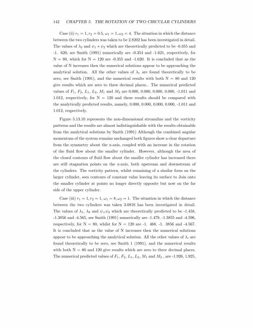
142 CHAPTER 5. THE ROTATION OF TWO CIRCULAR CYLINDERS
Case (ii) r1 = 1, r2 = 0.5, ω1 = 1, ω2 = 4. The situation in which the distance
between the two cylinders was taken to be 2.8202 has been investigated in detail.
The values of λ2 and ψ1 +ψ2 which are theoretically predicted to be -0.355 and
-1. 620, see Smith (1991) numerically are -0.354 and -1.621, respectively, for
N = 80, which for N = 120 are -0.355 and -1.620. It is concluded that as the
value of N increases then the numerical solutions appear to be approaching the
analytical solution. All the other values of λ1 are found theoretically to be
zero, see Smith (1991), and the numerical results with both N = 80 and 120
give results which are zero to three decimal places.. The numerical predicted
values of F1, F2, L1, L2, M1 and M2 are 0.000, 0.000, 0.000, 0.000, -1.011 and
1.012, respectively, for N = 120 and these results should be compared with
the analytically predicted results, namely, 0.000, 0.000, 0.000, 0.000, -1.011 and
1.012, respectively.
Figure 5.13.10 represents the non-dimensional streamline and the vorticity
patterns and the results are almost indistinguishable with the results obtainable
from the analytical solutions by Smith (1991) Although the combined angular
momentum of the system remains unchanged both figures show a clear departure
from the symmetry about the x-axis, coupled with an increase in the rotation
of the fluid flow about the smaller cylinder. However, although the area of
the closed contours of fluid flow about the smaller cylinder has increased there
are still stagnation points on the x-axis, both upstream and downstream of
the cylinders. The vorticity pattern, whilst remaining of a similar form on the
larger cylinder, sees contours of constant value leaving its surface to Join onto
the smaller cylinder at points no longer directly opposite but now on the far
side of the upper cylinder.
Case (iii) r1 = 1, r2 = 1, ω1 = 8, ω2 = 1. The situation in which the distance
between the two cylinders was taken 3.0816 has been investigated in detail.
The values of λ1, λ9 and ψ+ψ2 which are theoretically predicted to be -1.458,
-1.3856 and -4.565, see Smith (1991) numerically are -1.479, -1.3855 and -4.596,
respectively, for N = 80, whilst for N = 120 are -1. 468, -1. 3856 and -4.567.
It is concluded that as the value of N increases then the numerical solutions
appear to be approaching the analytical solution. All the other values of λi are
found theoretically to be zero, see Smith 1 (1991), and the numerical results
with both N = 80 and 120 give results which are zero to three decimal places.
The numerical predicted values of F1, F2, L1, L2, M1 and M2 , are -1.926, 1.925,
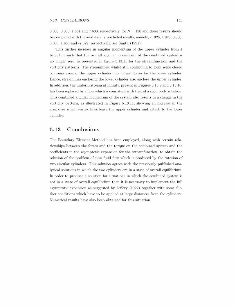
5.13. CONCLUSIONS 143
0.000, 0.000, 1.684 and 7.630, respectively, for N = 120 and these results should
be compared with the analytically predicted results, namely, -1.925, 1.925, 0.000,
0.000, 1.683 and -7.629, respectively, see Smith (1991).
This further increase in angular momentum of the upper cylinder from 4
to 8, but such that the overall angular momentum of the combined system is
no longer zero, is presented in figure 5.13.11 for the streamfunction and the
vorticity patterns. The streamlines, whilst still continuing to form some closed
contours around the upper cylinder, no longer do so for the lower cylinder.
Hence, streamlines enclosing the lower cylinder also enclose the upper cylinder.
In addition, the uniform stream at infinity, present in Figures 5.13.9 and 5.13.10,
has been replaced by a flow which is consistent with that of a rigid body rotation.
This combined angular momentum of the system also results in a change in the
vorticity pattern, as illustrated in Figure 5.13.11, showing an increase in the
area over which vortex lines leave the upper cylinder and attach to the lower
cylinder.
5.13 Conclusions
The Boundary Element Method has been employed, along with certain rela-
tionships between the forces and the torque on the combined system and the
coefficients in the asymptotic expansion for the streamfunction, to obtain the
solution of the problem of slow fluid flow which is produced by the rotation of
two circular cylinders. This solution agrees with the previously published ana-
lytical solutions in which the two cylinders are in a state of overall equilibrium.
In order to produce a solution for situations in which the combined system is
not in a state of overall equilibrium then it is necessary to implement the full
asymptotic expansion as suggested by Jeffery (1922) together with some fur-
ther conditions which have to be applied at large distances from the cylinders.
Numerical results have also been obtained for this situation.
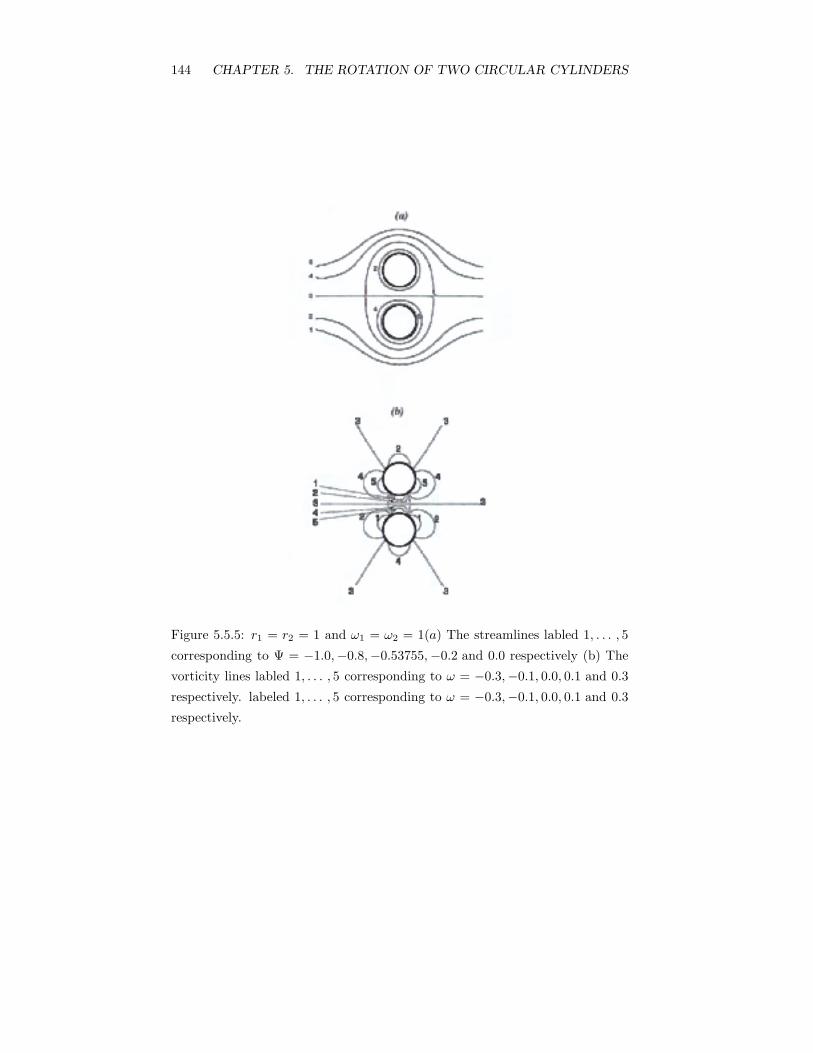
144 CHAPTER 5. THE ROTATION OF TWO CIRCULAR CYLINDERS
Figure 5.5.5: r1 = r2 = 1 and ω1 = ω2 = 1(a) The streamlines labled 1, . . . , 5
corresponding to Ψ = −1.0,−0.8,−0.53755,−0.2 and 0.0 respectively (b) The
vorticity lines labled 1, . . . , 5 corresponding to ω = −0.3,−0.1, 0.0, 0.1 and 0.3
respectively. labeled 1, . . . , 5 corresponding to ω = −0.3,−0.1, 0.0, 0.1 and 0.3
respectively.
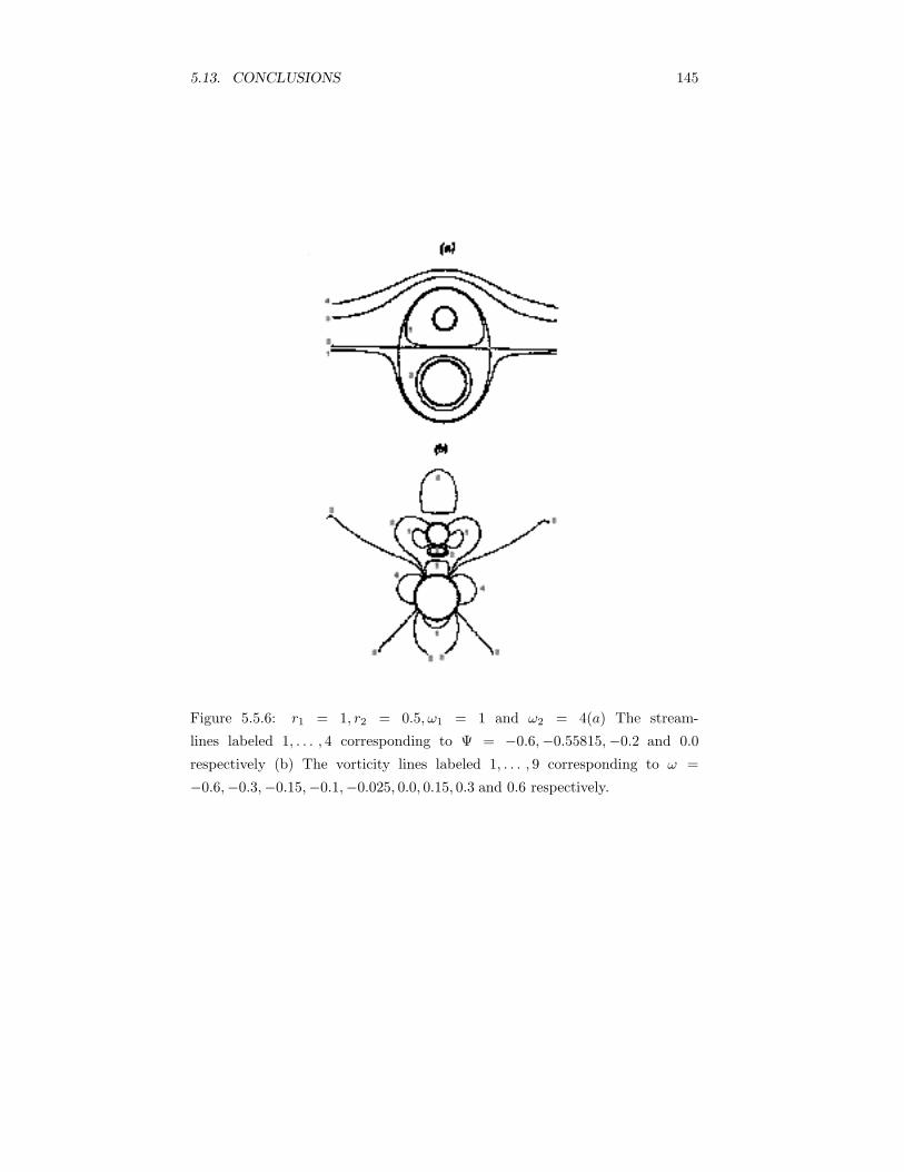
5.13. CONCLUSIONS 145
Figure 5.5.6: r1 = 1, r2 = 0.5, ω1 = 1 and ω2 = 4(a) The stream-
lines labeled 1, . . . , 4 corresponding to Ψ = −0.6,−0.55815,−0.2 and 0.0
respectively (b) The vorticity lines labeled 1, . . . , 9 corresponding to ω =
−0.6,−0.3,−0.15,−0.1,−0.025, 0.0, 0.15, 0.3 and 0.6 respectively.
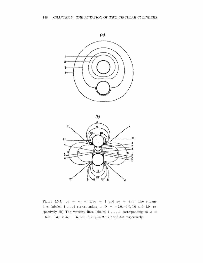
146 CHAPTER 5. THE ROTATION OF TWO CIRCULAR CYLINDERS
Figure 5.5.7: r1 = r2 = 1, ω1 = 1 and ω2 = 8.(a) The stream-
lines labeled 1, . . . , 4 corresponding to Ψ = −2.0,−1.0, 0.0 and 4.0, re-
spectively (b) The vorticity lines labeled 1, . . . , 11 corresponding to ω =
−6.0,−0.3,−2.25,−1.95, 1.5, 1.8, 2.1, 2.4, 2.5, 2.7 and 3.0, respectively.
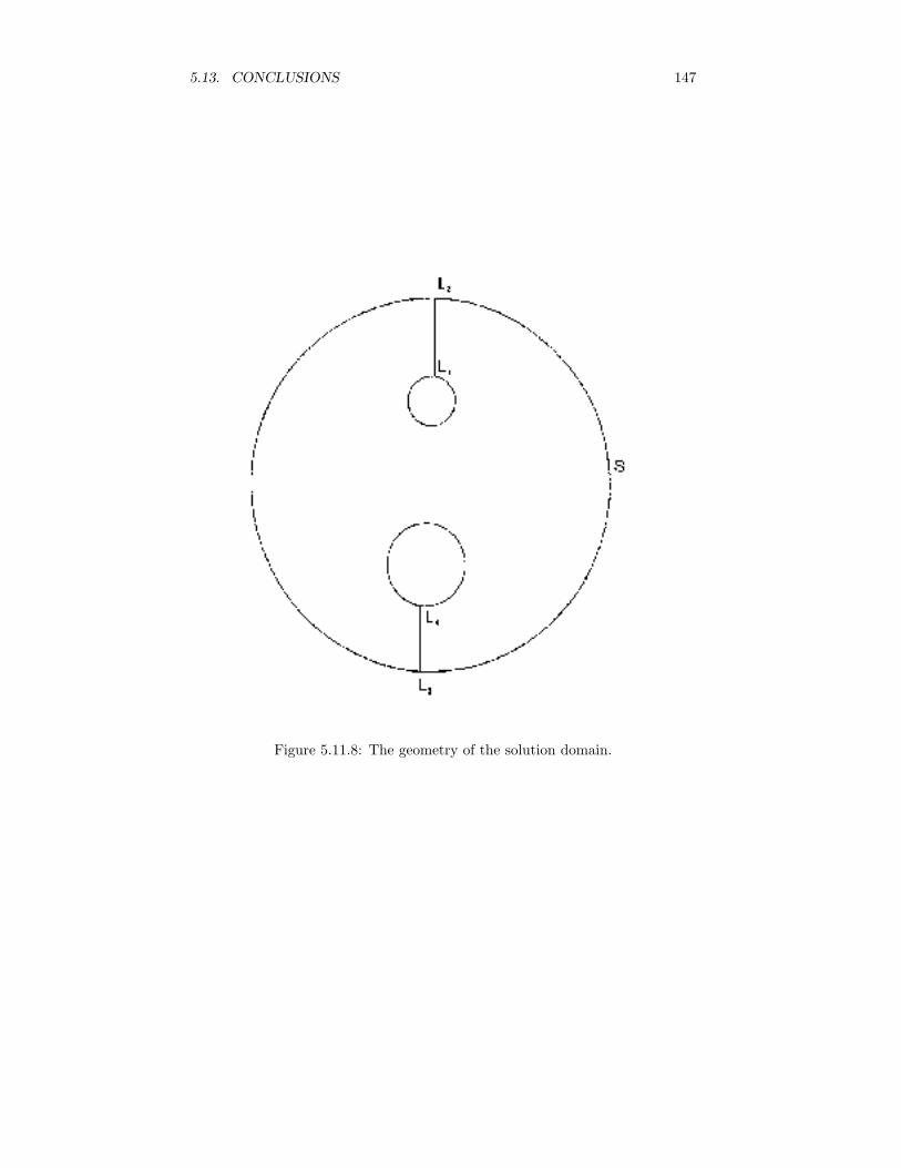
5.13. CONCLUSIONS 147
Figure 5.11.8: The geometry of the solution domain.
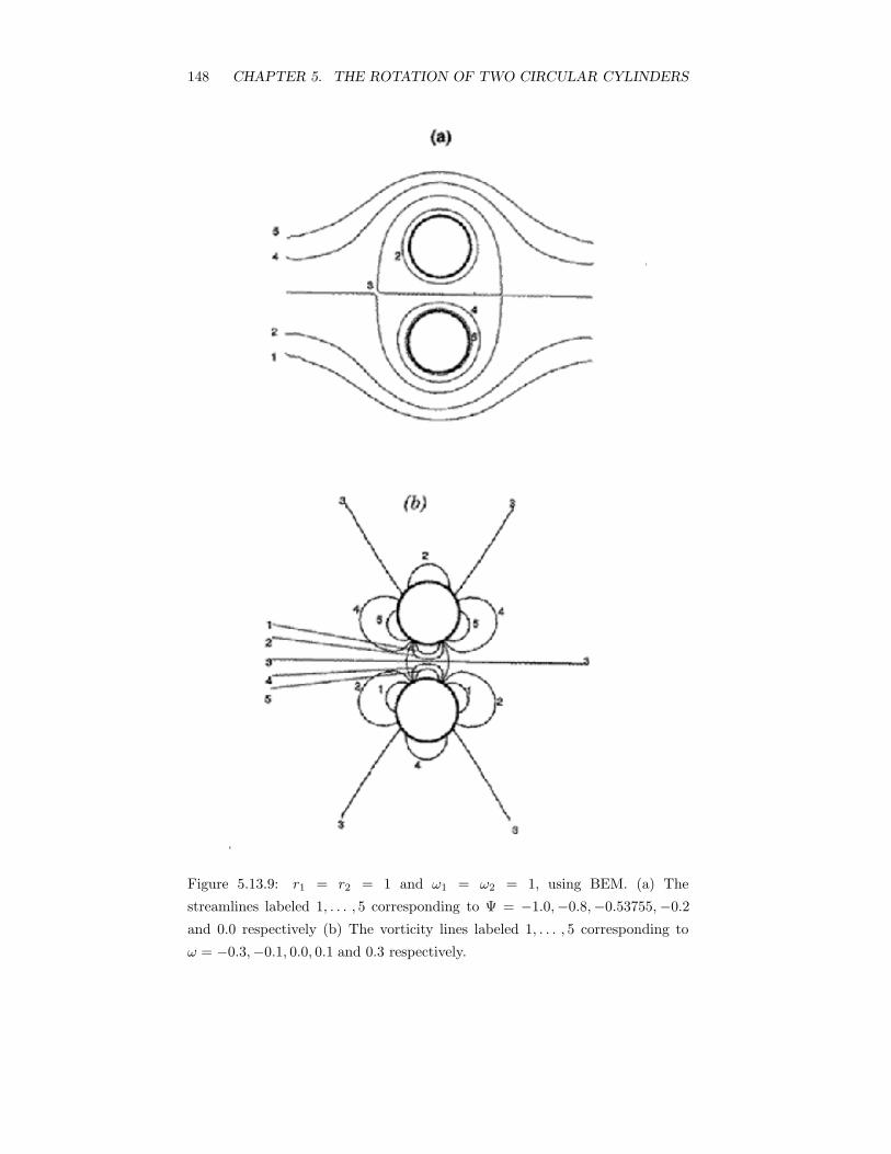
148 CHAPTER 5. THE ROTATION OF TWO CIRCULAR CYLINDERS
Figure 5.13.9: r1 = r2 = 1 and ω1 = ω2 = 1, using BEM. (a) The
streamlines labeled 1, . . . , 5 corresponding to Ψ = −1.0,−0.8,−0.53755,−0.2
and 0.0 respectively (b) The vorticity lines labeled 1, . . . , 5 corresponding to
ω = −0.3,−0.1, 0.0, 0.1 and 0.3 respectively.
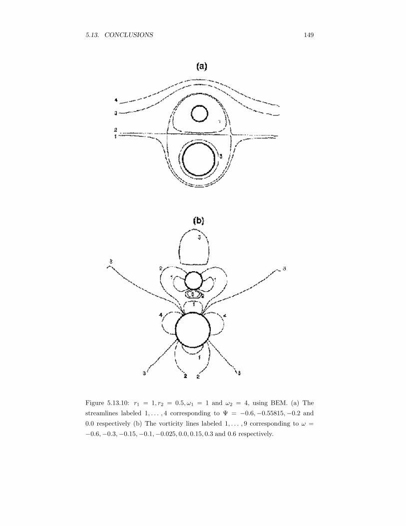
5.13. CONCLUSIONS 149
Figure 5.13.10: r1 = 1, r2 = 0.5, ω1 = 1 and ω2 = 4, using BEM. (a) The
streamlines labeled 1, . . . , 4 corresponding to Ψ = −0.6,−0.55815,−0.2 and
0.0 respectively (b) The vorticity lines labeled 1, . . . , 9 corresponding to ω =
−0.6,−0.3,−0.15,−0.1,−0.025, 0.0, 0.15, 0.3 and 0.6 respectively.
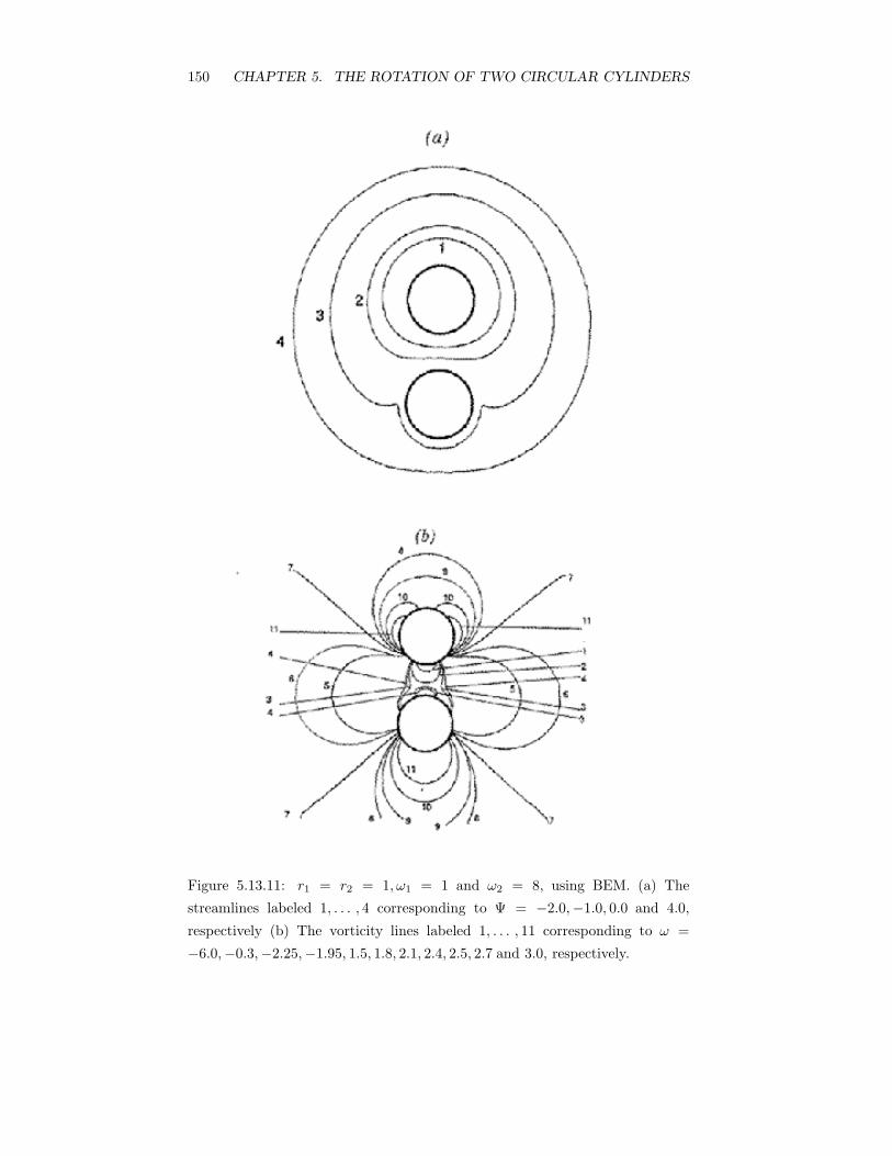
150 CHAPTER 5. THE ROTATION OF TWO CIRCULAR CYLINDERS
Figure 5.13.11: r1 = r2 = 1, ω1 = 1 and ω2 = 8, using BEM. (a) The
streamlines labeled 1, . . . , 4 corresponding to Ψ = −2.0,−1.0, 0.0 and 4.0,
respectively (b) The vorticity lines labeled 1, . . . , 11 corresponding to ω =
−6.0,−0.3,−2.25,−1.95, 1.5, 1.8, 2.1, 2.4, 2.5, 2.7 and 3.0, respectively.
Chapter 6
ELLIPTICAL CYLINDER
AND A ROTLET
6.1 Introduction
There are a good many known solutions of problems of the two-dimensional
motion of an infinite viscous fluid disturb by a moving solid body. [77] involves,
in the case of the elliptic cylinder, infinite vorticity and indeterminate velocities
at the ends of the axes.
In [72], first treat the problem as a limiting case of the motion of an ellipsoid
through infinite viscous fluid, and his solution fulfills all the boundary condi-
tions, in particular making the velocity zero at infinity, gives, in the limiting case
of the elliptic cylinder, a solution which involves the velocity being logarithmi-
cally infinite in the direction of flow. The solution appear to be unique, subject
to this condition, and has been obtained a definite value for the resistance and
then treated the circular cylinder as a limiting case of the elliptic cylinder.
The problem of slow viscous flow past elliptical cylinder in the presence of
rotlet has been solved analytically in [69], namely that of a rotlet of strength Γ
placed at a distance C, where
C = a cosh(γ), γ > α (6.1.1)
from a cylinder whose boundary is ξ = α, the transformation from Cartesian to
151
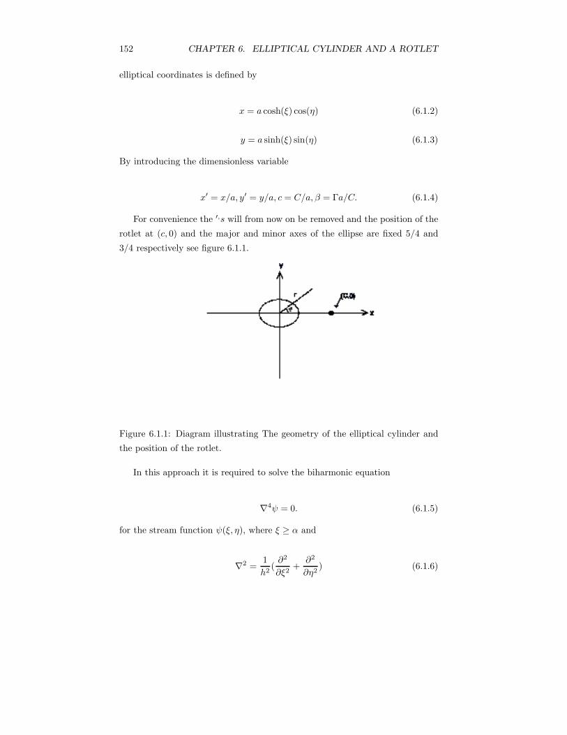
152 CHAPTER 6. ELLIPTICAL CYLINDER AND A ROTLET
elliptical coordinates is defined by
x = a cosh(ξ) cos(η) (6.1.2)
y = a sinh(ξ) sin(η) (6.1.3)
By introducing the dimensionless variable
x′ = x/a, y′ = y/a, c = C/a, β = Γa/C. (6.1.4)
For convenience the ′,s will from now on be removed and the position of the
rotlet at (c, 0) and the major and minor axes of the ellipse are fixed 5/4 and
3/4 respectively see figure 6.1.1.
Figure 6.1.1: Diagram illustrating The geometry of the elliptical cylinder and
the position of the rotlet.
In this approach it is required to solve the biharmonic equation
∇4ψ = 0. (6.1.5)
for the stream function ψ(ξ, η), where ξ ≥ α and
∇2 =1h2
(∂2
∂ξ2+
∂2
∂η2) (6.1.6)
6.1. INTRODUCTION 153
where
h = (cosh2(ξ) sin2(η) + sinh2(ξ) cos2(η))1/2 (6.1.7)
(ξ, η) are elliptic coordinates.
Before embarking on a numerical solution of this problem, it is important
to discuss the analytical solution obtained by [69] who found the Fourier Series
representation for the rotlet term
ψ0 =12
ln((x− c)2 + y2) (6.1.8)
to be given by
ψ0 = −∞∑
n=1
e−nγ
n(e−nξ + enξ) cos(η) + (ξ0 − ln(2))forξ < ξ0. (6.1.9)
He then put the complete solution as ψ = ψ0+ψ1where ψ1is the analytic out-
side the ellipse. Using the general solution of ∇4ψ = 0 as φ0 +(x2 +y2)φ1where
φ0and φ1are harmonic, we can write
ψ1 =12C0 + d0r
2 +∞∑
n=1
(Cne−nξ + 2dn(sinh(2ξ) + cos(2η)e−nξ) cos(nη)
(6.1.10)
The solution of ∇4ψ = 0 can be found by adding the general Fourier Series
in term of cos(nη) and sin(nη) to ψ0(ξ, η), which is the solution for the rotlet
in the absence of the ellipse, finding the coefficients in (6.1.10) to satisfy the
no-slip conditions, and the summing the series, i.e.
154 CHAPTER 6. ELLIPTICAL CYLINDER AND A ROTLET
ψ =12
ln[(cosh(ξ) cos η − cosh(γ) cosφ)2 + (sinh(ξ) sin η − sinh(γ) sinφ)2]
− 12
ln[(cosh(α) cos η − cosh(ξ + γ − α) cos φ)2 + (sinh(α) sin η
− sinh(ξ + γ − α) sinφ)2] + (ξ − α)
+ sinh(ξ − α) sin(η)Im[sinh(ξ + δ − γ)
sinh(δ)(cosh(ξ + δ − 2γ) − cos(η)
+ sinh(ξ − α)Re[cosh(ξ + α)e−δ
sinh(δ)cosh(2α)− cosh(α) − cosh(ξ + δ − α)cos(η)sinh(δ)(cosh(ξ + δ − 2γ) − cos(η)
]
(6.1.11)
where
δ = α − iφ, i =√−1, Imand Reare the imaginary and real parts in (6.1.11)
respectively. At large distances from the ellipse (6.1.11) can be written in the
form
ψ � Ar2 (6.1.12)
where
A =cos(2φ) − e−2γ
cosh(2α)[cosh(2γ) − cos(2φ)](6.1.13)
Hence a solid body rotation is induced at large distances from the ellipse except
at φ = arccos(e−2γ)/2 which give a uniform flow when a rotlet at this point see
figure 6.1.2. In fact, it is possible to obtain uniform flow at large distances of the
rotlet is placed at any one of four points due to symmetry of the problem. To
simplify the analytical solution in order to compare with the numerical solution
we put the analytical solution in the form
Ψ = ψB + ψ∗ (6.1.14)
where
6.1. INTRODUCTION 155
ψB = b1r cos(ϑ) + b2r sin(ϑ) + b3 + b4 sin(2ϑ) + b5 cos(2ϑ)
+ b6 ln(r) + b7r2 + b8r ln(r) cos(ϑ) + b9r ln(r) sin(ϑ)
+ ln(r2 + c2 − 2rc cos(ϑ)) + b10 cos(ϑ)/r + b11 sin(ϑ)/r
+ b12 cos(3ϑ)/r + b13 sin(3ϑ)/r
(6.1.15)
Figure 6.1.2: The uniform flow obtained when a rotlet at the position
(2.236,0.758).
The streamlines labeled 1, 2, 3, 4 and 5, correspond to
Ψ = −1.0, −0.5, 0.0, 0.5 and 1.0, respectively.
and ψB is the asymptotic expansion of ψ and ψ∗ is the perturbation value
about this expansion that tend to zero as r → ∞, if then we use sufficient large
r, say, r ≥ 30 and we use (6.1.11) to find the value of ψ and we repeat this 13
156 CHAPTER 6. ELLIPTICAL CYLINDER AND A ROTLET
times we can get 13 equations and 13 unknowns bj, j = 1, 2, . . . , 13 and we use
the Gauss required elimination method we can find the values of bj as
b1 = 0.500, b2 = 0.000, b3 = −1.092, b4 = 0.000, b5 = 0.208,
b6 = 0.000, b7 = 0.056, b8 = 0.000, b9 = 0.000, b10 = −0.015,
b11 = −2.585, b12 = 0.105, b13 = −0.002.
(6.1.16)
Equation (6.1.11) can be transform to the solution obtained by [16] by change
the variables by writing ξ + α in place of ξ, then the ellipse itself is given by
ξ = 0 and making α → ∞, a → 0, so that acoshα → A, asinhα → A, where A
is the radius of the cylinder see [72].
6.2 Forces and Moment on the Ellipse
The components of the force (Fx, Fy) and the moment M acting on a volume
V of fluid which is enclosed by the surface S can be expressed as
Fx =∫
S
(σξξ∂x/∂ξ − σξη∂y/∂ξ)dS/h (6.2.1)
Fy =∫
S
(σξξ∂y/∂ξ + σξη∂x/∂ξ)dS/h (6.2.2)
M =∫
S
[(σξξ∂x/∂ξ − σξη∂y/∂ξ)y − (σξξ∂y/∂ξ + σξη∂x/∂ξ)x]dS/h, (6.2.3)
where x and y in elliptic co-ordinates defined in (6.1.2) and (6.1.3) respec-
tively, and
σξξ = −p+ 2μ(∂Vξ
∂ξ/h− Vη
∂(1/h)∂η
) (6.2.4)
σξη = σηξ = μ(∂
∂ξ
[Vη
h
]+
∂
∂η
[Vξ
h
]) (6.2.5)
h =(cosh2(ξ) sin2(η) + sinh2(ξ) cos2(η)
)1/2(6.2.6)
6.3. THE GOVERNING EQUATIONS 157
Inserting these values of σξξ, σξηinto expressions (6.2.1),(6.2.2) and (6.2.3)
and using the Stokes equations of motion, we obtain, after some simplifications,
Fx =∫
S
[∂ω
∂nsinh(α) sin(η) − ω cosh(α) sin(η)/h
]ds, (6.2.7)
Fy = −∫
S
[∂ω
∂ncosh(α) cos(η) − ω sinh(α) cos(η)/h
]ds, (6.2.8)
M =∫
S
[∂ω
∂n
{cosh2(α) cos2(η) + sinh2(α) sin2(η)
}/2 + ω sinh(α) cosh(α)/h
]ds
(6.2.9)
The integrals, which occur in equations (6.2.7), (6.2.8) and (6.2.9) are evaluated
numerically using Simpson’s rule.
6.3 The Governing Equations
For slow steady, two-dimensional flow of an incompressible Newtonian fluid the
Navier-Stokes and continuity equations reduce to
∇p = ∇2u, (6.3.1)
∇ · u = 0, (6.3.2)
where the Reynolds number is assumed to be so small. On introducing the
stream function, ψ say, such that ∂ψ/∂x = −vyand ∂ψ/∂y = vx, then ψ satisfies
the biharmonic equation, see [5],
∇4ψ = 0. (6.3.3)
On introducing the vorticity, ω, equation (6.3.3) may be written in the following
form
∇2ψ = ω, (6.3.4)
158 CHAPTER 6. ELLIPTICAL CYLINDER AND A ROTLET
∇2ω = 0. (6.3.5)
In order to solve the equations (6.3.4) and (6.3.5) in the domain Ω we use the
BEM. For any p = (x, y) ∈ Ω ∪ ∂Ω and q = (x0, y0) ∈ ∂Ω, let
f(p, q) = ln | p− q |, (6.3.6)
g(p, q) =| p− q |2 (ln | p− q | −1), (6.3.7)
where | p− q |= {(x−x0)2 +(y−y0)2}1/2. Applying Green’s second identity
we have
η(p)ψ(p) =∫
∂Ω
ψ(q)f ′(p, q)dq −∫
∂Ω
ψ′(q)f(p, q)dq
+14
∫∂Ω
ω(q)g′(p, q)dq − 14
∫∂Ω
ω′(q)g(p, q)dq(6.3.8)
η(p)ω(p) =∫
∂Ω
ω(q)f ′(p, q)dq −∫
∂Ω
ω′(q)f(p, q)dq (6.3.9)
The boundary is first calculated by using Runge Kitta method and is found
6.386 which is agree with handbook of mathematical table and then subdivided
into N segments, ∂Ωj , by solving differential equation
dη/ds = 1/h (6.3.10)
and the stream function, ψ, its derivative, ψ′, the vorticity, ω, and its deriva-
tive, ω′, are approximated by piecewise constant functions. This results in the
following system of algebraic equations
∑Nj=1 Eijψj −Gijψ
′j + Lijωj −Mijω
′j = 0∑N
j=1 Eijωj −Gijω′j = 0
}i = 1, . . . , n (6.3.11)
where Gij , Eij , Lij and Mij are given by
Gij =∫
∂Ωj
f(pi, q)dq,
6.4. NUMERICAL SOLUTION 159
Eij =∫
∂Ωj
f ′(pi, q)dq − η(pi)δij ,
Lij =14
∫∂Ωj
g′(pi, q)dq,
Mij =14
∫∂Ωj
g(pi, q)dq,
Equations (6.3.11) represents 2N equations in 4N unknowns. With the
application of the appropriate conditions the system of equations (6.3.11) can
be solved and equations (6.3.8) and (6.3.9) used to find the value of the stream
function, ψ, at any point within the solution domain, Ω.
6.4 Numerical Solution
In the present work the fluid flow passing through an elliptical cylinder in the
presence of a rotlet is investigated. In the mathematical model the fluid flow is
assumed to be two-dimensional and the ellipse, with major and minor axes of
lengths a and b, respectively, and the rotlet is at a distance c from the center of
the ellipse as shown in figure (6.1.1).
In order to solve numerically Navier-Stokes equations in an exterior region,
it is very advantageous to use the BEM because there is a simple fundamental
solution, which enables one to covert the equations into integral equations, which
only involves boundary integrals. Further, these integral equations are very
convenient when dealing with the infinite boundary condition, see for example
[41] and [9].
In this work the BEM with constant elements is used. It is convenient to
separate the stream function and the vorticity into two parts, namely,
Ψ = ψA + ψ∗ (6.4.1)
ω = ωA + ω∗ (6.4.2)
where
160 CHAPTER 6. ELLIPTICAL CYLINDER AND A ROTLET
ψA = λ1r cos(ϑ) + λ2r sin(ϑ) + λ3 + λ4 sin(2ϑ)
+ λ5 cos(2ϑ) + λ6 ln(r) + λ7r2 + λ8r ln(r) cos(ϑ)
+ λ9r ln(r) sin(ϑ) + (β/2) ln(r2 + c2 − 2rc cos(ϑ))
(6.4.3)
ωA = −4λ4 sin(2ϑ)/r2 − 4λ5 cos(2ϑ)/r2 − 47λ
− 2λ8 cos(ϑ)/r − 2λ9 sin(ϑ)/r(6.4.4)
Those ψA and ωA are asymptotic expansions of ψ and ω as r → ∞, and ψ∗
and ω∗ are the perturbations values about these expansions that tend to zero
as r → ∞,
Considering the surface of the ellipse as the streamline ψ = 0, then ψ∗ and
ω∗ satisfies
∇2ψ∗ = ω∗ (6.4.5)
∇2ω∗ = 0. (6.4.6)
with
ψ∗ = −ψA and ψ∗′ = −ψ′A on the boundary (6.4.7)
Equations (6.4.7) provides another N equations to be 2N and the number
of unknowns 2N + 9 which means that we need another 9 conditions to close
the system
The extra unknowns λj , where j = 1, . . . , 9, will require extra conditions:
Case (a)
Let us assume for the moment that the values of the drag, lift and moment
are all zeros. Using the expressions (6.2.7), (6.2.8) and (6.2.9) where we have
replaced ω by ωA + ω∗, the parts of the integrals involving ωA were evaluated
analytically producing linear expressions in the unknowns λj . The other parts
involving ω∗ are expressed after numerical integrations using Simpson’s method
as linear expressions in ω∗j and ω∗′
j . The resulting expressions for the drag, lift
and moment can be written as
6.4. NUMERICAL SOLUTION 161
(N−1)/2∑j=1
[(ω∗′2j−1 + 4ω∗′
2j + ω∗′2j+1) sinh(α) sin(ηj)
− (ω∗2j−1 + 4ω∗
2j + ω∗2j+1) cosh(α) sin(ηj)/hj ](2π/3N ) = 0,
(6.4.8)
(N−1)/2∑j=1
[(ω∗′2j−1 + 4ω∗′
2j + ω∗′2j+1) cosh(α) cos(ηj)
− (ω∗2j−1 + 4ω∗
2j + ω∗2j+1) sinh(α) cos(ηj)/hj ](2π/3N ) = 0,
(6.4.9)
(N−1)/2∑j=1
[(ω∗′2j−1 + 4ω∗′
2j + ω∗′2j+1)h
2j/2
+ (ω∗2j−1 + 4ω∗
2j + ω∗2j+1) sinh(α)coh(α)/hj ](2π/3N ) = 0,
(6.4.10)
where
hj = (cosh2(α) sin2(ηj) + sinh2(α) cos2(ηj))1/2 (6.4.11)
ω∗1 = ω∗
N , (6.4.12)
ω∗′1 = ω∗′
N , (6.4.13)
Equations (6.4.8), (6.4.9) and (6.4.10) gives three conditions plus one extra
condition arising from the fact that the pressure distribution is single value(6.4.14).
−(N−1)/2∑
j=1
[(ω∗′2j−1 + 4ω∗′
2j + ω∗′2j+1)](2π/3N ) = 0 (6.4.14)
Hence, equations (6.4.5) and (6.4.6), together with (6.4.8), (6.4.9), (6.4.10)
and (6.4.14) result in (2N+4) equations in terms of the (2N+9) unknowns which
mean that we need five extra conditions to complete the system of equations.
In order to obtain the other equations, we make use of the fact that η(p)
vanishes outside the domain, i.e when p is inside the elliptical cylinder, namely
p(ξIj , ηj), where ξIj < α for j = 1, 2, 3, 4 and 5
162 CHAPTER 6. ELLIPTICAL CYLINDER AND A ROTLET
Case (b)
In this situation we use the asymptotic expansion of ψ given in equation
(6.4.3). Hence, equations (6.4.8), (6.4.9) and (6.4.10) have to be replace by
− 4πλ9 +(N−1)/2∑
j=1
[(ω∗′2j−1 + 4ω∗′
2j + ω∗′2j+1) sinh(α) sin(ηj)
− (ω∗2j−1 + 4ω∗
2j + ω∗2j+1) cosh(α) sin(ηj)/hj ](2π/3N ) = 0,
(6.4.15)
4πλ8 −(N−1)/2∑
j=1
[(ω∗′2j−1 + 4ω∗′
2j + ω∗′2j+1) cosh(α) cos(ηj)
− (ω∗2j−1 + 4ω∗
2j + ω∗2j+1) sinh(α) cos(ηj)/hj ](2π/3N ) = 0,
(6.4.16)
4πλ6 −(N−1)/2∑
j=1
[(ω∗′2j−1 + 4ω∗′
2j + ω∗′2j+1)h
2j/2
+ (ω∗2j−1 + 4ω∗
2j + ω∗2j+1) sinh(α)coh(α)/hj ](2π/3N ) = 0
(6.4.17)
Then we can proceed in the same way as described in case (a). However
in this situation we did not assume that the forces and the moment are zero.
This hover has given rise to certain computational difficulties, which we will
discuss in some detail later in the results section. To overcome these difficulties
we developed case (c):
Case (c)
Here we used the same methodology adapted in case (b) except that we have
replaced the lift condition (6.4.16) by one point inside the ellipse. This gave us
six points inside the ellipse, one integral condition (6.4.14) together with the
expressions for the drag (6.4.15) and that for the moment (6.4.17).
6.5 Numerical Results
Numerical details for situations when the position of the rotlet at (2.236,0) is
presented for three cases
Initially case (a) the drag, the lift and the moment are all enforce to be zero.
The values of λ1, λ2, λ3, λ4, λ5, λ6, λ7, λ8 and λ9 which are analytically are
6.6. CONCLUSIONS 163
0.500, 0.000, −1.092, 0.000, 0.208, 0.000, 0.056, 0.000 and 0.000 numerically
are 0.477, 0.000, −1.091, −0.024, 0.204, 0.000, 0.056, 0.032 and 0.006 respec-
tively. The above inaccuracies arising in the coefficients are overcome by using
case (c).
In case (b) The asymptotic expansion for the drag, the lift and the moment
at infinity are included. The values of λ1, λ2, λ3, λ4, λ5, λ6, λ7, λ8
and λ9 are 0.477, 0.000, −1.091, −0.024, 0.204, 0.000, 0.056, 0.032 and 0.006
respectively which are also inaccurate as in case (a).
In case (c) six points inside the elliptical cylinder were used beside the
asymptotic expansion at infinity of the drag and the moment and the inte-
gral condition, this case was chosen because the lift is appear to be inac-
curate in case (b) and is very sensitive to the discretization. The values of
λ1, λ2, λ3, λ4, λ5, λ6, λ7, λ8 and λ9 for N = 600 are 0.501, 0.000, -1.091,
0.001, 0.207, 0.000, 0.056, 0.000 and 0.000 respectively
Figure 6.5.1 represents the non-dimensional streamline pattern and the vor-
ticity pattern. The streamline is symmetric about the x-axis and show a rota-
tional flow about the elliptical cylinder and form closed contours a round the
cylinder and the rotlet, together with a stagnation point on the x-axis opposite
to the position of the rotlet. However, due to the different values of c the po-
sition of stagnation points differ. The streamline for −0.65, 0.00 and 0.19 are
presented also the non-dimensional vorticity for −0.07, 0.0, 0.22, 0.3 and 0.4
are presented in figure 6.5.1(b).
Figure 6.5.2 represents the non-dimensional streamline pattern and the vor-
ticity pattern. The streamline is symmetric about the y-axis and show a rota-
tional flow about the elliptical cylinder and form closed contours a round the
cylinder and the rotlet, together with a stagnation point on the y-axis. How-
ever, due to the different values of c the position of stagnation points differ.
The streamline for −1.5, −0.75, 0.0, 0.75 and 1.5 are presented also the non-
dimensional vorticity for −0.5, −0.4, 0.0 and 0.2 are presented in figure 6.5.2(b).
6.6 Conclusions
The numerical technique used in chapters 4 and 5 have again been employed
in order to investigate the slow viscous flow past an elliptical cylinder in the
164 CHAPTER 6. ELLIPTICAL CYLINDER AND A ROTLET
presence of a rotlet. It is found that the numerical results are in reasonable
agreement with those obtained analytically.
It is found that the determination of the lift is very sensitive to the form of
the discretization. In order to overcome this problem it was found necessary to
use six points inside the elliptical cylinder, instead of the expected five points,
with the constraint on the lift being omitted.
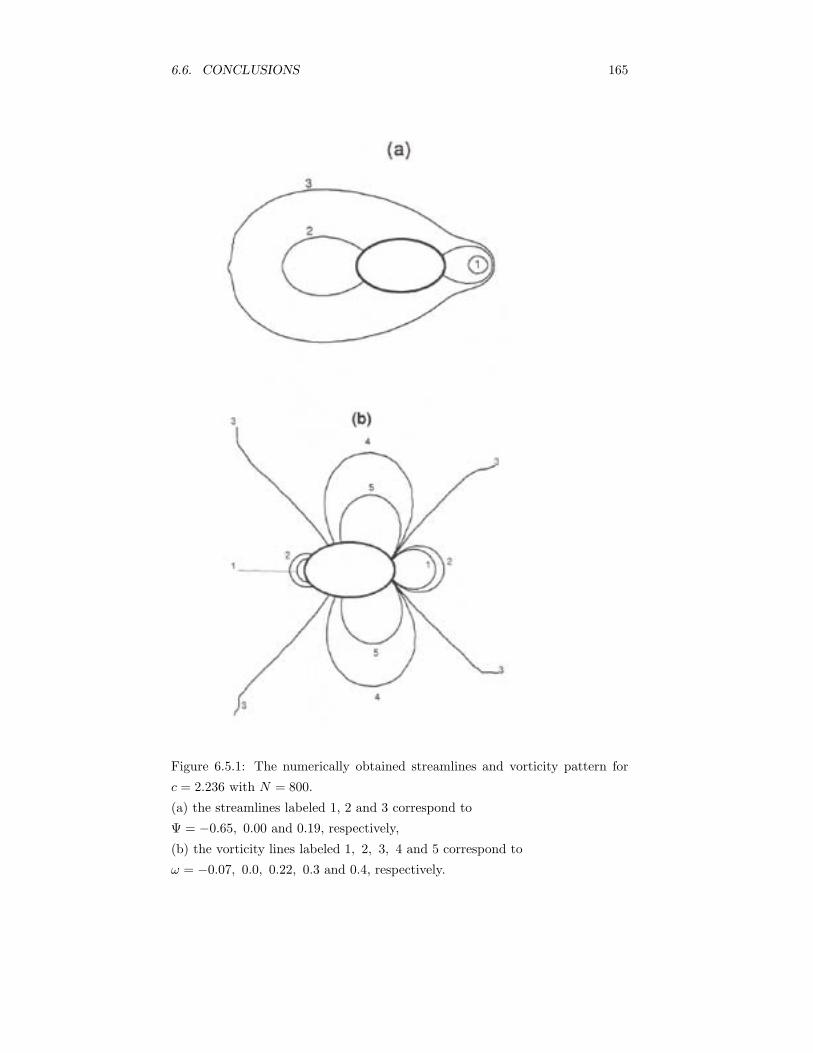
6.6. CONCLUSIONS 165
Figure 6.5.1: The numerically obtained streamlines and vorticity pattern for
c = 2.236 with N = 800.
(a) the streamlines labeled 1, 2 and 3 correspond to
Ψ = −0.65, 0.00 and 0.19, respectively,
(b) the vorticity lines labeled 1, 2, 3, 4 and 5 correspond to
ω = −0.07, 0.0, 0.22, 0.3 and 0.4, respectively.
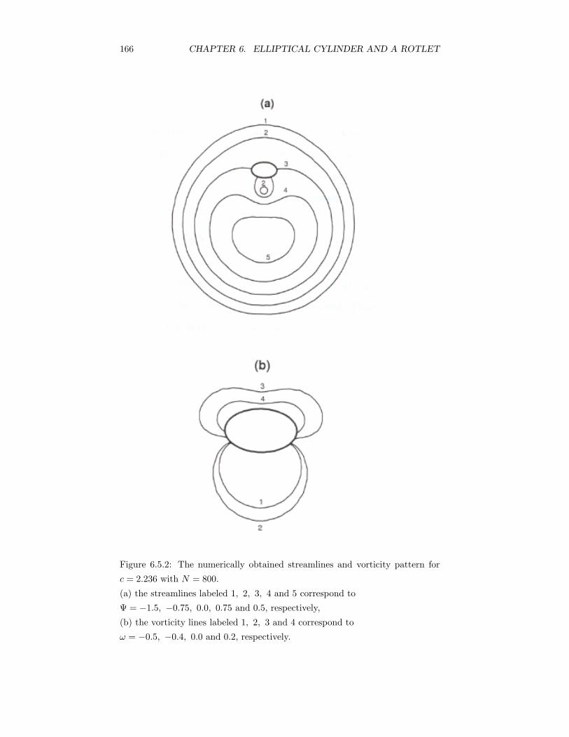
166 CHAPTER 6. ELLIPTICAL CYLINDER AND A ROTLET
Figure 6.5.2: The numerically obtained streamlines and vorticity pattern for
c = 2.236 with N = 800.
(a) the streamlines labeled 1, 2, 3, 4 and 5 correspond to
Ψ = −1.5, −0.75, 0.0, 0.75 and 0.5, respectively,
(b) the vorticity lines labeled 1, 2, 3 and 4 correspond to
ω = −0.5, −0.4, 0.0 and 0.2, respectively.
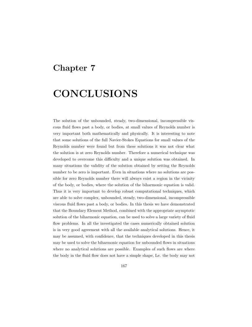
Chapter 7
CONCLUSIONS
The solution of the unbounded, steady, two-dimensional, incompressible vis-
cous fluid flows past a body, or bodies, at small values of Reynolds number is
very important both mathematically and physically. It is interesting to note
that some solutions of the full Navier-Stokes Equations for small values of the
Reynolds number were found but from these solutions it was not clear what
the solution is at zero Reynolds number. Therefore a numerical technique was
developed to overcome this difficulty and a unique solution was obtained. In
many situations the validity of the solution obtained by setting the Reynolds
number to be zero is important. Even in situations where no solutions are pos-
sible for zero Reynolds number there will always exist a region in the vicinity
of the body, or bodies, where the solution of the biharmonic equation is valid.
Thus it is very important to develop robust computational techniques, which
are able to solve complex, unbounded, steady, two-dimensional, incompressible
viscous fluid flows past a body, or bodies. In this thesis we have demonstrated
that the Boundary Element Method, combined with the appropriate asymptotic
solution of the biharmonic equation, can be used to solve a large variety of fluid
flow problems. In all the investigated the cases numerically obtained solution
is in very good agreement with all the available analytical solutions. Hence, it
may be assumed, with confidence, that the techniques developed in this thesis
may be used to solve the biharmonic equation for unbounded flows in situations
where no analytical solutions are possible. Examples of such flows are where
the body in the fluid flow does not have a simple shape, Le. the body may not
167
168 CHAPTER 7. CONCLUSIONS
be smooth or have a complex shape, and also where multiply bodies are present
in the flow. Future extensions of this work should address such flows.
Bibliography
[1] Alarcon, E., Martin, A. and Paris, F., 1979, Boundary Element in Poten-
tial and Elasticity Theory, Comp. and Stru., 10, 351 − 362.
[2] Badr, H.M. and Dennis, S.C.R., 1985, Time-dependent Viscous Flow Past
an Impulsively Started Rotating and Translating Circular Cylinder, J.
Fluid Mech. 158, 447 − 488.
[3] Backus, G. and Gilbert, F., 1970, Uniqueness in the Inversion of Inaccu-
rate Gross Earth Data, Phil. Trans R. Soc. London Ser. A266,123− 192.
[4] Banerjee, P.K., and Butterfield, R., 1981, Boundary Element Methods in
Engineering Science, Mcgraw-Hill, New York.
[5] Batchelor, G.K. (1967) An Introduction to Fluid Dynamics, Cambridge
University Press, London, New York, Melbourne.
[6] Beck, J.V., Blackwell, B. and St. Clair, C.R., 1985, Inverse Heat Conduc-
tion, Wiley-Interscience, London, Washington.
[7] Bialecki, R. and Nowak, A.J., 1981, Boundary Value Problem in Heat Con-
duction with Nonlinear Material and Boundary Conditions, Appl. Math.
Modelling. 5, 416 − 421.
[8] Brebbia, C.A. and Gipson, G.S. (Editor), 1991, Proc. 13th Int. Conf.
on Boundary Element Methods in Enginering, Springer-Verlag, Berling,
Heidelberg, New York, Tokyo.
[9] Brebbia, C.A., Telles, J.C.F. and Wrobel, L.C., 1984, Boundary Element
Techniques, Springer-Verlag, Berling, Heidelberg, New York and Tokyo.
169
170 BIBLIOGRAPHY
[10] Bretherton, F.P., 1961, The Motion of Long Bubbles in Tubes, J. Fluid
Mech., 10, 166 − 189.
[11] Carrera, J. and Neuman, S.P., 1986, Estimation of Aquifer Parameters
Under Transient and Steady State Conditions, Parts 1, 2 and 3, Water
Resources Research, 22, 199 − 242.
[12] Chen, W.H. and Seinfeld, J.H., 1972, Estimation of Spatially Varying
Parameters in Partial Differential Equations, Int. J. Control, 15, 487−495.
[13] Cox, B.G., 1962, On Driving a Viscous Fluid out of a Tube, J.Fluid Mech.,
14, 81− 96.
[14] Coyne, J.C. and Elrod, H.G., 1970, Conditions for the Rupture of a Lubri-
cating Film, Part 1, Theoretical Model, Trans. A.S.M.E. J. of Lub. Tech.,
92, 451 − 456.
[15] Dennis, S.C.R. and Chang, G.Z., 1970, Numerical Solution for Steady
Flow Past a Circular Cylinder at Reynolds Numbers up to 100, J. Fluid
Mech. 42, 471 − 489.
[16] Dorrepaal, J.M., O,Neill, M.E. and Ranger, K.B., 1984, Two-dimentional
Stokes Flows with Cylinders and Line Singularities, Mathematika 31, 65−75.
[17] Falk, R.S. and Monk, P.B., 1986, Logarithmic Convexity for Discrete
Harmonic Functions and the Approximation of the Cauchy Problem for
Poison,s Equations, Math. of Comp., 47, 135 − 149.
[18] Filon, L.N.G., 1926 The Forces on a Cylinder in a Stream of Viscous Fluid,
Proc. Roy. Soc., A113, 7 − 27.
[19] Fornberg, B., 1980, A Numerical Study of Steady Viscous Flow Past a
Circular Cylinder, J. Fluid Mech. 98, 819 − 855.
[20] Fornberg, B., 1985, Steady Viscous Flow Past a Circular Cylinder up to
Reynolds number 600, J.Comput. Phys. 161, 297 − 320.
[21] Fletcher, R., 1981, Practical Methods of Optimization, 2, Constrained
Optimization, John Wiley and Sons, New York and Toronto.
BIBLIOGRAPHY 171
[22] Flynn, M.R. and Ellenbecker, M.J., 1985, The Potential Flow Solution
for Air Flow into a Flanged Circular Hood, Am. Ind. Hyg. Assoc. J.,
46, 318 − 322.
[23] Flynn, M.R. and Miller, C.T., 1991, Discrete Vortex Methods for the
Simulation of Boundary Layer Separation Effects on Worker Exposure,
Ann. Occup. Hyg., 35, 35− 50.
[24] Fredholm, I., 1903, Sur Une Classe D,equations Fonctionells, Acta Math.,
27, 365 − 439.
[25] Gilbarg, D. and Trudinger, N.S., 1983, Elliptic Partial Differential Equa-
tions of Second Order, 2ndEd., Springer-Verlag, Berlin, Heidelberg, New
York, Tokyo.
[26] Guschchin, V.A. and Schennikov, V.V., 1974, A Numerical Method
of Solving the Navier-Stokes Equations, Zh. Vychist. Mat. Mat. Fiz.
14, 242 − 250.
[27] Gill, P.E., Murray, W. and Wright, M.H., 1981, Practical Optimization,
Academic Press, London and New York.
[28] Glauert, M.B., 1957 The Flow Past a Rapidly Rotating Circular Cylinder,
Proc. Roy. Soc. Lond. A242, 108 − 115.
[29] Glauert, M.B., 1957A Boundary Layer Theorem, with Applications to
Cylinders, J. Fluid Mech. 2, 89 − 99.
[30] Hamielec, A.E. and Raal, J.D., 1969 Numerical Studies of Viscous Flow
around Circular Cylinders, Phys. Fluids 12, 11 − 20.
[31] Han, H., 1982, The Finite Element Method in a Family of Improperly
Posed Problems, Math. of Comp., 38, 55 − 65.
[32] Homsy, G.M., 1987, Viscous Fingering in Porous Media, Annu. Rev. Fluid
Mech., 19, 271 − 311.
[33] Imai, I., 1951, On the Asympototic Behaviour of Viscous Fluid Flow at a
Great Distance from a Cylinderical Body, Proc. Roy. Soc. A208, 487−516.
172 BIBLIOGRAPHY
[34] Kelmanson, M.A., 1984, Boundary Integral Equation Analysis of Singu-
lar, Potential and Biharmonic Problems, 7, Lecture Notes in Engineering,
Springer-Verlag, Berlin, Heidelberg, New York, Tokyo.
[35] Tang, T., 1990, A Numerical Investigation into the Steady Flow Past a
Rotating Circular Cylinder at Low and Intermediate Reynolds Numbers,
J. Comput. Phys., 87, 91− 107.
[36] Harrington, R.F., Pontoppidan, K., Abrahamsen, P. and Albertsen,
N.C., 1969, Computation of Laplacian Potentials by an Equivalent-source
Method, Proc, IEE 116, 1715− 1720.
[37] Hess, J.L., and Smith, A.M.O., 1967, Calculation of Potential Flow about
Arbitrary Bodies, Progress in Aeronautical Sciences, 8, Pergamon Press,
London.
[38] Jeffery, G.B., 1920, Plane Stress and Plane Strain in Bipolar Co-ordinates,
Phil Trans., A221, 265 − 293.
[39] Jeffery, G.B., 1922, The Rotation of Two Circular Cylinders in a Viscous
Fluid, Proc. Roy. Soc. London Ser. A101, 169 − 174.
[40] Jaswon, M.A., 1963, Integral Equation Methods in Potential Theory, I,
Proc. Roy. Soc. Ser., A275, 23 − 32.
[41] Jaswon, M.A. and Symm, G.T., 1977, Integral Equation Methods in Po-
tential Theory and Elastostatics, Academic Press, London.
[42] Jain, P.C. and Kawakuti, M., 1966 Numerical Study of a Viscous Fluid
Past a Circular Cylinder, J. Phys. Soc. Japan 21, 2055 − 2062.
[43] Jain, P.C. and Sankara, Rao, K., 1969, Numerical Solution of Unsteady
Viscous Incompressible Fluid Flow Past a Circular Cylinder, Phys. Fluids
Suppl. II, 57 − 61.
[44] Kawaguti, M., 1953, Numerical Solution of the Navier-Stokes Equations
for the Flow Around a Circular Cylinder at Reynolds Number 40, J. Phys.
Soc. Japan 8, 747 − 757.
[45] Khader, M.S., 1980, Heat Conduction with Temperature Dependent Ther-
mal Conductivity, Paper 80 − HT − 4, National Heat Transfer Conf.,
ASME, Orlando, Florida.
BIBLIOGRAPHY 173
[46] Kuiken, H.K., 1990, Deforming Surface and Viscous Sintering, Proc. Conf.
on the Math. and the Comp. of Deforming Surface, Oxford Univ. Press,
London and New York.
[47] Lachat, J.C. and Watson, J.O., 1976, Effective Numerical Treatment of
BIE, Int. J. Num. Meth. in Eng., 10, 991 − 1005.
Langlois, W.E., 1964, Slow Viscous Flow, Macmillan, New York.
[48] Lavrentiev, M.M., 1956, On the Cauchy Problem for the Laplace Equa-
tion, Izv. Akad. Nauk SSSR Ser. Math., 20, 819 − 842(Russian).
[49] Louguet-Higgins, M.S. and Cokelet, E.D., 1976, The Deformation of Steep
Surface Waves on Water, Part, 1 A Numerical Method of Computation,
Proc. Roy. Soc. London, A350, 1 − 26.
[50] Lyul V.A., 1970 Numerical Solution of the Problem of the Rotation of
a Cylinder in a Flow of Viscous Incompressible Fluid, Zh. Vychisl. Mat.
Mat. Fiz., 17, 470 − 481.
[51] Manzoor, M., 1982, Heat Flow Through Extended Surface Heat Ex-
changes, Lecture Notes in Engineering, 5, Springer-Verlag, Berlin, Hei-
delberg, New York, Tokyo.
[52] Moore, D.W., 1957, The Flow Past a Rapidly Rotating Circular Cylinder
in an Infinite Stream, J. Fluid Mech. 2, 541 − 550.
[53] Nieuwstadt, F. and Keller, H.B., 1973 Viscous Flow Past Circular Cylin-
ders, Comp. Fluids 1, 59 − 71.
[54] Oberhettinger, F., 1973 Fourier Expansions, Academic Press, New York.
[55] Patel, V.A., 1981, Flow Around an Impulsively Started Elliptic Cylinder
at Various Angles of Attack, Comp. Fluids 9, 435 − 462.
[56] Payne, L.E., 1960, Bounds in the Cauchy Problem for the Laplace Equa-
tion, Arch. Rational Math. Anal., 5, 35 − 45.
[57] Payne, L.E., 1970, On a Priori Bounds in the Cauchy Problem for Elliptic
Equations, SIAM J. Math. Anal., 1, 82 − 89.
[58] Payne, L.E., 1975, Improperly Posed Problems in Partial Differential
Equations, Regional Conf. Ser. Appl. Math. Philagelphia, PA SIAM.
174 BIBLIOGRAPHY
[59] Prandtl, L. and Tietjens, O.G., 1934, Applied Hydro-mechanics and
Aeromechanics, McGraw-Hill, New York.
[60] Proudman, I. and Pearson, J.R.A., 1957, Expansions at Small Reynolds
Numbers for the Flow Past a Sphere and a Circular Cylinder, J. Fluid
Mech. 2, 237 − 262.
[61] Saffman, P.G., 1982, Lecture Notes in Physics, 154, Springer-Verlag,
Berlin, Heidelberg, New York, Tokyo.
[62] Shail, R. and Onslow, S.H., 1988, Some Stokes Flows Exterior to a Spher-
ical Boundary, Mathematika 35, 233 − 246.
[63] Shen, E.I. and Udell, K.S., 1985, A Finite Element Study of Low Reynolds
Number Two Phase Flow in Cylindrical Tubes, J. Appl. Mech., 52, 253−256.
[64] Sayers, A.T., 1979, Lift Coefficient and Flow Visualization on the Leading
Edge Rotating Cylinder Rudder, Int. J. Mech. Elec. Engng 7, 75 − 87.
[65] Smith, F.T., 1979 Laminar Flow of an Incompressible Fluid Past a Bluff
Body: the Separation, Reattachment, Eddy Properties and Drag, J. Fluid
Mech. 92, 171 − 205.
[66] Smith, F.T., 1985A Structure for Laminar Flow Past a Bluff Body at High
Reynolds Number, J. Fluid Mech. 155, 175 − 191.
[67] Smith, G.D., 1984, Numerical Solution of Partial Differential Equations:
Finite Difference Methods, 3rd.Ed., Oxford Applied Mathematics and
Computing Science Series.
[68] Smith, S.H., 1990, The Jeffery Paradox as the Limit of a Three-
dimentional Stokes Flow, Phys. Fluids A2(5), 661 − 673.
[69] Smith, S.H., 1991, The Rotation of Two Circular Cylinders in a Viscos
Fluid, Mathematika, 38, 63 − 66.
[70] Symm, G.T., 1963, Integral Equation Methods in Potential Theory, II,
Proc. Roy. Soc. Ser. A275, 33 − 46.
[71] Symm, G.T., 1973, Treatment of Singularities in the Solution of Laplace,s
Equation by an Integral Equation Method, NPL Report NCA31.
BIBLIOGRAPHY 175
[72] Swain, M., 1922, The Steady Motion of a Cylinder Through Infinite Vis-
cous fluid, Proc. Roy. Soc. Ser. A102, 766 − 778.
[73] Tennant, J.S., Johnson, W.S. and Krothapalli, A., 1976, Rotating Cylin-
der for Circulation Control on an Aerofoil, J. Hydronautics 10, 102− 117.
[74] Tuann, S.Y. and Olson, M.D., 1978, Numerical Studies of the Flow Around
a Circular Cylinder by a Finite Element Method, Comp. Fluids 6, 219 −240.
[75] Underwood, R.L., 1969, Calculations of Incompressible Flow Past a Circu-
lar Cylinder at Moderate Reynolds Numbers, J. Fluid Mech. 37, 95−114.
[76] Watson, E.J., 1994 The Rotational of Two Circular Cylinders in a Viscous
Fluid, to be published in Mathematika.
[77] Wilton, J.R., 1915 The Solution of Certain Problem of Two-Dimensional
Physics, Phil.Mag., 30, 761 − 779.
[78] Wood, W.W., 1957 Boundary Layers whose Streamlines are Closed, J.
Fluid Mech., 2, 77 − 87.
Index
analytical solutions, 19, 36, 37, 75,
97
angular velocity, 10, 17, 51, 64, 91
asymptotic expansion, 4, 5, 12, 14,
65, 82, 86, 91, 98, 99, 100,
155, 160, 162, 163
Asymptotic Form, 9, 15, 23, 97
biharmonic, 2, 5, 8, 9, 13, 14, 15,
17, 19, 47, 49, 51, 54, 55,
61, 65, 72, 73, 78, 83, 152,
157
boundary conditions, 2, 4, 5, 11, 12,
17, 20, 21, 22, 25, 26, 28,
29, 30, 31, 32, 47, 50, 51,
55, 61, 80, 82, 83, 94, 112,
114, 115, 120, 133, 134, 138,
140, 151
Boundary Element Method, 13, 19,
71, 72, 82, 83, 100, 130,
136, 137, 143, 167
Boundary Element Method, 13, 143
boundary integral equation, 74
density, 20
Dirac delta, 74
divergence theorem, 58, 59, 73, 74
drag, 14, 19, 23, 24, 30, 31, 32, 33,
34, 35, 36, 160, 162, 163
elliptical coordinates, 152
elliptical cylinder, 12, 16, 18, 151,
152, 159, 161, 163, 164
finite-difference, 8, 26, 27, 28, 30,
35, 69
force components, 13, 14, 56, 59, 60,
61, 63, 64, 71, 90, 96, 97,
99, 100
Fourier Series, 5, 6, 9, 13, 19, 47, 50,
65, 153
Green’s second identity, 79, 158
harmonic function, 49, 50
incompressible, 1, 19, 20, 78, 157
inertial terms, 23
inner flow, 18, 55
kinematic viscosity, 1, 10, 17, 20
Kronecker’s delta, 76
Laplace equation, 73, 75, 76, 80
lift, 36, 163, 164
moment, 3, 5, 9, 10, 13, 14, 16, 19,
23, 24, 30, 32, 33, 34, 35,
36, 51, 54, 56, 57, 58, 59,
60, 61, 62, 63, 64, 65, 67,
69, 70, 71, 72, 84, 86, 87,
176
INDEX 177
91, 94, 95, 96, 97, 99, 100,
156, 160, 162, 163
Navier Stokes equations, 18, 30
Navier-Stokes, 1, 2, 3, 4, 5, 6, 11, 12,
19, 36, 78, 104, 109, 157,
167
Navier-Stokes, 1
Newton Raphson iteration, 35, 69,
70, 71
Newton Raphson method, 35
Newton Raphson solution, 35
Newton’s method, 12
no slip condition, 23
no-slip conditions, 21, 153
normal derivative, 49
normal velocity, 61
numerical results, 11, 36, 37, 87, 100,
162
Oseen equations, 4, 18, 55
Oseen’s expansion, 24
outer region, 18, 24, 55
paradox, 19
Poisson equation, 74
polar coordinate, 17, 20, 47
pressure, 1, 2, 15, 20, 47, 57, 72, 85,
87, 161
Reynolds number, 1, 2, 3, 4, 10, 12,
13, 17, 18, 19, 21, 22, 23,
26, 32, 33, 34, 36, 37, 55,
67, 72, 73, 78, 157
rigid body, 5, 16, 61
rotational flow, 6, 10, 15, 55, 62, 94,
163
rotlet, 6, 7, 8, 9, 10, 13, 16, 17, 18,
19, 20, 21, 22, 23, 24, 30,
32, 33, 34, 35, 36, 47, 48,
49, 50, 52, 54, 57, 59, 60,
61, 62, 63, 67, 68, 69, 70,
82, 87, 88, 89, 90, 91, 92,
93, 94, 95, 100, 103, 131,
137, 151, 152, 153, 154, 155,
159, 162, 163, 164
Runge Kitta method, 158
Simpson,s rule, 63
Simpson’s rule, 32, 54, 63, 84, 85,
90, 157, 160
singularity, 19, 24, 59, 61, 62, 68
slow viscous flow, 151, 163
stagnation points, 88, 92, 93, 94,
163
Stokes flow, 6, 7, 14, 19, 24, 33, 47
Stokes Paradox, 2
Stokes solution, 3, 4, 23, 24
stokeslet, 6, 14, 19, 86, 87, 93, 94
stress, 13
stress tensor, 52, 59
tangential velocity, 61, 62
uniform flow, 18, 19, 20, 33, 55, 63,
67, 68, 154, 155
uniform stream, 3, 4, 5, 6, 7, 8, 10,
13, 14, 16, 17, 55, 61, 63,
67, 68, 70, 84, 86
viscous forces, 3, 23
vorticity, 11, 12, 21, 24, 27, 28, 35,
36, 42, 44, 51, 53, 62, 63,
71, 78, 80, 82, 89, 90, 91,
178 INDEX
92, 93, 94, 96, 97, 98, 99,
100, 101, 151, 157, 158, 159,
163, 165, 166
vorticity equations, 24, 83