Embed Size (px)
Citation preview
School of Civil and Mechanical Engineering Department of Mechanical Engineering
Fluid and Thermal behaviour of Multi-Phase Flow through Curved Ducts
Nima Nadim
This thesis is presented for the Degree of Doctor of Philosophy
of Curtin University
September 2012

Declaration
To the best of my knowledge and belief this thesis contains no material previously
published by any other person except where due acknowledgment has been made.
This thesis contains no material which has been accepted for the award of any other
degree or diploma in any university.
Date:
Signature:
Dedicated to
Tooba, Mahsa and Ali
For turning some dreams into reality
Abstract
Fluid flow through curved ducts is influenced by the centrifugal action arising from duct
curvature and has behaviour uniquely different to fluid flow through straight ducts. In such
flows, centrifugal forces induce secondary flow vortices and produce spiralling fluid motion
within curved ducts. Secondary flow promotes fluid mixing with intrinsic potential for
thermal enhancement and, exhibits possibility of fluid instability and additional secondary
vortices under certain flow conditions. Reviewing published numerical and experimental
work, this thesis discusses the current knowledge-base on secondary flow in curved ducts
and, identifies the deficiencies in analyses and fundamental understanding. It then presents
an extensive research study capturing advanced aspects of secondary flow behaviour in
single and two-phase fluid flow through curved channels of several practical geometries and
the associated wall heat transfer processes.
As a key contribution to the field and overcoming current limitations, this research study
develops a new three-dimensional numerical model for single-phase fluid flow in curved
ducts incorporating vortex structure (helicity) approach and a curvilinear mesh system. The
model is validated against the published data to ascertain modelling accuracy. Considering
rectangular, elliptical and circular ducts, the flow patterns and thermal characteristics are
obtained for a range of duct aspect ratios, flow rates and wall heat fluxes. Results are
analysed for parametric influences and construed for clearer physical understanding of the
flow mechanics involved. The study formulates two analytical techniques whereby
secondary vortex detection is integrated into the computational process with unprecedented
accuracy and reliability. The vortex inception at flow instability is carefully examined with
respect to the duct aspect ratio, duct geometry and flow rate. An entropy-based thermal
optimisation technique is developed for fluid flow through curved ducts.
Extending the single-phase model, novel simulations are developed to investigate the multi-
phase flow in heated curved ducts. The variants of these models are separately formulated
to examine the immiscible fluid mixture flow and the two-phase flow boiling situations in
heated curved ducts. These advanced curved duct flow simulation models are validated
against the available data. Along with physical interpretations, the predicted results are
used to appraise the parametric influences on phase and void fraction distribution, unique
flow features and thermal characteristics. A channel flow optimisation method based on
thermal and viscous fluid irreversibilities is proposed and tested with a view to develop a
practical design tool.
FIGURES
Figure 2.1. Eustice’s experimental arrangement[2]...........................................................7
Figure 2.2. Cross sectional view of flow pattern at the end of curvature (experiment by Sugiyama et al [12]) ..............................................................................10
Figure 2.3. Quantitative assessment of instability inception by Fellouah et al [15]……11
Figure 2.4. Nusselt number in different heat transfer regimes at Re=1371, Ligrani and S. Choi[24]...................................................................................................15
Figure 2.5. Effectiveness of buoyancy; assessment of stream function versus flow visualization at the curvature exit (θ=180, K=380, Ar=4) [13].......................................18
Figure 2.6. Local Bejan number for different number of ribs in different angular position through curved section [34] ..............................................................................20
Figure 2.7. Mean Nusselt number and friction factor in different stability ranges of pseudo-Dean number [37] ..............................................................................................21
Figure 2.8. Distribution of the scalar concentration in the helical tube for Sc = 1000 after every 180 turns [44] ...............................................................................................24
Figure 3.1. Differential element experiencing centrifugal body force in current configuration of Cartesian coordinate system.................................................................34
Figure 3.2. Samples of applied grids satisfying different flow field conditions ............43
Figure 3.3. Application of Laplace operator for mesh smoothing ..................................43
Figure 3.4. Monitoring of local values as stability and validity evidences ....................48
Figure 4.1. Geometry of rectangular and elliptical curved duct models ........................52
Figure 4.2. Grid independency test for different grid schemes at curved duct exit........57
Figure 4.3. Grid arrangement and grid sensitivity analysis elliptical duct at exit……...58
Figure 4.4. Comparison of dimensionless axial velocity profile at curved duct exit plane (θ=180̊), Rectangular cross section……........................................................................60
Figure 4.5. Dimensionless axial velocity profile at curved duct exit, Elliptical cross section...................................................................................................60
Figure 4.6. Dimensionless helicity contours in curved ducts for varied flow (Solid and dashed lines represent positive and Negative values respectively)………...................61
Figure 4.7. Detection of Dean vortex formation using helicity threshold method........64
Figure 4.8. Pressure gradient profiles along the outer wall of curved duct ..................65

Figure 4.9. Dean vortex formation in elliptical ducts of different aspect ratios............66
Figure 4.10. Comparison of two criteria for identifying the onset of Dean instability curved duct exit plane (θ=180̊) for different flow rates, Ar = 4.....................................67
Figure 4.11. Structure of secondary flow and Dean vortices at K=155, Ar=4 ..............68
Figure 4.12. Effect of aspect ratio on critical Dean number..........................................69
Figure 4.13. Outer wall heating effect on helicity and temperature……………..........71
Figure 4.14. Variation of average Nusselt number at outer wall with Dean number…71
Figure 4.15. Variation of duct skin friction factor with Dean numb….………………72
Figure 4.16. Variation of average Nusselt number at outer wall with outer wall heat flux…………………………………………………………………......72
Figure 4.17. Variation of average duct Skin Friction with outer wall heat flux………………………………………………………....................73
Figure 4.18. Bejan Number contours for rectangular and elliptical curved ducts........73
Figure 4.19. Curved duct thermal optimisation using total entropy generation............74
Figure 5.1.Model configuration for immiscible flow simulation showing geometrical dimensions and coordinate system ...............................................................................80
Figure 5.2. Grid sensitivity analysis for multi-phase immiscible flow ........................86
Figure 5.3. Local y+ profiles for rectangular and circular channel cross sections .......87
Figure 5.4. Volume of fraction contours depicting phase distribution at various cross sections along rectangular and circular curved channels...............................................89
Figure 5.5. Dimensionless helicity contours for immiscible flow domain....................91
Figure 5.6. Velocity ratio effect on phase distribution and secondary flow structures.92
Figure 5.7. Wall pressure gradient at exit of rectangular channel …………………….94
Figure 5.8. Variation of interfacial area between phases with velocity ratio................95
Figure 5.9. Channel wall temperature distribution at outlet..........................................96
Figure 5.10. Bejan number contours indicating thermal irreversibility map at channel exit …………………………………………………………………….97
Figure 5.11. Variation of volumetric-averaged irreversibility and total flow entropy…………………………………………………………………98
Figure 6.1. Geometry and pipe arrangements applied for current simulation..............104
Figure 6 .2. Evaluation of y+ on selected profiles for applied grid ..............................111
Figure 6.3. Validation against experimental results - Void fraction at different axial locations in straight pipe with rectangular cross-section ..............................................112
Figure 6.4. Void fraction and dimensionless helicity contours on selected positions .....................................................................................................114
Figure 6.5. Radially-averaged axial void fraction profile for comparison between straight and Curved pipe................................................................................................115
Figure 6.6. Radially-averaged axial wall superheat profile for comparison between straight and curved pipe ................................................................................................116
Figure 6.7. Profiles of wall heat flux components used in simulation model with heat flux partitioning for straight and curved pipes .............................................................118
Figure 6.8. Profiles of wall heat flux components used in simulation model with heat flux partitioning for straight and curved pipes..............................................................119
CONTENTS
CHAPTER 1 Introduction ............................................................................................. 1
1.1. Background ....................................................................................................................... 1
1.2. Scope of work ................................................................................................................... 4
1.3. Research Objectives .......................................................................................................... 4
CHAPTER 2 Literature Survey .................................................................................... 7
2.1. Secondary flow and hydrodynamic instability .................................................................. 7
2.2. Thermal behaviour with secondary flow......................................................................... 12
2.3. Secondary flow and centrifugal force in multi-phase domains ....................................... 22
2.4. Flow boiling modelling ................................................................................................... 25
2.5. Experimental techniques for vortex visualization in curved channels ............................ 28
2.6. Summary ......................................................................................................................... 30
CHAPTER 3 Modelling Methodology ........................................................................ 31
3.1. Governing equations of fluid flow and heat transfer ...................................................... 31
3.2. Specific source terms ...................................................................................................... 34
3.3. Turbulence modelling ..................................................................................................... 35
3.4. Finite volume and Discretisation .................................................................................... 37
3.5. Pressure-velocity Coupling, pressure correction and residual ........................................ 39
3.6. Grid generation ............................................................................................................... 41
3.7. Boundary conditions ....................................................................................................... 43
3.8. Multi-phase flow modelling ............................................................................................ 45
3.9. Convergence and stability assessment ............................................................................ 48
CHAPTER 4 Single-Phase Flow and Heat Transfer in Curved Channels .............. 50
4.1. Scope of Chapter ............................................................................................................. 50
4.2. Introduction ..................................................................................................................... 50
4.3. Numerical model ............................................................................................................. 51
4.3.1 Geometry and boundary conditions .................................................................... 51
4.3.2 Governing equations ........................................................................................... 53
4.3.3 Grid sensitivity and Model Validation ................................................................ 56
4.4. Results and Discussion ................................................................................................... 61
4.4.1 Fluid Flow Characteristics and Geometrical Influence ....................................... 61
4.4.2 Dean Instability and Detection of Dean vortices ................................................ 62
4.4.3 Effect of duct aspect ratio ................................................................................... 69
4.4.4 Thermal characteristics and Forced convection .................................................. 70
4.5. Summary ......................................................................................................................... 75
CHAPTER 5 Immiscible Two-Phase Fluid Flow in Curved Channels .................... 77
5.1. Scope of Chapter ............................................................................................................. 77
5.2. Introduction ..................................................................................................................... 77
5.3. Geometrical Configuration and Boundary Condition ..................................................... 79
5.4. Governing Equations ...................................................................................................... 81
5.5. Grid sensitivity analysis and Mesh selection .................................................................. 85
5.6. Results and Discussion ................................................................................................... 88
5.5.1 Phase distribution in immiscible fluid flow ........................................................ 88
5.5.2 Immiscible fluid flow patterns and secondary flow vortices .............................. 90
5.5.3 Phase velocity ratio effects ................................................................................. 92
5.5.4 Detection of Dean’s Instability ........................................................................... 93
5.5.5 Behaviour of phase interfacial area ..................................................................... 94
5.5.6 Immiscible fluid flow thermal characteristics ..................................................... 95
5.5.7 Flow irreversibility analysis and thermal optimisation ....................................... 97
5.7. Summary ......................................................................................................................... 99
CHAPTER 6 Flow Boiling In Curved Channels ...................................................... 101
6.1. Scope of chapter ............................................................................................................ 101
6.2. Introduction ................................................................................................................... 101
6.3. Geometry, Operating and Boundary Condition ............................................................ 103
6.4. Governing equations ..................................................................................................... 104
6.4.1. Mass and momentum conservation ................................................................... 104
6.4.2. Turbulence model ............................................................................................. 105
6.4.3. Non-Equilibrium model .................................................................................... 106
6.5. Results and Discussions ................................................................................................ 110
6.5.1. Grid Analysis and Validation ............................................................................ 110
6.5.2. Phase and wall temperature pattern................................................................... 112
6.5.3. Wall heat flux mechanisms ............................................................................... 117
6.6. Summary ....................................................................................................................... 120
CHAPTER 7 Conclusions .......................................................................................... 122
7.1. Research Summary and Significant Outcomes ............................................................. 122
7.2. Possible Future Research directions ............................................................................. 125
References .................................................................................................................... 127


NOMENCLATURE
Ar Aspect Ratio= a/b
iA Interfacial area (m2)
a Height of duct cross section (m)
b Width of cross section (m)
fC Skin friction coefficient 2
2
in
w
U
pC Specific Heat (j/kg-K)
pqC Isobaric heat capacity of phase-q (J/kg-mol.K)
hD Hydraulic diameter (m)
bd Bubble diameter (m)
bodyqF
Body forces on phase-q (N)
liftF
Lift force (N)
pqDF
Drift force of phase-p on phase-q (N)
pqTDF
Turbulence drift force of phase-p on phase-q (N)
G Mass flow rate (kg/m2.s)
GGk , Turbulence kinetic energy and dissipation rate production terms
g Gravity acceleration (m/s2)
*H Dimensionless Helicity
h Heat transfer coefficient (W/m2.K)
slh Ranz-Marshal heat transfer coefficient (W/m2.K)
pqh Inter-phase enthalpy (kJ/kg)
fgh Latent heat of evaporation (kJ/kg)
dardsh tan Standard enthalpy difference between phases (J/kg.mol)
TI Turbulence intensity (s1/2/m1/2)
K Dean number = Re21
R
Dh
k Turbulence kinetic energy (m2/s2)
fk Bulk thermal conductivity (W/m.K)
HL Length of heated section (m)
NHL Length of non-heated section (m)
pqm Mass transfer from phase-p to phase-q (kg/s)
Nu Nusselt number
p Static pressure (Pa)
*p Dimensionless static pressure = 22/1 inU
p
p Pressure (MPa)
bRe Bubble Reynolds number
Re Bubble shear Reynolds number
q Applied heat flux(W/m)
Lq Liquid phase heat transfer (W/m)
Vq Vapour phase heat transfer (W/m)
Qq Quenching heat flux (W/m)
Eq Evaporating heat flux (W/m)
wq Wall heat flux (W/m2)
R Radius of curved channel (mm)
Re Reynolds number =
hin DU

S
Coordinate along duct cross section defining secondary flow
direction
TS Energy source term
SSk , Turbulence source term in bubbly flow regime
TS Volumetric average entropy generation rate due to
heat flow (W/m3·K)
pS Volumetric average entropy generation rate due to
friction (W/m3·K)
genS Total entropy generation (W/m3·K)
inT Bulk inlet temperature (K)
satT Saturation temperature (K)
insatsub TTT Sub-cooled inlet temperature (K)
wvu ,, Cartesian velocities component (m/s)
*** ,, wvu Dimensionless velocity =inU
wvu ,,
',',' wvu Turbulence fluctuating velocities (m/s)
inU Velocity at duct inlet (m/s)
rV Axial velocity (m/s)
zyx ,, Coordinates (m)
qv
Velocity of q-phase
pqv
Relative density of p-phase to q-phase
zqyqxq vvv ,, Cartesian velocity components of phase-q (m/s)
zyx ,, Coordinates (m)
y Dimensionless wall distance

Greek symbols
Volume of fraction
γ Curvature ratio
Turbulence dissipation rate (m2/s3)
Angular position of cross section (deg)
Dynamic viscosity (Ns/m2)
Kinematic Viscosity (m2/s)
Density (kg/m3)
xzxyxx ,, Viscous shear stress (pa)
Viscous stress tensor
T Turbulence stress tensor
TT Temperature turbulence stress tensor
Vorticity (1/s)
Dissipation function
Specific turbulence dissipation rate (1/s)
CHAPTER 1 Introduction
1
Chapter 1
CHAPTER 1 Introduction
1.1. Background
Curved fluid flow passages are common in most technological systems involving fluid
transport, heat exchange and thermal power generation such as, compact heat
exchangers, boilers, gas turbines blades, air conditioning systems and refrigeration. The
geometrical curvature in fluid passages brings about special flow characteristics
essentially from the centrifugal forces induced by the passage radius of curvature and
the fluid momentum associated with continuous flow directional change. These
additional body forces acting on the fluid mass create unique flow features that are
fundamentally different to those of flow through straight passages. These flow features
also significantly influence the heat transport mechanisms in curved passages that
would behave vastly different to thermal characteristics in straight ducts. The purpose
of the study presented in this thesis is to examine the intricate aspects of the complex
flow behaviour and thermal transport in fluid flow passages with stream-wise curvature
while identifying the influence from various flow and geometrical parameters. In
achieving this, a review of relevant literature is performed to identify the deficiencies in
the present state of knowledge. Novel methodologies are then formulated and outcomes
are analysed for clearer fundamental understanding of the flow mechanisms involved.
The curvature of a fluid channel imparts two key effects on the fluid flow. It generates
on the flowing fluid a centrifugal action that radially emanates from the channel’s centre
of curvature. These centrifugal forces act on the axial fluid flow to induce a lateral (or
radial) fluid movement from the inner channel wall towards the outer wall. The
interactive action between this lateral fluid movement and the axial flow develops a
spiralling fluid motion in curved duct making the flow behaviour uniquely different to
that within straight flow passages. The lateral fluid movement generated by the
centrifugal action is referred to as the secondary flow, that characterises the flow
patterns within curved channels and appear as large counter-rotating pairs of vortices in
CHAPTER 1 Introduction
2
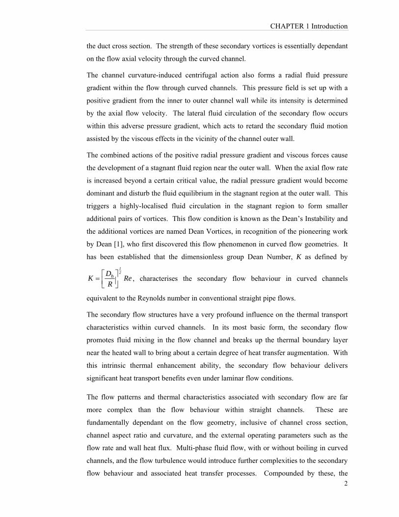
the duct cross section. The strength of these secondary vortices is essentially dependant
on the flow axial velocity through the curved channel.
The channel curvature-induced centrifugal action also forms a radial fluid pressure
gradient within the flow through curved channels. This pressure field is set up with a
positive gradient from the inner to outer channel wall while its intensity is determined
by the axial flow velocity. The lateral fluid circulation of the secondary flow occurs
within this adverse pressure gradient, which acts to retard the secondary fluid motion
assisted by the viscous effects in the vicinity of the channel outer wall.
The combined actions of the positive radial pressure gradient and viscous forces cause
the development of a stagnant fluid region near the outer wall. When the axial flow rate
is increased beyond a certain critical value, the radial pressure gradient would become
dominant and disturb the fluid equilibrium in the stagnant region at the outer wall. This
triggers a highly-localised fluid circulation in the stagnant region to form smaller
additional pairs of vortices. This flow condition is known as the Dean’s Instability and
the additional vortices are named Dean Vortices, in recognition of the pioneering work
by Dean [1], who first discovered this flow phenomenon in curved flow geometries. It
has been established that the dimensionless group Dean Number, K as defined by
ReR
DK
21
h
, characterises the secondary flow behaviour in curved channels
equivalent to the Reynolds number in conventional straight pipe flows.
The secondary flow structures have a very profound influence on the thermal transport
characteristics within curved channels. In its most basic form, the secondary flow
promotes fluid mixing in the flow channel and breaks up the thermal boundary layer
near the heated wall to bring about a certain degree of heat transfer augmentation. With
this intrinsic thermal enhancement ability, the secondary flow behaviour delivers
significant heat transport benefits even under laminar flow conditions.
The flow patterns and thermal characteristics associated with secondary flow are far
more complex than the flow behaviour within straight channels. These are
fundamentally dependant on the flow geometry, inclusive of channel cross section,
channel aspect ratio and curvature, and the external operating parameters such as the
flow rate and wall heat flux. Multi-phase fluid flow, with or without boiling in curved
channels, and the flow turbulence would introduce further complexities to the secondary
flow behaviour and associated heat transfer processes. Compounded by these, the
CHAPTER 1 Introduction
3
secondary flow behaviour is not fully comprehended by the current state of published
research in this area.
In reported literature, the early attempts on curved duct research were confined to
experimental studies, which primarily focussed on visualisation methods to understand
the secondary flow characteristics. These were limited in scope due to measurement
constraints and flow control difficulties. Rectangular duct geometries have been
traditionally considered in these investigations on curved ducts. By virtue of shape,
such ducts offer less flow confinement for secondary vortex formation, making it
relatively easier for experimentation, including flow visualisation and numerical
modelling. Ducts with elliptical and circular cross sections have been lightly treated in
research in spite of being common and popular channel geometries used in industrial
and technological systems.
With the advent of advanced computational tools and methodologies, extended
opportunities are now available for precise numerical simulations and parametric
investigations, by which the curved channel flow behaviour can be analysed for deeper
and improved understanding. In these, a major challenge is to synthesise more realistic
numerical formulations that are congruent with the complex nature of the secondary
flow vortex motion. In this regard, almost all reported numerical simulations up to now
have significant modelling deficiencies, in terms of geometrical range of applicability,
consistency of results and parametric considerations. The parametric influences of the
channel geometry and the flow variables remain unexplored and poorly understood.
Additionally, there are no decisive techniques for defining or identifying the onset of
Dean’s Instability and, the formation of Dean vortices and their locations. Most of
these models do not accommodate the temperature dependency of fluid properties
variations leading to unrealistic predictions, especially with heated curved channels.
Majority of reported models are limited to single-phase fluid flow systems and, are not
adaptable or conducive for multi-phase fluid flows. In this latter type of fluid flow,
specific requirements exist to capture the distribution of fluid phases and account for the
physical interaction across phases through heat and mass transfer processes, interfacial
evaporation and surface tension effects.
CHAPTER 1 Introduction
4
1.2. Scope of work
The study presented in this thesis is carefully developed and carried out to address
many of the above-mentioned shortcomings in the current state of fundamental
knowledge and analytical methodologies in secondary flow behaviour within heated
curved channels. Formulating necessary User Defined Functions (UDF) for the
computational fluid dynamics software FLUENT, the study develops novel
simulations models for single and multi-phase fluid flows through curved channels
having several practical cross sectional geometries. These models incorporate flow
parameters and mesh arrangements that are highly congruent with the secondary
vortex structures compared to previous models for much realistic representation of
intricate flow features. As a critical analytical tool for this field of research, the study
also develops two intuitive approaches for detecting the onset of Dean Instability with
an appraisal of their merits. An optimisation scheme is developed and tested for
curved passages in achieving most effective thermal performance for a given set of
parametric conditions and geometry.
In discussing above details, the thesis is broadly arranged to provide the aspects that
are specific to the individual situations of single phase, immiscible two-phase and two-
phase boiling fluid flows through curved channels.
1.3. Research Objectives
This research study examines the fluid flow and heat transfer characteristics in curved
channels for single and two-phase fluid flows. In the latter case, both immiscible (or
non-mixing) two-phase mixtures and the fluid flow boiling are considered. Fluid and
thermal characteristics are appraised with regard to secondary flow features and
parametric influences within rectangular, elliptical and circular channel geometries.
In view of these, the objectives of the study are as follows:
(a) For single-phase fluid flow in curved channels:
Improving on current modelling limitations, a novel three-dimensional
simulation approach is developed for single phase fluid flow through curved
rectangular, elliptical and circular geometries. Suitable mesh arrangements are
considered with the necessary capabilities in capturing intricate details of

CHAPTER 1 Introduction
5
secondary vortex formation and to achieve high consistency of results. The
model is validated against the published experimental data.
In fulfilling a critical need for this field of research, practical and accurate
criteria are formulated to identify the onset of Dean’s Instability and Dean
vortex generation. These are appraised for their suitability for various channel
geometries under consideration.
Above single-phase model is deployed to investigate the fluid behaviour within
rectangular, elliptical and circular channels in terms of fluid flow rate, channel
aspect ratio and wall heat flux.
A thermal optimisation scheme is developed for the fluid flow through curved
channels.
(b) For immiscible two-phase fluid flow in curved channels:
Accounting for the simultaneous flow of two non-mixing fluid components
within a curved passage, a new three-dimensional simulation is developed
specifically for this type of two-phase flow in a circular channel. Suitable
mesh arrangements are considered with the necessary capabilities in capturing
the distribution of immiscible fluid phases, unique features arising from
momentum transfer between phases and the details of secondary vortex
formation in each fluid phase. The model consistency is tested and established.
Above immiscible two-phase model is deployed to investigate the fluid
behaviour in a circular channel within each fluid phase, identifying the
interactive nature of centrifugal forces and momentum transfer across phase
boundaries. Thermal characteristics unique to this type of flow are examined
with appropriate physical explanations.
A thermal optimisation scheme is developed for this two-phase fluid flow
through curved channels.
(c) For two-phase flow boiling in curved channels:
Above single-phase model is modified and extended to two-phase flow boiling
situation by considering wall heat partitioning techniques, where both mass
and heat transfer are considered with the phase interfacial momentum transfer.
This new approach represents the most accurate to-date in terms of physical

CHAPTER 1 Introduction
6
mechanisms involved among two-phase flow models for this type of fluid flow
with boiling.
The model is deployed to examine the unique characteristics of phase
distribution and boiling heat transfer in circular channels whereby special flow
features are identified.

CHAPTER 2 Literature Survey
7
CHAPTER 2
CHAPTER 2 Literature Survey
2.1. Secondary flow and hydrodynamic instability
The pioneering experimental work on the secondary flow and hydrodynamic instability
was carried out by Eustice [1], investigating the resistance against fluid flow in metal
pipes - both straight and curved. First, the concept of critical velocity (threshold of
transient regime) was shown to be extended to a higher flow rate for curved pipes and,
then he reported new proportion of fluid with velocity below critical fluid velocity.
These experiments showed that the flow rate in a curved channel to be proportional to
the velocity raised to the power “n”. Further work by Eustice [2] showed the flow
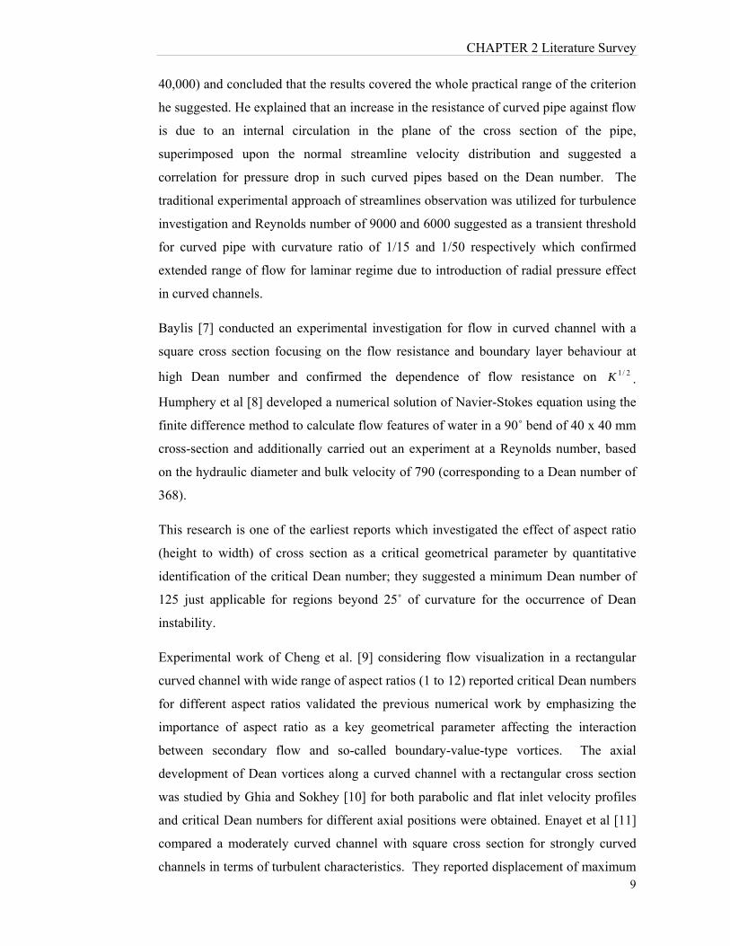
pattern in a curved channel by visualizing streamlines. Figure 2.1 shows the test set-up
used by Eustice [2] wherein he observed streamlines based on the location of dye
injectors This was the first published work on the description of secondary flow in
curved pipes which also qualitatively discussed the parametrical effect of flow and
geometry effect, and the critical flow rate extension.
Figure 2.1. Eustice’s experimental arrangement [2]
The first analytical and numerical work was established by Dean [3] in a coiled pipe
with a circular cross section in an attempt to model what Eustice had reported
experimentally demonstrating the complicated and unique behaviour of streamlines in
such a field. Assuming small curvature ratio (diameter of pipe to radius of curvature)
CHAPTER 2 Literature Survey
8
and consequently negligible axial velocity gradient Dean managed to obtain a good
qualitative agreement between his model and experimental model.
The results from this work showed the effect of flow rate on pressure drop and
confirmed that pressure drop does not change linearly with Reynolds number and
accordingly introduced effective dimensionless ratio in curved channels. Using stream-
function definition he analytically proved flow features and streamline arrangements are
related to the ratio of 2ReR
D , where D and R are the diameter of tube and curvature
radius, respectively. The model was utilized to investigate flow streamlines in a given
cross section of pipe to demonstrate secondary flow and counter rotating vortices in top
and bottom sides of the cross section; moreover, by tracking streamlines in a plane at
the middle of pipe, the study provided the longitudinal distance along coiled pipe at
which a certain streamline moves from outer wall to inner wall. Two points were
concluded out of these demonstrations; first the spiral motion of streamlines and then
effect of flow rate (in laminar regime) on vortex structure. As an extension of this
work, Dean published two reports [4,5] that provided an analytical correlation for
pressure drop versus bulk flow velocity in curved channels. Dean modified initial
definition of influential dimensionless number in curved channels to what is known as
the Dean number ( Re)( 2/1
R
DK ) and explained its effect for different curvature ratios.
Another important aspect of this research was identifying a new type of instability for
curved channels which was fundamentally different from turbulence. Beyond a certain
flow rate, far below the turbulence threshold, streamlines were found to be broken in
some flow areas where the flow was steady and incompressible. Dean’s numerical
model showed that a type of small disturbance which could not persist in a straight
channel is possible in a curved channel. Parabolic velocity profile previously proved
for pipe flows was showed to be inconsistent for curved channels.
Dean's work was of utmost value in that he pointed to a basis of correlation describing a
particular feature of fluid flow in a curved channel.
White [6] carried out experimental work over a range of flows at least twice as great as
that investigated by Eustice to explore the relation between Dean number and pressure
drop in curved and coiled pipes. Using oil with different densities and water, White
succeeded to carry out the experiment over a wide range of Reynolds numbers (0.06 to
CHAPTER 2 Literature Survey
9
40,000) and concluded that the results covered the whole practical range of the criterion
he suggested. He explained that an increase in the resistance of curved pipe against flow
is due to an internal circulation in the plane of the cross section of the pipe,
superimposed upon the normal streamline velocity distribution and suggested a
correlation for pressure drop in such curved pipes based on the Dean number. The
traditional experimental approach of streamlines observation was utilized for turbulence
investigation and Reynolds number of 9000 and 6000 suggested as a transient threshold
for curved pipe with curvature ratio of 1/15 and 1/50 respectively which confirmed
extended range of flow for laminar regime due to introduction of radial pressure effect
in curved channels.
Baylis [7] conducted an experimental investigation for flow in curved channel with a
square cross section focusing on the flow resistance and boundary layer behaviour at
high Dean number and confirmed the dependence of flow resistance on 2/1K .
Humphery et al [8] developed a numerical solution of Navier-Stokes equation using the
finite difference method to calculate flow features of water in a 90˚ bend of 40 x 40 mm
cross-section and additionally carried out an experiment at a Reynolds number, based
on the hydraulic diameter and bulk velocity of 790 (corresponding to a Dean number of
368).
This research is one of the earliest reports which investigated the effect of aspect ratio
(height to width) of cross section as a critical geometrical parameter by quantitative
identification of the critical Dean number; they suggested a minimum Dean number of
125 just applicable for regions beyond 25˚ of curvature for the occurrence of Dean
instability.
Experimental work of Cheng et al. [9] considering flow visualization in a rectangular
curved channel with wide range of aspect ratios (1 to 12) reported critical Dean numbers
for different aspect ratios validated the previous numerical work by emphasizing the
importance of aspect ratio as a key geometrical parameter affecting the interaction
between secondary flow and so-called boundary-value-type vortices. The axial
development of Dean vortices along a curved channel with a rectangular cross section
was studied by Ghia and Sokhey [10] for both parabolic and flat inlet velocity profiles
and critical Dean numbers for different axial positions were obtained. Enayet et al [11]
compared a moderately curved channel with square cross section for strongly curved
channels in terms of turbulent characteristics. They reported displacement of maximum

velocity to
on the inn
layers rem
were repor
Sugiyama
flow and
Figure 2.2
K=F
Based on
developme
pattern of
addition t
developed
region dev
aspect rati
ratio from
number fo
they left
investigate
some diffe
flow instab
Chandratil
curvature
was effect
function a
o the outsid
ner wall. Ac
mained thin.
rted to be h
a et al [12] c
reported th
2 the flow pa
127
Figure 2.2. C
the obtained
ent into thr
f cross secti
to main sec
d by retarded
velops new
io less than
m 1 to 2; ho
or each aspe
this area
ed the flow
ferences com
bility.
lleke et al [
ratio, aspec
tively a 2-d
approach wi
e of the ben
ccordingly in
. Turbulen
higher at inn
conducted a
he effect of
attern chang
K=Cross sectio
(exper
d flow visu
ree steps. Fi
onal flow,
condary vo
d layer. Th
w pairs of v
n 1 as comp
owever, thei
ect ratio to
without an
w field and
mpared to r
[14] report
ct ratio and
dimensional
ith dynamic
nd and resul
nward flow
nce intensity
ner corners o
an experime
aspect ratio
ges as a resu
=180 onal view ofriment by Su
ualization th
irst, the occ
then, occur
ortices and
he report def
vortices and
pared to 2,
ir experime
clearly cap
ny discussi
vortices for
rectangular
an extensiv
d external w
l model inco
c similarity
lted in an ac
ws at the side
y and shear
of cross sec
ent to descri
o and curva
ult of flow r
K=f flow patterugiyama et
hey classifie
currence of
rrence of re
finally the
fined critica
d suggested
and then an
ental techniq
pture the cro
ion. Dong
rmed in ell
channels in
ve parametr
wall heat flu
orporating t
y in axial di
CHAPTE
ccumulation
e-walls ensu
r stress mea
tion at the o
ibe the deve
ature ratio.
rate increas
=224 rn at the endal [12])
ed the seque
f secondary
tarded laye
inception
al Dean num
higher crit
n abrupt ris
que failed b
oss-sectiona
and Ebad
liptical curv
n the forma
ric study ex
ux. Their n
toroidal coo
irection. In
ER 2 Literat
n of slow m
ured that th
asured in th
outlet plane
elopment of
As it is ev
e in curved
K=d of curvatu
ence of seco
flow as a w
r near to ou
of addition
mber at whi
tical Dean n
se for chang
beyond a ce
al vortex str
dian [13] n
ved channel
ation of the
xamining the
numerical f
ordinates an
ntersecting c
ture Survey
10
moving fluid
he boundary
his research
.
f secondary
vident from
channels.
=391 ure
ondary flow
well-known
uter wall in
nal vortices
ich retarded
number for
ging aspect
ertain Dean
ructure and
numerically
ls, reported
e secondary
e effects of
formulation
nd a stream
contours of
y
0
d
y
h
y
m
w
n
n
s
d
r
t
n
d
y
d
y
f
n
m
f

CHAPTER 2 Literature Survey
11
stream function were adapted as a qualitative criterion for establishing the occurrence of
flow instability and Dean vortices. Chandratilleke et al [14, 29, 30] presented results for
rectangular ducts for a comprehensive range of Dean numbers 25 ≤ K ≤ 500, aspect
ratio 1 ≤ Ar ≤ 8. They represented a trend for the variation of the critical Dean number
versus the aspect ratio and curvature ratio, which confirmed the trends observed in
Cheng et al [9] with some modification based on their qualitative stream function
approach.
In an attempt to define a quantitative criterion to identify the onset of Dean instability,
Fellouah et al [15] conducted a numerical-experimental analysis. They used the finite-
volume CFD package to solve the three-dimensional Navier-Stokes equation for
laminar, incompressible flow. They also had a well-controlled water tunnel with long
entrance section and a curved testing section for flow visualization using the LIF (Laser
induced florescence) technique. They suggested that the radial gradient of the axial
velocity measured along the line connecting eye to eye of the Dean vortices as a
criterion for Dean instability inception and compared their prediction, based on defined
criterion, with LIF flow visualization.
K=80 K=150 Radial gradient of axial
velocity
Figure 2.3. Quantitative assessment of instability inception by Fellouah et al [15]
The criterion delivered an original attempt of quantitative assessment of instability; yet,
was not generalized regarding of geometry and flow rate since it was not possible to
predict the exact position of Dean vortices’ eye for different geometries and flow
conditions as shown in Figure 2.3. The critical Dean numbers for different aspect and
curvature ratios did not suggest considerable difference with the previous two-
dimensional numerical models or classic experimental studies by Cheng et al [9] or
Ghia and Sokhey [10]. Their study investigated the concept of fully development
CHAPTER 2 Literature Survey
12
length in curved channels for mentioned inlet velocity profiles and suggested different
correlations for cross section of rectangular cross section. Helin et al [16] used a finite
volume numerical model to investigate secondary flow and Dean instability with a
shear-thinning Phan-Thien–Tanner fluid in a U-curved channel of square section for
tiny range of Dean number (125≤K≤150). The first results of this research obtained a
lower flow rate required for the transition to the four-cell structure (known as Dean
instability threshold) for viscoelastic fluid as compared to Newtonian fluid with the
same condition as the inertial term is increased. Moreover, for explored range of Dean
numbers they established that increasing the power-law index n of the Phan- Thien–
Tanner model retards the onset of additional Dean vortices; in contrast, additional
computations with an Oldroyd-B fluid demonstrated that the size and intensity of the
secondary vortices present in the four-cell pattern increase with elasticity.
Fellouah et al [17] later used their own developed quantitative criterion to identify the
effect of rheological fluid behaviour on the Dean instability of power-law and Bingham
fluids in curved rectangular ducts. Their results confirmed a decrease in the critical
Dean number as a result of power law index increase and showed an opposite effect for
Bingham number. Variation of rheological parameters however was found to be merely
effective on position of vortices and not on size of them and the flow visualization
showed that the effect of the yield stress on the shape of the flow to be the dominant
parameter.
2.2. Thermal behaviour with secondary flow
Secondary flow which is basically due to centrifugal effect is a lateral-cross sectional
motion of fluid results in an increase in the mixing rate. Accordingly the rate of
convective heat transfer is substantially increased by the new main and extra vortices in
the flow field. Moreover, the contribution of the extra body force due to buoyancy effect
for a given flow rate and material properties will be considerable resulting in a mutual
interaction between buoyancy and centrifugal source terms. Common application of
curved channel and tubes in addition to the importance of the unique physics of heat
transfer in such flow fields has attracted researchers during past decades. Accordingly,
extensive numerical and experimental reports are available in literature regarding the
mutual effect of heating and curvature on flow field and heat transfer in curved confined
geometries.
CHAPTER 2 Literature Survey
13
Cheng et al [18] conducted a numerical analysis of forced convection in a curved
channel with rectangular cross section, investigating the velocity and temperature fields
as well as Nusselt number on the heated wall. The study included a dimensionless
parameter analysis investigating the effect of critical values such as flow rate, aspect
ratio and Prandtl number on the velocity and temperature profiles in comparison with
correspondent values in a straight channel. The results suggested the trend for
temperature similar to velocity profile where the maximum value is pushed toward the
outer wall as Dean number increases. The effect of aspect ratio on the flow field was
found to displace the centre of secondary vortices and consequently make a variation in
velocity and temperature field; however, Prandtl number was found to be just effective
on heat transfer and not on streamlines. Mori et al [19] reported a more detailed analysis
for hydro-thermal assessment of curved channel with a square cross section and by
assuming material properties to be temperature-independent, neglecting the effect of
temperature field on velocity and streamlines. They also conducted an experiment
using air as fluid and four independent heaters with constant heat flux on walls and
successfully validated their analytical solution up to Re=8000 including transition range
of flow for both velocity and Nusselt number. As a main contribution of this study,
they explained the structure of boundary layer region and the important effect of that on
both velocity and temperature fields by taking secondary flow effect into account for
obtaining boundary layer equation particularly for curved channels. The suggested
Nusselt number correlation, based on such an analysis, was showed to be more accurate
rather than previously reported estimations as compare to experimental results.
Tyagi and Sharma [20] published another study of laminar forced convection with
circular cross section taking viscous dissipation effect into account. They claimed the
presence of a marked distinction between thermal boundary condition cases of straight
and curved tubes when the cross-sections of both are circular due to circumferentially
non-uniform viscous dissipation. Based on such an assumption they carried out a
perturbation analysis to investigate the velocity and temperature field and consequently
assessed convective heat transfer by discussing Nusselt number. Their result,
interestingly, showed a reversed effect of viscous dissipation rate in curved channel. An
analytical correlation for Nusselt number in curved channels, as a result, was modified
taking viscous heating effect into account.

CHAPTER 2 Literature Survey
14
Mixed convection flows in concentric curved annular ducts with constant wall
temperature boundary condition were studied numerically by Hoon [21]. He focused on
effect of radius ratio (ratio of the inner core radius to the outer pipe radius), the Dean
number and Grashof number on Nusselt number and friction factor. As one of the
earliest studies which highlighted the relative importance of centrifugal and buoyancy
forces in curved tubes, Hoon explained the secondary flow pattern exhibits a strong
asymmetry as a result Grashof number increase (i.e. increase of buoyancy force) when
the Dean number is low enough. On other hand, by increasing the Dean number, the
flow field was found to be pushed back to its almost symmetric pattern. Comparing two
different orders of Grashof number, results suggested a slight dependence of Nusselt
number and friction factor to either Dean number or radius ratio for 12500Gr
whereas these ratios increase as either the radius ratio increases or Dean number,
contrary to the case of 5.12Gr .
Targett et al [22] solved the equations for the conservation for mass, momentum and
energy for fully developed angular flow and fully developed convection in the annulus
between two concentric cylinders. Flow was assumed to have invariant physical
properties, Newtonian behaviour and negligible viscous dissipation and accordingly
reported Nusselt number to be mostly dependent on heat flux density ratio as well as
Dean number. They assessed Nusselt number for complete range of heat flux density
ratios, (both positive and negative), on the inner and outer surfaces, for Dean numbers
up to 2.5 times the critical value for the onset of vertical motion and the computed
results were concluded to be applicable, within some mentioned geometrical
restrictions, as a good approximation for true double-spiral heat exchangers in terms of
the local Dean number. The effect of Dean vortices on forced convection was studied
by Ligrani and Choi [23]; to accomplish this task, buoyancy influences were minimized
by orienting the channel so that gravity acted in the span-wise direction perpendicular to
the bulk flow direction and additionally, a new procedure was applied to deduce forced
convection Nusselt numbers from Nusselt numbers measured in a mixed convection
environment with relatively weak buoyancy. In given procedure, Nusselt numbers at
different T were measured, by varying heating power, and then measured data are
extrapolated to 0T which gives forced convection Nusselt numbers with no
buoyancy influences. Comparing concave and convex walls they reported the Nusselt
number exceeding significantly at concave (outer) wall over a certain Dean number (or
longitudinal length of channel) due to secondary flows which result as tiny Gortler-like
CHAPTER 2 Literature Survey
15
vortices start to form near the concave surface of the channel. They later
experimentally compared mixed convection in straight and curved channels with
buoyancy orthogonal to the forced flow [24].
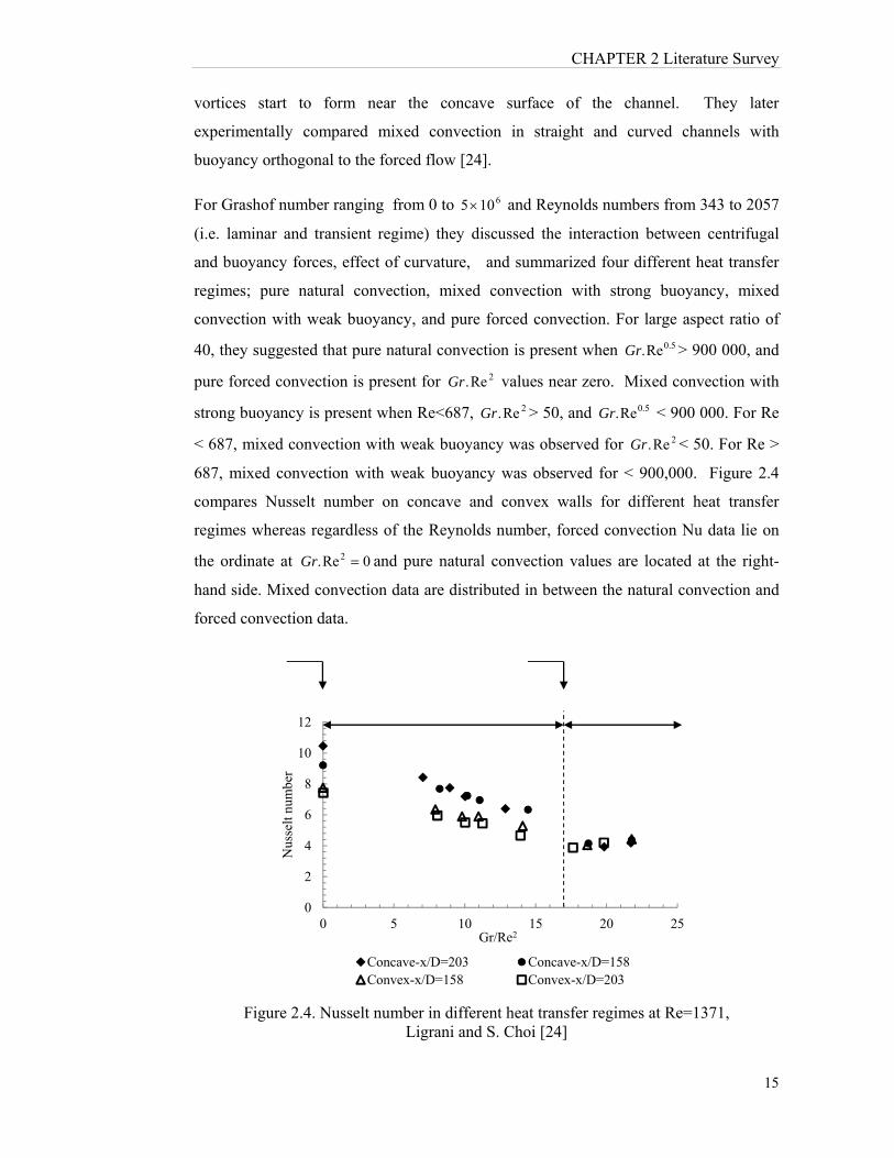
For Grashof number ranging from 0 to 6105 and Reynolds numbers from 343 to 2057
(i.e. laminar and transient regime) they discussed the interaction between centrifugal
and buoyancy forces, effect of curvature, and summarized four different heat transfer
regimes; pure natural convection, mixed convection with strong buoyancy, mixed
convection with weak buoyancy, and pure forced convection. For large aspect ratio of
40, they suggested that pure natural convection is present when 5.0Re.Gr > 900 000, and
pure forced convection is present for 2Re.Gr values near zero. Mixed convection with
strong buoyancy is present when Re<687, 2Re.Gr > 50, and 5.0Re.Gr < 900 000. For Re
< 687, mixed convection with weak buoyancy was observed for 2Re.Gr < 50. For Re >
687, mixed convection with weak buoyancy was observed for < 900,000. Figure 2.4
compares Nusselt number on concave and convex walls for different heat transfer
regimes whereas regardless of the Reynolds number, forced convection Nu data lie on
the ordinate at 0Re. 2 Gr and pure natural convection values are located at the right-
hand side. Mixed convection data are distributed in between the natural convection and
forced convection data.
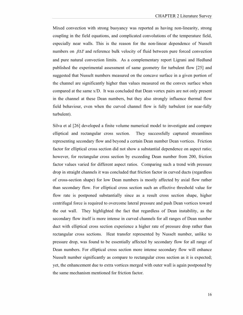
Figure 2.4. Nusselt number in different heat transfer regimes at Re=1371, Ligrani and S. Choi [24]
0
2
4
6
8
10
12
0 5 10 15 20 25
Nus
selt
num
ber
Gr/Re2
Concave-x/D=203 Concave-x/D=158Convex-x/D=158 Convex-x/D=203
CHAPTER 2 Literature Survey
16
Mixed convection with strong buoyancy was reported as having non-linearity, strong
coupling in the field equations, and complicated convolutions of the temperature field,
especially near walls. This is the reason for the non-linear dependence of Nusselt
numbers on T and reference bulk velocity of fluid between pure forced convection
and pure natural convection limits. As a complementary report Ligrani and Hedlund
published the experimental assessment of same geometry for turbulent flow [25] and
suggested that Nusselt numbers measured on the concave surface in a given portion of
the channel are significantly higher than values measured on the convex surface when
compared at the same x/D. It was concluded that Dean vortex pairs are not only present
in the channel at these Dean numbers, but they also strongly influence thermal flow
field behaviour, even when the curved channel flow is fully turbulent (or near-fully
turbulent).
Silva et al [26] developed a finite volume numerical model to investigate and compare
elliptical and rectangular cross section. They successfully captured streamlines
representing secondary flow and beyond a certain Dean number Dean vortices. Friction
factor for elliptical cross section did not show a substantial dependence on aspect ratio;
however, for rectangular cross section by exceeding Dean number from 200, friction
factor values varied for different aspect ratios. Comparing such a trend with pressure
drop in straight channels it was concluded that friction factor in curved ducts (regardless
of cross-section shape) for low Dean numbers is mostly affected by axial flow rather
than secondary flow. For elliptical cross section such an effective threshold value for
flow rate is postponed substantially since as a result cross section shape, higher
centrifugal force is required to overcome lateral pressure and push Dean vortices toward
the out wall. They highlighted the fact that regardless of Dean instability, as the
secondary flow itself is more intense in curved channels for all ranges of Dean number
duct with elliptical cross section experience a higher rate of pressure drop rather than
rectangular cross sections. Heat transfer represented by Nusselt number, unlike to
pressure drop, was found to be essentially affected by secondary flow for all range of
Dean numbers. For elliptical cross section more intense secondary flow will enhance
Nusselt number significantly as compare to rectangular cross section as it is expected;
yet, the enhancement due to extra vortices merged with outer wall is again postponed by
the same mechanism mentioned for friction factor.
CHAPTER 2 Literature Survey
17
Andrade et al [27] investigated the effect of temperature dependent viscosity on heat
transfer and velocity profile for a fully developed forced convection case in a curved
duct using a finite element model. They analysed both cooling and heating cases and
under cooling conditions, the Nusselt values with variable-viscosity were found to be
lower than the constant-properties results due to the increase of the viscosity at the inner
points of the curved tube section that reduces the secondary flow effects and the heat
transfer rate.
An experimental study performed by Christopher and Mudawar [28], discussed the
enhancement mechanism of heat transfer in curved channel for a fully turbulent regime.
They first compared stream-wise Nusselt number variation for straight and curved
channels and obtained different thermally fully developed region for each case. At a
location close to the inlet, the Nusselt number was found to be almost the same as those
obtained for straight channel. It showed that it takes a finite distance for the secondary
flows to develop and influence the heat transfer as previously for laminar flow
secondary flow was suggested to be effective beyond turn angles 15 . Further
downstream of this point they obtained an enhancement ratio defined as
1.0046.0 )2
(ReR
D
Nu
Nu h
straight
curved and improved the former available correlations by 6%.
Chandratilleke et al [29] has used the idea of secondary flow to optimize heat exchanger
performance based on former studies. Following this study, they conducted an
experiment [30] to investigate mutual effect of heating and centrifugal force in curved
channel with rectangular cross section; in which they experimentally assessed a wide
range of effective parameters by view of flow visualization and heat transfer analysis.
They used air as the main flow and smoke as flow indicator and managed to capture
cross sectional view of vortices structure in different cross section through curved duct.
Their result showed the most vivid prospect of centrifugal versus buoyancy force
interaction qualitatively where the effect of geometrical parameters (e.g. aspect ratio,
curvature ratio and hydraulic diameter) was demonstrated. Beyond a mere qualitative
assessment, their important work [13] which was the most comprehensive numerical
model up to the time, used a finite volume CFD code for incompressible laminar flow
which was validated against their own former experiment and utilized stream-function
for instability analysis of vortex structure whereas curved section was uniformly
heated. Using Boussinesq approximation, the effect of buoyancy force was taken into
CHAPTER 2 Literature Survey
18
account and the precise assessment of interaction between that with centrifugal force
was carried out. As it is evident from Figure 2.5, for a non-heated channel the
centrifugal force merely is affecting flow field leads a symmetrical vortex structure
where the Dean vortices are apparent next to the outer wall; nevertheless, by applying
heating buoyancy will perform as a vertical driven flow and significantly changes flow
domain. The unbalanced secondary vortex motion found to enhance fluid velocities
parallel to the outer wall in the top half of the duct and impede fluid velocities in the
bottom half. Combined with the repositioning of the stagnant region, this velocity
imbalance near the outer wall reduces the formation potential of flow reversal cells for a
given aspect ratio. Hence, the Dean vortices are diminished in number with the
application of external heating on the outer wall of curved ducts.
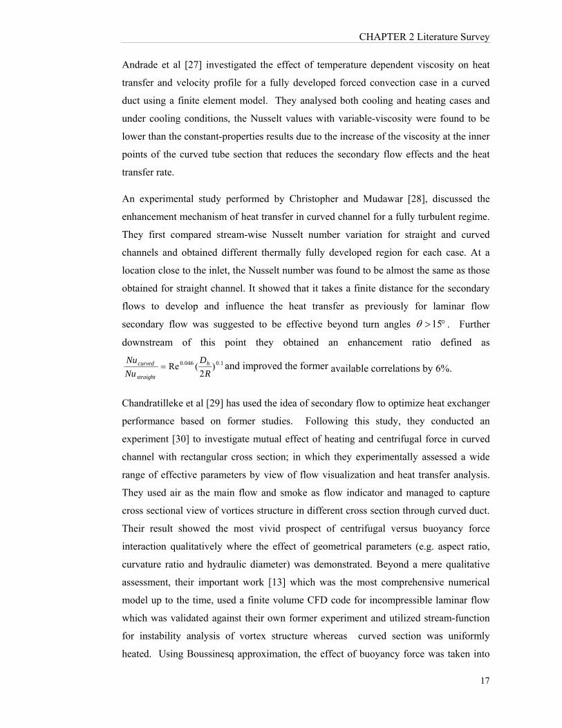
a) non-heated wall b) partially heated channel
(q=25W/m2)
Figure 2.5. Effectiveness of buoyancy; assessment of stream function versus flow visualization at the curvature exit (θ=180, K=380, Ar=4) [13]
They reported an intense temperature gradient at the outer wall of the duct and an
unsymmetrical temperature field in the fluid at lower flow rates due to thermal
stratification. As the flow rate increases, the temperature field gradually acquires the
symmetry associated with the stronger secondary flow-vortex motion. It was seen that
for a given duct aspect ratio, increasing flow rate leads to gradual enhancement of
Nusselt number. This research observed that the Nusselt number for a curved duct is
20–70% higher than that of a corresponding straight passage. This heat transfer
enhancement was justified with two operating mechanisms; the secondary vortex
motion gives a rise to higher fluid velocities at the outer wall and causes rapid removal
of the hotter fluid there and shifting of flow distribution towards the outer wall causes
thinning of the thermal boundary layer at the heated wall, (as indicated by their

CHAPTER 2 Literature Survey
19
temperature distribution) and leads to reduced thermal resistance to heat flow from the
heated boundary to the fluid. They finally assessed the effect of aspect ratio on
convective heat transfer and obtained higher Nusselt number for larger aspect ratio since
more number of Dean vortices will be produced by increasing aspect ratio.
Yanase et al [31] analyzed a non-isothermal curved duct with a rectangular cross section
fixed at aspect ratio of 2 using the spectral method. Their numerical research explored
the linear instability and heat transfer for the case of heated outer and cooled inner wall,
where parametric analysis was carried out over the range of 1000100 Gr
and
10000 K . They assessed the range of Dean numbers for two Grashof number of
500 and 1000 in detail and obtained five branches of steady solution using the Newton-
Raphson iteration method for either of cases. Accordingly, they studied linear stability
of each branch with respect to two-dimensional perturbations and suggested unexpected
results. It was found that among multiple steady solutions obtained, only one steady
solution is linearly stable for a single range of the Dean number for 500Gr , for
1000Gr , on the other hand, linear stability region exists in three different intervals of
the Dean number on the same branch. Unsteady analysis of the flow show that for
500Gr , the laminar flow turns into chaotic through a time periodic state in a
straightforward way (i.e. steady–periodic–chaotic), for 1000Gr , on the other hand, the
flow undergoes (i.e. steady–periodic–steady– periodic–steady–periodic–chaotic), as the
Dean number increases. As a heat transfer assessment of field, they compared Nusselt
number for all cases of steady, periodic and chaotic flow and reported a general increase
due to curvature effect and a specific rise due to periodic and chaotic effect for those
given ranges of Dean number.
Ko et al extensively assessed entropy generation analysis in curved channel field [32-
35]. They first developed a finite volume CFD model which recognized the influential
parameters on irreversibility due to either heat transfer or fluid friction terms [32]. For a
partially heated channel with rectangular cross section they showed that for a given heat
flux by increasing flow rate, FFI (fluid friction irreversibility) gradually increase and at
the certain flow rate overcomes HTI (heat transfer irreversibility) which means
volumetric average Bejan number approaches form 0 to 1. Ko et al studied the effect of
longitudinal ribs on heat transfer and pressure drop in curved channels [33, 34]
numerically. Calculation of cases with various rib size under different Dean number and
heat flux revealed that addition of ribs can effectively reduce entropy generation from
CHAPTER 2 Literature Survey
20
heat transfer irreversibility since augmentation of secondary vortices makes temperature
gradient smoother. In turn, entropy generated by fluid friction irreversibility rise up due
to wider solid walls and the complex flow disturbed by ribs. Analysis of the optimal
trade-off was carried out based on the minimal total entropy generation principle and
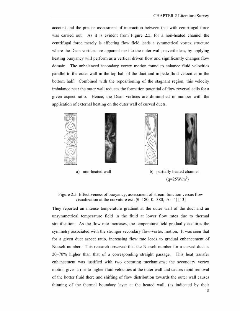
optimal rib size suggested to be dependent on Dean number and heat flux. Figure 2.6
illustrates variation of Bejan number (ratio of HTI to total entropy generation)
throughout a 180 curved section.
Outer heated wall located at right, K=1000, 112.0.
.
in
h
Tk
DQ
Figure 2.6. Local Bejan number for different number of ribs in different angular position through curved section [34]
Their extensive contribution includes another study on the flow and heat transfer
characteristics in curved ducts for a turbulent regime [35]. In presence of turbulence
energy cascade, new terms which influence entropy generation, were considered and
well established methodology of trade-off analysis for entropy generation carried out.
A substantial increase in FFI was justified due to the introduction of turbulent Reynolds
stress terms where aspect ratio was found to have a remarkable direct effect on
enhancement of total entropy generation due to FFI.
Wang and Liu [36] addressed the effect of curvature on bifurcation structure and
stability of forced convection in slightly forced micro-channels with a numerical study.
They suggested that no matter how small the channel’s cross-section is; the channel
CHAPTER 2 Literature Survey
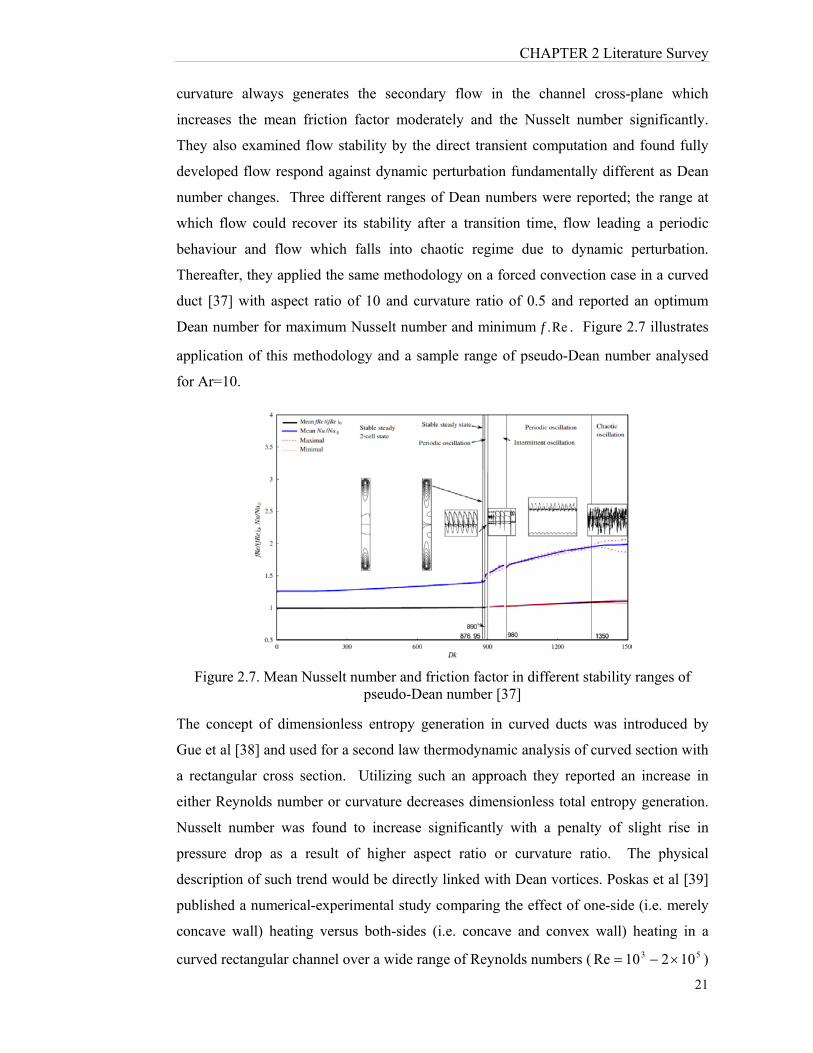
21
curvature always generates the secondary flow in the channel cross-plane which
increases the mean friction factor moderately and the Nusselt number significantly.
They also examined flow stability by the direct transient computation and found fully
developed flow respond against dynamic perturbation fundamentally different as Dean
number changes. Three different ranges of Dean numbers were reported; the range at
which flow could recover its stability after a transition time, flow leading a periodic
behaviour and flow which falls into chaotic regime due to dynamic perturbation.
Thereafter, they applied the same methodology on a forced convection case in a curved
duct [37] with aspect ratio of 10 and curvature ratio of 0.5 and reported an optimum
Dean number for maximum Nusselt number and minimum Re.f . Figure 2.7 illustrates
application of this methodology and a sample range of pseudo-Dean number analysed
for Ar=10.
Figure 2.7. Mean Nusselt number and friction factor in different stability ranges of pseudo-Dean number [37]
The concept of dimensionless entropy generation in curved ducts was introduced by
Gue et al [38] and used for a second law thermodynamic analysis of curved section with
a rectangular cross section. Utilizing such an approach they reported an increase in
either Reynolds number or curvature decreases dimensionless total entropy generation.
Nusselt number was found to increase significantly with a penalty of slight rise in
pressure drop as a result of higher aspect ratio or curvature ratio. The physical
description of such trend would be directly linked with Dean vortices. Poskas et al [39]
published a numerical-experimental study comparing the effect of one-side (i.e. merely
concave wall) heating versus both-sides (i.e. concave and convex wall) heating in a
curved rectangular channel over a wide range of Reynolds numbers ( 53 10210Re )
CHAPTER 2 Literature Survey
22
and geometrical parameters ( 905/ aDh and 202/ abAr ). Critical Reynolds
number were reported to be identical for both case of one-side and two-side heating
whereas Nusselt number increase was observed by 50% for laminar-vortex flow and by
20% for turbulent flow regime for two-side heating as compare to one side heating.
An experimental work was conducted by Fu et al [40] to investigate the effects of a
reciprocating motion on mixed convection of a curved vertical cooling channel with a
heated top surface, and numerical work was executed simultaneously to validate the
experimental results. The experimental apparatus consisted of three main parts of a
cooling channel, reciprocating movement and heating control to control and measure
Reynolds numbers, frequencies, amplitudes and temperature differences. Heat transfer
enhancement was found to have a direct relation with frequency since contributions of
flow flowing and reciprocating motion to the heat transfer rate are mutually affected.
2.3. Secondary flow and centrifugal force in multi-phase domains
Multi-phase domain in a curved section subjected to centrifugal force behaves in
specific way, regarding phase arrangement and vortex structure. Since such a domain
consists of elements with different material properties such as density, viscosity and
thermal properties, first phase arrangement will be unique owing to centrifugal force.
Accordingly, secondary flow for fluid domain will be influenced by phase re-
arrangement and momentum exchange between phases. Given the unique features of
flow, this area has several applications in the industry such as phase separation, mixing
and optimized heating effect.
Gao et al [41] published a work contributing some knowledge of phase separation
phenomena of liquid–solid two-phase turbulent flow in curved pipes. They first
numerically simulated liquid-solid phase domain, using Euler–Lagrangian scheme, and
examined the effect of particle size, liquid flow-rate and coil curvature with different
assumptions regarding centrifugal force, drag force, pressure gradient force, gravity
force, buoyancy force, virtual mass force and lift force. They additionally conducted an
experiment using a nonintrusive Malvern 2600 particle sizer based on laser diffraction
to analyse the effect of secondary flow on phase separation. Their results suggested that
the solid particles with higher density as compare to liquid phase are driven to outer
bend due to centrifugal effect; however, by taking turbulence dispersion effect into
CHAPTER 2 Literature Survey
23
account trajectories becomes somewhat irregular which shows a negative effect of this
term on separation due to strong randomicity. Centrifugal force was found to be prime
driving force whereas the drag force and the pressure gradient play an opposite role for
separation, lift force is notable near the wall and helpful to separation and virtual mass
force could be omitted.
Shen et al [42] employed a 3D non-isotropic algebraic stress/flux turbulence model to
simulate turbulent buoyant helicoidal flow and heat transfer in a rectangular curved
open channel and by which reported a unique flow pattern including two major and one
minor secondary flow eddies in a cross section. The numerical results revealed that two
comparable eddies rotating in opposite directions are formed in cross sections of the
turbulent buoyant helicoidal flow in a curved open channel. The boundary between the
two eddies is located right in the thermocline This report was one of the early and
limited researches generally discussing structure of secondary flow for immiscible flow
through confined ducts and showed that the turbulence intensity is smaller in the
vertical and radial directions than the tangential direction due to turbulence suppression
by buoyancy and centrifugal forces. In contrast with the separation effect of curved
channel for immiscible phases (including solid-fluid mixture), curved ducts are possible
to be used for mixing enhancement due to additional lateral motion.
Kumar et al [43] numerically investigated the complex mixing regime of two miscible
fluids in a coil of circular cross section and obtained new trends and phase distributions.
Three-Dimensional grid was adopted in Cartesian coordinate system for this multi-
phase model whereas the two liquids were considered to have the same properties. Two
flows stream with inlet scalar concentrations of zero and unity in the two halves of a
tube perpendicular to the plane of curvature and were allowed to mix by convection and
diffusion. In straight tube the mixing is governed by a single parameter ( Sc.Re ), where
in a helical tube the mixing reported to be more complex because of the secondary flow
generation due to centrifugal forces that depend on the Reynolds number ( Re), Schmidt
number ( Sc ) and the curvature ratio. This research described that mixing in curved
tubes at intermediate Reynolds number is far more efficient than a straight tube of
similar dimensions. The mixing in curved tubes is significantly greater at higher
Reynolds numbers, whereas in straight tubes, mixing efficiency decreases as the
Reynolds number increases. Since in a curved tube, the increase in Reynolds number
produces increased levels of secondary flow, mixing would be enhanced. In contrast,
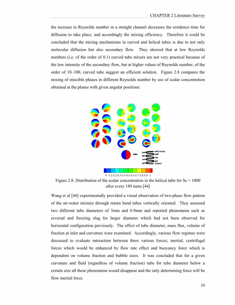
CHAPTER 2 Literature Survey
24
the increase in Reynolds number in a straight channel decreases the residence time for
diffusion to take place, and accordingly the mixing efficiency. Therefore it could be
concluded that the mixing mechanisms in curved and helical tubes is due to not only
molecular diffusion but also secondary flow. They showed that at low Reynolds
numbers (i.e. of the order of 0.1) curved tube mixers are not very practical because of
the low intensity of the secondary flow, but at higher values of Reynolds number, of the
order of 10–100, curved tube suggest an efficient solution. Figure 2.8 compares the
mixing of miscible phases in different Reynolds number by use of scalar concentration
obtained at the planes with given angular positions:
Figure 2.8. Distribution of the scalar concentration in the helical tube for Sc = 1000 after every 180 turns [44]
Wang et al [44] experimentally provided a visual observation of two-phase flow pattern
of the air-water mixture through return bend tubes vertically oriented. They assessed
two different tube diameters of 3mm and 6.9mm and reported phenomena such as
reversal and freezing slug for larger diameter which had not been observed for
horizontal configuration previously. The effect of tube diameter, mass flux, volume of
fraction at inlet and curvature were examined. Accordingly, various flow regimes were
discussed to evaluate interaction between three various forces; inertial, centrifugal
forces which would be enhanced by flow rate effect and buoyancy force which is
dependent on volume fraction and bubble sizes. It was concluded that for a given
curvature and fluid (regardless of volume fraction) tube for tube diameter below a
certain size all these phenomena would disappear and the only determining force will be
flow inertial force.

CHAPTER 2 Literature Survey
25
Fries and von Rohr [45] investigated the influence of the channel radius on the mass
transfer in rectangular meandering micro-channels (width 200–400 μm and height of
150μm) for gas–liquid flow. Laser induced velocimetry measurements were compared
with numerical results and the symmetrical velocity profile, known from the straight
channel, was found to change to an asymmetrical one for the meandering channel
configuration. As a result of this variation in velocity profile in the presence of
secondary flow, radial mass transfer enhanced inside liquid slug and resulted in a
reduced mixing length.
2.4. Flow boiling modelling
Tube boiling is another interesting phenomenon which is significantly influenced in
curved ducts due to centrifugal effect. Numerical investigation of tube boiling which is
inherently a multi-phase fluid domain having heat and mass transfer has been developed
by many researchers.
Luteset [46] used nitrogen and sapphire plate to investigate experimentally the transition
of nucleate to film boiling on a flat surface. The study reported instability in boiling
conditions and the transition between nucleate and film boiling regions, where the heat
flux observed was almost three times the critical heat flux for pool boiling. Using water
and refrigerant R113, Shiotsu and Hama [47] conducted forced convection film boiling
experiments in a vertical cylinder with the test liquid flowing upward. The effect of
parameters, such as flow rate, operating pressure, sub-cooled temperature were analysed
and a correlation was suggested for forced convection film boiling heat transfer with
thermal radiation. These results showed a good agreement with the published
experimental data. Based on liquid sub-layer dry out mechanism, Liu et al [48] have
developed one of the most up-to-date theoretical models for predicting critical heat flux
for sub-cooled flow boiling. This model has been conclusively validated against the
experimental data that spans almost the entire range of physical applicability. Their
parametric analysis involving mass flux, pressure, pipe diameter and heated length-to-
diameter ratio established the model consistency with non-uniform pipe heating and for
liquids such as water, nitrogen and R113.
Baduge et al [49] experimentally investigated the boiling heat transfer characteristic in
vertical capillary tubes under atmospheric pressure conditions. Within the parametric
CHAPTER 2 Literature Survey
26
range of mass flux (23.4 - 152.7 kg/m2s), heat flux (10 - 715 kW/m2) and dryness
fraction (0 - 0.8), they showed that in vertical capillary tubes, the slug-annular and
annular flow dominated the flow patterns while the liquid film evaporation was the
primary heat transfer mechanism. It was concluded that the boiling correlation for
normal sized tubes would under-predict heat transfer in capillary tubes.
Li et al [50] reported one of the early computational simulations on flow boiling, where
they modified the RPI approach and incorporated two-phase correlations into a CFX
model. This simulation was tested against the experimental results for flow boiling of
liquid nitrogen in a vertical tube, and showed a significant improvement in accuracy in
predicting the void fraction and wall temperature. Bostjan and Eckhard [51] have
successfully simulated convective boiling in vertical annulus obtaining good qualitative
agreement with experimental data. They illustrated that for two-phase modelling, the
Eulerian method was a very reliable approach for simulating turbulent sub-cooled
boiling although an over-prediction of velocity was evident in the near-wall regions.
This work examined the void fraction, phase velocity, turbulent kinetic energy and
temperature while investigating the effects of non-drag forces, bubble diameter and
interfacial drag models.
Two-phase flow boiling numerical models developed thus far are very sensitive in terms
of convergence and stability to the applied boundary conditions. In most cases, these
models fail to predict the critical heat flux (CHF) signalling of modelling shortfalls.
Sindhuja et al [52] have reported a much-improved numerical simulation, where they
studied a vertical tube carrying R-407C refrigerant and uniformly heated with wall heat
flux exceeding CHF. This work over- predicted the heat transfer rates compared to
three established correlations, hence a modified correlation has been suggested in the
study. Chen et al [53] have carried out an identical study except with more complicated
geometry of horizontal coiled tube. Investigating the occurrence of CHF, they observed
a non-symmetrical temperature distribution in the coil cross section, which was not
rationalised but possibly arising from the coil curvature. The results developed a new
correlation for predicting dry-out of R134a flow boiling in this geometry with a heat
flux of 70-100 kW/m2. Li et al [54] developed a non-equilibrium two-phase boiling
model. This was compared with the RPI approach and tested against four different
boiling cases, namely nucleate boiling of sub-cooled water in an upward flowing heated
pipe, R113 refrigerant flow through a vertical annulus with internal heated walls, three
CHAPTER 2 Literature Survey
27
dimensional flow boiling in a rectangular duct and, critical heat flux and post dry-out in
vertical pipes. Scrutinising the mathematical formulation of FLUENT CFD software,
they reported that, compared to RPI, the non-equilibrium method is more robust for
boiling regime beyond the departure of nucleate boiling (DNB), where the wall heat
flux could be evaluated from liquid and vapour phases by considering thin liquid wall
film. The study also assessed the merits of (k-ε) and (k-ω) models. The latter model
solves the turbulence equations in viscous sub-layer while complying with requirement
for which a high grid resolution is required near the wall.
Publications on flow boiling in curved pipes are rather limited due to the modelling
complexities arising from mutually interacting two-phase and secondary flow
mechanisms. In curved passages, the centrifugal forces drive the heavier liquid
component of two-phase flow towards the outer pipe wall while displacing the lighter
vapour phase towards the inner wall. Consequently, unsymmetrical flow patterns are
generated with fundamental changes to phase formation and affecting the heat transfer
characteristics.
For flow boiling in curved ducts, Sturgis and Mudawar [54] reported essentially a single
phase model where a wavy distribution was assumed for the vapour phase with liquid
occupying the troughs of the wave called wetting fronts. They developed a CHF model
for long curved surfaces through considerations of separated flow, thermal energy
balance, interfacial instability and bubble lift-off criterion. These models were limited
in scope for neglecting the interfacial condensation and were applicable only for near-
saturated boiling conditions. Jo et al [55], numerically investigated the two-phase flow
heat transfer in helical tubes of pressurized water reactor steam generator using a CFX
code. Both the RPI boiling model and the bulk boiling model were used for the flow
boiling simulations on a vertical straight pipe and helical channel. They reported the
formation of a liquid film on the opposite side of helix axis, which was attributed to the
centrifugal force effect in curved sections, and discussed forms of heat transfer in flow
passages. Predicted results showed good agreement with experimental data.
CHAPTER 2 Literature Survey
28
2.5. Experimental techniques for vortex visualization in curved channels
Experimental results are more reliable rather than other approaches such as analytical
and numerical modelling of a fluid field since no simplification is considered for them;
nevertheless, even experimental approaches could include inconsistent results due to a
wide range of reasons such as inappropriate initial and/or operating condition, poor data
acquiring procedure, human error or other more detailed error resources. Same as other
research methodologies, flow visualization techniques have been evaluated from simple
pioneer idea of dyed flow (i.e. Reynolds experiment) to sophisticated contemporary
optical methods competent to provide an instantaneous velocity and temperature fields
with an extremely high accuracy.
To begin with, Eustice’s experiment [1,2] first sparked the idea of secondary flow
existence and in term of importance could be compared with Reynolds experiment.
Flow visualization was carried out identically with dyed flow; however, unlike
Reynolds experiment even for laminar regime of flow, streamline tracking just along
tube was not sufficient enough and it had to be taken care across tube’s cross section as
well. Their pioneering experiment was competent enough to report some general flow
characteristics such as pressure drop difference with straight channels and spiral nature
of flow in coiled section which was the milestone of secondary flow investigation.
Humphry et al [8] addressed one of the earliest quantitative flow assessments in curved
section by use of dye traces, and laser-Doppler anemometry (LDA) technique. Their
mechanical design of the bend, precluded measurements of the z component of velocity
whereas it comprised a 5mW helium-neon laser, an optical unit, a light collection
arrangement, an EM1 9568B photo-multiplier and a frequency-tracking demodulator
(DISA 55L20). They used a digital voltmeter to read out velocity, extracted r.m.s
fluctuation and proved it to be negligible for given Reynolds number. The angle
between the transmitted light beams was 14.5˚ and, in combination with the forward-
scatter on-line collection system, resulted in a control volume calculated to be 1.47 mm
in length and 187μm in diameter: the effective dimensions were reduced by the
discrimination level of the frequency-tracking demodulator. The combined effect of
transit-time, gradient and noise broadening was evaluated and had negligible influence
on the measured mean velocity, which had an estimated precision of around 0.5% of the
bulk velocity. By comparison of experimental and numerical results reasonable
quantitatively consistency was reported. LDA was also used by Enayet et al [11] to
CHAPTER 2 Literature Survey
29
measure mean velocity and turbulence intensity, and the corresponding Reynolds shear
stress in a curved channel for Re=35200.
Sugiyama et al [12] based their study on qualitative assessment of flow to identify
critical Dean number and inception of extra vortices by using photographs taken from lit
air-smoke mixture in a curved rectangular duct at a certain cross section. Experiment
conducted by Mori et al [19] thermistors to measure velocity and temperature in a
rectangular shape curved channels with iron plates used at top and bottom sides and
brass plates for curved inner and outer walls. The surface temperature of walls was
measured by Cu-Co thermocouples installed to it. The temperature distribution in the
channel was measured by a Cu-Co thermocouple of 0.1 mm diameter where lead wires
of the thermistor and the thermocouple were in an L-shape support so that influence of
measuring hole could be reduced.
Chandratilleke et al [14,29,30] published their experimental findings regarding their
flow visualization in curved channels in which they vividly captured secondary flow
and Dean inception with an improved precision in detection of hydrodynamic
instability. Their report is one of the earliest published experimental works which
visualizes the interaction between buoyancy and centrifugal forces in a heated channel
and the correspondent influence on structure of vortices. They illuminated air-smoke
mixture in a transparent channel at a given cross section and first illustrated main
secondary and extra vortices formed due to centrifugal force and Dean instability
mechanism. Then they demonstrated the effect of buoyancy force as a vertically
oriented force (i.e. perpendicular to centrifugal force) and discussed effective of each
body force versus heating and flow rate. The results clearly showed that by increasing
flow rate secondary flow gets amplified and flow field approaches a symmetrical pattern
which means negligibility of buoyancy force as compare with centrifugal force;
however, in a fixed Dean number flow direction near heated wall will have a vertical
inclination which is due to buoyancy force. Laser Induced Florescence (LIF) technique
was applied by Fellouah et al to study laminar Newtonian [15] and non-Newtonian flow
[17] in rectangular curved channel with aspect ratio of 8. They managed to capture
vortex structure with reasonable quality demonstrating main secondary vortices as well
as Dean vortices in various angular positions throughout a 180˚ curved section for a
wide range of Dean number. Though their results showed good agreement with

CHAPTER 2 Literature Survey
30
numerical simulation, it was still a qualitative assessment and the optical method did not
include any quantitative report of vector domain.
2.6. Summary
According to reviewed literature some decisive shortfalls are recognised and research is
based on that. As a result of common limitation in numerical modelling and
computational resources, lack of a reliable CFD model which could be used for
instability analysis is evident. Accuracy of such a model should be more than
demanded accuracy for instability threshold value. Additionally, the detection of Dean
instability inception remains unreturned, since most of suggested approaches are valid
just for certain conditions. Novel and comprehensive criterion is to be developed in
order to detect onset of Dean instability regardless of flow conditions or geometry.
Shortfalls in numerical modelling is more evident in multi-phase fields as complicated
phase and flow pattern should be specially taken care. On top of numerical modelling
and validity concerns, investigation of hydrodynamic and thermal behaviour of multi-
phase fields in curved channels consists of extra unattended phenomena associated with
heat, mass and momentum transfer between phases.
Among few immiscible fluid flow studies in curved channel, there is no report on
vortices structure and momentum exchange between phases. Effect of phase interaction
on secondary flow and Dean instability due to momentum transfer through phases and
thermal behaviours of such fields are yet to be discussed.
Limited studies have been published reporting unique behaviour of flow boiling in
curved channels. However, substantial variation of boiling heat transfer in curved
channels and details of heat partitioning mechanism are unattended yet. Although flow
boiling heat transfer in curved channels could be enhanced in a very beneficial way, as a
result of inadequate knowledge of phase behaviour and heat partitioning there is no
report suggesting any thermal optimization approach.

CHAPTER 3 Modelling Methodology
31
CHAPTER 3
CHAPTER 3 Modelling Methodology
3.1. Governing equations of fluid flow and heat transfer
The most fundamental parameters which define any behaviours of flow and heat
transfer in a fluid medium are velocity, pressure and temperature. Mathematical
statement of flow and heat transfer is expression of conservation laws, in term of these
crucial parameters and their time and space derivation which primarily provide the
fundamental insight of the flow field [56]. The fluid is considered as a continuum
domain and equations are to be valid for macroscopic length (micro and larger) scale
where molecular structure and motion could be neglected [57]. The first principle is the
oldest and the simplest one which is conservation of mass or so called continuity
equation. This principle simply consider variation of mass in a control volume to be
directly proportional with net inlet mass [58]
portsoutletportsinlet
cv mmt
M
__
3.1
Equation.3.1equates net mass flow rate with the rate of mass variation inside control
volume ( cv ) where cvM is an instantaneously measured value. For obtaining desired
form of continuity equation in term of velocity components, the control volume is
assumed to be an infinitesimally small zyx parallelepiped drawn around fixed
location of ),,( zyx . Taking as local velocity wvu ,, components in zyx ,, directions
respectively, equation.3.1 will be converted to
yxz
z
wwyxwzxy
y
vv
zxvzyxx
uuzyuzyx
t
])(
[])(
[
])(
[)(
3.2
And it would be simplified to
CHAPTER 3 Modelling Methodology
32
z
w
y
v
x
u
t
)()()(
3.3
or
0. VDt
D 3.4
Hence, continuity equation for and steady state, incompressible flow will be reduced to
0
z
w
y
v
x
u 3.5
Newton’s second law states rate of momentum change for a particle in a given direction
is equal to sum of forces applied to the particle along that direction. For explained
differential cubic particle, forces could be classified into two categories: surface and
body forces. Surface forces are from pressure and viscous tensions which specifically
could be stated for a fluid particle; yet, body forces are a wide variety of forces usually
are stated in form of source terms including gravity, buoyancy, centrifugal and
electromagnetic forces. This law could be basically formulated as:
surfacebody ffDt
DV 3.6
To start with, by considering free body diagram of differential element in x-direction we
could equate terms as [56, 57, 58]
bodyxxz
zxxzxy
xx
xyxx
xxxx
fyxzz
yxzxyy
zxzyxx
zyzyxDt
Du
][][
][
3.7
Considering an incompressible flow, by simplifying and dividing all the terms into
zyx equation.3.7 will be reduced to
bodyxxzxyxx fzyxDt
Du
3.8
Then stress terms (i.e. xzxyxx ,, ) should be related to the local flow field at
differential element using constitutive relations as follow
x
upxx
2
3.9 (a)
CHAPTER 3 Modelling Methodology
33
)(x
v
y
uxy
)(x
w
z
uxz
3.9 (b)
3.9 (c)
Replacing eauation.3.9 in equation.3.8 x-momentum equation will reform as
bodyxfz
w
y
v
x
u
xz
u
y
u
x
u
x
p
Dt
Du
)()[(2
2
2
2
2
2
3.10
Which finally for an incompressible, steady case could be finalized as
bodyxfux
p
z
uw
y
uv
x
uu
21
3.11 (a)
And similarly momentum equation along y and z-direction would be
bodyyfvy
p
z
vw
y
vv
x
vu
21
bodyzfwz
p
z
ww
y
wv
x
wu
21
3.11 (b)
3.11 (c)
A thermal convection problem, moreover, needs solution of temperature distribution
equation throughout fluid domain especially in vicinity close to the solid wall bathed by
heat-carrying fluid stream [58]. First law of thermodynamic is utilized to derive an
equation relating temperature distribution with convective and diffusive terms heat
transfer. First law of Thermodynamics equates energy conservation of a differential
control volume as:
= +
+
Considering the same differential element, balancing convective and conductive heat
fluxes and dissipation rate, such a statement for an incompressible steady case, could be
formulated as:
Ep
STC
K
z
Tw
y
Tv
x
Tu
2
3.12
The rate of energy increase in CV
The net heat transfer by fluid stream through CV
The net heat conduction
The rate of heat generation inside CV
The amount of work done by CV on the environment
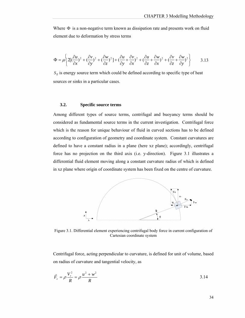
CHAPTER 3 Modelling Methodology
34
Where is a non-negative term known as dissipation rate and presents work on fluid
element due to deformation by stress terms
222222 )()()(])()()[(2y
w
z
v
x
w
z
u
x
v
y
u
z
w
y
v
x
u
3.13
ES is energy source term which could be defined according to specific type of heat
sources or sinks in a particular cases.
3.2. Specific source terms
Among different types of source terms, centrifugal and buoyancy terms should be
considered as fundamental source terms in the current investigation. Centrifugal force
which is the reason for unique behaviour of fluid in curved sections has to be defined
according to configuration of geometry and coordinate system. Constant curvatures are
defined to have a constant radius in a plane (here xz plane); accordingly, centrifugal
force has no projection on the third axis (i.e. y-direction). Figure 3.1 illustrates a
differential fluid element moving along a constant curvature radius of which is defined
in xz plane where origin of coordinate system has been fixed on the centre of curvature.
Figure 3.1. Differential element experiencing centrifugal body force in current configuration of Cartesian coordinate system
Centrifugal force, acting perpendicular to curvature, is defined for unit of volume, based
on radius of curvature and tangential velocity, as
R
wu
R
VF r
c
222
3.14
CHAPTER 3 Modelling Methodology
35
By replacing local value of R , sin and cos as 22 zx , 22 zx
z
and
22 zx
x
respectively, components of centrifugal force in x and z direction would be as
22
22
.coszx
wuxFF ccx
22
22
.sinzx
wuzFF ccz
3.15 (a)
3.15 (b)
It should be taken care to apply this source term just for curved section of domain (i.e.
0z ) and not for those straight inlet and outlet sections. This has been ensured by
including a sign function as follow
22
22
)(..zx
wuzsignxFcx
22
22
)(..zx
wuzsignzFcz
3.16 (a)
3.16 (b)
Buoyancy effect should be taken into account as well since this research investigates
mixed convection and interaction between centrifugal and buoyancy forces. This source
term, which acts in opposite direction of gravity, is induced by density difference due to
temperature gradient in flow field. The common solution which is usually utilized with
reasonable accuracy is linear Boussinesq assumption. This assumption linearly relates
pressure gradient along gravity direction with density difference [58, 59]. Nevertheless,
this model uses a higher order of temperature dependency and defines buoyancy force
as
]ˆˆˆ)[( kgjgigTF zyxb
3.17
3.3. Turbulence modelling
Fundamental conservation equations of mass and momentum are solely enough to
predict flow behaviour and temperature distribution for a laminar regime. However, by
increasing Reynolds number they would be inadequate to model random and chaotic
features of flow raised by turbulence. Reynolds Averaged Navier Stokes (RANS)
turbulent models have been developed assuming mean and fluctuating component for
flow velocity based on specific time and length scale proportional with eddies’ scale

CHAPTER 3 Modelling Methodology
36
[60]. Among wide range of turbulence models, two-equation models, which were first
introduced by Kolmogrov, are well established to have a reasonable competency for
prediction of such a flow characteristics. For current investigation proper turbulence
models has been designated with prospective of two concerns: first, accuracy of flow
inside the field and then, competency of wall treatment procedure. k and k
closures will be represented in the following chapters where both have been applied for
the specific case studies. However, turbulence modelling and its relevance to
conservation equation is generally explained here.
As it is mentioned, for a turbulent flow velocity has mean and fluctuating value defined
as 'uUu , 'vVv and 'wWw whereas similarly pressure would be defined as
'pPp . On ground of that turbulence kinetic energy could be formulated as
)'''(2
1 222 wvuk
3.18
and it would be related to turbulence intensity using reference velocity as
refT U
kI
21
)2
3(
3.19
Utilizing new obtained velocity and pressure terms into equation.3.11 and 3.12, they
would reformed into
bodyxfz
wu
y
vu
x
uU
x
P
z
UW
y
UV
x
UU
]'''''
[1 2
2
bodyyfz
wv
y
v
x
vuV
y
P
z
VW
y
VV
x
VU
]'''''
[1 2
2
bodyzfz
w
y
wv
x
wuW
z
P
z
WW
y
WV
x
WU
]'''''
[1 2
2
3.20 (a)
3.20 (b)
3.20 (c)
and
Ep
Sz
Tw
y
Tv
x
TuT
C
K
z
TW
y
TV
x
TU
]'''
[2
3.21
For more clarity Reynolds stress terms have been presented in term of fluctuating
velocities; however, these tensor notation of these terms is written as
CHAPTER 3 Modelling Methodology
37
)(i
j
j
itjiij x
U
x
Uuu
3.22
This stress terms which are key parameter for coupling turbulence and conservation
equations is defined according to applied turbulence model. Turbulence viscosity by
k model is defined as:
~
kt ,
*lim
2,max~
ijij SS
C , 8
7lim C 3.23
where
)(2
1
i
j
j
iij x
U
x
US
3.24
This key parameter is defined by k model as
2
0845.0k
t 3.25
3.4. Finite volume and Discretisation
Conservation equation for momentum, energy and turbulence are a set of partial
differential equation known as transport equation are to be numerically solved by of so
called Finite Volume method. This method which has been widely applied and
approved in for CFD method is quite well established; however, it should be taken into
account that crucial sub-procedure (e.g. discretisation, pressure-velocity coupling,
pressure correction) should be specifically set for each case. It basically takes advantage
of integrating transport equation over a differential control volume and then uses an
integral conversion to obtain the integral in surface form of that. Regardless of pressure
gradient term, effectiveness of which will later be taken into account by velocity-
pressure coupling formulation, a general form of a diffusive-convective transport
equation for general property of , where
is diffusion coefficient and S
is property
source term, would be as
SU )()( 2 3.26
which could be integrated over a control volume and then converted to a surface integral
over surfaces of given volume as
CHAPTER 3 Modelling Methodology
38
CVCVCV
dVSdVdVU )()( 2
CVAA
dVSdAndAUn )(.).(
3.27 (a)
3.27 (b)
Assuming a point of P at the centre of cubic differential control volume, known as cell,
which is neighboured with six other cells having centre points of E, W, S, N, T and B
respectively, representing west, east, south, north, top and bottom side of P,
equation.3.27-b could be rewritten in form of
VSx
Ax
A
xA
xA
xA
xA
AwAwAvAvAuAu
btt
ttt
sss
nnn
wWW
eee
btsnwe
)()()()()()(
3.28
Using neighbour cell values, gradient value are to be obtained and as the length scale is
assumed to be fine enough, it would be a consistent to assume linear variation for given
property respect to differential length and replace cell gradient values as:
VSz
Az
A
yA
yA
xA
xA
AwAwAvAvAuAu
tPB
BPtt
TP
PTtt
PS
SPss
NP
pnnn
PW
WPWW
EP
pEee
ttsnwe
)()()()()()(
3.29
Face values for convective term should be interpolated using neighbour cells values.
This procedure which is known as discretisation could be carried out using various
formulations such as central, upwind, hybrid and quick. Each method is assessed by
fundamental criteria of Conservativeness, Boundedness and Transportiveness, well
explained in literature. Upwind scheme has been chosen as an optimum method for
discretization as it is preferred, as compared to central scheme, for prediction of flow
direction where strong convection is involved [57]. Upwind differencing method (also
called “donor cell differencing scheme”) takes the direction of flow into account when
estimating value at cell face: the convective value ( u ) at cell face will be assumed to
be equal with upstream node value. Based on explained coordinate system (i.e. x-
CHAPTER 3 Modelling Methodology
39
positive East to West, y-positive South to North, z-positive Bottom to Top) Table.3.1
shows application upwind scheme for derivation of convective terms
Table 3.1. Application of upwind scheme for derivation of convective terms
eu )( wu )( sv )( nv )( bw )( tw )(
0u Eu )( Pu )( 0v Sv )( Pv )( 0w Bw )( Pw )(
0u pu )( Wu )( 0v Pv )( Nv )( 0w Pw )( Tw )(
In spite of good stability and consistency with transportiveness requirements for highly
convective field, such a formulation occasionally causes numerical error known as
“False diffusion”. Preventing such a problem and improving interpolation accuracy,
second order of upwind discritization could be utilized by which more neighbour nodes
will be involved and a wider influence will be taken into account (as it has been applied
for current study). Having the equation sorted according to P ,it would be possible to
use either explicit or implicit to solve the equation which will be a numerical policy
based on physics of problem, type of coupling and etc. However, for steady state
problem explicit approach is usually competent and fast enough and is recommended.
Second order upwind is preferred discretisation in most cases in this study and so is
explained briefly; nevertheless, in some cases (specially for the purpose of multi-phase
modelling) other schemes have been used which will be just pointed in the relevant
parts.
3.5. Pressure-velocity Coupling, pressure correction and residual
Since generalized form of transport equation does not include pressure gradient term
which is a crucial term of momentum equation, direct solution of this form of equation
cannot obtain correct velocity field. Among different available algorithm, SIMPLE
(Semi-Implicit Method for Pressure Linked Equations) has been chosen for single phase
simulation where it basically uses a staggered grid which has different nodes for scalar
and velocity values. Using initial guess fields (i.e. **** ,,, pwvu ) and finite volume
formulation, uncorrected velocities ( ',',' wvu ) would be first obtained. Then, so called
CHAPTER 3 Modelling Methodology
40
pressure correction equation will be solved to obtain 'p where pressure interpolation
would be necessary to discretise such equation. Finally by the key approximation of
SIMPLE algorithm, corrected pressure is used to obtain corrected velocities and this
iterative procedure would be continued until convergence achievement.
In presence of large body forces and strongly swirling, it is necessary either to pack the
mesh in regions of high gradient to resolve the pressure variation adequately or to use
alternative interpolation scheme such as body force weighted which has been utilized
here. The body-force-weighted scheme computes the face pressure by assuming that
the normal gradient of the difference between pressure and body forces is constant.
There are different policies as convergence criteria such as classic absolute and relative
error approach which explicitly compares results from current iteration with the
previous one and on such basis judges about convergence. Applied solver, however,
uses another method based on computed residual term for transport equation and could
be utilized both globally and locally. “Globally scaled” residual term for applied solver
is defined as:
Cells
npp
Cells
npp
nbnbnb
a
aba
R
1
1
3.30
where “p” and “nb” subscripts represent centre and neighbour cell values and
coefficients. This residual could also be defined “locally scaled” as:
domain
Cells
n p
ppnb
nbnb
a
aba
n
R)(
1
minmax
1
3.31
Moreover, consistency of mass transfer between inlet and outlet is monitored for all
cases as well as some other local monitoring if required which will be discussed in
relevant part.
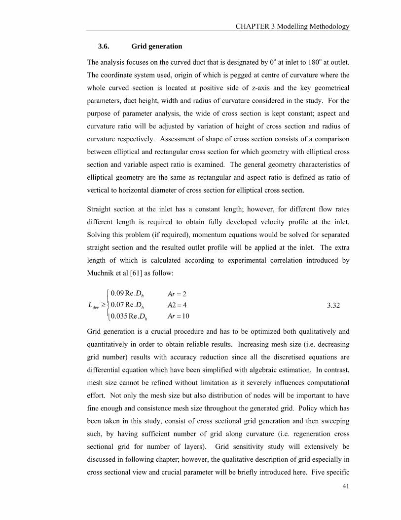
CHAPTER 3 Modelling Methodology
41
3.6. Grid generation
The analysis focuses on the curved duct that is designated by 0o at inlet to 180o at outlet.
The coordinate system used, origin of which is pegged at centre of curvature where the
whole curved section is located at positive side of z-axis and the key geometrical
parameters, duct height, width and radius of curvature considered in the study. For the
purpose of parameter analysis, the wide of cross section is kept constant; aspect and
curvature ratio will be adjusted by variation of height of cross section and radius of
curvature respectively. Assessment of shape of cross section consists of a comparison
between elliptical and rectangular cross section for which geometry with elliptical cross
section and variable aspect ratio is examined. The general geometry characteristics of
elliptical geometry are the same as rectangular and aspect ratio is defined as ratio of
vertical to horizontal diameter of cross section for elliptical cross section.
Straight section at the inlet has a constant length; however, for different flow rates
different length is required to obtain fully developed velocity profile at the inlet.
Solving this problem (if required), momentum equations would be solved for separated
straight section and the resulted outlet profile will be applied at the inlet. The extra
length of which is calculated according to experimental correlation introduced by
Muchnik et al [61] as follow:
h
h
h
dev
D
D
D
L
.Re035.0
.Re07.0
.Re09.0
10
42
2
Ar
A
Ar
3.32
Grid generation is a crucial procedure and has to be optimized both qualitatively and
quantitatively in order to obtain reliable results. Increasing mesh size (i.e. decreasing
grid number) results with accuracy reduction since all the discretised equations are
differential equation which have been simplified with algebraic estimation. In contrast,
mesh size cannot be refined without limitation as it severely influences computational
effort. Not only the mesh size but also distribution of nodes will be important to have
fine enough and consistence mesh size throughout the generated grid. Policy which has
been taken in this study, consist of cross sectional grid generation and then sweeping
such, by having sufficient number of grid along curvature (i.e. regeneration cross
sectional grid for number of layers). Grid sensitivity study will extensively be
discussed in following chapter; however, the qualitative description of grid especially in
cross sectional view and crucial parameter will be briefly introduced here. Five specific

CHAPTER 3 Modelling Methodology
42
concerns in case of curved channel have to be taken into account for proper grid
generation:
Adequate number of grid is required in all three-dimensions (i.e. horizontal,
vertical and axial direction) which could be obtained through grid sensitivity
analysis.
For both rectangular and elliptical cross sections structure mesh is preferred in
order to reduce effect of False-diffusion and reducing computational effort.
Achieving such a requirement the elliptical cross sections should be meshed as a
multi-zone plane which will be explained in details in following sections.
For single-phase instability analysis pressure-gradient should be grid
independent on the outer wall; for such a purpose mesh should be compacted
toward outer wall.
For multi-phase instability analysis due to relocation of different phases next to
inner and outer walls, mesh should be compacted toward both inner wall and
outer wall.
For turbulent cases, the mesh should be refined in order to obtain consistence y
value obeying requirement of model and solver (i.e. 5y for k model and
30030 y for k model)
Figure 3.2. illustrates samples of mesh in cross sectional and axial views obeying
explained confinements. As an example, Figure 3.2 (a) is depicting a grid which could
be used for investigation of Dean instability in single phase domain; however, for two-
phase investigation as it was mentioned grid should be compacted toward inner wall as
well as outer wall which turns it to what is shown in Figure 3.2 (b). Mesh sweeping in
axial direction is not so critical and nodes are distributed uniformly as a part of curved
section is shown in Figure 3.2 (b); yet, number of nodes should be optimized with grid
sensitivity examination.
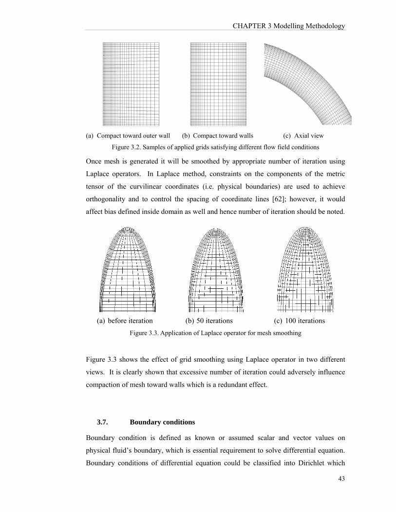
CHAPTER 3 Modelling Methodology
43
(a) Compact toward outer wall (b) Compact toward walls (c) Axial view
Figure 3.2. Samples of applied grids satisfying different flow field conditions
Once mesh is generated it will be smoothed by appropriate number of iteration using
Laplace operators. In Laplace method, constraints on the components of the metric
tensor of the curvilinear coordinates (i.e. physical boundaries) are used to achieve
orthogonality and to control the spacing of coordinate lines [62]; however, it would
affect bias defined inside domain as well and hence number of iteration should be noted.
(a) before iteration (b) 50 iterations (c) 100 iterations
Figure 3.3. Application of Laplace operator for mesh smoothing
Figure 3.3 shows the effect of grid smoothing using Laplace operator in two different
views. It is clearly shown that excessive number of iteration could adversely influence
compaction of mesh toward walls which is a redundant effect.
3.7. Boundary conditions
Boundary condition is defined as known or assumed scalar and vector values on
physical fluid’s boundary, which is essential requirement to solve differential equation.
Boundary conditions of differential equation could be classified into Dirichlet which
CHAPTER 3 Modelling Methodology
44
assumes constant value on the given boundary (i.e. tcons tan ) or Neumann which
assumes constant gradient (i.e. tconsxi
tan ). Nevertheless, it should be noted that
unlike a purely mathematical problem, while these equation are used to model a
physical phenomenon, boundary condition assumption should be physically valid; so
that, there are a series of limitation according which boundary conditions should be
applied precisely. Current model consists of three types of physical boundaries: inlet,
outlet and solid wall which will be adjusted according to physics of fluid (e.g.
single/multi-phase, laminar/turbulence flow) or applied numerical model (e.g. k /
k model).
a) Inlet
Velocity inlet: this type of boundary condition which is here used for both single
and multi-phase analysis, assumes velocity at inlet to be function of position.
For sake of having a fully developed velocity profile, in most cases inlet velocity
profile has been extracted form an inlet straight section. Other scalars including
temperature (Tin=Constant=300 ̊K), turbulence kinetic energy ( k ), turbulence
dissipation rate ( ) and specific dissipation rate ( ) could be defined as either
constant or function of position by an input profile. For an incompressible fluid
this type of boundary condition is the same as mass flow rate boundary
condition.
b) Outlet
Outflow: this type of boundary condition is used when the outlet condition is
almost unknown and fields such as pressure and velocity are left to be computed
by solver. It should be seriously taken care to have fairly fully developed
velocity and temperature fields at the outlet while using this boundary condition.
The reason for this confinement is all gradients will be assumed to be constant
normal to such boundary by definition; hence, if the field is not fully developed
field will introduce an error into domain from the outlet boundary. Having the
outlet passage section in the geometry will guarantee a confident application of
outflow boundary condition for single-phase model as a robust boundary
accelerating convergence. However, due to modelling limitation and due to lack
of development conditions for VOF and Mixture model at the outlet this

CHAPTER 3 Modelling Methodology
45
boundary is not the best choice there and it was replaced with a pressure-outlet
boundary.
Pressure outlet: Using this type of boundary condition fully development
confinement will be eliminated and by which occurrence of back-flow will be
possible. Defined pressure at the outlet will be gauge pressure. It could be used
especially if the pressure drop inside the channel is known.
c) Wall
No slip boundary condition: possibly the most common solid boundaries
assumption which consider fluid velocity to be the same as solid wall velocity in
adjacent of that. Accordingly flow will have zero velocity next to stationary
wall.
Isothermal boundary condition: fluid temperature is the same as solid wall in
adjacent of that. This type of boundary condition has been used for both single
and multi-phase models.
Constant heat flux: temperature gradient on the solid surface in normal direction
( tconsn
T
n
tan0
) should be kept constant to have constant heat flux. This type
of boundary condition has been used for both single and multi-phase models.
Turbulence model near wall treatment: as it was mentioned in turbulence
modelling part, estimation of fluid behaviour in sub-layer, defect-layer and log
layer referred as wall treatment significantly affects investigation of parameters
such as wall shear stress or pressure gradient. Generally explaining, k model
solves sub-layer whereas model k estimate it using an algebraic equation.
Considering solver (i.e. FLUENT) and model requirement for current model,
turbulence dimensionless distance from wall should be taken care to satisfy
5y and 30030 y for k and k respectively in order to have
consistent turbulence results.
3.8. Multi-phase flow modelling
A multi-phase numerical model calculates velocity and other scalar properties of fluids
and to track phase interfaces. Different multi-phase models are available which could
CHAPTER 3 Modelling Methodology
46
be used according to type of flow, limitation and requirements. The most common
multi-phase models, which are available in applied commercial packages, are VOF
(Volume Of Fraction), Mixture and Eulerian models each of them has competencies and
limitations. VOF and Mixture models both solve a single set of transport equation for
all phases whereas Eulerian model solves it for each phase separately. VOF and
Eulerian method have been used respectively for immiscible flow (where just
momentum is being transferred between phases) and boiling case (where mass diffusion
through phase interface is additionally taken into account). As it first pointed, the most
crucial challenge in multi-phase modelling is recognition of phase interfaces for which a
new concept is introduced known as “volume of fraction” and represented by . This
scalar identifies volume of cell which is occupied with a given fluid. As an instant for
fluid referred by ""W , volume fraction of W represents:
0W : cell is empty of given fluid
1W : cell is full of given fluid
10 W : cell is located on boundary of fluids and partially is filled with
given flow
Referring “volume fraction” definition, it is summarized that 11
n
pp . This statement
in addition with continuity equation which takes volume fraction into account,
accomplish interface tracking. Continuity equation however, is solved separately for
each phase to obtain volume of fraction which is also used for calculation of material
properties as well. For phase-q, continuity equation in steady form is written as:
n
pqppqqqq
q
mmV1
)().(1
3.33
In this equation, pqm is mass transfer from phase-p to phase q and qpm is mass transfer
from phase-q to phase-p. By obtaining volume fraction, it would be initially possible to
calculate material properties as bulk values in cells placed on the interfaces. Every
scalar will be calculated according to each material properties and given volume
fraction as:
n
ppp
1
3.34
CHAPTER 3 Modelling Methodology
47
Properties such as density, viscosity, thermal conductivity and specific heat capacity are
calculated according to such formulation and will be used in momentum and energy
equation which are solved throughout domain for all the phases. This forms the
simplest yet competent methodology for interface tracking and multi-phase flow
analysis which is known as VOF. However, these equations are to be numerically
solved by finite volume approach previously mentioned. For discritization and
interpolation procedure, explained schemes (e.g. central, upwind, quick) are available
for multi-phase as well; yet, interpolation on the interfaces is a specific concern which
affects not only on cell values but also on shape of interface. Donor-acceptor and
geometry-reconstruction method are introduced as the most sophisticated approaches
for interface interpolation [63].
In cells close to phase interfaces, "donor-acceptor'' scheme is used to determine the
amount of fluid advected through the face where for rest of cells having volume fraction
of one, standard interpolation scheme is used. This scheme identifies one cell as a
donor of fluid from one phase and another (neighbor) cell as the acceptor of that same
amount of fluid. The amount of fluid from one phase that can be convected across a cell
boundary is limited by the minimum of two values: the filled volume in the donor cell
or the free volume in the acceptor cell [64]. In this approach phase interface in each cell
could be either vertical or horizontal according to direction of volume fraction gradient.
Geo-reconstruction scheme is another precise interpolation method which is specifically
suggested for interface interpolation in multi-phase domains. Geo-reconstruction
scheme represents the interface between fluids using a piecewise-linear approach and
generalized for unstructured grids assuming the interface between two fluids has a linear
slope within each cell. Position of the linear interface relative to the center of each
partially-filled cell is calculated, based on information about the volume fraction and its
derivatives in the cell. Surface tension which is raised as a result of attractive force
between molecules is another important parameter and could be related to pressure jump
(i.e. pressure difference between phases) on boundaries. It is calculated based on
contact angle of two phases and surface tension coefficient which could be dependent to
temperature. Although surface tension has a well-established and simple formulation it
should be noted that avoiding numerical instability pressure does not jump from one cell
to the neighbour cells and so the phase boundary does not have a distinct recognition
and depend on model is a strip or fine volume. Developing VOF model, level-set model
has been recently introduced which helps to capture and track sharp interfaces
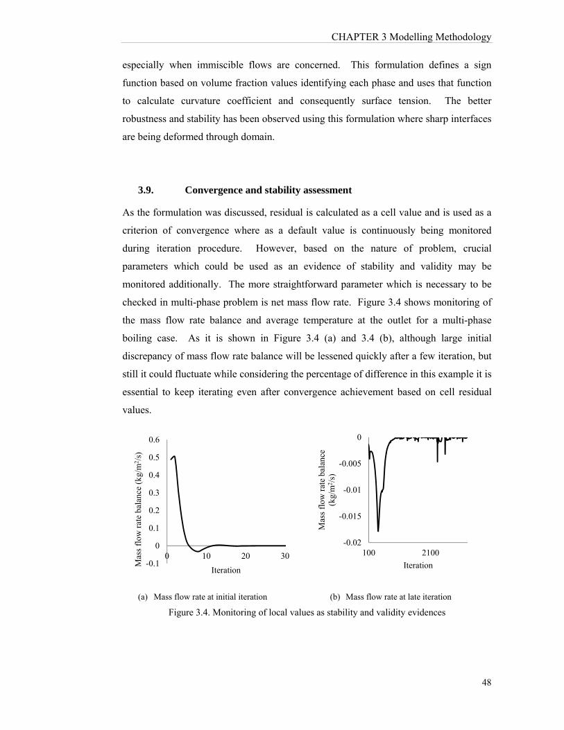
CHAPTER 3 Modelling Methodology
48
especially when immiscible flows are concerned. This formulation defines a sign
function based on volume fraction values identifying each phase and uses that function
to calculate curvature coefficient and consequently surface tension. The better
robustness and stability has been observed using this formulation where sharp interfaces
are being deformed through domain.
3.9. Convergence and stability assessment
As the formulation was discussed, residual is calculated as a cell value and is used as a
criterion of convergence where as a default value is continuously being monitored
during iteration procedure. However, based on the nature of problem, crucial
parameters which could be used as an evidence of stability and validity may be
monitored additionally. The more straightforward parameter which is necessary to be
checked in multi-phase problem is net mass flow rate. Figure 3.4 shows monitoring of
the mass flow rate balance and average temperature at the outlet for a multi-phase
boiling case. As it is shown in Figure 3.4 (a) and 3.4 (b), although large initial
discrepancy of mass flow rate balance will be lessened quickly after a few iteration, but
still it could fluctuate while considering the percentage of difference in this example it is
essential to keep iterating even after convergence achievement based on cell residual
values.
(a) Mass flow rate at initial iteration (b) Mass flow rate at late iteration
Figure 3.4. Monitoring of local values as stability and validity evidences
-0.1
0
0.1
0.2
0.3
0.4
0.5
0.6
0 10 20 30
Mas
s fl
ow r
ate
bala
nce
(kg/
m2 /
s)
Iteration
-0.02
-0.015
-0.01
-0.005
0
100 2100
Mas
s fl
ow r
ate
bala
nce
(kg/
m2 /
s)
Iteration
CHAPTER 3 Modelling Methodology
49
3.10. Summary
In this chapter general guidelines of CFD methodology, valid for all case studies in this
research, have been explained. Three different numerical models will be developed,
explained and utilized in following chapters on the basis of this methodology either of
them has specific modelling and validation concerns. Governing equation, boundary
condition configuration and validation criteria will be discussed for each model
separately.

CHAPTER 4 Single-Phase Flow and Heat Transfer in Curved Channels
50
CHAPTER 4
CHAPTER 4 Single-Phase Flow and Heat Transfer in Curved Channels
4.1. Scope of Chapter
Reviewing published numerical and experimental work, this chapter discusses the
current knowledge-base on secondary flow in curved ducts and, identifies the
deficiencies in analyses and fundamental understanding. It then presents an extensive
research study capturing advanced aspects of secondary flow behaviour and associated
wall heat transfer processes for both rectangular and elliptical ducts.
Overcoming current limitations, the study develops a new three-dimensional numerical
model incorporating helicity approach that is validated against published data. Flow
patterns and thermal characteristics are obtained for a range of duct aspect ratios, flow
rates and wall heat fluxes. Results are analysed for parametric influences and construed
for clearer physical understanding of the flow mechanics involved. The study
formulates two analytical techniques whereby secondary vortex detection is integrated
into the computational process with unprecedented accuracy and reliability. The vortex
inception at flow instability is carefully examined with respect to the duct aspect ratio,
duct geometry and flow rate. An entropy-based thermal optimisation technique is
developed and tested for fluid flow through curved rectangular and elliptical ducts.
4.2. Introduction
The centrifugal action induced by duct curvature imparts two key effects on the fluid
flow. It produces a lateral fluid movement directed from inner duct wall towards the
outer wall in the axial flow, thus causing a spiralling fluid motion through the duct.
This lateral fluid movement is manifested by large counter rotating pairs of vortices
appearing in the duct cross section and is referred to as secondary flow. The centrifugal
action also forms a radial fluid pressure gradient positively biased towards the outer
CHAPTER 4 Single-Phase Flow and Heat Transfer in Curved Channels
51
duct wall. The lateral fluid circulation takes place adversely to the radial pressure field
and is dampened by the viscous effects. The combined actions of positive radial
pressure gradient and viscous forces form a stagnant fluid region near the outer wall.
Beyond a certain critical axial flow rate, the radial pressure gradient would exceed the
equilibrium condition in the stagnant fluid region at outer wall and triggers a localised
flow circulation to form additional pairs of vortices. This flow condition is known as
Dean Instability [5] and the additional vortices are called Dean Vortices.
Most experimental and numerical analyses on curved ducts have been performed on
rectangular duct geometries. By virtue of shape, such ducts have less wall interference
on secondary vortex formation making it relatively easier for numerical modelling and
convenient for experimentation including flow visualisation. Ducts with elliptical and
circular cross sections have received less research attention in spite of being a common
geometry used in most technological systems and, remain relatively unexplored.
Above scrutiny of published literature indicates that the available modelling methods
have yet to develop for realistic representation of complex secondary flow behaviour
and improved predictability for Dean Instability. Parametric influences of duct
geometry and flow variables remain unexplored and poorly understood with no decisive
approach for defining the onset of Dean vortices and their locations. Significantly
improving these shortfalls, this chapter describes an advanced three-dimensional
numerical simulation methodology based on helicity, which is congruent with the
vortex motion of secondary flow. Facilitating much compliant tracking of vortex flow
paths, the model uses a curvilinear mesh that is more effective in capturing the intricate
details of vortices with the advantage of being applicable for both rectangular and
elliptical ducts. Two intuitive approaches for detecting the onset of Dean Instability are
proposed and tested in the study. An extensive parametric investigation is presented
with physical interpretation of results for improved understanding of flow behaviour. A
thermal optimisation scheme based on flow irreversibilities is developed and
demonstrated for curved ducts.
4.3. Numerical model
4.3.1 Geometry and boundary conditions
Figure 4.1 shows the rectangular and elliptical duct geometries used for the three-
dimensional simulation model in the current study. It also indicates the key geometrical
parameters, duct height a, width b and the radius of curvature R. The geometrical
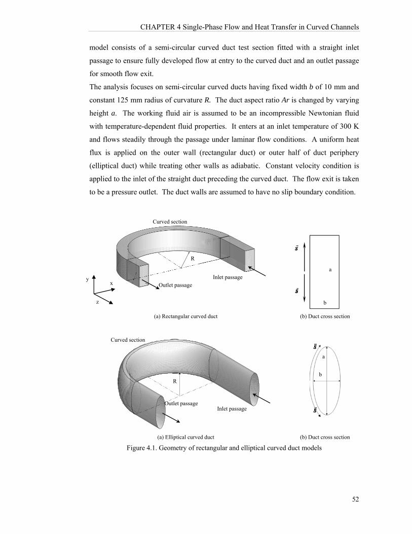
CHAPTER 4 Single-Phase Flow and Heat Transfer in Curved Channels
52
model consists of a semi-circular curved duct test section fitted with a straight inlet
passage to ensure fully developed flow at entry to the curved duct and an outlet passage
for smooth flow exit.
The analysis focuses on semi-circular curved ducts having fixed width b of 10 mm and
constant 125 mm radius of curvature R. The duct aspect ratio Ar is changed by varying
height a. The working fluid air is assumed to be an incompressible Newtonian fluid
with temperature-dependent fluid properties. It enters at an inlet temperature of 300 K
and flows steadily through the passage under laminar flow conditions. A uniform heat
flux is applied on the outer wall (rectangular duct) or outer half of duct periphery
(elliptical duct) while treating other walls as adiabatic. Constant velocity condition is
applied to the inlet of the straight duct preceding the curved duct. The flow exit is taken
to be a pressure outlet. The duct walls are assumed to have no slip boundary condition.
(a) Rectangular curved duct (b) Duct cross section
(a) Elliptical curved duct (b) Duct cross section
Figure 4.1. Geometry of rectangular and elliptical curved duct models
a
b
x
z
y
Curved section
Inlet passage Outlet passage
R
Curved section
Inlet passage
R
Outlet passage
b
a

CHAPTER 4 Single-Phase Flow and Heat Transfer in Curved Channels
53
4.3.2 Governing equations
Equation should be derived for an incompressible, laminar steady flow with centrifugal
force as specific momentum source term. As a result of heating and temperature
gradient in the domain, buoyancy source term should be taken into account as well.
The numerical model solves the following governing equations:
Time-averaged continuity equation:
0).( V
4.1
the momentum and energy conservation equations:
cm FgVpVV
2)(. 4.2(a)
Tp STkTcV 2)(.
4.2(b)
The magnitude of the centrifugal body force term in radial direction is given by,
22
222 )(
zx
wu
r
VF r
c
4.3
Considering the position and alignment of curved part of geometry, centrifugal source
term in Cartesian coordinate system is obtained from,
)ˆˆ()(
2
)(122
22
kzixzx
wuzsignFc
4.4
In Equation 4, a Sign Function is used to ensure the centrifugal source term is applied
only on the curved side of the geometry (i.e. z 0). For obtaining the dimensionless
parameters, the characteristics length, velocity and pressure are chosen to be , ,
, respectively.
The thermally-induced buoyancy is included in the model by relating the density m in
Equation. 4.2 (a) to local fluid temperature. For this, a sixth-order polynomial as given
by Equation.4.5 is developed, where the given polynomial is defined according to NIST
standard reference database (webBook). This order of polynomial is essential to capture
behaviour of fluid at very high temperature and to achieve R-square value larger than
0.995”. This approach is necessary because the linearity of the Boussinesq
approximation caused some discrepancy and is found to be inadequate for evaluating
the wall pressure gradient.
CHAPTER 4 Single-Phase Flow and Heat Transfer in Curved Channels
54
3618.91008.0
10610210310310)( 443649512615
T
TTTTTT 4.5
In capturing the helix-like fluid motion of secondary flow, this three-dimensional model
incorporates a helicity function, which is defined by Equation.4.6. The helicity is non-
dimensionalised using the reference helicity based on hydraulic diameter, as given by
Equation.4.7.
)()()(.y
u
x
vw
x
w
z
uv
z
v
y
wuVH
4.6
)(2
*2
in
h
h
in
U
DHH
D
UH 4.7
For identifying the onset of Dean instability, the model proposes two separate criteria.
The first criterion is based on helicity, which is computed from Equation.4.7. The
second criterion uses the outer duct wall pressure gradient profile for which the non-
dimensional wall pressure gradient is obtained from Equation.4.8. A sign convention is
incorporated in Equation.4.8 to designate the opposite rotational directions of the
vortices in upper and lower half of duct cross section, following the selection of
coordinate along the outer wall of duct cross section, as depicted in Figure 1 (b).
For the forced convective heat transfer in the duct, the local Nusselt Number is defined
as k
hDNu where the heat transfer coefficient h, is determined by considering the grid
cell temperature difference between the heated wall and the adjacent fluid cell. The
average Nusselt number is obtained from the surface integral, A
NudA
uN A
.
The model formulates a thermal optimisation scheme using flow irreversibility as a
criterion. For this, the overall entropy generation split in to the components of
irreversibility contributed by the wall heat transfer, including thermally-induced
buoyancy effects and, that due to fluid flow friction compounded by secondary fluid
motion. As such, the components of entropy generation from heat transfer (S ) and that
ds
dp
U
D
ds
dp
U
D
Sd
dp
in
h
in
h
2
2*
21
21
at lower half of cross section
at upper half of cross section
4.8
CHAPTER 4 Single-Phase Flow and Heat Transfer in Curved Channels
55
from fluid friction (S ) within the solution domain are evaluated using the expressions
4.9 (a), (b) and (c).
2222
)()()(z
T
y
T
x
T
T
kST 4.9(a)
T
SP
4.9(b)
where,
222222 )()()(])()()[(2x
w
z
u
z
v
y
w
x
v
y
u
z
w
y
v
x
u
4.9(c)
The entropy terms are generalised as volumetric-averaged values using,
dv
dvSS
T
T 4.10(a)
dv
dvSS
p
p
4.10(b)
pTg SSS
4.10(c)
Based on the above volumetric entropy generation terms, Bejan number is defined as,
g
T
S
SBe
4.11
Bejan Number reflects the relative domination of flow irreversibility by heat transfer
with respect to the overall irreversibility [65]. In this, magnitude 1 for Bejan Number
indicates totally heat transfer-dominated entropy generation while 0 refers to fluid
friction causing all of flow irreversibility. Thus for curved ducts, the Bejan number
performs as a visual map signifying the relative strength of thermal effects within the
fluid domain interacted by the secondary flow and Dean vortices. This approach is then
utilised for thermally optimising the forced convection process in ducts.
Incorporating above governing equations, a finite volume-based CFD model is
formulated with the commercial package FLUENT where SIMPLE algorithm is used
for pressure-velocity coupling. The momentum and energy equations are discretised by
first and second order schemes, respectively. Since the model considers both buoyancy
and centrifugal source terms, pressure discretisation is performed with body force-
weighted approach. The stability of the solution is monitored through continuity,
velocity, energy and dimensionless helicty where the convergence is achieved with
values not higher than 10-5. Grid independency is carefully checked paying a special
attention to boundary layer modelling at the outer wall.

CHAPTER 4 Single-Phase Flow and Heat Transfer in Curved Channels
56
The simulation is performed to obtain the profiles of velocity, helicity, temperature and
Bejan Number at curved duct for a range of flow rates giving Dean Number within 80
to 1600. The wall heat flux is varied up to 4000 W/m2. The results showing some signs
of Dean vortices are further refined by re-running the simulations with closer steps of K
to determine the exact point of instability and the critical Dean number. This procedure
is repeated for all aspect ratios, flow rates and heat fluxes. Forced convection is
evaluated by the local and average Nusselt numbers at the duct wall.
4.3.3 Grid sensitivity and Model Validation
In secondary flow simulations, the solution convergence is critically dependent on the
grid selection because of the intricate flow patterns and intense flow gradients. For
rectangular ducts, a single-zone mesh would be adequate. However, due to the
geometrical shape, elliptical ducts have much extreme flow field gradients and would
require a more stringent grid arrangement.
In rectangular ducts a progressively reducing mesh is used with a much finer mesh near
the outer wall where the onset of Dean Instability is anticipated. This approach has not
been attempted in previous studies [13, 15, 17] wherein it was argued that a mesh size
less than 1 mm would not improve accuracy, but only to increase computational time.
The mesh refinement of the present analysis clearly identifies that a finer mesh near the
wall is critical for detecting the onset of Dean vortices as accurately as possible. For
testing grid dependency, the study uses five mesh schemes indicated in Table 1. In this,
columns A, B and C represent the number of grids over duct width, height and length,
respectively, while the column D indicates the progressive reduction of grid size over
duct width towards the outer wall.
Table 2. Grid selection and mesh schemes for rectangular ducts
Scheme Number of Grids
A B C D
Mesh1 26 51 305 1
Mesh2 31 64 305 1
Mesh3 43 84 305 1
Mesh4 50 98 305 1
Mesh5 26 51 305 1.05
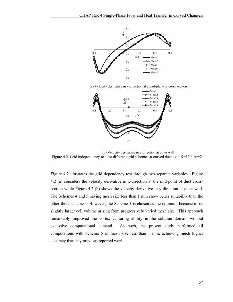
CHAPTER 4 Single-Phase Flow and Heat Transfer in Curved Channels
57
(a) Velocity derivative in x-direction at a mid-plane in cross section
(b) Velocity derivative in y-direction at outer wall Figure 4.2. Grid independency test for different grid schemes at curved duct exit, K=130, Ar=2
Figure 4.2 illustrates the grid dependency test through two separate variables. Figure
4.2 (a) considers the velocity derivative in x-direction at the mid-point of duct cross-
section while Figure 4.2 (b) shows the velocity derivative in y-direction at outer wall.
The Schemes 4 and 5 having mesh size less than 1 mm show better suitability than the
other three schemes. However, the Scheme 5 is chosen as the optimum because of its
slightly larger cell volume arising from progressively varied mesh size. This approach
remarkably improved the vortex capturing ability in the solution domain without
excessive computational demand. As such, the present study performed all
computations with Scheme 5 of mesh size less than 1 mm, achieving much higher
accuracy than any previous reported work.
-3.5
-2.5
-1.5
-0.5
0.5
1.5
2.5
-0.5 -0.3 -0.1 0.1 0.3 0.5
du/d
x
x/b Mesh1Mesh2Mesh3Mesh4Mesh5
-2
-1.5
-1
-0.5
0
0.5
1
-0.5 -0.3 -0.1 0.1 0.3 0.5
du/d
x
y/a
Mesh1Mesh2Mesh3Mesh4Mesh5
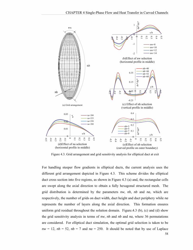
CHAPTER 4 Single-Phase Flow and Heat Transfer in Curved Channels
58
(a) Grid arrangement
(b)Effect of nw selection (horizontal profile in middle)
(c) Effect of nh selection
(vertical profile in middle)
(d)Effect of na selection (horizontal profile in middle)
(e)Effect of nb selection (curved profile on outer boundary)
Figure 4.3. Grid arrangement and grid sensitivity analysis for elliptical duct at exit
For handling steeper flow gradients in elliptical ducts, the current analysis uses the
different grid arrangement depicted in Figure 4.3. This scheme divides the elliptical
duct cross section into five regions, as shown in Figure 4.3 (a) and, the rectangular cells
are swept along the axial direction to obtain a fully hexagonal structured mesh. The
grid distribution is determined by the parameters nw, nh, nb and na, which are
respectively, the number of grids on duct width, duct height and duct periphery while na
represents the number of layers along the axial direction. This formation ensures
uniform grid residual throughout the solution domain. Figure.4.3 (b), (c) and (d) show
the grid sensitivity analysis in terms of nw, nh and nb and na, where 36 permutations
are considered. For elliptical duct simulation, the optimal grid selection is taken to be
nw = 12, nh = 52, nb = 7 and na = 250. It should be noted that by use of Laplace
-2
-1
0
1
-0.5
-0.4
-0.3
-0.2
-0.1
0 0.1
0.2
0.3
0.4
0.5
du*/
dx*
x/b
nw=8nw=10nw=12nw=14
-0.25
-0.05
0.15
0.35
-0.5
-0.4
-0.3
-0.2
-0.1
0 0.1
0.2
0.3
0.4
0.5
dv*/
dy*
y/b
nh=40nh=44nh=52nh=60
0
0.01
0.02
0.03
-0.5
-0.4
-0.3
-0.2
-0.1
0 0.1
0.2
0.3
0.4
0.5
w*
x/b
na=200
na=225
na=250
na=280
0
0.1
0.2
0.3
0.4
-0.5
-0.4
-0.3
-0.2
-0.1
0 0.1
0.2
0.3
0.4
0.5
dz*/
dz*
y/b
nb=3nb=5nb=7nb=9
CHAPTER 4 Single-Phase Flow and Heat Transfer in Curved Channels
59
operation, previously mentioned in section 3.6, good orthogonal and aspect ratio quality
is guaranteed on the border of zones.
For the purpose of validating results against published work, Figure 4.4 shows the axial
flow velocity in x and y directions predicted by the current 3-dimensional model and
those from the analyses of Ghia and Shokhey [10] and Fellouah et al [15], for
rectangular cross section. It is seen that both magnitudes and trends of axial velocity are
very favourably compared confirming the integrity of the numerical process.
Figure 4.4 also illustrates the secondary flow effect on the axial fluid velocity in the
curved passage. The profile on the left (along x axis) shows a skewed peak towards the
outer wall arising from the centrifugal action and is characteristically different to axial
velocity distribution in straight ducts. This peak gradually spreads towards the centre
with increasing flow rate because of the radial pressure build at the outer wall. The
profile on the right (along y axis) shows a dip in the centre and two marginal peaks on
other side. These peaks essentially correspond to the upper and lower “eye” of
secondary vortices. Increased flow rate shows a marginal impact on the profile.
Similarly for an elliptical duct, Figure 4.5 provides a comparison of the axial velocity
profiles at the mid cross section planes from the current study with those from Dong and
Ebadian [13] and Silva et al. [26]. A very good agreement is clearly evident validating
the numerical consistency of the present simulation.
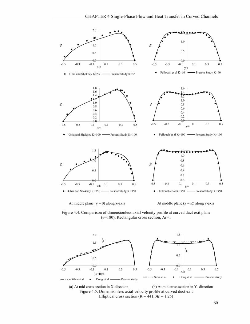
CHAPTER 4 Single-Phase Flow and Heat Transfer in Curved Channels
60
At middle plane (y = 0) along x-axis At middle plane (x = R) along y-axis
Figure 4.4. Comparison of dimensionless axial velocity profile at curved duct exit plane (θ=180̊), Rectangular cross section, Ar=1
(a) At mid cross section in X-direction (b) At mid cross section in Y- direction Figure 4.5. Dimensionless axial velocity profile at curved duct exit
Elliptical cross section (K = 441, Ar = 1.25)
0.0
0.5
1.0
1.5
2.0
-0.5 -0.3 -0.1 0.1 0.3 0.5V
r
x/b
Ghia and Shokhey K=55 Present Study K=55
0.0
0.5
1.0
1.5
-0.5 -0.3 -0.1 0.1 0.3 0.5
Vr
y/a
Fellouah et al K=60 Present Study K=60
0.00.20.40.60.81.01.21.41.61.8
-0.5 -0.3 -0.1 0.1 0.3 0.5
Vr
x/b
Ghia and Shokhey K=100 Present Study K=100
0.00.20.40.60.81.01.21.41.6
-0.5 -0.3 -0.1 0.1 0.3 0.5
Vr
y/a
Fellouah et al K=100 Present Study K=100
0.0
0.5
1.0
1.5
-0.5 -0.3 -0.1 0.1 0.3 0.5
Vr
x/b
Ghia and Shokhey K=350 Present Study K=350
0.0
0.2
0.4
0.6
0.8
1.0
1.2
-0.5 -0.3 -0.1 0.1 0.3 0.5
Vr
y/a
Fellouah et al K=350 Present Study K=350
0.0
0.5
1.0
1.5
2.0
-0.5 -0.3 -0.1 0.1 0.3 0.5
W*
(-x+R)/b
Silva et al Dong et al Present study
0.0
0.5
1.0
1.5
-0.5 -0.3 -0.1 0.1 0.3 0.5
W*
y/a
Silva et al Dong et al Present study
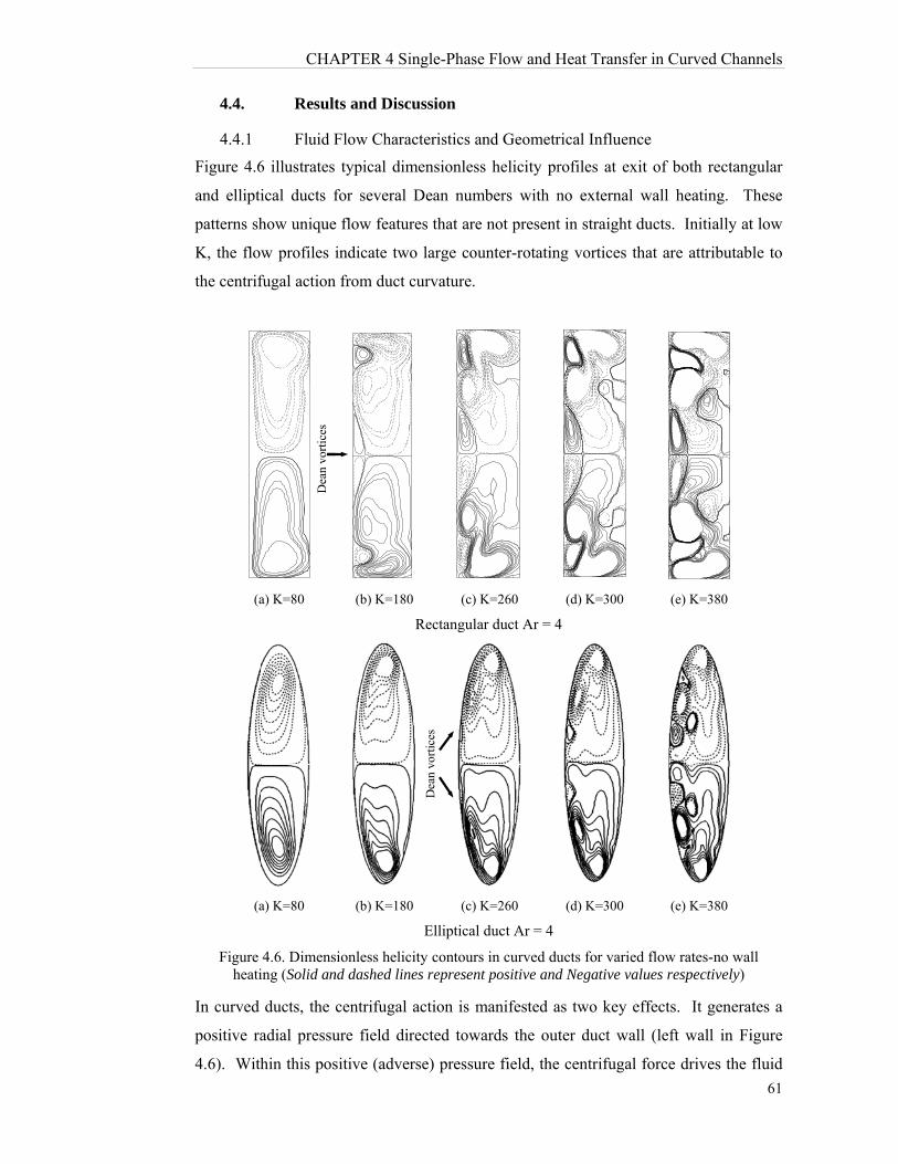
4.4.
4.4.1
Figure 4.6
and ellipti
patterns sh
K, the flow
the centrif
(a
(a
Figure heati
In curved
positive ra
4.6). With
CHA
Result
Fluid F
6 illustrates
ical ducts f
how unique
w profiles i
fugal action
a) K=80
a) K=80
4.6. Dimensing (Solid an
ducts, the
adial pressu
hin this pos
Dea
n vo
rtic
es
APTER 4 Si
ts and Disc
Flow Chara
typical dim
for several
e flow featur
indicate tw
n from duct c
(b) K=180
(b) K=180
sionless helicnd dashed lin
centrifugal
ure field dir
sitive (adve
ingle-Phase
cussion
acteristics an
mensionless
Dean num
res that are
o large cou
curvature.
0 (c) K
Rectangular
0 (c) K
Elliptical d
city contoursnes represent
action is m
rected towa
rse) pressur
Dea
n vo
rtic
es
e Flow and H
nd Geometr
s helicity pr
mbers with n
not present
unter-rotatin
K=260
r duct Ar = 4
K=260
duct Ar = 4
in curved dut positive and
manifested a
ards the out
re field, the
Heat Transf
rical Influen
rofiles at ex
no external
t in straight
ng vortices t
(d) K=300
4
(d) K=300
ucts for varied Negative va
as two key
ter duct wa
e centrifugal
fer in Curve
nce
xit of both
l wall heati
ducts. Init
that are attr
(e) K=
(e) K=
ed flow ratesalues respec
effects. It
all (left wal
l force driv
ed Channels
61
rectangular
ing. These
tially at low
ributable to
380
380
s-no wall tively)
generates a
ll in Figure
ves the fluid
s
r
e
w
o
a
e
d
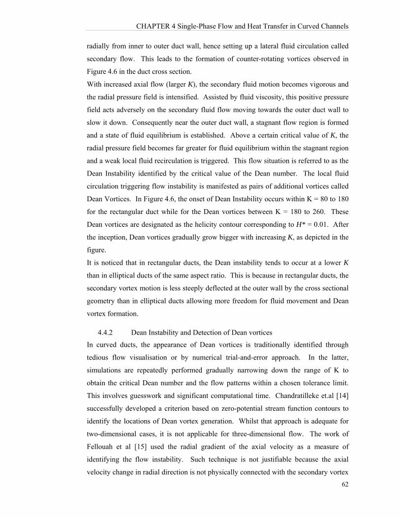
CHAPTER 4 Single-Phase Flow and Heat Transfer in Curved Channels
62
radially from inner to outer duct wall, hence setting up a lateral fluid circulation called
secondary flow. This leads to the formation of counter-rotating vortices observed in
Figure 4.6 in the duct cross section.
With increased axial flow (larger K), the secondary fluid motion becomes vigorous and
the radial pressure field is intensified. Assisted by fluid viscosity, this positive pressure
field acts adversely on the secondary fluid flow moving towards the outer duct wall to
slow it down. Consequently near the outer duct wall, a stagnant flow region is formed
and a state of fluid equilibrium is established. Above a certain critical value of K, the
radial pressure field becomes far greater for fluid equilibrium within the stagnant region
and a weak local fluid recirculation is triggered. This flow situation is referred to as the
Dean Instability identified by the critical value of the Dean number. The local fluid
circulation triggering flow instability is manifested as pairs of additional vortices called
Dean Vortices. In Figure 4.6, the onset of Dean Instability occurs within K = 80 to 180
for the rectangular duct while for the Dean vortices between K = 180 to 260. These
Dean vortices are designated as the helicity contour corresponding to H* = 0.01. After
the inception, Dean vortices gradually grow bigger with increasing K, as depicted in the
figure.
It is noticed that in rectangular ducts, the Dean instability tends to occur at a lower K
than in elliptical ducts of the same aspect ratio. This is because in rectangular ducts, the
secondary vortex motion is less steeply deflected at the outer wall by the cross sectional
geometry than in elliptical ducts allowing more freedom for fluid movement and Dean
vortex formation.
4.4.2 Dean Instability and Detection of Dean vortices
In curved ducts, the appearance of Dean vortices is traditionally identified through
tedious flow visualisation or by numerical trial-and-error approach. In the latter,
simulations are repeatedly performed gradually narrowing down the range of K to
obtain the critical Dean number and the flow patterns within a chosen tolerance limit.
This involves guesswork and significant computational time. Chandratilleke et.al [14]
successfully developed a criterion based on zero-potential stream function contours to
identify the locations of Dean vortex generation. Whilst that approach is adequate for
two-dimensional cases, it is not applicable for three-dimensional flow. The work of
Fellouah et al [15] used the radial gradient of the axial velocity as a measure of
identifying the flow instability. Such technique is not justifiable because the axial
velocity change in radial direction is not physically connected with the secondary vortex
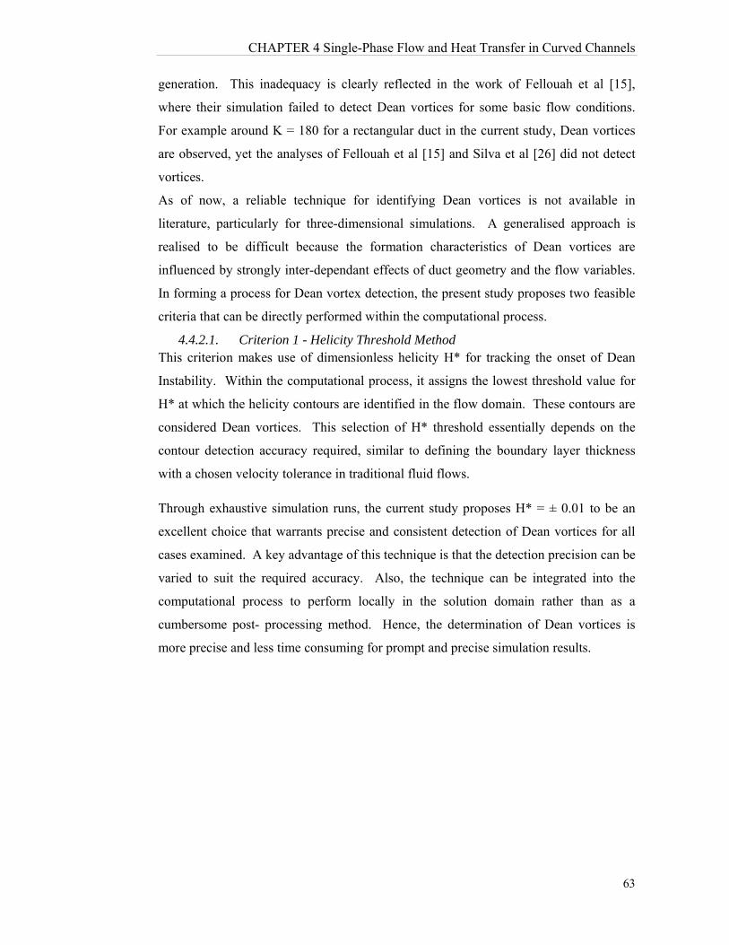
CHAPTER 4 Single-Phase Flow and Heat Transfer in Curved Channels
63
generation. This inadequacy is clearly reflected in the work of Fellouah et al [15],
where their simulation failed to detect Dean vortices for some basic flow conditions.
For example around K = 180 for a rectangular duct in the current study, Dean vortices
are observed, yet the analyses of Fellouah et al [15] and Silva et al [26] did not detect
vortices.
As of now, a reliable technique for identifying Dean vortices is not available in
literature, particularly for three-dimensional simulations. A generalised approach is
realised to be difficult because the formation characteristics of Dean vortices are
influenced by strongly inter-dependant effects of duct geometry and the flow variables.
In forming a process for Dean vortex detection, the present study proposes two feasible
criteria that can be directly performed within the computational process.
4.4.2.1. Criterion 1 - Helicity Threshold Method This criterion makes use of dimensionless helicity H* for tracking the onset of Dean
Instability. Within the computational process, it assigns the lowest threshold value for
H* at which the helicity contours are identified in the flow domain. These contours are
considered Dean vortices. This selection of H* threshold essentially depends on the
contour detection accuracy required, similar to defining the boundary layer thickness
with a chosen velocity tolerance in traditional fluid flows.
Through exhaustive simulation runs, the current study proposes H* = ± 0.01 to be an
excellent choice that warrants precise and consistent detection of Dean vortices for all
cases examined. A key advantage of this technique is that the detection precision can be
varied to suit the required accuracy. Also, the technique can be integrated into the
computational process to perform locally in the solution domain rather than as a
cumbersome post- processing method. Hence, the determination of Dean vortices is
more precise and less time consuming for prompt and precise simulation results.

Figure 4.
Figure 4.7
using H*
arrows). F
K = 95. T
increase in
detectable
reduced to
duct and K
result in a
computati
threshold
of accurac
superior t
Fellouah e
4.4.2.2This criter
wall, whic
For sever
profiles ev
CHA
K=95 Onset of In
Rectangu.7. Detection
7 shows th
= 0.01, jus
For the rect
The helicity
n K at 102.
e within K =
o obtain mo
K =234 for
a marginal
onal deman
for detectin
cy, flexibilit
to any rep
et al [15] us
2. Criterrion is base
ch is seen t
ral Dean N
valuated fro
APTER 4 Si
K
nstability at Kular duct, Ar
n of Dean vor
he helicity c
st before an
tangular du
y contours
Similarly f
= 230 to 23
ore precise
r the ellipti
benefit tow
nd. Theref
ng Dean Ins
ty or ability
orted appro
ing the axia
ion 2 - Adved on the fea
to have a st
Numbers, Fi
om Equatio
Dea
n vo
rtic
es
ingle-Phase
K=102 K = 100 r = 4 rtex formatio
contours ob
nd just afte
uct, the Dean
depicting D
for the ellip
5. By usin
K for Dean
cal duct. H
wards prec
fore, H* =
stability. P
y for vortex
oach includ
al velocity g
erse Wall Patures of the
trong affilia
igure 4.8 s
on.4.8 for a
e Flow and H
K=230Onset o
Ellon using heli
btained from
er the onse
n vortices a
Dean vortic
tical duct, t
g H* 0.0
n Instability
However, th
ision, as n
0.01 is con
Previous me
x detection,
ding that b
gradient.
Pressure Grae fluid pres
ation with t
shows typic
a rectangula
Heat Transf
0 of Instabilityliptical duct,icity threshol
m the helic
et of Dean
are initially
es are first
the appearan
1, this rang
y, as K = 1
he use of H
oted above
ncluded to
ethods neve
signifying
by Ghia an
adient Methsure gradien
the appeara
cal outer w
ar duct in F
Dea
n vo
rtic
es
fer in Curve
K=235 y at K = 234 , Ar = 4 ld method H
city thresho
vortices (in
absent in t
detected w
nce of Dean
e can be pr
00 for the
H* 0.01 w
e while incr
be a very
er provided
that this me
nd Shokhey
hod nt along the
ance of Dea
wall pressur
Figure 4.8 (
ed Channels
64
* = ± 0.01
old method
ndicated by
he flow for
with a slight
n vortices is
rogressively
rectangular
would only
reasing the
appropriate
this degree
ethod is far
y [10] and
e outer duct
an vortices.
re gradient
(a) and, for
s
4
d
y
r
t
s
y
r
y
e
e
e
r
d
t
.
t
r
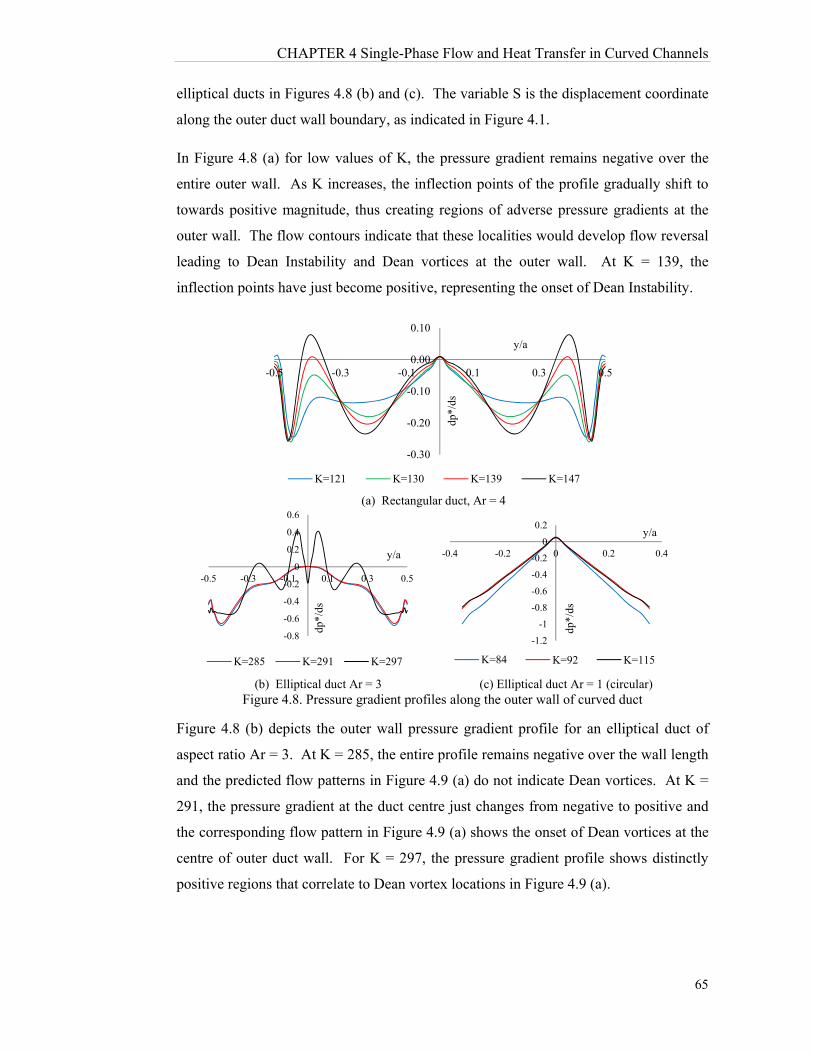
CHAPTER 4 Single-Phase Flow and Heat Transfer in Curved Channels
65
elliptical ducts in Figures 4.8 (b) and (c). The variable S is the displacement coordinate
along the outer duct wall boundary, as indicated in Figure 4.1.
In Figure 4.8 (a) for low values of K, the pressure gradient remains negative over the
entire outer wall. As K increases, the inflection points of the profile gradually shift to
towards positive magnitude, thus creating regions of adverse pressure gradients at the
outer wall. The flow contours indicate that these localities would develop flow reversal
leading to Dean Instability and Dean vortices at the outer wall. At K = 139, the
inflection points have just become positive, representing the onset of Dean Instability.
(a) Rectangular duct, Ar = 4
(b) Elliptical duct Ar = 3 (c) Elliptical duct Ar = 1 (circular) Figure 4.8. Pressure gradient profiles along the outer wall of curved duct
Figure 4.8 (b) depicts the outer wall pressure gradient profile for an elliptical duct of
aspect ratio Ar = 3. At K = 285, the entire profile remains negative over the wall length
and the predicted flow patterns in Figure 4.9 (a) do not indicate Dean vortices. At K =
291, the pressure gradient at the duct centre just changes from negative to positive and
the corresponding flow pattern in Figure 4.9 (a) shows the onset of Dean vortices at the
centre of outer duct wall. For K = 297, the pressure gradient profile shows distinctly
positive regions that correlate to Dean vortex locations in Figure 4.9 (a).
-0.30
-0.20
-0.10
0.00
0.10
-0.5 -0.3 -0.1 0.1 0.3 0.5
dp*/
ds
y/a
K=121 K=130 K=139 K=147
-0.8
-0.6
-0.4
-0.2
0
0.2
0.4
0.6
-0.5 -0.3 -0.1 0.1 0.3 0.5
dp*/
ds
y/a
K=285 K=291 K=297
-1.2
-1
-0.8
-0.6
-0.4
-0.2
0
0.2
-0.4 -0.2 0 0.2 0.4
dp*/
ds
y/a
K=84 K=92 K=115
CHAPTER 4 Single-Phase Flow and Heat Transfer in Curved Channels
66
K=285 K=291 (critical value) K=297
(a) Helicty contours for elliptical duct of aspect ratio Ar = 3
K=196 K=218 (critical value) K=229
(b) Helicty contours for elliptical duct of aspect ratio Ar = 2
K = 84 K = 92 (critical value) K = 115
(c) Helicty contours for circular duct of aspect ratio Ar = 1
Figure 4.9. Dean vortex formation in elliptical ducts of different aspect ratios (detected using H* = 0.01)
Above observations conclusively indicate that the adverse or positive pressure gradients
at the outer duct wall could be effectively used for detecting the onset and location of
Dean vortices. However, this approach has some drawback as discussed below.
Figure 4.8 (c) shows the outer wall pressure gradient for an elliptical duct of aspect ratio
Ar = 1 (circular). It does not exhibit the negative-to-positive changeover in pressure
gradient as with elliptical ducts having Ar > 1 shown in Figures 4.8 (a) and 4.8 (b).
This means the Dean vortices are not predicted according to this criterion. Based on the
helicity criterion however, Figure 4.8 (c) indeed shows the onset of Dean vortices at K
=92 in the flow. This may seem a contradiction that is clarified below.
11
11
12
12
12 13
13
13
14
15
16
17
1
34
5
67
8
8
8
9
9
10
11
10
11
11
12
12
12
13
13
1314
14
1516 171819
20
1 2
3
4
56
7
7
8
8
8
9
9
9
10
1011
11
7
8
8
9
9
10
1011
11
11
12
12
12
12
13
13
13
14
14
15
15
16
17
1819
20
2
3
45
6
6
7
7
8
8
8
8
9
9
9
11
11
12
13
13
9
9
10
10
11
11
11
12
12
12
13
13
14
1415
16
34
5
5
6
6
7
7
8
8
8
8
9
9
108
8 9
9
9
10
10
10
11
11
11
11
12
12
13 13
14
14
1515
16
23
4
5
5
6
67
7
8
8
9
9
9
10
9
10
10
10
11
11
11
11
12
12
12
13
13
14
1415
16
12 3
4
5
5
6
6
67
7
7
8
8
8
8
9
9
10
10
34
4
5
5
6
6
6
7
7
8
8
8
9
9
9
9
1010
10 10
10
11
111112 12
12
13
13
13
13
14
14
1414
15
15
15
16
16
16
17
17
17
18
1819
20
34
4
5
5
6
67
7
7
8 8
8
9
9
9
9
1010
10 10
11
11
11
11
12
12
12
13
13 13 13
14
14 14
15
15
15 15
16
16 16
17
17
18
18
19
20
3 34
4
5
56
6
6
7
7
7
8
8
8
8
9
9
9
9
10
10
10
10
10
11
11
11
11 11
12
12
12
12
12
13
13
13
13
14
14
14
14
15
15
15 15
16
16
16
17
17
17
18
18 18
19
1920 2021
Ons
et o
f D
ean
Vor
tices
Ons
et o
f D
ean
Vor
tices
Ons
et o
f D
ean
Vor
tice
s

CHAPTER 4 Single-Phase Flow and Heat Transfer in Curved Channels
67
Figure 4.9 (c) helicity contours show that, for a duct with Ar = 1, the Dean vortices do
not appear at the outer wall like in other duct shapes, but initiated in the centre of the
flow. Therefore, the outer wall pressure gradient has lesser bearing on the Dean
Instability and Dean vortex formation. As such, the pressure gradient criterion has
reduced applicability for elliptical ducts with aspect ratio near unity and tends to over
predict the critical Dean Number for instability. It would perform satisfactorily as
aspect ratio increases where it could be seen for cases with Ar>1. Overviewing both
approaches, the helicity threshold method is recognised to be precise and reliable for
detecting the Dean vortices with universal applicability for curved ducts of any shape
and aspect ratio.Dean vortices always form initially inside the flow domain close to the
outer wall (not attached to it) at the onset of this flow condition. The exact position of
these vortices depends on the duct aspect ratio and the cross sectional geometry. Figure
4.10 allows correlation of the pressure gradient and the corresponding vortex position
based on helicity while outer wall is located at left side. The figurers indicates that, at
low flow rates, the helicity approach identifies the appearance of Dean vortices while
the pressure gradient remains negative, meaning that the latter approach does not
capture this existence of vortices. Also, it is noted that Dean vortices appear not at the
outer wall but in the bulk fluid away from the wall. However, with increased flow rate,
Dean vortices will gradually migrate towards the outer wall wherein the pressure
gradient becomes adverse (or positive) and both criteria are able to capture Dean
vortices.
K=140 K=155 K=200
Figure 4.10. Comparison of two criteria for identifying the onset of Dean instability curved duct
exit plane (θ=180̊) for different flow rates, Ar = 4
-0.5
-0.4
-0.3
-0.2
-0.1
0
0.1
0.2
0.3
0.4
0.5
-0.30.2
y/a
dp*/ds
-0.5
-0.4
-0.3
-0.2
-0.1
0
0.1
0.2
0.3
0.4
0.5
-0.3
y/a
dp*/ds
-0.5
-0.4
-0.3
-0.2
-0.1
0
0.1
0.2
0.3
0.4
0.5
-0.8
y/a
dp*/ds
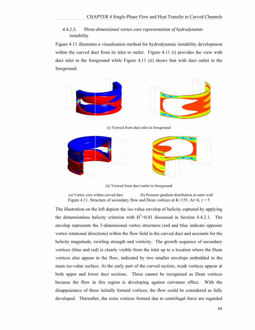
4.4.2.3ins
Figure 4.1
within the
duct inlet
foreground
(a) VFigu
The illustr
the dimen
envelop re
vortex rota
helicity m
vortices (b
vortices a
main iso-v
both uppe
because th
disappeara
developed
CHA
3. Three-stability
11 illustrate
e curved du
in the fore
d.
Vortex core wure 4.11. Stru
ration on the
nsionless he
epresents th
ational dire
magnitude, s
blue and red
also appear
value surfac
er and lowe
he flow in
ance of thes
d. Thereafte
APTER 4 Si
-dimensiona
s a visualisa
uct from its
eground wh
(i) Vie
(ii) Vie
within curved ducture of sec
e left depict
elicity crite
he 3-dimens
ctions) with
wirling stre
d) is clearly
in the flow
ce. At the e
er duct sec
n this regio
se initially
er, the extra
ingle-Phase
al vortex co
ation metho
inlet to ou
hile Figure
ewed from du
ewed from duc
duct condary flow
ts the iso-va
erion with H
sional vorte
hin the flow
ength and v
y visible fro
w, indicated
early part of
ctions. The
on is devel
formed vor
a vortices f
e Flow and H
ore represen
od for hydro
tlet. Figure
4.11 (ii) sh
ct inlet in fore
ct outlet in for
(b) Pressurew and Dean v
alue envelop
H*=0.01 dis
ex structure
w field in the
vorticity. Th
om the inlet
d by two sm
f the curved
ese cannot
loping agai
rtices, the f
formed due
Heat Transf
ntation of hy
odynamic in
e 4.11 (i) p
hows that w
eground
reground
e gradient distvortices at K=
p of helicity
scussed in
es (red and
e curved du
he growth s
t up to a loc
maller enve
d section, w
be recogni
inst curvatu
flow could b
to centrifu
fer in Curve
ydrodynami
nstability de
provides the
with duct o
tribution at ou=155, Ar=4,
y captured b
Section 4.4
blue indica
ct and acco
sequence of
cation wher
elops embed
weak vortice
ised as De
ure effect.
be consider
ugal force ar
ed Channels
68
ic
evelopment
e view with
utlet in the
uter wall = 5
by applying
4.2.1. The
ate opposite
unts for the
f secondary
re the Dean
dded in the
es appear at
an vortices
With the
red as fully
re regarded
s
8
t
h
e
g
e
e
e
y
n
e
t
s
e
y
d
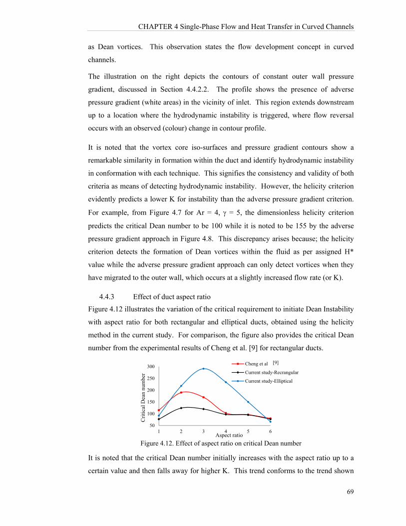
CHAPTER 4 Single-Phase Flow and Heat Transfer in Curved Channels
69
as Dean vortices. This observation states the flow development concept in curved
channels.
The illustration on the right depicts the contours of constant outer wall pressure
gradient, discussed in Section 4.4.2.2. The profile shows the presence of adverse
pressure gradient (white areas) in the vicinity of inlet. This region extends downstream
up to a location where the hydrodynamic instability is triggered, where flow reversal
occurs with an observed (colour) change in contour profile.
It is noted that the vortex core iso-surfaces and pressure gradient contours show a
remarkable similarity in formation within the duct and identify hydrodynamic instability
in conformation with each technique. This signifies the consistency and validity of both
criteria as means of detecting hydrodynamic instability. However, the helicity criterion
evidently predicts a lower K for instability than the adverse pressure gradient criterion.
For example, from Figure 4.7 for Ar = 4, = 5, the dimensionless helicity criterion
predicts the critical Dean number to be 100 while it is noted to be 155 by the adverse
pressure gradient approach in Figure 4.8. This discrepancy arises because; the helicity
criterion detects the formation of Dean vortices within the fluid as per assigned H*
value while the adverse pressure gradient approach can only detect vortices when they
have migrated to the outer wall, which occurs at a slightly increased flow rate (or K).
4.4.3 Effect of duct aspect ratio
Figure 4.12 illustrates the variation of the critical requirement to initiate Dean Instability
with aspect ratio for both rectangular and elliptical ducts, obtained using the helicity
method in the current study. For comparison, the figure also provides the critical Dean
number from the experimental results of Cheng et al. [9] for rectangular ducts.
Figure 4.12. Effect of aspect ratio on critical Dean number
It is noted that the critical Dean number initially increases with the aspect ratio up to a
certain value and then falls away for higher K. This trend conforms to the trend shown
50
100
150
200
250
300
1 2 3 4 5 6
Cri
tica
l Dea
n nu
mbe
r
Aspect ratio
Cheng et al [6]
Current study-Recrangular
Current study-Elliptical
[9]

CHAPTER 4 Single-Phase Flow and Heat Transfer in Curved Channels
70
in Figure 4.9 for elliptical ducts and the observations reported in previous experimental
and numerical work. For rectangular ducts, the current model under-predicts the critical
requirement for Dean Instability compared to the experimental results of [9]. This is
because, the helicity method identifies Dean vortices much early in the growth process,
whilst in experiments, the vortices are visually observed after they have grown to a
detectable size at a higher Dean number.
4.4.4 Thermal characteristics and Forced convection
4.4.4.1. Effects of flow rate The helicity contours and the fluid temperature fields in Figure 4.13 illustrate the effect
of outer wall heating in rectangular and elliptical ducts for two selected values of K.
The comparison of helicity contours in Figures 4.13 and 4.6 indicates the wall heating
essentially sets up a convective fluid circulation that interacts with the secondary flow
and significantly alters the flow characteristics. This fluid circulation is driven by the
buoyancy forces resulting from thermally-induced density changes.
As evident in Figure 4.13 for K=80, at low flow rates, the convective circulation
dominates the flow behaviour with less influence from secondary vortices. When the
flow rate is increased, the centrifugal action intensifies and more vigorous secondary
flow develops in the duct. Consequently, the secondary vortices overcome the thermal
buoyancy effects to become more dominant and determine the overall fluid behaviour,
as illustrated in Figure 4.13 for K=380.
Due to the confined geometry, the fluid flow within elliptical ducts is generally more
constrained and tends to have steeper fluid flow gradients than in rectangular ducts.
This geometrical effect is more pronounced at low flow rate when the flow patterns are
dominated by thermally-induced buoyancy.
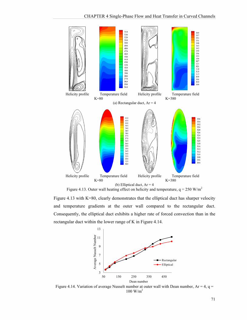
Heli
Heli
Fig
Figure 4.1
and temp
Consequen
rectangula
Figure 4.1
CHA
icity profile
icity profile
gure 4.13. Ou
13 with K=8
perature gra
ntly, the ell
ar duct with
14. Variation
APTER 4 Si
TemperaK=80
TemperaK=80
uter wall heat
80, clearly d
adients at
liptical duct
hin the lower
n of average N
3
5
7
9
11
13
50
Ave
rage
Nus
selt
Num
ber
ingle-Phase
ature field
(a) Rectangul
ature field
(b) Ellipticating effect on
demonstrate
the outer
t exhibits a
r range of K
Nusselt num100
150 25
De
e Flow and H
Helicity pr
lar duct, Ar =
Helicity pr
al duct, Ar = 4n helicity an
es that the e
wall com
higher rate
K in Figure
mber at outer wW/m2
50 350
ean number
Heat Transf
rofile TK=38
4
rofile TK=38
4 d temperatur
elliptical du
mpared to
e of forced
4.14.
wall with De
450
Rectangul
Elliptical
fer in Curve
Temperature fi0
Temperature fi0
re, q = 250 W
ct has sharp
the rectang
convection
ean number,
lar
ed Channels
71
ield
ield
W/m2
per velocity
gular duct.
than in the
Ar = 4, q =
s
y
.
e
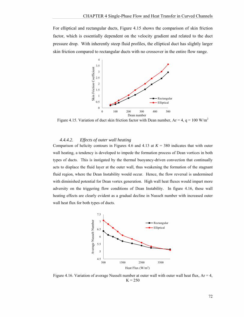
CHAPTER 4 Single-Phase Flow and Heat Transfer in Curved Channels
72
For elliptical and rectangular ducts, Figure 4.15 shows the comparison of skin friction
factor, which is essentially dependent on the velocity gradient and related to the duct
pressure drop. With inherently steep fluid profiles, the elliptical duct has slightly larger
skin friction compared to rectangular ducts with no crossover in the entire flow range.
Figure 4.15. Variation of duct skin friction factor with Dean number, Ar = 4, q = 100 W/m2
4.4.4.2. Effects of outer wall heating Comparison of helicity contours in Figures 4.6 and 4.13 at K = 380 indicates that with outer
wall heating, a tendency is developed to impede the formation process of Dean vortices in both
types of ducts. This is instigated by the thermal buoyancy-driven convection that continually
acts to displace the fluid layer at the outer wall, thus weakening the formation of the stagnant
fluid region, where the Dean Instability would occur. Hence, the flow reversal is undermined
with diminished potential for Dean vortex generation. High wall heat fluxes would impart more
adversity on the triggering flow conditions of Dean Instability. In figure 4.16, these wall
heating effects are clearly evident as a gradual decline in Nusselt number with increased outer
wall heat flux for both types of ducts.
Figure 4.16. Variation of average Nusselt number at outer wall with outer wall heat flux, Ar = 4, K = 250
0
0.5
1
1.5
2
2.5
3
3.5
4
0 100 200 300 400 500
Skin
Fri
ctio
n C
oeff
icie
nt
Dean number
Rectangular
Elliptical
4.5
5
5.5
6
6.5
7
7.5
500 1500 2500 3500
Ave
rage
Nus
selt
Num
ber
Heat Flux (W/m2)
Rectangular
Elliptical

CHAPTER 4 Single-Phase Flow and Heat Transfer in Curved Channels
73
With high wall heat fluxes, thermally induced convective circulation becomes stronger,
imparting additional resistance to the axial fluid motion. This effect is more
pronounced in elliptical ducts than in rectangular ducts. Consequently, duct skin
friction coefficient tends to be relatively higher for elliptical ducts while indicating
some increase with the wall heat flux, as evident in Figure 4.17.
Fig. 14
Figure 4.17. Variation of average duct Skin Friction with outer wall heat flux, Ar = 4, K = 250
4.4.4.3. Thermal optimisation Figure 4.18 shows the Bejan number (Be) distribution in curved duct cross sections. For both
rectangular and elliptical ducts at lower K, the flow irreversibility is practically dominated by
the entropy generation from wall heat transfer (Be 1 with a red cast) over the entire flow cross
section. As K increases, Bejan Number contours gradually acquire magnitudes less than 1
indicated by the blue cast. This signifies that in curved ducts, the secondary flow provides
favourable fluid mixing to transport the hot fluid away from the heated wall, which in turn will
improve forced convection.
K = 400 K = 1000 K = 1600
Figure 4.18. Bejan Number contours for rectangular and elliptical curved ducts, q = 100 W/m2
1
1.2
1.4
1.6
1.8
2
2.2
2.4
500 1500 2500 3500
Skin
Fri
ctio
n C
oeff
icie
nt
Wall Heat Flux (W/m2)
Rectangular
Elliptical

CHAPTER 4 Single-Phase Flow and Heat Transfer in Curved Channels
74
Magnitudes of Be 1 also signifies an increased contribution to the total irreversibility
from viscous effects, which would negate the overall flow benefits. These effects are
less pronounced in rectangular ducts than in elliptical ducts. The opposing thermal and
hydrodynamic trends identify a potentially useful technique for thermal optimisation of
fluid flow through heated curved ducts, as explained below.
Figure 4.19 illustrates the variation of the flow irreversibility components St, Sp and Sg
for rectangular and elliptical ducts with K, evaluated using Equation 4.9 and 4.10. It is
evident from the figure that, when K is increased, St steadily falls while Sp rapidly
grows. Although this falling trend is similar to both types of ducts, the thermal
irreversibility component St decays more gently in elliptical duct compared to the
rectangular duct. This means, the elliptical duct is less efficient in transporting heat
from the wall than the rectangular duct. On the other hand, the viscous irreversibility
component Sp grows more rapidly in elliptical ducts, signifying that the elliptical shape
causes higher frictional pressure loses.
(a) Rectangular duct
(b) Elliptical duct
Figure 4.19. Curved duct thermal optimisation using total entropy generation
0
0.1
0.2
0.3
0.4
0.5
0.6
0.7
0.8
0.9
1
250 750 1250
Irre
vers
ibil
ty c
ompo
nent
s S
t, S
p,Sg
Dean Number
StSpSg
0
0.2
0.4
0.6
0.8
1
250 750 1250
Irre
vers
ibil
ty c
ompo
nent
s S
t, S
p,
Sg
Dean Number
StSpSg
CHAPTER 4 Single-Phase Flow and Heat Transfer in Curved Channels
75
The overall irreversibility Sg, which is the sum of St and Sp, is initially dominated by
the thermal irreversibility component and steadily falls with K for both duct shapes.
However, the falling gradient is steeper for the rectangular duct, which implies more
effectiveness heat transfer in the fluid domain with lesser adversity from viscous effects.
At a certain value of K, Sg shows a minimum magnitude. This point of inflection is
identified as practically the best possible “trade-off” between the highest achievable
thermal benefits with the least viscous penalty for curved duct flows. It is noted that the
magnitude of the lowest overall irreversibility is higher for elliptical ducts than for
rectangular ducts, indicating rectangular ducts would thermally better perform.
4.5. Summary
This chapter provides a broad overview of the reported findings from the published
numerical and experimental studies on fluid flow in curved duct geometries. The
discussion then focusses on the latest contributions to new knowledge in this field by
extensive research programmers of the authors where new analytical techniques and
methodologies have been discovered, warranting a clearer fundamental understanding
on fluid and thermal behaviour in curved ducts.
Improving accuracy over previous methods, the current study formulates a new three-
dimensional simulation methodology based on helicity that realistically represent the
secondary vortex structures in curved ducts of any shape. The model accurately
identifies and predicts unique features of secondary flow and the associated forced
convection in both rectangular and elliptical curved ducts. Conforming to the limited
data in literature, the predicted results examine the effects of fluid flow rate, duct aspect
ratio and heat flux over a wide practical range. The duct geometry and aspect ratio are
found to have critical influence on the secondary flow characteristics, indicating a
profound effect on Dean vortex formation, Dean Instability and forced convection.
Elliptical ducts show marginally inferior thermal performance compared to rectangular
ducts under identical flow conditions.
Overcoming a current analytical limitation, this part of study appraises two novel
methods for detecting the onset of Dean Instability in curved ducts, confirming their
technical feasibility. One such approach uses a defined helicity threshold while the
other makes use of features of the outer wall pressure gradient. Both methods offer the
option of being able to be integrated into and performed within a computational scheme,
CHAPTER 4 Single-Phase Flow and Heat Transfer in Curved Channels
76
for fast, reliable and accurate detection of Dean vortex formation. However, the helicity
threshold method is realized to be more universally applied to all duct shapes and aspect
ratios. The pressure gradient approach shows limited functionality for it over-predicts
the critical Dean Number in curved ducts of aspect ratio near unity.
The study also develops a useful thermal optimization technique for heated curved duct
based on the Second Law irreversibilities. It identifies the elliptical ducts to have less
favourable overall thermal and hydrodynamics characteristics than rectangular ducts.

CHAPTER 5 Immiscible Two-Phase Fluid Flow in Curved Channels
77
CHAPTER 5
CHAPTER 5 Immiscible Two-Phase Fluid Flow in Curved Channels
5.1. Scope of Chapter
This chapter investigates the behaviour of two non-mixing fluids flowing in a heated
curved channel. In simulating this immiscible fluid flow, a multi-phase model based on
VOF approach is developed for steady, turbulent, incompressible fluid flow through
curved channel. The analysis examines the influence of centrifugal forces arising from
channel curvature on the phase distribution and flow patterns, and their impact on the
thermal characteristics. Unique flow features are identified through the interactions
between the fluid phases and vortex structures of the immiscible flow in curved
channels. The convective heat transfer in curved channel is appraised in relation to the
behaviour of fluid components and curved channel flow parameters. Finally, the
chapter presents a Second Law irreversibility analysis whereby a thermal optimisation
technique is developed for immiscible fluid flow through heated curved channels.
5.2. Introduction
Non-mixing multi-component fluid flows often occur in many industrial applications.
Some such examples are the transportation of crude oil mixed with water in oil and gas
industry, the chemical fluid flow within reactors in pharmaceutical production processes
[66] and, the flow of lubricant and refrigerant mixtures in refrigeration systems [67, 68].
The flow behaviour of two-phase immiscible fluids is uniquely different to both single
phase fluids and two-phase flow boiling. Such fluids exhibit unusual flow dynamics
because, immiscible fluid components may have differential flow (slip) velocities and
do not undergo mass exchanges albeit heat transfer may occur over phase boundaries.
Thus, the flow behaviour of non-mixing fluids is critically dominated by the relative
magnitudes of fluid component properties, in particular the density and viscosity. In
CHAPTER 5 Immiscible Two-Phase Fluid Flow in Curved Channels
78
curved channels, the centrifugal forces arising from channel curvature affect more on
the heavier of the fluid components. These combined interactions determine the
distribution, deformation and interface area of phases, and the flow regimes in
immiscible fluid flow. Resulting flow patterns, phase separation, pressure drop and heat
transfer characteristics are uniquely different to other types of fluid flows.
Consequently, for the development of industrial equipment involving non-mixing fluids,
new design methodologies are necessary with a clearer fundamental understanding of
immiscible flow behaviour.
Much research has been conducted on immiscible fluid mixtures flowing in straight
channels. These typically examine the phase instability arising from the viscosity
differences and report substantial influence on fluid and thermal characteristics [69,70].
To the contrary, immiscible fluid flow in curved channels has not much been
investigated and many fundamental aspects still remain unexplored in spite of
significant applications in process industries.
Multi-phase fluid flow systems are inherently chaotic and potentially unstable due to
non-homogeneous fluid properties that create imbalances in flow dynamics. In curved
channels, additional complexities appear because of the centrifugal action that induce
secondary flow effects and create the possibility of Dean Instability in the fluid.
In single phase fluid flow through curved passages, the presence of secondary flow and
Dean vortices is fundamentally linked to the interaction between fluid inertia and
viscous forces. With multi-component fluid flows in curved channels, the momentum
transfer across phase boundaries also play a role on secondary vortex formation, in
addition to the inertia and viscous effects. This is because of the fluid phases have
velocity differentials called drift velocity. Process designs ignoring these curvature
effects would lead to system inefficiencies and failures such as pipe wall erosion and
corrosion and, tube burn out due to non-uniform wall heat transfer.
In analysing immiscible fluid flow, two key transport mechanisms need to be
considered. They are the heat and momentum transfer across the interfacial phase
boundaries and the heat convection within each fluid phase [71]. Accounting for these
and the curvature-induced centrifugal effects, a numerical model is developed in this
chapter to investigate the flow of two non-mixing fluid through heated curved channels.
The simulation examines the secondary flow circulation within each fluid phase and the
CHAPTER 5 Immiscible Two-Phase Fluid Flow in Curved Channels
79
separation of phases that arise from the centrifugal action and the differential phase
velocities and fluid properties. The analysis also evaluates the impact on curved
channel heat transfer from the phase distribution and the secondary flow behaviour in
immiscible fluid flow. In examining this flow condition, the following geometry is
considered.
5.3. Geometrical Configuration and Boundary Condition
As shown in Figure 5.1, the immiscible flow simulation is performed on a semi-circular
(180o) curved duct of fixed radius of curvature, which is very similar to the geometrical
arrangement used in single-phase analysis. The coordinate system and the dimensions
used in the geometry are also given in the figure. The analysis examines the flow
within square and circular ducts. For both duct types, a 10 mm width is chosen to
permit the hydraulic diameter to be the same between them.
The analysis uses a mixture of water (heavier) and kerosene (lighter) as the immiscible
working fluid, which is fed together in to the curved channel through a straight inlet
passage. The length of this passage is adjusted depending on the flow rate to ensure
fully-developed conditions at the curved channel entry. The flow rates of these fluid
phases are independently varied. The flow within the straight section is separately
analysed to obtain the fully-developed velocity component profiles, turbulence
characteristics and distribution of volume fraction, that are used as input conditions for
curved section. This approach significantly reduces the computational demand in
analysing curved channel section for all tested flow cases.
At curved channel exit, a short passage is added to provide smooth fluid out flow. This
is critically important for multi-phase flow analysis to prevent any “outlet backflow”
and/or numerical disruption issues during computations. At this flow exit, pressure
outlet boundary condition is applied in contrast to the outlet flow boundary condition
used for single-phase flow simulation. For flow cases with wall heating, a constant heat
flux within the range of 0 to 5000 W/m2.K is applied over the entire circumference of
the curved passage.
The curved channel geometry is orientated to provide symmetrical influence from
gravity on the flow through curved channel. With this orientation, the gravitational
forces compel the heavier fluid phase (water) to move along the inner channel wall
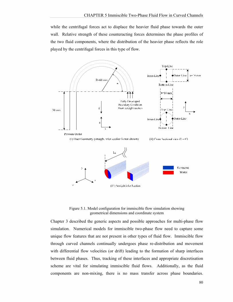
CHAPTER 5 Immiscible Two-Phase Fluid Flow in Curved Channels
80
while the centrifugal forces act to displace the heavier fluid phase towards the outer
wall. Relative strength of these counteracting forces determines the phase profiles of
the two fluid components, where the distribution of the heavier phase reflects the role
played by the centrifugal forces in this type of flow.
Figure 5.1. Model configuration for immiscible flow simulation showing geometrical dimensions and coordinate system
Chapter 3 described the generic aspects and possible approaches for multi-phase flow
simulation. Numerical models for immiscible two-phase flow need to capture some
unique flow features that are not present in other types of fluid flow. Immiscible flow
through curved channels continually undergoes phase re-distribution and movement
with differential flow velocities (or drift) leading to the formation of sharp interfaces
between fluid phases. Thus, tracking of these interfaces and appropriate discretisation
scheme are vital for simulating immiscible fluid flows. Additionally, as the fluid
components are non-mixing, there is no mass transfer across phase boundaries.

CHAPTER 5 Immiscible Two-Phase Fluid Flow in Curved Channels
81
Accordingly among the models discussed in Chapter 3, the Volume of Fraction (VOF)
approach is identified as the most suitable to handle these special requirements of
immiscible flow modelling.
Unlike Eulerian model, the VOF model solves a single set of conservation equations
incorporating equivalent density for the whole domain. This approach is adequate for
accurate prediction of phase distribution, interfacial movement and velocity fields in
immiscible flow [63, 64], drastically saving the computational effort.
The VOF approach is further enhanced by using the Level-Set method [72] that
improves the precision of phase boundary tracking. In this, the interface between two
phases is captured and tracked by the level-set function defined in terms of the sign
distance from the interface. The interface is then implicitly represented by the level set
of 0)( x and implicitly moved by the advection of )(x , which is split into two
steps. The first step of )(x is advected using a standard numerical method. Then the
second step is performed to preserve smooth profile for )(x and the transition layer
thickness. Both of these steps are executed using conservative second order
approximations for conserving )(x .
5.4. Governing Equations
As described above, a VOF model coupled with Level-Set function is used for precise
interface modelling of immiscible two-phase flow. With a specific discretisation
scheme for volume of fraction the model robustness is improved.
Level Set function, is defined by,
erface
erface
d
d
x
int
int
0)(
2
1
Phasex
x
Phasex
5.1
where, represents interface area and erfacedint is cell distance from interface
For calculating surface tension, the interface normal and curvature are obtained
according to the sign function as,

CHAPTER 5 Immiscible Two-Phase Fluid Flow in Curved Channels
82
0
n
0
.
5.2 (a)
5.2 (b)
Conservation of Level Set function is given by,
0).( u
5.3
Accounting for phase effects with the equivalent bulk density, the continuity equation is
given by,
0).( um
5.4
Taking subscript “k” to denote each phase, bulk values for a cell are described by,
n
kkkm
1
n
kkkm
1
5.5 (a)
5.5 (b)
The momentum equations for the VOF model coupled with Level-Set are derived as,
cmT
mm Fguupuu
)()()(. 22
and
0
3
)5.1/cos(1
)( gs
gs
gs
gs
5.1
5.1
where gs is grid spacing size.
5.6 (a)
5.6 (b)
Energy conservation is also a treated as a single equation for the whole domain with
bulk properties and is written as,
Tfmmmm TkTcu .)(. 2
5.7
Compared to the version of 1983, Wilcox ( k ) turbulence model, which is a modified
version of 2006, is reported to be much suited for representing turbulence similar to that
associated with secondary flow encountered in immiscible flows. For this, the key
parameters k (turbulence kinetic energy) and (specific dissipation rate) are obtained
from the most accurate version of closure [60] in tensor notation as:
CHAPTER 5 Immiscible Two-Phase Fluid Flow in Curved Channels
83
Kinematic Eddy viscosity:
~
kT ,
*lim
2,max~
ijij SS
C , 8
7lim C 5.8
Turbulence Kinetic energy:
])[( **
jjj
iij
jj x
kk
xk
x
u
x
ku
5.9
Specific dissipation rate:
])[(2
jjjj
d
j
iij
jj x
k
xxx
k
x
u
kxu
5.10
Closure coefficients and auxiliary relations:
25
13 , fo ,
10
9* , 2
1 ,
5
3* , 8
1d 5.11
0708.0o ,
1001
851
f , 3* )(
kijkij S
5.12
where
)(2
1
i
j
j
iij x
u
x
u
, )(2
1
i
j
j
iij x
u
x
uS
, 5.13
In simulation models, near-wall treatment for wall-bounded flows is a good measure of
models capabilities and precision. In -based models viscous sub-layer is solved and
matched with defect layer in contrast to classic wall function treatments. For such
cases, y needs to be small enough to stay within the sub-layer for the validity of
turbulence model at the wall. To comply with this, it is required to have high mesh
density, which becomes a model limitation for large domains, for example the two-
phase flow boiling case discussed in Chapter 6. Taking y to be the direction normal to
surface, current closure would be rewritten for the sub-layer as,
2)( uy
uT
,
~k
T ,
*lim
/,max~
yu
C
0)( *
2
*
ky
U
yd
dkk
yd
dT
0)( 20
2
yy
k
y
U
kyd
dk
yd
d dT
5.14 (a)
5.14 (b)
5.14 (c)
CHAPTER 5 Immiscible Two-Phase Fluid Flow in Curved Channels
84
For matching to defect-layer solution (i.e. asymptotic to log-layer solution), the
following limits should be satisfied:
*
2
u
k and yk
u
* as y 5.15
Using Equation 4.7 that was introduced in Chapter 4, the non-dimensional Helicity
function is now defined for each phase separately, based on applicable reference values.
Dimensionless Helicty function for phase “p” is formulated as,
PinrefhpP U
DHH
2
* 1..
5.16
This configuration facilitates the evaluation of Helicity function for each phase
according to its material properties and reference values while permitting clear
identification of vortex structure.
Fluid pressure is non-dimensionalised as,
)UU(2
1p
p2
qinqq2
pinpp
*
5.17
In this immiscible flow analysis, the pressure gradient is examined for both phases at
the inner and outer channel walls. For this, the pressure gradient is defined in
“secondary flow-wise” direction since the secondary flow would occur in opposite
directions at inner and outer channel walls. The relevant pressure gradient expressions
are identical to those for single phase flow, given in Chapter 4 by Equation 4.8.
For the Second Law analysis and thermal optimisation, the irreversibility expressions
for immiscible multi-phase turbulent flow are developed by modifying Equation 4.9 in
Chapter 4 as,
2222
)()()()1(z
T
y
T
x
T
T
k
k
kS m
m
tT
T
.k.09.0
)x
w
z
u()
z
v
y
w()
x
v
y
u(])
z
w()
y
v()
x
u[(2
TS
m
222222mP
5.18 (a)
5.18 (b)
CHAPTER 5 Immiscible Two-Phase Fluid Flow in Curved Channels
85
In these ST and SP expressions, additional irreversibility terms appear due to turbulence
structures in comparison to the laminar version given by Equation 4.9 in Chapter 4.
Volumetric averaging, total entropy and Bejan number are defined similar to single
phase model as given by Equation 4.10 and 4.11 in Chapter 4.
5.5. Grid sensitivity analysis and Mesh selection
In relation to single and two-phase flow modelling, the Chapters 3 and 4 presented a
brief discussion on generic details of grid generation, restrictions and requirements. For
ensuring the reliability of computational fluid dynamics results, a grid sensitivity
analysis is a foremost requirement by which the predicted solutions are shown to be
independent on the grid size beyond a certain threshold. In this, different grid
configurations/topologies could be attempted and/or grid size can be gradually refined
until results show no significant change.
For simulations involving turbulence closures, in addition to establishing the grid
independence, a chosen grid needs to satisfy specific turbulence modelling requirement
in terms of y near the solid wall boundaries to achieve smoother laminar to turbulent
transition. For the immiscible flow discussed in this chapter, it is required to ensure y
remains below a value of 5 throughout the solution domain [60, 63].
In the immiscible model developed in this Chapter, the analysis is carried out with a
fully hexagonal grid for both rectangular and circular channels. However, a five-zone
topology is used only for the (elliptical) circular cross section in accounting for sharp
gradients, as mentioned in Section 4.33 in Chapter 4.
Figure 5.2 presents the approach adopted to perform the grid sensitivity test and to
obtain the optimum mesh size for the immiscible flow analysis discussed in this chapter.
The primary phase volume fraction is chosen for examining the grid dependency
because this scalar parameter is readily affected by other convective terms. The volume
fraction profiles for the primary phase are evaluated at the vertical and horizontal centre
planes at the exit of rectangular and circular curved channels and are presented as four
sub-figures in Figure 5.2. Meshes 1 to 4 are the finest of the grids tested, representing
uniform grid spacing of 1.0 mm, 0.5 mm, 0.25 mm and 0.1 mm, respectively.
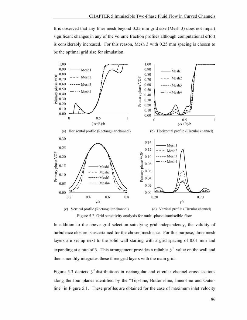
CHAPTER 5 Immiscible Two-Phase Fluid Flow in Curved Channels
86
It is observed that any finer mesh beyond 0.25 mm grid size (Mesh 3) does not impart
significant changes in any of the volume fraction profiles although computational effort
is considerably increased. For this reason, Mesh 3 with 0.25 mm spacing is chosen to
be the optimal grid size for simulation.
(a) Horizontal profile (Rectangular channel) (b) Horizontal profile (Circular channel)
(c) Vertical profile (Rectangular channel) (d) Vertical profile (Circular channel)
Figure 5.2. Grid sensitivity analysis for multi-phase immiscible flow
In addition to the above grid selection satisfying grid independency, the validity of
turbulence closure is ascertained for the chosen mesh size. For this purpose, three mesh
layers are set up next to the solid wall starting with a grid spacing of 0.01 mm and
expanding at a rate of 3. This arrangement provides a reliable y value on the wall and
then smoothly integrates these three grid layers with the main grid.
Figure 5.3 depicts y distributions in rectangular and circular channel cross sections
along the four planes identified by the “Top-line, Bottom-line, Inner-line and Outer-
line” in Figure 5.1. These profiles are obtained for the case of maximum inlet velocity
0.000.100.200.300.400.500.600.700.800.901.00
0 0.5 1
Pri
mar
y ph
ase
VO
F
(-x+R)/b
Mesh1
Mesh2
Mesh3
Mesh4
0.000.100.200.300.400.500.600.700.800.901.00
0 0.5 1
Pri
mar
y ph
ase
VO
F
(-x+R)/b
Mesh1
Mesh2
Mesh3
Mesh4
0.00
0.05
0.10
0.15
0.20
0.25
0.30
0.2 0.4 0.6 0.8
Pri
mar
y ph
ase
VO
F
y/a
Mesh1
Mesh2
Mesh3
Mesh4
0.00
0.02
0.04
0.06
0.08
0.10
0.12
0.14
0.20 0.70
Pri
mar
y ph
ase
VO
F
y/a
Mesh1
Mesh2
Mesh3
Mesh4
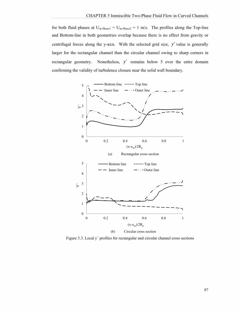
CHAPTER 5 Immiscible Two-Phase Fluid Flow in Curved Channels
87
for both fluid phases at Uin-Phase1 = Uin-Phase2 = 1 m/s. The profiles along the Top-line
and Bottom-line in both geometries overlap because there is no effect from gravity or
centrifugal forces along the y-axis. With the selected grid size, y value is generally
larger for the rectangular channel than the circular channel owing to sharp corners in
rectangular geometry. Nonetheless, y remains below 5 over the entre domain
confirming the validity of turbulence closure near the solid wall boundary.
(a) Rectangular cross section
(b) Circular cross section
Figure 5.3. Local y+ profiles for rectangular and circular channel cross sections
0
1
2
3
4
5
0 0.2 0.4 0.6 0.8 1
Y+
(x-xin)/2Rp
Bottom line Top line
Inner line Outer line
0
1
2
3
4
5
0 0.2 0.4 0.6 0.8 1
Y+
(x-xin)/2Rp
Bottom line Top line
Inner line Outer line
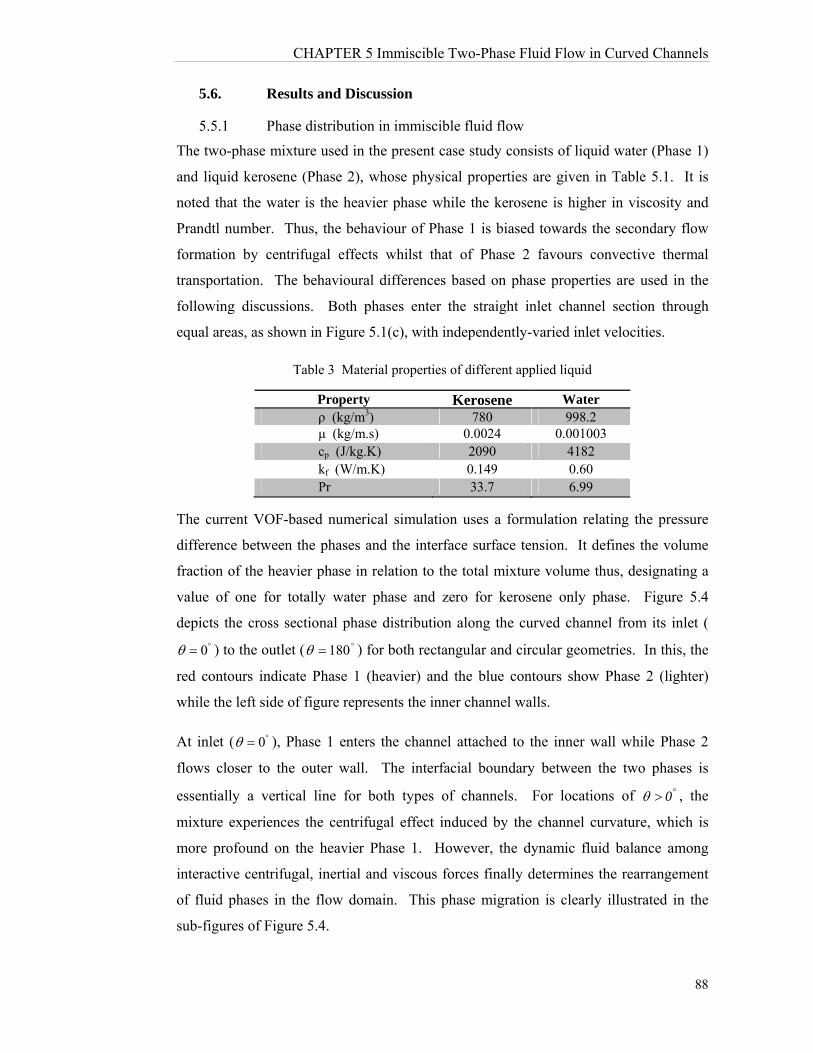
CHAPTER 5 Immiscible Two-Phase Fluid Flow in Curved Channels
88
5.6. Results and Discussion
5.5.1 Phase distribution in immiscible fluid flow
The two-phase mixture used in the present case study consists of liquid water (Phase 1)
and liquid kerosene (Phase 2), whose physical properties are given in Table 5.1. It is
noted that the water is the heavier phase while the kerosene is higher in viscosity and
Prandtl number. Thus, the behaviour of Phase 1 is biased towards the secondary flow
formation by centrifugal effects whilst that of Phase 2 favours convective thermal
transportation. The behavioural differences based on phase properties are used in the
following discussions. Both phases enter the straight inlet channel section through
equal areas, as shown in Figure 5.1(c), with independently-varied inlet velocities.
Table 3 Material properties of different applied liquid
Property Kerosene Water ρ (kg/m3) 780 998.2 μ (kg/m.s) 0.0024 0.001003 cp (J/kg.K) 2090 4182 kf (W/m.K) 0.149 0.60 Pr 33.7 6.99
The current VOF-based numerical simulation uses a formulation relating the pressure
difference between the phases and the interface surface tension. It defines the volume
fraction of the heavier phase in relation to the total mixture volume thus, designating a
value of one for totally water phase and zero for kerosene only phase. Figure 5.4
depicts the cross sectional phase distribution along the curved channel from its inlet (
0 ) to the outlet ( 180 ) for both rectangular and circular geometries. In this, the
red contours indicate Phase 1 (heavier) and the blue contours show Phase 2 (lighter)
while the left side of figure represents the inner channel walls.
At inlet ( 0 ), Phase 1 enters the channel attached to the inner wall while Phase 2
flows closer to the outer wall. The interfacial boundary between the two phases is
essentially a vertical line for both types of channels. For locations of 0 , the
mixture experiences the centrifugal effect induced by the channel curvature, which is
more profound on the heavier Phase 1. However, the dynamic fluid balance among
interactive centrifugal, inertial and viscous forces finally determines the rearrangement
of fluid phases in the flow domain. This phase migration is clearly illustrated in the
sub-figures of Figure 5.4.
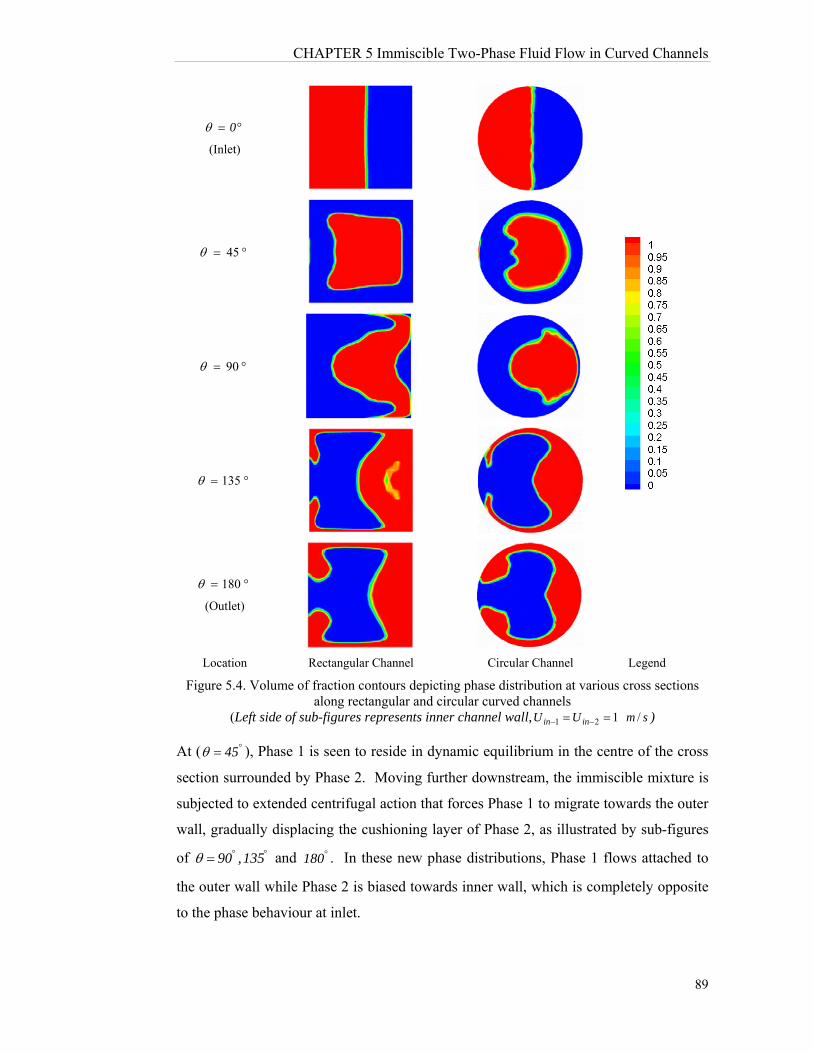
CHAPTER 5 Immiscible Two-Phase Fluid Flow in Curved Channels
89
0
(Inlet)
45
90
135
180
(Outlet)
Location Rectangular Channel Circular Channel Legend
Figure 5.4. Volume of fraction contours depicting phase distribution at various cross sections along rectangular and circular curved channels
(Left side of sub-figures represents inner channel wall, smUU inin /121 )
At ( 45 ), Phase 1 is seen to reside in dynamic equilibrium in the centre of the cross
section surrounded by Phase 2. Moving further downstream, the immiscible mixture is
subjected to extended centrifugal action that forces Phase 1 to migrate towards the outer
wall, gradually displacing the cushioning layer of Phase 2, as illustrated by sub-figures
of 135,90 and 180 . In these new phase distributions, Phase 1 flows attached to
the outer wall while Phase 2 is biased towards inner wall, which is completely opposite
to the phase behaviour at inlet.
CHAPTER 5 Immiscible Two-Phase Fluid Flow in Curved Channels
90
5.5.2 Immiscible fluid flow patterns and secondary flow vortices
Compared to other types of fluid flows, immiscible two-phase flow in curved channels
tends to have unique secondary flow behaviour because these flow characteristics are
determined by the coupled action of curvature-induced centrifugal effects and
momentum transfer between phases. These are further compounded by the density and
viscosity differences between phases that alter the relative strength of inertial, viscous
and centrifugal forces in determining the fluid flow behaviour. Consequently, each
phase essentially behaves as a separate secondary flow cell within which stagnation
regions are developed with the potential for vortex formation and hydrodynamic
instability. However due to the momentum coupling between phases, secondary flow
circulations within the phases are interlinked, giving rise to more complex flow patterns
compared to single phase fluid flow in curved channels.
The flow patterns in immiscible flow are examined by using the dimensionless helicity
function, as defined by Equation 5.16, separately for each phase. Figure 5.5 depicts the
helicity distribution for each phase along the curved channel from inlet
( 0 ) to the outlet ( 180 ) for both rectangular and circular geometries. In this,
the red and blue contours are for Phase 1 and Phase 2, respectively while the solid lines
and dashed line respectively indicate the clock-wise and counter clock-wise rotations of
fluid circulation. The left side of sub-figures in Figure 5.5 represent inner channel wall.
As evident, these secondary flow patterns are far more complex and uniquely different
to those in single phase fluid flow in curved channels.
At inlet ( 0 ), Figure 5.5 shows the initial stage of secondary vortex formation
within individual phase boundaries. At this stage, Phase 1 flows closer to the inner wall
and the fluid circulations in each phase occur in the same corresponding direction at the
top and bottom half of channel cross section. When the fluid moves downstream (
0 ), the extended centrifugal action intensifies the secondary flow circulation and
displaces Phase 2 circulation towards the inner wall, as shown by the patterns at
90 . Such pockets of highly localised secondary vortices do rotate in opposite
directions indicating the transfer of fluid momentum between adjacent vortex cells
embedded within the same phase or across phase boundaries. By the channel exit (
180 ), the momentum transfer of Phase 1 circulations become so strong to confine
Phase 2 circulation practically to the centre of channel.

CHAPTER 5 Immiscible Two-Phase Fluid Flow in Curved Channels
91
0
90
180
Location Rectangular Channel Circular Channel
Figure 5.5. Dimensionless helicity contours for immiscible flow domain (Left side of sub-figures represents inner channel wall, smUU inin /121 )
As observed above, the interactive mechanism of the secondary flow developed by
centrifugal action and the momentum transfer across phase boundaries uniquely
determine the immiscible two-phase flow behaviour in curved channels. For the case
depicted in Figure 5.5, each phase enters with an equal inlet velocity of 1 m/s, thus the
momentum transfer is not biased towards any particular phase, apart from the possible
impact of their fluid property differences. Varied phase velocity differences accentuate
the influence on secondary flow behaviour from the momentum flow across phases.
Figure 5.6 shows the effects of phase velocity ratio on secondary flow structures.
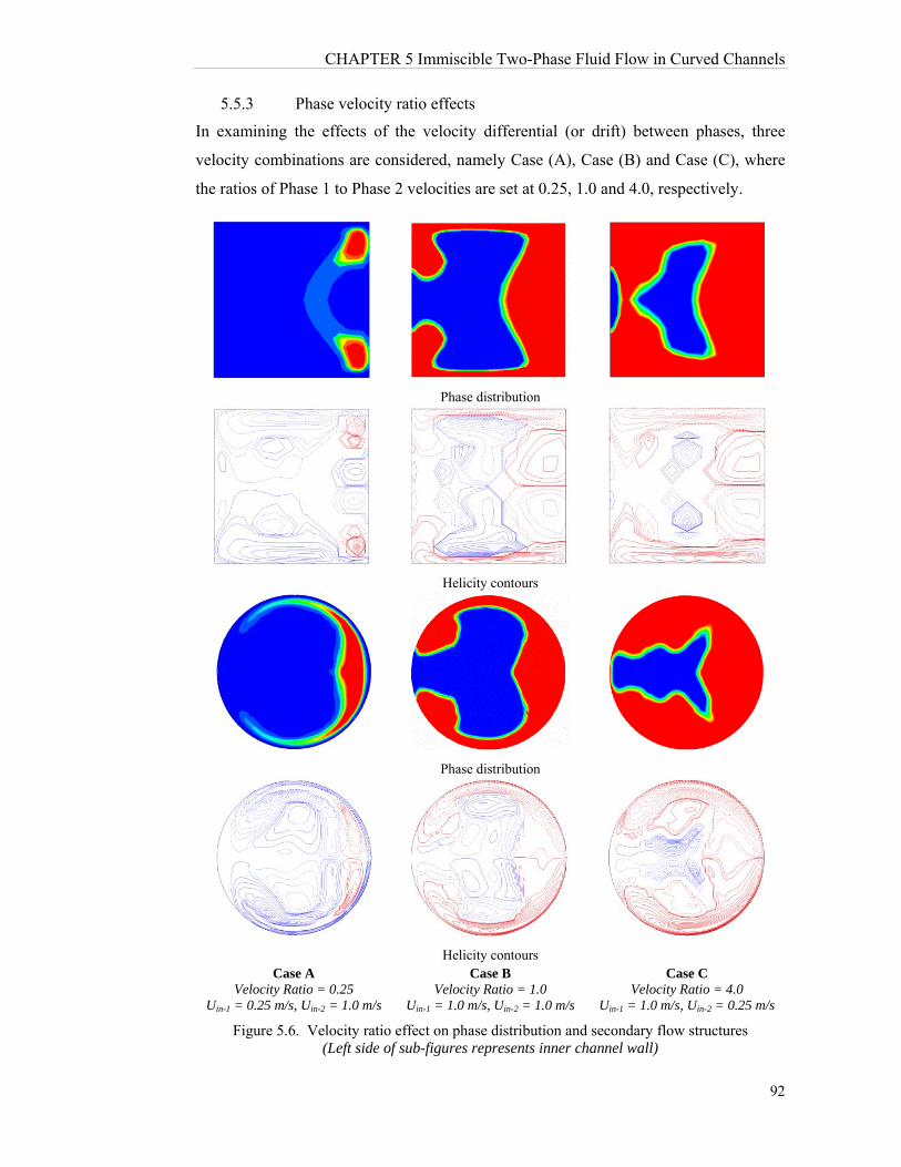
CHAPTER 5 Immiscible Two-Phase Fluid Flow in Curved Channels
92
5.5.3 Phase velocity ratio effects
In examining the effects of the velocity differential (or drift) between phases, three
velocity combinations are considered, namely Case (A), Case (B) and Case (C), where
the ratios of Phase 1 to Phase 2 velocities are set at 0.25, 1.0 and 4.0, respectively.
Phase distribution
Helicity contours
Phase distribution
Helicity contours
Case A
Velocity Ratio = 0.25 Uin-1 = 0.25 m/s, Uin-2 = 1.0 m/s
Case BVelocity Ratio = 1.0
Uin-1 = 1.0 m/s, Uin-2 = 1.0 m/s
Case C
Velocity Ratio = 4.0 Uin-1 = 1.0 m/s, Uin-2 = 0.25 m/s
Figure 5.6. Velocity ratio effect on phase distribution and secondary flow structures (Left side of sub-figures represents inner channel wall)
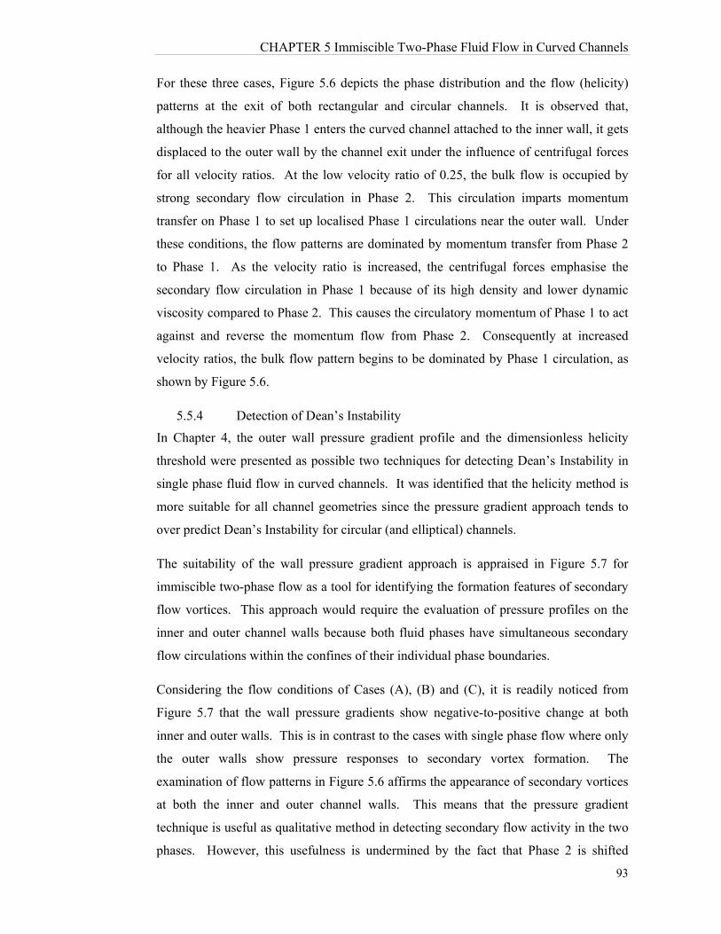
CHAPTER 5 Immiscible Two-Phase Fluid Flow in Curved Channels
93
For these three cases, Figure 5.6 depicts the phase distribution and the flow (helicity)
patterns at the exit of both rectangular and circular channels. It is observed that,
although the heavier Phase 1 enters the curved channel attached to the inner wall, it gets
displaced to the outer wall by the channel exit under the influence of centrifugal forces
for all velocity ratios. At the low velocity ratio of 0.25, the bulk flow is occupied by
strong secondary flow circulation in Phase 2. This circulation imparts momentum
transfer on Phase 1 to set up localised Phase 1 circulations near the outer wall. Under
these conditions, the flow patterns are dominated by momentum transfer from Phase 2
to Phase 1. As the velocity ratio is increased, the centrifugal forces emphasise the
secondary flow circulation in Phase 1 because of its high density and lower dynamic
viscosity compared to Phase 2. This causes the circulatory momentum of Phase 1 to act
against and reverse the momentum flow from Phase 2. Consequently at increased
velocity ratios, the bulk flow pattern begins to be dominated by Phase 1 circulation, as
shown by Figure 5.6.
5.5.4 Detection of Dean’s Instability
In Chapter 4, the outer wall pressure gradient profile and the dimensionless helicity
threshold were presented as possible two techniques for detecting Dean’s Instability in
single phase fluid flow in curved channels. It was identified that the helicity method is
more suitable for all channel geometries since the pressure gradient approach tends to
over predict Dean’s Instability for circular (and elliptical) channels.
The suitability of the wall pressure gradient approach is appraised in Figure 5.7 for
immiscible two-phase flow as a tool for identifying the formation features of secondary
flow vortices. This approach would require the evaluation of pressure profiles on the
inner and outer channel walls because both fluid phases have simultaneous secondary
flow circulations within the confines of their individual phase boundaries.
Considering the flow conditions of Cases (A), (B) and (C), it is readily noticed from
Figure 5.7 that the wall pressure gradients show negative-to-positive change at both
inner and outer walls. This is in contrast to the cases with single phase flow where only
the outer walls show pressure responses to secondary vortex formation. The
examination of flow patterns in Figure 5.6 affirms the appearance of secondary vortices
at both the inner and outer channel walls. This means that the pressure gradient
technique is useful as qualitative method in detecting secondary flow activity in the two
phases. However, this usefulness is undermined by the fact that Phase 2 is shifted
CHAPTER 5 Immiscible Two-Phase Fluid Flow in Curved Channels
94
towards the channel centre by the influence Phase 1 momentum transfer at high velocity
ratios, as depicted in Figure 5.6. As such, although the pressure gradient profile is
useful for some qualitative assessment of Dean’s Instability, it is uncertain and remains
less effective as a criterion for vortex detection in immiscible flow and, the helicity
threshold technique is considered more appropriate.
(a) Profile at inner wall (b) Profile at outer wall Figure 5.7. Wall pressure gradient at exit of rectangular channel for Cases (A) (B) (C)
From Figure 5.7, it is further observed that, sharper and larger gradients are generally
present at the outer walls, which are accentuated with increased velocity ratio. This
indicates a higher intensity of flow instability in Phase 1 compared to Phase 2, which is
clearly supported by the helicity profiles in Figure 5.6 showing a stronger presence of
vortices in Phase 1 and subdued circulation in Phase 2.
5.5.5 Behaviour of phase interfacial area
The interfacial area between fluid phases is a crucial parameter for immiscible fluid
components reacting with each other, such as in chemical processing where maximised
interfacial contact improves production efficiency. Figure 5.8 shows the ratio of
interfacial phase area for immiscible flow through curved channel (IACurved) to that in
straight channels (IAStraight) with respect to the inlet velocity ratio.
-20
-15
-10
-5
0
5
-0.5 -0.3 -0.1
dp*/
ds
y/a
Case-A
Case-B
Case-C
-50
-30
-10
10
30
50
70
90
-0.5 -0.3 -0.1
dp*\
ds
y/a
Case-A
Case-B
Case-C
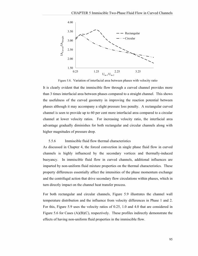
CHAPTER 5 Immiscible Two-Phase Fluid Flow in Curved Channels
95
Figure 5.8. Variation of interfacial area between phases with velocity ratio
It is clearly evident that the immiscible flow through a curved channel provides more
than 3 times interfacial area between phases compared to a straight channel. This shows
the usefulness of the curved geometry in improving the reaction potential between
phases although it may accompany a slight pressure loss penalty. A rectangular curved
channel is seen to provide up to 60 per cent more interfacial area compared to a circular
channel at lower velocity ratios. For increasing velocity ratio, the interfacial area
advantage gradually diminishes for both rectangular and circular channels along with
higher magnitudes of pressure drop.
5.5.6 Immiscible fluid flow thermal characteristics
As discussed in Chapter 4, the forced convection in single phase fluid flow in curved
channels is highly influenced by the secondary vortices and thermally-induced
buoyancy. In immiscible fluid flow in curved channels, additional influences are
imparted by non-uniform fluid mixture properties on the thermal characteristics. These
property differences essentially affect the intensities of the phase momentum exchange
and the centrifugal action that drive secondary flow circulations within phases, which in
turn directly impact on the channel heat transfer process.
For both rectangular and circular channels, Figure 5.9 illustrates the channel wall
temperature distribution and the influence from velocity differences in Phase 1 and 2.
For this, Figure 5.9 uses the velocity ratios of 0.25, 1.0 and 4.0 that are considered in
Figure 5.6 for Cases (A)(B)(C), respectively. These profiles indirectly demonstrate the
effects of having non-uniform fluid properties in the immiscible flow.
1.50
2.00
2.50
3.00
3.50
4.00
0.25 1.25 2.25 3.25
IAC
urve
d/IA
Str
aigh
t
Uin-1/Uin-2
Rectangular
Circular
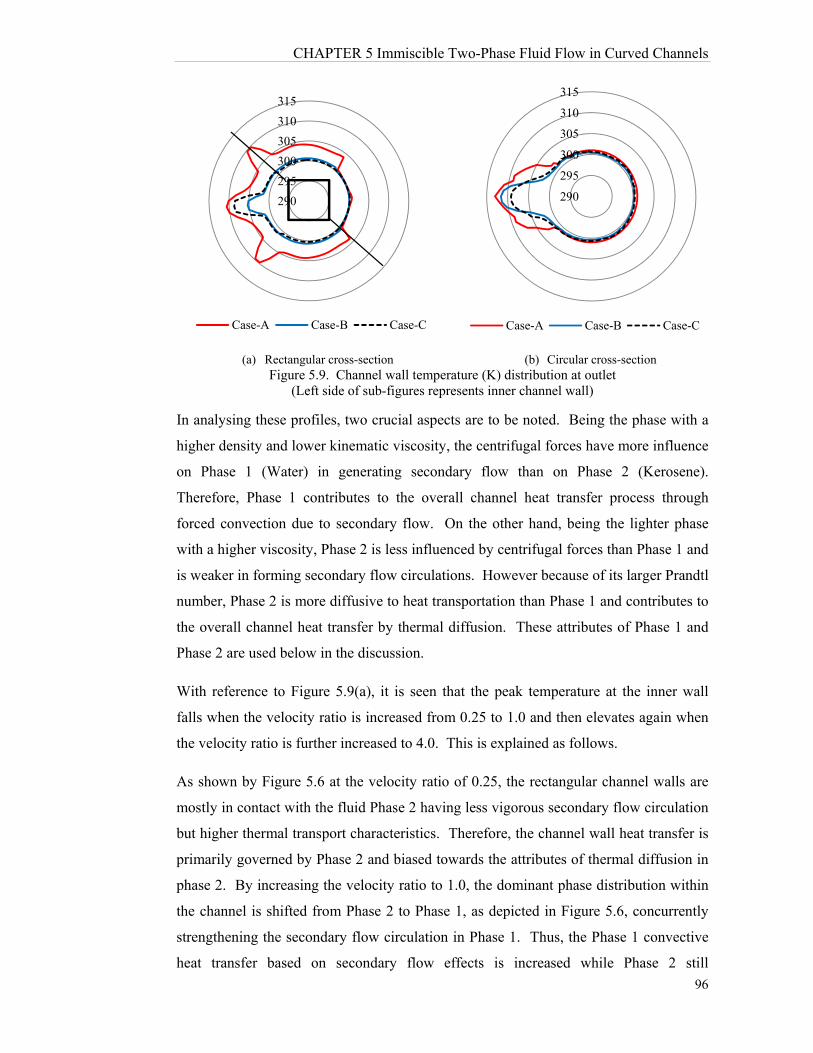
CHAPTER 5 Immiscible Two-Phase Fluid Flow in Curved Channels
96
(a) Rectangular cross-section (b) Circular cross-section Figure 5.9. Channel wall temperature (K) distribution at outlet
(Left side of sub-figures represents inner channel wall)
In analysing these profiles, two crucial aspects are to be noted. Being the phase with a
higher density and lower kinematic viscosity, the centrifugal forces have more influence
on Phase 1 (Water) in generating secondary flow than on Phase 2 (Kerosene).
Therefore, Phase 1 contributes to the overall channel heat transfer process through
forced convection due to secondary flow. On the other hand, being the lighter phase
with a higher viscosity, Phase 2 is less influenced by centrifugal forces than Phase 1 and
is weaker in forming secondary flow circulations. However because of its larger Prandtl
number, Phase 2 is more diffusive to heat transportation than Phase 1 and contributes to
the overall channel heat transfer by thermal diffusion. These attributes of Phase 1 and
Phase 2 are used below in the discussion.
With reference to Figure 5.9(a), it is seen that the peak temperature at the inner wall
falls when the velocity ratio is increased from 0.25 to 1.0 and then elevates again when
the velocity ratio is further increased to 4.0. This is explained as follows.
As shown by Figure 5.6 at the velocity ratio of 0.25, the rectangular channel walls are
mostly in contact with the fluid Phase 2 having less vigorous secondary flow circulation
but higher thermal transport characteristics. Therefore, the channel wall heat transfer is
primarily governed by Phase 2 and biased towards the attributes of thermal diffusion in
phase 2. By increasing the velocity ratio to 1.0, the dominant phase distribution within
the channel is shifted from Phase 2 to Phase 1, as depicted in Figure 5.6, concurrently
strengthening the secondary flow circulation in Phase 1. Thus, the Phase 1 convective
heat transfer based on secondary flow effects is increased while Phase 2 still
290
295
300
305
310
315
Case-A Case-B Case-C
290
295
300
305
310
315
Case-A Case-B Case-C

CHAPTER 5 Immiscible Two-Phase Fluid Flow in Curved Channels
97
contributing with some thermal diffusion. Hence, the higher overall heat flow reduces
the channel wall temperature. When the velocity ratio is further increased to 4.0, the
channel is primarily occupied by Phase 1 with a very small Phase 2 fluid circulation at
the inner wall, as shown by Figure 5.6. Therefore, the overall heat flow is very much
biased towards the forced convection brought about by Phase 1 secondary flow
circulation. This reduces the magnitude of overall channel heat flow, hence again
elevating the inner channel wall temperature at this velocity ratio of 4.0.
The circular channel wall temperature in Figure 5.9(b) behaves slightly different to the
rectangular channel temperature. In the circular channel, the peak temperature at the
inner wall continually falls when the velocity ratio is increased from 0.25 to 4.0. This is
because with the increased velocity ratio, the circular channel cross section geometry
readily deflects the Phase 1 secondary flow circulation in the vicinity of the outer wall
towards the inner wall, shifting Phase 2 away from the inner wall, as seen in Figure 5.6.
Consequently, the phase distribution within this geometry favours heavier Phase 1
reducing the influence from Phase 2 for all velocity ratios. Hence, the overall heat
transfer steadily increases with a continuing reduction in inner wall peak temperature.
5.5.7 Flow irreversibility analysis and thermal optimisation
Case-A Case-B Case-C
Figure 5.10. Bejan number contours indicating thermal irreversibility map at channel exit (Left side of sub-figures represents inner channel wall), 2m/W5000q
As Bejan Number contours, Figure 5.10 provides a Second Law thermal irreversibility
map of the flow situations discussed in Section 5.5.6. It is evident that, at low velocity
ratio, heat transfer-related irreversibility (red zones) is essentially confined to the inner
channel wall, signifying higher temperature differences in the fluid. This irreversibility
has a higher magnitude in circular ducts than in rectangular duct implying the latter
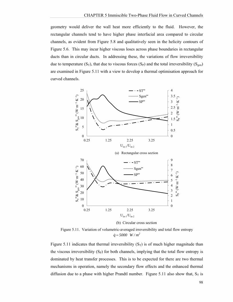
CHAPTER 5 Immiscible Two-Phase Fluid Flow in Curved Channels
98
geometry would deliver the wall heat more efficiently to the fluid. However, the
rectangular channels tend to have higher phase interfacial area compared to circular
channels, as evident from Figure 5.8 and qualitatively seen in the helicity contours of
Figure 5.6. This may incur higher viscous loses across phase boundaries in rectangular
ducts than in circular ducts. In addressing these, the variations of flow irreversibility
due to temperature (ST), that due to viscous forces (SP) and the total irreversibility (Sgen)
are examined in Figure 5.11 with a view to develop a thermal optimisation approach for
curved channels.
(a) Rectangular cross section
(b) Circular cross section
Figure 5.11. Variation of volumetric-averaged irreversibility and total flow entropy 2m/W5000q
Figure 5.11 indicates that thermal irreversibility (ST) is of much higher magnitude than
the viscous irreversibility (SP) for both channels, implying that the total flow entropy is
dominated by heat transfer processes. This is to be expected for there are two thermal
mechanisms in operation, namely the secondary flow effects and the enhanced thermal
diffusion due to a phase with higher Prandtl number. Figure 5.11 also show that, ST is
0
0.5
1
1.5
2
2.5
3
3.5
4
0
5
10
15
20
25
0.25 1.25 2.25 3.25
SP'''
(W·m
−3 ·
K−
1 )
ST'''&
Sge
n''' (
W·m
−3 ·
K−
1 )
Uin-1/Uin-2
ST'''
Sgen'''
SP'''
0
1
2
3
4
5
6
7
8
9
0
10
20
30
40
50
60
70
0.25 1.25 2.25 3.25
SP'''
(W·m
−3 ·
K−
1 )
ST'''&
Sge
n''' (
W·m
−3 ·
K−
1 )
Uin-1/Uin-2
ST'''
Sgen'''
SP'''

CHAPTER 5 Immiscible Two-Phase Fluid Flow in Curved Channels
99
minimised and SP reaches a peak when the phase velocity ratio approaches unity.
Attributable reasons for these behaviours are discussed below.
At velocity ratio of 1.0, helicity profiles in Figure 5.6 qualitatively indicate a higher
degree of contact between secondary circulations in Phases 1 and 2, which is vindicated
by Figure 5.8 as high phase interfacial area around this flow rate combination. Also, at
this velocity ratio, both phases have their highest intensity of secondary circulation, and
therefore the phase momentum transfer, as inferred from Figure 5.6. These two
mechanisms jointly cause the immiscible flow to experiences largest viscous loses at
this velocity ratio.
The minimisation of ST is a direct result of having the most favourable channel heat
transfer at the velocity ratio of 1.0. Under these flow conditions, Phases 1 and 2
contribute to the overall heat transfer through the most intense individual secondary
flow circulations, as judged from Figure 5.6 helicity profiles. At this velocity ratio, two
fluid phases are similarly distributed within the flow domain. This allows Phase 2 to
provide a significant contribution to the overall heat flow from thermal diffusion in
addition to its secondary flow-based forced convection. Consequently, both phase
jointly operate to increase the overall channel heat flow with the minimised thermal
irreversibility.
As evident from Figure 5.11, the total entropy, which is the sum of ST and SP, indicates
a minimum around the velocity ratio of 1.0. This minimum point represents the best
trade-off between opposing aspects of favourable thermal behaviour and adverse
viscous loses in the channel. Thus, it suggests an optimisation method for curved
channels carrying immiscible mixture of fluids, where the total flow irreversibility acts
as a useful and practical design parameter.
5.7. Summary
In this chapter, the fluid and thermal behaviour of a two-phase immiscible fluid mixture
was examined within both rectangular and circular curved channels. The unique flow
characteristics were assessed and explained by considering the effects from the
centrifugal forces due to channel curvature and the momentum transfer across the
phases. The channel convective heat transfer process is strongly influenced by the
CHAPTER 5 Immiscible Two-Phase Fluid Flow in Curved Channels
100
intensity of secondary flow as well as the non-uniform phase property distribution.
Extending this investigation of immiscible multi-phase flow, the next chapter examines
the two-phase flow through curved channels with additional mass transfer (evaporation)
at phase boundaries.
CHAPTER 6 Flow Boiling in Curved Channels
101
CHAPTER 6
CHAPTER 6 Flow Boiling In Curved Channels
6.1. Scope of chapter
This chapter focuses on study of a multi-phase flow having mass transfer through
interfaces and boiling heat transfer is discussed in details. Using Eulerian multi-phase
flow and wall heat partitioning approach and by assigning appropriate closures from
literature, unique influence of centrifugal force on phase rearrangement and accordingly
boiling heat transfer in curved ducts with different shapes of cross section is
investigated. In such term, straight and curved pipe are compared and effectiveness of
curvature is discussed regarding heat transfer enhancement and postponing temperature
increase in presence of high heat flux.
6.2. Introduction
Flow boiling and associated heat transfer characteristics are crucial design
considerations for thermal power generation and heat recovery systems. Through
decades of experimental work and numerical modelling, extensive knowledge base has
been developed in understanding the flow boiling regimes and thermal behaviour in
straight pipes. However, the two-phase flow behaviour in curved fluid passages
remains very much an unexplored area although such flow geometries are commonly
found as an integral part of many industrial heat transfer equipment of the kind, gas
turbine blades, boilers, helical heat exchangers and cooling system of centrifuges. In
heated ducts, the secondary flow affects the heat transfer characteristics by phase
rearrangement and special vortices structure. In previous chapters, single phase and
liquid-liquid flow through curved ducts, a significant degree of investigation has been
conducted to understand the intricate details of secondary flow interactions.
CHAPTER 6 Flow Boiling in Curved Channels
102
Experimental studies were associated with particular concerns regarding boiling such as
high working pressure, presences of dry-out, burnout and critical heat flux, boiling
investigation was so expensive and in some cases almost inaccessible. Besides,
investigations of flow boiling and thermal characteristics in curved passages remain so
much unexplored, in terms of numerical modelling.
Influence of source terms such as drag, lift, surface tension and extra turbulence
generation sources on boiling and corresponding characteristics are extensively studied.
Secondary flow, in multi-phase regimes, effects first on phase rearrangement where the
phase with higher density (i.e. liquid phase) experiences a higher centrifugal force and
moves toward outer side of curvature. The unsymmetrical resulting flow pattern will
fundamentally change the phase change regime (mass transfer from liquid to vapour
phase), heat transfer and other boiling characteristics in curved ducts.
This chapter represents an investigation on flow boiling within curved pipes, where pipe
curvature intrinsically produces secondary flow and hence, fundamentally different flow
characteristics as compared to straight pipes. For this, boiling process influenced by
secondary flow effects, the study develops a novel three-dimensional simulation
methodology based on a non-equilibrium model with Eulerian multi-phase approach. It
incorporates an incompressible multi-phase turbulent solver with k-ɛ model for
excellent integrity of predicted results and considerable computational advantage. The
model is tested for numerical stability and validated against reported experimental
results. The flow regimes and temperature fields are obtained for flow boiling in curved
pipes and compared with those in straight ducts with an analysis on observed
differences in fluid and thermal characteristics. The study evaluates individual wall
heat flux components that make up the overall heat transfer, namely that from liquid
evaporation, quenching, single phase liquid and single phase vapour. These are
effectively used for illustration and physical interpretation of the unique effects from
pipe curvature on the flow boiling process. The study also discusses the parametric
influence from liquid sub-cooling, wall heat flux and centrifugal forces on flow patterns
and, the onset of flow boiling in curved pipes along with the phase change and
associated heat transfer.
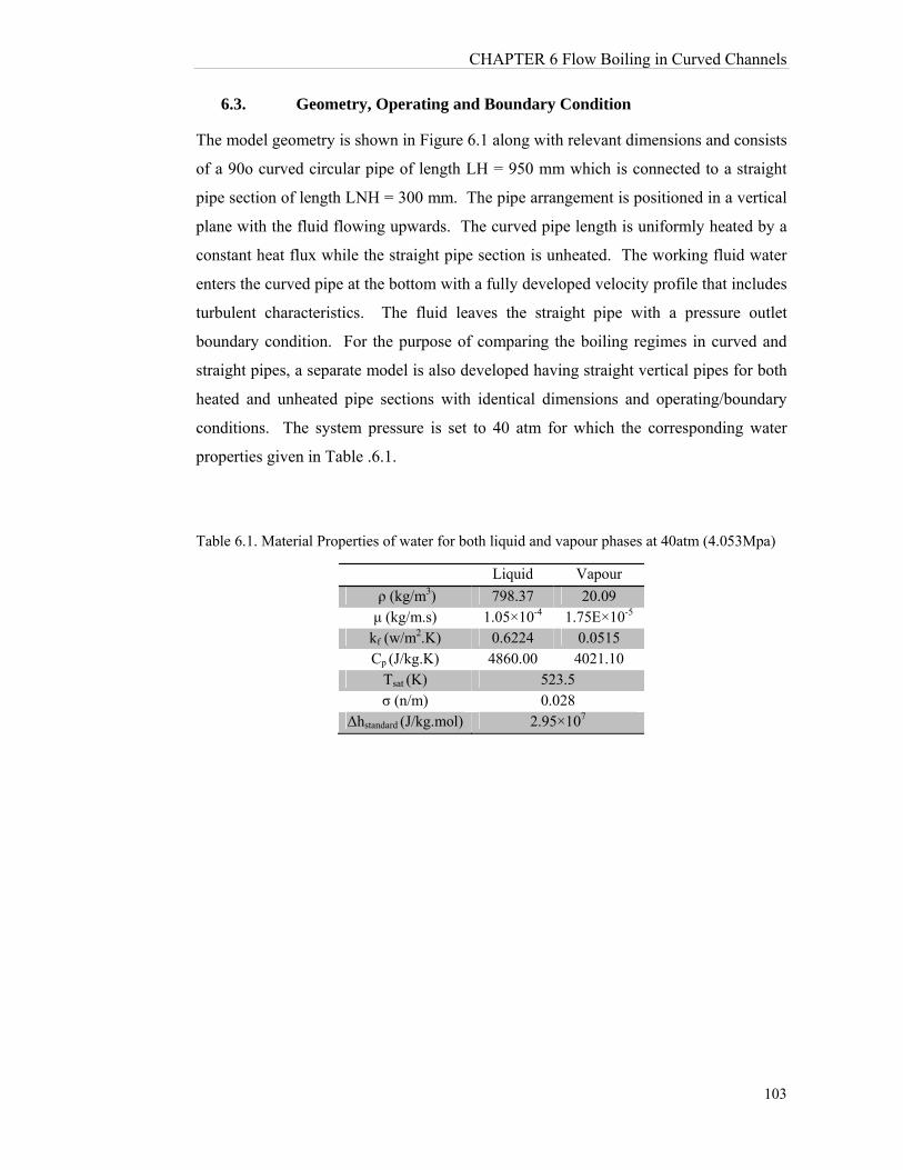
CHAPTER 6 Flow Boiling in Curved Channels
103
6.3. Geometry, Operating and Boundary Condition
The model geometry is shown in Figure 6.1 along with relevant dimensions and consists
of a 90o curved circular pipe of length LH = 950 mm which is connected to a straight
pipe section of length LNH = 300 mm. The pipe arrangement is positioned in a vertical
plane with the fluid flowing upwards. The curved pipe length is uniformly heated by a
constant heat flux while the straight pipe section is unheated. The working fluid water
enters the curved pipe at the bottom with a fully developed velocity profile that includes
turbulent characteristics. The fluid leaves the straight pipe with a pressure outlet
boundary condition. For the purpose of comparing the boiling regimes in curved and
straight pipes, a separate model is also developed having straight vertical pipes for both
heated and unheated pipe sections with identical dimensions and operating/boundary
conditions. The system pressure is set to 40 atm for which the corresponding water
properties given in Table .6.1.
Table 6.1. Material Properties of water for both liquid and vapour phases at 40atm (4.053Mpa)
Liquid Vapour
ρ (kg/m3) 798.37 20.09 μ (kg/m.s) 1.05×10⁻⁴ 1.75E×10-5
kf (w/m2.K) 0.6224 0.0515 Cp (J/kg.K) 4860.00 4021.10
Tsat (K) 523.5 σ (n/m) 0.028
Δhstandard (J/kg.mol) 2.95×10⁷
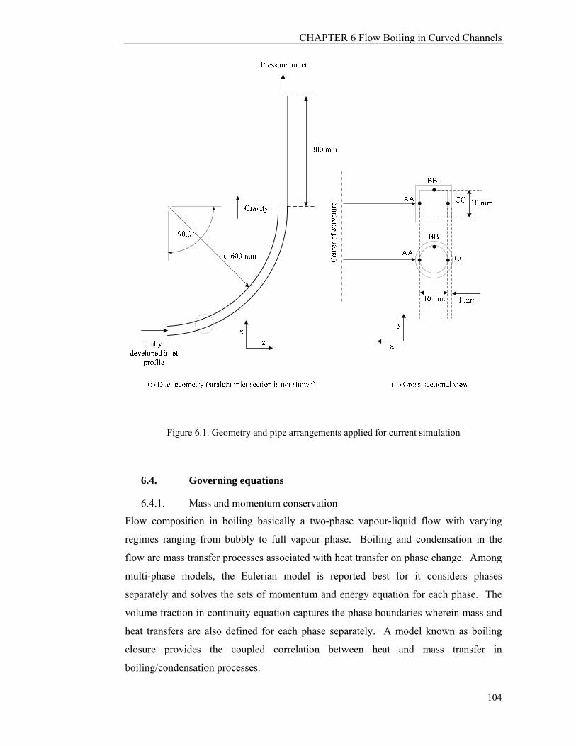
CHAPTER 6 Flow Boiling in Curved Channels
104
Figure 6.1. Geometry and pipe arrangements applied for current simulation
6.4. Governing equations
6.4.1. Mass and momentum conservation
Flow composition in boiling basically a two-phase vapour-liquid flow with varying
regimes ranging from bubbly to full vapour phase. Boiling and condensation in the
flow are mass transfer processes associated with heat transfer on phase change. Among
multi-phase models, the Eulerian model is reported best for it considers phases
separately and solves the sets of momentum and energy equation for each phase. The
volume fraction in continuity equation captures the phase boundaries wherein mass and
heat transfers are also defined for each phase separately. A model known as boiling
closure provides the coupled correlation between heat and mass transfer in
boiling/condensation processes.
CHAPTER 6 Flow Boiling in Curved Channels
105
For the explained configuration of model, continuity equation for the phase “q” is;
qppqqqq mmv
).( 6.1
The momentum and energy conservation equations;
liftbodyqqpqppqpq
TDpq
Dpqqqq
Tqqqqq
FFvmvm
FFgpv
..)(
qpqppqpqpqTqT
qfmqpqqq hmhmQTkTc .)( 2
6.2 (a)
6.2 (b)
bodyF
and liftF
are body and lift forces respectively while DpqF
and TDpqF
are drag force
and turbulence drift force. The effect of surface tension on pressure difference between
different phases and shape of boundaries are taken into account by approach suggested
by Brackbill et al [73].
6.4.2. Turbulence model
The viscous regime for tube boiling case is turbulent. q
. in equations 6.2 (a)&(b) is
Reynolds stress tensor and TqT. is temperature turbulence tensor which is in from of
generalized scalar turbulence tensor. These two terms make momentum and energy
equations coupled with two transport equations (depending on applied model) known as
turbulent closures. Among available turbulence closures k and k are widely
applied for multi-phase Eulerian model and reported to have a good consistency with
experimental results. Although k model solves turbulence equation for sub-layer
which improves wall turbulent characteristics, considering y confinements, cells
number significantly increases due to mesh refinement toward walls. Accordingly,
k with standard wall function could be applied as it represents a good compromise
of consistency with experimental results and demand for computational resource. k
RNG turbulence model, which is reported as a reliable model for bubbly flow [74] and
where RPI sub-model is used [51, 55], is adopted through following equations:
kmkk
tmmm SGkkv
)().( 2
SRk
CGk
Cv mkt
mmm ][)().(2
212
6.3(a)
6.3(b)
CHAPTER 6 Flow Boiling in Curved Channels
106
2kCmt
6.3(c)
where R is additional term related to mean stress and kG is turbulent kinetic energy
production rate, The RNG constants in equation 6.3 are,
42.1
1
1
C
k
68.1
3.1
2
C
0845.0C
6.4
while the bulk values for mixture domain are calculated as
2
1iiim
2
1
2
1
iii
iiii
m
v
v
6.5(a)
6.5(b)
Specific turbulence source terms for a turbulent bubbly regime (boiling case) are set
according to work of Troshko and Hassan [74] as
2)/(75.0 lvbvldragk vvdCS
lvbkdrag vvdSCS
)/(35.1
6.6(a)
6.6(b)
For the Eulerian model, the lift and virtual mass source terms are defined through
established approaches and corresponding correlations. However, the characteristics of
phase interaction require precise adjustment depending on the physical and numerical
condition for boiling to obtain stable solutions. These parameters to be considered are
briefly explained below.
6.4.3. Non-Equilibrium model
The current flow boiling simulation is based on a non-equilibrium model and is
formulated to alleviate a major modelling drawback in the RPI approach that assumes
thermal equilibrium between liquid and vapour phases. Similar to the RPI method, it
evaluates three wall heat partitioning components, namely the liquid convective,
quenching and evaporative heat fluxes. However for more realistic simulation, the
CHAPTER 6 Flow Boiling in Curved Channels
107
model also includes a fourth heat partitioning component to account for diffusive heat
flux of vapour bubble phase, thus removing the equilibrium assumption of vapour being
at saturation temperature adopted by the RPI method. The total wall heat flux is given
by the summation of the four terms as,
VEQLw qffqqqq ))(1()()( 11
6.7
The first three terms in Equation.6.7 are the heat flux components due to liquid
convection, cyclic-averaged transient heat transfer in liquid re-entering the wall region
after bubble detachment and the energy for evaporative phase change. )( vwvv TThq is
the diffusive heat flux from wall to vapour bubble that accounts for non-equilibrium
vapour phase. The function )(f is the local liquid volume fraction, which is defined
by,
4
)2.0(20
)2.0
(2
1
2
11
)(
l
le
f
Critl
Critl
6.8
Interfacial area ( iA ), which is important parameter due to its effect on drag force and
heat transfer process, is basically depends on bubble diameter; however, as it is affected
by bubble collision and it has to be modified. For current study interfacial area is
calculated as,
b
vvi D
A)1(6
6.9
In equation.6.2, drag force DpqF
for a bubbly boiling case is obtained from correlation
defined by Ishii and Zuber [75] as,
vlDliD
pq vvCA
F
8
6.10
where drag coefficient is determined by choosing minimum of viscous regime ( visDC )
and distorted regime ( disDC ) that are evaluated from,
CHAPTER 6 Flow Boiling in Curved Channels
108
)5.0.max(Re
)Re1.01(24 75.0
lb
bvisDC
)5.0,max(3
/)(2
l
vlbdisD
gdC
),min( disD
visDD CCC
6.11(a)
6.11(b)
6.11(c)
In the model, the wall region is partitioned into areas covered by either of bubbles or
liquid. Bubble diameter of vapour phase is adjusted according to a function suggested
by Kurul and Podowski [76] as follows,
00015.0
0001.000015.0
0015.0
Satb Td
5.13
5.130
0
Sub
Sub
Sub
T
T
T
6.12
The lift force liftF
in Equation 6.2-a is computed from the correlation developed by
Moraga et al [77] as,
)()( llvvlliftlift vvvCF
and
002.0
)103
exp()]36000
exp(2.012.0[
0767.0
7
liftC 5
53
3
109.1
109.1106
106
6.13(a)
6.13(b)
where ReReb . The bubble Reynolds number and bubble shear Reynolds numbers
which are used in Equation 6.13 a&b are defined as lvllbb vvd /Re and
lllb vd /Re 2 respectively.
vl
TDpq kF
6.14
As the vapour bubbles depart the wall, there would be a heat transfer from vapour
bubble to replacing liquid phase given by,

CHAPTER 6 Flow Boiling in Curved Channels
109
)( lsatslilt TThAq
6.15
where heat transfer coefficient slh is calculated from correlation suggested by Ranz-
Marshal [78] which is
)PrRe6.02( 33.05.0
b
lsl D
kh
6.16
Additionally interfacial heat transfer (heat transfer from superheated vapour to liquid) is
given by,
)(05.0 vsat
pvvvvt TT
cq
6.17
where time scale is assumed to be 0.05. Accordingly, the interfacial mass transfer which
directly depends on corresponding total heat transfer could be calculated as
fv
vtltlvlti h
qqmmm
6.18
Interfacial exchange parameters are briefly summarized in Table 6.1.
Table 6.4. Models applied for interactions between phases
Interaction term Applied Correlation Comment Reference
Drag Eq 6.10 & 6.11 Using bubble diameter Ishii and Zuber [75]
Lift Eq 6.13 Calculating coefficient Moraga et al. [77]
Heat transfer Eq 6.16 Vapour to liquid heat transfer
Ranz-Marshal [78]
Turbulence source terms
Eq 6.6 Generalized for bubbly regime
Troshko and Hassan [74]
Bubble Diameter Eq 6.12 Based on degree of sub-cooling
Kurnul and Podowski [76]
Numerical model simulates multi-phase flow and boiling has been briefly mentioned;
however, many well-established equations and closures, extensively available in
literature, have not been discussed here, as it is not necessary. Intricate and sensitive
case of boiling modelling is not limited with explained methodology and not only for
each type of modelling (e.g. pool boiling, nucleate boiling) is different numerical
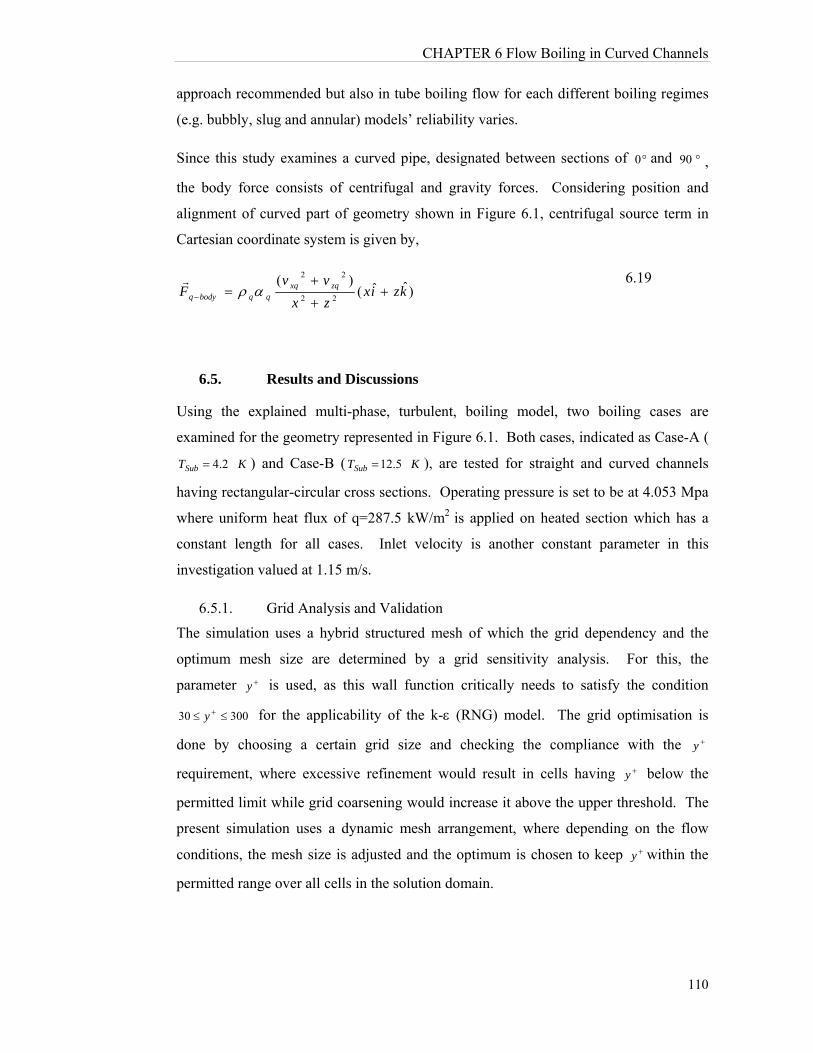
CHAPTER 6 Flow Boiling in Curved Channels
110
approach recommended but also in tube boiling flow for each different boiling regimes
(e.g. bubbly, slug and annular) models’ reliability varies.
Since this study examines a curved pipe, designated between sections of 0 and 90 ,
the body force consists of centrifugal and gravity forces. Considering position and
alignment of curved part of geometry shown in Figure 6.1, centrifugal source term in
Cartesian coordinate system is given by,
)ˆˆ()(
22
22
kzixzx
vvF zqxq
qqbodyq
6.19
6.5. Results and Discussions
Using the explained multi-phase, turbulent, boiling model, two boiling cases are
examined for the geometry represented in Figure 6.1. Both cases, indicated as Case-A (
KTSub 2.4 ) and Case-B ( KTSub 5.12 ), are tested for straight and curved channels
having rectangular-circular cross sections. Operating pressure is set to be at 4.053 Mpa
where uniform heat flux of q=287.5 kW/m2 is applied on heated section which has a
constant length for all cases. Inlet velocity is another constant parameter in this
investigation valued at 1.15 m/s.
6.5.1. Grid Analysis and Validation
The simulation uses a hybrid structured mesh of which the grid dependency and the
optimum mesh size are determined by a grid sensitivity analysis. For this, the
parameter y is used, as this wall function critically needs to satisfy the condition
30030 y for the applicability of the k- (RNG) model. The grid optimisation is
done by choosing a certain grid size and checking the compliance with the y
requirement, where excessive refinement would result in cells having y below the
permitted limit while grid coarsening would increase it above the upper threshold. The
present simulation uses a dynamic mesh arrangement, where depending on the flow
conditions, the mesh size is adjusted and the optimum is chosen to keep y within the
permitted range over all cells in the solution domain.
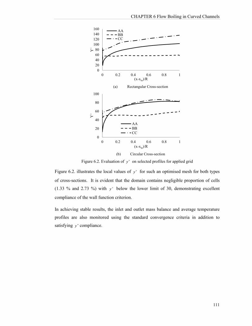
CHAPTER 6 Flow Boiling in Curved Channels
111
(a) Rectangular Cross-section
(b) Circular Cross-section
Figure 6.2. Evaluation of y on selected profiles for applied grid
Figure 6.2. illustrates the local values of y for such an optimised mesh for both types
of cross-sections. It is evident that the domain contains negligible proportion of cells
(1.33 % and 2.73 %) with y below the lower limit of 30, demonstrating excellent
compliance of the wall function criterion.
In achieving stable results, the inlet and outlet mass balance and average temperature
profiles are also monitored using the standard convergence criteria in addition to
satisfying y compliance.
020406080
100120140160
0 0.2 0.4 0.6 0.8 1
Y+
(x-xin)/R
AABBCC
0
20
40
60
80
100
0 0.2 0.4 0.6 0.8 1
Y+
(x-xin)/R
AABBCC
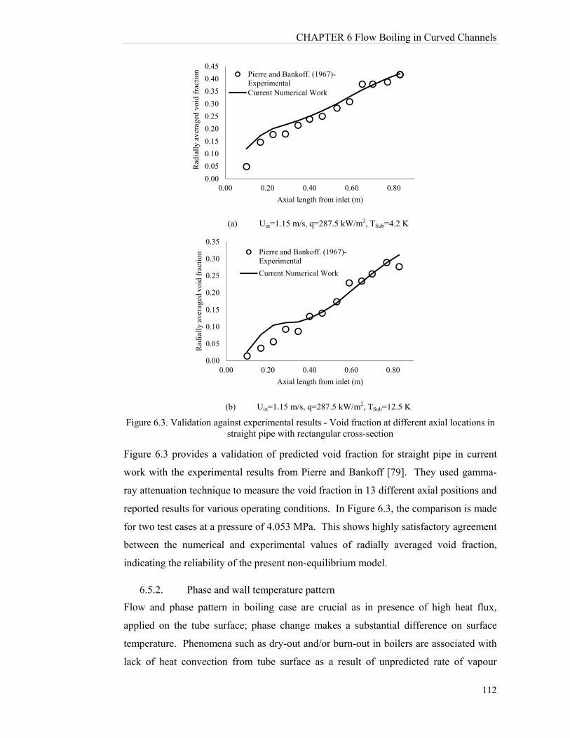
CHAPTER 6 Flow Boiling in Curved Channels
112
(a) Uin=1.15 m/s, q=287.5 kW/m2, TSub=4.2 K
(b) Uin=1.15 m/s, q=287.5 kW/m2, TSub=12.5 K
Figure 6.3. Validation against experimental results - Void fraction at different axial locations in straight pipe with rectangular cross-section
Figure 6.3 provides a validation of predicted void fraction for straight pipe in current
work with the experimental results from Pierre and Bankoff [79]. They used gamma-
ray attenuation technique to measure the void fraction in 13 different axial positions and
reported results for various operating conditions. In Figure 6.3, the comparison is made
for two test cases at a pressure of 4.053 MPa. This shows highly satisfactory agreement
between the numerical and experimental values of radially averaged void fraction,
indicating the reliability of the present non-equilibrium model.
6.5.2. Phase and wall temperature pattern
Flow and phase pattern in boiling case are crucial as in presence of high heat flux,
applied on the tube surface; phase change makes a substantial difference on surface
temperature. Phenomena such as dry-out and/or burn-out in boilers are associated with
lack of heat convection from tube surface as a result of unpredicted rate of vapour
0.00
0.05
0.10
0.15
0.20
0.25
0.30
0.35
0.40
0.45
0.00 0.20 0.40 0.60 0.80R
adia
lly
aver
aged
voi
d fr
acti
onAxial length from inlet (m)
Pierre and Bankoff. (1967)-ExperimentalCurrent Numerical Work
0.00
0.05
0.10
0.15
0.20
0.25
0.30
0.35
0.00 0.20 0.40 0.60 0.80
Rad
iall
y av
erag
ed v
oid
frac
tion
Axial length from inlet (m)
Pierre and Bankoff. (1967)-Experimental
Current Numerical Work

CHAPTER 6 Flow Boiling in Curved Channels
113
production. Additionally, boiling is used as a heat transfer enhancement technique:
extra heat could be removed by evaporation mechanism as the extra heat is spent on
latent heat during phase-change procedure. Therefore, for taking extreme advantages of
boiling on surface heat transfer, flow pattern should be optimized with prospective of
maximizing quenching heat transfer as well as evaporative heat transfer on the surface.
The unique influence of centrifugal force on phase arrangement and vortices structure is
shown in Figure 6.4. Bubble diameter, as pointed in numerical approach, has small
dimensions as compared to grid size and is considered as a scalar for each cell, on basis
of which other related parameter would be calculated. Hence, volume fraction between
zero and one resulted from Eulerian approach is justified both physical and numerically.
In curved pipe, the void fraction pattern depicts a marked deviation from the “axi-
symmetry” observed for straight pipes. It is seen that, in the presence of pipe flow
curvature, the vapour phase is highly concentrated closer to the inner wall (left of
diagram) while the liquid phase is displaced towards the outer pipe wall (right of
diagram). This is because, the centrifugal forces generated by pipe curvature impart
more inertia effect on the heavier liquid component, pushing it outwards.
Consequently, the void fraction distribution is radially uneven over the pipe cross
section unlike in straight pipe. This creates favourable implications on the two-phase
boiling heat transfer process, as explained below.
In straight pipe, radially even vapour distribution acts as a uniform thermal barrier for
wall heat flow into the liquid. In curved pipe, the void fraction profile biased towards
the inner wall improves heat transfer process in two ways. Firstly, it makes the liquid
component to have a higher circumferential contact with the heated wall, thus
increasing the potential for liquid evaporation. Secondly, at pipe wall areas with thinner
vapour distribution, thermal resistance to heat flow from the wall to liquid is reduced.
Combination of these mechanisms results in improved overall flow boiling heat transfer
rate.

CHAPTER 6 Flow Boiling in Curved Channels
114
Ldv=0.1
Ldv=0.285
Ldv=0.47
Ldv=0.7
Ldv=0.83
(a) Rectangular (b) Circular
Figure 6.4. Void fraction and dimensionless helicity contours on selected positions (outer wall is located right-side)
As evident in the void fraction contours, qualitative arrangement of phases for
rectangular and circular cross section is almost similar and obviously interfacial area is
not as sharp as immiscible flow case. Since bubble and liquid elements of flow, due to
large density difference, would experience a high difference in centrifugal force, the
separation starts from curvature inception. Accordingly, throughout channel the vapour
phase remains in area closer to inner wall, liquid phase stocks at outer wall and
nucleation sites would largely form on the side walls. The main reason for similar flow
and phase pattern for different shapes of cross section is placement of phases on to sides
of cross section where no cross-sectional phase takeover happens all through channel.
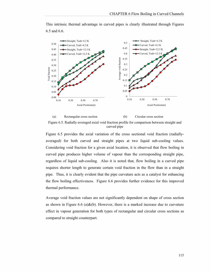
CHAPTER 6 Flow Boiling in Curved Channels
115
This intrinsic thermal advantage in curved pipes is clearly illustrated through Figures
6.5 and 6.6.
(a) Rectangular cross section (b) Circular cross section
Figure 6.5. Radially-averaged axial void fraction profile for comparison between straight and curved pipe
Figure 6.5 provides the axial variation of the cross sectional void fraction (radially-
averaged) for both curved and straight pipes at two liquid sub-cooling values.
Considering void fraction for a given axial location, it is observed that flow boiling in
curved pipe produces higher volume of vapour than the corresponding straight pipe,
regardless of liquid sub-cooling. Also it is noted that, flow boiling in a curved pipe
requires shorter length to generate certain void fraction in the flow than in a straight
pipe. Thus, it is clearly evident that the pipe curvature acts as a catalyst for enhancing
the flow boiling effectiveness. Figure 6.6 provides further evidence for this improved
thermal performance.
Average void fraction values are not significantly dependent on shape of cross section
as shown in Figure 6.6 (a)&(b). However, there is a marked increase due to curvature
effect in vapour generation for both types of rectangular and circular cross sections as
compared to straight counterpart.
0.00
0.05
0.10
0.15
0.20
0.25
0.30
0.35
0.40
0.45
0.50
0.10 0.30 0.50 0.70
Voi
d fr
actio
n
Axial Position(m)
Straight, Tsub=4.2 K
Curved, Tsub=4.2 K
Straight, Tsub=12.5 K
Curved, Tsub=12.5 K
0
0.05
0.1
0.15
0.2
0.25
0.3
0.35
0.4
0.45
0.5
0.10 0.30 0.50 0.70
Ave
rage
voi
d fr
acti
on
Axial Position(m)
Straight, Tsub=4.2 K
Curved, Tsub=4.2 K
Straight, Tsub=12.5 K
Curved, Tsub=12.5 K
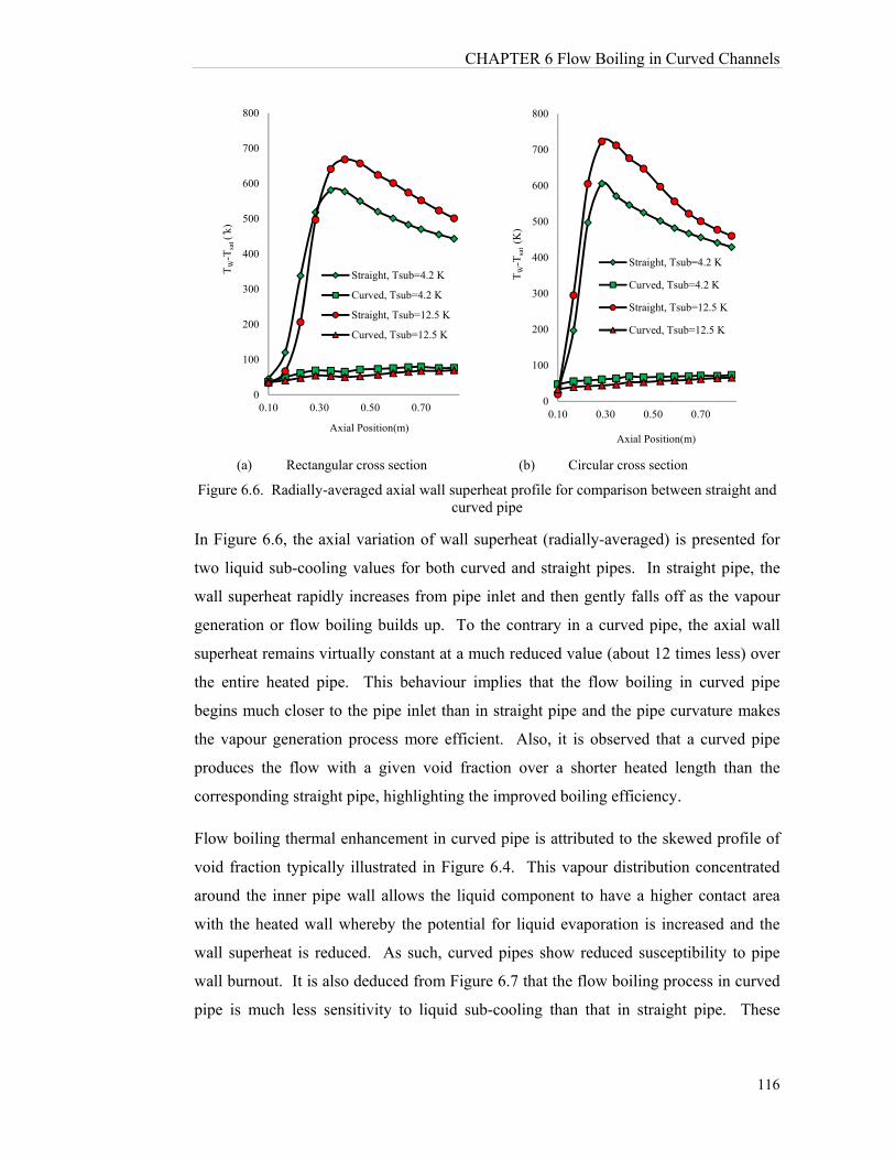
CHAPTER 6 Flow Boiling in Curved Channels
116
(a) Rectangular cross section (b) Circular cross section
Figure 6.6. Radially-averaged axial wall superheat profile for comparison between straight and curved pipe
In Figure 6.6, the axial variation of wall superheat (radially-averaged) is presented for
two liquid sub-cooling values for both curved and straight pipes. In straight pipe, the
wall superheat rapidly increases from pipe inlet and then gently falls off as the vapour
generation or flow boiling builds up. To the contrary in a curved pipe, the axial wall
superheat remains virtually constant at a much reduced value (about 12 times less) over
the entire heated pipe. This behaviour implies that the flow boiling in curved pipe
begins much closer to the pipe inlet than in straight pipe and the pipe curvature makes
the vapour generation process more efficient. Also, it is observed that a curved pipe
produces the flow with a given void fraction over a shorter heated length than the
corresponding straight pipe, highlighting the improved boiling efficiency.
Flow boiling thermal enhancement in curved pipe is attributed to the skewed profile of
void fraction typically illustrated in Figure 6.4. This vapour distribution concentrated
around the inner pipe wall allows the liquid component to have a higher contact area
with the heated wall whereby the potential for liquid evaporation is increased and the
wall superheat is reduced. As such, curved pipes show reduced susceptibility to pipe
wall burnout. It is also deduced from Figure 6.7 that the flow boiling process in curved
pipe is much less sensitivity to liquid sub-cooling than that in straight pipe. These
0
100
200
300
400
500
600
700
800
0.10 0.30 0.50 0.70
TW
-Tsa
t ( ̊k
)
Axial Position(m)
Straight, Tsub=4.2 K
Curved, Tsub=4.2 K
Straight, Tsub=12.5 K
Curved, Tsub=12.5 K
0
100
200
300
400
500
600
700
800
0.10 0.30 0.50 0.70
TW
-Tsa
t (K
)
Axial Position(m)
Straight, Tsub=4.2 K
Curved, Tsub=4.2 K
Straight, Tsub=12.5 K
Curved, Tsub=12.5 K
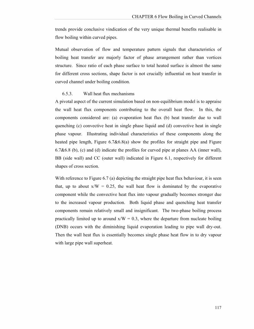
CHAPTER 6 Flow Boiling in Curved Channels
117
trends provide conclusive vindication of the very unique thermal benefits realisable in
flow boiling within curved pipes.
Mutual observation of flow and temperature pattern signals that characteristics of
boiling heat transfer are majorly factor of phase arrangement rather than vortices
structure. Since ratio of each phase surface to total heated surface is almost the same
for different cross sections, shape factor is not crucially influential on heat transfer in
curved channel under boiling condition.
6.5.3. Wall heat flux mechanisms
A pivotal aspect of the current simulation based on non-equilibrium model is to appraise
the wall heat flux components contributing to the overall heat flow. In this, the
components considered are: (a) evaporation heat flux (b) heat transfer due to wall
quenching (c) convective heat in single phase liquid and (d) convective heat in single
phase vapour. Illustrating individual characteristics of these components along the
heated pipe length, Figure 6.7&6.8(a) show the profiles for straight pipe and Figure
6.7&6.8 (b), (c) and (d) indicate the profiles for curved pipe at planes AA (inner wall),
BB (side wall) and CC (outer wall) indicated in Figure 6.1, respectively for different
shapes of cross section.
With reference to Figure 6.7 (a) depicting the straight pipe heat flux behaviour, it is seen
that, up to about x/W = 0.25, the wall heat flow is dominated by the evaporative
component while the convective heat flux into vapour gradually becomes stronger due
to the increased vapour production. Both liquid phase and quenching heat transfer
components remain relatively small and insignificant. The two-phase boiling process
practically limited up to around x/W = 0.3, where the departure from nucleate boiling
(DNB) occurs with the diminishing liquid evaporation leading to pipe wall dry-out.
Then the wall heat flux is essentially becomes single phase heat flow in to dry vapour
with large pipe wall superheat.
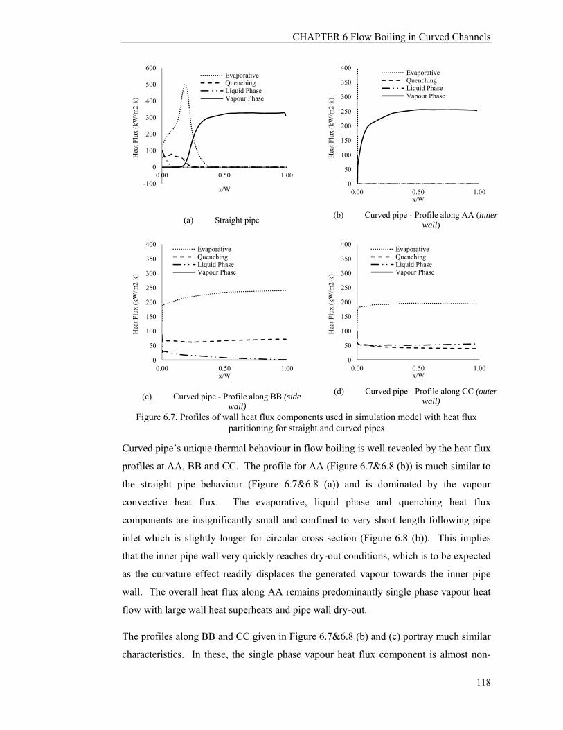
CHAPTER 6 Flow Boiling in Curved Channels
118
(a) Straight pipe
(b) Curved pipe - Profile along AA (inner wall)
(c) Curved pipe - Profile along BB (side wall)
(d) Curved pipe - Profile along CC (outer wall)
Figure 6.7. Profiles of wall heat flux components used in simulation model with heat flux partitioning for straight and curved pipes
Curved pipe’s unique thermal behaviour in flow boiling is well revealed by the heat flux
profiles at AA, BB and CC. The profile for AA (Figure 6.7&6.8 (b)) is much similar to
the straight pipe behaviour (Figure 6.7&6.8 (a)) and is dominated by the vapour
convective heat flux. The evaporative, liquid phase and quenching heat flux
components are insignificantly small and confined to very short length following pipe
inlet which is slightly longer for circular cross section (Figure 6.8 (b)). This implies
that the inner pipe wall very quickly reaches dry-out conditions, which is to be expected
as the curvature effect readily displaces the generated vapour towards the inner pipe
wall. The overall heat flux along AA remains predominantly single phase vapour heat
flow with large wall heat superheats and pipe wall dry-out.
The profiles along BB and CC given in Figure 6.7&6.8 (b) and (c) portray much similar
characteristics. In these, the single phase vapour heat flux component is almost non-
-100
0
100
200
300
400
500
600
0.00 0.50 1.00
Hea
t Flu
x (k
W/m
2-k)
x/W
EvaporativeQuenchingLiquid PhaseVapour Phase
0
50
100
150
200
250
300
350
400
0.00 0.50 1.00
Hea
t Flu
x (k
W/m
2-k)
x/W
EvaporativeQuenchingLiquid PhaseVapour Phase
0
50
100
150
200
250
300
350
400
0.00 0.50 1.00
Hea
t Flu
x (k
W/m
2-k)
x/W
EvaporativeQuenchingLiquid PhaseVapour Phase
0
50
100
150
200
250
300
350
400
0.00 0.50 1.00
Hea
t Flu
x (k
W/m
2-k)
x/W
EvaporativeQuenchingLiquid PhaseVapour Phase
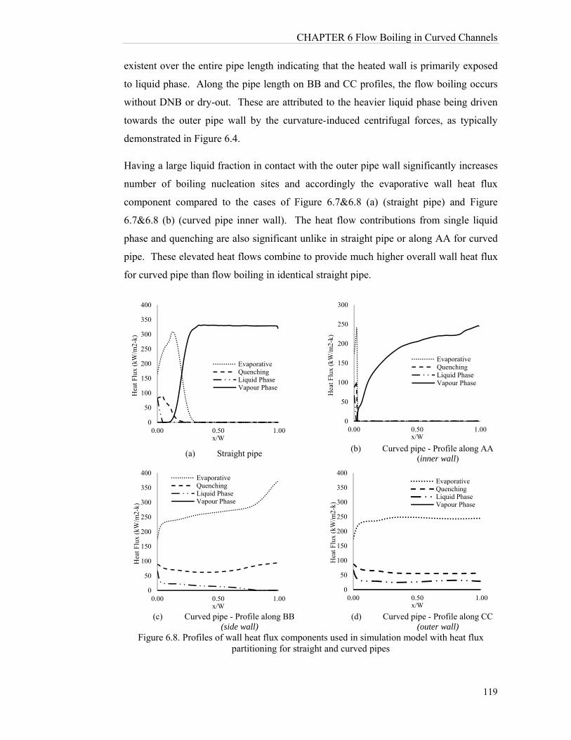
CHAPTER 6 Flow Boiling in Curved Channels
119
existent over the entire pipe length indicating that the heated wall is primarily exposed
to liquid phase. Along the pipe length on BB and CC profiles, the flow boiling occurs
without DNB or dry-out. These are attributed to the heavier liquid phase being driven
towards the outer pipe wall by the curvature-induced centrifugal forces, as typically
demonstrated in Figure 6.4.
Having a large liquid fraction in contact with the outer pipe wall significantly increases
number of boiling nucleation sites and accordingly the evaporative wall heat flux
component compared to the cases of Figure 6.7&6.8 (a) (straight pipe) and Figure
6.7&6.8 (b) (curved pipe inner wall). The heat flow contributions from single liquid
phase and quenching are also significant unlike in straight pipe or along AA for curved
pipe. These elevated heat flows combine to provide much higher overall wall heat flux
for curved pipe than flow boiling in identical straight pipe.
(a) Straight pipe (b) Curved pipe - Profile along AA
(inner wall)
(c) Curved pipe - Profile along BB (side wall)
(d) Curved pipe - Profile along CC (outer wall)
Figure 6.8. Profiles of wall heat flux components used in simulation model with heat flux partitioning for straight and curved pipes
0
50
100
150
200
250
300
350
400
0.00 0.50 1.00
Hea
t Flu
x (k
W/m
2-k)
x/W
EvaporativeQuenchingLiquid PhaseVapour Phase
0
50
100
150
200
250
300
0.00 0.50 1.00
Hea
t Flu
x (k
W/m
2-k)
x/W
EvaporativeQuenchingLiquid PhaseVapour Phase
0
50
100
150
200
250
300
350
400
0.00 0.50 1.00
Hea
t Flu
x (k
W/m
2-k)
x/W
EvaporativeQuenchingLiquid PhaseVapour Phase
0
50
100
150
200
250
300
350
400
0.00 0.50 1.00
Hea
t Flu
x (k
W/m
2-k)
x/W
EvaporativeQuenchingLiquid PhaseVapour Phase

CHAPTER 6 Flow Boiling in Curved Channels
120
From the above comparative analysis with straight pipe, it is recognised that the curved
pipe geometry brings about the secondary flow fluid interaction to the flow boiling
process that will delay the departure from nucleate boiling and dry-out at the wall while
enhancing the wall heat transfer and reducing the wall superheat. In view of dry-out
and burn-out issues associated with boilers tubes, the identified thermal benefits of flow
boiling within curved pipe geometry are practically significant and meaningful for
sustainable energy resource usage.
Rectangular and circular cross sections have been compared in in term of heat transfer
components at the selected cross sections where the emphasis is on effect of curvature.
On the given profiles rectangular cross section found to be more effective in vapour
generation whereas circular cross section has greater evaporative and quenching heat
flux. Such investigation could be extended along with vortices structure assessment,
especially to capture effect of sharp corners on temperature rise-up in rectangular cross
sections which requires a more detailed analysis.
6.6. Summary
In this chapter, a numerical flow boiling model in curved pipe has been developed
incorporating non-equilibrium model with wall heat partitioning, Eulerian multi-phase
approach and k-ɛ turbulence model. The model produces consistent and stable results
that are validated against experimental values with a good agreement. The simulation
identifies the unique features of flow boiling within curved pipes, where the secondary
flow from arising from curvature-induced centrifugal effects significantly alters the
boiling regimes and heat transfer characteristics compared to straight pipes.
This numerical analysis concludes that the secondary flow interaction from pipe
curvature has intrinsic ability to enhance the thermal effectiveness of flow boiling
process by increasing the wall heat flux rates, reducing the wall superheat, delaying the
departure from nucleate boiling (DNB) and significantly lowering the possibilities for
wall dry-out. Compared to straight pipes, the flow boiling in curved pipes can produce
vapour at a higher rate with a shorter pipe length and without much sensitivity to liquid
sub-cooling.
CHAPTER 6 Flow Boiling in Curved Channels
121
Average values of boiling characteristics have been found insensitive against shape of
cross section; however, phenomenon such as local temperature increase is observed as a
result of vortices structure which could be analysed with more details.
CHAPTER 7 Conclusions
122
CHAPTER 7
CHAPTER 7 Conclusions
7.1. Research Summary and Significant Outcomes
The study presented in this thesis carried out an extensive review of published literature
on the aspects of secondary flow behaviour in single and multi-phase fluid flow through
curved channels and the associated heat transfer processes. It identified that, the
available simulation methods have yet to provide realistic representations of the
complex secondary flow features and their impact on thermal characteristics. Also, the
parametric influences of duct geometrical and flow variables remain largely unexplored
and poorly understood. Decisive and reliable criteria are presently not at disposal for
accurate prediction and identification of Dean vortex generation and the onset of Dean’s
Instability in curved channel flow fields. Most investigations have been primarily
confined to single-phase flow through curved rectangular ducts while the flow
behaviours within elliptical and circular geometries have received insignificant priority
and attention. Analyses with immiscible and boiling two-phase flow through curved
channels are rarer or non-existent. Very few attempts have been made in reported
literature to establish suitable techniques to optimise thermal behaviour of fluid flow
through heated curved channels in view of practical design requirements. Addressing
above key limitations, the study presented in the thesis carefully formulated its research
scope, objectives and methodology and, carried out an extensive investigation of which
details were presented in previous chapters covering the single phase, immiscible two-
phase and two-phase boiling fluid flows through curved channels.
(a) Single-Phase fluid flow in curved channels
Making a significant contribution to improve the current simulation methodologies for
single-phase fluid flow, the study developed an advanced three-dimensional numerical
model based on (helicity) vortex structures, which is more compatible and congruent
with the spiralling fluid motion of secondary flow. In this, necessary User Defined

CHAPTER 7 Conclusions
123
Functions (UDF) were formulated and integrated into the computational fluid dynamics
software package FLUENT as a solver. The adapted modelling approach provides
much compliant tracking of vortex flow paths and, very effective capturing of intricate
details of secondary vortices, supported by the use of a curvilinear mesh arrangement.
The chosen meshes were shown to be more accurate for representing steep flow profiles
in a variety of channel geometries attempted. The model was successfully tested for its
consistency and prediction accuracy and, validated against the available experimental
data to confirm the realisable modelling improvements over the previous models.
In fulfilling a critical analytical need for this field of research, the study formulated two
intuitive approaches as a tool for detecting the onset of Dean Instability. One approach
using an assigned dimensionless helicity threshold was realised to be universally
applicable without fail to all channel shapes and flow conditions, and provided the
flexibility to manage the detection accuracy versus computational demand. The second
approach using the outer wall pressure gradient profile was found to be extremely useful
to obtain prompt qualitative indication of the vortex generation potential. Both
techniques are similarly applicable for rectangular geometries while the pressure
gradient method was found to over-predict the conditions for Dean’s Instability in
circular and elliptical ducts. These two criteria are far reliable and accurate than any
other reported method in literature while having the provision for performing directly
within the computational process.
The single-phase simulation model successfully predicted the fluid flow behaviour
within rectangular, elliptical and circular channels, accurately and consistently
identifying the onset of Dean’s Instability. It precisely captured the centrifugal effects
from fluid flow rate, the geometrical influence from channel shape and aspect ratio, and
the buoyancy effects from channel wall heating. As such, the study provides
unprecedented details on parametric influences with a variety of channel geometries
compared to the published work.
The study also developed a useful thermal optimisation technique for heated curved
channel flows. Evaluating the individual contributions to flow irreversibilites from heat
transfer and fluid viscosity, this proposed technique identified a point of inflection for
the overall entropy as practically the best possible “trade-off” between the highest
achievable thermal benefits with the least viscous penalty for curved channel flows.

CHAPTER 7 Conclusions
124
(b) Immiscible Two-Phase fluid flow in curved channels
In view of the relevance to industrial process applications, the simultaneous flow of two
non-mixing fluid components within heated curved circular channels was examined.
The study developed a new three-dimensional simulation based on Volume of Fraction
(VOF) specifically for this type of two-phase flow in circular channel. Suitable mesh
arrangements were considered with compatibilities for near-wall turbulence models and
capabilities to capture the formations of immiscible fluid phases.
The model was tested for consistency and accuracy. It successfully predicted the unique
features arising from the interaction between the centrifugal forces and the momentum
transfer between phases. These interactions lead to the formation of secondary vortices
simultaneously in each fluid phase. The intensity of phase vortices primarily changed
with the velocity ratio between phases, where the flow patterns were dominated by
heavier phase at high velocity ratio and by lighter phase at low velocity ratio. As a
useful design feature for certain reactive flow processes, it was observed that
immiscible flow mixture in a curved channel is able to provide 3.5 times more
interfacial area between phases than the corresponding such flows in straight pipes.
It was found in immiscible flows, thermal characteristics are sustained by both forced
convection and heat diffusion processes. The former is more contributed by the fluid
phase with the higher density for its centrifugal action while the latter by the phase with
the higher Prandtl number for its better thermal transport ability. Following the same
approach as for single-phase flow, a similar thermal optimisation scheme considering
individual phase irreversibilities were successfully developed for this immiscible two-
phase fluid flow through curved channels.
A numerical investigation for immiscible two-phase fluid flow in curved channels as
presented in this study is not currently reported in the published literature.
(c) Two-Phase flow boiling in curved channels
The single-phase three-dimensional simulation model was modified and extended to
describe the two-phase flow boiling processes in curved ducts. This model represents a
significant improvement over the previous methods for it applied a realistic approach of
wall heat partitioning techniques at the vapour and liquid interfaces. With this, it
modelled both mass and heat transfer processes across phase boundaries and included

CHAPTER 7 Conclusions
125
the interfacial momentum transfer. Thus, this new approach represents the most
accurate to-date in terms of physical mechanisms involved among the two-phase flow
models for this type of fluid flow with boiling. The model was verified for its
consistency and accuracy and, validated against the available experimental data.
The model successfully predicted the unique phase distribution characteristics and
boiling heat transfer process in circular channels. It identified that the flow boiling
within curved channels is far more efficient than that within straight ducts. In curved
channels, wall temperature is significantly reduced while producing higher fraction of
vapour than in a corresponding straight duct due to the unique liquid phase distribution
driven by the centrifugal forces.
As an overall conclusion, the study presented in this thesis delivers research outcomes
that significantly advance the current state of knowledge through new numerical
simulation methodologies for multi-phase fluid flow in heated curved channels of
various geometries, novel detection methods of Dean’s Instability and clearer
understanding of secondary flow behaviour in multi-phase flows and associated heat
transfer processes.
7.2. Possible Future Research directions
(i) Numerical modelling
The current study is so extensive it seems to have exhausted almost all directions for
further numerical work on single-phase flow in curved channels. However, there are
more possibilities in multi-phase flow studies. The numerical model developed for the
flow boiling heat transfer investigates unique behaviour of phase formation and heat
transfer in a limited range of heat flux and Reynolds number. Parametric analysis can
be extended for a wider range to observe the influence of various parameters. It would
be challenging and interesting to examine the flow behaviour near the critical heat flux
condition, where special care may be needed. It would be useful to consider the sub-
models suggested by Tentner et al. [80] and Loilev et al. [81] for improved accuracy.
(ii) Experimental work
The vortex-based numerical analysis developed in this study could be verified through
the experimental velocity fields. Flow visualisation and quantitative assessment of the

CHAPTER 7 Conclusions
126
secondary flow vortices are a major challenge because of the intrusive nature of
experimental probes such as hot-wire anemometer. Promising optical methods are LDA
(or LDV), LIF and PIV where it would be possible to obtain the necessary data sets for
the complex flow fields in curved channels. Recent technical development is Stereo-
PIV which provides sophisticated real-time fluid field analysis for measuring three-
dimensional velocity fields. Such data set would be useful for combining with the
helicity threshold method for verifying the formation process of secondary vortex
structures and Dean’s Instability. Currently, such data do not exist.
Obtaining the flow temperature profiles in curved channels is a challenge that has not
been sufficiently addressed. Planar-LIF methods would allow such complex
measurements of thermal fields in curved channels for quantitative local temperatures,
permitting confident numerical validations.
Application of optical method for boiling case might be challenging and needs special
consideration since the measuring systems require tolerating high heat fluxes of the
order of 30-800 kW/m2, where maintaining wall transparency would be an issue.
However, it may be possible to use traditional approaches suggested by Pierre and
Bankoff [79] to obtain some elementary parameters such as volume fraction or surface
temperature for boiling heat transfer in curved channels.
References
127
References
1. J. Eustice, Flow of Water in Curved Pipes, Proceedings of the Royal Society of
London. Series A, 84 (568) (1910), pp. 107-118.
2. J, Eustice, Experiments on Stream-Line Motion in Curved Pipes, Proceedings of
the Royal Society of London. Series A,.85(576) (1911), pp. 119-131.
3. W.R. Dean, Note on the motion of fluid in a curved pipe, Philosophical Magazine
Series 7, Vol.4:20 (1927), pp 208-223.
4. W.R. Dean, The stream-line motion of fluid in a curved pipe, Philosophical
Magazine Series 7, 5:30 (1927), pp 673-695.
5. W. R. Dean, Fluid Motion in a Curved Channel, Proceedings of the Royal Society
of London. Series A, 121 (787) (1928), pp. 402-420. recommend
6. C. M. White, Streamline Flow through Curved Pipes, Proceedings of the Royal
Society of London. Series A, 123 (792) (1929), pp. 645-663.
7. J.A. Baylis, Experiments on laminar flow in curved channels of square section,
Journal of Fluid Mechanics, 48(3) (1971), pp 417–422.
8. J.A.C. Humphrey, A.M.K. Taylor, J.H. Whitelaw, Laminar flow in a square duct of
strong curvature, Journal of Fluid Mechanics, 83 (1977), pp 509–527.
9. K.C. Cheng, J. Nakayama, M. Akiyama, Effect of finite and infinite aspect ratios on
flow patterns in curved rectangular channels, in: Flow Visualization International
Symposium, Tokyo, October 1977, p. 181.
10. Ghia, K.N., Sokhey, J.S., Laminar incompressible viscous flow in curved ducts of
rectangular cross-section, Journal of Fluids Engineering, 99 (1977), pp. 640–648.
11. M. M. Enayet, M. M. Gibson and M. Yianneskis, Measurements of turbulent
developing flow in a moderately curved square duct, International journal of heat
and fluid flow, Vol 3 (4) (1982), pp 221-224.
12. Sugiyama, Taro Hayashi, Koji Yamazaki, Flow Characteristics in the Curved
Rectangular Channels, Bullletin of JSME, 26(216) (1983), pp 532-552.
13. Dong, Z.F., and Ebadian, Numerical analysis of laminar flow in curved elliptic
ducts, Journal of Fluid Engineering, 113 (1991), pp. 555-562.
14. T. Chandratilleke, Nursubiyakto. "Numerical prediction of secondary flow and
convective heat transfer in externally heated curved rectangular ducts."
International Journal of Thermal sciences, 42(2002), pp. 187–198.
References
128
15. H. Fellouah, C. C., A. Ould El Moctar, H. Peerhossaini "A criterion for detection of
the onset of Dean instability in Newtonian fluids." European Journal of Mechanics
B/Fluids, l25 (2006), pp 505–531.
16. L. Helin, L. Thais, G. Mompean, Numerical simulation of visco-elastic Dean
vortices in a curved duct, Journal of Non-Newtonian Fluid Mechanics, 156 (2009),
pp 84-94.
17. H. Fellouaha, C. Castelainb, A. Ould-El-Moctarb, H. Peerhossaini, The Dean
instability in power-law and Bingham fluids in a curved rectangular duct, J. Non-
Newtonian Fluid Mech, 165 (2010), pp. 163–173.
18. K. C. Cheng and Mitsunobu Akiyama, Laminar forced convection heat transfer in
curved rectangular channels, international of heat and mass transfer, 13 (1970), pp.
471-490.
19. Y. Mori, Y. Uchida, T. Ukon, Forces convective heat transfer in a curved heat
channel with a square cross section, International journal of heat and mass
transfer,14 (1971), pp. 1787-1805.
20. V. P. Tyagi and V. K. Sharma, An analysis of steady fully developed heat transfer
in laminar flow with viscous dissipation in a curved circular duct, International
journal of heat and mass transfer, vol.18, (1975), pp 69-78.
21. Hoon Ki Choi, Seung O. Parkt, Mixed convection flow in curved annular ducts,
International Journal of Heat and Fluid Flow, 37 (17) (1994), pp. 2761-2769.
22. M. J. Targett, W. B. Retallick and S. W. Churchill, Local coefficients for forced
convection in curved rectangular channels of large aspect ratio with unequal
uniform heating, International Journal of Heat and Mass Transfer, Vol.38(11)
,(1995), pp. 1989-1999.
23. P. M. Ligrani and S. Choi, Effects of Dean vortex pairs on surface heat transfer in
curved channel flow, International Journal of Heat and Mass Transfer, 39(1)
(1996), pp. 27-37.
24. P. M. Ligrani and S. Choi, A. R. Schallert and P. Skogerboe, Mixed convection in
straight and curved channels with buoyancy orthogonal to the forced flow,
International Journal of Heat and Mass Transfer, 1996, 39(12): 2473-2484.
25. P. M. Ligrani and C. R. Hedlund, Transition to turbulent flow in curved and straight
channels with heat transfer at high Dean number, International Journal of Heat and
Mass Transfer 41(12) (1998), pp. 1739-1748.
References
129
26. Ricardo Junqueira Silva, Ramon Molina Valle, Marcio Ziviani, Numerical
hydrodynamic and thermal analysis of laminar flow in curved elliptic and
rectangular ducts, International journal of thermal science, 38 (1999), pp. 585-594.
27. C. R. Andrade and E. L. Zaparoli, Effect of temperature-dependent viscosity on
fully developed laminar forced convection in curved duct, International
communication in heat and mass transfer, 28(2) (2001), pp. 211-220.
28. J. Christopher Sturgis, I. Mudawar, Single phase heat transfer enhancement in a
curved rectangular channel subjected to concave heating, International Journal
of Heat and Mass Transfer 42(7) (1999), pp. 1255–1272.
29. T.T. Chandratilleke, Performance enhancement of a heat exchanger using
secondary flow effects, in: Proc. of 2nd Pacific—Asia Conf.Mech. Eng., Manila,
Philippines, 9–11 September, 1998.
30. T.T. Chandratilleke, Secondary flow characteristics and convective heat transfer in
a curved rectangular duct with external heating, 5th World Conference On
Experimental Heat Transfer, Fluid Mechanics and Thermodynamics [ExHFT-5],
Thessaloniki, Greece, September 24–28, 2001.
31. S. Yanase, R. N. Mondal, Y. Kaga, Numerical study of non-isothermal flow with
convective heat transfer in a curved rectangular duct, International Journal of
Thermal Sciences 44 (2005),.pp. 1047–1060.
32. Ko. T. H, K. Ting, Entropy generation and optimal analysis for laminar forced
convection in curved rectangular ducts: A numerical study, International Journal of
Thermal Sciences, 45 (2006), pp. 138–150.
33. Ko, T. H. "Numerical investigation on laminar forced convection and entropy
generation in a curved rectangular duct with longitudinal ribs mounted on heated
wall." International Journal of Thermal Sciences, 45 (2006), pp. 390–404.
34. Ko, T. H. "A numerical study on entropy generation and optimization for laminar
forced convection in a rectangular curved duct with longitudinal ribs." International
Journal of Thermal Sciences, 45 (2006), pp. 1113–1125.
35. Ko, T. H, "A numerical study on entropy generation induced by turbulent forced
convection in curved rectangular ducts with various aspect ratios." International
Communications in Heat and Mass Transfer 36 (2008), pp. 25-31.
36. Liqiu Wang, Fang Liu, Forced convection in slightly curved micro-channels,
International Journal of Heat and Mass Transfer,50 (2007), pp. 881–896.
References
130
37. Fang Liu, Liqiu Wang, Analysis on multiplicity and stability of convective heat
transfer in tightly curved rectangular ducts, International Journal of Heat and Mass
Transfer, 52 (2009), pp. 5849–5866.
38. Jiangfeng Guo , Mingtian Xu , Lin Cheng, Second law analysis of curved
rectangular channels, International Journal of Thermal Sciences, 50 (2011), pp.
760-768.
39. P. Poskas, V. Simonis, V. Ragaisis, Heat transfer in helical channels with two-sided
heating in gas flow, International Journal of Heat and Mass Transfer, 54 (2011), pp.
847–853.
40. Wu-Shung Fu, Chung-Jen Chen, I-Chou Liu, Liang-Ying Hou, Experimental
investigation for effects of a reciprocating motion on mixed convection of a curved
vertical cooling channel with a heat top surface, International Journal of Heat and
Mass Transfer, 54 (2011), pp. 5109–5115.
41. Hui Gao, Liejin Guo, Ximin Zhang, Liquid–solid separation phenomena of two-
phase turbulent flow in curved pipes, International Journal of Heat and Mass
Transfer, 45 (2002), pp. 4995–5005.
42. Yong-Ming Shen, Chiu-On Ng, Hao-Qing Ni, 3D numerical modelling of non-
isotropic turbulent buoyant helicoidally flow and heat transfer in a curved open
channel, International Journal of Heat and Mass Transfer, 46 (2003), pp 2087–
2093.
43. Vimal Kumar, Mohit Aggarwal, K.D.P. Nigam, Mixing in curved tubes, Chemical
Engineering Science, 61 (2006), pp. 5742–5753.
44. Chi-Chuan Wang, Ing Youn Chen, Yur-Tsai Lin, Yu-Juei Chang, A visual
observation of the air–water two-phase flow in small diameter tubes subject to the
influence of vertical return bends, chemical engineering research and design, 86
(2008), pp. 1223–1235.
45. Donata M.Fries and Philipp Rudolf von Rohr, Liquid mixing in gas–liquid two-
phase flow by meandering micro-channels, Chemical Engineering Science 64
(2009), pp. 1326-1335.
46. M. O. Lutset, Experimental Study of Temperature Distribution in the Vicinity of
Film Boiling. Heat and mass transfer and physical gas dynamics, 38(4) (2000), pp.
623-630.
References
131
47. M. Shiotsu, K. Hama, Film boiling heat transfer from a vertical cylinder in forced
flow of liquids under saturated and sub-cooled conditions at pressures. Nuclear
Engineering and Design, 200 (2000), pp. 23–38.
48. W. Liu, H. Nariaib, F. Inasaka, Prediction of critical heat flux for sub-cooled flow
boiling. International Journal of Heat and Mass Transfer, 43 (2000), pp. 3371-3390.
49. Baduge Sumith, Fumito Kaminaga, Kunihito Matsumura, Saturated flow boiling of
water in a vertical small diameter tube, Experimental Thermal and Fluid Science,.
27 (2003), pp. 789–801.
50. Xiangdong Li, Rongshun Wang, Rongguo Huang, Yumei Shi, Numerical
investigation of boiling flow of nitrogen in a vertical tube using the two-fluid
model. Applied Thermal Engineering, 26 (2006), pp. 2425–2432.
51. Bostjan Koncar, Eckhard Krepper, CFD simulation of convective flow boiling of
refrigerant in a vertical annulus, Nuclear Engineering and Design, 238 (2008), pp.
693–706.
52. R. Sindhuja, A.R. Balakrishnan, S. Srinivasa Murthy, Post-CHF heat transfer
during two-phase up-flow boiling of R-407C in a vertical pipe, Applied Thermal
Engineering. 30 (2010), pp. 167–173.
53. C.N. Chen, J.T. Han, T.C. Jen, L. Shao, Dry-out CHF correlation for R134a flow
boiling in a horizontal helically-coiled tube, International Journal of Heat and Mass
Transfer, 54 (2011), pp. 739–745.
54. J. Christopher Sturgis, I. Mudawar, Critical heat Flux in a long, curved channel
subjected to concave heating, International Journal of Heat and Mass Transfer, 42
(1999), pp. 3831-3848.
55. Jong Chull Jo, Woong Sik Kim, Chang-Yong Choi and Yong Kab Lee, Numerical
Simulation of Sub-cooled Flow Boiling Heat Transfer in Helical Tubes, Journal of
Pressure Vessel Technology ASME, 131(1) (2009) 011305-1.
56. F. M. White, Viscous Fluid Flow, (1974), McGraw-Hill
57. H. Versteeg, W. Malalasekra, An Introduction to Computational Fluid Dynamics:
The Finite Volume Method Approach (2nd Edition), (2007), John Wiley & Sons
Inc.
58. A. Bejan, Convective Heat Transfer (2nd Edition), (1995), John Wiley & Sons Inc.
59. F. P. Incropera, Dewitt, Bergman, Lavine, Fundamental of Heat and Mass Transfer
(6th Edition), (2007), John Wiley & Sons Inc.
References
132
60. D. C. Wilcox, Turbulence Modelling for CFD (3rd Edition), (2010), DCW
Industries Inc.
61. G. F. Muchnik, S. D. Solomonov,A. R. Gordon, Hydrodynamic Development of a
Laminar Velocity Field in Rectangular Channels, Fizicheskii Zh,. 25(4) (1973), pp.
671–675.
62. Joe F. Thompson, Bharat K. Soni, Nigel P. Weatherill, Handbook of Grid
Generation, (1998), CRC Press.
63. ANSYS FLUENT Theory guide (Release 13.0), (2010), Southpointe: ANSYS Inc.
64. O. Ubbink, Numerical prediction of two fluid systems with sharp interfaces, PhD
Thesis, the University of London (1997).
65. A. Bejan, Entropy Generation Minimization, (1996), Florida: CRC Press Inc.
66. Adrian Wegmann, Philipp Rudolf von Rohr, Two phase liquid–liquid flows in
pipes of small diameters, International Journal of Multiphase Flow, 32 (2006), pp.
1017–1028.
67. H. H. Kruse and M. Schroeder, Fundamentals of lubrication in refrigerating
systems and heat pumps, International Journal of Refrigerating, 8 (1985).
68. M. Sunami, K. Takigawa, S. Suda, New Immiscible Refrigeration Lubricant for
HFCs, (1994), International Refrigeration and Air Conditioning Conference. Paper
237.
69. D. D. Joseph, M. Renardy and Y. Renardy, Instability of flow of two immiscible
liquids with different viscosities in a pipe, International Journal of Fluid Mechanics,
141 (1984), pp. 309-317.
70. C. D. Eastwood, L. Armi , J. C. Lasheras, The breakup of immiscible fluids in
turbulent flows, International Journal of Fluid Mechanics, 502 (2004), pp. 309–333.
71. S. Vashisth, K.D.P. Nigam, Prediction of flow profiles and interfacial phenomena
for two-phase flow in coiled tubes, Chemical Engineering and Processing, 48
(2009), pp. 452–463.
72. E. Olsson, G. Kreiss, A conservative level set method for two phase flow, Journal
of Computational Physics, 210 (2005), pp. 225–246.
73. J.U. Brackbill, D.B. Kothe, C.Zemach, A continuum method for modelling surface
tension. Journal of computational Physics,100 (1992), pp. 335-354.
74. A.A.Troshko, Y.A.Hassan, A two-equation turbulence model of turbulent bubbly
flows, International Journal of Multi-phase Flow, 27 (2001), pp. 1965-2000.
References
133
75. Mamoru Ishii, Novak Zuber, Drag Coefficient and Relative Velocity in Bubbly,
Droplet or Particulate Flows, AlChE Journal, 25(5) (1979), pp. 843-855.
76. N. Kurul and M.Z. Podowski, On the modelling of multidimensional effects in
boiling channels, In proceedings of the 27th national heat transfer conference,
Minneapolis, (1991), Minnesota, USA.
77. F.J. Moraga, R.T. Bonetto, R.T. Lahey, Lateral force on spheres in turbulent
uniform shear flow. International journal of Multiphase flow, 25 (1999), pp. 1321-
1372.
78. W.E. Ranz and W.R. Marshal. Evaporation from dros, Part i and Part ii. Chm. Eng.
Prog.. 48(4) (1952), pp. 173-180.
79. C. C. St. Pierre, S. G. Bankoff, Vapor Volume Profiles in Developing Two-Phase
Flow, International Journal of Heat and Mass Transfer, 10 (1967), pp. 237-249.
80. A. Tentner, S.Lo and V.Kozlov, "Advances in Computational Fluid Dynamics
Modelling of Two-phase Flow in a Boiling Water Reactor Fuel Assembly",
International conference on nuclear engineering, Miami Florida (2006).
81. A. Loilev, M.Samigulin and V.Ustinenko, Advances in Modelling of Cladding Heat
Transfer and Critical Heat Flux in Boiling Water Reactor Fuel Assemblies, The
12th International Topical Meeting on Nuclear Reactor Thermal Hydraulics
(NURETH-12). Pittsburgh, Pensylvania (2007).