FlowCAM Manual FINAL SEP11 · is prohibited without the expressed written consent of Fluid Imaging Technologies, Inc. Manual ... To prevent the risk of ... Fluid Imaging Technologies,

FlowCAM® Manual

Version 3.0 September 2011

Fluid Imaging Technologies, Inc.

65 Forest Falls Drive ∙ Yarmouth, Maine 04096 USA Tel: 207.846.6100 ∙ Fax: 207.846.6110

[email protected] ∙ www.fluidimaging.com

- 2 -

- 3 -

Preface ........................................................................................................................................................................................5

FlowCAM Safety........................................................................................................................................................................6

Standard Factory Limited Warranty.......................................................................................................................................7

SECTION ONE-INTRODUCTION.........................................................................................................................................8

The Scope of this Manual ..........................................................................................................................................................8

SECTION TWO-MODES OF OPERATION .......................................................................................................................13

Understanding AutoImage Mode ...........................................................................................................................................13

Understanding Trigger Mode (Fluorescence & Scatter) ......................................................................................................16

SECTION THREE-INSTRUMENT SETUP ........................................................................................................................19

Instrument Setup .....................................................................................................................................................................19

Model C50 & C51 Peristaltic Pump .......................................................................................................................................23

Model C70 & C71 Syringe Pump ...........................................................................................................................................27

SECTION FOUR-VISUALSPREADSHEET........................................................................................................................38

Main Window...........................................................................................................................................................................48 File Menu..............................................................................................................................................................................48 Edit Menu .............................................................................................................................................................................52 Analyze Menu.......................................................................................................................................................................53 Setup Menu...........................................................................................................................................................................54

Context… .........................................................................................................................................................................54 Setup Menu… Pump… ....................................................................................................................................................70 Setup Menu… Setup and Focus… (F6) ...........................................................................................................................72 AutoImage Mode (No Save)… (F7).................................................................................................................................77 Trigger Mode Setup… (F8)..............................................................................................................................................78 Trigger Mode (No Save)… (F9).......................................................................................................................................78 File Processing Mode (No Save)…..................................................................................................................................78 Magnification… ...............................................................................................................................................................78

Tools Menu...........................................................................................................................................................................79 Preferences Menu..................................................................................................................................................................81 Help Menu ............................................................................................................................................................................84

View Window ...........................................................................................................................................................................87 Tool Bar ................................................................................................................................................................................88 Status Bar..............................................................................................................................................................................89 View Window… File Menu..................................................................................................................................................90 View Window… Edit Menu .................................................................................................................................................91 View Window… Sort Menu .................................................................................................................................................92 View Window… Filter Menu ...............................................................................................................................................93 View Window… Statistics Menu..........................................................................................................................................97 View Window… Show Menu...............................................................................................................................................98 Right Click Popup Menu ....................................................................................................................................................100 Keyboard Commands..........................................................................................................................................................100

- 4 -

Library Window ....................................................................................................................................................................101 Library Window… File Menu ............................................................................................................................................102 Library Window… Edit Menu............................................................................................................................................104 Library Window… Sort Menu............................................................................................................................................105 Library Window… Show Menu .........................................................................................................................................106 Right Click Popup Menu ....................................................................................................................................................106 Keyboard Commands..........................................................................................................................................................106

Classification Window...........................................................................................................................................................107 Classification Window… File Menu ..................................................................................................................................108 Classification Window… Edit Menu..................................................................................................................................110 Classification Window… Classes Menu.............................................................................................................................111 Classification Window… Operation Menu.........................................................................................................................113 Classification Window… Sort Menu..................................................................................................................................113 Classification Window… Filter ..........................................................................................................................................113 Classification Window… Statistics Menu ..........................................................................................................................114 Classification Window… Show Menu................................................................................................................................114 Right Click Popup Menu ....................................................................................................................................................114 Keyboard Commands..........................................................................................................................................................115

Appendix I: Flow Cells and Tubing Specifications.............................................................................................................116

Appendix II: Glossary of Particle Properties & Other Terms...........................................................................................117

Appendix III: How VisualSpreadsheet Determines Parts/Million and Particles/mL ......................................................120

Appendix IV: FlowCAM Trigger Mode Guide ...................................................................................................................122

Appendix V: FlowCAM Calibration Verification Procedure ............................................................................................125

FlowCAM Size & Count Calibration Verification Report.................................................................................................129

Appendix VI: FlowCAM Quick Start Guide.......................................................................................................................130

Appendix VII: Standard FlowCAM Hardware Configurations........................................................................................133

Appendix VIII: Frequently Asked Questions (FAQ)..........................................................................................................136

Index .......................................................................................................................................................................................141

Notes........................................................................................................................................................................................145

- 5 -

Thank You Fluid Imaging Technologies, Inc. would like to thank you for making the important decision to purchase the FlowCAM® system. We are committed to manufacturing quality products and providing unsurpassed customer service.

Copyright Notice FlowCAM® and VisualSpreadsheet® are registered trademarks of Fluid Imaging Technologies, Inc. Microsoft Windows and Microsoft Excel are trademarks of Microsoft Corporation. All other trademarks used within this manual are hereby acknowledged. Copyright 2011 Fluid Imaging Technologies, Inc. All Rights Reserved Worldwide. Fluid Imaging Technologies customers may reproduce this manual in printed form provided the content remains unchanged. Reproduction or republication of any portion of this manual for any other purpose is prohibited without the expressed written consent of Fluid Imaging Technologies, Inc.

Manual Information FlowCAM® Manual. Version 3.0, September 2011. VisualSpreadsheet® 3.0, Portable, Open Benchtop, Benchtop Models. Manual edited by Benjamin Spaulding, Laboratory Manager.

- 6 -

· Before operating the system, read the manual carefully to prevent damage to humans, animals, integrated devices, and connected devices. Always follow local safety rules.

· Do not look directly into the laser beam. Do not look at any laser light directly or

through optical lenses. Wear appropriate safety glasses to prevent laser light from entering the eye, even reflections from any surface. When changing optical components, always disable (via VisualSpreadsheet) the laser.

· Beware of electrical shock hazard. To prevent the risk of electrical shock or fire,

always disconnect the AC/DC power before disconnecting cables or wiring connectors. Electrical units should not be operated in hazardous environments. Do not touch any damaged, non-isolated electrical parts.

· This instrument may be harmed by mishandling the flow chamber and/or removing

the photomultiplier tube from its mounting bracket and/or exposing it to direct room light (while the unit is plugged in and has power). Improper software settings will not cause damage.

· There are no user serviceable parts inside this unit. Do not attempt any repairs

yourself. Doing so will void your Standard Factory Limited Warranty. Should your FlowCAM require service, please contact Fluid Imaging Technologies, Inc. for additional instructions. This product must not be disposed of in normal household waste. Contact Fluid Imaging Technologies for proper disposal instructions.

- 7 -

Standard Factory Limited Warranty Fluid Imaging Technologies, Inc. (“Seller”) warrants that the FlowCAM® product (“Product”) purchased by you (“Customer”) shall be free from material defects in workmanship and material for a period of one (1) year from the date of shipment by the Seller (the “Limited Warranty”); provided, however, that the Limited Warranty does not cover any consumables (flow cells, flow cell holders, or tubing) or third party manufactured/customer purchased items incorporated in the Product. For Service and Spare/Replacement parts, the Seller also warrants the services we perform and the spare and replacement parts we install, for a period of one (1) year from the date of performance of such services and the date of installation of the spare or replacement parts, respectively. Customer understands and agrees that the Limited Warranty shall only apply if Customer has used the Product in accordance with all specifications, documentation, and other information provided to Customer by Seller. Customer’s sole and exclusive remedy and Seller’s entire liability under the Limited Warranty shall be (i) at Seller’s option, repair or replacement of the Product or any defective Product components (including any labor or other services related thereto), and (ii) all shipping costs related to the repair or replacement of the Product or any defective Product components for both on-site and off-site repairs and replacements. Any Product or Product components returned to Seller must have prior approval and must reference a Return Material Authorization (RMA) number issued by Seller. In the event Seller determines that the entire Product must be returned to Seller for repair or replacement, such Product must be shipped in its original shipping container to assure adequate protection during transit. If the original shipping container is not available, a new shipping container may be purchased from Fluid Imaging Technologies, Inc. at an additional cost. The foregoing Limited Warranty is in lieu of all other warranties, written or oral, express or implied, including, but not limited to, a warranty of merchantability, non-infringement, title or fitness for a particular purpose. In no event shall seller be liable for any direct, indirect, consequential, punitive, incidental or any other damages of any kind whatsoever, arising out of or relating to the product, any product components, any specifications, documentation or other information provided to Customer in connection with the product, or the limited warrant set forth herein, even if Seller has been advised of, or otherwise should have been aware of, the possibility of such damages, and regardless of the legal theory or basis for such claim.

- 8 -

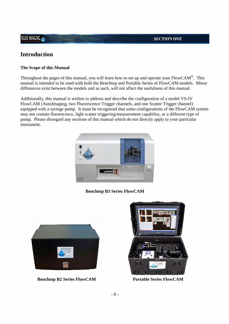
Introduction The Scope of this Manual Throughout the pages of this manual, you will learn how to set up and operate your FlowCAM®. This manual is intended to be used with both the Benchtop and Portable Series of FlowCAM models. Minor differences exist between the models and as such, will not affect the usefulness of this manual.

Additionally, this manual is written to address and describe the configuration of a model VS-IV FlowCAM (AutoImaging, two Fluorescence Trigger channels, and one Scatter Trigger channel) equipped with a syringe pump. It must be recognized that some configurations of the FlowCAM system may not contain fluorescence, light scatter triggering/measurement capability, or a different type of pump. Please disregard any sections of this manual which do not directly apply to your particular instrument.

Benchtop B3 Series FlowCAM

Benchtop B2 Series FlowCAM Portable Series FlowCAM

- 9 -

The FlowCAM® The FlowCAM® is an integrated system for rapidly analyzing particles in a moving fluid. The instrument combines selective capabilities of flow cytometry, microscopy, and fluorescence detection. The FlowCAM automatically counts, images, and analyzes the particles or cells in a sample or a continuous flow. Best of all, a FlowCAM can be customized to accommodate almost any environment or application. Originally developed for oceanographic investigations of organisms and particles in seawater, the FlowCAM provides the user with the capability to rapidly evaluate particulate matter in fluids. The instrument and software provides the user with tools to quickly and efficiently meet challenges that previously required multiple instruments and many hours of tedious work to complete. Your FlowCAM has the following features and capabilities:

· High-Speed Digital Imaging

· Particle Size, Count, and Shape

· Real-Time Bulk and Individual Particle Analysis

· The Combined Benefits of Multiple Instruments

· Compact and Durable Packaging

· Ability to Image Particles 2 µm to 3 mm in Diameter

· Fluorescence Detection Providing Additional Selectivity

· Scatter Detection for Low Particle Concentrations

Basic Overview of the FlowCAM In the FlowCAM system, sample is drawn into the flow chamber by a pump. Using the laser in Trigger Mode, the photomultiplier tubes (PMTs) and scatter detector monitor the fluorescence and light scatter of the passing particles. When a particle passing through the laser fan has sufficient fluorescence or laser light scatter, the camera is triggered to take an image of the field of view. The fluorescence value(s) and/or scatter detection value are then saved by VisualSpreadsheet (in addition to all other particle properties). The computer, digital signal processor, and trigger circuitry work together to initiate, retrieve and process images of the field of view. Groups of pixels that represent particles are then “segmented” out of each raw image and saved as a separate collage image (along with all associated parameter measurements). The process described above is similar when using AutoImage Mode, except the camera is set to capture raw images at a user defined interval.

- 10 -

Advanced Overview of the FlowCAM The FlowCAM architecture can be divided into three distinct systems:

· Optics · Fluidics · Electronics

Optics

Figure 1 is a block diagram of the FlowCAM architecture. The following section explains the operation of the components illustrated when using laser dependent Fluorescence and/or Scatter Trigger modes. As the particles are drawn into the flow chamber they pass through a “laser fan” that has been generated by the laser and a lens. Fluorescence which results from this illumination is passed back through the objective and the partial mirror. This light then passes through a system of optical filters and mirrors. The shorter wavelengths of green to orange are reflected by a mirror to the 500-600 nm fluorescence detector. Longer wavelength light passes

through another filter to the 600-700 nm fluorescence detector. Finally, a scatter detector is located at the end of the optical path (in the same cube as the flash LED) to detect any disturbances in the laser light. If either the fluorescence or scatter detector receives a strong enough signal, indicating the presence of a particle of interest, the flash LED is turned on for a very short interval. This light is then imaged with the objective onto the camera. A patented depth of focus enhancer stretches out the focus of the objective, thus enhancing the resolution of particle images. Fluidics

Sample fluid is drawn through the Flow chamber for analysis by a syringe pump and then deposited into an outflow collection. FlowCAM’s unique flow chamber is a key component to this system. Unlike conventional flow cytometers, the FlowCAM does not use a sheath fluid for hydrodynamic focusing (laminar flow). Instead, it uses a flow chamber with a variable size cross section. A complete list of the standard flow cell dimensions recommended for each objective is available in Appendix I. The appropriate flow chamber size is chosen by considering the following

interdependent factors:

· Objective Magnification · Size and Size Range of Particles Under Study · Desired Flow Rate · Viscosity of the Fluid

- 11 -

While the optimum values for each of these factors for a given application is usually determined through application development, a “starting point” is easily determined merely by looking at the particle size range under study. Electronics

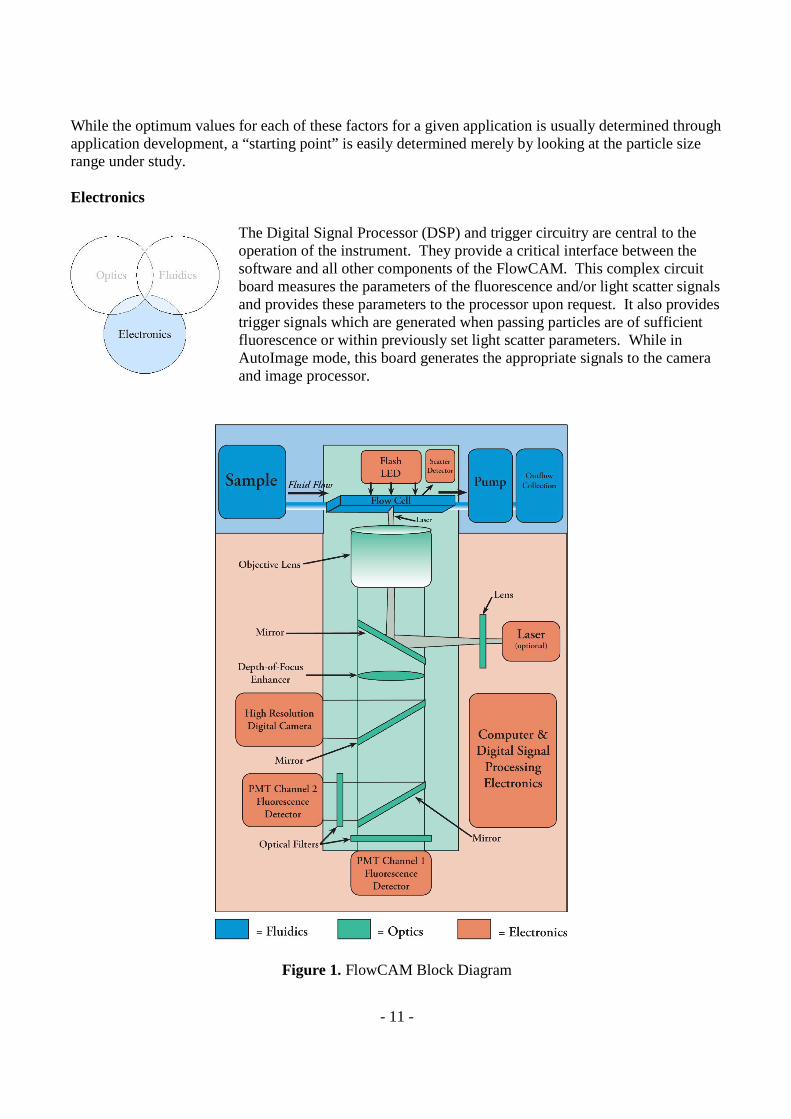
The Digital Signal Processor (DSP) and trigger circuitry are central to the operation of the instrument. They provide a critical interface between the software and all other components of the FlowCAM. This complex circuit board measures the parameters of the fluorescence and/or light scatter signals and provides these parameters to the processor upon request. It also provides trigger signals which are generated when passing particles are of sufficient fluorescence or within previously set light scatter parameters. While in AutoImage mode, this board generates the appropriate signals to the camera and image processor.

Figure 1. FlowCAM Block Diagram

- 12 -

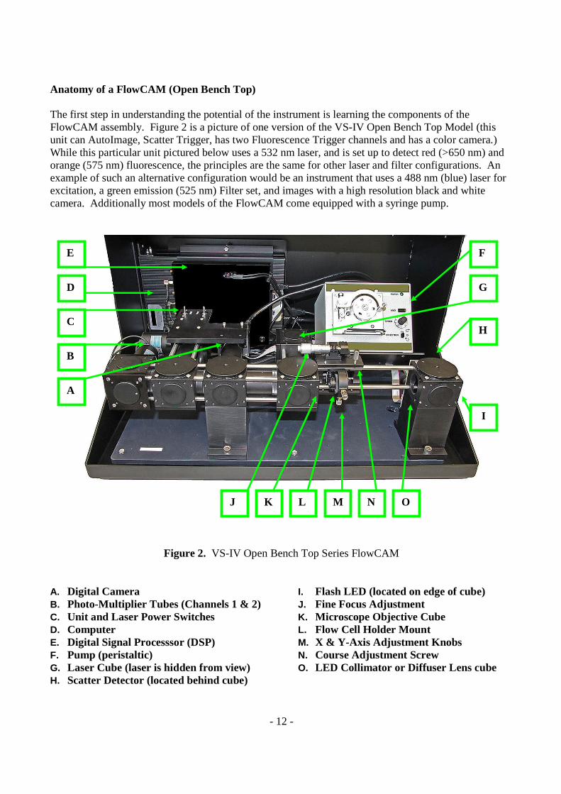
Anatomy of a FlowCAM (Open Bench Top)

The first step in understanding the potential of the instrument is learning the components of the FlowCAM assembly. Figure 2 is a picture of one version of the VS-IV Open Bench Top Model (this unit can AutoImage, Scatter Trigger, has two Fluorescence Trigger channels and has a color camera.) While this particular unit pictured below uses a 532 nm laser, and is set up to detect red (>650 nm) and orange (575 nm) fluorescence, the principles are the same for other laser and filter configurations. An example of such an alternative configuration would be an instrument that uses a 488 nm (blue) laser for excitation, a green emission (525 nm) Filter set, and images with a high resolution black and white camera. Additionally most models of the FlowCAM come equipped with a syringe pump.

Figure 2. VS-IV Open Bench Top Series FlowCAM

A. Digital Camera B. Photo-Multiplier Tubes (Channels 1 & 2) C. Unit and Laser Power Switches D. Computer E. Digital Signal Processsor (DSP) F. Pump (peristaltic) G. Laser Cube (laser is hidden from view) H. Scatter Detector (located behind cube)

I. Flash LED (located on edge of cube) J. Fine Focus Adjustment K. Microscope Objective Cube L. Flow Cell Holder Mount M. X & Y-Axis Adjustment Knobs N. Course Adjustment Screw O. LED Collimator or Diffuser Lens cube

D

E

A

F

C

B

I

J K M N O

G

H

L

- 13 -

Modes of Operation - AutoImage Mode & Trigger Mode Understanding AutoImage Mode (Including File Reprocessing Mode)

· AutoImage Mode defined · Particle Concentration Calculation: AutoImage Mode · Setup & Focus (Camera Image Preview) · AutoImage Mode (No Save) · AutoImage Mode · File Processing Mode (No Save) · File Processing Mode

Understanding Trigger Mode (Fluorescence & Scatter)

· Trigger Mode defined · Particle Concentration Calculation: Trigger Mode · Trigger Mode Setup · Trigger Mode (No Save) · Trigger Mode: Fluorescence (Channels 1 & 2) and Laser Light Scatter · Important Information Regarding Trigger Mode

Understanding AutoImage Mode AutoImage Mode Definition AutoImage Mode is an image analysis mode in which the FlowCAM captures images of the moving fluid at a regular, user-defined interval (Frames Per Second or FPS). This mode is used when processing samples with high particle concentrations. The total number of particles imaged is a function of the following:

· concentration and properties of particles in the sample fluid · camera field of view (FOV) dimensions · total number of field of view images (taken at a regular, user-defined interval) that were analyzed

The volume analyzed is determined based on flow cell dimensions and the concentration of particles is reported at the end of the run. In other words, the concentration of particles in the sample fluid is determined by dividing the total number of particles imaged (counted) by the total volume of sample fluid imaged. The concentration is automatically calculated using the following information:

- 14 -

· total number of particles imaged (counted) · field of view dimensions (based on a calibration factor for microns/pixel) · depth and width of the flow cell · total number of frames that were collected

Fluid Volume for AutoImage Mode The value for Fluid Volume Imaged for AutoImage mode is automatically generated at the end of a run using the method shown below under Particle Concentration Calculation. The value for “Fluid Volume Imaged” corresponds to the actual number of milliliters that were imaged for that particular AutoImage analysis. Particle Concentration Calculation: AutoImage Mode A summary of the following calculation description can be found in Appendix III. For AutoImage Mode analysis, the method to determine particle concentration of an unconstrained camera field is as described in the following paragraph. There are several values that are measured by VisualSpreadsheet that are required for the calculation of Particle Concentration (P/mL or PPM):

· Particle Count · Area Based Diameter (ABD) of each particle · Equivalent Spherical Diameter (ESD) of each particle · Total number of camera images taken for the full duration of the analysis

There are also several parameters that are user defined that VisualSpreadsheet uses in the calculation:

· Acceptable range of camera view · Flow cell depth (D) in µm

The acceptable range of camera view is dependent on the properties of the digital camera. Depending on the model of the digital camera, the maximum and minimum number of pixels may be different than the values used below in the example calculations. Typical values for camera pixels are 1024 x 768 and 1280 x 960. The FlowCAM will arrive with factory default settings that include the correct values for the installed digital camera. VisualSpreadsheet determines the acceptable region within the camera’s field of view by the following process. Note that the acceptable range of the camera can be changed or “constrained” by the user: Left = user-specified number (default value = 0 pixels) Right = user-specified number (default value = 1279 pixels) Top = user-specified number (default value = 0 pixels) Bottom = user-specified number (default value = 959 pixels) With these numbers specified, VisualSpreadsheet can then determine the height and width of the acceptable region with the following calculations:

- 15 -

Height (H) = (1 + (Bottom - Top)) x the Calibration Factor (µm per pixel)

Width (W) = (1 + (Right - Left)) x the Calibration Factor (µm per pixel) Depth (D) = User defined value determined by the dimensions of the flow cell used during the analysis

Note: The Calibration Factor (used for H and W) is factory determined and the value set as a default value.

The Volume per Picture is calculated as D × H × W (µm3) VisualSpreadsheet can determine the total volume it imaged with the following calculation: Total Volume Imaged = Number of Images Taken during the Run × Volume per Picture (µm3)

VisualSpreadsheet can calculate PPM using either the ESD or ABD measurements. Total Volume of Particles using ESD or ABD (µm3) PPM = ————————————————————— X 106 Total Volume Imaged (µm3) Particle Count 1 x 1012 (µm3) P/mL = ———————————— X ——————— Total Volume Imaged (µm3) 1 (mL) To locate the values used in the above calculations, from the Main window:

· For Height and Width, Setup > Context > Capture (tab) > Acceptable Region (section), to view the total number of pixels from left to right, and from top to bottom.

· For Depth, Setup > Context > Flow Cell (tab) > Flow cell (section) for the “Flow cell depth” value (populated from the Flow Cell Database file).

· For total number of camera images, Setup > Context > Run Summary (tab) > Images > Total. Setup and Focus (Camera Image Preview) The Setup and Focus window (Setup Menu or Hotkey = F6) is used to adjust the focus, camera, and context settings of the FlowCAM while sample is present in a flowcell. By default, in AutoImage Mode, the camera images the field of view at a regular interval-determined by the AutoImage Rate setting in frames per second (Setup > Context > Camera > Timing [section]). The resulting images are displayed in the Setup and Focus window. This window can be used for centering the flow cell, or for “real time” particle monitoring. Note that Raw camera images shown in the Setup and Focus window are neither captured nor saved with the following exception: before exiting Setup & Focus mode or while paused, the last image in the viewer can be saved (this is described in more detail in Section Four).

- 16 -

AutoImage Mode (No Save) In AutoImage Mode (No Save) (Setup Menu or Hotkey = F7), the user can view how the software will segment the field of view raw images into the collage window. This No Save mode is an excellent tool to test the effects of using different context settings and to make a final adjustment of the focus. This Mode is described in more detail in Section Four. AutoImage Mode In AutoImage Mode (Setup Menu or Hotkey = F4), the particles in the field of view are imaged and captured at a regular interval. The operator uses the pulldown menu “Analyze” and selects AutoImage Mode. Images of all captured particles and their Particle Properties are stored on the hard drive along with Summary Statistics and Calculated Values (Calculated Values include statistical information such as Mean, Standard Deviation, etc.). File Processing Mode (No Save) File Processing Mode (No Save) (Setup Menu) is used to process raw images captured to disk during a previous sample run. VisualSpreadsheet has the ability to save Raw Camera Images while running an AutoImage or Trigger Mode analysis. If the user has selected the option to save raw camera images, File Processing Mode can be used at a later time to reprocess these raw images. Reprocessing of these previously collected raw images can be useful for testing the efficiency of capturing particles of interest under different context settings. Therefore, this mode can assist the user in optimizing how particles are captured without actually running additional sample through the unit. The results of this Mode are not saved. This Mode is described in more detail in Section Four. File Processing Mode File Processing Mode (Analyze Menu) is used to process raw images captured to the hard drive during a previous sample run. This mode functions exactly as File Processing Mode (No Save) except that the results of this Mode are saved.

Understanding Trigger Mode (Fluorescence & Scatter) Trigger Mode Definition Trigger Mode is an image analysis mode on the FlowCAM in which the scattering of laser light is measured and/or two photo multiplier tubes (PMT) are used to measure fluorescent particles, and those measurements are compared against a threshold value. When a particle passes through the laser and generates a signal that meets or exceeds one of the threshold values, the camera is triggered to take an image. Camera triggering is thus based upon the Threshold value. Each particle currently in the objective’s field of view will be captured in this image. Once this raw image is captured, VisualSpreadsheet will then apply the context settings you have previously entered to this image and process the raw image.

- 17 -

The user should use Trigger Mode when the sample contains fluorescent particles or organisms and you want to capture only these specific particles. Additionally, use Trigger Mode if you have a very dilute sample and you wish to ensure that you capture an image of the entire particle, rather than risk capturing only a partial image (which can occur in AutoImage Mode). Particle Concentration Calculation: Trigger Mode For additional information regarding this calculation, please refer to the section “Particle Concentration Calculation: AutoImage Mode”. In Trigger Mode, the concentration of particles in the sample fluid imaged is a function of:

· number and properties of particles in the sample fluid · width of the field of view · width of the flow cell · total volume of sample fluid that passed through the flow cell

The software will calculate the actual number of milliliters that passed through the field of view. For Trigger Mode runs, the value for Fluid Volume is the total number of millilitres that passed through the instrument. Trigger Mode Setup In Trigger Mode Setup (F8) (Setup Menu or Hotkey = F8), the user can view the rate of triggering. This is similar to the Setup and Focus Mode described above, however, a camera image of the field of view is captured only when the predetermined fluorescence or light scatter threshold is exceeded by a particle. Note that before exiting this mode or while paused, the image in the viewer can be saved (this will be described in detail in Section Four). Trigger Mode (No Save) In Trigger Mode (No Save) (Setup Menu or Hotkey = F9), the user can view the rate of triggering and observe how the software will segment the field of view image into the collage window. This Mode is a good tool to use to test the effects of using different context settings and to make a final adjustment of the focus. Trigger Mode: Fluorescence (Channels 1 & 2) and Laser Light Scatter For this mode, the user chooses “Trigger Mode” from the pull down Analyze menu (Hotkey = F5). When triggering on fluorescence, the field of view is imaged when the intensity of fluorescence of passing particles exceeds a user set threshold. When triggering on light scatter, the field of view is imaged when the intensity of the light scatter signal exceeds a user set threshold. Measured values are then saved with the images (along with all other relevant statistics and particle properties). Important Information Regarding Trigger Mode As you attempt to optimize an analysis done in Trigger Mode, it is important to note that there are a few factors that may affect the performance of your FlowCAM in Trigger Mode.

- 18 -

When using a FlowCAM, your objective lens does not view the entire width of the flow cell. If you are using the FlowCAM for counting purposes, you might want to consider using a field-of-view (FOV) flow cell - this will allow you to image the entire fluid stream. The FOV flow cells are available for purchase from Fluid Imaging Technologies, Inc. If you are not suspending your sample in a dense or viscous fluid, or you are not occasionally stirring the sample in the funnel, you may get a settling effect. You may notice that as the fluid level in your funnel decreases, particles may stick to the side of the funnel. If you see this settling effect you will want to carefully mix the funnel contents. During an analysis you can also open the Time Series Graph (you can view this graph in “real time” as you are running your sample). To open this graph: select Tools > Time Series Graph. The user can display several different plots including a “Frequency Plot” (by right clicking on the graph). If the sample is settling, you should notice a gradual decrease in the slope of the trend line. This decrease indicates that your sample could be slowly settling out of solution. It is possible to capture images of particles that did not trigger the laser or the PMT. This happens because once the threshold level is met or exceeded, the camera takes a raw image, and VisualSpreadsheet will capture all particle(s) based on your context settings. If there is more than one particle in the raw image, VisualSpreadsheet has no way to determine which particle produced the trigger signal. Therefore the PMT/Scatter data values are assigned to all particles within that raw image. To avoid this situation, the user should dilute the sample to a concentration where the software is only capturing one particle per used image. To assist the user with determining if the test sample is too concentrated for optimal Trigger Mode analysis, VisualSpreadsheet calculates a Particles Per Used Image value. The user can open a “Particles Per Used Image” value display in the capture window. While in the Setup and Focus [F6] capture window, select Show > Configure Display > and check the “show particles per used image” box. This number should ideally be between an average value of 1.00 and 1.10 (with 1.00 being the most optimal result). If your particles per used image value is larger than 1.10 you should continue to dilute your sample. Note that VisualSpreadsheet can account for this dilution of the sample solution. To enter the correct values for the dilution navigate to Setup > Context > Fluidics > Sample Dilution > and enable “The sample fluid was diluted or concentrated” > enter the correct ratio. The rate at which you set your pump can also influence both the image quality and number of particles you will collect. If the pump speed is too fast, you may find that the particle that caused the triggering event is already out of the objective’s field of view before the camera can take an image. This means that you may have zero particles being captured in your raw images. Slowing down the pump speed can help alleviate this problem. Remember that flow rate is a function of pump speed, pump tubing diameter, pump tubing elasticity, sample viscosity, and flow cell dimensions. The most effective way to determine the flow rate for a particular configuration is to measure the time required to pull a known volume of sample through a fully primed system. Post-analysis, users can open a .lst file from a previous run and correct the flow cell dimensions, fluid volume, etc. At this point, the data may be saved as another .lst file under a different name. This process is typically done if values have been entered incorrectly or additional sample was added to the funnel during the run, etc.

- 19 -

Instrument Setup

· Initial Setup and Instrument Configuration

· Optimizing the Field of View and Focus

· Maintenance and Shutting Down

Initial Setup and Instrument Configuration

Note that a basic “Quick Start” procedure (Appendix VI) and a list of standard Hardware configurations (Appendix VII) can be found at the end of this manual.

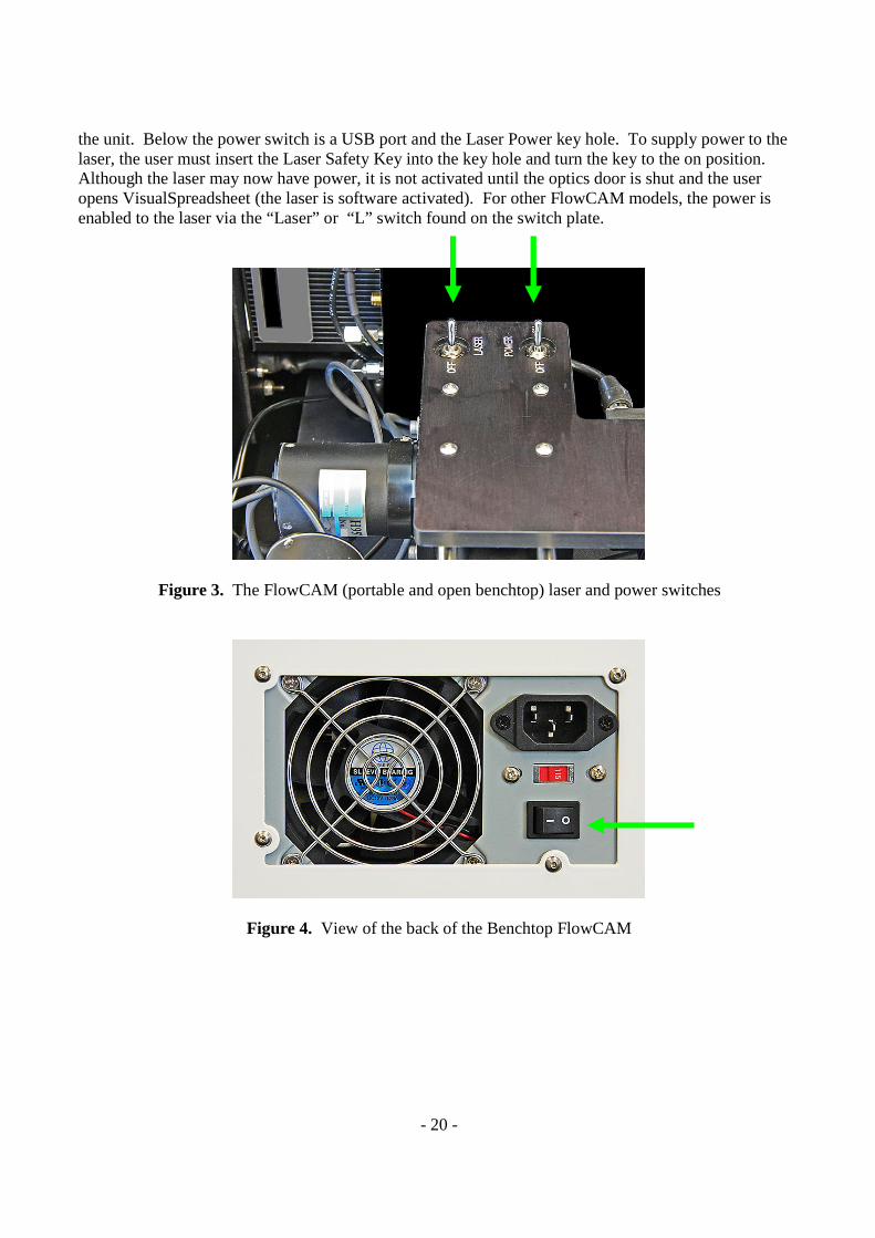
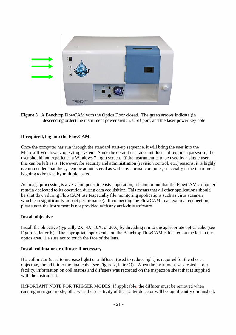
Power Configuration for a Portable FlowCAM Due to the portable nature of this model of the FlowCAM, it includes a power cord that will plug into a 12V power supply (for example, a power outlet in a vehicle). There are up to three other power cords for the Portable FlowCAM. These include a standard wall outlet cord and a cord for the wireless mouse charger. If your FlowCAM came with a USB hub, that may have be the third power cord. The Wireless Mouse and Keyboard Charger included with the FlowCAM can only be used in a 120V/60Hz power receptacle. Power Configuration for an Open Benchtop and Benchtop FlowCAM There are two power cords for the Benchtop FlowCAM. These two cords belong the FlowCAM and FlowCAM LCD Monitor. The monitor is usually powered up first. If the system is configured with a wireless mouse, it should be fully charged and the wireless keyboard must have batteries installed. The USB style mouse and keyboard draw power through the computer’s USB port. For the Benchtop FlowCAM, USB ports are located on the back of the instrument case. These ports are for connection of the Keyboard (USB), Mouse (USB), Monitor, and Network cable. Extra USB ports can also be found on the back (and one on the front) of this model of FlowCAM. Activate Power to the FlowCAM Locate and activate the power toggle marked “Power” or “P” on the switch plate. The switch plate location is illustrated in Figure 3 for an Open Benchtop and Portable FlowCAM. The power switch for a Benchtop FlowCAM is illustrated in Figure 4 and 5. On the back of the Benchtop FlowCAM (Figure 4), the Master power switch must first be switched to the On (I) position. The red 115 V switch can be toggled to 230 V to match the power supply of your country/location. On the front of the Benchtop FlowCAM (Figure 5), the Standard power switch must be switched to the On (I) position to power on

- 20 -

the unit. Below the power switch is a USB port and the Laser Power key hole. To supply power to the laser, the user must insert the Laser Safety Key into the key hole and turn the key to the on position. Although the laser may now have power, it is not activated until the optics door is shut and the user opens VisualSpreadsheet (the laser is software activated). For other FlowCAM models, the power is enabled to the laser via the “Laser” or “L” switch found on the switch plate.

Figure 3. The FlowCAM (portable and open benchtop) laser and power switches

Figure 4. View of the back of the Benchtop FlowCAM

- 21 -

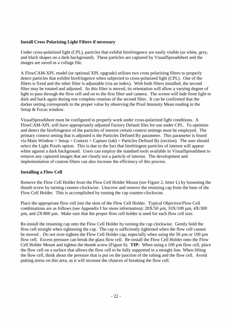
Figure 5. A Benchtop FlowCAM with the Optics Door closed. The green arrows indicate (in

descending order) the instrument power switch, USB port, and the laser power key hole If required, log into the FlowCAM Once the computer has run through the standard start-up sequence, it will bring the user into the Microsoft Windows 7 operating system. Since the default user account does not require a password, the user should not experience a Windows 7 login screen. If the instrument is to be used by a single user, this can be left as is. However, for security and administration (revision control, etc.) reasons, it is highly recommended that the system be administered as with any normal computer, especially if the instrument is going to be used by multiple users. As image processing is a very computer-intensive operation, it is important that the FlowCAM computer remain dedicated to its operation during data acquisition. This means that all other applications should be shut down during FlowCAM use (especially file monitoring applications such as virus scanners which can significantly impact performance). If connecting the FlowCAM to an external connection, please note the instrument is not provided with any anti-virus software. Install objective Install the objective (typically 2X, 4X, 10X, or 20X) by threading it into the appropriate optics cube (see Figure 2, letter K). The appropriate optics cube on the Benchtop FlowCAM is located on the left in the optics area. Be sure not to touch the face of the lens. Install collimator or diffuser if necessary If a collimator (used to increase light) or a diffuser (used to reduce light) is required for the chosen objective, thread it into the final cube (see Figure 2, letter O). When the instrument was tested at our facility, information on collimators and diffusers was recorded on the inspection sheet that is supplied with the instrument. IMPORTANT NOTE FOR TRIGGER MODES: If applicable, the diffuser must be removed when running in trigger mode, otherwise the sensitivity of the scatter detector will be significantly diminished.

- 22 -

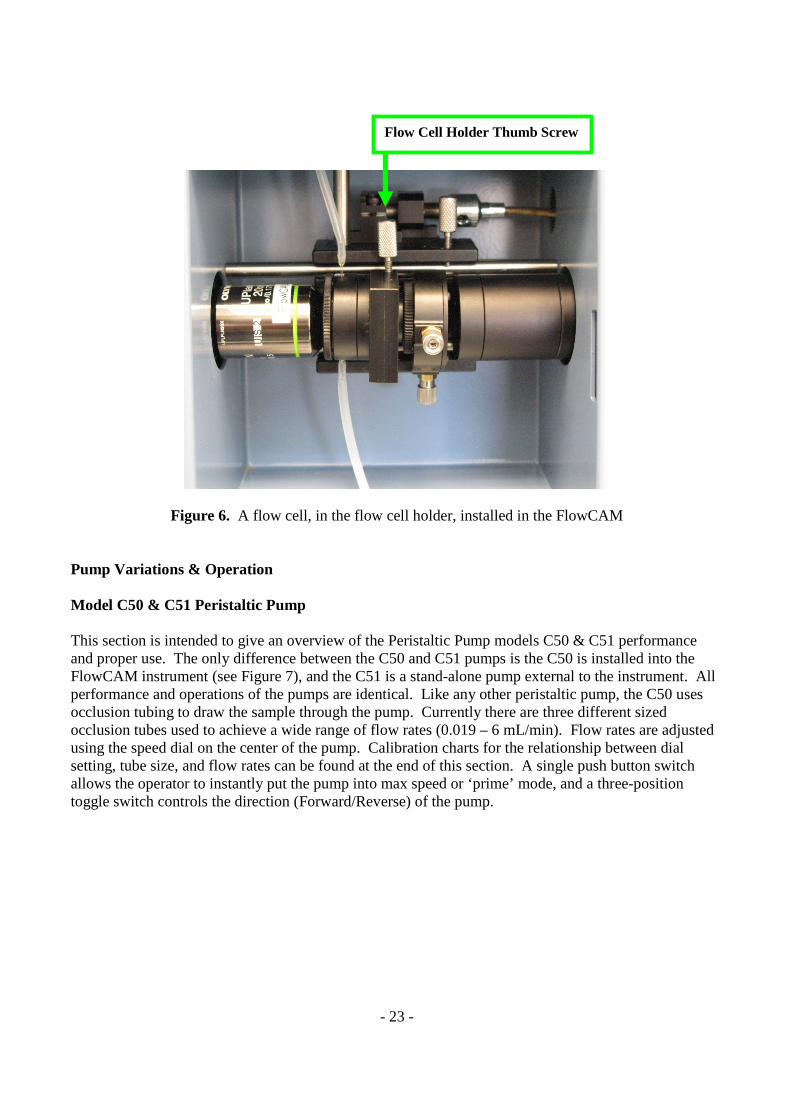
Install Cross Polarizing Light Filters if necessary Under cross-polarized light (CPL), particles that exhibit birefringence are easily visible (as white, grey, and black shapes on a dark background). These particles are captured by VisualSpreadsheet and the images are saved as a collage file. A FlowCAM-XPL model (or optional XPL upgrade) utilizes two cross polarizing filters to properly detect particles that exhibit birefringence when subjected to cross-polarized light (CPL). One of the filters is fixed and the other filter is adjustable (via an index). With both filters installed, the second filter may be rotated and adjusted. As this filter is moved, its orientation will allow a varying degree of light to pass through the flow cell and on to the first filter and camera. The screen will fade from light to dark and back again during one complete rotation of the second filter. It can be confirmed that the darker setting corresponds to the proper value by observing the Pixel Intensity Mean reading in the Setup & Focus window. VisualSpreadsheet must be configured to properly work under cross-polarized light conditions. A FlowCAM-XPL will have appropriately adjusted Factory Default files for use under CPL. To optimize and detect the birefringence of the particles of interest certain context settings must be employed. The primary context setting that is adjusted is the Particles Defined By parameter. This parameter is found via Main Window > Setup > Context > Capture (tab) > Particles Defined By (section). The user should select the Light Pixels option. This is due to the fact that birefringent particles of interest will appear white against a dark background. Users can employ the standard tools available in VisualSpreadsheet to remove any captured images that are clearly not a particle of interest. The development and implementation of custom filters can also increase the efficiency of this process. Installing a Flow Cell Remove the Flow Cell Holder from the Flow Cell Holder Mount (see Figure 2, letter L) by loosening the thumb screw by turning counter-clockwise. Unscrew and remove the retaining cap from the base of the Flow Cell Holder. This is accomplished by turning the cap counter-clockwise. Place the appropriate flow cell into the slots of the Flow Cell Holder. Typical Objective/Flow Cell combinations are as follows (see Appendix I for more information): 20X/50 µm, 10X/100 µm, 4X/300 µm, and 2X/800 µm. Make sure that the proper flow cell holder is used for each flow cell size. Re-install the retaining cap onto the Flow Cell Holder by turning the cap clockwise. Gently hold the flow cell straight when tightening the cap. The cap is sufficiently tightened when the flow cell cannot be moved . Do not over-tighten the Flow Cell Holder cap, especially when using the 50 µm or 100 µm flow cell. Excess pressure can break the glass flow cell. Re-install the Flow Cell Holder onto the Flow Cell Holder Mount and tighten the thumb screw (Figure 6). TIP: When using a 100 µm flow cell, place the flow cell on a surface that allows the flow cell to be fully supported in a straight line. When lifting the flow cell, think about the pressure that is put on the junction of the tubing and the flow cell. Avoid putting stress on this area, as it will increase the chances of breaking the flow cell.

- 23 -

Figure 6. A flow cell, in the flow cell holder, installed in the FlowCAM

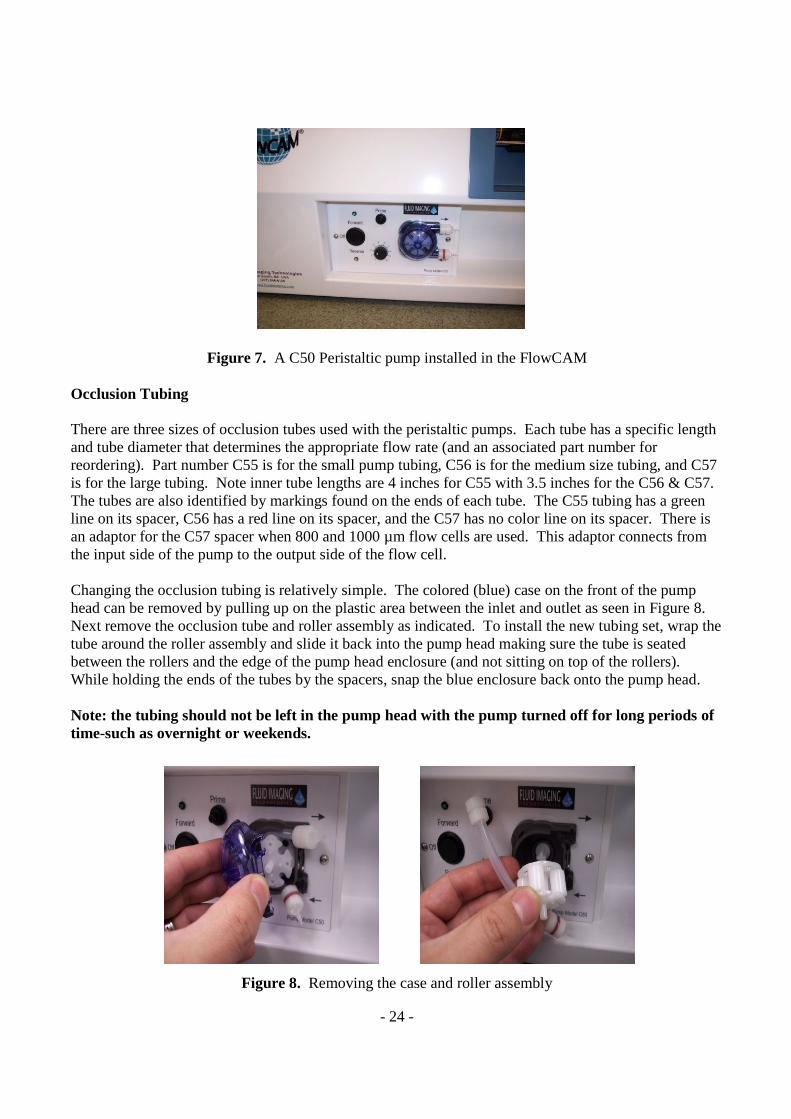
Pump Variations & Operation Model C50 & C51 Peristaltic Pump This section is intended to give an overview of the Peristaltic Pump models C50 & C51 performance and proper use. The only difference between the C50 and C51 pumps is the C50 is installed into the FlowCAM instrument (see Figure 7), and the C51 is a stand-alone pump external to the instrument. All performance and operations of the pumps are identical. Like any other peristaltic pump, the C50 uses occlusion tubing to draw the sample through the pump. Currently there are three different sized occlusion tubes used to achieve a wide range of flow rates (0.019 – 6 mL/min). Flow rates are adjusted using the speed dial on the center of the pump. Calibration charts for the relationship between dial setting, tube size, and flow rates can be found at the end of this section. A single push button switch allows the operator to instantly put the pump into max speed or ‘prime’ mode, and a three-position toggle switch controls the direction (Forward/Reverse) of the pump.

Flow Cell Holder Thumb Screw

- 24 -

Figure 7. A C50 Peristaltic pump installed in the FlowCAM Occlusion Tubing There are three sizes of occlusion tubes used with the peristaltic pumps. Each tube has a specific length and tube diameter that determines the appropriate flow rate (and an associated part number for reordering). Part number C55 is for the small pump tubing, C56 is for the medium size tubing, and C57 is for the large tubing. Note inner tube lengths are 4 inches for C55 with 3.5 inches for the C56 & C57. The tubes are also identified by markings found on the ends of each tube. The C55 tubing has a green line on its spacer, C56 has a red line on its spacer, and the C57 has no color line on its spacer. There is an adaptor for the C57 spacer when 800 and 1000 µm flow cells are used. This adaptor connects from the input side of the pump to the output side of the flow cell. Changing the occlusion tubing is relatively simple. The colored (blue) case on the front of the pump head can be removed by pulling up on the plastic area between the inlet and outlet as seen in Figure 8. Next remove the occlusion tube and roller assembly as indicated. To install the new tubing set, wrap the tube around the roller assembly and slide it back into the pump head making sure the tube is seated between the rollers and the edge of the pump head enclosure (and not sitting on top of the rollers). While holding the ends of the tubes by the spacers, snap the blue enclosure back onto the pump head. Note: the tubing should not be left in the pump head with the pump turned off for long periods of time-such as overnight or weekends.

Figure 8. Removing the case and roller assembly

- 25 -

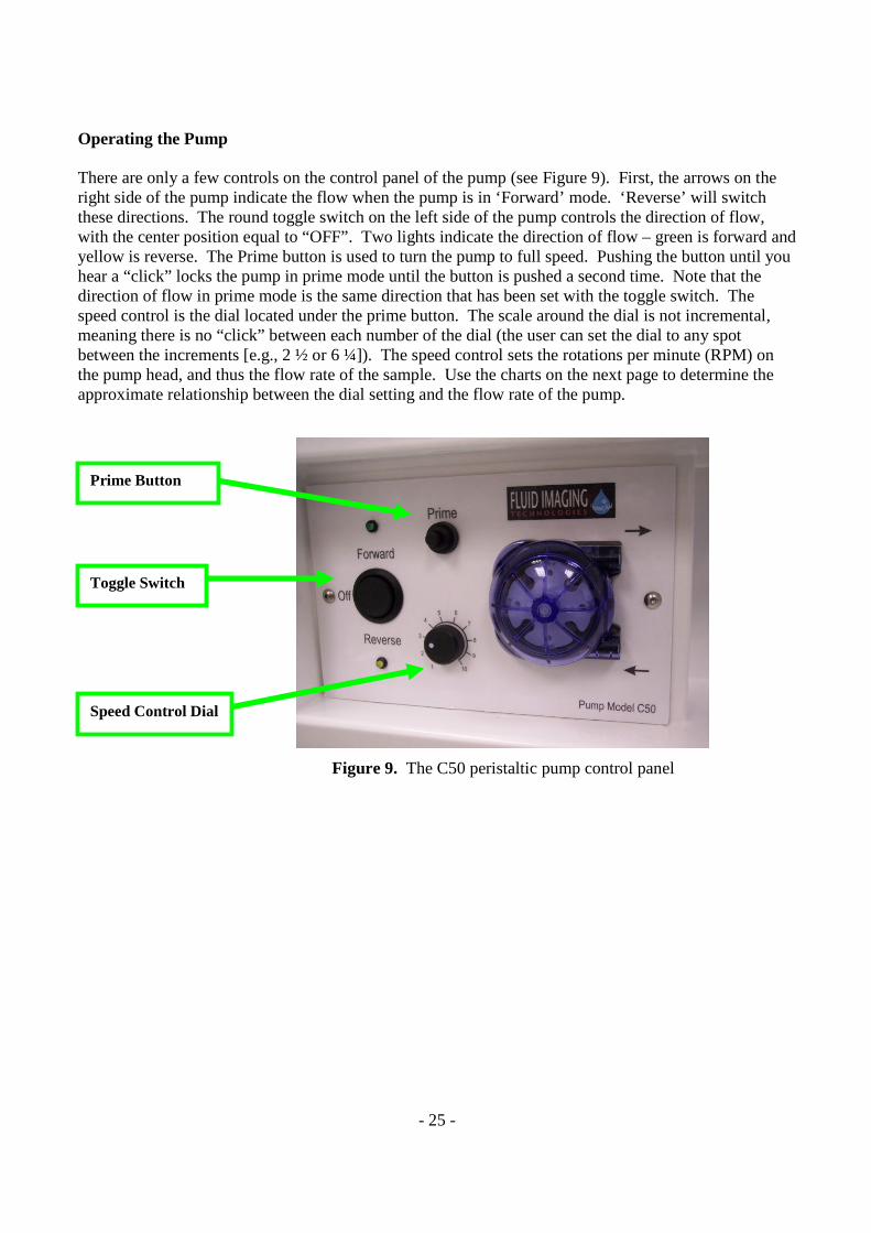
Operating the Pump There are only a few controls on the control panel of the pump (see Figure 9). First, the arrows on the right side of the pump indicate the flow when the pump is in ‘Forward’ mode. ‘Reverse’ will switch these directions. The round toggle switch on the left side of the pump controls the direction of flow, with the center position equal to “OFF”. Two lights indicate the direction of flow – green is forward and yellow is reverse. The Prime button is used to turn the pump to full speed. Pushing the button until you hear a “click” locks the pump in prime mode until the button is pushed a second time. Note that the direction of flow in prime mode is the same direction that has been set with the toggle switch. The speed control is the dial located under the prime button. The scale around the dial is not incremental, meaning there is no “click” between each number of the dial (the user can set the dial to any spot between the increments [e.g., 2 ½ or 6 ¼]). The speed control sets the rotations per minute (RPM) on the pump head, and thus the flow rate of the sample. Use the charts on the next page to determine the approximate relationship between the dial setting and the flow rate of the pump.

Figure 9. The C50 peristaltic pump control panel

Speed Control Dial

Toggle Switch

Prime Button

- 26 -

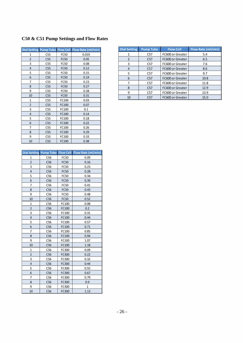
Dial Setting Pump Tube Flow Cell Flow Rate (ml/min)1 C55 FC50 0.0192 C55 FC50 0.053 C55 FC50 0.084 C55 FC50 0.125 C55 FC50 0.156 C55 FC50 0.197 C55 FC50 0.238 C55 FC50 0.279 C55 FC50 0.2810 C55 FC50 0.311 C55 FC100 0.032 C55 FC100 0.073 C55 FC100 0.14 C55 FC100 0.145 C55 FC100 0.186 C55 FC100 0.227 C55 FC100 0.268 C55 FC100 0.299 C55 FC100 0.3310 C55 FC100 0.38

Dial Setting Pump Tube Flow Cell Flow Rate (ml/min)1 C57 FC600 or Greater 5.42 C57 FC600 or Greater 6.53 C57 FC600 or Greater 7.64 C57 FC600 or Greater 8.65 C57 FC600 or Greater 9.76 C57 FC600 or Greater 10.87 C57 FC600 or Greater 11.88 C57 FC600 or Greater 12.99 C57 FC600 or Greater 13.910 C57 FC600 or Greater 15.0

Dial Setting Pump Tube Flow Cell Flow Rate (ml/min)1 C56 FC50 0.092 C56 FC50 0.163 C56 FC50 0.234 C56 FC50 0.285 C56 FC50 0.346 C56 FC50 0.397 C56 FC50 0.418 C56 FC50 0.439 C56 FC50 0.4810 C56 FC50 0.521 C56 FC100 0.082 C56 FC100 0.23 C56 FC100 0.314 C56 FC100 0.445 C56 FC100 0.576 C56 FC100 0.717 C56 FC100 0.858 C56 FC100 0.949 C56 FC100 1.0710 C56 FC100 1.181 C56 FC300 0.092 C56 FC300 0.223 C56 FC300 0.324 C56 FC300 0.445 C56 FC300 0.556 C56 FC300 0.677 C56 FC300 0.798 C56 FC300 0.99 C56 FC300 110 C56 FC300 1.13

C50 & C51 Pump Settings and Flow Rates

- 27 -

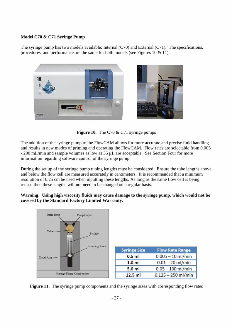
Model C70 & C71 Syringe Pump The syringe pump has two models available: Internal (C70) and External (C71). The specifications, procedures, and performance are the same for both models (see Figures 10 & 11).

Figure 10. The C70 & C71 syringe pumps

The addition of the syringe pump to the FlowCAM allows for more accurate and precise fluid handling and results in new modes of priming and operating the FlowCAM. Flow rates are selectable from 0.005 - 200 mL/min and sample volumes as low as 35 µL are acceptable. See Section Four for more information regarding software control of the syringe pump. During the set up of the syringe pump tubing lengths must be considered. Ensure the tube lengths above and below the flow cell are measured accurately in centimeters. It is recommended that a minimum resolution of 0.25 cm be used when inputting these lengths. As long as the same flow cell is being reused then these lengths will not need to be changed on a regular basis. Warning: Using high viscosity fluids may cause damage to the syringe pump, which would not be covered by the Standard Factory Limited Warranty.

Figure 11. The syringe pump components and the syringe sizes with corresponding flow rates

- 28 -

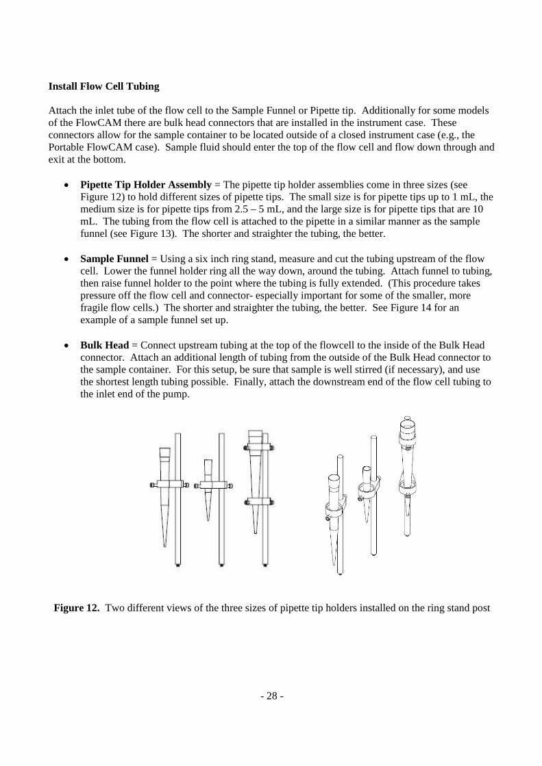
Install Flow Cell Tubing Attach the inlet tube of the flow cell to the Sample Funnel or Pipette tip. Additionally for some models of the FlowCAM there are bulk head connectors that are installed in the instrument case. These connectors allow for the sample container to be located outside of a closed instrument case (e.g., the Portable FlowCAM case). Sample fluid should enter the top of the flow cell and flow down through and exit at the bottom.

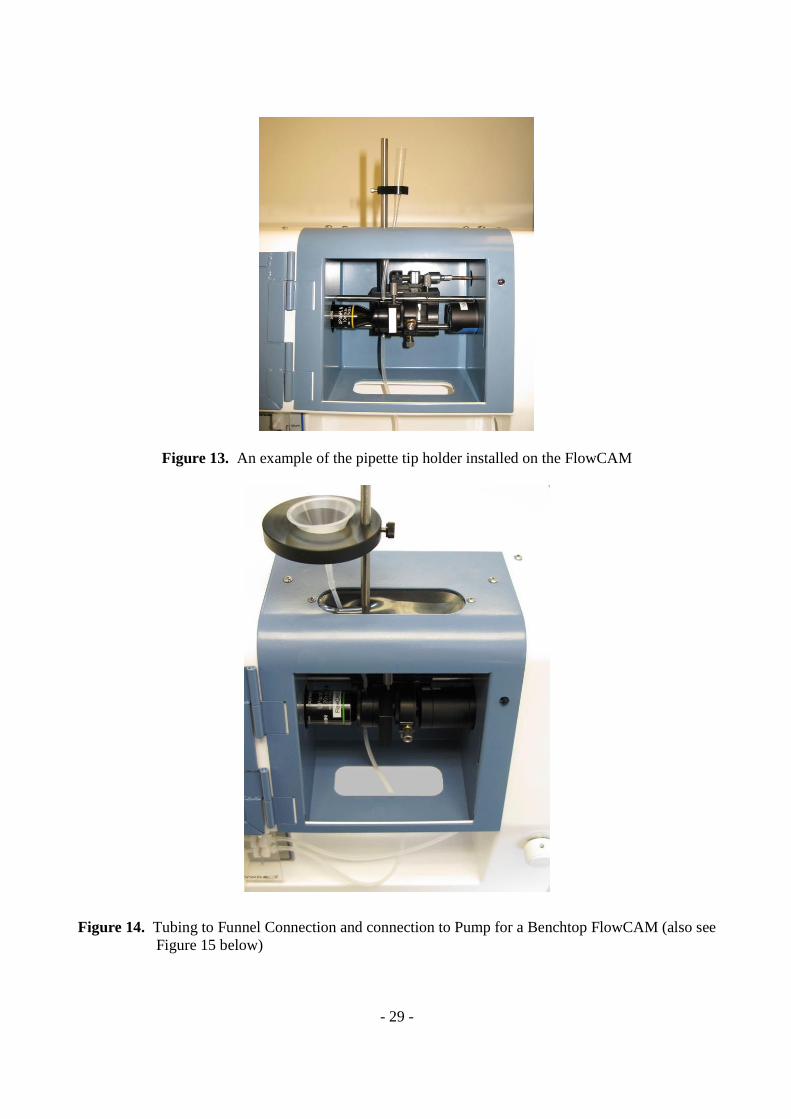
· Pipette Tip Holder Assembly = The pipette tip holder assemblies come in three sizes (see Figure 12) to hold different sizes of pipette tips. The small size is for pipette tips up to 1 mL, the medium size is for pipette tips from 2.5 – 5 mL, and the large size is for pipette tips that are 10 mL. The tubing from the flow cell is attached to the pipette in a similar manner as the sample funnel (see Figure 13). The shorter and straighter the tubing, the better.

· Sample Funnel = Using a six inch ring stand, measure and cut the tubing upstream of the flow

cell. Lower the funnel holder ring all the way down, around the tubing. Attach funnel to tubing, then raise funnel holder to the point where the tubing is fully extended. (This procedure takes pressure off the flow cell and connector- especially important for some of the smaller, more fragile flow cells.) The shorter and straighter the tubing, the better. See Figure 14 for an example of a sample funnel set up.

· Bulk Head = Connect upstream tubing at the top of the flowcell to the inside of the Bulk Head

connector. Attach an additional length of tubing from the outside of the Bulk Head connector to the sample container. For this setup, be sure that sample is well stirred (if necessary), and use the shortest length tubing possible. Finally, attach the downstream end of the flow cell tubing to the inlet end of the pump.

Figure 12. Two different views of the three sizes of pipette tip holders installed on the ring stand post

- 29 -

Figure 13. An example of the pipette tip holder installed on the FlowCAM

Figure 14. Tubing to Funnel Connection and connection to Pump for a Benchtop FlowCAM (also see

Figure 15 below)

- 30 -

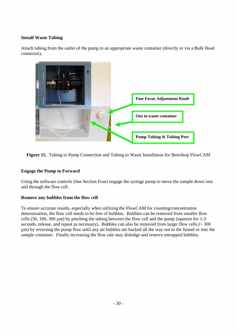
Install Waste Tubing Attach tubing from the outlet of the pump to an appropriate waste container (directly or via a Bulk Head connector).

Figure 15. Tubing to Pump Connection and Tubing to Waste Installation for Benchtop FlowCAM

Engage the Pump to Forward Using the software controls (See Section Four) engage the syringe pump to move the sample down into and through the flow cell. Remove any bubbles from the flow cell To ensure accurate results, especially when utilizing the FlowCAM for counting/concentration determination, the flow cell needs to be free of bubbles. Bubbles can be removed from smaller flow cells (50, 100, 300 µm) by pinching the tubing between the flow cell and the pump (squeeze for 1-3 seconds, release, and repeat as necessary). Bubbles can also be removed from larger flow cells (> 300 µm) by reversing the pump flow until any air bubbles are backed all the way out to the funnel or into the sample container. Finally increasing the flow rate may dislodge and remove entrapped bubbles.

Pump Tubing & Tubing Port

Fine Focus Adjustment Knob

Out to waste container

- 31 -

Optimizing the Field of View and Focus

Start the VisualSpreadsheet software by double-clicking on the icon located on the desktop. When prompted, select the appropriate magnification. A notification will open to remind the operator to ensure that the correct objective and collimator/diffuser (if required) is installed.

Figure 16. VisualSpreadsheet Icons

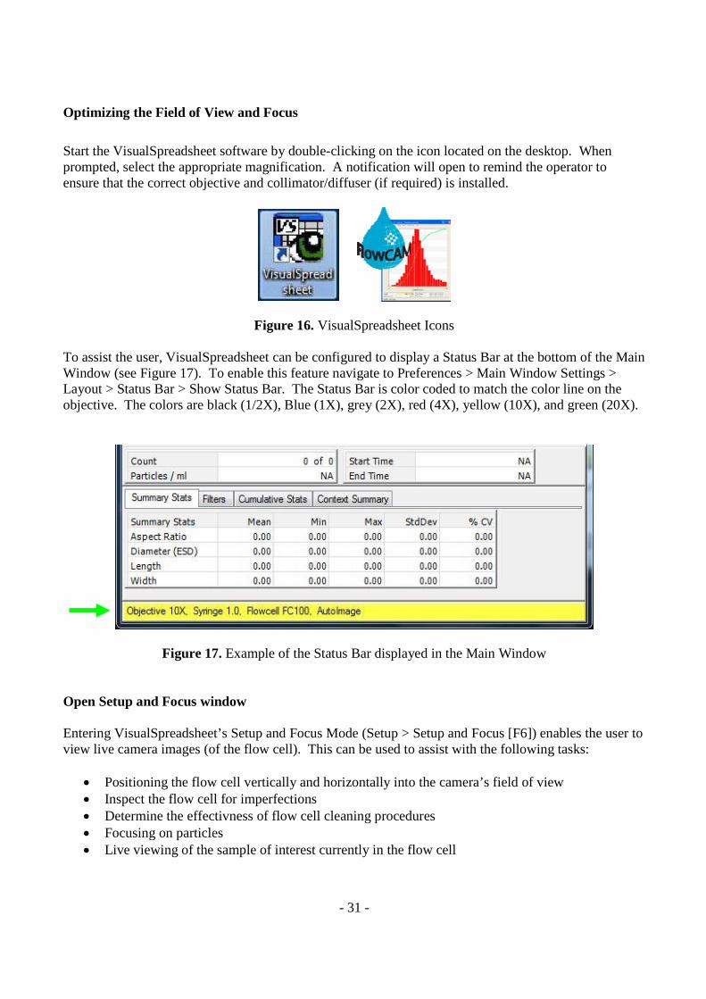
To assist the user, VisualSpreadsheet can be configured to display a Status Bar at the bottom of the Main Window (see Figure 17). To enable this feature navigate to Preferences > Main Window Settings > Layout > Status Bar > Show Status Bar. The Status Bar is color coded to match the color line on the objective. The colors are black (1/2X), Blue (1X), grey (2X), red (4X), yellow (10X), and green (20X).

Figure 17. Example of the Status Bar displayed in the Main Window Open Setup and Focus window Entering VisualSpreadsheet’s Setup and Focus Mode (Setup > Setup and Focus [F6]) enables the user to view live camera images (of the flow cell). This can be used to assist with the following tasks:

· Positioning the flow cell vertically and horizontally into the camera’s field of view · Inspect the flow cell for imperfections · Determine the effectivness of flow cell cleaning procedures · Focusing on particles · Live viewing of the sample of interest currently in the flow cell

- 32 -

Course/Rough focus To coarse focus the field of view, loosen the rail lock thumb screw (see Figure 18). Slide the entire Flow Cell Holder Assembly to bring any part of the flow cell into focus. When the flow cell has been located, tighten the rail lock thumb screw. WARNING: Extra care should be used with the 20X objective, to prevent it from coming in contact with (and potentially breaking) the 50 µm flow cell. Position adjustment of the flow cell Fine adjustments and positioning of the flow cell is possible by use of the X- and Y-axis positioning screws (Figures 18 & 19). This adjustment should be done, for example, to move a scratch in the glass wall of the Flow Cell to a position outside of the field of view. For fine vertical movement of the Flow Cell, turn the Y-positioning screw. For fine horizontal movement of the Flow Cell, turn the X-positioning thumb screw.

Figure 18. Course and Fine focus adjustment screw and knobs (also refer to Figure 2, letter M)

Course Focus Adjustment Screw

X-Axis Adjustment Knob

Y-Axis Adjustment Knob

- 33 -

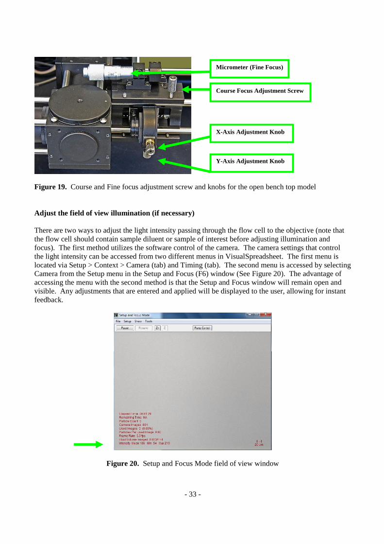
Figure 19. Course and Fine focus adjustment screw and knobs for the open bench top model Adjust the field of view illumination (if necessary) There are two ways to adjust the light intensity passing through the flow cell to the objective (note that the flow cell should contain sample diluent or sample of interest before adjusting illumination and focus). The first method utilizes the software control of the camera. The camera settings that control the light intensity can be accessed from two different menus in VisualSpreadsheet. The first menu is located via Setup > Context > Camera (tab) and Timing (tab). The second menu is accessed by selecting Camera from the Setup menu in the Setup and Focus (F6) window (See Figure 20). The advantage of accessing the menu with the second method is that the Setup and Focus window will remain open and visible. Any adjustments that are entered and applied will be displayed to the user, allowing for instant feedback.

Figure 20. Setup and Focus Mode field of view window

X-Axis Adjustment Knob

Y-Axis Adjustment Knob

Course Focus Adjustment Screw

Micrometer (Fine Focus)

- 34 -

The values for (Camera) Gain and Flash Duration can be adjusted to optimize the intensity of the field of view illumination.

· Adjust the Gain. The higher the value, the brighter the field of view. However, when this value is too high, there is a loss of contrast between particles and the background.

· Adjust the Flash Duration. Here again, the higher the value, the brighter the field of view. However, when this value is too high, images of the moving particles can begin to blur.

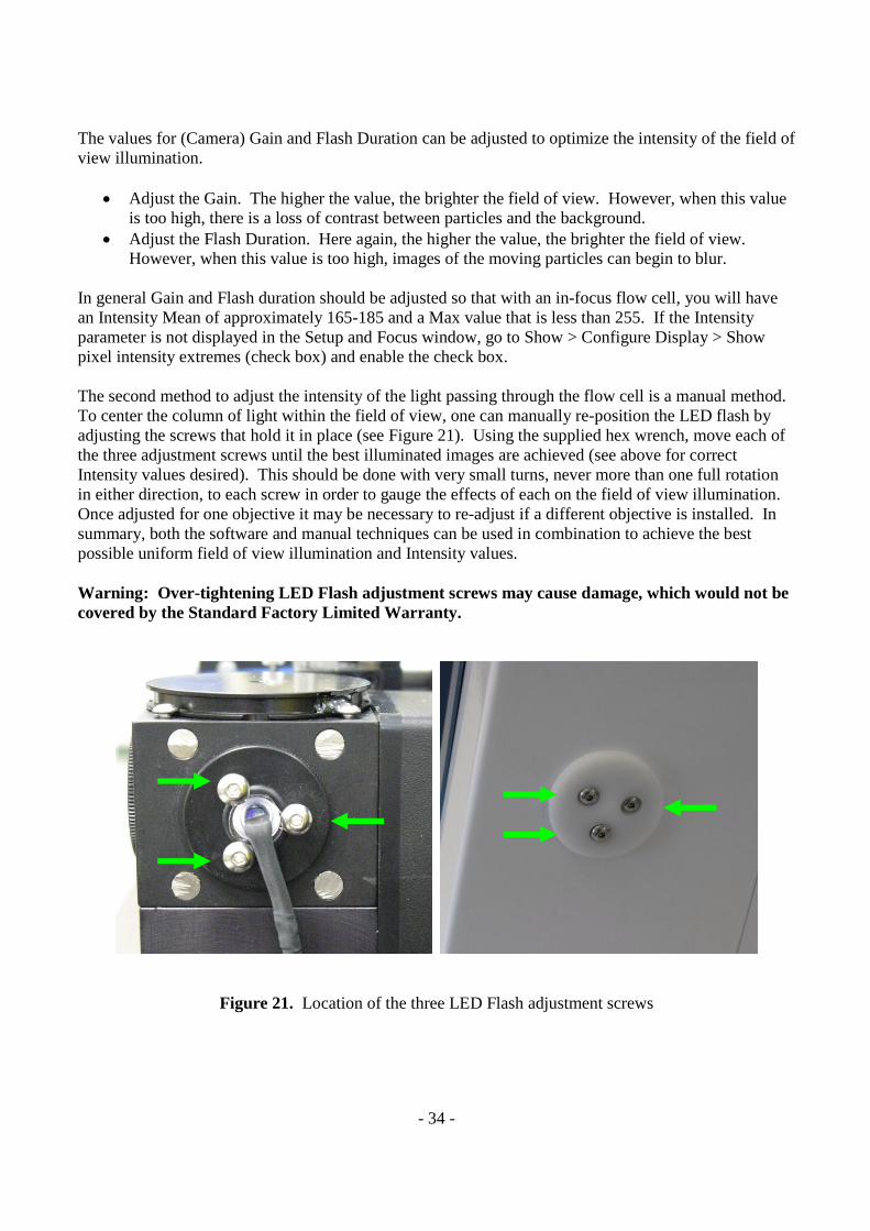
In general Gain and Flash duration should be adjusted so that with an in-focus flow cell, you will have an Intensity Mean of approximately 165-185 and a Max value that is less than 255. If the Intensity parameter is not displayed in the Setup and Focus window, go to Show > Configure Display > Show pixel intensity extremes (check box) and enable the check box. The second method to adjust the intensity of the light passing through the flow cell is a manual method. To center the column of light within the field of view, one can manually re-position the LED flash by adjusting the screws that hold it in place (see Figure 21). Using the supplied hex wrench, move each of the three adjustment screws until the best illuminated images are achieved (see above for correct Intensity values desired). This should be done with very small turns, never more than one full rotation in either direction, to each screw in order to gauge the effects of each on the field of view illumination. Once adjusted for one objective it may be necessary to re-adjust if a different objective is installed. In summary, both the software and manual techniques can be used in combination to achieve the best possible uniform field of view illumination and Intensity values. Warning: Over-tightening LED Flash adjustment screws may cause damage, which would not be covered by the Standard Factory Limited Warranty.

Figure 21. Location of the three LED Flash adjustment screws

- 35 -

Fine focus on Particles of Interest in the Sample Stop the pump (switch from “Forward” to “Off”, or “Pause” in Setup and Focus window when using the syringe pump) and use the Fine Focus Adjustment knob (Figure 15, Page 30) to bring particles of interest into focus (see Figure 19 for the location of the Micrometer Fine Focus Adjustment knob for the open Benchtop and Portable models). Another method to find the center of the flow cell and focus on that point is to locate the Fine Focus Adjustment knob position where one wall of the flow cell chamber is in focus. Next adjust the fine focus until the other wall of the chamber is in focus. Estimate and divide the difference between the two positions and center the plane of focus between the two walls at this estimated position. Alternatively, while observing the particles of interest in the sample fluid, the user can manipulate the micrometer (Figure 15 or 19) to manually bring these particles into focus. This method requires a minimum concentration of particles in the sample (to ensure particles are in the field of view) and the assumption that the particles are in the center of the flow cell. Now that the FlowCAM has been set up with the correct field of view illumination and particles of interest are in focus, you are ready to adjust context settings in Visual Spreadsheet and collect data. VisualSpreadsheet is described in detail in Section Four. When finished with data collection and image analysis, follow the Shut Down procedure described in the next section.

Shutting Down and Maintenance

Clean Flow Cell and Tubing Immediately after use, rinse the funnel and flow cell with deionized or distilled water. If necessary, precede this rinse with an appropriate solvent or surfactant in order to remove particles. This rinse will help keep the flow cells clear and free from contamination for day-to-day use. For longer storage periods, flow cells may be filled with a weak bleach solution (2 - 5%). The tubing can be sealed off on both ends to keep the solution from leaking out (or use a double ended tube connector to create a closed loop). Release Pump Tubing (Peristaltic Pumps Only) If using a peristaltic pump, to extend the life of pump tubing, release one end from the parastaltic rollers when the instrument is not in use. Once this section of tubing becomes worn and stretched, it can simply be replaced and discarded. Tip: Contact Fluid Imaging Technologies, Inc. for replacement tubing. Turn Off FlowCAM

· Turn off the laser (toggle off the “L” switch or use the laser safety key). · Close VisualSpreadsheet. Then go to the Start menu and select “Shut down”. The computer is

shut down once the screen goes completely blank. · Power off the monitor (the Portable FlowCAM will shut down the monitor automatically) and

the FlowCAM by switching off the “P” button (and the monitor power button if necessary).

- 36 -

General

· Keep the instrument as clean and dry as possible. · Store objectives and collimators either installed or in case/boxes provided.

o If there is no objective or collimator installed use removable tape or similar to cover the holes, thereby keeping dust and other miscellaneous particles out of the optics system.

· Never attempt to clean the mirrors located inside the FlowCAM. · Only clean objectives and collimators with an appropriate lens cloth or lens paper. · Never blow canned or compressed air into a FlowCAM. · Shut down the instrument when not in use. · Use caution with the fine focus knob to avoid over tightening or loosening. · Periodically check for inconsistent illumination in the viewing window.

o Use included hex key to adjust LED as necessary. · Do not unscrew the fine focus knob by traveling too far in either direction.

o Set to the center position periodically. · When required, a mixture of calibrated microspheres can be used to verify calibration (See

Appendix V).

Pumps Peristaltic (C50/51)

· When the pump is not in use unclip the occlusion tubing. This will extend the life of the tubing and provide the most consistent results.

o At the minimum, change the occlusion tubing every month. o If tubing looses elasticity (or displays indents) replace immediately.

· Perform a monthly check of pump performance by measuring the time needed to run 1 mL of water through an appropriate flow cell.

o Compare results to the flow ranges indicated on Page 27. · Never leave the pump running when away from the instrument. · Be aware of potential chemical reactions between the sample and the pump and flow cell tubing.

Note: Standard tubing is silicon based.

Syringe (C70/71)

· Check to make sure the syringe and bulkhead fittings are completely seated and there are no vacuum leaks at these junctions.

· Remove the bulkhead fittings on a regular basis and clean out any debris that may have accumulated. If any damage is incurred while the bulkhead fittings are being reseated, replacement parts are available from Fluid Imaging Technologies.

· Flush the pump with de-ionized water or appropriate cleaning solution daily. o Main window > Setup > Pump > Flush System

· Routinely take the syringe apart and clean the components.

- 37 -

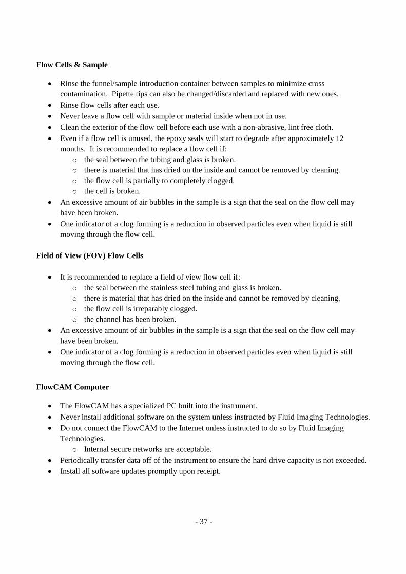
Flow Cells & Sample

· Rinse the funnel/sample introduction container between samples to minimize cross contamination. Pipette tips can also be changed/discarded and replaced with new ones.

· Rinse flow cells after each use. · Never leave a flow cell with sample or material inside when not in use. · Clean the exterior of the flow cell before each use with a non-abrasive, lint free cloth. · Even if a flow cell is unused, the epoxy seals will start to degrade after approximately 12

months. It is recommended to replace a flow cell if: o the seal between the tubing and glass is broken. o there is material that has dried on the inside and cannot be removed by cleaning. o the flow cell is partially to completely clogged. o the cell is broken.

· An excessive amount of air bubbles in the sample is a sign that the seal on the flow cell may have been broken.

· One indicator of a clog forming is a reduction in observed particles even when liquid is still moving through the flow cell.

Field of View (FOV) Flow Cells

· It is recommended to replace a field of view flow cell if: o the seal between the stainless steel tubing and glass is broken. o there is material that has dried on the inside and cannot be removed by cleaning. o the flow cell is irreparably clogged. o the channel has been broken.

· An excessive amount of air bubbles in the sample is a sign that the seal on the flow cell may have been broken.

· One indicator of a clog forming is a reduction in observed particles even when liquid is still moving through the flow cell.

FlowCAM Computer

· The FlowCAM has a specialized PC built into the instrument. · Never install additional software on the system unless instructed by Fluid Imaging Technologies. · Do not connect the FlowCAM to the Internet unless instructed to do so by Fluid Imaging

Technologies. o Internal secure networks are acceptable.

· Periodically transfer data off of the instrument to ensure the hard drive capacity is not exceeded. · Install all software updates promptly upon receipt.

- 38 -

VisualSpreadsheet

· Introduction to VisualSpreadsheet Run Files, Folders, and User Interface

· Main Window

· View Window

· Library Window

· Classification Window

Introduction to VisualSpreadsheet VisualSpreadsheet is the software program designed for the FlowCAM. It is indispensable for all the major aspects of analysis:

· Setup for data acquisition

· Data acquisition

· Post-processing of collected data

Run Files and Folders General Run File Name Information By default, the FlowCAM software generates filenames based on the Julian day of the experiment. The program stores data in files named as follows: JJJ-hhmmss.xxx where JJJ is the Julian day (1-365) and hhmmss represent the hours, minutes, and seconds for the start of the experiment. Finally .xxx is the filename extension for the stored file. The automatically generated default name for data files can be overridden. Whenever an experiment is conducted or a “Save As...” operation is performed, the user is prompted for the experiment name and the default is used only if an alternative is not entered. The FlowCAM software generates at least five files when an analysis is conducted. These files include a *.lst, *.ctx, *_notes.txt, *_run summary.txt, and *.tif files where the * is the common prefix the user selected to name this experiment or the JJJ-hhmmss name FlowCAM selects as a default. The software saves these files in the directory designated by the user.

- 39 -

When an analysis is started, VisualSpreadsheet prompts the user for an experiment name to use for the data files for this run. The program uses this name to prefix all of the data files for the run as well as to use as the folder name where the data files will be saved. VisualSpreadsheet stores the image data in non-compressed, lossless TIF file format with a *.tif file extension. These files are named with the common prefix and a number appended. So if the common prefix was 'my_experiment', then the image files would be named, my_experiment_000001.tif, my_experiment_000002.tif, etc.

Run Files

A “.lst” (list) file is generated for each experimental analysis. List files are the primary data files for FlowCAM experiments. List files are ASCII text files recording the fields of data collected for each particle. The format of this file has changed several times but the VisualSpreadsheet program can always read list files created by earlier versions of VisualSpreadsheet or older FlowCAM software. To extract the data in a list file for use with other software including spreadsheet programs like MS Excel, users can use the data Export functions in VisualSpreadsheet. All relevant data in a list file is made available using the Export functions. A context file with extension *.ctx is generated with each list file. It records the context information that was in effect when the list file was generated or when the experiment was run. The name of the context file uses the same common prefix as the other experiment files. The context file is a readable text file in the common Windows 'ini' file format. The context dialog box, accessed through the Setup > Context menu is used to modify the context settings. The “notes” text file accompanies the context file. The name follows the same convention, common prefix followed by _notes.txt. This file contains the experiment notes entered in the context dialog box. Folders User specific configuration and program behavior files are stored in a folder named VisualSpreadsheet in the user’s My Documents folder. The folders and .ini file found in the VisualSpreadsheet folder include:

· Class Templates: This is the folder where all class templates are stored by default. These templates allows a user to pull in a set of classes to populate with a new data set.

· Context: This is where manually saved context files are stored. · Default Context: This is where the context files that are “Saved as Local Default” are stored. · Filters: Default location to save newly created filters. · Layouts: Default location to save the Main window layout. · Logs: Default location for logs, generated when selected by going to Help > Advanced Tools >

Advanced Settings > Logging. · VisualSpreadsheet.ini file: Records and saves user preferences for window position, etc.

- 40 -

The Program Files for the Visual Spreadsheet program are by default located at C:\Program Files\VisualSpreadsheet. The items found at this location may include:

· Factory Defaults: This is where context settings, as determined by the factory, for this machine are stored. When the 'Load Factory Defaults' button is selected in the Context Load tab, you will be prompted to choose a context file from this directory.

· Firmware: Contains the firmware files required by the FlowCAM DSP board; this firmware is loaded by VisualSpreadsheet on first use.

· VisualSpreadsheet.exe: The VisualSpreadsheet program file. · Context Settings: This location is provided as a place to save custom context settings.

General Computer Specifications

The FlowCAM typically utilizes a Core 2 Duo, 2GB RAM and 500GB+ HD (larger hard drives are preferred for image storage). The Operating System presently used is Windows 7 but older systems employ Windows XP Pro. Overall, the typical new PC today should work with the VisualSpreadsheet satellite software package with a License dongle.

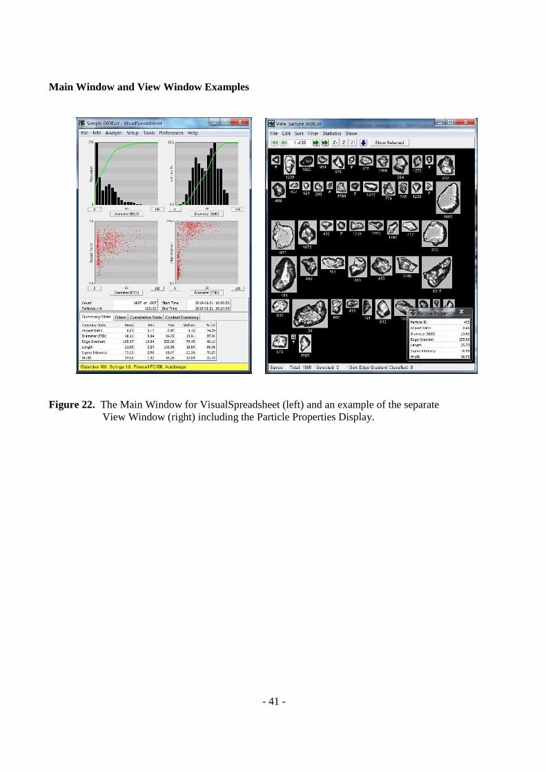
Overview of the VisualSpreadsheet User Interface It is important to begin by examining the overall user interface structure. Specific instructions and details are presented in the appropriate sections that follow. The VisualSpreadsheet Main Window (see Figure 22, left side window and Figure 23) is the primary control window for VisualSpreadsheet. In the Main window, you will find the primary menu commands for:

· Controlling the FlowCAM

· File Management

· Preferences

· Context Settings

Also contained within this window are two very important sub-elements; Interactive Graphs and Summary Statistics.

- 41 -

Main Window and View Window Examples

Figure 22. The Main Window for VisualSpreadsheet (left) and an example of the separate

View Window (right) including the Particle Properties Display.

- 42 -

Main Window

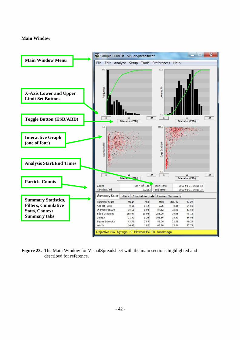
Figure 23. The Main Window for VisualSpreadsheet with the main sections highlighted and

described for reference.

Summary Statistics, Filters, Cumulative Stats, Context Summary tabs

Analysis Start/End Times

Particle Counts

Main Window Menu

Toggle Button (ESD/ABD)

X-Axis Lower and Upper Limit Set Buttons

Interactive Graph (one of four)

- 43 -

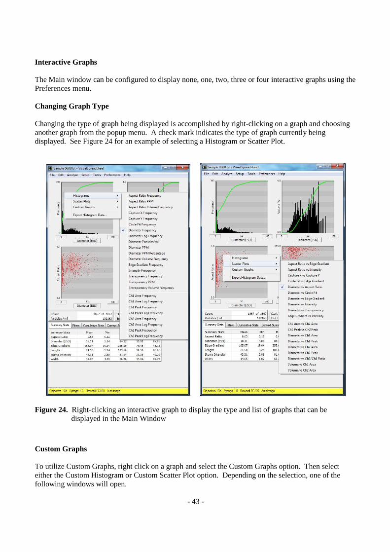
Interactive Graphs The Main window can be configured to display none, one, two, three or four interactive graphs using the Preferences menu. Changing Graph Type Changing the type of graph being displayed is accomplished by right-clicking on a graph and choosing another graph from the popup menu. A check mark indicates the type of graph currently being displayed. See Figure 24 for an example of selecting a Histogram or Scatter Plot.

Figure 24. Right-clicking an interactive graph to display the type and list of graphs that can be displayed in the Main Window

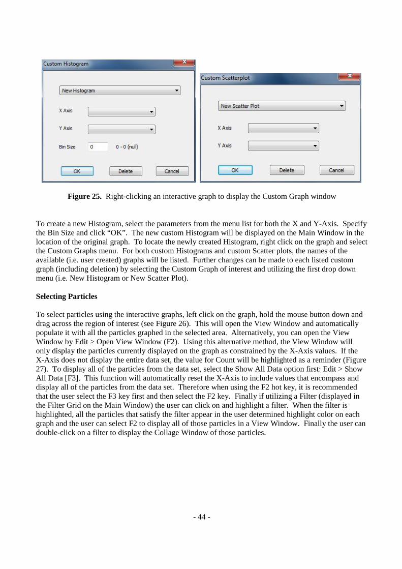
Custom Graphs To utilize Custom Graphs, right click on a graph and select the Custom Graphs option. Then select either the Custom Histogram or Custom Scatter Plot option. Depending on the selection, one of the following windows will open.

- 44 -

Figure 25. Right-clicking an interactive graph to display the Custom Graph window To create a new Histogram, select the parameters from the menu list for both the X and Y-Axis. Specify the Bin Size and click “OK”. The new custom Histogram will be displayed on the Main Window in the location of the original graph. To locate the newly created Histogram, right click on the graph and select the Custom Graphs menu. For both custom Histograms and custom Scatter plots, the names of the available (i.e. user created) graphs will be listed. Further changes can be made to each listed custom graph (including deletion) by selecting the Custom Graph of interest and utilizing the first drop down menu (i.e. New Histogram or New Scatter Plot). Selecting Particles To select particles using the interactive graphs, left click on the graph, hold the mouse button down and drag across the region of interest (see Figure 26). This will open the View Window and automatically populate it with all the particles graphed in the selected area. Alternatively, you can open the View Window by Edit > Open View Window (F2). Using this alternative method, the View Window will only display the particles currently displayed on the graph as constrained by the X-Axis values. If the X-Axis does not display the entire data set, the value for Count will be highlighted as a reminder (Figure 27). To display all of the particles from the data set, select the Show All Data option first: Edit > Show All Data [F3]. This function will automatically reset the X-Axis to include values that encompass and display all of the particles from the data set. Therefore when using the F2 hot key, it is recommended that the user select the F3 key first and then select the F2 key. Finally if utilizing a Filter (displayed in the Filter Grid on the Main Window) the user can click on and highlight a filter. When the filter is highlighted, all the particles that satisfy the filter appear in the user determined highlight color on each graph and the user can select F2 to display all of those particles in a View Window. Finally the user can double-click on a filter to display the Collage Window of those particles.

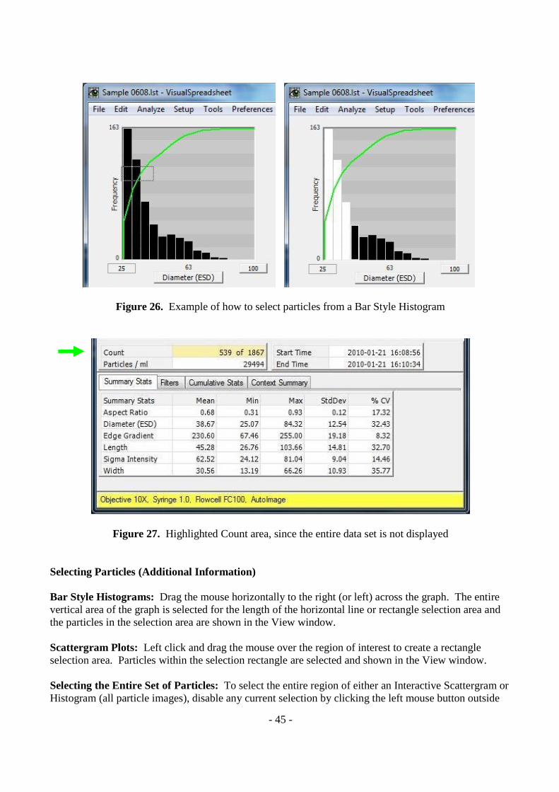
- 45 -

Figure 26. Example of how to select particles from a Bar Style Histogram

Figure 27. Highlighted Count area, since the entire data set is not displayed

Selecting Particles (Additional Information) Bar Style Histograms: Drag the mouse horizontally to the right (or left) across the graph. The entire vertical area of the graph is selected for the length of the horizontal line or rectangle selection area and the particles in the selection area are shown in the View window. Scattergram Plots: Left click and drag the mouse over the region of interest to create a rectangle selection area. Particles within the selection rectangle are selected and shown in the View window. Selecting the Entire Set of Particles: To select the entire region of either an Interactive Scattergram or Histogram (all particle images), disable any current selection by clicking the left mouse button outside

- 46 -

of any graph. Left click and drag the mouse over the entire graph area to create a rectangle selection area containing all particles. Again, particles selected are displayed in the View window. Selecting Particles without opening the View Window: To select particles without opening the View window, press and hold the Ctrl key down before dragging the cursor across or around the particles of interest in a graph. This is commonly done when particles are selected and then deleted using the Delete Selected Particles function (Edit > Delete Selected Particles) to eliminate particles that are not of interest. Main Window Data Grids and Summary Statistics

Several data grids selected by tabs are shown near the bottom of the Main Window. The selection of the grids that are included is made under Preferences > Main Window Settings > Grids. The Summary Statistics grid is configured via Preferences > Main Window Settings > Summary Statistics (tab). The user can select which calculated values (columns) and which Summary Statistics (rows) are displayed in this grid. The selected calculated values (Mean, Minimum, Maximum, Median, Standard Deviation, Coefficient of Variation, and D10/D25/D50(Median)/D75/D90) are listed for particles displayed in the Main window. Important note: The statistics displayed in the Summary Statistics grid are for “currently selected” particles only. For example when the interactive graph selection method is used, the particle statistics are updated to reflect only the particles selected within the graph. The data for all particles can be displayed by closing the View Window if open and left clicking on an area in the Main window outside any of the graphs (in the gray area). The following Figures (28-31) show examples of the various Main Window grids.

Figure 28. An example of the Summary Stats grid from the Main Window

Figure 29. An example of the Filters grid from the Main Window

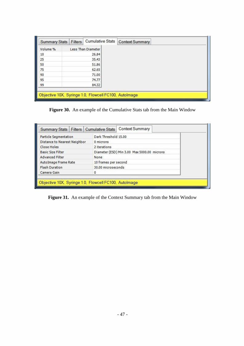
- 47 -

Figure 30. An example of the Cumulative Stats tab from the Main Window

Figure 31. An example of the Context Summary tab from the Main Window

- 48 -

Main Window

File Menu

The file menu is used to read and write (save) different file types. See additional information in this section for VisualSpreadsheet file types and detailed information on each kind of file. Open List… Use this function to open a previously generated FlowCAM list file. When Open List is selected, a file open dialog box will be displayed showing only List (.lst) files available in the current directory (usually the last directory opened). An example of a list file opened in the Main Window can be seen in Figure 23. If VisualSpreadsheet is directed to open a List file that was collected with a different magnification than the currently selected magnification, an error message will be displayed. For example, if the 4X version of VisualSpreadsheet is used to open a List file collected with 10X magnification, then the following error appears to alert the user. Note that when “OK” is selected, the List will open. However the Status Bar will still display the correct Objective and color for the currently selected magnification. Note: If opening list files from older versions of VisualSpreadsheet (2.4.1 or earlier) please see the section on “Recalculate”.

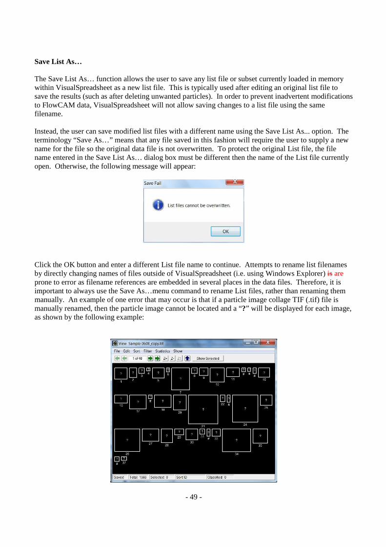
- 49 -

Save List As… The Save List As… function allows the user to save any list file or subset currently loaded in memory within VisualSpreadsheet as a new list file. This is typically used after editing an original list file to save the results (such as after deleting unwanted particles). In order to prevent inadvertent modifications to FlowCAM data, VisualSpreadsheet will not allow saving changes to a list file using the same filename. Instead, the user can save modified list files with a different name using the Save List As... option. The terminology “Save As…” means that any file saved in this fashion will require the user to supply a new name for the file so the original data file is not overwritten. To protect the original List file, the file name entered in the Save List As… dialog box must be different then the name of the List file currently open. Otherwise, the following message will appear:

Click the OK button and enter a different List file name to continue. Attempts to rename list filenames by directly changing names of files outside of VisualSpreadsheet (i.e. using Windows Explorer) is are prone to error as filename references are embedded in several places in the data files. Therefore, it is important to always use the Save As…menu command to rename List files, rather than renaming them manually. An example of one error that may occur is that if a particle image collage TIF (.tif) file is manually renamed, then the particle image cannot be located and a “?” will be displayed for each image, as shown by the following example:

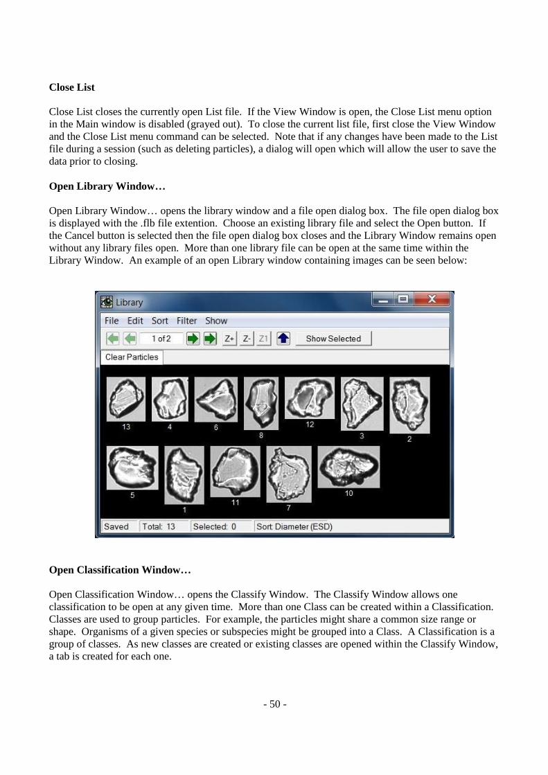
- 50 -

Close List Close List closes the currently open List file. If the View Window is open, the Close List menu option in the Main window is disabled (grayed out). To close the current list file, first close the View Window and the Close List menu command can be selected. Note that if any changes have been made to the List file during a session (such as deleting particles), a dialog will open which will allow the user to save the data prior to closing. Open Library Window… Open Library Window… opens the library window and a file open dialog box. The file open dialog box is displayed with the .flb file extention. Choose an existing library file and select the Open button. If the Cancel button is selected then the file open dialog box closes and the Library Window remains open without any library files open. More than one library file can be open at the same time within the Library Window. An example of an open Library window containing images can be seen below:

Open Classification Window… Open Classification Window… opens the Classify Window. The Classify Window allows one classification to be open at any given time. More than one Class can be created within a Classification. Classes are used to group particles. For example, the particles might share a common size range or shape. Organisms of a given species or subspecies might be grouped into a Class. A Classification is a group of classes. As new classes are created or existing classes are opened within the Classify Window, a tab is created for each one.

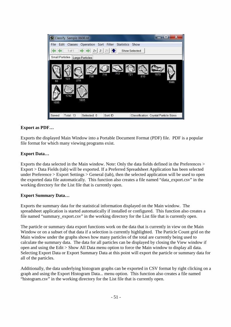
- 51 -

Export as PDF… Exports the displayed Main Window into a Portable Document Format (PDF) file. PDF is a popular file format for which many viewing programs exist. Export Data… Exports the data selected in the Main window. Note: Only the data fields defined in the Preferences > Export > Data Fields (tab) will be exported. If a Preferred Spreadsheet Application has been selected under Preference > Export Settings > General (tab), then the selected application will be used to open the exported data file automatically. This function also creates a file named “data_export.csv” in the working directory for the List file that is currently open. Export Summary Data… Exports the summary data for the statistical information displayed on the Main window. The spreadsheet application is started automatically if installed or configured. This function also creates a file named “summary_export.csv” in the working directory for the List file that is currently open. The particle or summary data export functions work on the data that is currently in view on the Main Window or on a subset of that data if a selection is currently highlighted. The Particle Count grid on the Main window under the graphs shows how many particles of the total are currently being used to calculate the summary data. The data for all particles can be displayed by closing the View window if open and using the Edit > Show All Data menu option to force the Main window to display all data. Selecting Export Data or Export Summary Data at this point will export the particle or summary data for all of the particles. Additionally, the data underlying histogram graphs can be exported in CSV format by right clicking on a graph and using the Export Histogram Data... menu option. This function also creates a file named “histogram.csv” in the working directory for the List file that is currently open.

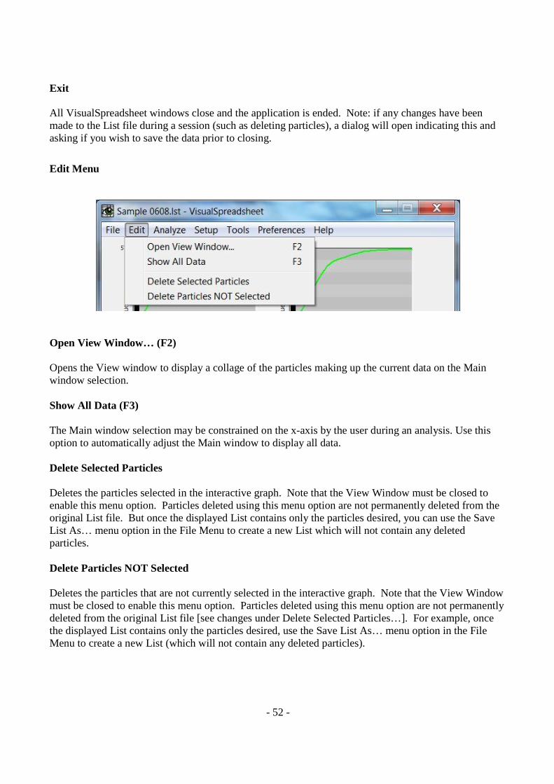
- 52 -

Exit All VisualSpreadsheet windows close and the application is ended. Note: if any changes have been made to the List file during a session (such as deleting particles), a dialog will open indicating this and asking if you wish to save the data prior to closing.

Edit Menu

Open View Window… (F2) Opens the View window to display a collage of the particles making up the current data on the Main window selection. Show All Data (F3) The Main window selection may be constrained on the x-axis by the user during an analysis. Use this option to automatically adjust the Main window to display all data. Delete Selected Particles Deletes the particles selected in the interactive graph. Note that the View Window must be closed to enable this menu option. Particles deleted using this menu option are not permanently deleted from the original List file. But once the displayed List contains only the particles desired, you can use the Save List As… menu option in the File Menu to create a new List which will not contain any deleted particles. Delete Particles NOT Selected Deletes the particles that are not currently selected in the interactive graph. Note that the View Window must be closed to enable this menu option. Particles deleted using this menu option are not permanently deleted from the original List file [see changes under Delete Selected Particles…]. For example, once the displayed List contains only the particles desired, use the Save List As… menu option in the File Menu to create a new List (which will not contain any deleted particles).

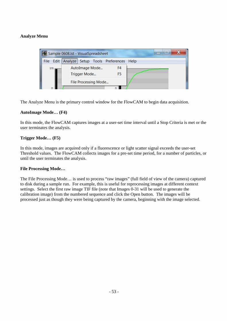
- 53 -

Analyze Menu

The Analyze Menu is the primary control window for the FlowCAM to begin data acquisition. AutoImage Mode… (F4) In this mode, the FlowCAM captures images at a user-set time interval until a Stop Criteria is met or the user terminates the analysis. Trigger Mode… (F5) In this mode, images are acquired only if a fluorescence or light scatter signal exceeds the user-set Threshold values. The FlowCAM collects images for a pre-set time period, for a number of particles, or until the user terminates the analysis. File Processing Mode… The File Processing Mode… is used to process “raw images” (full field of view of the camera) captured to disk during a sample run. For example, this is useful for reprocessing images at different context settings. Select the first raw image TIF file (note that Images 0-31 will be used to generate the calibration image) from the numbered sequence and click the Open button. The images will be processed just as though they were being captured by the camera, beginning with the image selected.

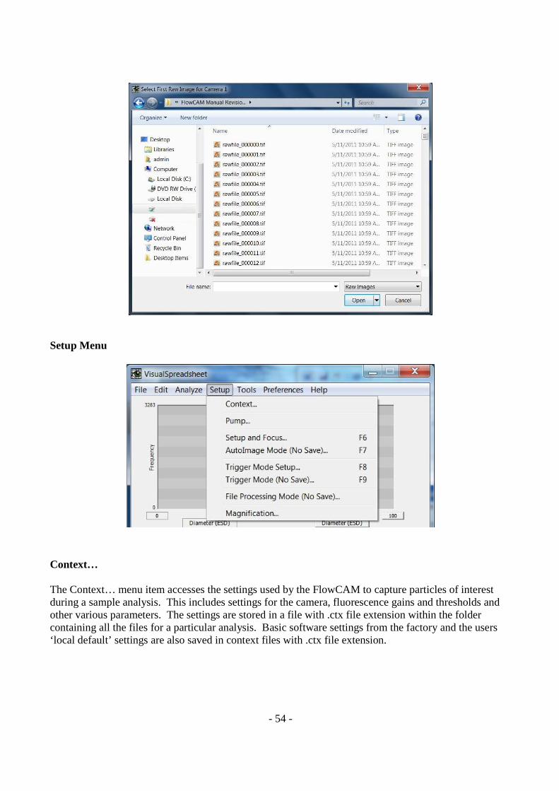
- 54 -

Setup Menu

Context… The Context… menu item accesses the settings used by the FlowCAM to capture particles of interest during a sample analysis. This includes settings for the camera, fluorescence gains and thresholds and other various parameters. The settings are stored in a file with .ctx file extension within the folder containing all the files for a particular analysis. Basic software settings from the factory and the users ‘local default’ settings are also saved in context files with .ctx file extension.

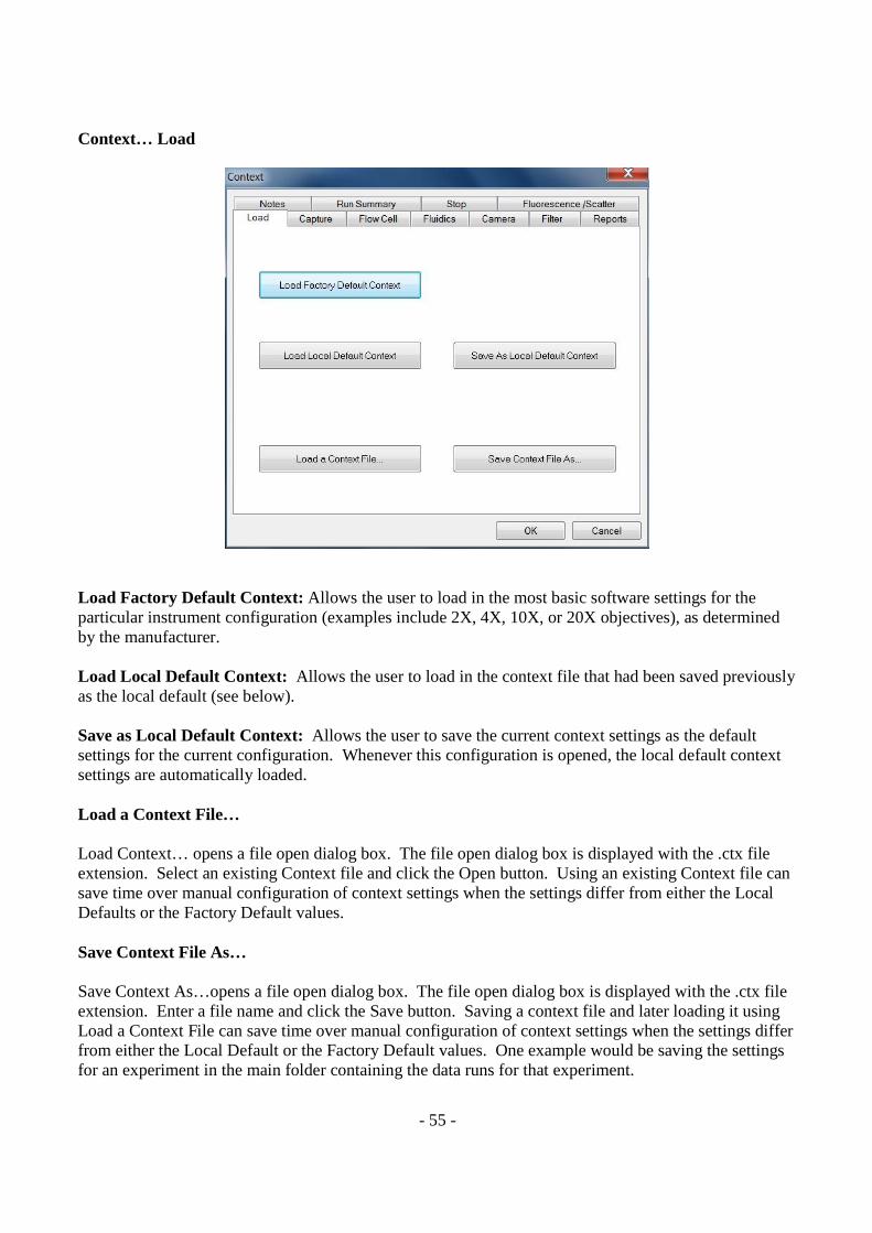
- 55 -

Context… Load

Load Factory Default Context: Allows the user to load in the most basic software settings for the particular instrument configuration (examples include 2X, 4X, 10X, or 20X objectives), as determined by the manufacturer. Load Local Default Context: Allows the user to load in the context file that had been saved previously as the local default (see below). Save as Local Default Context: Allows the user to save the current context settings as the default settings for the current configuration. Whenever this configuration is opened, the local default context settings are automatically loaded. Load a Context File… Load Context… opens a file open dialog box. The file open dialog box is displayed with the .ctx file extension. Select an existing Context file and click the Open button. Using an existing Context file can save time over manual configuration of context settings when the settings differ from either the Local Defaults or the Factory Default values. Save Context File As… Save Context As…opens a file open dialog box. The file open dialog box is displayed with the .ctx file extension. Enter a file name and click the Save button. Saving a context file and later loading it using Load a Context File can save time over manual configuration of context settings when the settings differ from either the Local Default or the Factory Default values. One example would be saving the settings for an experiment in the main folder containing the data runs for that experiment.

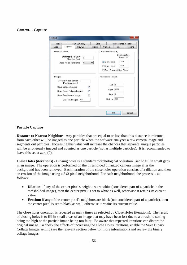
- 56 -

Context… Capture

Particle Capture Distance to Nearest Neighbor - Any particles that are equal to or less than this distance in microns from each other will be imaged as one particle when the software analyzes a raw camera image and segments out particles. Increasing this value will increase the chances that separate, unique particles will be erroneously imaged and counted as one particle (not as multiple particles). It is recommended to leave this set at zero (0). Close Holes (iterations) - Closing holes is a standard morphological operation used to fill in small gaps in an image. The operation is performed on the thresholded binarized camera image after the background has been removed. Each iteration of the close holes operation consists of a dilation and then an erosion of the image using a 3x3 pixel neighborhood. For each neighborhood, the process is as follows:

· Dilation: if any of the center pixel's neighbors are white (considered part of a particle in the thresholded image), then the center pixel is set to white as well, otherwise it retains its current value.

· Erosion: if any of the center pixel's neighbors are black (not considered part of a particle), then the center pixel is set to black as well, otherwise it retains its current value.

The close holes operation is repeated as many times as selected by Close Holes (iterations). The result of closing holes is to fill in small areas of an image that may have been lost due to a threshold setting being too high or the particle image being too faint. Be aware that repeated iterations can distort the original image. To check the effects of increasing the Close Holes iterations, enable the Save Binary Collage Images setting (see the relevant section below for more information) and review the binary collage images.

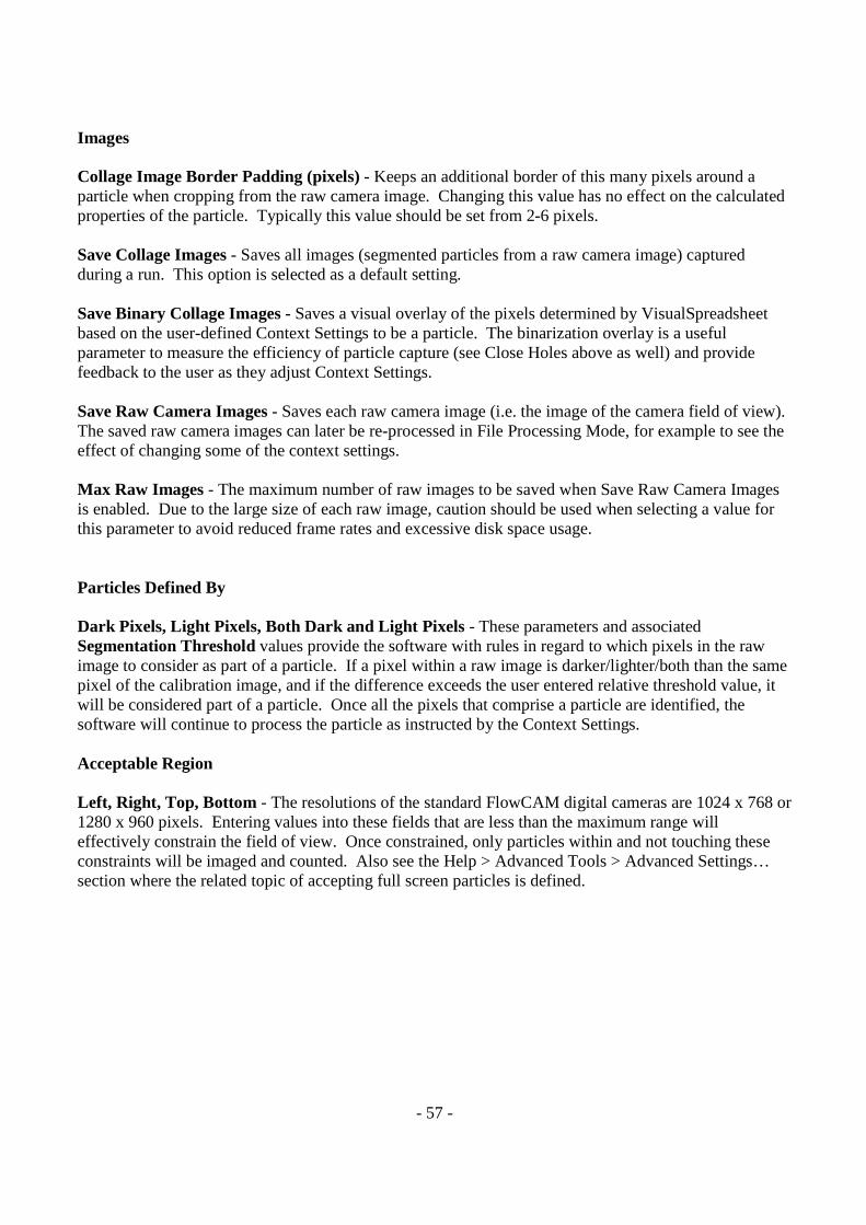
- 57 -

Images Collage Image Border Padding (pixels) - Keeps an additional border of this many pixels around a particle when cropping from the raw camera image. Changing this value has no effect on the calculated properties of the particle. Typically this value should be set from 2-6 pixels. Save Collage Images - Saves all images (segmented particles from a raw camera image) captured during a run. This option is selected as a default setting. Save Binary Collage Images - Saves a visual overlay of the pixels determined by VisualSpreadsheet based on the user-defined Context Settings to be a particle. The binarization overlay is a useful parameter to measure the efficiency of particle capture (see Close Holes above as well) and provide feedback to the user as they adjust Context Settings. Save Raw Camera Images - Saves each raw camera image (i.e. the image of the camera field of view). The saved raw camera images can later be re-processed in File Processing Mode, for example to see the effect of changing some of the context settings. Max Raw Images - The maximum number of raw images to be saved when Save Raw Camera Images is enabled. Due to the large size of each raw image, caution should be used when selecting a value for this parameter to avoid reduced frame rates and excessive disk space usage. Particles Defined By Dark Pixels, Light Pixels, Both Dark and Light Pixels - These parameters and associated Segmentation Threshold values provide the software with rules in regard to which pixels in the raw image to consider as part of a particle. If a pixel within a raw image is darker/lighter/both than the same pixel of the calibration image, and if the difference exceeds the user entered relative threshold value, it will be considered part of a particle. Once all the pixels that comprise a particle are identified, the software will continue to process the particle as instructed by the Context Settings. Acceptable Region Left, Right, Top, Bottom - The resolutions of the standard FlowCAM digital cameras are 1024 x 768 or 1280 x 960 pixels. Entering values into these fields that are less than the maximum range will effectively constrain the field of view. Once constrained, only particles within and not touching these constraints will be imaged and counted. Also see the Help > Advanced Tools > Advanced Settings… section where the related topic of accepting full screen particles is defined.

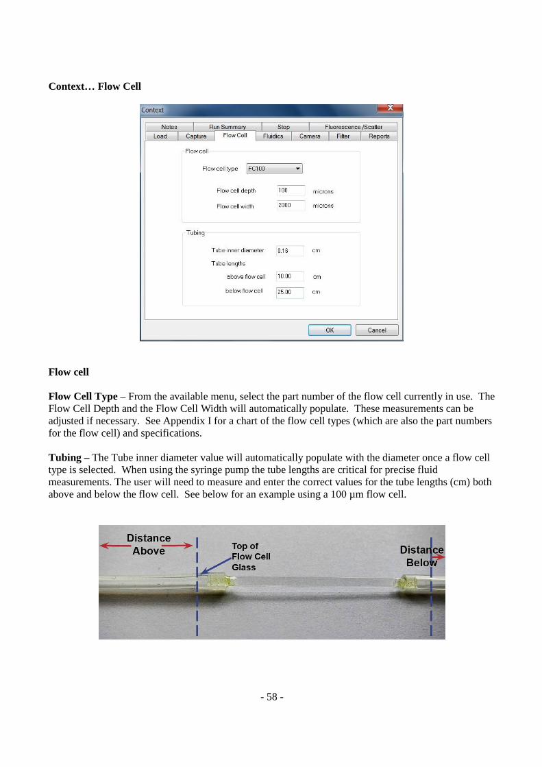
- 58 -

Context… Flow Cell

Flow cell Flow Cell Type – From the available menu, select the part number of the flow cell currently in use. The Flow Cell Depth and the Flow Cell Width will automatically populate. These measurements can be adjusted if necessary. See Appendix I for a chart of the flow cell types (which are also the part numbers for the flow cell) and specifications. Tubing – The Tube inner diameter value will automatically populate with the diameter once a flow cell type is selected. When using the syringe pump the tube lengths are critical for precise fluid measurements. The user will need to measure and enter the correct values for the tube lengths (cm) both above and below the flow cell. See below for an example using a 100 µm flow cell.

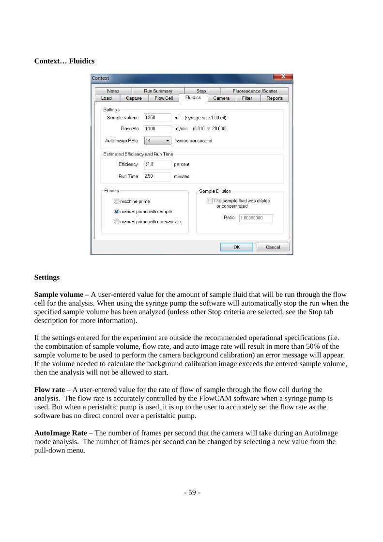
- 59 -

Context… Fluidics

Settings Sample volume – A user-entered value for the amount of sample fluid that will be run through the flow cell for the analysis. When using the syringe pump the software will automatically stop the run when the specified sample volume has been analyzed (unless other Stop criteria are selected, see the Stop tab description for more information). If the settings entered for the experiment are outside the recommended operational specifications (i.e. the combination of sample volume, flow rate, and auto image rate will result in more than 50% of the sample volume to be used to perform the camera background calibration) an error message will appear. If the volume needed to calculate the background calibration image exceeds the entered sample volume, then the analysis will not be allowed to start. Flow rate – A user-entered value for the rate of flow of sample through the flow cell during the analysis. The flow rate is accurately controlled by the FlowCAM software when a syringe pump is used. But when a peristaltic pump is used, it is up to the user to accurately set the flow rate as the software has no direct control over a peristaltic pump. AutoImage Rate – The number of frames per second that the camera will take during an AutoImage mode analysis. The number of frames per second can be changed by selecting a new value from the pull-down menu.

- 60 -

Estimated Efficiency and Run Time Efficiency (%) and Run Time (minutes) are automatically calculated based upon the values entered in the Settings section. If the calculated efficiency percentage results in a situation where multi-imaging of particles is likely to occur, an error message will be displayed. The Flow Rate and/or the AutoImage Rate will need to be adjusted to produce a set of conditions that does not potentially result in the multi-imaging of particles. For standard (not field-of-view) flow cells, the Efficiency can not reach 100% due to the width of the flow cell (which will have areas outside of the camera’s field of view). To obtain Efficiency values that approach 100%, a field-of-view flow cell must be utilized as the fluid channel lies entirely in the camera’s field of view. Finally, the calculators on this screen are provided when a syringe pump is not installed but in that scenario their accuracy depends of the accuracy of the user-provided flow rate. Priming Machine Prime – Automatically pulls sample from the sample introduction port (pipette tip or funnel) into the flow cell and into the camera’s field of view. In order for Machine Prime to function correctly, which was designed using a fluid with a viscosity similar to water, there are two items to check before use:

· Ensure that the tube lengths (both above and below the flow cell) are measured accurately. It is recommended that a minimum resolution of 0.25 cm be used when inputting these lengths.

· When adding the sample into the introduction port (pipette tip or funnel) ensure that the bottom

or leading meniscus of the sample is located between the top of the flow cell tube and the bottom of the pipette or funnel tip. The position of the sample is important as it will allow the correct amount of volume to be drawn down to the flow cell. If the sample level is above the top of the flow cell tube, then there is a risk of imaging a dry flow cell at the start of the run. If the sample level is below the bottom of the pipette tip, then the system may run out of sample before the analysis is complete.

Manual Prime with Sample – The sample has already been drawn into the imaging path in the flow cell. Manual Prime with Non-Sample – A buffer solution, such as distilled water, that contains no sample of interest is drawn into the flow cell and the sample to be tested is added above/on top of this buffer. When a non-sample priming fluid is used before running the sample of interest, the resulting dilution of the target sample is accounted for by the software. If using a non-syringe pump, this priming method will result in the most accurate particle count. Note that the length of the tubing from the sample introduction vessel (funnel or pipette tip) to the top of the flow cell must be measured (cm) and entered correctly. Sample Dilution The sample fluid was diluted or concentrated - This Dilution ratio is used to account for sample dilution or concentration. For example, if a sample is diluted to 50% of the original concentration, this value should be set to 0.5000 to allow the software to correctly calculate statistics on the original concentration.

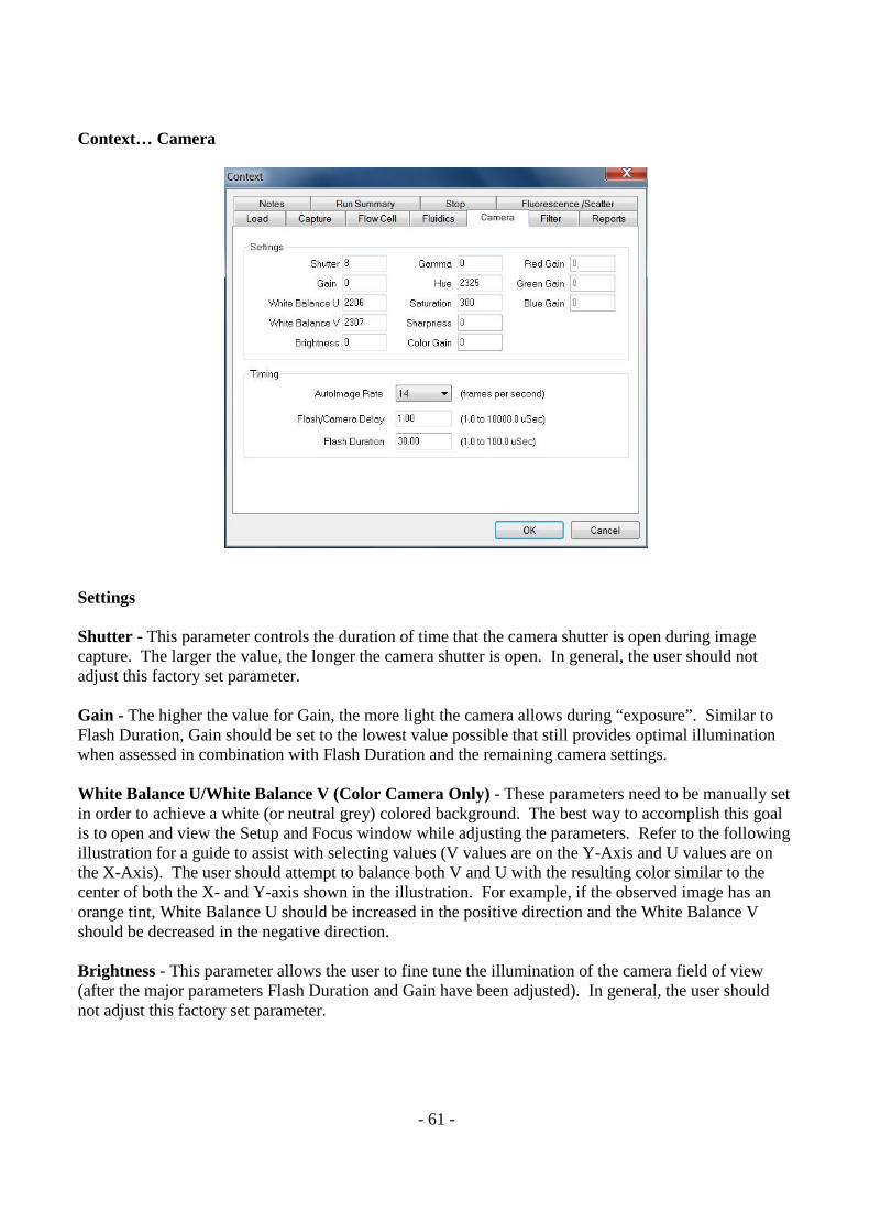
- 61 -

Context… Camera

Settings Shutter - This parameter controls the duration of time that the camera shutter is open during image capture. The larger the value, the longer the camera shutter is open. In general, the user should not adjust this factory set parameter. Gain - The higher the value for Gain, the more light the camera allows during “exposure”. Similar to Flash Duration, Gain should be set to the lowest value possible that still provides optimal illumination when assessed in combination with Flash Duration and the remaining camera settings. White Balance U/White Balance V (Color Camera Only) - These parameters need to be manually set in order to achieve a white (or neutral grey) colored background. The best way to accomplish this goal is to open and view the Setup and Focus window while adjusting the parameters. Refer to the following illustration for a guide to assist with selecting values (V values are on the Y-Axis and U values are on the X-Axis). The user should attempt to balance both V and U with the resulting color similar to the center of both the X- and Y-axis shown in the illustration. For example, if the observed image has an orange tint, White Balance U should be increased in the positive direction and the White Balance V should be decreased in the negative direction. Brightness - This parameter allows the user to fine tune the illumination of the camera field of view (after the major parameters Flash Duration and Gain have been adjusted). In general, the user should not adjust this factory set parameter.

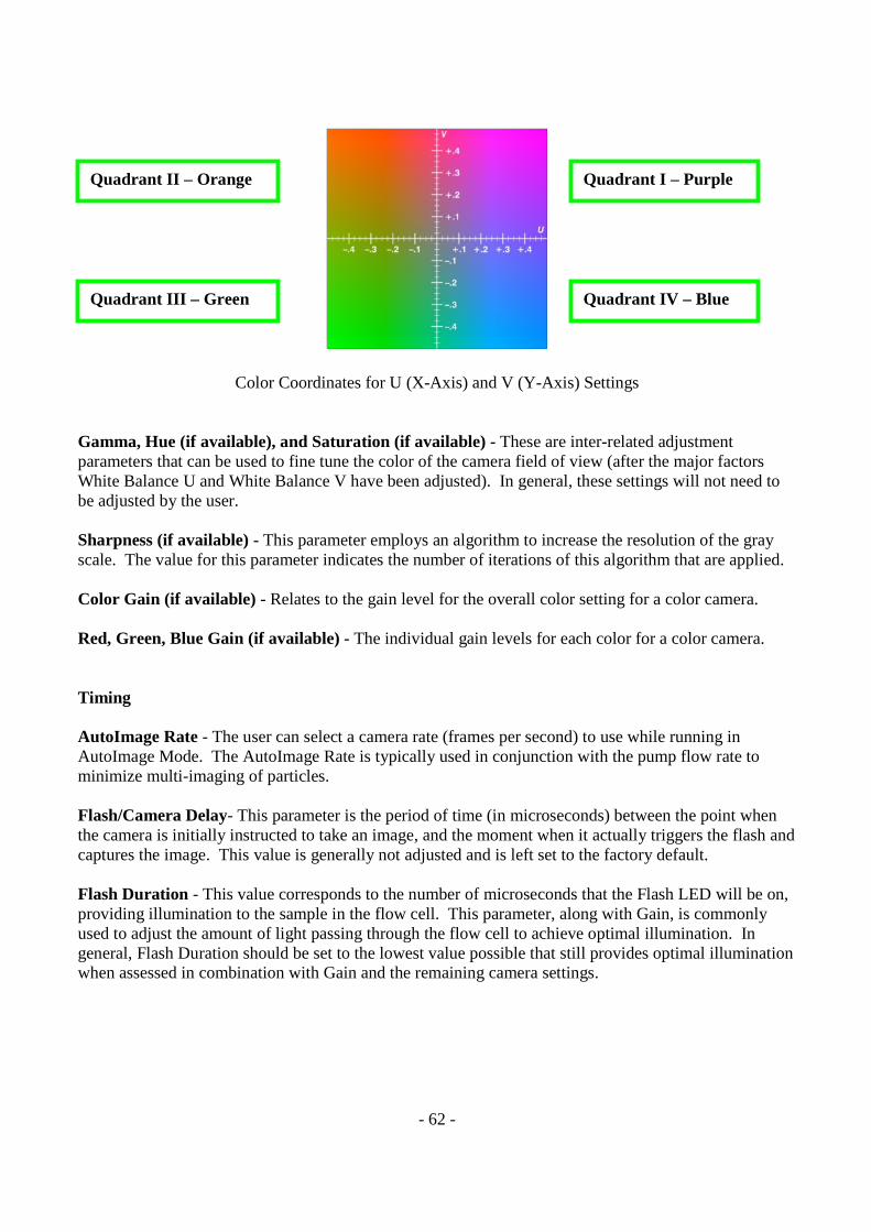
- 62 -

Color Coordinates for U (X-Axis) and V (Y-Axis) Settings Gamma, Hue (if available), and Saturation (if available) - These are inter-related adjustment parameters that can be used to fine tune the color of the camera field of view (after the major factors White Balance U and White Balance V have been adjusted). In general, these settings will not need to be adjusted by the user. Sharpness (if available) - This parameter employs an algorithm to increase the resolution of the gray scale. The value for this parameter indicates the number of iterations of this algorithm that are applied. Color Gain (if available) - Relates to the gain level for the overall color setting for a color camera. Red, Green, Blue Gain (if available) - The individual gain levels for each color for a color camera. Timing AutoImage Rate - The user can select a camera rate (frames per second) to use while running in AutoImage Mode. The AutoImage Rate is typically used in conjunction with the pump flow rate to minimize multi-imaging of particles. Flash/Camera Delay- This parameter is the period of time (in microseconds) between the point when the camera is initially instructed to take an image, and the moment when it actually triggers the flash and captures the image. This value is generally not adjusted and is left set to the factory default. Flash Duration - This value corresponds to the number of microseconds that the Flash LED will be on, providing illumination to the sample in the flow cell. This parameter, along with Gain, is commonly used to adjust the amount of light passing through the flow cell to achieve optimal illumination. In general, Flash Duration should be set to the lowest value possible that still provides optimal illumination when assessed in combination with Gain and the remaining camera settings.

Quadrant II – Orange

Quadrant III – Green

Quadrant I – Purple

Quadrant IV – Blue

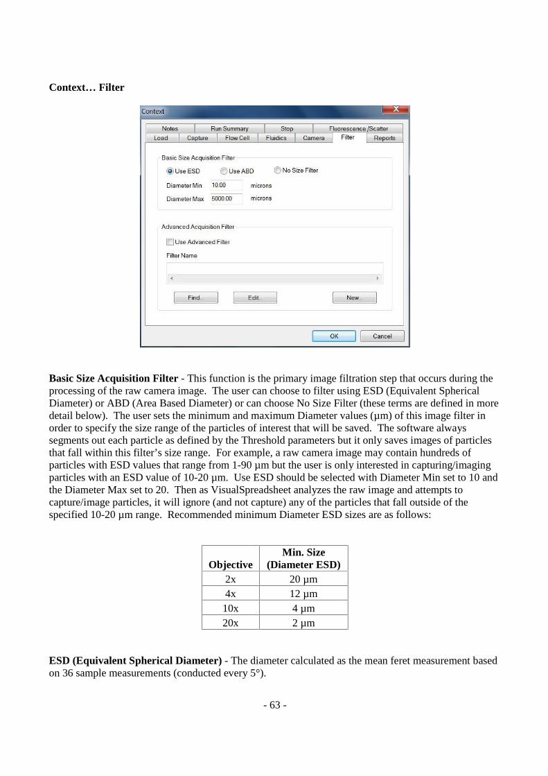
- 63 -

Context… Filter

Basic Size Acquisition Filter - This function is the primary image filtration step that occurs during the processing of the raw camera image. The user can choose to filter using ESD (Equivalent Spherical Diameter) or ABD (Area Based Diameter) or can choose No Size Filter (these terms are defined in more detail below). The user sets the minimum and maximum Diameter values (µm) of this image filter in order to specify the size range of the particles of interest that will be saved. The software always segments out each particle as defined by the Threshold parameters but it only saves images of particles that fall within this filter’s size range. For example, a raw camera image may contain hundreds of particles with ESD values that range from 1-90 µm but the user is only interested in capturing/imaging particles with an ESD value of 10-20 µm. Use ESD should be selected with Diameter Min set to 10 and the Diameter Max set to 20. Then as VisualSpreadsheet analyzes the raw image and attempts to capture/image particles, it will ignore (and not capture) any of the particles that fall outside of the specified 10-20 µm range. Recommended minimum Diameter ESD sizes are as follows:

Objective Min. Size

(Diameter ESD) 2x 20 µm 4x 12 µm 10x 4 µm 20x 2 µm

ESD (Equivalent Spherical Diameter) - The diameter calculated as the mean feret measurement based on 36 sample measurements (conducted every 5°).

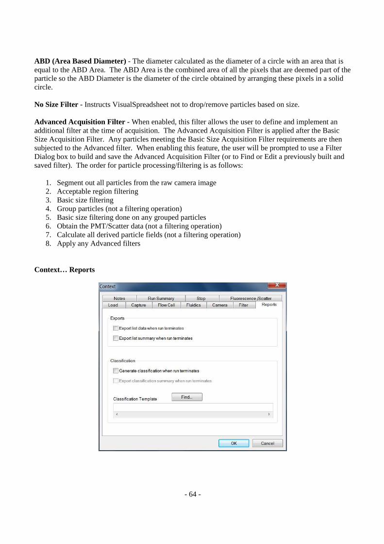
- 64 -

ABD (Area Based Diameter) - The diameter calculated as the diameter of a circle with an area that is equal to the ABD Area. The ABD Area is the combined area of all the pixels that are deemed part of the particle so the ABD Diameter is the diameter of the circle obtained by arranging these pixels in a solid circle. No Size Filter - Instructs VisualSpreadsheet not to drop/remove particles based on size. Advanced Acquisition Filter - When enabled, this filter allows the user to define and implement an additional filter at the time of acquisition. The Advanced Acquisition Filter is applied after the Basic Size Acquisition Filter. Any particles meeting the Basic Size Acquisition Filter requirements are then subjected to the Advanced filter. When enabling this feature, the user will be prompted to use a Filter Dialog box to build and save the Advanced Acquisition Filter (or to Find or Edit a previously built and saved filter). The order for particle processing/filtering is as follows:

1. Segment out all particles from the raw camera image 2. Acceptable region filtering 3. Basic size filtering 4. Group particles (not a filtering operation) 5. Basic size filtering done on any grouped particles 6. Obtain the PMT/Scatter data (not a filtering operation) 7. Calculate all derived particle fields (not a filtering operation) 8. Apply any Advanced filters

Context… Reports

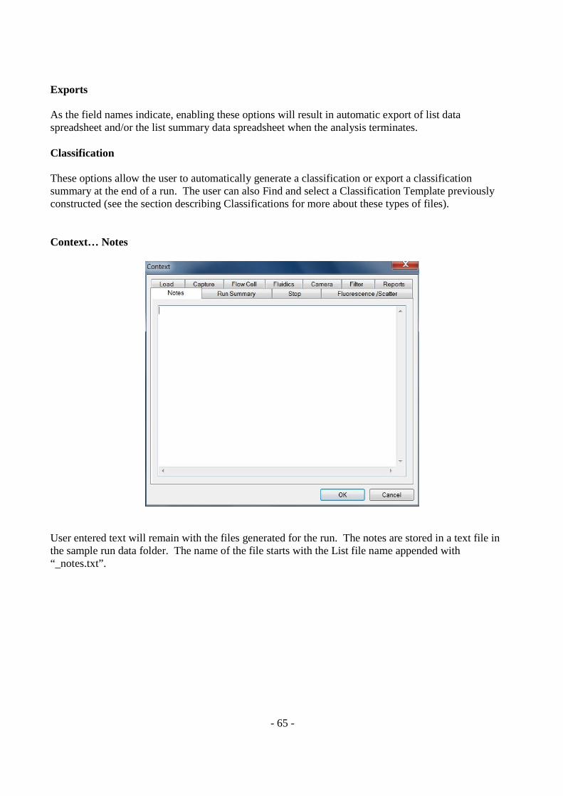
- 65 -

Exports As the field names indicate, enabling these options will result in automatic export of list data spreadsheet and/or the list summary data spreadsheet when the analysis terminates. Classification These options allow the user to automatically generate a classification or export a classification summary at the end of a run. The user can also Find and select a Classification Template previously constructed (see the section describing Classifications for more about these types of files).

Context… Notes

User entered text will remain with the files generated for the run. The notes are stored in a text file in the sample run data folder. The name of the file starts with the List file name appended with “_notes.txt”.

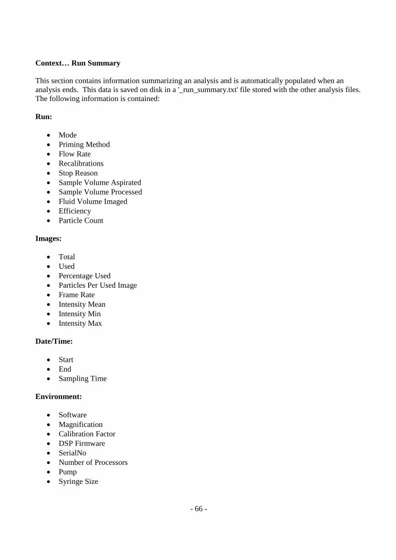
- 66 -

Context… Run Summary This section contains information summarizing an analysis and is automatically populated when an analysis ends. This data is saved on disk in a '_run_summary.txt' file stored with the other analysis files. The following information is contained: Run:

· Mode · Priming Method · Flow Rate · Recalibrations · Stop Reason · Sample Volume Aspirated · Sample Volume Processed · Fluid Volume Imaged · Efficiency · Particle Count

Images:

· Total · Used · Percentage Used · Particles Per Used Image · Frame Rate · Intensity Mean · Intensity Min · Intensity Max

Date/Time:

· Start · End · Sampling Time

Environment:

· Software · Magnification · Calibration Factor · DSP Firmware · SerialNo · Number of Processors · Pump · Syringe Size

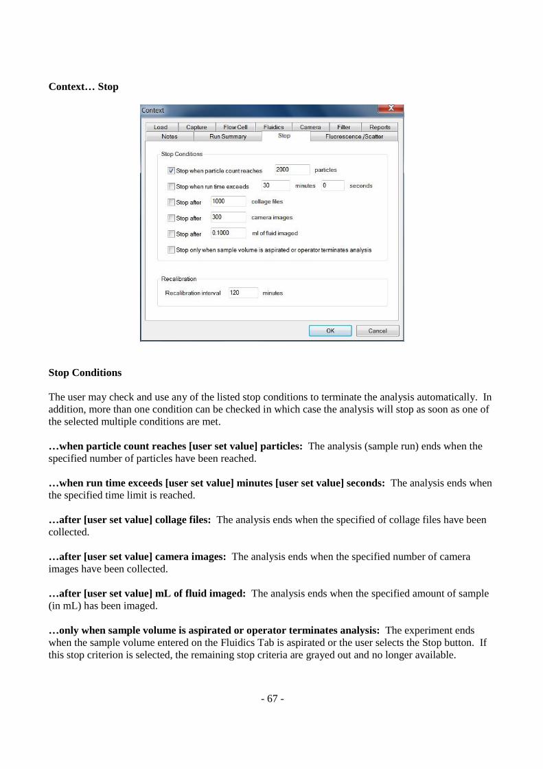
- 67 -

Context… Stop

Stop Conditions The user may check and use any of the listed stop conditions to terminate the analysis automatically. In addition, more than one condition can be checked in which case the analysis will stop as soon as one of the selected multiple conditions are met. …when particle count reaches [user set value] particles: The analysis (sample run) ends when the specified number of particles have been reached. …when run time exceeds [user set value] minutes [user set value] seconds: The analysis ends when the specified time limit is reached. …after [user set value] collage files: The analysis ends when the specified of collage files have been collected. …after [user set value] camera images: The analysis ends when the specified number of camera images have been collected. …after [user set value] mL of fluid imaged: The analysis ends when the specified amount of sample (in mL) has been imaged. …only when sample volume is aspirated or operator terminates analysis: The experiment ends when the sample volume entered on the Fluidics Tab is aspirated or the user selects the Stop button. If this stop criterion is selected, the remaining stop criteria are grayed out and no longer available.

- 68 -

Recalibration …interval [user set value] minutes: This setting determines the frequency of recalibration. A recalibration consists of collecting a new set of calibration images, averaging them, and producing a new composite calibration image. This is the same process that automatically occurs at the start of an analysis. Recalibration can be helpful if the sample in question has a tendency to adhere to the glass surfaces of the flow cell resulting in erroneous repeat imaging of the same particles. Context… Fluorescence/Scatter

This section allows the user to select and refine the settings for the Trigger Modes of the FlowCAM if the unit in question is a model equipped to run in Trigger Mode. See Section Two for more information on Trigger Mode. Channel 1 and Channel 2: These are the two channels that utilize PMTs to detect fluorescence signals from particles in the sample that fluoresce (see Figure 2, letter B). The standard configuration for Channels 1 and 2 is: Channel 1 is the >650 nm PMT and Channel 2 is the PMT for the 575 nm filter. Scatter: This channel uses the Scatter Detector (see Figure 2, letter H) to detect the scatter of laser light by particles in the sample. Each one of the above three options can be utilized in two different modes. Each channel can be set to Trigger or Measure. When set to Trigger, the FlowCAM will be triggered to take a camera image when a particle produces a signal (fluorescence or laser light scatter) that meets or exceeds the user defined Threshold (see below for more information on Threshold). When set to measure, the FlowCAM will only monitor and record the values detected on these channels but will not trigger the camera based on

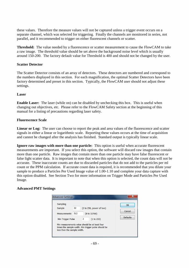
- 69 -

these values. Therefore the measure values will not be captured unless a trigger event occurs on a separate channel, which was selected for triggering. Finally the channels are monitored in series, not parallel, and it recommended to trigger on either fluorescent channels or scatter. Threshold: The value needed by a fluorescence or scatter measurement to cause the FlowCAM to take a raw image. The threshold value should be set above the background noise level which is usually around 150-200. The factory default value for Threshold is 400 and should not be changed by the user. Scatter Detector The Scatter Detector consists of an array of detectors. These detectors are numbered and correspond to the numbers displayed in this section. For each magnification, the optimal Scatter Detectors have been factory determined and preset in this section. Typically, the FlowCAM user should not adjust these settings. Laser Enable Laser: The laser (while on) can be disabled by unchecking this box. This is useful when changing out objectives, etc. Please refer to the FlowCAM Safety section at the beginning of this manual for a listing of precautions regarding laser safety. Fluorescence Scale Linear or Log: The user can choose to report the peak and area values of the fluorescence and scatter signals in either a linear or logarithmic scale. Reporting these values occurs at the time of acquisition and cannot be changed after the analysis has finished. Standard output is typically linear scale. Ignore raw images with more than one particle: This option is useful when accurate fluorescent measurements are important. If you select this option, the software will discard raw images that contain more than one particle. Raw images that contain more than one particle may have false fluorescent or false light scatter data. It is important to note that when this option is selected, the count data will not be accurate. These inaccurate counts are due to discarded particles that do not add to the particles per ml count or the PPM calculation. If accurate count data is required, it is recommended that you dilute your sample to produce a Particles Per Used Image value of 1.00-1.10 and complete your data capture with this option disabled. See Section Two for more information on Trigger Mode and Particles Per Used Image. Advanced PMT Settings

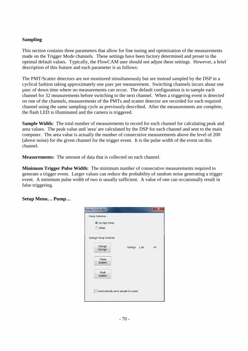
- 70 -

Sampling This section contains three parameters that allow for fine tuning and optimization of the measurements made on the Trigger Mode channels. These settings have been factory determined and preset to the optimal default values. Typically, the FlowCAM user should not adjust these settings. However, a brief description of this feature and each parameter is as follows: The PMT/Scatter detectors are not monitored simultaneously but are instead sampled by the DSP in a cyclical fashion taking approximately one µsec per measurement. Switching channels incurs about one µsec of down time where no measurements can occur. The default configuration is to sample each channel for 32 measurements before switching to the next channel. When a triggering event is detected on one of the channels, measurements of the PMTs and scatter detector are recorded for each required channel using the same sampling cycle as previously described. After the measurements are complete, the flash LED is illuminated and the camera is triggered. Sample Width: The total number of measurements to record for each channel for calculating peak and area values. The peak value and 'area' are calculated by the DSP for each channel and sent to the main computer. The area value is actually the number of consecutive measurements above the level of 200 (above noise) for the given channel for the trigger event. It is the pulse width of the event on this channel. Measurements: The amount of data that is collected on each channel. Minimum Trigger Pulse Width: The minimum number of consecutive measurements required to generate a trigger event. Larger values can reduce the probability of random noise generating a trigger event. A minimum pulse width of two is usually sufficient. A value of one can occasionally result in false triggering.

Setup Menu… Pump…

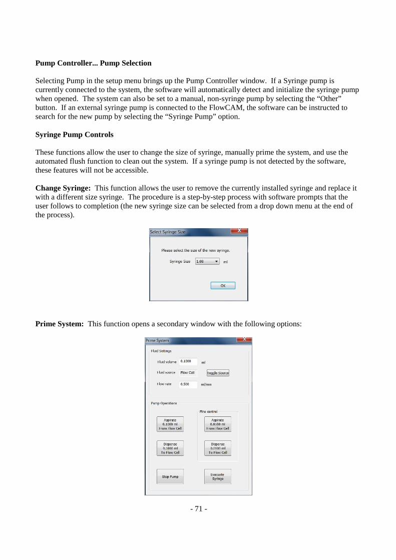
- 71 -

Pump Controller... Pump Selection Selecting Pump in the setup menu brings up the Pump Controller window. If a Syringe pump is currently connected to the system, the software will automatically detect and initialize the syringe pump when opened. The system can also be set to a manual, non-syringe pump by selecting the “Other” button. If an external syringe pump is connected to the FlowCAM, the software can be instructed to search for the new pump by selecting the “Syringe Pump” option. Syringe Pump Controls These functions allow the user to change the size of syringe, manually prime the system, and use the automated flush function to clean out the system. If a syringe pump is not detected by the software, these features will not be accessible. Change Syringe: This function allows the user to remove the currently installed syringe and replace it with a different size syringe. The procedure is a step-by-step process with software prompts that the user follows to completion (the new syringe size can be selected from a drop down menu at the end of the process).

Prime System: This function opens a secondary window with the following options:

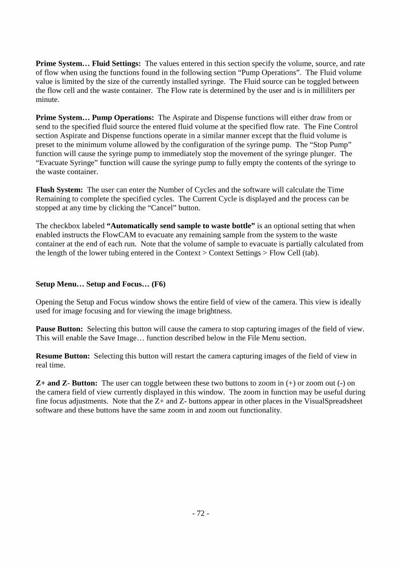
- 72 -

Prime System… Fluid Settings: The values entered in this section specify the volume, source, and rate of flow when using the functions found in the following section “Pump Operations”. The Fluid volume value is limited by the size of the currently installed syringe. The Fluid source can be toggled between the flow cell and the waste container. The Flow rate is determined by the user and is in milliliters per minute. Prime System… Pump Operations: The Aspirate and Dispense functions will either draw from or send to the specified fluid source the entered fluid volume at the specified flow rate. The Fine Control section Aspirate and Dispense functions operate in a similar manner except that the fluid volume is preset to the minimum volume allowed by the configuration of the syringe pump. The “Stop Pump” function will cause the syringe pump to immediately stop the movement of the syringe plunger. The “Evacuate Syringe” function will cause the syringe pump to fully empty the contents of the syringe to the waste container. Flush System: The user can enter the Number of Cycles and the software will calculate the Time Remaining to complete the specified cycles. The Current Cycle is displayed and the process can be stopped at any time by clicking the “Cancel” button. The checkbox labeled “Automatically send sample to waste bottle” is an optional setting that when enabled instructs the FlowCAM to evacuate any remaining sample from the system to the waste container at the end of each run. Note that the volume of sample to evacuate is partially calculated from the length of the lower tubing entered in the Context > Context Settings > Flow Cell (tab).

Setup Menu… Setup and Focus… (F6) Opening the Setup and Focus window shows the entire field of view of the camera. This view is ideally used for image focusing and for viewing the image brightness. Pause Button: Selecting this button will cause the camera to stop capturing images of the field of view. This will enable the Save Image… function described below in the File Menu section. Resume Button: Selecting this button will restart the camera capturing images of the field of view in real time. Z+ and Z- Button: The user can toggle between these two buttons to zoom in (+) or zoom out (-) on the camera field of view currently displayed in this window. The zoom in function may be useful during fine focus adjustments. Note that the Z+ and Z- buttons appear in other places in the VisualSpreadsheet software and these buttons have the same zoom in and zoom out functionality.

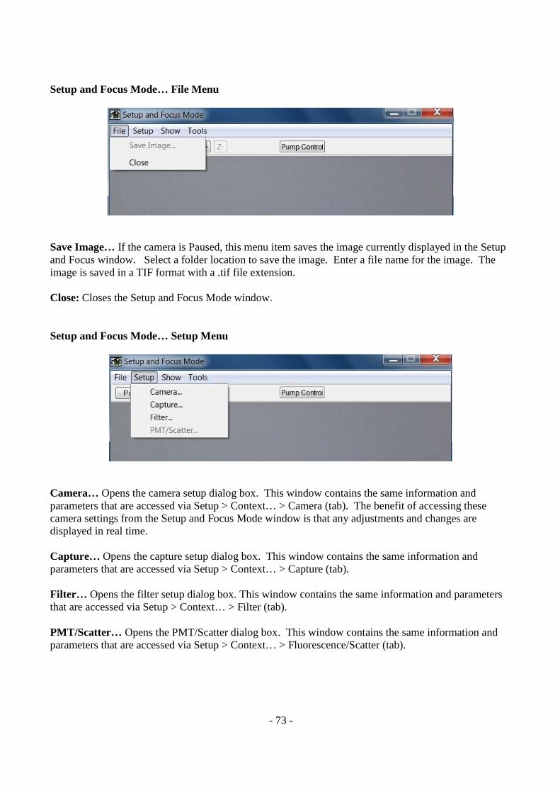
- 73 -

Setup and Focus Mode… File Menu

Save Image… If the camera is Paused, this menu item saves the image currently displayed in the Setup and Focus window. Select a folder location to save the image. Enter a file name for the image. The image is saved in a TIF format with a .tif file extension. Close: Closes the Setup and Focus Mode window. Setup and Focus Mode… Setup Menu

Camera… Opens the camera setup dialog box. This window contains the same information and parameters that are accessed via Setup > Context… > Camera (tab). The benefit of accessing these camera settings from the Setup and Focus Mode window is that any adjustments and changes are displayed in real time. Capture… Opens the capture setup dialog box. This window contains the same information and parameters that are accessed via Setup > Context… > Capture (tab). Filter… Opens the filter setup dialog box. This window contains the same information and parameters that are accessed via Setup > Context… > Filter (tab).

PMT/Scatter… Opens the PMT/Scatter dialog box. This window contains the same information and parameters that are accessed via Setup > Context… > Fluorescence/Scatter (tab).

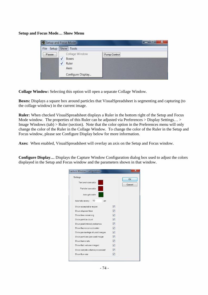
- 74 -

Setup and Focus Mode… Show Menu

Collage Window: Selecting this option will open a separate Collage Window. Boxes: Displays a square box around particles that VisualSpreadsheet is segmenting and capturing (to the collage window) in the current image. Ruler: When checked VisualSpreadsheet displays a Ruler in the bottom right of the Setup and Focus Mode window. The properties of this Ruler can be adjusted via Preferences > Display Settings… > Image Windows (tab) > Ruler (section). Note that the color option in the Preferences menu will only change the color of the Ruler in the Collage Window. To change the color of the Ruler in the Setup and Focus window, please see Configure Display below for more information. Axes: When enabled, VisualSpreadsheet will overlay an axis on the Setup and Focus window. Configure Display… Displays the Capture Window Configuration dialog box used to adjust the colors displayed in the Setup and Focus window and the parameters shown in that window.

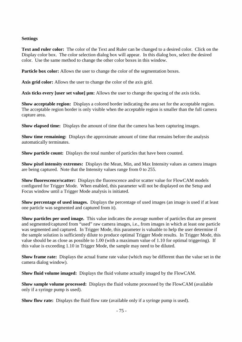
- 75 -

Settings Text and ruler color: The color of the Text and Ruler can be changed to a desired color. Click on the Display color box. The color selection dialog box will appear. In this dialog box, select the desired color. Use the same method to change the other color boxes in this window. Particle box color: Allows the user to change the color of the segmentation boxes. Axis grid color: Allows the user to change the color of the axis grid. Axis ticks every [user set value] µm: Allows the user to change the spacing of the axis ticks. Show acceptable region: Displays a colored border indicating the area set for the acceptable region. The acceptable region border is only visible when the acceptable region is smaller than the full camera capture area. Show elapsed time: Displays the amount of time that the camera has been capturing images. Show time remaining: Displays the approximate amount of time that remains before the analysis automatically terminates. Show particle count: Displays the total number of particles that have been counted. Show pixel intensity extremes: Displays the Mean, Min, and Max Intensity values as camera images are being captured. Note that the Intensity values range from 0 to 255. Show fluorescence/scatter: Displays the fluorescence and/or scatter value for FlowCAM models configured for Trigger Mode. When enabled, this parameter will not be displayed on the Setup and Focus window until a Trigger Mode analysis is initiated. Show percentage of used images. Displays the percentage of used images (an image is used if at least one particle was segmented and captured from it). Show particles per used image. This value indicates the average number of particles that are present and segmented/captured from “used” raw camera images, i.e., from images in which at least one particle was segmented and captured. In Trigger Mode, this parameter is valuable to help the user determine if the sample solution is sufficiently dilute to produce optimal Trigger Mode results. In Trigger Mode, this value should be as close as possible to 1.00 (with a maximum value of 1.10 for optimal triggering). If this value is exceeding 1.10 in Trigger Mode, the sample may need to be diluted. Show frame rate: Displays the actual frame rate value (which may be different than the value set in the camera dialog window). Show fluid volume imaged: Displays the fluid volume actually imaged by the FlowCAM. Show sample volume processed: Displays the fluid volume processed by the FlowCAM (available only if a syringe pump is used). Show flow rate: Displays the fluid flow rate (available only if a syringe pump is used).

- 76 -

Show Efficiency: Displays the actual efficiency (available only if a syringe pump is used). Setup and Focus Mode… Tools Menu

Recalibrate: This function is not relevant when in Setup and Focus Mode. This function is employed when doing an analysis. During the analysis, the user can select the Recalibrate function on this menu to immediately generate a new calibration image. Reset Frame Rate Counter: This function will reset the frame rate counter (if displayed) to zero. The image count and elapsed run time, if displayed, are also reset. Raw Pixel Intensity… This advanced tool can be used as a guide to help set the illumination uniformity of the image when adjusting either the LED adjustment knob or the camera Gain settings. A Raw Image Pixel Intensity graph is shown that has both a histogram of pixel intensity and the cumulative % for the histogram. The intensity at the lower right hand end of the histogram line shows the maximum intensity. If the intensity is not optimally adjusted, the graph may appear similar to the following example:

Notice the uneven appearance of the histogram line (red). As the intensity is adjusted, the graph should change to look similar to the following example:

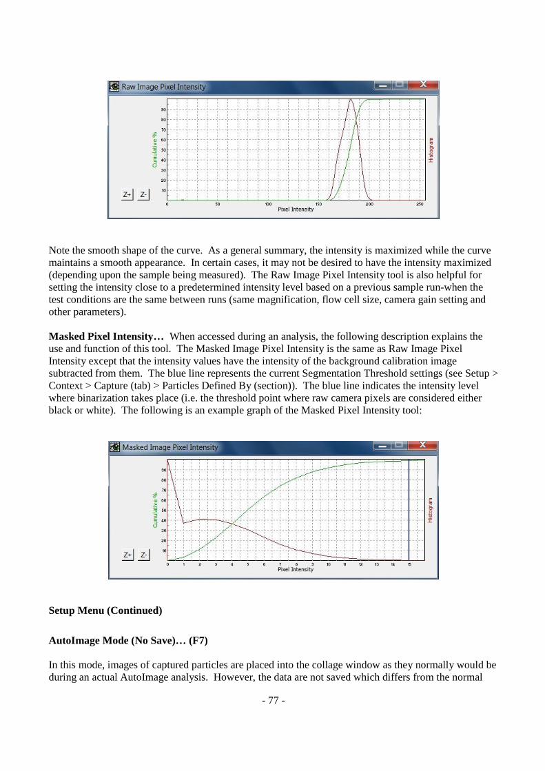
- 77 -

Note the smooth shape of the curve. As a general summary, the intensity is maximized while the curve maintains a smooth appearance. In certain cases, it may not be desired to have the intensity maximized (depending upon the sample being measured). The Raw Image Pixel Intensity tool is also helpful for setting the intensity close to a predetermined intensity level based on a previous sample run-when the test conditions are the same between runs (same magnification, flow cell size, camera gain setting and other parameters). Masked Pixel Intensity… When accessed during an analysis, the following description explains the use and function of this tool. The Masked Image Pixel Intensity is the same as Raw Image Pixel Intensity except that the intensity values have the intensity of the background calibration image subtracted from them. The blue line represents the current Segmentation Threshold settings (see Setup > Context > Capture (tab) > Particles Defined By (section)). The blue line indicates the intensity level where binarization takes place (i.e. the threshold point where raw camera pixels are considered either black or white). The following is an example graph of the Masked Pixel Intensity tool:

Setup Menu (Continued)

AutoImage Mode (No Save)… (F7) In this mode, images of captured particles are placed into the collage window as they normally would be during an actual AutoImage analysis. However, the data are not saved which differs from the normal

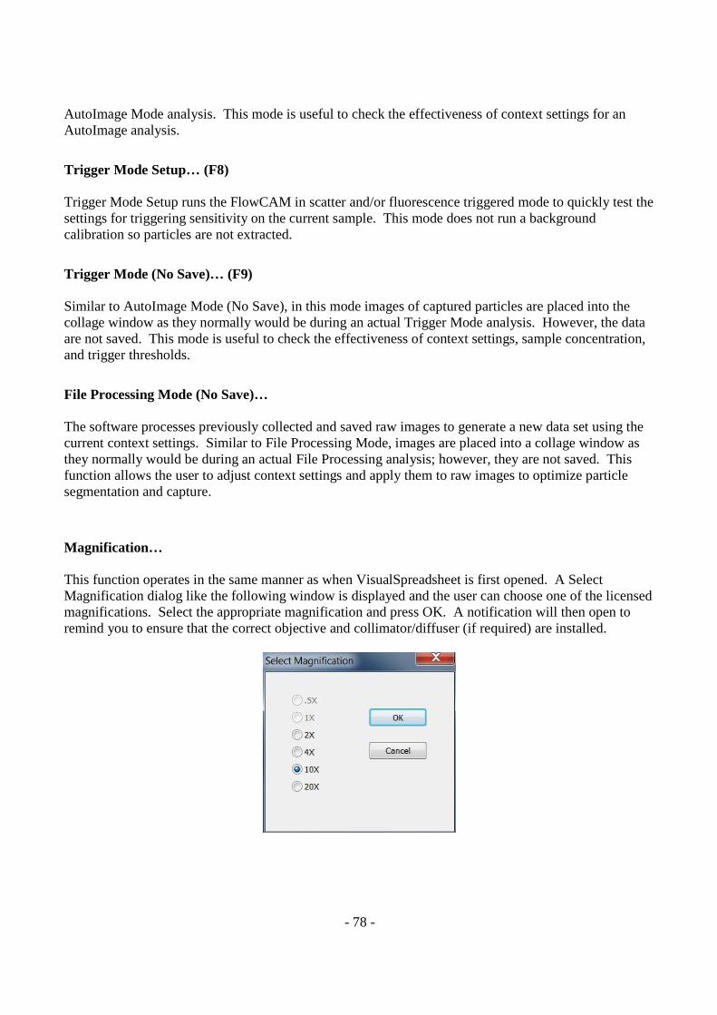
- 78 -

AutoImage Mode analysis. This mode is useful to check the effectiveness of context settings for an AutoImage analysis.

Trigger Mode Setup… (F8) Trigger Mode Setup runs the FlowCAM in scatter and/or fluorescence triggered mode to quickly test the settings for triggering sensitivity on the current sample. This mode does not run a background calibration so particles are not extracted.

Trigger Mode (No Save)… (F9) Similar to AutoImage Mode (No Save), in this mode images of captured particles are placed into the collage window as they normally would be during an actual Trigger Mode analysis. However, the data are not saved. This mode is useful to check the effectiveness of context settings, sample concentration, and trigger thresholds.

File Processing Mode (No Save)… The software processes previously collected and saved raw images to generate a new data set using the current context settings. Similar to File Processing Mode, images are placed into a collage window as they normally would be during an actual File Processing analysis; however, they are not saved. This function allows the user to adjust context settings and apply them to raw images to optimize particle segmentation and capture.

Magnification… This function operates in the same manner as when VisualSpreadsheet is first opened. A Select Magnification dialog like the following window is displayed and the user can choose one of the licensed magnifications. Select the appropriate magnification and press OK. A notification will then open to remind you to ensure that the correct objective and collimator/diffuser (if required) are installed.

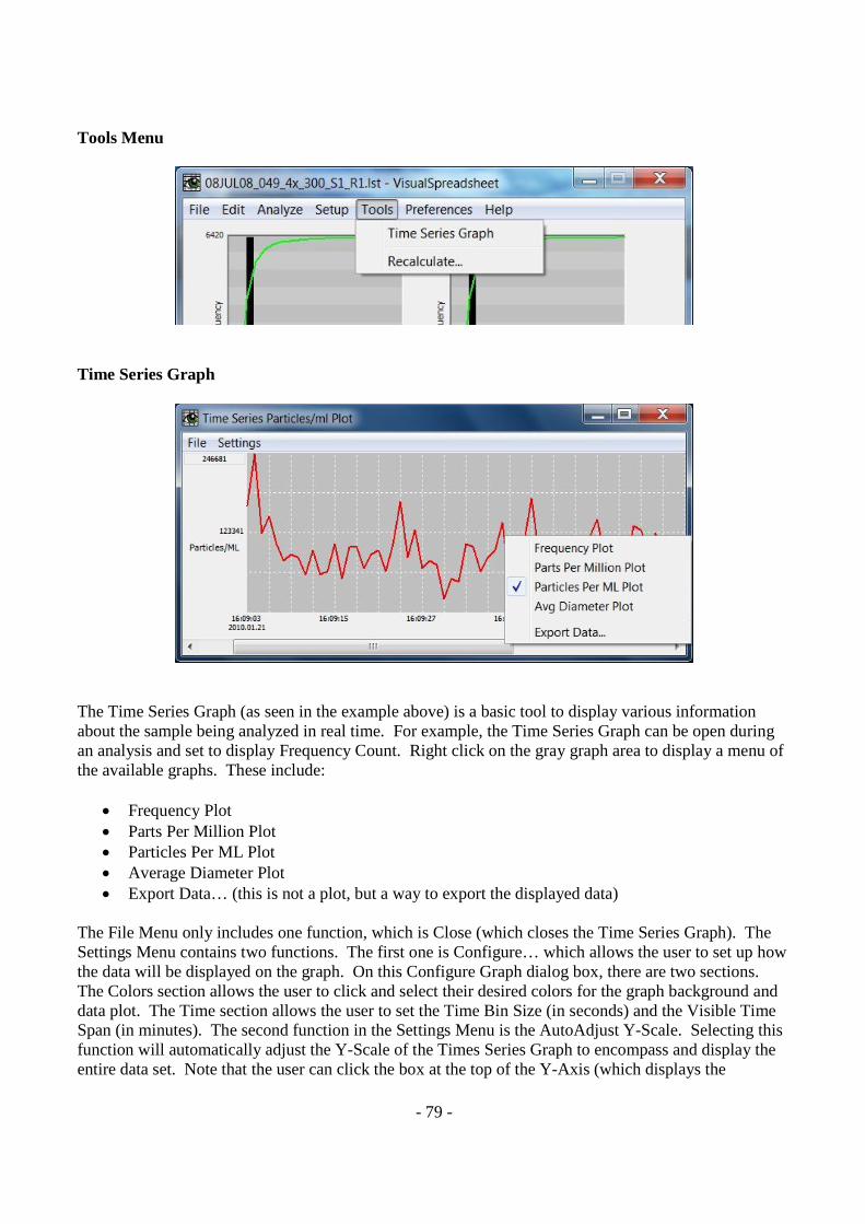
- 79 -

Tools Menu

Time Series Graph

The Time Series Graph (as seen in the example above) is a basic tool to display various information about the sample being analyzed in real time. For example, the Time Series Graph can be open during an analysis and set to display Frequency Count. Right click on the gray graph area to display a menu of the available graphs. These include:

· Frequency Plot · Parts Per Million Plot · Particles Per ML Plot · Average Diameter Plot · Export Data… (this is not a plot, but a way to export the displayed data)

The File Menu only includes one function, which is Close (which closes the Time Series Graph). The Settings Menu contains two functions. The first one is Configure… which allows the user to set up how the data will be displayed on the graph. On this Configure Graph dialog box, there are two sections. The Colors section allows the user to click and select their desired colors for the graph background and data plot. The Time section allows the user to set the Time Bin Size (in seconds) and the Visible Time Span (in minutes). The second function in the Settings Menu is the AutoAdjust Y-Scale. Selecting this function will automatically adjust the Y-Scale of the Times Series Graph to encompass and display the entire data set. Note that the user can click the box at the top of the Y-Axis (which displays the

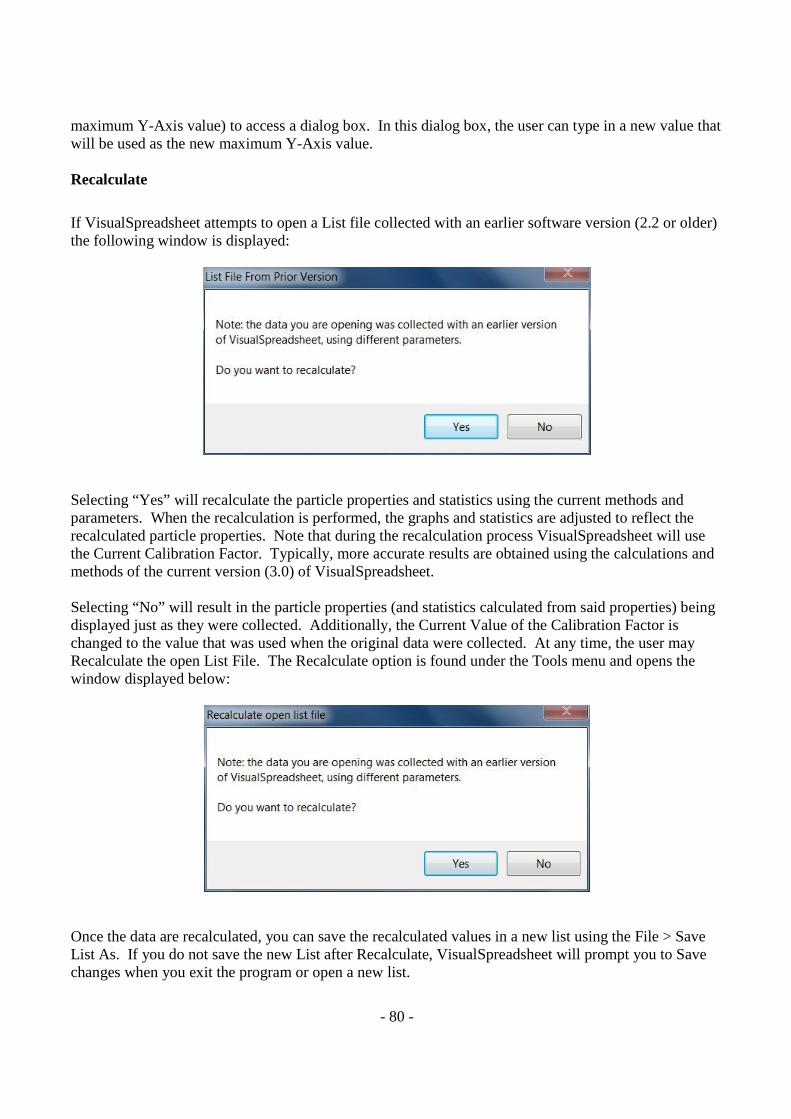
- 80 -

maximum Y-Axis value) to access a dialog box. In this dialog box, the user can type in a new value that will be used as the new maximum Y-Axis value. Recalculate

If VisualSpreadsheet attempts to open a List file collected with an earlier software version (2.2 or older) the following window is displayed:

Selecting “Yes” will recalculate the particle properties and statistics using the current methods and parameters. When the recalculation is performed, the graphs and statistics are adjusted to reflect the recalculated particle properties. Note that during the recalculation process VisualSpreadsheet will use the Current Calibration Factor. Typically, more accurate results are obtained using the calculations and methods of the current version (3.0) of VisualSpreadsheet. Selecting “No” will result in the particle properties (and statistics calculated from said properties) being displayed just as they were collected. Additionally, the Current Value of the Calibration Factor is changed to the value that was used when the original data were collected. At any time, the user may Recalculate the open List File. The Recalculate option is found under the Tools menu and opens the window displayed below:

Once the data are recalculated, you can save the recalculated values in a new list using the File > Save List As. If you do not save the new List after Recalculate, VisualSpreadsheet will prompt you to Save changes when you exit the program or open a new list.

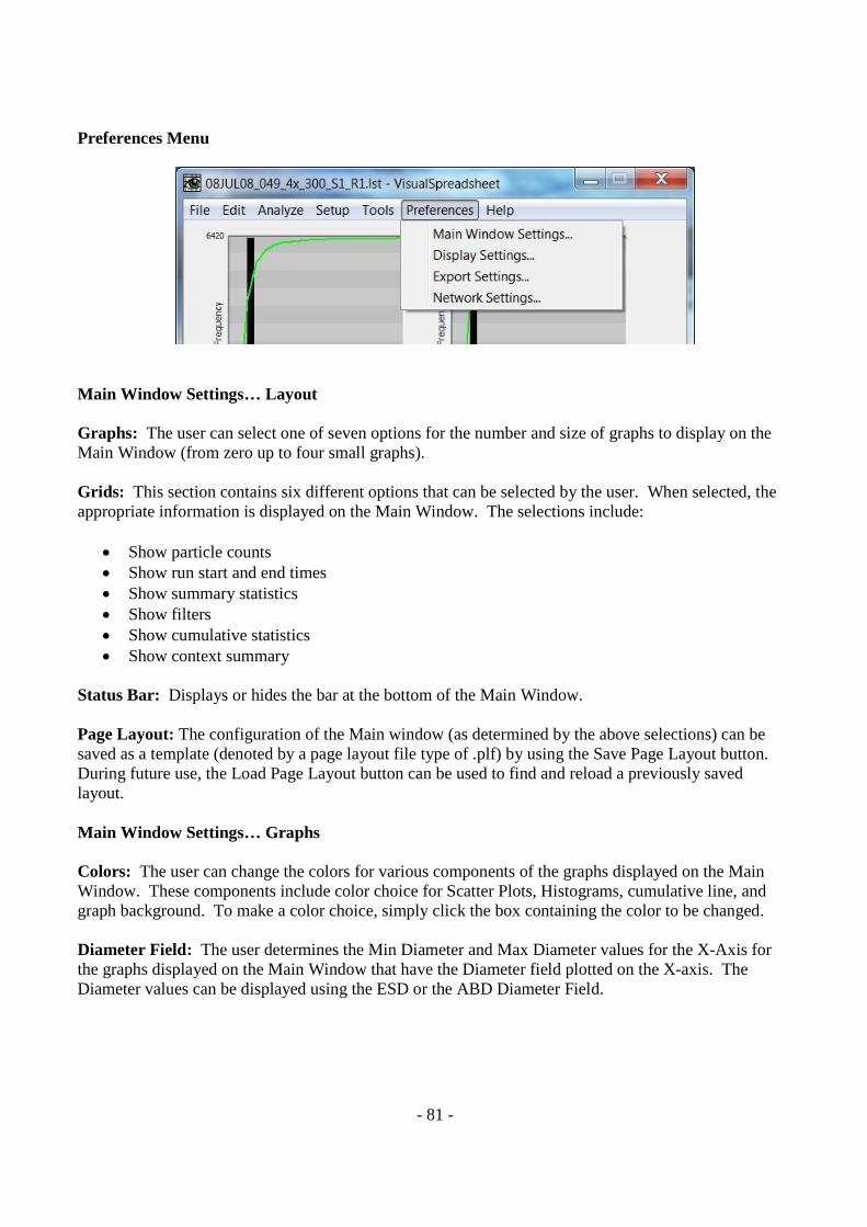
- 81 -

Preferences Menu

Main Window Settings… Layout Graphs: The user can select one of seven options for the number and size of graphs to display on the Main Window (from zero up to four small graphs). Grids: This section contains six different options that can be selected by the user. When selected, the appropriate information is displayed on the Main Window. The selections include:

· Show particle counts · Show run start and end times · Show summary statistics · Show filters · Show cumulative statistics · Show context summary

Status Bar: Displays or hides the bar at the bottom of the Main Window. Page Layout: The configuration of the Main window (as determined by the above selections) can be saved as a template (denoted by a page layout file type of .plf) by using the Save Page Layout button. During future use, the Load Page Layout button can be used to find and reload a previously saved layout. Main Window Settings… Graphs Colors: The user can change the colors for various components of the graphs displayed on the Main Window. These components include color choice for Scatter Plots, Histograms, cumulative line, and graph background. To make a color choice, simply click the box containing the color to be changed. Diameter Field: The user determines the Min Diameter and Max Diameter values for the X-Axis for the graphs displayed on the Main Window that have the Diameter field plotted on the X-axis. The Diameter values can be displayed using the ESD or the ABD Diameter Field.

- 82 -

Histogram Bin Sizes: This section allows the user to modify the bin sizes for the Histograms displayed on the Main Window. The bin sizes that can be adjusted include:

· Diameter · Aspect Ratio or Transparency · Fluorescence or Scatter · Capture Position (X or Y) · Intensity or Edge Gradient

Main Window Settings… Summary Statistics Calculated Values: The user may select which values to display in the columns of the Summary Statistics grid on the Main Window in this section. Values to display include:

· Mean · Minimum · Maximum · Standard Deviation · Coefficient of Variation · D10-D25-D50(Median)-D75-D90

D Values: These values are related to standard sieve techniques and equipment. The Dn value is the value such that n% of the measured values are smaller than Dn and (100 – n)% of the measured values are larger than Dn. For example, the D10 value for diameter is the value such that 10% of the sample particles have a smaller diameter than D10 and 90% have a larger diameter than D10. Similarly, the D10 value for volume is the value such that 10% of the sample particles have a smaller volume than D10 and 90% have a larger volume than D10. D[4,3] (ABD) and D[4,3] (ESD) Values: These values (the volume moment mean of the particle) are the mean diameter computed by weighting the ABD or ESD diameter of each particle by the ABD or ESD volume of the particle. Because of the weights, the particles with large volume influence the mean more than the particles with small volume. Summary Statistics: The user may select which values to display in the rows of the Summary Statistics grid on the Main Window in this section. Values (41 total) to display include: Area (ABD), Aspect Ratio, Average Blue, Average Green, Average Red, Capture X, Capture Y, Ch1 Area, Ch1 Peak, Ch1 Width, Ch2 Area, Ch2 Peak, Ch2 Width, Ch2/Ch1 Ratio, Circle Fit, Compactness, Convex Perimeter, Diameter (ABD), Diameter (ESD), D[4,3] (ABD), D[4,3] (ESD), Edge Gradient, Elongation, Image Height, Image Width, Intensity, Length, Perimeter, Ratio Blue/Green, Ratio Red/Blue, Ratio Red/Green, Roughness, Scatter Area, Scatter Peak, Scatter Width, Sigma Intensity, Sum Intensity, Transparency, Volume (ABD), Volume (ESD), Width

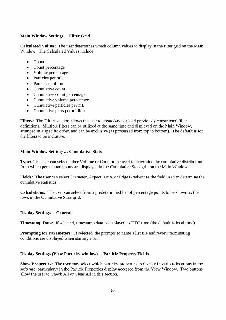
- 83 -

Main Window Settings… Filter Grid Calculated Values: The user determines which column values to display in the filter grid on the Main Window. The Calculated Values include:

· Count · Count percentage · Volume percentage · Particles per mL · Parts per million · Cumulative count · Cumulative count percentage · Cumulative volume percentage · Cumulative particles per mL · Cumulative parts per million

Filters: The Filters section allows the user to create/save or load previously constructed filter definitions. Multiple filters can be utilized at the same time and displayed on the Main Window, arranged in a specific order, and can be exclusive (as processed from top to bottom). The default is for the filters to be inclusive. Main Window Settings… Cumulative Stats Type: The user can select either Volume or Count to be used to determine the cumulative distribution from which percentage points are displayed in the Cumulative Stats grid on the Main Window. Fields: The user can select Diameter, Aspect Ratio, or Edge Gradient as the field used to determine the cumulative statistics. Calculations: The user can select from a predetermined list of percentage points to be shown as the rows of the Cumulative Stats grid. Display Settings… General Timestamp Data: If selected, timestamp data is displayed as UTC time (the default is local time). Prompting for Parameters: If selected, the prompts to name a list file and review terminating conditions are displayed when starting a run. Display Settings (View Particles window)… Particle Property Fields

Show Properties: The user may select which particles properties to display in various locations in the software, particularly in the Particle Properties display accessed from the View Window. Two buttons allow the user to Check All or Clear All in this section.

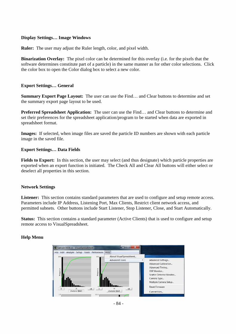
- 84 -

Display Settings… Image Windows Ruler: The user may adjust the Ruler length, color, and pixel width. Binarization Overlay: The pixel color can be determined for this overlay (i.e. for the pixels that the software determines constitute part of a particle) in the same manner as for other color selections. Click the color box to open the Color dialog box to select a new color. Export Settings… General Summary Export Page Layout: The user can use the Find… and Clear buttons to determine and set the summary export page layout to be used. Preferred Spreadsheet Application: The user can use the Find… and Clear buttons to determine and set their preferences for the spreadsheet application/program to be started when data are exported in spreadsheet format. Images: If selected, when image files are saved the particle ID numbers are shown with each particle image in the saved file. Export Settings… Data Fields

Fields to Export: In this section, the user may select (and thus designate) which particle properties are exported when an export function is initiated. The Check All and Clear All buttons will either select or deselect all properties in this section. Network Settings Listener: This section contains standard parameters that are used to configure and setup remote access. Parameters include IP Address, Listening Port, Max Clients, Restrict client network access, and permitted subnets. Other buttons include Start Listener, Stop Listener, Close, and Start Automatically. Status: This section contains a standard parameter (Active Clients) that is used to configure and setup remote access to VisualSpreadsheet.

Help Menu

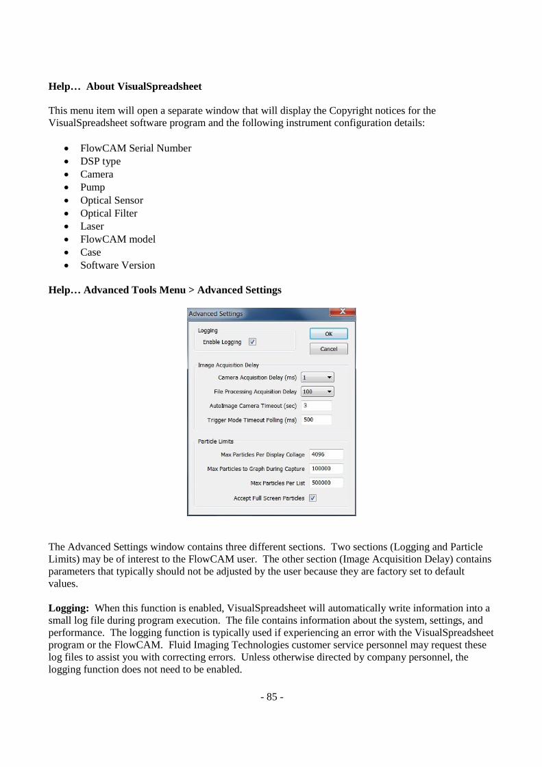
- 85 -

Help… About VisualSpreadsheet This menu item will open a separate window that will display the Copyright notices for the VisualSpreadsheet software program and the following instrument configuration details:

· FlowCAM Serial Number · DSP type · Camera · Pump · Optical Sensor · Optical Filter · Laser · FlowCAM model · Case · Software Version

Help… Advanced Tools Menu > Advanced Settings

The Advanced Settings window contains three different sections. Two sections (Logging and Particle Limits) may be of interest to the FlowCAM user. The other section (Image Acquisition Delay) contains parameters that typically should not be adjusted by the user because they are factory set to default values. Logging: When this function is enabled, VisualSpreadsheet will automatically write information into a small log file during program execution. The file contains information about the system, settings, and performance. The logging function is typically used if experiencing an error with the VisualSpreadsheet program or the FlowCAM. Fluid Imaging Technologies customer service personnel may request these log files to assist you with correcting errors. Unless otherwise directed by company personnel, the logging function does not need to be enabled.

- 86 -

Particles Limits Max Particles Per Display Collage: This parameter value can be increased or decreased to satisfy user needs and requirements. Max Particles to Graph During Capture: This parameter value can be increased or decreased to satisfy user needs and requirements. Max Particles Per List: This parameter value can be increased or decreased to suit user needs and requirements. Accept Full Screen Particles: This check box will enable the software to capture and accept sample particles that are of a size that has them contacting one edge of the field of view to a second edge. Note that the field of view is determined by the acceptable region setting. Help… Advanced Tools Menu > Advanced Calibration Calibration Factor (microns per pixel) - The Calibration Factor is used to convert measurements made in pixels to microns. The factory determined Default Value, along with the Current Value being used, is displayed in this window. Fluid Imaging Technologies does not recommend adjusting the factory determined Calibration Factor. However, the Advanced Calibration function will allow for the use of a New Calibration Factor. If a new value is entered and the Apply button is selected, a warning will be displayed to indicate that a critical value is about to be modified. Select Yes to continue or No to cancel. Help… Advanced Tools Menu > Advanced Timing The Advanced Timing Settings button will open a new window that contains three subsections (Recovery Time, Laser Cycle Time, Camera Trigger Duration). In general, the user should not access or adjust any of these factory set parameters. Help… Advanced Tools Menu > DSP Monitor The DSP Monitor window is an advanced area that is for use by Fluid Imaging Technologies trained personnel. It is not recommended that the FlowCAM user adjust any of these values or settings unless directly instructed to do so by customer service personnel. Help… Advanced Tools Menu > Scatter Detector Monitor The Scatter Detector Monitor window is an advanced area that is for use by Fluid Imaging Technologies trained personnel. It is not recommended that the FlowCAM user adjust any of these values or settings unless directly instructed to do so by customer service personnel. Help… Advanced Tools Menu > Camera Type The Camera Type window is an advanced area that is for use by Fluid Imaging Technologies trained personnel. It is not recommended that the FlowCAM user adjust any of these values or settings unless directly instructed to do so by customer service personnel.

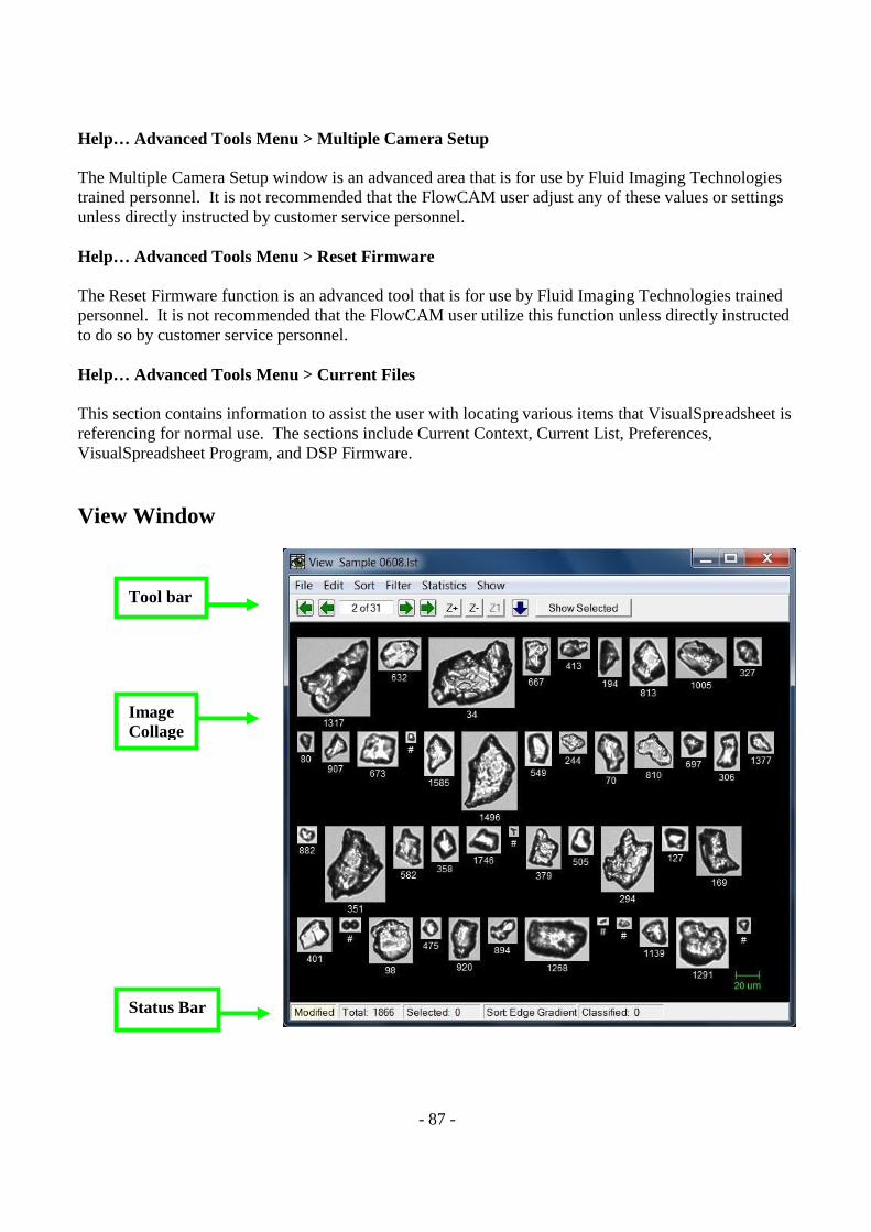
- 87 -

Help… Advanced Tools Menu > Multiple Camera Setup The Multiple Camera Setup window is an advanced area that is for use by Fluid Imaging Technologies trained personnel. It is not recommended that the FlowCAM user adjust any of these values or settings unless directly instructed by customer service personnel. Help… Advanced Tools Menu > Reset Firmware The Reset Firmware function is an advanced tool that is for use by Fluid Imaging Technologies trained personnel. It is not recommended that the FlowCAM user utilize this function unless directly instructed to do so by customer service personnel. Help… Advanced Tools Menu > Current Files This section contains information to assist the user with locating various items that VisualSpreadsheet is referencing for normal use. The sections include Current Context, Current List, Preferences, VisualSpreadsheet Program, and DSP Firmware.

View Window

Tool bar

Status Bar

Image Collage

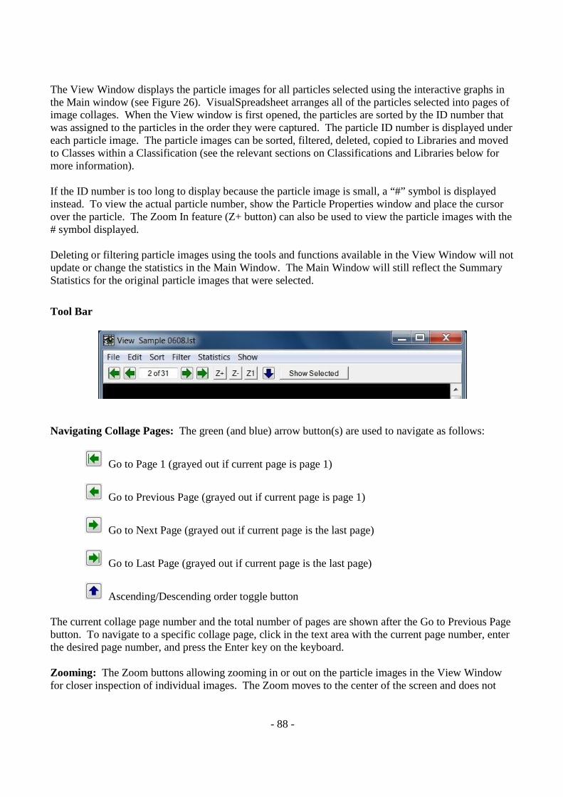
- 88 -

The View Window displays the particle images for all particles selected using the interactive graphs in the Main window (see Figure 26). VisualSpreadsheet arranges all of the particles selected into pages of image collages. When the View window is first opened, the particles are sorted by the ID number that was assigned to the particles in the order they were captured. The particle ID number is displayed under each particle image. The particle images can be sorted, filtered, deleted, copied to Libraries and moved to Classes within a Classification (see the relevant sections on Classifications and Libraries below for more information). If the ID number is too long to display because the particle image is small, a “#” symbol is displayed instead. To view the actual particle number, show the Particle Properties window and place the cursor over the particle. The Zoom In feature (Z+ button) can also be used to view the particle images with the # symbol displayed. Deleting or filtering particle images using the tools and functions available in the View Window will not update or change the statistics in the Main Window. The Main Window will still reflect the Summary Statistics for the original particle images that were selected.

Tool Bar

Navigating Collage Pages: The green (and blue) arrow button(s) are used to navigate as follows:

Go to Page 1 (grayed out if current page is page 1)

Go to Previous Page (grayed out if current page is page 1)

Go to Next Page (grayed out if current page is the last page)

Go to Last Page (grayed out if current page is the last page)

Ascending/Descending order toggle button

The current collage page number and the total number of pages are shown after the Go to Previous Page button. To navigate to a specific collage page, click in the text area with the current page number, enter the desired page number, and press the Enter key on the keyboard. Zooming: The Zoom buttons allowing zooming in or out on the particle images in the View Window for closer inspection of individual images. The Zoom moves to the center of the screen and does not

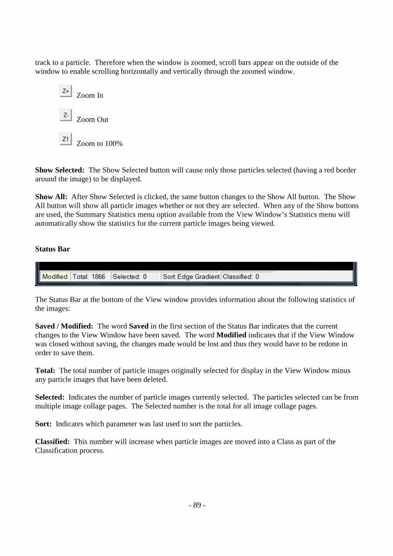
- 89 -

track to a particle. Therefore when the window is zoomed, scroll bars appear on the outside of the window to enable scrolling horizontally and vertically through the zoomed window.

Zoom In

Zoom Out

Zoom to 100%

Show Selected: The Show Selected button will cause only those particles selected (having a red border around the image) to be displayed. Show All: After Show Selected is clicked, the same button changes to the Show All button. The Show All button will show all particle images whether or not they are selected. When any of the Show buttons are used, the Summary Statistics menu option available from the View Window’s Statistics menu will automatically show the statistics for the current particle images being viewed.

Status Bar

The Status Bar at the bottom of the View window provides information about the following statistics of the images: Saved / Modified: The word Saved in the first section of the Status Bar indicates that the current changes to the View Window have been saved. The word Modified indicates that if the View Window was closed without saving, the changes made would be lost and thus they would have to be redone in order to save them. Total: The total number of particle images originally selected for display in the View Window minus any particle images that have been deleted. Selected: Indicates the number of particle images currently selected. The particles selected can be from multiple image collage pages. The Selected number is the total for all image collage pages. Sort: Indicates which parameter was last used to sort the particles. Classified: This number will increase when particle images are moved into a Class as part of the Classification process.

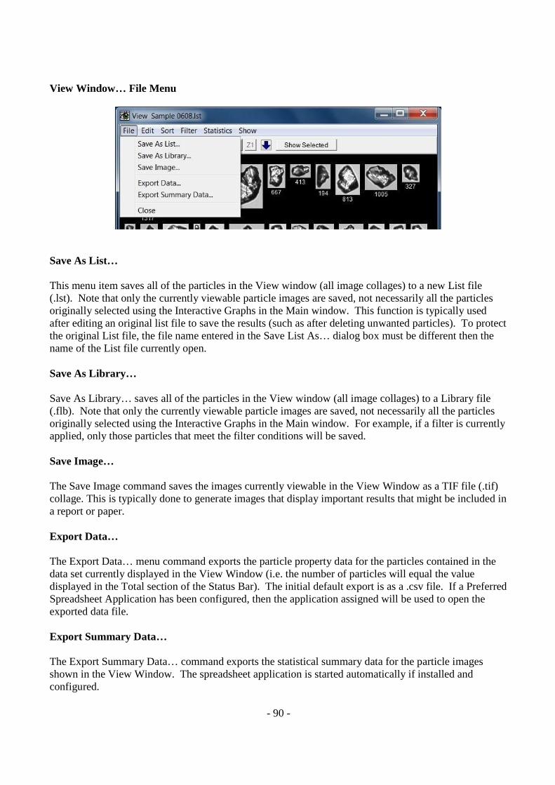
- 90 -

View Window… File Menu

Save As List… This menu item saves all of the particles in the View window (all image collages) to a new List file (.lst). Note that only the currently viewable particle images are saved, not necessarily all the particles originally selected using the Interactive Graphs in the Main window. This function is typically used after editing an original list file to save the results (such as after deleting unwanted particles). To protect the original List file, the file name entered in the Save List As… dialog box must be different then the name of the List file currently open. Save As Library… Save As Library… saves all of the particles in the View window (all image collages) to a Library file (.flb). Note that only the currently viewable particle images are saved, not necessarily all the particles originally selected using the Interactive Graphs in the Main window. For example, if a filter is currently applied, only those particles that meet the filter conditions will be saved. Save Image… The Save Image command saves the images currently viewable in the View Window as a TIF file (.tif) collage. This is typically done to generate images that display important results that might be included in a report or paper. Export Data… The Export Data… menu command exports the particle property data for the particles contained in the data set currently displayed in the View Window (i.e. the number of particles will equal the value displayed in the Total section of the Status Bar). The initial default export is as a .csv file. If a Preferred Spreadsheet Application has been configured, then the application assigned will be used to open the exported data file. Export Summary Data… The Export Summary Data… command exports the statistical summary data for the particle images shown in the View Window. The spreadsheet application is started automatically if installed and configured.

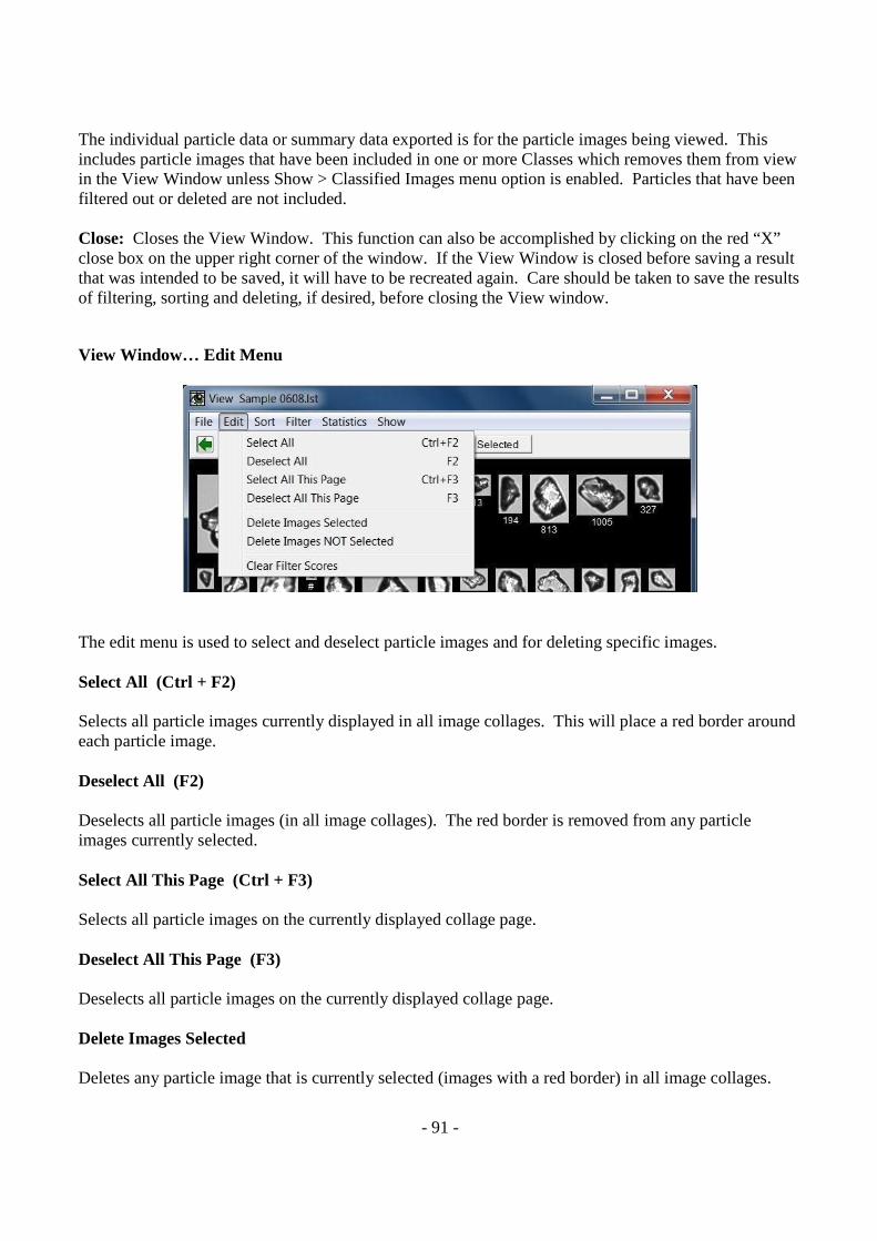
- 91 -

The individual particle data or summary data exported is for the particle images being viewed. This includes particle images that have been included in one or more Classes which removes them from view in the View Window unless Show > Classified Images menu option is enabled. Particles that have been filtered out or deleted are not included. Close: Closes the View Window. This function can also be accomplished by clicking on the red “X” close box on the upper right corner of the window. If the View Window is closed before saving a result that was intended to be saved, it will have to be recreated again. Care should be taken to save the results of filtering, sorting and deleting, if desired, before closing the View window.

View Window… Edit Menu

The edit menu is used to select and deselect particle images and for deleting specific images. Select All (Ctrl + F2) Selects all particle images currently displayed in all image collages. This will place a red border around each particle image. Deselect All (F2) Deselects all particle images (in all image collages). The red border is removed from any particle images currently selected. Select All This Page (Ctrl + F3) Selects all particle images on the currently displayed collage page. Deselect All This Page (F3) Deselects all particle images on the currently displayed collage page. Delete Images Selected Deletes any particle image that is currently selected (images with a red border) in all image collages.

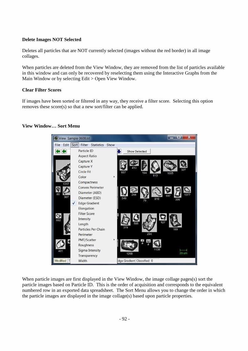
- 92 -

Delete Images NOT Selected Deletes all particles that are NOT currently selected (images without the red border) in all image collages. When particles are deleted from the View Window, they are removed from the list of particles available in this window and can only be recovered by reselecting them using the Interactive Graphs from the Main Window or by selecting Edit > Open View Window. Clear Filter Scores If images have been sorted or filtered in any way, they receive a filter score. Selecting this option removes these score(s) so that a new sort/filter can be applied.

View Window… Sort Menu

When particle images are first displayed in the View Window, the image collage pages(s) sort the particle images based on Particle ID. This is the order of acquisition and corresponds to the equivalent numbered row in an exported data spreadsheet. The Sort Menu allows you to change the order in which the particle images are displayed in the image collage(s) based upon particle properties.

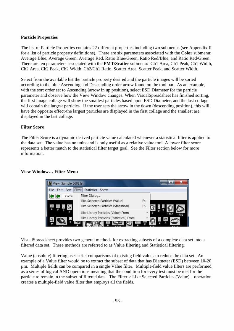
- 93 -

Particle Properties The list of Particle Properties contains 22 different properties including two submenus (see Appendix II for a list of particle property definitions). There are six parameters associated with the Color submenu: Average Blue, Average Green, Average Red, Ratio Blue/Green, Ratio Red/Blue, and Ratio Red/Green. There are ten parameters associated with the PMT/Scatter submenu: Ch1 Area, Ch1 Peak, Ch1 Width, Ch2 Area, Ch2 Peak, Ch2 Width, Ch2/Ch1 Ratio, Scatter Area, Scatter Peak, and Scatter Width. Select from the available list the particle property desired and the particle images will be sorted according to the blue Ascending and Descending order arrow found on the tool bar. As an example, with the sort order set to Ascending (arrow in up position), select ESD Diameter for the particle parameter and observe how the View Window changes. When VisualSpreadsheet has finished sorting, the first image collage will show the smallest particles based upon ESD Diameter, and the last collage will contain the largest particles. If the user sets the arrow in the down (descending position), this will have the opposite effect-the largest particles are displayed in the first collage and the smallest are displayed in the last collage. Filter Score The Filter Score is a dynamic derived particle value calculated whenever a statistical filter is applied to the data set. The value has no units and is only useful as a relative value tool. A lower filter score represents a better match to the statistical filter target goal. See the Filter section below for more information.

View Window… Filter Menu

VisualSpreadsheet provides two general methods for extracting subsets of a complete data set into a filtered data set. These methods are referred to as Value filtering and Statistical filtering. Value (absolute) filtering uses strict comparisons of existing field values to reduce the data set. An example of a Value filter would be to extract the subset of data that has Diameter (ESD) between 10-20 µm. Multiple fields can be compared in a single Value filter. Multiple-field value filters are performed as a series of logical AND operations meaning that the condition for every test must be met for the particle to remain in the subset of filtered data. The Filter > Like Selected Particles (Value)... operation creates a multiple-field value filter that employs all the fields.

- 94 -

The other type of filtering (relative) used by VisualSpreadsheet is called Statistical filtering. Statistical filtering uses a simple procedure where the user provides a representative training set of particles and VisualSpreadsheet uses this set to generalize an ideal target particle. This target particle is then compared against the entire data set and each particle is scored based on their ‘likeness’ or similarity to the target. Unlike the value filter which is strictly a boolean test for inclusion in a data subset, statistical filtering can only rank the particles based on their ‘likeness’ to the target. The value for this likeness is dynamically recorded for each particle as the Filter Score field. A particle's Filter Score is always a transient value, recalculated whenever a statistical filtering operation is run against the particle. It has no units and is not stored on disk. Filter scores lend themselves to sorting or ranking particles and so the Filter Score field is available as a Sorting field. The default behavior of an interactive statistical filter operation is to sort the particles in ascending Filter Score order. A statistical filter by itself cannot generate a subset of the data. To generate a subset, a cutoff value is needed to use with the Filter Score to partition the data into two subsets, particles like those in the training set and particles not like those in the training set. A natural choice for the cutoff value is the Filter Score of the highest scoring particle in the user-provided training set. This is the default value that VisualSpreadsheet uses for this situation. Filter Score values that are less then or equal to the highest scoring particle in the training set are considered ‘like’ the target, those with higher Filter Scores are considered ‘unlike’. The cutoff value is simply a value filter applied after the statistical filter has been run and its value can be manually adjusted in the filter dialog. Filter Dialog… The Filter Dialog is a tool that allows the user to build filters based on parameter measurements (value) or derived statistics (statistical). The Filter Dialog can be utilized at acquisition or during post-run analysis from the following locations (in addition to using the View Window > Filter > Filter Dialog… pathway described in this section):

· Main Window > Setup > Context > Filter (tab) > Advanced Acquisition Filter (section). Using a single filter at this location allows the user to select and define which particles are going to be captured and placed into the collage window during an analysis.

· Main Window > Preferences > Main Window Settings > Filter Grid (tab) > Filters (section).

Using one or more filters at this location allows the user to automatically bin particles at the time of acquisition. These filters can be displayed in the Main Window Filter Grid, with selected statistics.

· Main Window > Open Library or Open Classification Window. The use of the Filter Dialog in

these windows is described in the Library and Classification sections.

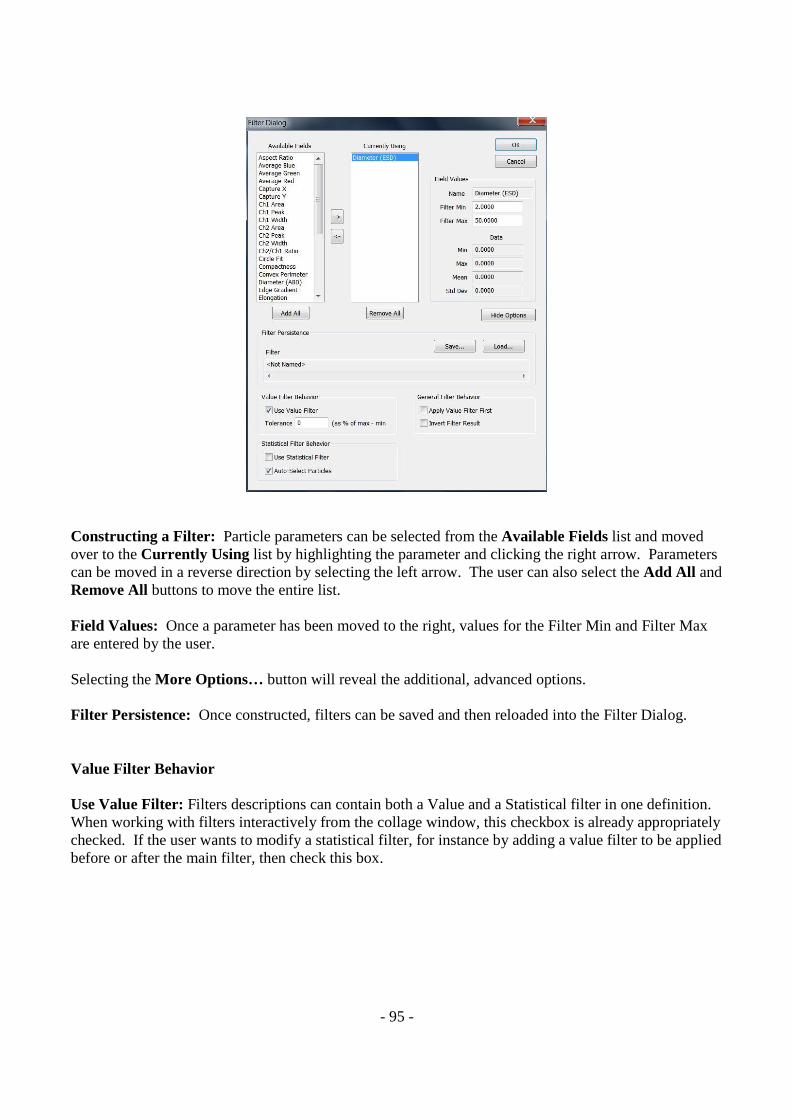
- 95 -

Constructing a Filter: Particle parameters can be selected from the Available Fields list and moved over to the Currently Using list by highlighting the parameter and clicking the right arrow. Parameters can be moved in a reverse direction by selecting the left arrow. The user can also select the Add All and Remove All buttons to move the entire list. Field Values: Once a parameter has been moved to the right, values for the Filter Min and Filter Max are entered by the user. Selecting the More Options… button will reveal the additional, advanced options. Filter Persistence: Once constructed, filters can be saved and then reloaded into the Filter Dialog. Value Filter Behavior Use Value Filter: Filters descriptions can contain both a Value and a Statistical filter in one definition. When working with filters interactively from the collage window, this checkbox is already appropriately checked. If the user wants to modify a statistical filter, for instance by adding a value filter to be applied before or after the main filter, then check this box.

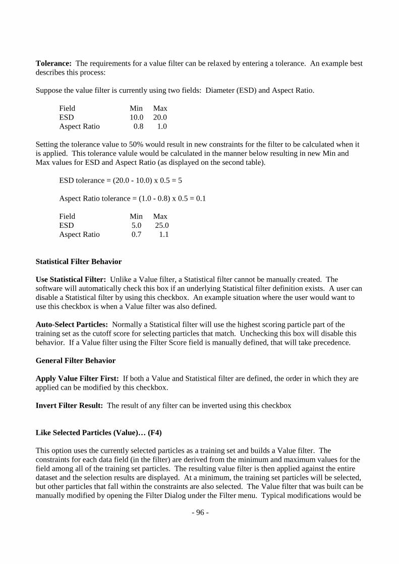
- 96 -

Tolerance: The requirements for a value filter can be relaxed by entering a tolerance. An example best describes this process: Suppose the value filter is currently using two fields: Diameter (ESD) and Aspect Ratio. Field Min Max ESD 10.0 20.0 Aspect Ratio 0.8 1.0 Setting the tolerance value to 50% would result in new constraints for the filter to be calculated when it is applied. This tolerance valule would be calculated in the manner below resulting in new Min and Max values for ESD and Aspect Ratio (as displayed on the second table). ESD tolerance = (20.0 - 10.0) x 0.5 = 5 Aspect Ratio tolerance = (1.0 - 0.8) x 0.5 = 0.1 Field Min Max ESD 5.0 25.0 Aspect Ratio 0.7 1.1 Statistical Filter Behavior Use Statistical Filter: Unlike a Value filter, a Statistical filter cannot be manually created. The software will automatically check this box if an underlying Statistical filter definition exists. A user can disable a Statistical filter by using this checkbox. An example situation where the user would want to use this checkbox is when a Value filter was also defined. Auto-Select Particles: Normally a Statistical filter will use the highest scoring particle part of the training set as the cutoff score for selecting particles that match. Unchecking this box will disable this behavior. If a Value filter using the Filter Score field is manually defined, that will take precedence. General Filter Behavior Apply Value Filter First: If both a Value and Statistical filter are defined, the order in which they are applied can be modified by this checkbox. Invert Filter Result: The result of any filter can be inverted using this checkbox Like Selected Particles (Value)… (F4) This option uses the currently selected particles as a training set and builds a Value filter. The constraints for each data field (in the filter) are derived from the minimum and maximum values for the field among all of the training set particles. The resulting value filter is then applied against the entire dataset and the selection results are displayed. At a minimum, the training set particles will be selected, but other particles that fall within the constraints are also selected. The Value filter that was built can be manually modified by opening the Filter Dialog under the Filter menu. Typical modifications would be

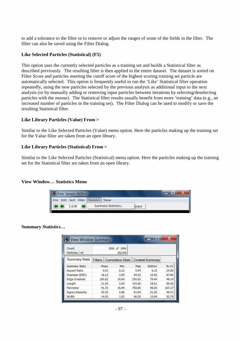
- 97 -

to add a tolerance to the filter or to remove or adjust the ranges of some of the fields in the filter. The filter can also be saved using the Filter Dialog. Like Selected Particles (Statistical) (F5) This option uses the currently selected particles as a training set and builds a Statistical filter as described previously. The resulting filter is then applied to the entire dataset. The dataset is sorted on Filter Score and particles meeting the cutoff score of the highest scoring training set particle are automatically selected. This option is frequently useful to run the ‘Like’ Statistical filter operation repeatedly, using the new particles selected by the previous analysis as additional input to the next analysis (or by manually adding or removing input particles between iterations by selecting/deselecting particles with the mouse). The Statistical filter results usually benefit from more ‘training’ data (e.g., an increased number of particles in the training set). The Filter Dialog can be used to modify or save the resulting Statistical filter. Like Library Particles (Value) From > Similar to the Like Selected Particles (Value) menu option. Here the particles making up the training set for the Value filter are taken from an open library. Like Library Particles (Statistical) From > Similar to the Like Selected Particles (Statistical) menu option. Here the particles making up the training set for the Statistical filter are taken from an open library.

View Window… Statistics Menu

Summary Statistics…

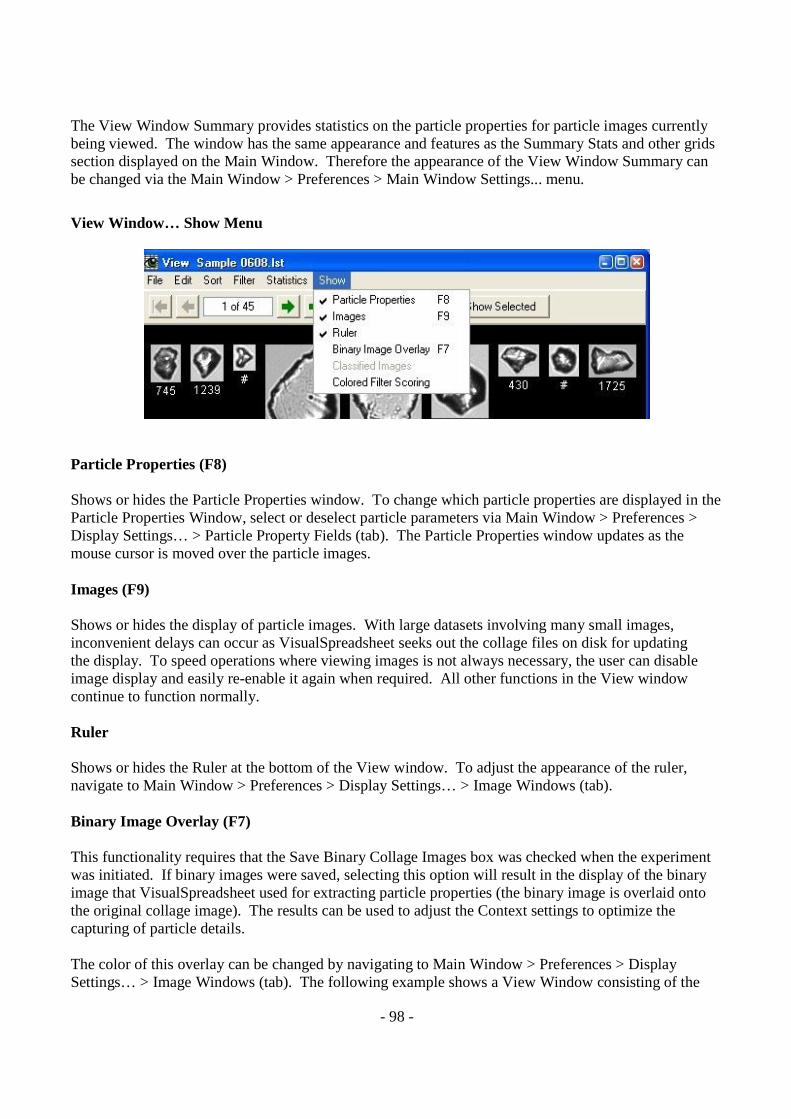
- 98 -

The View Window Summary provides statistics on the particle properties for particle images currently being viewed. The window has the same appearance and features as the Summary Stats and other grids section displayed on the Main Window. Therefore the appearance of the View Window Summary can be changed via the Main Window > Preferences > Main Window Settings... menu.

View Window… Show Menu

Particle Properties (F8) Shows or hides the Particle Properties window. To change which particle properties are displayed in the Particle Properties Window, select or deselect particle parameters via Main Window > Preferences > Display Settings… > Particle Property Fields (tab). The Particle Properties window updates as the mouse cursor is moved over the particle images. Images (F9)

Shows or hides the display of particle images. With large datasets involving many small images, inconvenient delays can occur as VisualSpreadsheet seeks out the collage files on disk for updating the display. To speed operations where viewing images is not always necessary, the user can disable image display and easily re-enable it again when required. All other functions in the View window continue to function normally. Ruler Shows or hides the Ruler at the bottom of the View window. To adjust the appearance of the ruler, navigate to Main Window > Preferences > Display Settings… > Image Windows (tab). Binary Image Overlay (F7) This functionality requires that the Save Binary Collage Images box was checked when the experiment was initiated. If binary images were saved, selecting this option will result in the display of the binary image that VisualSpreadsheet used for extracting particle properties (the binary image is overlaid onto the original collage image). The results can be used to adjust the Context settings to optimize the capturing of particle details. The color of this overlay can be changed by navigating to Main Window > Preferences > Display Settings… > Image Windows (tab). The following example shows a View Window consisting of the

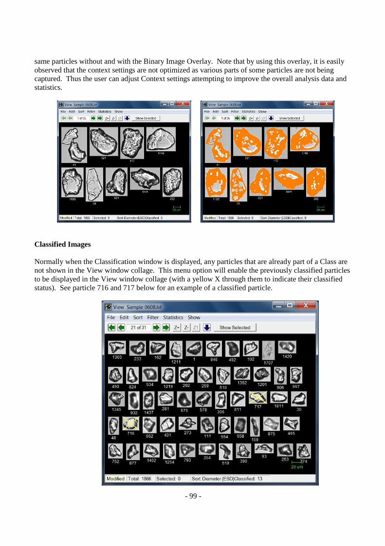
- 99 -

same particles without and with the Binary Image Overlay. Note that by using this overlay, it is easily observed that the context settings are not optimized as various parts of some particles are not being captured. Thus the user can adjust Context settings attempting to improve the overall analysis data and statistics.

Classified Images Normally when the Classification window is displayed, any particles that are already part of a Class are not shown in the View window collage. This menu option will enable the previously classified particles to be displayed in the View window collage (with a yellow X through them to indicate their classified status). See particle 716 and 717 below for an example of a classified particle.

- 100 -

Colored Filter Scoring Colored Filter Scoring is used in conjunction with Show Particles Properties. After filtering particles in the View Window (via the functions in the Filter menu), selecting this function allows the user to see why particles were or were not sorted together by the use of various shades of colors. If parameters (as seen in the Particle Properties window) are lightly colored, then their differences from filtering values were minimal; if they are darkly colored, then their differences from filtering values were significant, explaining why the particles were not sorted near the top of the list.

Right Click Popup Menu To use the Rick Click Popup Menu in the View Window, right click on one of the particle images. The following three options become available for selection: Delete Particle: Removes the particle image from the View Window and resets to Page One of the open View Window. The particle image is still available through reselection using the interactive graphs in the Main Window. Add To Library: Adds the particle to any Library currently open. Note that the Library Window must be open with at least one Library open in it. The particles remain selected and if this function is used again (without deselecting the particles) the same particles will be added to the Library a second time. Add To Class: Adds the particle to an open Class within the currently open Classification. Note the Classification window must be open with at least one Class open in it.

Keyboard Commands Selecting Multiple Particle Images: To select a group of particle images within the View Window, press and hold the Ctrl key, click to the left of the first particle of interest, hold down on the mouse button and drag across the remaining particle(s) of interest. User Controlled Ruler: Within the View Window, press and hold the Shift key. Left click to display a small cross on the Image Collage area. While holding, left click a second time to display a second small cross. The software will automatically display a line and the length of the line (in microns) between the two points. This function will allow the user to measure specific portions of a particle. To remove this ruler, click somewhere outside of the currently displayed ruler (to create a new cross) and then release the Shift key.

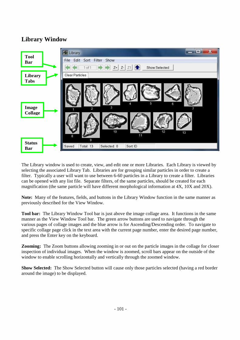
- 101 -

Library Window

The Library window is used to create, view, and edit one or more Libraries. Each Library is viewed by selecting the associated Library Tab. Libraries are for grouping similar particles in order to create a filter. Typically a user will want to use between 6-60 particles in a Library to create a filter. Libraries can be opened with any list file. Separate filters, of the same particles, should be created for each magnification (the same particle will have different morphological information at 4X, 10X and 20X). Note: Many of the features, fields, and buttons in the Library Window function in the same manner as previously described for the View Window. Tool bar: The Library Window Tool bar is just above the image collage area. It functions in the same manner as the View Window Tool bar. The green arrow buttons are used to navigate through the various pages of collage images and the blue arrow is for Ascending/Descending order. To navigate to specific collage page click in the text area with the current page number, enter the desired page number, and press the Enter key on the keyboard. Zooming: The Zoom buttons allowing zooming in or out on the particle images in the collage for closer inspection of individual images. When the window is zoomed, scroll bars appear on the outside of the window to enable scrolling horizontally and vertically through the zoomed window. Show Selected: The Show Selected button will cause only those particles selected (having a red border around the image) to be displayed.

Tool Bar

Library Tabs

Image Collage

Status Bar

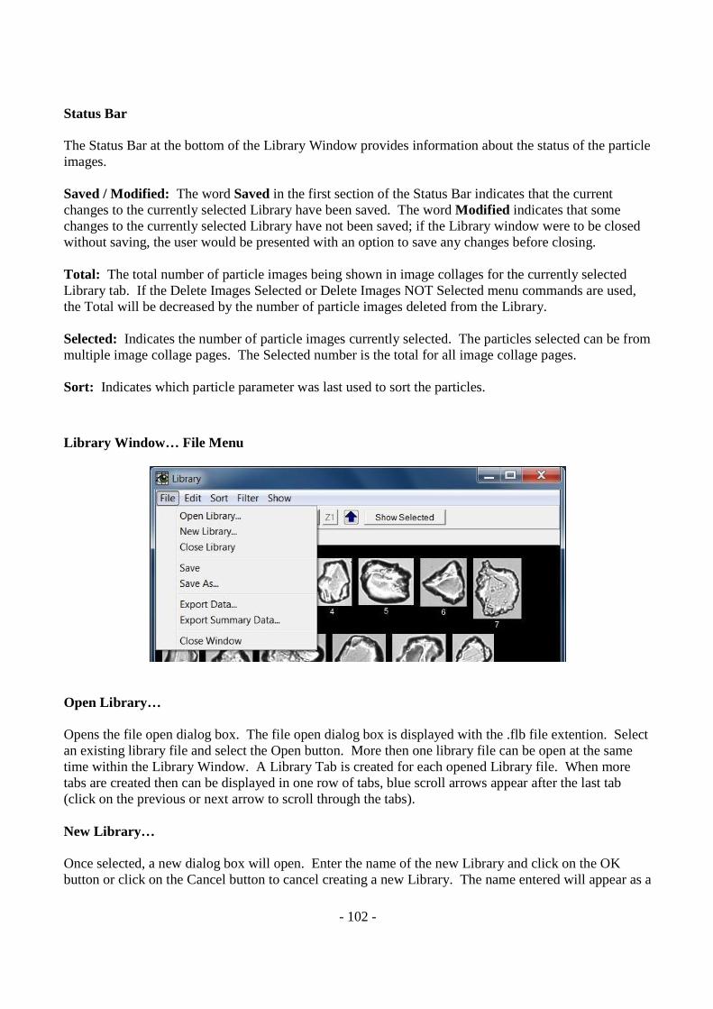
- 102 -

Status Bar The Status Bar at the bottom of the Library Window provides information about the status of the particle images. Saved / Modified: The word Saved in the first section of the Status Bar indicates that the current changes to the currently selected Library have been saved. The word Modified indicates that some changes to the currently selected Library have not been saved; if the Library window were to be closed without saving, the user would be presented with an option to save any changes before closing. Total: The total number of particle images being shown in image collages for the currently selected Library tab. If the Delete Images Selected or Delete Images NOT Selected menu commands are used, the Total will be decreased by the number of particle images deleted from the Library. Selected: Indicates the number of particle images currently selected. The particles selected can be from multiple image collage pages. The Selected number is the total for all image collage pages. Sort: Indicates which particle parameter was last used to sort the particles.

Library Window… File Menu

Open Library… Opens the file open dialog box. The file open dialog box is displayed with the .flb file extention. Select an existing library file and select the Open button. More then one library file can be open at the same time within the Library Window. A Library Tab is created for each opened Library file. When more tabs are created then can be displayed in one row of tabs, blue scroll arrows appear after the last tab (click on the previous or next arrow to scroll through the tabs). New Library… Once selected, a new dialog box will open. Enter the name of the new Library and click on the OK button or click on the Cancel button to cancel creating a new Library. The name entered will appear as a

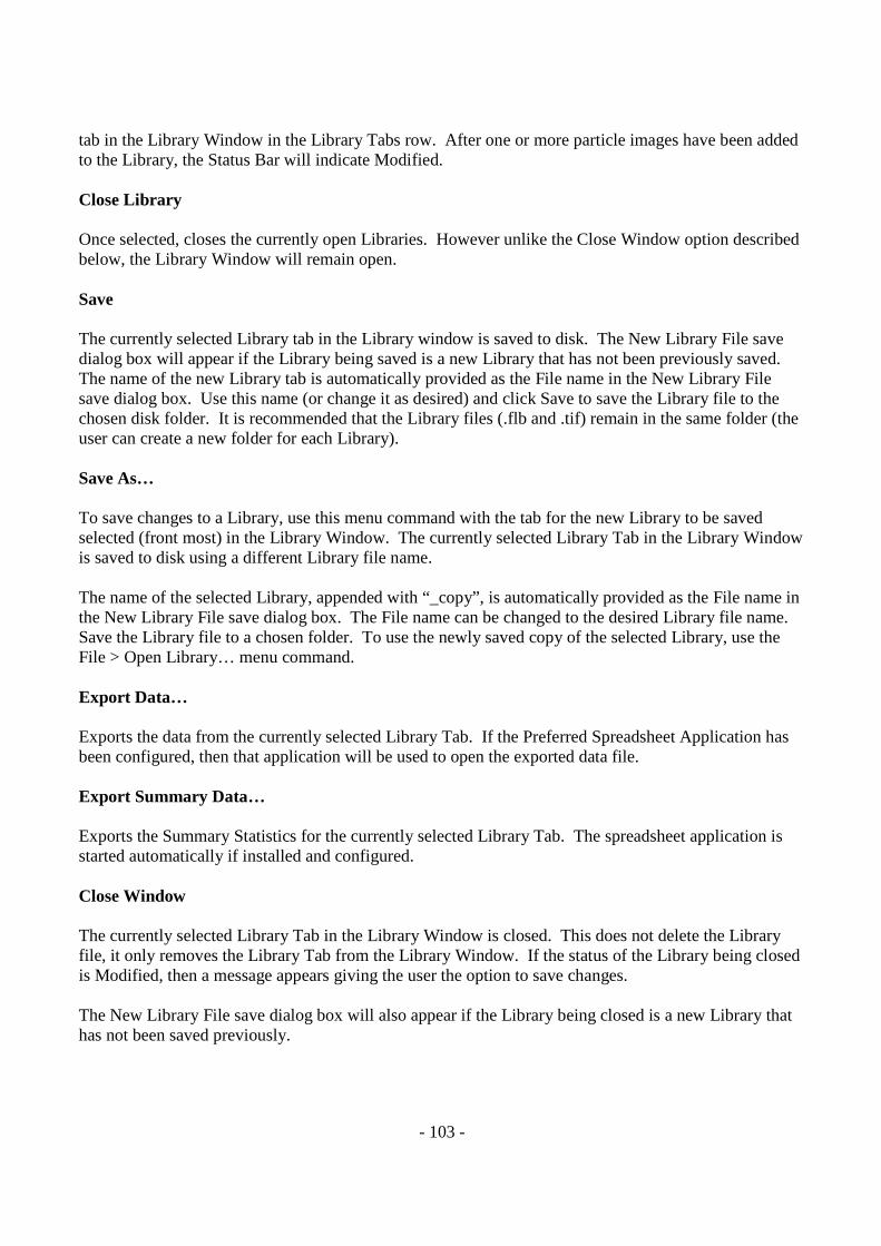
- 103 -

tab in the Library Window in the Library Tabs row. After one or more particle images have been added to the Library, the Status Bar will indicate Modified. Close Library Once selected, closes the currently open Libraries. However unlike the Close Window option described below, the Library Window will remain open. Save The currently selected Library tab in the Library window is saved to disk. The New Library File save dialog box will appear if the Library being saved is a new Library that has not been previously saved. The name of the new Library tab is automatically provided as the File name in the New Library File save dialog box. Use this name (or change it as desired) and click Save to save the Library file to the chosen disk folder. It is recommended that the Library files (.flb and .tif) remain in the same folder (the user can create a new folder for each Library). Save As… To save changes to a Library, use this menu command with the tab for the new Library to be saved selected (front most) in the Library Window. The currently selected Library Tab in the Library Window is saved to disk using a different Library file name. The name of the selected Library, appended with “_copy”, is automatically provided as the File name in the New Library File save dialog box. The File name can be changed to the desired Library file name. Save the Library file to a chosen folder. To use the newly saved copy of the selected Library, use the File > Open Library… menu command. Export Data… Exports the data from the currently selected Library Tab. If the Preferred Spreadsheet Application has been configured, then that application will be used to open the exported data file. Export Summary Data… Exports the Summary Statistics for the currently selected Library Tab. The spreadsheet application is started automatically if installed and configured. Close Window The currently selected Library Tab in the Library Window is closed. This does not delete the Library file, it only removes the Library Tab from the Library Window. If the status of the Library being closed is Modified, then a message appears giving the user the option to save changes. The New Library File save dialog box will also appear if the Library being closed is a new Library that has not been saved previously.

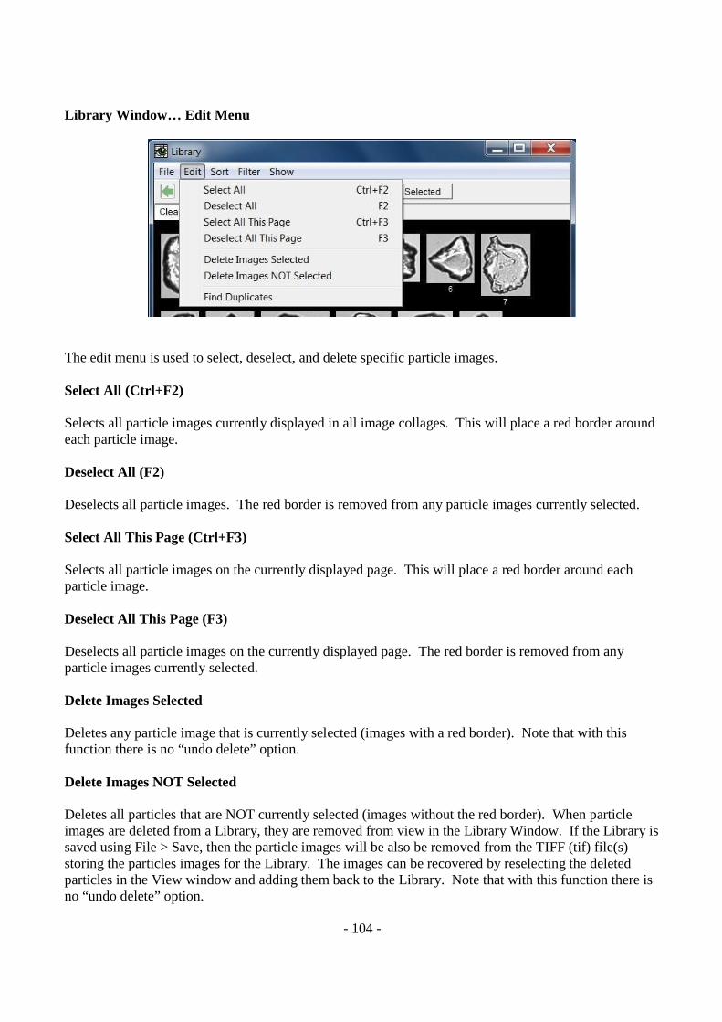
- 104 -

Library Window… Edit Menu

The edit menu is used to select, deselect, and delete specific particle images. Select All (Ctrl+F2) Selects all particle images currently displayed in all image collages. This will place a red border around each particle image.

Deselect All (F2) Deselects all particle images. The red border is removed from any particle images currently selected. Select All This Page (Ctrl+F3) Selects all particle images on the currently displayed page. This will place a red border around each particle image. Deselect All This Page (F3) Deselects all particle images on the currently displayed page. The red border is removed from any particle images currently selected. Delete Images Selected Deletes any particle image that is currently selected (images with a red border). Note that with this function there is no “undo delete” option. Delete Images NOT Selected Deletes all particles that are NOT currently selected (images without the red border). When particle images are deleted from a Library, they are removed from view in the Library Window. If the Library is saved using File > Save, then the particle images will be also be removed from the TIFF (tif) file(s) storing the particles images for the Library. The images can be recovered by reselecting the deleted particles in the View window and adding them back to the Library. Note that with this function there is no “undo delete” option.

- 105 -

Find Duplicates When working with a large number of particle images and files, it is possible to erroneously add the same particles to a Library more than once. Find Duplicates searches for duplicate particle images. If any are found, the duplicate images are selected and only the selected particles are shown. To delete the duplicate images, use the Edit > Delete Images Selected menu command and then click on the Show Selected button. If no duplicate particle images are found, a message will appear indicating none were found. Once this Find Duplicates function has been utilized, the Particle ID numbers under the images will no longer be in sequential order.

Library Window… Sort Menu The Sort Menu in the Classification Window functions in the exact same manner as the Sort Menu in the View Window. When particle images are first displayed in the View window the image collage pages(s) sort the particle images based on Particle ID. This is the order of acquisition and corresponds to the equivalent numbered row in an exported data spreadsheet. The Sort Menu allows you to change the order in which the particle images are displayed in the image collage(s) based upon particle properties. Library Window… Filter Menu

Build Value Filter… Selecting this function will open a Filter dialog box and automatically populate the Currently Using section with all available fields and their corresponding values. These values are derived from the Library Tab that is highlighted. This menu item allows the user to build a filter using the particle properties/characteristics of a Library. This is a value filter (a filter based on parameter measurements). Build Statistical Filter… Selecting this function will open a Filter dialog box and automatically populate the Currently Using section with all available fields and their corresponding values. These values are derived from the Library Tab that is highlighted. This menu item allows the user to build a filter using the particle properties/characteristics of a Library. This is a statistical filter (a filter based on derived statistics).

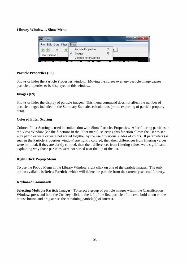
- 106 -

Library Window… Show Menu

Particle Properties (F8) Shows or hides the Particle Properties window. Moving the cursor over any particle image causes particle properties to be displayed in this window. Images (F9) Shows or hides the display of particle images. This menu command does not affect the number of particle images included in the Summary Statistics calculations (or the exporting of particle property data). Colored Filter Scoring Colored Filter Scoring is used in conjunction with Show Particles Properties. After filtering particles in the View Window (via the functions in the Filter menu), selecting this function allows the user to see why particles were or were not sorted together by the use of various shades of colors. If parameters (as seen in the Particle Properties window) are lightly colored, then their differences from filtering values were minimal; if they are darkly colored, then their differences from filtering values were significant, explaining why those particles were not sorted near the top of the list.

Right Click Popup Menu To use the Popup Menu in the Library Window, right click on one of the particle images. The only option available is Delete Particle, which will delete the particle from the currently selected Library.

Keyboard Commands Selecting Multiple Particle Images: To select a group of particle images within the Classification Window, press and hold the Ctrl key, click to the left of the first particle of interest, hold down on the mouse button and drag across the remaining particle(s) of interest.

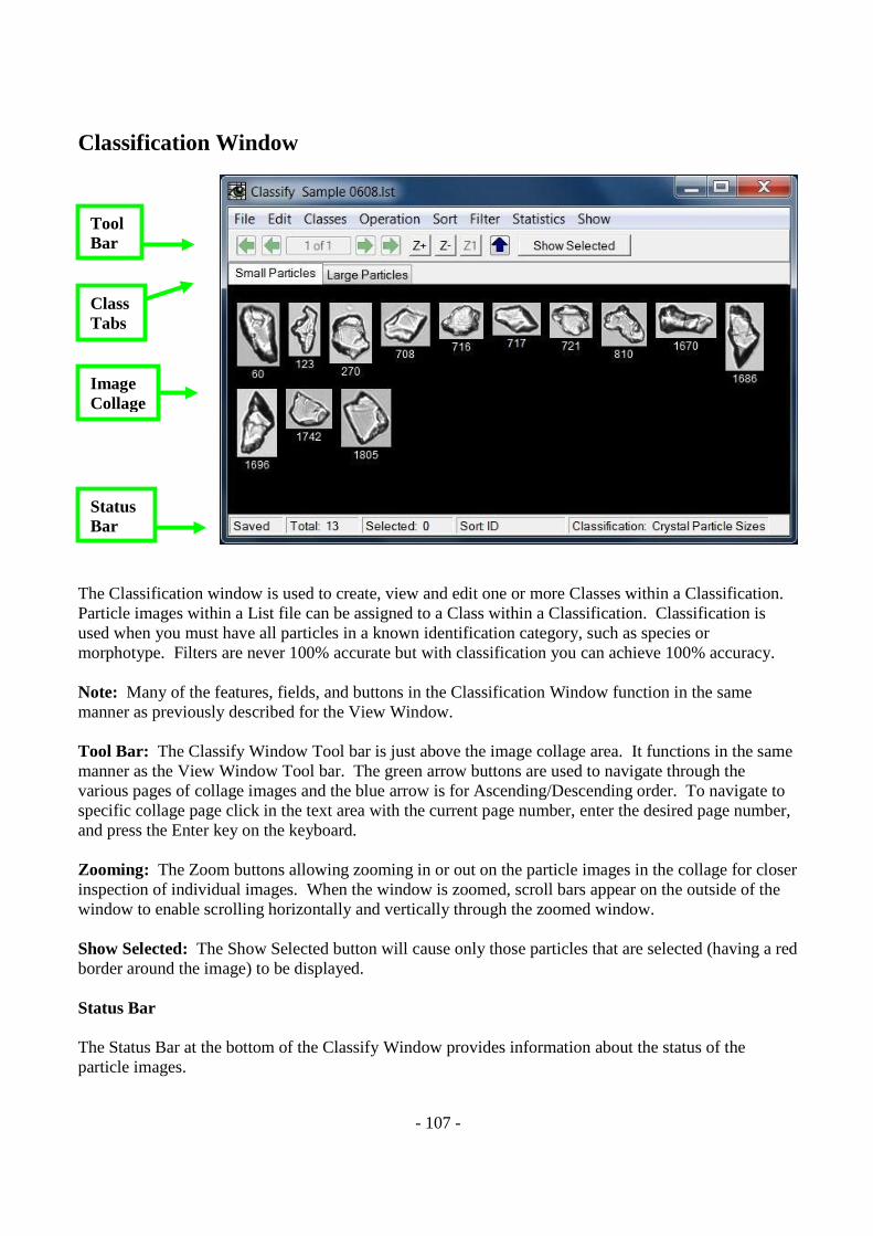
- 107 -

Classification Window

The Classification window is used to create, view and edit one or more Classes within a Classification. Particle images within a List file can be assigned to a Class within a Classification. Classification is used when you must have all particles in a known identification category, such as species or morphotype. Filters are never 100% accurate but with classification you can achieve 100% accuracy. Note: Many of the features, fields, and buttons in the Classification Window function in the same manner as previously described for the View Window. Tool Bar: The Classify Window Tool bar is just above the image collage area. It functions in the same manner as the View Window Tool bar. The green arrow buttons are used to navigate through the various pages of collage images and the blue arrow is for Ascending/Descending order. To navigate to specific collage page click in the text area with the current page number, enter the desired page number, and press the Enter key on the keyboard. Zooming: The Zoom buttons allowing zooming in or out on the particle images in the collage for closer inspection of individual images. When the window is zoomed, scroll bars appear on the outside of the window to enable scrolling horizontally and vertically through the zoomed window. Show Selected: The Show Selected button will cause only those particles that are selected (having a red border around the image) to be displayed. Status Bar The Status Bar at the bottom of the Classify Window provides information about the status of the particle images.

Tool Bar

Class Tabs

Image Collage

Status Bar

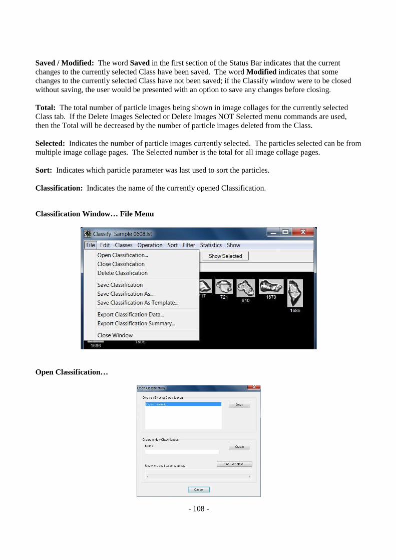
- 108 -

Saved / Modified: The word Saved in the first section of the Status Bar indicates that the current changes to the currently selected Class have been saved. The word Modified indicates that some changes to the currently selected Class have not been saved; if the Classify window were to be closed without saving, the user would be presented with an option to save any changes before closing. Total: The total number of particle images being shown in image collages for the currently selected Class tab. If the Delete Images Selected or Delete Images NOT Selected menu commands are used, then the Total will be decreased by the number of particle images deleted from the Class. Selected: Indicates the number of particle images currently selected. The particles selected can be from multiple image collage pages. The Selected number is the total for all image collage pages. Sort: Indicates which particle parameter was last used to sort the particles. Classification: Indicates the name of the currently opened Classification.

Classification Window… File Menu

Open Classification…

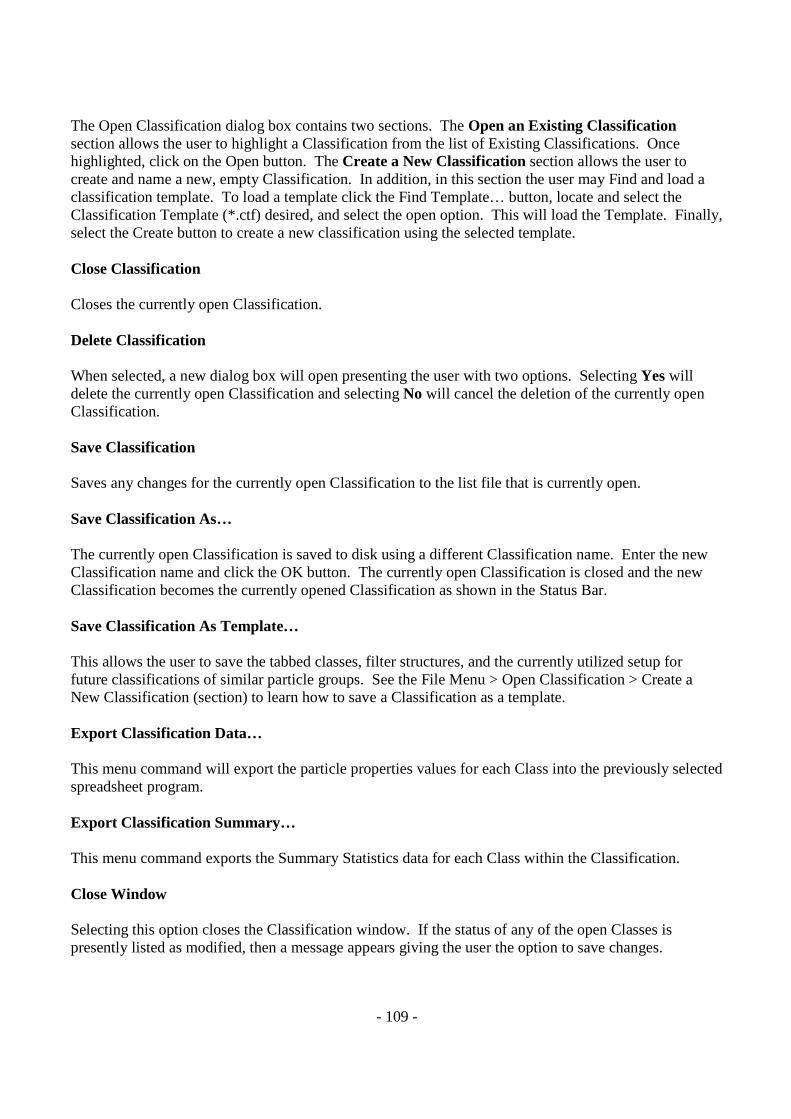
- 109 -

The Open Classification dialog box contains two sections. The Open an Existing Classification section allows the user to highlight a Classification from the list of Existing Classifications. Once highlighted, click on the Open button. The Create a New Classification section allows the user to create and name a new, empty Classification. In addition, in this section the user may Find and load a classification template. To load a template click the Find Template… button, locate and select the Classification Template (*.ctf) desired, and select the open option. This will load the Template. Finally, select the Create button to create a new classification using the selected template. Close Classification Closes the currently open Classification. Delete Classification When selected, a new dialog box will open presenting the user with two options. Selecting Yes will delete the currently open Classification and selecting No will cancel the deletion of the currently open Classification. Save Classification Saves any changes for the currently open Classification to the list file that is currently open. Save Classification As… The currently open Classification is saved to disk using a different Classification name. Enter the new Classification name and click the OK button. The currently open Classification is closed and the new Classification becomes the currently opened Classification as shown in the Status Bar. Save Classification As Template… This allows the user to save the tabbed classes, filter structures, and the currently utilized setup for future classifications of similar particle groups. See the File Menu > Open Classification > Create a New Classification (section) to learn how to save a Classification as a template. Export Classification Data… This menu command will export the particle properties values for each Class into the previously selected spreadsheet program. Export Classification Summary… This menu command exports the Summary Statistics data for each Class within the Classification. Close Window Selecting this option closes the Classification window. If the status of any of the open Classes is presently listed as modified, then a message appears giving the user the option to save changes.

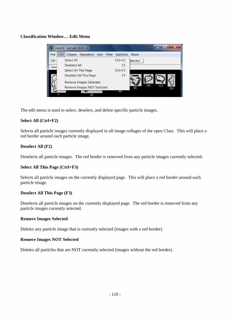
- 110 -

Classification Window… Edit Menu

The edit menu is used to select, deselect, and delete specific particle images. Select All (Ctrl+F2) Selects all particle images currently displayed in all image collages of the open Class. This will place a red border around each particle image.

Deselect All (F2) Deselects all particle images. The red border is removed from any particle images currently selected. Select All This Page (Ctrl+F3) Selects all particle images on the currently displayed page. This will place a red border around each particle image. Deselect All This Page (F3) Deselects all particle images on the currently displayed page. The red border is removed from any particle images currently selected. Remove Images Selected Deletes any particle image that is currently selected (images with a red border). Remove Images NOT Selected Deletes all particles that are NOT currently selected (images without the red border).

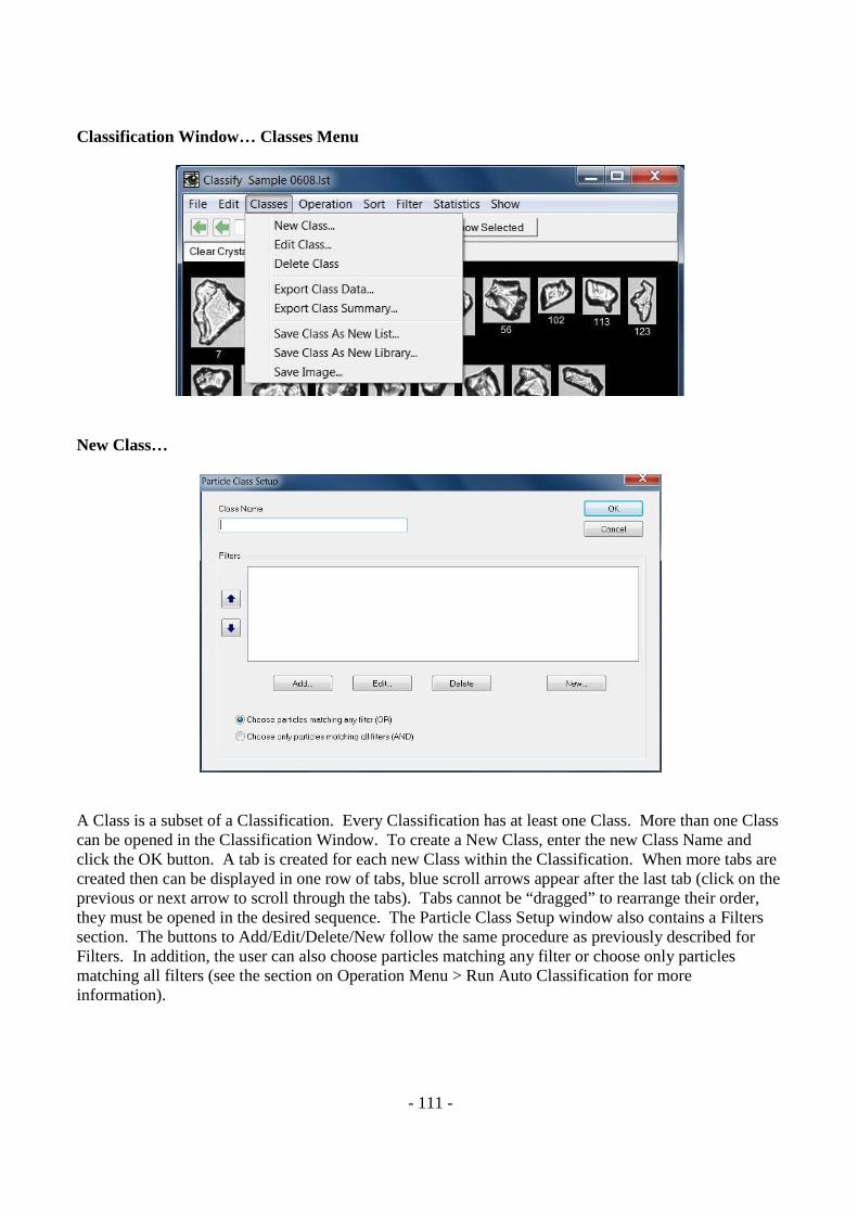
- 111 -

Classification Window… Classes Menu

New Class…

A Class is a subset of a Classification. Every Classification has at least one Class. More than one Class can be opened in the Classification Window. To create a New Class, enter the new Class Name and click the OK button. A tab is created for each new Class within the Classification. When more tabs are created then can be displayed in one row of tabs, blue scroll arrows appear after the last tab (click on the previous or next arrow to scroll through the tabs). Tabs cannot be “dragged” to rearrange their order, they must be opened in the desired sequence. The Particle Class Setup window also contains a Filters section. The buttons to Add/Edit/Delete/New follow the same procedure as previously described for Filters. In addition, the user can also choose particles matching any filter or choose only particles matching all filters (see the section on Operation Menu > Run Auto Classification for more information).

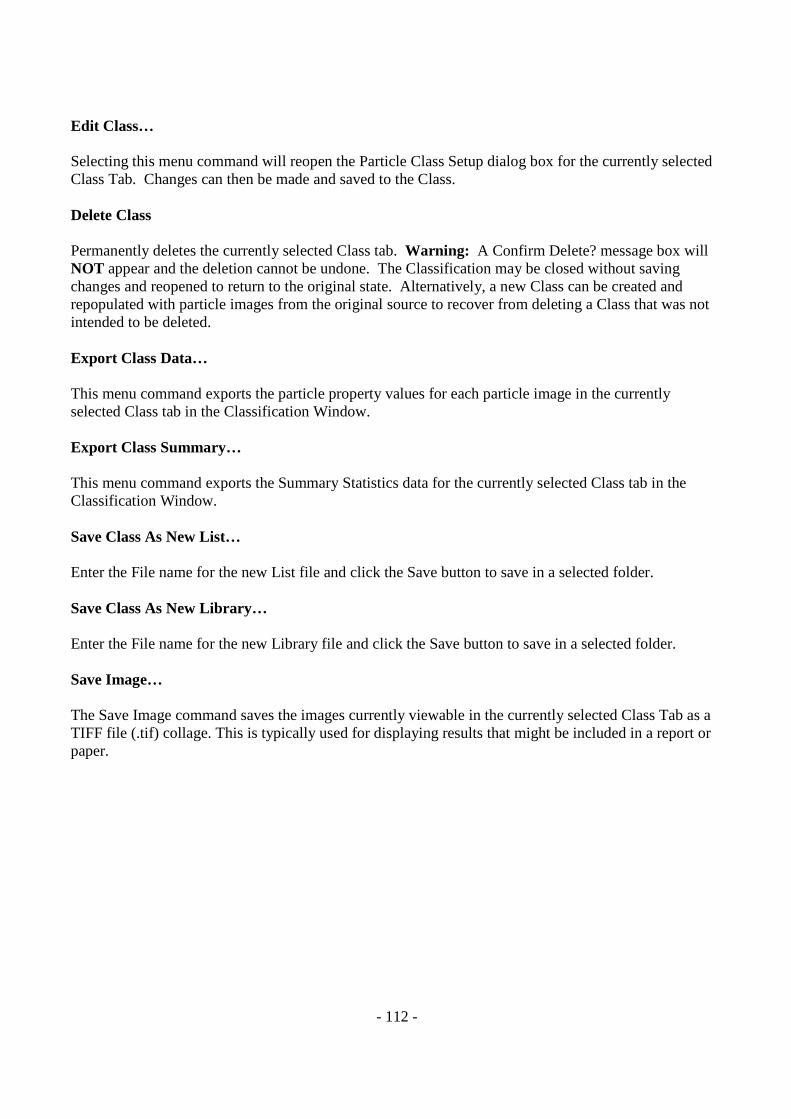
- 112 -

Edit Class… Selecting this menu command will reopen the Particle Class Setup dialog box for the currently selected Class Tab. Changes can then be made and saved to the Class. Delete Class Permanently deletes the currently selected Class tab. Warning: A Confirm Delete? message box will NOT appear and the deletion cannot be undone. The Classification may be closed without saving changes and reopened to return to the original state. Alternatively, a new Class can be created and repopulated with particle images from the original source to recover from deleting a Class that was not intended to be deleted. Export Class Data… This menu command exports the particle property values for each particle image in the currently selected Class tab in the Classification Window. Export Class Summary… This menu command exports the Summary Statistics data for the currently selected Class tab in the Classification Window. Save Class As New List… Enter the File name for the new List file and click the Save button to save in a selected folder. Save Class As New Library… Enter the File name for the new Library file and click the Save button to save in a selected folder. Save Image… The Save Image command saves the images currently viewable in the currently selected Class Tab as a TIFF file (.tif) collage. This is typically used for displaying results that might be included in a report or paper.

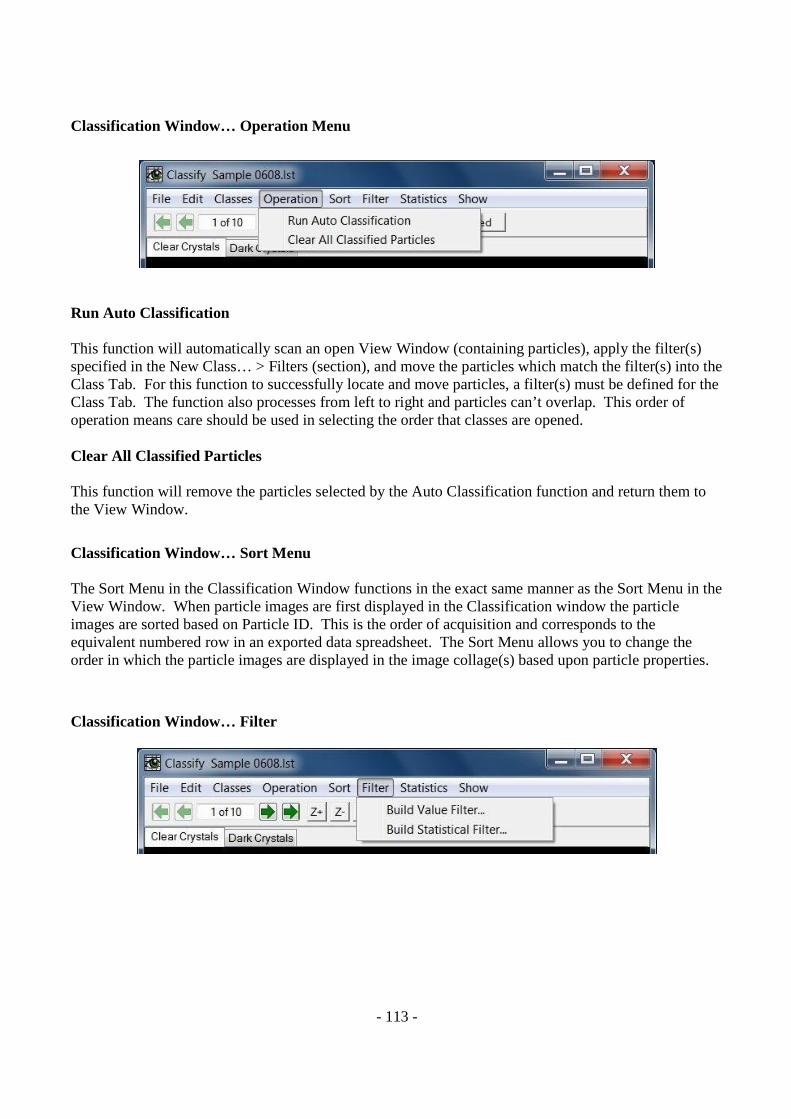
- 113 -

Classification Window… Operation Menu

Run Auto Classification This function will automatically scan an open View Window (containing particles), apply the filter(s) specified in the New Class… > Filters (section), and move the particles which match the filter(s) into the Class Tab. For this function to successfully locate and move particles, a filter(s) must be defined for the Class Tab. The function also processes from left to right and particles can’t overlap. This order of operation means care should be used in selecting the order that classes are opened. Clear All Classified Particles This function will remove the particles selected by the Auto Classification function and return them to the View Window.

Classification Window… Sort Menu The Sort Menu in the Classification Window functions in the exact same manner as the Sort Menu in the View Window. When particle images are first displayed in the Classification window the particle images are sorted based on Particle ID. This is the order of acquisition and corresponds to the equivalent numbered row in an exported data spreadsheet. The Sort Menu allows you to change the order in which the particle images are displayed in the image collage(s) based upon particle properties.

Classification Window… Filter

- 114 -

Build Value Filter… Selecting this function will open a Filter dialog box and automatically populate the Currently Using section with all available fields and their corresponding values. These values are derived from the Class Tab that is highlighted. This menu item allows the user to build a filter using the particle properties/characteristics of a Class. This is a value filter (a filter based on parameter measurements). Build Statistical Filter… Selecting this function will open a Filter dialog box and automatically populate the Currently Using section with all available fields and their corresponding values. These values are derived from the Class Tab that is highlighted. This menu item allows the user to build a filter using the particle properties/characteristics of a Class. This is a statistical filter (a filter based on derived statistics).

Classification Window… Statistics Menu Summary Statistics… This window provides statistics on the particle properties for particle images being viewed in the currently selected Class tab.

Classification Window… Show Menu Particle Properties (F8) Shows or hides the Particle Properties window. Moving the cursor over any particle image causes particle properties to be displayed in the Particle Properties window. Images (F9) Shows or hides the display of particle images. This menu command does not affect the number of particle images included in the Summary Statistics calculations or the exporting of particle property data. Ruler Shows or hides the Ruler line at the bottom of the Classification Window Image Collage.

Right Click Popup Menu To use the Popup Menu in the Classification Window, right click on one of the particle images. Remove Particle: Removes the particle image from the currently selected Class tab. Add To Library: Adds the particle to any Library Tab currently open in the Library Window. The Library window must be open with at least one Library open in it.

- 115 -

Move to Class: Moves the particle to another Class within the currently open Data set. More than one Class must be open in the Classify window.

Keyboard Commands Selecting Multiple Particle Images: To select a group of particle images within the Classification Window, press and hold the Ctrl key, click to the left of the first particle of interest, hold down on the mouse button and drag across the remaining particle(s) of interest.

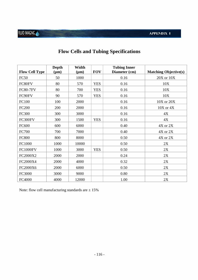
- 116 -

Flow Cells and Tubing Specifications

Flow Cell Type Depth (µm)

Width (µm) FOV

Tubing Inner Diameter (cm) Matching Objective(s)

FC50 50 1000 0.16 20X or 10X

FC80FV 80 570 YES 0.16 10X

FC80-7FV 80 700 YES 0.16 10X

FC90FV 90 570 YES 0.16 10X

FC100 100 2000 0.16 10X or 20X

FC200 200 2000 0.16 10X or 4X

FC300 300 3000 0.16 4X

FC300FV 300 1500 YES 0.16 4X

FC600 600 6000 0.40 4X or 2X

FC700 700 7000 0.40 4X or 2X

FC800 800 8000 0.50 4X or 2X

FC1000 1000 10000 0.50 2X

FC1000FV 1000 3000 YES 0.50 2X

FC2000X2 2000 2000 0.24 2X

FC2000X4 2000 4000 0.32 2X

FC2000X6 2000 6000 0.50 2X

FC3000 3000 9000 0.80 2X

FC4000 4000 12000 1.00 2X Note: flow cell manufacturing standards are ± 15%

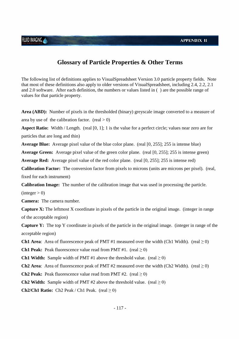
- 117 -

Glossary of Particle Properties & Other Terms

The following list of definitions applies to VisualSpreadsheet Version 3.0 particle property fields. Note that most of these definitions also apply to older versions of VisualSpreadsheet, including 2.4, 2.2, 2.1 and 2.0 software. After each definition, the numbers or values listed in ( ) are the possible range of values for that particle property. Area (ABD): Number of pixels in the thresholded (binary) greyscale image converted to a measure of

area by use of the calibration factor. (real > 0)

Aspect Ratio: Width / Length. (real [0, 1]; 1 is the value for a perfect circle; values near zero are for

particles that are long and thin)

Average Blue: Average pixel value of the blue color plane. (real [0, 255]; 255 is intense blue)

Average Green: Average pixel value of the green color plane. (real [0, 255]; 255 is intense green)

Average Red: Average pixel value of the red color plane. (real [0, 255]; 255 is intense red)

Calibration Factor: The conversion factor from pixels to microns (units are microns per pixel). (real,

fixed for each instrument)

Calibration Image: The number of the calibration image that was used in processing the particle.

(integer > 0)

Camera: The camera number.

Capture X: The leftmost X coordinate in pixels of the particle in the original image. (integer in range

of the acceptable region)

Capture Y: The top Y coordinate in pixels of the particle in the original image. (integer in range of the

acceptable region)

Ch1 Area: Area of fluorescence peak of PMT #1 measured over the width (Ch1 Width). (real ≥ 0)

Ch1 Peak: Peak fluorescence value read from PMT #1. (real ≥ 0)

Ch1 Width: Sample width of PMT #1 above the threshold value. (real ≥ 0)

Ch2 Area: Area of fluorescence peak of PMT #2 measured over the width (Ch2 Width). (real ≥ 0)

Ch2 Peak: Peak fluorescence value read from PMT #2. (real ≥ 0)

Ch2 Width: Sample width of PMT #2 above the threshold value. (real ≥ 0)

Ch2/Ch1 Ratio: Ch2 Peak / Ch1 Peak. (real ≥ 0)

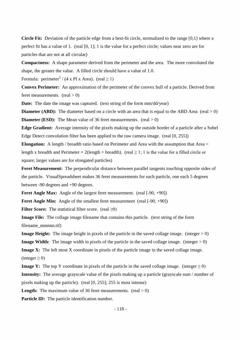
- 118 -

Circle Fit: Deviation of the particle edge from a best-fit circle, normalized to the range [0,1] where a

perfect fit has a value of 1. (real [0, 1]; 1 is the value for a perfect circle; values near zero are for

particles that are not at all circular)

Compactness: A shape parameter derived from the perimeter and the area. The more convoluted the

shape, the greater the value. A filled circle should have a value of 1.0.

Formula: perimeter2 / (4 x PI x Area). (real ≥ 1)

Convex Perimeter: An approximation of the perimeter of the convex hull of a particle. Derived from

feret measurements. (real > 0)

Date: The date the image was captured. (text string of the form mm/dd/year)

Diameter (ABD): The diameter based on a circle with an area that is equal to the ABD Area (real > 0)

Diameter (ESD): The Mean value of 36 feret measurements. (real > 0)

Edge Gradient: Average intensity of the pixels making up the outside border of a particle after a Sobel

Edge Detect convolution filter has been applied to the raw camera image. (real [0, 255])

Elongation: A length / breadth ratio based on Perimeter and Area with the assumption that Area =

length x breadth and Perimeter = 2(length + breadth). (real ≥ 1; 1 is the value for a filled circle or

square; larger values are for elongated particles)

Feret Measurement: The perpendicular distance between parallel tangents touching opposite sides of

the particle. VisualSpreadsheet makes 36 feret measurements for each particle, one each 5 degrees

between -90 degrees and +90 degrees.

Feret Angle Max: Angle of the largest feret measurement. (real [-90, +90])

Feret Angle Min: Angle of the smallest feret measurement (real [-90, +90])

Filter Score: The statistical filter score. (real ≥0)

Image File: The collage image filename that contains this particle. (text string of the form

filename_nnnnnn.tif)

Image Height: The image height in pixels of the particle in the saved collage image. (integer > 0)

Image Width: The image width in pixels of the particle in the saved collage image. (integer > 0)

Image X: The left most X coordinate in pixels of the particle image in the saved collage image.

(integer ≥ 0)

Image Y: The top Y coordinate in pixels of the particle in the saved collage image. (integer ≥ 0)

Intensity: The average grayscale value of the pixels making up a particle (grayscale sum / number of

pixels making up the particle). (real [0, 255]; 255 is most intense)

Length: The maximum value of 36 feret measurements. (real > 0)

Particle ID: The particle identification number.

- 119 -

PPC (Particles Per Chain): The number of particles that were grouped into one particle based on the

nearest neighbor distance. (integer > 0; always 1 if nearest neighbor distance is 0)

Perimeter: Total length of the edges making up a particle including the edges of any holes. (real > 0)

Ratio Blue/Green: Average Blue / Average Green. (real ≥ 0)

Ratio Red/Blue: Average Red / Average Blue. (real ≥ 0)

Ratio Red/Green: Average Red / Average Green. (real ≥ 0)

Roughness: A measure of the unevenness or irregularity of a particle's surface-the ratio of perimeter to

convex perimeter. (real ≥ 1; 1 is the value for a filled shape with convex perimeter; larger values are for

particles that have interior holes and/or a non-convex perimeter)

Scatter Area: Area of the peak of the scatter detector measured over the width. (real ≥ 0)

Scatter Peak: Peak value read from the scatter detector. (real ≥ 0)

Scatter Width: Sample width of scatter detector values above the scatter threshold. (real ≥ 0)

Sigma Intensity: Standard deviation of grayscale values. (real ≥ 0)

Source Image: The camera image number or raw file image number where the particle was captured.

(integer > 0)

Sum Intensity: Sum of grayscale pixel values. (real > 0)

Time: The time that the image was captured.

Timestamp: The time the image was captured in milliseconds.

Transparency: 1 – (ABD Diameter / ESD Diameter). (real [0, 1]; 0 is the value for a filled circle;

values near 1 are for an elongated or irregular shape or a shape that has many interior holes)

Volume (ABD): Sphere volume calculated from ABD Diameter. (real > 0)

Volume (ESD): Sphere volume calculated from ESD Diameter. (real > 0)

Width: The minimum value of 36 feret measurements. (real > 0)

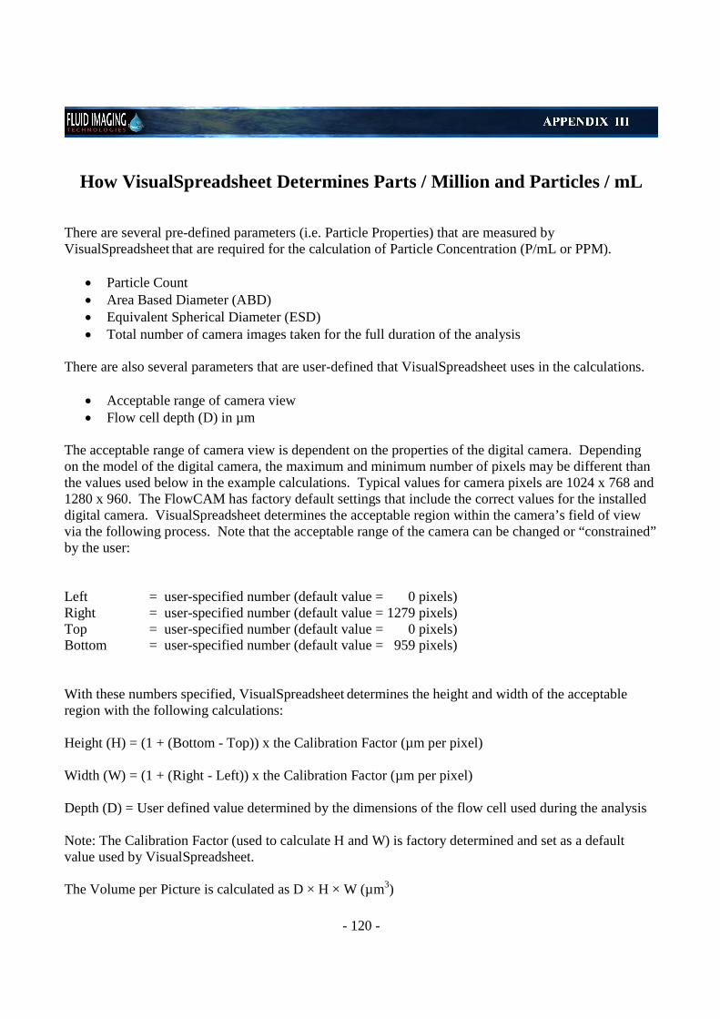
- 120 -

How VisualSpreadsheet Determines Parts / Million and Particles / mL There are several pre-defined parameters (i.e. Particle Properties) that are measured by VisualSpreadsheet that are required for the calculation of Particle Concentration (P/mL or PPM).

· Particle Count · Area Based Diameter (ABD) · Equivalent Spherical Diameter (ESD) · Total number of camera images taken for the full duration of the analysis

There are also several parameters that are user-defined that VisualSpreadsheet uses in the calculations.

· Acceptable range of camera view · Flow cell depth (D) in µm

The acceptable range of camera view is dependent on the properties of the digital camera. Depending on the model of the digital camera, the maximum and minimum number of pixels may be different than the values used below in the example calculations. Typical values for camera pixels are 1024 x 768 and 1280 x 960. The FlowCAM has factory default settings that include the correct values for the installed digital camera. VisualSpreadsheet determines the acceptable region within the camera’s field of view via the following process. Note that the acceptable range of the camera can be changed or “constrained” by the user: Left = user-specified number (default value = 0 pixels) Right = user-specified number (default value = 1279 pixels) Top = user-specified number (default value = 0 pixels) Bottom = user-specified number (default value = 959 pixels) With these numbers specified, VisualSpreadsheet determines the height and width of the acceptable region with the following calculations: Height (H) = (1 + (Bottom - Top)) x the Calibration Factor (µm per pixel)

Width (W) = (1 + (Right - Left)) x the Calibration Factor (µm per pixel) Depth (D) = User defined value determined by the dimensions of the flow cell used during the analysis

Note: The Calibration Factor (used to calculate H and W) is factory determined and set as a default value used by VisualSpreadsheet.

The Volume per Picture is calculated as D × H × W (µm3)

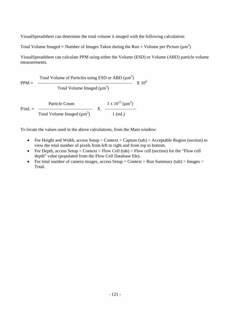
- 121 -

VisualSpreadsheet can determine the total volume it imaged with the following calculation: Total Volume Imaged = Number of Images Taken during the Run × Volume per Picture (µm3)

VisualSpreadsheet can calculate PPM using either the Volume (ESD) or Volume (ABD) particle volume measurements. Total Volume of Particles using ESD or ABD (µm3) PPM = ————————————————————— X 106 Total Volume Imaged (µm3) Particle Count 1 x 1012 (µm3) P/mL = ———————————— X ——————— Total Volume Imaged (µm3) 1 (mL) To locate the values used in the above calculations, from the Main window:

· For Height and Width, access Setup > Context > Capture (tab) > Acceptable Region (section) to view the total number of pixels from left to right and from top to bottom.

· For Depth, access Setup > Context > Flow Cell (tab) > Flow cell (section) for the “Flow cell depth” value (populated from the Flow Cell Database file).

· For total number of camera images, access Setup > Context > Run Summary (tab) > Images > Total.

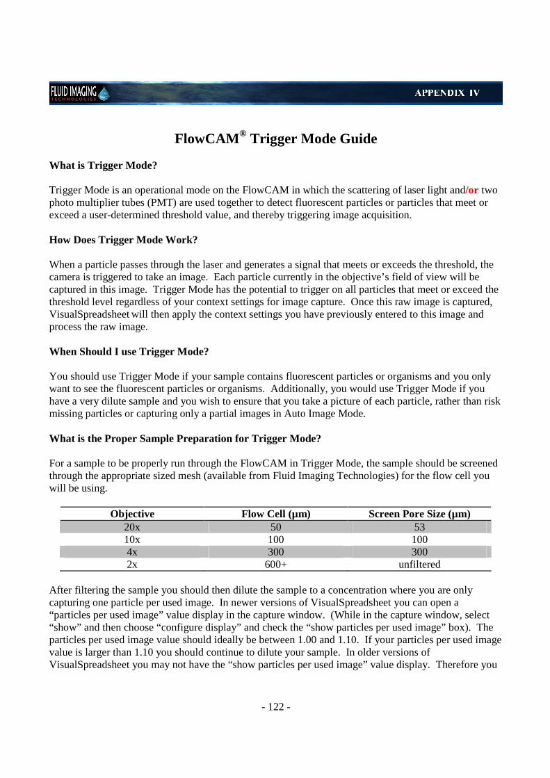
- 122 -

FlowCAM® Trigger Mode Guide

What is Trigger Mode? Trigger Mode is an operational mode on the FlowCAM in which the scattering of laser light and/or two photo multiplier tubes (PMT) are used together to detect fluorescent particles or particles that meet or exceed a user-determined threshold value, and thereby triggering image acquisition. How Does Trigger Mode Work? When a particle passes through the laser and generates a signal that meets or exceeds the threshold, the camera is triggered to take an image. Each particle currently in the objective’s field of view will be captured in this image. Trigger Mode has the potential to trigger on all particles that meet or exceed the threshold level regardless of your context settings for image capture. Once this raw image is captured, VisualSpreadsheet will then apply the context settings you have previously entered to this image and process the raw image. When Should I use Trigger Mode? You should use Trigger Mode if your sample contains fluorescent particles or organisms and you only want to see the fluorescent particles or organisms. Additionally, you would use Trigger Mode if you have a very dilute sample and you wish to ensure that you take a picture of each particle, rather than risk missing particles or capturing only a partial images in Auto Image Mode. What is the Proper Sample Preparation for Trigger Mode? For a sample to be properly run through the FlowCAM in Trigger Mode, the sample should be screened through the appropriate sized mesh (available from Fluid Imaging Technologies) for the flow cell you will be using.

Objective Flow Cell (µm) Screen Pore Size (µm)

20x 50 53 10x 100 100 4x 300 300 2x 600+ unfiltered

After filtering the sample you should then dilute the sample to a concentration where you are only capturing one particle per used image. In newer versions of VisualSpreadsheet you can open a “particles per used image” value display in the capture window. (While in the capture window, select “show” and then choose “configure display” and check the “show particles per used image” box). The particles per used image value should ideally be between 1.00 and 1.10. If your particles per used image value is larger than 1.10 you should continue to dilute your sample. In older versions of VisualSpreadsheet you may not have the “show particles per used image” value display. Therefore you

- 123 -

will have to use a trial and error approach until you are obtaining as close to one particle per used image as possible. How to Run a Trigger Mode Sample

1. Turn on the laser and allow it to warm up. Usually about fifteen minutes is sufficient for this

purpose. 2. Determine and set your initial “Context” settings. 3. Introduce your sample to the FlowCAM. 4. Click on the “Setup” menu option at the top of VisualSpreadsheet Main window and select “Set

Up and Focus” and focus your FlowCAM. 5. Click on the “Setup” menu option at the top of the VisualSpreadsheet Main window and select

“Trigger Mode Setup”. 6. If possible, open the “Particles per Used Image” value display. 7. Determine if sample is too concentrated and dilute as needed. 8. Change “Context” settings if necessary. 9. Close “Trigger Mode Set Up”. 10. Click on the “Setup” menu option at the top of the VisualSpreadsheet Main window and select

“Trigger Mode (No Save)”. 11. Determine if your focus is correct and if sample is too concentrated, dilute as necessary. 12. Close “Trigger Mode (No Save)” once concentration and focus are both deemed to be

appropriate. 13. Click on the “Analysis” menu option at the top of the VisualSpreadsheet Main window. 14. Select “Trigger Mode”. 15. Input your desired stop criteria and click “OK”. 16. Save the run in an appropriate location with any file name you wish and click “Save”. 17. Allow run to finish. Repeat above steps for each sample.

Factors that May Affect the Results of Your Trigger Mode Run

Once you have successfully completed a run, it is important to note that there are a few factors that may affect the performance of your FlowCAM in Trigger Mode. When using a FlowCAM, your objective lens does not view the entire width of the flow cell. If you are using the FlowCAM for counting purposes, you may want to consider using a Field of View (FOV) flow cell - this will allow you to image the entire fluid stream (for more information please contact the Fluid Imaging Technologies, Inc. Sales Department). If you are not suspending your sample in a dense/viscous fluid, or you are not occasionally stirring the sample in the funnel, you may get a settling effect. You may notice that as the fluid level in your funnel decreases particles may stick to the side of the funnel. If you see this settling affect you may want to carefully mix the funnel contents. During a run you can also open the Time Series Graph. Select “Tools” and then click “Time Series Graph”. When the “Frequency Plot” is selected, you may notice a gradual decrease in the slope of the trend line. This decrease may mean that your sample is slowly

- 124 -

settling. Note that you can view this graph in “real time” as you are running your sample. It is possible to capture images of particles that did not trigger the laser or the PMT. This happens because once the threshold level is met or exceeded, the camera takes a raw image, and collages the raw image based on your context settings. If there is more than one particle in the raw image, VisualSpreadsheet has no way to determine which particle produced the trigger event. Therefore the same particle properties (related to the trigger event, such as CH1 Peak) are assigned to all particles within that raw image. This is the main reason that your sample should be as close to “One Particle per Used Image” as possible. The rate at which you set your pump can also influence both the image quality and number of particles you will collect. If the pump speed is too fast, you may find that the particle that caused the triggering event is already out of the objective’s field of view before the camera can take an image. This means that you may have zero particles being captured in your raw images. Slowing down the pump speed can help alleviate this problem.

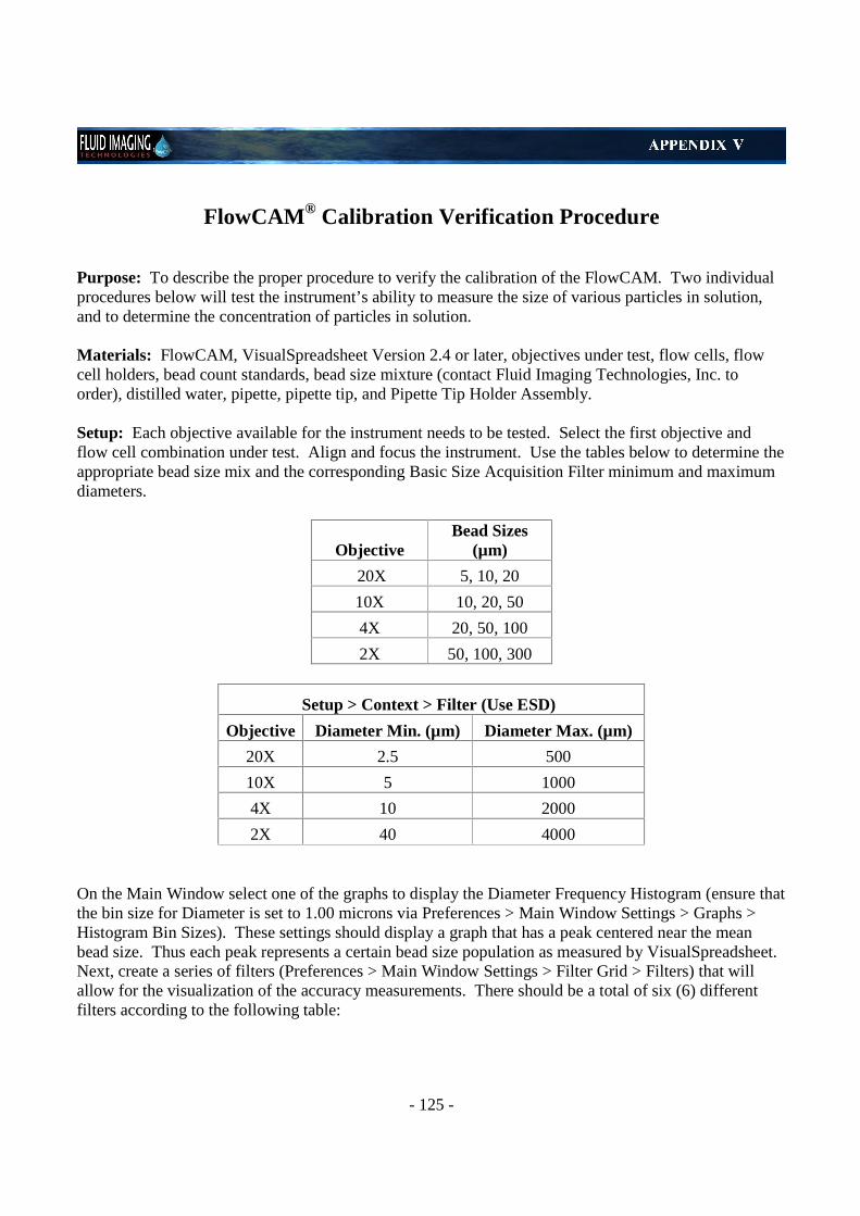
- 125 -

FlowCAM® Calibration Verification Procedure Purpose: To describe the proper procedure to verify the calibration of the FlowCAM. Two individual procedures below will test the instrument’s ability to measure the size of various particles in solution, and to determine the concentration of particles in solution. Materials: FlowCAM, VisualSpreadsheet Version 2.4 or later, objectives under test, flow cells, flow cell holders, bead count standards, bead size mixture (contact Fluid Imaging Technologies, Inc. to order), distilled water, pipette, pipette tip, and Pipette Tip Holder Assembly. Setup: Each objective available for the instrument needs to be tested. Select the first objective and flow cell combination under test. Align and focus the instrument. Use the tables below to determine the appropriate bead size mix and the corresponding Basic Size Acquisition Filter minimum and maximum diameters.

Objective Bead Sizes

(µm)

20X 5, 10, 20

10X 10, 20, 50

4X 20, 50, 100

2X 50, 100, 300

Setup > Context > Filter (Use ESD)

Objective Diameter Min. (µm) Diameter Max. (µm)

20X 2.5 500

10X 5 1000

4X 10 2000

2X 40 4000 On the Main Window select one of the graphs to display the Diameter Frequency Histogram (ensure that the bin size for Diameter is set to 1.00 microns via Preferences > Main Window Settings > Graphs > Histogram Bin Sizes). These settings should display a graph that has a peak centered near the mean bead size. Thus each peak represents a certain bead size population as measured by VisualSpreadsheet. Next, create a series of filters (Preferences > Main Window Settings > Filter Grid > Filters) that will allow for the visualization of the accuracy measurements. There should be a total of six (6) different filters according to the following table:

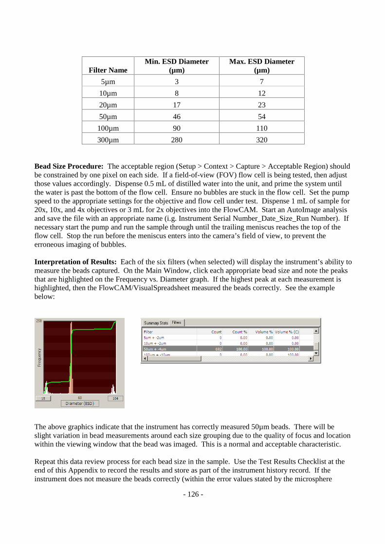
- 126 -

Filter Name Min. ESD Diameter

(µm) Max. ESD Diameter

(µm)

5µm 3 7

10µm 8 12

20µm 17 23

50µm 46 54

100µm 90 110

300µm 280 320 Bead Size Procedure: The acceptable region (Setup > Context > Capture > Acceptable Region) should be constrained by one pixel on each side. If a field-of-view (FOV) flow cell is being tested, then adjust those values accordingly. Dispense 0.5 mL of distilled water into the unit, and prime the system until the water is past the bottom of the flow cell. Ensure no bubbles are stuck in the flow cell. Set the pump speed to the appropriate settings for the objective and flow cell under test. Dispense 1 mL of sample for 20x, 10x, and 4x objectives or 3 mL for 2x objectives into the FlowCAM. Start an AutoImage analysis and save the file with an appropriate name (i.g. Instrument Serial Number_Date_Size_Run Number). If necessary start the pump and run the sample through until the trailing meniscus reaches the top of the flow cell. Stop the run before the meniscus enters into the camera’s field of view, to prevent the erroneous imaging of bubbles. Interpretation of Results: Each of the six filters (when selected) will display the instrument’s ability to measure the beads captured. On the Main Window, click each appropriate bead size and note the peaks that are highlighted on the Frequency vs. Diameter graph. If the highest peak at each measurement is highlighted, then the FlowCAM/VisualSpreadsheet measured the beads correctly. See the example below:

The above graphics indicate that the instrument has correctly measured 50µm beads. There will be slight variation in bead measurements around each size grouping due to the quality of focus and location within the viewing window that the bead was imaged. This is a normal and acceptable characteristic. Repeat this data review process for each bead size in the sample. Use the Test Results Checklist at the end of this Appendix to record the results and store as part of the instrument history record. If the instrument does not measure the beads correctly (within the error values stated by the microsphere

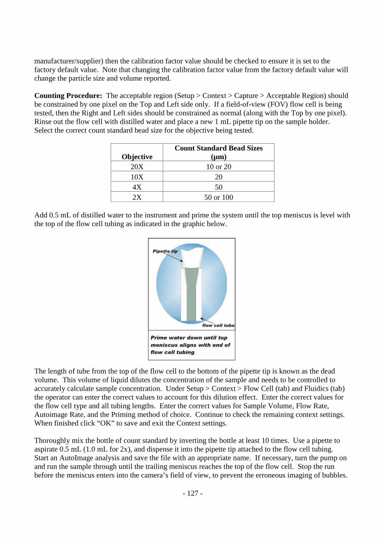
- 127 -

Prime water down until top meniscus aligns with end of flow cell tubing.

flow cell tube

Pipette tip

manufacturer/supplier) then the calibration factor value should be checked to ensure it is set to the factory default value. Note that changing the calibration factor value from the factory default value will change the particle size and volume reported. Counting Procedure: The acceptable region (Setup > Context > Capture > Acceptable Region) should be constrained by one pixel on the Top and Left side only. If a field-of-view (FOV) flow cell is being tested, then the Right and Left sides should be constrained as normal (along with the Top by one pixel). Rinse out the flow cell with distilled water and place a new 1 mL pipette tip on the sample holder. Select the correct count standard bead size for the objective being tested.

Objective Count Standard Bead Sizes

(µm) 20X 10 or 20 10X 20 4X 50 2X 50 or 100

Add 0.5 mL of distilled water to the instrument and prime the system until the top meniscus is level with the top of the flow cell tubing as indicated in the graphic below. The length of tube from the top of the flow cell to the bottom of the pipette tip is known as the dead volume. This volume of liquid dilutes the concentration of the sample and needs to be controlled to accurately calculate sample concentration. Under Setup > Context > Flow Cell (tab) and Fluidics (tab) the operator can enter the correct values to account for this dilution effect. Enter the correct values for the flow cell type and all tubing lengths. Enter the correct values for Sample Volume, Flow Rate, Autoimage Rate, and the Priming method of choice. Continue to check the remaining context settings. When finished click “OK” to save and exit the Context settings. Thoroughly mix the bottle of count standard by inverting the bottle at least 10 times. Use a pipette to aspirate 0.5 mL (1.0 mL for 2x), and dispense it into the pipette tip attached to the flow cell tubing. Start an AutoImage analysis and save the file with an appropriate name. If necessary, turn the pump on and run the sample through until the trailing meniscus reaches the top of the flow cell. Stop the run before the meniscus enters into the camera’s field of view, to prevent the erroneous imaging of bubbles.

- 128 -

Post process the resulting data (saving the new data set as a separate list file) to remove any non-bead or particles that might have been imaged during the run (either by using a pre-defined filter, or manually selecting particles from the View Window). Open the newly saved post-processed list file. The Particles/mL value will be displayed on the Main Window and via the ‘Statistics’ menu item in the View Window. Interpretation of Results: The Particles/mL value will be displayed on the Main Window and via the ‘Statistics’ menu item in the View Window. Use the Test Results Checklist at the end of this Appendix to record the results and store as part of the instrument history record. If the instrument does not measure the concentration correctly (within the error values stated by the count standard manufacturer/supplier) then the above counting procedure should be repeated to double check the out of tolerance results.

- 129 -

Serial No.: Test Date:

Model No.:

Size Procedure

Bead Mix Pass/Fail

2X Bead Mix

4X Bead Mix

10X Bead Mix

20X Bead Mix

Count Procedure

Objective Bead Size

(µm) Listed Count

(P/mL) FlowCAM Count (P/mL) Pass/Fail

2X

4X

10X

20X

If a particular objective was not required/available for testing enter “N/A”

Notes (reagent lot numbers, etc.):

Testing Performed By:

__________________________________________ _________________________________

Signature / Printed Name Title

- 130 -

FlowCAM® Quick Start Guide

Before You Start

· Flow cells should be clean of contaminants (both inside and out) as best as possible. · Keep the workbench and area free of vibrations or movement while performing an analysis. · Refer to the FlowCAM Manual, and other supplemental training documents, for more

information and tips. · If using a new flow cell the tubing ends will need to be cut. A length of 8-10 cm for the top

tubing and 20-30 cm for the bottom tubing is the standard recommendation. If a flow cell is being reused, measure the tubing above and below the flow cell while it is lying flat before installing it into the FlowCAM.

Step-By-Step Instructions

1. Insure that the license dongle is plugged into a USB port on the FlowCAM (not applicable to all

FlowCAM models).

2. Turn on the FlowCAM using the power switches located on the rear and front of the instrument.

3. Wait for the operating system to fully load.

4. Set up the hardware in the following order:

§ Attach sample introduction stand

§ Screw in collimator/diffuser if required

§ Screw in objective

§ Clean the flow cell

§ Place flow cell in the correct flow cell holder (QCFC)

§ Place flow cell and flow cell holder onto the flow cell holder mount

§ Lower sample introduction tray down over the tubing from the flow cell

§ Gently push pipette tip down into the flow cell tubing until tubing starts to expand

§ Lift sample introduction tray up until the flow cell tubing is taut but not over stretched

§ Insure that tubing from the flow cell to the pipette tip is as straight as possible

§ Prepare pump (refer to the correct section in the FlowCAM Manual for more information)

§ Attach flow cell tubing to pump

- 131 -

§ Attach waste tubing to pump

§ Insure that waste tubing is going to a waste container

§ Center the fine focus travel if required

5. Setup the software/hardware in the following order:

§ Open Visual Spreadsheet and select the correct objective

§ Insure that the Status Bar color (if displayed) at the bottom of the Main Window matches the

colored stripe on the installed objective

§ Main Window: Setup > Setup and Focus

· Focus on the flow cell using the coarse adjustment Z translator

· Use the Course Adjustment screw on the Z translator to lock the Z translator into place

· Add the sample and turn on the pump until the sample can be seen in the Setup and Focus

window. Note: Proper sample preparation is critical to having a successful FlowCAM

analysis. It is important to get the proper particle size distribution and sample dilution to

ensure that the best possible data are obtained.

· Use the fine focus adjustment knob to adjust the focus until the sample appears to look

the best possible

· Setup and Focus window: Setup > Camera

· Move the Camera Settings window so that it is not overlaying the Setup and Focus

window (Note: You must click “Apply” for any changes in the Camera window to take

effect).

¨ Adjust the U and V color balance until the displayed camera image is a uniform gray

background (only necessary for a color camera)

¨ Adjust the Gain and Flash Duration (increased gain and flash duration will result in a

higher intensity mean) until you have an intensity mean of 165-185

¨ Close the Camera window

· Determine the concentration, coloration, and size distribution of the sample by looking at

the particles that are displayed in the setup and focus window

§ Close the Setup and Focus window

§ Main Window: Setup > Context

· Context Window: Adjust the context settings via the following tabs:

¨ Capture

¨ Flow Cell

- 132 -

¨ Fluidics

¨ Filter

¨ PMT/Scatter (if required)

¨ Stop

¨ Load (if desired)

· Click OK in the Context Window

§ Test the settings before you do an analysis by starting AutoImage Mode (No Save) or Trigger

Mode (No Save).

§ Main Window: Setup > AutoImage Mode (No Save) or Trigger Mode (No Save). Note: If

working with a peristaltic style pump, turn on the pump before you click on the No Save

mode.

· Determine if the FlowCAM is identifying particles of interest to you and segmenting

them correctly.

· Close the No Save run and make changes in the Context Settings and repeat as needed

§ Insure that an appropriate amount of sample is in the sample introduction funnel/pipette

§ Main Window: Analyze > Mode of your choice

· Follow subsequent prompts

· In the window where the data set is named please note that when you click “Save” the

run will begin

§ Allow data collection to end based on the preset stop conditions or terminate manually if

desired/required.

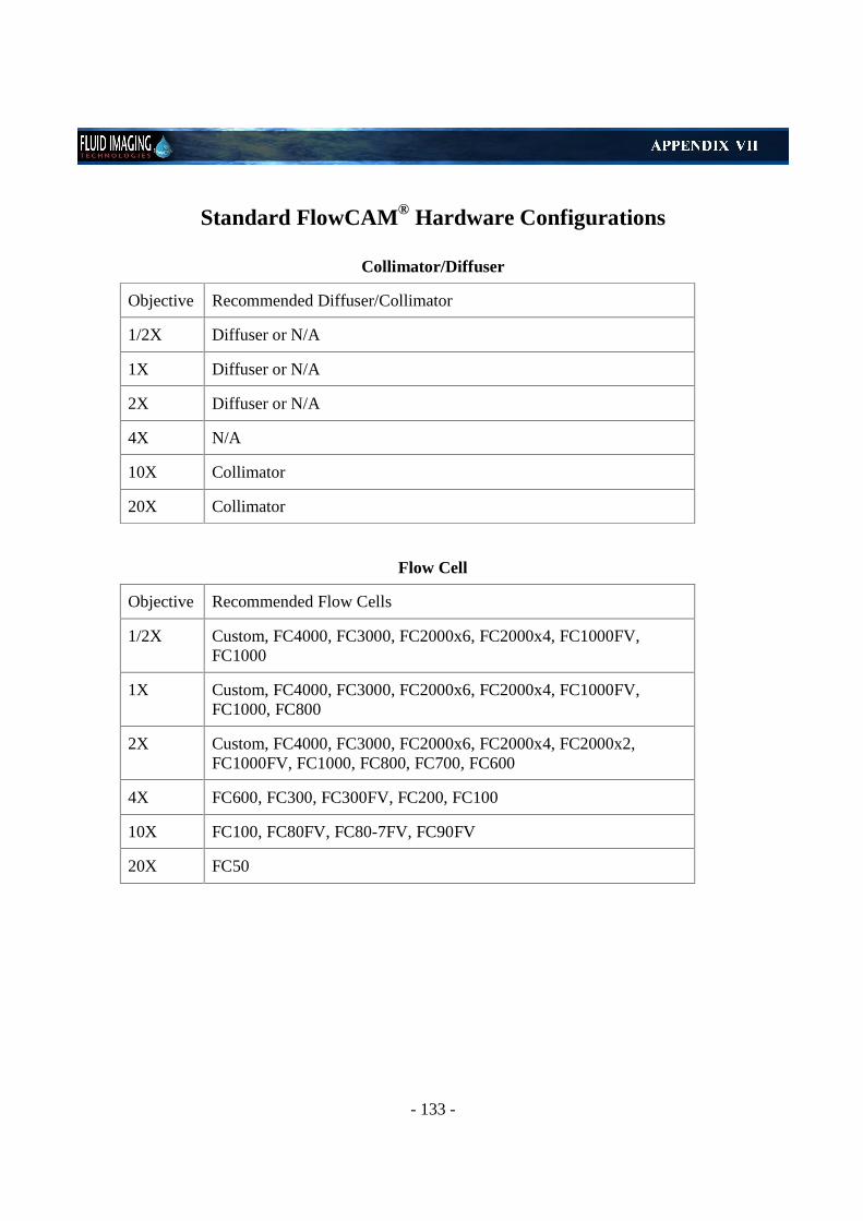
- 133 -

Standard FlowCAM® Hardware Configurations

Collimator/Diffuser

Objective Recommended Diffuser/Collimator

1/2X Diffuser or N/A

1X Diffuser or N/A

2X Diffuser or N/A

4X N/A

10X Collimator

20X Collimator

Flow Cell

Objective Recommended Flow Cells

1/2X Custom, FC4000, FC3000, FC2000x6, FC2000x4, FC1000FV, FC1000

1X Custom, FC4000, FC3000, FC2000x6, FC2000x4, FC1000FV, FC1000, FC800

2X Custom, FC4000, FC3000, FC2000x6, FC2000x4, FC2000x2, FC1000FV, FC1000, FC800, FC700, FC600

4X FC600, FC300, FC300FV, FC200, FC100

10X FC100, FC80FV, FC80-7FV, FC90FV

20X FC50

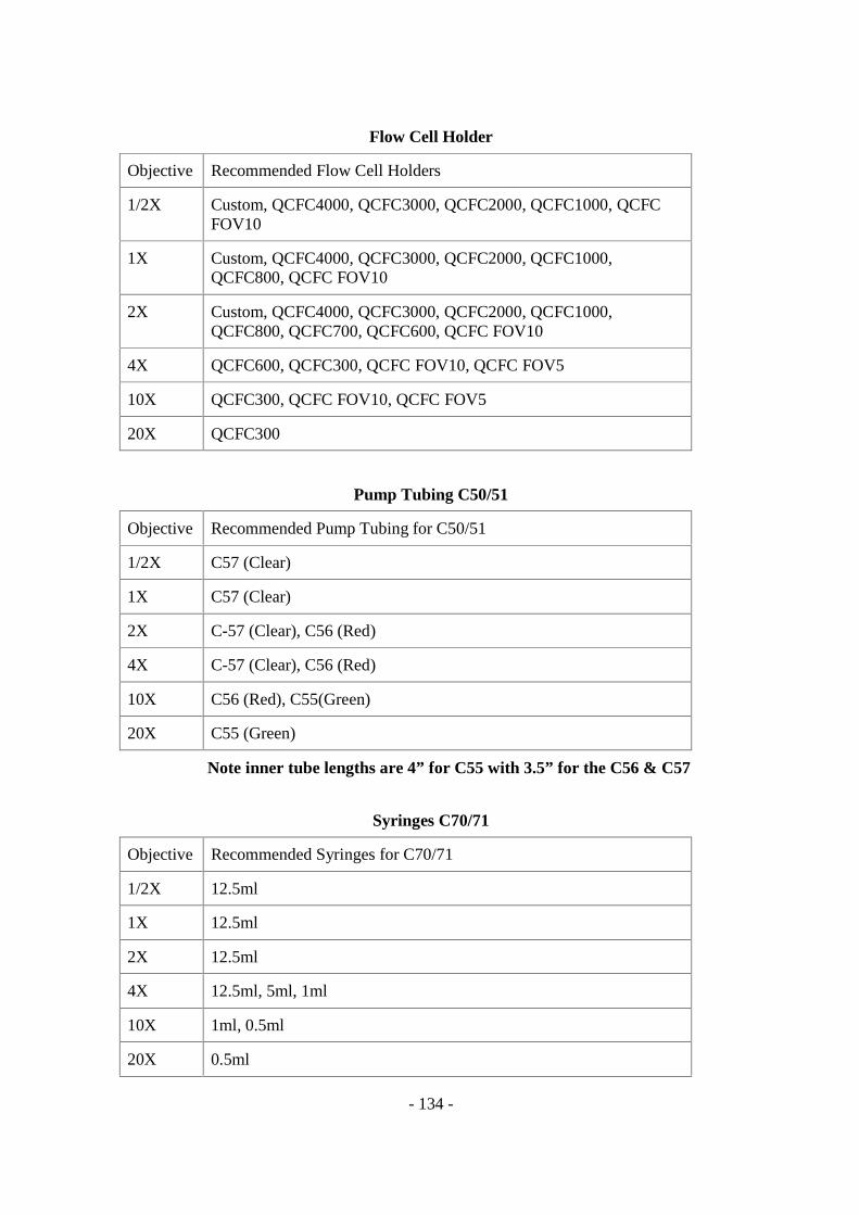
- 134 -

Flow Cell Holder

Objective Recommended Flow Cell Holders

1/2X Custom, QCFC4000, QCFC3000, QCFC2000, QCFC1000, QCFC FOV10

1X Custom, QCFC4000, QCFC3000, QCFC2000, QCFC1000, QCFC800, QCFC FOV10

2X Custom, QCFC4000, QCFC3000, QCFC2000, QCFC1000, QCFC800, QCFC700, QCFC600, QCFC FOV10

4X QCFC600, QCFC300, QCFC FOV10, QCFC FOV5

10X QCFC300, QCFC FOV10, QCFC FOV5

20X QCFC300

Pump Tubing C50/51

Objective Recommended Pump Tubing for C50/51

1/2X C57 (Clear)

1X C57 (Clear)

2X C-57 (Clear), C56 (Red)

4X C-57 (Clear), C56 (Red)

10X C56 (Red), C55(Green)

20X C55 (Green)

Note inner tube lengths are 4” for C55 with 3.5” for the C56 & C57

Syringes C70/71

Objective Recommended Syringes for C70/71

1/2X 12.5ml

1X 12.5ml

2X 12.5ml

4X 12.5ml, 5ml, 1ml

10X 1ml, 0.5ml

20X 0.5ml

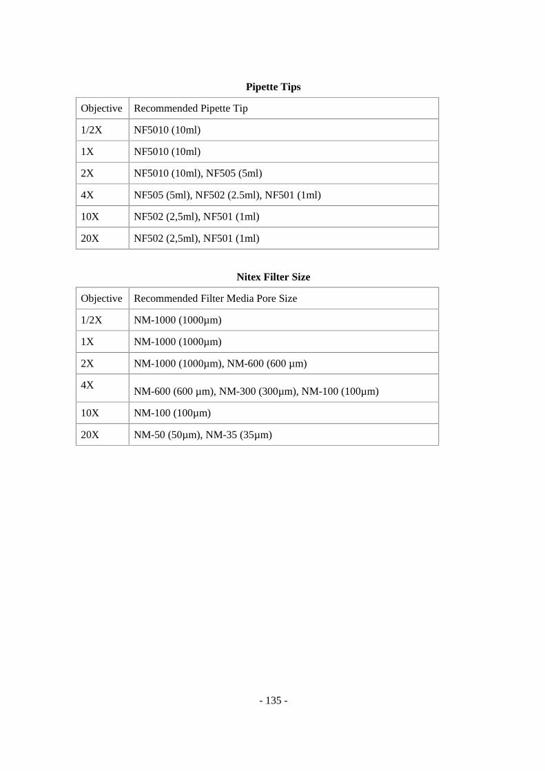
- 135 -

Pipette Tips

Objective Recommended Pipette Tip

1/2X NF5010 (10ml)

1X NF5010 (10ml)

2X NF5010 (10ml), NF505 (5ml)

4X NF505 (5ml), NF502 (2.5ml), NF501 (1ml)

10X NF502 (2,5ml), NF501 (1ml)

20X NF502 (2,5ml), NF501 (1ml)

Nitex Filter Size

Objective Recommended Filter Media Pore Size

1/2X NM-1000 (1000µm)

1X NM-1000 (1000µm)

2X NM-1000 (1000µm), NM-600 (600 µm)

4X NM-600 (600 µm), NM-300 (300µm), NM-100 (100µm)

10X NM-100 (100µm)

20X NM-50 (50µm), NM-35 (35µm)

- 136 -

Frequently Asked Questions (FAQ)

Q. Do I need to use a collimator or light diffuser with the particular objective I am using? A. Review the documentation that came with the instrument to determine the proper configurations. While the 2X Objective may require the use of a light diffuser, and the 10X and 20X Objectives usually require a light collimator, it ultimately depends on the specific configuration of your instrument. Q. How do I prevent particles that lie over the edge of the camera field of view from getting imaged? A. If your “acceptable region” is unconstrained (for example: Left = 0, Right = 1279, Top = 0, Bottom = 959), particles that lie across the edge of the field of view will be imaged as a partial particle. Once you constrain a side by at least one pixel (for example: Left = 1, Right = 1278, Top = 1, and Bottom = 958), any particle that lies across that boundary will NOT be considered a particle, and therefore, will not get imaged. Q. How can I test the effects of changing the value for the “close holes” function? A. The best way to demonstrate close small holes is to do a run of calibration beads, using dark pixels only and without close holes enabled (i.e., close holes iterations = 0). Be sure to save binary collage images and raw camera images for this run. Use the binarization overlay to demonstrate that the software did not use the pixels at the center of the image of a bead (because those pixels are lighter than the background calibration image). Now go into File Processing Mode and reprocess the raw images you collected, this time with close holes enabled (i.e., close holes iterations > 0). Repeat this process using more and more iterations of the close holes algorithm to show how the “hole” is filled (i.e. more and more of the pixels that are at the center of the bead are being used when calculating particle properties). Q. How is the size calibration determined? A. The calibration constants are determined during the manufacturing of the instrument and should never need to be changed. Fluid Imaging Technologies, Inc. uses a proprietary optical calibration device to determine the calibration factor of each objective for every instrument. The only time a unit should be recalibrated is if a major component along the optics path inside the instrument is replaced or damaged. In that specific instance, the FlowCAM should be returned to Fluid Imaging Technologies. The size calibration can be verified at any time using a mixture of calibrated microspheres (see Appendix V). The microsphere and test solutions can be purchased from Fluid Imaging Technologies or through your sales representative.

- 137 -

Q. How is the particle concentration determined? A. When running in AutoImage Mode, the camera is imaging the field of view at regular intervals. In this case, the number of camera images collected multiplied by the volume of each field of view image (length and width of the field of view times the depth of the flow cell), provides the total volume of the fluid that was "sampled" by the instrument. The particle concentration is the number of particles divided by the volume imaged; if the sample fluid was diluted or concentrated, and/or non-sample fluid was used to prime the system, the concentration is adjusted to be in terms of the original sample. When running in Trigger Mode where the camera takes an image only if a fluorescence and/or light scatter threshold is exceeded, two values provide the information necessary in order to calculate particle concentration: 1) the ratio of the field of view width to the flow cell width; 2) the number of milliliters analyzed. Note that VisualSpreadsheet makes the assumption that the particles are distributed uniformly across the flow cell in calculating the concentration in Trigger Mode. Q. How does the FlowCAM determine particle diameter? A. There are two ways that the software calculates diameter, Area Based Diameter (ABD) and Equivalent Spherical Diameter (ESD). ABD (Area Based Diameter) is the diameter of the circle with an area that is equal to the ABD Area of the particle. This diameter can also be thought of as the diameter of the circle obtained by arranging the pixels that comprise the thresholded particle in a solid circle. ESD (Equivalent Spherical Diameter) is the mean feret measurement of the particle based on 36 sample measurements (conducted every 5°). Q. Should I pre-filter my sample? A. If the sample contains a significant number of particles that have a diameter greater than the width of the flow cell, then the sample will need to be filtered to prevent clogging of the flow cell. Q. What are the different lasers and PMT/Filter sets that are available for use with the FlowCAM? A. The laser and PMT/Filter set is specified at the time of purchase for each FlowCAM. However, depending on the model of the FlowCAM, it may be possible to upgrade or use other lasers and/or filter sets. At this time, Fluid Imaging Technologies, Inc. builds FlowCAMs equipped with 532 nm or 488 nm lasers. The PMT/Filter sets available include Red/Orange [>650/575±15] and Red/Green [>650/525±15]. Q. When viewing the flow cell, I can see small particles that appear to be on the glass and some that don’t move when the flow cell is adjusted. How do I remove these particles? A. These small particles are typically dust and contamination that can be found on the inside and outside of the flow cells and on the outside of the objective lens. You can use high grade acetone or lens cleaning solution to clean the objectives and flow cells. Only use specially designed lens paper to avoid scratching any of the glass surfaces. Immediately after use, rinse the funnel and flow cell with deionized or distilled water. If necessary, precede this rinse with an appropriate solvent or surfactant in order to remove the particles. The rinse will help keep the flow cells clear and free from contamination for day-to-day use.

- 138 -

Q. My monitor has a blank/black screen and doesn’t appear to be working even though the power is on, what should I do? A. You can try to re-engage the monitor by holding down the Ctrl+Alt+F1 keys. Q. I’m not sure when I should use a Classification and when I should use a Library. Can you provide an example of the use of the Classification and Library Windows? A. A good way to describe the use of both Classification and Library files is to outline a typical (and intended) use of these features. An example is an oceanographic cruise where the ship is scheduled to visit 10 research stations. At station I, you collect a water sample and analyze it with the FlowCAM. During the transit from station I to station II, you classify all of the particles imaged into species A, B, C, etc. You do the same for stations II and III. Then, you pool all of the images collected for species A at stations 1, 2, and 3 into a single library. You pool all of the other classified species into individual libraries the same way. At this point, you have a library for each of the species, comprised of images that were captured at multiple stations (providing a larger data base of images). After collecting another sample and analyzing it at station IV, you can now sort your data by using the characteristics of each library (using them as filters). Note that when using a library for filtering, it is recommended that you only have 10-15 organisms in it to avoid introduction of error. Then, after refining these library-selected classifications, you would add these images (for species A, B, C, etc.) to their respective libraries. As you repeat this procedure at each station, the libraries you are using as filters grow in size and become better at recognizing (classifying) species. Q. How do I create a Statistical Filter from a Library of Images? A. Follow the procedure below to create a Library (if necessary) and then a Statistical Filter. To create a Library: 1. Main window: File > Open List 2. Main window: Edit > Show All Data [or F3] 3. Main window: Edit > Open View Window [or F2] 4. View window: select (highlight) 3-5 like particles of interest 5. View window: Filter > Like Selected Particles (Statistical) [or F5] 6. View window: select (highlight) all like particles of interest 7. View window: Edit > Delete Images NOT selected 8. View window: File > Save as Library > name, then click the Save button 9. Close the View window To use a Library to create a statistical filter: 10. Main window: File > Open Library Window > open library saved in step 8 11. Main window: Edit > Open View Window [or F2] 12. View window: Filter > Like Library Particles (Statistical) From > select library 13. View window: Filter > Filter Dialog 14. Filter Dialog window: ensure that "Use Statistical Filter" and "Auto-Select Particles" are the

only check boxes selected under the “Options” section (display if hidden)

- 139 -

15. Filter Dialog window: click Save button, then name and save filter 16. Filter Dialog window: click OK button 17. Close the Library and the View windows To load a filter into the Main window (or use it to filter particles via the View window): 18. Main window: Preferences > Main window Settings > Layout (tab) > Grid (section) > check

"Show filters" 19. Main Window Layout > Filter Grid (tab): click Find button, then open the filter saved in

step15 20. Filter Definition window: enter a Display Name for the filter then click OK 21. Main Window Layout: click OK 22. To view particles that have been binned by a Filter in the Main window, click on the name of

the filter you would like to view, and then hit the F2 button. Tip: Effective use and application of a statistical filter depends on constant conditions between runs (same objective, flow cell, collimator, context settings, carrier fluid, light intensity, etc.).

Tip: When images have been added to a Library that was previously used to create a statistical filter, that statistical filter can be recreated to improve its effectiveness (by following steps 10-17). Q. How do I sort a List File using the Classification function? A. Follow the procedure below to sort a List File using the Classification function.

Notes on Classifications - Auto Classification filters are based upon the user-defined order of subclass (from left to right). Keep this fact in mind while creating the subclasses if you plan on using the auto classification feature. If a particle will meet two separate subclass filters, but the correct one is to the right of the incorrect one, the particle will be classified into the incorrect subclass. - All classification data can be exported under Classification Window > File > Export Classification data/summary. - Classification Window > Operation > Clear will clear all classified particles. Important: The clear function cannot be undone. - View Window > Show > Classified Images (Checked) will display all classified particles (marked with a yellow X if they’ve been classified). -When adding Filters to subclasses the user must select either “Choose particles matching any filter” (particle will be put into subclass if it meets requirements of at least one filter) or “Choose particles matching ALL filters” (particle will be put into subclass only if it meets all filters). These options only apply when using more than one filter per subclass.

- 140 -

I. Creating the Classification

1. Main Window > File > Open List 2. Main Window > File > Open Classification Window 3. Classification Window > File > Open Classification 4. Classification Window > Open Classification Dialog > Type the name you want for the

Classification, then select Create 5. Classification Window > New Class > Type name of sub-class, Add or create or order any filters

that you will be using (if planning on running auto classifications) then select OK. Create as many sub-classes as you require, creating the preferred sub-classes from left to right.

6. Classification Window > File > Save Classification 7. Classification Window > File > Save Classification as template (if you would like to use the

same configuration on multiple list file runs now or in the future) II. Auto Classification

1. Classification Window > Operation > Run Auto Classification (with all subclasses and their appropriate filters in place)

2. Classification Window > Sort through Class tabs to determine effectiveness of filters 3. Classification Window > Class Tabs > Manually move any incorrect particles to correct subclass

(see steps in section III below) 4. Main Window > Edit > Show All Data 5. Main Window > Edit > Open View Window 6. View Window > Show > Classified Images should be Unchecked 7. View Window > Manually classify any particles that remain to appropriate subclass (see steps in

section III below) III. Manually Classifying Particles

1. From the View Window: (List file open and classification created-see steps 1-5 in Section I above) Main Window > Edit > Open view window

2. View Window > Right click on a single particle or a group of highlighted particles > Add to Class > Choose appropriate subclass for particles you are adding

3. View Window > Classify all particles (or particles of interest) 4. From the Classification Window: (With List file, classification open, Auto Classification

complete) Classification > Class Tab > right click on particle you wish to move > move to class > choose appropriate subclass for particle

Q. I’ve read the entire manual and this FAQ document. However, I still have a question and need assistance. What do I do now? A. If you have any further questions, or need additional assistance, please contact the Fluid Imaging Technologies, Inc. Customer Service Department via email ([email protected]) or call (207) 846-6100. You can also reach us by regular mail at 65 Forest Falls Drive, Yarmouth, Maine 04096, USA.

- 141 -

.CTX file extension, 54 ABD

Context Setting, 64, 137 Accept Full Screen Particles, 86 Acceptable Region

Context Setting, 57 Add To Class, 100 Add To Library, 100, 114 Adjust the field of view illumination, 33 Advanced Acquisition Filter

Context Setting, 64 Advanced Timing, 86 after [user set value] camera images

Context Setting, 67 after [user set value] collage files

Context Setting, 67 after [user set value] mL of fluid imaged

Context Setting, 67 AutoImage Mode, 13, 14, 16

Imaging Menu, 53 AutoImage Mode (No Save), 16

Setup Menu, 77 AutoImage Rate, 59

Context Setting, 62 Automatically send sample to waste bottle, 72 Axes, 74 Bar Style Histograms

Selecting Particles, 45 Basic Size Acquisition Filter

Context Setting, 63 Bench Top Model, 12 Binarization Overlay, 84 Binary Image Overlay, 98 Both Dark and Light Threshold

Context Setting, 57 Boxes

Setup and Focus Mode, 74 Brightness

Context Setting, 61 Bulk Head, 28 C50, 23 C51, 23 C55, 24 C56, 24 C57, 24 C70, 27 C71, 27 Calculated Values, 83 Calibration

Context Setting, 58 Calibration Factor (um per pixel)

Context Setting, 86 Camera

Context Setting, 61 Setup and Focus Mode, 73

Camera Flash Duration, 34 Camera Gain, 34 Camera Setup, 33 Camera Type, 86 Capture


Change Syringe, 71 Changing Graph Type, 43 Channel 1, 68 Channel 2, 68 Classes Menu, 111 classification, 65 Classification, 65, 88 Classification Window, 107, 138 Classified

Status Bar, 89 Classified Images, 99 Clean Flow Cell and Tubing

Shutting Down, 35 Clear All Classified Particles, 113 Clear Filter Scores, 92 Close

Setup and Focus Mode, 73 Close Classification, 109 Close Holes (iterations)

Context Setting, 56 Close Library, 103 Close List

File Menu, 50 Close Window, 109 Collage Image Border Padding (pixels)

Context Setting, 57 Collage Window

Setup and Focus Mode, 74 collimator, 21 Collimator, 12 Colored Filter Scoring, 100, 106 Computer, 12 Computer Specifications, 40 Configure Display

Setup and Focus Mode, 74 Configuring the Software, 31 Context

Setup Menu, 54, 55 Context Summary tab, 47 Context… Fluidics, 59 Control Bar, 88, 101, 107 Copyright Notice, 5 Course Adjustment Screw, 12 cross polarized light, 22 Cumulative Stats, 83 Cumulative Stats tab, 47 Current Files, 87 D Values, 82 D[4,3] (ABD), 82 D[4,3] (ESD), 82 Dark Threshold

Context Setting, 57 Delete Class, 112 Delete Classification, 109 Delete Images NOT Selected, 92, 104 Delete Images Selected, 91 Delete Particle, 100 Delete Selected Particles

- 142 -

Edit Menu, 52 Deselect All, 91 Deselect All This Page, 91 diffuser, 21 Diffuser, 12 Digital Camera, 12 Digital Signal Processsor (DSP), 12 Dilution ratio, 60 Display Settings > Layout > General (tab), 83 Display Settings > Layout > Particle Property Fields (tab),

83 Distance to Nearest Neighbor

Context Setting, 56 DSP Monitor, 86 Edit Class, 112 Edit Menu, 52, 104, 110 Electronics, 11 Enable Laser

Context Setting, 69 ESD

Context Setting, 63, 137 Estimated Efficiency and Run Time, 60 Exit

File Menu, 52 Export, 65 Export Class Data, 112 Export Class Summary, 112 Export Classification Summary, 109 Export Data, 90, 103

File Menu, 51 Export Settings > Data Fields (tab), 84 Export Settings > General (tab), 84 Export Summary Data, 90, 103

File Menu, 51 Field of View (FOV) Flow Cells, 37 Field Values, 95 File Menu, 48, 90, 102, 108 File Processing Mode

Imaging Menu, 53 File Processing Mode (No Save)

Setup Menu, 78 Filter


Filter Dialog, 94 Filter Dialog box, 64 Filter Menu, 93 Filter Persistence, 95 Filter Score, 93 Filters tab, 46 Find Duplicates, 105 Fine Focus Adjustment, 12 Fine Movement of the Flow Cell, 32 Flash Duration, 62 Flash LED, 12 Flash/Camera Delay, 62 flow cell dimensions, 10 Flow Cell Holder Mount, 12 Flow Cell Type, 58 flow chamber, 10 Flow rate, 59 FlowCAM®

Summary, 9 FlowCAM-XPL, 22 Fluid Volume, 58, 59

Fluidics, 10 Fluorescence Scale, 69 Fluorescence/Scatter

Setup and Focus Mode, 73 Flush System, 72 Gain

Context Setting, 61 Gamma

Context Setting, 62 General Filter Behavior, 96 General Run File Name Information, 38 Help Menu, 84 Highlighted Count area, 45 Hue

Context Setting, 62 ID, 92 Ignore raw images with more than one particle, 69 Images, 98, 106, 114 Imaging Menu, 53 Install a Flow Cell, 22 Install collimator, 21 Install diffuser, 21 Install Flow Cell Tubing, 28 Install objective, 21 Install Waste Tubing, 30 Interactive Graphs, 43 Key Commands, 100, 106, 115 laser, 12 Laser, 12 Laser Cube, 12 laser fan, 10 LED adjustment knob, 76 Libraries, 88 Library Window, 101, 102, 104, 105, 106, 138 Light Scatter, 17 Light Threshold

Context Setting, 57 Like Library Particles (Statistical), 97 Like Library Particles (Value), 97 Like Selected Particles (Statistical), 97 Like Selected Particles (Value), 96 Linear, 69 Load

Context Setting, 55 Load a Context File…, 55 Load Factory Defaults

Context Setting, 55 Load Local Defaults

Context Setting, 55 Log, 69 Logging, 85 Machine Prime, 60 Magnification, 78 Main Window, 42 Main Window Layout > Filter Grid (tab), 83 Main Window Layout > Graphs (tab), 81 Main Window Layout > Layout (tab), 81 Main Window Layout > Summary Statistics (tab), 82 Manual Information, 5 Manual Prime with Sample, 60 Masked Image Pixel Intensity, 77 Masked Pixel Intensity

Setup and Focus Mode, 77 Max Raw Images

Context Setting, 57

- 143 -

Measurements, 70 Microscope Objective, 12 Microsoft Windows 7, 21 Minimum Trigger Pulse Width, 70 Modes of Operation, 13 Move to Class, 115 Multiple Camera Setup, 87 Navigating Collage Pages, 88 New Class, 111 New Library, 102, 103 No Size Filter

Context Setting, 64 Non-sample fluid, 60 Notes

Context Setting, 65 notes.txt, 65 objective, 10 Occlusion Tubing, 24 only when user terminates experiment

Context Setting, 67 Open Classification, 108 Open Classification Window

File Menu, 50 Open Library, 102 Open Library Window

File Menu, 50 Open List

File Menu, 48 Open View Window

Edit Menu, 52 Operating the Pump, 25 Operation Menu, 113 Optics, 10 Optimizing the Field of View, 31 Particle box color

Setup and Focus Mode, 75 Particle Capture, 56 Particle Concentration Calculation: AutoImage Mode, 14 Particle ID, 92 Particle Properties, 93, 98, 106, 114 Particle Property Fields > Show Properties, 83 Particles Limits, 86 Pause Button, 72 Peristaltic, 36 Peristaltic Pump, 23, 30 Photo-Multiplier Tube #1, 12 photomultiplier tubes, 9 Pipette Tip Holder Assembly, 28 PMT/Scatter

Context Setting, 68 Popup Menu, 100 Power Configuration, 19 Preferences Menu, 81 Prime System, 71 Prime System… Fluid Settings, 72 Prime System… Pump Operations, 72 Priming, 60 Print

File Menu, 51 Prompting for Parameters, 83 Pump, 9, 12, 36 Pump Controller, 71 pump speed, 18 Raw Image Pixel Intensity tool, 77 Raw Pixel Intensity

Setup and Focus Mode, 76 Recalculate, 80 Recalibrate

Setup and Focus Mode, 76 Recalibration, 68 Recalibration interval

Context Setting, 68 Red, Green, Blue Gain, 62 Release Pump Tubing

Shutting Down, 35 Remove Particle, 114 Reports

Context Setting, 64 Reset Firmware, 87 Reset Frame Rate Counter, 76 Resume Button, 72 Rough Focus, 32 Ruler, 84, 98, 114

Setup and Focus Mode, 74 Run Files, 39 Run Summary- Additional Metadata for Run File

Context Setting, 66 Sample Dilution, 60 Sample Fluid Volume, 59 Sample Width, 70 Sampling, 70 Sampling Funnel, 28 Saturation

Context Setting, 62 Save As Library, 90 Save As List, 90 Save as Local Default Context, 55 Save Binary Collage Images

Context Setting, 57 Save Class As New Library, 112 Save Class As New List, 112 Save Classification, 109 Save Classification As, 109 Save Classification As Template, 109 Save Collage Images

Context Setting, 57 Save Context As

File Menu, 55 Save Image, 90, 112

Setup and Focus Mode, 73 Save List As

File Menu, 49 Save Raw Camera Images

Context Setting, 57 Saved / Modified, 102, 108

Status Bar, 89 Scatter, 68 scatter detector, 9, 10 Scatter Detector, 12, 69 Scatter Detector Monitor, 86 Scattergram Plots

Selecting Particles, 45 Segmentation Threshold, 57 Select All, 91 Select All This Page, 91 Selected

Status Bar, 89 Selecting Particles, 43, 44, 45, 100, 106, 115 Selecting Particles Without Opening the View Window

Selecting Particles, 46

- 144 -

Selecting the Entire Set of Particles Selecting Particles, 45

Setup and Focus Setup Menu, 72

Set-Up and Focus, 15 Setup and Focus Mode > File Menu, 73 Setup and Focus Mode > Tools Menu

Setup and Focus Mode, 76 Setup and Focus window, 31 Setup Menu, 54 Sharpness

Context Setting, 62 Show acceptable region

Setup and Focus Mode, 75 Show All

Control Bar, 89 Show All Data

Edit Menu, 52 Show elapsed time

Setup and Focus Mode, 75 Show fluid volume imaged, 75 Show fluorescence/scatter

Setup and Focus Mode, 75 Show frame rate, 75 Show Menu, 98, 106, 114 Show particle count

Setup and Focus Mode, 75 Show particles per used image

Setup and Focus Mode, 75 Show percentage of used Images

Setup and Focus Mode, 75 Show pixel intensity extremes

Setup and Focus Mode, 75 Show Selected, 101, 107

Control Bar, 89 Shutter

Context Setting, 61 Shutting Down, 35 Sort

Status Bar, 89 Sort Menu, 92, 105, 113 Statistical Filter, 96, 114 Statistical Filter Behavior, 96 Statistics Menu, 97, 105, 114 Status Bar, 31, 81, 89, 102, 107 Stop

Context Setting, 67

Stop Conditions, 67 Summary Statistics, 46, 97, 114 Summary Stats tab, 46 Syringe, 36 Syringe Pump, 27 Text and ruler color

Setup and Focus Mode, 75 Threshold

Context Setting, 69 Time Series Graph, 79 Timestamp Data, 83 Tolerance, 96 Tools Menu, 79 Total

Status Bar, 89 Trigger Mode

Imaging Menu, 53 Trigger Mode (No Save), 17

Setup Menu, 78 Trigger Mode Concept, 16 Trigger Mode Setup

Setup Menu, 78 Trigger Mode Set-up, 13, 17 Trigger Mode: Fluorescence, 17 Tubing, 58 Turn Off FlowCAM

Shutting Down, 35 Unit and Laser Power Switches, 12 Value Filter, 95, 114 Value Filter Behavior, 95 View Window, 87 VisualSpreadsheet, 38, 88 VisualSpreadsheet Folders, 38, 39 VisualSpreadsheet User Interface, 40 VS-IV, 8, 12 when particle count reaches [user set value] particles

Context Setting, 67 when time exceeds [user set value] minutes [user set value]

seconds Context Setting, 67

White Balance U Context Setting, 61

White Balance V Context Setting, 61

X & Y-Axis Adjustment Knobs, 12 Zooming, 88, 101, 107

- 145 -