flow shop scheduling with multiple operations and time lags

J. Riezebos and G.J.C. Gaalman

Faculty of Management and Organization, University of Groningen

J.N.D. Gupta

Department of Management, Ball State University, Muncie

April 1995

Publiced in the Journal of Intelligent Manufacturing, special issue on Production Planning and

Scheduling, april 1995.

2

Abstract

A scheduling system is proposed and developed for a special type of flow shop. In this flow shop

there is one machine at each stage. A job may require multiple operations at each stage. The first

operation of a job on stage j cannot start until the last operation of the job on stage j-1 has

finished. Preemption of the operations of a job is not allowed.

The flow shop that we consider has another feature, namely time lags between the multiple

operations of a job. To move from one operation of a job to another requires a finite amount of

time. This time lag is independent of the sequence and need not be the same for all operations or

jobs. During a time lag of a job, operations of other jobs may be processed.

This problem originates from a flexible manufacturing system scheduling problem where,

between operations of a job on the same workstation, refixturing of the parts has to take place in a

load/unload station, accompanied by (manual) transportation activities.

In this paper a scheduling system is proposed in which the inherent structure of this flow shop is

used in the formulation of lowerbounds on the makespan. A number of lowerbounds are

developed and discussed. The use of those bounds makes it possible to generate a schedule that

minimizes makespan or to construct approximate solutions. Finally, some heuristic procedures for

this type of flow shop are proposed and compared with some well known heuristic scheduling

rules for job shop/flow shop scheduling.

1. INTRODUCTION

Flow shop scheduling problems can be encountered in scheduling flexible manufacturing

systems. To take advantage of the benefits of flexible manufacturing systems it is necessary to

give full attention to the scheduling of such systems.

The scheduling problem in this paper originates from an FMS scheduling problem where between

operations of a job on the same workstation refixturing of the part has to take place in a lo-

3

ad/unload station accompanied by (manual) transportation activities. When a job has finished

processing on this station it has to be processed in the second machine cell of this FMS. This

particular FMS is described in (Aanen, 1988).

Seen as a flow shop, this FMS has some interesting characteristics:

1. A job may require multiple operations at a stage (e.g. workstation). These operations need not

be done consecutively: operations of other jobs may be processed in between two succeeding

operations of a job. Preemption of the operations of a job is not allowed.

2. Each operation of a job at a stage has to undergo some other activities that consume no

capacity at this stage, but take a finite amount of time. This time is independent of the job

sequence and need not be the same for all operations or jobs.

It is possible to model the activities to be performed during this time explicitly by defining the

operator, the load/unload station and other facilities used as resources for these activities. Because

of the complexity of the resulting scheduling problem and the fact that these resources are

normally not critical, a formulation of the problem with time lags between two succeeding

operations is often more convenient. A hierarchical approach can be used in which first the

scheduling is focused on a (constrained) number of critical capacities. After a schedule for these

resources has been constructed, it can be checked whether or not the other activities can be

performed within the available time.

In this paper we focus on the first part of the hierarchical approach. The type of relationship

between two succeeding operations of a job on the same workstation can be described with a

Finish-to-Start time lag. We are looking for a schedule where the time at which the last stage

finishes processing all jobs is as early as possible.

4

The problem we consider can now be stated as follows:

Consider a flow shop with m stages, 1 machine at each stage. A job may require multiple

operations at each stage. The number of operations at a stage may vary between different stages

and jobs. The first operation of a job on stage j>1 cannot start until the last operation of the job on

stage j-1 has finished. Operations of other jobs may be processed in between two succeeding

operations of a job. Preemption of operations is not allowed.

To move from one operation of a job to the next operation of this job on the same stage requires a

finite amount of time ($ 0). This time lag is independent of the sequence and need not be the

same for all operations or jobs. The next operation of a job cannot start until the time lag after the

finish of the former operation has elapsed. Release times of jobs are treated as a special kind of

time lag. Objective of the scheduling is to minimize makespan.

It is well known that the flow shop and job shop scheduling problem with release times and

makespan minimization as well as the flow shop problem with variable time lags are NP Hard.

(Kern and Nawijn, 1991) proved that also the single machine scheduling problem with 2

operations per job and a time lag in between those operations is NP Hard when makespan is the

optimization criterion. Therefore, we can conclude that for our problem no polynomially bounded

algorithm can be found, so we are interested in lowerbounds on the makespan and approximate

solutions for this problem. In the formulation of these lowerbounds and heuristics we aim to

make use of the inherent structure of this flow shop.

The organization of this paper is as follows: an overview of literature on this subject is given in

the next section. Section 3 gives an example problem and the mathematical formulation of the

multiple operations flow shop problem with time lags. In section 4 a number of lowerbounds on

5

the makespan are developed and illustrated with examples. In section 5 approximate solutions for

this problem are proposed. The performance of these heuristics and some well known heuristics

for flow shop/job shop scheduling is compared. Finally some directions for future research are

given and conclusions are presented (section 6).

2. LITERATURE REVIEW

The first research on time lags in flow shop problems was by (Mitten, 1958). The time lags he

considered were of the Start-to-Start type combined with Finish-to-Finish lags. Processing of a

job on the next stage can start ai periods after processing of the job on the current stage started.

The time lag ai need not be larger than the processing time on the current stage. Multiple

operations of a job on the same stage were not considered by Mitten. His results are an extension

of the research of (Johnson, 1954) on two-machine flow shop problems. The constructive

algorithm of Mitten generates an optimal permutation schedule for the two machine flow shop

problem with variable time lags. The class of permutation schedules, however, need not contain

the optimal schedule for his problem.

(Szwarc, 1983) generalized this model to cover m-machine flow shop problems with variable

time lags as well as problems where setup, processing and release times are separated. The

general m-machine flow shop problem with variable time lags is NP hard, so approximate

solutions and lowerbounds for the completion times were developed.

In (Cao and Bedworth, 1992) a flow shop problem with transfer times and setup times is

considered. In their description of the model it is assumed that, after processing an operation on

the current stage, transportation of the part to the next stage takes a finite amount of time (e.g. the

transfer time). During this time no other job can be processed on the current stage. The reason

6

why processing times and transfer times are separated is not made clear. Multiple operations of a

job on the same stage were not considered.

(Aanen et al., 1993) gave a description of a flexible manufacturing scheduling problem with two

workstations. Some jobs require multiple operations on a workstation, accompanied with time

lags, and there are sequence dependent setup times on the first machine.

(Monma, 1979) constructed an algorithm for flow shop problems with parallel-chain and series-

parallel precedence constraints between the jobs. In his model multiple occurrences of the same

job were considered, but it is assumed that these jobs are identical. The algorithm he presented

cannot be used for the multiple operations flow shop problem with time lags.

From this literature review we can conclude that some research has be done on the subject of time

lags, but the combination of multiple operations and time lags in a flow shop is not found in the

literature on flow shop scheduling.

3. MATHEMATICAL FORMULATION AND EXAMPLE PROBLEM

The multiple operations flow shop scheduling problem with time lags and makespan

minimization can mathematically be formulated as follows:

Indices

i job i=1..n

j stage j=1...m

k number of operation of a job k=1...Kij

with Kij : total number of operations of job i on stage j

Constants

7

Oijk kth operation of job i on stage j

Preijk Predecessor of operation Oijk : Oi j k-1 if k>1

Oi j-1 Ki j-1 if k=1, j>1

0 if k=1, j=1

Tijk Processing time of Oijk

Dijk Time lag between operation Oijk and its predecessor Preijk

IF Preijk = 0 THEN Dijk = Di11 = Release time of job i

Variables

C(Oijk) Completion time of operation Oijk in the schedule for stage j

Bj Sequence of all operations {Oijk }, i=1...n, k=1...Kij on stage j:

Bj = < Bj [1] , Bj [2] ,..., Bj [3i=1...n Kij ] >

Rijk Position of operation Oijk in the sequence Bj

Bj [ Rijk ] = Oijk Operation Oijk placed at the Rijkth position in the sequence Bj .

The problem is to find sequences Bj for all stages j=1...m such that Rijk > RPreijk if Preijk needs

processing on the same stage as Rijk (Technological restrictions) and the completion time of the

last operation on the last stage C(Bm [3i=1...n Kim ]) is minimized, where

C(Bj [ Rijk ]) = C( Oijk ) = MAX{ C( Preijk ) + Dijk , C(Bj [ Rijk -1]) } + Tijk

In flow shop scheduling, generally the search for an optimal schedule is restricted to permutation

schedules (e.g. B=Bi œ i=1...m). However, in case of multiple operations and time lags a

permutation schedule has no direct interpretation. The sequence Bj consists of 3i=1...n Kij

operations, and this can differ from the number of operations to be sequenced on another stage, as

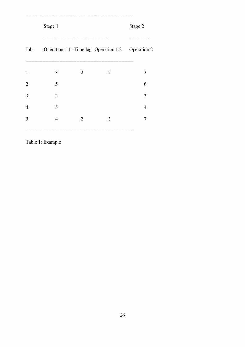
will be illustrated in the following example (table 1):

(Insert table 1 here)

For the general two-stage flow shop the algorithm of Johnson (Johnson, 1954) constructs an

8

optimal schedule. This algorithm cannot directly be applied to the example problem, as there are

7 operations to be sequenced on stage 1 and only 5 on stage 2. However, Johnson's rule can be

applied to related problems.

When we consider the related problem where the multiple operations of a job are replaced by one

operation with processing time equal to the old processing times + the time lag (e.g. processing

time of job 1 on stage 1 becomes 3+2+time lag=7), we can use Johnson's rule and get a sequence

<3,2,5,4,1> with makespan = 33. This is a feasible solution for the original problem, but not

necessarily optimal: the time lags are not productively used.

Another related problem is replacing the multiple operations by one operation with processing

time equal to the sum of the processing times of the old operations (e.g. processing time of job 1

on stage 1 becomes 3+2=5). Johnson's rule gives the sequence <3,2,5,4,1> with makespan = 30.

This is not a feasible solution for the original problem, as the restrictions concerning the time lags

are violated.

The optimal schedule has a makespan between 30 and 33. To find an optimal schedule we have to

apply an (implicit) enumerative search algorithm, as no constructive algorithm exists for this

problem.

This example has illustrated that the number of operations that have to be sequenced on a stage

can differ between the stages. Therefore, algorithms that restrict the search for an optimal

schedule to permutation schedules cannot directly be applied to this flow shop scheduling

problem. We have to apply (implicit) enumerative search algorithms to find an optimal schedule.

In the case of two stages with time lags on the first stage only, Johnson's rule can be used to

obtain a lowerbound on the makespan. In the next section we develop other lowerbounds that can

be used in the general flow shop scheduling problem with multiple operations and time lags.

9

4. LOWERBOUNDS ON THE MAKESPAN

Lowerbounds can be used to restrict the search for an optimal schedule by implicitly enumerating

subsets of schedules and deciding if it is necessary to generate schedules that belong to this

subset. If the lowerbound of this subset is smaller than the current best solution (the upperbound),

the search in the subset is continued, otherwise it is ceased.

In this section three types of lowerbounds will be developed: job based bounds, machine based

bounds and due date based bounds. These types of lowerbounds are well known from general

scheduling literature (Morton, Pentico, 1993). It is our purpose to include information on the time

lags and multiple operations in these lowerbounds, as the known lowerbounds from literature do

not make use of the inherent structure of this flow shop problem.

Before we present these lowerbounds, some more variables have to be defined:

Variables:

Pt Partial schedule with t-1 scheduled operations. The sequences B1...Bm are partially filled

with t-1 scheduled operations. 3j=1...m 3i=1...n Kij - t operations have still to be placed in

the sequences.

St Set of operations Oijk that can be added to the partial schedule Pt (e.g. Preijk belongs to

the partial schedule Pt ). Operations that belong to the set St are called schedulable

operations.

C(Pt ,j) Completion time on stage j after processing the partial schedule Pt (equal to the comple-

tion time of the last scheduled operation in the sequence Bj ).

Fijk Earliest starting time of Oijk 0 St Fijk := MAX{C(Pt ,j), C(Preijk )+Dijk }

Mijk Earliest finishing time of Oijk 0 St Mijk := Fijk +Tijk

10

4.1. Job based bounds

A job based bound determines the minimal expected completion time for the jobs. The maximum

of these completion times is a lowerbound on the makespan. It is possible to include information

on the time lags in this type of bound.

The job based lowerbound that will be presented assumes that each job starts processing on a

stage as soon as possible. The earliest finishing time of the first unscheduled operation of job i is

Mijk and this operation has to be processed on stage j. The earliest finishing time of the last

unscheduled operation of job i on this stage j is defined as LBij . After processing this operation

the job proceeds for processing on stage j+1. The earliest starting time on this stage is greater

than or equal to LBij + Dij+11, the time lag between the first operation of job i on stage j+1 and the

last operation of job i on stage j. It is possible that the completion time of the last scheduled

operation (of another job) on stage j+1, C(Pt ,j+1) is greater than the earliest starting time of the

first operation of job i on stage j+1. Therefore, we have to take the maximum of both to obtain the

earliest possible starting time of job i on stage j+1. Formally, this lowerbound can be stated as

follows:

LBjob = maxi=1...n [ LBim ] with

LBij = Mijk + 3q=k+1...Kij (Tijq+Dijq)

LBip = Max { C(Pt ,p), LBip-1+Dip1 } + Tip1 + 3q=2...Kip (Tipq+Dipq), p=j+1...m

LBip can be described as the earliest possible completion time of job i on stage p. This earliest

possible completion time is based on the partial schedule Pt .

11

4.2. Machine based bounds

It is also possible to base a lowerbound on the utilization of the different stages or machines.

Before we develop some bounds a note on the notation we use. When a bound is computed for

stage r (r=1...m) and we look at the remaining operations of a job i on this stage, there are three

possible situations:

iór Job i has no more operations to be processed on stage r: all operations Oirk , k=1...Kir

are already placed in the sequence Br ;

i0r : i0r1 The schedulable operation Oirk of job i has to be processed on stage r. Oir1...Oirk-1 are

placed in the sequence Br and Oirk ...OimKim have still to be placed in the partial

schedule.

i0r : i0r2 The schedulable operation of job i has not to be processed on stage r but on a former

stage.

The index h is used to denote the number of the first unscheduled operation of job i on stage r. If

i0r1 : h equals k, if i0r2 : h=1.

A machine based bound for stage r can be decomposed into 3 parts:

a. the earliest starting time on stage r;

b. the remaining time for processing the operations on this stage, so we get an estimation of the

earliest completion time on stage r;

c. the minimal remaining time after processing jobs on stage r.

* The earliest starting time of the first unscheduled operation of job i on stage r, EStir is: EStir=

Firk if i0r1

12

= Max { C(Pt ,r), LBir-1+Dir1 } if i0r2

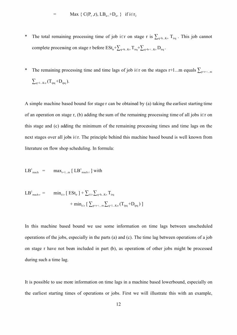
* The total remaining processing time of job i0r on stage r is 3q=h...Kir Tirq . This job cannot

complete processing on stage r before EStir+3q=h...Kir Tirq+3q=h+1...Kir Dirq .

* The remaining processing time and time lags of job i0r on the stages r+1...m equals 3p=r+1...m

3q=1...Kip (Tipq +Dipq ).

A simple machine based bound for stage r can be obtained by (a) taking the earliest starting time

of an operation on stage r, (b) adding the sum of the remaining processing time of all jobs i0r on

this stage and (c) adding the minimum of the remaining processing times and time lags on the

next stages over all jobs i0r. The principle behind this machine based bound is well known from

literature on flow shop scheduling. In formula:

LB1mach = maxr=1...m [ LB1

mach r ] with

LB1mach r = mini0r [ EStir ] + 3i0r 3q=h...Kir Tirq

+ mini0r [ 3p=r+1...m 3q=1...Kip (Tipq +Dipq ) ]

In this machine based bound we use some information on time lags between unscheduled

operations of the jobs, especially in the parts (a) and (c). The time lag between operations of a job

on stage r have not been included in part (b), as operations of other jobs might be processed

during such a time lag.

It is possible to use more information on time lags in a machine based lowerbound, especially on

the earliest starting times of operations or jobs. First we will illustrate this with an example,

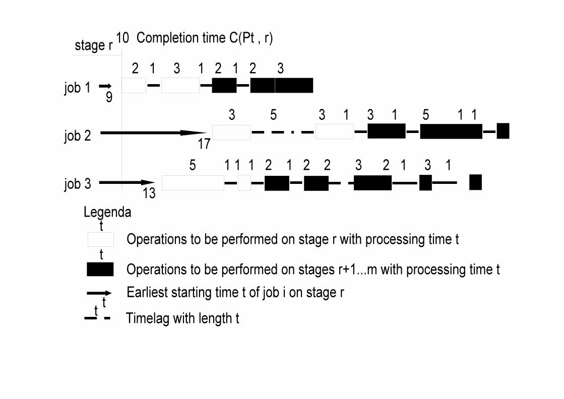
13

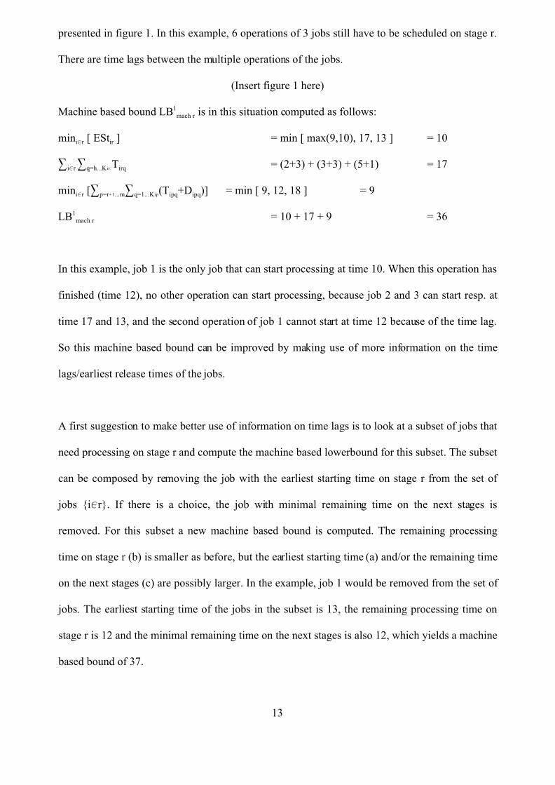
presented in figure 1. In this example, 6 operations of 3 jobs still have to be scheduled on stage r.

There are time lags between the multiple operations of the jobs.

(Insert figure 1 here)

Machine based bound LB1mach r is in this situation computed as follows:

mini0r [ EStir ] = min [ max(9,10), 17, 13 ] = 10

3i0r 3q=h...Kir Tirq = (2+3) + (3+3) + (5+1) = 17

mini0r [3p=r+1...m3q=1...Kip(Tipq+Dipq)] = min [ 9, 12, 18 ] = 9

LB1mach r = 10 + 17 + 9 = 36

In this example, job 1 is the only job that can start processing at time 10. When this operation has

finished (time 12), no other operation can start processing, because job 2 and 3 can start resp. at

time 17 and 13, and the second operation of job 1 cannot start at time 12 because of the time lag.

So this machine based bound can be improved by making use of more information on the time

lags/earliest release times of the jobs.

A first suggestion to make better use of information on time lags is to look at a subset of jobs that

need processing on stage r and compute the machine based lowerbound for this subset. The subset

can be composed by removing the job with the earliest starting time on stage r from the set of

jobs {i0r}. If there is a choice, the job with minimal remaining time on the next stages is

removed. For this subset a new machine based bound is computed. The remaining processing

time on stage r (b) is smaller as before, but the earliest starting time (a) and/or the remaining time

on the next stages (c) are possibly larger. In the example, job 1 would be removed from the set of

jobs. The earliest starting time of the jobs in the subset is 13, the remaining processing time on

stage r is 12 and the minimal remaining time on the next stages is also 12, which yields a machine

based bound of 37.

14

A second suggestion is to repeat the above mentioned construction of subsets until only one job

remains. For this job we can use all information on time lags by applying the job based bound for

this job. In the example we would remove job 3 from the subset and compute the job based bound

for job 2. This job can start at time 17, has a remaining time of 11 on stage r and 12 on the next

stages, so job 2 cannot complete before time 40.

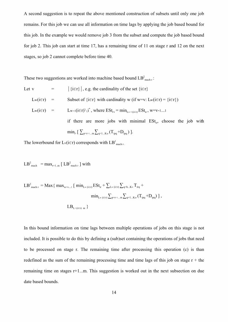
These two suggestions are worked into machine based bound LB2mach r :

Let v = *{i0r}*, e.g. the cardinality of the set {i0r}

Lw(i0r) = Subset of {i0r} with cardinality w (if w=v: Lw(i0r) = {i0r})

Lw(i0r) = Lw+1(i0r)(i* , where ESti*r = minLw+1(i0r) EStir , w=v-1...1

if there are more jobs with minimal EStir, choose the job with

mini* [ 3p=r+1...m 3q=1...Kip (Tipq +Dipq ) ].

The lowerbound for Lv(i0r) corresponds with LB1mach r .

LB2mach = maxr=1..m [ LB2

mach r ] with

LB2mach r = Max{ maxw=v...2 [ minLw (i0r) EStir + 3Lw (i0r) 3q=h...Kir Tirq +

minLw (i0r) 3p=r+1...m 3q=1...Kip (Tipq +Dipq) ] ,

LBL1 (i0r) m }

In this bound information on time lags between multiple operations of jobs on this stage is not

included. It is possible to do this by defining a (sub)set containing the operations of jobs that need

to be processed on stage r. The remaining time after processing this operation (c) is than

redefined as the sum of the remaining processing time and time lags of this job on stage r + the

remaining time on stages r+1...m. This suggestion is worked out in the next subsection on due

date based bounds.

14

The example presented has illustrated the usefulness of giving more attention to the remaining

scheduling problem on a stage when all available information on time lags is included.

4.3. Due date scheduling in determination of lowerbounds on the makespan

If we have an estimation of the makespan we can deduce from this lowerbound the latest finish

times of the jobs on stage r. With these latest finish times, which we will call artificial due dates,

for the jobs on stage r we can determine if a schedule can be constructed for stage r in which all

jobs can finish upon or before their artificial due dates. If this is not possible, we can increase the

value of the lowerbound on the makespan. This approach still generates a lowerbound on the

makespan, because it is assumed that after processing a job on stage r the processing of this job

on the next stages will not be conflicting with other jobs on these stages.

Although it is possible to use this approach for the determination of a lowerbound for each stage

r=1...m we restrict our attention to the so called bottleneck stage, that is the stage r for which the

lowerbound LBnmach r = maxp=1..m [ LBn

mach p ]. At this moment we don't make a choice which type

of machine based lowerbound we use for this approach, so n belongs to the set [1..2]. For this

stage r we try to obtain an improved lowerbound. Before we illustrate this new bound a formal

description of the artificial due dates and earliest starting times of operations on stage r is given:

DueirKir = Due date for the last operation of job i on stage r, i0r.

= LBnmach r - 3p=r+1...m 3q=1...Kip (Tipq +Dipq ) œ i0r

The due dates for the other operations of job i on this stage can now be deduced:

Dueirq-1 = Dueirq - Tirq - Dirq œ q = Kir...h+1

The earliest starting times for the operations are determined in the same way as the artificial due

dates for the operations. We introduce the symbol EStirq denoting the earliest starting time of

operation Oirq , i0r, q=h...Kir :

15

EStirh = EStir œ i0r

EStirq = EStirq-1 + Tirq-1 + Dirq œ i0r, q=h+1...Kir

Now we know for each operation that needs processing on stage r its earliest starting time and its

latest due date according to the known lowerbound on the makespan LBnmach r. What results is a

one machine scheduling problem with release dates and due dates where we are interested in

minimizing the maximal tardiness. The tardiness of an operation that can finish processing within

it's due date is zero; an operation that exceeds it's due date with an amount * has tardiness *. This

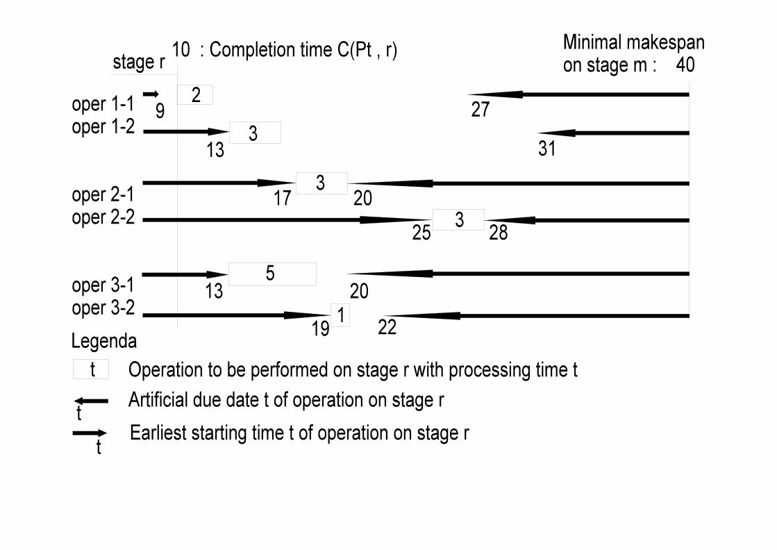
tardiness can be added to the lowerbound on the makespan that was used. We will illustrate this

in figure 2 with the same example as before:

(Insert figure 2 here)

We see that both operations of job 2 have to start exactly at their earliest starting times, otherwise

the lowerbound on the makespan cannot be reached. When the first operation of job 3 starts at

time 13, it will finish at time 18. Now we have a problem, as job 2 has to start at time 17. Because

preemption is not allowed we have to delay the start of job 3 to 20, the time at which the first

operation of job 2 has finished. Starting job 3 at time 20 gives us a new problem, as this operation

has to finish at this time. So we can conclude that the makespan of 40 cannot be reached. When

all artificial due dates are raised with one unit of time (tardiness = 1), the start of job 2, for

example, can be delayed and all other operations can be scheduled within their (new) artificial

due dates.

The idea behind a due date based bound is to determine the minimal expected tardiness of

operations on stage r. The maximum tardiness of all operations on stage r can be added to the

initial lowerbound LBnmach r. Unfortunately the resulting one machine problem is known to be NP

hard (Garey and Johnson, 1979). However, for the determination of the maximal tardiness we can

16

use a lowerbound on this tardiness.

We use subsets of the set {Oirq } and determine for these subsets the minimal necessary tardiness.

For these subsets we apply a type of preemptive scheduling to obtain a lowerbound on the

tardiness. For each subset we compute the earliest release date, add the total processing time of

the operations that belong to this subset and subtract the maximal due date of an operation in this

subset to get the expected lateness. If this lateness is greater than 0, the operations in the subset

cannot be scheduled within their artificial due dates.

The lateness can be computed for all possible combinations of operations, but this will result in

very much, and sometimes unnecessary, computations. So we decided to restrict the number of

subsets that are considered.

We observe that it is not necessary to include operations in the subset that can finish before

another operation in the subset can start. So we can construct subsets of operations whose earliest

release dates are close to each other, such that no operation in the subset can finish before another

operation in the subset can start.

If there are more operations that can start earliest at the same time, these operations can one by

one be added to the subset. If we first add the operation with the lowest artificial due date, the

resulting lateness will be highest. So, operations are added to the subset according to lowest

earliest release date, and in case of more operations with the same release date the operation with

the lowest artificial due date is added first.

We use the variable EStw to denote the earliest release date of the operation that should be added

to the subset. The wth subset that is considered, Gw (Oirq ), consists of all operations that belonged

17

to the subset Gw-1 (Oirq ) except those operations that can finish before EStw. To this subset the

operation Oirq is added that can start at EStw and has minimal artificial due date of all operations

that can start earliest at this time.

EStw = 0 w=0

= min{Oirq ó Gw-1(Oirq)} [ EStirq : EStirq $ EStw-1 ] w=1...v

RelDatew = minGw(Oirq) [ EStirq ] w=1...v

= the earliest release date of any operation from the subset Gw (Oirq ).

MaxDuew = maxGw(Oirq) [ Dueirq ] w=1...v

= the latest due date of any operation from the subset Gw (Oirq ).

Gw(Oirq) = i w=0

= Gw-1 (Oirq ) w=1...v

( { Oirq0Gw-1(Oirq ) : EStirq+Tirq <EStw }

c OirqóGw-1(Oirq ) : EStirq=EStw vDueirq =minOirq:EStirq=EStw Dueirq

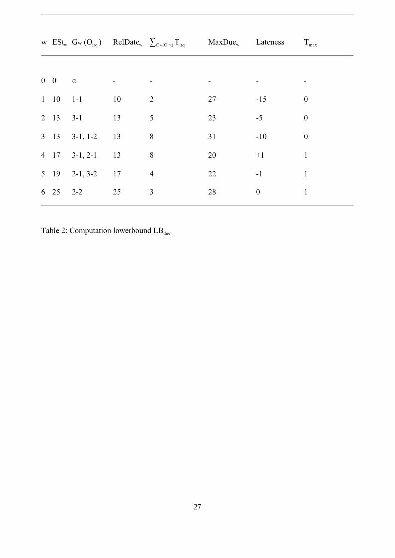
The lowerbound LBdue becomes:

LBdue = LBnmach r + Tmax , with

Tmax = MAX { 0, maxw=1...v [ RelDatew + 3Gw(Oirq) (Tirq ) - MaxDuew ] }

We will illustrate this bound with the above presented example, using LB2mach r : The initial

lowerbound on the makespan is 40. The earliest starting times and artificial due dates of the

operations are shown in figure 2. The computations are presented in table 2:

(Lateness = RelDatew + 3Gw(Oirq) (Tirq ) - MaxDuew )

(Insert table 2 here)

The maximal tardiness is 1, so the due date based bound LBdue = 40+1 = 41: the improved

lowerbound for stage r becomes 41.

18

The due date based bound that is presented uses information on time lags between multiple

operations of a job. In the experiments we use another less time consuming due date based bound.

In this bound the definition of the subset Gw (Oirq ) is changed in the set of w operations Oirq with

the smallest due dates from the total set of operations { Oirq }.

Gw (Oirq ) = Gw-1 (Oirq ) c Oirq : Dueirq =min{Oirq ó Gw-1(Oirq)}Dueirq.

At the end of this section we can conclude that it is possible to use information on time lags

between multiple operations of jobs in the development of lowerbounds on the makespan.

However, which lowerbound to use depends heavily on the complexity of the scheduling problem

(e.g. number of jobs, stages, multiple operations on a stage, variablity in processing times and

time lags, etc.) and on the branching strategy that is used in the branch and bound procedure. If,

for example, a depth first search strategy is used, it is important that the first steps in the

generation of a partial schedule are well considered, as the selection of a bad branch in the root of

the search tree causes much unnecessary computations. The lowerbounds that are developed can

be used in the selection of a branch. In the next section on heuristics we will illustrate the use of

lowerbounds for this purpose.

5. HEURISTICS AND SOME EXPERIMENTS ON THEIR PERFORMANCE

In this section suggestions are given for heuristics for this flow shop scheduling problem and

some results of experiments with these heuristics are presented.

5.1. Heuristic procedures

A heuristic procedure should generate a feasible schedule with a near-optimal makespan within

reasonable time. To generate such a schedule, the information on time lags between the multiple

operations of the jobs should be used, otherwise a non-feasible schedule could be generated.

19

Heuristics can be static or dynamic in nature. A static heuristic uses information that is known in

advance, a dynamic heuristic uses information that changes during the process of generation of

the schedule. An example of a well known static heuristic is the shortest processing time rule.

This heuristic performs generally well in job shop/flow shop scheduling.

Dynamic heuristics can be divided in heuristics that use some kind of dominance criterion to

restrict the choice between operations that can be added to the partial schedule and heuristics that

make no use of this information. The use of a dominance criterion causes more computation time,

but the results are generally better.

The next 3 dynamic heuristic do not make use of dominance criteria:

* Maximal remaining time: add to the partial schedule the schedulable operation of a job with

maximal remaining processing time and time lags in the shop. In formula: operation Oijk of

the job with maxi=1...n [ 3p=j..m 3q=h..Kip (Tipq +Dipq ) ].

* Smallest ratio: add to the partial schedule the schedulable operation of the job with the

smallest ratio of remaining processing time compared with total remaining time:

Oijk with mini=1...n [ 3p=j..m 3q=h..Kip (Tipq ) / 3p=j..m 3q=h..Kip (Tipq +Dipq ) ]. This heuristic gives

priority to operations that have relatively long time lags. When there are jobs without any

time lags, this heuristic has to be accompanied by a tie break rule.

* Largest ratio: now we add the operation with the maximum of the above mentioned expressi-

on, so operations with relatively short time lags get priority.

The next 5 heuristics that will be presented use a simple dominance criterion. The first 3

heuristics restrict their choice to operations that will generate an active schedule (a schedule

where no global left shift is possible, see e.g. (Morton, Pentico, 1993), the last 2 restrict their

20

choice to operations that will generate a non delay schedule (no unnecessary idle time added to

the schedule).

Four of these heuristics are based on a lowerbound. These heuristics compute for each schedula-

ble operation that meets the specific dominance criterion a lowerbound. The lowerbounds are

computed for the partial schedule to which this operation is added. The operation that generates a

partial schedule with minimal lowerbound is actually added to the partial schedule. In the so

called single bounds we use one type of lowerbound and compute for only one machine r with

initial lowerbound LBnmach r a due date based bound. In the combi bounds we use 2 type of bounds

and also compute these combined due date based bounds for all machines r with initial lower-

bound LBnmach r.

* Earliest completion time or minimal finish time: add to the partial schedule the schedulable

(active) operation that can finish earliest.

* Active single lowerbound: add to the partial schedule the schedulable (active) operation that

has the lowest due date based bound.

* Active combi lowerbound: when less than half of the total number of operations is placed in

the partial schedule, add to the partial schedule the schedulable (active) operation that has the

lowest due date based bound, otherwise use the less time consuming due date based bound.

* Non delay single lowerbound: equal to the active single lowerbound, except that the choice is

restricted to schedulable operations that will generate a non delay schedule.

* Non delay combi lowerbound: equal to the active combi lowerbound, except that the choice is

restricted to schedulable operations that will generate a non delay schedule.

Of these 9 heuristics, the only one that does not use any information on time lags is the shortest

processing time rule. The degree in which the other heuristics make use of this information differs

strongly. Some use only information on the time lag preceeding the schedulable operation (e.g.

21

earliest finish time), others use information on the time lags of the job to which the schedulable

operation belongs (e.g. maximal remaining time, smallest and largest ratio) or information on the

time lags of all other remaining operations (e.g. the four lowerbound heuristics).

5.2. Evaluation of heuristics

We tested the performance of these 9 heuristics for two different situations, to gain insight in the

performance of the heuristics in these special situations. In both situations 8 jobs had to be

scheduled on 4 stages. The number of operations of a job on a stage is randomly choosen and

varied between 1 and 4.

In situation I, the processing time of an operation varied between 6 and 12 time units. The time

lag before an operation was in this situation restricted to be not greater than the minimum

processing time in the shop. The minimum time lag was 2, the maximum was 6.

In situation II, more variety was allowed in processing times and time lags: both could vary

between 1 and 12 time units.

The performance of the heuristics is evaluated for 100 randomly generated test problems for both

situations. For each test problem the following measures of performance are computed:

Cmax(i,j) = Makespan for test problem i obtained by heuristic j.

Time(i,j) = Time needed for obtaining a solution for test problem i with heuristic j.

Cabs(i,j) = Deviation between makespan obtained by heuristic j and the best solution for test

problem i.

= 100% * (Cmax(i,j) - minj=1..9[Cmax(i,j)]) / minj=1..9[Cmax(i,j)]

Trel(i,j) = Relative performance of heuristic j on the computation time used to obtain the

solution for test problem i.

= (Time(i,j) - minj=1..9[Time(i,j)]) / (maxj=1..9[Time(i,j)] - minj=1..9[Time(i,j)]).

22

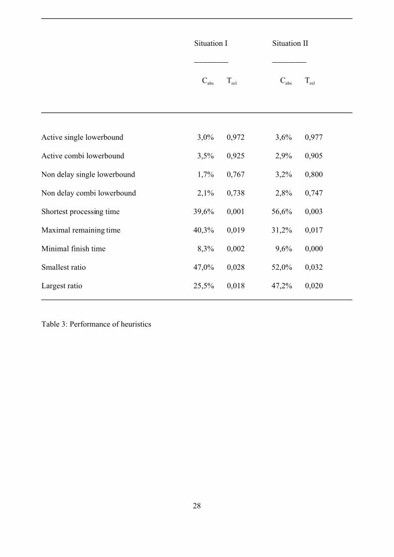
In table 3 the average Cmax performance and the average relative time performance of the nine

heuristics is presented. A relative time performance Trel near 0 means that this heuristic used on

average the least time in finding a solution. The average quality of the solutions obtained is

shown in the column Cabs. It presents the average percentage deviation between the solution

obtained by this heuristic and the best solution obtained by one of the nine heuristics.

(Insert table 3 here)

The conclusion from this table is, that the 4 heuristics that are based on lowerbounds use much

more computation time, but generate schedules with on average a lower makespan than the other

heuristics. The only heuristic with a relative makespan performance near the performance of the

lowerbound heuristics is the earliest finish time or minimal finish heuristic, that uses also a

dominance criterion in the selection of operations that can be added to the partial schedule.

The differences between situations I and II do not concern this overall conclusion. In the two

groups some shifts in relative position can be seen. For example, the maximal remaining time

heuristic performs better in situation II, where more variety in processing times and time lags was

allowed. The shortest processing time heuristic has a lower performance in this case. As this rule

makes no use of information on time lags, it could be expected that it's performance in situation II

would be lower.

The non delay lowerbound heuristics perform better than the active lowerbound heuristics. The

optimal solution need not be contained in the set of non delay schedules, but for the construction

of heuristics this dominance criterion can well be applied.

From these experiments we can conclude that in the selection of a heuristic one has to weigh the

available time for obtaining a schedule against the desired makespan performance. The lower-

bound heuristics obtain schedules with a relative low makespan, the earliest finish time heuristic

24

obtains on average in less time a schedule with a higher makespan.

6. CONCLUSIONS AND DIRECTIONS FOR FUTURE RESEARCH

In this paper we have discussed the flow shop scheduling problem with multiple operations and

time lags. The inherent structure of this flow shop can be used in the development of lower-

bounds on the makespan. Three types of lowerbounds are developed: job based bounds, machine

based bounds and due date based bounds. These lowerbounds can also be used in the construction

of heuristics for this problem. These heuristics are compared with other heuristics that use

information on time lags and multiple operations. The computational results indicate that

heuristics based on simple dominance criteria perform quite effective.

Future research on this problem has to investigate if these results are still valid in a broader range

of flow shop scheduling problems with e.g. more machines and more jobs. It should also be

investigated if there are special cases of this problem that can be solved efficiently, for example

by using specific dominance criteria. The construction and evaluation of heuristics should be

continued and broadened, as there are other promising approaches that can be applied to this

problem, e.g. tabu search, simulated annealing or genetic algorithms. Finally, research on the

second part of the hierarchical approach should be intensified.

REFERENCES

1 Aanen, E., (1988), Planning and scheduling in a flexible manufacturing system, PhD thesis,

Faculty of Mechanical Engineering, University of Twente.

2 Aanen, E., Gaalman, G.J.C., Nawijn, W.M., (1993), A scheduling approach for a flexible

manufacturing system, International Journal of Production Research, 31, 2369-2385.

3 Cao, J., Bedworth, D.D., (1992), Flow shop scheduling in serial multi-product processes with

25

transfer and set-up times, International Journal of Production Research, 30, 1819-1830.

4 Garey, M.R., Johnson, D.S., (1979), Computers and intractability: a guide to the theory of

NP-Completeness, Freeman, San Francisco.

5 Johnson, S.M., (1954), Optimal two- and three-stage production schedules with set-up times

included, Naval Research Logistics Quarterly, 1, 61-68.

6 Kern, W., Nawijn, W.M., (1991), Scheduling multi-operation jobs with time lags on a single

machine, Working paper University of Twente, Holland.

7 Mitten, L.G., (1958), Sequencing n jobs on two machines with arbitrary time lags, Manage-

ment Science, 5, 293-298.

8 Monma, C.L., (1979), The two-machine maximum flow time problem with series parallel

precedence relations: an algorithm and extension, Operations Research, 27, 792-798.

9 Morton, T.E., Pentico, D.W., (1993), Heuristic scheduling systems, with applications to

production systems and project management, John Wiley & Sons Ltd, New York.

10 Szwarc, W., (1983), Flow shop problems with time lags, Management Science, 29, 477-481.

25

Tables

26

))))))))))))))))))))))))))))))))))))))

Stage 1 Stage 2

))))))))))))))))))))))) )))))))

Job Operation 1.1 Time lag Operation 1.2 Operation 2

))))))))))))))))))))))))))))))))))))))

1 3 2 2 3

2 5 6

3 2 3

4 5 4

5 4 2 5 7

))))))))))))))))))))))))))))))))))))))

Table 1: Example

27

w EStw Gw (Oirq ) RelDatew 3Gw(Oirq) Tirq MaxDuew Lateness Tmax

0 0 i - - - - -

1 10 1-1 10 2 27 -15 0

2 13 3-1 13 5 23 -5 0

3 13 3-1, 1-2 13 8 31 -10 0

4 17 3-1, 2-1 13 8 20 +1 1

5 19 2-1, 3-2 17 4 22 -1 1

6 25 2-2 25 3 28 0 1

Table 2: Computation lowerbound LBdue

28

Situation I Situation II

)))))))Q )))))))Q

Cabs Trel Cabs Trel

Active single lowerbound 3,0% 0,972 3,6% 0,977

Active combi lowerbound 3,5% 0,925 2,9% 0,905

Non delay single lowerbound 1,7% 0,767 3,2% 0,800

Non delay combi lowerbound 2,1% 0,738 2,8% 0,747

Shortest processing time 39,6% 0,001 56,6% 0,003

Maximal remaining time 40,3% 0,019 31,2% 0,017

Minimal finish time 8,3% 0,002 9,6% 0,000

Smallest ratio 47,0% 0,028 52,0% 0,032

Largest ratio 25,5% 0,018 47,2% 0,020

Table 3: Performance of heuristics

29

List of figures

Figure 1: Example: scheduling with time lags

Figure 2: Due date based lowerbound