Flow Pattern in Horizontal and Vertical Tubes

8/14/2019 Flow Pattern in Horizontal and Vertical Tubes

http://slidepdf.com/reader/full/flow-pattern-in-horizontal-and-vertical-tubes 1/34

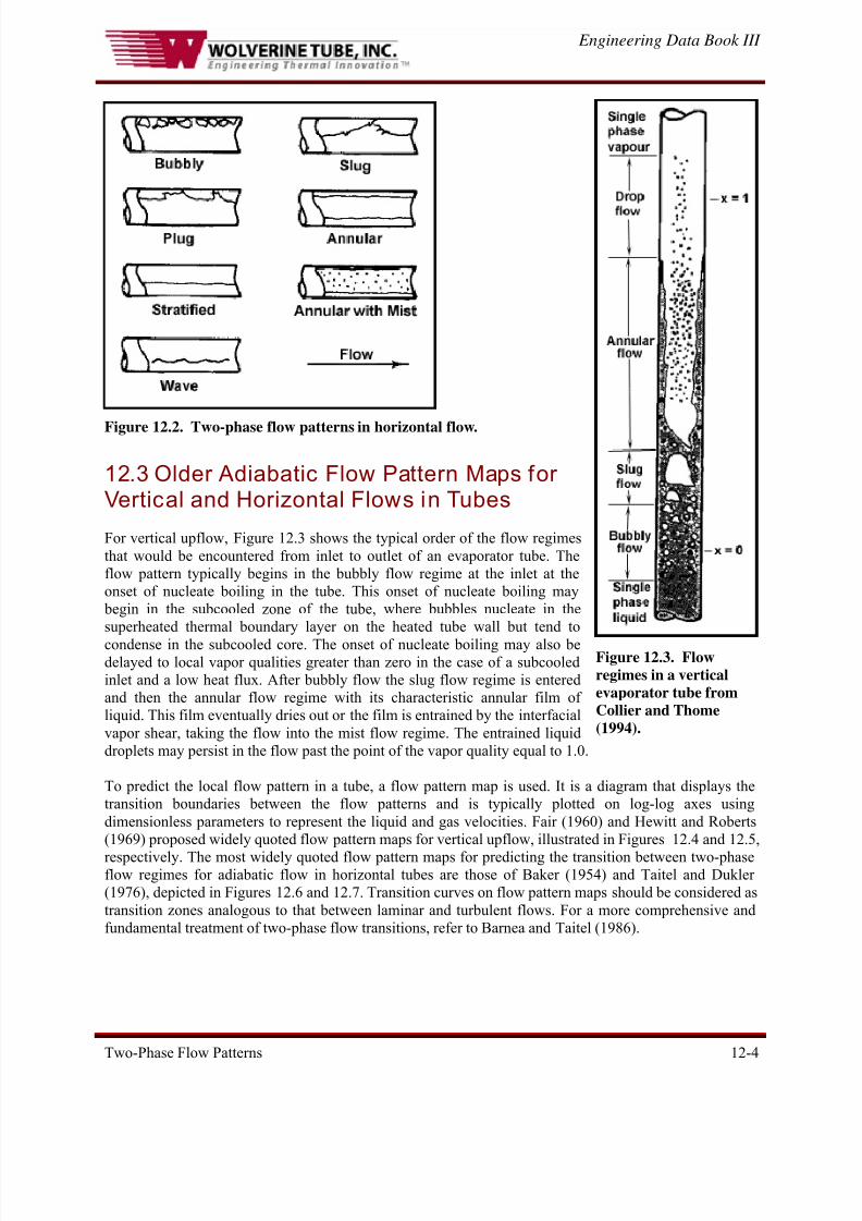
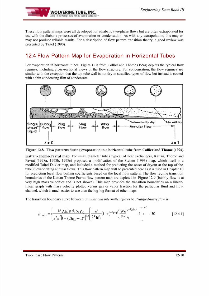
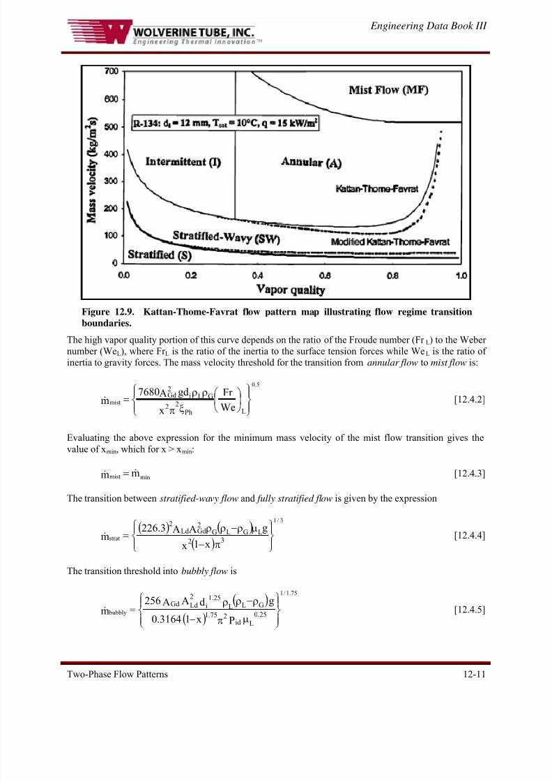
Engineering Data Book III

Two-Phase Flow Patterns 12-1

Chapter 12

Two-Phase Flow Patterns

(This chapter was updated in 2007)

SUMMARY: For two-phase flows, the respective distribution of the liquid and vapor phases in the flow

channel is an important aspect of their description. Their respective distributions take on some commonly

observed flow structures, which are defined as two-phase flow patterns that have particular identifying

characteristics. Heat transfer coefficients and pressure drops are closely related to the local two-phase

flow structure of the fluid, and thus two-phase flow pattern prediction is an important aspect of modeling

evaporation and condensation. In fact, recent heat transfer models for predicting intube boiling and

condensation are based on the local flow pattern and hence, by necessity, require reliable flow pattern

maps to identify what type of flow pattern exists at the local flow conditions. Analogous to predicting the

transition from laminar to turbulent flow in single-phase flows, two-phase flow pattern maps are used for

predicting the transition from one type of two-phase flow pattern to another.

In this chapter, first the geometric characteristics of flow patterns inside tubes will be described for

vertical upward and horizontal flows. Next, several of the widely quoted, older flow pattern maps for

vertical and horizontal flows will be presented. Then, a recent flow pattern map and its flow regime

transition equations specifically for adiabatic flows and in particular for evaporation and condensation in

horizontal tubes will be presented. Finally, flow patterns in two-phase flows over tube bundles will be

addressed and a flow pattern map proposed for those flows will be shown.

12.1 Flow Patterns in Vertical Tubes

For co-current upflow of gas and liquid in a vertical tube, the liquid and gas phases distribute themselves

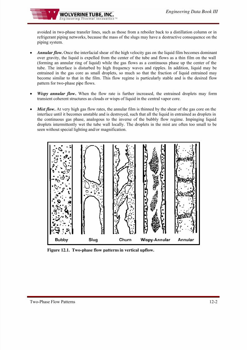
into several recognizable flow structures. These are referred to as flow patterns and they are depicted inFigure 12.1 and can be described as follows:

• Bubbly flow. Numerous bubbles are observable as the gas is dispersed in the form of discrete bubbles

in the continuous liquid phase. The bubbles may vary widely in size and shape but they are typically

nearly spherical and are much smaller than the diameter of the tube itself.

• Slug flow. With increasing gas void fraction, the proximity of the bubbles is very close such that

bubbles collide and coalesce to form larger bubbles, which are similar in dimension to the tube

diameter. These bubbles have a characteristic shape similar to a bullet with a hemispherical nose with

a blunt tail end. They are commonly referred to as Taylor bubbles after the instability of that name.

Taylor bubbles are separated from one another by slugs of liquid, which may include small bubbles.

Taylor bubbles are surrounded by a thin liquid film between them and the tube wall, which may flowdownward due to the force of gravity, even though the net flow of fluid is upward.

• Churn flow. Increasing the velocity of the flow, the structure of the flow becomes unstable with the

fluid traveling up and down in an oscillatory fashion but with a net upward flow. The instability is the

result of the relative parity of the gravity and shear forces acting in opposing directions on the thin

film of liquid of Taylor bubbles. This flow pattern is in fact an intermediate regime between the slug

flow and annular flow regimes. In small diameter tubes, churn flow may not develop at all and the

flow passes directly from slug flow to annular flow. Churn flow is typically a flow regime to be





avoided in two-phase transfer lines, such as those from a reboiler back to a distillation column or in

refrigerant piping networks, because the mass of the slugs may have a destructive consequence on the

piping system.

• Annular flow. Once the interfacial shear of the high velocity gas on the liquid film becomes dominant

over gravity, the liquid is expelled from the center of the tube and flows as a thin film on the wall

(forming an annular ring of liquid) while the gas flows as a continuous phase up the center of thetube. The interface is disturbed by high frequency waves and ripples. In addition, liquid may be

entrained in the gas core as small droplets, so much so that the fraction of liquid entrained may

become similar to that in the film. This flow regime is particularly stable and is the desired flow

pattern for two-phase pipe flows.

• Wispy annular flow. When the flow rate is further increased, the entrained droplets may form

transient coherent structures as clouds or wisps of liquid in the central vapor core.

• Mist flow. At very high gas flow rates, the annular film is thinned by the shear of the gas core on the

interface until it becomes unstable and is destroyed, such that all the liquid in entrained as droplets in

the continuous gas phase, analogous to the inverse of the bubbly flow regime. Impinging liquid

droplets intermittently wet the tube wall locally. The droplets in the mist are often too small to be

seen without special lighting and/or magnification.

Figure 12.1. Two-phase flow patterns in vertical upflow.





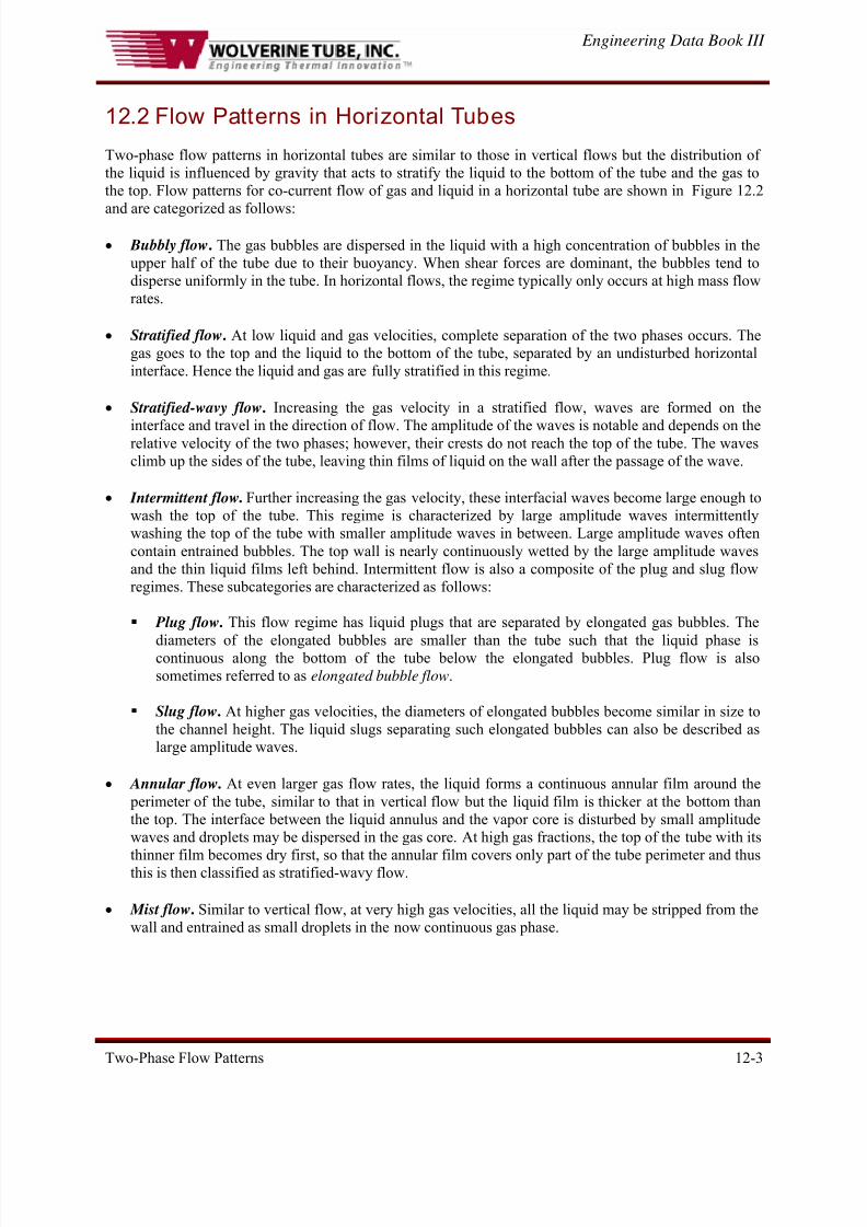
12.2 Flow Patterns in Horizontal Tubes

Two-phase flow patterns in horizontal tubes are similar to those in vertical flows but the distribution of

the liquid is influenced by gravity that acts to stratify the liquid to the bottom of the tube and the gas to

the top. Flow patterns for co-current flow of gas and liquid in a horizontal tube are shown in Figure 12.2

and are categorized as follows:

• Bubbly flow. The gas bubbles are dispersed in the liquid with a high concentration of bubbles in the

upper half of the tube due to their buoyancy. When shear forces are dominant, the bubbles tend to

disperse uniformly in the tube. In horizontal flows, the regime typically only occurs at high mass flow

rates.

• Stratified flow. At low liquid and gas velocities, complete separation of the two phases occurs. The

gas goes to the top and the liquid to the bottom of the tube, separated by an undisturbed horizontal

interface. Hence the liquid and gas are fully stratified in this regime.

• Stratified-wavy flow. Increasing the gas velocity in a stratified flow, waves are formed on the

interface and travel in the direction of flow. The amplitude of the waves is notable and depends on therelative velocity of the two phases; however, their crests do not reach the top of the tube. The waves

climb up the sides of the tube, leaving thin films of liquid on the wall after the passage of the wave.

• Intermittent flow. Further increasing the gas velocity, these interfacial waves become large enough to

wash the top of the tube. This regime is characterized by large amplitude waves intermittently

washing the top of the tube with smaller amplitude waves in between. Large amplitude waves often

contain entrained bubbles. The top wall is nearly continuously wetted by the large amplitude waves

and the thin liquid films left behind. Intermittent flow is also a composite of the plug and slug flow

regimes. These subcategories are characterized as follows:

Plug flow. This flow regime has liquid plugs that are separated by elongated gas bubbles. The

diameters of the elongated bubbles are smaller than the tube such that the liquid phase iscontinuous along the bottom of the tube below the elongated bubbles. Plug flow is also

sometimes referred to as elongated bubble flow.

Slug flow. At higher gas velocities, the diameters of elongated bubbles become similar in size to

the channel height. The liquid slugs separating such elongated bubbles can also be described as

large amplitude waves.

• Annular flow. At even larger gas flow rates, the liquid forms a continuous annular film around the

perimeter of the tube, similar to that in vertical flow but the liquid film is thicker at the bottom than

the top. The interface between the liquid annulus and the vapor core is disturbed by small amplitude

waves and droplets may be dispersed in the gas core. At high gas fractions, the top of the tube with its

thinner film becomes dry first, so that the annular film covers only part of the tube perimeter and thusthis is then classified as stratified-wavy flow.

• Mist flow. Similar to vertical flow, at very high gas velocities, all the liquid may be stripped from the

wall and entrained as small droplets in the now continuous gas phase.







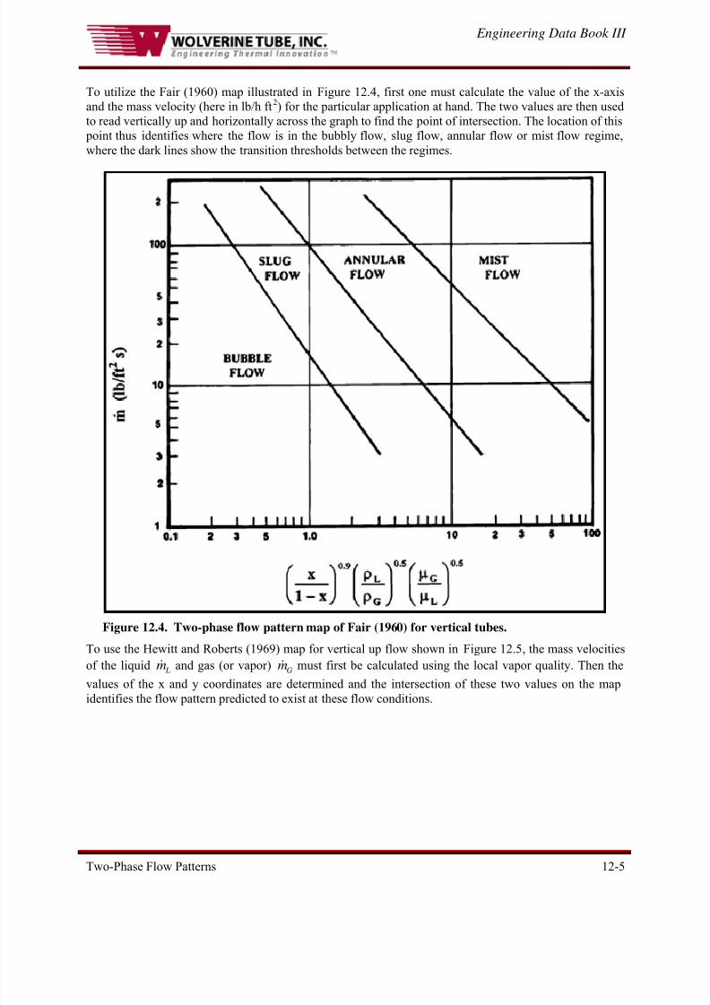
To utilize the Fair (1960) map illustrated in Figure 12.4, first one must calculate the value of the x-axis

and the mass velocity (here in lb/h ft2) for the particular application at hand. The two values are then used

to read vertically up and horizontally across the graph to find the point of intersection. The location of this

point thus identifies where the flow is in the bubbly flow, slug flow, annular flow or mist flow regime,

where the dark lines show the transition thresholds between the regimes.

Figure 12.4. Two-phase flow pattern map of Fair (1960) for vertical tubes.

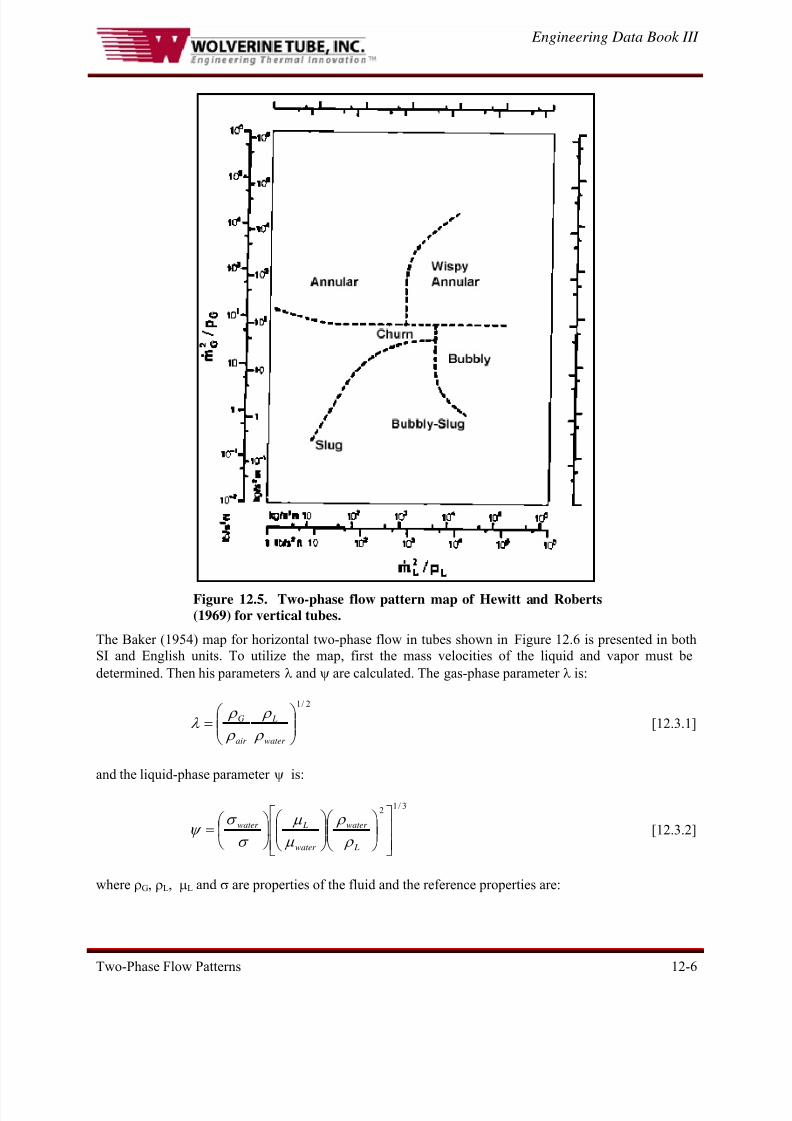
To use the Hewitt and Roberts (1969) map for vertical up flow shown in Figure 12.5, the mass velocities

of the liquid and gas (or vapor) must first be calculated using the local vapor quality. Then the

values of the x and y coordinates are determined and the intersection of these two values on the map

identifies the flow pattern predicted to exist at these flow conditions.

Lm& Gm&





Figure 12.5. Two-phase flow pattern map of Hewitt and Roberts(1969) for vertical tubes.

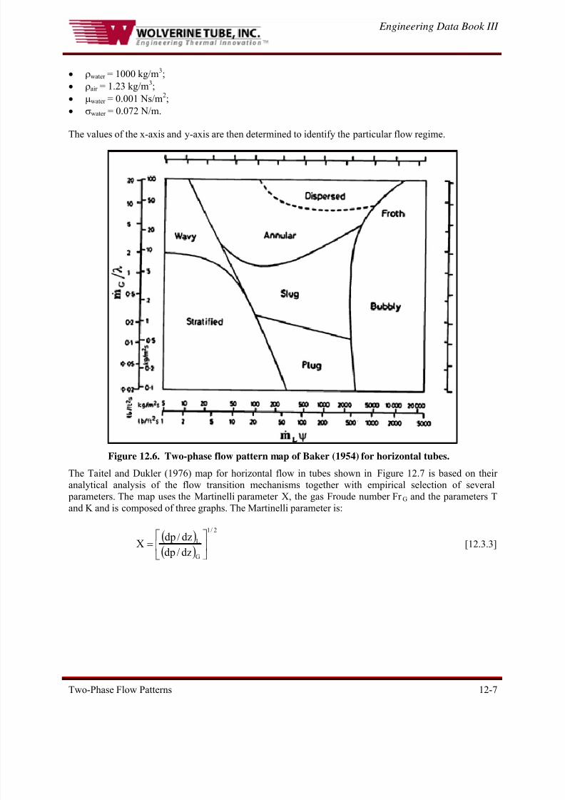
The Baker (1954) map for horizontal two-phase flow in tubes shown in Figure 12.6 is presented in both

SI and English units. To utilize the map, first the mass velocities of the liquid and vapor must be

determined. Then his parameters λ and ψ are calculated. The gas-phase parameter λ is:

2/1

⎟⎟ ⎠

⎞⎜⎜⎝

⎛ =

water

L

air

G

ρ

ρ

ρ

ρ λ

[12.3.1]

and the liquid-phase parameter ψ is:

3/12

⎥⎥⎦

⎤

⎢⎢⎣

⎡⎟⎟ ⎠

⎞⎜⎜⎝

⎛ ⎟⎟ ⎠

⎞⎜⎜⎝

⎛ ⎟ ⎠

⎞⎜⎝

⎛ =

L

water

water

Lwater

ρ

ρ

μ

μ

σ

σ ψ

[12.3.2]

where ρG, ρL, μL and σ are properties of the fluid and the reference properties are:





• ρwater = 1000 kg/m3;

• ρair = 1.23 kg/m3;

• μwater = 0.001 Ns/m2;

• σwater = 0.072 N/m.

The values of the x-axis and y-axis are then determined to identify the particular flow regime.

Figure 12.6. Two-phase flow pattern map of Baker (1954) for horizontal tubes.

The Taitel and Dukler (1976) map for horizontal flow in tubes shown in Figure 12.7 is based on their

analytical analysis of the flow transition mechanisms together with empirical selection of several

parameters. The map uses the Martinelli parameter X, the gas Froude number Fr G and the parameters T

and K and is composed of three graphs. The Martinelli parameter is:

( )( )

2/1

G

L

dz/dp

dz/dpX ⎥

⎦

⎤⎢

⎣

⎡=

[12.3.3]





Figure 12.7. Two-phase flow pattern map of Taitel and Dukler (1976) for horizontaltubes.





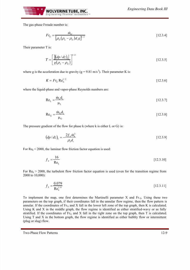
The gas-phase Froude number is:

( )[ ] 2/1gd

mFr

iG LG

GG

ρ ρ ρ −=

&

[12.3.4]

Their parameter T is:

( )( )

2/1

/⎥⎦

⎤⎢⎣

⎡

−=

G L

L

g

dzdpT

ρ ρ

[12.3.5]

where g is the acceleration due to gravity (g = 9.81 m/s2). Their parameter K is:

[12.3.6]2/1Re LGFr K =

where the liquid-phase and vapor-phase Reynolds numbers are:

L

iLL

dmRe

μ=

&

[12.3.7]

G

iGG

dmRe

μ=

&

[12.3.8]

The pressure gradient of the flow for phase k (where k is either L or G) is:

( )ik

k k k

d

mdzdp

ρ

22/

&ƒ−=

[12.3.9]

For Rek < 2000, the laminar flow friction factor equation is used:

k

k Re

16=ƒ

[12.3.10]

For Rek > 2000, the turbulent flow friction factor equation is used (even for the transition regime from

2000 to 10,000):

4/1

Re

079.0

k

k =ƒ

[12.3.11]

To implement the map, one first determines the Martinelli parameter X and Fr G. Using these two

parameters on the top graph, if their coordinates fall in the annular flow regime, then the flow pattern is

annular. If the coordinates of Fr G and X fall in the lower left zone of the top graph, then K is calculated.

Using K and X in the middle graph, the flow regime is identified as either stratified-wavy or as fully

stratified. If the coordinates of Fr G and X fall in the right zone on the top graph, then T is calculated.

Using T and X in the bottom graph, the flow regime is identified as either bubbly flow or intermittent(plug or slug) flow.









In the above equations, the ratio of We to Fr is

L

i LWe

Fr

g d⎛ ⎝ ⎜

⎞ ⎠⎟ =

2 ρ

σ

[12.4.6]

and the friction factor is

2

Ld

PhA5.1

log2138.1

−

⎥⎦

⎤⎢⎣

⎡⎟⎟ ⎠

⎞⎜⎜⎝

⎛ π+=ξ

[12.4.7]

The non-dimensional empirical exponents F1(q) and F2(q) in the boundary equation include the

effect of heat flux on the onset of dryout of the annular film, i.e. the transition of annular flow into

annular flow with partial dryout, the latter which is classified as stratified-wavy flow by the map. They

are:

wavym&

⎟⎟ ⎠

⎞⎜⎜⎝

⎛ +⎟

⎟ ⎠

⎞⎜⎜⎝

⎛ =

q

q8.64

q

q0.646)q(F

DNBDNB

2

1

[12.4.8a]

023.1q

q8.18)q(F

DNB

2 +⎟⎟ ⎠

⎞⎜⎜⎝

⎛ =

[12.4.8b]

The Kutateladze (1948) correlation for the heat flux of departure from nucleate boiling, qDNB is used tonormalize the local heat flux:

[12.4.9]( )[ ]σρ−ρρ= GL

4/1LGG

2/1

DNB gh131.0q

The vertical boundary between intermittent flow and annular flow is assumed to occur at a fixed value of

the Martinelli parameter, Xtt, equal to 0.34, where Xtt is defined as:

⎟⎟ ⎠

⎞⎜⎜⎝

⎛

μ

μ⎟⎟ ⎠

⎞⎜⎜⎝

⎛

ρ

ρ⎟ ⎠

⎞⎜⎝

⎛ −=

G

L

L

G

125.05.0875.0

ttx

x1X

[12.4.10]

Solving for x, the threshold line of the intermittent-to-annular flow transition at xIA is:

⎪⎭

⎪⎬⎫

⎪⎩

⎪⎨⎧ +

⎥⎥

⎦

⎤⎢⎢

⎣

⎡⎟⎟ ⎠

⎞⎜⎜⎝

⎛ μμ

⎟⎟ ⎠

⎞⎜⎜⎝

⎛ ρρ=

−−

−

12914.0xG

L7/1

L

G75.1/1

1

IA

[12.4.11]





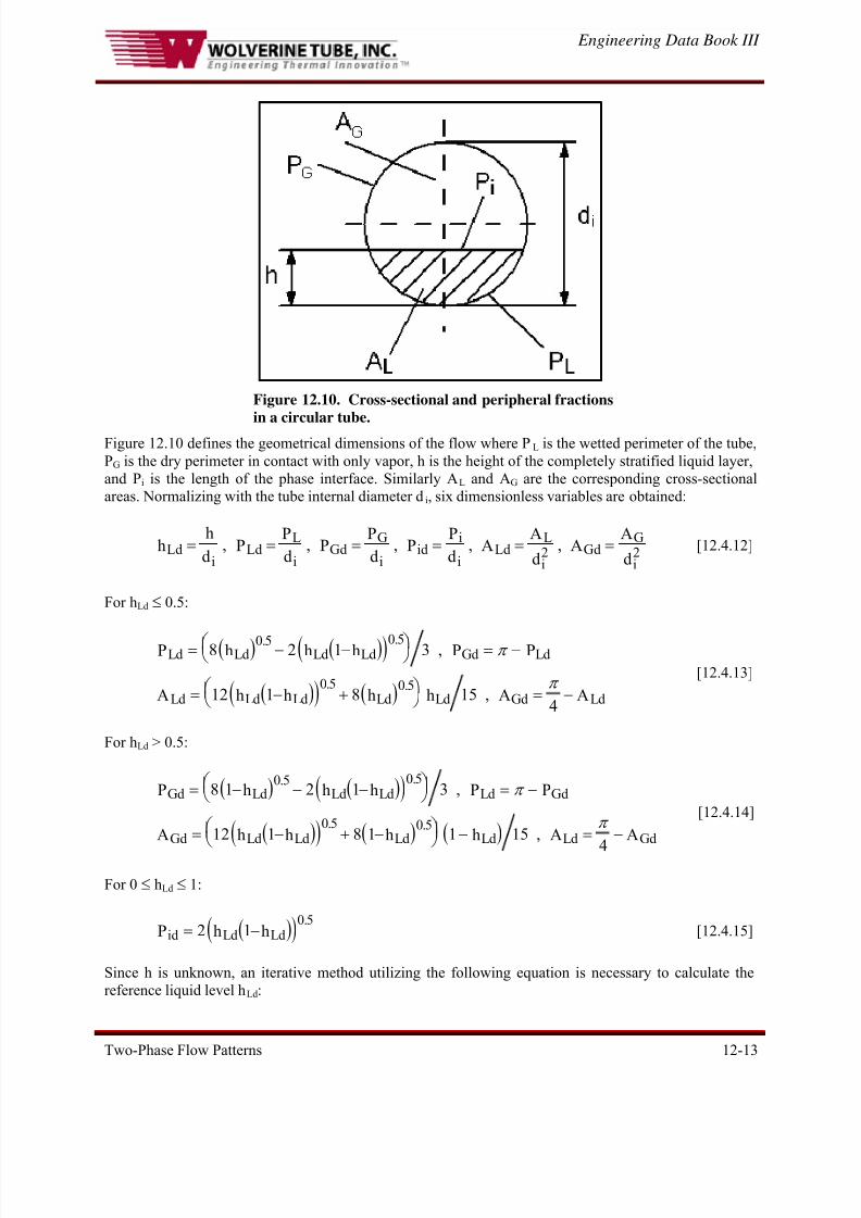
Figure 12.10. Cross-sectional and peripheral fractionsin a circular tube.

Figure 12.10 defines the geometrical dimensions of the flow where PL is the wetted perimeter of the tube,

PG is the dry perimeter in contact with only vapor, h is the height of the completely stratified liquid layer,

and Pi is the length of the phase interface. Similarly AL and AG are the corresponding cross-sectional

areas. Normalizing with the tube internal diameter di, six dimensionless variables are obtained:

Ldi

LdL

iGd

G

iid

i

iLd

L

iGd

G

i

hh

dP

P

dP

P

dP

P

dA

A

dA

A

d= = = = = =, , , , ,

2 2

[12.4.12]

For hLd ≤ 0.5:

( ) ( )( )

( )( ) ( )

Ld Ld Ld Ld Gd Ld

Ld Ld Ld Ld Ld Gd Ld

P h h h P P

A h h h h A

= − −⎛ ⎝ ⎜ ⎞ ⎠⎟ = −

= − +⎛ ⎝ ⎜ ⎞

⎠⎟ = −

8 2 1 3

12 1 8 154

0 5 0 5

0 5 0 5

. .

. .

,

,

π

π A

[12.4.13]

For hLd > 0.5:

( ) ( )( )

( )( ) ( ) ( )

Gd Ld Ld Ld Ld Gd

Gd Ld Ld Ld Ld Ld Gd

P h h h P P

A h h h h A

= − − −⎛ ⎝ ⎜ ⎞

⎠⎟ = −

= − + −⎛ ⎝ ⎜ ⎞

⎠⎟ − =

8 1 2 1 3

12 1 8 1 1 15

4

0 5 0 5

0 5 0 5

. .

. .

,

,

π

π A−

[12.4.14]

For 0 ≤ hLd ≤ 1:

[12.4.15]( )( )id Ld LdP h h= −2 10 5.

Since h is unknown, an iterative method utilizing the following equation is necessary to calculate the

reference liquid level hLd:





ttGd id

Gd

Gd id

Gd

id

Ld Ld

Ld

LdX

P P

A

P P

A

P

A P

A

P2

1 4 2

2

1 4 3

264

64=

+⎛ ⎝ ⎜

⎞ ⎠⎟

⎛

⎝ ⎜

⎞

⎠⎟

++

⎛

⎝ ⎜

⎞

⎠⎟

⎡

⎣⎢⎢

⎤

⎦⎥⎥

⎛

⎝ ⎜

⎞

⎠⎟

⎛

⎝ ⎜

⎞

⎠⎟

π

π π

π

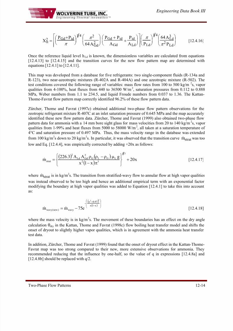
[12.4.16]

Once the reference liquid level hLd is known, the dimensionless variables are calculated from equations[12.4.13] to [12.4.15] and the transition curves for the new flow pattern map are determined with

equations [12.4.1] to [12.4.11].

This map was developed from a database for five refrigerants: two single-component fluids (R-134a and

R-123), two near-azeotropic mixtures (R-402A and R-404A) and one azeotropic mixture (R-502). The

test conditions covered the following range of variables: mass flow rates from 100 to 500 kg/m 2s, vapor

qualities from 4-100%, heat fluxes from 440 to 36500 W/m2, saturation pressures from 0.112 to 0.888

MPa, Weber numbers from 1.1 to 234.5, and liquid Froude numbers from 0.037 to 1.36. The Kattan-

Thome-Favrat flow pattern map correctly identified 96.2% of these flow pattern data.

Zürcher, Thome and Favrat (1997c) obtained additional two-phase flow pattern observations for the

zeotropic refrigerant mixture R-407C at an inlet saturation pressure of 0.645 MPa and the map accurately

identified these new flow pattern data. Zürcher, Thome and Favrat (1999) also obtained two-phase flow

pattern data for ammonia with a 14 mm bore sight glass for mass velocities from 20 to 140 kg/m2s, vapor

qualities from 1-99% and heat fluxes from 5000 to 58000 W/m2, all taken at a saturation temperature of

4°C and saturation pressure of 0.497 MPa. Thus, the mass velocity range in the database was extended

from 100 kg/m2s down to 20 kg/m2s. In particular, it was observed that the transition curve was too

low and Eq. [12.4.4], was empirically corrected by adding +20x as follows:

stratm&

( ) ( )( )

x20x1x

gAA3.226m

31

32

LGLG

2

GdLd

2

strat +⎭⎬⎫

⎩⎨⎧

π−μρ−ρρ

=&

[12.4.17]

where is in kg/mstratm&2s. The transition from stratified-wavy flow to annular flow at high vapor qualities

was instead observed to be too high and hence an additional empirical term with an exponential factor

modifying the boundary at high vapor qualities was added to Equation [12.4.1] to take this into account

as:

( )( ) ⎟

⎟

⎠

⎞

⎜⎜

⎝

⎛

−

−−

−=x1x

97.0x

wavy)new(wavy

22

e75mm &&

[12.4.18]

where the mass velocity is in kg/m2s. The movement of these boundaries has an effect on the dry angle

calculation θdry in the Kattan, Thome and Favrat (1998c) flow boiling heat transfer model and shifts the

onset of dryout to slightly higher vapor qualities, which is in agreement with the ammonia heat transfertest data.

In addition, Zürcher, Thome and Favrat (1999) found that the onset of dryout effect in the Kattan-Thome-

Favrat map was too strong compared to their new, more extensive observations for ammonia. They

recommended reducing that the influence by one-half, so the value of q in expressions [12.4.8a] and

[12.4.8b] should be replaced with q/2.





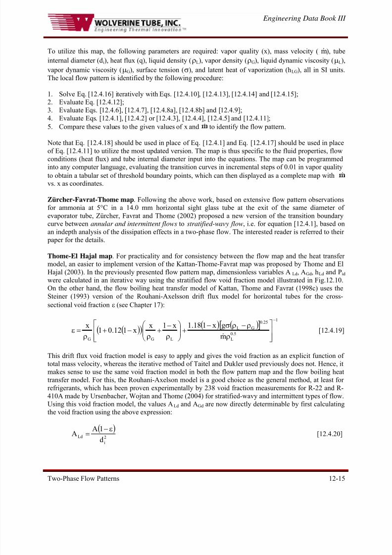
To utilize this map, the following parameters are required: vapor quality (x), mass velocity ( m& ), tube

internal diameter (di), heat flux (q), liquid density (ρL), vapor density (ρG), liquid dynamic viscosity (μL),

vapor dynamic viscosity (μG), surface tension (σ), and latent heat of vaporization (hLG), all in SI units.

The local flow pattern is identified by the following procedure:

1. Solve Eq. [12.4.16] iteratively with Eqs. [12.4.10], [12.4.13], [12.4.14] and [12.4.15];2. Evaluate Eq. [12.4.12];

3. Evaluate Eqs. [12.4.6], [12.4.7], [12.4.8a], [12.4.8b] and [12.4.9];

4. Evaluate Eqs. [12.4.1], [12.4.2] or [12.4.3], [12.4.4], [12.4.5] and [12.4.11];

5. Compare these values to the given values of x and & to identify the flow pattern.

Note that Eq. [12.4.18] should be used in place of Eq. [12.4.1] and Eq. [12.4.17] should be used in place

of Eq. [12.4.11] to utilize the most updated version. The map is thus specific to the fluid properties, flow

conditions (heat flux) and tube internal diameter input into the equations. The map can be programmed

into any computer language, evaluating the transition curves in incremental steps of 0.01 in vapor quality

to obtain a tabular set of threshold boundary points, which can then displayed as a complete map with & vs. x as coordinates.

Zürcher-Favrat-Thome map. Following the above work, based on extensive flow pattern observations

for ammonia at 5°C in a 14.0 mm horizontal sight glass tube at the exit of the same diameter of

evaporator tube, Zürcher, Favrat and Thome (2002) proposed a new version of the transition boundarycurve between annular and intermittent flows to stratified-wavy flow, i.e. for equation [12.4.1], based on

an indepth analysis of the dissipation effects in a two-phase flow. The interested reader is referred to their

paper for the details.

Thome-El Hajal map. For practicality and for consistency between the flow map and the heat transfermodel, an easier to implement version of the Kattan-Thome-Favrat map was proposed by Thome and El

Hajal (2003). In the previously presented flow pattern map, dimensionless variables ALd, AGd, hLd and Pid

were calculated in an iterative way using the stratified flow void fraction model illustrated in Fig.12.10.

On the other hand, the flow boiling heat transfer model of Kattan, Thome and Favrat (1998c) uses theSteiner (1993) version of the Rouhani-Axelsson drift flux model for horizontal tubes for the cross-

sectional void fraction ε (see Chapter 17):

( )( ) ( ) ( )[ ]

1

5.0

L

25.0

GL

LGG m

gx118.1x1xx112.01

x−

⎥⎥⎦

⎤

⎢⎢⎣

⎡

ρ

ρ−ρσ−+⎟⎟

⎠

⎞⎜⎜⎝

⎛

ρ−

+ρ

−+ρ

=ε&

[12.4.19]

This drift flux void fraction model is easy to apply and gives the void fraction as an explicit function of

total mass velocity, whereas the iterative method of Taitel and Dukler used previously does not. Hence, it

makes sense to use the same void fraction model in both the flow pattern map and the flow boiling heat

transfer model. For this, the Rouhani-Axelson model is a good choice as the general method, at least for

refrigerants, which has been proven experimentally by 238 void fraction measurements for R-22 and R-410A made by Ursenbacher, Wojtan and Thome (2004) for stratified-wavy and intermittent types of flow.

Using this void fraction model, the values ALd and AGd are now directly determinable by first calculating

the void fraction using the above expression:

( )2

i

Ldd

1AA

ε−= [12.4.20]





2

i

Gdd

AA

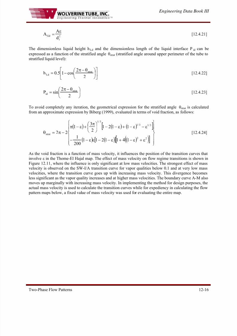
ε= [12.4.21]

The dimensionless liquid height hLd and the dimensionless length of the liquid interface P id can be

expressed as a function of the stratified angle θstrat (stratified angle around upper perimeter of the tube to

stratified liquid level):

⎥⎦

⎤⎢⎣

⎡⎟ ⎠

⎞⎜⎝

⎛ θ−π−=

2

2cos15.0h strat

Ld [12.4.22]

⎟ ⎠

⎞⎜⎝

⎛ θ−π=

2

2sinP strat

id [12.4.23]

To avoid completely any iteration, the geometrical expression for the stratified angle θstrat is calculated

from an approximate expression by Biberg (1999), evaluated in terms of void fraction, as follows:

( ) ( ) ( )[ ]

( ) ( )[ ] ( )( )[ ] ⎪⎪⎭

⎪⎪⎬

⎫

⎪⎪⎩

⎪⎪⎨

⎧

ε+ε−+ε−−εε−−

ε−ε−+ε−−⎟ ⎠

⎞⎜⎝

⎛ π+ε−π

−π=θ22

3/13/1

3/1

strat

1411211200

1

11212

31

22 [12.4.24]

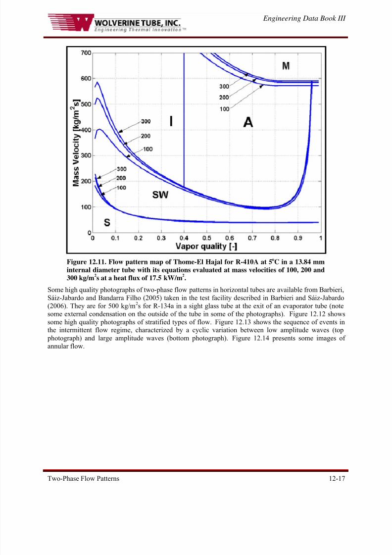
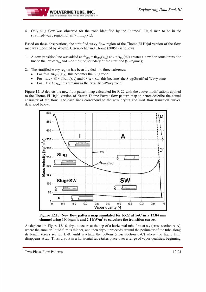
As the void fraction is a function of mass velocity, it influences the position of the transition curves that

involve ε in the Thome-El Hajal map. The effect of mass velocity on flow regime transitions is shown in

Figure 12.11, where the influence is only significant at low mass velocities. The strongest effect of massvelocity is observed on the SW-I/A transition curve for vapor qualities below 0.1 and at very low mass

velocities, where the transition curve goes up with increasing mass velocity. This divergence becomes

less significant as the vapor quality increases and at higher mass velocities. The boundary curve A-M alsomoves up marginally with increasing mass velocity. In implementing the method for design purposes, the

actual mass velocity is used to calculate the transition curves while for expediency in calculating the flow

pattern maps below, a fixed value of mass velocity was used for evaluating the entire map.





Figure 12.11. Flow pattern map of Thome-El Hajal for R-410A at 5oC in a 13.84 mminternal diameter tube with its equations evaluated at mass velocities of 100, 200 and300 kg/m2s at a heat flux of 17.5 kW/m2.

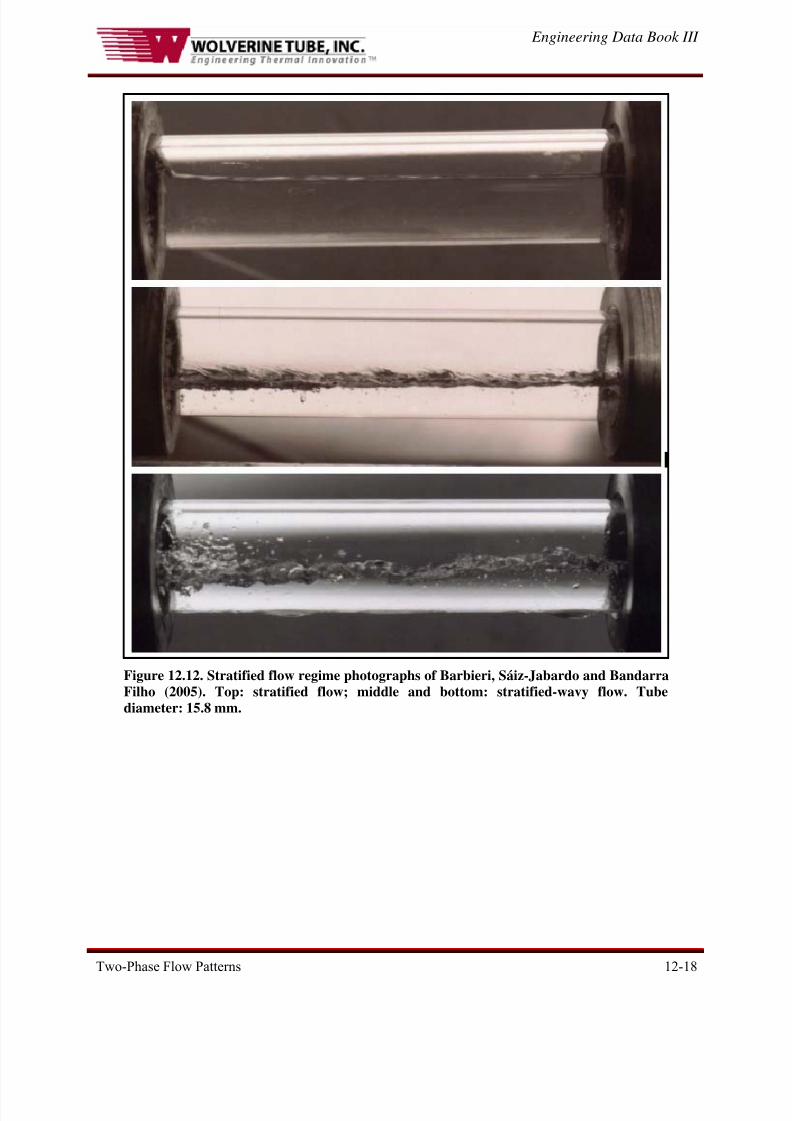
Some high quality photographs of two-phase flow patterns in horizontal tubes are available from Barbieri,Sáiz-Jabardo and Bandarra Filho (2005) taken in the test facility described in Barbieri and Sáiz-Jabardo

(2006). They are for 500 kg/m2s for R-134a in a sight glass tube at the exit of an evaporator tube (note

some external condensation on the outside of the tube in some of the photographs). Figure 12.12 shows

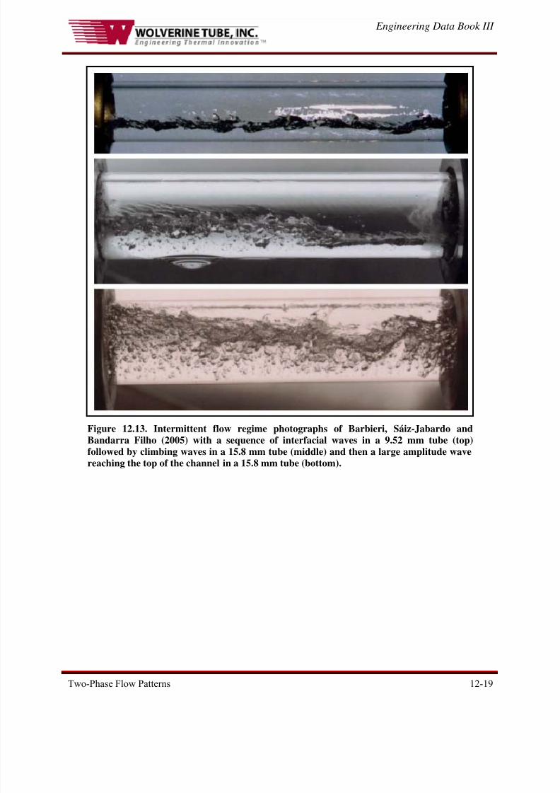
some high quality photographs of stratified types of flow. Figure 12.13 shows the sequence of events inthe intermittent flow regime, characterized by a cyclic variation between low amplitude waves (top

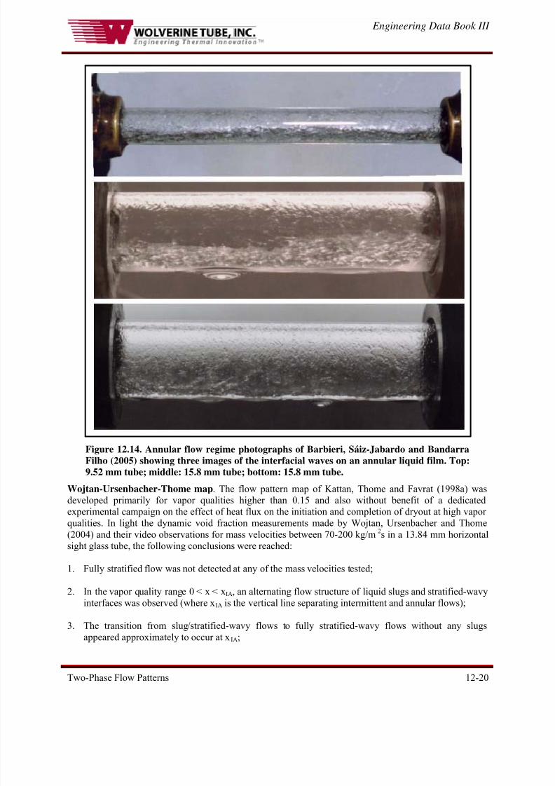
photograph) and large amplitude waves (bottom photograph). Figure 12.14 presents some images of

annular flow.





Figure 12.12. Stratified flow regime photographs of Barbieri, Sáiz-Jabardo and BandarraFilho (2005). Top: stratified flow; middle and bottom: stratified-wavy flow. Tubediameter: 15.8 mm.





Figure 12.13. Intermittent flow regime photographs of Barbieri, Sáiz-Jabardo andBandarra Filho (2005) with a sequence of interfacial waves in a 9.52 mm tube (top)followed by climbing waves in a 15.8 mm tube (middle) and then a large amplitude wavereaching the top of the channel in a 15.8 mm tube (bottom).









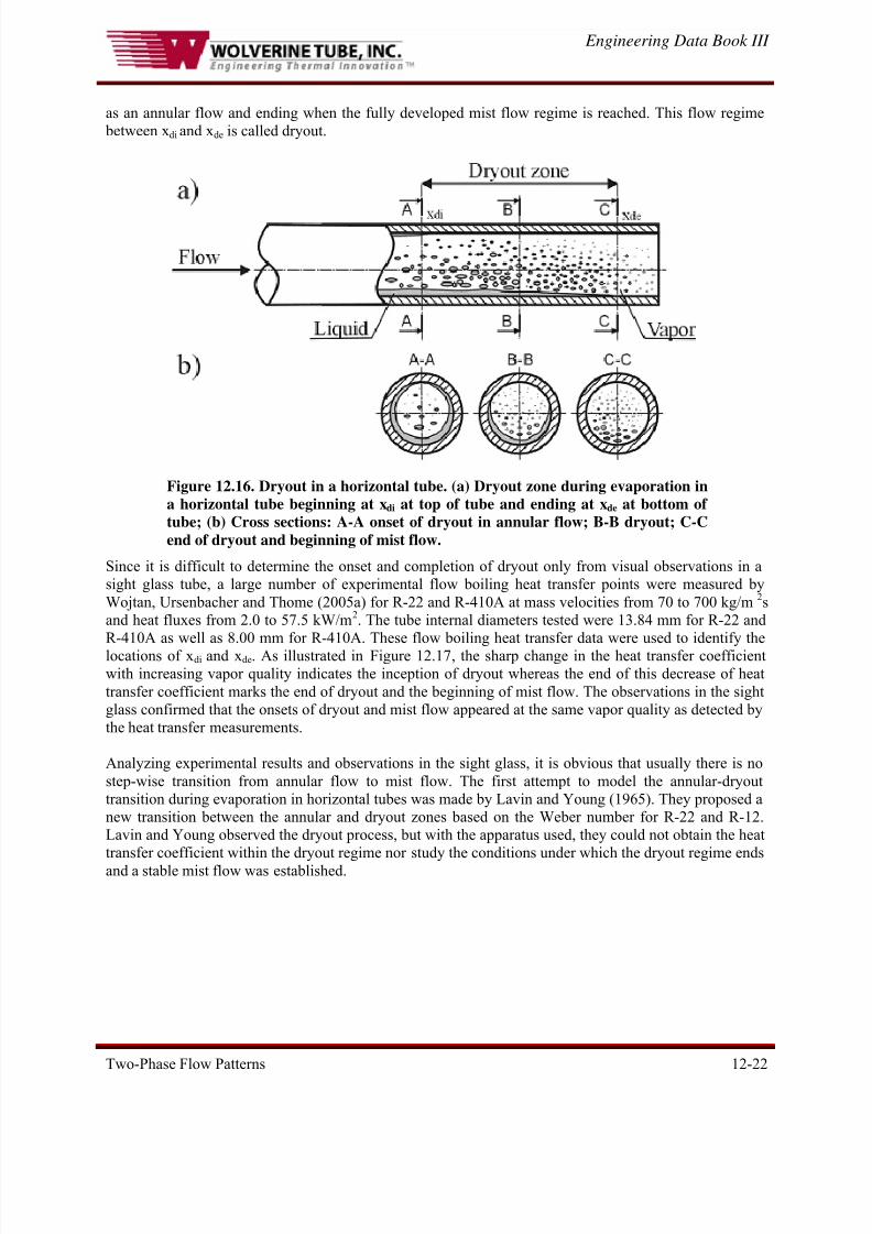
as an annular flow and ending when the fully developed mist flow regime is reached. This flow regime

between xdi and xde is called dryout.

Figure 12.16. Dryout in a horizontal tube. (a) Dryout zone during evaporation ina horizontal tube beginning at xdi at top of tube and ending at xde at bottom oftube; (b) Cross sections: A-A onset of dryout in annular flow; B-B dryout; C-C

end of dryout and beginning of mist flow.

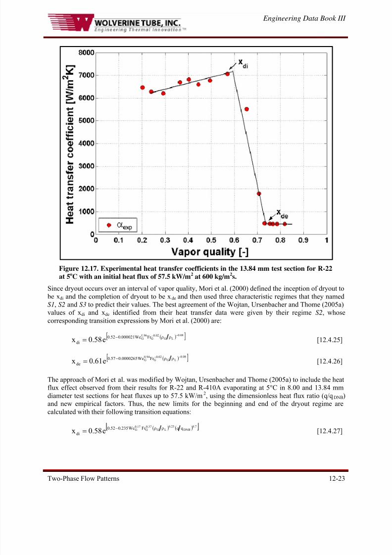
Since it is difficult to determine the onset and completion of dryout only from visual observations in a

sight glass tube, a large number of experimental flow boiling heat transfer points were measured by

Wojtan, Ursenbacher and Thome (2005a) for R-22 and R-410A at mass velocities from 70 to 700 kg/m 2s

and heat fluxes from 2.0 to 57.5 kW/m2. The tube internal diameters tested were 13.84 mm for R-22 and

R-410A as well as 8.00 mm for R-410A. These flow boiling heat transfer data were used to identify the

locations of xdi and xde. As illustrated in Figure 12.17, the sharp change in the heat transfer coefficient

with increasing vapor quality indicates the inception of dryout whereas the end of this decrease of heat

transfer coefficient marks the end of dryout and the beginning of mist flow. The observations in the sight

glass confirmed that the onsets of dryout and mist flow appeared at the same vapor quality as detected by

the heat transfer measurements.

Analyzing experimental results and observations in the sight glass, it is obvious that usually there is no

step-wise transition from annular flow to mist flow. The first attempt to model the annular-dryout

transition during evaporation in horizontal tubes was made by Lavin and Young (1965). They proposed a

new transition between the annular and dryout zones based on the Weber number for R-22 and R-12.

Lavin and Young observed the dryout process, but with the apparatus used, they could not obtain the heat

transfer coefficient within the dryout regime nor study the conditions under which the dryout regime ends

and a stable mist flow was established.





Figure 12.17. Experimental heat transfer coefficients in the 13.84 mm test section for R-22at 5oC with an initial heat flux of 57.5 kW/m2 at 600 kg/m2s.

Since dryout occurs over an interval of vapor quality, Mori et al. (2000) defined the inception of dryout to be xdi and the completion of dryout to be xde and then used three characteristic regimes that they named

S1, S2 and S3 to predict their values. The best agreement of the Wojtan, Ursenbacher and Thome (2005a)

values of xdi and xde identified from their heat transfer data were given by their regime S2, whose

corresponding transition expressions by Mori et al. (2000) are:

( )[ ]08.0LG

02.0G

96.0G Fr We000021.052.0

di e58.0x−− ρρ−= [12.4.25]

( )[ ]08.0LG

02.0G

94.0G Fr We0000265.057.0

de e61.0x−− ρρ−= [12.4.26]

The approach of Mori et al. was modified by Wojtan, Ursenbacher and Thome (2005a) to include the heat

flux effect observed from their results for R-22 and R-410A evaporating at 5°C in 8.00 and 13.84 mmdiameter test sections for heat fluxes up to 57.5 kW/m2, using the dimensionless heat flux ratio (q/qDNB)and new empirical factors. Thus, the new limits for the beginning and end of the dryout regime are

calculated with their following transition equations:

( ) ( ) 7.0DNB

25.0LG

37.0G

17.0G qqFr We235.052.0

di e58.0x ρρ−= [12.4.27]





( ) ( )[ ]27.0DNB

09.0LG

15.0G

38.0G qqFr We0058.057.0

de e61.0x−ρρ−= [12.4.28]

where qDNB is calculated with the expression [12.4.9] of Kutateladze (1948). After inversion of these two

equations to solve for the mass velocity in terms of vapor quality, the annular-to-dryout boundary (A-D)

and the dryout-to-mist flow boundary (D-M) transition equations for xdi and xde become respectively:

( )

926.07.0

DNB

25.0

L

G

37.0

VLGi

17.0

G

idryout

q

q

gd

1d52.0

x

58.0ln

235.0

1m

⎥⎥⎦

⎤

⎢⎢⎣

⎡⎟⎟ ⎠

⎞⎜⎜⎝

⎛ ⎟⎟ ⎠

⎞⎜⎜⎝

⎛

ρ

ρ⎟⎟ ⎠

⎞⎜⎜⎝

⎛

ρ−ρρ⎟⎟ ⎠

⎞⎜⎜⎝

⎛

σρ⎟⎟ ⎠

⎞⎜⎜⎝

⎛ +⎟

⎠

⎞⎜⎝

⎛ =−−−−

&

[12.4.29]

( )

943.027.0

DNB

09.0

L

G

15.0

VLGi

38.0

G

imist

q

q

gd

1d57.0

x

61.0ln

0058.0

1m

⎥⎥⎦

⎤

⎢⎢⎣

⎡⎟⎟ ⎠

⎞⎜⎜⎝

⎛ ⎟⎟ ⎠

⎞⎜⎜⎝

⎛

ρ

ρ⎟⎟ ⎠

⎞⎜⎜⎝

⎛

ρ−ρρ⎟⎟ ⎠

⎞⎜⎜⎝

⎛

σρ⎟⎟ ⎠

⎞⎜⎜⎝

⎛ +⎟

⎠

⎞⎜⎝

⎛ =−−−

&

[12.4.30]

Including the above modifications also to the stratified-wavy region and integrating the new A-D and D-

M transition curves into their map, the implementation procedure for the Wojtan-Ursenbacher-Thome

map is as follows:

1. The geometric parameters ε, ALd, AGd, hLd, Pid and θstrat are calculated using the expressions

[12.4.19] to [12.4.24], respectively.

2. As the effect of heat flux at high vapor quality is captured by the A-D and D-M transition curves,

the SW-I/A transition is first calculated from the following adiabatic version of expression

[12.4.1]:

( )[ ]501

Fr

We

h251h21x

gdA16m

5.01

L

L

2

Ld

2

5.02

Ld

22

GLi

3

Gdwavy +

⎪⎭

⎪⎬⎫

⎪⎩

⎪⎨⎧

⎥⎥⎦

⎤

⎢⎢⎣

⎡+⎟⎟

⎠

⎞⎜⎜⎝

⎛ π

−−π

ρρ=

−

& [12.4.31]

3. The stratified-wavy region is then subdivided into three zones as follows:

i. m& > m& wavy(xIA) gives the slug flow zone;

ii. m& strat < & < & wavy(xIA) and 0 < x < xIA give the Slug/Stratified-Wavy zone;

iii. 1 > x ≥ xIA gives the Stratified-Wavy zone.

4. The S-SW transition is calculated from the original boundary expression [12.4.4] but now & strat =

& strat(xIA) when x < xIA, the latter which gives the flat horizontal part of the boundary for 0 ≤ x ≤ xIA.

5. The I-A transition is calculated from the original boundary given by [12.4.11] and extended down

to its intersection with m& strat.

6. The A-D boundary is calculated from [12.4.29] where its value takes precedent over the value

from step 2 above when its value is smaller than m&wavy

.





7. The D-M boundary is calculated from [12.4.30] but since the A-D and D-M lines are not parallel

these boundaries can intersect, so that when xde < xdi then xde is set equal to the value of xdi and no

D region exists (at high mass velocities and low heat fluxes where this occurs, the high vapor

shear will tend to make the annular film to be of uniform thickness and hence it seems reasonable

that the entire perimeter becomes dry simultaneously at xdi).

8. The following logic is applied to define the transitions in the high vapor quality range for the

onset of dryout in the map, referred to as m& dryout, implemented in the following order:

• If m& strat(x) ≥ & dryout(x), then & dryout = m& strat(x);

• If & wavy(x) ≥ m& dryout(x), then m& dryout = & dryout(x) and the & wavy curve ceases to exist, which

means that the rightmost boundary of the m& wavy curve is its intersection with the & dryout curve;

• If m& dryout(x) ≥ & mist(x), which is possible at low heat fluxes and high mass velocities, then

m& dryout = m& dryout(x) and the dryout regime disappears at this mass velocity.

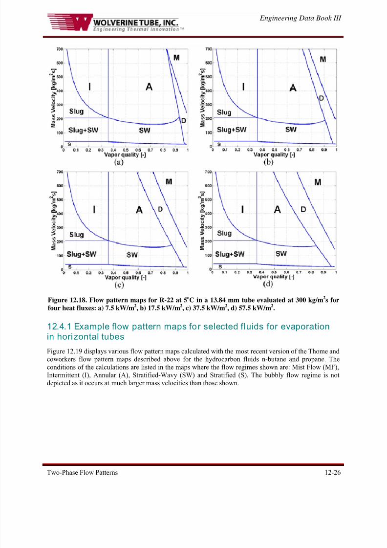
Figure 12.18 shows the flow pattern maps calculated for R-22 for four heat fluxes, where the movements

of the A-D and D-M boundaries are quite evident. Compared to the Kattan-Thome-Favrat map, the new

regimes slug (Slug), slug/stratified-wavy (Slug+SW) and dryout (D) are now encountered. Notably, it is

observed that the dryout and mist flow regions become smaller as the heat flux decreases.

This map was developed from a database for R-22 and R-410A at 5°C but its prior versions covered eight

other refrigerants (R-134a, R-123, R-402A, R-404A, R-502, R-407C, R-507A and ammonia) for tube

diameters from 8 to 14 mm. The test conditions in all these experiments covered the following range of

variables: mass flow rates from 16 to 700 kg/m2s, vapor qualities from 1-99% and heat fluxes from 440 to

57500 W/m2. It is believed that the map is appropriate for refrigerants (and fluids with similar physical properties such as light hydrocarbons) at low to medium pressures but not for CO2 (too high of operating

pressures for the map) nor for air-water or steam-water systems (their surface tension and density ratio are

too high with respect to the refrigerant database).





Figure 12.18. Flow pattern maps for R-22 at 5oC in a 13.84 mm tube evaluated at 300 kg/m2s forfour heat fluxes: a) 7.5 kW/m2, b) 17.5 kW/m2, c) 37.5 kW/m2, d) 57.5 kW/m2.

12.4.1 Example flow pattern maps for selected fluids for evaporationin horizontal tubes

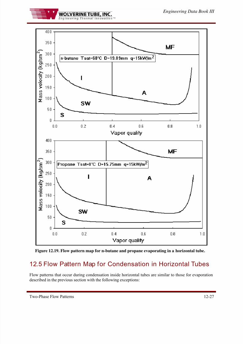
Figure 12.19 displays various flow pattern maps calculated with the most recent version of the Thome and

coworkers flow pattern maps described above for the hydrocarbon fluids n-butane and propane. The

conditions of the calculations are listed in the maps where the flow regimes shown are: Mist Flow (MF),

Intermittent (I), Annular (A), Stratified-Wavy (SW) and Stratified (S). The bubbly flow regime is not

depicted as it occurs at much larger mass velocities than those shown.





Figure 12.19. Flow pattern map for n-butane and propane evaporating in a horizontal tube.

12.5 Flow Pattern Map for Condensation in Horizontal Tubes

Flow patterns that occur during condensation inside horizontal tubes are similar to those for evaporation

described in the previous section with the following exceptions:





1. Dry saturated vapor is entering the tube and hence the process begins without any entrainment of

liquid while for evaporating flows the liquid bridging across the flow channel in churn and

intermittent flow can result in significant entrainment when these flow structures break up.

2. During evaporation, the annular film eventually dries out while for condensation no dryout occurs. In

fact, for condensation at high vapor qualities the flow is annular and there is no passage fromstratified-wavy flow into annular flow while for evaporation the flow reverts to stratified-wavy flow

at the onset of dryout at the top of the tube.

3. During condensation, the condensate formed coats the tube perimeter with a liquid film. In what

would otherwise be a mist flow for adiabatic or evaporating flows, in condensation the flow regime

will look like annular flow since the entrainment of liquid into the vapor core will leave bare surfaceavailable for rapid formation of a new liquid layer via condensation.

4. During condensation in stratified flow regimes, the top of the tube is wetted by the condensate film

while in adiabatic and evaporating flows the top perimeter is dry.

Hence, the three principal flow patterns encountered during condensation inside horizontal tubes are:

• Annular flow (often referred to as the shear-controlled regime in condensation heat transfer

literature);

• Stratified-wavy flow (characterized by waves on the interface of the stratified liquid flowing along

the bottom of the tube with film condensation on the top perimeter);

• Stratified flow (no interfacial waves on the stratified liquid flowing along the bottom of the tube with

film condensation on the top perimeter that drains into the stratified liquid).

The latter are sometimes referred to as the gravity-controlled regime in condensation heat transfer

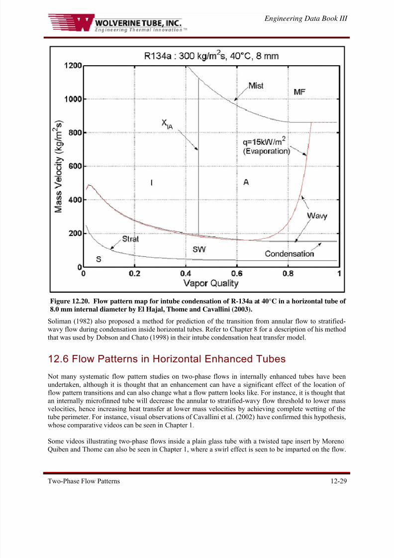
literature. These flow regimes can tentatively be predicted using the Kattan-Thome-Favrat flow pattern

maps for intube evaporation as proposed by El Hajal, Thome and Cavallini (2003). First, the mist flow

transition is eliminated because flow in this zone may be considered to be annular flow since a condensatefilm is always formed, even if the liquid is then entrained. Secondly, the stratified-wavy transition curve

is modified by first eliminating the transition from annular flow to stratified-wavy flow at high vapor

qualities by solving for the minimum in the stratified-wavy flow transition curve and then extending this

curve as a straight line from that point to the end of the stratified transition curve for at a vapor

quality of x = 1.0.

stratm&

Figure 12.20 illustrates this flow pattern map for condensation of R-134a at 40°C in a

horizontal tube of 8.0 mm internal diameter.





Figure 12.20. Flow pattern map for intube condensation of R-134a at 40°C in a horizontal tube of8.0 mm internal diameter by El Hajal, Thome and Cavallini (2003).

Soliman (1982) also proposed a method for prediction of the transition from annular flow to stratified-

wavy flow during condensation inside horizontal tubes. Refer to Chapter 8 for a description of his method

that was used by Dobson and Chato (1998) in their intube condensation heat transfer model.

12.6 Flow Patterns in Horizontal Enhanced Tubes

Not many systematic flow pattern studies on two-phase flows in internally enhanced tubes have been

undertaken, although it is thought that an enhancement can have a significant effect of the location of

flow pattern transitions and can also change what a flow pattern looks like. For instance, it is thought thatan internally microfinned tube will decrease the annular to stratified-wavy flow threshold to lower mass

velocities, hence increasing heat transfer at lower mass velocities by achieving complete wetting of the

tube perimeter. For instance, visual observations of Cavallini et al. (2002) have confirmed this hypothesis,

whose comparative videos can be seen in Chapter 1.

Some videos illustrating two-phase flows inside a plain glass tube with a twisted tape insert by Moreno

Quiben and Thome can also be seen in Chapter 1, where a swirl effect is seen to be imparted on the flow.





Again, it is believed that the annular-stratified wavy transition threshold m& wavy is displaced to lower mass

velocities, but this was not systematically documented, however.

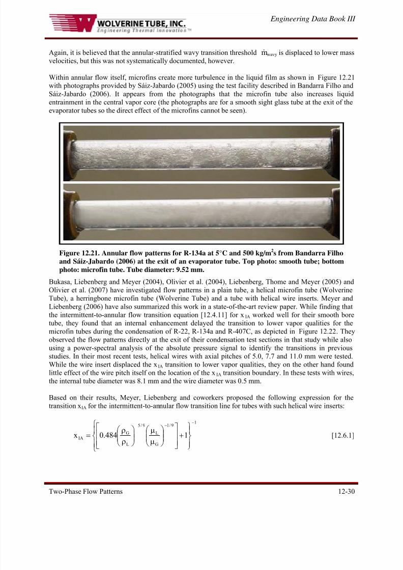
Within annular flow itself, microfins create more turbulence in the liquid film as shown in Figure 12.21 with photographs provided by Sáiz-Jabardo (2005) using the test facility described in Bandarra Filho and

Sáiz-Jabardo (2006). It appears from the photographs that the microfin tube also increases liquid

entrainment in the central vapor core (the photographs are for a smooth sight glass tube at the exit of theevaporator tubes so the direct effect of the microfins cannot be seen).

Figure 12.21. Annular flow patterns for R-134a at 5°C and 500 kg/m2s from Bandarra Filhoand Sáiz-Jabardo (2006) at the exit of an evaporator tube. Top photo: smooth tube; bottom

photo: microfin tube. Tube diameter: 9.52 mm.

Bukasa, Liebenberg and Meyer (2004), Olivier et al. (2004), Liebenberg, Thome and Meyer (2005) and

Olivier et al. (2007) have investigated flow patterns in a plain tube, a helical microfin tube (Wolverine

Tube), a herringbone microfin tube (Wolverine Tube) and a tube with helical wire inserts. Meyer andLiebenberg (2006) have also summarized this work in a state-of-the-art review paper. While finding that

the intermittent-to-annular flow transition equation [12.4.11] for xIA worked well for their smooth bore

tube, they found that an internal enhancement delayed the transition to lower vapor qualities for the

microfin tubes during the condensation of R-22, R-134a and R-407C, as depicted in Figure 12.22. They

observed the flow patterns directly at the exit of their condensation test sections in that study while also

using a power-spectral analysis of the absolute pressure signal to identify the transitions in previous

studies. In their most recent tests, helical wires with axial pitches of 5.0, 7.7 and 11.0 mm were tested.

While the wire insert displaced the xIA transition to lower vapor qualities, they on the other hand found

little effect of the wire pitch itself on the location of the xIA transition boundary. In these tests with wires,

the internal tube diameter was 8.1 mm and the wire diameter was 0.5 mm.

Based on their results, Meyer, Liebenberg and coworkers proposed the following expression for thetransition xIA for the intermittent-to-annular flow transition line for tubes with such helical wire inserts:

⎪⎩

⎪⎨

⎧

⎪⎭

⎪⎬⎫

+⎥⎥⎦

⎤

⎢⎢⎣

⎡⎟⎟ ⎠

⎞⎜⎜⎝

⎛

μμ

⎟⎟ ⎠

⎞⎜⎜⎝

⎛

ρρ

=

−−−

19/1

G

L

9/5

L

GIA 1484.0x

[12.6.1]





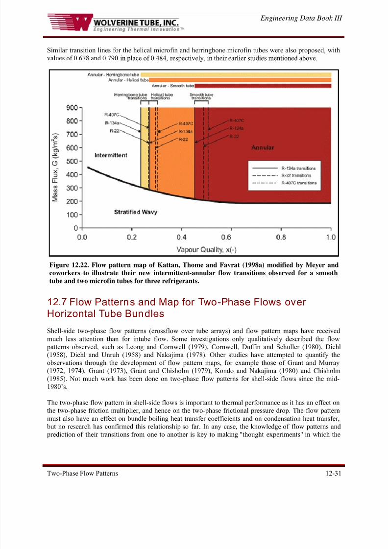
Similar transition lines for the helical microfin and herringbone microfin tubes were also proposed, with

values of 0.678 and 0.790 in place of 0.484, respectively, in their earlier studies mentioned above.

Figure 12.22. Flow pattern map of Kattan, Thome and Favrat (1998a) modified by Meyer andcoworkers to illustrate their new intermittent-annular flow transitions observed for a smooth

tube and two microfin tubes for three refrigerants.

12.7 Flow Patterns and Map for Two-Phase Flows overHorizontal Tube Bundles

Shell-side two-phase flow patterns (crossflow over tube arrays) and flow pattern maps have received

much less attention than for intube flow. Some investigations only qualitatively described the flow

patterns observed, such as Leong and Cornwell (1979), Cornwell, Duffin and Schuller (1980), Diehl

(1958), Diehl and Unruh (1958) and Nakajima (1978). Other studies have attempted to quantify the

observations through the development of flow pattern maps, for example those of Grant and Murray

(1972, 1974), Grant (1973), Grant and Chisholm (1979), Kondo and Nakajima (1980) and Chisholm

(1985). Not much work has been done on two-phase flow patterns for shell-side flows since the mid-

1980’s.

The two-phase flow pattern in shell-side flows is important to thermal performance as it has an effect on

the two-phase friction multiplier, and hence on the two-phase frictional pressure drop. The flow pattern

must also have an effect on bundle boiling heat transfer coefficients and on condensation heat transfer,

but no research has confirmed this relationship so far. In any case, the knowledge of flow patterns and

prediction of their transitions from one to another is key to making "thought experiments" in which the





two-phase flow structure in new systems can be predicted. Such predictions are helpful in establishing

what the operating characteristics of the system will be, and thus avoid potential operating problems.

Leong and Cornwell (1979) and Cornwell, Duffin and Schuller (1980) have made visual observations of

two-phase flows in a kettle reboiler slice during evaporation. They reported that two main flow patterns

are dominant. In the lower zone of their 241-tube inline tube bundle, the flow was predominantly bubbly.

In the upper zone where the vapor quality is larger, a distinct change in the appearance of the flowoccurred, where it took on a "frothy" character. This transition was estimated to occur at a void fraction of

about 60%. On the other hand, for a staggered tube bundle with two-phase upflow, Nakajima (1978)

observed only bubbly and slug flows for tests at very low mass velocities and low qualities. For

downflow at much higher mass velocities for a staggered tube bundle, Diehl (1957) observed only annular

and spray flows. Diehl and Unruh (1958) described spray flow as one with a high-entrained liquid

fraction while they defined annular flow as a flow with a low entrainment. In a more comprehensive

study, Grant and Chisholm (1979) studied vertical upflow and downflow over a wide range of mass

velocities and qualities in a staggered tube array, observing bubbly, intermittent (slug), and spray flows.

The Diehl and Diehl-Unruh annular flow observations are probably the same as the spray flow category

of Grant and Chisholm.

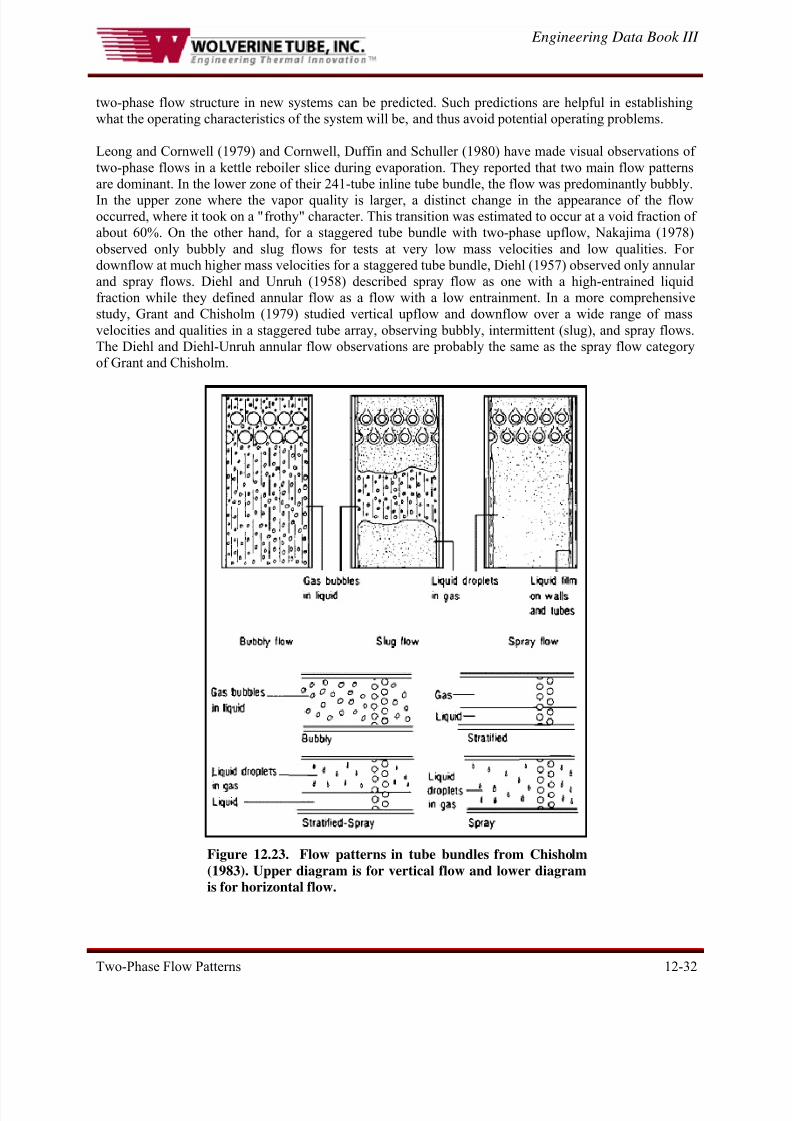
Figure 12.23. Flow patterns in tube bundles from Chisholm

(1983). Upper diagram is for vertical flow and lower diagramis for horizontal flow.





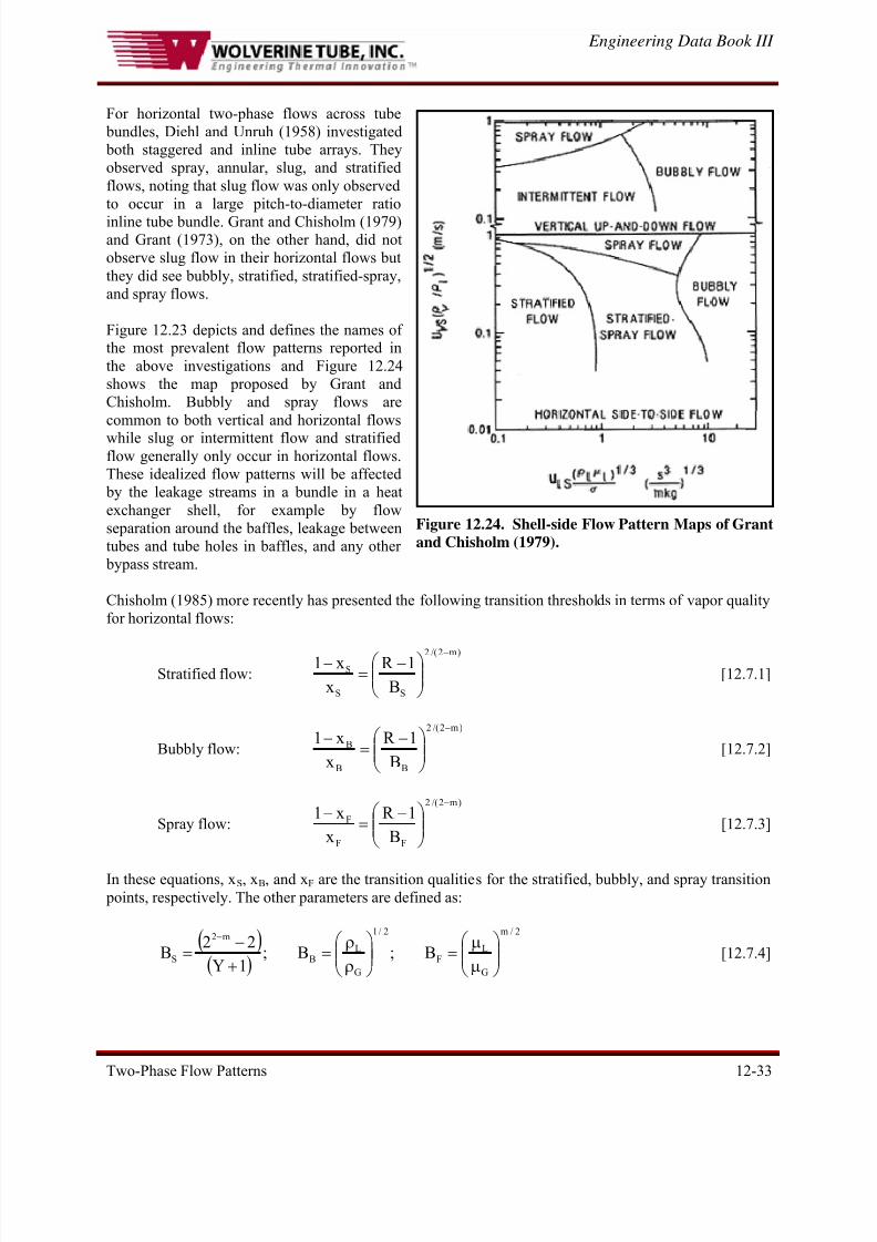
For horizontal two-phase flows across tube

bundles, Diehl and Unruh (1958) investigated

both staggered and inline tube arrays. They

observed spray, annular, slug, and stratified

flows, noting that slug flow was only observed

to occur in a large pitch-to-diameter ratio

inline tube bundle. Grant and Chisholm (1979)and Grant (1973), on the other hand, did not

observe slug flow in their horizontal flows but

they did see bubbly, stratified, stratified-spray,

and spray flows.

Figure 12.24. Shell-side Flow Pattern Maps of Grantand Chisholm (1979).

Figure 12.23 depicts and defines the names ofthe most prevalent flow patterns reported in

the above investigations and Figure 12.24

shows the map proposed by Grant and

Chisholm. Bubbly and spray flows are

common to both vertical and horizontal flows

while slug or intermittent flow and stratifiedflow generally only occur in horizontal flows.

These idealized flow patterns will be affected

by the leakage streams in a bundle in a heat

exchanger shell, for example by flow

separation around the baffles, leakage between

tubes and tube holes in baffles, and any other

ypass stream.

e recently has presented the following transition thresholds in terms of vapor quality

r horizontal flows:

Stratified flow:

b

Chisholm (1985) mor

fo

)m2/(2

SS

S

B

1R

x

x1 −

⎟⎟ ⎠

⎞⎜⎜⎝

⎛ −=

− [12.7.1]

Bubbly flow:

)m2/(2

BB

B

B

1R

x

x1−

⎟⎟ ⎠

⎞⎜⎜⎝

⎛ −=

− [12.7.2]

Spray flow:

)m2/(2

FF

F

B

1R

x

x1−

⎟⎟ ⎠

⎞⎜⎜⎝

⎛ −=

− [12.7.3]

In these equations, xS, xB, and xB

s for the stratified, bubbly, and spray transition

oints, respectively. The other parameters are defined as:F are the transition qualitie

p

( )( )

2/m

G

LF

2/1

G

LB

m2

S B;B;1Y

22B ⎟⎟

⎠

⎞⎜⎜⎝

⎛

μμ

=⎟⎟ ⎠

⎞⎜⎜⎝

⎛

ρρ

=+−

=−

[12.7.4]




m

G

L2

L NFr 59.03.1R ⎟⎟ ⎠

⎞⎜⎜⎝

⎛

μμ

+= [12.7.5]

m

G

L

G

L

LG dz

dp/

dz

dpY

−

⎟⎟ ⎠

⎞

⎜⎜⎝

⎛

μ

μ

⎟⎟ ⎠

⎞

⎜⎜⎝

⎛

ρ

ρ=

⎟ ⎠

⎞

⎜⎝

⎛

⎟ ⎠

⎞

⎜⎝

⎛ = [12.7.6]

and m is the exponent in a Blasius-type single-phase friction factor equation. The quantity Fr L, is the

Froude number for the total flow as liquid with the velocity based on the minimum cross-sectional area in

the tube bundle normal to the flow direction. The reliability of general use of these methods for prediction

of flow pattern transitions is not able to be qualified here.

CONCLUSIONS

Flow patterns have an important influence on prediction of the void fraction, flow boiling and convective

condensation heat transfer coefficients, and two-phase pressure drops. The prediction of flow pattern

transitions and their integration into a flow pattern map for general use is thus of particular importance tothe understanding of two-phase flow phenomena and design of two-phase equipment.

For vertical tubes, the flow pattern maps of Fair (1960) and Hewitt and Roberts (1969) are those most

widely recommended for use. For horizontal tubes, the methods of Taitel and Dukler (1976) and Baker

(1954) are widely used. The more recent flow pattern map of Kattan, Thome and Favrat (1998a) and itsmore subsequent improvements, which was developed specifically for small diameter tubes typical of

shell-and-tube heat exchangers for both adiabatic and evaporating flows, is that recommended here for

heat exchanger design. Another version of their map has also been proposed by El Hajal, Thome and

Cavallini (2003) for intube condensation.

Shell side flow patterns and flow patterns maps have received very little attention compared to intube

studies. Qualitative and quantitative attempts have been made to obtain flow pattern maps, but to date nomethod has been shown to be of general application. The flow pattern map of Grant and Chisholm (1979)

has been presented here but its use must be taken as a best estimate only at this point.

-------------------------------------------------------------------------------------------------------------------------------

Example Calculation: A two-phase fluid is flowing upwards in a vertical pipe of internal diameter of 1.0

in. The fluid properties are as follows: liquid density = 60 lb/ft3; vapor density = 2 lb/ft3; liquid viscosity =

0.4 cp; vapor viscosity = 0.01 cp. If the vapor quality is 0.2 and the total flow rate of liquid and vapor is

3600 lb/h, using the Fair flow pattern map, what is the local flow pattern expected to be?

Solution: The mass flow rate of 3600 lb/h is equivalent to 1.0 lb/s. The internal diameter is 1 in. = 1/12 ft.

The mass velocity is then obtained by dividing the mass flow rate by the internal cross-sectional area of

the tube, such that the mass velocity = 183.3 lb/s ft2. The parameter on the x-axis of the Fair map is:

09.14.0

01.0

2

60

2.01

2.0

x1

x1.05.09.01.0

L

G

5.0

G

L

9.0

=⎟ ⎠

⎞⎜⎝

⎛ ⎟ ⎠

⎞⎜⎝

⎛ ⎟ ⎠

⎞⎜⎝

⎛ −

=⎟⎟ ⎠

⎞⎜⎜⎝

⎛

μμ

⎟⎟ ⎠

⎞⎜⎜⎝

⎛

ρρ

⎟ ⎠

⎞⎜⎝

⎛ −

Thus, using the values of 183.3 and 1.09 on the map, the flow regime is identified to be annular flow.

Documents

Flow Pattern in Horizontal and Vertical Tubes