TECHNICAL NOTE

1 ISS TECHNICAL NOTE

FLIM Analysis using the Phasor Plots Shih-Chu Liao, Yuansheng Sun, Ulas Coskun ISS, Inc.

1 Introduction

Given a number 0N of molecules in the excited state at time 0t , the fluorescence decay time is the time it takes

for the population to decrease by 1e, or about 36.8% of the initial value. The process is accomplished with the

emission photons, or fluorescence. The natural fluorescence lifetime of a fluorophore in the absence of non-radiative

processes is an intrinsic property of the fluorophore. The fluorescence lifetime of a fluorescent molecule carries

information about its local microenvironment and can be very sensitive to certain environmental changes. Therefore,

cellular responses to events such as changes in temperature, pH, and ion concentrations (e.g. Calcium) can be

measured accurately using Fluorescence Lifetime Imaging Microscopy (FLIM). FLIM is now routinely used for

dynamic measurements of signaling events inside living cells, including detection of protein-protein interactions (1).

The traditional approach for the fluorescence time determination consists in using the least-square fitting analysis at

each pixel or each group of binned pixels in the image. This approach requires indeed some level of expertise in the

choice of the fitting model and a full appreciation of the statistical tools that are to be utilized in cases that are at best

disputable. The process can be time consuming for a large amount of data since it typically runs on a pixel-by-pixel

basis. Also, the process can easily bring to inaccuracies in the determination of decay times when several decay

processes are present, as it is commonly the case for cell biology. In comparison, the phasor plot analysis approach

streamlines the procedure and allows for the quantitative determination of fluorescence lifetimes and even Förster

resonance energy transfer (FRET) efficiencies. Please see our application note “The ultimate phasor plot and

beyond” for a list of merits of the phasor plot with examples.

2 The non-linear least square fitting

In fluorescence lifetime imaging, the decay times of fluorophores are determined at each spatial location of an image.

Assuming an infinite short excitation pulse (δ-function), an intrinsic fluoresce decay composed of N (N≥1) fluorescent

species with distinct fluoresce lifetimes can be modeled by Eq. [1].

1

( ) (0) i

tN

iiI t I e

[ 1]

Where (0)I

is the number of the instantly emitted photons at time zero; the coefficient i , called the pre-

exponential factor, is the amplitude and i is the fluorescence decay time of the i-th component of the mixture. The

2 ISS TECHNICAL NOTE

amplitude weighted lifetime a (often called apparent lifetime) given by Eq. [2] is typically used for the calculation of

the energy transfer efficiency. The average lifetime is given by Eq. [3], where if is the fractional contribution of

the i-th species to the total intensity

N

i iia 1 [ 2]

N

i iif1 aiif [ 3]

Due to the finite response of a system, the measured decay signal ( )I t is a convolution form of the intrinsic decay

and the instrument response function (IRF) plus the noise ( )n t , as shown in Eq. [4].

tneIIRFtntIIRFtIN

i

t

ii

1)0(ˆ)(ˆ)(

[ 4]

Thus, accurate FLIM data analysis typically requires the calibration of the IRF. In time-domain FLIM, the IRF can be

measured by recording the scattered excitation light when using one-photon excitation, or the second-harmonic

generation (SHG) signals for two-photon excitation by using a sample that yields strong SHG, such as urea crystal.

In frequency-domain FLIM, the IRF is typically calibrated with a fluorescence lifetime standard of known lifetime. A

list of these standards is given on the ISS website.

http://www.iss.com/resources/reference/data_tables/FL_LifetimeStandards.html

http://www.iss.com/resources/reference/data_tables/LifetimeDataFluorophores.html

Most FLIM data analysis routines involve fitting of the measured data based on a specified decay kinetics model (Eq.

[1]). An iteratively constrained optimization algorithm is typically applied to estimate the fitting parameters, i.e.

lifetime(s) and pre-exponential factor(s) – at each iteration step, the result calculated from the estimated parameters

based on the decay model is compared to the measured data, providing a feedback for updating the fitting

parameters as well as a criterion for terminating the iterative optimization process. Through the years several

optimization approaches have been used, and a partial list includes: the non-linear least square analysis, the method

of moments, maximum entropy, the Laplace transform, the phase plane, the Prony’s method, the sine transform,

maximum likelihood expectation minimization. For statistical robustness, the method of choice is today the non-linear

least square analysis in both time- and frequency-domain analysis.

An important criterion to assess the goodness of the fit for the non-linear least square analysis is the calculated chi-

square. In the VistaVision software by ISS, the chi-square functions for both time-correlated single-photon counting

(TCSPC) and frequency-domain (FD) FLIM data fitting are minimized using the Levenberg-Marquardt algorithm, as

shown below.

3 ISS TECHNICAL NOTE

2.1 Definition of Chi-Square 2 for TCSPC FLIM data

The observable to be measured in TCSPC FLIM is the number of photons in each acquisition bin (N).

The reduced 2 function is defined by Eq. [5]:

n

k k

kckn

k k

kck

tN

tNtN

pn

tNtN

pn 1

2

12

2

2

1

1

1

1

[ 5]

Where n is the number of acquisition bins; p is the number of the fitting parameters; N(tk) is the number of photons

collected and Nc(tk) is the number of photons calculated from the estimated fitting parameters based on the chosen

decay model, in each data acquisition bin k; k is the standard deviation, and for a large number of photon counts

following the Poisson distribution it is equal to the square root of N(tk).

2.2 Definition of Chi-Square 2 for FD FLIM data

The observables to be measured in FD FLIM are, for each modulation frequency , the phase delay (φ) and the

amplitude modulation ratio (m). The reduced 2 function is defined by Eq. [6]:

n

k

n

k mk

ckk

k

ckk mm

pn 1 1

22

2

12

1

[ 6]

Where n is the number of modulation frequencies; p is the number of the fitting parameters; φk and mk are the

measured phase shift and modulation ratio, while φck and mck are the calculated phase shift and modulation ratio

using the estimated fitting parameters based on the selected decay model, at frequency k; φk and mk are the

uncertainties in the phase and modulation ratio values, respectively. It should be noted that the digital FD (DFD)

FLIM approach implemented in ISS FastFLIM carries out multi-modulation-frequency measurements simultaneously,

allowing much faster data acquisition than the traditional FD FLIM methods, which measure at multiple frequencies in

a sequential way.

2.3 Challenges in the non-linear least square fitting for FLIM data analysis

Using the non-linear least-square fitting for FLIM data analysis, the approach utilized by the user typically

encompasses the following sequential steps:

Establish a decay model such as the N value in Eq. [1]; In most cases, one first starts from the simplest model,

i.e. the single exponential decay;

Make initial guesses to the physical parameters such as αi and τi in Eq. [1] and specify their constraints such as

the range of each value upon known priori information.

4 ISS TECHNICAL NOTE

Click the “fit” button in the software to let the computer algorithm estimate the results.

Examine the fit by checking the chi-square value and the fitting residuals.

If the fit is not acceptable, go back to the first step to apply a more complicated decay model, typically by adding

one more exponent, and start over...

It is often straightforward to apply the above steps in commercial software, e.g. VistaVision by ISS. Assessing the fit

of the FLIM data, however, can still be challenging. Even though the chi-square value provides a quantitative

measurement for fitting, there is no golden rule made only based on it to accept or reject a fitting model. This is

simply because the photon counts in most of real experiments are limited and far less than the statistical requirement.

Therefore, the traditional non-linear fitting for FLIM data analysis indeed requires some level of expertise in

understanding the physics of fluorescence lifetime and a full appreciation of the statistical tools that are to be utilized

in cases that are at best disputable.

3 The phasor plot

The phasor plot, also known as the AB plot or the polar plot (2-6), is a graphic representation of the raw FLIM data.

Transforming FD or TCSPC FLIM data into the phasor plot is described below.

3.1 The phasor plot for FD FLIM data

For one modulation frequency (ω), the FD FLIM data measurements at each pixel location are composed of both the

phase delay (φ) and the amplitude modulation ratio (m) (see Figure 1). The FD FLIM data at each pixel can be

mapped to a single point called “phasor” in the phasor plot through a transform defined by Eq. [7], where g and s

represent the values at the two coordinates (G, S) of the phasor plot.

cosmg and sinms [ 7]

3.2 The phasor plot for TCSPC FLIM data

In TCSPC FLIM, a decay trace I(t) (see Eq. [4]) is recorded at each pixel location; each decay trace can be plotted as

a single point (“phasor”) in the phasor plot by applyin g the sine and cosine transforms to the measured decay data,

as shown by Eq. [8] and Figure 1. This is equivalent to the real and imaginary components of the Fourier transform of

the decay data.

tI

ttIg

0

0cos

and

tI

ttIs

0

0sin

[ 8]

Where the modulation frequency ω is now called the laser repetition angular frequency and calculated by multiplying

the laser repetition rate with 2π.

5 ISS TECHNICAL NOTE

Figure 1: Mapping FD and TCSPC FLIM data to the phasor plot.

3.3 Calibrating the phasor plot

In order to establish the correct scale for the plotted phasor points, the coordinates of the phasor plot need to be

calibrated using a standard sample of known lifetime. This is indeed the calibration of the IRF.

In FD FLIM, this is already done when calibrating the instrument prior to the data acquisition.

In TCSPC FLIM, this can be done by applying the Fourier transform to a recorded decay trace of known lifetime,

e.g. a decay acquired using Fluorescein at pH 9 (4 ns lifetime); alternatively, a directly recorded IRF data trace

for the zero lifetime can be used for the Fourier transform.

3.4 Phasor vs. lifetime

By taking Eq. [1] into Eq. [8] and solving the integrals, we can then derive the following relationships between the

phasor and the lifetime, given by Eq. [9].

N

i i

ifg1

221 and

N

i i

iifs1

221

[ 9]

As explained above in Eq. [1-3], N is the number of the fluorescent species, and fi is the fractional contribution of the i-

th species of the fluorescence lifetime τi to the total intensity.

6 ISS TECHNICAL NOTE

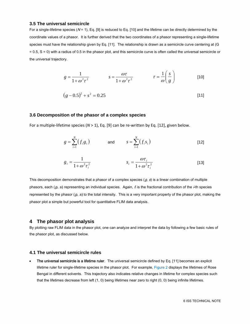
3.5 The universal semicircle

For a single-lifetime species (N = 1), Eq. [9] is reduced to Eq. [10] and the lifetime can be directly determined by the

coordinate values of a phasor. It is further derived that the two coordinates of a phasor representing a single-lifetime

species must have the relationship given by Eq. [11]. The relationship is drawn as a semicircle curve centering at (G

= 0.5, S = 0) with a radius of 0.5 in the phasor plot, and this semicircle curve is often called the universal semicircle or

the universal trajectory.

221

1

g

221

s

g

s

1 [10]

25.05.0 22 sg [11]

3.6 Decomposition of the phasor of a complex species

For a multiple-lifetime species (N > 1), Eq. [9] can be re-written by Eq. [12], given below.

N

i

ii gfg1

and

N

i

ii sfs1

[12]

221

1

i

ig

221 i

i

is

[13]

This decomposition demonstrates that a phasor of a complex species (g, s) is a linear combination of multiple

phasors, each (gi, si) representing an individual species. Again, fi is the fractional contribution of the i-th species

represented by the phasor (gi, si) to the total intensity. This is a very important property of the phasor plot, making the

phasor plot a simple but powerful tool for quantitative FLIM data analysis.

4 The phasor plot analysis

By plotting raw FLIM data in the phasor plot, one can analyze and interpret the data by following a few basic rules of

the phasor plot, as discussed below.

4.1 The universal semicircle rules

The universal semicircle is a lifetime ruler. The universal semicircle defined by Eq. [11] becomes an explicit

lifetime ruler for single-lifetime species in the phasor plot. For example, Figure 2 displays the lifetimes of Rose

Bengal in different solvents. This trajectory also indicates relative changes in lifetime for complex species such

that the lifetimes decrease from left (1, 0) being lifetimes near zero to right (0, 0) being infinite lifetimes.

7 ISS TECHNICAL NOTE

The scale of the semicircle ruler is adjustable upon the modulation frequency. Given the same single-lifetime

value, the phasor shifts to the left along the semicircle for a lower modulation frequency “ω” which results in an

increase of the “s/g” ratio (see Eq. [10]). An example comparing the phasor plots of two modulation frequencies

is shown in Figure 3. Thus, the scale of the semicircle ruler can be easily adjusted by changing the modulation

frequency to draw the phasor plot, making the phasor plot very flexible to visualize different lifetimes and

highlight the contrast upon the lifetime values. Typically, the available modulation frequencies are the integer

multiples of the fundamental modulation frequency. The measurements of different modulation frequencies are

performed simultaneously by ISS FastFLIM, and choosing a proper modulation frequency to make the phasor

plot is as easy as a simple click in the ISS VistaVision software.

Single-lifetime species are on the semicircle. As defined by Eq. [10-11], a phasor point or population falling or

centering at a point on the semicircle indicates a single-lifetime specie.

Complex species are inside the semicircle. As defined by Eq. [12], the phasor of a complex species is a linear

combination of the individual phasors of single-lifetime species. Connecting these individual phasors on the

semicircle yields a convex set inside the semicircle, and thus a species of multiple lifetime components must fall

inside the semicircle.

Excited-state products are outside the semicircle. In most FLIM measurements, every fluorescent component

contributing the measured lifetime is excited directly by the excitation light and the corresponding phasor should

never be outside the semicircle, assuming no perturbation from noise. However, when a fluorescent component

is an excited-state product, e.g. the sensitized emission of the acceptor produced by the energy transfer from the

excited-state donor in a FRET event, its phasor would locate outside the semicircle.

Figure 2: Decay time of Rose Bengal in different solvents displayed in the

phasor plot. Data was acquired using the ISS Alba V system using the 561 nm laser excitation. (Courtesy of Dr. Ammasi Periasamy, University of Virginia)

8 ISS TECHNICAL NOTE

Figure 3: Comparison of the phasor plot scales of two different modulation

frequencies.

4.2 The phasor decomposition rules

Decomposing the phasor of a complex species is a linear process, described by Eq. [12]. As shown in

Figure 4, the phasor point of a mixture composed of two species must lie on the line connecting the two

phasors of representing each individual species, and the contribution from one species to the mixture is

proportional to the distance from the mixture point to the other species point; for more components, the

mixture must locate inside the convex set connecting all the phasors of individual species (e.g. a triangle for

3 components). An example of comparing the mixture of two species vs. the two individual species is shown

in Figure 5.

The phasor decomposition is often not to solve the individual single-lifetime components. It should be noted

that the decomposed individual species does not have to be a single-lifetime species, e.g. the A-B mixture

case shown in Figure 4, where both species A and B have multiple lifetime components. This is a key

concept of using the phasor plot to analyze a complex system, where it is almost impossible to solve

individual lifetime components

9 ISS TECHNICAL NOTE

Figure 4: The phasor linear decomposition.

Figure 5: Comparison of mCerulean, mTurquise2 and three mixtures of the two

species in the phasor plot. Data was acquired using the ISS Alba V system using the 440 nm laser excitation source. (Courtesy of Dr. Richard N. Day; Indiana University School of Medicine)

4.3 The FRET trajectory approach for quantitative FRET data analysis

FRET is non-radiative energy transfer from an excited molecule (the donor) to another nearby molecule (the

acceptor) through a long range dipole–dipole coupling mechanism. As given by Eq. [13], the efficiency of energy

transfer (E) from the donor to the acceptor is dependent on the inverse of the sixth power of the distance separating

them (r), subject to their Förster distance (Ro) at which E is 50% (7-8). FRET is typically limited to distances less

than about 10 nm, making it a powerful tool for investigating a variety of phenomena that produce changes in

molecular proximity.

10 ISS TECHNICAL NOTE

66

6

oo

o

rR

RE

and

6/11

E

ERr o

[14]

FLIM is among the most accurate methods of measuring FRET (1). In a FLIM-FRET experiment, the quenched

lifetimes of the donor (τDA) in the samples containing both the donor and the acceptor are measured to map the FRET

efficiencies based on Eq. [14], where the unquenched donor lifetime (τD) is typically determined from the donor-only

control sample. As only donor signals are measured by FLIM for determining the FRET efficiency, the method does

not require the corrections for spectral bleedthrough that are necessary for intensity-based measurements of

sensitized emission from the acceptor.

D

DAE

1 [15]

In the phasor plot, it is easy to visualize the difference of the lifetimes from unquenched vs. quenched donor samples;

however, it does not seem to be straightforward to link both the data of both unquenched and quenched donors to

produce the FRET efficiency. Fortunately, Dr. Gratton’s LFD group came up an elegant solution, called the FRET

trajectory approach (2). The basic principle of this approach is illustrated in Figure 6, and is to decompose the

quenched donor phasor measured from the donor in the presence of the acceptor into three species:

The unquenched donor species with the lifetime of (τD) – the phasor of this species can be measured

independently from the donor-only control sample.

The background species with an arbitrary lifetime – the phasor of this species can be determined independently

from the unlabeled control sample.

The quenched donor species with the lifetime of (τDA) – its phasor can be calculated for any FRET efficiency

value ranging from 0 to 1, given the unquenched donor (τD) to Eq. [14].

Given the fraction contribution of each species, the phasor composed of the three species (unquenched donor, the

background and the quenched donor) for any FRET efficiency value can be located on the phasor plot – connecting

all phasor points corresponding to FRET efficiencies ranging from 0 to 1 makes a trajectory, named FRET trajectory.

Each point on the trajectory represents a FRET efficiency value. Both the starting (E = 0) and the ending (E ≈ 1)

points of a FRET trajectory are on the line of connecting the unquenched donor and the background phasors, while

the starting and the ending positions depend on the fraction contributions of the background and the unquenched

donor (see Figure 6):

When the fraction contribution from the background (fB) is zero, a FRET trajectory would always start from the

unquenched donor phasor point.

When the fraction contribution from the unquenched donor (fD) is zero, a FRET trajectory would always ends at

the background phasor point.

Likely, both background and unquenched donor give some fraction contributions – in this case, more fraction

contribution given by the background will push the starting point further way from the unquenched donor phasor,

and more fraction contribution from the unquenched donor will shift the ending point further way from the

background phasor.

11 ISS TECHNICAL NOTE

The goal now comes to find the FRET trajectory to pass through the measured quenched donor phasor and then

simply read its FRET efficiency at the intersection. The ISS VistaVision software makes this a step-by-step routine

requiring no expertise, as outlined below:

Load unquenched (donor-only), background (unlabeled) and quenched (donor + acceptor) data (images) into the

phasor plot using the “Multi-Image Phasor Analysis” module (see Figure 7). In this example, the background

data is ignored by assuming the zero lifetime for it.

Select the population of the unquenched donor (Cerulean-alone in this example) phasor points using the circle

shown on the phasor plot and assign it to be the unquenched donor phasor position. Use the arrow buttons to

finely adjust the circle position, and a higher “Score” indicates a better circle position that matches the selected

population. The circle size is adjustable.

Select the population of the phasor points originated from background using the circle and assign it to be the

background phasor position. In this example, the background is assumed to be from the scatter of the excitation

light and its phasor position is defined at the (G = 1, S = 0) for zero lifetime.

Click the “FRET Calculator” button in the “Multi-Image Phasor Analysis” module to plot the FRET trajectory (see

Figure 7). The trajectory changes upon the fraction contributions from the background and the unquenched

donor, each of which is adjusted independently by the users using its sliding bar. The background fraction

contribution can often be measured from the unlabeled control sample, leaving only one variable (the fraction

contribution from the unquenched donor) to be adjusted to make the FRET trajectory to pass through the

measured quenched donor phasor.

A circle lies on the FRET trajectory and travels along the trajectory by sliding the “Efficiency” (FRET efficiency)

bar. By sliding the “Efficiency” value, one can move the circle to the position that best matches the population of

the quenched donor (C5V in this example) phasor points – here, its FRET efficiency is obtained from reading the

value shown in the “Efficiency” bar. A fine adjustment of the fraction contribution from the unquenched donor

may be applied to improve the result accuracy. Again, a higher “Score” indicates a better circle position that

matches the selected population and the circle size is adjustable.

Figure 6: The phasor plot FRET trajectory approach.

12 ISS TECHNICAL NOTE

Notes: The data was acquired using live cells expressing Cerulean-alone (unquenched donor) and the FRET-

standard construct C5V (quenched donor), developed by the Vogel’s laboratory at NIH/NIAAA through encoding

fusions between Cerulean (FRET donor) and Venus (FRET acceptor) fluorescent proteins separated by a 5

amino acid linker (9).

Figure 7: Determine the FRET efficiency using the “FRET trajectory” approachin the ISS VistaVision

software.

References

1. Sun, Y., R.N. Day and A. Periasamy 2011. Investigating protein-protein interactions in living cells using

fluorescence lifetime imaging microscopy. Nat. Protoc. 6, 1324-1340.

2. Digman, M. A., V.R. Caiolfa, M. Zamai and E. Gratton 2008. The phasor approach to fluorescence lifetime

imaging analysis. Biophys. J. 94, L14-6.

13 ISS TECHNICAL NOTE

3. Stringari, C., A. Cinquin, O. Cinquin, M.A. Digman, P.J. Donovan and E. Gratton 2011. Phasor approach to

fluorescence lifetime microscopy distinguishes different metabolic states of germ cells in a live tissue. Proc. Natl.

Acad. Sci. U. S. A. 108, 13582-13587.

4. Redford, G. I. and R.M. Clegg 2005. Polar plot representation for frequency-domain analysis of fluorescence

lifetimes. J. Fluoresc. 15, 805-815.

5. Clayton, A. H., Q.S. Hanley and P.J. Verveer 2004. Graphical representation and multicomponent analysis of

single-frequency fluorescence lifetime imaging microscopy data. J. Microsc. 213, 1-5.

6. Hanley, Q. S. and A.H. Clayton 2005. AB-plot assisted determination of fluorophore mixtures in a fluorescence

lifetime microscope using spectra or quenchers. J. Microsc. 218, 62-67.

7. Förster, T.1965. Delocalized excitation and excitation transfer; In Modern quantum chemistry, Sinanoglu, O.,

editors. Academic Press Inc., 93-137.

8. Clegg, R. M.1996. Fluorescence resonance energy transfer. In Fluorescence imaging spectroscopy and

microscopy, Wang, X. F., Herman, B., editors. John Wiley & Sons Inc., New York. 179-251.

9. Koushik, S. V., H. Chen, C. Thaler, H.L. Puhl 3rd and S.S. Vogel 2006. Cerulean, Venus, and VenusY67C

FRET reference standards. Biophys. J. 91, L99-L101.

For more information please call (217) 359-8681

or visit our website at www.iss.com

1602 Newton Drive

Champaign, Illinois 61822 USA

Telephone: (217) 359-8681

Fax: (217) 359-7879

Email: iss@iss.com

Copyright 2014 ISS Inc. All rights reserved, including those to reproduce this article or parts thereof in any form without written permission from ISS. ISS, the ISS logo are registered trademarks of ISS Inc.