Embed Size (px)
Citation preview
OR.A.SI© Orbit and Attitude
Simulator
Part II
Antonios Arkas Flight Dynamics Engineer
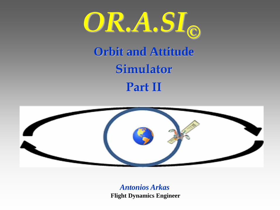
6. Celestial Events Module
6.1 Celestial Events Module Characteristics
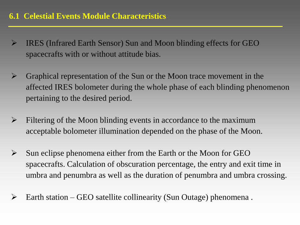
IRES (Infrared Earth Sensor) Sun and Moon blinding effects for GEO
spacecrafts with or without attitude bias.
Graphical representation of the Sun or the Moon trace movement in the
affected IRES bolometer during the whole phase of each blinding phenomenon
pertaining to the desired period.
Filtering of the Moon blinding events in accordance to the maximum
acceptable bolometer illumination depended on the phase of the Moon.
Sun eclipse phenomena either from the Earth or the Moon for GEO
spacecrafts. Calculation of obscuration percentage, the entry and exit time in
umbra and penumbra as well as the duration of penumbra and umbra crossing.
Earth station – GEO satellite collinearity (Sun Outage) phenomena .
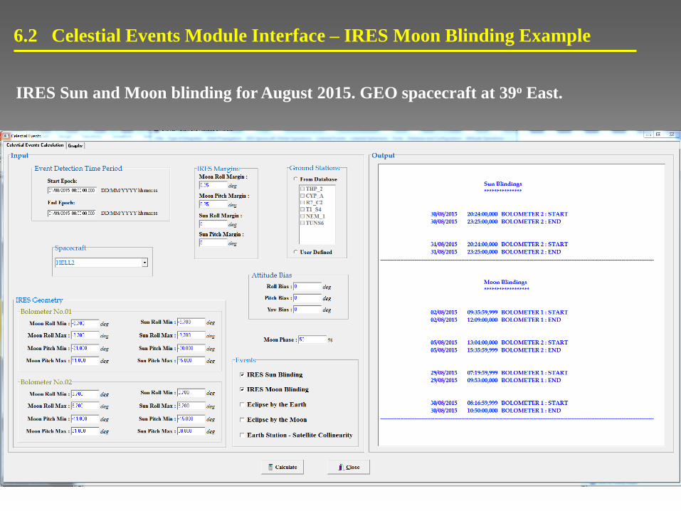
6.2 Celestial Events Module Interface – IRES Moon Blinding Example
IRES Sun and Moon blinding for August 2015. GEO spacecraft at 39o East.

6.3 IRES Moon Blinding- Validation with FocusGEO (GMV)
IRES Moon blinding for August 2015. GEO spacecraft at 39o East.
FocusGEO
OR.A.SI©
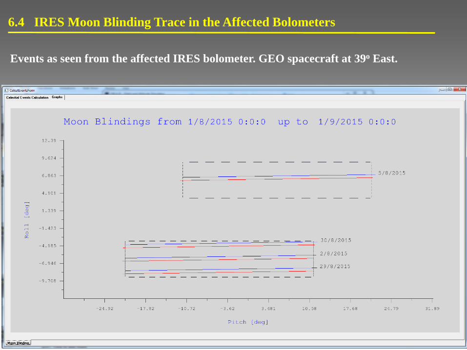
6.4 IRES Moon Blinding Trace in the Affected Bolometers
Events as seen from the affected IRES bolometer. GEO spacecraft at 39o East.
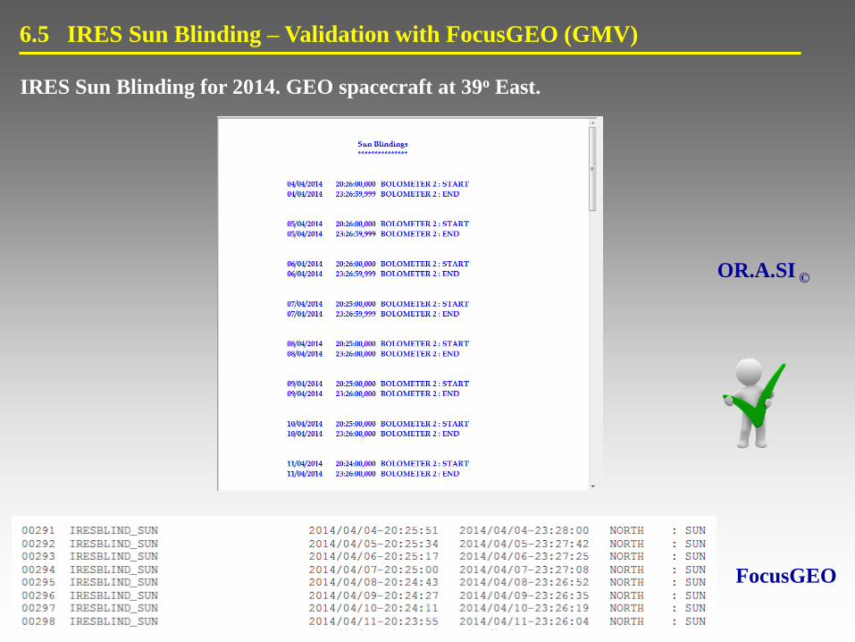
6.5 IRES Sun Blinding – Validation with FocusGEO (GMV)
IRES Sun Blinding for 2014. GEO spacecraft at 39o East.
OR.A.SI ©
FocusGEO

6.6 IRES Sun Blinding Graph
GEO spacecraft at 39o East. Events as seen from the affected IRES bolometer.

6.7 Sun Eclipse by the Moon –Validation with FocusGEO (GMV)
Events for 2014. GEO spacecraft at 39o East.
OR.A.SI ©
FocusGEO

6.7 Sun Eclipse by the Earth – Validation with COSMIC (AIRBUS)
Spring eclipse for 2011. GEO spacecraft at 39o East.
OR.A.SI © COSMIC
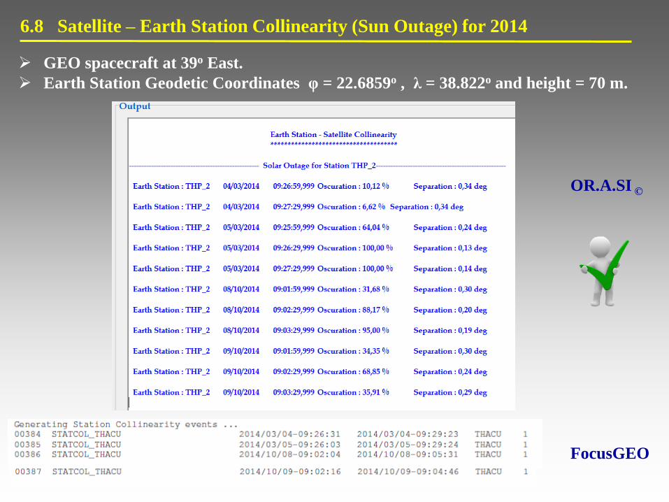
6.8 Satellite – Earth Station Collinearity (Sun Outage) for 2014
GEO spacecraft at 39o East.
Earth Station Geodetic Coordinates φ = 22.6859o , λ = 38.822o and height = 70 m.
OR.A.SI ©
FocusGEO

7. GEO Mission Analysis Module

Orbit
Propagation
Station Keeping
Maneuver
Calculation
Maneuver
Execution With
Gaussian Errors
Simulation of Tracking
Measurements With Noise
7.1 Integration of OR.A.SI© Modules for Mission Analysis Purposes
Ergol
Consumption Simulation of Tracking
Measurements With
Noise
Mission Analysis
Cycle
Orbit
Determination Orbit
Determination

7.2 Mission Analysis Module Characteristics
Consecutive mission analysis for more than one GEO spacecrafts and computation of
their intersatellite characteristics for each pair of them.
Realization of different station keeping strategy for each participating spacecraft
through the definition of the following parameters:
• Station keeping cycle duration.
• Inclination and drift/eccentricity control maneuver dates.
• Initiation of inclined orbit strategy after a desired date.
• Percentage of solar perturbation correction for the inclination control
maneuvers.
• Simulation of triaxial inclination control maneuver whose triaxiality is defined
from a different flat ACII file for each spacecraft.
• Calculation of inclination control maneuvers based either on correction of
secular drift or optimized long term strategy (E.M.Soop).
Automatic initial state vector computation for each spacecraft in accordance to the
desired station keeping strategy.
Production of localization measurements with Gaussian distributed errors.
Orbit determination based on erroneous measurement production.
Maneuver calculation based on the outcome of the orbit determination.
Addition of Gaussian maneuver execution errors.
Calculation of ergol consumption based on the Isp of each spacecraft.
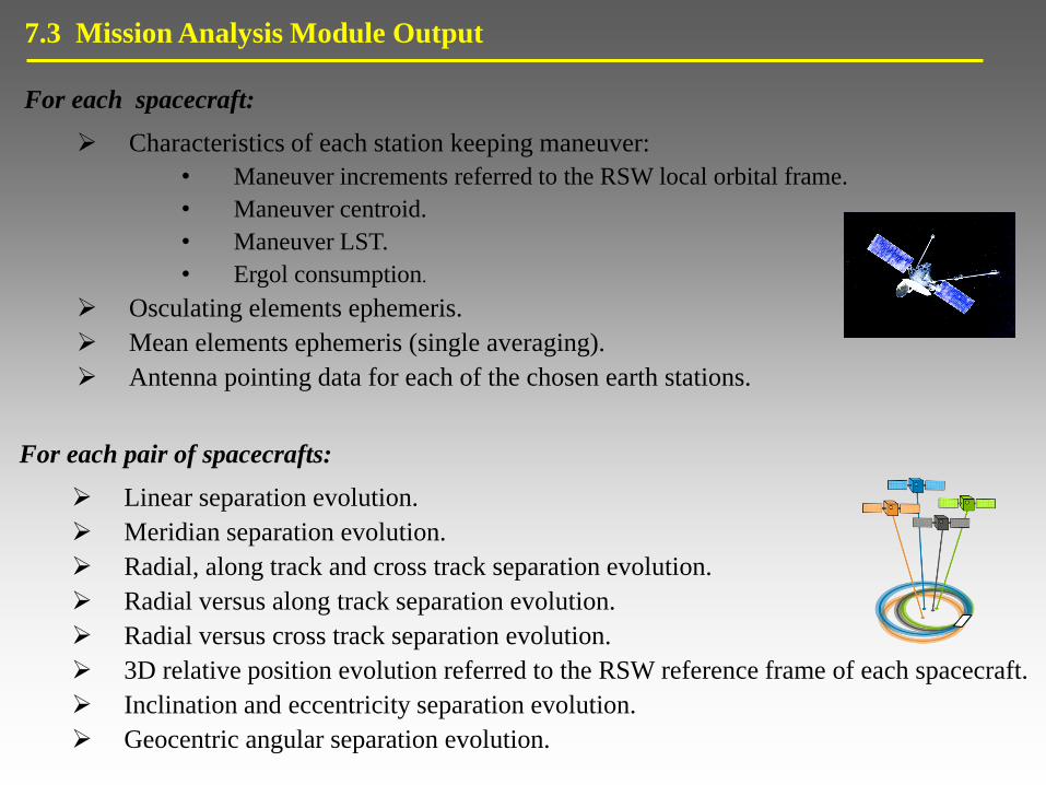
7.3 Mission Analysis Module Output
For each spacecraft:
Characteristics of each station keeping maneuver:
• Maneuver increments referred to the RSW local orbital frame.
• Maneuver centroid.
• Maneuver LST.
• Ergol consumption.
Osculating elements ephemeris.
Mean elements ephemeris (single averaging).
Antenna pointing data for each of the chosen earth stations.
For each pair of spacecrafts:
Linear separation evolution.
Meridian separation evolution.
Radial, along track and cross track separation evolution.
Radial versus along track separation evolution.
Radial versus cross track separation evolution.
3D relative position evolution referred to the RSW reference frame of each spacecraft.
Inclination and eccentricity separation evolution.
Geocentric angular separation evolution.
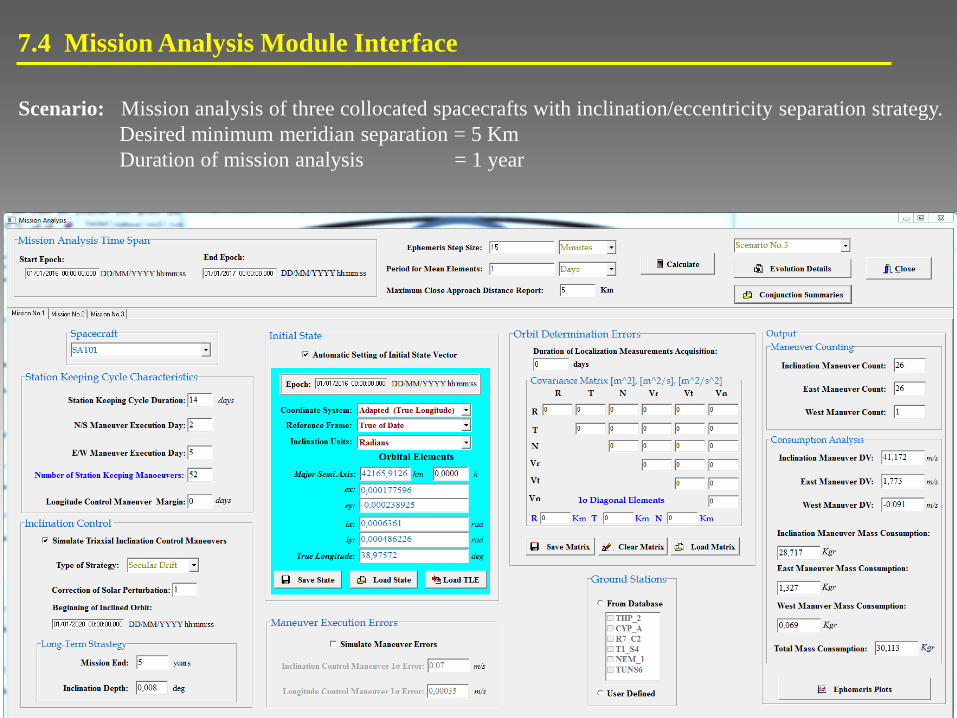
7.4 Mission Analysis Module Interface
Scenario: Mission analysis of three collocated spacecrafts with inclination/eccentricity separation strategy.
Desired minimum meridian separation = 5 Km
Duration of mission analysis = 1 year
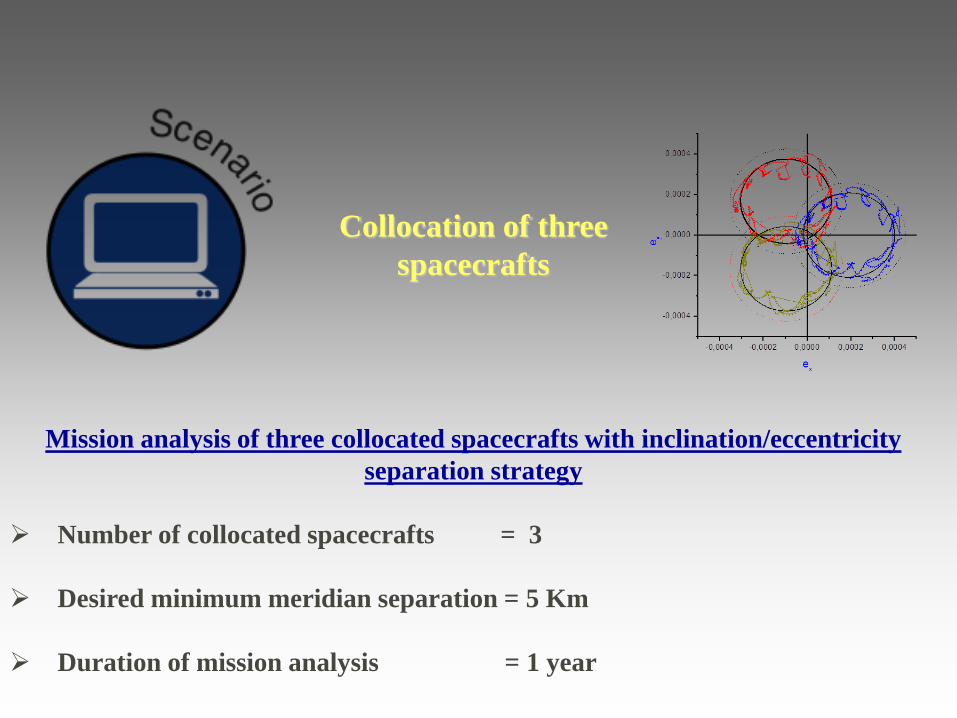
Mission analysis of three collocated spacecrafts with inclination/eccentricity
separation strategy
Number of collocated spacecrafts = 3
Desired minimum meridian separation = 5 Km
Duration of mission analysis = 1 year
Collocation of three
spacecrafts

Inclination-Eccentricity Separation Characteristics
Desired Characteristics for Collocated Spacecrafts
• Number of spacecrafts : 3
• Minimum distance : 5 km
• Station keeping cycle : 14 days
• Nominal longitude : 39.0o East
• Longitude window semi-dimension : 0.09o
• Maximum eccentricity : 4.0e-4
• Maximum latitude : 0.05o
• Eccentricity tolerance : 5.0e-5 0
0.034542
0.000237
o
ie
i
e
Separation Parameters
Characteristics of Inclination and Eccentricity Polygons

Inclination-Eccentricity Configuration

Inclination-Eccentricity Biases for Each Collocated Spacecraft

Single Satellite Plots – Evolution of Osculating and Mean Major Semi Axis
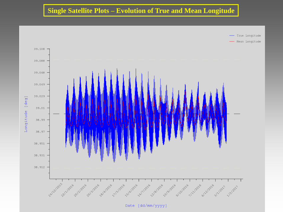
Single Satellite Plots – Evolution of True and Mean Longitude

Single Satellite Plots – Evolution of Osculating and Mean Eccentricity

One Year Inclination Evolution for Each Pair of Collocated Spacecrafts
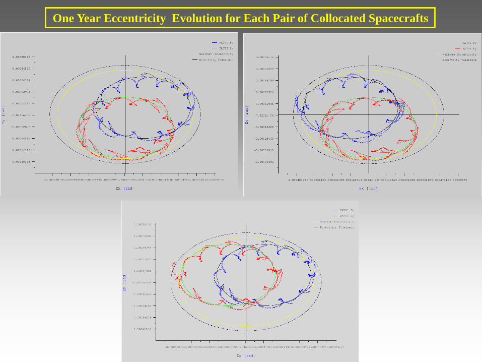
One Year Eccentricity Evolution for Each Pair of Collocated Spacecrafts
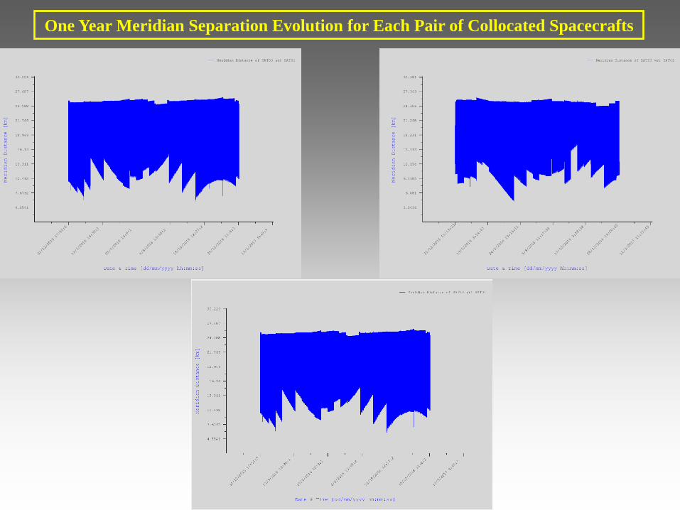
One Year Meridian Separation Evolution for Each Pair of Collocated Spacecrafts
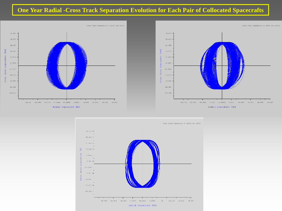
One Year Radial -Cross Track Separation Evolution for Each Pair of Collocated Spacecrafts
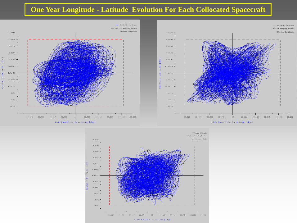
One Year Longitude - Latitude Evolution For Each Collocated Spacecraft
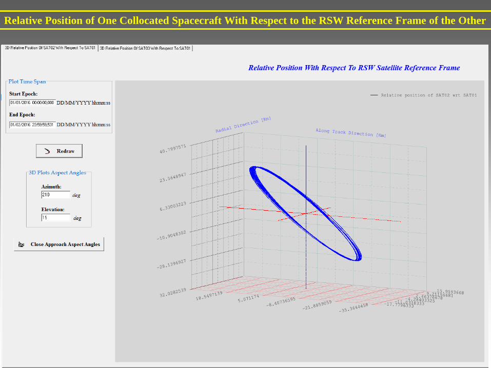
Relative Position of One Collocated Spacecraft With Respect to the RSW Reference Frame of the Other
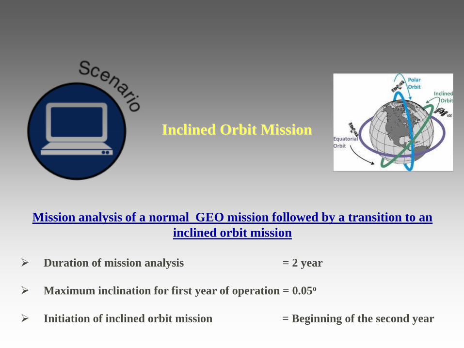
Mission analysis of a normal GEO mission followed by a transition to an
inclined orbit mission
Duration of mission analysis = 2 year
Maximum inclination for first year of operation = 0.05o
Initiation of inclined orbit mission = Beginning of the second year
Inclined Orbit Mission

Osculating and Mean Inclination Evolution

Geodetic Latitude versus Sub-satellite Longitude
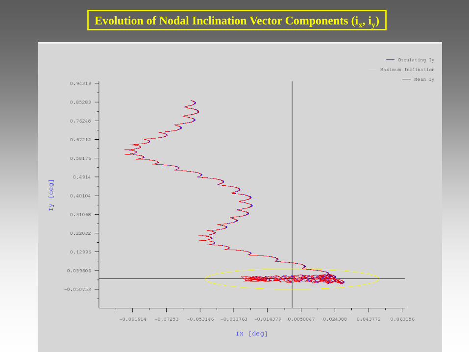
Evolution of Nodal Inclination Vector Components (ix, iy)
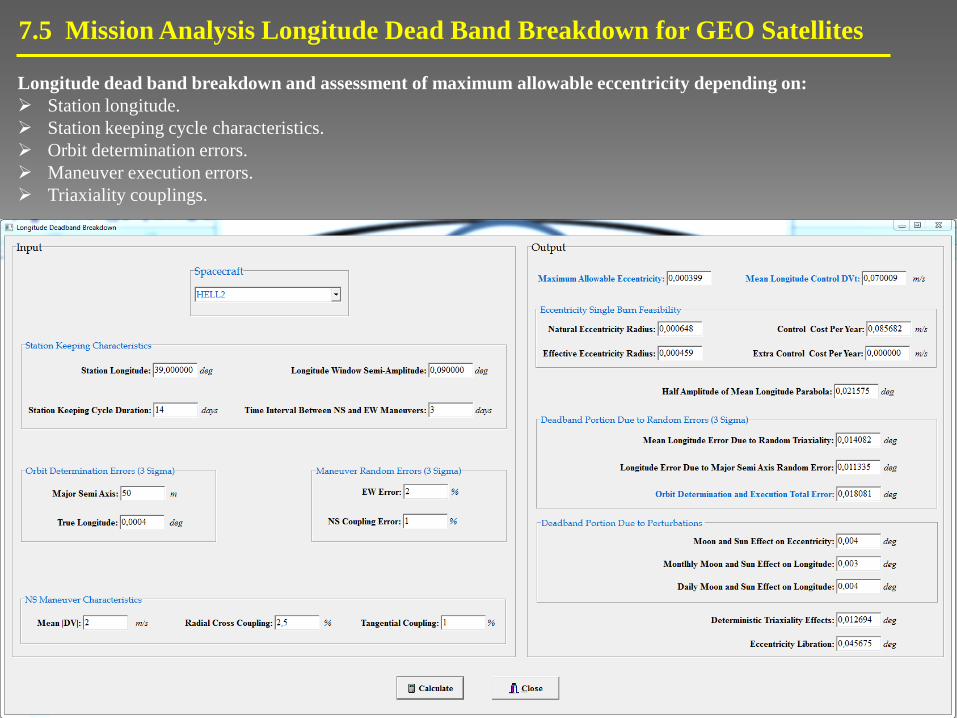
7.5 Mission Analysis Longitude Dead Band Breakdown for GEO Satellites
Longitude dead band breakdown and assessment of maximum allowable eccentricity depending on:
Station longitude.
Station keeping cycle characteristics.
Orbit determination errors.
Maneuver execution errors.
Triaxiality couplings.
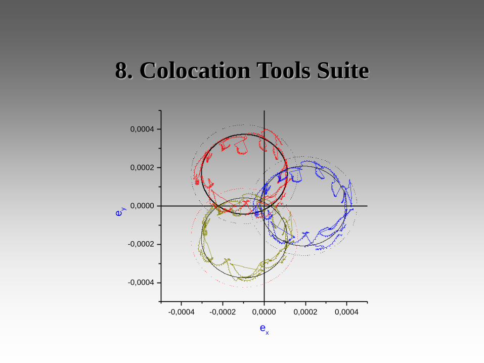
8. Colocation Tools Suite
-0,0004 -0,0002 0,0000 0,0002 0,0004
-0,0004
-0,0002
0,0000
0,0002
0,0004
ey
ex

Computation of the characteristics of the colocation configuration (inclination
separation, eccentricity separation, inclination control radius, eccentricity control radius,
inclination and eccentricity biases) corresponding to a desired minimum separation,
number of spacecrafts, maximum eccentricity and maximum inclination for the
colocation cluster.
Flexibility to compute colocation configuration with arbitrarily rotated regular polygons
in the inclination node vector space (rotation with respect to contemporary secular drift
direction) and in the eccentricity vector space (rotation with respect to the inclination
regular polygon).
Assessment of the safety of the chosen minimum separation by comparing it with the
worst case combined covariance matrix of the relative position of the collocated pair of
spacecrafts, which takes account both the orbit determination and the maneuver
execution errors (retrieved from the database containing the spacecraft characteristics).
Simulation of the computed configuration with mission analysis module and
computation of all the relevant intersatellite characteristics.
8.1 Colocation Initialization Tool Characteristics

8.2 Colocation Initialization Tool Interface
Scenario: Colocation of 5 spacecrafts with desired minimum separation 5 Km.
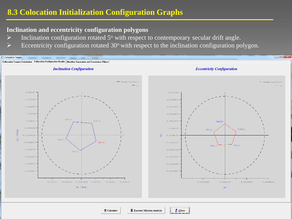
8.3 Colocation Initialization Configuration Graphs
Inclination and eccentricity configuration polygons
Inclination configuration rotated 5o with respect to contemporary secular drift angle.
Eccentricity configuration rotated 30o with respect to the inclination configuration polygon.
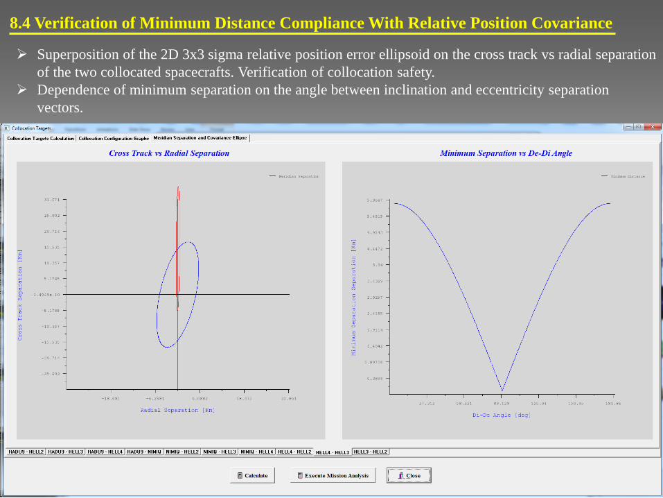
8.4 Verification of Minimum Distance Compliance With Relative Position Covariance
Superposition of the 2D 3x3 sigma relative position error ellipsoid on the cross track vs radial separation
of the two collocated spacecrafts. Verification of collocation safety.
Dependence of minimum separation on the angle between inclination and eccentricity separation
vectors.

9. Monte Carlo
Verification of Colocation
Configuration

Verification of the collocation configuration conformity with the desired minimum linear
separation through the computation of the minimum linear separation and minimum
meridian separation with Monte Carlo method.
Flexibility to execute Monte Carlo simulation for two spacecrafts whose station keeping
cycles are either non synchronized (random number of days between the beginning of
their station keeping cycles) or for spacecrafts with specific time difference between
their maneuver execution dates.
Simulation of the impact of inclination control maneuver abort and of orbit
determination errors.
Computation of the 3x3σ relative separation statistics based on the propagation of the
combined covariance matrix of the relative position of the collocated spacecrafts.
Realistic propagation of combined position covariance by taking account the
initialization impact of orbit determination on the covariance of each spacecraft.
9.1 Monte Carlo Collocation Tool Characteristics
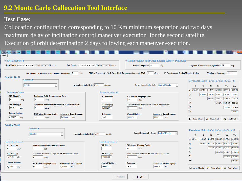
9.2 Monte Carlo Collocation Tool Interface
Test Case:
Collocation configuration corresponding to 10 Km minimum separation and two days
maximum delay of inclination control maneuver execution for the second satellite.
Execution of orbit determination 2 days following each maneuver execution.
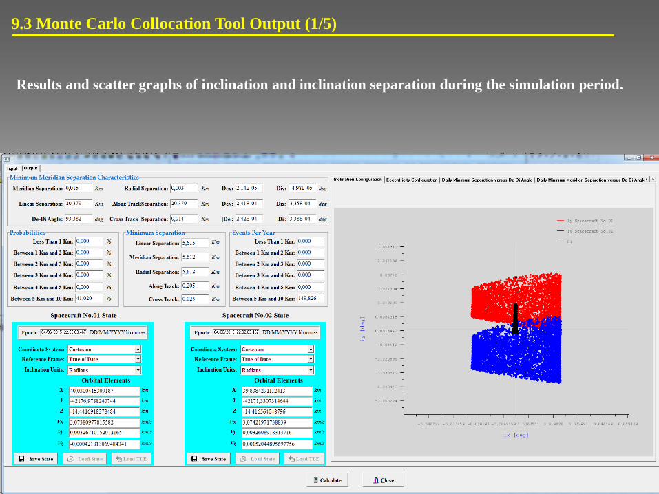
9.3 Monte Carlo Collocation Tool Output (1/5)
Results and scatter graphs of inclination and inclination separation during the simulation period.

9.3 Monte Carlo Collocation Tool Output (2/5)
Results and scatter graphs of eccentricity and eccentricity separation during the simulation period.
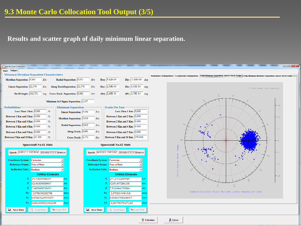
9.3 Monte Carlo Collocation Tool Output (3/5)
Results and scatter graph of daily minimum linear separation.
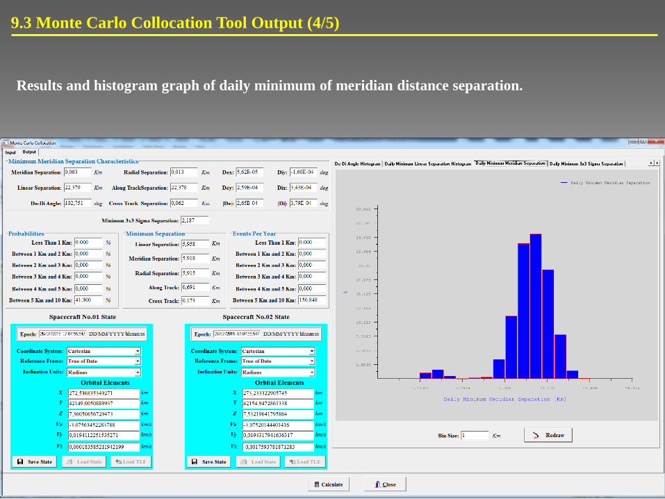
9.3 Monte Carlo Collocation Tool Output (4/5)
Results and histogram graph of daily minimum of meridian distance separation.

9.3 Monte Carlo Collocation Tool Output (5/5)
Results and histogram graph of daily minimum of 3x3 sigma separation d= ∆𝒓𝟐𝒊∆𝝈𝟐𝒊
𝟑𝒊=𝟏
where ri are the components of the separation vector towards the principal directions of the relative
position ellipsoid and σi the corresponding semi-axes lengths.

10. Close Approach Detection

Utilization of Hoots prefilters (perigee-apogee, geometric, time and coplanar
prefilters) for the efficient scanning of the whole TLE catalogue released from
NORAD and detection of close approach events for a desired primary object.
Detection of consecutive close approach events both for primary objects whose
state is described by a TLE and for maneuverable objects whose state during the
filtering period is given by the initial state of the primary object and the planned
orbital maneuvers to be executed during this period.
Confirmation of each close approach event with subsequent computation of the
minimum distance with numerical propagation of both primary and secondary
(intruder) objects.
Direct validation of module with actual Conjunction Reports sent by SDA.
10.1 Close Approach Early Warning Module Based On An Analytic Method
Algorithm based on the paper: An Analytic Method to Detect Future Close Approaches Between Satellites
by Felix R.Hoots, Linda L.Crawford, and Ronald L. Roehrich

10.2 Close Approach Early Warning Interface
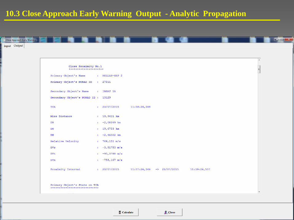
10.3 Close Approach Early Warning Output - Analytic Propagation

13.4 Close Approach Early Warning Output - Numerical Propagation
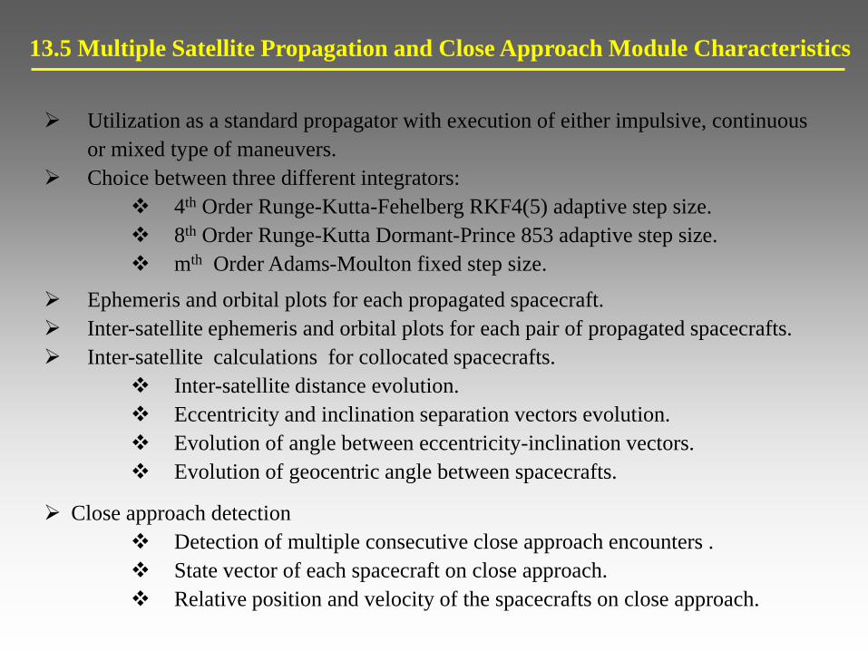
Utilization as a standard propagator with execution of either impulsive, continuous
or mixed type of maneuvers.
Choice between three different integrators:
4th Order Runge-Kutta-Fehelberg RKF4(5) adaptive step size.
8th Order Runge-Kutta Dormant-Prince 853 adaptive step size.
mth Order Adams-Moulton fixed step size.
Ephemeris and orbital plots for each propagated spacecraft.
Inter-satellite ephemeris and orbital plots for each pair of propagated spacecrafts.
Inter-satellite calculations for collocated spacecrafts.
Inter-satellite distance evolution.
Eccentricity and inclination separation vectors evolution.
Evolution of angle between eccentricity-inclination vectors.
Evolution of geocentric angle between spacecrafts.
Close approach detection
Detection of multiple consecutive close approach encounters .
State vector of each spacecraft on close approach.
Relative position and velocity of the spacecrafts on close approach.
13.5 Multiple Satellite Propagation and Close Approach Module Characteristics
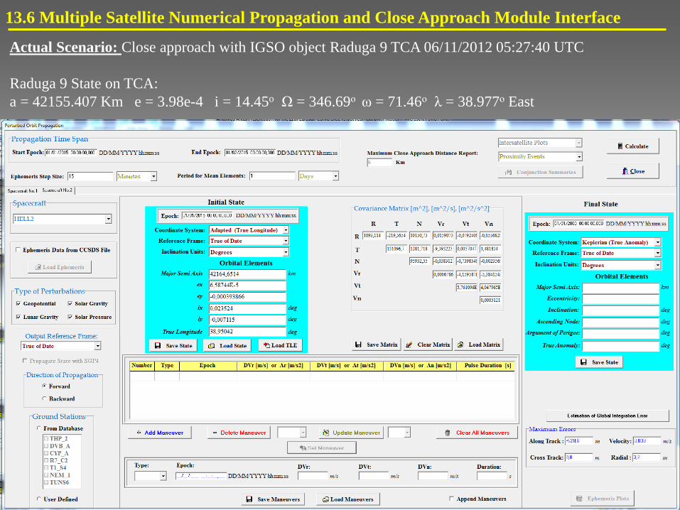
13.6 Multiple Satellite Numerical Propagation and Close Approach Module Interface
Actual Scenario: Close approach with IGSO object Raduga 9 TCA 06/11/2012 05:27:40 UTC
Raduga 9 State on TCA:
a = 42155.407 Km e = 3.98e-4 i = 14.45o Ω = 346.69ο ω = 71.46ο λ = 38.977ο East
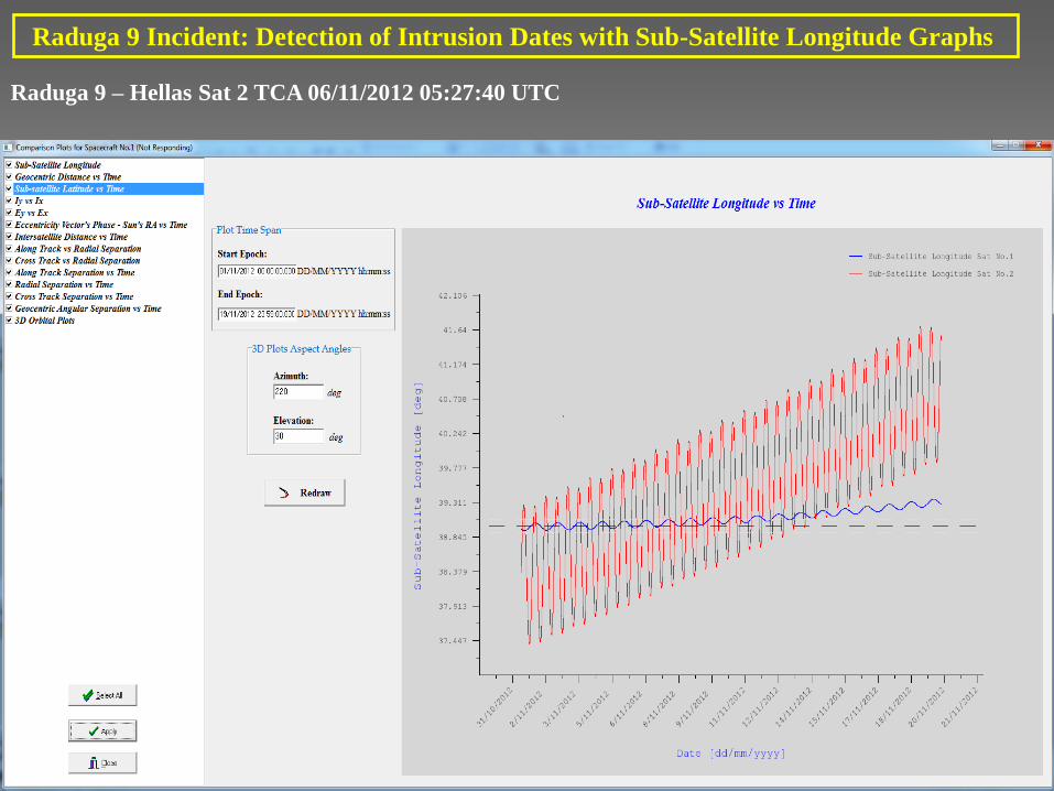
Raduga 9 Incident: Detection of Intrusion Dates with Sub-Satellite Longitude Graphs
Raduga 9 – Hellas Sat 2 TCA 06/11/2012 05:27:40 UTC

Raduga 9 Incident: Detection of Consecutive Close Encounters with Inter-satellite Distance Graphs
Raduga 9 – Hellas Sat 2 TCA 06/11/2012 05:27:40 UTC
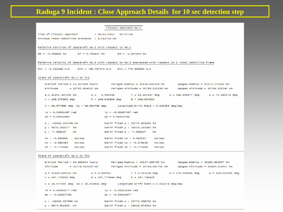
Raduga 9 Incident : Close Approach Details for 10 sec detection step

Raduga 9 Incident: 2 Years Long Term Libration Around A Stable Equilibrium Point
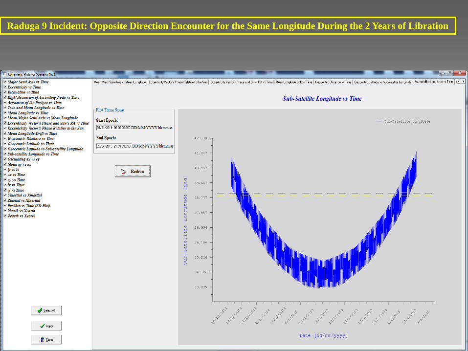
Raduga 9 Incident: Opposite Direction Encounter for the Same Longitude During the 2 Years of Libration

11. Collision Mitigation for
High Relative Velocity Encounters

All figure were borrowed from AIAA Paper 05-308 COLLISION AVOIDANCE MANEUVER PLANNING TOOL
by SALVATORE ALFANO
11.1 Geometry and Mathematics of High Relative Velocity Close Encounters (1/2)
Assumptions
Small encounter time to
ensure constancy of the
individual covariance
matrices and the resulting
combined covariance
matrix.
High relative velocity to
allow the reduction of the
3D integral to a 2D one.

11.2 Geometry and Mathematics of High Relative Velocity Close Encounters (2/2)
Maximum probability Pmax corresponds
to xm=0 and a specific minor semi axis of
combined covariance ellipse.
The probability dilution region is that
region where the standard deviation of
the combined covariance minor semi
axis σx exceeds that which yield Pmax.
If operating within the dilution region,
then the further into this region the
uncertainty progresses the more
unreasonable it becomes to associate low
probability with low risk.
Two-dimensional probability equation in the encounter plane: • OBJ - Combined object radius.
• σx - Projected covariance ellipse
minor semi axis.
• σy - Projected covariance ellipse
major semi axis.
• (xm ,ym) - Projection of miss distance
on covariance frame.

11.3 Collision Mitigation Module Characteristics
Accurate calculation of close approach characteristics (depended on detection step size):
Miss distance on TCA (Time of Closest Approach).
Relative position and velocity of secondary object with respect to primary object
on TCA.
State vector details of both primary and secondary objects on TCA.
Collision probability assessment.
Collision probability based on combined covariance.
Maximum collision probability for unfavorable orientation and size of the
combined covariance ellipsoid.
Calculation of probability dilution region.
Characteristics of the combined error ellipsoid and its projection on the conjunction
plane (combined covariance ellipse)
Design and optimality testing of along track (East-West) avoidance maneuvers for a
desired range of DVs.
Collision probability following the execution of each avoidance maneuver .
Miss distance following the execution of each avoidance maneuver
Longitude window violation details corresponding to desired avoidance maneuver.
Monte Carlo simulation of spacecraft collision with or without avoidance maneuver.
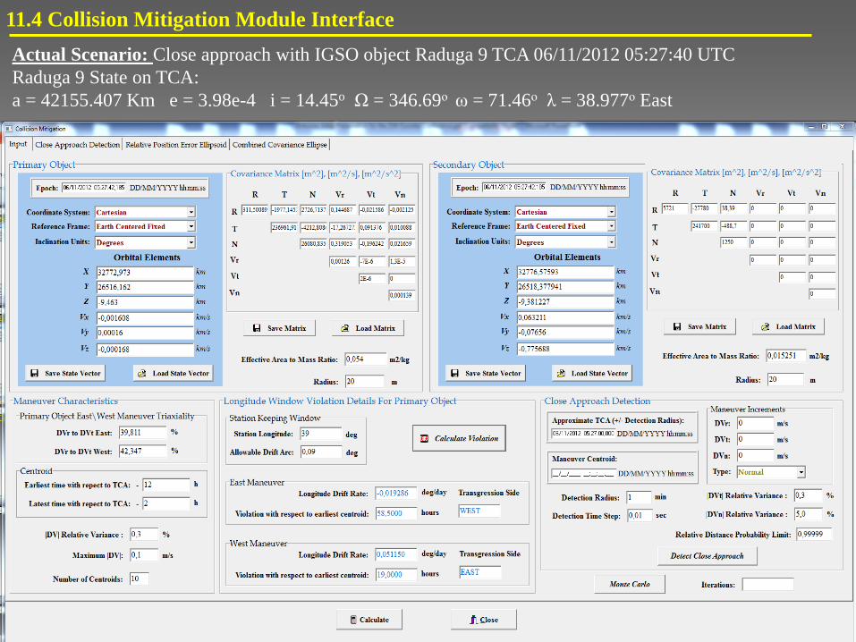
11.4 Collision Mitigation Module Interface
Actual Scenario: Close approach with IGSO object Raduga 9 TCA 06/11/2012 05:27:40 UTC
Raduga 9 State on TCA:
a = 42155.407 Km e = 3.98e-4 i = 14.45o Ω = 346.69ο ω = 71.46ο λ = 38.977ο East

11.5 Validation of Miss Distance and Relative Position -Velocity Calculations With JSpOC CSM

Combined Covariance Ellipsoid Characteristics Referred to the Axes Defined by the Relative Velocity
Vector, the Line of Sight of the Two Objects on TCA (which is perpendicular to relative velocity
vector) and a Direction Normal to the Plane Defined by the Other Two Axes

Projection of Combined Covariance
Ellipse on Encounter Plane and
Orientation of Line of Sight on TCS
Dependence of Collision Probability on the
Orientation of Line of Sight With Respect
to the Combined Covariance Ellipse

11.6 Why Probability Calculations are Much Safer than Miss Distance for
Collision Mitigation Decision Making (1/2)
Close Approach Scenario for Miss Distance 1.166 Km and P = 5E-08
Miss Distance – Relative Position – Relative Velocity – Collision Probability

11.7 Why Probability Calculations are Much Safer than Miss Distance for
Collision Mitigation Decision Making (2/2)
Dependence of collision probability on relative position of spacecraft line of sight, on TCA, with respect to combined covariance ellipse

11.8 Validation for Collision Probability P = 0.0164 in the Dilution Region (1/2)
Close Approach Scenario
Miss Distance – Relative Position – Relative Velocity – Collision Probability

0 20000 40000 60000 80000 100000 120000
0,010
0,012
0,014
0,016
0,018
0,020
Coll
isio
n P
robab
ilit
y
Number of Monte Carlo Iterations
Collision Probability
Monte Carlo Convergence of Collision Probability
• Theoretical : 0.01645
• Monte Carlo : 0.01639 (121846 iterations)
11.9 Validation for Collision Probability P = 0.0164 in the Dilution Region (2/2)

What is the latest time with respect to
TCA when a moderate (~ 0.04 m/s)
avoidance maneuver is able to
substantially decrease the collision
probability ?
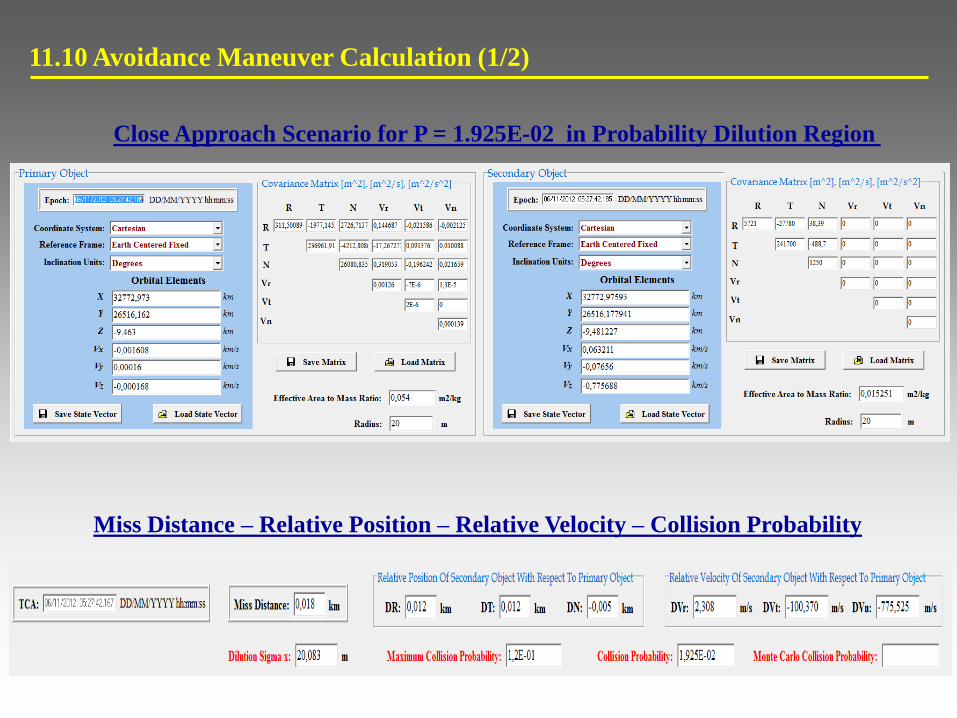
11.10 Avoidance Maneuver Calculation (1/2)
Close Approach Scenario for P = 1.925E-02 in Probability Dilution Region
Miss Distance – Relative Position – Relative Velocity – Collision Probability
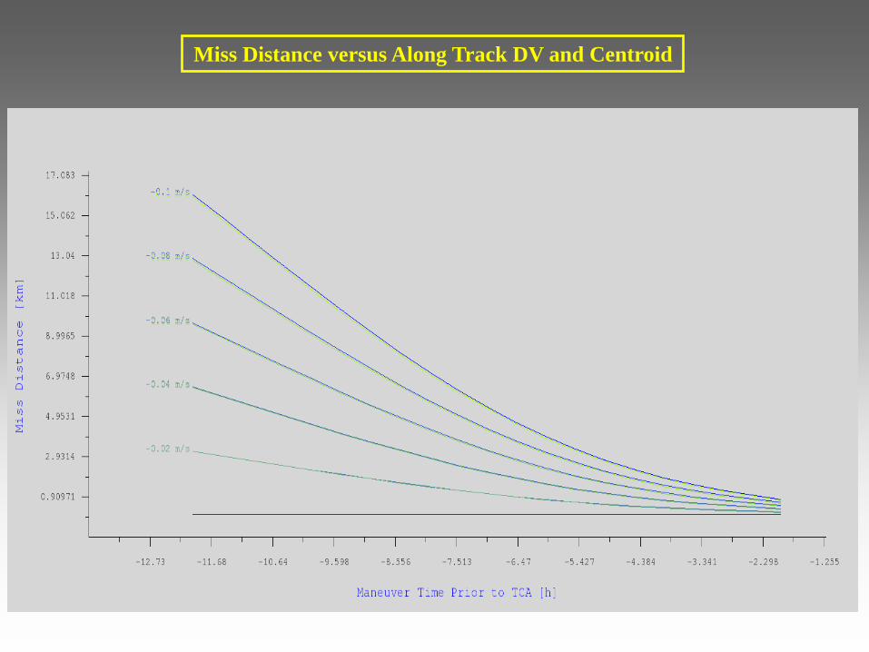
Miss Distance versus Along Track DV and Centroid

Collision Probability versus Along Track DV and Centroid

11.11 Validation of Collision Mitigation with an Avoidance Maneuver
Collision Probability without Avoidance Maneuver : 1.93E-02
• Theoretical : 1.95E-06 (Probability Dilution)
• Monte Carlo : 2.5E-06 (2 million iterations)
Collision Probability with a 0.04 m/s maneuver 2h prior to TCA

How much does the collision probability
depend on state covariance matrix
norm ?
or else
How strong does the collision probability
depend on observability ?
or else
Can a specific choice of orbit
determination setup reduce the
collision probability ?

11.12 Collision Probability and Observability
Collision probability can be substantially decreased by selecting the orbit
determination setup characterized from the best observability with respect to all
the possible allowable setups.
Best case primary
object’s state
covariance
Worst case primary
object’s state
covariance
Best case state covariance (Best Observability)
Worst case state covariance (Worst Observability)

Best case state
covariance
Dependence of Combined Covariance Ellipsoid Size on Individual Covariance Ellipsoids
Miss Distance : 1.166 Km
Worst case state
covariance

11.13 Characteristic Run-Time for Close Approach Calculations
Machine Used for OR.A.SI© Execution : Laptop with Intel i7 Processor and 2GB RAM
Preliminary Detection of Close Approach with Multiple Satellite Propagation
and Close Approach Module
• Detection period : 20 days
• Ephemeris Time Step : 1 min
• Propagator : 8th order Adams-Moulton
Run-Time: 22 sec
Accurate Detection of Close Approach with Collision Mitigation Module
• Detection Time Step : 0.01 sec
• Propagator : 8th order Adams-Moulton Run-Time: 6 sec
Avoidance Maneuver Calculation with Collision Mitigation Module
• Detection Time Step : 0.01 sec
• Number of Different Maneuver DV’s : 10
• Number of Centroids for Each DV : 20
• Total Avoidance Maneuver Number : 200
• Propagator : 8th order Adams-Moulton
Run-Time: 3 min 33sec
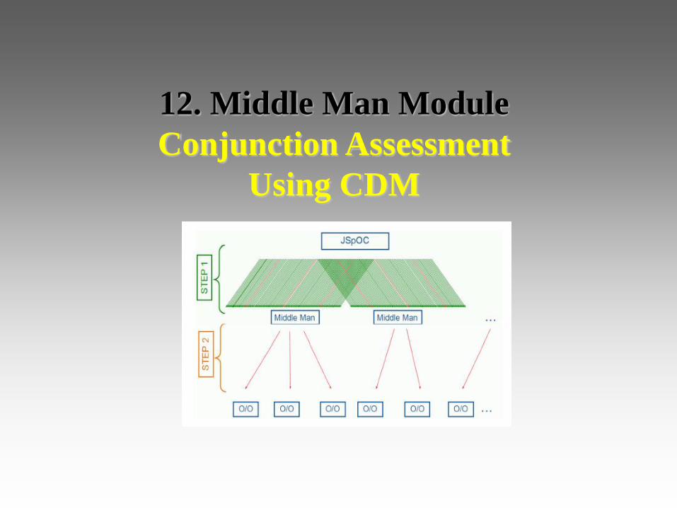
12. Middle Man Module
Conjunction Assessment
Using CDM
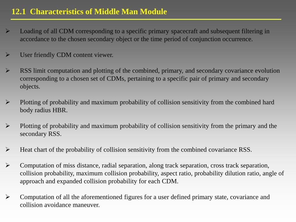
12.1 Characteristics of Middle Man Module
Loading of all CDM corresponding to a specific primary spacecraft and subsequent filtering in
accordance to the chosen secondary object or the time period of conjunction occurrence.
User friendly CDM content viewer.
RSS limit computation and plotting of the combined, primary, and secondary covariance evolution
corresponding to a chosen set of CDMs, pertaining to a specific pair of primary and secondary
objects.
Plotting of probability and maximum probability of collision sensitivity from the combined hard
body radius HBR.
Plotting of probability and maximum probability of collision sensitivity from the primary and the
secondary RSS.
Heat chart of the probability of collision sensitivity from the combined covariance RSS.
Computation of miss distance, radial separation, along track separation, cross track separation,
collision probability, maximum collision probability, aspect ratio, probability dilution ratio, angle of
approach and expanded collision probability for each CDM.
Computation of all the aforementioned figures for a user defined primary state, covariance and
collision avoidance maneuver.

12.2 CDM File Loader and Filtering

12.3 CDM Viewer

12.4 2D Combined Covariance and Projection of Minimum Separation Evolution
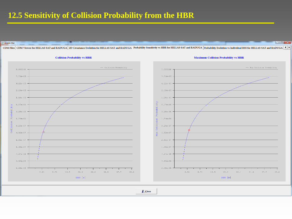
12.5 Sensitivity of Collision Probability from the HBR

12.6 Sensitivity of Collision Probability from Primary and Secondary RSS

12.7 Heat Chart for Probability of Collision Sensitivity from Combined RSS

13. Tools

13.1 Time Conversion Tool (Calendrical Calculations And Conversions)

Transformation between Keplerian elements (true anomaly- mean anomaly - true longitude – mean longitude),
Adapted elements (true longitude – mean longitude), ECI state vector and ECF state vector.
Transformation between reference frames (Mean of 1950, Mean of J2000, Mean of Date, True of Date and Veis).
Propagation of state prior to transformation.
13.2 State Transformation Tool (1/2)

Transformation from TLE to Keplerian elements (true anomaly- mean anomaly - true longitude – mean
longitude), Adapted elements (true longitude – mean longitude), ECI state vector and ECF state vector.
Transformation is done via the SGP4 model.
13.2 State Transformation Tool (2/2)

13.3 Earth Station – Satellite Geometry Calculations and Transformations
Transformation from topocentric horizon (range, azimuth elevation) to geodetic coordinates (height above reference
ellipsoid, longitude, geodetic latitude) and vice versa.
Antenna biases and weather conditions are taken account (local temperature, relative humidity and barometric
pressure).
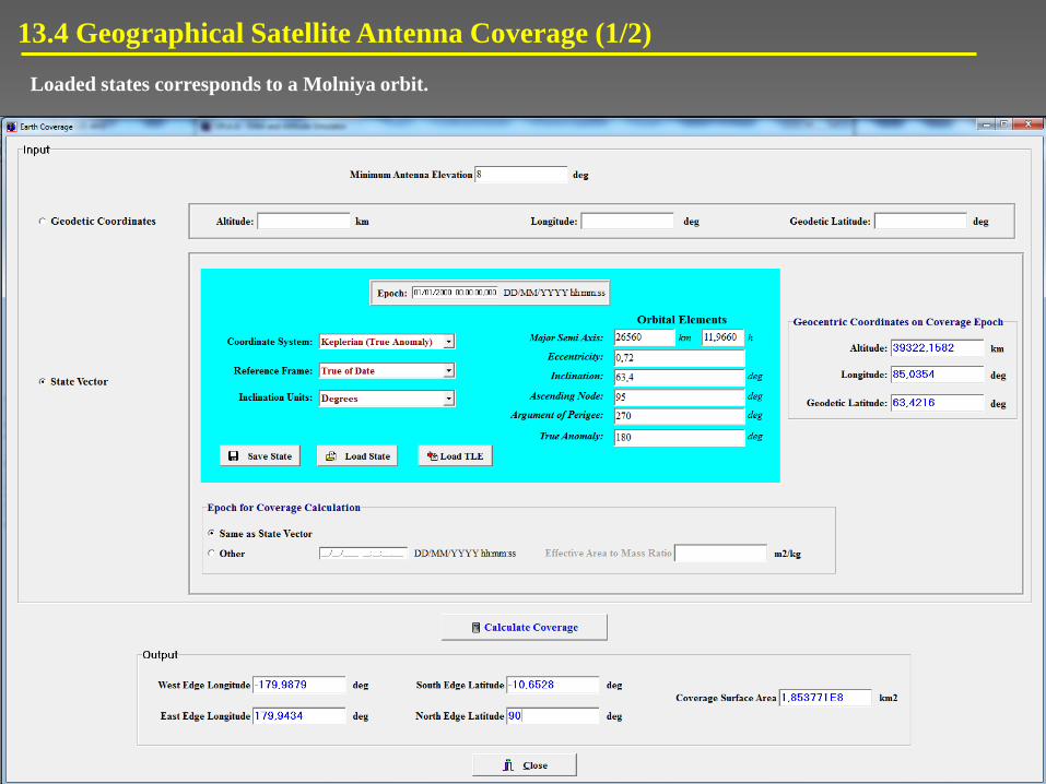
13.4 Geographical Satellite Antenna Coverage (1/2)
Loaded states corresponds to a Molniya orbit.
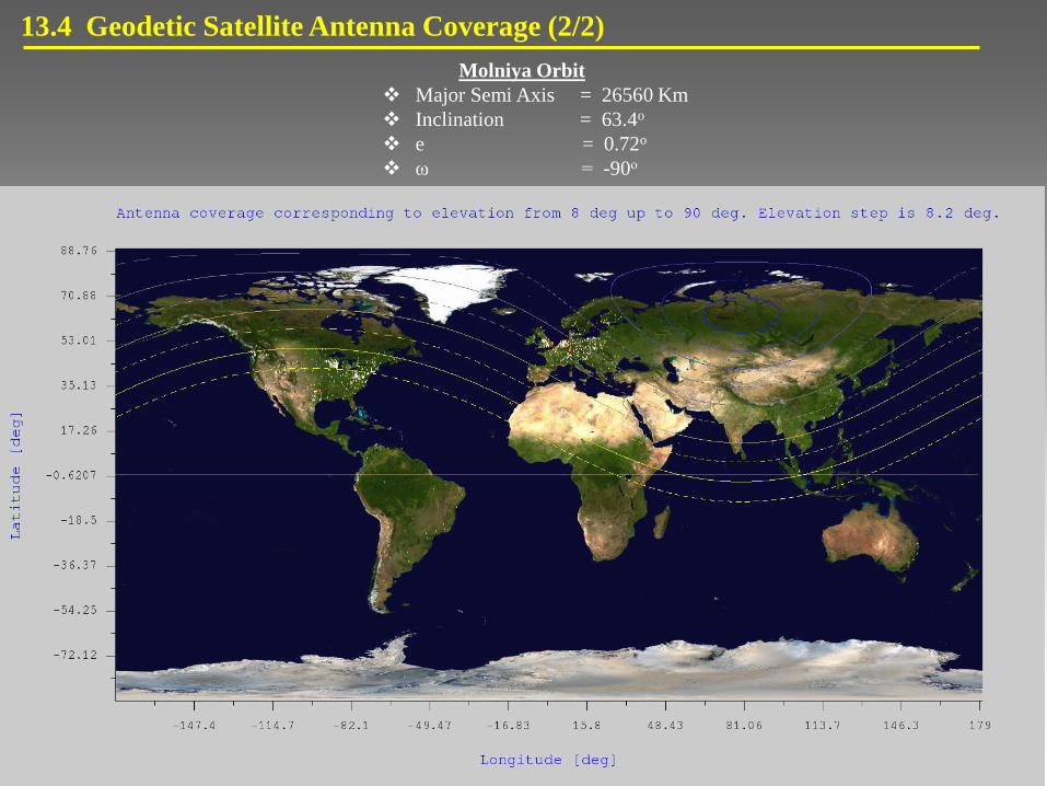
13.4 Geodetic Satellite Antenna Coverage (2/2)
Molniya Orbit
Major Semi Axis = 26560 Km
Inclination = 63.4o
e = 0.72o
ω = -90ο
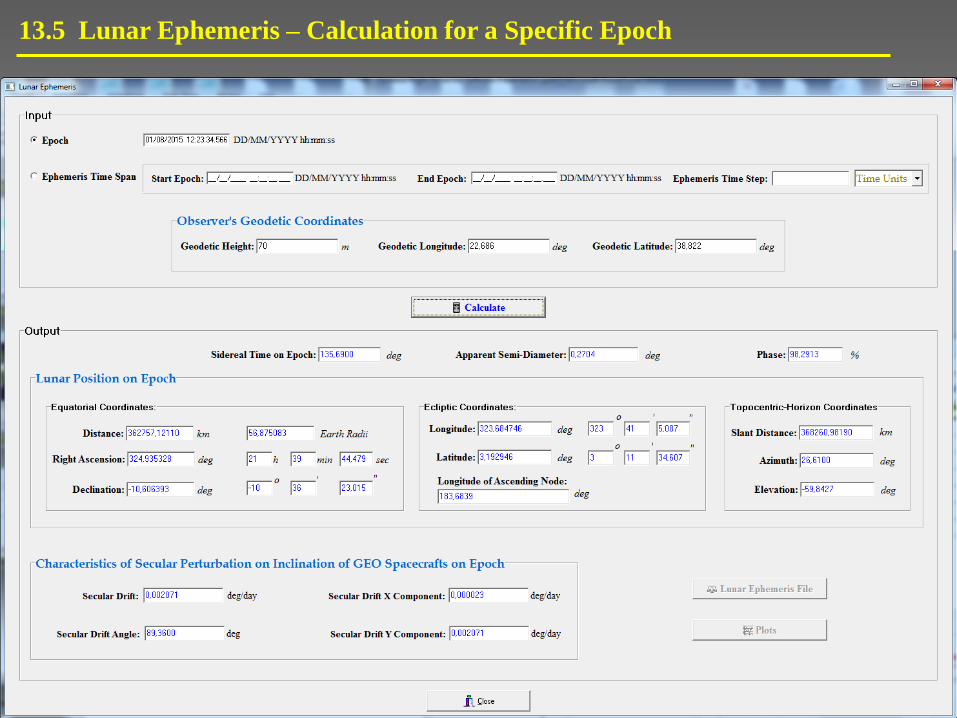
13.5 Lunar Ephemeris – Calculation for a Specific Epoch

13.6 Lunar Ephemeris – Calculation for a Time Period of 18.6 Years (1/2)
Evolution of GEO spacecrafts inclination secular drift modulus due to Lunar perturbation,
corresponding to a time period of 18.6 years.

13.7 Lunar Ephemeris – Calculation for a Time Period of 18.6 Years (2/2)
Evolution of GEO spacecrafts inclination secular drift angle due to Lunar perturbation, corresponding to a
time period of 18.6 years.

13.8 Solar Ephemeris – Calculation for a Specific Epoch (1/3)

13.8 Solar Ephemeris – Calculation for a Period of One Year (2/3)
Analemma plot.

13.8 Solar Ephemeris – Calculation for a Period of One Year (3/3)
Equation of time plot.

14. Database

14.1 Earth Station Database Interface
Database is structured on ASCII flat files.

14.2 Spacecraft Database Interface
15. Attitude Module
Characteristics
(Only in console GUI. Pending to be implemented in windows GUI)

15.1 Technical Features (1/3)
1. Numerical Integrator
Continuous embedded 6th stage Runge-Kutta-Fehelberg method RKF4(5)
Quaternions used as generalized coordinates (no problem with singular points and
instability cases).
2. Code capable of simulating the following rotational dynamic cases :
Free rigid body rotation.
Rotation of a rigid body under the influence of impulsive torques (thrusts).
Rotation of a rigid body under the influence of continuous torques (perturbing torques).
3. Motion description with respect to three different coordinate systems :
Quasi inertial reference frame MGSD – Mean Geocentric System of Date.
Body axis reference frame (sensors readings).
Local orbital frame.
4. Flexibility to initialize the rotational state of the spacecraft by defining :
The angular velocity vector with respect to any of the predefined coordinate systems.
The angular momentum vector with respect to any of the predefined coordinate systems.
The vector components form (Cartesian or Polar).

15.2 Technical Features (2/3)
5. Flexibility to describe the dynamical properties of the system to be
simulated :
Definition of the mass distribution by choosing the principal moments of inertia
Ixx , Iyy and Izz.
Addition of inertial wheels of whatever orientation by defining the respective
vector components of their angular momentum Lx, Ly and Lz with respect to the
body frame.
Model the behavior of a dual-spin satellite by identifying the platform with an
inertial wheel and the rotor with the rigid body.
6. Simultaneous description of the rotational motion by using four
different types of generalized coordinates :
Euler angles φ, θ and ψ (z-x-z convention).
Tait-Bryan angles (roll, pitch, yaw).
Directional cosines of the body axes with respect either to inertial or local frame.
Quaternions.
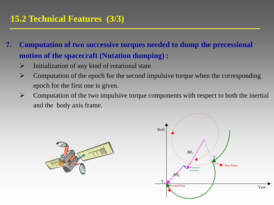
15.2 Technical Features (3/3)
7. Computation of two successive torques needed to dump the precessional
motion of the spacecraft (Nutation dumping) :
Initialization of any kind of rotational state.
Computation of the epoch for the second impulsive torque when the corresponding
epoch for the first one is given.
Computation of the two impulsive torque components with respect to both the inertial
and the body axis frame.
First Pulse
D 1
D H 2
T 1
2
Momentum
Precession
Roll
H
T Second Pulse Yaw

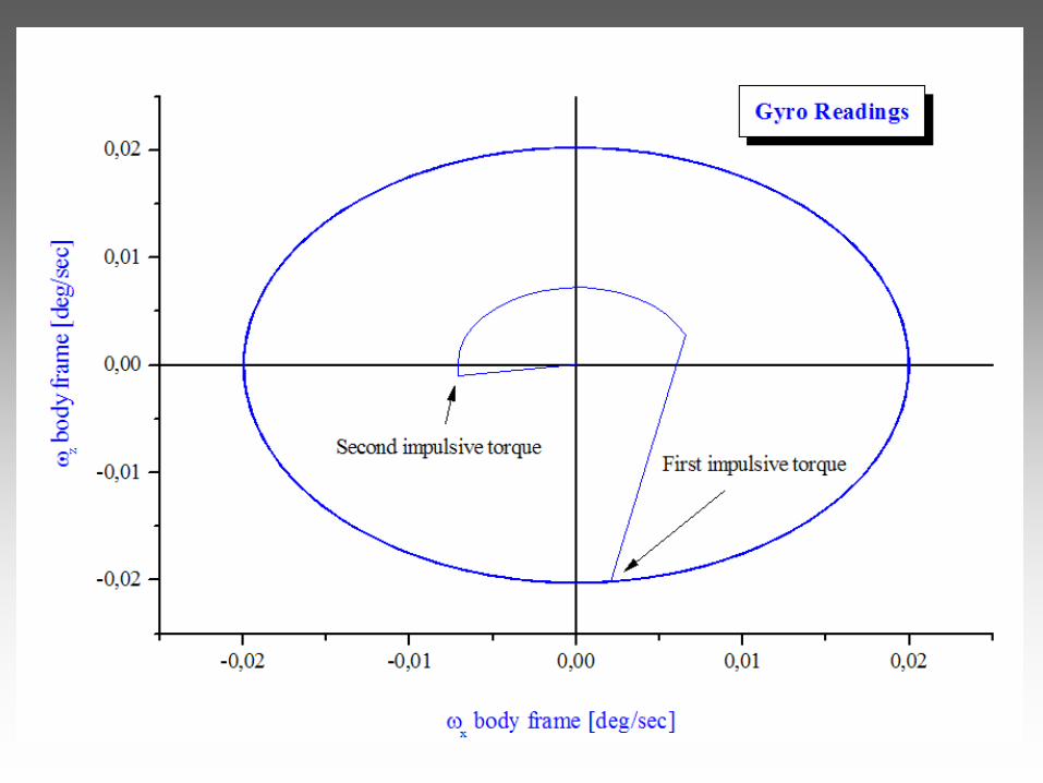
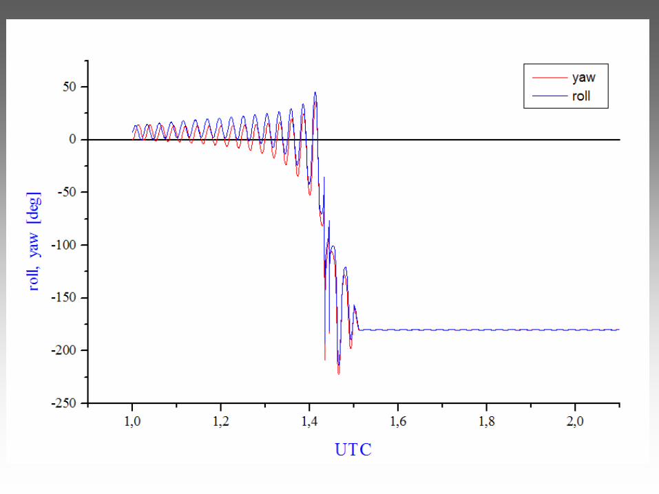
15.3 Output
UTC – Universal Time Coordinated
dd/mm/yyyy hh:mm:ss - Gregorian Date
GAST - Greenwich Apparent Sidereal
Time
Euler angles – φ,θ,ψ
Τait-Bryan angles – roll, pitch, yaw
Quaternions – qo, q1, q2, q3
Angular velocity with respect to the
inertial frame – ωx, ωy and ωz
Angular velocity ω with respect to the
body frame – Gyro readings.
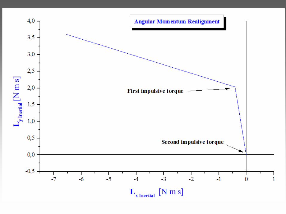
Angular momentum vector with respect
to inertial frame – Lx, Ly, Lz
Angular momentum vector with respect
to the body frame.
Angular momentum vector with respect
to the local orbital frame.
Directional cosines of the body axes
with respect to the inertial frame.
Directional cosines of the body axes
with respect to the local orbital frame.
Angle between the x,z and y body axes
and the angular momentum vector.
Angle between the angular velocity
vector and the angular momentum
vector.
LIASS unbalance angle.
LIASS pitch angle.

16. OR.A.SI Utilization for
Modeling Realistic
Attitude Problems

16.1 Precession dumping with two successive impulses (1/3)
Geometry and dynamics of the simulation
wheel
xbody
zbody -ybody
xinertial
yinertial
zinertial
9.47o
L
Body and Inertial Frame ylocal
zlocal
-ylocal
xlocal
xbody
zbody
-ybody
7.36o
L
Body and Local Orbital Frame

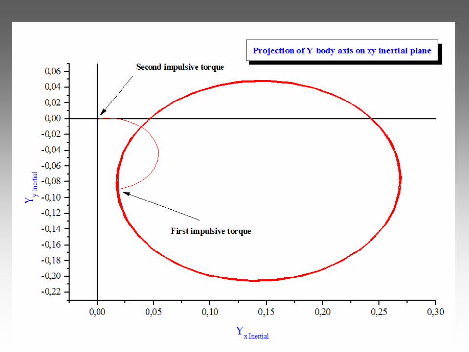
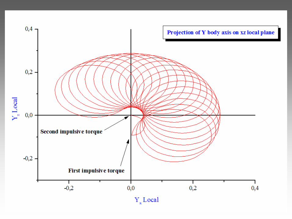
16.2 Precession dumping with two successive impulses (2/3)
Final State
xbody
zbody
-ybody
wheel
xinertial
yinertial
zinertial
L Ixx = 16669.631 Kg m2
Iyy = 2714.554 Kg m2
Izz = 16216.076 Kg m2
Roll = 6o
Pitch = 0o
Yaw = 0o
• Wheel angular momentum : 45 Nms
• Total angular momentum L : 45.3942 Nms
• Precession period : 38.3455 min
• Precession radius : 7.364o
• Angle between angular momentum and z-inertial axis: 9.47o
• Angle between angular momentum and y-body axis: 7.36o
Initial State
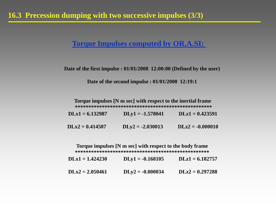
16.3 Precession dumping with two successive impulses (3/3)
Torque Impulses computed by OR.A.SI:
Date of the first impulse : 01/01/2008 12:00:00 (Defined by the user)
Date of the second impulse : 01/01/2008 12:19:1
Torque impulses [N m sec] with respect to the inertial frame
***************************************************
DLx1 = 6.132987 DLy1 = -1.578041 DLz1 = 0.423591
DLx2 = 0.414507 DLy2 = -2.030013 DLz2 = -0.000010
Torque impulses [N m sec] with respect to the body frame
**************************************************
DLx1 = 1.424230 DLy1 = -0.168105 DLz1 = 6.182757
DLx2 = 2.050461 DLy2 = -0.000034 DLz2 = 0.297288

17. Utilization of OR.A.SI for
Actual GEO Orbital
Operations Problem Solving

Utilization as a mission analysis tool.
Validation of the selected inclination control strategy.
Study of the impact that the time distance between inclination and drift/eccentricity
control maneuver execution had on the ergol consumption through the possible increase
of DV for eccentricity control.
Feasibility study of increasing the eccentricity of control in accordance to the various
technological constrains of the spacecraft (maneuver errors), the orbit determination
accuracy and the dimensions of the station keeping window. This was done with the
Longitude Dead Band Breakdown tool.
Determination of the expected number of East-West maneuver couple occurrence for
scheduling maintenance of all branches pertaining to CPS (Combined Propulsion
Subsystem).
Calculation of the optimality of using the long term inclination control strategy proposed
by E.M.Soop in contrast to the utilization of inclination control based on secular drift
correction. Determination of the maximum allowable inclination drift depth.
Validation and simulation of proposed colocation strategies.
Utilization as a propagator for determination of the miss distance with IGSO and HEO
debris which couldn’t be propagated from integrators optimized only for GEO orbits.
Production of orbit data in the form of OEM (CCSDS Standard) and SED (Satellite
Ephemeris Data) for DVB-RCS platforms and ephemeris exchange with other operators.

Utilization for observability analysis.
Determination of the optimal orbit determination setup (selection of antennas and solve
for parameters), corresponding to the maximum attainable orbit determination accuracy
through the calculation of relevant consider covariance error ellipsoid.
Determination of the minimum safe separation for colocation.
Determination of the minimum separation for collision mitigation with space debris.
Tracking and ranging acceptance tests for new TCR antenna. Acquisition of raw range
and angular measurements, development of custom interface for measurement ingestion
from OR.A.SI software, preprocess measurement for noise reduction, orbit
determination and assessment of antenna accuracy based on the consider covariance
analysis of the a posteriori orbit determination error.
Assessment of collision risk with secondary object and calculation of appropriate
collision avoidance maneuver.
Utilization for FAT of new Flight Dynamics software.
Checking the accuracy and stability of the integrator used by the software under test by
comparing its behavior with three different integrators: i) 8th order Runge-Kutta
Dormant-Prince 853 adaptive step size ii) Runge-Kutta Fehlberg RK4(5) adaptive step
size or iii) 8th order Adams-Moulton with fixed step size.
Assessment of celestial events accuracy (IRES Moon and Sun Blindings, eclipse by the
Earth or the Moon, satellite Earth station collinearity).

18. Bibliography Used for
Code Development

Bibliography Used for Code Development (1/4)
1. David A.Vallado, Second Edition 2004. Fundamentals of Astrodynamics and Applications.
2. Oliver Montenburg, Eberhard Gill, First Edition 2000. Satellite Orbits Models, Methods and
Applications.
3. Oliver Montenburg, Thomas Pfleger, Fourth 2002. Astronomy on the Personal Computer.
4. E.M.Soop, 1994. Handbook of Geostationary Orbits.
5. Jean Meeus, Second Edition 1998. Astronomical Algorithms.
6. Peter Duffett-Smith, Third Edition 2003. Practical Astronomy With Your Calculator.
7. Roger R.Bate, Donald D.Mueller, Jerry E.White 1971. Fundamentals of Astrodynamics.
8. William Tyrrel Thomson, Dover Edition 1986. Introduction to Space Dynamics.
9. William E.Wiesel, Second Edition 1997. Spaceflight Dynamics.
10. F.Kenneth Chan, 2008. Spacecraft Collision Probability.
11. U.S. Naval Observatory Washington, D.C – Edited by P.Kenneth Seidelmann, 2006. Explanatory
Supplement to the Astronomical Almanac.
12. Byron D.Tapley, Bob E.Schutz, George H.Born, 2004. Statistical Orbit Determination.
13. Bruce P.Gibbs, 2011. Advanced Kalman Filtering Least-Squares and Modeling.
14. Wilbur L.Pritchard, Henri G.Suyderhoud Robert A.Nelson, Second Edition 1993. Satellite
Communication Systems Engineering.
15. Peter Fortescue, John Stark, Graham Swinerd, Third Edition. Spacecraft Systems Engineering.
16. CNES, Edited by Jean-Pierre Carrou, 1995. Spaceflight Dynamics Part I and II.
17. Haim Baruh, 1999. Analytical Dynamics.
18. Goldstein, Pool & Safco, Third Edition 2002. Classical Mechanics.
19. Athanasios Papoulis, 1990. Probability and Statistics.
20. William H.Press, Saul A.Teukosky, William T.Vetterning, Brian P.Flannery, Second Edition 2005.
Numerical Recipes in C++ The Art of Scientific Computing.

Bibliography Used for Code Development (2/4)
21. Ken Fox, Dept. of Applied Maths., Queen Mary Colledge, London UL, 1984. Numerical
Integration of the Equations of Motion of Celestial Mechanics.
22. L.F. Shampine, Mathematics Department Southern Methodist Univeristy Dallas, 2004. Error
Estimation and Control for ODEs.
23. Matt Berry, Liam Healy, 2003. Comparison of Accuracy Assessment Techniques for Numerical
Integration. Paper AAS 03-171 presented at the 13th AAS/AIAA Space Flight Mechanics Meeting.
24. C.E. Veletz Goddard Space Flight Center. Local-Error Control and its Effects on the Optimization
of Orbital Integration. NASA Technical Note – NASA TN D-4542.
25. Erwin Fehlberg, George C.Marshall Space Flight Center. Classical Fifth-,Sixth-,Seventh-, and
Eight-Order Runge-Kutta Formulas With Stepsize Control. NASA TR R-287.
26. R.A. Broucke, P.I. Cefola, 1971. On the Equinoctial Orbit Elements. Provided by the NASA
Astrophysics Data System.
27. David A.Vallado, 2003. Covariance Transformation for the Satellite Flight Dynamics Operations.
Paper AAS 03-526 presented at the AAS/AIAA Astrodynamics Specialist Conference August 3-7 ,
2003.
28. George Veis. Precise Aspects of Terrestrial and Celestial Reference Frames. SAO Special Report
No.123.
29. George H.Kaplan, 2005.The IAU Resolutions on the Astronomical Reference Systems, Time Scales,
and Earth Rotation Models – Explanation and Implementation. United States Naval Observatory
Circular No.179.
30. CCSDS 502.0-B-2, Blue Book, November 2009. Orbit Data Messages. Recommendation for Space
Data System Standards.
31. CCSDS 508.0-B-1, Blue Book, June 2013. Conjunction Data Message. Recommendation for Space
Data System Standards.
Bibliography Used for Code Development (3/4)
32. Felix R.Hoots, Ronald L.Roehrich, Package Complied by T.S. Kelso, 1988. Spacetrack Report No.3
– Models for Propagation of NORAD Elements Sets.
33. David A.Vallado, Paul Crawford, Richard Hujsak, T.S. Kelso. Revisiting Spacetrack Report #3:
Rev2. AIAA 2006-6753-Rev2.
34. John H.Seago, David A.Vallado, 2000. Coordinate Frames of the U.S. Space Objects Catalogs.
AIAA 2000-4025.
35. P.Wauthier, P.Francken, H.Laroche, 1994. On the Co-location of the Three ASTRA Satellites. Paper
Presented at the International Symposium on the Space Flight Dynamics, St.Petersburg-Moscow ,
May 1994.
36. P.Wauthier, P.Francken, H.Laroche, 1997. Co-location of Six ASTRA Satellites : Assessment After
One Year of Operations.s. Proceedings of the 12th International Symposium on ‘Space Flight
Dynamics’, ESOC, Darmstadt, Germany, 2-6 June 1997.
37. P.Francken, P.Wauthier, 1994. Numerical Simulations of Multiple Satellite Co-location. Paper
Presented at the International Symposium on the Space Flight Dynamics, St.Petersburg-Moscow ,
May 1994.
38. P.Wauthier, P.Francken, 1994. The ASTRA Co-location Strategy for Three to Six Satellites. Paper
Presented at the SCD1 International Symposium on Spacecraft Ground Control and Flight
Dynamics, Sao Jose dos Campos (Brazil), February 1994.
39. M.C. Eckstein, C.K. Rajasingh, P. Blumer, 1989. Colocation Strategy and Collision Avoidance for
the Geostationary Satellites at 19 Degrees West. Paper Presented at the CNES International
Symposium on SPACE DYNAMICS Toulouse (France) 6-10 November 1989.
40. Salvatore Alfano, 2005. Collision Avoidance Maneuver Planning Tool. Paper AAS 05-308 presented
at the 15th AAS/AIAA Astrodynamics Specialist Conference August 7-11 , 2005.
Bibliography Used for Code Development (4/4)
41. Salvatore Alfano, 2005. Relating Position Uncertainty to Maximum Conjunction Probability. The
Journal of the Astronautical Sciences, Vol.53, No.2, April-June 2005, pp.193-205.
42. Salvatore Alfano, 2005. A Numerical Implementation of Spherical Object Collision Probability. The
Journal of the Astronautical Sciences, Vol.53, No.1, January-March 2005, pp.103-109.
43. Salvatore Alfano, 2003. Relating Position Uncertainty to Maximum Conjunction Probability. Paper
AAS 03-548 presented at the AAS/AIAA Astrodynamics Specialist Conference August 3-7, 2003.
44. Felix R.Hoots, Linda L.Crawford and Ronaldo L.Roehrich, 1984. An Analytic Method to Determine
Future Close Approaches Between Satellites. Celestial Mechanics 33 (1984)
45. James Woodburn, Vincent Coppola and Frank Stoner. A Description of Filters for Minimizing the
Time Required for Orbital Conjunction Computations. Paper AAS 09-372.
46. Conrad Schiff. Adapting Covariance Propagation to Account for the Presence of Modeled and
Unmodeled Maneuvers. Paper from AIAA.
47. Saika Aida, Michael Kirschner, Florian Meissner. Collision Risk Assessment and Mitigation Strategy
for the GSOC GEO Satellites.
48. Francois Laporte, 2014. JAC Software, Dedicated to the Analysis of Conjunction Messages. Paper
AIAA 2014-1774 Presented to SpaceOps 2014 Conference 5-9 May 2014 Pasadena, CA.
49. Monique Moury, Lauri K.Newman, Francois Laporte, 2014. Middle Man Concept for In-orbit
Collision Risk Mitigation, CAESAR and CARA Examples. Paper AIAA Presented to SpaceOps 2014
Conference 9 May 2014 Pasadena, CA.
50. Francois Laporte. JAC Software, Software, Solving Conjunction Assessment Issues.
51. Babiker Fathelrahman, Doyon Michel, Abbasi Viqar. The Canadian Space Agency (CSA) Collision
Risk Assessment and Mitigation System (CRAMS): Sharing the Development and the Operational
Challenges.
52. V.Abbasi, M.Doyon, R.Babiker, D.Golla. Advanced Space Situational Awareness through Automated
Conjunction Risk Analysis System (CRAMS).

THANK YOU FOR READING MY PRESENTATIONS