Fleet Management Coordination in Decentralized ...Author: Coordination in Decentralized Humanitarian Operations 3 to the cost of delay than to the eet management cost. The bigger the

Fleet Management Coordination in DecentralizedHumanitarian Operations

We study incentive alignment for the coordination of operations in humanitarian settings. Our research

focuses on transportation, the second largest overhead cost to humanitarian organizations after personnel.

Motivated by field research, we study the fleet size problem from a managerial perspective. In terms of

transportation, an equity focused Humanitarian Program implemented by an International Humanitarian

Organization has private information which affects the balance between equity and efficiency intended by

the Organization’s Headquarters. The incentive alignment issue is complex because traditional instruments

based on financial rewards and penalties are not considered to be viable options. This problem is further

complicated by information asymmetry in the system due to the dispersed geographical location of the

parties. We design a novel mechanism based on an operational lever to coordinate incentives in this setting.

This study contributes to two streams of literature, humanitarian logistics, and incentives in operations

management.

Key words : Incentives, Humanitarian Logistics, Fleet Management

1. Introduction

The need for humanitarian action has increased dramatically in the last few decades and it is

expected to rise significantly in the years to come (Thomas and Kopczak 2005). International

Organizations carrying out humanitarian action face serious challenges to deliver the right goods

and services to the right people at the right time and at the right cost (Van Wassenhove 2006).

Including basic health care provision, nutrition and agriculture, relief and development programs

are the primary channels of humanitarian aid delivery carried out by International Humanitarian

Organizations (IHO). Every year IHO spend more than $1,5 billions running an international fleet

close to 80,000 four wheel drive (4x4) vehicles to support the delivery of humanitarian programs.

Motivated by extensive field research, we study coordination issues in a two-party decentralized

4x4 fleet management system supporting IHO’s programs.

1

Author: Coordination in Decentralized Humanitarian Operations2

Our research is motivated by a larger field project to understand field vehicle fleet management

in IHO. The field project includes three large IHO using global procurement managed at the Head-

quarters level: the International Committee of the Red Cross (ICRC), the International Federation

of Red Cross and Red Crescent Societies (IFRC), and the World Food Programme (WFP). Staff

interviews with various IHO were conducted at the Headquarters in Europe and the Middle East,

as well as at national and field program levels in the Middle East and Africa. In the following we

will briefly describe the research problem and use our findings from the field research to motivate

the theoretical model that is studied in this paper.

The fleet management system has two decision-making parties: the Program and the Head-

quarters. Often located in remote areas of developing countries (the field), Programs are service

oriented. They provide assistance and help alleviating the suffering of people in the aftermath of

disasters (relief). Also, Programs implement activities to improve the quality of life of poor commu-

nities (development). Transportation requirements for relief and development are different. Relief

Programs assign vehicles according to emergency priorities for disaster assessment, or to coordi-

nate search, rescue and emergency aid distribution operations. Development Programs use vehicles

for regular visits to villages or refugee camps for health care or to coordinate aid distribution.

Urgency in development Programs is lower and vehicles are typically assigned to visits in order of

requisition. We focus on fleet management in development Programs with big fleets of twenty or

more vehicles in the same geographic location. Development Programs are henceforth referred to

as Programs.

Some examples of Programs include health, nutrition, water and sanitation. In terms of trans-

portation, the objective of Programs is to have a vehicle available when it is required by their staff

to visit beneficiaries. Although speed in demand fulfillment is not necessarily critical, Programs

must meet demand in a reasonable time. Due to the long-term nature of Programs, visits that

cannot be performed on time are accumulated. The Program incurs two main costs, the cost of

delay and the cost of managing their fleets in the field. Often Program managers are more sensitive


to the cost of delay than to the fleet management cost. The bigger the fleet the lower the cost of

delay. During the planning stage, the Program states its transportation needs to the Headquarters.

The Headquarters have the function of procuring the fleet requested by the Program. Typically

located in the US or Europe, the Headquarters’ objective is balancing the cost of delay of last mile

distribution and the operating cost of the fleet, i.e. the fleet management cost plus the running

cost. During the planning stage, the Headquarters decide the optimal fleet size to minimize the

system’s cost. The fleet size includes a fleet buffer to guarantee that a reasonable proportion of

visits will not suffer any delay. The fleet buffer determines the service level of the fleet. The bigger

the fleet buffer the lower the cost of delay but the higher the operating cost of the fleet.

In summary, the Program states its transportation needs to the Headquarters and manages the

fleet in the field. The Headquarters assign operational capacity (fleet) to the Program. Program‘s

transportation needs are stochastic and private information. Both the Headquarters and the Pro-

gram incur a disutility due to the delay in reaching IHO’s beneficiaries. But only the Headquarters

are accountable for the full operating cost of the fleet. Since the operating cost increases with the

fleet size, the Headquarters optimal fleet size is smaller than the calculated by the Program. Hence,

the Program may have incentives to distort its needs to get a larger fleet. Due to particular charac-

teristics of humanitarian operations related to earmarked funding, transferring the accountability

of the full operating cost to the Program is not feasible. Additionally, standard financial-incentives-

based mechanisms are not considered viable in this humanitarian setting. This is primarily due

to the organizational culture of the IHO, wherein the employees are driven by their motivation to

serve and not by the objectives such as profit maximization (Lindberg 2001, Manell 2010). E.g., it

is almost inconceivable for the IHO to incentivize volunteer medical doctors working in the field

by using financial penalties and rewards.

The Headquarters monitor the Program’s stated needs but unfortunately it does not deter pro-

grams from needs distortion. The incentives problem is illustrated by quotes from our interviews.

One of the Headquarters staff said:

“I feel some of our programs have more vehicles than required”


In fact, one of the Senior Fleet Managers we interviewed in Geneva, Switzerland estimates that

their Programs have between 10% and 15% more vehicles than required. In contrast, when we

asked about the fulfillment of his transportation needs, a development Program manager in the

Zambezia Province, Northern Mozambique said:

“Often we have to wait too long to have a vehicle available to go to the field”

These quotes refer to the steady state behavior of the system instead of referring to the punctual

– and expected – mismatches between stochastic demand and stochastic supply. In fact, to respond

to a stochastic demand, the fleet management system uses the fleet buffer, which is decided by

calculating a buffer factor that should balance the service level and the operating cost of the

fleet. Combining mechanism design and heavy traffic queueing theory we develop a non-trivial but

tractable model to coordinate incentives in this setting. We use the buffer factor to induce truth

revelation from the Program. Our model provides insights to overcome current inefficiencies in

decentralized humanitarian systems. In some instances our model is able to reduce the fleet excess

in more than 10%, matching the intuition of senior fleet managers. We also obtain counterintuitive

results regarding the value of private information in a decentralized humanitarian system.

We believe that the unique characteristics of IHO make the incentive misalignment issues an

extremely interesting research topic, and not just a mere application of the principal-agent frame-

work from the economics literature. Our work should appeal to the Operations Management com-

munity as it showcases the strategic importance of operational design beyond the objective to

achieve tactical efficiency in the humanitarian sector. The model can be used to advance the aca-

demic understanding of decentralized decision-making in humanitarian operations. To the best of

our knowledge, this is the first analytical study of decentralized humanitarian operations completely

informed by field research.

2. Literature Review

This paper contributes to the humanitarian logistics literature and to the incentives literature

in operations management. There is an increasing interest in studying humanitarian operations


(Altay and Green 2006). Extant literature on humanitarian logistics follows a classical optimization

approach. Most of the research examines stochastic relief systems for disaster preparedness or for

disaster response. Typically, the literature applies operations research techniques to relief settings

assuming central planner coordination. The objective can be equity or cost-efficiency oriented.

Equity-based objective functions have been studied in terms of time of response and demand

fulfilment. Research to minimize the time of response can be found in Chiu and Zheng (2007) and

Campbell et al (2008). Research exploring demand coverage include Batta and Mannur (1990),

Ozdamar et al (2004), Jia et al (2007), De Angelis et al (2007), Yi and Ozdamar (2007),

Saadatseresht et al (2009), and Salmeron and Apte (2010).

Cost-based objective functions are often represented either via monetary cost or via travel dis-

tance. Cost minimization can be found in the work of Barbarosoglu et al (2002), Barbarosoglu and

Arda (2004), Beamon and Kotleba (2006) and Sheu (2007). Distance traveled minimization has

been explored by Cova and Johnson (2003), Chang et al (2007), and Stepanov and Smith (2009).

In their work, Stepanov and Smith also examine an equity based function of time of response.

Regnier (2008) models the trade-off between cost and equity in hurricane evacuation operations,

also from a central planner perspective. In contrast to extant literature in humanitarian logistics

we analyze incentives in a decentralized system.

The incentives literature on adverse selection discusses settings where there are agents of different

type. Agents know their types while the principal does not (Green and Laffont 1977, Dasgupta et al

1979, Myerson, 1979, Harris and Townsend 1981, Maskin and Riley 1984). When offered a menu of

contracts of particular characteristics, these agents reveal their type following the revelation princi-

ple. The supply chain management literature on incentives has focused on exploring manufacturing

and service operations management in “for profit” settings. Typically, decisions in manufactur-

ing supply chains relate to order-quantity of goods while decisions in service supply chains relate

to the capacity of the service system. Most of the mechanisms for supply chain coordination in

manufacturing and in service operations management are based on financial incentives.


In this paragraph we briefly summarize some commonly studied financial contracts in manufac-

turing and service supply chains. This is not a comprehensive list of the vast literature on supply

chain contracts, but it provides the readers a primer on the nature of contracts that have been

studied in such settings. In revenue sharing contracts a retailer pays a supplier a wholesale price

for each unit purchased plus a percentage of the revenue generated by the retailer (Cachon and

Lariviere 2005). Buy-back contracts have a wholesale price and a buy-back price for unsold goods

(Pasternack 1985). In Sales-rebates contracts the supplier charges the retailer a per-unit wholesale

price but gives the retailer a rebate per unit of goods sold above a predefined threshold (Krishnan

et al 2001, Taylor 2002). In quantity discount contracts the retailer receives a discount either

on all units if the purchased quantity exceeds a threshold (all-unit quantity discount) or on every

additional unit above a threshold (incremental quantity discount) (Corbett and de Groote 2000,

Cachon and Terwiesch 2009). In price-discount contracts wholesale prices are discounted on the

basis of annual sales (Bernstein and Federgruen 2003). Our research departs from this stream of

literature since we use a non-financial, capacity-based mechanism for system coordination.

In service systems decisions are based on capacity. For instance, Hasija et al (2008) explore

pay-per-call and pay-per-time contracts in call-centers. In the first type of contracts the vendor

earns a fixed fee from the client for each served phone call. In the second type of contracts the

vendor is paid per unit of time spent serving customers. In this service setting as in the previ-

ous manufacturing ones coordination is achieved via financial transfer payments. Departing from

financial mechanisms, Su and Zenios (2006) explore the efficiency-equity trade-off in kidney trans-

plantation. In their setting financial transfers are not possible. They propose a kidney’s allocation

rule based on the fact that lower-risk patients are willing to spend more time waiting in order to

receive organs of higher quality. Instead of an allocation rule we propose a capacity (fleet buffer)

rule for fleet coordination. Our contribution is twofold. First, we develop the first analytical model

of decentralized humanitarian operations completely informed by field research. Second, using a

combination of heavy traffic models with mechanism design we develop a mathematically tractable


model using operational levers that respect exogenous constraints that exist in the humanitarian

context.

3. The Fleet Management System

The system is composed by two parties: the Headquarters and the Program. Based on system cost

considerations, the Headquarters decide a service level for the fleet and procure the vehicles from

a global source. The Headquarters are also in charge of monitoring the Program’s transportation

needs whenever it is required.

The Headquarters are accountable for the total cost of the system. The total cost includes

the running cost of the fleet, the fleet management cost in the field, and the cost of delay. The

running cost of the fleet, r, is the average running cost per vehicle per unit of time. It includes

maintenance, repairs, and fuel costs (Pedraza-Martinez and Van Wassenhove 2010). The running

cost is an overhead cost to the IHO. The fleet management cost, c, is the average management cost

per vehicle per unit of time. Pedraza-Martinez et al (2011) find that the Program is accountable

for c. During our field visits we observed that senior humanitarian staff in the field often dedicate

a proportion of their time to fleet scheduling and routing. The fleet management cost also includes

the cost of vehicle drivers, which are instrumental to Program delivery due to their knowledge of

local language and geography. Finally, the fleet management cost includes the cost of information

systems and spreadsheets to track fleet scheduling and routing in the field. The field management

cost in the field is a direct cost to the Program. We refer to c+ r as the operating cost of the fleet.

The cost of delay, w, is measured per field visit per unit of time. The Program incurs the cost

of delay and it is accountable for it. Although the cost of delay is not a cash cost to the Program,

it results in a disutility associated with delay in carrying out Program delivery. To simplify our

analysis and capture both the disutility of delay and the tensions of this decentralized system we

assume a constant marginal cost.

The Program reports its transportation needs to the Headquarters and uses the fleet to coordi-

nate and execute last mile distribution. The Program uses the fleet for transportation of staff to


visit beneficiaries, transport of materials, and transport of items for distribution to beneficiaries

(Pedraza-Martinez et al 2011). Although demand is more stable through time than in relief set-

tings, humanitarian development work has some stochasticity – in both arrivals and service times.

This comes from the mobility of beneficiaries and the unpredictability of operating conditions in

terms of weather, road conditions and security. In case of unavailability of vehicles to carry out the

visits to beneficiaries the demand tends to accumulate but it rarely disappears.

To capture the stochasticity of the system and the nature of work accumulation when the Pro-

gram faces a fleet shortage, we use a queueing model. The use of queueing models for vehicle fleet

management systems is well established in the literature. Queueing models have been used for

analyzing police patrol systems (Green 1984, Green and Kolesar 1984a, 1984b, 1989, 2004), fire

departments (Kolesar and Blum 1973, Ignall et al 1982), helicopter fire fleets (Bookbinder and

Martell 1979), and ambulance fleets (Singer and Donoso 2008). These papers model transportation

needs using stochastic inter-arrival times.

We represent the Program’s transportation needs with the Greek letter λ. The transportation

needs are measured in rate of visits per unit of time. Service times, µ, are also stochastic. For

simplicity, we assume µ = 1, which corresponds to measuring time in the scale of mean service

times (Whitt 1992).

To balance the system costs, i.e. the operating cost and the cost of delay, the Headquarters decide

on the fleet size. In a deterministic setting the minimum fleet size for the system would be λ/µ.

However, a fleet buffer is required to maintain stability of the system due to inherent variability

in inter-arrival and service times. In other words, the fleet buffer is the extra-number of vehicles

needed for protecting the system from stochasticity and achieving a predetermined service level.

We model the system as an Erlang-C system following a first-come first-served queueing disci-

pline. This rule was chosen since, as mentioned before, within the Program all the visits have the

same priority. For analytical tractability we use heavy-traffic approximations under the “rational-

ized regime” to represent the average delay in the system. The Halfin-Whitt (1981) delay function,


π(y) is an asymptotically exact approximation to the probability of delay, Pr{wait> 0}. The value

of π(y) is:

π(y) =

[1 +

yΦ(y)

φ(y)

]−1Φ(y) and φ(y) are the unit normal cdf and pdf, respectively. The service level of the fleet is the

average proportion of visits carried out without delay. The Program that is assumed in our system

neither carries out emergency response activities nor highly scheduled regular work, but carries

out delay sensitive and stochastically arriving developmental activities. Therefore we believe that

the rationalized regime is appropriate for this setting.

Borst et al (2004) show that a square-root staffing rule is asymptotically optimal for a system

operating in the rationalized regime. Following Halfin and Whitt (1981), Grassman (1988), Whitt

(1992), Borst et al (2004), Hasija et al (2005) we use the square-root staffing rule

F (γ) = λ+ γ(c, r,w)√λ (1)

to calculate the fleet size. Denoted by γ, the buffer factor is the key decision variable to determine

the fleet buffer. The optimal buffer factor can be obtained via optimization methods by balancing

the importance of delays in visits with fleet operating costs.

The effectiveness of the square-root rule increases in the size of the fleet and it has been shown

that it is a robust approximation for the optimal system size of fleets of 20 or more vehicles.

According to Borst et al (2004) and Hasija et al (2005), for a given buffer factor γ the average

number of visits in the queue is Q(γ) = π(γ)λ

Fµ−λ . Using µ= 1 and replacing F by its definition in (1)

we obtain:

Q(γ) =π(γ)√λ

γ(2)

3.1. Centralized Benchmark

In a centralized system the central planner minimizes the total system cost given by the average

cost of delay wQ(γ) plus the average operating cost of the fleet (c+ r)F (γ). The central planner’s

problem is:


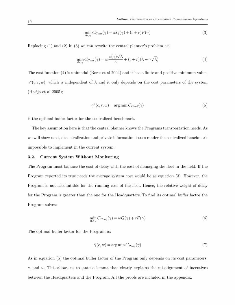
min0<γ

CCent(γ) =wQ(γ) + (c+ r)F (γ) (3)

Replacing (1) and (2) in (3) we can rewrite the central planner’s problem as:

min0<γ

CCent(γ) =wπ(γ)√λ

γ+ (c+ r)(λ+ γ

√λ) (4)

The cost function (4) is unimodal (Borst et al 2004) and it has a finite and positive minimum value,

γ∗(c, r,w), which is independent of λ and it only depends on the cost parameters of the system

(Hasija et al 2005);

γ∗(c, r,w) = arg minCCent(γ) (5)

is the optimal buffer factor for the centralized benchmark.

The key assumption here is that the central planner knows the Programs transportation needs. As

we will show next, decentralization and private information issues render the centralized benchmark

impossible to implement in the current system.

3.2. Current System Without Monitoring

The Program must balance the cost of delay with the cost of managing the fleet in the field. If the

Program reported its true needs the average system cost would be as equation (3). However, the

Program is not accountable for the running cost of the fleet. Hence, the relative weight of delay

for the Program is greater than the one for the Headquarters. To find its optimal buffer factor the

Program solves:

min0<γ

CProg(γ) =wQ(γ) + cF (γ) (6)

The optimal buffer factor for the Program is:

γ̄(c,w) = arg minCProg(γ) (7)

As in equation (5) the optimal buffer factor of the Program only depends on its cost parameters,

c, and w. This allows us to state a lemma that clearly explains the misalignment of incentives

between the Headquarters and the Program. All the proofs are included in the appendix.


Lemma 1. γ∗(c, r,w)< γ̄(c,w).

Equation (1) together with lemma 1 imply that the optimal fleet size for the Headquarters is

smaller than the optimal fleet size for the Program. In other words, both the Headquarters and

the Program consider the full cost of delay, but the Program considers only a portion of the

operating cost, which the Headquarters fully internalize. Since the operating cost increases with

the fleet size, then the Headquarters optimal fleet size will be smaller than the one calculated by

the Program. This result is consistent with our field observations, in particular with the worries of

the Headquarters in terms of oversized fleets. The result is also consistent with the worries of the

Program in terms of not having enough vehicles to optimize their service.

The true transportation needs are private information to the Program. The misaligned incentives

and private information create an adverse selection issue, and the Program may distort its stated

transportation needs. We abstract the Program to two types: low transportation needs, L, and

high transportation needs, H, and λL < λH . This standard assumption helps us to capture the

main trade-offs of equity and efficiency while keeping the model analytically tractable. In reality,

we observed that λH is easy to estimate since the maximum number of vehicles is determined by

the total number of humanitarian staff in the Program. For instance, in a Program with 25 medical

doctors, the IHO would not procure more than 25 vehicles. Nevertheless, possible coordination in

fleet scheduling could results in a decrease in transportation needs, leading to λL. By stating its

transportation needs, λ̂i, the i∈ {L,H} type program would target an intended buffer factor δ(λ̂i)

such that

δ(λ̂i) =λ̂i + γ

√λ̂i−λi√λi

(8)

From (8) follows that δ(λ̂i) |λ̂i=λi= γ. Let

δL = δ(λ̂L) |λ̂L=λH, and δH = δ(λ̂H) |λ̂H=λL

(9)


Note that δL >γ and δH <γ follow from the fact that λL <λH . For a given i type Program the

current system’s cost would be:

CCurr(δ(λ̂i)) =wQi(δ(λ̂i)) + (c+ r)Fi(δ(λ̂i)) (10)

Also note that for γ = γ∗ in (8) we have CCent(γ∗)<CCurr(δi).

A straightforward way to coordinate the system would be by transferring the accountability of

running costs of the fleet to the Program. The running costs are an overhead and the Headquarters,

which are considered a support function, are accountable for these costs. Due to accountability

reasons particular to the humanitarian sector the internal transfer of running cost’s accountability

is not possible. Aware of the potential increase in cost coming from transportation needs distortion

but unable to transfer the entire cost to the Program, the Headquarters react to transportation

needs distortion by monitoring the Program’s stated needs.

3.3. Current System With Monitoring

The Headquarters don’t know the Program’s true transportation needs, but they have some idea

–just not a very accurate one. So we assume that the Headquarters have a probabilistic prior belief

that:

λi =

{λL, w.p. q

λH , w.p. 1− q

The Headquarters can monitor λ̂i before procuring the fleet. To monitor, the Headquarters have

to carefully check the Program’s data records. During our field visits we observed that Programs

often have detailed data on fleet use and transportation needs in the field. Typically the data is in

printed form, ready for auditing purposes but it is not stored in a way that can be easily accessed

by the Headquarters. Due to the lack of trustworthy information systems on transportation needs

at the national level, the Headquarters may send staff to the field to monitor the Program’s esti-

mated workload in situ. The Headquarters exert a monitoring effort p∈ [0,1] corresponding to the

proportion of Programs to monitor. The monitoring cost is m(p), a function of the monitoring


effort. By sending staff to the field, the Headquarters can get an accurate estimation of the Pro-

gram’s transportation needs. We assume that by monitoring the Headquarters can know the true

transportation needs of the Program. Hence the Program’s problem becomes:

minλ̂i∈{L,H}

Ep[CProg(δ(λ̂i))] = p (wQi(γ) + cFi(γ)) + (1− p)(wQi(δ(λ̂i)) + cFi(δ(λ̂i))

)(11)

The first thing to note is that in the current system the high type Program always reveals its true

transportation needs. This is formalized in the following proposition.

Proposition 1. In the current system CProg(γ∗)<Ep[CProg(δH)]

The intuition behind Proposition 1 comes from the fact that the intended buffer factor from

distortion of transportation needs for the high type Program is lower than the buffer factor offered

by the Headquarters. Additionally, the buffer factor offered by the Headquarters is lower than

the optimal fleet buffer for the Program (Lemma 1). Since the cost function for the Program is

unimodal with minimum in γ̄ (equation 7), it is always cheaper for the high type Program to reveal

the truth. Otherwise, the extra-cost of delay would overcome the savings on fleet management.

We are left with the low type Program. The low type Program states its true transportation

needs as long as CProg(γ∗)<CProg(δL). This suggests the existence of a threshold for truth telling,

formalized in the following proposition.

Proposition 2. For any given values of λL and λH there exists a truth telling threshold γ̂L such

that γ̂L 6= γ∗ and:

if γ < γ̂, then CProg(γ)>Ep[CProg(δL)],

if γ > γ̂, then CProg(γ)<Ep[CProg(δL)]

The threshold value satisfies: Ep[CProg(δL)] =CProg(γ∗)

Since δL also depends on γ∗, λL and λH , for a fixed value of γ∗ the truth telling threshold depends

on the ratio between λH and λL. The threshold indicates that if the ratio λH/λL is big enough, the


low type Program’s savings in cost of delay are overcome by the extra-cost of fleet management. In

summary, the Headquarters know that the high type Program will not distort its needs and the low

type Program will only distort its needs for values of γ < γ̂L. Hence, the Headquarters monitoring

effort should only focus on those Programs reporting high type.

Note, however, that there is no penalty for distortion, i.e. the Program’s stated transportation

needs are independent of the Headquarters monitoring effort. This result is formalized in the

following proposition.

Proposition 3. The Headquarters monitoring effort does not have an influence on whether the

Program truly reveal its type

The lack of effectiveness of monitoring comes from the fact that there is no cost for the Program

from being caught distorting its needs. Given the humanitarian nature of Program delivery it is

not feasible for the Headquarters to impose a penalty to the Program. The Headquarters choose a

monitoring effort solving the following problem:

minp

CMon(γ, δi(λ̂i)) = p[q(wQL(γ) + (c+ r)FL(γ)) + (1− q)(wQH(γ) + (c+ r)FH(γ))] (12)

+ (1− p)[q(wQL(δ(λ̂L)) + (c+ r)FL(δ(λ̂L)) + (1− q)(wQH(δ(λ̂H)) + (c+ r)FH(δ(λ̂H))] +m(p)

The results of propositions 1 and 2 allow us to solve the monitoring problem using backward

induction:

P =

{min{m′−1(q[(c+ r)[FL(δL)−FL(γ)]−w[QL(γ)−QL(δL)]]),1}, if λ̂L = λH

0, otherwise(13)

In the next section we will explore a different, capacity-based mechanism to induce truth reve-

lation from the Program.

4. Operational Mechanism

Since financial transfer payments are not implementable in this setting, truth revelation proves to

be challenging. In this section we propose a novel mechanism design for truth revelation based on

an operational lever, the buffer factor offered by the Headquarters.


The Headquarters (Principal) allocate the Program type i (Agent) an outcome F , i.e. a fleet

size, as a function of the reported type. This is operationalized by the Headquarters committing

to an offered buffer factor, γi, for the stated transportation need of the Program equal to λ̂i. The

Program reports a type profile λ̂i and the mechanism is executed. The Headquarters’ objective is

to minimize the system cost for a given distribution of Program types. The incentive compatibility

(IC) constraints consist of offering each Program type i= {L,H} a buffer factor γi to guarantee

that CProg(γi)≤CProg(δi).

During our field visits we observed that Programs do not have an outside option since the

Headquarters procure the fleet. Hence, the individual rationality (IR) constraints are defined by

the fact that the Headquarters must offer each Program type a buffer factor big enough to protect

the system from stochasticity, i.e. 0<γi. The mechanism is formulated as:

min0<γL,0<γH

E[CMec(γL, γH)] = q [wQ(γL) + (c+ r)F (γL)] + (1− q) [wQ(γH) + (c+ r)F (γH)]

S.T. (14)

(ICL) : wQ(γL) + cF (γL)≤wQ(δL) + cF (δL)

(ICH) : wQ(γH) + cF (γH)≤wQ(δH) + cFδH)

The left hand side of IC constraints in expression (14) is the i type Program cost with a fleet buffer

γi. The right hand side of IC constraints in (14) represents the cost of the i type Program when

distorting its needs. The intended fleet buffer δi is defined by (9).

We now show that there exist fleet buffers γL and γH such that both Program types have

incentives to reveal their true transportation needs. We consider the case of both IC constraints

loose, one IC constraint active, and both IC constraint active.

Let

γ̃L = {γ 6= γL :CProg(γ) =CProg(γL)} (15)

There exist two ways of making the low type Program’s IC constraint tight. The first way is

by forcing γL = δL. The second way of making the low type Program’s IC constraint tight is by

choosing γH such that δL = γ̃L.


Proposition 4. There exist two regions for induced truth revelation via the operational mech-

anism as follows:

1) R1: Equal fleet size region. γH <γ∗ <γL such that F (γL) = F (γH)

2) R2: Different fleet size region. γ∗ < γL, γ∗ < γH such that F (γL) < (γH) and the regions for

induced truth telling are separated by the threshold T1.

The two regions characterized by Proposition 4 can be depicted in the space defined by the trans-

portation needs ratio and probability types (figure 1). In R1 of Proposition 4 both IC constraints

in mechanism (14) are binding. The Headquarters offer δH = γH < γ∗ < γL = γL such that both

Program types receive the same fleet size, F (γL) = F (γH)). This region exists for values of λH/λL

close to 1 and limited by T1, a threshold implicitly defined by the cost parameters of the system,

c, r and w, the lambda ratio, λH/λL and the low type probability, q. When parameters fall in R1,

truth revelation is achieved by making the low type Program indifferent between reporting its true

needs and distorting these needs, i.e. by making the low type IC constraint tight via γL = δL. The

extra-cost for low type’s truth revelation is mitigated by reducing δL via the decrease of γH , such

that γH = δH . In our numerical experiments we show that the cost mitigation is mediated by q, the

low type probability. Increasing q after the threshold T1 reduces the width of R1. Because γH = δH ,

in R1 the high type Program is indifferent between revealing its true transportation needs and

distorting.

In R2 of Proposition 4 only the IC constraint for the low type Program in (14) is binding.

Both γL and γH are greater than γ∗, which means that the Headquarters give incentives to both

Program types. For low values of q the Headquarters keep γH closer to γ∗ by making γ∗ <γH <γL,

due to the likelihood of having a larger proportion of high type Programs. By splitting the buffer

factor, the Headquarters avoid a big increase in the high type Program cost while making the low

type Program IC constraint tight, via δL = γ̃L. For large values of q the increase in the likelihood

of having low type Programs switches the order of incentives to γ∗ < γL < γH . The closer γL is to

γ∗ the lower the cost for the system. As mentioned earlier, we find that as q increases, the region


R2 becomes more favorable than the region R1. The intuition is as follows. In R2, F (γL)<F (γH)

while in R1, F (γL) = F (γH). As q increases, the probability of a Program to be of the low type

increases. Hence F (γL) < F (γH) becomes a more cost effective mechanism than F (γL) = F (γH).

In R2 also characterized in Proposition 4 the high type Program is better of by revealing its true

transportation needs since condition δH <γH < γ̄ implies CProg(γH)<CProg(δH).

With both constraints loose, neither of the Program types has incentives to distort their trans-

portation needs, i.e. there exists a natural truth telling region. Natural truth revelation follows

directly from Proposition 2. The result is formalized in the following corollary.

Corollary 1. There exists a “natural truth telling” region for the operational mechanism. R3,

the natural truth telling region is defined by γ∗ = γL = γH such that FL <FH .

Truth revelation In R3, characterized by corollary 1, is achieved without the need of incentives.

With parameter values falling in this region the low type Program does not have incentives for

distorting its needs. If the low type Program distorts its transportation needs, then it gets a fleet

big enough to guarantee that the cost of management will overcome the savings in delay. On the

other hand, the high type Program does not distort its needs because it would receive a fleet too

small for its needs. In this case the cost of delay would overcome the savings in fleet management.

It is interesting that T2 is independent of q. It depends on the cost parameters c, r, w, and the

λH/λL ratio.

∈(0,1) FL = FH

γH < γ∗< γL γ∗< γL ,

FL <

R1: R2:

λH/

q∈(0,1)

γ L

T1

γ∗< γH γ∗ = γL = γH

< FH

R2: R3:

FL < FH

/λL

γ γH γ γL γH

Natural Truth

Revelation

T2

Figure 1 Truth telling regions in the transportation needs ratio and probability type (γH/γL, q) space


To summarize, by being flexible in choosing fleet buffers γL and γH instead of a unique γ∗, the

Headquarters can create operational incentives for truth revelation. There are two ways of achieving

truth revelation via the operational mechanism: induced and natural. In the case of induced truth

revelation we find that the IC constraint of the low type Program will always be binding. These

incentives potentially increase the system’s efficiency without the need of monitoring the Program’s

reported needs. The operational mechanism has the counterintuitive characteristics that the greater

the different between types the lower the value of private information for the low type program.

The lost of value of information for the low type Program as well as the cost savings for the system

in the different models are explored further in the next section.

5. Numerical Study

This section presents a numerical study that complements the analytical insights presented in

the previous section. The base case uses weekly planning for a time horizon of 52 weeks. The

running cost and the fleet management cost of the fleet are calculated following the research by

Pedraza-Martinez and Van Wassenhove (2010) on vehicle replacement in a humanitarian setting.

The running cost per vehicle is established at $17,000 per year. This is equivalent to $269,23 per

week. It includes maintenance, repairs and fuel. The fleet management cost is set to be 15% of

the running cost. It includes the time of staff coordinating fleet management, and the salary of

vehicle drivers, which depend on the Program (Pedraza-Martinez et al 2011). The normalized

demand rate for the low type Program is λL = 60 visits per week. This is equivalent to a fleet

of 60 vehicles with a utilization of 100%. We assume that the monitoring cost equals the fleet

management cost. In the numerical examples we use a convex monitoring cost function m(p) =

m[qF (γ,λL) + (1 − q)F (γ,λH)]p2. This signifies that the monitoring cost is proportional to the

expected fleet size. We compare the cost of: 1) centralized benchmark; 2) current system without

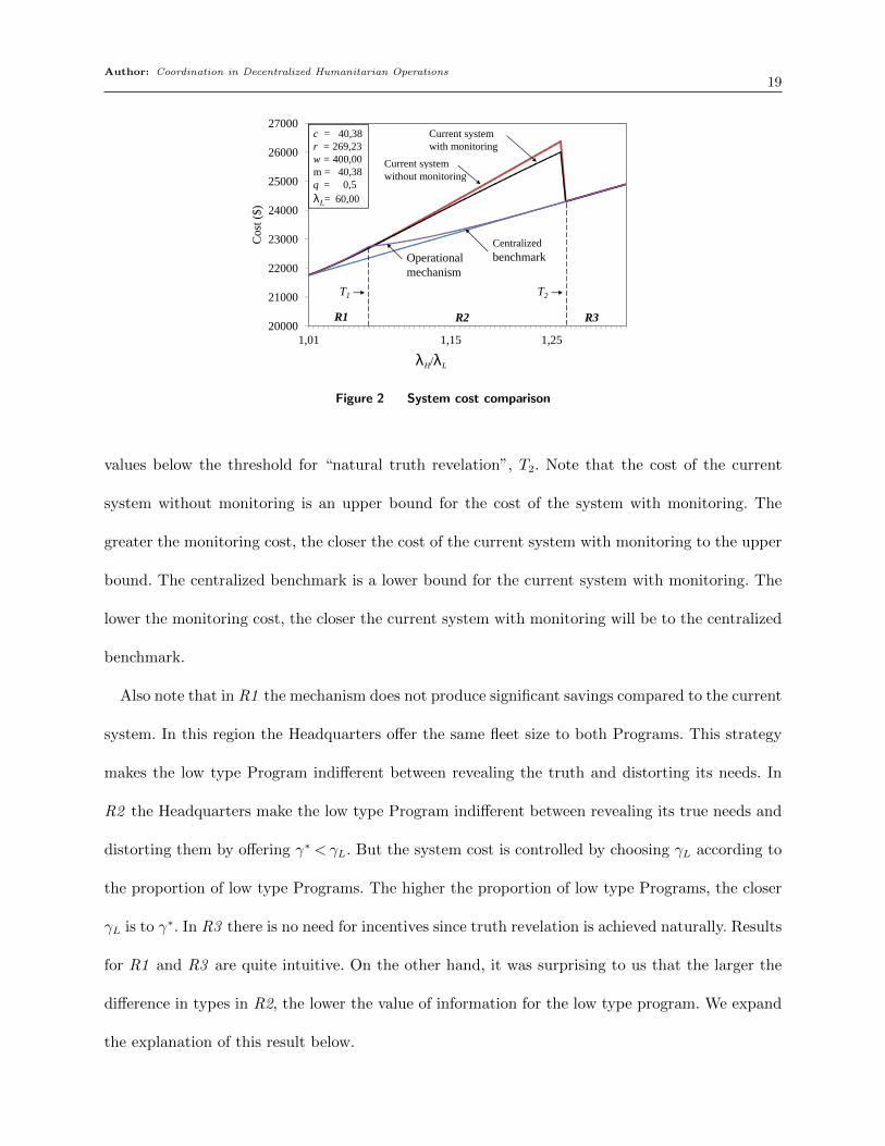
monitoring; 3) current system with monitoring; 4) operational mechanism (figure 2 ).

The cost of the current system without monitoring suffers from a fleet excess caused by the infla-

tion of transportation needs coming from the low type Program. This inflation holds for parameter


23000

24000

25000

26000

27000

Cos

t ($)

Current system with

Current system without monitoring

c = 40,38r = 269,23w = 400,00m = 40,38q = 0,5λL= 60,00

20000

21000

22000

23000

1,01

1,01

51,

021,

025

1,03

1,03

51,

041,

045

1,05

1,05

51,

061,

065

1,07

1,07

51,

081,

085

1,09

1,09

51,

11,

105

1,11

1,11

51,

121,

125

1,13

1,13

51,

141,

145

Cos

t ($)

λH/λL

Operationalmechanism

T1

R1

1,01 1,15

Centralized

Current system with monitoring

Current system monitoring

1,14

1,14

51,

151,

155

1,16

1,16

51,

171,

175

1,18

1,18

51,

191,

195

1,2

1,20

51,

211,

215

1,22

1,22

51,

231,

235

1,24

1,24

51,

251,

255

1,26

1,26

51,

271,

275

1,28

1,28

51,

291,

295

1,3

1,30

51,

311,

315

1,32

1,32

5

L

CentralizedbenchmarkOperational

mechanism

T2

R2 R3

1,15 1,25

Figure 2 System cost comparison

values below the threshold for “natural truth revelation”, T2. Note that the cost of the current

system without monitoring is an upper bound for the cost of the system with monitoring. The

greater the monitoring cost, the closer the cost of the current system with monitoring to the upper

bound. The centralized benchmark is a lower bound for the current system with monitoring. The

lower the monitoring cost, the closer the current system with monitoring will be to the centralized

benchmark.

Also note that in R1 the mechanism does not produce significant savings compared to the current

system. In this region the Headquarters offer the same fleet size to both Programs. This strategy

makes the low type Program indifferent between revealing the truth and distorting its needs. In

R2 the Headquarters make the low type Program indifferent between revealing its true needs and

distorting them by offering γ∗ <γL. But the system cost is controlled by choosing γL according to

the proportion of low type Programs. The higher the proportion of low type Programs, the closer

γL is to γ∗. In R3 there is no need for incentives since truth revelation is achieved naturally. Results

for R1 and R3 are quite intuitive. On the other hand, it was surprising to us that the larger the

difference in types in R2, the lower the value of information for the low type program. We expand

the explanation of this result below.


5.1. Lost of Value of Private Information for the Low Type Program

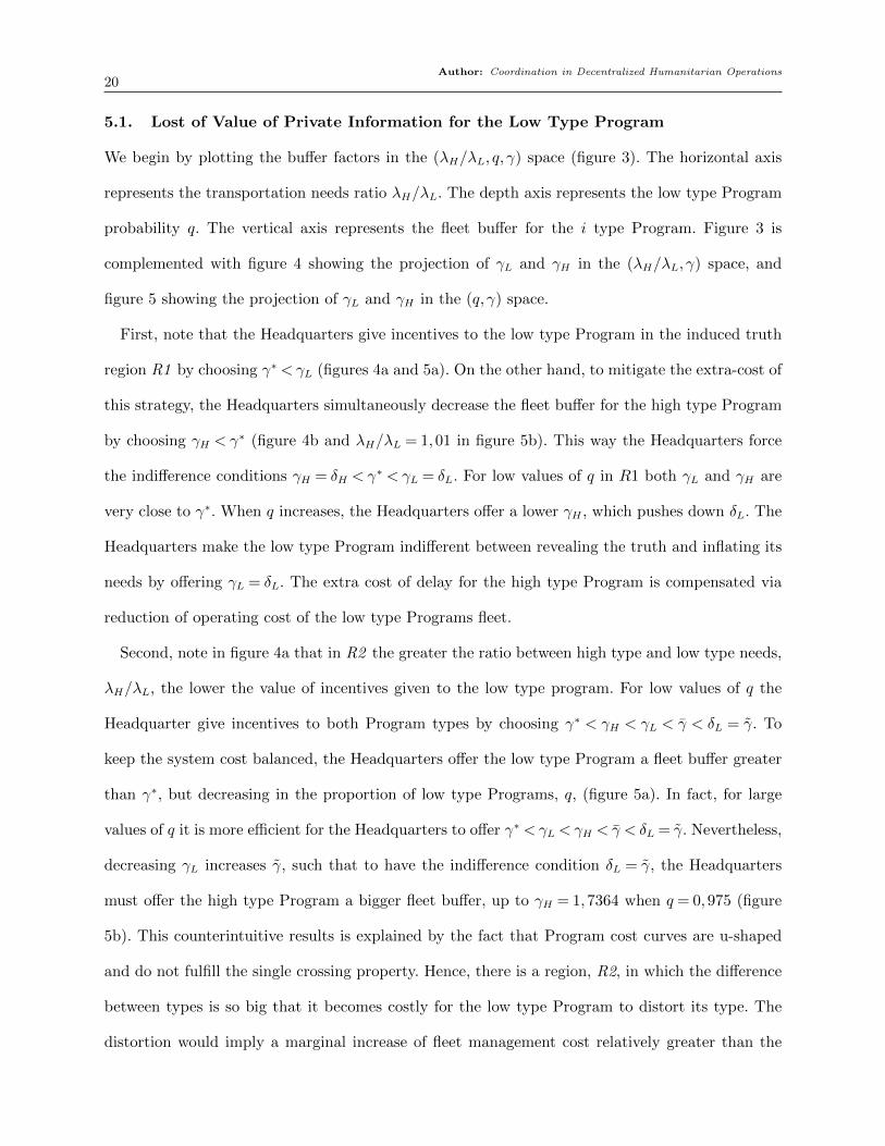
We begin by plotting the buffer factors in the (λH/λL, q, γ) space (figure 3). The horizontal axis

represents the transportation needs ratio λH/λL. The depth axis represents the low type Program

probability q. The vertical axis represents the fleet buffer for the i type Program. Figure 3 is

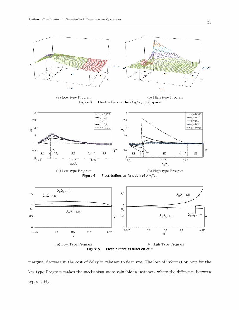
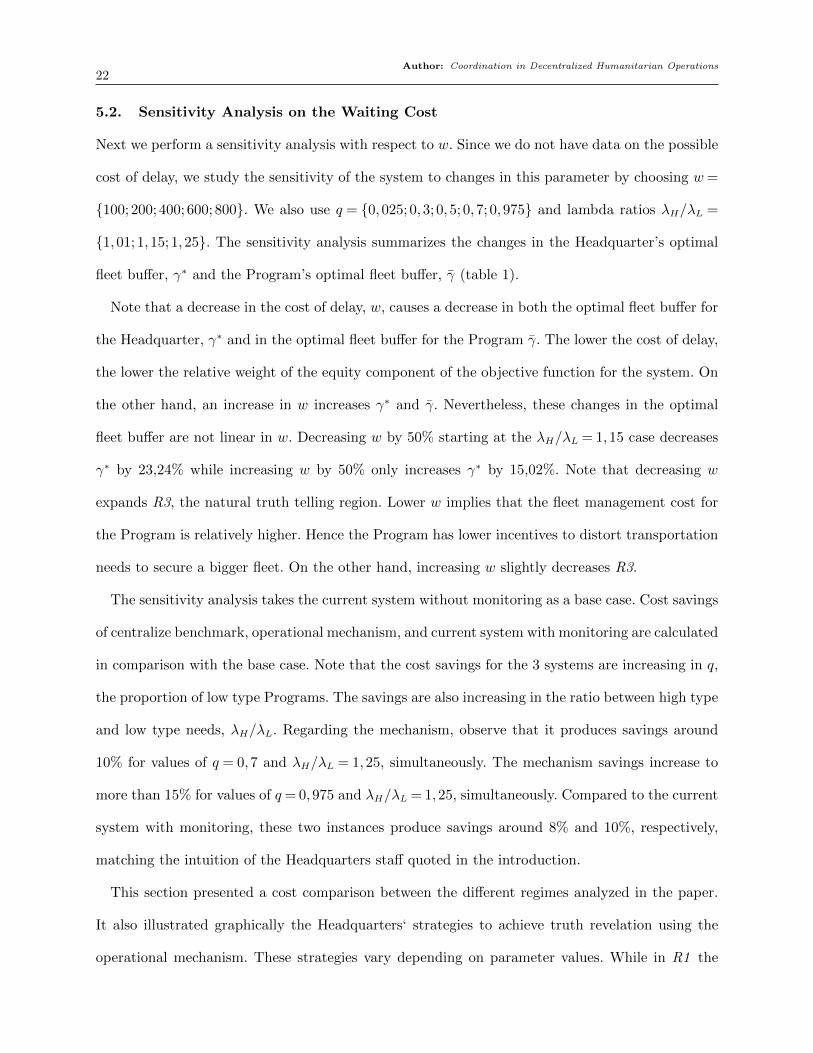
complemented with figure 4 showing the projection of γL and γH in the (λH/λL, γ) space, and

figure 5 showing the projection of γL and γH in the (q, γ) space.

First, note that the Headquarters give incentives to the low type Program in the induced truth

region R1 by choosing γ∗ <γL (figures 4a and 5a). On the other hand, to mitigate the extra-cost of

this strategy, the Headquarters simultaneously decrease the fleet buffer for the high type Program

by choosing γH < γ∗ (figure 4b and λH/λL = 1,01 in figure 5b). This way the Headquarters force

the indifference conditions γH = δH < γ∗ < γL = δL. For low values of q in R1 both γL and γH are

very close to γ∗. When q increases, the Headquarters offer a lower γH , which pushes down δL. The

Headquarters make the low type Program indifferent between revealing the truth and inflating its

needs by offering γL = δL. The extra cost of delay for the high type Program is compensated via

reduction of operating cost of the low type Programs fleet.

Second, note in figure 4a that in R2 the greater the ratio between high type and low type needs,

λH/λL, the lower the value of incentives given to the low type program. For low values of q the

Headquarter give incentives to both Program types by choosing γ∗ < γH < γL < γ̄ < δL = γ̃. To

keep the system cost balanced, the Headquarters offer the low type Program a fleet buffer greater

than γ∗, but decreasing in the proportion of low type Programs, q, (figure 5a). In fact, for large

values of q it is more efficient for the Headquarters to offer γ∗ <γL <γH < γ̄ < δL = γ̃. Nevertheless,

decreasing γL increases γ̃, such that to have the indifference condition δL = γ̃, the Headquarters

must offer the high type Program a bigger fleet buffer, up to γH = 1,7364 when q = 0,975 (figure

5b). This counterintuitive results is explained by the fact that Program cost curves are u-shaped

and do not fulfill the single crossing property. Hence, there is a region, R2, in which the difference

between types is so big that it becomes costly for the low type Program to distort its type. The

distortion would imply a marginal increase of fleet management cost relatively greater than the


(a) Low type Program (b) High type Program

Figure 3 Fleet buffers in the (λH/λL, q, γ) space

1,5

2

2,5

3

γL

0

0,5

1

1,01 1,

…1,

02 1,…

1,03 1,

…1,

04 1,…

1,05 1,

…1,

06 1,…

1,07 1,

…1,

08 1,…

1,09 1,

…1,

1 1,…

1,11

1,11

51,

12 1,…

1,13 1,

…1,

14 1,…

1,15 1,

…1,

16 1,…

1,17λH/

T1

1,151,01

R2R1

q = 0,975q = 0,7q = 0,5q = 0,3q = 0,025

1,16 1,

…1,

17 1,…

1,18 1,

…1,

19 1,…

1,2 1,…

1,21 1,

…1,

22 1,…

1,23 1,

…1,

24 1,…

1,25 1,

…1,

26 1,…

1,27 1,

…1,

28 1,…

1,29 1,

…1,

3 1,…

1,31 1,

…1,

32 1,…

/λL

1,15 1,25

T2

γ *

R3R2

(a) Low type Program

1,5

2

2,5

3

γH

0

0,5

1

1,01 1,

…1,

02 1,…

1,03 1,

…1,

04 1,…

1,05 1,

…1,

06 1,…

1,07 1,

…1,

08 1,…

1,09 1,

…1,

1 1,…

1,11 1,

…1,

12 1,…

1,13 1,

…1,

14 1,…

1,15 1,

…1,

16 1,…

1,17

λH/

T1

1,151,01

R2R1

q = 0,975q = 0,7q = 0,5q = 0,3q = 0,025

1,16 1,

…1,

17 1,…

1,18 1,

…1,

19 1,…

1,2 1,…

1,21 1,

…1,

22 1,…

1,23 1,

…1,

24 1,…

1,25 1,

…1,

26 1,…

1,27 1,

…1,

28 1,…

1,29 1,

…1,

3 1,…

1,31 1,

…1,

32 1,…

/λL

T2

1,15 1,25

γ *

R3R2

(b) High type Program

Figure 4 Fleet buffers as function of λH/λL

1

1,5

γL

λH/λL = 1,01

λH/λL = 1,15

λ /λ

0

0,5

0,02

5

0,07

5

0,12

5

0,17

5

0,22

5

0,27

5

0,32

5

0,37

5

0,42

5

0,47

5

0,30,025 0,5q

λH/λL = 1,25

0,52

5

0,57

5

0,62

5

0,67

5

0,72

5

0,77

5

0,82

5

0,87

5

0,92

5

0,97

5

0,5 0,7 0,975q

γ *

= 1,25

(a) Low Type Program

1

1,5

γH

0

0,5

0,02

5

0,07

5

0,12

5

0,17

5

0,22

5

0,27

5

0,32

5

0,37

5

0,42

5

0,47

50,30,025 0,5q

λH/λ

λH/λL = 1,15

0,52

5

0,57

5

0,62

5

0,67

5

0,72

5

0,77

5

0,82

5

0,87

5

0,92

5

0,97

50,5 0,7 0,975

λL = 1,01 λH/λL = 1,25 γ *

(b) High Type Program

Figure 5 Fleet buffers as function of q

marginal decrease in the cost of delay in relation to fleet size. The lost of information rent for the

low type Program makes the mechanism more valuable in instances where the difference between

types is big.


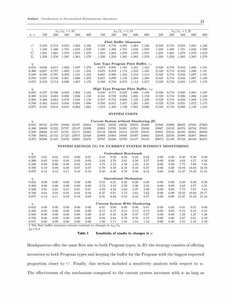
5.2. Sensitivity Analysis on the Waiting Cost

Next we perform a sensitivity analysis with respect to w. Since we do not have data on the possible

cost of delay, we study the sensitivity of the system to changes in this parameter by choosing w=

{100; 200; 400; 600; 800}. We also use q = {0,025; 0,3; 0,5; 0,7; 0,975} and lambda ratios λH/λL =

{1,01; 1,15; 1,25}. The sensitivity analysis summarizes the changes in the Headquarter’s optimal

fleet buffer, γ∗ and the Program’s optimal fleet buffer, γ̄ (table 1).

Note that a decrease in the cost of delay, w, causes a decrease in both the optimal fleet buffer for

the Headquarter, γ∗ and in the optimal fleet buffer for the Program γ̄. The lower the cost of delay,

the lower the relative weight of the equity component of the objective function for the system. On

the other hand, an increase in w increases γ∗ and γ̄. Nevertheless, these changes in the optimal

fleet buffer are not linear in w. Decreasing w by 50% starting at the λH/λL = 1,15 case decreases

γ∗ by 23,24% while increasing w by 50% only increases γ∗ by 15,02%. Note that decreasing w

expands R3, the natural truth telling region. Lower w implies that the fleet management cost for

the Program is relatively higher. Hence the Program has lower incentives to distort transportation

needs to secure a bigger fleet. On the other hand, increasing w slightly decreases R3.

The sensitivity analysis takes the current system without monitoring as a base case. Cost savings

of centralize benchmark, operational mechanism, and current system with monitoring are calculated

in comparison with the base case. Note that the cost savings for the 3 systems are increasing in q,

the proportion of low type Programs. The savings are also increasing in the ratio between high type

and low type needs, λH/λL. Regarding the mechanism, observe that it produces savings around

10% for values of q = 0,7 and λH/λL = 1,25, simultaneously. The mechanism savings increase to

more than 15% for values of q= 0,975 and λH/λL = 1,25, simultaneously. Compared to the current

system with monitoring, these two instances produce savings around 8% and 10%, respectively,

matching the intuition of the Headquarters staff quoted in the introduction.

This section presented a cost comparison between the different regimes analyzed in the paper.

It also illustrated graphically the Headquarters‘ strategies to achieve truth revelation using the

operational mechanism. These strategies vary depending on parameter values. While in R1 the


λH/λL = 1,01 λH/λL = 1,15 λH/λL = 1,25w = 100 200 400 600 800 100 200 400 600 800 100 200 400 600 800

Fleet Buffer Measures†

γ∗ 0,529 0,710 0,925 1,064 1,166 0,529 0,710 0,925 1,064 1,166 0,529 0,710 0,925 1,064 1,166γ̄ 1,246 1,468 1,701 1,840 1,939 1,246 1,468 1,701 1,840 1,939 1,246 1,468 1,701 1,840 1,939

T ‡1 1,055 1,065 1,070 1,070 1,070 1,055 1,065 1,070 1,070 1,070 1,055 1,065 1,070 1,070 1,070T2 1,220 1,250 1,265 1,265 1,270 1,220 1,250 1,265 1,265 1,270 1,220 1,250 1,265 1,265 1,270

q Low Type Program Fleet Buffer, γL0,025 0,630 0,811 1,028 1,167 1,270 0,673 0,924 1,182 1,331 1,434 0,529 0,710 0,943 1,088 1,1910,300 0,607 0,787 1,002 1,141 1,244 0,670 0,918 1,174 1,322 1,425 0,529 0,710 0,943 1,088 1,1910,500 0,588 0,767 0,982 1,121 1,223 0,665 0,909 1,162 1,310 1,413 0,529 0,710 0,943 1,087 1,1910,700 0,567 0,746 0,961 1,099 1,202 0,655 0,890 1,138 1,284 1,388 0,529 0,710 0,942 1,087 1,1900,975 0,533 0,713 0,928 1,067 1,170 0,560 0,750 0,972 1,114 1,217 0,529 0,710 0,934 1,075 1,178

q High Type Program Fleet Buffer, γH0,025 0,527 0,708 0,923 1,062 1,164 0,530 0,711 0,927 1,066 1,168 0,529 0,710 0,925 1,064 1,1670,300 0,504 0,683 0,898 1,036 1,138 0,541 0,729 0,950 1,091 1,193 0,529 0,710 0,926 1,066 1,1680,500 0,486 0,664 0,878 1,016 1,118 0,557 0,755 0,983 1,125 1,228 0,529 0,710 0,928 1,068 1,1700,700 0,465 0,643 0,856 0,994 1,096 0,594 0,815 1,057 1,201 1,304 0,529 0,710 0,931 1,072 1,1750,975 0,431 0,610 0,824 0,962 1,064 1,018 1,404 1,736 1,901 2,006 0,529 0,710 0,980 1,138 1,243

SYSTEM COSTS

q Current System without Monitoring ($)0,025 20745 21270 21846 22197 22450 23465 24022 24636 25010 25280 25308 25890 26632 27023 273030,300 20699 21222 21797 22147 22399 23263 23795 24391 24761 25028 23967 24532 26370 26756 270350,500 20666 21187 21761 22111 22363 23116 23629 24214 24579 24845 22991 23544 26180 26561 268390,700 20632 21152 21725 22075 22326 22969 23464 24036 24397 24662 22016 22556 25990 26367 266440,975 20586 21105 21676 22025 22276 22767 23236 23792 24147 24410 20674 21198 25728 26100 26375

SYSTEM SAVINGS (%) VS. CURRENT SYSTEM WITHOUT MONITORING

q Centralized Benchmark0.025 0.01 0.01 0.01 0.00 0.01 0.24 0.22 0.22 0.22 0.22 0.00 0.00 0.38 0.38 0.380.300 0.05 0.04 0.04 0.03 0.03 2.84 2.70 2.61 2.58 2.57 0.00 0.00 4.62 4.57 4.560.500 0.08 0.06 0.06 0.05 0.05 4.75 4.53 4.38 4.33 4.31 0.00 0.00 7.75 7.68 7.640.700 0.10 0.09 0.08 0.07 0.07 6.70 6.39 6.18 6.10 6.07 0.00 0.00 10.93 10.83 10.780.975 0.14 0.12 0.11 0.10 0.10 9.40 8.98 8.70 8.58 8.54 0.00 0.00 15.37 15.23 15.16

q Operational Mechanism0.025 0.00 0.00 0.00 0.00 0.00 0.23 0.21 0.20 0.20 0.20 0.00 0.00 0.38 0.38 0.380.300 0.00 0.00 0.00 0.00 0.00 2.73 2.53 2.39 2.36 2.35 0.00 0.00 4.62 4.57 4.550.500 0.01 0.01 0.01 0.01 0.01 4.58 4.24 4.03 3.97 3.96 0.00 0.00 7.75 7.67 7.640.700 0.04 0.04 0.04 0.04 0.04 6.47 6.01 5.73 5.64 5.62 0.00 0.00 10.92 10.82 10.770.975 0.13 0.11 0.10 0.10 0.09 9.31 8.84 8.53 8.42 8.37 0.00 0.00 15.37 15.23 15.16

q Current System With Monitoring0.025 0.00 0.00 0.00 0.00 0.00 0.01 0.00 0.00 0.00 0.01 0.00 0.00 0.01 0.01 0.000.300 0.00 0.00 0.00 0.00 0.00 0.17 0.15 0.14 0.13 0.13 0.00 0.00 0.44 0.44 0.440.500 0.00 0.00 0.00 0.00 0.00 0.47 0.41 0.39 0.37 0.37 0.00 0.00 1.29 1.27 1.260.700 0.00 0.00 0.00 0.00 0.00 0.94 0.84 0.78 0.76 0.75 0.00 0.00 2.67 2.61 2.590.975 0.00 0.00 0.00 0.00 0.00 1.90 1.71 1.58 1.54 1.52 0.00 0.00 5.55 5.45 5.39† The fleet buffer measures remain constant to changes in λH/λL‡q= 0,5

Table 1 Sensitivity of results to changes in w

Headquarters offer the same fleet size to both Program types, in R2 the strategy consists of offering

incentives to both Program types and keeping the buffer for the Program with the biggest expected

proportion closer to γ∗. Finally, this section included a sensitivity analysis with respect to w.

The effectiveness of the mechanism compared to the current system increases with w as long as


the parameters fall into the induced truth regions. The next section presents the conclusions and

possible avenues for future research.

6. Conclusions and Further Research

Completely informed by field research, this paper studies a decentralized two party fleet manage-

ment system in a humanitarian setting. Located in the field, Programs are service oriented and

have private information on their transportation needs. Transportation needs are fulfilled using

vehicle fleets. Located in the US or Europe, the Headquarters main objective is balancing the ser-

vice level and the operating cost of the fleet. The Headquarters can monitor the Program’s stated

transportation needs to avoid this distortion. Differences in objectives, distant geographic locations

and the private information of Programs about their transportation needs give rise to an adverse

selection problem. The Headquarters are concerned about the excess of fleet size. The Headquar-

ters are also concerned about the lack of effectiveness of monitoring tools. Finally, the Programs

are concerned about the lack of vehicles to respond to their transportation needs. We develop a

mathematically tractable model to analyze this problem while respecting exogenous constraints

that exist in the humanitarian context regarding internal budget allocation.

We find that the concerns of the two parties in the system are rational from each party’s perspec-

tive. In the current fleet management system the Headquarters monitoring effort does not dissuade

the low type Program from inflating transportation needs. This is because of the impossibility that

the Headquarters punish the distorted needs stated by the Program. We also find that the optimal

buffer factor offered by the Headquarters is lower than the optimal fleet buffer intended by the

Program. Hence, the lack of effectiveness of monitoring tools added to the incentive of the low

type Program to distort transportation needs produce a fleet excess that justifies the Headquar-

ters concerns. Finally, the Program’s concerns about not having enough vehicles to respond to its

needs are explained by the fact that its optimal fleet buffer is greater than the one offered by the

Headquarters.

Nevertheless, we find that for appropriate parameter combinations the current system has a

“natural” truth telling threshold in which the centralized benchmark solution can be achieved. In


the current fleet management system the high type Program always reveals its true transportation

needs. Otherwise, the high type Program would receive a lower fleet buffer compared to the one

offered by the Headquarters, increasing even more this Program’s costs of delay. The threshold for

natural truth telling arises when the extra fleet management cost for the fleet excess intended by the

low type Program dominates the savings from the reduction in the cost of delay. The coordination

of incentives is particularly challenging since financial transfer payments are not a viable way to

induce Program’s truth revelation in this humanitarian setting.

We propose a novel operational capacity based mechanism to coordinate incentives in this system.

In this mechanism the Headquarters offer different fleet buffer factors to the different Program

types. Additionally, the monitoring role is suppressed. We show the existence of three mutually

exclusive and collectively exhaustive regions for truth revelation under the proposed mechanism.

R1 is called the equal fleet size region. R2 is called the different fleet size region. Finally, R3 is

called the natural truth revelation region.

In the equal fleet size region the Headquarters achieve truth revelation by offering both Program

types the same fleet size. This strategy makes the low type Program indifferent between inflating

its transportation needs and revealing the truth. In the different fleet size region both Program

types are offered fleet buffers greater than optimal fleet buffer for the current system. When small

proportions of low type Programs are expected, the low type Program is offered a fleet buffer such

that this Program’s cost when inflating its needs equals the cost of revealing its true needs. When

the low type probability is high enough, it is cheaper for the Headquarters to incentivize the high

type Program. By offering the high type a bigger fleet buffer, the Headquarters increase the low

type Program’s intended fleet buffer enough to make this Program indifferent between revealing

its needs and inflating them. Finally, under some parameter combination, which is independent of

the low type probability, the system reaches a natural truth telling region. In this region, as in

the current system, the extra-cost of fleet management deters the low type Program from inflating

its transportation needs. Additionally, we show that under the mechanism the high type Program


always reveals his true transportation needs. This result is similar to the one we obtained for the

current system.

Our numerical section complements the analysis. First, it allows us to explain the lost of value

of private information for the low type program as a function of the increase in the difference with

the high type program. Second, the numerical experiments show the behavior of the system due to

changes in the cost of delay. As expected, a decrease in the cost of delay decreases the optimal fleet

buffers for the system. An increase in the cost of delay increases the fleet buffers for the system.

But the change in the optimal fleet buffers is not linear to changes in the cost of delay. Equally,

the thresholds defining the regions for truth telling are much more sensitive to decreases in the

cost of delay than they are to the increases in that cost. This is because the decrease of the cost

of delay makes the Program’s cost function flatter rapidly, increasing the size of the natural truth

revelation region.

This paper introduces a tractable mathematical model to analyze incentive alignment in decen-

tralized humanitarian settings. Some interesting extensions of this work include fleet pooling and

the joint analysis of relief and development transportation needs, which are issues faced by human-

itarian fleet managers in practice.

Appendix. ProofsProof of Lemma 1: Note that:

∂CCent(γ, )

∂γ=

[wπ′(γ)

γ−wπ(γ)

γ2+ c+ r

]√λ (16)

and:

∂CProg(γ)

∂γ=

[wπ′(γ)

γ−wπ(γ)

γ2+ c

]√λ (17)

Hence

∂CProg(γ)

∂γ=∂CCent(γ,λ)

∂γ− r√λ

∂CProg(γ)

∂γ

∣∣γ=γ∗(c,r,w)

=∂CCent(γ,λ)

∂γ

∣∣γ=γ∗(c,r,w)

− r√λ

∂CProg(γ)

∂γ

∣∣γ=γ∗(c,r,w)

= 0− r√λ< 0

Because CProg(γ) is unimodal with a finite minimum, CProg(c,w) decreases for values of γ such that γ∗(c, r,w)< γ, reachingits minimum at γ = γ̄(c,w). This implies γ∗(c, r,w)< γ̄(c,w). �

Proof of Proposition 1: Given the central benchmark solution γ∗, we have δH =λL+γ∗

√λL−λH√λH

. δH < γ∗ follows from

λL < λH . Since∂CProg(γ)

∂γ

∣∣γ=γ∗ < 0 (from lemma 1), and due to the fact that the cost function CProg(γ) is unimodal with

minimum at γ̄, and given that from lemma 1 we know that γ∗ < γ̄, it follows that CProg(γ∗)<CProg(δH). �


Proof of Proposition 2: Note that γ̄ < γ̂L. If δL < γ̂L, then CProg(δL) < CProg(γ∗). If δL = γ̂L, then CProg(δL) =CProg(γ∗). Finally, if γ̂L < δL, then CProg(γ∗)<CProg(δL). Hence, γ̂L defines the truth telling region for the low type Program.

�Proof of Proposition 3: A Program of type i would report the true transportation needs if wQ(γ) + cF (γ)≤ p(wQ(γ) +

cF (γ)) + (1− p)(wQ(δi) + cF (δi)). Since wQ(γ) + cF (γ) = p (wQ(γ) + cF (γ)) + (1− p) (wQ(γ) + cF (γ)). Using this fact we getthe truth telling condition wQ(γ)+cF (γ)≤wQ(δi)+cF (δi). The proof follows from the fact that the condition for truth tellingdoes not depend on p, the Headquarters monitoring effort. �

Proof of Proposition 4: First, we rewrite the mechanism in extended form as:

min0<γL,0<γH

E[CMec] = q

[wπ(γL)

√λL

γL+ (c+ r)(λL + γL

√λL)

](18)

+ (1− q)[wπ(γH)

√λH

γH+ (c+ r)(λH + γH

√λH)

]S.T.

(ICL) :wπ(γL)

√λL

γL+ c(λL + γL

√λL)≤

wπ(δL)√λL

δL+ c(λL + δL

√λL)

(ICH) :wπ(γH)

√λH

γH+ c(λH + γH

√λH)≤

wπ(δH)√λH

δH+ c(λH + δH

√λH)

Second, we build the mechanism’s lagrangian function L.

L(γL, γH , α1, α2) = q

[wπ(γL)

√λL

γL+ (c+ r)(λL + γL

√λL)

](19)

+ (1− q)[wπ(γH)

√λH

γH+ (c+ r)(λH + γH

√λH)

]+α1

[wπ(γL)

√λL

γL+ c(λL + γL

√λL)−

(wπ(δL)

√λL

δL+ c(λL + δL

√λL)

)]+α2

[wπ(γH)

√λH

γH+ c(λH + γH

√λH)−

(wπ(δH)

√λH

δH+ c(λH + δH

√λH)

)]

Where α1 and α2 are the lagrange multipliers for ICL and ICH , respectively. Third, we derive the first order conditions (FOC)of (19).

∂L∂γL

= (q+α1)

[wπ′(γL)

γL−wπ(γL)

γ2L

+ c

]√λL + qr

√λL−α2

[wπ′(δH)

δH−wπ(δH)

δ2H+ c

]√λL = 0

∂L∂γH

= (1− q+α2)

[wπ′(γH)

γH−wπ(γH)

γ2H

+ c

]√λH + (1− q)r

√λH −α1

[wπ′(δL)

δL−wπ(δL)

δ2L+ c

]√λH = 0

Letting f(γ) = wπ′(γ)γ− wπ(γ)

γ2+ c and dividing by

√λL in the first equation above and dividing by

√λH in the second equation

above, we can re-write the FOC as:

∂L∂γL

= (q+α1)f(γL)−α2f(δH) + qr= 0 (20)

∂L∂γH

= (1− q+α2)f(γH)−α1f(δL) + (1− q)r= 0 (21)

Note that

∂CProg(γ)

∂γ

∣∣γ=γL

= f(γL)√λL (22)

∂CCent(γ)

∂γ

∣∣γ=γL

= (f(γL) + r)√λL (23)

Replacing (22) and (23) in (20) and (21) we can re-write the FOC as:

q∂CCent(γ)

∂γ

∣∣γ=γL

+α1

∂CProg(γ)

∂γ

∣∣γ=γL

−α2

∂CProg(γ)

∂γ

∣∣γ=δH

= 0 (24)

(1− q)∂CCent(γ)

∂γ

∣∣γ=γH

+α2

∂CProg(γ)

∂γ

∣∣γ=γH

−α1

∂CProg(γ)

∂γ

∣∣γ=δL

= 0 (25)

Equations (9) and the fact that λL <λH imply that

γH < δL (26)

δH < γL (27)


Combining the definitions of δL and δH we get the useful relation:

(δL− γL)√λL = (γH − δH)

√λH (28)

Equation (28) implies the set of conditions:

γL = δL if and only if γH = δH ; γL < δL if and only if δH < γH ; δL < γL if and only if γH < δH (29)

Fourth, we characterize the induced truth telling region stated in the proposition.Characterization of R1 : Suppose 0<α1 and 0<α2. Note that 0<α1 implies CProg(γL) =CProg(δL) and 0<α2 implies

CProg(γH) =CProg(δH).There are three mutually exclusive and collectively exhaustive possibilities: either 1) δL < γ̄, or 2) δL = γ̄, or 3) γ̄ < δL.Subcase 1: δL < γ̄.Note that δL < γ̄ implies that either δL < γ̄ < γL or δL = γL. First, suppose that δL < γ̄ < γL. Then, γH < δH (due to

condition (29)). It also implies γH < δL < γ̄, and CProg(δL)<CProg(γH) follows from the fact that the Program’s cost functionis well behaved.

For CProg(γH) = CProg(λH) to be true it must be that γ̄ < δH . Also, δH < γL (from condition (26)), which implies thatCProg(δH)<CProg(γL). But CProg(γL) =CProg(δL) (because we supposed 0<α1). It follows that CProg(δH)<CProg(γL) =CProg(δL)<CProg(γH), which is a contradiction since α2 > 0 implies CProg(δH) =CProg(γH).

Second, suppose that δL = γL. This implies γH = δH (from condition (29)), and γH < γL follows (from condition (27)) andthe fact that δL = γL). This also implies δL = γL < γ̄ (from condition 0< α1). Using these facts in the first order conditions(24) and (25) and adding them we get:

q∂CCent(γ)

∂γ

∣∣γ=γL

+ (1− q)∂CCent(γ)

∂γ

∣∣γ=γH

= 0 (30)

Equation (30) only holds in three possible cases: 1) when γL = γH = γ∗, contradicting the fact γH < γL; 2) when γL < γ∗ < γH ,contradicting the fact that γH < γL, and 3) when γH < γ∗ < γL. This case is feasible and leads to the condition

δH = γH < γ∗ < γL = δL < γ̄ (31)

Subcase 2: δL = γ̄.This implies γL = δL = γ̄ (since the Program cost function is unimodal). It also implies that γH = δH < γ̄. Using these facts in

the first order conditions (24) and (25) and adding them we get again equation (30). As in the previous subcase, this equationonly holds in three possible cases: 1) when γL = γH = γ∗, contradicting the fact γH < γL; 2) when γL < γ∗ < γH , contradictingthe fact that γH < γL; and 3) when γH < γ∗ < γL. This leads to the condition:

δH = γH < γ∗ < γL = δL = γ̄ (32)

Subcase 3: γ̄ < δL. The proof for this case follows the same logic that the one for subcase 1. Note that γ̄ < δL implies eitherthat γL < γ̄ < δL or γ̄ < δL = γL. First, suppose that γL < γ̄ < δL. This implies δH < γH (from condition 29) and δH < γL < γ̄.It follows that CProg(γL)<CProg(δH) (given that the Program cost function is well behaved ). Since the cost function of theprogram is unimodal, for CProg(δH) = CProg(γH) to hold it must be that γ̄ < γH < δL. This implies CProg(γH)<CProg(δL).Hence we have CProg(γH) < CProg(δL) = CProg(γL) < CProg(δH), which contradicts the condition CProg(γH) = CProg(δH)(because we supposed 0<α2). Second, suppose that γ̄ < δL = γL. This implies δH = γH . By using those relations in first orderconditions (24) and (25) and adding them, we get equation (30). Following the same reasoning that we used in the two previoussubcases, we find the following condition:

δH = γH < γ∗ < γ̄ < γL = δL (33)

We can combine conditions (31), (32) and (33) in the following condition, which characterizes R1 in Proposition 4:

δH = γH < γ∗ < γL = δL (34)

Note that condition (34) implies that FL = FH in R1. Depending on parameter values, to make the low type Programindifferent between telling the truth and lying the Headquarters have to sacrifice some cost for the high type Program.

Characterization of R2 Suppose that 0<α1 and α2 = 0. FOC (24) and (25) become:

q∂CCent(γ)

∂γ

∣∣γ=γL

+α1

∂CProg(γ)

∂γ

∣∣γ=γL

= 0 (35)

(1− q)∂CCent(γ)

∂γ

∣∣γ=γH

−α1

∂CProg(γ)

∂γ

∣∣γ=δL

= 0 (36)

Condition (35) holds when∂CCent(γ)

∂γ

∣∣γ=γL

and∂CProg(γ)

∂γ

∣∣γ=γL

have opposite signs. This only happens when:

γ∗ < γL < γ̄ (37)

Condition (36) holds when both∂CCent(γ)

∂γ

∣∣γ=γH

and∂CProg(γ)

∂γ

∣∣γ=δL

have the same sign. This happens in two mutually

exclusive cases: 1) γH < γ∗ and δL < γ̄ simultaneously or, 2) γ∗ < γH and γ̄ < δL simultaneously.First, combining condition (37) with γH < γ∗ and δL < γ̄ simultaneously we get γ∗ < γL < γ̄, γH < γ∗ and δL < γ̄. We

supposed 0<α1. This implies CProg(γL) =CProg(δL). We also supposed α2 = 0 which implies CProg(γH)<CProg(δH). Since


γL < γ̄ and δL < γ̄, it must be that γL = δL. This implies γH = δH (from one of the conditions 29) and CProg(γH) =CProg(δH)follows, contradicting CProg(γH)<CProg(δH).

Second, combining condition (37) with γ∗ < γH and γ̄ < δL simultaneously we get γ∗ < γL < γ̄, γ∗ < γH , and γ̄ < δL.Remember the definition of γ̃L presented in (15). It must be that γ̄ < γ̃L = δL. Otherwise, the low type Program would claimhigh transportation needs violating the revelation principle. It follows that:γ∗ < γL < γ̄ < γ̃L = δL, γ∗ < γH and δH < γH . These conditions can be divided in three sub-cases. The first Sub-case is

γ∗ < γH < γL < γ̄ < γ̃L = δL, δH < γH . For low values of q, these two conditions characterize R2 in Proposition 4.The second sub-case is γ∗ < γL < γH < γ̄ < γ̃L = δL, δH < γL. The third sub-case is γ∗ < γL < γ̄ < γH < γ̃L = δL, δH < γL.

For high values of q sub-cases two and three characterize R2 in Proposition 4.

Next, we show the existence of the threshold T1 in Proposition 4. Let g(γ) = wπ′(γ)γ− wπ(γ)

γ2+ (c+ r). Note that:

qg(γL)√λL + (1− q)g(γH)

√λH

(∂γH

∂γL

)= 0 (38)

is a required condition for the FOC of the mechanism. The justification is as follows.First, for R1 we know that γL = δL and γH = δH . Replacing these values in FOC (20) and (21) we get:

(q+α1)f(γL)−α2f(γH) + qr= 0

(1− q+α2)f(γH)−α1f(γL) + (1− q)r= 0

Solving the system for α1 and α2 we get:

q(f(γL) + r) + (1− q)(f(γH) + r) = 0 (39)

The equivalence between (38) and (39) follows from the fact that in (39)∂γH∂γL

=

√λL√λH

.

Second, for R2 we know that α2 = 0. Hence, FOC (20) and (21) become:

∂L∂γL

= (q+α1)f(γL) + qr= 0

∂L∂γH

= (1− q)f(γH)−α1f(δL) + (1− q)r= 0

Then we get α1 =− q(f(γL)+r)

f(γL)such that:

(1− q)f(γH) +q(f(γL) + r)

f(γL)f(δL) + (1− q)r= 0

q(f(γL) + r) + (1− q)(f(γH) + r)f(γL)

f(δL)= 0 (40)

Remember the relation δL = γ̃L in R2. Using this we get γH =λL+γ̃L

√λL−λH√λH

. We can write∂γH∂γL

=∂γH∂γ̃L

∂γ̃L∂γL

. Note that

∂γH∂γ̃L

=

√λL√λH

and∂γ̃L∂γL

=f(γL)

f(γ̃L). The equivalence between (38) and (40) follows.

Keeping λL fixed, the next step is obtaining dC

dλH.

dC

dλH= (1− q)

[wπ(γH)

2γH√λH

+ (c+ r)

(1 +

γH

2√γH

)+ g(γH)

√λH

(∂γH

∂λH

)]

+∂γL

∂λH

[qg(γL)

√λL + (1− q)g(γH)

√λH

(∂γH

∂γL

)]Note that from condition (38) the second part of dC

dλHequals zero. Hence,

dC

dλH= (1− q)

[wπ(γH)

2γH√λH

+ (c+ r)

(1 +

γH

2√λH

)+ g(γH)

√λH

(∂γH

∂λH

)](41)

For R1 let γ1H =

λL+γ1L

√λL−λH√λH

. Then

∂γ1H

∂λH=−

λL + γL√λL

2(λH)3/2−

1

2√λH

=−λL + γ1

L

√λL +λH

2λH√λH

Such that

g(γH)√λH

(∂γH

∂λH

)=

(wπ′(γH)

γH−wπ(γH)

γ2H

+ c+ r

)(−√λH)

(λLγ1

L

√λL +λH

2λH√λH

)


=λL + γ1

L

√λL +λH

2λH

(wπ(γH)

γ2H

−wπ′(γH)

γH− (c+ r)

)Replacing for dC

dλHand simplifying we get:

dC

dλH= (1− q)

[w√λH

(π′(γ1

H)

γ1H

−π′(γ1

H)

2

)+

(wπ(γ1

H)

(γ1H)2

−wπ′(γ1

H

γ1H

)](42)

On the other hand, for R2 we have∂γ2H∂λH

=−λL+γ̃2L

√λL

2(λH )3/2− 1

2√λH

.

Following the same reasoning we used for R1 and replacing γ1H with γ2

H for R2 we get:

dC

dλH= (1− q)

[w√λH

(π′(γ2

H)

γ2H

−π′(γ2

H)

2

)+

(wπ(γ2

H)

(γ2H)2

−wπ′(γ2

H

γ2H

)](43)

Note that γ1H < γ∗ < γ2

H . If we show that dC

dλHis decreasing in γ1

H this is equivalent to show that d

dλH(C1 −C2)≥ 0. The

second part of dC

dλHin (42) is decreasing in γ1

H because it is the slope of a convex function. Next we show that π(γ)

γ− π′(γ)

2is

decreasing in γ. Note that π′(γ) = π(γ)2

γ−γπ(γ)− π(γ)

γ. Replacing we get π(γ)

γ− π′(γ)

2= 1

2

[3π(γ)

γ+ γπ(γ)− π(γ)2

γ

]. Taking the

derivative with respect to γ and simplifying we get:

−(γ2 +

6

γ2+ 3

)π(γ) +

(6

γ2+ 3

)[π(γ)]2−

2

γ2[π(γ)]3 ≤ 0

So d

dλH(C1 −C2)≥ 0 is monotonous. Now while at λH = λL we know that C1 <C2, at λH = λL + γ̄

√λL we have C1 >C2.

This implies that there exists a threshold T1 such that

C1 <C2 for λH <T1

C1 ≥C2 for λH ≥ T1 �

Proof of Corollary 1: Characterization of R3 . Suppose α1 = 0 and α2 = 0. From condition (24) we get:q∂CCent(γ)

∂γ

∣∣γ=γL

= 0. Due to the fact that CCent(γ) is unimodal we conclude that∂CCent(γ)

∂γ

∣∣γ=γL

= 0 only holds for γL = γ∗,

the centralized solution found in equation (5). A similar argument for condition (25) leads to (1− q) ∂CCent(γ)∂γ

∣∣γ=γH

= 0, which

only holds for γH = γ∗. Then the solution is γL = γH = γ∗. The Headquarters propose γL = γH = γ∗ when γ̃L < δL. The explana-

tion is as follows. Since CProg(γ) is unimodal with minimum in γ̄, and γ∗ < γ̄ it must be that γ̄ < γ̃L. Hence 0<∂CProg(γ)

∂γ

∣∣γ=γ̃

.

Therefore, γ̃ < δL implies that CProg(γ∗) =CProg(γ̃)<CProg(δL). On the other hand, the high type Program would report its

true needs since δH < γL = γ∗ and∂CProg(γ)

∂γ

∣∣γ=γ∗ < 0 implying CProg(γ∗)<CProg(δH). �

References

Altay, N., Green III, W.G. 2006. OR/MS research in disaster operations management European Journal of

Operational Research 175, 475–493.

Barbarosoglu, G., L. Ozdamar, A. Cevik. 2002. An interactive approach for hierarchical analysis of helicpter

logistics in disaster relief operations. European Journal of Operational Research, 140 (1), 118–133.

Barbarosoglu, G., Y. Arda. 2004. A two-stage stochastic Programming framework for transportation planning

in disaster response. Journal of the Operational Research Society. 55 (1), 43–53.

Batta, R., N.R. Mannur. 1990. Covering-location models for emergency situations that require multiple

response units. Management Sci. 36 (1), 16–23.

Beamon, B.M., S.A. Kotleba. 2006. Inventory modelling for complex emergencies in humanitarian relief

operations. International Journal of Logistics: Research and Applications. 9 (1), 1–18.

Bernstein, F., A. Federgruen. 2003. Pricing and replenishement strategies in a distribution system with

competitive retailers. Operations Research. 51(3) 409–426.


Bookbinder, J.H., D.L. Martell. 1979. Time-dependent queueing approach to helicopter allocation for forest

fire initial-attack INFOR 17(1) 58–70.

Borst, S. Mandelbaum, A. Reiman. 2004. Dimensioning large call centers. Operations Research. 52(1) 17–34.

Campbell A.M., D. Vanderbussche, W. Hermann. 2008. Routing for relief efforts. Transportation Sci. 42(2)

127–145.

Cachon, G.P., M.A. Lariviere. 2005. Supply chain coordination with revenue-sharing contracts: strengths

and limitations. Management Sci. 51(1) 30–44.

Cachon, G.P., Tearwiesch, C. 2009. Matching supply with demand. An introduction to operations manage-

ment. McGraw-Hill. Second Edition - International Edition.

Chang, M-S, Y-L. Tseng, J-W Cheng. 2007. A scenario planning approach for the flood emergency logistics

preparation problem under uncertainty. Transportation Research Part E. 43 737-754

Chiu, Y.C., H. Zheng. 2007. Real-time mobilization decisions for multi-priority emergency response resources

and evacuation groups: Model formulation and solution Transportation Research Part E. 43 710-736

Corbett, C.J., X. de Groote. 2000. A supplier’s optimal quantity discount policy under asymmetric informa-

tion. Management Sci. 46(3) 444–450.

Cova, T.J., J.P. Johnson. 2003. A network flow model for lane-based evacuation routing Transportation

Research Part A. 37 579–604

Dasgupta, P., P. Hammon, E. Maskin. 1979. The Implementation of social choice rules: some general results

on incentive compatibility The Review of Economic Studies, 46(2) 185–216

De Angelis, V. M. Mecoli, C. Nikoi, G. Storchi. 2007. Multiperiod integrated routing and scheduling of World

Food Programme cargo planes in Angola. Computers & Operations Research. 34 1601–1615

Grassmann, W.K. 1988. Finding the right number of servers in real-world queuing systems. Interfaces. 18(2)

94–104.

Green, L.V.. 1984. A multiple dispatch queueing model of police patrol operations. Management Sci. 30(6)

653–664.

Green, L.V., P. Kolesar. 1984a. The feasibility of one-officer patrol in New York City. Management Sci. 30(8)

964–981.


Green, L.V., P. Kolesar. 1984b. A comparison of the multiple dispatch and M/M/c priority queueing models

of police patrol. Management Sci. 30(6) 665–670.

Green, L.V., P. Kolesar. 1989. Testing the validity of a queueing model of a police patrol. Management Sci.

35(2) 127–148.

Green, L.V., P. Kolesar. 2004. Improving emergency responsiveness with management science. Management

Sci. 50(8) 1001–1014.

Green, J., J.J. Laffont. 1977. Characterization of satisfactory mechanisms for the revelation of preferences

for public goods. Econometrica. 45(2) 427–438.

Halfin, S. W. Whitt. 1981. Heavy-traffic limits of queues with many exponential servers. Operations Research.

29(3) 567–588

Harris, M., R.M. Townsend. 1981. Resource Allocation Under Asymmetric Information Econometrica. 49(1)

33–64

Hasija, S., E.J. Pinker, R.A. Shumsky. 2005. Staffing and routing in a two-tier call centre. Int. J. Operational

Research. 1(1) 8–29 .

Hasija, S., E.J. Pinker, R.A. Shumsky. 2008. Call center outsourcing contracts under information asymmetry.

Management Sci. 54(4) 793–807.

Ignall, E., Carter, G., Rider, K. 1982. An algorithm for the unitial dispatch of fire companies. Management

Sci. 28(4) 366-378

Jia, H., F. Ordonez, M. Dessouky. 2007. A modeling framework for facility location of medical services for

large-scale emergencies IIE Transactions. 39 41-55

Kolesar, P., E. W. Blum. 1973. Square root laws for fire engine response distances. Management Sci. 19(2)

1368–1378.

Krishnan, H., R. Kapuscinski, D.A. Butz. 2007. Coordinating contracts for decentralized supply chains with

retailer promotional effort. Management Sci. 50(1) 48–63.

Lindenberg, M. 2001. Are we at the cutting edge of the blunt blunt edge? Improving NGO organizatinal

performance with private and public sector strategic management frameworks. Nonprofit Management

& Leadership. 11(3) 247–270.


Mannell, J. 2010. Are the sectors compatible? International development work and lessons for a business–

profit partnership framework. Journal of Applied Social Psychology. 40(5) 1106–1122.

Maskin, E., Riley, J. 1984. Monopoly with Incomplete Information. The RAND Journal of Economics. 15(2)

171–19

Myerson, R. B. 1979. Incentive Compatibility and the Bargaining Problem. Econometrica. 47(1) 61–73

Ozdamar, L., E. Ekinci, B. Kucukyazici. 2004. Emergency logistics planning in natural disasters Annals of

Operations Research. 129 217–245

Pedraza Martinez, A.J., O. Stapleton, L.N. Van Wassenhove. 2010. Field vehicle fleet management in human-

itarian operations: a case-based approach. Journal of Operations Management Jul 2011, 29 (5) 404–421

Pedraza Martinez, A.J., L.N. Van Wassenhove. 2010. Vehicle replacement in the International Committee of

the Red Cross. Production and Operations Management (Forthcoming).

Pasternack, B.A. 1985. Optimal pricing and return policies for perishable commodities. Marketing Sci. 4(2)

166–176.

Regnier, E. 2008. Public evacuation decisions and hurricane track uncertainty. Management Sci. 54 (1) 16–28

Saadatseresht, M., A. Mansourian, M. Taleai. 2009. Evacuation planning using multiobjective evolutionary

optimization approach. European Journal of Operational Research. 198 305–314

Salmeron, J., A. Apte. 2009. Stochastic optimization for natural disaster asset prepositioning. Production

and Operations Management. 19(5) 561–574

Sheu, J.B. 2007. An emergency logistics distribution approach for quick response to urgent relief demand in

disasters. Transportation Research E. 43 687 – 709

Singer, M., P. Donoso. 2008. Assessing an ambulance service with queuing theory. Computers & Operations

Research. 35 2549–2560

Stepanov. A., J.M. Smith. 2009. Multi-objective evacuation routing in transportation networks. European

Journal of Operational Research. 198 435–446

Su, X., S.A. Zenios. 2006. Recipient choice can address the efficiency-equity trade-off in kidney transplanta-

tion: a mechanism design model. Management Sci. 52(11) 1647–1660.

Taylor, T. 2002. Supply chain coordination under channel rebates with sales effort effects. Management Sci.

48(8) 992–1007.


Thomas, A., L. Kopczak. 2005. From logistics to supply chain management: the path forward in the human-

itarian sector. Fritz Institute White Paper

Van Wassenhove, L. N. 2006. Humanitarian aid logistics: supply chain management in high gear. Journal of

the Operational Research Society 57 475–489.

Whitt, W. 1992. Understanding the efficiency of multi-server service systems. Management Sci. 38(5) 708–

723.

Yi, W., L. Ozdamar. 2007. A dynamic logistics coordination model for evacuation and support in disaster

response activities. European Journal of Operational Research. 179(3) 1177–1193.

Documents

Fleet Management Coordination in Decentralized ...Author: Coordination in Decentralized Humanitarian Operations 3 to the cost of delay than to the eet management cost. The bigger the