IEEE TRANSACTIONS ON 1 3D Decentralized Prioritized Motion ...dpanagou/assets/documents/XMa_TCST… · 3D Decentralized Prioritized Motion Planning and Coordination for High-Density

IEEE TRANSACTIONS ON 1

3D Decentralized Prioritized Motion Planning andCoordination for High-Density Operations of Micro

Aerial VehiclesXiaobai Ma, Ziyuan Jiao, Zhenkai Wang and Dimitra Panagou∗

Abstract—This paper presents a decentralized motion planningmethod for multiple aerial vehicles moving among 3D polygonalobstacles resembling an urban-like environment. The algorithmcombines a prioritized A? algorithm for high-level planning,along with a coordination method based on barrier functionsfor low-level trajectory generation and vehicle control. To thisend we extend the barrier functions method developed in ourearlier work so that it treats 2D and 3D polygonal obstacles, andgenerates collision-free trajectories for the multi-agent system.We furthermore augment the low-level trajectory generationand control with a prioritized A? path planning algorithm, inorder to compute waypoints and paths that force agents oflower priority to avoid the paths of agents of higher priority,reducing thus congestion. This feature enhances further theperformance of the barrier-based coordination, and results inshorter paths and time to the goal destinations. We finally extendthe proposed control design to agents of constrained double-integrator dynamics, compared to the single-integrator case inour earlier work. We assume that the obstacles are known to theagents, and that each agent knows the state of other agents lyingin its sensing area. Simulation results in 2D and 3D polygonalenvironments, as well as experimental results with micro aerialvehicles (quadrotors) in an indoor lab environment demonstratethe efficacy of the proposed approach.

I. INTRODUCTION

Motion planning is a core, active research topic in therobotics and control systems communities, that becomes par-ticularly challenging for multi-robot systems [1], [2]. Mo-tion planning for a single robot is typically treated with (i)sampling-based methods, including probabilistic roadmaps [3],and rapidly-exploring random trees [4], [5], (ii) Lyapunov-based methods, including either the definition of closed-formfeedback motion plans via potential functions or vector fields,or computation of Lyapunov-based feedback motion plans viasum-of-squares programming [6], [7], (iii) graph search anddecision theory, see also [8], [9] for an extensive presentationon motion planning methods.

*Corresponding authorXiaobai Ma is a Graduate Student with the Department of Aeronautics and

Astronautics, Stanford University, USA; [email protected] Jiao is a Graduate Student with the Department of Mechanical En-

gineering, University of Michigan, Ann Arbor, USA; [email protected] Wang is a Graduate Student with the Department of Aeronautics

and Astronautics, Stanford University, USA; [email protected] Panagou is an Assistant Professor with the Department of

Aerospace Engineering, University of Michigan, Ann Arbor, MI, USA;[email protected].

Dimitra Panagou would like to gratefully acknowledge the support ofthe NASA Grant NNX16AH81A. This work was in part done during theUniversity of Michigan SURE (Summer Undergraduate REsearch) Project ofthe first and second author.

Each method has its own merits and disadvantages.Sampling-based methods typically produce paths that needto be smoothened prior to execution, while the trajectorygeneration for agents with complex dynamics is not straight-forward; furthermore, the convergence to the desired goal isprobabilistic. Potential functions [10] unify path planning andtrajectory generation, but they typically exhibit local minimawhich result in trajectories getting stuck away from the desiredgoal, while special forms of local-minima free functionstypically require tweaking of certain parameters to producecollision-free and convergent trajectories [11], [12]. Reactivemethods have been refined over the years to overcome thedeficiencies of gradient-based solutions [13]. In [14], theauthors introduce the notion of a “reciprocal velocity obstacle”which guarantees oscillation-free motion; however, typicallysuch methods do not consider global path optimization. Inaddition, the traditional discrete planning methods such asrapidly-exploring random trees and probabilistic roadmapsdo not scale well for multi-agent problems as they requireextensive computation when directly used in high-dimensionalspaces. The Lazy Probabilistic Roadmap Method [15], andMAPP [16] aim to reduce the computational demand of suchmethods; however, collision avoidance in these approaches isinherently treated in a discrete manner, i.e., agents can onlyswitch between nodes, but do not fully use the space betweennodes. In contrast to those solutions, potential function andvector field based methods can provide a continuous avoidingbehavior. More recently, safety verification of hybrid systemsby means of barrier certificates [17], [18] has motivated andbeen used in the computation of Lyapunov-based feedbackcontrollers for classes of nonlinear systems by sum-of-squaresprogramming [19], [20]. Here we adopt an approach thatutilizes barrier functions and seeks to render certain levelsets as positively invariant sets, but instead of computing theLyapunov barrier (or barrier certificate), we utilize a specificgiven form for the candidate Lyapunov barrier function.

In addition to the previous methods that have been mostlyused in single-agent settings, prioritized planning has been apopular method in the multi-robot motion planning literature,and various approaches on assigning priorities are described,for instance, in [21]–[28]. In a prioritized approach, each robothas its own priority, and computes its path based on the relativeorder imposed by their priorities. Hence the resulting path foreach robot avoids static obstacles on the map as well as therobots with higher priority in its communication region, whichare considered as dynamic obstacles.


A. Motivation and Problem Challenges

This work presents a decentralized prioritized algorithm forthe motion planning and coordination of multiple agents in3D obstacle environments, which combines a prioritized A?

algorithm for the high-level path planning, and a low-levelbarrier-based control method for multi-agent coordination andcollision avoidance.

We are primarily motivated by applications relevant tothe future Unmanned Aircraft Systems Traffic Managementin low-altitude airspace. Arguably, the problems of sense-and-avoid, separation assurance, and trajectory prediction andgeneration have been well-studied research topics both inthe robotics field, as well as in the aerospace field, see forinstance [29]–[41]. Nevertheless, the envisioned autonomouslow-altitude flight of small Unmanned Aerial Systems (UAS)in urban environments poses both technological and funda-mental challenges, that make the problem different comparedto manned flight in the current airspace structure, or comparedto 2D robot deployments.

Towards this end, in this paper we build protocols andalgorithms for the automated 3D trajectory generation andconflict resolution for small UAS (i) in cluttered polygonalenvironments that resemble an urban environment under givenconstraints on the sensing, communication and mobility ofthe agents, (ii) in making the trajectory generation for eachagent anticipatory of the others’ actions, so that areas of highcongestion are avoided.

The proposed approach combines a priority-based high-level path planning and a barrier-based low-level coordina-tion and control scheme. The low-level reactive coordinationscheme offers a computationally inexpensive way to resolveconflicts, however with the caveat that it typically results inunnecessarily longer (i.e., suboptimal) paths, that often sufferfrom chattering. Thus a prediction or look-ahead capabilityin the decision-making processes of the agents is beneficialfor efficient mission accomplishment. For this reason weaugment the low-level coordination with the proposed priority-based high-level planning in order to improve the performanceof the system when it comes to high-density operations ofautonomous agents, such as small micro aerial robots incluttered and congested 2D and 3D environments.

B. Contributions

More specifically, we propose a two-level strategy forthe decentralized motion planning, trajectory generation andcontrol of micro aerial vehicles in 3D polygonal obstacleenvironments (Fig. 1), which combines a prioritized A? high-level path planner along with a low-level controller that isbased on barrier functions for multi-agent coordination. Wefirst build upon the method in [42] and modify it to accountfor known polygonal obstacles in 2D and 3D environments,as well as for agents of double integrator dynamics. Wealso define a prioritized A? algorithm to plan paths for theagents that result in reduced traffic congestion in confinedenvironments. The prioritized A? is triggered whenever agentsbecome connected, and results in paths for the lower priorityagents that are anticipatory of the paths of the agents of

Fig. 1. The considered scenario: micro aerial vehicles flying in an urbanarea towards goal destinations while avoiding obstacles (other quadrotors,buildings).

higher priority. This way the agents of lower priority avoidthe areas-to-be-occupied in a short time horizon ahead by theagents of higher priority, with the effect of reducing trafficcongestion. System safety is taken care of by the low-levelcontrol using a semi-cooperative coordination protocol builtupon our work in [43]. In effect, the proposed two-levelstrategy combines the advantages of the utilized methods whileovercoming their disadvantages. Namely, the decentralizedbarrier functions provide safe directions of motion for theagents, and furthermore guide the design of their velocityadjustment algorithms for conflict resolution and collisionavoidance. The derived semi-cooperative protocol guaranteesthe generation of collision-free trajectories without necessarilyforcing all agents to participate in conflict resolution (hencethe term semi-cooperative). This way, the trajectory gener-ation does not suffer from the computational load of purediscrete path-planning methods in high-dimensional spaces. Inaddition, the prioritized A? algorithm provides waypoints thateliminate the “getting stuck” situation often encountered inpure potential function-based methods, and forces agents oflower priority to avoid the paths of agents of higher priority,resulting thus in shorter paths that favor the reduction of trafficjam. Finally, the low-level control design in this paper isbased on double-integrator dynamics with acceleration bounds,a consideration which is different compared to our earlierrelevant work [42], [43] that addresses kinematic agent modelsonly. Experimental results with three quadrotors accompanythe computer simulations and demonstrate the efficiency ofthe proposed approach in realistic settings.

Part of this work has been presented in [44]. Compared tothe conference version, here we consider agents of constraineddouble-integrator dynamics, instead of agents governed bysingle-integrator dynamics, and provide all the theoreticalproofs that were omitted in the conference version in theinterest of space.

The paper is organized as follows: Section II gives themathematical modeling and an overview of the proposedapproach. The high-level prioritized planning and the low-levelcoordination are given in Sections III and IV, respectively,while Section V presents their extension to 3D environments.


Simulation results in 2D and 3D environments, including acomparison of the prioritized A? algorithm with the standardA? algorithm, are given in Section VI, whereas experimentalresults using quadrotors are presented in Section VII. SectionVIII summarizes our findings and thoughts on future research.Finally, the Appendix reviews the standard A? planning algo-rithm.

II. MODELING AND PROBLEM STATEMENT

The equations describing the motion of a quadrotor withmass m and inertia matrix J expressed in the body-fixed frameare given as:

rn = C(η)nb vb, (1a)

vb = ωb × vb +m−1F b, (1b)

η = R ωb, (1c)

ωb = J−1(−ωb × Jωb +M b), (1d)

where rn is the position vector of the center of gravity ofthe quadrotor with respect to (w.r.t.) the navigational (i.e.,an inertial) frame of reference, vb is vector of translational(linear) velocity of the quadrotor expressed in the body frameof reference, η =

[φ θ ψ

]Tis the attitude representation

of the body frame relative to the navigational frame in 3-2-1 Euler angles (yaw (ψ), pitch (θ), roll (φ)), C(η)nb isthe rotation matrix in 3-2-1 Euler angle representation fromthe body frame to the navigational frame, ωb is the angularvelocity of the vehicle expressed in the body frame, F b is thetotal force including the motor trust, gravity and aerodynamicforces expressed in the body frame, and M b is the totaltorque expressed in the body frame, containing the momentsgenerated by thrust, gravity and aerodynamic forces, and

R =

[1 sinφ tan θ cosφ tan θ0 cosφ − sinφ0 sinφ sec θ cosφ sec θ

].

In the subsequent simulation and experimental trials, themotor regulation as well as the attitude control of the quadrotorare implemented by the simulator and the vehicle’s on-boardcontroller, respectively. Hence our planning, coordination andcontrol design focuses on computing and implementing trans-lational (linear) velocity and acceleration commands to thequadrotor.

We furthermore assume that the roll, pitch, and yaw anglesremain close to zero during flight, so that the equations ofmotion can be approximated via double integrator dynamics:

r = v, (2a)v = a, (2b)

where r is the position vector, v is the linear velocity vector,and a is the linear acceleration vector, all expressed w.r.t. thenavigational frame.

We consider N quadrotors, called thereafter agents, underdouble-integrator dynamics (2), that are deployed in a known2D workspace W with M static polygonal obstacles. Eachagent i ∈ {1, . . . , N} is modeled as a circular disk of radiusra and is assigned a unique, static priority, that is used in thehigh-level planning mode, as will be explained in the sequel.

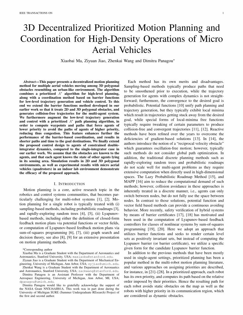
Fig. 2. Each agent i can measure the position rj of any agent j lying withindistance dij ≤ Rs, i.e., within its sensing region. Furthermore, each followeragent i receives the linear velocity uj of any agent j lying within distancedij ≤ Rc, i.e., within its communication region. The radius Rz is used inthe definition of the blending function σij(·) in (9).

We assume that each agent: (i) knows its own position ri w.r.t.the inertial frame, (ii) knows its velocity vector vi w.r.t. theinertial frame, (iii) measures the position rj of agents j 6= ilying in its sensing region, realized as a circular disk of radiusRs, and (iv) exchanges information on linear velocities withagents k 6= i lying in its communication region, realized asa circular disk of radius Rc < Rs, see also Figure 2. A pairof agents i and j is said to be connected if the inter-agentdistance dij = ‖ri − rj‖ is less or equal than the sensingradius Rs, i.e., dij ≤ Rs.

Each agent is assigned a goal location rgi =[xgi ygi

]Tin the free space and needs to move there while avoiding staticobstacles and other agents.

A. Overview of the Two-Level Approach

The proposed approach comprises a low-level coordinationand control method, as well as a high-level prioritized pathplanning method.

The purpose of the prioritized high-level planning is to makeagents of lower static priority avoid the nodes to be occupiedby the nearby agents of higher static priority, providing thus away of anticipating and avoiding traffic congestion. Towardsthis end, each agent in a connected group computes a path toits goal by executing an A? planning algorithm in a sequentialspirit: starting from the agent of highest priority in the group,each agent i re-plans a path to its goal location while takinginto account the location of the static obstacles and the first nnodes in the waypoint lists of the agents of higher priority, andcommunicates the first n nodes of its new path to the agentslower priority. Hence, by avoiding the future nodes of nearbyagents with higher priorities, traffic congestion is anticipatedand avoided by the agents of lower priority. The high-levelplanning for each agent is triggered at the time instances when


a new agent of higher priority is added to its set of neighboringagents.

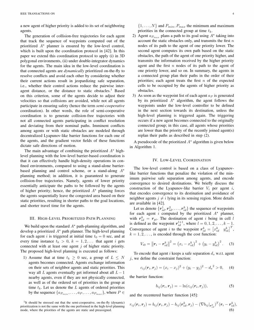
The generation of collision-free trajectories for each agentthat track the sequence of waypoints computed out of theprioritized A? planner is ensured by the low-level control,which is built upon the coordination protocol in [42]. In thispaper we extend this coordination protocol to apply (i) in 3Dpolygonal environments, (ii) under double-integrator dynamicsfor the agents. The main idea in the low-level coordination isthat connected agents are dynamically prioritized on-the-fly toresolve conflicts and avoid each other by considering whethertheir current actions result in jeopardizing safe separation,i.e., whether their control actions reduce the pairwise inter-agent distance, or the distance to static obstacles.1 Basedon this criterion, some of the agents decide to adjust theirvelocities so that collisions are avoided, while not all agentsparticipate in ensuring safety (hence the term semi-cooperativecoordination). In other words, the role of semi-cooperativecoordination is to generate collision-free trajectories withnot all connected agents participating in conflict resolutionand deviating from their nominal paths. Imminent conflictsamong agents or with static obstacles are modeled throughdecentralized Lyapunov-like barrier functions for each one ofthe agents, and the gradient vector fields of these functionsdictate safe directions of motion.

The main advantage of combining the prioritized A? high-level planning with the low-level barrier-based coordination isthat it can effectively handle high-density operations in con-fined environments, compared to using a stand-alone barrier-based planning and control scheme, or a stand-along A?

planning method; in addition, it is guaranteed to generatecollision-free trajectories. Namely, agents of lower priorityessentially anticipate the paths to be followed by the agentsof higher priority; hence, the prioritized A? planning forcesthe agents sequentially leave the congested area based on theirstatic priorities, resulting in shorter paths to the goal locations,and shorter travel time for the agents.

III. HIGH-LEVEL PRIORITIZED PATH PLANNING

We build upon the standard A? path-planning algorithm, anddevelop a prioritized A? path planner. The high-level planningfor each agent i is triggered at initial time t0 = 0 sec, and atevery time instance tk > 0, k = 1, 2, . . . that agent i getsconnected with at least one agent j of higher static priority.The proposed high-level planning is executed as follows:

1) Assume that at time tk ≥ 0 sec, a group of L ≤ Nagents becomes connected. Agents exchange informationon their sets of neighbor agents and static priorities. Thisway all L agents eventually get informed about all L− 1nearby agents, even if they are not physically connected,as well as of the ordered set of priorities in the group attime tk. Let us denote the L agents of ordered prioritiesby the sequence {aPmin , . . . , aP , . . . , aPmax}, where P ∈

1It should be stressed out that the semi-cooperative, on-the-fly (dynamic)prioritization is not the same with the one performed in the high-level planningmode, where the priorities of the agents are static and preassigned.

{1, . . . , N} and Pmin, Pmax the minimum and maximumpriorities in the connected group at time tk.

2) Agent aPmaxplans a path to its goal using A? taking into

account the static obstacles only, and transmits the first nnodes of its path to the agent of one priority lower. Thesecond agent computes its own path based on the staticobstacles, the path of the agent of one priority higher, andtransmits the information received by the higher priorityagent and the first n nodes of its path to the agent ofone priority lower, and so on. In summary, the agents ina connected group plan their paths in the order of theirpriorities; each agent treats the first n of the expectedcells to be occupied by the agents of higher priority asobstacles.

3) As soon as the waypoint list of each agent aP is generatedby its prioritized A? algorithm, the agent follows thewaypoints under the low-level controller to be definedin the next section towards its destination, unless thehigh-level planning is triggered again. The triggeringoccurs if a new agent becomes connected to the originallyconnected group; in this case, all agents whose prioritiesare lower than the priority of the recently joined agent(s)replan their paths as described in step (2).

A pseudocode of the prioritized A? algorithm is given belowin Algorithm 1.

IV. LOW-LEVEL COORDINATION

The low-level control is based on a class of Lyapunov-like barrier functions that penalize the violation of the min-imum pairwise safe separation among agents, and encodeconvergence to desired destinations. We briefly discuss theconstruction of the Lyapunov-like barrier Vi per agent i,that encodes convergence to its destination and avoidance ofneighbor agents j 6= i lying in its sensing region. More detailsare available in [42].

Let us denote {r1id, r

2id, . . . , r

kid} the sequence of waypoints

for each agent i computed by the prioritized A? planner,with rkid = rgi. The destination of agent i being in cell lis defined as the waypoint rl+1

id , where l = 0, 1, 2, . . . , k − 1.Convergence of agent i to the waypoint rkid =

[xkid ykid

]T,

k = 1, 2, . . . , is encoded through the cost function:

Vi0 =∥∥ri − rkid∥∥2

=(xi − xkid

)2+(yi − ykid

)2. (3)

To encode that agent i keeps a safe separation ds w.r.t. agentj, we define the constraint function:

cij(ri, rj) = (xi − xj)2 + (yi − yj)2 − ds2 > 0, (4)

the barrier function:

bij(ri, rj) = − ln(cij(ri, rj)), (5)

and the recentered barrier function [45]:

rij(ri, rj) = bij(ri, rj)− bij(rkid, rj)− (∇bij |rkid

)T (ri − rkid),(6)


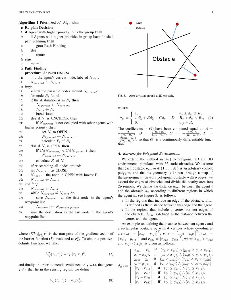
Algorithm 1 Prioritized A? Algorithm1: Re-plan Decision2: if Agent with higher priority joins the group then3: if Agents with higher priorities in group have finished

path planning then4: goto Path Finding5: else6: return7: else8: return9: Path Finding

10: procedure A? PATH FINDING11: find the agent’s current node, labeled Nstart12: Ncurrent ← Nstart13: loop:14: search the passable nodes around Ncurrent:15: for node Ni found:16: if the destination is in Ni then17: Ni,parent ← Ncurrent18: Nend ← Ni19: break loop20: else if Ni is UNCHECK then21: if Ncurrent is not occupied with other agents with

higher priority then22: set Ni to OPEN23: Ni,parent ← Ncurrent24: calculate Fi of Ni25: else if Ni is OPEN then26: if Gi(Ncurrent) < Gi(Ni,parent) then27: Ni,parent ← Ncurrent

28: calculate Fi of Ni29: after searching all nodes around:30: set Ncurrent as CLOSE31: Nnext ← the node in OPEN with lowest F.32: Ncurrent ← Nnext33: end loop34: Ncurrent ← Nend35: while Ncurrent 6= Nstart do36: save Ncurrent as the first node in the agent’s

waypoint list37: Ncurrent ← Ncurrent,parent

38: save the destination as the last node in the agent’swaypoint list

where (∇bij |rkid

)T is the transpose of the gradient vector ofthe barrier function (5), evaluated at rkid. To obtain a positive-definite function, we take:

V ′ij(ri, rj) = rij(ri, rj)2, (7)

and finally, in order to encode avoidance only w.r.t. the agentsj 6= i that lie in the sensing region, we define:

Vij(ri, rj) = σijV′ij , (8)

Fig. 3. Area division around a 2D obstacle.

where:

σij =

1, ds ≤ dij ≤ Rz,Ad3

ij +Bd2ij + Cdij +D, Rz < dij < Rs,

0, dij ≥ Rs.(9)

The coefficients in (9) have been computed equal to: A =− 2

(Rz−Rs)3 , B = 3(Rz+Rs)(Rz−Rs)3 , C = − 6RzRs

(Rz−Rs)3 , D =R2

s(3Rz−Rs)(Rz−Rs)3 , so that (9) is a continuously differentiable func-

tion.

A. Barriers for Polygonal Environments

We extend the method in [42] to polygonal 2D and 3Denvironments populated with M static obstacles. We assumethat each obstacle om, m ∈ {1, . . . ,M} is an arbitrary convexpolygon, and that its geometry is known through a map ofthe environment. Given a polygonal obstacle with p edges, weextend the edges of obstacles and divide the nearby area into2p regions. We define the distance diom between the agent iand the obstacle om according to different regions in whichthe agent is, see Figure 3, as follows:• In the regions that include an edge of the obstacle, diom

is defined as the distance between this edge and the agent.• In the regions that include a vertex but not edges of

the obstacle, diom is defined as the distance between thevertex and the agent.

An example on defining the distance between an agent i anda rectangular obstacle oj with 4 vertices whose coordinatesare ro11 =

[xoj1 yoj1

]T, ro12 =

[xoj1 yoj2

]T, ro21 =[

xoj2 yoj1]T

and ro22 =[xoj2 yoj2

]T, where xoj1 < xoj2

and yoj1 < yoj2, is given as follows:

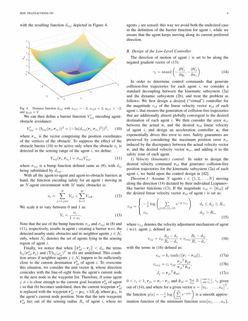
dioj =

xoj1 − xi, if (xi < xoj1) ∧ (yoj1 < yi < yoj2),xi − xoj2, if (xi > xoj2) ∧ (yoj1 < yi < yoj2),yoj1 − yi, if (yi < yoj1) ∧ (xoj1 < xi < xoj2),yi − yoj2, if (yi > yoj2) ∧ (xoj1 < xi < xoj2),‖ri − ro11‖, if (yi ≤ yoj1) ∧ (xi ≤ xoj1),‖ri − ro12‖, if (yi ≥ yoj2) ∧ (xi ≤ xoj1),‖ri − ro21‖, if (yi ≤ yoj1) ∧ (xi ≥ xoj2),‖ri − ro22‖, if (yi ≥ yoj2) ∧ (xi ≥ xoj2),


with the resulting function dioj depicted in Figure 4.

Fig. 4. Distance function dioj with xoj1 = −2, xoj2 = 2, yoj1 = −2,and yoj2 = 2

We can then define a barrier function V ′ioj encoding agent-obstacle avoidance:

V ′ioj = (bioj(ri, roj ))2 = (− ln(dioj(ri, roj )2))2, (10)

where roj is the vector comprising the position coordinatesof the vertices of the obstacle. To suppress the effect of theobstacle barrier (10) to be active only when the obstacle oj isdetected in the sensing range of the agent i, we define:

Vioj(ri, roj ) = σiojV′ioj , (11)

where σioj is a bump function defined same as (9), with dijbeing substituted by dioj .

With all the agent-to-agent and agent-to-obstacle barriers athand, the function encoding safety for an agent i moving inan N -agent environment with M static obstacles is:

νi =

N∑j=1,j 6=i

Vij +

M∑k=1

Viok. (12)

We scale it to vary between 0 and 1 as:

Vi =νi

1 + νi. (13)

Note that the use of the bump functions σij and σioj in (8) and(11), respectively, results in agent i creating a barrier w.r.t. thedetected nearby static obstacles and its neighbor agents j ∈ Nionly, where Ni denotes the set of agents lying in the sensingregion of agent i.

Finally, we notice that when∥∥rkid − rj∥∥ < ds, the terms

bij(rkid, rj) and (∇bij |rk

id)T in (6) are undefined. This condi-

tion arises if neighbor agents j ∈ Ni happen to lie sufficientlyclose to the current destination rkid of agent i. To overcomethis situation, we consider the unit vector η, whose directioncoincides with the line-of-sight from the agent’s current nodeto the next node in the waypoint list. Therefore, if some agentj 6= i is close enough to the current goal location rkid of agenti so that (6) becomes undefined, then the current waypoint rkidis replaced with the waypoint rnid = pNi +3Rsη, where pNi isthe agent’s current node position. Note that the new waypointrnid lies out of the sensing radius Rs of agent i, where no

agents j are sensed; this way we avoid both the undesired casein the definition of the barrier function for agent i, while weensure that the agent keeps moving along its current preferreddirection.

B. Design of the Low-Level Controller

The direction of motion of agent i is set to be along thenegated gradient vector of (13):

γi = atan2

(−∂Vi∂yi

,−∂Vi∂xi

). (14)

In order to determine control commands that generatecollision-free trajectories for each agent i, we consider astandard decoupling between the kinematic subsystem (2a)and the dynamic subsystem (2b), and treat the problem asfollows: We first design a desired (“virtual”) controller forthe magnitude vid of the linear velocity vector vid of eachagent i, that ensures the generation of collision-free trajectoriesthat are additionally almost globally convergent to the desireddestination of each agent i. We then consider the error viebetween the actual vi and the desired vid linear velocityof agent i, and design an acceleration controller ai thatexponentially drives this error to zero. Safety guarantees arepreserved by considering the maximum position error rieinduced by the discrepancy between the actual velocity vectorvi and the desired velocity vector vie, and adding it to thesafety zone of each agent.

1) Velocity (kinematic) control: In order to design thedesired velocity command vid that generates collision-freeposition trajectories for the kinematic subsystem (2a) of eachagent i, we build upon the control design in [42].

Theorem 1: Assume N agents i ∈ {1, 2, . . . , N} movingalong the direction (14) dictated by their individual Lyapunov-like barrier functions (13). If the magnitude vid = ‖vid‖ ofthe desired linear velocity vector vid of agent i is set as:

vid =

−1µ log

( ∑j∈Ni|Jj<0

e−µ vi|j

)ds ≤ dij ≤ Rc,

vic dij > Rc,(15)

where vi|j denotes the velocity adjustment mechanism of agenti w.r.t. agent j, defined as:

vi|j = vicdij − dsRc − ds

+ vis|jRc − dijRc − ds

, (16)

with the terms in (16) defined as:

vic = ki tanh (‖ri − rid‖) , (17a)

vis|j = εi vjdrji

T vjdrjiT vid

, (17b)

Jj = rjiT vid, (17c)

0 < εi < 1, rji = ri−rj , and vid = vid

vid,[ cos γi

sin γi

], γi given

out of (14), and where for a given vector a =[a1, . . . , an

]T,

the function g(a) = − 1µ log

(n∑i=1

e−µai)

is a smooth approx-

imation function of the minimum function min{a1, . . . , an},


Fig. 5. If Jj , rjiT vi < 0, i.e., if agent i moves towards agent j, then

agent i adjusts its linear velocity according to the velocity profile shown here,given analytically by (15).

with µ→∞, then the motion of agent i is collision-free w.r.t.all neighbor agents j ∈ Ni.

Remark 1: The set {j ∈ Ni | Jj < 0} denotes theneighbor agents j whom the agent i is approaching on itscurrent direction. This term dictates what we call the “on-the-fly (dynamic) prioritization” among agents: agent i ignores theneighbor agents he/she is moving away from, and decides toadjust its linear velocity (speed) w.r.t. the worst-case neighboragent, i.e., w.r.t. the neighbor j he/she is more susceptible tocollide with.

Proof: Let us assume that at some time t ≥ 0 the distancedij(t) between a pair of agents (i, j) is dij(t) ≤ Rc. Collision-free motion is realized as ensuring that dij(t) > ds, ∀t ≥ 0,for any pair of agents (i, j). Consider the time derivative ofthe inter-agent distance function, which after some calculationsreads:

dij =(xi − xj)(xi − xj)

dij+

(yi − yj)(yi − yj)dij

=vid rji

T vid − vjd rjiT vjddij

. (18)

Agent i adjusts its linear velocity vid according to thevelocity profile shown in Fig. 5, given analytically out of(15); under this velocity adjustment the distance dij w.r.t. theworst-case neighbor j remains greater than ds. First, let usexplain the notion of the worst-case neighbor: By the worst-case neighbor we mean the agent j ∈ {Ni | Jj < 0} towardswhom the rate of change of the relative distance dij givenby (18), due to the motion of agent i, is maximum. Morespecifically: The term Jj < 0 describes the set of agentsj ∈ Ni towards whom agent i is moving in its current direction[42]. Agent i computes safe velocities vi|j w.r.t. each neighborj ∈ {Ni | Jj < 0}, and picks the minimum min{vi|j} amongthe safe velocities so that the first term in (18) is as lessnegative as possible. Now, the value of the safe velocity vi|j

(15) when dij = ds is by construction equal to (17b). Plugging(17b) into (18) reads:

dij =(εi − 1)vjd rji

T vjddij

≥ 0.

To see why this condition is true, recall that εi−1 < 0, vjd ≥0, and rjiT vjd ≤ 0: this is because agent j is either followingthe gradient of its own Lyapunov-like barrier function Vj thatby construction penalizes collision with agent i, or happensto move away from agent i in the first place. This impliesthat the inter-agent distance dij can not become less than ds,hence collisions are avoided. Furthermore, for µ sufficientlylarge, the minimum function min{vi|j} is approximated frombelow by the function (15). This completes the proof. �

2) Acceleration (dynamic) control:Theorem 2: Assume N agents i ∈ {1, 2, . . . , N} moving

along the direction (14) dictated by their individual Lyapunov-like barrier functions (13) under the acceleration controller

ai = vid − λi(vi − vid), (19)

where λi > 0 and vid the desired linear velocity vector ofagent i along the direction (14) with magnitude given out of(15). If the safe separation of each agent i is taken as ds +2‖rieMax‖, with ‖rieMax‖ given out of (25), then the motionof all agents is collision-free.

Proof: Let us define the vector of velocity error vie as:

vie = vi − vid, (20)

where vid is the desired velocity vector along the direction of−∇Vi, with magnitude equal to (15). The time derivative ofthe velocity error reads:

vie = vi − vid(2)= ai − vid. (21)

Substituting (19) into (21) yields:

vie = −λi(vi − vid) = −λivie, (22)

where λi > 0, i.e., the velocity error vie is globally exponen-tially stable.

Integrating equation (22) furthermore yields:

vie(t) = e−λitvie(0) (23)

where vie(0) is the initial velocity error, while by integratingequation (23) we obtain the position error rie(t) as:

rie(t) =1

λivie(0)(1− e−λit). (24)

The maximum position error rieMax is reached at t =∞ andhas the form of:

rieMax =1

λivie(0). (25)

As expected, the larger the gain λi, the smaller the inducedposition error rieMax during the transient dynamics of thevelocity error vie(t). Thus, if the safe separation of each agenti is enlarged by 2‖rieMax‖, the resulting agent trajectories arecollision-free.


In order to evaluate rieMax, first we note that the norm‖vie(0)‖ of the maximum possible velocity error vie(0) isequal to 2ki, where ki is the maximum velocity magnitude of(15); this corresponds to agent i changing instantaneously itsdirection of motion. Now, the time constant λi is related to theacceleration ability of the agent. Let us denote the magnitudeof the maximum acceleration that can be achieved by eachquadrotor by amax. From Equation (19), we have that thefollowing inequality should hold:

aiTai = vid

T vid + λi2vie

Tvie − 2λividTvie ≤ amax2.

Noting that vTidvid = v2id, and vieTvie = vie

2, we can write:

v2id + λi

2v2ie − 2λividvie cos〈vid,vie〉 ≤ amax2. (26)

The worst-case can be considered for the upper bounds vie ≤2ki, vid ≤ 2ki

∆t , for some given ∆t > 0, and for cos〈vid,vie〉 =−1, so that (26) reads:(

2ki∆t

)2

+ λi2(2ki)

2 + 2λi2ki∆t

2ki ≤ amax2 ⇒

4ki2

(1

∆t+ λi

)2

≤ amax2. (27)

Hence for a given bound amax on the agent’s acceleration, thecondition (27) provides a sufficient way to pick the controlgains ki, λi of the velocity and acceleration controllers (15)and (19), respectively.

C. Main Algorithm

A pseudocode of our main algorithm comprising the high-level planning and the low-level coordination and control isgiven below as Algorithm 2.Algorithm 2 Main Algorithm

1: procedure MAIN ALGORITHM2: for each agent:3: generate node map4: loop:5: global path planning:6: Prioritized A? Algorithm7: local path planning:8: if other agents in sensing area then9: η ← rid − pNi

, where pNiis the agent’s current

node position10: change rid to pNi + 3Rsη.11: turn on barrier functions and calculate velocity vector12: end loop

V. EXTENSION TO 3D ENVIRONMENTS

In a 3D environment, the agents (aerial robots) are allowedto change altitude. Each agent i is subject to double-integratordynamics given out of (2), with the position, velocity andacceleration vectors ri,vi,ai ∈ R3 of agent i expressed w.r.t.the inertial frame. Denote ri =

[xi yi zi

]T. All agents

are modeled as spheres of radius ra, and their sensing andcommunication regions are modeled as spherical regions aswell of the same radii as in the 2D case.

Fig. 6. Space division into regions of type A, B, C around a 3D obstacle.

For the high-level path planning, the environment is dividedinto uniform cubes, and nodes are located in the center ofcorresponding cubes. For a given node Ni, its parametersHi, Gi used in the A? planner are rewritten as: Hi =√

(xNi− xid)2 + (yNi

− yid)2 + (zNi− zid)2, Gi(Nj) =

Gj +√

(xNi− xNj

)2 + (yNi− yNj

)2 + (zNi− zNj

).For the low-level control design, we first extend the con-

struction of the Lyapunov-like barriers in 3D environments.For penalizing the inter-agent distances from becoming lessthan the safe separation, we consider the constraint functioncij(ri, rj) = (xi − xj)2 + (yi − yj)2 + (zi − zj)2 − ds2 > 0,and follow the exact same procedure on the definition of therecentered barrier functions as in the 2D case. Now, given a3D polyhedron om, we extend the obstacle surfaces to dividethe surrounding space into regions as shown in Figure 6.

The distance dioj between the agent i and the obstacle ojis now defined based on the region in which the agent is, asfollows:• In the regions that include an edge of the obstacle (type

A), dioj is defined as the distance between the positionof agent to the line the edge lies on.

• In regions that include a surface of the obstacle (type B),dioj is defined as the distance between the surface andthe agent.

• In the regions that include a vertex of the obstacle (typeC), dioj is defined as the distance between the vertex andthe agent.

With the agent-to-agent and agent-to-obstacle barriers at hand,we can define the Lyapunov-like barrier function Vi, andconsider the safe direction γi for agent i to be along the

gradient vector ∇Vi =[−∂Vi

∂xi−∂Vi

∂yi−∂Vi

∂zi

]T.

VI. SIMULATION RESULTS

The efficacy of the proposed approach is demonstratedthrough simulation results in both 2D and 3D environ-ments. The computer simulations were performed with the


Gazebo simulator in ROS (Robot Operating System). Thehector quadrotor package in ROS was used to setup a 2D and3D simulation environment with quadrotors. This package in-cludes built-in noise, filters, sensors, and velocity control, thatmake it appropriate to demonstrate the proposed algorithm. Allsimulations were run with a control loop frequency of 20Hz.

A. 2D case

We consider a known 2D workspace of dimensions 40 m× 40 m, which is divided into 20 × 20 = 400 uniform gridsof width w = 2 m. The values of the system parameters thatwere used in the simulation are: Rs = 1.5 m, Rz = 1.4m, Rc = 1.3 m, ds = 1.2 m, ki = 1. We demonstratethree scenarios involving 20 agents (Fig. 7, 8, 9). The initiallocations of the agents are depicted as blue circles, whiletheir goal locations are depicted as green circles. The actualfinal positions of the agents in each simulated scenario aremarked as red circles. Thus a red circle that is not in a greencircle denotes the location of an agent that could not reach itsdesired destination after a sufficiently long simulation time.For each simulated scenario we compare the results generatedby the prioritized A? algorithm with those generated by thestandard A? algorithm; recall that the high-level planners are inevery case combined with the low-level coordination controllerthat is based on barriers. The comparison demonstrates theeffectiveness of the prioritized A? algorithm over the standardA? algorithm in terms of improving the quality of the resultingpaths, while being successful in finding safe and convergentpaths, even in cases when the standard A? fails to do so; thesecases arise in high-density operations where the agents congestin confined areas. The maximum and average computationtime for both the prioritized A? and the standard A? are alsorecorded and discussed. Each scenario is described in detail inwhat follows. Note that for the case of applying the standardA? algorithm, all agents plan their paths to their desired goallocations at the beginning of the simulation, and then followthe computed paths under the low-level controller. However,as the simulation proceeds, an agent could encounter otheragents; in this situation, the low-level controller ensures thecollision avoidance. The side-effect is that the agent might goto a cell that is not on its original planned path in order toavoid collisions. In this situation, the agent replans its pathusing the standard A? algorithm.

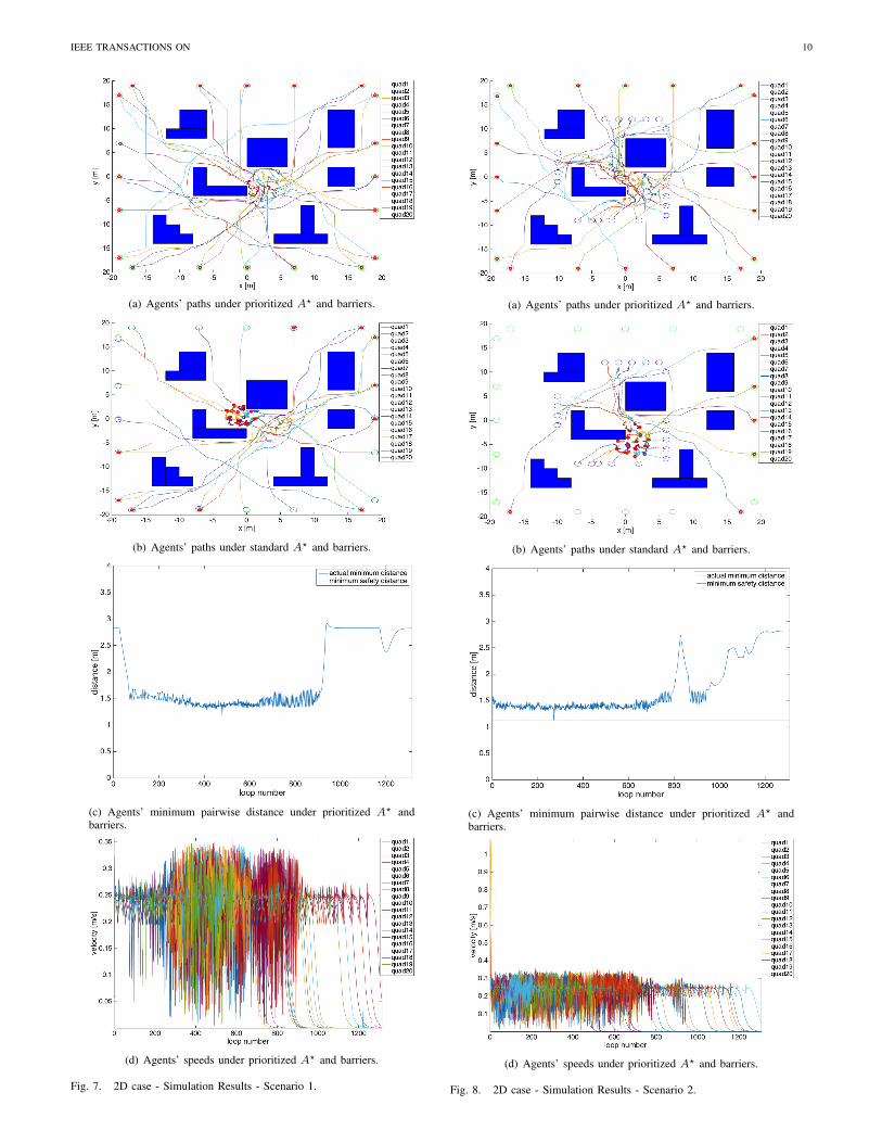
1) Scenario 1: The first scenario illustrates a case wherethe standard A? fails to find a safe and convergent pathfor each agent when they happen to operate in a highlycongested confined area, whereas the prioritized A? succeedsin generating both safe and convergent paths. The results areshown in Fig. 7.

The initial locations of the agents are such that the agentsare disconnected, while their final locations are such that thestraight-line paths intersect in the area around the centroidof the considered workspace. Each agent computes a pathto its goal using the proposed prioritized A? algorithm andmoves towards it under the control laws (15), (19). Obviously,since the agents are initially disconnected, the prioritized A?

essentially behaves as the standard A? in the first run of the

algorithm and while there are no connected groups. The A?

paths guide the agents in the area close to the centroid ofthe considered workspace. Whenever agents become pairwiseconnected, the prioritized A? is triggered, as described in Sec-tion III. The paths resulting from the prioritized A? algorithmin combination with the low-level barrier control are shownin Fig. 7(a), while the resulting paths for the case when thestandard A? is used instead of the prioritized A? is shownin Fig. 7(b). The prioritized A? forces the connected agentsto pick paths in a sequential spirit that are not overlappingfor a short horizon ahead, which is dictated by the numbern of nodes of the paths of the agents of higher prioritythat are communicated to, and avoided by, the agents oflower priority. Hence conflicts are resolved along paths thatsuppress congestion, and the agents are driven to their goaldestinations. In comparison, the standard A? per connectedagent does not take into account the other agents or theirnodes, resulting hence in overlapping paths, and defers theconflict resolution to the low-level barrier control. This inturn results in chattering, hence longer, and for some agentsnon-convergent paths, as shown in Fig. 7(b). Safety under theprioritized A? is demonstrated through Fig. 7(c) that depictsthe minimum pairwise inter-agent distance among all pairs ofconnected agents over time, and verifies that it remains greaterthan the safe separation. Finally the resulting speeds for theagents are shown in Fig. 7(d), and are bounded as expectedby the definition of the low-level controller.

2) Scenario 2: The second scenario illustrates a case wherethe initial locations of the agents are such that a congestedarea, and in turn connected groups of agents, are formed inthe neighborhood of the centroid of the considered workspaceat initial time t = 0. These initial conditions trigger theprioritized A?. As shown in Fig. 8(a), the agents manage toresolve conflicts and converge to their goal destinations. Incontrast, the standard A? (in combination with the low-levelbarrier control) fails to find convergent paths for all agents,as illustrated in Fig. 8(b). Furthermore, inter-agent collisionsunder the prioritized A? are avoided as demonstrated by theminimum pairwise distance illustrated in Fig. 8(c), while theresulting speeds for the agents are shown in Fig. 8(d).

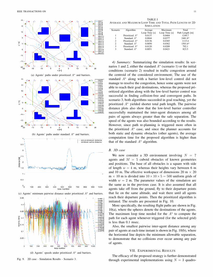
3) Scenario 3: The third scenario illustrates a case whereboth the prioritized A? and the standard A?, combined asalways with the barrier control, succeed in finding safe andconvergent paths, yet the prioritized A? results in shortertraveled paths. The results of this simulation are shown inFig. 9. The agents’ initial and final locations in this case arechosen such that no areas of high congestion are formed; as aresult, both the prioritized and the standard A? along with thebarriers find collision-free and convergent paths. Nevertheless,the total path length in the former case is shorter than in thelatter case, see Table I.

Table I in addition provides the average and maximum looptime for the prioritized and the standard A?, respectively, aswell as the total path length traveled by the agents in thepresented three scenarios. Note that the values of the totallength marked by ”*” refer to the cases where not all agentsreached their goals, and the simulation was forced to stop afterrunning for a sufficiently long time.


(a) Agents’ paths under prioritized A? and barriers.

(b) Agents’ paths under standard A? and barriers.

(c) Agents’ minimum pairwise distance under prioritized A? andbarriers.

(d) Agents’ speeds under prioritized A? and barriers.

Fig. 7. 2D case - Simulation Results - Scenario 1.



(c) Agents’ minimum pairwise distance under prioritized A? andbarriers.






(c) Agents’ minimum pairwise distance under prioritized A? and barriers.



TABLE IAVERAGE AND MAXIMUM LOOP TIME AND TOTAL PATH LENGTH OF 2D

SIMULATION

Scenario Algorithm Average Maximum TotalLoop Time [s] Loop Time [s] Path Length [m]

1 Prioritized A? 0.0137 0.0404 1249.71 Standard A? 0.0044 0.0377 2481.8*2 Prioritized A? 0.0136 0.0385 1115.42 Standard A? 0.0050 0.0362 1501.6*3 Prioritized A? 0.0120 0.0289 792.13 Standard A? 0.0051 0.0421 823.5

4) Summary: Summarizing the simulation results: In sce-narios 1 and 2, either the standard A? (scenario 1) or the initialconditions (scenario 2) resulted in traffic congestion aroundthe centroid of the considered environment; The use of thestandard A? along with a barrier low-level control did notmanage to resolve the congestion, hence some agents were notable to reach their goal destinations, whereas the proposed pri-oritized algorithm along with the low-level barrier control wassuccessful in finding collision-free and convergent paths. Inscenario 3, both algorithms succeeded in goal reaching, yet theprioritized A? yielded shorter total path length. The pairwisedistance plots also show that the low-level barrier controllersuccessfully maintained the inter-agent distances among allpairs of agents always greater than the safe separation. Thespeed of the agents was also bounded according to the results.However, since path re-planning is triggered more often inthe prioritized A? case, and since the planner accounts forboth static and dynamic obstacles (other agents), the averagecomputation time for the proposed algorithm is higher thanthat of the standard A? algorithm.

B. 3D case

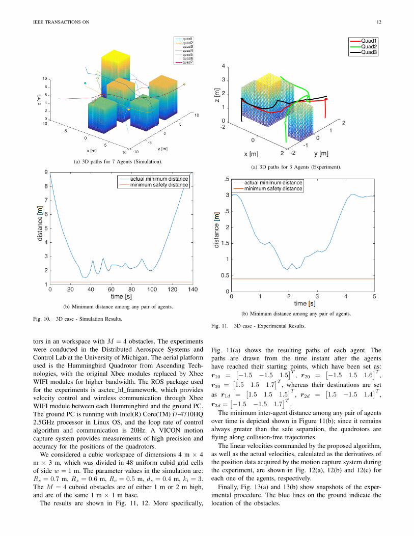
We now consider a 3D environment involving N = 7agents and M = 5 cuboid obstacles of known geometriesand positions. The base of all obstacles is a square with sideof length w = 4 m, whereas their heights vary between 6 mand 10 m. The effective workspace of dimensions 20 m × 20m × 10 m is divided into 10× 10× 5 = 500 uniform grids ofwidth w = 2 m. The parameter values of the simulation arethe same as in the previous case. It is also assumed that allagents take off from the ground, fly to their departure pointsthat lie on the same altitude, and wait there until all agentsreach their departure points. Then the prioritized algorithm isinitiated. The results are presented in Fig. 10.

More specifically, the resulting flight paths are shown in Fig.10(a), where the spheres denote the destinations of the agents.The maximum loop time needed for the A? to compute thepath for each agent whenever triggered (for the selected grid)is less than 0.1 msec.

Also, the smallest pairwise inter-agent distance among anypair of agents at each time instant is shown in Fig. 10(b), wherethe horizontal line depicts the minimum allowable separation,to demonstrate that no collisions ever occur among any pairof agents.

VII. EXPERIMENTAL RESULTS

The efficacy of the proposed strategy is further demonstratedthrough experimental implementations using N = 3 quadro-


(a) 3D paths for 7 Agents (Simulation).

(b) Minimum distance among any pair of agents.

Fig. 10. 3D case - Simulation Results.

tors in an workspace with M = 4 obstacles. The experimentswere conducted in the Distributed Aerospace Systems andControl Lab at the University of Michigan. The aerial platformused is the Hummingbird Quadrotor from Ascending Tech-nologies, with the original Xbee modules replaced by XbeeWIFI modules for higher bandwidth. The ROS package usedfor the experiments is asctec hl framework, which providesvelocity control and wireless communication through XbeeWIFI module between each Hummingbird and the ground PC.The ground PC is running with Intel(R) Core(TM) i7-4710HQ2.5GHz processor in Linux OS, and the loop rate of controlalgorithm and communication is 20Hz. A VICON motioncapture system provides measurements of high precision andaccuracy for the positions of the quadrotors.

We considered a cubic workspace of dimensions 4 m × 4m × 3 m, which was divided in 48 uniform cubid grid cellsof side w = 1 m. The parameter values in the simulation are:Rs = 0.7 m, Rz = 0.6 m, Rc = 0.5 m, ds = 0.4 m, ki = 3.The M = 4 cuboid obstacles are of either 1 m or 2 m high,and are of the same 1 m × 1 m base.

The results are shown in Fig. 11, 12. More specifically,

(a) 3D paths for 3 Agents (Experiment).

(b) Minimum distance among any pair of agents.

Fig. 11. 3D case - Experimental Results.

Fig. 11(a) shows the resulting paths of each agent. Thepaths are drawn from the time instant after the agentshave reached their starting points, which have been set as:r10 =

[−1.5 −1.5 1.5

]T, r20 =

[−1.5 1.5 1.6

]T,

r30 =[1.5 1.5 1.7

]T, whereas their destinations are set

as r1d =[1.5 1.5 1.5

]T, r2d =

[1.5 −1.5 1.4

]T,

r3d =[−1.5 −1.5 1.7

]T.

The minimum inter-agent distance among any pair of agentsover time is depicted shown in Figure 11(b); since it remainsalways greater than the safe separation, the quadrotors areflying along collision-free trajectories.

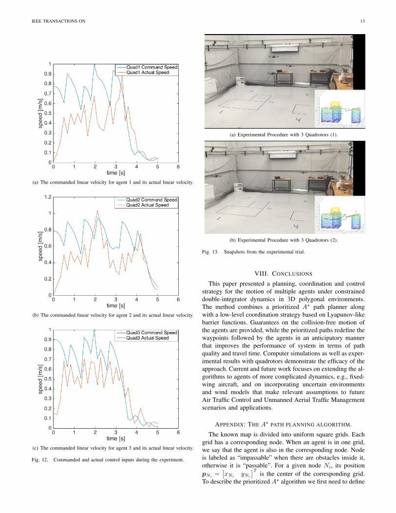
The linear velocities commanded by the proposed algorithm,as well as the actual velocities, calculated as the derivatives ofthe position data acquired by the motion capture system duringthe experiment, are shown in Fig. 12(a), 12(b) and 12(c) foreach one of the agents, respectively.

Finally, Fig. 13(a) and 13(b) show snapshots of the exper-imental procedure. The blue lines on the ground indicate thelocation of the obstacles.


(a) The commanded linear velocity for agent 1 and its actual linear velocity.

(b) The commanded linear velocity for agent 2 and its actual linear velocity.

(c) The commanded linear velocity for agent 3 and its actual linear velocity.

Fig. 12. Commanded and actual control inputs during the experiment.

(a) Experimental Procedure with 3 Quadrotors (1).

(b) Experimental Procedure with 3 Quadrotors (2).

Fig. 13. Snapshots from the experimental trial.

VIII. CONCLUSIONS

This paper presented a planning, coordination and controlstrategy for the motion of multiple agents under constraineddouble-integrator dynamics in 3D polygonal environments.The method combines a prioritized A? path planner alongwith a low-level coordination strategy based on Lyapunov-likebarrier functions. Guarantees on the collision-free motion ofthe agents are provided, while the prioritized paths redefine thewaypoints followed by the agents in an anticipatory mannerthat improves the performance of system in terms of pathquality and travel time. Computer simulations as well as exper-imental results with quadrotors demonstrate the efficacy of theapproach. Current and future work focuses on extending the al-gorithms to agents of more complicated dynamics, e.g., fixed-wing aircraft, and on incorporating uncertain environmentsand wind models that make relevant assumptions to futureAir Traffic Control and Unmanned Aerial Traffic Managementscenarios and applications.

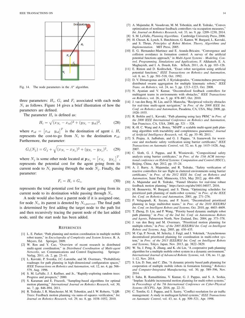
APPENDIX: THE A? PATH PLANNING ALGORITHM.

The known map is divided into uniform square grids. Eachgrid has a corresponding node. When an agent is in one grid,we say that the agent is also in the corresponding node. Nodeis labeled as “impassable” when there are obstacles inside it,otherwise it is “passable”. For a given node Ni, its positionpNi

=[xNi

yNi

]Tis the center of the corresponding grid.

To describe the prioritized A? algorithm we first need to define


Fig. 14. The node parameters in the A? algorithm.

three parameters: Hi, Gi and Fi associated with each nodeNi as follows. Figure 14 gives a brief illustration of how theparameters are defined.

The parameter Hi is defined as:

Hi =√

(xNi − xid)2 + (yNi − yid)2, (28)

where rid =[xid yid

]Tis the destination of agent i. Hi

represents the cost-to-go from Ni to the destination rid.Furthermore, the parameter:

Gi(Nj) = Gj +√

(xNi− xNj

)2 + (yNi− yNj

)2, (29)

where Nj is some other node located at pNj =[xNj

yNj

]T,

represents the potential cost for the agent going from itscurrent node to Ni passing through the node Nj . Finally, theparameter:

Fi = Hi +Gi, (30)

represents the total potential cost for the agent going from itscurrent node to its destination while passing through Ni.

A node would also have a parent node if it is assigned one,for node Ni, its parent is denoted by Ni,parent. The final pathis determined by first adding the target node to the path listand then recursively tracing the parent node of the last addednode, until the start node has been added.

REFERENCES

[1] L. E. Parker, “Path planning and motion coordination in multiple mobilerobot teams,” in Encyclopedia of Complexity and System Science, R. A.Meyers, Ed. Springer, 2009.

[2] W. Ren and Y. Cao, “Overview of recent research in distributedmulti-agent coordination,” in Distributed Coordination of Multi-agentNetworks, ser. Communications and Control Engineering. Springer-Verlag, 2011, ch. 2, pp. 23–41.

[3] L. Kavraki, P. Svestka, J.C.-Latombe, and M. Overmars, “Probabilisticroadmaps for path planning in high-dimensional configuration spaces,”IEEE Transactions on Robotics and Automation, vol. 12, no. 4, pp. 566–579, Aug. 1996.

[4] S. M. LaValle, J. J. Kuffner, and Jr., “Rapidly-exploring random trees:Progress and prospects,” 2000.

[5] S. Karaman and E. Frazzoli, “Sampling-based algorithms for optimalmotion planning,” International Journal on Robotics Research, vol. 30,no. 7, pp. 846–894, 2011.

[6] R. Tedrake, I. R. Manchester, M. M. Tobenkin, and J. W. Roberts, “LQR-Trees: Feedback motion planning via sums-of-squares verification,” Int.Journal on Robotics Research, vol. 29, no. 8, pp. 1038–1052, 2010.

[7] A. Majumdar, R. Vasudevan, M. M. Tobenkin, and R. Tedrake, “Convexoptimization of nonlinear feedback controllers via occupation measures,”Int. Journal on Robotics Research, vol. 33, no. 9, pp. 1209–1230, 2014.

[8] S. M. LaValle, Planning Algorithms. Cambridge University Press, 2006.[9] H. Choset, K. Lynch, S. Hutchinson, G. Kantor, W. Burgard, L. Kavraki,

and S. Thrun, Principles of Robot Motion. Theory, Algorithms andImplementation. MIT Press, 2005.

[10] E. G. Hernandez-Martinez and E. Aranda-Bricaire, “Convergence andcollision avoidance in formation control: A survey of the artificialpotential functions approach,” in Multi-Agent Systems - Modeling, Con-trol, Programming, Simulations and Applications, F. Alkhateeb, E. A.Maghayreh, and I. A. Doush, Eds. InTech, 2011, ch. 6, pp. 103–126.

[11] E. Rimon and D. Koditschek, “Exact robot navigation using artificialpotential functions,” IEEE Transactions on Robotics and Automation,vol. 8, no. 5, pp. 501–518, Oct. 1992.

[12] D. V. Dimarogonas and K. J. Kyriakopoulos, “Connectedness preservingdistributed swarm aggregation for multiple kinematic robots,” IEEETrans. on Robotics, vol. 24, no. 5, pp. 1213–1223, Oct. 2008.

[13] N. Ayanian and V. Kumar, “Decentralized feedback controllers formultiagent teams in environments with obstacles,” IEEE Transactionson Robotics, vol. 26, no. 5, pp. 878–887, Oct. 2010.

[14] J. van den Berg, M. Lin, and D. Manocha, “Reciprocal velocity obstaclesfor real-time multi-agent navigation,” in Proc. of the 2008 IEEE Int.Conf. on Robotics and Automation, Pasadena, CA, USA, May 2008, pp.1928–1935.

[15] R. Bohlin and L. Kavraki, “Path planning using lazy PRM,” in Proc. ofthe 2000 IEEE International Conference on Robotics and Automation,San Francisco, CA, USA, 2000, pp. 521 – 528.

[16] K.-H. C. Wang and A. Botea, “MAPP: a scalable multi-agent path plan-ning algorithm with tractability and completeness guarantees,” Journalof Artificial Intelligence Research, vol. 42, pp. 55–90, 2011.

[17] S. Prajna, A. Jadbabaie, and G. J. Pappas, “A framework for worst-case and stochastic safety verification using barrier certificates,” IEEETransactions on Automatic Control, vol. 52, no. 8, pp. 1415–1428, Aug.2007.

[18] C. Sloth, G. J. Pappas, and R. Wisniewski, “Compositional safetyanalysis using barrier certificates,” in Proc. of the 15th ACM interna-tional conference on Hybrid Systems: Computation and Control (HSCC),Beijing, China, Apr. 2012, pp. 15–24.

[19] A. J. Barry, A. Majumdar, and R. Tedrake, “Safety verification ofreactive controllers for uav flight in cluttered environments using barriercertificates,” in Proc. of the 2012 IEEE Int. Conf. on Robotics andAutomation, Saint Paul, Minnesota, USA, May 2012, pp. 484–490.

[20] A. Majumdar and R. Tedrake, “Funnel libraries for real-time robustfeedback motion planning,” https://arxiv.org/abs/1601.04037, 2016.

[21] M. Bennewitz, W. Burgard, and S. Thrun, “Optimizing schedules forprioritized path planning of multi-robot systems,” in Proc. of the IEEEInt. Conf. on Robotics and Automation, 2001, pp. 271–276.

[22] P. Velagapudi, K. Sycara, and P. Scerri, “Decentralized prioritizedplanning in large multirobot teams,” in Proc. of the 2010 IEEE/RSJInt. Conf. on Intelligent Robots and Systems, Oct. 2010, pp. 4603–4609.

[23] T. Zheng, D. Liu, and P. Wang, “Priority based dynamic multiple robotpath planning,” in Proc. of the 2nd Int. Conf. on Autonomous Robotsand Agents, Palmerston North, New Zealand, Dec. 2004, pp. 373–378.

[24] J. van den Berg and M. Overmars, “Prioritized motion planning formultiple robots,” in Proc. of the 2005 IEEE/RSJ Int. Conf. on IntelligentRobots and Systems, Aug. 2005, pp. 430–435.

[25] M. Cap, P. Novak, M. Selecky, J. Faigl, and J. Vokrinek, “Asynchronousdecentralized prioritized planning for coordination in multi-robot sys-tem,” in Proc. of the 2013 IEEE/RSJ Int. Conf. on Intelligent Robotsand Systems, Tokyo, Japan, Nov. 2013, pp. 3822–3829.

[26] W. Yu, J. Peng, X. Zhang, and K. chi Lin, “A cooperative path planningalgorithm for a multiple mobile robot system in a dynamic environment,”International Journal of Advanced Robotic Systems, vol. 136, no. 11, pp.1–12, Nov. 2014.

[27] S. Liu, D. Sun, and C. Zhu, “A dynamic priority based path planning forcooperation of multiple mobile robots in formation forming,” Roboticsand Computer-Integrated Manufacturing, vol. 30, pp. 589–596, Nov.2014.

[28] I. Saha, R. Ramaithitima, V. Kumar, G. J. Pappas, and S. A. Seshia,“Implan: Scalable incremental motion planning for multi-robot systems,”in Proceedings of the 7th International Conference on Cyber-PhysicalSystems (ICCPS), Apr. 2016, pp. 22–31.

[29] C. Tomlin, G. J. Pappas, and S. Sastry, “Conflict resolution for air trafficmanagement: A study in multiagent hybrid systems,” IEEE Transactionson Automatic Control, vol. 43, no. 4, pp. 509–521, Apr. 1998.


[30] K. Zeghal, “A review of different approaches based on force fields forairborne conflict resolution,” in AIAA Guidance, Navigation, and ControlConference, Boston, Aug. 1998, pp. AIAA Paper 1998–4240.

[31] E. Frazzoli, Z.-H. Mao, J.-H. Oh, and E. Feron, “Resolution of conflictsinvolving many aircraft via semidefinite programming,” Journal ofGuidance, Control and Dynamics, vol. 24, no. 1, pp. 179–189, Jan.2001.

[32] M. R. Jardin, “Analytical relationships between conflict counts and air-traffic density,” Journal of Guidance, Control and Dynamics, vol. 28,no. 6, pp. 1150–1156, Jan. 2005.

[33] G. Dowek, C. Munoz, and V. A. Carreno, “Provably safe coordinatedstrategy for distributed conflict resolution,” in AIAA Guidance, Navi-gation, and Control Conference and Exhibit, San Francisco, CA, Aug.2005, pp. AIAA–2005–6047.

[34] M. A. Christodoulou and S. G. Kodaxakis, “Automatic commercialaircraft-collision avoidance in free flight: The three-dimensional prob-lem,” IEEE Transactions on Intelligent Transportation Systems, vol. 7,no. 2, pp. 242–249, June 2006.

[35] A. L. Galdino, C. M. noz, and M. Ayala-Rincon, “Formal verificationof an optimal air traffic conflict resolution and recovery algorithm,” inLogic, Language, Information and Computation, ser. Lecture Notes inComputer Science. Berlin Heidelberg: Springer-Verlag, 2007, vol. 4576,pp. 177–188.

[36] M. Gariel and E. Feron, “Graceful degradation of air traffic operations:Airspace sensitivity to degraded surveillance systems,” Proceedings ofthe IEEE, vol. 96, no. 12, pp. 2028–2039, Dec. 2008.

[37] A. Platzer, “Air traffic collision avoidance,” in Logical Analysis ofHybrid Systems. Berlin Heidelberg: Springer-Verlag, 2010, pp. 303–334.

[38] A. Alonso-Ayuso, L. F. Escudero, and F. J. Martın-Campo, “Collisionavoidance in air traffic management: A mixed-integer linear optimizationapproach,” IEEE Transactions on Intelligent Transportation Systems,vol. 12, no. 1, pp. 47–57, Mar. 2011.

[39] J. Le Ny and G. J. Pappas, “Joint metering and conflict resolution in airtraffic control,” Journal of Guidance, Control and Dynamics, vol. 34,no. 5, pp. 475–482, Sept. 2011.

[40] M. J. Kochenderfer, J. E. Holland, and J. P. Chryssanthacopoulos, “Next-generation airborne collision avoidance system,” Lincoln LaboratoryJournal, vol. 19, no. 1, pp. 17–33, 2012.

[41] J.-B. Jeannin, K. Ghorbal, Y. Kouskoulas, R. Gardner, A. Schmidt,E. Zawadzki, and A. Platzer, “A formally verified hybrid system forthe next-generation airborne collision avoidance system,” in Tools andAlgorithms for the Construction and Analysis of Systems, 2015, pp. 21–36.

[42] D. Panagou, D. M. Stipanovic, and P. G. Voulgaris, “Distributed coordi-nation and control of multi-robot networks using Lyapunov-like barrierfunctions,” IEEE Transactions on Automatic Control, vol. 61, no. 3, pp.617–632, Mar. 2016.

[43] D. Panagou, “A distributed feedback motion planning protocol formultiple unicycle agents of different classes,” IEEE Transactions onAutomatic Control, pp. accepted as Full Paper, to appear., 2016.

[44] X. Ma, Z. Jiao, Z. Wang, and D. Panagou, “Decentralized prioritizedmotion planning for multiple autonomous UAVs in 3d polygonal obsta-cle environments,” in Proc. of the 2016 Int. Conf. on Unmanned AircraftSystems (ICUAS), Arlington, VA, USA, June 2016, pp. 292–300.

[45] A. G. Wills and W. P. Heath, “A recentred barrier for constrainedreceding horizon control,” in Proc. of the American Control Conference,Anchorage, AK, USA, May 2002, pp. 4177–4182.

Xiaobai Ma was born in Weinan, Shaanxi, China,in 1993. He received the B.S.E degree in AerospaceEngineering from University of Michigan, Michigan,United States, in 2016, and the B.E degree in Electri-cal and Computer Engineering from Shanghai JiaoTong University, Shanghai, China, in 2016. He iscurrently a first year Master student in the depart-ment of Aeronautics and Astronautics at StanfordUniversity. His current research interests includedeep reinforcement learning and autonomous driv-ing.

Ziyuan Jiao was born in Beijing, China, in 1993. Hereceived the B.S.E degree in Aerospace Engineer-ing from University of Michigan, Michigan, UnitedStates, in 2016, and the B.E degree in MechanicalEngineering from Shanghai Jiao Tong University,Shanghai, China, in 2016. He is currently a Masterstudent in the department of Mechanical Engineer-ing, University of Michigan. His current researchinterests include dynamics and control in roboticssystems, mechatronic system design and control inmanufacturing.

Zhenkai Wang is a graduate student of Aeronauticsand Astronautics at Stanford University. He earnedhis B.S.E. in Aerospace Engineering from Universityof Michigan, Ann Arbor, in 2016, and then B.S.E.in Electrical and Computer Engineering at ShanghaiJiao Tong University, in the same year. His researchinterests include motion planning, computer visionand robotic perception.

Dimitra Panagou received the Diploma and PhDdegrees in Mechanical Engineering from the Na-tional Technical University of Athens, Greece, in2006 and 2012, respectively. Since September 2014she has been an Assistant Professor with the De-partment of Aerospace Engineering, University ofMichigan. Prior to joining the University of Michi-gan, Dr. Panagou was a postdoctoral research as-sociate with the Coordinated Science Laboratory,University of Illinois, Urbana-Champaign (2012-2014), a visiting research scholar with the GRASP

Lab, University of Pennsylvania (June 2013, fall 2010) and a visiting researchscholar with the University of Delaware, Mechanical Engineering Depart-ment (spring 2009). Her research interests include the fields of planning,coordination and distributed control of complex systems, with applicationsin unmanned aerial systems, robotic networks and autonomous multi-vehiclesystems (ground, marine, aerial, space). She is a recipient of a NASA EarlyFaculty Career Award, of an AFOSR Young Investigator Award, and memberof the IEEE and the AIAA.

Documents

IEEE TRANSACTIONS ON 1 3D Decentralized Prioritized Motion ...dpanagou/assets/documents/XMa_TCST… · 3D Decentralized Prioritized Motion Planning and Coordination for High-Density