Embed Size (px)
Citation preview

Chapter �
Parabolic Problems
��� Introduction
The �nite element method may be used to solve time�dependent problems as well as
steady ones� This e�ort involves both parabolic and hyperbolic partial di�erential sys�
tems� Problems of parabolic type involve di�usion and dissipation while hyperbolic
problems are characterized by conservation of energy and wave propagation� Simple
one�dimensional heat conduction and wave propagation equations will serve as model
problems of each type�
Example ������ The one�dimensional heat conduction equation
ut � puxx� a � x � b� t � �� ������a
where p is a positive constant called the di�usivity is of parabolic type� Initial�boundary
value problems consist of determining u�x� t satisfying ������a given the initial data
u�x� � � u��x� a � x � b� ������b
and appropriate boundary data e�g�
pux�a� t � ��u�a� t � ���t� pux�b� t � ��u�b� t � ���t� ������c
As with elliptic problems boundary conditions without the pux term are called Dirichlet
conditions� those with �i � � i � �� � are Neumann conditions� and those with both
terms present are called Robin conditions� The problem domain is open in the time
direction t� thus unlike elliptic systems this problem is evolutionary and computation
continues in t for as long as there is interest in the solution�
Example ������ The one�dimensional wave equation
utt � c�uxx� a � x � b� t � �� ����� a
�

Parabolic Problems
where c is a constant called the wave speed is a hyperbolic partial di�erential equation�
Initial�boundary value problems consist of determining u�x� t satisfying ����� a given
the initial data
u�x� � � u��x� ut�x� � � �u��x� a � x � b� ����� b
and boundary data of the form ������c� Small transverse vibrations of a taut string
satisfy the wave equation� In this case u�x� t is the transverse displacement of the
string and c� � T�� T being the applied tension and � being the density of the string�
We�ll study parabolic problems in this chapter and hyperbolic problems in the next�
We shall see that there are two basic �nite element approaches to solving time�dependent
problems� The �rst called the method of lines uses �nite elements in space and ordinary
di�erential equations software in time� The second uses �nite element methods in both
space and time� We�ll examine the method of lines approach �rst and then tackle space�
time �nite element methods�
��� Semi�Discrete Galerkin Problems� The Method
of Lines
Let us consider a parabolic problem of the form
ut � L�u� � f�x� y� �x� y � �� t � �� ��� ��a
where L is a second�order elliptic operator� In two dimensions u would be a function of
x y and t and L�u� could be the very familiar
L�u� � ��puxx � �puyy � qu� ��� ��b
Appropriate initial and boundary conditions would also be needed e�g�
u�x� y� � � u��x� y� �x� y � � � ��� ��� ��c
u�x� y� t � �x� y� t� �x� y � ��E � ��� ��d
pun � �u � �� �x� y � ��N � ��� ��e
We construct a Galerkin formulation of ��� �� in space in the usual manner� thus we
multiply ��� ��a by a suitable test function v and integrate the result over � to obtain
�v� ut � �v�L�u� � �v� f�

���� Semi�Discrete Galerkin Problems �
As usual we apply the divergence theorem to the second�derivative terms in L to reduce
the continuity requirements on u� When L has the form of ��� ��b the Galerkin problem
consists of determining u � H�E � �t � � such that
�v� ut � A�v� u � �v� f� � v� � � �u �� �v � H�� � t � �� ��� � a
The L� inner product strain energy and boundary inner product are as with elliptic
problems
�v� f �
ZZ�
vfdxdy� ��� � b
A�v� u �
ZZ�
�p�vxux � vyuy � vqu�dxdy� ��� � c
and
� v� pun ��
Z��N
vpunds� ��� � d
The natural boundary condition ��� ��e has been used to replace pun in the boundary
inner product� Except for the presence of the �v� ut term the formulation appears to
the same as for an elliptic problem�
Initial conditions for ��� � a are usually determined by projection of the initial data
��� ��c either in L�
�v� u � �v� u�� �v � H�� � t � �� ��� ��a
or in strain energy
A�v� u � A�v� u�� �v � H�� � t � �� ��� ��b
Example ������ We analyze the one�dimensional heat conduction problem
ut � �puxx � f�x� t� � � x � �� t � ��
u�x� � � u��x� � � x � ��
u��� t � u��� t � �� t � ��
thoroughly in the spirit that we did in Chapter � for a two�point boundary value problem�
A Galerkin form of this heat�conduction problem consists of determining u � H��
satisfying
�v� ut � A�v� u � �v� f� �v � H�� � t � ��

� Parabolic Problems
x
0 = x x x x
U(x,t)
0 N-1 N1 jx = 1
c
c
c
j
1N-1
Figure �� ��� Mesh for the �nite element solution of Example �� ���
�v� u � �v� u�� �v � H�� � t � ��
where
A�v� u �
Z �
�
vxpuxdx�
Boundary terms of the form ��� � d disappear because v � � at x � �� � with Dirichlet
data�
We introduce a mesh on � � x � � as shown in Figure �� �� and choose an approxi�
mation U of u in a �nite�dimensional subspace SN� of H�
� having the form
U�x� t �N��Xj��
cj�tj�x�
Unlike steady problems the coe�cients cj j � �� � � � � � N�� depend on t� The Galerkin
�nite element problem is to determine U � SN� such that
�j� Ut � A�j� U � �j� f� t � ��
�j� U � �j� u�� t � �� j � �� � � � � � N � ��
Let us chose a piecewise�linear polynomial basis
k�x �
�����
x�xk��xk�xk��
� if xk�� � x � xkxk���x
xk���xk� if xk � x � xk��
�� otherwise
�
This problem is very similar to the one�dimensional elliptic problem considered in Section
��� so we�ll skip several steps and also construct the discrete equations by vertices rather
than by elements�

���� Semi�Discrete Galerkin Problems �
Since j has support on the two elements containing node j we have
A�j� U �
Z xj
xj��
�jpUxdx�
Z xj��
xj
�jpUxdx
where � � � d� �dx� Substituting for j and Ux
A�j� U �
Z xj
xj��
�
hjp�x�
cj � cj��hj
dx�
Z xj��
xj
� �
hj��p�x�
cj�� � cjhj��
dx
where
hj � xj � xj���
Using the midpoint rule to evaluate the integrals we have
A�j� U � pj����hj
�cj � cj���pj����hj��
�cj�� � cj
where pj���� � p�xj�����
Similarly
�j� Ut �
Z xj
xj��
jUtdx�
Z xj��
xj
jUtdx
or
�j� Ut �
Z xj
xj��
j� �cj��j�� � �cjjdx�
Z xj��
xj
j� �cjj � �cj��j��dx
where �� � d� �dt� Since the integrands are quadratic functions of x they may be
integrated exactly using Simpson�s rule to yield
�j� Ut �hj�� �cj�� � �cj �
hj���
� �cj � �cj���
Finally
�j� f �Z xj
xj��
jf�xdx �
Z xj��
xj
jf�xdx�
Although integration of order one would do we�ll once again use Simpson�s rule to
obtain
�j� f � hj�� fj���� � fj �
hj���
�fj � fj�����
We could replace fj���� by the average of fj�� and fj to obtain a similar formula to the
one obtained for �j� Ut� thus
�j� f � hj��fj�� � fj �
hj���
� fj � fj���
Combining these results yields the discrete �nite element system
hj�� �cj�� � �cj �
hj���
� �cj � �cj�� �pj����hj
�cj � cj���pj����
hj � �� �cj�� � cj

� Parabolic Problems
�hj��fj�� � fj �
hj���
� fj � fj��� j � �� � � � � � N � ��
�We have dropped the � and written the equation as an equality�
If p is constant and the mesh spacing h is uniform we obtain
h
�� �cj�� � ��cj � �cj��� p
h�cj�� � cj � cj�� �
h
��fj�� � �fj � fj���
j � �� � � � � � N � ��
The discrete systems may be written in matrix form and for simplicity we�ll do so for
the constant coe�cient uniform mesh case to obtain
M �c�Kc � l ��� ��a
where
M �h
�
�������
� �� � �
� � � � � � � � �
� � �� �
������ � ��� ��b
K �p
h
�������
���� ��
� � � � � � � � �
�� ����
������ � ��� ��c
l �h
�
�����
f� � �f� � f�f� � �f� � f�
���fN�� � �fN�� � fN
���� � ��� ��d
c � �c�� c�� � � � � cN���T � ��� ��e
The matricesM K and l are the global mass matrix the global sti�ness matrix and
the global load vector� Actually M has little to do with mass and should more correctly
be called a global dissipation matrix� however we�ll stay with our prior terminology�
In practical problems element�by�element assembly should be used to construct global
matrices and vectors and not the nodal approach used here�
The discrete �nite element system ��� �� is an implicit system of ordinary di�erential
equations for �c� The mass matrix M can be �lumped� by a variety of tricks to yield an

���� Semi�Discrete Galerkin Problems �
explicit ordinary di�erential system� One such trick is to approximate �j� Ut by using
the right�rectangular rule on each element to obtain
�j� Ut �
Z xj
xj��
j� �cj��j�� � �cjjdx�
Z xj��
xj
j� �cjj � �cj��j��dx � hcj�
The resulting �nite element system would be
hI �c�Kc � l�
Recall �cf� Section ��� that a one�point quadrature rule is satisfactory for the conver�
gence of a piecewise�linear polynomial �nite element solution�
With the initial data determined by L� projection onto SNE we have
�j� U��� � � �j� u�� j � �� � � � � � N � ��
Numerical integration will typically be needed to evaluate �j� u� and we�ll approximate
it in the manner used for the loading term �j� f� Thus with uniform spacing we have
Mc�� � u� �h
�
�����
u�� � �u�� � u��u�� � �u�� � u��
���u�N�� � �u�N�� � u�N
���� � ��� ��f
If the initial data is consistent with the trivial Dirichlet boundary data i�e� if u� � H��
then the above system reduces to
cj�� � u��xj� j � �� � �� � � � � N � ��
Had we solved the wave equation ����� instead of the heat equation ������ using a
piecewise�linear �nite element basis we would have found the discrete system
M�c �Kc � � ��� ��
with p in ��� ��c replaced by c��
The resulting initial value problems �IVPs for the ordinary di�erential equations
�ODEs ��� ��a or ��� �� typically have to be integrated numerically� There are several
excellent software packages for solving IVPs for ODEs� When such ODE software is used
with a �nite element or �nite di�erence spatial discretization the resulting procedure is
called the method of lines� Thus the nodes of the �nite elements appear to be �lines�
in the time direction and as shown in Figure �� � for a one�dimensional problem the
temporal integration proceeds along these lines�

� Parabolic Problems
x
0 = x x x x0 N-1 N1 j
x = 1
t
Figure �� � � �Lines� for a method of lines integration of a one�dimensional problem�
Using the ODE software solutions are calculated in a series of time steps ��� t��
�t�� t�� � � � � Methods fall into two types� Those that only require knowledge of the so�
lution at time tn in order to obtain a solution at time tn�� are called one�step methods�
Correspondingly methods that require information about the solution at tn and several
times prior to tn are calledmultistep methods� Excellent texts on the subject are available
� � � ��� One�step methods are Runge�Kutta methods while the common multistep
methods are Adams or backward di�erence methods� Software based on these methods
automatically adjusts the time steps and may also automatically vary the order of accu�
racy of a class of methods in order to satisfy a prescribed local error tolerance minimize
computational cost and maintain numerical e�ciency�
The choice of a one�step or multistep method will depend on several factors� Gener�
ally Runge�Kutta methods are preferred when time integration is simple relative to the
spatial solution� Multistep methods become more e�cient for complex nonlinear prob�
lems� Implicit Runge�Kutta methods may be e�cient for problems with high�frequency
oscillations� The ODEs that arise from the �nite element discretization of parabolic
problems are �sti�� � �� so backward di�erence methods are the preferred multistep
methods�
Most ODE software � � �� addresses �rst�order IVPs of the explicit form
�y�t � f�t�y�t� y�� � y�� ��� ��
Second�order systems such as ��� �� would have to be written as a �rst�order system by
e�g� letting
d � �c

���� Semi�Discrete Galerkin Problems �
and hence obtaining �c
M �d
��
d
�Kc��
Unfortunately systems having the form of ��� ��a or the one above are implicit and
would require inverting or lumping M in order to put them into the standard explicit
form ��� ��� Inverting M is not terribly di�cult when M is constant or independent
of t� however it would be ine�cient for nonlinear problems and impossible when M is
singular� The latter case can occur when e�g� a heat conduction and a potential problem
are solved simultaneously�
Codes for di�erential�algebraic equations �DAEs directly address the solution of im�
plicit systems of the form
f�t�y�t� �y�t � �� y�� � y�� ��� ��
One of the best of these is the code DASSL written by Petzold ���� DASSL uses variable�
step variable�order backward di�erence methods to solve problems without needingM��
to exist�
Let us illustrate these concepts by applying some simple one�step schemes to problems
having the forms ��� �� or ��� ��� However implementation of these simple methods
is only justi�ed in certain special circumstances� In most cases it is far better to use
existing ODE software in a method of lines framework�
For simplicity we�ll assume that all boundary data is homogeneous so that the bound�
ary inner product in ��� � a vanishes� Selecting a �nite�dimensional space SN� � H�
� we
then determine U as the solution of
�V� Ut � A�V� U � �V� f� �v � SN� � ��� ��
Evaluation leads to ODEs having the form of ��� ��a regardless of whether or not the
system is one�dimensional or the coe�cients are constant� The actual matricesM and K
and load vector l will of course di�er from those of Example �� �� in these cases� The
systems ��� ��a or ��� �� are called semi�discrete Galerkin equations because time has
not yet been discretized�
We discretize time into a sequence of time slices �tn� tn��� of duration �t with tn �
n�t n � �� �� � � � � For this discussion no generality is lost by considering uniform time
steps� Let�
u�x� tn be the exact solution of the Galerkin problem ��� � a at t � tn�
U�x� tn be the exact solution of the semi�discrete Galerkin problem ��� �� at t � tn�
Un�x be the approximation of U�x� tn obtained by ODE software�

�� Parabolic Problems
cj�tn be the Galerkin coe�cient at t � tn� thus for a one�dimensional problem
U�x� tn �N��Xj��
cj�tnj�x�
For a Lagrangian basis cj�tn � U�xj � tn�
cnj be the approximation of cj�tn obtained by ODE software� For a one�dimensional
problem
Un�x �N��Xj��
cnj j�x�
We suppose that all solutions are known at time tn and that we seek to determine
them at time tn��� The simplest numerical scheme for doing this is the forward Euler
method where ��� �� is evaluated at time tn and
Ut�x� tn � Un���x� Un�x
�t� ��� ��
A simple Taylor�s series argument reveals that the local discretization error of such an
approximation is O��t� Substituting ��� �� into ��� �� yields
�V�Un�� � Un
�t � A�V� Un � �V� fn� �v � SN
� � ��� ���a
Evaluation of the inner products leads to
Mcn�� � cn
�t�Kncn � ln� ��� ���b
We have allowed the sti�ness matrix and load vector to be functions of time� The mass
matrix would always be independent of time for di�erential equations having the explicit
form of ��� ��a as long as the spatial �nite element mesh does not vary with time�
The ODEs ��� ���ab are implicit unless M is lumped� If lumping were used and e�g�
M � hI then cn�� would be determined as
cn�� � cn ��t
h�ln �Kncn��
Assuming that cn is known we can determine cn�� by inverting M�
Using the backward Euler method we evaluate ��� �� at tn�� and use the approxi�
mation ��� �� to obtain
�V�Un�� � Un
�t � A�V� Un�� � �V� fn��� �v � SN
� � ��� ���a
���� Semi�Discrete Galerkin Problems ��
and
Mcn�� � cn
�t�Kn��cn�� � ln��� ��� ���b
The backward Euler method is implicit regardless of whether or not lumping is used�
Computation of cn�� requires inversion of
�
�tM�Kn���
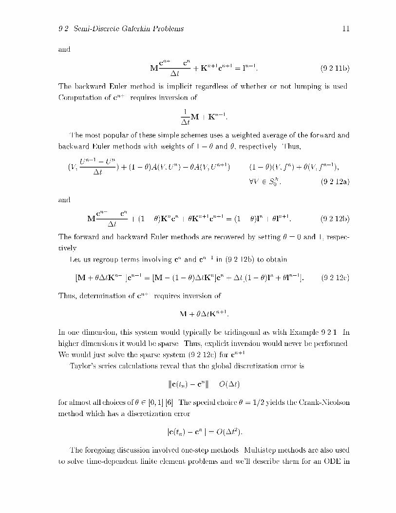
The most popular of these simple schemes uses a weighted average of the forward and
backward Euler methods with weights of �� � and � respectively� Thus
�V�Un�� � Un
�t � ��� �A�V� Un � �A�V� Un�� � ��� ��V� fn � ��V� fn���
�V � SN� � ��� �� a
and
Mcn�� � cn
�t� ��� �Kncn � �Kn��cn�� � ��� �ln � �ln��� ��� �� b
The forward and backward Euler methods are recovered by setting � � � and � respec�
tively�
Let us regroup terms involving cn and cn�� in ��� �� b to obtain
�M � ��tKn���cn�� � �M� ��� ��tKn�cn ��t���� �ln � �ln���� ��� �� c
Thus determination of cn�� requires inversion of
M � ��tKn���
In one dimension this system would typically be tridiagonal as with Example �� ��� In
higher dimensions it would be sparse� Thus explicit inversion would never be performed�
We would just solve the sparse system ��� �� c for cn���
Taylor�s series calculations reveal that the global discretization error is
kc�tn� cnk � O��t
for almost all choices of � � ��� �� ���� The special choice � � �� yields the Crank�Nicolson
method which has a discretization error
kc�tn� cnk � O��t��
The foregoing discussion involved one�step methods� Multistep methods are also used
to solve time�dependent �nite element problems and we�ll describe them for an ODE in

� Parabolic Problems
the implicit form ��� ��� The popular backward di�erence formulas �BDFs approximate
y�t in ��� �� by a k th degree polynomial Y�t that interpolates y at the k � � times
tn���i i � �� �� � � � � k� The derivative �y is approximated by �Y� The Newton backward
di�erence form of the interpolating is most frequently used to represent Y � �� but
since we�re more familiar with Lagrangian interpolation we�ll write
y�t � Y�t �kX
i��
yn���iNi�t� t � �tn���k� tn���� ��� ���a
where
Ni�t �kY
j���j ��i
t� tn���jtn���i � tn���j
� ��� ���b
The basis ��� ���b is represented by the usual Lagrangian shape functions �cf� Section
�� so Ni�tn���j � �ij�
Assuming yn���i i � �� � � � � � k to be known the unknown yn�� is determined by
collocation at tn��� Thus using ��� ��
f�tn���Y�tn��� �Y�tn�� � �� ��� ���
Example ������ The simplest BDF formula is obtained by setting k � � in ��� ��� to
obtain
Y�t � yn��N��t � ynN��t�
N��t �t� tn
tn�� � tn� N��t �
t� tn��tn � tn��
�
Di�erentiating Y�t
�Y�t �yn�� � yn
tn�� � tn�
thus the numerical method ��� ��� is the backward Euler method
f�tn���yn���
yn�� � yn
tn�� � tn � ��
Example ������ The second�order BDF follows by setting k � in ��� ��� to get
Y�t � yn��N��t � ynN��t � yn��N��t
N��t ��t� tn�t� tn��
�t�� N��t �
�t� tn���t� tn��
��t� �
N��t ��t� tn���t� tn
�t��
where time steps are of duration �t�

���� Finite Element Methods in Time ��
Di�erentiating and setting t � tn��
�N��tn�� ��
�t� �N��tn�� � �
�t� �N��tn�� �
�
�t�
Thus
�Y�tn�� ��yn�� � �yn � yn��
�t
and the second�order BDF is
f�tn���yn���
�yn�� � �yn � yn��
�t � ��
Applying this method to ��� ��a yields
M�cn�� � �cn � cn��
�t�Kn��cn�� � ln���
Thus computation of cn�� requires inversion of
M
��t�K�
Backward di�erence formulas through order six are available � � � � ���
��� Finite Element Methods in Time
It is of course possible to use the �nite element method in time� This can be done
on space�time triangular or quadrilateral elements for problems in one space dimension�
on hexahedra tetrahedra and prisms in two space dimensions� and on four�dimensional
parallelepipeds and prisms in three space dimensions� However for simplicity we�ll focus
on the time aspects of the space�time �nite element method by assuming that the spatial
discretization has already been performed� Thus we�ll consider an ODE system in the
form ��� ��a and construct a Galerkin problem in time by multiplying it by a test
function w � L� and integrating on �tn� tn��� to obtain
�w�M �cn � �w�Kcn � �w� ln� �w � L��tn� tn���� ������a
where the L� inner product in time is
�w� cn �
Z tn��
tn
wTcdt� ������b
Only �rst derivatives are involved in ��� ��a� thus neither the trial space for c nor the
test space for w have to be continuous� For our initial method let us assume that c�t
is continuous at tn� By assumption c�tn is known in this case and hence w�tn � ��

�� Parabolic Problems
Example ������ Let us examine the method that results when c�t and w�t are linear
on �tn� tn���� We represent c�t in the manner used for a spatial basis as
c� � cnNn� � cn��Nn��� ����� a
where
Nn� ���
� Nn��� �
� �
����� b
are hat functions in time and
� t� tn � tn��
�t����� c
de�nes the canonical element in time� The test function
w � Nn��� ��� �� � � � � ��T ����� d
vanishes at tn � � �� and is linear on �tn� tn���
Transforming the integrals in ������a to ���� � using ����� c and using ����� abd
yields
�w�M �cn ��t
Z �
��
� �
Mcn�� � cn
�td �
�w�Kcn ��t
Z �
��
� �
K�cn
��
� cn��
� �
�d �
�Again we have written equality instead of � for simplicity� Assuming that M and K
are independent of time we have
�w�M �cn � Mcn�� � cn
�
�w�Kcn ��t
�K�cn � cn���
Substituting these into ������a
Mcn�� � cn
�
�t
�K�cn � cn�� �
�t
Z �
��
� �
l� d ������a
or if l is approximated like c
Mcn�� � cn
�
�t
�K�cn � cn�� �
�t
��ln � ln��� ������b
Regrouping terms
�M�
��tK�cn�� � �M� �
��tK�cn �
�
��t�ln � ln���� ������c

���� Finite Element Methods in Time ��
we see that the piecewise�linear Galerkin method in time is a weighted average scheme
��� �� c with � � ��� Thus at least to this low order there is not much di�erence be�
tween �nite di�erence and �nite element methods� Other similarities appear in Problem
� at the end of this section�
Low�order schemes such as ��� �� are popular in �nite element packages� Our pref�
erence is for BDF or implicit Runge�Kutta software that control accuracy through au�
tomatic time step and order variation� Implicit Runge�Kutta methods may be derived
as �nite element methods by using the Galerkin method ������ with higher�order trial
and test functions� Of the many possibilities we�ll examine a class of methods where the
trial function c�t is discontinuous�
Example ������ Suppose that c�t is a polynomial on �tn� tn��� with jump disconti�
nuities at tn n �� When we need to distinguish left and right limits we�ll use the
notation
cn� � lim���
c�tn � �� cn� � lim���
c�tn � �� ������a
With jumps at tn we�ll have to be more precise about the temporal inner product ������b
and we�ll de�ne
�u� vn� � lim���
Z tn����
tn��
uvdt� �u� vn� � lim���
Z tn����
tn��
uvdt� ������b
The inner product �u� vn� may be a�ected by discontinuities in functions at tn but
�u� vn� only involves integrals of smooth functions� In particular�
�u� vn� � �u� vn� when u�t and v�t are either continuous or have jump discon�
tinuities at tn�
�u� vn� exists and �u� vn� � � when either u or v are proportional to the delta
function ��t� tn� and
�u� vn� doesn�t exist while �v� un� � � when both u and v are proportional to
��t� tn�
Suppose for example that v�t is continuous at tn and u�t � ��t� tn� Then
�u� vn� � lim���
Z tn����
tn��
��t� tnv�tdt � v�tn�
The delta function can be approximated by a smooth function that depends on � as was
done in Section �� to help explain this result�
Let us assume that w�t is continuous and write c�t in the form
c�t � cn� � ��c�t� cn��H�t� tn ������a

�� Parabolic Problems
where
H�t �
��� if t � ��� otherwise
������b
is the Heaviside function and �c is a polynomial in t�
Di�erentiating
�c�t � ��c�t� cn����t� tn � ��c�tH�t� tn� ������c
With the interpretation that inner products in ������ are of type ������ assume that
w�t is continuous and use ������ in ������a to obtain
wT �tnM�tn�cn� � cn� � �w�M ��cn� � �w�K�cn� � �w� ln�� �w � H�� ������
The simplest discontinuous Galerkin method uses a piecewise constant �p � � basis
in time� Such approximations are obtained from ������a by selecting
�c�t � cn� � c�n�����
Testing against the constant function
w�t � ��� �� � � � � ��T
and assuming that M and K are independent of t ������ becomes
M�c�n���� � cn� �Kc�n�����t �
Z tn��
tn
l�tdt�
The result is almost the same as the backward Euler formula ��� ���b except that the
load vector l is averaged over the time step instead of being evaluated at tn���
With a linear �p � � approximation for �c�t we have
�c�t � cn�Nn�t � c�n����Nn���t
where Nn�i i � �� � are given by ����� b� Selecting the basis for the test space as
wi�t � Nn�i�t��� �� � � � � ��T � i � �� ��
assuming thatM andK are independent of t and substituting the above approximations
into ������ we obtain
M�cn� � cn� ��
M�c�n���� � cn� �
�t
�K� cn� � c�n���� �
Z tn��
tn
Nnl�tdt

���� Finite Element Methods in Time ��
and�
M�c�n���� � cn� �
�t
�K�cn� � c�n���� �
Z tn��
tn
Nn��l�tdt�
Simplifying the expressions and assuming that l�t can be approximated by a linear
function on �tn� tn�� yields the system
M�cn� � c�n����
� cn� �
�t
�K� cn� � c�n���� �
�t
�� ln � l�n�����
Mc�n���� � cn�
�
�t
�K�cn� � c�n���� �
�t
��ln � l�n�����
This pair of equations must be solved simultaneously for the two unknown solution vectors
cn� and c�n����� This is an implicit Runge�Kutta method�
Problems
�� Consider the Galerkin method in time with a continuous basis as represented by
������� Assume that the solution c�t is approximated by the linear function
����� a�c on �tn� tn�� as in Example ����� but do not assume that the test space
w�t is linear in time�
���� Specifying
w� � �� ��� �� � � � � ��T
and assuming that M and K are independent ot t show that ������a is the
weighted average scheme
�M� ��tK�cn�� � �M� ��� ��tK�cn ��t���� �ln � �ln���
with
� �
R �
���� N�
n��� d R �
���� d
�
When di�erent trial and test spaces are used the Galerkin method is called a
Petrov�Galerkin method�
�� � The entire e�ect of the test function ��t is isolated in the weighting factor ��
Furthermore no integration by parts was performed so that ��t need not be
continuous� Show that the choices of ��t listed in Table ����� correspond to
the cited methods�
� The discontinuous Galerkin method may be derived by simultaneously discretizing
a partial di�erential system in space and time on �� �t� n�� t�n����� This formmay have advantages when solving problems with rapid dynamics since the mesh
may be either moved or regenerated without concern for maintaining continuity

�� Parabolic Problems
Scheme � �
Forward Euler ��� ���b ��� � �Crank�Nicolson ��� �� b �� � Crank�Nicolson ��� �� b � � Backward Euler ��� ���b ���� �Galerkin ������ N�
n��� �
Table ������ Test functions � and corresponding methods for the �nite element solutionof ��� ��a with a linear trial function�
between time steps� Using ��� � a as a model spatial �nite element formulation
assume that test functions v�x� y� t are continuous but that trial functions u�x� y� t
have jump discontinuities at tn� Assume Dirichlet boundary data and show that
the space�time discontinuous Galerkin form of the problem is
�v� utST � �v��� tn� u��� tn�� u��� tn� � AST �v� u � �v� fST �
�v � H�� ��� �tn�� t�n�����
where
�v� uST �
Z t�n����
tn�
ZZ�
vudxdydt
and
AST �v� u � �vx� puxST � �vy� puyST � �v� quST �
In this form the �nite element problem is solved on the three�dimensional strips
�� �tn�� t�n���� n � �� �� � � � �
��� Convergence and Stability
In this section we will study some theoretical properties of the discrete methods that
were introduced in Sections �� and ���� Every �nite di�erence or �nite element scheme
for time integration should have three properties�
�� Consistency� the discrete system should be a good approximation of the di�erential
equation�
� Convergence� the solution of the discrete system should be a good approximation
of the solution of the di�erential equation�
�� Stability� the solution of the discrete system should not be sensitive to small per�
turbations in the data�

���� Convergence and Stability ��
Somewhat because they are open ended �nite di�erence or �nite element approxi�
mations in time can be sensitive to small errors e�g� introduced by round o�� Let us
illustrate the phenomena for the weighted average scheme ��� �� c
�M� ��tK�cn�� � �M� ��� ��tK�cn ��t���� �ln � �ln���� ������
We have assumed for simplicity that K and M are independent of time�
Sensitivity to small perturbations implies a lack of stability as expressed by the fol�
lowing de�nition�
De�nition ������ A �nite di�erence scheme is stable if a perturbation of size k�k in�
troduced at time tn remains bounded for subsequent times t � T and all time steps
�t � �t��
We may assume without loss of generality that the perturbation is introduced at
time t � �� Indeed it is common to neglect perturbations in the coe�cients and con�ne
the analysis to perturbations in the initial data� Thus in using De�nition ����� we
consider the solution of the related problem
�M� ��tK�!cn�� � �M� ��� ��tK�!cn ��t���� �ln � �ln����
!c� � c� � ��
Subtracting ������ from the perturbed system
�M � ��tK��n�� � �M� ��� ��tK��n� �� � �� ����� a
where
�n � !cn � cn� ����� b
Thus for linear problems it su�ces to apply De�nition ����� to a homogeneous version
of the di�erence scheme having the perturbation as its initial condition� With these
restrictions we may de�ne stability in a more explicit form�
De�nition ������ A linear di�erence scheme is stable if there exists a constant C � �
which is independent of �t and such that
k�nk � Ck��k ������
as n�� �t� � t � T �
� Parabolic Problems
Both De�nitions ����� and ���� permit the initial perturbation to grow but only
by a bounded amount� Restricting the growth to �nite times t � T ensures that the
de�nitions apply when the solution of the di�erence scheme cn �� as n ��� When
applying De�nition ���� we may visualize a series of computations performed to time
T with an increasing number of time steps M of shorter�and�shorter duration �t such
that T � M�t� As �t is decreased the perturbations �n n � �� � � � � �M should settle
down and eventually not grow to more than C times the initial perturbation�
Solutions of continuous systems are often stable in the sense that c�t is bounded for
all t �� In this case we need a stronger de�nition of stability for the discrete system�
De�nition ������ The linear di�erence scheme ������ is absolutely stable if
k�nk � k��k� ������
Thus perturbations are not permitted to grow at all�
Stability analyses of linear constant coe�cient di�erence equations such as �����
involve assuming a perturbation of the form
�n � ��nr� ������
Substituting into ����� a yields
�M � ��tK���n��r � �M� ��� ��tK���nr�
Assuming that � � � and M� ��tK is not singular we see that � is an eigenvalue and
r is an eigenvector of
�M � ��tK����M� ��� ��tK�rk � �krk� k � �� � � � � � N� ������
Thus �n will have the form ������ with � � �k and r � rk when the initial perturbation
�� � rk� More generally the solution of ����� a is the linear combination
�n �NXk��
��k��knrk ������a
when the initial perturbation has the form
�� �NXk��
��krk� ������b
Using ������a we see that ����� will be absolutely stable when
j�kj � �� k � �� � � � � � N� ������

���� Convergence and Stability �
The eigenvalues and eigenvectors of many tridiagonal matrices are known� Thus the
analysis is often straight forward for one�dimensional problems� Analyses of two� and
three�dimensional problems are more di�cult� however eigenvalue�eigenvector pairs are
known for simple problems on simple regions�
Example ������ Consider the eigenvalue problem ������ and rearrange terms to get
�M� ��tK��krk � �M� ��� ��tK�rk
or
��k � �Mrk � ���k� � ��� ���tKrk
or
�Krk � �kMrk
where
�k ��k � �
��k� � ��� ���t
Thus �k is an eigenvalue and rk is an eigenvector of �M��K�
Let us suppose that M and K correspond to the mass and sti�ness matrices of the
one�dimensional heat conduction problem of Example �� ��� Then using ��� ��bc we
have
�p
h
�����
���� ��
� � �
��
���������
rk�rk����
rk�N��
���� �
�kh
�
�����
� �� � �
� � �
� �
���������
rk�rk����
rk�N��
���� �
The di�usivity p and mesh spacing h have been assumed constant� Also with Dirichlet
boundary conditions the dimension of this system is N � � rather than N �
It is di�cult to see in the above form but writing this eigenvalue�eigenvector problem
in component form
p
h�rj�� � rj � rj�� �
�kh
��rj�� � �rj � rj��� j � �� � � � � � N � ��
we may infer that the components of the eigenvector are
rkj � sink�j
N� j � �� � � � � � N � ��
This guess of rk may be justi�ed by the similarity of the discrete eigenvalue problem to
a continuous one� however we will not attempt to do this� Assuming it to be correct we
substitute rkj into the eigenvalue problem to �nd
p
h�sin
k��j � �
N� sin
k�j
N� sin
k��j � �
N

Parabolic Problems
��kh
��sin
k��j � �
N� � sin
k�j
N� sin
k��j � �
N� j � �� � � � � � N � ��
But
sink��j � �
N� sin
k��j � �
N� sin
k�j
Ncos
k�
N
andp
h�cos
k�
N� � sin
k�j
N�
�kh
��cos
k�
N� sin
k�j
N�
Hence
�k �
�p
h�
� cos k��N � �
cos k��N �
��
With cos k��N ranging on ���� �� we see that �� p�h� � �k � �� Determining �k in
terms of �k
�k �� � �k��� ��t
�� �k��t� � �
�k�t
�� �k��t�
We would like j�kj � � for absolute stability� With �k � � we see that the requirement
that �k � � is automatically satis�ed� Demanding the �k �� yields
j�kj�t��� � � �
If � �� then �� � � � and the above inequality is satis�ed for all choices of �k and
�t� Methods of this class are unconditionally absolutely stable� When � � �� we have
to satisfy the conditionp�t
h�� �
���� ��
If we view this last relation as a restriction of the time step �t we see that the forward
Euler method �� � � has the smallest time step� Since all other methods listed in Table
����� are unconditionally stable there would be little value in using the forward Euler
method without lumping the mass matrix� With lumping the stability restriction of the
forward Euler method actually improves slightly to p�t�h� � �� �
Let us now turn to a more general examination of stability and convergence� Let�s
again focus on our model problem� determine u � H�� satisfying
�v� ut � A�v� u � �v� f� �v � H�� � t � �� ������a
�v� u � �v� u�� �v � H�� � t � �� ������b
The semi�discrete approximation consists of determining U � SN� � H�
� such that
�V� Ut � A�V� U � �V� f� �V � SN� � t � �� �������a

���� Convergence and Stability �
�V� U � �V� u�� �V � SN� � t � �� �������b
Trivial Dirichlet boundary data again simpli�es the analysis�
Our �rst result establishes the absolute stability of the �nite element solution of the
semi�discrete problem ������� in the L� norm�
Theorem ������ Let � � SN� satisfy
�V� �t � A�V� � � �� �V � SN� � t � �� �������a
�V� � � �V� ��� �V � SN� � t � �� �������b
Then
k���� �� tk� � k��k�� t � �� �������c
Remark �� With ��x� t being the di�erence between two solutions of �������a satis�
fying initial conditions that di�er by ���x the loading �V� f vanishes upon subtraction
�as with ����� �
Proof� Replace V in �������a by � to obtain
��� �t � A��� � � ��
or�
d
dtk�k�� � A��� � � ��
Integrating
k���� �� tk�� � k���� �� �k�� �
Z t
�
A��� �d �
The result �������c follows by using the initial data �������b and the non�negativity of
A��� ��
We�ve discussed stability at some length so now let us turn to the concept of conver�
gence� Convergence analyses for semi�discrete Galerkin approximations parallels the lines
of those for elliptic systems� Let us as an example establish convergence for piecewise�
linear solutions of ������� to solutions of �������
Theorem ������ Let SN� consist of continuous piecewise�linear polynomials on a family
of uniform meshes �h characterized by their maximum element size h� Then there exists
a constant C � � such that
maxt����T
ku� Uk� � C�� � j log T
h�jh� max
t����T kuk�� ������
� Parabolic Problems
Proof� Create the auxiliary problem� determine W � SN� such that
��V�W� ��� �� � A�V�W ��� �� � �� �V � SN� � � ��� t� �������a
W �x� y� t � E�x� y� t � U�x� y� t� !U�x� y� t� �������b
where !U � SN� satis�es
A�V� u��� �� � !U��� �� � �� �V � SN� � � ��� T �� �������c
We see that W satis�es a terminal value problem on � � � t ant that !U satis�es an
elliptic problem with as a parameter�
Consider the identity
d
d �W�E � �W� � E � �W�E� �
Integrate and use �������b
kE��� �� tk�� � �W�E��� �� � �Z t
�
��W� � E � �W�E� �d �
Use �������a with V replaced by E
kE��� �� tk�� � �W�E��� �� � �Z t
�
�A�W�E � �W�E� �d � �������
Setting v in ������ and V in ������� to W and subtracting yields
�W�u� � U� � A�W�u� U � �� � ��
�W�u� U�� � �� � ��
Add these results to ������� and use �������b to obtain
kE��� �� tk�� � �W� ���� �� � �Z t
�
�A�W� � � �W� �� �d �
where
� � u� !U�
The �rst term in the integrand vanishes by virtue of �������c� The second term is
integrated by parts to obtain
kE��� �� tk�� � �W� ���� �� t�Z t
�
�W� � �d � �������a

���� Convergence and Stability �
This result can be simpli�ed slightly by use of Cauchy�s inequality �j�W�V j � kWk�kV k�to obtain
kE��� �� tk�� � kW ��� �� tk�k���� �� tk� �Z t
�
kW�k�k�k�d � �������b
Introduce a basis on SN� and write W in the standard form
W �x� y� �NXj��
cj� j�x� y� �������
Substituting ������� into �������a and following the steps introduced in Section �� we
are led to
�M �c �Kc � �� �������a
where
Mij � �i� j� �������b
Kij � A�i� j� i� j � �� � � � � � N� �������c
Assuming that the sti�ness matrixK is independent of �������a may be solved exactly
to show that �cf� Lemmas ����� and ���� which follow
kW ��� �� k� � kE��� �� tk�� � � � t� �������a
Z t
�
kW�k�d � C�� � j log t
h�jkE��� �� tk�� �������b
Equation �������a is used in conjunction with �������b to obtain
kE��� �� tk�� � �kE��� �� tk� �Z t
�
kW�k�d max�����t
k���� �� k��
Now using �������b
kE��� �� tk� � C�� � j log t
h�j max
�����tk���� �� k�� �������
Writing
u� U � u� !U � !U � U � � � E
and taking an L� norm
ku� Uk� � k�k� � kEk��

� Parabolic Problems
Using �������
ku� Uk� � C�� � j log t
h�j max
�����tk���� �� k�� ����� �a
Finally since � satis�es the elliptic problem �������c we can use Theorem �� �� to
write
k���� �� k� � Ch�ku��� �� k�� ����� �b
Combining ����� �a and ����� �b yields the desired result ������ �
The two results that were used without proof within Theorem ���� are stated as
Lemmas�
Lemma ������ Under the conditions of Theorem ������ there exists a constant C � �
such that
A�V� V � C
h�kV k��� �V � SN
� � ����� �
Proof� The result can be inferred from Example �� ��� however a more formal proof is
given by Johnson ��� Chapter ��
Instead of establishing �������b we�ll examine a slightly more general situation� Let
c be the solution of
M �c�Kc � �� t � �� c�� � c�� �����
The mass and sti�ness matrices M and K are positive de�nite so we can diagonalize
����� � In particular let be a diagonal matrix containing the eigenvalues of M��K
and R be a matrix whose columns are the eigenvectors of the same matrix i�e�
M��KR � R� ����� �a
Further let
d�t � R��c�t� ����� �b
Then ����� can be written in the diagonal form
�d�d � � ����� �a
by multiplying it by �MR�� and using ����� �ab� The initial conditions generally
remain coupled through ����� �ab i�e�
d�� � d� � R��c�� ����� �b
With these preliminaries we state the desired result�

���� Convection�Di�usion Systems �
Lemma ������ If d�t is the solution of ������� then
j �dj� jdj � Cjd�jt
� t � �� ����� �a
where jdj �pdTd� If� in addition�
max� ���
j�jj�j �
C
h������ �b
then Z T
�
�j �dj� jdjdt � C�� � j log T
h�jjd�j� ����� �c
Proof� cf� Problem ��
Problems
�� Prove Lemma ���� �
��� Convection�Diusion Systems
Problems involving convection and di�usion arise in "uid "ow and heat transfer� Let us
consider the model problem
ut � � � ru � r � �pru ������a
where � � ���� ���T is a velocity vector� Written is scalar form ������a is
ut � ��ux � ��uy � �puxx � �puyy� ������b
The vorticity transport equation of "uid mechanics has the form of ������� In this case
u would represent the vorticity of a two�dimensional "ow�
If the magnitude of � is small relative to the magnitude of the di�usivity p�x� y
then the standard methods that we have been studying work �ne� This however is not
the case in many applications and as indicated by the following example standard �nite
element methods can produce spurious results�
Example ���� ���� Consider the steady one�dimensional convection�di�usion equa�
tion
��u�� � u� � �� � � x � �� ����� a
with Dirichlet boundary conditions
u�� � �� u�� � � ����� b

� Parabolic Problems
The exact solution of this problem is
u�x � � �e����x��� � e����
�� e����� ����� c
If � � � � � then as shown by the solid line in Figure ����� the solution features
a boundary layer near x � �� At points removed from an O�� neighborhood of x � �
the solution is smooth with u � �� Within the boundary layer the solution rises sharply
from its unit value to u � at x � ��
0 0.2 0.4 0.6 0.8 1
−4
−3
−2
−1
0
1
2 N odd
N even
Figure ������ Solutions of ����� with � � ����� The exact solution is shown as a solidline� Piecewise�linear Galerkin solutions with ��� and ���element meshes are shown asdashed and dashed�dotted lines respectively ����
The term �u�� is di�usive while the term u� is convective� With a small di�usivity
� convection dominates di�usion outside of the narrow O�� boundary layer� Within
this layer di�usion cannot be neglected and is on an equal footing with convection�
This simple problem will illustrate many of the di�culties that arise when �nite element
methods are applied to convection�di�usion problems while avoiding the algebraic and
geometric complexities of more realistic problems�
Let us divide ��� �� into N elements of width h � ��N � Since the solution is slowly
varying over most of the domain we would like to choose h to be signi�cantly larger than

���� Convection�Di�usion Systems �
the boundary layer thickness� This could introduce large errors within the boundary layer
which we assume can be reduced by local mesh re�nement� This strategy is preferable to
the alternative of using a �ne mesh everywhere when the solution is only varying rapidly
within the boundary layer�
Using a piecewise�linear basis we write the �nite element solution as
U�x �NXj��
cjj�x� c� � �� cN � � ������a
where
k�x �
�����
x�xk��xk�xk��
� if xk�� � x � xkxk���x
xk���xk� if xk � x � xk��
�� otherwise
� ������b
The coe�cients c� and cN are constrained so that U�x satis�es the essential boundary
conditions ����� b�
The Galerkin problem for ����� consists of determining U�x � SN� such that
���i� U� � �i� U
� � �� i � �� � � � � � N � �� ������a
Since this problem is similar to Example �� �� we�ll omit the development and just write
the inner products
��i� U� �
�
h�ci�� � ci � ci��� ������b
�i� U� �
ci�� � ci��
� ������c
Thus the discrete �nite element system is
��� h
�ci�� � ci � �� �
h
�ci�� � �� i � �� � � � � � N � �� ������d
The solution of this second�order constant�coe�cient di�erence equation is
ci � � ��� �i
�� �N� i � �� �� � � � � N� ������e
� �� � h� �
�� h� �� ������f
The quantity h� � is called the cell Peclet or cell Reynolds number� If h� �� � then
� � � �h
��O��
h
�� � eh�� �O��
h
���

�� Parabolic Problems
which is the correct solution� However if h� �� � then � � �� and
ci ��
�� if i is even � if i is odd
when N is odd and
ci ��
�N � i�N� if i is evenO����� if i is odd
when N is even� These two obviously incorrect solutions are shown with the correct
results in Figure ������
Let us try to remedy the situation� For simplicity we�ll stick with an ordinary di�er�
ential equation and consider a two�point boundary value problem of the form
L�u� � ��u�� � �u� � qu � f� � � x � �� ������a
u�� � u�� � �� ������b
Let us assume that u� v � H�� with u� and v� being continuous except possibly at
x � � � ��� �� Multiplying ������a by v and integrating the second derivative terms by
parts yields
�v�L�u� � A�v� u � ��u�v�x�� ������a
where
A�v� u � ��v�� u� � �v� �u� � �v� qu� ������b
�Q�x�� � lim���
�Q�� � ��Q�� � ��� ������c
We must be careful because the �strain energy� A�v� u is not an inner product since
A�u� u need not be positive de�nite� We�ll use the inner product notation here for
convenience�
Integrating the �rst two terms of ������b by parts
�v�L�u� � �L��v�� u� ���v�u� u�v � �vu�x��
or since u and v are continuous
�v�L�u� � �L��v�� u� ���v�u� u�v�x�� ������a
The di�erential equation
L��v� � ��v�� � ��v� � qv� ������b
with the boundary conditions v�� � v�� � � is called the adjoint problem and the
operator L�� � is called the adjoint operator�

���� Convection�Di�usion Systems ��
De�nition ����� A Green�s function G��� x for the operator L� � is the continuous
function that satis�es
L��G��� x� � ��Gxx � ��Gx � qG � �� x � ��� � � ��� �� ������a
G��� � � G��� � � � ������b
�Gx��� x�x�� � ��
�� ������c
Evaluating ������a with v�x � G��� x while using ������a ����� and assuming that
u��x � H���� � gives the familiar relationship
u�� � �L�u�� G��� � �Z �
�
G��� xf�xdx� ������a
A more useful expression for our present purposes is obtained by combining ������a and
������a with v�x � G��� x to obtain
u�� � A�u�G��� �� ������b
As usual Galerkin and �nite element Galerkin problems for ������a would consist of
determining u � H�� or U � SN
� � H�� such that
A�v� u � �v� f� �v � H�� � �������a
and
A�V� U � �V� f� �v � SN� � �������b
Selecting v � V in �������a and subtracting �������b yields
A�V� e � �� �v � SN� � �������c
where
e�x � u�x� U�x� �������d
Equation ������b did not rely on the continuity of u��x� hence it also holds when u
is replaced by either U or e� Replacing u by e in ������b yields
e�� � A�e� G��� �� �������a

� Parabolic Problems
Subtacting �������c
e�� � A�e� G��� �� V � �������b
Assuming that A�v� u is continuous in H� we have
je��j � Ckek�kG��� �� V k�� �������c
Expressions �������bc relate the local error at a point � to the global error� Equation
�������c also explains superconvergence� From Theorem �� �� we know that kek� �
O�hp when SN consists of piecewise polynomials of degree p and u � Hp��� The test
function V is also an element of SN � however G��� x cannot be approximated to the
same precision as u because it may be less smooth� To elaborate further consider
kG��� �� V k�� �NXj��
kG��� �� V k���j
where
kuk���j �Z xj
xj��
��u�� � u��dx�
If � � �xk��� xk k � �� � � � � � N then the discontinuity in Gx��� x occurs on some
interval and G��� x cannot be approximated to high order by V � If on the other hand
� � xk k � �� �� � � � � N then the discontinuity in Gx��� x is con�ned to the mesh and
G��� x is smooth on every subinterval� Thus in this case the Green�s function can be
approximated to O�hp by the test function V and using �������c we have
u�xk � Ch�p� k � �� �� � � � � N� ������
The solution at the vertices is converging to a much higher order than it is globally�
Equation �������c suggests that there are two ways of minimizing the pointwise error�
The �rst is to have U be a good approximation of u and the second is to have V be a
good approximation of G��� x� If the problem is not singularly perturbed then the two
conditions are the same� However when � � � the behavior of the Green�s function is
hardly polynomial� Let us consider two simple examples�
Example ���� ���� Consider ������ in the case when ��x � � x � ��� ��� Balancing
the �rst two terms in ������a implies that there is a boundary layer near x � �� thus
at points other than the right endpoint the small second derivative terms in ������ may
be neglected and the solution is approximately
�u�R � quR � f� � � x � �� uR�� � ��

���� Convection�Di�usion Systems ��
where uR is called the reduced solution� Near x � � the reduced solution must be
corrected by a boundary layer that brings it from its limiting value of uR�� to zero�
Thus for � � �� � the solution of ������ is approximately
u�x � uR�x� uR��e����x��������
Similarly the Green�s function ������ has boundary layers at x � � and x � ��� At
points other than these the second derivative terms in ������a may be neglected and
the Green�s function satis�es the reduced problem
���GR� � qGR � �� x � ��� � � ��� �� GR��� x � C��� �� GR��� � � ��
Boundary layer jumps correct the reduced solution at x � � and x � � and determine an
asymptotic approximation of G��� x as
G��� x � c��
�GR��� x�GR��� �e
�����x��� if x � �e��x���������� if x � �
�
The function c�� is given in Flaherty and Mathon ����
Knowing the Green�s function we can construct test functions that approximate it
accurately� To be speci�c let us write it as
G��� x �NXj��
G��� xj�j�x �������
where �j�x j � �� �� � � � � N is a basis� Let us consider ������ and ������ with � � �
x � ��� ��� Approximating the Green�s function for arbitrary � is di�cult so we�ll restrict
� to xk k � �� �� � � � � N and establish the goal of minimizing the pointwise error of
the solution� Mapping each subinterval to a canonical element the basis �j�x x ��xj��� xj�� is
�j�x � #��x� xjh
�������a
where
#��s �
���
��e�����s�
��e��� if � � � s � �
e��s�e��
��e��� if � � s � �
�� otherwise
�������b
where
� �h��
��������c

�� Parabolic Problems
−1 −0.8 −0.6 −0.4 −0.2 0 0.2 0.4 0.6 0.8 10
0.1
0.2
0.3
0.4
0.5
0.6
0.7
0.8
0.9
1
Figure ���� � Canonical basis element #��s for � � � �� and ��� �increasing steepness�
is the cell Peclet number� The value of �� will remain unde�ned for the moment� The
canonical basis element #��s is illustrated in Figure ���� � As � � � the basis �������b
becomes the usual piecewise�linear hat function
#��s ��
���
� � s� if � � � s � ��� s� if � � s � ��� otherwise
As ��� �������b becomes the piecewise�constant function
#��s �
��� if � � � s � ��� otherwise
�
The limits of this function are nonuniform at s � ��� ��We�re now in a position to apply the Petrov�Galerkin method with U � SN
� and
V � #SN� to ������� The trial space SN will consist of piecewise linear functions and for
the moment the test space will remain arbitrary except for the assumptions
�j�x � H���� ��� �j�xk � �jk�
Z �
��
#��sds � �� j� k � �� � � � � � N � ��
�������

���� Convection�Di�usion Systems ��
The Petrov�Galerkin system for ������ is
����i� U� � ��i� �U
� � ��i� qU � ��i� f� i � �� � � � � � N � �� �������
Let us use node�by�node evaluation of the inner products in �������� For simplicity we�ll
assume that the mesh is uniform with spacing h and that � and q are constant� Then
����i� U� �
�
h
Z �
��
#���s #U ��sds
where #U�s is the mapping of U�x onto the canonical element �� � s � �� With a
piecewise linear basis for #U and the properties noted in ������� for �j we �nd
����i� U� � � �
h��ci� �������a
We�ve introduced the central di�erence operator
�ci � ci���� � ci���� �������b
for convenience� Thus
��ci � ���ci � ci�� � ci � ci��� �������c
Considering the convective term
���i� U� � �
Z �
��
#��s #U ��sds � ���� � ���� ci �������a
where � is the averaging operator
�ci � �ci���� � ci����� � �������b
Thus
��ci � ���ci � �ci�� � ci��� � �������c
Additionally
� � �Z �
�
� #��s� #���s�ds �������d
Similarly
q��i� U � qh
Z �
��
#��s #U�sds � qh��� ��� � ��� ci �������a

�� Parabolic Problems
where
�
Z �
��
jsj #��sds� �������b
� � �Z �
��
s #��sds� �������c
Finally if f�x is approximated by a piecewise�linear polynomial we have
��i� f � h��� ��� � ��� fi ����� �
where fi � f�xi�
Substituting �������a �������a �������a and ����� � into ������� gives a di�erence
equation for ck k � �� � � � � � N � �� Rather than facing the algebraic complexity let us
continue with the simpler problem of Example ������
Example ����� Consider the boundary value problem ����� � Thus q � f�x � � in
������������ � and we have
����i� U� � ���i� U
� � � �
h��ci � ���� � ���� ci� i � �� � � � � � N � �� ����� �a
or using �������c �������c and �������c
��
�� �
��ci�� � ci � ci�� �
ci�� � ci��
� �� i � �� � � � � � N � �� ����� �b
This is to be solved with the boundary conditions
c� � �� cN � � ����� �c
The exact solution of this second�order constant�coe�cient di�erence equation is
ci � � ��� � i
�� �N� i � �� �� � � � � N� ����� a
where
� �� � ��� �
� � ��� �� ����� b
In order to avoid the spurious oscillations found in Example ����� we�ll insist that
� � �� Using ����� b we see that this requires
� � sgn��
�� ����� c
Some speci�c choices of � follow�

���� Convection�Di�usion Systems ��
�� Galerkin�s method � � �� In this case
#��s � #�s ��� jsj
�
Using ����� this method is oscillation free when
j�j � ��
From �������c this requires h � j���j� For small values of j���j this would be
too restrictive�
� Il�in�s scheme� In this case #��s is given by �������b and
� � coth�
�
��
This scheme gives the exact solution at element vertices for all values of �� Either
this result or the use of ����� c indicates that the solution will be oscillation free
for all values of �� This choice of � is shown with the function � � �� in Figure
������
�� Upwind di�erencing � � sgn�� When � � � the shape function #��s is the
piecewise constant function
#��s �
��� if � � � s � ��� otherwise
�
This function is discontinuous� however �nite element solutions still converge�
With � � � ����� b becomes
� � �� � ���
���
In the limit as ��� we have � � �� thus using ����� a
ci � �� ���N�i�� i � �� �� � � � � N� �� ��
This result is a good asymptotic approximation of the true solution�
Examining ����� � as a �nite di�erence equation we see that positive values of � can
be regarded as adding dissipation to the system�
This approach can also be used for variable�coe�cient problems and for nonuniform
mesh spacing� The cell Peclet number would depend on the local value of � and the
mesh spacing in this case and could be selected as
�j �hj ��j
������ �

�� Parabolic Problems
0 1 2 3 4 5 6 7 8 9 100
0.1
0.2
0.3
0.4
0.5
0.6
0.7
0.8
0.9
Figure ������ The upwinding parameter � � coth �� � �� for Il�in�s scheme �uppercurve and the function �� �� �lower curve vs� ��
where hj � xj � xj�� and ��j is a characteristic value of ��x when x � �xj��� xj e�g�
��j � ��j����� Upwind di�erencing is too di�usive for many applications� Il�in�s scheme
o�ers advantages but it is di�cult to extend to problems other than �������
The Petrov�Galerkin technique has also been applied to transient problems of ther
form ������� however the results of applying Il�in�s scheme to transient problems have
more di�usion than when it is applied to steady problems�
Example ���� ���� Consider Burgers�s equation
�uxx � uux � �� � � x � ��
with the Dirichlet boundary conditions selected so that the exact solution is
u�x � tanh�� x
��
Burgers�s equation is often used as a test problem because it is a nonlinear problem with
a known exact solution that has a behavior found in more complex problems� Flaherty
��� solved problems with h�� � �� ��� and N � � using upwind di�erencing and Il�in�s
scheme �the Petrov�Galerkin method with the exponential weighting given by �������b�
���� Convection�Di�usion Systems ��
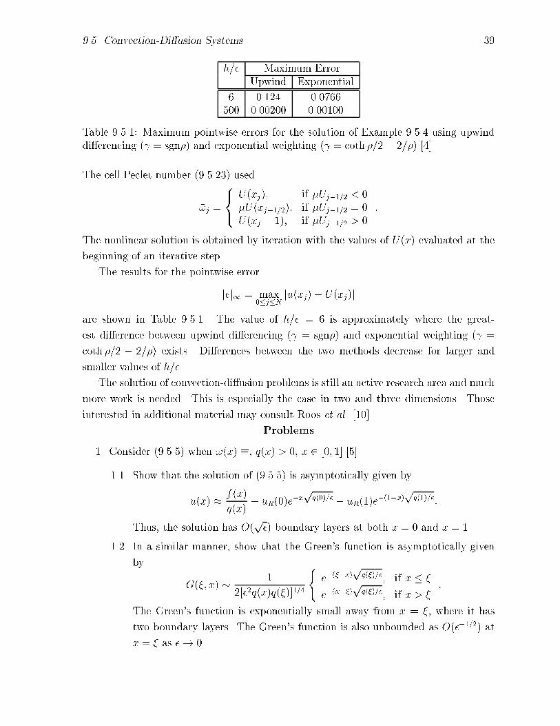
h�� Maximum ErrorUpwind Exponential
� ��� � ��������� ���� �� �������
Table ������ Maximum pointwise errors for the solution of Example ����� using upwinddi�erencing �� � sgn� and exponential weighting �� � coth �� � �� ����
The cell Peclet number ����� � used
��j �
���
U�xj� if �Uj���� � ��U�xj����� if �Uj���� � �U�xj � �� if �Uj���� � �
�
The nonlinear solution is obtained by iteration with the values of U�x evaluated at the
beginning of an iterative step�
The results for the pointwise error
jej� � max��j�N
ju�xj� U�xjj
are shown in Table ������ The value of h�� � � is approximately where the great�
est di�erence between upwind di�erencing �� � sgn� and exponential weighting �� �
coth �� � �� exists� Di�erences between the two methods decrease for larger and
smaller values of h���
The solution of convection�di�usion problems is still an active research area and much
more work is needed� This is especially the case in two and three dimensions� Those
interested in additional material may consult Roos et al� �����
Problems
�� Consider ������ when ��x � q�x � � x � ��� �� ����
���� Show that the solution of ������ is asymptotically given by
u�x � f�x
q�x� uR��e
�xp
q����� � uR��e����x�
pq������
Thus the solution has O�p� boundary layers at both x � � and x � ��
�� � In a similar manner show that the Green�s function is asymptotically given
by
G��� x � �
���q�xq�����
�e����x�
pq������ if x � �
e��x���p
q������ if x � ��
The Green�s function is exponentially small away from x � � where it has
two boundary layers� The Green�s function is also unbounded as O������ at
x � � as �� ��

�� Parabolic Problems

Bibliography
��� S� Adjerid M� Ai�a and J�E� Flaherty� Computational methods for singularly per�
turbed systems� In J�D� Cronin and Jr� R�E� O�Malley editors Analyzing Multiscale
Phenomena Using Singular Perturbation Methods volume �� of Proceedings of Sym�
posia in Applied Mathematics pages ��$�� Providence ����� AMS�
� � U�M� Ascher and L�R� Petzold� Computer Methods for Ordinary Di�erential Equa�
tions and Di�erential�Algebraic Equations� SIAM Philadelphia �����
��� K�E� Brenan S�L Campbell and L�R� Petzold� Numerical Solution of Initial�Value
Problems in Di�erential�Algebraic Equations� North Holland New York �����
��� J�E� Flaherty� A rational function approximation for the integration point in ex�
ponentially weighted �nite element methods� International Journal of Numerical
Methods in Engineering ����� $��� ��� �
��� J�E� Flaherty and W� Mathon� Collocation with polynomial and tension splines for
singularly�perturbed boundary value problems� SIAM Journal on Scie�nti c and
Statistical Computation �� ��$ �� �����
��� C�W� Gear� Numerical Initial Value Problems in Ordinary Di�erential Equations�
Prentice Hall Englewood Cli�s �����
��� E� Hairer S�P� Norsett and G� Wanner� Solving Ordinary Di�erential Equations I�
Nonsti� Problems� Springer�Verlag Berlin second edition �����
��� E� Hairer and G� Wanner� Solving Ordinary Di�erential Equations II� Sti� and
Di�erential Algebraic Problems� Springer�Verlag Berlin �����
��� C� Johnson� Numerical Solution of Partial Di�erential Equations by the Finite Ele�
ment method� Cambridge Cambridge �����
���� H��G� Roos M� Stynes and L� Tobiska� Numerical Methods for Singularly Perturbed
Di�erential Equations� Springer�Verlag Berlin �����
��
![Untitled 10052017 125101 [medical-office-qatar.de]medical-office-qatar.de/downloads/news5.pdf · JL..i - - 18 — 65 . 12 - a.4Lž 24 L. a-NS . IgnJI tn ÖISIA! O JbIJnJIg LÞ.»n1J](https://img.pdfslide.us/doc/110x75/60ba22a4c0c2b4050e20caf8/untitled-10052017-125101-medical-office-qatardemedical-office-qatardedownloadsnews5pdf.jpg)


![1 In - public.lanl.gov · as recti ed in [10], [4], and [3] with sc hemes that in v olv ed explicit treatmen t of the appropriate b oundary conditions at the in terface. As a consequence,](https://img.pdfslide.us/doc/110x75/5d02b2f988c99388628cc493/1-in-as-recti-ed-in-10-4-and-3-with-sc-hemes-that-in-v-olv-ed-explicit.jpg)