Chapterflaherje/pdf/fea1.pdf · Chapter and it has no w b ecome one of the most imp ortan t n ... tb y writing v L All functions of class ... 1

Chapter �

Introduction

�� Historical Perspective

The �nite element method is a computational technique for obtaining approximate solu�

tions to the partial di�erential equations that arise in scienti�c and engineering applica�

tions� Rather than approximating the partial di�erential equation directly as with� e�g��

�nite di�erence methods� the �nite element method utilizes a variational problem that

involves an integral of the di�erential equation over the problem domain� This domain

is divided into a number of subdomains called �nite elements and the solution of the

partial di�erential equation is approximated by a simpler polynomial function on each

element� These polynomials have to be pieced together so that the approximate solution

has an appropriate degree of smoothness over the entire domain� Once this has been

done� the variational integral is evaluated as a sum of contributions from each �nite el�

ement� The result is an algebraic system for the approximate solution having a �nite

size rather than the original in�nite�dimensional partial di�erential equation� Thus� like

�nite di�erence methods� the �nite element process has discretized the partial di�eren�

tial equation but� unlike �nite di�erence methods� the approximate solution is known

throughout the domain as a pieceise polynomial function and not just at a set of points�

Logan �� attributes the discovery of the �nite element method to Hrennikof �� and

McHenry �� who decomposed a two�dimensional problem domain into an assembly of

one�dimensional bars and beams� In a paper that was not recognized for several years�

Courant �� used a variational formulation to describe a partial di�erential equation with

a piecewise linear polynomial approximation of the solution relative to a decomposition of

the problem domain into triangular elements to solve equilibrium and vibration problems�

This is essentially the modern �nite element method and represents the �rst application

where the elements were pieces of a continuum rather than structural members�

Turner et al� �� wrote a seminal paper on the subject that is widely regarded

�

� Introduction

as the beginning of the �nite element era� They showed how to solve one� and two�

dimensional problems using actual structural elements and triangular� and rectangular�

element decompositions of a continuum� Their timing was better than Courant s ��

since success of the �nite element method is dependent on digital computation which

was emerging in the late ��s� The concept was extended to more complex problems

such as plate and shell deformation �cf� the historical discussion in Logan �� Chapter

�� and it has now become one of the most important numerical techniques for solving

partial di�erential equations� It has a number of advantages relative to other methods�

including

� the treatment of problems on complex irregular regions�

� the use of nonuniform meshes to re�ect solution gradations�

� the treatment of boundary conditions involving �uxes� and

� the construction of high�order approximations�

Originally used for steady �elliptic� problems� the �nite element method is now used

to solve transient parabolic and hyperbolic problems� Estimates of discretization errors

may be obtained for reasonable costs� These are being used to verify the accuracy of the

computation� and also to control an adaptive process whereby meshes are automatically

re�ned and coarsened and�or the degrees of polynomial approximations are varied so as

to compute solutions to desired accuracies in an optimal fashion ��

�� Weighted Residual Methods

Our goal� in this introductory chapter� is to introduce the basic principles and tools of

the �nite element method using a linear two�point boundary value problem of the form

L�u� �� d

dx�p�x�

du

dx� � q�x�u � f�x�� x � �� a�

u�� u�� b�

The �nite element method is primarily used to address partial di�erential equations and is

hardly used for two�point boundary value problems� By focusing on this problem� we hope

to introduce the fundamental concepts without the geometric complexities encountered

in two and three dimensions�

Problems like �� arise in many situations including the longitudinal deformation

of an elastic rod� steady heat conduction� and the transverse de�ection of a supported

�� Weighted Residual Methods �

cable� In the latter case� for example� u�x� represents the lateral de�ection at position

x of a cable having �scaled� unit length that is subjected to a tensile force p� loaded by

a transverse force per unit length f�x�� and supported by a series of springs with elastic

modulus q �Figure �� The situation resembles the cable of a suspension bridge� The

tensile force p is independent of x for the assumed small deformations of this model� but

the applied loading and spring moduli could vary with position�

��

��

q(x) u(x)

xpp

f(x)

Figure �� De�ection u of a cable under tension p� loaded by a force f per unit length�and supported by springs having elastic modulus q�

Mathematically� we will assume that p�x� is positive and continuously di�erentiable

for x � �� q�x� is non�negative and continuous on �� and f�x� is continuous on

��

Even problems of this simplicity cannot generally be solved in terms of known func�

tions� thus� the �rst topic on our agenda will be the development of a means of calculating

approximate solutions of �� With �nite di�erence techniques� derivatives in ��a�

are approximated by �nite di�erences with respect to a mesh introduced on ��

With the �nite element method� the method of weighted residuals �MWR� is used to

construct an integral formulation of �� called a variational problem� To this end� let

us multiply ��a� by a test or weight function v and integrate over �� to obtain

�v�L�u�� f� � �� a�

We have introduced the L� inner product

�v� u� ��

Z�

�

vudx ��b�

to represent the integral of a product of two functions�

The solution of �� is also a solution of ��a� for all functions v for which the

inner product exists� We ll express this requirement by writing v � L�� All functions

of class L�� are �square integrable� on �� thus� �v� v� exists� With this viewpoint

and notation� we write ��a� more precisely as

�v�L�u�� f� � �� v � L�� c�

� Introduction

Equation ��c� is referred to as a variational form of problem �� The reason for

this terminology will become clearer as we develop the topic�

Using the method of weighted residuals� we construct approximate solutions by re�

placing u and v by simpler functions U and V and solving ��c� relative to these

choices� Speci�cally� we ll consider approximations of the form

u�x� � U�x� �NXj��

cj�j�x�� a�

v�x� � V �x� �NXj��

dj�j�x�� b�

The functions �j�x� and �j�x�� j � �� N � are preselected and our goal is to

determine the coe�cients cj� j � �� N � so that U is a good approximation of u�

For example� we might select

�j�x� � �j�x� � sin j�x� j � �� N�

to obtain approximations in the form of discrete Fourier series� In this case� every function

satis�es the boundary conditions ��b�� which seems like a good idea�

The approximation U is called a trial function and� as noted� V is called a test func�

tion� Since the di�erential operator L�u� is second order� we might expect u � C��

�Actually� u can be slightly less smooth� but C� will su�ce for the present discussion��

Thus� it s natural to expect U to also be an element of C�� Mathematically� we re�

gard U as belonging to a �nite�dimensional function space that is a subspace of C��

We express this condition by writing U � SN�� C�� The restriction of these

functions to the interval � � x � � will� henceforth� be understood and we will no longer

write the �� With this interpretation� we ll call SN the trial space and regard the

preselected functions �j�x�� j � �� N � as forming a basis for SN �

Likewise� since v � L�� we ll regard V as belonging to another �nite�dimensional

function space �SN called the test space� Thus� V � �SN � L� and �j�x�� j � �� N �

provide a basis for �SN �

Now� replacing v and u in ��c� by their approximations V and U � we have

�V�L�U �� f� � �� V � �SN � ��a�

The residual

r�x� �� L�U �� f�x� ��b�


is apparent and clari�es the name �method of weighted residuals�� The vanishing of the

inner product ��a� implies that the residual is orthogonal in L� to all functions V in

the test space �SN �

Substituting �� into ��a� and interchanging the sum and integral yields

NXj��

dj��j�L�U �� f� � �� dj� j � �� N� ��

Having selected the basis �j� j � �� N � the requirement that ��a� be satis�ed for

all V � �SN implies that �� be satis�ed for all possible choices of dk� k � �� N �

This� in turn� implies that

��j�L�U �� f� � �� j � �� N� ��

Shortly� by example� we shall see that �� represents a linear algebraic system for the

unknown coe�cients ck� k � �� N �

One obvious choice is to select the test space �SN to be the same as the trial space

and use the same basis for each� thus� �k�x� � �k�x�� k � �� N � This choice leads

to Galerkin�s method

��j�L�u�� f� � �� j � �� N� ��

which� in a slightly di�erent form� will be our �work horse�� With �j � C�� j �

�� N � the test space clearly has more continuity than necessary� Integrals like

�� or �� exist for some pretty �wild� choices of V � Valid methods exist when V

is a Dirac delta function �although such functions are not elements of L�� and when V

is a piecewise constant function �cf� Problems � and � at the end of this section��

There are many reasons to prefer a more symmetric variational form of �� than

�� e�g�� problem �� is symmetric �self�adjoint� and the variational form should

re�ect this� Additionally� we might want to choose the same trial and test spaces� as with

Galerkin s method� but ask for less continuity on the trial space SN � This is typically

the case� As we shall see� it will be di�cult to construct continuously di�erentiable

approximations of �nite element type in two and three dimensions� We can construct

the symmetric variational form that we need by integrating the second derivative terms

in ��a� by parts� thus� using ��a�Z�

�

v��pu�� qu� f �dx �

Z�

�

�v�pu� � vqu� vf�dx� vpu�j��

where � �� d� ��dx� The treatment of the last �boundary� term will need greater

attention� For the moment� let v satisfy the same trivial boundary conditions ��b� as

Introduction

u� In this case� the boundary term vanishes and �� becomes

A�v� u�� v� f� � � ��a�

where

A�v� u� �

Z�

�

�v�pu� � vqu�dx� ��b�

The integration by parts has eliminated second derivative terms from the formulation�

Thus� solutions of �� might have less continuity than those satisfying either �� or

�� For this reason� they are called weak solutions in contrast to the strong solutions

of �� or �� Weak solutions may lack the continuity to be strong solutions� but

strong solutions are always weak solutions� In situations where weak and strong solutions

di�er� the weak solution is often the one of physical interest�

Since we ve added a derivative to v by the integration by parts� v must be restricted

to a space where functions have more continuity than those in L�� Having symmetry in

mind� we will select functions u and v that produce bounded values of

A�u� u� �

Z�

�

�p�u�� qu��dx�

Actually� since p and q are smooth functions� it su�ces for u and v to have bounded

values of Z�

�

��u�� u��dx� ��

Functions where �� exists are said to be elements of the Sobolev space H�� We ve

also required that u and v satisfy the boundary conditions ��b�� We identify those

functions in H� that also satisfy ��b� as being elements of H�� Thus� in summary�

the variational problem consists of determining u � H�� such that

A�v� u� � �v� f�� v � H�

� � ��

The bilinear form A�v� u� is called the strain energy� In mechanical systems it frequently

corresponds to the stored or internal energy in the system�

We obtain approximate solutions of �� in the manner described earlier for the

more general method of weighted residuals� Thus� we replace u and v by their approxi�

mations U and V according to �� Both U and V are regarded as belonging to the

same �nite�dimensional subspace SN� of H�� and �j� j � �� N � forms a basis for

SN� � Thus� U is determined as the solution of

A�V� U� � �V� f�� V � SN� � ��a�


The substitution of ��b� with �j replaced by �j in ��a� again reveals the more

explicit form

A��j� U� � ��j� f�� j � �� N� ��b�

Finally� to make ��b� totally explicit� we eliminate U using ��a� and interchange

a sum and integral to obtain

NXk��

ckA��j� �k� � ��j� f�� j � �� N� ��c�

Thus� the coe�cients ck� k � �� N � of the approximate solution ��a� are deter�

mined as the solution of the linear algebraic equation ��c�� Di�erent choices of the

basis �j� j � �� N � will make the integrals involved in the strain energy ��b�

and L� inner product ��b� easy or di�cult to evaluate� They also a�ect the accuracy

of the approximate solution� An example using a �nite element basis is presented in the

next section�

Problems

�� Consider the variational form �� and select

�j�x� � ��x� xj�� j � �� N�

where ��x� is the Dirac delta function satisfying

��x� � �� x ��

Z�

��

��x�dx � ��

and

� � x� � x� � � � � � xN � ��

Show that this choice of test function leads to the collocation method

L�U �� f�x�jx�xj � �� j � �� N�

Thus� the di�erential equation �� is satis�ed exactly at N distinct points on

��

�� The subdomain method uses piecewise continuous test functions having the basis

�j�x� ��

�� if x � �xj�� xj�� otherwise

�

where xj�� xj � xj�� Using �� show that the approximate solution

U�x� satis�es the di�erential equation ��a� on the average on each subinterval

�xj�� xj�� j � �� N �

Introduction

�� Consider the two�point boundary value problem

�u�� u � x� � � x � �� u�� u��

which has the exact solution

u�x� � x�sinh x

sinh ��

Solve this problem using Galerkin s method ��c� using the trial function

U�x� � c� sin�x�

Thus� N � �� x� � ��x� � sin�x in �� Calculate the error in strain

energy as A�u� u�� A�U� U�� where A�u� v� is given by ��b��

�� A Simple Finite Element Problem

Finite element methods are weighted residuals methods that use bases of piecewise poly�

nomials having small support� Thus� the functions ��x� and ��x� of �� are

nonzero only on a small portion of problem domain� Since continuity may be di�cult to

impose� bases will typically use the minimum continuity necessary to ensure the existence

of integrals and solution accuracy� The use of piecewise polynomial functions simplify

the evaluation of integrals involved in the L� inner product and strain energy ��b�

��b� and help automate the solution process� Choosing bases with small support leads

to a sparse� well�conditioned linear algebraic system ��c�� for the solution�

Let us illustrate the �nite element method by solving the two�point boundary value

problem �� with constant coe�cients� i�e��

�pu�� qu � f�x�� x � �� u�� u��

where p � � and q � �� As described in Section �� we construct a variational form of

�� using Galerkin s method �� For this constant�coe�cient problem� we seek

to determine u � H�� satisfying

A�v� u� � �v� f�� v � H�

� � ��a�

where

�v� u� �

Z�

�

vudx� ��b�

A�v� u� �

Z�

�

�v�pu� � vqu�dx� ��c�

�� A Simple Finite Element Problem �

With u and v belonging to H�� we are sure that the integrals ��b�c� exist and that

the trivial boundary conditions are satis�ed�

We will subsequently show that functions �of one variable� belonging to H� must

necessarily be continuous� Accepting this for the moment� let us establish the goal of

�nding the simplest continuous piecewise polynomial approximations of u and v� This

would be a piecewise linear polynomial with respect to a mesh

� � x� � x� � � � � � xN � � ��

introduced on �� Each subinterval �xj�� xj�� j � �� N � is called a �nite element�

The basis is created from the �hat function�

�j�x� �

��

x�xj��xj�xj��

� if xj�� x � xjxj��x

xj��xj� ifxj � x � xj��

�� otherwise

� ��a�

x x x x

1

x

jj-10 j+1

j(x)

Nx

φ

Figure �� One�dimensional �nite element mesh and piecewise linear hat function�j�x��

As shown in Figure �� j�x� is nonzero only on the two elements containing the

node xj� It rises and descends linearly on these two elements and has a maximal unit

value at x � xj� Indeed� it vanishes at all nodes but xj� i�e��

�j�xk� � �jk ��

�� if xk � xj�� otherwise

� ��b�

Using this basis with �� we consider approximations of the form

U�x� �N��Xj��

cj�j�x��

Let s examine this result more closely�

�� Introduction

x x x x x

x

jj-10 j+1 N

φj(x)φ

j-1(x)

c

c

jj-1

j+1

c

1

U(x)

Figure �� Piecewise linear �nite element solution U�x��

�� Since each �j�x� is a continuous piecewise linear function of x� their summation

U is also continuous and piecewise linear� Evaluating U at a node xk of the mesh

using ��b� yields

U�xk� �N��Xj��

cj�j�xk� � ck�

Thus� the coe�cients ck� k � �� N � �� are the values of U at the interior

nodes of the mesh �Figure ��

�� By selecting the lower and upper summation indices as � and N�� we have ensured

that �� satis�es the prescribed boundary conditions

U�� U��

As an alternative� we could have added basis elements ��x� and �N�x� to the

approximation and written the �nite element solution as

U�x� �NXj��

cj�j�x��

Since� using ��b�� U�x�� c� and U�xN � � cN � the boundary conditions are

satis�ed by requiring c� � cN � �� Thus� the representations �� or �� are

identical� however� �� would be useful with non�trivial boundary data�

�� The restriction of the �nite element solution �� or �� to the element

�xj�� xj� is the linear function

U�x� � cj��j��x� � cj�j�x�� x � �xj�� xj��

�� A Simple Finite Element Problem ��

since �j�� and �j are the only nonzero basis elements on �xj�� xj� �Figure ��

Using Galerkin s method in the form ��c�� we have to solve

N��Xk��

ckA��j� �k� � ��j� f�� j � �� N � ��

Equation �� can be evaluated in a straightforward manner by substituting replacing

�k and �j using �� and evaluating the strain energy and L� inner product according

to ��b�c�� This development is illustrated in several texts �e�g�� Section ��

We ll take a slightly more complex path to the solution in order to focus on the computer

implementation of the �nite element method� Thus� write ��a� as the summation of

contributions from each element

NXj��

�Aj�V� U�� V� f�j� � �� V � SN� � ��a�

where

Aj�V� U� � ASj �V� U� � AM

j �V� U�� b�

ASj �V� U� �

Z xj

xj��

pV �U �dx� ��c�

AMj �V� U� �

Z xj

xj��

qV Udx� ��d�

�V� f�j �

Z xj

xj��

V fdx� ��e�

It is customary to divide the strain energy into two parts with ASj arising from internal

energies and AMj arising from inertial e�ects or sources of energy�

Matrices are simple data structures to manipulate on a computer� so let us write the

restriction of U�x� to �xj�� xj� according to �� as

U�x� � �cj�� cj�

��j��x��j�x�

�� j��x�� j�x��

�cj��cj

�� x � �xj�� xj�� a�

We can� likewise� use ��b� to write the restriction of the test function V �x� to �xj�� xj�

in the same form

V �x� � �dj�� dj�

��j��x��j�x�

�� j��x�� j�x��

�dj��dj

�� x � �xj�� xj�� b�

�� Introduction

Our task is to substitute �� into ��c�e� and evaluate the integrals� Let us begin

by di�erentiating ��a� while using ��a� to obtain

U ��x� � �cj�� cj�

��hj��hj

�� hj� ��hj�

�cj��cj

�� x � �xj�� xj�� a�

where

hj � xj � xj�� j � �� N� ��b�

Thus� U ��x� is constant on �xj�� xj� and is given by the �rst divided di�erence

U ��x� �cj � cj��

hj� x � �xj�� xj��

Substituting �� and a similar expression for V ��x� into ��b� yields

ASj �V� U� �

Z xj

xj��

p�dj�� dj�

��hj��hj

��hj� ��hj�

�cj��cj

�dx

or

ASj �V� U� � �dj�� dj�

�Z xj

xj��

p

��h�j ��h�j

��h�j ��h�j

�dx

��cj��cj

��

The integrand is constant and can be evaluated to yield

ASj �V� U� � �dj�� dj�Kj

�cj��cj

�� Kj �

p

hj

��

��

��

The � � matrix Kj is called the element sti�ness matrix� It depends on j through hj�

but would also have such dependence if p varied with x� The key observation is that

Kj can be evaluated without knowing cj�� cj� dj�� or dj and this greatly simpli�es the

automation of the �nite element method�

The evaluation of AMj proceeds similarly by substituting �� into ��d� to

obtain

AMj �V� U� �

Z xj

xj��

q�dj�� dj�

��j��j

��j�� j�

�cj��cj

�dx�

With q a constant� the integrand is a quadratic polynomial in x that may be integrated

exactly �cf� Problem � at the end of this section� to yield

AMj �V� U� � �dj�� dj�Mj

cj��cj

� Mj �

qhj

��

��

whereMj is called the element mass matrix because� as noted� it often arises from inertial

loading�


The �nal integral ��e� cannot be evaluated exactly for arbitrary functions f�x��

Without examining this matter carefully� let us approximate it by its linear interpolant

f�x� � fj��j��x� � fj�j�x�� x � �xj�� xj��

where fj �� f�xj�� Substituting �� and ��b� into ��e� and evaluating the

integral yields

�V� f�j �

Z xj

xj��

�dj�� dj�

��j��j

��j�� j�

�fj��fj

�dx � �dj�� dj�lj ��a�

where

lj �hj

��fj�� fjfj�� fj

�� b�

The vector lj is called the element load vector and is due to the applied loading f�x��

The next step in the process is the substitution of �� and �� into

��a� and the summation over the elements� Since this our �rst example� we ll simplify

matters by making the mesh uniform with hj � h � ��N � j � �� N � and summing

ASj � A

Mj � and �V� f�j separately� Thus� summing ��

NXj��

ASj �

NXj��

�dj�� dj�p

h

��

��

� �cj��cj

��

The �rst and last contributions have to be modi�ed because of the boundary conditions

which� as noted� prescribe c� � cN � d� � dN � �� Thus�

NXj��

ASj � �d��

p

h��c�� d�� d��

p

h

��

��

� �c�c�

��

��dN�� dN��p

h

��

��

� �cN��cN��

�� dN��

p

h��cN��

Although this form of the summation can be readily evaluated� it obscures the need for the

matrices and complicates implementation issues� Thus� at the risk of further complexity�

we ll expand each matrix and vector to dimension N � � and write the summation as

NXk��

ASj � �d�� d�� dN��

p

h

��

��

c�c��

cN��

��

�� Introduction

��d�� d�� dN��p

h

��

� ��

��

c�c��

cN��

��

� � �d�� d�� dN��p

h

��

��

��

c�c��

cN��

��

��d�� d�� dN��p

h

��

�

��

c�c��

cN��

��

Zero elements of the matrices have not been shown for clarity� With all matrices and

vectors having the same dimension� the summation is

NXj��

ASj � d

TKc� ��a�

where

K �p

h

��

� ��

��

��

�� b�

c � �c�� c�� cN��T � ��c�

d � �d�� d�� dN��T � ��d�

The matrix K is called the global sti�ness matrix� It is symmetric� positive de�nite� and

tridiagonal� In the form that we have developed the results� the summation over elements

is regarded as an assembly process where the element sti�ness matrices are added into

their proper places in the global sti�ness matrix� It is not necessary to actually extend the

dimensions of the element matrices to those of the global sti�ness matrix� As indicated

in Figure �� the elemental indices determine the proper location to add a local matrix

into the global matrix� Thus� the � � element sti�ness matrix Kj is added to rows


AS� � d�

p

h��z� c� AS

� � �d�� d��p

h

��

��

�� z �

�c�c�

�

AS� � �d�� d��

p

h

��

��

�� z �

�c�c�

�

K �p

h

��

� ��

��

��

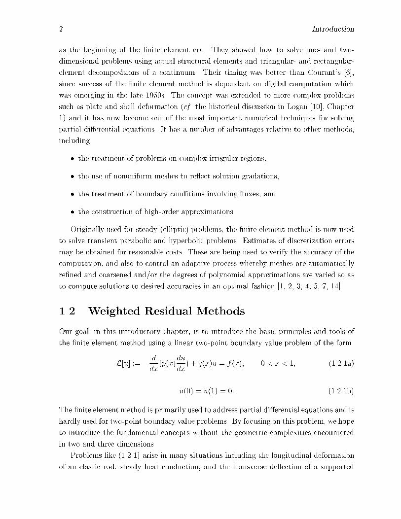
Figure �� Assembly of the �rst three element sti�ness matrices into the global sti�nessmatrix�

j � � and j and columns j � � and j� Some modi�cations are needed for the �rst and

last elements to account for the boundary conditions�

The summations of AMj and �V� f�j proceed in the same manner and� using ��

and �� we obtain

NXj��

AMj � d

TMc� ��a�

NXj��

�V� f�j � dTl ��b�

where

M �qh

��

� ��

� � ��

� � �

� � ��

�� c�

l �h

��

f� � �f� � f�f� � �f� � f�

��fN�� fN�� fN

�� d�

� Introduction

The matrix M and the vector l are called the global mass matrix and global load vector�

respectively�

Substituting ��a� and ��a�b� into ��a�b� gives

dT ��K�M�c� l� � ��

As noted in Section �� the requirement that ��a� hold for all V � SN� is equivalent

to satisfying �� for all choices of d� This is only possible when

�K�M�c � l� ��

Thus� the nodal values ck� k � �� N � �� of the �nite element solution are deter�

mined by solving a linear algebraic system� With c known� the piecewise linear �nite

element U can be evaluated for any x using ��a�� The matrix K �M is symmetric�

positive de�nite� and tridiagonal� Such systems may be solved by the tridiagonal algo�

rithm �cf� Problem � at the end of this section� in O�N� operations� where an operation

is a scalar multiply followed by an addition�

The discrete system �� is similar to the one that would be obtained from a

centered �nite di�erence approximation of �� which is ��

�K�D��c � �l� ��a�

where

D � qh

��

��

� � �

�

�� l � h

��

f�f��

fN��

�� c �

��

�c��c��

�cN��

�� b�

Thus� the qu and f terms in �� are approximated by diagonal matrices with the

�nite di�erence method� In the �nite element method� they are �smoothed� by coupling

diagonal terms with their nearest neighbors using Simpson s rule weights� The diagonal

matrix D is sometimes called a �lumped� approximation of the consistent mass matrix

M� Both �nite di�erence and �nite element solutions behave similarly for the present

problem and have the same order of accuracy at the nodes of a uniform mesh�

Example �� Consider the �nite element solution of

�u�� u � x� � � x � �� u�� u��

which has the exact solution

u�x� � x�sinh x

sinh ��


Relative to the more general problem �� this example has p � q � � and f�x� � x�

We solve it using the piecewise�linear �nite element method developed in this section on

uniform meshes with spacing h � ��N for N � �� Before presenting results�

it is worthwhile mentioning that the load vector �� is exact for this example� Even

though we replaced f�x� by its piecewise linear interpolant according to �� this

introduced no error since f�x� is a linear function of x�

Letting

e�x� � u�x�� U�x� ��

denote the discretization error in Table �� we display the maximum error of the �nite

element solution and of its �rst derivative at the nodes of a mesh� i�e��

jej� �� max��j�N

je�xj�j� je�j� �� max��j�N

je��x�j �j� ��

We have seen that U ��x� is a piecewise constant function with jumps at nodes� Data in

Table �� were obtained by using derivatives from the left� i�e�� x�j � lim�� xj�� With

this interpretation� the results of second and fourth columns of Table �� indicate that

jej��h� and je�j��h are �essentially� constants� hence� we may conclude that jej� � O�h��

and je�j� � O�h��

N jej� jej��h� je�j� je�j��h

� ��

Table �� Maximum nodal errors of the piecewise�linear �nite element solution and itsderivative for Example �� Numbers in parenthesis indicate a power of ��

The �nite element and exact solutions of this problem are displayed in Figure �� for

a uniform mesh with eight elements� It appears that the pointwise discretization errors

are much smaller at nodes than they are globally� We ll see that this phenomena� called

superconvergence� applies more generally than this single example would imply�

Since �nite element solutions are de�ned as continuous functions �of x�� we can also

appraise their behavior in some global norms in addition to the discrete error norms used

in Table �� Many norms could provide useful information� One that we will use quite

� Introduction

0 0.1 0.2 0.3 0.4 0.5 0.6 0.7 0.8 0.9 10

0.01

0.02

0.03

0.04

0.05

0.06

Figure �� Exact and piecewise�linear �nite element solutions of Example �� on an�element mesh�

often is the square root of the strain energy of the error� thus� using ��c�

kekA ��pA�e� e� �

�Z�

�

�p�e�� qe��dx

��

� ��a�

This expression may easily be evaluated as a summation over the elements in the spirit

of ��a�� With p � q � � for this example�

kek�A �

Z�

�

��e�� e��dx�

The integral is the square of the norm used on the Sobolev space H�� thus�

kek� ��

�Z�

�

��e�� e��dx

��

� ��b�

Other global error measures will be important to our analyses� however� the only one


that we will introduce at the moment is the L� norm

kek� ��

�Z�

�

e��x�dx

�� c�

Results for the L� and strain energy errors� presented in Table �� for this example�

indicate that kek� � O�h�� and kekA � O�h�� The error in the H� norm would be

identical to that in strain energy� Later� we will prove that these a priori error estimates

are correct for this and similar problems� Errors in strain energy converge slower than

those in L� because solution derivatives are involved and their nodal convergence is O�h�

�Table ��

N kek� kek��h� kekA kekA�h

� ��

Table �� Errors in L� and strain energy for the piecewise�linear �nite element solutionof Example �� Numbers in parenthesis indicate a power of ��

Problems

�� The integral involved in obtaining the mass matrix according to �� may� of

course� be done symbolically� It may also be evaluated numerically by Simpson s

rule which is exact in this case since the integrand is a quadratic polynomial� Recall�

that Simpson s rule isZ h

�

F�x�dx �h

�F�� F�h�� F�h��

The mass matrix is

Mj �

Z xj

xj��

��j��j

��j�� j�dx�

Using �� determine Mj by Simpson s rule to verify the result �� The

use of Simpson s rule may be simpler than symbolic integration for this example

since the trial functions are zero or unity at the ends of an element and one half at

its center�

�� Consider the solution of the linear system

AX � F� ��a�

�� Introduction

where F and X are N �dimensional vectors and A is an N N tridiagonal matrix

having the form

A �

�� a� c�b� a� c�

� � � � � � � � �

bN�� aN�� cN��bN aN

�� b�

Assume that pivoting is not necessary and factor A as

A � LU� ��a�

where L and U are lower and upper bidiagonal matrices having the form

L �

��

�l� �

l� ��

lN �

�� b�

U �

�� u� v�

u� v��

uN�� vN��uN

�� c�

Once the coe�cients lj� j � �� N � uj� j � �� N � and vj� j � �� N�

�� have been determined� the system ��a� may easily be solved by forward and

backward substitution� Thus� using ��a� in ��a� gives

LUX � F� ��a�

Let

UX � Y� ��b�

then�

LY � F� ��c�

�� Using �� and �� show

u� � a��

lj � bj�uj�� uj � aj � ljcj�� j � �� N�

vj � cj� j � �� N�


�� Show that Y and X are computed as

Y� � F��

Yj � Fj � ljYj�� j � �� N�

XN � yN�uN �

Xj � �Yj � vjXj��uj� j � N � �� N � ��

�� Develop a procedure to implement this scheme for solving tridiagonal systems�

The input to the procedure should be N and vectors containing the coe�cients

aj� bj� cj� fj� j � �� N � The procedure should output the solution X�

The coe�cients aj� bj� etc�� j � �� N � should be replaced by uj� vj� etc��

j � �� N � in order to save storage� If you want� the solution X can be

returned in F�

�� Estimate the number of arithmetic operations necessary to factor A and for

the forward and backward substitution process�

�� Consider the linear boundary value problem

�pu�� qu � f�x�� x � �� u�� u��

where p and q are positive constants and f�x� is a smooth function�

�� Show that the Galerkin form of this boundary�value problem consists of �nding

u � H�� satisfying

A�v� u�� v� f� �

Z�

�

�v�pu� � vqu�dx�

Z�

�

vfdx � �� v � H�

� �

For this problem� functions u�x� � H�� are required to be elements of H� and

satisfy the Dirichlet boundary condition u�� The Neumann boundary

condition at x � � need not be satis�ed by either u or v�

�� Introduce N equally spaced elements on � � x � � with nodes xj � jh�

j � �� N �h � ��N�� Approximate u by U having the form

U�x� �NXj��

ck�k�x��

where �j�x�� j � �� N � is the piecewise linear basis �� and use

Galerkin s method to obtain the global sti�ness and mass matrices and the

load vector for this problem� �Again� the approximation U�x� does not satisfy

the natural boundary condition u�� nor does it have to� We will discuss

this issue in Chapter ��

�� Introduction

�� Write a program to solve this problem using the �nite element method devel�

oped in Part ��b and the tridiagonal algorithm of Problem �� Execute your

program with p � �� q � �� and f�x� � x and f�x� � x�� In each case� use

N � �� and �� Let e�x� � u�x�� U�x� and� for each value of N � com�

pute jej�� je��xN �j� and kekA according to �� and ��a�� You may

�optionally� also compute kek� as de�ned by ��c�� In each case� estimate

the rate of convergence of the �nite element solution to the exact solution�

�� The Galerkin form of �� consists of determining u � H�� such that �� is

satis�ed� Similarly� the �nite element solution U � SN� � H�� satis�es ��

Letting e�x� � u�x�� U�x�� show

A�e� e� � A�u� u�� A�U� U�

where the strain energy A�v� u� is given by ��c�� We have� thus� shown that the

strain energy of the error is the error of the strain energy�

Bibliography

�� I� Babu�ska� J� Chandra� and J�E� Flaherty� editors� Adaptive Computational Methods

for Partial Di�erential Equations� Philadelphia� �� SIAM�

�� I� Babu�ska� O�C� Zienkiewicz� J� Gago� and E�R� de A� Oliveira� editors� Accuracy

Estimates and Adaptive Re�nements in Finite Element Computations� John Wiley

and Sons� Chichester� ��

�� M�W� Bern� J�E� Flaherty� and M� Luskin� editors� Grid Generation and Adaptive

Algorithms� volume �� of The IMA Volumes in Mathematics and its Applications�

New York� �� Springer�

�� G�F� Carey� Computational Grids Generation Adaptation and Solution Strategies�

Series in Computational and Physical Processes in Mechanics and Thermal science�

Taylor and Francis� New York� ��

�� K� Clark� J�E� Flaherty� and M�S� Shephard� editors� Applied Numerical Mathemat�

ics� volume �� Special Issue on Adaptive Methods for Partial Di�erential

Equations�

�� R� Courant� Variational methods for the solution of problems of equilibrium and

vibrations� Bulletin of the American Mathematics Society� ��

�� J�E� Flaherty� P�J� Paslow� M�S� Shephard� and J�D� Vasilakis� editors� Adaptive

methods for Partial Di�erential Equations� Philadelphia� �� SIAM�

�� A� Hrenniko�� Solutions of problems in elasticity by the frame work method� Journal

of Applied Mechanics� ��

�� C� Johnson� Numerical Solution of Partial Di�erential Equations by the Finite Ele�

ment method� Cambridge� Cambridge� ��

�� D�L� Logan� A First Course in the Finite Element Method using ALGOR� PWS�

Boston� ��

��

�� Introduction

�� D� McHenry� A lattice analogy for the solution of plane stress problems� Journal of

the Institute of Civil Engineers� ��

�� J�C� Strikwerda� Finite Di�erence Schemes and Partial Di�erential Equations�

Chapman and Hall� Paci�c Grove� ��

�� M�J� Turner� R�W� Clough� H�C� Martin� and L�J� Topp� Sti�ness and de�ection

analysis of complex structures� Journal of the Aeronautical Sciences� ��

��

�� R� Verf urth� A Review of Posteriori Error Estimation and Adaptive Mesh�

Re�nement Techniques� Teubner�Wiley� Stuttgart� ��

Documents

Chapterflaherje/pdf/fea1.pdf · Chapter and it has no w b ecome one of the most imp ortan t n ... tb y writing v L All functions of class ... 1