Embed Size (px)
Citation preview
OPERATIONS RESEARCHVol. 59, No. 2, March–April 2011, pp. 328–345issn 0030-364X �eissn 1526-5463 �11 �5902 �0328 doi 10.1287/opre.1100.0894
© 2011 INFORMS
Fixed-Point Approaches to Computing Bertrand-NashEquilibrium Prices Under Mixed-Logit Demand
W. Ross MorrowDepartments of Mechanical Engineering and Economics, Iowa State University, Ames, Iowa 50014, [email protected]
Steven J. SkerlosDepartment of Mechanical Engineering, University of Michigan, Ann Arhor, Michigan 48105, [email protected]
This article describes numerical methods that exploit fixed-point equations equivalent to the first-order condition forBertrand-Nash equilibrium prices in a class of differentiated product market models based on the mixed-logit model ofdemand. One fixed-point equation is already prevalent in the literature, and one is novel. Equilibrium prices are computedfor the calendar year 2005 new-vehicle market under two mixed-logit models using (i) a state-of-the-art variant of Newton’smethod applied to the first-order conditions as well as the two fixed-point equations and (ii) a fixed-point iteration generatedby our novel fixed-point equation. A comparison of the performance of these methods for a simple model with multipleequilibria is also provided. The analysis and trials illustrate the importance of using fixed-point forms of the first-orderconditions for efficient and reliable computations of equilibrium prices.
Subject classifications : Bertrand-Nash equilibrium prices; differentiated product markets; mixed logit; Newton’s method;GMRES-Newton hookstep; fixed-point iteration.
Area of review : Marketing Science.History : Received November 2008; revisions received August 2009, March 2010; accepted April 2010.
1. IntroductionBertrand competition has been a prominent paradigm forthe empirical study of differentiated product markets forat least 20 years. Firms engaged in Bertrand competitionmaximize profits by choosing prices for portfolios of dif-ferentiated products, and Bertrand-Nash equilibrium pricessimultaneously maximize profits for all firms. Models com-bining Bertrand competition with the mixed-logit discrete-choice model of consumer demand have been used tostudy the automotive industry, electronics, entertainment,and food products and services; see Dube et al. (2002).
Many applications of Bertrand competition rely on coun-terfactual experiments: exercises in which hypotheticalmarket conditions are simulated with an estimated model.Such experiments have been used to study corporate merg-ers (Nevo 2000a), novel products and services (Petrin2002, Goolsbee and Petrin 2004, Beresteanu and Li 2008),store locations (Thomadsen 2005), and regulatory policychanges (Goldberg 1995, 1998; Beresteanu and Li 2008).By definition, simulating market outcomes in counterfac-tual experiments requires computing equilibrium pricesafter changing the values of exogenous variables such asthe number of firms or the products offered. Numericalmethods for computing equilibrium prices have not yetreceived a thorough treatment in the literature, which cur-rently focuses on model specification and estimation; seeKnittel and Metaxoglou (2008), Dube et al. (2011), andSu and Judd (2008) for recent developments in estimation.
This article fills this gap with a detailed investigation offour approaches for computing Bertrand-Nash equilibriumprices in single-period, multifirm models with mixed-logitdemand.
Applying Newton’s method to some form of the first-order or “simultaneous stationarity” condition is currentlythe de facto approach for computing equilibrium prices;see, for example, Nevo (1997, 2000a), Petrin (2002), Smith(2004), Doraszelski and Draganska (2006), and Jacobsen(2006). Newton’s method applied directly to the first-ordercondition may converge when started at observed prices ifchanges in exogenous variables have a marginal impact onequilibrium prices. However, when the changes to exoge-nous variables imply significant changes in product prices,Newton’s method applied directly to the first-order condi-tions may fail to compute equilibrium prices. Furthermore,analyses that do not have observed prices to use as an initialguess will require methods with greater reliability.
This article demonstrates that solving fixed-point equa-tions equivalent to the first-order condition for equilibriumis more reliable and efficient than solving the first-ordercondition itself. One fixed-point equation equivalent to thefirst-order conditions is the BLP-markup equation popular-ized by Berry et al. (1995). A second fixed-point equa-tion, here termed the Æ-markup equation, is a novel way towrite the same condition on markups. Both markup equa-tions lead to more-robust numerical methods than foundwith a simple application of Newton’s method to thefirst-order condition. Using the fixed-point expressions in
328
Morrow and Skerlos: Fixed-Point Approaches to Computing Equilibrium PricesOperations Research 59(2), pp. 328–345, © 2011 INFORMS 329
this way can be considered “nonlinearly” or “analytically”preconditioning the first-order condition satisfied by equi-librium prices, a technique well known in applied mathe-matics (Brown and Saad 1990, Cai and Keyes 2002).
The existence of fixed-point equations for equilibriumsuggests applying fixed-point iteration (Judd 1998) insteadof Newton’s method to compute equilibrium prices. TheBLP-markup equation does not appear to be well suited tofixed-point iteration. Example 8 provides a case in whichiterating on the BLP-markup equation is not necessarilylocally convergent, whereas iterating on the Æ-markup equa-tion is superlinearly locally convergent. Iterating on theÆ-markup equation also eliminates the need to solve linearsystems, required to implement Newton’s method and toiterate on the BLP-markup equation. This property makesfixed-point steps based on the �-markup equation very inex-pensive relative to Newton steps, an essential property toobtaining fast computations from generally linearly conver-gent fixed-point iterations.
This fixed-point iteration is used to study the sensitivityof computed equilibrium prices to (i) the initial guess ofequilibrium prices and (ii) the finite sample set used forsimulation of a mixed-logit model (Train 2003). We findthat computed equilibrium prices vary little with the ini-tial guess, but are more sensitive to the sample set than iscurrently assumed. In one of our examples, computed equi-librium prices for roughly half of the products vary morethan $100 even with 100,000 samples; computed equilib-rium prices for 90% of products vary more than $1 evenwith 1,000,000 samples. Although the meaning of “preci-sion” depends on the application, these results suggest thatvariability due to simulation should receive more attentionthan it currently does.
Besides Newton’s method and fixed-point iteration, fewother practical approaches to the computation of equilib-rium prices exist. Variational formulations, widely appliedin economic and engineering problems (Ferris and Pang1997), contain many solutions that need not be equilib-ria of the original problem. Explicit least-square minimiza-tion or Gauss-Newton methods can also be implementedbut are computational disadvantages relative to applicationsof standard Newton-type methods for nonlinear systems.Some authors apply tattonement—iterating on a game’sbest-response correspondence—to compute equilibrium inprices or other strategic variables, including product mix(Choi et al. 1990), product characteristics (CBO 2003,Austin and Dinan 2005, Bento et al. 2005), and engineeringvariables (Michalek et al. 2004). Tattonement, however, hasthree issues: it requires the iterative computation of profit-optimal prices (a special case of the problem discussed inthis article), it should be inefficient relative to direct meth-ods whenever optimal strategies are coupled, and it lacksthe global convergence guarantees of contemporary Newtonsolvers. Morrow and Skerlos (2010) review these conclu-sions in more detail.
This article proceeds as follows: §2 describes Bertrandcompetition under mixed-logit models of demand. Itderives three representations of equilibrium prices: (i) thefirst-order or “simultaneous stationarity” condition, (ii) theBLP-markup equation, and (iii) the Æ-markup equation.Section 3 presents and motivates four numerical approachesfor computing equilibrium prices based on these represen-tations of the first-order condition. Section 4 compares thefour approaches in a numerical example with 993 vehiclessold during 2005 and provides a sensitivity study using anexpanded set of 5,298 vehicles. Section 5 addresses theperformance of these methods in a simple example wherethere are multiple equilibria. Many of the technical detailsare provided by Morrow and Skerlos (2010).
2. Fixed-Point Equations for EquilibriumPrices Under Mixed-Logit Models
This section derives the BLP- and Æ-markup equations for(local) equilibrium prices in differentiated product marketmodels with mixed-logit demand. Mixed-logit models arepopular in empirical applications and dense in the classof random utility models (RUM) (McFadden and Train2000). Our description of the mixed-logit model in §2.1 fol-lows Train (2003) and is more general than the descriptionnow standard in the empirical differentiated product mar-kets literature. This generality captures a variety of modelscurrently used in practice, as well as the finite-sample sim-ulators used both in estimation and computations of equi-librium prices (see Example 4). Sections 2.2 and 2.3 derivefirms’ profits and the first-order conditions for local equi-librium given this choice model; see also Nevo (2000b) orDube et al. (2002). Sections 2.4 and 2.5 derive the BLP-and Æ-markup equations from the first-order conditions.Tables 1 and 2 gives our nomenclature.
2.1. Consumers, Products, andChoice Probabilities
A collection of firms offer a total of J ∈ � products to apopulation of individuals (or households). Each product j ∈
J= 811 0 0 0 1 J 9 is defined by a price, pj ∈P= 601�5, anda vector of K ∈ � product “characteristics” xj ∈X⊂�K .Individuals are identified by a vector of characteristics Èfrom some set T. These individual characteristics caninclude both observed demographics and “random coeffi-cients” (Berry et al. 1995, Nevo 2000b, Train 2003) that
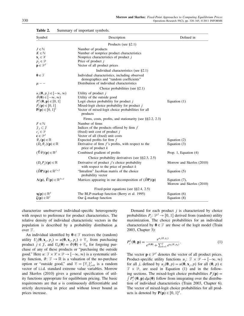
Table 1. Important sets.
Symbol Description
�= 81121 0 0 0 1 9 Natural numbers�= 4−�1�5 Real numbersP= 601�5 Nonnegative real numbersJ= 811 0 0 0 1 J 9 Set of product indicesX⊂�K Set of product characteristicsT⊂�L Set of individual characteristics
Morrow and Skerlos: Fixed-Point Approaches to Computing Equilibrium Prices330 Operations Research 59(2), pp. 328–345, © 2011 INFORMS
Table 2. Summary of important symbols.
Symbol Description Defined in
Products (see §2.1)J ∈� Number of productsK ∈� Number of nonprice product characteristicsxj ∈X Nonprice characteristics of product jpj ∈P Price of product jp ∈PJ Vector of all product prices
Individual characteristics (see §2.1)È ∈T Individual characteristics, including observed
demographics and “random coefficients”�− − Distribution of individual characteristics
Choice probabilities (see §2.1)uj4È1 pj5 ∈ 6−�1�5 Utility of product j�4È5 ∈ 6−�1�5 Utility of the outside goodPLj 4È1p5 ∈ 60117 Logit choice probability for product j Equation (1)
Pj4p5 ∈ 60117 Mixed-logit choice probability for product jP4p5 ∈ 60117J Vector of mixed-logit choice probabilities for all
products
Firms, costs, profits, and stationarity (see §§2.2, 2.3)F ∈� Number of firmsJf ⊂J Indices of the products offered by firm fcj ∈P (fixed) unit cost of product jc ∈PJ Vector of all (fixed) unit costsº�f 4p5 ∈� Expected profits for firm f Equation (2)4Dk º�f 54p5 ∈� Derivative of firm f ’s profits, with respect to the Equation (3)
price of product k4 ¶ï º�54p5 ∈�J Combined gradient of profits Prop. 1, Equation (4)
Choice probability derivatives (see §§2.3, 2.5)4DkPj54p5 ∈� Derivative of product j’s choice probability Morrow and Skerlos (2010)
with respect to the price of product k4 ¶DP54p5 ∈�J×J “Intrafirm” Jacobian matrix of the choice Equation (5)
probability vectorå4p5, ¶â4p5 ∈�J×J Matrices appearing in our decomposition of 4 ¶DP54p5 Equation (7),
Morrow and Skerlos (2010)
Fixed-point equations (see §§2.4, 2.5)Ç4p5 ∈�J The BLP-markup function (Berry et al. 1995) Equation (6)Æ4p5 ∈�J Our Æ-markup function Equation (8)
characterize unobserved individual-specific heterogeneitywith respect to preference for product characteristics. Therelative density of individual characteristic vectors in thepopulation is described by a probability distribution �over T.
An individual identified by È ∈T receives the (random)utility Uj4È1xj1 pj5 = u4È1xj1 pj5 + Ej from purchasingproduct j ∈ J, and U04È5 = �4È5 + E0 for forgoing pur-chase of any of these products or “purchasing the outsidegood.” Here u2 T×X×P→ 6−�1�5 is a systematic util-ity function, �2 T → � is a valuation of the no-purchaseoption or “outside good,” and E = 8Ej9
Jj=0 is a random
vector of i.i.d. standard extreme value variables. Morrowand Skerlos (2010) gives a general specification of util-ity functions appropriate for equilibrium pricing. The basicrequirements are that u is continuously differentiable andstrictly decreasing in price and without lower bound asprices increase.
Demand for each product j is characterized by choiceprobabilities Pj 2 P
J → 60117 derived from (random) utilitymaximization. The choice probabilities for an individualcharacterized by È ∈T are those of the logit model (Train2003, Chapter 3):
PLj 4È1p5=
euj 4�1pj 5
e�4È5 +∑J
k=1 euk4�1pk5
0 (1)
The vector p ∈PJ denotes the vector of all product prices.Product-specific utility functions uj 2 T × P → 6−�1�5for all j , defined by uj4È1 p5 = u4È1xj1 p5 for all 4È1 p5 ∈
T × P, are used in Equation (1) and in the follow-ing sections. The mixed-logit choice probabilities Pj4p5 =∫
PLj 4È1p5d�4È5 follow from integrating over the distribu-
tion of individual characteristics (Train 2003, Chapter 6).The vector of mixed-logit choice probabilities for all prod-ucts is denoted by P4p5 ∈ 60117J .
Morrow and Skerlos: Fixed-Point Approaches to Computing Equilibrium PricesOperations Research 59(2), pp. 328–345, © 2011 INFORMS 331
The examples below review several instances of thischoice model. Examples 1 and 2 are also used in §4 below.Example 3 illustrates the type general specifications used inestimation. Example 4 describes one kind of “simulation”of a mixed-logit model (Train 2003).
Example 1 (Boyd and Mellman 1980). Take T = P× �K , denoting È = 4�1Â5 for � ∈ P and  ∈ �K . Setu4�1Â1x1 p5 = −�p + Â>x and �4�1Â5 = −� for all4�1Â5 ∈ P×�K . � is defined by specifying that � and Âare independently lognormally distributed (with appropri-ately chosen signs, means, and variances). �
Example 2 (Berry et al. 1995). Take T=P×�K ×�,denoting È= 4�1Â1�05 for � ∈P,  ∈�K , and �0 ∈�. Set
u4�1Â1x1 p5=
{
� log4�−p5+Â>x if p <�1
−� otherwise1and
�4�1�05= � log�+�01
for some fixed coefficient �> 0. � represents income andis given a lognormal distribution, whereas the random coef-ficients Â1�0 are independently normally distributed withsome mean and variance. Note that income 4�5 serves asan upper bound on the price an individual can pay for anyproduct. �
Example 3 (Nevo 2000b). Take T = P × �D × �K+2,denoting È = 4�1d1Í5 for � ∈ P, d ∈ �D, and Í ∈ �K+2.Again, � represents income; d ∈ �D represents a vectorof D observed demographic variables (which may includeincome); Í ∈ �K+2 represents a vector of K + 2 randomcoefficients: one for each product characteristic, one forprice, and one for the outside good. Set
u4�1d1Í1x1 p5= 4�+Ï>
p d+Ñ>
p Í54�−p5
+ 4Â+çd+èÍ5>x
�4�1d1Í5= 4�+Ï>
p d+Ñ>
p Í5�+Ï>
0 d+Ñ>
0 Í1
where � ∈ �, Â ∈ �K , Ïp1Ï0 ∈ �D, ç ∈ �K×D, Ñp1Ñ0 ∈
�K+2, and è ∈ �K×4K+25 are coefficients. The distributionof d is estimated from available data (e.g., census data)and Í is assumed to be standard independent multivariatenormal. When �+Ï>
p d+Ñ>p Í, the coefficient on price, is
positive, an individual prefers higher prices.Petrin (2002) and Berry et al. (2004) adopt similar
specifications that eliminate this counterintuitive property.Petrin (2002) takes the price component of utility to be�4�5 log4�−p5, where �2 P→P is a step function. Berryet al. (2004) take the price component of utility to be �p,but define �= −e−4�+�>
p d+�>p �5. �
Example 4 (Simulation). Take any of the examplesabove, and draw S ∈ � vectors Ès ∈ T according to thedistribution �. Let T′ = 8Ès9
Ss=1, and define a probabil-
ity measure �′ over T′ by �′4Ès5 = 1/S for all s. Then
4u1�1T′1�′5 defines a simulator of the “full” mixed-logit model with 4u1�1T1�5; see Train (2003). Theseapproximations, discussed further in §3.5, are essential inestimation of mixed-logit models and in computations ofequilibrium prices. �
2.2. Firms, Costs, and Profits
Differentiated product market models are built from com-bining a model of choice, e.g., a mixed-logit model, witha model of firm behavior. There are F ∈ � firms, each ofwhich offers some subset of the J products offered to indi-viduals; Jf ⊂ J = 811 0 0 0 1 J 9 indexes the products offeredby firm f . In Bertrand competition, each firm f chooses theprices of the products they offer prior to some purchasingperiod in which consumers opt to purchase one, or none,of the products offered by all firms. All prices remain fixedduring this purchasing period, and firms satisfy all demand(Baye and Kovenock 2008).
Firms choose the prices of the products they offer tomaximize their expected profits
max º�f 4p5=∑
j∈Jf
Pj4p54pj − cj5
with respect to pj for all j ∈Jf (2)
where p ∈PJ denotes the vector of prices for all productsand cj denotes the constant unit cost of product j . The“stationarity” condition
4Dk º�f 54p5=∑
j∈Jf
4DkPj54p54pj − cj5+Pk4p5= 0
for all k ∈Jf (3)
is necessary for the prices of firm f ’s products to locallymaximize firm f ’s profits, for fixed competitor prices. Thiscondition requires that the mixed-logit choice probabilitiesare continuously differentiable in prices.
2.3. Local Equilibrium and the SimultaneousStationarity Conditions
Combining the stationarity condition for each firm weobtain the simultaneous stationarity condition, a first-order(necessary) condition for local equilibrium prices.
Proposition 1 (Simultaneous Stationarity Condi-tion). Suppose P is continuously differentiable. Let4 ¶ï º�54p5 ∈ �J denote the “combined gradient” with com-ponents 44 ¶ï º�54p55j = 4Dj º�f 4j554p5 where f 4j5 denotes theindex of the firm offering product j . If p is a local equilib-rium, then
4 ¶ï º�54p5= 4 ¶DP54p5>4p− c5+P4p5= 01 (4)
where 4 ¶DP54p5 ∈ �J×J is the “intrafirm” Jacobian matrixof price derivatives of the choice probabilities defined by
44 ¶DP54p55j1k
=
4DkPj54p5 if products j and k are offeredby the same firm1
0 otherwise0(5)
Morrow and Skerlos: Fixed-Point Approaches to Computing Equilibrium Prices332 Operations Research 59(2), pp. 328–345, © 2011 INFORMS
Prices p satisfying Equation (4) are called “simultaneouslystationary.”
The matrix −4 ¶DP54p5 has previously been denoted by“4” (Berry et al. 1995, Petrin 2002, Beresteanu and Li2008), “ì” (Nevo 2000a), and “ê” (Dube et al. 2002).We prefer the “D” notation to emphasize the relationshipof 4 ¶DP54p5 to the Jacobian matrix of the choice proba-bilities P, while using the superscript “∼” to denote theintrafirm sparsity structure.
A set of simultaneously stationary prices are a local equi-librium only if every firm’s profits are locally maximized atthose prices; this can be verified by confirming that everyfirm’s profits are locally concave. Note that there is no con-venient condition to verify that every firm’s profits are glob-ally maximized at a particular local equilibrium. That is,there is no convenient condition to ensure that certain pricesare a proper equilibrium.
2.4. The Markup Equation
A prominent form of the first-order conditions Equation (4)is the BLP-markup equation:
p= c+Ç4p5 where Ç4p5= −4 ¶DP54p5−>P4p50 (6)
Note that Ç is defined for any continuously differentiablechoice probabilities with nonsingular 4 ¶DP54p5>, such ascertain mixed-logit models (Morrow and Skerlos 2010).
Traditionally, the BLP-markup equation (6) has beenused to estimate costs assuming that observed prices are inequilibrium via the formula c = p−Ç4p5; see, e.g., Berryet al. (1995) or Nevo (2000a). These cost estimates formthe basis of counterfactual experiments with an estimateddemand model. Beresteanu and Li (2008) have recentlysuggested that the BLP-markup equation is also useful forcomputing equilibrium prices, a suggestion we explore fur-ther in §3.3 below. Note that the BLP-markup equationmust be interpreted as a nonlinear fixed-point equationwhen applied to compute equilibrium prices.
2.5. Another Fixed-Point Equation
In this section we derive our Æ-markup equation for equilib-rium using a particular decomposition of the choice prob-ability derivatives. Thus, this markup equation is specificto mixed-logit models, unlike the BLP-markup equation.First, Example 5 demonstrates this decomposition in a sim-ple case.
Example 5. Note that for simple logit,
4DkPLj 54p5= �j1 k4Dkuk54pk5P
Lk 4p5
− 4Dkuk54pk5PLk 4p5P
Lj 4p5
where 4Dkuk54pk5 denotes the derivative of the kth-product’s utility function with respect to price, and �j1 k = 1if j = k and 0 otherwise (Anderson and de Palma 1988,1992; Train 2003; Morrow 2008). If we define �L
k 4p5 =
4Dkuk54pk5PLk 4p5 and �L
j1k4p5 = 4Dkuk54pk5PLk 4p5P
Lj 4p5,
we can write 4DkPLj 54p5= �j1 k�
Lk 4p5−�L
j1k4p5. �
Allowing dependence on individual characteristics È andintegrating over the demographic distribution �, we obtaina decomposition of the form
4 ¶DP54p5=å4p5− ¶â4p5 (7)
where å4p5 and ¶â4p5 are both J × J matrices that dependon prices; see Morrow and Skerlos (2010). å4p5 is a diag-onal matrix with negative elements �k4p5 on the diagonal,and ¶â4p5 is a matrix that has nonzero elements 4 ¶â4p55j1 k =
�j1 k4p5 only when the products indexed by j and k areoffered by the same firm, like 4 ¶DP54p5. Substituting Equa-tion (7) into Equation (4) yields the Æ-markup equation
p= c+ Æ4p51 where
Æ4p5=å4p5−1 ¶â4p5>4p− c5−å4p5−1P4p5 (8)
when å4p5 is nonsingular.Numerical methods based on the BLP- and Æ-markup
equations can have entirely different properties becauseÇ and Æ are different functions. For simple logit models,these two functions coincide only at simultaneously station-ary prices. There are examples of mixed-logit models withthe same property. Example 8 below shows that there aresome cases in which fixed-point iteration based on Ç is notlocally convergent, but fixed-point iteration based on Æ islocally convergent. There may also be cases in which theopposite is true, or in which neither converges.
3. Computational MethodsThis section discusses several approaches for computingequilibrium prices using two classical numerical methods,Newton’s method and fixed-point iteration, as summa-rized in Table 3. Section 3.1 briefly reviews Newton’smethod, followed by application of Newton’s method tosolve Equation (4) in §3.2. Newton’s method applieddirectly to Equation (4) may compute “spurious” solutionswith infinite prices because the combined gradient van-ishes as prices increase without bound. Section 3.3 avoidsthis difficulty by applying Newton’s method to the twomarkup equations instead of Equation (4) itself. Section 3.4discusses fixed-point iterations based on the BLP- andÆ-markup equations, and §3.5 reviews how simulation mustbe used in equilibrium price computations.
3.1. Newton’s Method
Newton’s method, a classical technique to compute a zeroof an arbitrary function F2 �J → �J , is now a portfolioof related approaches to solve nonlinear systems (Ortegaand Rheinboldt 1970, Kelley 1995, Dennis and Schnabel1996, Judd 1998, Kelley 2003, Schmedders 2008). Gener-ally speaking, Newton-type methods are differentiated intwo relatively independent directions: (i) the technique usedto approximate the Jacobian matrices 4DF5 and solve for
Morrow and Skerlos: Fixed-Point Approaches to Computing Equilibrium PricesOperations Research 59(2), pp. 328–345, © 2011 INFORMS 333
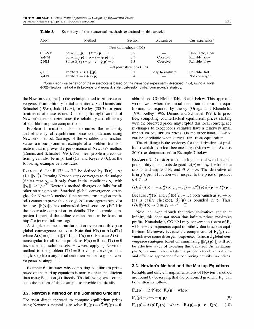
Table 3. Summary of the numerical methods examined in this article.
Abbr. Method Section Advantage Our experiencea
Newton methods (NM)
CG-NM Solve F�4p5= 4 ¶ï º�54p5= 0 3.2 — Unreliable, slowÇ-NM Solve F�4p5= p− c−Ç4p5= 0 3.3 Coercive Reliable, slowÆ-NM Solve F�4p5= p− c− Æ4p5= 0 3.3 Coercive Reliable, slow
Fixed-point iterations (FPI)Æ-FPI Iterate p← c+ Æ4p5 3.4 Easy to evaluate Reliable, fastÇ-FPI Iterate p← c+Ç4p5 3.4 — Not convergent
aConclusions on behavior of these methods is based on the numerical experiments described in §4, using a novelGMRES-Newton method with Levenberg-Marquardt style trust-region global convergence strategy.
the Newton step, and (ii) the technique used to enforce con-vergence from arbitrary initial conditions. See Dennis andSchnabel (1996), Judd (1998), or Kelley (2003) for goodtreatments of these issues. Choosing the right variant ofNewton’s method determines the reliability and efficiencyof equilibrium price computations.
Problem formulation also determines the reliabilityand efficiency of equilibrium price computations usingNewton’s method. Scalings of the variables and functionvalues are one prominent example of a problem transfor-mation that improves the performance of Newton’s method(Dennis and Schnabel 1996). Nonlinear problem precondi-tioning can also be important (Cai and Keyes 2002), as thefollowing example demonstrates.
Example 6. Let F2 �N → �N be defined by F4x5 = x/41+��x��225. Iterating Newton steps converges to the unique(finite) zero x∗ = 0 only from initial conditions x0 with��x0��2 < 1/
√3. Newton’s method diverges or fails for all
other starting points. Standard global convergence strate-gies for Newton’s method (line search, trust region meth-ods) cannot improve this poor global convergence behaviorbecause ��F4x5��2 has unbounded level sets; see §EC.1 inthe electronic companion for details. The electronic com-panion is part of the online version that can be found athttp://or.journal.informs.org/.
A simple nonlinear transformation overcomes this poorglobal convergence behavior. Note that F4x5 = A4x5f4x5where A4x5= 41+��x��225
−1I and f4x5= x. Because A4x5 isnonsingular for all x, the problems F4x5 = 0 and f4x5 = 0have identical solution sets. However, applying Newton’smethod to the problem f4x5 = 0 trivially converges in asingle step from any initial condition without a global con-vergence strategy. �
Example 6 illustrates why computing equilibrium pricesbased on the markup equations is more reliable and efficientthan using Equation (4) directly. The following two sectionsecho the pattern of this example to provide the details.
3.2. Newton’s Method on the Combined Gradient
The most direct approach to compute equilibrium pricesusing Newton’s method is to solve F�4p5 = 4 ¶ï º�54p5 = 0,
abbreviated CG-NM in Table 3 and below. This approachworks well when the initial condition is near an equi-librium, as required by theory (Ortega and Rheinboldt1970, Kelley 1995, Dennis and Schnabel 1996). In prac-tice, computing counterfactual equilibrium prices startingwith the observed prices may exploit this local convergenceif changes to exogeneous variables have a relatively smallimpact on equilibrium prices. On the other hand, CG-NMcan be unreliable when started “far” from equilibrium.
The challenge is the tendency for the derivatives of prof-its to vanish as prices become large (Morrow and Skerlos2010), as demonstrated in Example 7 below.
Example 7. Consider a simple logit model with linear inprice utility and an outside good: u4p5= −�p+v for some� > 0 and any v ∈ �, and � > −�. The derivative offirm f ’s profit function with respect to the price of productk ∈Jf is
4Dk º�f 54p5= −�PLk 4p54pk − ck5+�PL
k 4p5º�f 4p5+PLk 4p50
Because PLk 4p5 and PL
k 4p54pk −ck5 both vanish as pk → �
(as is easily checked), º�f 4p5 is bounded in p. Thus,4Dk º�f 54p5→ 0 as pk → �. �
Note that even though the price derivatives vanish atinfinity, this does not mean that infinite prices maximizeprofits. Nonetheless, CG-NM may converge to a zero of F�
with some components equal to infinity that is not an equi-librium. Moreover, because the components of F�4p5 canvanish over some divergent sequences, standard global con-vergence strategies based on minimizing ��F�4p5��2 will notbe effective ways of avoiding this behavior. As in Exam-ple 6, we must reformulate the problem to obtain reliableand efficient approaches for computing equilibrium prices.
3.3. Newton’s Method and the Markup Equations
Reliable and efficient implementations of Newton’s methodare found by observing that the combined gradient, F� , canbe written as follows:
F�4p5=4 ¶DP54p5>F�4p5 where
F�4p5=p−c−Ç4p5 (9)
F�4p5=å4p5F�4p5 where F�4p5=p−c−Æ4p50 (10)
Morrow and Skerlos: Fixed-Point Approaches to Computing Equilibrium Prices334 Operations Research 59(2), pp. 328–345, © 2011 INFORMS
Either F� or F� can be used to compute simultaneouslystationary prices when 4 ¶DP54p5> and å4p5, respectively,are nonsingular (Morrow and Skerlos 2010). Of course, F�
and F� recast the first-order condition as a fixed-point prob-lem: F� is zero if and only if the BLP-markup equationholds, and F� is zero if and only if the Æ-markup equa-tion holds.
Solving F�4p5= 0 or F�4p5= 0, abbreviated Ç-NM andÆ-NM, respectively, in Table 3 and below, requires the solu-tion of nontrivial nonlinear systems with Newton’s method.Ç-NM and Æ-NM, however, are less likely to have thecomputational problems that CG-NM exhibits because theyexploit norm-coercivity of the maps F� and F� (Morrowand Skerlos 2010). A norm-coercive map has a norm thattends to infinity with the norm of its argument (Ortega andRheinboldt 1970, Harker and Pang 1990). Globally conver-gent implementations of Newton’s method that decrease thevalue of ��F4p5��2 in each step produce bounded sequencesof iterates when F is norm-coercive. Thus, solving the BLP-or Æ-markup equation instead of the literal first-order con-dition removes the tendency for applications of Newton’smethod to compute “spurious” solutions at infinity.
3.4. Fixed-Point Iteration
In addition to applications of Newton’s method, the BLP-and Æ-markup equations suggest applying fixed-point itera-tion to solve for equilibrium prices.
The fixed-point iteration p 7→ c + Æ4p5 based on theÆ-markup equation, here abbreviated Æ-FPI, can efficientlycompute equilibrium prices for some problems. Æ-FPI hasrelatively efficient steps because no linear systems needto be solved, unlike every other method listed in Table 3.Although we are not aware of a general convergence prooffor Æ-FPI, this iteration has converged reliably on test prob-lems including the examples in §§4 and 5 below.
The fixed-point iteration p 7→ c + Ç4p5, abbreviatedÇ-FPI, based on the BLP-markup equation need not con-verge. Example 8 below gives a case in which Ç can failto be even locally convergent.
Example 8. Consider multiproduct monopoly pricing witha simple logit model having uj4p5 = −�p + vj for some� > 0, any vj ∈ �, and � > −�. It is well known thatfor a single-product firm, unique profit-maximizing pricesexist (Anderson and de Palma 1988, Milgrom and Roberts1990, Caplin and Nalebuff 1991). Morrow (2008) provesthat profit-optimal prices p∗ are unique for the multiproductcase—and even so with multiple firms—even though profitsare not quasi-concave (Hanson and Martin 1996).
In this example, Ç-FPI is not always locally conver-gent near p∗, whereas Æ-FPI is always superlinearly locallyconvergent. For an arbitrary continuously differentiablefunction F and p∗ = F4p∗5, F is contractive on some neigh-borhood of p∗ in some norm ��·�� if �44DF54p∗55 < 1where �4A5 (Ortega and Rheinboldt 1970). We show that
�44DÇ54p∗55 > 1 may hold while �44DÆ54p∗55= 0, where�4A5 denotes the spectral radius of the matrix A.
The components of the BLP-markup function Ç aregiven by �k4p5 = �−141 −
∑Jj=1 P
Lj 4p55
−1 for all k. Fromthis formula, the equation
�44DÇ54p∗55=
∑Jj=1 P
Lj 4p∗5
1 −∑J
j=1 PLj 4p∗5
=
J∑
j=1
euj 4pj1∗5−�
can be derived. For valuations of the outside good, � , suffi-ciently close to −�, �44DÇ54p∗55 > 1 can hold; see §EC.2in the e-companion for details.
To prove the claim regarding �44DÆ54p∗55, note that�k4p5= º�4p5+ 1/�, and thus 4Dl�k54p∗5= 4Dl º�54p∗5= 0for all k1 l. �
Even if the BLP-markup equation does generate aconvergent fixed-point iteration, evaluating Ç involves thesolution of F linear systems that grow in size with the num-ber of products offered by the firms. The work requiredto evaluate Ç using a direct method like PLU or QR factor-ization is O46maxf Jf 7
35, given values of P4p5, å4p5, and¶â4p5 as approximated using simulation. The work to eval-uate Æ is only O46maxf Jf 7
25 given P4p5, å4p5, and ¶â4p5(Morrow and Skerlos 2010). Generally speaking, functionevaluations must be cheap for the linear convergence offixed-point iterations to result in faster computations thanthe superlinearly or quadratically convergent variants ofNewton’s method.
3.5. Simulation
In most mixed-logit models, P4p5, å4p5, and ¶â4p5 cannotbe computed exactly because they involve integrals withno closed-form expression (Train 2003). Instead, they areapproximated with sample averages over a finite set of sam-ples from T. This sampling technique, called simulation,is commonly applied in estimation (McFadden 1989, Train2003, Draganska and Jain 2004).
Simulation is applied to compute equilibrium prices byapplying CG-NM, Ç-NM, Æ-NM, and Æ-FPI to the finite-sample simulator defined in Example 4. ApproximatingP4p5, å4p5, and ¶â4p5 (among other quantities) in this waydominates the computational burden of each approach tocomputing equilibrium prices (Morrow and Skerlos 2010).Other sampling techniques such as importance or quasi-random sampling could be employed to reduce this burden(Train 2003). In §4.3 we investigate how the variation incomputed equilibrium prices derived from drawing differ-ent sample sets changes with S, the sample set size.
4. A Numerical ExampleThis section studies a differentiated product market withmany products and a high degree of firm and productheterogeneity: the 2005 new-vehicle market in the UnitedStates. The new-vehicle market has played a significant role
Morrow and Skerlos: Fixed-Point Approaches to Computing Equilibrium PricesOperations Research 59(2), pp. 328–345, © 2011 INFORMS 335
in the development of differentiated product market mod-els based on Bertrand competition. Section 4.1 describestwo models of the vehicle market. Section 4.2 comparesthe methods in Table 3 using these models, and §4.3 inves-tigates the sensitivity of computed equilibrium prices tochoice of initial condition and the sample set.
4.1. Model Description
This section describes the demand models and vehicle dataused in the numerical trials. These models are not intendedto provide an accurate depiction of the new-vehicle marketsuitable for making inferences about firm behavior or con-ducting policy analysis. Rather, these models only providea realistic example of the type of problem that arises inempirical applications.
4.1.1. Two Demand Models. Modified versions of theBoyd and Mellman (1980) model of Example 1 andthe Berry et al. (1995) model of Example 2 character-ize demand for new vehicles. Some vehicle characteris-tics originally included in these models are excluded dueto a lack of data, but the originally estimated coefficientsare used for each characteristic included; see §EC.3.1in the e-companion for details. The modified Boyd andMellman model uses three vehicle characteristics: a met-ric of size, 0–60 acceleration, and fuel consumption. Thecoefficients used are those reported by Boyd and Mellmanand are reproduced here in Table 5. The modified Berryet al. again uses three vehicle characteristics: operatingcost, horsepower-to-weight ratio (a common proxy for 0–60acceleration), and vehicle length times vehicle width. Againthe coefficients used are those reported by Berry et al. andare reproduced here in Table 6. Income 4�5 has a lognor-mal distribution fit to current population survey data from2005 (Berry et al. 1995, Petrin 2002, Berry et al. 2004,CPS 2007). Note that price enters the Boyd and Mellmanmodel in 1980 dollars, whereas price enters the Berry et al.model in 1983 dollars.
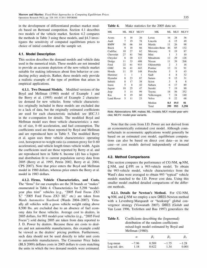
4.1.2. Firms, Vehicle Characteristics, and Costs.The “firms” for our examples are the 38 brands or “makes”enumerated in Table 4. Characteristics for 5,298 “model-year plus trim” vehicles (e.g., “2005 Ford Focus ZX3S,” “2005 Ford Focus ZX3 SE,” etc.) are taken fromWards Automotive Yearbook (Wards 2004–2007). Virtu-ally all vehicles with a gross vehicle weight rating above8,500 lbs. are excluded due to an absence of fuel econ-omy data for these vehicles. Average cost to dealers, in2005 dollars, for 993 model-year vehicles (e.g., “2005 FordFocus”) sold during 2005 are taken from data reported toJ. D. Power by dealers. Because these are costs to deal-ers and not automobile manufacturers, this example couldbe viewed as the dealers’ pricing problem. Furthermore,such data should not be used directly to infer unit coststo automobile manufacturers. The Consumer Price Index(BLS 2009) deflates costs in 2005 dollars to costs matchingthe units in which the two demand models were estimated.
Table 4. Make statistics for the 2005 data set.
MK ML MLY MLYV MK ML MLY MLYV
Acura 6 18 26 Lexus 16 28 36Audi 7 19 78 Lincoln 6 15 49BMW 30 66 84 Mazda 11 26 98Buick 9 18 66 Mercedes-Benz 46 85 132Cadillac 10 27 62 Mercury 9 19 87Chevrolet 27 81 760 Mini 1 3 10Chrysler 8 20 123 Mitsubishi 12 29 128Dodge 11 33 408 Nissan 11 39 268Ford 22 61 933 Oldsmobile 2 3 18GMC 16 41 443 Pontiac 12 31 91Honda 11 35 148 Porsche 3 9 43Hummer 1 1 1 Saab 4 8 32Hyundai 8 23 87 Saturn 9 15 31Infiniti 8 17 38 Scion 3 8 8Isuzu 5 8 42 Subaru 6 17 89Jaguar 10 25 47 Suzuki 7 19 90Jeep 5 14 99 Toyota 18 56 352Kia 8 19 60 Volkswagen 7 24 140Land Rover 5 11 23 Volvo 9 22 68
Median 8.5 19.5 81Total 399 993 5,298
Note. Abbreviations: MK: makes; ML: models; MLY: model-year vehi-cles; MLYV: model-year variants.
Note that the costs from J.D. Power are not derived froman econometrically estimated cost model. Although coun-terfactuals in econometric applications would generally bebased on an estimated cost model, equilibrium computa-tions can also be based on direct cost data—as in ourcase—or cost models derived independently of demandestimation.
4.2. Method Comparisons
This section compares the performance of CG-NM, Ç-NM,Æ-NM, and Æ-FPI on a 993-vehicle model. To obtainthe 993-vehicle model, vehicle characteristics from theWard’s data were averaged to obtain 993 “typical” vehiclemodels matched to the J.D. Power cost data. Using thissmaller model enabled detailed comparisons of the differ-ent methods.
4.2.1. Details for Newton’s Method. For CG-NM,Ç-NM, and Æ-NM we employ a new GMRES-Newton methodwith a Levenberg-Marquardt or “hookstep” global con-vergence strategy (Viswanath 2007). GMRES (Golub andVan Loan 1996, Trefethen and Bau 1997) generalizes the
Table 5. Coefficients describing the (lognormal)distribution of the random coefficientsmixed-logit model estimated by Boyd andMellman (1980).
� �1 �2 �3
Log-mean −7096 00589 −1075 −1028Log-std. dev. 1018 00622 1034 00001
Morrow and Skerlos: Fixed-Point Approaches to Computing Equilibrium Prices336 Operations Research 59(2), pp. 328–345, © 2011 INFORMS
Table 6. Coefficients describing the (normal)distribution of the random coefficientsmixed-logit model estimated by Berry et al.(1995).
� � �1 �2 �3 �0
Mean 430501 10 −00122 30460 20883 −80582Std. dev. 0 1 1005 20056 40628 10794
Note. � is lognormally distributed, and thus reported values are thelog-mean and log-standard deviation.
popular conjugate gradient iterative method for solvingsymmetric linear systems (Judd 1998, Nocedal and Wright2006) to nonlinear systems of equations in which theJacobian 4DF5 is, in general, asymmetric. GMRES-Newtonmethods have been applied to large-scale nonlinear fluiddynamics and radiative transfer problems; see, for exam-ple, Brown and Saad (1990), Eisenstat and Walker (1994),Pernice and Walker (1998), Kelley (2003), Pawlowski et al.(2006, 2008), Viswanath (2009), Viswanath and Cvitanovic(2009), and Halcrow et al. (2009). Viswanath’s approachcombines the GMRES method for solving linear systemswith the Levenberg-Marquardt “hookstep” globalizationstrategy (Levenberg 1944, Marquardt 1963, Dennis andSchnabel 1996). Line search (Dennis and Schnabel 1996)and Powell’s “hybrid” or “dogleg” step (Powell 1970,Dennis and Schnabel 1996) globalization strategies havealso been extended to GMRES-Newton methods; see, e.g.,Brown and Saad (1990), Eisenstat and Walker (1994), Kel-ley (1995), Pernice and Walker (1998), Kelley (2003),Pawlowski et al. (2006, 2008).
Other important details are as follows. The termina-tion condition for all methods is ��4 ¶ï º�54p5��
�¶ 10−6.
Note that this is the natural termination condition forCG-NM, but not the usual termination condition for Ç-NM or Æ-NM (Morrow and Skerlos 2010). The second-order conditions are always checked at computed points.In CG-NM, GMRES uses a point-dependent preconditioner(Morrow and Skerlos 2010), whereas neither Ç-NM orÆ-NM appear to require preconditioning. GMRES is given50 steps to solve the unpreconditioned Newton system to atight relative residual tolerance of 10−6, and GMRES is neverrestarted. Although loosening this relative residual toler-ance (Viswanath 2007) or including adaptive tolerances(Eisenstat and Walker 1996, Pernice and Walker 1998,Kelley 2003) can improve computation speed and reliabil-ity (Tuminaro et al. 2002), we do not feel this will make asignificant impact on our results. In our examples GMRES isalready very fast: generally, fewer than 10 GMRES steps arerequired to achieve convergence to an inexact Newton step,even with the tight relative residual tolerance. AdditionalGMRES steps are cheap relative to the “overhead” require-ment of computing the Jacobian matrices. For CG-NM,these inclusions may have a more pronounced improve-ment in computational times. Finally, a primary benefitfrom GMRES-Newton methods is that they can be built on
evaluations of F alone (Brown and Saad 1990, Pernice andWalker 1998). Using the analytic Jacobians is usually themost efficient approach, and thus the computations belowuse the analytic Jacobians (Morrow and Skerlos 2010).
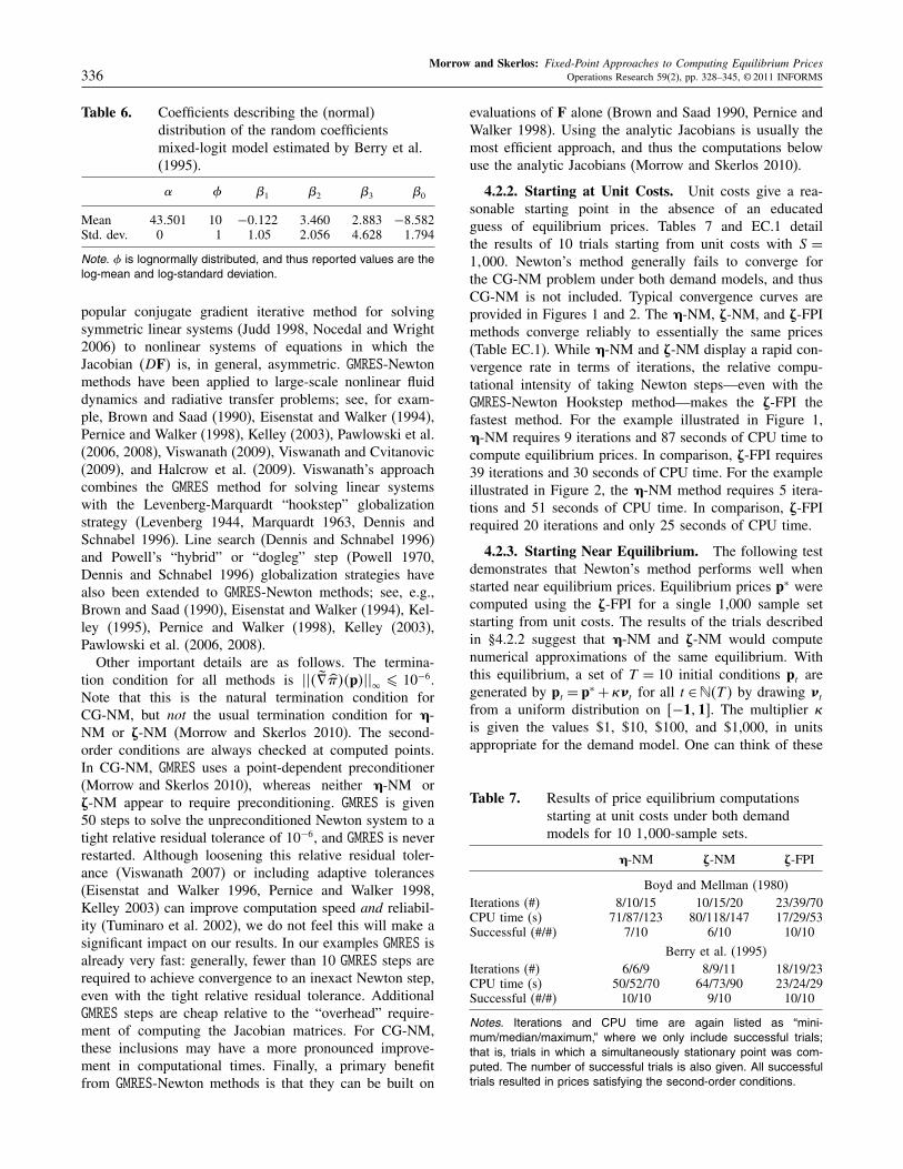
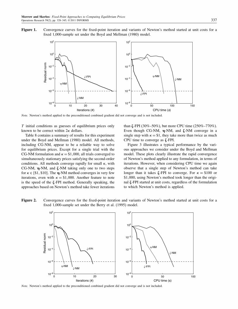
4.2.2. Starting at Unit Costs. Unit costs give a rea-sonable starting point in the absence of an educatedguess of equilibrium prices. Tables 7 and EC.1 detailthe results of 10 trials starting from unit costs with S =
11000. Newton’s method generally fails to converge forthe CG-NM problem under both demand models, and thusCG-NM is not included. Typical convergence curves areprovided in Figures 1 and 2. The Ç-NM, Æ-NM, and Æ-FPImethods converge reliably to essentially the same prices(Table EC.1). While Ç-NM and Æ-NM display a rapid con-vergence rate in terms of iterations, the relative compu-tational intensity of taking Newton steps—even with theGMRES-Newton Hookstep method—makes the Æ-FPI thefastest method. For the example illustrated in Figure 1,Ç-NM requires 9 iterations and 87 seconds of CPU time tocompute equilibrium prices. In comparison, Æ-FPI requires39 iterations and 30 seconds of CPU time. For the exampleillustrated in Figure 2, the Ç-NM method requires 5 itera-tions and 51 seconds of CPU time. In comparison, Æ-FPIrequired 20 iterations and only 25 seconds of CPU time.
4.2.3. Starting Near Equilibrium. The following testdemonstrates that Newton’s method performs well whenstarted near equilibrium prices. Equilibrium prices p∗ werecomputed using the Æ-FPI for a single 1,000 sample setstarting from unit costs. The results of the trials describedin §4.2.2 suggest that Ç-NM and Æ-NM would computenumerical approximations of the same equilibrium. Withthis equilibrium, a set of T = 10 initial conditions pt aregenerated by pt = p∗ + �Ít for all t ∈�4T 5 by drawing Ít
from a uniform distribution on 6−1117. The multiplier �is given the values $1, $10, $100, and $1,000, in unitsappropriate for the demand model. One can think of these
Table 7. Results of price equilibrium computationsstarting at unit costs under both demandmodels for 10 11000-sample sets.
Ç-NM Æ-NM Æ-FPI
Boyd and Mellman (1980)Iterations (#) 8/10/15 10/15/20 23/39/70CPU time (s) 71/87/123 80/118/147 17/29/53Successful (#/#) 7/10 6/10 10/10
Berry et al. (1995)Iterations (#) 6/6/9 8/9/11 18/19/23CPU time (s) 50/52/70 64/73/90 23/24/29Successful (#/#) 10/10 9/10 10/10
Notes. Iterations and CPU time are again listed as “mini-mum/median/maximum,” where we only include successful trials;that is, trials in which a simultaneously stationary point was com-puted. The number of successful trials is also given. All successfultrials resulted in prices satisfying the second-order conditions.
Morrow and Skerlos: Fixed-Point Approaches to Computing Equilibrium PricesOperations Research 59(2), pp. 328–345, © 2011 INFORMS 337
Figure 1. Convergence curves for the fixed-point iteration and variants of Newton’s method started at unit costs for afixed 1,000-sample set under the Boyd and Mellman (1980) model.
0 10 20 30 40 0 50 100 150
�-NM
�-NM
�-FPI �-NM�-NM
�-FPI
100
10–2
10–4
10–6
10–8
102
100
10–2
10–4
10–6
10–8
102
Res
idua
l nor
m
CPU time (s)Iterations (#)
Note. Newton’s method applied to the preconditioned combined gradient did not converge and is not included.
T initial conditions as guesses of equilibrium prices onlyknown to be correct within 2� dollars.
Table 8 contains a summary of results for this experimentunder the Boyd and Mellman (1980) model. All methods,including CG-NM, appear to be a reliable way to solvefor equilibrium prices. Except for a single trial with theCG-NM formulation and �= $11000, all trials converged tosimultaneously stationary prices satisfying the second-orderconditions. All methods converge rapidly for small �, withCG-NM, Ç-NM, and Æ-NM taking only one to two stepsfor � ∈ 8$11$109. The Ç-NM method converges in very fewiterations, even with � = $11000. Another feature to noteis the speed of the Æ-FPI method. Generally speaking, theapproaches based on Newton’s method take fewer iterations
Figure 2. Convergence curves for the fixed-point iteration and variants of Newton’s method started at unit costs for afixed 1,000-sample set under the Berry et al. (1995) model.
0 10 20 30 0 50 100
�-NM
�-NM
�-NM
�-NM
�-FPI
�-FPI
Iterations (#) CPU time (s)
Res
idua
l nor
m
100
10–2
10–4
10–6
10–8
102
100
10–2
10–4
10–6
10–8
102
Note. Newton’s method applied to the preconditioned combined gradient did not converge and is not included.
than Æ-FPI (30%–50%), but more CPU time (250%–770%).Even though CG-NM, Ç-NM, and Æ-NM converge in asingle step with �= $1, they take more than twice as muchCPU time to converge as Æ-FPI.
Figure 3 illustrates a typical performance by the vari-ous approaches we consider under the Boyd and Mellmanmodel. These plots clearly illustrate the rapid convergenceof Newton’s method applied to any formulation, in terms ofiterations. However, when considering CPU time we againobserve that a single step of Newton’s method can takelonger than it takes Æ-FPI to converge. For � = $100 or$11000, using Newton’s method took longer than the origi-nal Æ-FPI started at unit costs, regardless of the formulationto which Newton’s method is applied.
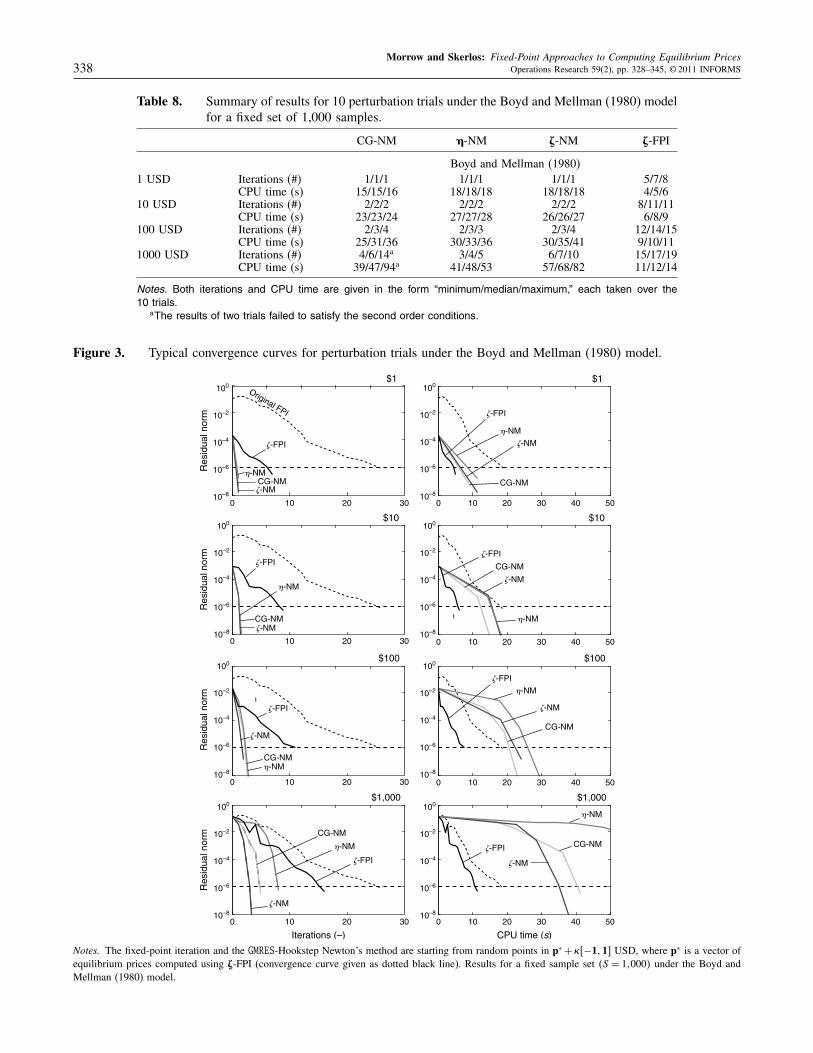
Morrow and Skerlos: Fixed-Point Approaches to Computing Equilibrium Prices338 Operations Research 59(2), pp. 328–345, © 2011 INFORMS
Table 8. Summary of results for 10 perturbation trials under the Boyd and Mellman (1980) modelfor a fixed set of 1,000 samples.
CG-NM Ç-NM Æ-NM Æ-FPI
Boyd and Mellman (1980)1 USD Iterations (#) 1/1/1 1/1/1 1/1/1 5/7/8
CPU time (s) 15/15/16 18/18/18 18/18/18 4/5/610 USD Iterations (#) 2/2/2 2/2/2 2/2/2 8/11/11
CPU time (s) 23/23/24 27/27/28 26/26/27 6/8/9100 USD Iterations (#) 2/3/4 2/3/3 2/3/4 12/14/15
CPU time (s) 25/31/36 30/33/36 30/35/41 9/10/111000 USD Iterations (#) 4/6/14a 3/4/5 6/7/10 15/17/19
CPU time (s) 39/47/94a 41/48/53 57/68/82 11/12/14
Notes. Both iterations and CPU time are given in the form “minimum/median/maximum,” each taken over the10 trials.
aThe results of two trials failed to satisfy the second order conditions.
Figure 3. Typical convergence curves for perturbation trials under the Boyd and Mellman (1980) model.
$1
$10
$100
100
10–2
10–4
10–6
10–8
100
10–2
10–4
10–6
10–8
Iterations (–) CPU time (s)
$1,000
0 10 20 30
0 10 20 30
0 10 20 30
0 10 20 30
0 10 20 30 40 50
0 10 20 30 40 50
0 10 20 30 40 50
0 10 20 30 40 50
$1,000
$100
$10
$1
�-FPI
�-FPI
�-FPI�-FPI
�-FPI
�-FPI
�-FPI
�-FPI
�-NM
�-NM
�-NM
�-NM�-NM
�-NM
�-NM
�-NM
�-NM
�-NM
�-NM
�-NM
�-NM
�-NM
�-NM
�-NM
CG-NM
CG-NM
CG-NM
CG-NM
CG-NM
CG-NM
CG-NMCG-NM
ı
ı
Original FPI
Res
idua
l nor
m
100
10–2
10–4
10–6
10–8
100
10–2
10–4
10–6
10–8
Res
idua
l nor
m
100
10–2
10–4
10–6
10–8
Res
idua
l nor
m
100
10–2
10–4
10–6
10–8
Res
idua
l nor
m
100
10–2
10–4
10–6
10–8
100
10–2
10–4
10–6
10–8
Notes. The fixed-point iteration and the GMRES-Hookstep Newton’s method are starting from random points in p∗ +�6−1117 USD, where p∗ is a vector ofequilibrium prices computed using Æ-FPI (convergence curve given as dotted black line). Results for a fixed sample set 4S = 110005 under the Boyd andMellman (1980) model.
Morrow and Skerlos: Fixed-Point Approaches to Computing Equilibrium PricesOperations Research 59(2), pp. 328–345, © 2011 INFORMS 339
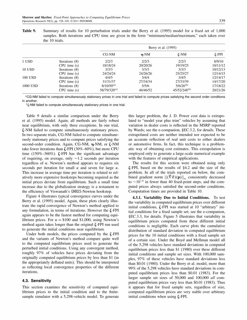
Table 9. Summary of results for 10 perturbation trials under the Berry et al. (1995) model for a fixed set of 1,000samples. Both iterations and CPU time are given in the form “minimum/median/maximum,” each taken overthe 10 trials.
Berry et al. (1995)
CG-NM Ç-NM Æ-NM Æ-FPI
1 USD Iterations (#) 2/2/3 2/2/3 2/2/3 8/9/10CPU time (s) 18/18/24 20/20/26 19/19/25 10/11/12
10 USD Iterations (#) 3/3/3 3/3/3 3/3/3 10/12/13CPU time (s) 24/24/24 24/26/26 25/25/27 12/14/15
100 USD Iterations (#) 4/4/5 3/4/4 3/4/5 12/14/17CPU time (s) 31/31/37 27/34/34 27/33/39 14/17/20
1000 USD Iterations (#) 8/10/504a5 5/5/6 5/6/264b5 17/18/22CPU time (s) 58/79/3204a5 46/46/52 45/52/2484b5 20/21/26
aCG-NM failed to compute simultaneously stationary prices in one trial and failed to compute prices satisfying the second order conditionsin another.
bÆ-NM failed to compute simultaneously stationary prices in one trial.
Table 9 details a similar comparison under the Berryet al. (1995) model. Again, all methods are fairly robustnear equilibrium, with only three exceptions. In one trial,Æ-NM failed to compute simultaneously stationary prices.In two separate trials, CG-NM failed to compute simultane-ously stationary prices and to compute prices satisfying thesecond-order condition. Again, CG-NM, Ç-NM, or Æ-NMtake fewer iterations than Æ-FPI (30%–60%), but more CPUtime (150%–360%). Æ-FPI has the significant advantageof requiring, on average, only ∼1.2 seconds per iterationregardless of �. Newton’s method appears to requires sixseconds per iteration for small � and seven for large �.This increase in average time per iteration is related to rel-atively more expensive hooksteps becoming required as theinitial prices deviate from equilibrium. Such a small timeincrease due to the globalization strategy is a testament tothe efficiency of Viswanath’s GMRES-Newton hookstep.
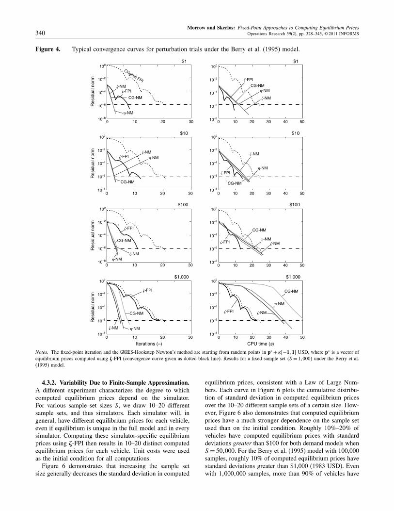
Figure 4 illustrates typical convergence curves under theBerry et al. (1995) model. Again, these plots clearly illus-trate the rapid convergence of Newton’s method applied toany formulation, in terms of iterations. However the Æ-FPIagain appears to be the fastest method for computing equi-librium prices. For � = $100 and $1,000, using Newton’smethod again takes longer than the original Æ-FPI run usedto generate the initial conditions near equilibrium.
Under both models, the prices computed by the Æ-FPIand the variants of Newton’s method compare quite wellto the computed equilibrium prices used to generate theperturbed initial conditions. Using any convergent method,roughly 97% of vehicles have prices deviating from theoriginally computed equilibrium prices by less than $1 (inthe appropriately deflated units). This should be interpretedas reflecting local convergence properties of the differentiterations.
4.3. Sensitivity
This section examines the sensitivity of computed equi-librium prices to the initial condition and to the finite-sample simulator with a 5,298-vehicle model. To generate
this larger problem, the J. D. Power cost data is extrapo-lated to “model year plus trim” vehicles by assuming thatvariation in dealer costs is reflected in the MSRP reportedby Wards; see the e-companion, §EC.3.2, for details. Theseextrapolated costs are neither intended nor expected to bean accurate reflection of real unit costs to either dealersor automotive firms. In fact, this technique is a problem-atic way of obtaining cost estimates. This extrapolation isemployed only to generate a large-scale numerical examplewith the features of empirical applications.
The results for this section were obtained using onlyÆ-FPI, based on the results of §4.2 and the size of theproblem. In all of the trials reported on below, the com-bined gradient norm ��4 ¶ï º�54p5��
�consistently decreased
to ∼10−6 in fewer than 40 fixed-point steps, and the com-puted prices always satisfied the second-order conditions.Computation times are provided in Table 10.
4.3.1. Variability Due to Initial Conditions. To testthe variability in computed equilibrium prices over differentinitial conditions, Æ-FPI was started at 10 “arbitrary” ini-tial conditions for a fixed sample set; see the e-companion,§EC.3.3, for details. Figure 5 illustrates that variability inequilibrium prices computed from these different initialconditions is negligible. Each curve plots the cumulativedistribution of standard deviation in computed equilibriumprices for the 10 initial conditions with a fixed sample setof a certain size. Under the Boyd and Mellman model allof the 5,298 vehicles have standard deviations in computedequilibrium prices less than $1 (1980) over these differentinitial conditions and sample set sizes. With 100,000 sam-ples, 97% of these vehicles have standard deviations lessthan $0.01 (1980). Under the Berry et al. model, more than99% of the 5,298 vehicles have standard deviations in com-puted equilibrium prices less than $0.01 (1983). For thelarger sample set sizes of 50,000 and 100,000 all com-puted equilibrium prices vary less than $0.01 (1983). Thusit appears that for fixed sample sets, regardless of size,computed equilibrium prices are very stable over arbitraryinitial conditions when using Æ-FPI.
Morrow and Skerlos: Fixed-Point Approaches to Computing Equilibrium Prices340 Operations Research 59(2), pp. 328–345, © 2011 INFORMS
Figure 4. Typical convergence curves for perturbation trials under the Berry et al. (1995) model.
$1
$10
$100
100
10–2
10–4
10–6
10–8
100
10–2
10–4
10–6
10–8
Iterations (–) CPU time (s)
$1,000
0 10 20 30
0 10 20 30
0 10 20 30
0 10 20 30
0 10 20 30 40 50
0 10 20 30 40 50
0 10 20 30 40 50
0 10 20 30 40 50
$1,000
$100
$10
$1
�-FPI
�-FPI
�-FPI
�-FPI
�-FPI
�-FPI
�-FPI
�-FPI
�-NM
�-NM
�-NM�-NM
�-NM
�-NM
�-NM
�-NM
�-NM
�-NM
�-NM
�-NM
�-NM
�-NM
�-NM
�-NM
CG-NM
CG-NM
CG-NM CG-NM
CG-NM
CG-NM
CG-NM
CG-NM
ı
ı
Original FPI
Res
idua
l nor
m
100
10–2
10–4
10–6
10–8
100
10–2
10–4
10–6
10–8
Res
idua
l nor
m
100
10–2
10–4
10–6
10–8
Res
idua
l nor
m
100
10–2
10–4
10–6
10–8
Res
idua
l nor
m
100
10–2
10–4
10–6
10–8
100
10–2
10–4
10–6
10–8
Notes. The fixed-point iteration and the GMRES-Hookstep Newton’s method are starting from random points in p∗ +�6−1117 USD, where p∗ is a vector ofequilibrium prices computed using Æ-FPI (convergence curve given as dotted black line). Results for a fixed sample set 4S = 110005 under the Berry et al.(1995) model.
4.3.2. Variability Due to Finite-Sample Approximation.A different experiment characterizes the degree to whichcomputed equilibrium prices depend on the simulator.For various sample set sizes S, we draw 10–20 differentsample sets, and thus simulators. Each simulator will, ingeneral, have different equilibrium prices for each vehicle,even if equilibrium is unique in the full model and in everysimulator. Computing these simulator-specific equilibriumprices using Æ-FPI then results in 10–20 distinct computedequilibrium prices for each vehicle. Unit costs were usedas the initial condition for all computations.
Figure 6 demonstrates that increasing the sample setsize generally decreases the standard deviation in computed
equilibrium prices, consistent with a Law of Large Num-bers. Each curve in Figure 6 plots the cumulative distribu-tion of standard deviation in computed equilibrium pricesover the 10–20 different sample sets of a certain size. How-ever, Figure 6 also demonstrates that computed equilibriumprices have a much stronger dependence on the sample setused than on the initial condition. Roughly 10%–20% ofvehicles have computed equilibrium prices with standarddeviations greater than $100 for both demand models whenS = 501000. For the Berry et al. (1995) model with 100,000samples, roughly 10% of computed equilibrium prices havestandard deviations greater than $1,000 (1983 USD). Evenwith 110001000 samples, more than 90% of vehicles have
Morrow and Skerlos: Fixed-Point Approaches to Computing Equilibrium PricesOperations Research 59(2), pp. 328–345, © 2011 INFORMS 341
Table 10. Longest observed computation times forvarious sample set sizes using Æ-FPI.
Boyd and Berry et al.Mellman (1980) (1995)
Number ofsamples (#) 103 104 105 106 103 104 105 106
CPU time (hrs) 001 204 404 65 002 104 705 125
standard deviations in computed equilibrium prices greaterthan $1 (1983, USD).
These results suggest that practitioners must be careful toensure that the conclusions of counterfactual experimentsare not influenced by variations in computed equilibriumprices due to simulation.
5. Multiple EquilibriaThe uniqueness of equilibrium—or lack thereof—is ofcentral relevance to economic applications of equilibrium
Figure 5. Cumulative distribution of standard deviation in computed equilibrium prices over 10 random initial conditionsfor several sample set sizes (given in the numeric labels) under the Boyd and Mellman (1980) and Berry et al.(1995) models.
1.0
0.8
0.6
0.4
0.9
0.7
0.5
0.3
0.2
0.1
0.0
Boyd and Mellman (1980)
Standard deviation (1980 USD)
Fra
ctio
n of
veh
icle
s (–
)
100 102 10410–4 10–210–6 100 102 10410–4 10–210–6
Initi
al c
ondi
tions
1,000
5,000 10,000
100,000
50,000
1.0
0.8
0.6
0.4
0.9
0.7
0.5
0.3
0.2
0.1
0.0
Standard deviation (1983 USD)
Fra
ctio
n of
veh
icle
s (–
)
Initi
alco
nditi
ons
1,000
5,000
10,000
100,000
50,000
Berry et al. (1995)
Figure 6. Cumulative distribution of standard deviation in computed equilibrium prices over 10–20 sample sets of severalsizes (given in the numeric labels) under the Boyd and Mellman (1980) and Berry et al. (1995) models.
1.0
0.9
0.8
0.7
0.6
0.5
0.4
0.3
0.2
0.1
0.0
Standard deviation (1983 USD)
Fra
ctio
n of
veh
icle
s
50
100
500
5,000
50,000
1,000
10,000
100,000
1,000,000
50
100
50050,000
10,000
100,000
1,000,000
10–1 100 101 102 103 104 10510–2 10–1 100 101 102 103 104 10510–2
1.0
0.9
0.8
0.7
0.6
0.5
0.4
0.3
0.2
0.1
0.0
Standard deviation (1980 USD)
Fra
ctio
n of
veh
icle
s
5,0001,000
models. When equilibrium is not unique, it is not nec-essarily clear what behavior the model prescribes. Manyfinite-action games such as entry/exit games have multi-ple equilibria (Bresnahan and Reiss 1991b, a; Berry andReiss 2007). This phenomenon is not unique to discreteaction games and can occur in Bertrand competition mod-els as well. Determining the uniqueness and/or multiplicityof Bertrand-Nash equilibrium prices with nonlinear utili-ties, heterogeneous multiproduct firms, and heterogeneousindividuals is currently an open problem deserving furtheranalysis.
Although computational methods currently enable theuse of large-scale equilibrium models of differentiatedproduct markets, they offer little to the rigorous inves-tigation of the uniqueness or multiplicity of equilibriumin Bertrand competition. Because the strategy spaces forBertrand competition are uncountable, computational meth-ods can only be employed to determine what equilib-ria might exist rather than determine their uniqueness or
Morrow and Skerlos: Fixed-Point Approaches to Computing Equilibrium Prices342 Operations Research 59(2), pp. 328–345, © 2011 INFORMS
multiplicity. On the other hand, computational methodscurrently provide the only means for practitioners to under-stand what equilibria might exist for empirical Bertrandcompetition models.
Newton’s method has a very important property—localconvergence (Ortega and Rheinboldt 1970, Dennis andSchnabel 1996)—that will influence the performance ofÇ-NM and Æ-NM when there are multiple equilibria.Specifically, Newton’s method will converge to any vec-tor of simultaneously stationary prices when started nearenough to these prices. Because of local convergence,computational exploration with Ç-NM and/or Æ-NM canrecover any simultaneously stationary prices, and thus anylocal equilibrium. However, one can never know with cer-tainty that all simultaneously stationary prices have beencomputed when using computational methods alone. Fur-thermore, as mentioned in §2.3, not every vector of simulta-neously stationary prices is necessarily a local equilibrium.Thus, Newton’s method can converge to “solutions” that arenot local equilibria. Thus, whereas Newton’s method hasthe significant advantage of being theoretically guaranteedto compute any simultaneously stationary point, exploringfor multiple equilibria in large-scale examples with Ç-NMor Æ-NM could be a time-consuming exercise.
Unlike Newton’s method, fixed-point iteration is not nec-essarily locally convergent if the fixed-point map is notlocally contractive. This is illustrated by the followingexample.
Example 9. The map f 4x5 = x2 has two fixed points:0 and 1. Fixed-point iteration converges to 0 starting atany x ∈ 4−1115, converges to 1 if started in 8±19, andconverges to +� if started in 4−�1−15 ∪ 411�5. Thus,fixed-point iteration cannot converge to 1 when started atany x 6= 1 near 1. �
The lack of even local convergence of fixed-point itera-tions suggests that Æ-FPI should be adopted with caution insituations where there might be multiple equilibria. How-ever, the performance of fixed-point iteration is very prob-lem specific. Example 10 below shows that it is possiblefor Æ-FPI to effectively compute equilibrium prices, evenwhen there multiple equilibria, and simultaneously, station-ary prices that are not equilibria.
Example 10. Consider two firms, each offering a single,“branded” product. Firms 1 and 2 offer products 1 and 2,respectively, at the same unit cost, c1 = 001 = c2. Thereare three “types” of customers. Individuals of types 1 and2 are price sensitive, but “brand-loyal” in the sense thatindividuals of type 1 have a higher valuation for product 1than product 2, and vice versa for consumers of type 2.Individuals of type 3 are “brand-indifferent” and choosebetween products 1 and 2 based only on price. Set T =
8112139 and let the systematic utilities be
u14�1p5= −�4�5p+ v14�5
u24�1p5= −�4�5p+ v24�5
�4�5= 0 with
�415= 10 v1415= 0 v2415= −1
�425= 10 v1425= −1 v2425= 0
�435= 1 v1435= 0 v2435= 00
The relative frequencies of types in the population are�415= 0045, �425= 0045, and �435= 001.
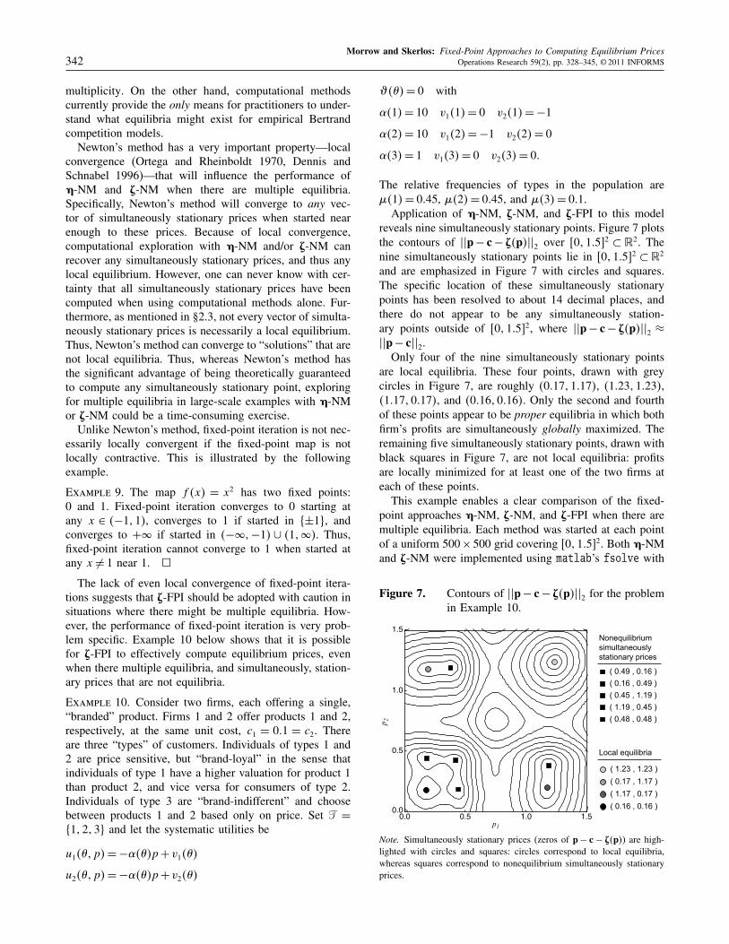
Application of Ç-NM, Æ-NM, and Æ-FPI to this modelreveals nine simultaneously stationary points. Figure 7 plotsthe contours of ��p− c− Æ4p5��2 over 60110572 ⊂ �2. Thenine simultaneously stationary points lie in 60110572 ⊂ �2
and are emphasized in Figure 7 with circles and squares.The specific location of these simultaneously stationarypoints has been resolved to about 14 decimal places, andthere do not appear to be any simultaneously station-ary points outside of 60110572, where ��p− c− Æ4p5��2 ≈
��p− c��2.Only four of the nine simultaneously stationary points
are local equilibria. These four points, drawn with greycircles in Figure 7, are roughly 40017110175, 41023110235,41017100175, and 40016100165. Only the second and fourthof these points appear to be proper equilibria in which bothfirm’s profits are simultaneously globally maximized. Theremaining five simultaneously stationary points, drawn withblack squares in Figure 7, are not local equilibria: profitsare locally minimized for at least one of the two firms ateach of these points.
This example enables a clear comparison of the fixed-point approaches Ç-NM, Æ-NM, and Æ-FPI when there aremultiple equilibria. Each method was started at each pointof a uniform 500 ×500 grid covering 60110572. Both Ç-NMand Æ-NM were implemented using matlab’s fsolve with
Figure 7. Contours of ��p− c− Æ4p5��2 for the problemin Example 10.
Local equilibria
Nonequilibriumsimultaneouslystationary prices
( 0.49 , 0.16 )
( 0.16 , 0.49 )
( 0.45 , 1.19 )
( 1.19 , 0.45 )
( 0.48 , 0.48 )
p1
0.0 0.5 1.0 1.50.0
0.5
1.0
1.5
p 2
( 0.17 , 1.17 )
( 1.23 , 1.23 )
( 0.16 , 0.16 )
( 1.17 , 0.17 )
Note. Simultaneously stationary prices (zeros of p− c − Æ4p5) are high-lighted with circles and squares: circles correspond to local equilibria,whereas squares correspond to nonequilibrium simultaneously stationaryprices.
Morrow and Skerlos: Fixed-Point Approaches to Computing Equilibrium PricesOperations Research 59(2), pp. 328–345, © 2011 INFORMS 343
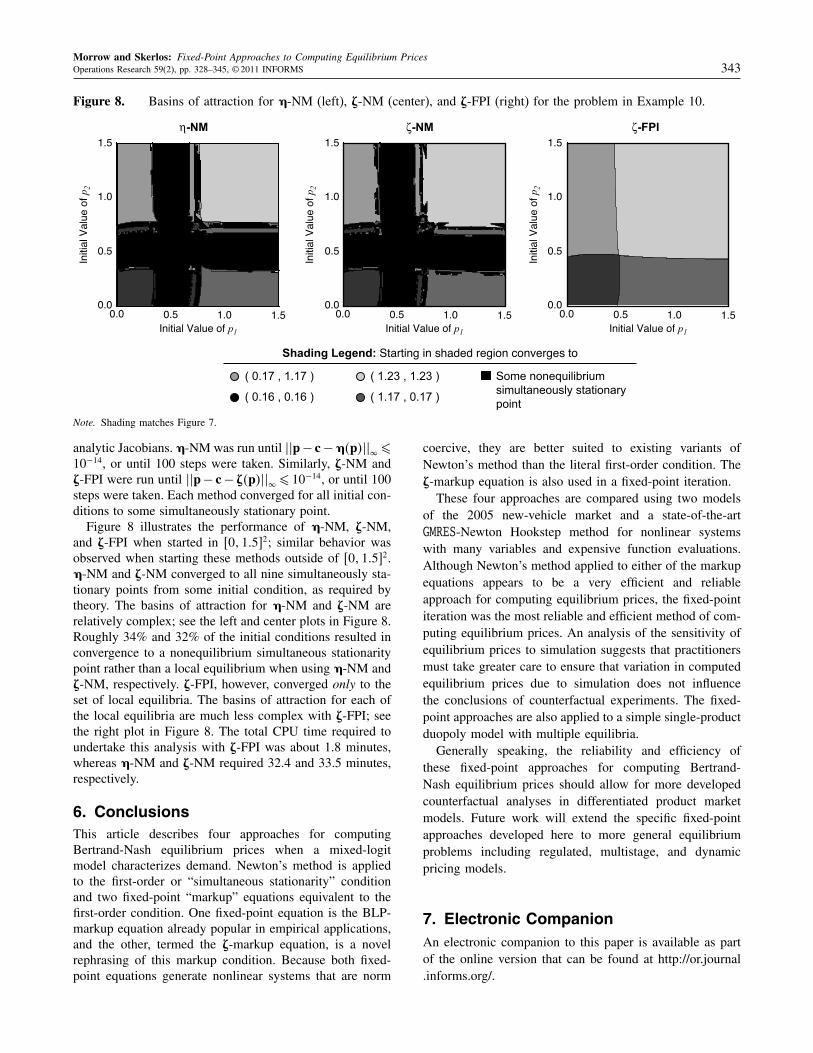
Figure 8. Basins of attraction for Ç-NM (left), Æ-NM (center), and Æ-FPI (right) for the problem in Example 10.
0.0
0.5
1.0
1.5
Initial Value of p1
Initi
al V
alue
of p2
0.0 0.5 1.0 1.5
1
0.0
0.5
1.0
1.5
0.0 0.5 1.0 1.5Initial Value of p
Initi
al V
alue
of p2
Shading Legend: Starting in shaded region converges to
Some nonequilibriumsimultaneously stationarypoint
( 0.17 , 1.17 ) ( 1.23 , 1.23 )
( 0.16 , 0.16 ) ( 1.17 , 0.17 )
0.0
0.5
1.0
1.5
Initial Value of p1
Initi
al V
alue
of p2
0.0 0.5 1.0 1.5
η-NM ζ-NM ζ-FPI
Note. Shading matches Figure 7.
analytic Jacobians. Ç-NM was run until ��p− c−Ç4p5���¶
10−14, or until 100 steps were taken. Similarly, Æ-NM andÆ-FPI were run until ��p− c− Æ4p5��
�¶ 10−14, or until 100
steps were taken. Each method converged for all initial con-ditions to some simultaneously stationary point.
Figure 8 illustrates the performance of Ç-NM, Æ-NM,and Æ-FPI when started in 60110572; similar behavior wasobserved when starting these methods outside of 60110572.Ç-NM and Æ-NM converged to all nine simultaneously sta-tionary points from some initial condition, as required bytheory. The basins of attraction for Ç-NM and Æ-NM arerelatively complex; see the left and center plots in Figure 8.Roughly 34% and 32% of the initial conditions resulted inconvergence to a nonequilibrium simultaneous stationaritypoint rather than a local equilibrium when using Ç-NM andÆ-NM, respectively. Æ-FPI, however, converged only to theset of local equilibria. The basins of attraction for each ofthe local equilibria are much less complex with Æ-FPI; seethe right plot in Figure 8. The total CPU time required toundertake this analysis with Æ-FPI was about 1.8 minutes,whereas Ç-NM and Æ-NM required 32.4 and 33.5 minutes,respectively.
6. ConclusionsThis article describes four approaches for computingBertrand-Nash equilibrium prices when a mixed-logitmodel characterizes demand. Newton’s method is appliedto the first-order or “simultaneous stationarity” conditionand two fixed-point “markup” equations equivalent to thefirst-order condition. One fixed-point equation is the BLP-markup equation already popular in empirical applications,and the other, termed the Æ-markup equation, is a novelrephrasing of this markup condition. Because both fixed-point equations generate nonlinear systems that are norm
coercive, they are better suited to existing variants ofNewton’s method than the literal first-order condition. TheÆ-markup equation is also used in a fixed-point iteration.
These four approaches are compared using two modelsof the 2005 new-vehicle market and a state-of-the-artGMRES-Newton Hookstep method for nonlinear systemswith many variables and expensive function evaluations.Although Newton’s method applied to either of the markupequations appears to be a very efficient and reliableapproach for computing equilibrium prices, the fixed-pointiteration was the most reliable and efficient method of com-puting equilibrium prices. An analysis of the sensitivity ofequilibrium prices to simulation suggests that practitionersmust take greater care to ensure that variation in computedequilibrium prices due to simulation does not influencethe conclusions of counterfactual experiments. The fixed-point approaches are also applied to a simple single-productduopoly model with multiple equilibria.
Generally speaking, the reliability and efficiency ofthese fixed-point approaches for computing Bertrand-Nash equilibrium prices should allow for more developedcounterfactual analyses in differentiated product marketmodels. Future work will extend the specific fixed-pointapproaches developed here to more general equilibriumproblems including regulated, multistage, and dynamicpricing models.
7. Electronic CompanionAn electronic companion to this paper is available as partof the online version that can be found at http://or.journal.informs.org/.
Morrow and Skerlos: Fixed-Point Approaches to Computing Equilibrium Prices344 Operations Research 59(2), pp. 328–345, © 2011 INFORMS
AcknowledgmentsThis research was supported by the National Science Foun-dation, the University of Michigan Transportation ResearchInstitute’s Doctoral Studies Program, and a research fel-lowship at the Belfer Center for Science and Interna-tional Affairs at the Harvard Kennedy School. Both authorswish to thank Walter McManus, Brock Palen, DivakarViswanath, and Erin MacDonald. They also acknowledgehelpful suggestions offered by Fred Feinberg, John Hauser,Meredith Fowlie, Kenneth Judd, and the support of KellySims-Gallagher and Henry Lee at the Belfer Center. Threeanonymous reviewers and the editorial staff at OperationsResearch also provided valuable input.
ReferencesAnderson, S. P., A. de Palma. 1988. Spatial price discrimination with
heterogeneous products. Rev. Econom. Stud. 55(4) 573–592.Anderson, S. P., A. de Palma. 1992. The logit as a model of product
differentiation. Oxford Econom. Papers 44(1) 51–67.Austin, D., T. Dinan. 2005. Clearing the air: The costs and consequences
of higher CAFE standards and increased gasoline taxes. J. Environ.Econom. Management 50 562–582.
Baye, M. R., D. Kovenock. 2008. Bertrand competition. S. N. Durlaf,L. E. Blume, eds. The New Palgrave Dictionary of Economics, 2nded. Palgrave Macmillian, London.
Bento, A. M., L. M. Goulder, E. Henry, M. R. Jacobsen, R. H. von Haefen.2005. Distributional and efficiency impacts of gasoline taxes: Aneconometrically based multi-market study. Amer. Econom. Rev. 95(2)282–287.
Beresteanu, A., S. Li. 2008. Gasoline prices, government support, andthe demand for hybrid vehicles in the U.S. Working paper, DukeUniversity, Durham, NC.
Berry, S., P. Reiss. 2007. Empirical models of entry and market structure.M. Armstrong, R. Porter, eds. Handbook of Industrial Organization,Chapter 29, Vol. 3. Elsevier, Amsterdam.
Berry, S., J. Levinsohn, A. Pakes. 1995. Automobile prices in marketequilibrium. Econometrica 63(4) 841–890.
Berry, S., J. Levinsohn, A. Pakes. 2004. Differentiated products demandsystems from a combination of micro and macro data: The new carmarket. J. Political Econom. 112(1) 68–105.
Boyd, J. H., R. E. Mellman. 1980. The effect of fuel economy standardson the U.S. automotive market: An hedonic demand analysis. Trans-portation Res. A 14A 367–378.
Bresnahan, T. F., P. C. Reiss. 1991a. Empirical models of discrete games.J. Econometrics 48(1–2) 57–81.
Bresnahan, T. F., P. C. Reiss. 1991b. Entry and competition in concentratedmarkets. J. Political Econom. 99(5) 977–1009.
Brown, P. N., Y. Saad. 1990. Hybrid Krylov methods for nonlinear systemsof equations. SIAM J. Sci. Statist. Comput. 11(3) 450–481.
Bureau of Labor Statistics (BLS). 2009. Consumer price index. AccessedApril 24, 2009, http://www.bls.gov/cpi/.
Cai, X.-C., D. E. Keyes. 2002. Nonlinearly preconditioned inexact Newtonalgorithms. SIAM J. Sci. Statist. Comput. 24(1) 183–200.
Caplin, A., B. Nalebuff. 1991. Aggregation and imperfect competition:On the existence of equilibrium. Econometrica 59(1) 25–59.
CBO. 2003. The economic costs of fuel economy standards versusa gasoline tax. Technical report, Congressional Budget Office,Washington, DC.
Choi, S. C., W. S. Desarbo, P. T. Harker. 1990. Product positioning underprice competition. Management Sci. 36(2) 175–199.
CPS. 2007. Current population survey. Accessed December 31, 2007,http://www.census.gov/cps/.
Dennis, J. E., R. B. Schnabel. 1996. Numerical Methods for Uncon-strained Optimization and Nonlinear Equations, Society for Indus-trial and Applied Mathematics, Philadelphia.
Doraszelski, U., M. Draganska. 2006. Market segmentation strategies ofmultiproduct firms. J. Indust. Econom. 54(1) 125–149.
Draganska, M., D. Jain. 2004. A likelihood approach to estimating marketequilibrium models. Management Sci. 50(5) 605–616.
Dube, J.-P., J. T. Fox, C.-L. Su. 2011. Improving the performance ofBLP static and dynamic discrete choice random coefficients demandestimation. Working paper, University of Chicago, Chicago.
Dube, J.-P., P. Chintagunta, A. Petrin, B. Bronnenberg, R. Goettler, P. B.Seetharaman, K. Sudhir, R. Thomadsen, Y. Zhao. 2002. Structuralapplications of the discrete choice model. Marketing Lett. 13(3)207–220.
Eisenstat, S. C., H. F. Walker. 1994. Globally convergent inexact Newtonmethods. SIAM J. Optim. 4(2) 393–422.
Eisenstat, S. C., H. F. Walker. 1996. Choosing the forcing terms in aninexact Newton method. SIAM J. Sci. Comput. 17(1) 16–32.
Ferris, M. C., J.-S. Pang. 1997. Engineering and economic applications ofcomplementarity problems. SIAM Rev. 39(4) 669–713.
Goldberg, P. K. 1995. Product differentiation and oligopoly in interna-tional markets: The case of the U.S. automobile industry. Economet-rica 63(4) 891–951.
Goldberg, P. K. 1998. The effects of the corporate average fuel efficiencystandards in the U.S. J. Indust. Econom. 46(1) 1–33.
Golub, G. H., C. F. Van Loan. 1996. Matrix Computations. The JohnsHopkins University Press, Baltimore.
Goolsbee, A., A. Petrin. 2004. The consumer gains from direct broadcastsatellites and the competition with cable TV. Econometrica 72(2)351–381.
Halcrow, J., J. F. Gibson, P. Cvitanovic, D. Viswanath. 2009. Heteroclinicconnections in plane Couette flow. J. Fluid Mechanics 611 365–376.
Hanson, W., K. Martin. 1996. Optimizing multinomial logit profit func-tions. Management Sci. 42(7) 992–1003.
Harker, P. T., J.-S. Pang. 1990. Finite-dimensional variational inequalityand nonlinear complementarity problems: A survey of theory, algo-rithms, and applications. Math. Programming 48(1–3) 161–220.
Jacobsen, M. R. 2006. Evaluating U.S. fuel economy standards in a modelwith producer and household heterogeneity. Working paper, StanfordUniversity, Stanford, CA.
Judd, K. L. 1998. Numerical Methods in Economics. MIT Press,Cambridge, MA.
Kelley, C. T. 1995. Iterative Methods for Linear and Nonlinear Equations,Frontiers in Applied Mathematics, Vol. 16. Society for Industrial andApplied Mathematics, Philadelphia.
Kelley, C. T. 2003. Solving Nonlinear Equations with Newton’s Method.Fundamentals of Algorithms. Society for Industrial and AppliedMathematics, Philadelphia.
Knittel, C. R., K. Metaxoglou. 2008. Estimation of random coefficientdemand models: Challenges, difficulties, and warnings. Workingpaper, University of California, Davis, Davis.
Levenberg, K. 1944. A method for the solution of certain non-linear prob-lems in least squares. Quart. J. Appl. Math. 2 164–168.
Marquardt, D. 1963. An algorithm for least-squares estimation of nonlin-ear parameters. SIAM J. Appl. Math. 11(2) 431–441.
McFadden, D. L. 1989. A method of simulated moments for estimation ofdiscrete response models without numerical integration. Economet-rica 57(5) 995–1026.
McFadden, D., K. Train. 2000. Mixed MNL models for discrete response.J. Appl. Econometrics 15(5) 447–470.
Michalek, J. J., P. Y. Papalambros, S. J. Skerlos. 2004. A study of fuelefficiency and emission policy impact on optimal vehicle design deci-sions. J. Mech. Design 126(6) 1062–1070.
Milgrom, P., J. Roberts. 1990. Rationalizability, learning, and equilib-rium in games with strategic complementarities. Econometrica 58(6)1255–1277.
Morrow, W. R. 2008. A fixed-point approach to equilibrium pricing in dif-ferentiated product markets. Ph.D. thesis, Department of MechanicalEngineering, University of Michigan, Ann Arbor.
Morrow, W. R., S. J. Skerlos. 2010. Fixed-point approaches to com-puting Bertrand-Nash equilibrium prices under mixed-logit demand:A framework for analysis and efficient computational methods. Tech-nical report, Iowa State University, Ames.
Morrow and Skerlos: Fixed-Point Approaches to Computing Equilibrium PricesOperations Research 59(2), pp. 328–345, © 2011 INFORMS 345
Nevo, A. 1997. Mergers with differentiated products: The case ofthe ready-to-eat cereal industry. Technical report, University ofCalifornia, Berkeley, Berkeley.
Nevo, A. 2000a. Mergers with differentiated products: The case of theready-to-eat cereal industry. RAND J. Econom. 31(3) 395–421.
Nevo, A. 2000b. A practitioner’s guide to estimation of random-coefficients logit models of demand. J. Econom. Management Strat-egy 9(4) 513–548.
Nocedal, J., S. J. Wright. 2006. Numerical Optimization, 2nd ed. Springer-Verlag, New York.
Ortega, J. M., W. C. Rheinboldt. 1970. Iterative Solution of NonlinearEquations in Several Variables. Society for Industrial and AppliedMathematics, Philadelphia.
Pawlowski, R. P., J. N. Shadid, J. P. Simonis, H. F. Walker. 2006. Glob-alization techniques for Newton-Krylov methods and applications tothe fully coupled solutions of the Navier-Stokes equations. SIAM Rev.48(4) 700–721.
Pawlowski, R. P., J. P. Simonis, H. F. Walker, J. N. Shadid. 2008. InexactNewton dogleg methods. SIAM J. Numer. Anal. 46(4) 2112–2132.
Pernice, M., H. F. Walker. 1998. NITSOL: A Newton iterative solver fornonlinear systems. SIAM J. Sci. Comput. 19(1) 302–318.
Petrin, A. 2002. Quantifying the benefits of new products: The case of theminivan. J. Political Econom. 110(4) 705–729.
Powell, M. J. D. 1970. A hybrid method for nonlinear equations.P. Rabinowitz, ed. Numerical Methods for Nonlinear AlgebraicEquations, Chapter 6. Gordon and Breach Science Publishers,New York, 87–114.
Schmedders, K. 2008. Numerical optimization methods in economics.S. N. Durlaf, L. E. Blume, eds. The New Palgrave Dictionary ofEconomics, 2nd ed. Palgrave Macmillian, London.
Smith, H. 2004. Supermarket choice and supermarket competition in mar-ket equilibrium. Rev. Econom. Stud. 71 235–263.
Su, C.-L., K. L. Judd. 2008. Constrained optimization approaches to esti-mation of structural models. Working paper, University of Chicago,Chicago.
Thomadsen, R. 2005. The effect of ownership structure on pricesin geographically differentiated markets. RAND J. Econom. 36(4)908–929.
Train, K. 2003. Discrete Choice Methods with Simulation. CambridgeUniversity Press, Cambridge, UK.
Trefethen, L. N., D. Bau. 1997. Numerical Linear Algebra. Society forIndustrial and Applied Mathematics, Philadelphia.
Tuminaro, R. S., H. F. Walker, J. N. Shadid. 2002. On backtracking failurein Newton-GMRES methods with a demonstration for the Navier-Stokes equations. J. Comput. Phys. 180(2) 549–558.
Viswanath, D. 2007. Recurrent motions within plane Couette turbulence.J. Fluid Mechanics 580 339–358.
Viswanath, D. 2009. The critical layer in pipe flow at high Reynoldsnumber. Philos. Trans. Royal Soc. 367 561–576.
Viswanath, D., P. Cvitanovic. 2009. Stable manifolds and the transition toturbulence in pipe flow. J. Fluid Mechanics 627 215–233.
Wards. 2004–2007. Wards Automotive Yearbooks. Wards Reports Inc.,Southfield, MI.