The ‘center of excellence’ FIW (http://www.fiw.ac.at/), is a project of WIFO, wiiw, WSR and Vienna University of Economics and Business, University of Vienna, Johannes Kepler University Linz on behalf of the BMWFW.

FIW – Working Paper

Remittances, finance and growth: does financial development foster remittances and their impact

on economic growth?*

Izabela Sobiech1

In this paper, I measure the importance of remittances and financial development for developing countries. I estimate an index of overall financial conditions and use it to determine the relevance of the financial sector as a transmission channel for remittances to affect economic growth. The index brings together information from existing measures, reflecting size, depth and efficiency of the financial sector. It is created by means of an unobserved components model. I show that the more financial development in a country, the smaller becomes the impact of remittances on economic growth and it can even turn negative. For countries with weaker financial markets there is a positive effect, but significant only at the earliest stages of financial development. The effect becomes negative in the third quartile of financial development. These results hold irrespective of the measure of financial development included, but are most profound in case of the created index. This means that estimates based on proxies might be slightly biased. I also show that countries with both low levels of remittances and financial development should first focus on developing the latter, while migrants' transfers become important for growth if the country has a moderate level of financial development. JEL: F24, O11, O15 and O16 Keywords: remittances, economic growth, financial development, unobserved

components model, dynamic panel data analysis

1 Goethe University Frankfurt and Technische Universität Darmstadt. Address : Theodor-W.-Adorno Platz 3,

60323 Frankfurt, Germany. E-mail : izabela.sobiech@hof.uni-frankfurt.de

Abstract

The author

FIW Working Paper N° 158 October 2015

Remittances, finance and growth: does financial

development foster remittances and their impact on

economic growth?∗

Izabela Sobiech†

This version: September 19, 2015

Abstract

In this paper, I measure the importance of remittances and financial development

for developing countries. I estimate an index of overall financial conditions and

use it to determine the relevance of the financial sector as a transmission channel

for remittances to affect economic growth. The index brings together information

from existing measures, reflecting size, depth and efficiency of the financial sector.

It is created by means of an unobserved components model. I show that the more

financial development in a country, the smaller becomes the impact of remittances

on economic growth and it can even turn negative. For countries with weaker

financial markets there is a positive effect, but significant only at the earliest stages of

financial development. The effect becomes negative in the third quartile of financial

development. These results hold irrespective of the measure of financial development

included, but are most profound in case of the created index. This means that

estimates based on proxies might be slightly biased. I also show that countries

with both low levels of remittances and financial development should first focus on

developing the latter, while migrants’ transfers become important for growth if the

country has a moderate level of financial development.

JEL classification: F24, O11, O15 and O16

Keywords: remittances, economic growth, financial development, unobserved

components model, dynamic panel data analysis.

∗I thank Michael Binder, Philipp Harms, Mauro Rodrigues Jr., Volker Nitsch and the participantsof the GSEFM Summer Institute, XV Conference on International Economics, Money and Macro BrownBag Seminar at Goethe University and of the 21st International Panel Data Conference for their helpfulcomments. Responsibility for all remaining errors rests with the author.

†Goethe University Frankfurt and Technische Universitaet Darmstadt. Address: Theodor-W.-AdornoPlatz 3, 60323 Frankfurt, Germany, izabela.sobiech@hof.uni-frankfurt.de

1 Introduction

Remittances are migrants’ transfers in money and kind sent to relatives in their home

countries. According to the World Bank Migration and Remittances Team, in 2012-2014

75% of the value of all such transfers were received by developing countries, either from

industrial economies (North-South, ca. 53%) or from other developing countries (South-

South, for example from Russia to Ukraine or India to Bangladesh). In the last 15 years

these flows have been increasing rapidly, exceeding official development assistance (ODA),

and more steadily than foreign direct investment flows (FDI) (cf. Fig. 1). Economists have

become interested in these international money flows, as an important source of development

financing.

Remittances have been recently debated in the context of the post-2015 Sustainable

Development Agenda of the United Nations Development Programme (UNDP, Agenda to

be adopted in September 2015). There are 17 newly proposed Sustainable Development

Goals (SDGs) and their achievement relies on public as well as private financing from

industrial countries. Remittances have been recognized as one of potential sources of

funding for the SDGs during the UN Third International Conference on Financing for

Development in Addis Ababa in July 2015:1

“40. We recognize the positive contribution of migrants for inclusive growth and sus-

tainable development in countries of origin [. . . ]. Remittances from migrant workers,

[. . . ], are typically wages transferred to families, primarily to meet part of the needs

of the recipient households. They cannot be equated to other international financial

flows, such as foreign direct investment, ODA or other public sources of financing for

development. We will work to ensure that adequate and affordable financial services

are available to migrants and their families in both home and host countries.[. . . ]

We will support national authorities to address the most significant obstacles to the

continued flow of remittances, such as the trend of banks withdrawing services, to

work towards access to remittance transfer services across borders. [. . . ] including

by promoting competitive and transparent market conditions. We will exploit new

technologies, promote financial literacy and inclusion, and improve data collection.”

This paragraph from the Addis Ababa conference Action Agenda recognized the role

of remittances in supporting families in developing countries and emphasizes that financial

sector development is necessary to boost migrants’ transfers through lower costs and better

service availability. Fostering remittances and the financial/banking sector as a transmission

channel can therefore have short-run and long-run effects on economic development of

receiving countries.

In this paper I evaluate the impact of remittances on economic growth, taking into

account financial sector development measured with a newly constructed index. There

1Resolution adopted by the General Assembly on 27 July 2015, Sixty-ninth session, Agenda item 18,UN. http : //www.un.org/ga/search/viewdoc.asp?symbol = A/RES/69/313 accessed August 27, 2015.

1

are several challenges associated with answering this question, in particular with respect

to capturing financial sector development in a comprehensive way, considering its size,

depth and efficiency at the same time. For many developing countries (according to World

Bank’s classification of countries) data on financial indicators2 are generally available only

for short time periods or with gaps. There is also no consensus as for an adequate measure

of financial development – in a related study Giuliano and Ruiz-Arranz (2009) used four

different proxies: deposit to GDP ratio, loan to GDP ratio, credit to GDP ratio and M2 to

GDP ratio to provide some insight about different aspects of financial sector development.3

All of them refer only to the size of the financial sector, therefore Bettin and Zazzaro (2012)

used also a measure of bank inefficiency, but due to data availability their sample is limited

to the time period from 1991 to 2005, not capturing long-run trends.

For these reasons it is worthwhile to create a measure of financial development which

would capture more aspects of the financial sector, helping to evaluate the impact of remit-

tances on growth and the role of the financial intermediaries in this process. In this paper

I tackle this problem by using an unobserved components model in which a financial devel-

opment indicator is extracted from available information stemming from existing measures

describing the size, depth and efficiency of the financial sector, combined into one number.

The measure proposed in this paper can provide information about the overall impact of

financial sector development on the remittance-growth relationship. By combining elements

of size and efficiency of the financial sector, it takes into account the fact that availability

of credit in the economy is determined both by bank efficiency (bureaucracy related to the

application and decision process) and by availability of financial resources. The proposed

measure assigns lower values of financial development to countries who have high deposits

or credit to GDP ratio but inefficient banks and non-banking institutions. Similarly in the

opposite situation, the score of countries with very high efficiency but low size proxies is

also adjusted downwards. The first case allows to control for loans which were not given

out for the most productive use, and the second case accounts for the fact that even if

procedures related to obtaining a loan are simple, applicants may not be able to receive

financial support due to unavailability of financial resources.

The main purpose of this paper is therefore to verify whether size or efficiency mat-

ter more – does the “overall financial development” strengthen the effect of remittances

on economic growth in transfer-receiving developing countries (positive coefficient on the

remttance-finance interaction term) or is it a substitute to remittances, removing credit

constraints, providing financial resources for productive activities and allowing transfer re-

cipients to spend remittances in a different, non-growth enhancing way (negative impact of

the remittance-finance interaction term on GDP per capita growth)?

2for example in the Financial Structure Dataset.3In his study for Ghana, Adenutsi (2011) provides a broader list with potential measures of financial

development, including additionally: stock price index or market capitalization index, level of nominalinterest rates, real interest rate growth, bank credit to the private sector to private deposits ratio, spreadbetween deposit and lending rate, and others.

2

Another issue pertaining to this research question, and to growth regressions in general,

is the potential endogeneity of financial development measures and remittances (and other

potential determinants of long-run economic growth). In this paper I rely on the assumption

of weak exogeneity of the variables of interest. I account for it by lagging the regressors by

one year with respect to the dependent variable when forming 5-year averages. Then I use

two estimation methods, consistent under this assumption. The quasi-maximum likelihood

for dynamic panel data with fixed effects (QML-FE) is the first method applied and I

discuss the results of it in more detail, as the preferred ones. The advantage of QML-

FE is that, in contrary to GMM methods, it is not necessary to use any instruments and

weak instrument problems described by Roodman (2009) and Bazzi and Clemens (2013)

are avoided. Taking these disadvantages into account, I also apply system GMM estimation

where I use lagged values as internal instruments for all regressors. The second method is

more popular in the literature and can also be seen as a robustness check if my explanatory

variables do not fulfill the exogeneity requirement. Moreover, to remove most common

sources of cross-sectional dependence, time dummies are included in all regressions.

The results of this paper show that the impact of remittances on economic growth in-

deed depends on the level of financial development. For countries with the least advanced

financial sectors there is evidence for positive correlation between remittances and growth,

but the effect turns negative with increasing financial development and migrants’ transfers

can become irrelevant. A country could also experience long-run output losses if it achieved

very high levels of financial development. This means, that remittances and financial de-

velopment can be seen as substitutes. Nonetheless, some initial financial development is an

important prerequisite to induce economic development and to foster remittances. The re-

sults do not change significantly when years 2007-2010 (global financial crisis and following

economic slowdown in industrial countries) are excluded from the sample, preserving the

negative sign of the remittance-finance interaction term in my growth regressions.

The structure of the paper is following: after a brief literature review in Section 2,

Section 3 gives a detailed description of the data used for the creation of the index and for

estimation, Section 4 includes a brief overview of the methodology applied, both for the

index formation and for growth regressions. In Section 5 I present the results concerning

the financial development index and in Section 6 the results of the growth model for a

large cross-section of countries over the time period 1970-2010. All regressions are repeated

for four different measures of financial development, first the overall financial conditions

index and then for some of the variables which were used for its formulation. I control

for measures of investment, government expenditure and human capital. Section 6 includes

also two counterfactual scenarios, firstly of the impact on economic growth if remittances or

financial development remained constant at their initial level for each country, and secondly

if they grew more than in reality – by 20% for each country. Section 7 shows that no strong

structural shifts took place during the financial crisis so that the role of the financial sector

as a substitute for remittances has remained unchanged. Section 8 concludes.

3

2 Related literature

There is a vast literature on the importance of remittances for development and poverty

alleviation, especially for small countries where the ratio of remittances to GDP is high,

reaching more than 30% (for example in Lesotho – with the average ratio over 50%, Moldova,

Tajikistan, Tonga, Samoa4). Given these large numbers, sometimes even bigger than the

value of foreign direct investment (FDI) or official development assistance (ODA), many

researchers have examined the impact of these transfers on economic growth in receiving

countries. Although no consensus has been reached until now, remittances are generally

believed to enhance economic growth through indirect channels (mainly through invest-

ment and human capital formation). Yet, studies focusing on their direct impact on gross

domestic product (GDP) per capita growth5 suggest a negative or at best insignificant re-

lationship (Chami, Fullenkamp, and Jahjah (2003); Gapen, Chami, Montiel, Barajas, and

Fullenkamp (2009); Rao and Hassan (2011)).

Rao and Hassan (2012) and Senbeta (2013) show that the direct effect of remittances

on economic growth may be nil but these transfers still can affect GDP per capita through

different channels: investment, financial development, output volatility, total factor produc-

tivity (TFP) and the real exchange rate. However, on aggregate the effects can cancel out.

Senbeta (2013) argues additionally that the negligible remittance impact on TFP justifies

the lack of significance of migrants’ transfers6 on long-run economic growth. More recently,

Clemens and McKenzie (2014) have shown that the rapid increase in remittances recorded

after the year 2000 is due to changes in the definition of the transfers rather than actual

increases in transfers. In this context, they do not expect remittance measures based on

Balance of Payments data to show significant growth-enhancing effects.

Some studies have found positive causal links between remittances and growth (The

World Bank (2006); Giuliano and Ruiz-Arranz (2009); Catrinescu, Leon-Ledesma, Piracha,

and Quillin (2009); Ramirez and Sharma (2009); Ramirez (2013)7). Giuliano and Ruiz-

Arranz (2009) show that remittances can significantly improve economic growth, if the

financial sector development is taken into account, hence showing that financial sector can

be a channel through which remittances affect growth. They also argue that migrants’

transfers and the financial sector can be substitutes – their growth model includes an

interaction term between the two variables and this term has a negative coefficient, as

4Data sources are described in Section 35In these studies, estimation equations include measures of investment and human capital in order to

partial out the indirect effects of remittances through these channels.6In this paper I use the term migrants’ transfers interchangeably with remittances or remittance inflows.

Until 2009, migrants’ transfers constituted one item in the Balance of Payments, and together with withcompensation of employees added up to remittances. According to International Monetary Fund (2009a)the former was changed into personal transfers, therefore I treat migrants’ transfers and remittances assynonyms (both including also compensation of employees.

7The last two studies consider only selected Latin American and Carribean countries from 1990 to2005/7. The methodology applied therein (fully-modified OLS) was criticized by Gapen et al. (2009) forlimited small sample performance.

4

expected by the authors. They interpret this result as follows. If the financial sector is

well developed, credit constraints are removed and remittances received from relatives from

abroad need not be used in a productive way. However in countries with poorly developed

financial markets remittances can be an important source of financing growth-enhancing

activities.

In the conclusions Giuliano and Ruiz-Arranz (2009) express their concern that the results

might suffer from bias, related in particular to the omission of measures of institutional

quality. Catrinescu et al. (2009) estimate dynamic panel data models including workers’

remittances, various measures of institutional quality8 and interaction terms of the two and

show that better quality of institutions strengthens the impact of remittances on economic

growth. The direct effect of migrants’ transfers however is not robust, and only significantly

positive in some of the specifications.

The substitutability found by Giuliano and Ruiz-Arranz (2009) is confirmed by stud-

ies focused on Latin American and Caribbean countries by Ramirez and Sharma (2009);

Ramirez (2013) and on a larger set of countries by Gapen et al. (2009). However Nya-

mongo, Misati, Kipyegon, and Ndirangu (2012) and Zouheir and Sghaier (2014) provide

evidence of the opposite relationship between remittances and financial development in

African countries. In this region, the two variables seem to be complements with continu-

ing financial deepening strengthening the positive impact of remittances on growth, rather

than mitigating it. As remittances can be deposited in banks, they bring a larger share

of the population in contact with the financial sector, expanding the availability of credit

and savings products (International Monetary Fund (2005); Aggarwal, Demirguc-Kunt, and

Perıa (2011)).

Moreover, countries with underdeveloped financial markets have larger transaction fees

and migrants tend to use informal channels instead (e.g. hawala in parts of Asia and

Africa). Freund and Spatafora (2005) estimate that official remittance data underrates

their value by 35 to 75% which means that the true impact of such transfers on GDP

might still be understated, and these authors also show that lowering transaction costs by

1 percentage point would lead to remittance increasing by 14-23%. This view is supported

e.g. by Ratha (2003):

“By strengthening financial-sector infrastructure and facilitating international travel,

countries could increase remittance flows, thereby bringing more funds into formal

channels.” (p. 157).

Bettin and Zazzaro (2012) explain that the negative sign of the interaction term between

remittances and financial development need not necessarily indicate that these two are

substitutes and can be considered as alternative sources of financing productive investment

for economic growth. They explain, following Rioja and Valev (2004) and Gapen et al.

8They use Corruption Perceptions Index from Transparency International and political risk indicatorsfrom the International Country Risk Guide.

5

(2009), that this coefficient may capture a nonlinear effect of the size of financial sector on

output growth. This is in line with an alternative interpretation of the interaction term

between remittances and financial sector development, focused on the marginal effect of

the latter rather than that of migrants’ transfers. In this case, the negative sign of the

interaction term coefficient can mean that growing remittances increase bank deposits and

available credit but loans are not necessarily given in an efficient way. Therefore, this

remittance-driven rise in the financial sector size does not contribute to economic growth.

For this reason, Bettin and Zazzaro (2012) construct a measure of financial development

related to its (in)efficiency rather than its size and provide evidence for remittances and

financial sector’s efficiency to act as complements for economic prosperity. The efficiency

of the financial sector in a given country is measured as the weighted average of the ratio

of banks’ operating expenses to their net interest revenues and other income.9 Higher

outcomes are related to less efficient financial intermediation. Bettin and Zazzaro (2012)

show that the combined effect of remittances on GDP per capita is lower the larger the size

of the financial sector (substitutes) but it is higher the more efficient the financial sector is

(complements).

3 Data issues

3.1 Remittance data

As mentioned before, the reliability of remittance data is limited. At global level,

receipts of remittances exceed their payments and this discrepancy is growing over time,

see International Monetary Fund (2009b). This is a problem especially in least developed

countries where differences in costs between sending monies through the banking sector

as compared to informal channels are large (and, moreover, transfers in-kind or carrying

cash across borders is very popular). Improving the quality of the data (e.g. by estimating

informal flows from transaction fees or errors and omissions post in the balance of payments)

is beyond the scope of this paper.

Remittance data constitute part of the balance of payments published by the IMF. They

are compiled from different positions in the current and capital account, according to Dilip

Ratha’s recommendation and to the latest Balance of Payments Manual (Ratha (2003),

International Monetary Fund (2009a)). Personal remittances are the sum of three elements:

personal current and capital transfers between resident and nonresident households and

compensation of employees, less taxes and social contributions.10) These data are readily

available in shares of current GDP values in the World Development Indicators data set of

the World Bank. As it is also the most complete compilation, I used it in this paper.

Given the definition of remittances in the Balance of Payments, it is crucial to emphasize

9The data covers 53,820 banks in 66 developing countries over the time period 1990-2005.10For a technical definition of remittances and their computation see International Monetary Fund (2009a)

6

what kinds of transfers are reflected in official statistics, as this can potentially translate

into the direction of their impact on economic growth. Migrants transfer parts of their

income back home for two main reasons: altruistic and selfish – the “portfolio motive” (see

for example Schiopu and Siegfried (2006), Bouhga-Hagbe (2004)). The former is related

to supporting family members who stayed in the home country, mainly in times of bad

economic conditions (countercyclical behavior), while the latter is motivated by portfolio

diversification reasons (procyclical). The first kind of transfers is usually part of remit-

tances, although it depends on the amount sent – some countries set up thresholds below

which transactions are not recorded. The second one should not be included in official

remittance statistics (for example if the money is transferred to the migrant’s own account

– as bank deposits or investments – or if real estate is acquired at home) it should be

booked in the financial account instead. However, this is ambiguous. If relatives in the

home country can withdraw money from the migrant’s account, these cash withdrawals

can be viewed as remittances again. Therefore, in principle, remittances data should only

reflect altruistic transfers, implying that migrants’ transfers could possibly lower economic

growth through real exchange rate appreciation and resource reallocation from tradable

goods to non-tradable goods production – similar to the Dutch disease, cf. Acosta, Lartey,

and Mandelman (2009). However, as these monies can be spent on investment in education

or health care, or in starting a business, it may also generate long-run growth. This paper

tries to evaluate which motive dominates by quantifying growth effects of remittances.

As the official remittance data reflect different kinds of transfers, including both con-

sumption and investment expenditure, different models exist, explaining the direction of

the impact of remittances on GDP. On one hand, Chami et al. (2003) claim that the con-

sumption purpose dominates.11 In their model, moral hazard problems occur and family

members at home lower their labor supply. This effect more than offsets the multiplier

effects from increased consumption leading to negative growth impacts of the transfers. On

the other hand, Giuliano and Ruiz-Arranz (2009) provide a model where resources from

migrants are spent on productive investment and growth impact is positive (also Freund

and Spatafora (2008)). Some authors point out strong altruistic motives and negligible

self-interest portfolio motives, cf. Bouhga-Hagbe (2004) and Schiopu and Siegfried (2006),

while others show an inverted-U relationship between remittances and GDP in the home

economy and positive dependence on the domestic interest rate, cf. Adams (2009).

Until now, no possibility of disentangling the transfers related to each motive has been

proposed for a broad range of countries.12 There is evidence from gravity models suggest-

11They motivate this claim by results of previous empirical studies and by their first-stage regressionresults showing that remittances are significantly correlated with GDP differentials but not with interestrate differentials between the home country and the U.S. (2SLS instrumenting remittances with the twoaforementioned variables)

12For Sub-Saharan countries, Arezki and Brueckner (2012) use rainfall as an instrument for GDP todisentangle the altruistic motive and check whether it is a significant determinant of remittances. Theyalso show that this motive plays an important role when financial development is low – remittances mayhelp overcome domestic credit constraints and take advantage of unexploited investment opportunities.

7

ing that the two motives combined explain less than half of the transfer flows and more

than 50% is generated by links between the sending and receiving countries (distance, com-

mon language, common history; see e.g. Lueth and Ruiz-Arranz (2006) or Balli, Guven,

Gounder, and Ozer-Balli (2010)), which means that separating the altruistic motive from

the portfolio motive, and ignoring the other factors affecting remittance flows at the macro

level, would lead to a substantial underestimation of the total value of the transfers. For

this reason it is also difficult to draw conclusions as for what should be the overall impact

of remittances on economic growth. This is one drawback of large cross-country studies

with aggregate remittance data. Nevertheless, I would expect positive effects in the longer

term, as there is some evidence for such relationships in the literature, when financial sector

development is controlled for (with some measure).

3.2 Data on financial development and the composition of the

index

The main purpose of the financial sector can be summarized as follows:

• “The role of the financial system is to transform liquid, short-term savings into rel-

atively illiquid, long-term investments, thus promoting capital accumulation.” (The

Wold Bank (2005), p.22)

• “Financial markets have an important role in channeling investment capital to its

highest value use.” (Huang (2011))

There is no composite measure which would perfectly gauge the ability of the financial

sector to transform savings into investments. However, such an indicator can be obtained

by combining information from various existing measures. Data on financial development

used in this paper come mostly from the World Bank’s “A Database on Financial Devel-

opment and Structure” (updated in November 2013).This data set covers 203 jurisdictions

over the time period 1960 - 2011. Some variables come from the World Bank’s World

Development Indicators (WDI) database. The following variables have been chosen to

form the financial indicator (classification and definitions from The Wold Bank (2005)):

1. overall size of the financial system:

• financial system deposits to GDP ratio (%) - deposits in deposit money banks

and other financial institutions as a share of GDP

• liquid liabilities to GDP ratio (%) - defined as M3 to GDP ratio, used when

deposits to GDP ratio not available (it is broader than M2 as it includes money

deposits apart from cash, and therefore reflects better the ability of an economy

to channel funds from savers to borrowers). The advantage of this measure is its

broad availability, but it includes M2, therefore may be driven by factors other

than financial depth and reflect more the ability of the system to merely provide

transaction services, see Khan and Senhadji (2000).

8

2. financial institution depth (other than in 1): provision of credit to the economy

• private credit by deposit money banks and other financial institutions to GDP

ratio (%) - all loans offered by commercial banks and other financial institutions

• domestic credit to the private sector to GDP ratio (%) - only domestic loans to

the private sector (both measures from WDI)

3. institutional efficiency - ability of the financial sector to provide high-quality prod-

ucts and services at the lowest cost

• interest rate spread - difference between the lending and the deposit interest rate

(reflects the value of loan-loss provisions and the risk premium associated with

loans to high-risk borrowers)

• deposit interest rate (%)

• overhead costs to total assets (%) - total costs of financial intermediation, in-

cluding operating costs, taxes, loan-loss provisions, net profits, etc.

A measure created based on information from these three categories is able to combine

both size and efficiency aspects of the financial sector, therefore passing the critique raised

by Gapen et al. (2009) and Bettin and Zazzaro (2012) that most studies only focus on

measures of size of the financial sector, ignoring its efficiency. If this measure of overall

financial development is used, concerns related to the interaction term between finance

and remittances reflecting non-linear effects of the size of financial sector increasing with

growing migrants’ transfers are limited. As a measure of “overall financial conditions”, this

index also accounts for the fact that high bank efficiency may not be enough for a liquid

financial sector, if availability of financial resources is limited (small size of the financial

sector).

There is one aspect that is not considered by the constructed index. This measure cap-

tures the ability of the financial sector to transform liquid deposits into illiquid investments,

but it does not capture advantages in terms of risk sharing, allowing for consumption and

output smoothing. This is a feature of all proxies of financial development commonly used

in the remittance-growth relationship literature. Remittances can serve to buffer economic

fluctuations, therefore substituting for this role of the financial sector. However, in this

paper I focus on growth effects, rather than on smoothing, related to second moments,

which constitutes a different research question.

The financial development index (and some of the other proxies listed above) enter my

growth regressions, together with remittance inflows to GDP ratio, an interaction term

between the two, and other determinants of long-run economic development.

3.3 Other determinants of economic growth

Other variables included in the estimations are standard in the growth literature and in-

clude measures of: investment, government expenditure, trade openness, population growth

9

and human capital. Most data come from the World Development Indicators (version 2014)

database of the World Bank: gross fixed capital formation to GDP ratio, government ex-

penditure to GDP ratio, population size and trade openness (exports+imports to GDP

ratio). Human capital is measured by the average years of secondary schooling attained

by the population aged 25 and over (from the Barro and Lee (2013) database, updated in

June 2014).

3.4 Estimation sample

The estimation sample consists of developing countries based on the classification used

by the IMF.13 The maximum time period is 1970-2010, non-overlapping 5-year time averages

for each country are used in the estimations. This means that up to 8 observations are

available per country. Given that remittance to GDP ratios are particularly high in smaller

countries, I did not exclude them from the sample, hence not following the study of Mankiw,

Romer, and Weil (1992). I also keep oil-producers. This should not affect the results to

a large extent, since I identified only 5 countries as small (with average population below

1 million): Barbados, Belize, Cyprus, Fiji, Malta and Swaziland and 2 as oil-producing:

Gabon and Iran, in the set of 61 developing countries. In principle, potential differences

in the structure of these economies should be captured by the individual effects.14 For

former communist countries (Central and Eastern European countries, as well as former

USSR republics) only data from 1990 onward are considered (allowing for a maximum of

4 observations per country, from 1995 to 2010). The list of countries and years for which

data is available is provided in appendix A.1.

4 Methodology

4.1 Dynamic factor model – construction of the financial devel-

opment index

The variables described in Section 3.2 have been grouped into three categories in order

to extract the overall, unobserved financial sector indicator (in what follows also referred

to as overall financial development or overall financial conditions index) from them. I only

include a given country in the sample if data from at least two out of the three categories

are available for at least 20 time periods (not necessarily consecutive). The model is

formalized as follows, following Stock and Watson (1991):

13All developing countries are assigned to one of the following regions: Central and Eastern Europe,Commonwealth of Independent States, developing Asia, Latin America and the Caribbean, Middle Eastand North Africa and Sub-Saharan Africa)

14Mankiw et al. (1992) did not use panel data techniques, therefore were not able to account for potentialstructural differences between oil-producers and other countries. Individual effects included in my fixedeffects regressions do capture these particularities under the assumption that they are time invariant.

10

zit = α+ βιfindevit +wit (1)

findevit = γfindevi,t−1 + vit (2)

with

E(wit) = 0 ∀i, t

E(witwis′) =

{Σ if t=s

0 otherwise

E(vit) = 0, E(v2it) = 1 ∀i, t

where zit is a ki × 1 vector consisting of measures of financial development from the three

categories described in Section 3.2 (ki = 3 if all three measures are available for a country i

at time t, otherwise ki ∈ {0, 1, 2}); findevit is a scalar representing the unobserved financial

sector development measure for country i at time period t and wit is the idiosyncratic error.

ι is a vector of ones with the same dimension as the data in zit (ki × 1). t in this setup

refers to a 1-year time period (in the latter growth regressions it will stand for 5-year time

averages). α is a ki × 1 vector of constants, and β is a ki × ki matrix with off-diagonal

elements equal to zero. Only elements (1,1), (2,2) and (3,3) are estimated and referred to

as β(1), β(2) and β(3).

Equation (1) is referred to as the “measurement equation” (or observation equation).

For each country it is a system of ki equations relating the unobserved overall financial

conditions index to existing proxies of financial development (from the available categories).

Equation (2) is the “state equation”, describing the data generating process which the

created index is assumed to have. In this case both groups of equations (referring to

measured and unobserved variables) are estimated jointly for all countries (parameters

are not country-specific) by maximum likelihood (MLE) and the Kalman Filter.15 This

specification is based on the assumption that existing measures of financial development

are determined by the overall state of the financial development which is unobserved and

that the relationship is the same in all countries. The unobserved variable is estimated

jointly with the vector of unknown parameters: θ = {α,β, γ, vech(Σ)}.findevit combines information about the size (category 1), depth (category 2) and in-

efficiency16 (category 3) of the financial sector. Higher values of the unobserved variable

should translate into greater values of the first two measures, therefore β(1) and β(2) are

expected to be positive. At the same time they should decrease inefficiency of the financial

sector, translating into a negative value of β(3).

The methodology builds on the idea of Stock and Watson (1991) (“Single-Index” Model,

15The Kalman filter is the best linear unbiased predictor of unobserved states even if the normalityassumption on errors from equations (1) and (2) does not hold. If it holds, and the initial states are alsonormally distributed, the Kalman filter gives the best prediction among all possible functional forms, notonly among the linear ones (Harvey (1989); Ho, Shumway, and Ombao (2006)).

16Higher values of deposit interest rates, interest rate spreads or overhead costs are signs of inefficiency.

11

for one country), Kaufmann, Kraay, and Mastruzzi (2008) (extended to panel data) and

Binder, Georgiadis, and Sharma (2009).17 In contrast to the previous literature, the data

generating process of the unobserved component (the financial sector development index)

is assumed to be autoregressive (with one relevant lag). In this way, I allow for persistence

in the development of the index. It accounts for two special cases: a random walk and

a process with no memory (identical and independent draws from a given distribution).

The latter was the specification chosen in other studies. The Kalman Filter accommodates

AR(1) processes (see for example Hamilton (1995)).

This specification of the model accounts for random effects (which are included in the

composite error terms wit and vit). It does not allow for fixed effects in the state equation

since information about the level of the unobserved financial conditions index would be

lost after taking the first difference or within transformation of this equation, and therefore

it would preclude making international comparisons of the financial development index

(which is necessary to ensure reliability of the obtained overall financial conditions values).

Fixed effects in the measurement equation are possible to implement but it would lead to

inconsistency between the two equations, if correlation between the unobserved effects and

regressors was allowed in the measurement but not in the state equation.

Another advantage of this methodology is the fact that it accounts for missing values.

Countries for which not all observations for each time period are available can be included in

the sample, since the estimation-maximization (EM) algorithm applied estimates the value

of the unobserved component consistently even in the presence of missing values (Durbin

and Koopman (2001)). More details on the estimation procedure are provided in appendix

??.

4.2 Dynamic panel data models for growth regressions

The estimation equation looks as follows:

yit = α + γyi,t−1 + δ1Remit + δ2FinDevit + δ3RemitFinDevit + βXit + µi + ηt + εit (3)

where the left hand side variable is the 5-year average of real GDP per capita, Remit

denotes the share of remittance inflows to GDP of the transfer-receiving country, FinDevit

is a measure of financial development (estimations were repeated for four different measures,

all variables expressed in log-modulus transformation) and the vector Xit includes all other

regressors from Section 3.3. ηt refers to common unobserved shocks and is approximated by

time dummy variables (referring to each 5-year period). In this way, potential cross-sectional

correlation is limited. To ensure that no such dependence among countries prevails in the

17Stock and Watson (1991) have used a single-index model to estimate the overall state of the Americaneconomy, Kaufmann et al. (2008) have estimated various dimensions of governance in 212 countries over1996-2007, while Binder et al. (2009) used this kind of model to obtain a financial development index and ainstitutions development index for 60 countries in 1970-2006, but only a small subset of them are developingcountries. Given that developing countries are the ones studies in this paper, existing measures of financialdevelopment cannot be used, due to their low time or spatial coverage.

12

model I perform the SYR test (results available from the author on request), developed

by Sarafidis, Yamagata, and Robertson (2009).18 The error term εit contains all other

unobserved time-varying sources of variation in GDP per capita.

The dependent variable is expressed as the natural logarithm of GDP per capita in con-

stant 2005 US dollars, others are expressed in percentages as shares in the country’s GDP,

apart from years of schooling (not transformed), population growth (percentage changes)

and financial development measures. I apply a log-modulus transformation to the data

related to the financial sector which were used for the index construction.19 The reason for

using this transformation rather than just taking the natural logarithm is that it preserves

negative values in the original data. Negative values can occur in the third category of

financial sector development measures (for example for the interest rate spread, but cannot

be excluded in case of the deposit interest rate either). Following Mankiw et al. (1992), I

add 5 percentage points to the population growth, to account for the capital depreciation

rate and long-run GDP growth rate. Tab. 1 shows summary statistics for the transformed

data (after obtaining 5-year time averages) and appendix A.3 provides information about

pairwise correlation between the regressors.

Given the dynamic structure of the model and a “short T, large N” specification of the

panel data, one of the methods which I use is system GMM (Arellano and Bover (1995);

Blundell and Bond (1997)). The advantage of this approach is that it allows for endoge-

nous regressors and takes account of the endogeneity of the lagged dependent variable at

the same time. Moreover, it models initial observations for the sake of including the first

time period. Given that the equation is being estimated also in levels, apart from differ-

ences, the model can include time-invariant regressors. To include as many observations

for unbalanced models as possible, forward orthogonalization can be used instead of first

differences. There are disadvantages too, though. This method has been criticized for low

robustness against the instrument choice, in particular in large models weak instruments

may cause the estimates to be biased.20

For these reasons, the second method which I use in this paper is the quasi maximum

likelihood estimator for fixed effects dynamic panel data developed by Hsiao, Pesaran, and

Tahmiscioglu (2002) (denoted later as QML-FE21), and I treat coefficients obtained by this

method as the main results. This method also takes account of initial conditions to correct

for short-T bias but does not rely on instrument use.

Both methods are suitable for short dynamic panels with a persistent (close to unit root,

18A simple way to perform this test was proposed by De Hoyos and Sarafidis (2006) and consists ofcomputing the difference in Sargan’s statistics for overidentifying restrictions from two GMM regressions- one with the full set of instruments and one without instruments with respect to the lagged dependentvariable. A large discrepancy between the two values indicates presence of cross-sectional correlation.

19The transformation, denoted as lm(x), takes the following form: lm(x)=sign(x)*ln(abs(x)+1). It pre-serves the sign of the original data (values below zero get a negative sign, values above get a positivesign).

20For comprehensive critique of GMM estimators refer to Roodman (2009) and Bazzi and Clemens (2013).21For this estimation method I use the xtdpdqml command for Stata developed by Kripfganz (2015).

13

which is the case for GDP per capita) left hand side variable. While in system GMM it is

possible to use first and older lags as GMM-style instruments for potentially endogenous

variables, QML-FE allows only for weakly (and strictly) exogenous regressors22. Due

to this shortcoming, all regressors apart from the lagged dependent variable (average

logarithm of GDP per capita from t-9 to t-5) are formed in a way to exclude simultaneity

(averages from t-5 to t-1, while the dependent variable is an average from t-4 to t, where

e.g. t = 1990). Formally weak (sequential) exogeneity implies:

E(εit|yi,t−1, ..., yi,0,Remit, ...,Remi1,FinDevit...,FinDevi1,Xit, ...,Xi1, µi, ηt) = 0 (4)

This identification assumption together with a first-differenced version of (3) implies

that the following moment conditions are valid (and used in my system GMM regressions):

E((εit − εi,t−1)(Remi,t−s+1,FinDevi,t−s+1,Xi,t−s+1)′) = 0 for all s ≤ t− 2 (5)

This means that the second lag of the dependent variable and first lag of the other regres-

sors (and all further lags of all variables) can be used as instruments. However, if serial

correlation is present in the error term, the most recent lags have to be excluded, depending

on the order of autocorrelation.23

Following the economic growth literature, lagged values of the dependent variable and

of the regressors which are assumed to be weakly exogenous are used as “GMM style”

instruments. I use the second to fourth lags of investment, trade openness, government

expenditure and years of secondary education, second to fifth lags of remittance inflows,

financial development measure and their interaction term24. Exogenous variables (time

dummies and population growth) serve as instruments for themselves (“IV style”). I use

the ‘collapse” option in Stata to keep the overall number of instruments at a reasonable

level (following the rule-of-thumb that the number of instruments should be lower than

the number of panel data units). Third to fifth lag of the dependent variable are also

included as “GMM style” instruments. Estimation tables include Hansen’s test statistics

for overidentifying restrictions which can help evaluate the quality of the instruments (the

fulfillment of (5)). Also, I include pooled OLS and simple fixed effects within estimation

results, both for the estimation sample as for the truncated sample for robustness check.

According to Roodman (2009), if the coefficient on the lagged dependent variable lies

22In system GMM internal instruments are only valid under weak exogeneity assumption too. Howeverthe regressors can be correlated with current and a given number of future values of the error term. Thisimplies using further lags as instruments. If a regressor is correlated with all future values of the errorterm, its lags cannot be used as regressors at all. External regressors are necessary in such case.

23The Arellano-Bond test for serial correlation in first-differenced error terms can detect autocorrelationof different order. Condition (5) only holds if no second order serial correlation is present (indicating nofirst-order autocorrelation in the original error term from (3)). If this assumption does not hold, but nothird order autocorrelation is indicated, one lag of the instruments has to be skipped, s ≤ t−3, analogouslyfor all additional orders of serial correlation. Of course, this lowers the strength of the instruments.

24One lag of all variables was omitted when forming the instrument set since second order serial correlationin the differenced error terms was detected.

14

between the FE and pooled OLS estimates, GMM results can be trusted. I provide this

information in Tab. 13 and Tab. 14 in appendix A.9.

Such a formulation of the model including an interaction term between remittances and

financial development allows for a nonlinear impact of remittances on economic growth,

depending on the level of financial development of the transfer-receiving country. This

means that remittances might be particularly important only for a subgroup of countries,

for example those with lowest levels of financial development which is the main hypothesis

of this paper. For countries with more developed financial markets I expect the impact of

remittances on economic growth to be reduced.

4.3 Generated regressor problem

The inclusion of the estimated overall financial conditions index in the regressions brings

about advantages as well as challenges. The former have been already discussed and refer

to measuring better the different aspects of financial sector in one indicator, as well as

imputing information for countries with missing values. Problems, however, are related to

the additional uncertainty added to the model if an estimated variable is included instead

of its observed value.

The problem was first pointed out by Pagan (1984) and then by Murphy and Topel

(2002). They propose different two-step maximum likelihood procedures in order to account

for the bias in the standard errors of the coefficients. Alternatively, if analytical solutions

are cumbersome to obtain, bootstrap can be used to correct the standard errors, as was

done by Ashraf and Galor (2013). In this paper I follow their approach.

The procedure is as follows. First, countries are drawn with replacement from the set

of all available countries (not only developing). For the chosen set of countries I run the

Kalman filter to estimate the unobserved financial development indicator. The values of the

indicator are stored, and the sample is then limited to include only developing countries.

System GMM and QML-FE regressions are then run on this sample with possibly repeating

countries. I store coefficient estimates from each regression. This procedure is repeated K

times (K = 1200), however for the QML-FE the repetition of observations can create

problems and leads to the log-likelihood function not being concave, therefore parameter

values are only stored for ca. 95% of the runs. This is still a reasonably large number

of repetitions. Standard errors which are displayed in the following tables for all QML-

FE estimates and in the first column of system GMM estimates (in which I used the

generated index as a regressor) are computed as standard deviations of the parameter

estimates from the 1200 (or fewer, if not all converged) runs of the bootstrap procedure

outlined in this section.25 This procedure closely follows the one of Ashraf and Galor (2013),

who generate (1000 times) a variable measuring migratory distance from East Africa to

25I do not use bootstrapped standard errors in the remaining system GMM estimations, as the robuststandard errors obtained in two-step estimation are already large, and bootstrapping is a time-consumingprocedure.

15

destination country in order to predict ethnic diversity (a variable which was originally

only available for 21 countries) and use this diversity (as a regressor) to explain population

density in year 1500 in 145 countries. This is analogous to my generating an index of overall

financial conditions and then plugging it into growth regressions.

5 The financial development index - results

The index of financial development was estimated for 151 countries for the time period

from 1970 to 2010 (or other longest available time span). The resulting relationship

between the underlying variables and the constructed index can be summarized by the

following equations (standard errors in brackets):

z1it

z2it

z3it

=

3.46[0.057]

3.40[0.061]

1.97[0.048]

+

0.11[0.005]

0.13[0.007]

−0.04[0.006]

× FinDevit (6)

FinDevit = 0.99[0.001]× FinDevi,t−1 (7)

All coefficients in equations (6) and (7) are statistically significant at 1% significance

level. The first vector in equation (6) (α in equation (1)) refers to the estimated means

of the variables from each of the three categories used for extracting the overall financial

conditions index, abstracting from the index values. The second vector (β in equation (1))

reflects the strength of the dependence of the observable measures on the unobserved overall

financial conditions indicator. The coefficients can be interpreted as follows – the higher

financial development in general, the higher financial deposits to GDP ratio and credit

to GDP ratio (β(1) and β(2)). A higher level of financial development leads to higher

institutional efficiency, represented by decreasing interest rate spreads – hence the negative

sign of β(3).

Appendix A.4 provides a ranking of financial development, based on the time mean of

the estimated index for each country. As expected, advanced economies take the highest

positions, with East Asian, European countries and the United States forming the top 10.

The location of small countries can be surprising but it is due to large financial deposits to

GDP ratios. The index corrects this information by including data from other measures,

but is unable to remove this effect completely (for comparison of financial development

ranking columns denoted as (1) to (3) include rank positions based on measures from each

category from which the index was extracted).

The leaders in the group of developing countries are Hong Kong (1), Cyprus (5), Macao

(8), Malta (11), Malaysia (15), St. Kitts and Nevis (19), South Africa (21), Lebanon (22)

and Thailand (23). As for European countries (which belong to developing countries accord-

ing to IMF) included in the ranking are: Cyprus, Malta, Israel (34), Czech Republic (38)

16

and Bulgaria (58). The leaders for developing Asia are Hong Kong, Macao, Malaysia, Thai-

land, Vanuatu (27), China (28) and Fiji (63), while in Latin America and the Caribbean the

best positions are taken by small states: St. Kitts and Nevis (19), St. Lucia (26), Antigua

and Barbuda (30), Grenada (31) and Panama (32). As for larger and more important (in

terms of economic power) countries from this region, Chile (50) is followed by Brazil (59),

Uruguay (73), Venezuela (78) and Colombia (87). South Africa, Lebanon, Jordan (29),

Bahrain (41) and Tunisia (42) obtained highest results among countries from the Middle

East and Africa.

For the sake of brevity I do not provide information about the estimation results of the

financial development index for each particular country. Such data, including graphs of

historical evolution and tables with mean values of the index and the underlying variables,

is available on request.

6 Estimation results from growth regressions

In the tables and graphs in the remainder of this paper I present results of quasi-

maximum likelihood and system GMM estimations. All estimations where performed in

Stata and Mata. I use GMM for my work to be comparable to the previous studies and the

QML-FE given its advantages in bias correction for processes close to unit roots and lack

of problems related to instrument choice. For both methods, I repeat each estimation four

times: first for the generated index of financial conditions and then for three other measures

which were used for its construction. The three other variables referring to financial sector

development and used in the estimations are following. First, financial system deposits to

GDP ratio which is, apart from M3 to GDP ratio, the broadest readily available measure

of the financial sector. Second, as I am not only interested in domestic loan providers,

I use private credit by banks and other financial institutions to GDP ratio to account

for all sources of credit offered to the private sector by financial institutions. Thirdly, I

use the interest rate spread to include a measure covering the cost efficiency aspect of

financial development. Results based on the three other measures of financial development

are included to verify the reliability of the constructed indicator and for comparison with

other studies.

6.1 Look at correlations

Fig. 2 shows the correlation between remittances share in GDP and GDP per capita

growth (before excluding the impact of other factors) for different levels of financial devel-

opment (left versus right hand side panels: low versus high financial development) and for

four different measures of financial development. Fig. 2 (a) shows correlations split based on

the overall financial conditions index, extracted by use of the methodology in 2.2.1. Panels

(b) - (d) refer to other measures frequently used in the literature: financial system deposits

17

to GDP ratio, private credit by banks and other financial institutions to GDP ratio and

interest rate spread (values of these variables are not shown in these figures, they are only

used as thresholds to determine sample splits). The threshold level of financial development

is determined arbitrary (for illustrative purposes) by its median for the whole estimation

sample. For each country I have computed the mean of remittance inflows to GDP ratio

and of GDP per capita growth separately for the time periods for which the country was

in each of the two possible regimes.26 These are presented in the subsequent plots.

The solid line in Fig. 2 corresponds to the correlation between the two measures and its

95% confidence interval which would be obtained by bivariate OLS regressions. A horizontal

dashed line indicates that remittances and GDP per capita growth are not correlated, while

a positively sloped line indicates that remittance inflows to GDP ratio growth is positively

correlated with GDP per capita growth, and vice versa. All four presented sample splits

indicate that countries which have higher remittance inflows to GDP ratio tend to have a

higher GDP per capita growth rate in the low financial development regime, while there is

no evidence for this relationship to hold in the other regime. This suggests that when the

transfer-receiving country reaches a certain level of financial development (here arbitrary

fixed at the median for all developing countries), additional monies obtained from relatives

abroad are not being spent on productive purposes anymore. This means that remittances

help overcome liquidity constraints if these might be binding (which is likely in countries

with low financial development), but once other sources of financing become available for

productive activity (startups, investment in education or health of children) transfers from

migrants are more likely to be used for consumption and do not contribute to economic

growth. This result is robust to the choice of the measure of development.

A word of caution is necessary for understanding plots and tables referring to the interest

rate spread. As its interpretation is opposite to the other measures, with lower difference

between the lending and deposit rates reflecting higher levels of development, also the

marginal effects of remittances on economic growth will have the opposite slope than for the

other measures of financial development. For instance, in Fig. 2 (d) the positive relationship

between remittance inflows to GDP ratio and GDP per capita growth for interest rate

spreads above median reflects the same relationship as the positive relationship for the

lower regime in panels (a)-(c) of the same figure. They all refer to the fact that countries

with low financial development who have higher remittance to GDP ratios also have higher

GDP per capita growth rates.

Before turning to the estimation results, I briefly describe pairwise correlations between

the logarithm of GDP per capita (dependent variable) and all the explanatory variables

considered (cf. appendix A.3), starting with the standard control variables usually con-

26In this paper the threshold level of financial development has been fixed arbitrarily. It would be possibleto determine its existence by a dynamic threshold model based on Hansen (1999) but the threshold isunlikely to be unique for all countries and constant over time. Regime switches would only be possible withradical policies, including sharp interest rate changes or changes in regulations of the financial markets (e.g.limiting the presence of foreign credit providers on the domestic market).

18

sidered in the growth literature. These variables are: investment to GDP ratio (proxy for

the savings rate), population growth (accounting also for capital depreciation and long-run

GDP per capita growth, in sum reflecting the rate of capital accumulation necessary to pre-

serve the standard of living), years of secondary education (proxy for investment in human

capital, as in the augmented Solow model of Mankiw et al. (1992)), government expenditure

(measure of government effectiveness) and trade openness (the ratio of exports and imports

to GDP). All the correlations have the expected sign (positive correlation with yit of all

variables other than population growth, for which it is negative), apart from government

expenditure. However the main estimation results discussed below correct for this.

The inclusion of a measure of human capital is driven not only by relevance of investment

into having a well educated population for long-run economic growth but also due to its

relation with migration and consequences of international movements of people (other than

cross-border money transfers). Higher remittances can be associated with larger diasporas

(larger aggregate transfers resulting from higher overall migration from one country, not

from higher amounts sent by individual migrants, extensive margin rather than intensive).

One frequently mentioned negative effect of large emigration is brain drain, the loss of eco-

nomic potential due to lack of highly educated workers in the home country. By including

a measure of human capital in the migrant-sending economy in the growth regressions I

limit the risk of my remittance measure reflecting potential brain drain associated with in-

ternational migration (a negative sign of the coefficient reflecting the impact of remittances

on GDP per capita could indicate, among other things, brain drain effects, if no human

capital measure was included in the model). In my sample the correlation between remit-

tance inflows to GDP ratio and the human capital variable is virtually zero (cf. appendix

A.3, row 7, column 4), but a regression omitting years of secondary education shows that

the coefficients of remittances and of the interaction term with financial develoment would

be lower and with larger standard errors in this case. This means that remittances could

indeed be picking up brain drain effects.27

Concerning the variables of interest – remittance inflows to GDP ratio and measures

of financial development – not all of them are statistically significantly correlated with the

dependent variable. The correlation of migrant transfers and of the interest rate spread

(measure of efficiency of the financial sector, used to generate the index of overall financial

conditions) with log(real GDP per capita) is nil. In case of interest rate spread it might

be related to lower data availability but for remittance inflows to GDP it indicates that a

simple regression of log(real GDP per capita) on the value of migrants’ transfers would lead

to insignificant results and suggest that these transfers have zero or even negative impact

on economic growth (correlation of -0.077).28

27Regression results omitting the years of secondary education variable not shown.28Indeed, a ‘naıve’ static regression of log(real GDP per capita) on remittance to GDP ratio suggests a

negative relationship, statistically significant if time dummies are also includes. Results available from theauthor upon request.

19

6.2 Main regression results and marginal effects of remittances

The main estimation results are presented in Tab. 2, Tab. 4 and in Fig. 3. Each

column of the tables includes the coefficients obtained from regressions using different

measures of financial development. The first column refers to the index of overall financial

development, constructed in the way described in Section 2.2.1, while in the other columns

the commonly used measures of financial development were considered (instead of the

generated index). Both estimation methods, system GMM and QML-FE, indicate a

positive impact of remittance inflows to GDP ratio on economic growth for countries

with low financial development but decreasing with further financial deepening. The

coefficient on remittances inflows share in GDP (δ1) refers to its influence on GDP per

capita growth for countries with financial development equal to 0 (which is possible given

the log-modulus transformation applied to measures of financial conditions, cf. Tab. 1 and

appendix A.5).29 Yet, this value does not contain all the information about the relationship

between remittances, growth and finance. To fully assess it, also δ3, the coefficient on the

interaction term between remittance inflows and measures of financial development, needs

to be taken into account, since:

∂yit∂Remit

= δ1 + δ3FinDevit ≡ δit (8)

Var(δit) = Var(δ1) + Var(δ3)FinDev2it + 2FinDevitCov(δ1, δ3) (9)

Equation (8) captures the complete relationship between remittances and GDP per capita

growth for different levels of financial development. δit and its 90% confidence interval has

been depicted in Fig. 3. The partial derivative of yit with respect to remittance inflows to

GDP ratio has been computed for all observed values of the four considered measures of

financial development and the standard error of δit was obtained from equation (9). The

graphs reinforce the inference based on estimation tables. There is a positive effect of remit-

tances on economic growth in countries with lowest financial development, but it becomes

insignificant with improvements of financial conditions. The effect turns negative for mod-

erate values of financial development and can become statistically significantly negative

for the most financially developed countries (when system GMM results are considered).

This indicates that remittances and financial development can be seen as substitutes on

the way to achieve economic prosperity, assuming that the impact of financial development

on growth for low levels of remittances is also positive – which is the case, at least when

estimation results based on the generated index are considered. However, once one of these

inputs becomes large, the other one can become redundant.

29Actually, in practice financial development exactly equal to zero is only possible for the generated index,but much less likely for the variables which were used for its generation – as the log-modulus transformationpreserves zero, this would imply nil financial deposits to GDP ratio, credit to GDP ratio or interest ratespread. However, a nil nominal deposit interest rate is not that unlikely.

20

δit can be interpreted as follows: given the level of financial development, if the share

of remittance inflows to GDP in country i at time t increases by 1 percentage point, real

GDP per capita will change by 100 ∗ δit%. Therefore, given the coefficient estimates for

different levels of financial development presented in Tab. 3, a 1 percentage point increase

in remittance inflows to GDP ratio for a country with an average financial development

would lead to a positive but insignificant increase in real GDP per capita over the next

5 years of 0.5% (when concerning the overall financial conditions index). If, on the other

hand, we considered a country with much higher financial development, for example at the

95th percentile in the sample, a 1 percentage point increase in remittance share in GDP

would lead to a decrease of real GDP per capita by up to 0.26% but this result is not

be significant at the 5% level (when considering column (1), the index of overall financial

development).

Tab. 3 also reveals that the impact of remittances on economic growth remains positive

and statistically significant even for financial development around the 25th percentile of the

sample. This is true for the generated index as well as for the variables from the first and

second category (reflecting the size and depth of the financial sector). Results related to

the interest rate spread are not statistically significant for any of the percentiles considered,

which is related to the fact that this estimation sample includes only 227 observations,

while the other three have 326-332. Migrants’ transfers can be particularly important in

countries with lowest financial development (up to the 10th percentile in the sample), where

an increase of the remittance inflows to GDP ratio by 1 percentage point can lead to almost

a proportional gain GDP per capita (rising by roughly 1% over the next 5 years).

The positive (even though not always statistically significant) marginal effect of remit-

tances on economic growth for countries with low financial development can indicate that

there are binding liquidity constraints in these countries. As the financial sector is not

well developed, the supply of loans for productive activities can be insufficient. Transfers

from family members abroad can help overcome these constraints. On the other end of

the financial development distribution there are countries with well functioning markets –

on levels similar to industrial countries (e.g. in Malaysia, South Africa). In these places,

moral hazard problems can appear, as indicated by Chami et al. (2003). If remittances are

spent on consumption and labor supply is lowered, there will be negative long-run effects

on economic growth. This could be one explanation of the negative impact of remittances

on GDP per capita for countries with highest financial development. Another reason could

be that, given that these monies are registered as remittances, they are not invested in the

financial market by the sender but sent to their family, who spends them in a different way.

This means that, again, they are not used in the most productive way in order to contribute

to economic prosperity.

The negative impact of remittances on economic development for countries with highest

levels of financial development in the sample (indicated by system GMM results) could also

be a purely statistical outcome due to the method applied. By including an interaction term

21

in the regression model I impose a monotonic linear structure of dependence of the marginal

effect of remittance inflows (on GDP per capita levels) on level of financial development. In

my model, δ3 defines the negative slope of this relationship. This means, that if in fact the

positive effects of remittance for growth are diminishing with increasing levels of financial

development but nil (or only slightly negative, but independent of financial development)

for higher levels of this measure (as suggested by Fig. 2), the model will wrongly assign

strong negative values to δit in this region. As this study is targeted more at finding policy

implications for countries with lower rather than higher values of financial development,

I decided to keep the structure of the model unchanged. Moreover, this problem is only

indicated by the system GMM results, for the QML-FE results even the effect at the 95th

percentile of the distribution of the overall financial conditions index is negative but not

statistically significant (see Tab. 3).

6.3 How does the generated index affect the results?

A comparison of results between the first and the other columns in Tab. 2 and Tab. 4

shows that the inclusion of the generated overall financial conditions index improves the

estimated outcomes and provides information about which aspects of financial development

are related (as substitutes or complements) to the impact of remittances on economic

growth.

The third row of Tab. 2 and Tab. 4 shows the impact of the financial sector on the loga-

rithm of GDP per capita, with each element referring to the effect for different measures of

financial development. This coefficient, δ2 in (3), reflects the direct impact of the discussed

variable, abstracting from remittance inflows. In my model the remittance variable is de-

fined as a share in GDP (in percent), which means that it cannot achieve negative values.30

This means that δ2 is the highest or lowest impact of financial development on economic

growth (depending on the sign of the interaction term, negative or positive respectively).

While there is consensus in the literature about the positive impact of financial devel-

opment on economic growth,31 when considering the QML-FE results, only the coefficients

in column (1) and (4), where the generated financial development index and interest rate

spread are used respectively, have the expected sign.32 The system GMM results presented

in Tab. 4 all have the expected sign, but they depend on the instruments choice.33 This

means that for the QML-FE estimations the generated index seems to reflect better the

30Negative values would be possible if I included net remittances, but I consider only transfer inflows,which are the relevant monies for developing countries.

31For a review of theoretical and empirical research concerning the finance-growth nexus see Levine(2005).

32The sign of the findev coefficient in column (4) is negative, as a higher interest rate spread reflectslower financial development.

33Not shown here, all variables apart from financial development measures and remittances inflows havethe expected sign irrespective of the choice of number of lags included in the GMM-style instrument set(considering instruments which pass Sargan/Hansen tests of overidentifying restrictions). The remittance-finance interaction term prevails with a negative sign (as for the overall financial conditions index).

22

relevance of the financial sector for economic growth. If financial deposits to GDP ratio or

private credit by banks (and other financial institutions) were considered instead of the gen-

erated index, one would draw the conclusion about financial development being detrimental

for economic growth (on average, but not necessarily statistically significant).

Also when considering the interaction term δ3, the generated index provides additional

information when compared to results obtained by using proxies of various aspects of fi-

nancial development separately. The individual results in columns (2) and (3) of Tab. 2

and Tab. 4 show that the size and depth aspect of financial development can be substitutes

to remittances (negative sign of interaction term). However, the alternative interpretation

related to nonlinear effects of finance on growth, driven by remittances, discussed by Bettin

and Zazzaro (2012), cannot be excluded. Moreover, no clear inference can be made about

the relationship between financial sector efficiency (measured by interest rate spread) and

migrants’ transfers – the interaction term sign is positive (as expected) when QML-FE

results are considered, but negative for system GMM estimation (both not statistically sig-

nificant though). Given that for the QML-FE results, only the coefficients in column (1)

and (3) are statistically significant, it can be said that there is evidence for remittance and

financial development to be substitutes, mostly driven by credit availability, confirming the

theoretical considerations related to binding liquidity constraints and potential moral haz-

ard problems if both remittances and loan availability are high (as in Chami et al. (2003))

and potential over-supply of credit driven by migrants’ transfers. However, the marginal

effects presented in column (1) of Tab. 3 related to the generated index of financial de-

velopment are corrected upwards which means that when considering the overall financial

conditions one can find a stronger impact of remittance inflows on economic growth, higher

than we when only measures of size or depth of the financial sector are considered. This

is due to the fact, that the index accounts also for efficiency, which cannot be analyzed

separately given the lower data availability.

As discussed in Section 4.3, the use of the generated index comes also with disadvantages.

It introduces additional uncertainty into the model, which can be seen when comparing the

statistical significance of the coefficients associated with control variables usually considered

in the economic growth literature, other that the savings rate (investment to GDP ratio)

in column (1) in Tab. 2 with those in the other three columns. Trade openness and years of

secondary education (human capital measure) have a positive impact of similar magnitude

in all cases, but not statistically significant if my generated measure of overall financial

conditions is considered. These coefficients are significant before the bootstrapping and for

this reason I am not concerned with the lack of their significance in the main estimation

results. In this paper, I am not focused on inference about these variables.

The generated index is estimated efficiently if variables from all three categories are

available in a given time period. However, when a variable is missing (for example a mea-

sure of financial sector efficiency, as the deposit interest rate or interest rate spread), the

precision of the Kalman filter worsens and the confidence bound around the estimated fi-

23

nancial development index increases. This is one of the reasons why I use 5-year averaged

quinquennial data – annual changes of the index may not always be statistically signifi-

cant.34 Kaufmann et al. (2008), the authors of the World Governance Indicators measures

of institutional quality, point out a similar drawback of their indices and even suggest

analyzing their evolution over decades.

Fig. 4 shows some examples of countries for which the index was estimated with more

precision (upper panel, (a)) and also countries where the uncertainty related to the filtered

value is larger (lower panel, (b)). The upper panel includes countries for which only the

final values of the overall financial conditions index are estimated with some uncertainty.

In case of the countries from the lower panel, especially in Colombia in the late 1980s and

in South Africa around 1990-1992 (where variables from one or two categories were missing

in a given year), annual changes of the index are not necessarily statistically significant.

Also when considering the development of the index in Cyprus or India you can notice that

sometimes its variation is very low. It can actually remain stable, even over a decade.

For these reasons I use quinquennial data of 5-year averages instead of annual obser-

vations. Of course, I cannot assure that all erroneous variation of the generated index is

excluded. Windows of different length (5 to 10 years) could be used, but increasing the

number of years in the window would translate in fewer observations for growth regressions.

6.4 How important are remittances and financial development

for economic growth?

When looking at Fig. 3 you can see that only for low levels of financial development

(below the mean) remittances can have a significantly positive impact on economic growth.

Even though for some observations in the sample the effect would also be of economic

relevance (an increase of GDP per capita of up to 1 roughly percent, cf. Tab. 3), for

countries with moderate and higher levels of financial development the role of remittances

can be considered rather low. To illustrate that remittances can nevertheless be beneficial

for developing countries, I provide some counterfactual scenarios. I have computed GDP

per capita values in the final time period for each country in which both remittance inflows

to GDP ratio and financial development have grown over the time period 1970-2010 (or

other maximum time period available, there are 30 countries fulfilling this requirement in

the estimation sample, cf. Fig. 5 – countries from the upper right-hand side quadrant) for

two counterfactual scenarios: one if there was no remittance or no financial development

change (ceteris paribus) over the same time period and a second one with an overall increase

of remittances or financial development higher by 20% than what was observed in reality.

34In this case, the use of every fifth observation is additionally driven by the inclusion of the humancapital measure (years of secondary education), which for older years was only available on quinquennialbasis. 5-year averaging is usually justified by smoothing out business cycle variations and obtaining long-run relationship, however there is no guarantee that the chosen time span for averaging will cover the cyclesexactly, from peak to through.

24

Details on the computation of the growth gains/losses are provided in appendix A.7.

I have compared these values with the actual ones in order to capture the change in

output per capita triggered by growth of each of the two aforementioned factors. In other

words, I have compared the overall change of GDP per capita which would have been

achieved given each of the two scenarios with the actual recorded change. A positive value

indicates that the counterfactual scenario would lead to economic gains, while negative

values suggest growth losses in comparison to the realized values. For the computation of

the counterfactual growth rates I have used the coefficient estimates implied by QML-FE

estimation with my generated index included as a regressor.

The results of the exercise in which either remittances or financial development were held

constant at their initial level are presented in Fig. 6. In panel (a) one can see that the overall

growth of GDP per capita would be significantly lower for almost all countries if there was

no increase in the remittance inflows to GDP ratio and that growth loss is the largest for

countries with medium initial financial development and lowest remittances. The left hand

side graph in this panel confirms the negative relationship between remittances and financial

development (the higher financial development, the lower the impact of remittances on

GDP per capita, even nil in countries with highest initial financial development – Trinidad

& Tobago, Barbados, South Africa), while the right hand side graph indicates that the

difference in growth rates could become insignificant for initial remittance to GDP ratios

above ca. 3%. This means that countries who benefited most from remittance inflows are

those who started with low to moderate financial development and those with very low

initial transfer inflows (in particular Senegal, Sudan, Sri Lanka and Dominican Republic).

Panel (b) of Fig. 6 shows counterfactual scenarios with financial development being

kept at its initial level. This picture looks quite differently, suggesting that actual financial

development has lead to output losses in developing countries (the counterfactual scenario

would have resulted in growth gains), stronger for larger initial remittance inflows to GDP

ratios (indicating that remittances and financial development are substitutes). In this

case, the substituability of financial development with remittances is much less marked –

indicated clearly for Morocco and Bangladesh, but for other countries not present at all,

as in Sri Lanka or Honduras.35 The right hand side graph shows that especially countries

with financial development close to mean would have gained the most if its level remained

constant. The only clear “winner” from financial development is Sudan who has gained ca.

3.5 percent of GDP per capita. For both counterfactual scenarios, the loss/gain in GDP

per capita would be in the range of -15 to 15 percentage points which can be considered

relatively low, given the average overall economic growth from 1970 to 2010 of 52% (and a

maximum of 170% in Botswana), but yet statistically significant.

Results of the first counterfactual scenario suggest that developing countries are able to

35As initial levels of remittance inflows share in GDP have very low variation, with most values between0 and 2% in most countries, it is hard to make conclusions about how the counterfactual scenarios relateto initial migrants’ transfer levels. The substituability is indicated by the positively sloped fitted line andits confidence interval differentiating it from nil relationship (flat line).

25

benefit economically from remittances, but only as long as financial development remains

low. On the other hand, very high level of financial sector growth is necessary in order

to counteract the negative interaction term with remittances and affect GDP per capita

positively. This is confirmed by the results of the second counterfactual scenario, where

remittances or overall financial development were assumed to have grown by 20% more in

total as compared to what was observed in the data.

In this scenario I allow either the transfer inflows or the financial sector (levels) to

grow by 20% more in total as compared to their actual growth between 1970 and 2010

(1.2 × (xT − x1)). I compare the GDP per capita which would have been achieved if such

growth rates were true with its actual level (see Fig. 7). Again, the plots only include

countries in which the overall change in remittances and financial development between the

first and the last period was positive (the same 30 countries as in the first counterfactual

scenario). The assumption about 20% higher overall growth rate assures additionally that

in all countries the counterfactual scenario would lead to higher than observed remittance

inflows/financial development at the end of the time period considered. All of this additional

growth happens in the final period – I do not change the growth path of remittances and

financial development between period 0 and T-1 (more details in appendix A.7).

Panel (a) of Fig. 7 shows the growth rate differential if remittance inflows to GDP grew

by 20% more in total. This scenario would lead to growth gains of up to ca. 1 percentage

point in Senegal, Guatemala and Dominican Republic. The left hand side graph of this

panel indicates that overall remittance increases higher by 20% would be most growth

enhancing in countries with moderate initial financial development. This suggests that

some initial financial development is necessary to attract remittance inflows into the official

records and at the very beginning it might pay off more if the financial sector is being

developed instead of encouraging transfer inflows. It can be related to the costs of sending

and receiving remittances which can be higher if the financial sector is poorly developed.

Countries with moderate initial financial development would profit the most from higher

remittance inflows. Yet, the effect falls with rising financial development.

The right-hand side of panel (a) of Fig. 7 indicates that higher than observed remittance

growth would be the most beneficial for countries with low initial migrants’ transfers, but

this effect is not very strong – there are also many countries who have started with a very

low remittance inflows level and the additional 20% increase would not be enough to observe

large or any output benefits.36

Panel (b) of Fig. 7 shows the growth rate differential if overall financial conditions grew

by 20% more in total. This would lead to growth losses in terms of GDP per capita between

0 and 6 percentage points. Only countries with very high initial financial development could

be able to profit from its even higher growth, which is indicated by the fitted line and its con-

fidence interval, but no developing country at the higher end has actually denoted growth.

Despite the negative interaction term between remittance and financial development, the

36Again, these weak results are related to low variation in initial remittance inflows to GDP ratios.

26

initial level of migrants’ transfers does not seem to affect the outcome of this counterfactual

scenario. This is due to the fact that I consider 20% higher overall growth of the level, not

log-modulus (which enters the growth regressions) of financial development. If instead I

assumed that the latter recorded 20% higher overall growth, output losses would go from 0

to 2 percentage points and would be highest for countries with largest remittances inflows,

as indicated by the negative sign of δ3 (results not shown).

Fig. 8 shows the difference between the growth gains/losses from higher increase in fi-

nancial development versus higher increase of remittance inflows. This graph shows, that

countries who start with higher initial financial development can gain from its further evo-

lution. Countries who start with very low initial remittance to GDP ratio could also benefit

more from focusing first on the development of the financial sector. But in principle almost

all countries can benefit from further encouraging remittance inflows growth, irrespective

of initial levels of migrants’ transfers.

These two scenarios confirm the fact that it is sufficient to focus on developing either

the financial sector or increasing remittance inflows to GDP ratio, depending on the current

level of both variables. Growth gains from remittance inflows can be significant and higher

than from financial sector development, but if the financial sector is sufficiently large and

efficient, attracting more remittances will not have further benefits for GDP per capita.

6.5 Long-run effects

Is it advantageous to encourage remittance inflows given the constant development of the

financial sector which diminishes the growth effects of migrants’ transfers? The estimation

results presented above can be considered long-run relationships if the choice of 5-year

time periods matches exactly the business cycle in all countries and the data used in the

growth regressions reflect long-run trends. This is hard to verify, therefore I also include

steady-state outcomes. This means that I compute the long-run impact of remittances on

economic growth, when GDP per capita reaches its steady state (yit = yi,t−1 in (3)). I

divide the coefficients δ1 and δ3 by (1 − γ) (implying convergence of real GDP per capita

to its country specific steady-state value).

I also need an assumption on the financial development level in steady state, to plug

into the long-run version of (8). First, I use the average value of the estimated index for

South Africa over the years 1990-2010. I choose this country, as it is one of the larger

countries among developing economies scoring high in the financial development ranking

based on my generated index (appendix A.4). The 20-year average is taken in order to

smooth out recent booms and busts on the global financial market, which also affected the

South African market (see Fig. 4). The chosen long-run financial development level is 7.84

and it is higher than during the financial slowdown of 2002-2004 but lower than the peaks

in 1999 and 2007.

I also use the average value of the estimated index for Switzerland over the time period

27

1990-2010. I choose this country as it has the 4th most developed financial market (accord-

ing to the mean of the index, cf. appendix A.4 and it is not driven that much by deposits

to GDP ratio as in Luxembourg. The index value I consider is 12.58 and it is lower than

the peaks of 1999 and 2006, but higher than the minimum of 2001. Steady-state values of

the other three financial development measures are computed in the same way (for both

countries).

The estimated long-run effects are presented in Tab. 6. In the upper panel I use Swiss

values of the four financial development measures. The first three columns refer to the

generated index and to long-run effects based on regressions coefficients obtained by dif-

ferent estimation methods. Firstly, I use QML-FE coefficients, which can be seen as the

most conservative, related to the smallest impact. The third column refers to system GMM

results, which can be seen as the strongest one. I also provide a combination of both – the

autoregressive term γ from QML-FE estimation and δ1, δ3 from system GMM. This is the

second column, label as ‘mixed’. The reason for that is as follows. While γ and the corre-

sponding speed of convergence of 3% per annum for the overall financial development index

seem to be more reliable when QML-FE estimation is considered, system GMM estimation

provides stronger elasticities than QML-FE and that affects long-run effects the most. I

consider this the intermediate case, closest to the true long-run impact of remittance inflows

on economic growth given financial development.

Tab. 6 shows that if a country reaches high financial development levels, encouraging

more inflows of migrants’ transfers can at best have no impact of GDP per capita in the

long run. However, the ‘mixed’ effects even suggest that such money influx could lead to

significant output losses of ca. -10 to -15.65%, depending on financial development. The

effect is again the strongest for the generated index. When other measures are considered

in the last three columns, long-run impacts are between 0 and -5 percent and are not

statistically significant.

7 Robustness

7.1 Did the financial crisis affect the role of the financial sector

as a transmission channel?

The global financial crisis of 2007-200837 may have changed the role of the financial

sector as a transmission channel or substitute for remittances since less developed financial

markets could have to lower credit availability and increase the costs of financing in case

of private capital reversals and of higher bond spreads. However, only more financially

37I consider 2007 as the starting point of the crisis, even though it is one year before the bankruptcyof Lehman Brothers. However trust into the financial sector in the US began to dissolve already in 2007,and the housing bubble burst even one year earlier (cf. The Economist, “The origins of the financial crisisCrash course” available at http://www.economist.com/news/schoolsbrief/21584534-effects-financial-crisis-are-still-being-felt-five-years-article, accessed on 15.09.2015.

28

integrated (emerging) economies should have been affected strongly by this phenomenon,

therefore the aggregate effect on all developing countries in the sample is not clear.38

The role of migrants’ transfers could also have changed – Fig. 1 shows that these flows

remained relatively stable (with a decline only in 2009, followed again by growth) after 2007,

while other kinds of flows to developing countries have overturned (apart from development

assistance, but these flows are much lower in general). The strong reversal in private capital

flows has made such countries as Bangladesh and the Philippines even more dependent on

remittance flows as their sovereign ratings were based on these transfers (cf. Sirkeci, Cohen,

and Ratha (2012)).39

Sirkeci et al. (2012) list six reasons for remittance to remain resilient to the crisis.

The most relevant for the current study is the one related to unexpected exchange rate

movements. During the crisis developing countries’ currencies have depreciated against the

dollar and migrants’ purchasing power increased. Investment-related remittances increased

in South and East Asia. This should translate into a stronger positive direct impact of

remittances on long-run growth, as discussed before.

To see whether the financial crisis has changed the role of remittances and financial

development for economic growth in developing countries, I have removed the years 2007-

2010 from the estimation sample. This means that the last observation for the explanatory

variables is for the year 2005 (not a 5-year average); and the dependent variable is the

logarithm of real GDP per capita in 2006. Estimation results for this truncated sample are

presented in Fig. 9, Tab. 7 and Tab. 12, Tab. 11 (appendix A.8).

The fastest way to compare the results is by checking the coefficient on the interaction

term between remittances and financial development in Tab. 7. This parameter reflects the

strength of dependence of marginal effects of remittances on economic growth on the level

of financial development in the receiving country. The main results remain unchanged –

the remittance-finance interaction term is of similar magnitude and significance for both

estimation methods.

Average marginal effects of remittances on economic growth (see Tab. 7, last two

columns of each panel) are slightly higher when considering the truncated sample and

QML-FE estimates, but lower for system GMM. The latter result is intuitive, since average

financial development in the time period 2005-2009 was higher than in 2005-2006, affecting

the average marginal effect of remittances on growth.

QML-FE and system GMM estimations show the same interpretation of the remittance-

finance interaction term for three cases: when the generated index is used or when measures

of financial system size or depth are used. However, when considering the last category –

efficiency of the financial sector – system GMM results under various specifications of in-

struments sets fail to indicate feedback effects of a more efficient financial sector strength-

38For an analysis of channels of impact of the global financial crisis on developing economies see forexample Griffith-Jones and Ocampo (2009) and World Bank and International Monetary Fund (2009)

39Putting remittance inflows as collateral was not uncommon even before the crisis, however this practicewas used more by banks than countries (for example Banco do Brasil in 2002).

29

ening the impact of remittances on economic growth. In a case of a small sample (258

observations) with many explanatory variables the QML-FE estimator seems to perform

better, presenting still quite uncertain but more reliable interaction effect (see the bottom

right-hand side pictures of panels (a) and (b) in Fig. 9).

These results indicate that inclusion of the time period of the global financial crisis in

the main estimation sample does not affect the results to a large extent. The confidence

into and role of the financial sector to provide alternative sources of financing to migrants’

transfers were not perturbed in the developing countries included in this study.

7.2 Exclusion of potential outliers

I performed the statistical test for detecting outliers in multivariate data called bacon

in Stata (blocked adaptive computationally efficient outlier nominators, see Weber (2010)).

This test chooses a subset m of observations from the multivariate dataset and consecu-

tively adds more observations based on their Mahalanobis distance from the basic subset,

if this distance is not larger than a chosen percentile of a χ2 distribution (usually 85th

percentile). This procedure continues until the subset of nonoutliers stops changing and

the remaining observations are marked as outliers. Even though the test did not point

out any irregular observations, when looking at Fig. 2 you can notice that there are two

countries which have much higher remittance inflows to GDP ratios than the rest. These

are Albania (which additionally recorded high GDP per capita growth) and Jordan. I

excluded these two countries from the estimation sample to see if the main results (neg-

ative remittance-finance interaction term, positive but decreasing influence of remittances

on economic growth) prevail. While the direct impact of migrants’ transfers diminishes,

the effect is still dependent on the level of financial development, as suggested by the main

results (cf. Tab. 15 and Fig. 11).

8 Concluding remarks

The impact of remittances on economic growth is a relatively new topic in the litera-

ture. It arose in the last two decades, as migrants’ transfers reached the highest levels in

history and governments of developing countries and international organizations realized

their importance. However, until now, there is no consensus in the literature concerning

the impact of remittances on economic growth stemming from cross-country analysis.

Recently, researchers have started studying the role of the financial sector as a channel

for remittances to affect growth, or, on the contrary, as a substitute for remittances (as

means of overcoming credit constraints). Since not many composite measures of financial

development exist, especially for developing countries over a long time span, it is chal-

lenging to establish the direction of relationship between migrants’ transfers and financial

development.

30

In this paper I use an unobserved components model to construct an a priori unknown

index of financial development from observable measures (which are commonly used as

proxies for financial development). This overall financial conditions index reflects the size,

depth and efficiency of the financial sector. It can be used for creating international compar-

isons of financial development or for studying its historical evolution in a particular country.

It can also be used to reconcile contradictory or ambiguous results of studies which used

proxies instead of one composite index.

I provide a ranking comparing average overall financial conditions for a large group

of advanced and developing economies using a newly constructed measure. Also, this new

index is used as a control variable in growth regressions measuring the impact of remittances

on GDP per capita changes, with special focus on the financial sector as a possible catalyst

or obstacle in this process.

My QML-FE and system GMM estimations show that, independently of the measure of

financial development used, there is substitution between remittances and financial devel-

opment as factors enhancing economic growth measured by GDP per capita. The negative

sign of the interaction term between remittances and financial development indicates that

if the financial sector is sufficiently large, additional transfers from migrants are not used in

an efficient way in the domestic economy. Given that the generated index accounts also for

efficiency of the financial sector, apart from its size and depth, and the negative sign of the

interaction term preserves if this measure is used, it is less likely that this coefficient reflects

nonlinear effects of financial development on growth rather than the nonlinear impact of

migrants’ transfers on economic performance.

There is evidence for remittances having negative growth effects, which can can be-

come large in the long run, in developing countries with a well functioning financial sector.

However, in economies with less advanced financial markets there are positive effects. The

recent global financial crisis did not affect this relationship strongly.

If a government were to choose whether to focus on encouraging more remittance inflows

or more financial development, the decision would depend on the initial levels of both

factors. For countries with very poor financial conditions it would be more profitable to

first develop this sector. For other countries it would be more advantageous to foster money

transfers from migrants. Therefore, policy implications depend on the particular country’s

situation. However, even if remittance inflows grew by 20% more over the years 1970-2010,

growth gains in the next 5-year period would only be of the magnitude of 1 percentage

point.

These results show that it is not enough for a government to attract more remittance

inflows, but additional incentives are necessary in order for these transfers to be spent in

a productive way and contribute to economic growth. Maimbo and Ratha (2005) suggest

that one way to encourage migrants and remittance recipients to make investments in their

home countries by introducing clear regulations and limiting corruption. Unfortunately

my dataset includes countries for which measures of such institutional qualities are not

31

available for a long time horizon and conditioning the impact of remittances on economic

growth on measures of political and institutional qualities is left for future research.

References

Acosta, P., E. Lartey, and F. Mandelman (2009). Remittances and the dutch disease.

Journal of International Economics 79 (1), 102–116.

Adams, R. H. J. (2009). The determinants of international remittances in developing

countries. World Development 37 (1), 93–103.

Adenutsi, D. (2011). Financial development, international migrant remittances and en-

dogenous growth in ghana. Studies in Economics and Finance 28 (1), 68–89.

Aggarwal, R., A. Demirguc-Kunt, and M. S. M. Perıa (2011). Do remitances promote

financial development? Journal of Develoment Economics 96 (2), 255–264.

Arellano, M. and O. Bover (1995). Another look at the instrumental-variable estimation of

error-components models. Journal of Econometrics (68), 29–52.

Arezki, R. and M. Brueckner (2012). Rainfall, financial development, and remittances:

Evidence from sub-saharan africa. Journal of International Economics 87, 377–385.

Ashraf, Q. and O. Galor (2013). The ’out of africa’ hypothesis, human genetic diversity,

and comparative economic development. American Economic Review 103 (1), 1–46.

Balli, F., C. Guven, R. Gounder, and H. Ozer-Balli (2010). The role of institutions, culture,

and wellbeing in explaining bilateral remittance flows: Evidence both cross-country and

individual-level analysis. MPRA Paper (29609).

Barro, R. J. and J. W. Lee (2013). A new data set of educational attainment in the world,

1950 2010. Journal of Development Economics 104 (C), 184–198.

Bazzi, S. and M. Clemens (2013). Blunt instruments: avoiding common pitfalls in identi-

fying the causes of economic growth. American Economic Journal: Macroeconomics 5,

152–186.

Bettin, G. and A. Zazzaro (2012). Remittances and financial development: Substitutes or

complements in economic growth? Bulletin of Economic Research 64 (4), 509–536.

Binder, M., G. Georgiadis, and S. Sharma (2009). Growth effects of financial globalization.

Unpublished manuscript .

Blundell, R. and S. Bond (1997). Initial conditions and moment restrictions in dynamic

panel data models. Discussion Papers (97-07), 1–40.

32

Bouhga-Hagbe, J. (2004). A theory of workers’ remittances with an application to morocco.

IMF Working Paper (WP/04/194).

Caselli, F., G. Esquivel, and F. Lefort (1996). Reopening the convergence debate: A new

look at cross-country growth empirics. Journal of Economic Growth 1 (3), 363–389.

Catrinescu, N., M. Leon-Ledesma, M. Piracha, and B. Quillin (2009, January). Remit-

tances, Institutions, and Economic Growth. World Development 37 (1), 81–92.

Chami, R., C. Fullenkamp, and S. Jahjah (2003). Are immigrant remittance flows a source

of capital for development? IMF Working Paper (WP/03/189).

Clemens, M. A. and D. McKenzie (2014, May). Why don’t remittances appear to affect

growth ? Policy Research Working Paper Series 6856, The World Bank.

De Hoyos, R. and V. Sarafidis (2006). Testing for cross-sectional dependence in panel-data

models. The Stata Journal 6 (4), 482–496.

Durbin, J. and S. Koopman (2001). Time Series Analysis by State Space Methods, Chapter

4. Filtering, smoothing and forecasting. New York, USA: Oxford University Press.

Freund, C. and N. Spatafora (2005). Remittances: Transaction costs, determinants, and

informal flows. World Bank Policy Research Working Paper (3704).

Freund, C. and N. Spatafora (2008). Remittances, transaction costs, and informality. Jour-

nal of Development Economics 86 (2), 356 – 366.

Gapen, M. T., R. Chami, P. Montiel, A. Barajas, and C. Fullenkamp (2009, July). Do

Workers’ Remittances Promote Economic Growth? IMF Working Papers 09/153, Inter-

national Monetary Fund.

Giuliano, P. and M. Ruiz-Arranz (2009). Remittances, financial development, and growth.

Journal of Development Economics 90 (1), 144–152.

Griffith-Jones, S. and J. A. Ocampo (2009). The financial crisis and its impact on developing

countries. Working paper, United Nations Development Programme.

Hamilton, J. (1995). Time Series Analysis, Chapter 13. The Kalman Filter. Princeton,

New Jersey, USA: Princeton University Press.

Hansen, B. (1999). Threshold effects in non-dynamic panels: Estimation, testing and

inference. Journal of Econometrics 93 (2), 345–368.

Harvey, A. C. (1989). Forecasting, Structural Time Series Models and the Kalman Filter,

Chapter 3. State space models and the Kalman filter. Cambridge, United Kingdom:

Cambridge University Press.

33

Ho, M.-H. R., R. Shumway, and H. Ombao (2006). The state-space approach to mod-

elling dynamic processes. In T. A. Walls and J. L. Schafer (Eds.), Models for Intensive

Longitudinal Data. Oxford: Oxford University Press.

Hsiao, C., M. Pesaran, and A. Tahmiscioglu (2002). Maximum likelihood estimation of

fixed effects dynamic panel data models covering short time periods. Journal of Econo-

metrics 109, 107–150.

Huang, Y. (2011). Private investment and financial development in a globalized world.

Empirical Economics 41 (1), 43–56.

International Monetary Fund (2005, April). World Economic Outlook. Globalization and

External Imbalances, Chapter 2. Two Current Issues Facing Developing Countries. Wash-

ington, D.C.: International Monetary Fund.

International Monetary Fund (2009a). Balance of Payments and International Investment

Position Manual, Chapter Appendix 5. Remittances. Washington, D.C.: International

Monetary Fund.

International Monetary Fund (2009b). International transactions in remittances: guide for

compilers and users. Washington, D.C.: International Monetary Fund.

Kaufmann, D., A. Kraay, and M. Mastruzzi (2008). Governance matters vii: Aggregate

and individual governance indicators, 1996-2007. World Bank Policy Research Working

Paper Series (4280).

Khan, M. S. and A. S. Senhadji (2000). Financial develoment and economic growth: an

overview. IMF Working Paper (WP/00/209).

Kripfganz, S. (2015). xtdpdqml: Quasi-Maximum Likelihood Estimation of Linear Dynamic

Panel Data Models in Stata.

Levine, R. (2005, June). Finance and Growth: Theory and Evidence. In P. Aghion and

S. Durlauf (Eds.), Handbook of Economic Growth, Volume 1 of Handbook of Economic

Growth, Chapter 12, pp. 865–934. Elsevier.

Lueth, E. and M. Ruiz-Arranz (2006). A gravity model of workers’ remittances. IMF

Working Paper (WP/06/290).

Maimbo, S. M. and D. Ratha (2005). Remittances: Development impact and future

prospects, Chapter Remittances: An Overview. World Bank Publications.

Mankiw, N., D. Romer, and D. Weil (1992). A contribution to the empirics of economic

growth. The Quarterly Journal of Economics 107 (2), 407–437.

34

Murphy, K. M. and R. H. Topel (2002, January). Estimation and Inference in Two-Step

Econometric Models. Journal of Business & Economic Statistics 20 (1), 88–97.

Nyamongo, E. M., R. N. Misati, L. Kipyegon, and L. Ndirangu (2012). Remittances,

financial development and economic growth in africa. Journal of Economics and Busi-

ness 64 (3), 240 – 260.

Pagan, A. (1984, February). Econometric Issues in the Analysis of Regressions with Gen-

erated Regressors. International Economic Review 25 (1), 221–47.

Ramirez, M. (2013). Do financial and institutional variables enhance the impact of remit-

tances on economic growth in latin america and the caribbean? a panel cointegration

analysis. International Advances in Economic Research 19 (3), 273–288.

Ramirez, M. D. and H. Sharma (2009). Remittances and Growth in Latin America: A

Panel Unit Root and Panel Cointegration Analysis. Estudios Economicos de Desarrollo

Internacional 9 (1).

Rao, B. B. and G. M. Hassan (2011, January). A panel data analysis of the growth effects

of remittances. Economic Modelling 28 (1-2), 701–709.

Rao, B. B. and G. M. Hassan (2012). Are the direct and indirect growth effects of remit-

tances significant? The World Economy 35 (3), 351–372.

Ratha, D. (2003). Global Development Finance, Chapter Workers’ Remittances: An Impor-

tant and Stable Source of External Development Finance, pp. 157–175. The International

Bank for Reconstruction and Development / The World Bank.

Rioja, F. and N. Valev (2004). Finance and the sources of growth at various stages of

economic development. Economic Inquiry 42 (1), 127–140.

Roodman, D. (2009). How to do xtabond2: An introduction to difference and system gmm

in stata. Stata Journal 9 (1), 86–136(51).

Sarafidis, V., T. Yamagata, and D. Robertson (2009). A test of cross section dependence for

a linear dynamic panel model with regressors. Journal of Econometrics 148 (2), 149–161.

Schiopu, I. and N. Siegfried (2006). Determinants of workers’ remittances. evidence from

the european neighbouring region. ECB Working Paper Series (688/October 2006).

Senbeta, A. (2013). Remittances and the sources of growth. Applied Economics Let-

ters 20 (6), 572–580.

Sirkeci, I., J. H. Cohen, and D. Ratha (Eds.) (2012). Migration and Remittances during

the Global Financial Crisis and Beyond. The World Bank.

35

Stock, J. and M. W. Watson (1991). A Probability Model of the Coincident Economic

Indicators, pp. 63–90. Cambridge University Press.

The Wold Bank (2005). Financial Sector Assessment: A Handbook, Chapter 2. Indicators

of Financial Structure, Development, and Soundness. Washington, D.C.: World Bank

Publications.

The World Bank (2006). The Development Impact of Workers Remittances in Latin Amer-

ica. Vol. 2: Detailed Findings. Report 37026, The World Bank, Washington, D.C.

Weber, S. (2010). bacon: An effective way to detect outliers in multivariate data using

stata (and mata). Stata Journal 10 (3), 331–338(8).

World Bank and International Monetary Fund (2009). Global Monitoring Report: A devel-

opment emergency, Chapter 1. The global financial crisis and its impact on developing

countries. Washington, D.C.: World Bank.

Zouheir, A. and I. M. Sghaier (2014, March). Remittances, Financial Development and

Economic Growth: The Case of North African Countries. Romanian Economic Jour-

nal 17 (51), 137–170.

36

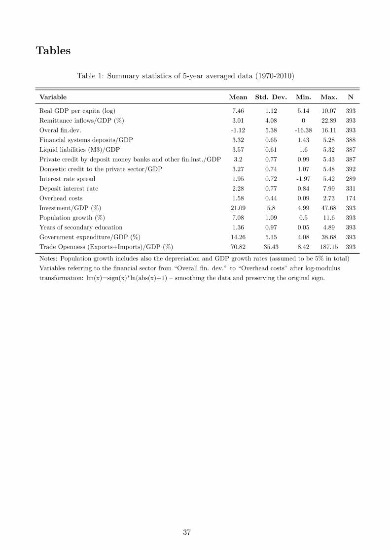
Tables

Table 1: Summary statistics of 5-year averaged data (1970-2010)

Variable Mean Std. Dev. Min. Max. N

Real GDP per capita (log) 7.46 1.12 5.14 10.07 393

Remittance inflows/GDP (%) 3.01 4.08 0 22.89 393

Overal fin.dev. -1.12 5.38 -16.38 16.11 393

Financial systems deposits/GDP 3.32 0.65 1.43 5.28 388

Liquid liabilities (M3)/GDP 3.57 0.61 1.6 5.32 387

Private credit by deposit money banks and other fin.inst./GDP 3.2 0.77 0.99 5.43 387

Domestic credit to the private sector/GDP 3.27 0.74 1.07 5.48 392

Interest rate spread 1.95 0.72 -1.97 5.42 289

Deposit interest rate 2.28 0.77 0.84 7.99 331

Overhead costs 1.58 0.44 0.09 2.73 174

Investment/GDP (%) 21.09 5.8 4.99 47.68 393

Population growth (%) 7.08 1.09 0.5 11.6 393

Years of secondary education 1.36 0.97 0.05 4.89 393

Government expenditure/GDP (%) 14.26 5.15 4.08 38.68 393

Trade Openness (Exports+Imports)/GDP (%) 70.82 35.43 8.42 187.15 393

Notes: Population growth includes also the depreciation and GDP growth rates (assumed to be 5% in total)

Variables referring to the financial sector from “Overall fin. dev.” to “Overhead costs” after log-modulus

transformation: lm(x)=sign(x)*ln(abs(x)+1) – smoothing the data and preserving the original sign.

37

Table 2: Main QML-FE results (1970-2010)

(1) (2) (3) (4)

Overall fin.cond. Financial systems deposits/GDP Priv. credit/GDP Interest rate spread

b/se b/se b/se b/se

L.Real GDP per capita (log) 0.863*** 0.860*** 0.861*** 0.814***

(0.044) (0.048) (0.046) (0.054)

Remittance inflows/GDP 0.004 0.019 0.020** -0.007

(0.003) (0.013) (0.009) (0.013)

Financial development (findev) 0.001 -0.006 -0.000 -0.011

(0.003) (0.030) (0.018) (0.026)

Remittance-findev interaction term -0.001* -0.004 -0.005** 0.004

(0.000) (0.003) (0.002) (0.006)

Investment/GDP 0.008*** 0.008*** 0.007*** 0.008***

(0.002) (0.002) (0.002) (0.002)

Population growth -0.000 0.001 0.001 0.008

(0.015) (0.017) (0.017) (0.015)

Years of secondary education 0.039 0.046* 0.043* 0.069**

(0.026) (0.026) (0.025) (0.034)

Government expenditure/GDP -0.005* -0.004 -0.004* -0.006

(0.003) (0.003) (0.003) (0.004)

Trade Openness 0.001 0.001* 0.001* 0.001**

(0.001) (0.000) (0.000) (0.001)

Observations 332 327 326 227

Countries 61 61 61 53

no. of obs. per country 5.443 5.361 5.344 4.283

Notes: The dependent variable in all columns is the natural logarithm of real GDP per capita. More explanatory notes are below Tab. 4.

Bootstrapped standard errors in parentheses, ∗ p < 0.10, ∗∗ p < 0.05, ∗∗∗ p < 0.01

All regressions include country fixed effects, time dummies (for the 5-year periods) and a constant.

Table 3: The estimated effects of remittance inflows to GDP changes on GDP per capitagrowth for different measures of financial development (QML-FE results)

effect given the following measure of financial development:

(1) (2) (3) (4)

effect at: overall fin.dev. fin. sys. deposits/GDP priv. cred. by banks and fin.inst./GDP interest rate spread

mean 0.486 0.449 0.394 0.083

p-value 0.119 0.137 0.155 0.817

median 0.523 0.479 0.387 0.066

p-value 0.101 0.124 0.162 0.855

other percentiles:

10th 0.986 0.766 0.875 -0.180

p-value 0.036 0.098 0.025 0.758

25th 0.785 0.629 0.622 -0.063

p-value 0.045 0.099 0.047 0.888

75th 0.180 0.267 0.149 0.214

p-value 0.564 0.344 0.600 0.587

95th -0.260 -0.016 -0.222 0.543

p-value 0.559 0.967 0.556 0.488

average marginal effect 0.459 0.430 0.373 0.091

p-value 0.298 0.124 0.341 0.714

Notes: * p < 0.10, ** p < 0.05, *** p < 0.01

The values in the table can be directly interpreted as semi-elasticities: for the country with overall fin. dev. at the sample mean, if

remittances share in GDP changes by 1 percentage point real GDP per capita will change by 0.486% over 5 years (significant at 12%,

all effects already multiplied by 100)

38

Table 4: Main System GMM results (1970-2010)

(1) (2) (3) (4)

Overall fin.cond. Financial systems deposits/GDP Priv. credit/GDP Interest rate spread

b/se b/se b/se b/se

L.Real GDP per capita (log) 0.927*** 0.904*** 0.936*** 0.891***

(0.039) (0.053) (0.042) (0.051)

Remittance inflows/GDP 0.001 0.035* 0.052** 0.001

(0.005) (0.018) (0.021) (0.041)

Financial development (findev) 0.006 0.015 0.020 -0.000

(0.004) (0.036) (0.022) (0.051)

Remittance-findev interaction term -0.003*** -0.010** -0.016*** -0.001

(0.001) (0.005) (0.006) (0.018)

Investment/GDP 0.008** 0.009** 0.010*** 0.012**

(0.003) (0.004) (0.004) (0.005)

Population growth -0.013 -0.012 -0.006 -0.012

(0.016) (0.015) (0.013) (0.015)

Years of secondary education 0.075** 0.077* 0.058 0.082*

(0.032) (0.045) (0.040) (0.048)

Government expenditure/GDP -0.002 0.003 0.001 0.002

(0.003) (0.005) (0.003) (0.006)

Trade Openness 0.002** 0.002 0.002 0.001

(0.001) (0.001) (0.001) (0.001)

Observations 332 332 332 258

Countries 61 61 61 57

no. of obs. per country 5.443 5.443 5.443 4.526

Number of instruments 43 43 43 43

p-value for Hansen’s test 0.379 0.394 0.625 0.655

p-value for AR(1) in residuals test 0.013 0.027 0.012 0.147

p-value for AR(2) in residuals test 0.064 0.101 0.077 0.235

p-value for AR(3) in residuals test 0.177 0.148 0.165 0.282

p-value H0 : γ = 1 (one-sided) 0.032 0.038 0.067 0.019

Notes: The dependent variable in all columns is the natural logarithm of real GDP per capita. 5-year averages of all variables.

Each column presents results using different measures of financial development (findev), (1) referring to the generated index

All coefficients except for γ and δ2 (for findev) can be interpreted as semi-elasticities: for example if the investment share in GDP

increases by 1 percentage point, GDP per capita increases by 0.8%.

Coefficients in the first row (γ in (3), for L.Real GDP per capita (log)) can be used to calculate annual speed of convergence (λ)

following Mankiw et al. (1992) and Caselli, Esquivel, and Lefort (1996). Following the calculations of the latter, λ = − ln(γ)5

.

If γ = 0.863 (QMLE-FE result), then λ ≈ 3%, All values of λ in the two tables above are between 1.3% and 4.1%, which are

reasonable numbers, slightly higher than the original Mankiw et al. (1992) results but lower than those of Caselli et al. (1996).

The interpretation of δ2 (for findev, a log-modulus transformed variable) is similar to a regular elasticity (for large values of

financial development level). In particular: δ2 ≡ ∂ln(Yit)∂lm(xit)

=∂YitYit∂xit|xit|+1

, where ln(Yit) = yit (the natural logarithm of real GDP per

capita) and xit is the level of financial development underlying the log-modulus transformed values used in the above estimations.

Standard errors in parentheses, ∗ p < 0.10, ∗∗ p < 0.05, ∗∗∗ p < 0.01, bootstrapped in column (1), robust with Windmeijer’s

correction in (2)-(4). All regressions include country fixed effects, time dummies (for the 5-year periods) and a constant.

39

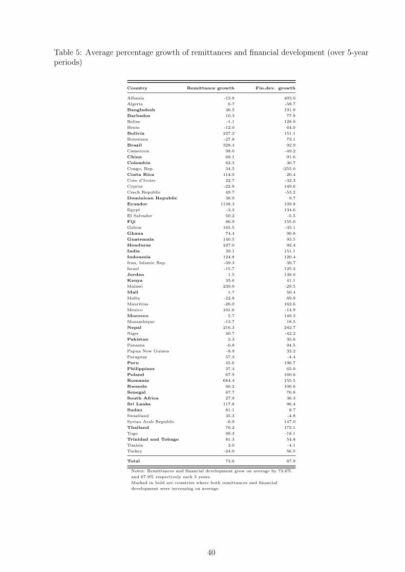
Table 5: Average percentage growth of remittances and financial development (over 5-yearperiods)

Country Remittance growth Fin.dev. growth

Albania -13.8 403.0

Algeria 6.7 -58.7

Bangladesh 36.5 191.9

Barbados 10.3 77.9

Belize -1.1 128.9

Benin -12.0 64.0

Bolivia 227.2 151.1

Botswana -27.8 73.1

Brazil 328.4 92.9

Cameroon 98.0 -49.2

China 68.1 91.6

Colombia 62.3 30.7

Congo, Rep. 34.5 -255.0

Costa Rica 114.0 20.4

Cote d’Ivoire 22.7 -32.3

Cyprus -22.8 149.6

Czech Republic 49.7 -53.2

Dominican Republic 38.9 9.7

Ecuador 1138.3 109.8

Egypt -3.2 134.6

El Salvador 50.2 -5.5

Fiji 86.9 155.0

Gabon 165.5 -35.1

Ghana 74.4 90.8

Guatemala 140.5 93.5

Honduras 227.0 92.4

India 39.1 151.1

Indonesia 124.8 120.4

Iran, Islamic Rep. -39.3 39.7

Israel -15.7 125.2

Jordan 1.5 138.0

Kenya 35.6 41.1

Malawi 239.9 -29.5

Mali 1.7 50.4

Malta -22.8 69.9

Mauritius -26.0 162.6

Mexico 101.6 -14.9

Morocco 5.7 149.3

Mozambique -13.7 18.5

Nepal 216.3 242.7

Niger 40.7 -42.2

Pakistan 2.3 35.6

Panama -0.8 94.5

Papua New Guinea -8.9 33.2

Paraguay 57.3 -4.4

Peru 45.6 196.7

Philippines 37.4 65.0

Poland 67.9 160.6

Romania 684.4 155.5

Rwanda 66.2 106.6

Senegal 67.7 76.8

South Africa 27.9 36.3

Sri Lanka 117.8 96.4

Sudan 81.1 8.7

Swaziland 35.3 -4.8

Syrian Arab Republic -6.9 147.0

Thailand 76.2 173.1

Togo 99.3 -18.1

Trinidad and Tobago 81.3 54.8

Tunisia 2.0 -4.1

Turkey -24.0 56.5

Total 73.6 67.9

Notes: Remittances and financial development grow on average by 73.6%

and 67.9% respectively each 5 years.

Marked in bold are countries where both remittances and financial

development were increasing on average.

40

Table 6: Long-run effects

Financial development at Swiss level

Overall fin.cond. Overall fin.cond. Overall fin.cond. Fin.syst.deposits/GDP Priv.credit/GDP Int.rate spread

(QML-FE) (mixed) (system GMM) (QML-FE) (QML-FE) (QML-FE)

LR effect -6.90 -15.65 -45.24 -2.14 -4.22 -1.88

std.error 4.99 8.19 377.98 3.40 3.76 3.88

p-value 0.17 0.06 0.90 0.53 0.26 0.63

Financial development at South African level

LR effect -3.78 -9.87 -29.62 0.39 -3.20 -1.57

std.error 3.27 5.11 225.56 2.10 3.27 2.69

p-value 0.25 0.05 0.90 0.85 0.33 0.56

Notes: long-run effects given different steady-state values of financial development measures (first Swiss 1990-2010 average,

then the same for South Africa).

Mixed refers to long-run effects measured with γ obtained from QML-FE estimation and δ1, δ3 from system GMM regression.

Bootstrapped standard errors.

Table 7: Coefficient estimates for the whole sample and for the sample limited to 2006

QML-FE results

Coefficient: Remittance inflows/GDP Financial development Remittance-finance interaction term Average marginal effect

Measure of financial development used: whole sample before fin.crisis whole sample before fin.crisis whole sample before fin.crisis whole sample before fin.crisis

Overall financial development 0.004 0.004 0.001 0.001 -0.001* -0.001* 0.459 0.467

s.e. (0.003) (0.003) (0.003) (0.003) (0.000) (0.000) (0.441) (0.442)

Financial system deposits to GDP ratio 0.019 0.019 -0.006 -0.003 -0.004 -0.004 0.43 0.431

s.e. (0.013) (0.012) (0.030) (0.029) (0.003) (0.003) (0.279) (0.290)

Private credit by fin. inst. to GDP ratio 0.020** 0.021** -0.000 0.001 -0.005** -0.005** 0.373 0.385

s.e. (0.009) (0.010) (0.018) (0.018) (0.002) (0.003) (0.393) (0.407)

Interest rate spread -0.007 -0.008 -0.011 -0.015 0.004 0.004 0.091 0.053

s.e. (0.013) (0.012) (0.026) (0.022) (0.006) (0.005) (0.247) (0.285)

System GMM results

Coefficient: Remittance inflows/GDP Financial development Remittance-finance interaction term Average marginal effect

Measure of financial development used: whole sample before fin.crisis whole sample before fin.crisis whole sample before fin.crisis whole sample before fin.crisis

Overall financial development 0.001 -0.000 0.006 0.003 -0.003*** -0.002*** 0.333 0.169

s.e. (0.005) (0.004) (0.004) (0.003) (0.001) (0.001) (1.443) (1.136)

Financial system deposits to GDP ratio 0.035** 0.007 0.015 -0.027 -0.010** -0.003 0.073 -0.161

s.e. (0.018) (0.016) (0.036) (0.034) (0.005) (0.004) (0.68) (0.173)

Private credit by fin. inst. to GDP ratio 0.052** 0.037 0.020 0.007 -0.016*** -0.012* -0.026 -0.16

s.e. (0.021) (0.023) (0.022) (0.026) (0.006) (0.006) (1.274) (0.942)

Interest rate spread 0.001 0.017 -0.000 - 0.003 -0.001 -0.009 -0.084 -0.002

s.e. (0.041) (0.030) (0.051) (0.030) (0.018) (0.013) (0.059) (0.571)

Notes: The values in the table can be interpreted as semi-elasticities (need to be multiplied by 100): the average marginal effect of remittances given financial development values observed in

the sample is 0.005, hence if the remittances share in GDP changes by 1 percentage point real GDP per capita will change by 0.5% = 0.005 ∗ 100% over 5 years (not statistically significant).

* p < 0.10, ** p < 0.05, *** p < 0.01

41

Figures

Figure 1: Foreign flows to developing countries – remittances larger than official develop-ment assistance (ODA) and more stable than foreign direct investment flows (FDI)

02

00

40

06

00

80

0

1990 1995 2000 2005 2010 2015year

FDI ODA

Remittances Pvt.debt&port.equity

Source: World Bank Migration and Development Brief from April 13, 2015

42

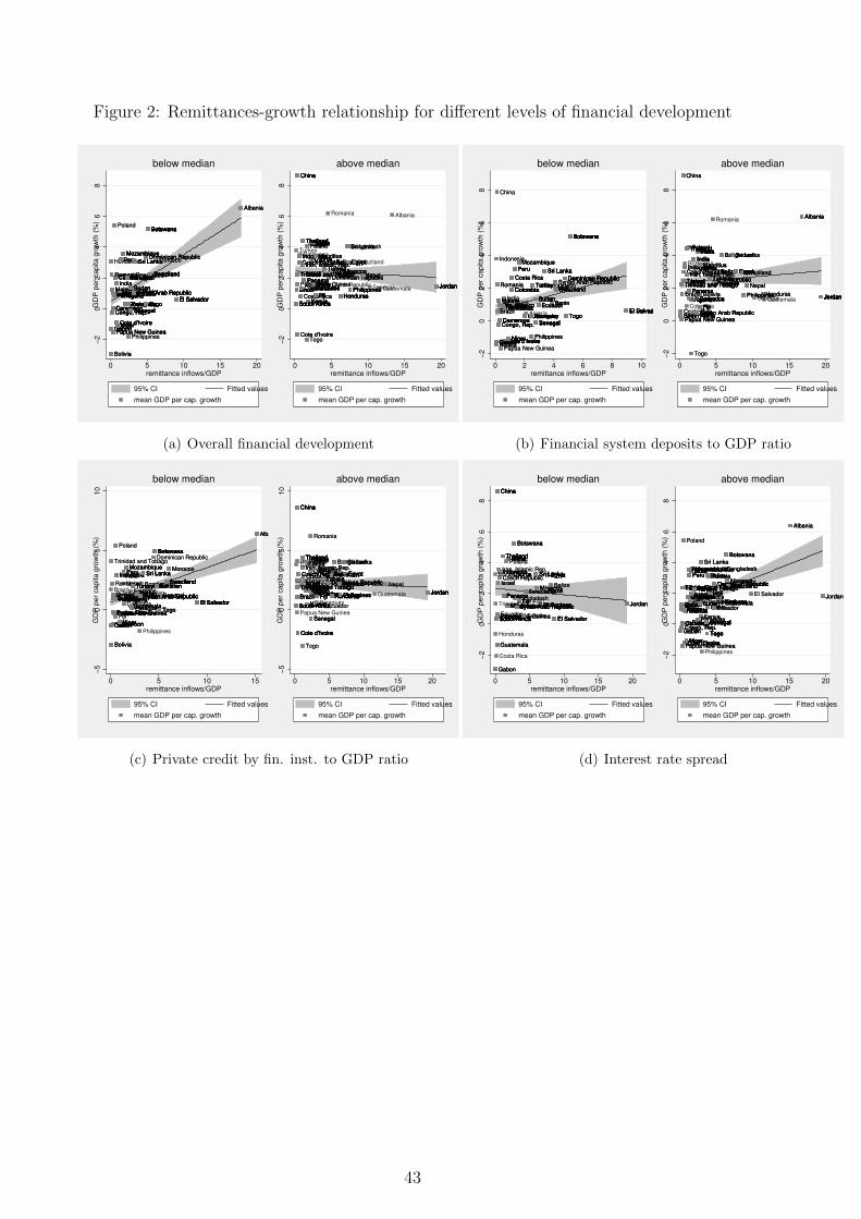
Figure 2: Remittances-growth relationship for different levels of financial development

AlbaniaAlbaniaAlbania

AlgeriaAlgeriaAlgeriaAlgeria

BangladeshBangladeshBangladesh

BeninBeninBeninBenin

BoliviaBoliviaBolivia

BotswanaBotswanaBotswanaBotswanaBotswanaBotswanaBotswana

CameroonCameroonCameroonCameroonCameroonCameroonCameroon

ColombiaColombiaColombiaColombiaColombia

Congo, Rep.Congo, Rep.Congo, Rep.Congo, Rep.Congo, Rep.

Costa RicaCosta RicaCosta RicaCosta Rica

Cote d’IvoireCote d’IvoireCote d’IvoireCote d’IvoireCote d’Ivoire

Dominican RepublicDominican RepublicDominican RepublicDominican Republic

EcuadorEcuadorEcuadorEcuadorEcuadorEl SalvadorEl SalvadorEl SalvadorEl SalvadorEl SalvadorEl SalvadorEl Salvador

GabonGabonGabonGabonGabonGabonGabon

GhanaGhanaGhanaGhanaGhanaGhanaGhana

GuatemalaGuatemalaGuatemalaGuatemalaGuatemalaGuatemala

HondurasHonduras

IndiaIndiaIndiaMalawiMalawiMalawiMalawi

MaliMaliMaliMaliMali

MexicoMexicoMexicoMexicoMexicoMexicoMexico

MoroccoMoroccoMozambiqueMozambiqueMozambiqueMozambiqueMozambique

NigerNigerNigerNigerNigerNigerPapua New GuineaPapua New GuineaPapua New GuineaPapua New Guinea

ParaguayParaguayParaguayParaguay

PeruPeruPeruPeru

PhilippinesPhilippines

PolandPoland

RomaniaRomaniaRomania

RwandaRwandaRwandaRwandaRwandaRwandaRwanda

SenegalSenegalSenegalSenegalSenegalSenegalSenegal

Sri LankaSri LankaSri LankaSri LankaSri Lanka

SudanSudanSudanSudanSudanSudanSudan

SwazilandSwazilandSwazilandSwazilandSwazilandSwazilandSwaziland

Syrian Arab RepublicSyrian Arab RepublicSyrian Arab RepublicSyrian Arab RepublicSyrian Arab RepublicSyrian Arab Republic

TogoTogoTogoTogo

TurkeyTurkeyTurkeyTurkeyTurkeyTurkeyTurkey

−2

02

46

8G

DP

pe

r ca

pita

gro

wth

(%

)

0 5 10 15 20remittance inflows/GDP

95% CI Fitted values

mean GDP per cap. growth

below median

Albania

AlgeriaAlgeriaAlgeriaAlgeria

BangladeshBangladesh

BarbadosBarbadosBarbadosBarbadosBarbadosBarbadosBarbadosBarbados

BelizeBelizeBelizeBelizeBelizeBelize

BoliviaBoliviaBoliviaBolivia

Botswana

BrazilBrazilBrazilBrazilBrazilBrazil

ChinaChinaChinaChinaChina

ColombiaColombiaColombia

Costa RicaCosta RicaCosta Rica

Cote d’IvoireCote d’IvoireCote d’Ivoire

CyprusCyprusCyprusCyprusCyprusCyprusCyprusCzech RepublicCzech RepublicCzech RepublicCzech Republic

Dominican RepublicDominican RepublicDominican RepublicDominican Republic

EgyptEgyptEgyptEgyptEgyptEgypt

FijiFijiFijiFijiFijiFiji

Guatemala

HondurasHondurasHondurasHondurasHondurasHonduras

IndiaIndiaIndiaIndiaIndia

IndonesiaIndonesiaIndonesiaIndonesiaIndonesia

Iran, Islamic Rep.Iran, Islamic Rep.Iran, Islamic Rep.Iran, Islamic Rep.

IsraelIsraelIsraelIsraelIsraelIsraelIsraelIsrael

JordanJordanJordanJordanJordanJordanJordan

KenyaKenyaKenyaKenyaKenyaKenyaKenya

MaltaMaltaMaltaMaltaMaltaMaltaMaltaMalta

MauritiusMauritiusMauritiusMauritius

MoroccoMoroccoMoroccoMoroccoMoroccoMoroccoNepalNepalNepalPakistanPakistanPakistanPakistanPakistanPakistan

PanamaPanamaPanamaPanamaPanamaPanamaPapua New GuineaPapua New Guinea

PhilippinesPhilippinesPhilippinesPhilippinesPhilippines

PolandPoland

Romania

Senegal

South AfricaSouth AfricaSouth AfricaSouth AfricaSouth AfricaSouth AfricaSouth AfricaSouth Africa

Sri LankaSri LankaSri Lanka

Swaziland

Syrian Arab Republic

ThailandThailandThailandThailandThailandThailandThailand

TogoTogo

Trinidad and TobagoTrinidad and TobagoTrinidad and TobagoTrinidad and TobagoTrinidad and TobagoTrinidad and TobagoTrinidad and TobagoTunisiaTunisiaTunisiaTunisiaTunisiaTunisia

Turkey

−2

02

46

8G

DP

pe

r ca

pita

gro

wth

(%

)

0 5 10 15 20remittance inflows/GDP

95% CI Fitted values

mean GDP per cap. growth

above median

(a) Overall financial development

Algeria

BangladeshBangladesh

BeninBeninBeninBenin

BoliviaBoliviaBoliviaBolivia

BotswanaBotswanaBotswanaBotswanaBotswanaBotswanaBotswana

BrazilBrazilBrazil

CameroonCameroonCameroonCameroonCameroonCameroonCameroon

ChinaChina

ColombiaColombiaColombiaColombiaColombiaColombiaColombia

Congo, Rep.Congo, Rep.Congo, Rep.Congo, Rep.

Costa RicaCosta RicaCosta RicaCosta Rica

Cote d’IvoireCote d’IvoireCote d’IvoireCote d’IvoireCote d’IvoireCote d’IvoireCote d’IvoireCote d’Ivoire

Dominican RepublicDominican RepublicDominican RepublicDominican RepublicDominican RepublicDominican RepublicDominican RepublicDominican Republic

EcuadorEcuadorEcuadorEcuadorEcuadorEl SalvadorEl SalvadorEl SalvadorEl SalvadorEl SalvadorEl SalvadorEl Salvador

GabonGabonGabonGabonGabonGabonGabon

GhanaGhanaGhanaGhanaGhanaGhanaGhana

GuatemalaGuatemalaGuatemalaGuatemalaGuatemalaGuatemala

HondurasHondurasHondurasHondurasHonduras

IndiaIndia

IndonesiaIndonesia

IsraelMalawiMalawiMalawiMalawi

MaliMaliMaliMaliMali

MexicoMexicoMexicoMexicoMexicoMexico

MozambiqueMozambiqueMozambiqueMozambique

NigerNigerNigerNigerNigerNiger

Papua New GuineaPapua New Guinea

ParaguayParaguayParaguayParaguay

PeruPeruPeruPeru

PhilippinesPhilippinesPhilippines

RomaniaRomaniaRomania

RwandaRwandaRwandaRwandaRwandaRwandaRwanda

SenegalSenegalSenegalSenegalSenegalSenegalSenegal

Sri LankaSri LankaSri LankaSri LankaSri Lanka

SudanSudanSudanSudanSudanSudanSudan

SwazilandSwazilandSwazilandSwazilandSwaziland

Syrian Arab RepublicSyrian Arab RepublicSyrian Arab Republic

TogoTogoTogoTogo

TurkeyTurkeyTurkeyTurkeyTurkeyTurkey

−2

02

46

8G

DP

pe

r ca

pita

gro

wth

(%

)

0 2 4 6 8 10remittance inflows/GDP

95% CI Fitted values

mean GDP per cap. growth

below median

AlbaniaAlbaniaAlbaniaAlbania

AlgeriaAlgeriaAlgeriaAlgeriaAlgeriaAlgeriaAlgeria

BangladeshBangladeshBangladesh

BarbadosBarbadosBarbadosBarbadosBarbadosBarbadosBarbadosBarbados

BelizeBelizeBelizeBelizeBelizeBelize

BoliviaBoliviaBolivia

Botswana

BrazilBrazilBrazil

ChinaChinaChina

ColombiaCosta RicaCosta RicaCosta Rica

CyprusCyprusCyprusCyprusCyprusCyprusCyprusCzech RepublicCzech RepublicCzech RepublicCzech Republic EgyptEgyptEgyptEgyptEgyptEgyptEgypt

FijiFijiFijiFijiFijiFiji

GuatemalaHondurasHondurasHonduras

IndiaIndiaIndiaIndiaIndiaIndia

IndonesiaIndonesiaIndonesiaIndonesia

Iran, Islamic Rep.Iran, Islamic Rep.Iran, Islamic Rep.Iran, Islamic Rep.IsraelIsraelIsraelIsraelIsraelIsraelIsrael

JordanJordanJordanJordanJordanJordanJordan

KenyaKenyaKenyaKenyaKenyaKenyaKenya

MaltaMaltaMaltaMaltaMaltaMaltaMaltaMalta

MauritiusMauritiusMauritiusMauritius

Mexico

MoroccoMoroccoMoroccoMoroccoMoroccoMoroccoMoroccoNepalNepalNepalPakistanPakistanPakistanPakistanPakistanPakistan

PanamaPanamaPanamaPanamaPanamaPanama

Papua New GuineaPapua New GuineaPapua New GuineaPapua New Guinea

PhilippinesPhilippinesPhilippinesPhilippines

PolandPolandPoland

Romania

Senegal

South AfricaSouth AfricaSouth AfricaSouth AfricaSouth AfricaSouth AfricaSouth AfricaSouth Africa

Sri LankaSri LankaSri Lanka

SwazilandSwazilandSwaziland

Syrian Arab RepublicSyrian Arab RepublicSyrian Arab RepublicSyrian Arab Republic

ThailandThailandThailandThailandThailandThailandThailandThailand

TogoTogo

Trinidad and TobagoTrinidad and TobagoTrinidad and TobagoTrinidad and TobagoTrinidad and TobagoTrinidad and TobagoTrinidad and TobagoTrinidad and TobagoTunisiaTunisiaTunisiaTunisiaTunisiaTunisiaTurkeyTurkey

−2

02

46

8G

DP

pe

r ca

pita

gro

wth

(%

)

0 5 10 15 20remittance inflows/GDP

95% CI Fitted values

mean GDP per cap. growth

above median

(b) Financial system deposits to GDP ratio

AlbaniaAlbaniaAlbania

AlgeriaAlgeriaAlgeriaAlgeria

BangladeshBangladesh

BeninBeninBeninBenin

BoliviaBoliviaBolivia

BotswanaBotswanaBotswanaBotswanaBotswanaBotswanaBotswanaBotswana

Brazil

CameroonCameroonCameroonCameroonCameroon

ColombiaColombia

Congo, Rep.Congo, Rep.Congo, Rep.Congo, Rep.

Costa RicaCosta RicaCosta RicaCosta Rica

Cote d’IvoireCote d’IvoireCote d’Ivoire

Dominican RepublicDominican Republic

EcuadorEcuadorEcuador

El SalvadorEl SalvadorEl SalvadorEl SalvadorEl SalvadorEl SalvadorEl Salvador

FijiFiji

GabonGabonGabonGabonGabonGabonGabon

GhanaGhanaGhanaGhanaGhanaGhanaGhana

GuatemalaGuatemalaGuatemalaGuatemalaGuatemalaGuatemala

IndiaIndiaIndiaIndiaIndonesiaIndonesiaIndonesiaIndonesia

Iran, Islamic Rep.MalawiMalawiMalawiMalawi

MaliMaliMaliMaliMali

MexicoMexicoMexicoMexicoMexicoMexicoMexico

MoroccoMoroccoMoroccoMozambiqueMozambiqueMozambiqueMozambique

NepalNepal

NigerNigerNigerNigerNigerNiger

PakistanPakistanPakistanPakistanPakistan

Papua New GuineaPapua New GuineaPapua New GuineaPapua New GuineaPapua New GuineaParaguayParaguayParaguay

PeruPeruPeruPeru

Philippines

PolandPoland

RomaniaRomania

RwandaRwandaRwandaRwandaRwandaRwandaRwandaSenegalSenegalSenegalSenegal

Sri LankaSri LankaSri LankaSri LankaSri Lanka

SudanSudanSudanSudanSudanSudanSudan

SwazilandSwazilandSwazilandSwazilandSwazilandSwazilandSwazilandSwaziland

Syrian Arab RepublicSyrian Arab RepublicSyrian Arab RepublicSyrian Arab RepublicSyrian Arab RepublicSyrian Arab RepublicSyrian Arab Republic

TogoTogoTogoTogo

Trinidad and TobagoTrinidad and Tobago

TurkeyTurkeyTurkeyTurkeyTurkeyTurkeyTurkey

−5

05

10

GD

P p

er

ca

pita

gro

wth

(%

)

0 5 10 15remittance inflows/GDP

95% CI Fitted values

mean GDP per cap. growth

below median

AlgeriaAlgeriaAlgeriaAlgeria

BangladeshBangladeshBangladesh

BarbadosBarbadosBarbadosBarbadosBarbadosBarbadosBarbadosBarbados

BelizeBelizeBelizeBelizeBelizeBelize

BoliviaBoliviaBoliviaBoliviaBrazilBrazilBrazilBrazilBrazil

CameroonCameroon

ChinaChinaChinaChinaChina

ColombiaColombiaColombiaColombiaColombiaColombia

Costa RicaCosta RicaCosta Rica

Cote d’IvoireCote d’IvoireCote d’IvoireCote d’IvoireCote d’Ivoire

CyprusCyprusCyprusCyprusCyprusCyprusCyprusCzech RepublicCzech RepublicCzech RepublicCzech Republic

Dominican RepublicDominican RepublicDominican RepublicDominican RepublicDominican RepublicDominican Republic

EcuadorEcuador

EgyptEgyptEgyptEgyptEgyptEgypt

FijiFijiFijiFijiFiji GuatemalaHondurasHondurasHondurasHondurasHondurasHondurasHonduras

IndiaIndiaIndiaIndiaIndonesiaIndonesiaIran, Islamic Rep.Iran, Islamic Rep.Iran, Islamic Rep.

IsraelIsraelIsraelIsraelIsraelIsraelIsraelIsrael

JordanJordanJordanJordanJordanJordanJordan

KenyaKenyaKenyaKenyaKenyaKenyaKenya

MaltaMaltaMaltaMaltaMaltaMaltaMaltaMalta

MauritiusMauritiusMauritiusMauritius

MoroccoMoroccoMoroccoMoroccoMorocco NepalNepal

PakistanPakistan

PanamaPanamaPanamaPanamaPanamaPanama

Papua New Guinea

Paraguay

PhilippinesPhilippinesPhilippinesPhilippinesPhilippinesPhilippines

PolandPoland

RomaniaRomania

SenegalSenegalSenegalSenegal

South AfricaSouth AfricaSouth AfricaSouth AfricaSouth AfricaSouth AfricaSouth AfricaSouth Africa

Sri LankaSri LankaSri LankaThailandThailandThailandThailandThailandThailandThailand

TogoTogo

Trinidad and TobagoTrinidad and TobagoTrinidad and TobagoTrinidad and TobagoTrinidad and TobagoTrinidad and Tobago

TunisiaTunisiaTunisiaTunisiaTunisiaTunisia

Turkey

−5

05

10

GD

P p

er

ca

pita

gro

wth

(%

)

0 5 10 15 20remittance inflows/GDP

95% CI Fitted values

mean GDP per cap. growth

above median

(c) Private credit by fin. inst. to GDP ratio

AlgeriaAlgeriaAlgeria

BangladeshBangladesh

BarbadosBarbadosBarbadosBarbadosBarbados

BelizeBelize

BotswanaBotswanaBotswanaBotswana

ChinaChinaChinaChinaChina

Costa Rica

CyprusCyprusCyprusCyprusCyprusCyprusCyprusCzech RepublicCzech RepublicCzech Republic

EcuadorEcuador

EgyptEgyptEgyptEgyptEgypt

El SalvadorEl SalvadorEl SalvadorEl SalvadorEl Salvador

FijiFijiFijiFiji

GabonGabonGabon

GuatemalaGuatemalaGuatemala

Honduras

IndonesiaIndonesiaIndonesiaIndonesiaIndonesiaIran, Islamic Rep.Iran, Islamic Rep.

IsraelIsraelIsrael

JordanJordanJordanJordan

KenyaKenyaKenyaKenyaKenya

MaltaMaltaMaltaMaltaMaltaMaltaMalta

Mauritius

MexicoMexicoMexico

MoroccoMoroccoMoroccoMoroccoNepalNepalNepalNepal

PakistanPanamaPanamaPanamaPanamaPanama

Papua New GuineaPapua New GuineaPapua New Guinea

PhilippinesPhilippinesPhilippinesPhilippinesPhilippinesPhilippines

PolandPoland

South AfricaSouth AfricaSouth AfricaSouth AfricaSouth AfricaSouth AfricaSouth Africa

Sri LankaSri LankaSri LankaSri LankaSri Lanka

SwazilandSwazilandSwaziland

Syrian Arab RepublicSyrian Arab RepublicSyrian Arab RepublicSyrian Arab RepublicSyrian Arab RepublicSyrian Arab RepublicSyrian Arab Republic

ThailandThailandThailandThailandThailandThailandThailand

Trinidad and Tobago

TunisiaTunisia

−2

02

46

8G

DP

pe

r ca

pita

gro

wth

(%

)

0 5 10 15 20remittance inflows/GDP

95% CI Fitted values

mean GDP per cap. growth

below median

AlbaniaAlbaniaAlbania

AlgeriaAlgeriaAlgeriaAlgeriaAlgeria

BangladeshBangladeshBangladesh

BarbadosBarbadosBarbados

BelizeBelizeBelizeBelize

BeninBeninBeninBenin

BoliviaBoliviaBoliviaBoliviaBoliviaBoliviaBolivia

BotswanaBotswanaBotswanaBotswana

BrazilBrazilBrazilBrazilBrazilBrazil

CameroonCameroonCameroonCameroonCameroonCameroon

ColombiaColombiaColombiaColombiaColombiaColombiaColombiaColombia

Congo, Rep.Congo, Rep.Congo, Rep.Congo, Rep.

Costa RicaCosta RicaCosta RicaCosta RicaCosta RicaCosta Rica

Cote d’IvoireCote d’IvoireCote d’IvoireCote d’IvoireCote d’IvoireCote d’IvoireCote d’IvoireCote d’Ivoire

Dominican RepublicDominican RepublicDominican RepublicDominican RepublicDominican RepublicDominican RepublicDominican RepublicDominican Republic

EcuadorEcuadorEcuador

EgyptEgypt

El SalvadorEl Salvador

FijiFijiFijiGabonGabonGabonGabon

GhanaGhanaGhanaGhanaGhanaGhanaGhanaGuatemalaGuatemalaGuatemalaGuatemalaHondurasHondurasHondurasHondurasHondurasHondurasHonduras

IndiaIndiaIndiaIndiaIndiaIndiaIndiaIndia

Iran, Islamic Rep.Iran, Islamic Rep.

IsraelIsraelIsraelIsraelIsrael JordanJordanJordan

KenyaKenyaKenya

MalawiMalawiMalawiMalawi

MaliMaliMaliMaliMali

MauritiusMauritiusMauritius

MexicoMexicoMexicoMexico

MoroccoMoroccoMoroccoMorocco

MozambiqueMozambiqueMozambiqueMozambiqueMozambique

NigerNigerNigerNigerNigerNiger

PakistanPakistanPakistanPakistanPakistanPakistan

Papua New GuineaPapua New GuineaPapua New Guinea

ParaguayParaguayParaguayParaguay

PeruPeruPeruPeru

Philippines

PolandPoland

RomaniaRomaniaRomaniaRomania

RwandaRwandaRwandaRwandaRwandaRwandaRwanda

SenegalSenegalSenegalSenegalSenegalSenegalSenegalSenegal

Sri LankaSri LankaSri Lanka

SudanSudanSudanSudanSudanSudanSudan

SwazilandSwazilandSwazilandSwazilandSwaziland

TogoTogoTogoTogoTogoTogo

Trinidad and TobagoTrinidad and TobagoTrinidad and TobagoTrinidad and TobagoTrinidad and TobagoTrinidad and TobagoTrinidad and Tobago

TunisiaTunisiaTunisiaTunisia

TurkeyTurkeyTurkeyTurkeyTurkeyTurkeyTurkeyTurkey

−2

02

46

8G

DP

pe

r ca

pita

gro

wth

(%

)

0 5 10 15 20remittance inflows/GDP

95% CI Fitted values

mean GDP per cap. growth

above median

(d) Interest rate spread

43

Figure 3: Marginal effects of remittances on economic growth for different levels of financialdevelopment - system GMM and QML-FE results

−.1

−.0

50

.05

.1M

arg

ina

l e

ffe

ct

−20 −10 0 10 20Overal fin.dev.

−.1

−.0

50

.05

.1M

arg

ina

l e

ffe

ct

1 2 3 4 5Financial systems deposits/GDP

−.1

−.0

50

.05

.1M

arg

ina

l e

ffe

ct

1 2 3 4 5Private credit by deposit money banks and other fin.inst./GDP

−.1

−.0

50

.05

.1M

arg

ina

l e

ffe

ct

−1 0 1 2 3 4Interest rate spread

confidence bound (90%) marginal effect

(a) QML-FE

−.1

−.0

50

.05

.1M

arg

ina

l e

ffe

ct

−20 −10 0 10 20Overal fin.dev.

−.1

−.0

50

.05

.1M

arg

ina

l e

ffe

ct

1 2 3 4 5Financial systems deposits/GDP

−.1

−.0

50

.05

.1M

arg

ina

l e

ffe

ct

1 2 3 4 5Private credit by deposit money banks and other fin.inst./GDP

−.1

−.0

50

.05

.1M

arg

ina

l e

ffe

ct

−2 0 2 4 6

confidence bound (90%) marginal effect

(b) system GMM

44

Figure 4: Financial development in some countries with more and and less estimationprecision.

−2

0−

10

01

02

0In

de

x v

alu

e,

log

−m

od

ulu

s s

ca

le

1970 1980 1990 2000 2010year

Cyprus

−2

0−

10

01

02

0In

de

x v

alu

e,

log

−m

od

ulu

s s

ca

le

1970 1980 1990 2000 2010year

Ghana

−2

0−

10

01

02

0In

de

x v

alu

e,

log

−m

od

ulu

s s

ca

le

1970 1980 1990 2000 2010year

India

−2

0−

10

01

02

0In

de

x v

alu

e,

log

−m

od

ulu

s s

ca

le

1970 1980 1990 2000 2010year

Mexico

Confidence bound (95%) Fin.dev.index

(a) Smaller confidence bounds

−5

05

10

15

Ind

ex v

alu

e,

log

−m

od

ulu

s s

ca

le

1970 1980 1990 2000 2010year

Colombia

−5

05

10

15

Ind

ex v

alu

e,

log

−m

od

ulu

s s

ca

le

1970 1980 1990 2000 2010year

Morocco

−5

05

10

15

Ind

ex v

alu

e,

log

−m

od

ulu

s s

ca

le

1970 1980 1990 2000 2010year

Pakistan

−5

05

10

15

Ind

ex v

alu

e,

log

−m

od

ulu

s s

ca

le

1970 1980 1990 2000 2010year

South Africa

Confidence bound (95%) Fin.dev.index

(b) Larger confidence bounds

45

Figure 5: Total changes of remittance inflows to GDP ratio and financial development foreach country

Congo, Rep.

Algeria

CameroonCote d’IvoireNiger

GabonCzech Republic

Togo

Mexico

Malawi

Swaziland

El Salvador

TunisiaParaguaySudan

Dominican Republic

MozambiqueIran, Islamic Rep.

Costa Rica

Papua New Guinea

Benin

Mali

Pakistan

Colombia

South AfricaKenya

ChinaTrinidad and Tobago

Philippines

Turkey

Ecuador

Brazil

Romania

Panama

Poland

Mauritius

Malta

Botswana

Senegal

GhanaBarbados

Guatemala

PeruIndonesiaRwanda

Belize

Honduras

Sri Lanka

Nepal

Bangladesh

Egypt

JordanIsrael

Syrian Arab Republic

Cyprus

BoliviaFiji

MoroccoIndia

Albania

Thailand

−10

010

20

Tota

l re

mitta

nces c

hange (

% p

oin

ts)

−10 −5 0 5 10Total fin.dev. change (log−mod. difference)

The total changes for each country are computed as differences of remittance inflows to GDP ratio and

financial development.

46

Figure 6: Difference in total growth of GDP per capita if remittances or fin. dev. wereheld constant at their initial level.

RwandaGhanaPeru

Sudan

Bolivia

Senegal

Ecuador

India

Sri Lanka

Mali

Indonesia

Guatemala

BangladeshRomania

Nepal

Dominican Republic

Colombia

Morocco

FijiPoland

Honduras

Kenya

Trinidad and Tobago

Thailand

Philippines

Brazil

Costa Rica

BarbadosChina South Africa

−1

5−

10

−5

05

Gro

wth

ra

te d

iffe

ren

tia

l (p

erc

en

tag

e p

oin

ts)

−15 −10 −5 0 5Initial level of financial develoment (log−mod.)

Ecuador

Brazil

GhanaIndonesia

RomaniaBoliviaCosta Rica

South Africa

Honduras

ChinaTrinidad and Tobago

Thailand

Rwanda

Sri Lanka

Colombia

Guatemala

FijiIndia

Senegal

Kenya

Poland

Peru

SudanDominican Republic

Nepal

Philippines

Barbados

Bangladesh

MaliMorocco

−1

5−

10

−5

05

Gro

wth

ra

te d

iffe

ren

tia

l (p

erc

en

tag

e p

oin

ts)

0 2 4 6Initial level of remittances to GDP ratio

90% CI Fitted values

Growth rate differential with no remit. growth

(a) No remittance change

Ecuador

BrazilGhanaIndonesia

Romania

Bolivia

Costa RicaSouth Africa

Honduras

ChinaTrinidad and Tobago

Thailand

Rwanda

Sri Lanka

Colombia

GuatemalaFiji

India

Senegal

Kenya

PolandPeru

Sudan

Dominican Republic

Nepal

Philippines

Barbados

Bangladesh

Mali

Morocco

−5

05

10

15

Gro

wth

ra

te d

iffe

ren

tia

l (p

erc

en

tag

e p

oin

ts)

0 2 4 6Initial level of remittances to GDP ratio

RwandaGhana

Peru

Sudan

Bolivia

Senegal

EcuadorIndia

Sri Lanka

MaliIndonesia

Guatemala

Bangladesh

Romania

Nepal

Dominican Republic

Colombia

Morocco

Fiji

Poland

Honduras

Kenya

Trinidad and Tobago

Thailand

Philippines

BrazilCosta Rica

Barbados

China South Africa

−5

05

10

15

Gro

wth

ra

te d

iffe

ren

tia

l (p

erc

en

tag

e p

oin

ts)

−15 −10 −5 0 5Initial level of financial development (log−mod.)

90% CI Fitted values

Growth rate differential with no fin.dev.growth

(b) No fin. dev. change

Note: The graphs show the difference between the counterfactual and real total growth of GDP per capita

(in percentage points). Positive numbers indicate output gains from the counterfactual scenario.

47

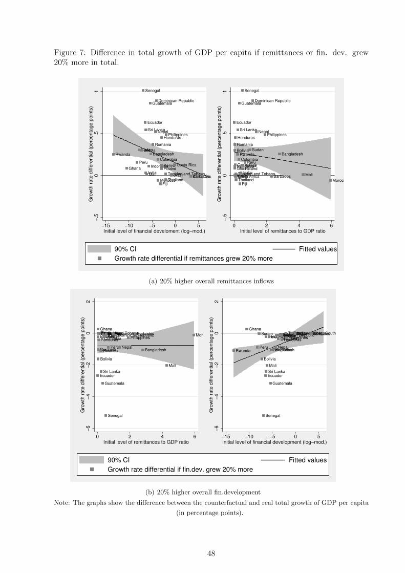
Figure 7: Difference in total growth of GDP per capita if remittances or fin. dev. grew20% more in total.

Rwanda

Ghana

Peru

SudanBolivia

Senegal

Ecuador

India

Sri Lanka

Mali

Indonesia

Guatemala

Bangladesh

Romania

Nepal

Dominican Republic

Colombia

MoroccoFiji

Poland

Honduras

Kenya

Trinidad and Tobago

Thailand

Philippines

Brazil

Costa Rica

BarbadosChina South Africa

−.5

0.5

1G

row

th r

ate

diffe

ren

tia

l (p

erc

en

tag

e p

oin

ts)

−15 −10 −5 0 5Initial level of financial develoment (log−mod.)

Ecuador

Brazil

GhanaIndonesia

Romania

Bolivia

Costa Rica

South Africa

Honduras

ChinaTrinidad and Tobago

Thailand

Rwanda

Sri Lanka

Colombia

Guatemala

Fiji

India

Senegal

KenyaPoland

Peru

Sudan

Dominican Republic

NepalPhilippines

Barbados

Bangladesh

Mali

Morocco

−.5

0.5

1G

row

th r

ate

diffe

ren

tia

l (p

erc

en

tag

e p

oin

ts)

0 2 4 6Initial level of remittances to GDP ratio

90% CI Fitted values

Growth rate differential if remittances grew 20% more

(a) 20% higher overall remittances inflows

Ecuador

BrazilGhana

Indonesia

Romania

Bolivia

Costa RicaSouth Africa

Honduras

ChinaTrinidad and TobagoThailand

Rwanda

Sri Lanka

Colombia

Guatemala

FijiIndia

Senegal

KenyaPoland

Peru

SudanDominican Republic

Nepal

PhilippinesBarbados

Bangladesh

Mali

Morocco

−6

−4

−2

02

Gro

wth

ra

te d

iffe

ren

tia

l (p

erc

en

tag

e p

oin

ts)

0 2 4 6Initial level of remittances to GDP ratio

Rwanda

Ghana

Peru

Sudan

Bolivia

Senegal

Ecuador

India

Sri Lanka

Mali

Indonesia

Guatemala

BangladeshRomaniaNepal

Dominican RepublicColombiaMoroccoFijiPoland

HondurasKenya

Trinidad and TobagoThailandPhilippines

BrazilCosta RicaBarbadosChina South Africa

−6

−4

−2

02

Gro

wth

ra

te d

iffe

ren

tia

l (p

erc

en

tag

e p

oin

ts)

−15 −10 −5 0 5Initial level of financial development (log−mod.)

90% CI Fitted values

Growth rate differential if fin.dev. grew 20% more

(b) 20% higher overall fin.development

Note: The graphs show the difference between the counterfactual and real total growth of GDP per capita

(in percentage points).

48

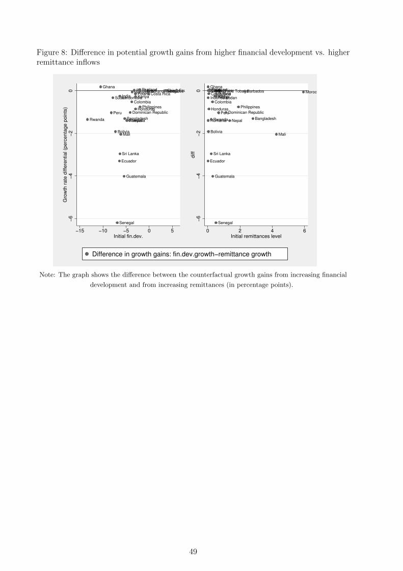
Figure 8: Difference in potential growth gains from higher financial development vs. higherremittance inflows

Rwanda

Ghana

Peru

Sudan

Bolivia

Senegal

Ecuador

India

Sri Lanka

Mali

Indonesia

Guatemala

BangladeshRomaniaNepal

Dominican Republic

Colombia

MoroccoFijiPoland

Honduras

Kenya

Trinidad and TobagoThailand

Philippines

BrazilCosta Rica

BarbadosChina South Africa

−6

−4

−2

0G

row

th r

ate

diffe

ren

tia

l (p

erc

en

tag

e p

oin

ts)

−15 −10 −5 0 5Initial fin.dev.

Ecuador

BrazilGhana

Indonesia

Romania

Bolivia

Costa RicaSouth Africa

Honduras

ChinaTrinidad and TobagoThailand

Rwanda

Sri Lanka

Colombia

Guatemala

Fiji

India

Senegal

KenyaPoland

Peru

Sudan

Dominican Republic

Nepal

Philippines

Barbados

Bangladesh

Mali

Morocco

−6

−4

−2

0d

iff

0 2 4 6Initial remittances level

Difference in growth gains: fin.dev.growth−remittance growth

Note: The graph shows the difference between the counterfactual growth gains from increasing financial

development and from increasing remittances (in percentage points).

49

Figure 9: Marginal effects of remittances on economic growth for different levels of financialdevelopment – before the financial crisis – system GMM and QML-FE results

−.1

−.0

50

.05

.1M

arg

ina

l e

ffe

ct

−20 −10 0 10 20Overal fin.dev.

−.1

−.0

50

.05

.1M

arg

ina

l e

ffe

ct

1 2 3 4 5Financial systems deposits/GDP

−.1

−.0

50

.05

.1M

arg

ina

l e

ffe

ct

1 2 3 4 5Private credit by deposit money banks and other fin.inst./GDP

−.1

−.0

50

.05

.1M

arg

ina

l e

ffe

ct

−1 0 1 2 3 4Interest rate spread

confidence bound (90%) marginal effect

(a) QML-FE

−.1

−.0

50

.05

.1M

arg

ina

l e

ffe

ct

−20 −10 0 10 20Overal fin.dev.

−.1

−.0

50

.05

.1M

arg

ina

l e

ffe

ct

1 2 3 4 5Financial systems deposits/GDP

−.1

−.0

50

.05

.1M

arg

ina

l e

ffe

ct

1 2 3 4 5Private credit by deposit money banks and other fin.inst./GDP

−.1

−.0

50

.05

.1M

arg

ina

l e

ffe

ct

−2 0 2 4 6Interest rate spread

confidence bound (90%) marginal effect

(b) system GMM

50

A Appendices

A.1 Estimation sample - country list

Country No. N From To

Albania 1 4 1995 2010

Algeria 2 8 1975 2010

Bangladesh 3 5 1990 2010

Barbados 4 8 1975 2010

Belize 5 6 1985 2010

Benin 6 4 1995 2010

Bolivia 7 7 1980 2010

Botswana 8 8 1975 2010

Brazil 9 6 1985 2010

Cameroon 10 7 1980 2010

China 11 5 1990 2010

Colombia 12 8 1975 2010

Congo, Rep. 13 5 1990 2010

Costa Rica 14 7 1980 2010

Cote d’Ivoire 15 8 1975 2010

Cyprus 16 7 1980 2010

Czech Republic 17 4 1995 2010

Dominican Republ 18 8 1975 2010

Ecuador 19 5 1990 2010

Egypt 20 7 1980 2010

El Salvador 21 7 1980 2010

Fiji 22 7 1980 2010

Gabon 23 7 1980 2010

Ghana 24 7 1980 2010

Guatemala 25 7 1980 2010

Honduras 26 8 1975 2010

India 27 8 1975 2010

Indonesia 28 6 1985 2010

Iran, Islamic Re 29 4 1995 2010

Israel 30 8 1975 2010

Jordan 31 7 1980 2010

Kenya 32 8 1975 2010

Malawi 33 4 1995 2010

Mali 34 5 1990 2010

Malta 35 8 1975 2010

Mauritius 36 4 1995 2010

Mexico 37 7 1980 2010

Morocco 38 8 1975 2010

Mozambique 39 5 1990 2010

Nepal 40 4 1995 2010

Niger 41 6 1985 2010

Pakistan 42 7 1980 2010

Panama 43 6 1985 2010

Papua New Guinea 44 6 1980 2005

Paraguay 45 4 1995 2010

Peru 46 4 1995 2010

Philippines 47 7 1980 2010

Poland 48 4 1995 2010

Romania 49 4 1995 2010

Rwanda 50 7 1980 2010

Senegal 51 8 1975 2010

South Africa 52 8 1975 2010

Sri Lanka 53 8 1975 2010

Sudan 54 7 1980 2010

Swaziland 55 8 1975 2010

Syrian Arab Repu 56 7 1980 2010

Thailand 57 8 1975 2010

Togo 58 6 1985 2010

Trinidad and Tob 59 8 1975 2010

Tunisia 60 6 1985 2010

Turkey 61 8 1975 2010

Total 393 Av. per country 6.44

51

A.2 Kalman filter and MLE

The overall financial development index has been obtained by applying the Kalman

filter to panel data. The procedure can be summarized as follows (with the country index

i dropped for simplicity). The estimation has been done in Stata/Mata.

1. Initialization: s0|0 = 0 (for a stationary process) or other arbitrary or estimated

initialization (from a normal distribution) for a nonstationary process, P0|0 = 11−γ2 ,

initial guess for θ = (α,β, vech(Σ))

2. Kalman forecasting and updating

• st+1|t = γst|t (forecasted financial development index)

• Pt+1|t = γ2 + 1 (variance of the index forecast)

• ηt = zt+1 − zt+1|t = zt+1 − α− βιst+1|t = βι(st+1 − st+1|t) + wt+1

• Ft ≡ E(ηtηt′) = βιPt+1|tι

′β′ + Σ

• st+1|t+1 = st+1|t+Pt+1|tι′β′Ft−1ηt (updated financial development index forecast)

• Pt+1|t+1 = Pt+1|t − Pt+1|tι′β′Ft−1ιβPt+1|t (updated index forecast variance)

3. Maximum likelihood estimation:

maxθ∑T

t=1 l(Zt|It−1) =∑T

t=1[−12(log(2π) + log |Ft| + η′tFt

−1ηt)]

⇔ minθ∑T

t=1[log |Ft|+ η′tF−1t ηt]

4. State smoothing:

st|T = st|t + Jt(st+1|T − st+1|t)

Pt|T = Pt|t + Jt(Pt+1|T − Pt+1|t)Jt′

where Jt = Pt|tγP−1t+1|t

The last step of the procedure – state smoothing – is of high importance as it should help

eliminate potential jumps related to some variable becoming available later than others and

included only is some years when estimating the financial development index. To under-

stand this, let us consider the following hypothetical example. If a country had relatively

moderate values of deposits to GDP and credit to GDP ratios from 1970, but the interest

rate spread (or other measure of financial sector efficiency described in Section 3.2) becomes

available only in 1990 and reflects high inefficiency, Kalman forecasting and updating will

estimate a jump in the financial development index value in 1990. Starting at time T and

smoothing the the updated forecasts of st|t should flatten this jump.

Tab. 8 gives some empirical examples for the relevance of the backward smoothing.

Columns (1) - (3) include the values of the variables from the 3 categories considered for

the generation of index of overall financial conditions. The value of the index labeled

52

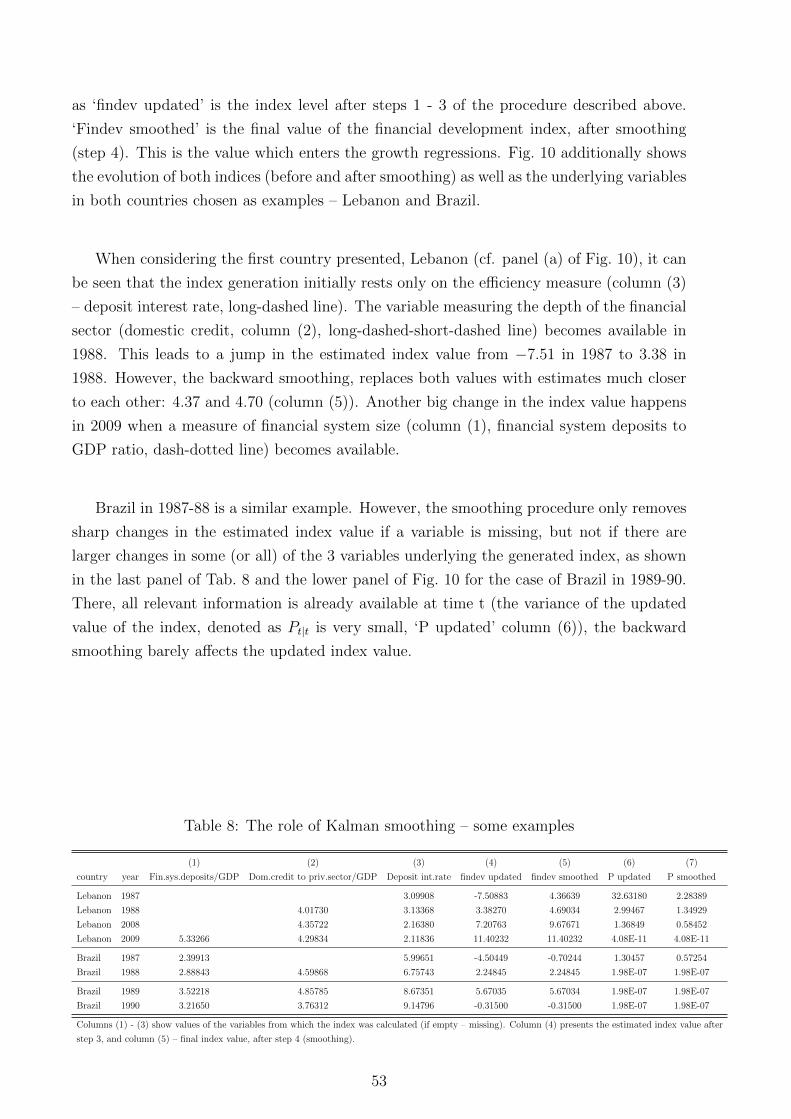
as ‘findev updated’ is the index level after steps 1 - 3 of the procedure described above.

‘Findev smoothed’ is the final value of the financial development index, after smoothing

(step 4). This is the value which enters the growth regressions. Fig. 10 additionally shows

the evolution of both indices (before and after smoothing) as well as the underlying variables

in both countries chosen as examples – Lebanon and Brazil.

When considering the first country presented, Lebanon (cf. panel (a) of Fig. 10), it can

be seen that the index generation initially rests only on the efficiency measure (column (3)

– deposit interest rate, long-dashed line). The variable measuring the depth of the financial

sector (domestic credit, column (2), long-dashed-short-dashed line) becomes available in

1988. This leads to a jump in the estimated index value from −7.51 in 1987 to 3.38 in

1988. However, the backward smoothing, replaces both values with estimates much closer

to each other: 4.37 and 4.70 (column (5)). Another big change in the index value happens

in 2009 when a measure of financial system size (column (1), financial system deposits to

GDP ratio, dash-dotted line) becomes available.

Brazil in 1987-88 is a similar example. However, the smoothing procedure only removes

sharp changes in the estimated index value if a variable is missing, but not if there are

larger changes in some (or all) of the 3 variables underlying the generated index, as shown

in the last panel of Tab. 8 and the lower panel of Fig. 10 for the case of Brazil in 1989-90.

There, all relevant information is already available at time t (the variance of the updated

value of the index, denoted as Pt|t is very small, ‘P updated’ column (6)), the backward

smoothing barely affects the updated index value.

Table 8: The role of Kalman smoothing – some examples

(1) (2) (3) (4) (5) (6) (7)

country year Fin.sys.deposits/GDP Dom.credit to priv.sector/GDP Deposit int.rate findev updated findev smoothed P updated P smoothed

Lebanon 1987 3.09908 -7.50883 4.36639 32.63180 2.28389

Lebanon 1988 4.01730 3.13368 3.38270 4.69034 2.99467 1.34929

Lebanon 2008 4.35722 2.16380 7.20763 9.67671 1.36849 0.58452

Lebanon 2009 5.33266 4.29834 2.11836 11.40232 11.40232 4.08E-11 4.08E-11

Brazil 1987 2.39913 5.99651 -4.50449 -0.70244 1.30457 0.57254

Brazil 1988 2.88843 4.59868 6.75743 2.24845 2.24845 1.98E-07 1.98E-07

Brazil 1989 3.52218 4.85785 8.67351 5.67035 5.67034 1.98E-07 1.98E-07

Brazil 1990 3.21650 3.76312 9.14796 -0.31500 -0.31500 1.98E-07 1.98E-07

Columns (1) - (3) show values of the variables from which the index was calculated (if empty – missing). Column (4) presents the estimated index value after

step 3, and column (5) – final index value, after step 4 (smoothing).

53

Figure 10: The role of smoothing after using Kalman filter and MLE

−20

−10

010

20

1980 1990 2000 2010 2020year

confidence bound findev updated confidence bound findev smoothed

Findev updated Findev smoothed

Financial system deposits/GDP Deposit interest rate

Domestic credit to private sector/GDP

(a) Lebanon

−10

−5

05

10

1970 1980 1990 2000 2010year

confidence bound findev updated confidence bound findev smoothed

Findev updated Findev smoothed

Financial system deposits/GDP Deposit interest rate

Domestic credit to private sector/GDP

(b) Brazil

The different dashed lines on the legend are the variables which were used extract the financial development index for eachcountry (could differ across countries, depending on data availability). The thinner solid line denotes the generated indexof overall financial conditions before smoothing and the thicker line are after smoothing (final values of the index enteringgrowth regressions). Different time periods are considered, vertical axis corresponds to the log-modulus scale of the variables.

54

A.3 Estimated pairwise correlations for the 5-year averaged data

(1970-2010)

1 2 3 4 5 6

1 Real GDP per capita (log) 1

2 Investment/GDP 0.245∗∗∗ 1

3 Population growth -0.425∗∗∗ -0.082 1

4 Years of secondary education 0.652∗∗∗ 0.081 -0.478∗∗∗ 1

5 Government expenditure/GDP 0.326∗∗∗ 0.246∗∗∗ 0.099∗ 0.251∗∗∗ 1

6 Trade Openness 0.418∗∗∗ 0.255∗∗∗ -0.133∗∗ 0.345∗∗∗ 0.394∗∗∗ 1

7 Remittance inflows/GDP -0.077 0.139∗∗ -0.028 0.054 0.087 0.202∗∗∗

8 Overal fin.dev. 0.536∗∗∗ 0.339∗∗∗ -0.309∗∗∗ 0.469∗∗∗ 0.294∗∗∗ 0.390∗∗∗

9 Financial systems deposits/GDP 0.490∗∗∗ 0.311∗∗∗ -0.321∗∗∗ 0.514∗∗∗ 0.310∗∗∗ 0.408∗∗∗

10 Private credit by deposit money banks and other fin.inst./GDP 0.484∗∗∗ 0.316∗∗∗ -0.235∗∗∗ 0.411∗∗∗ 0.282∗∗∗ 0.333∗∗∗

11 Interest rate spread -0.035 -0.306∗∗∗ 0.006 0.088 -0.007 -0.097

7 8 9 10 11

1 Real GDP per capita (log)

2 Investment/GDP

3 Population growth

4 Years of secondary education

5 Government expenditure/GDP

6 Trade Openness

7 Remittance inflows/GDP 1

8 Overal fin.dev. 0.100∗ 1

9 Financial systems deposits/GDP 0.157∗∗ 0.915∗∗∗ 1

10 Private credit by deposit money banks and other fin.inst./GDP 0.035 0.954∗∗∗ 0.825∗∗∗ 1

11 Interest rate spread -0.105 -0.235∗∗∗ -0.225∗∗∗ -0.212∗∗∗ 1

Notes: Significance levels: ∗ 10%, ∗∗ 5%, ∗∗∗ 1%

This table presents pairwise correlation coefficients for the data used in growth regressions in this paper.

A.4 Ranking of countries by financial development

Rank Country Fin.dev. Ranks - other measures Rank Country Fin.dev. Ranks - other measures

(1) (2) (3) (1) (2) (3)

1 Hong Kong SAR, C 14.64 1 2 48 77 Seychelles -0.57 58 118 101

2 Japan 14.05 4 1 17 78 Venezuela, RB -0.70 97 111 27

3 Luxembourg 12.94 3 8 13 79 Macedonia, FYR -0.97 111 89 106

4 Switzerland 11.43 6 4 6 80 Suriname -1.00 85 106 127

5 Cyprus 10.53 8 6 20 81 Iran, Islamic Re -1.08 80 82 1

6 United States 9.45 22 5 171 82 Zimbabwe -1.10 71 112 91

7 Netherlands 8.88 18 18 16 83 Pakistan -1.13 91 97 82

8 Macao SAR, China 8.66 5 31 53 84 Samoa -1.35 93 108 107

9 Portugal 8.60 12 16 14 85 Nicaragua -1.35 79 85 125

10 Spain 8.47 17 10 29 86 Costa Rica -1.37 108 102 144

11 Malta 8.32 7 26 26 87 Colombia -1.48 120 88 121

12 Germany 8.25 13 7 76 88 Oman -1.51 87 68 21

13 Singapore 8.22 15 14 34 89 Indonesia -1.71 101 91 38

14 Canada 8.16 20 17 23 90 Maldives -2.04 36 23 99

15 Malaysia 7.97 14 20 28 91 Papua New Guinea -2.09 96 116 90

16 Austria 7.91 19 19 36 92 Mauritania -2.24 127 90 136

17 France 7.64 23 13 47 93 Sri Lanka -2.37 105 115 8

18 United Kingdom 7.34 181 3 4 94 Turkey -2.39 103 117 171

19 St. Kitts and Ne 7.00 10 40 69 95 Dominican Republ -2.55 121 77 142

20 Sweden 6.97 89 12 51 96 Bolivia -2.57 134 100 162

21 South Africa 6.96 45 15 45 97 Solomon Islands -2.75 102 101 124

22 Lebanon 6.78 2 21 80 98 Cote d’Ivoire -2.81 128 95 114

23 Thailand 6.42 32 28 31 99 Mexico -2.85 110 113 74

24 Italy 6.19 28 27 87 100 Togo -2.95 113 114 118

25 Ireland 6.13 35 30 58 101 Swaziland -3.08 107 121 77

26 St. Lucia 5.61 30 37 97 102 Senegal -3.13 137 99 115

27 Vanuatu 5.57 9 66 108 103 Albania -3.17 55 152 89

28 China 5.56 86 9 5 104 Lesotho -3.21 83 146 109

29 Jordan 5.43 16 29 44 105 Romania -3.29 115 125 146

30 Antigua and Barb 5.30 11 25 83 106 Paraguay -3.47 131 107 160

31 Grenada 5.25 25 44 94 107 Guatemala -3.59 119 122 95

32 Panama 5.24 53 36 54 108 Libya -3.88 143 150 19

33 Norway 5.23 51 24 37 109 Benin -3.88 125 140 114

55

34 Israel 4.87 40 39 133 110 Bangladesh -3.91 73 86 39

35 Finland 4.79 54 34 22 111 Ethiopia -3.92 114 124 43

36 Barbados 4.75 38 53 72 112 Botswana -3.95 109 132 46

37 Denmark 4.74 63 55 68 113 Nepal -4.18 116 138 24

38 Czech Republic 4.65 29 50 62 114 Peru -4.23 136 128 169

39 Australia 4.61 48 43 9 115 Mongolia -4.35 118 131 164

40 Bahamas, The 4.45 49 41 15 116 Ecuador -4.53 133 104 3

41 Bahrain 4.44 39 46 65 117 Mozambique -4.54 117 142 126

42 Tunisia 4.30 57 32 42 118 Mali -4.56 146 133 114

43 St. Vincent and 4.27 27 62 98 119 Ukraine -4.62 140 139 158

44 Belgium 4.20 41 59 73 120 Argentina -4.92 139 126 40

45 Aruba 4.09 44 49 85 121 Belarus -5.59 148 143 55

46 Dominica 4.04 37 61 81 122 El Salvador -5.65 176 166 30

47 Korea, Rep. 3.88 70 33 2 123 Gabon -5.71 154 141 122

48 New Zealand 3.62 56 57 7 124 Cameroon -5.85 149 130 138

49 Kuwait 3.56 34 51 10 125 Gambia, The -5.88 132 137 150

50 Chile 3.27 68 11 96 126 Saudi Arabia -5.91 155 47 171

51 Greece 3.27 47 65 67 127 Comoros -5.96 138 148 112

52 Iceland 3.23 75 42 70 128 Haiti -6.07 126 149 161

53 Mauritius 3.22 43 67 75 129 Syrian Arab Rep. -6.32 100 157 33

54 Namibia 2.43 60 48 93 130 Nigeria -6.33 145 145 59

55 Bulgaria 2.22 67 83 154 131 Malawi -6.45 135 153 153

56 Slovenia 2.11 64 64 111 132 Zambia -6.54 144 170 117

57 Belize 2.04 59 54 88 133 Madagascar -6.58 151 134 156

58 Trinidad and Tobago 2.00 66 69 105 134 Burkina Faso -6.99 159 135 115

59 Brazil 1.93 90 72 170 135 Congo, Rep. -7.32 165 172 123

60 Morocco 1.84 62 70 11 136 Liberia -7.46 142 155 145

61 Egypt 1.79 46 75 63 137 Bhutan -8.51 50 94 130

62 Cape Verde 1.77 31 103 104 138 Burundi -8.70 163 144 116

63 Fiji 1.18 77 80 49 139 Ghana -9.41 158 165 102

64 Guyana 1.01 21 45 84 140 Sudan -9.46 162 160 171

65 Hungary 0.49 74 71 35 141 Niger -9.47 168 151 115

66 Poland 0.41 81 78 64 142 Guinea-Bissau -9.58 173 180 165

67 Kenya 0.12 78 87 100 143 Lao PDR -9.68 161 164 163

68 Philippines 0.06 84 76 52 144 Tanzania -10.34 157 167 140

69 Honduras 0.04 98 73 129 145 Central African -10.44 178 162 128

70 Latvia 0.04 104 93 113 146 Rwanda -10.63 169 174 120

71 Jamaica -0.10 76 98 134 147 Equatorial Guinea -10.89 174 163 147

72 Qatar -0.12 61 74 32 148 Uganda -11.23 170 178 132

73 Uruguay -0.12 92 96 18 149 Myanmar -11.46 167 175 66

74 Algeria -0.20 69 109 50 150 Chad -11.76 179 176 135

75 India -0.28 82 92 171 151 Sierra Leone -12.95 141 161 141

76 Tonga -0.49 94 81 71

Fin.dev. refers to the mean of the financial development index over the whole period for which data for the given country was available

Ranks based on other measures: (1) Deposits/GDP, (2) Private credit/GDP, (3) Interest rate spread

56

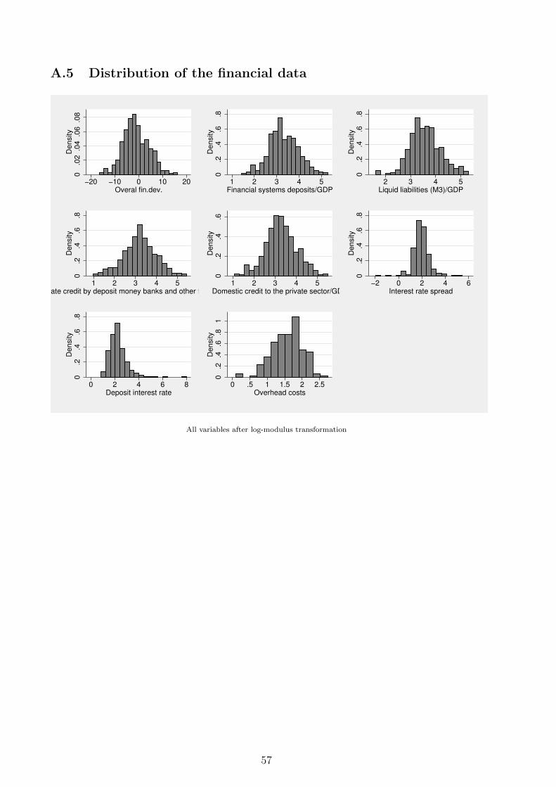
A.5 Distribution of the financial data0

.02

.04

.06

.08

De

nsity

−20 −10 0 10 20Overal fin.dev.

0.2

.4.6

.8D

en

sity

1 2 3 4 5Financial systems deposits/GDP

0.2

.4.6

.8D

en

sity

2 3 4 5Liquid liabilities (M3)/GDP

0.2

.4.6

.8D

en

sity

1 2 3 4 5Private credit by deposit money banks and other fin.inst./GDP

0.2

.4.6

De

nsity

1 2 3 4 5Domestic credit to the private sector/GDP

0.2

.4.6

.8D

en

sity

−2 0 2 4 6Interest rate spread

0.2

.4.6

.8D

en

sity

0 2 4 6 8Deposit interest rate

0.2

.4.6

.81

De

nsity

0 .5 1 1.5 2 2.5Overhead costs

All variables after log-modulus transformation

57

A.6 Marginal effects of remittances for different measures of fi-

nancial development – system GMM results

I focus on QML-FE results as main results, as they are more robust, not relying on

instrument choice. Using system GMM coefficient estimates, more appropriate if weak

exogeneity is only true for future values of the error term, but not contemporaneously,

would not change the main conclusions of positive and significant impact of remittances

on economic growth for countries with lowest financial development (but with a stronger

marginal effect) and mean and median effects would remain at similar levels.

Table 10: The estimated effects of remittance inflows to GDP changes on GDP per capitagrowth for different measures of financial development (system GMM)

effect given the following measure of financial development:

(1) (2) (3) (4)

effect at: overall fin.dev. fin. sys. deposits/GDP priv. cred. by banks and fin.inst./GDP interest rate spread

mean 0.421 0.117 0.018 -0.083

p-value 0.422 0.735 0.960 0.912

median 0.540 0.190 -0.004 -0.079

p-value 0.322 0.601 0.990 0.921

other percentiles:

10th 2.055 0.888 1.569 -0.023

p-value 0.027 0.148 0.063 0.990

25th 1.399 0.555 0.754 -0.050

p-value 0.060 0.250 0.182 0.970

75th -0.581 -0.328 -0.770 -0.113

p-value 0.202 0.285 0.009 0.848

95th -2.018 -1.017 -1.964 -0.189

p-value 0.004 0.035 0.001 0.915

average marginal effect 0.333 0.073 -0.026 -0.084

p-value 0.818 0.914 0.984 0.162

Notes: * p < 0.10, ** p < 0.05, *** p < 0.01

The values in the table can be directly interpreted as semi-elasticities: for the country with overall fin. dev. at the sample mean, if

remittances share in GDP changes by 1 percentage point real GDP per capita will change by 0.486% over 5 years (significant at 12%,

all effects already multiplied by 100)

A.7 Computation of the counterfactual scenarios - details

This analysis has only been done for 30 countries for which both remittance inflows

and financial development levels have increased between 1970-2010. Values of δ1, δ2 and δ3

are taken from the main QML-FE results.

GDP per capita in the last period can be estimated as:

yiT = α + γyi,T−1 + δ1RemiT + δ2FinDeviT + δ3RemiTFinDeviT + βXiT + ηt (10)

Iterating backward and abstracting from time effects (ηt) gives:

yiT = γTyi,0 +ΣT−1j=0 γ

j (α+δ1Remi,T−j +δ2FinDevi,T−j +δ3Remi,T−jFinDevi,T−j +βXi,T−j)

(11)

58

1. Scenario I - no remittances change or no financial development change

(a) No remittance change ⇒ Remit = Remi0∀t ∈ [0, T ]

In this case GDP per capita in the last period could be approximated by:

yiT = γTyi,0+ΣT−1j=0 γ

j (α+δ1Remi,0+δ2FinDevi,T−j+δ3Remi,0FinDevi,T−j+βXi,T−j)

(12)

and the growth rate differential (in percentage points is:):

100∗(yiT−yiT )noremitgrowth = 100∗ΣT−1j=0 γ

j(Remi0−Remi,T−j)(δ1 +δ3FinDevi,T−j)

(13)

(b) No financial development change ⇒ FinDevit = FinDevi0∀t ∈ [0, T ]

Similarly to (13):

100∗(yiT−yiT )nofindevgrowth = 100∗ΣT−1j=0 γ

j(FinDevi0−FinDevi,T−j)(δ2+δ3Remi,T−j)

(14)

2. Scenario II - Larger than observed increase of remittances or financial development

between 1970 and 2010

(a) Remittance overall growth 20% higher than observed⇒ RemiT = 1.2∗(RemiT −Remi1) + Remi1

One way to achieve the higher final level of remittances would be to affect the

whole path of remittances, such that the overall growth is 20% higher than what

was observed in reality. However, in this case some values of remittances can be

lower in the counterfactual scenario, mitigating the effect of their higher value in

the last period. For this reason, I assume that the increase of remittances took

place in the last 5-year period and previous values remained unchanged. That

means that GDP per capita is only affected by the marginal effect driven by

the difference between counterfactual and observed remittances inflows to GDP

ratio in the last period (for each country):

100 ∗ (∆yiT )remitgrowth20 = 100 ∗ (Remi,T − Remi,T )(δ1 + δ3FinDevi,T ) (15)

(b) Financial development overall growth 20% higher than observed

The assumption that the whole increase took place in the final 5-year period

for each country preserves. However, some adjustments need to be made to

transform the increase in the level of financial development into the change of

its log-modulus value.

59

Let xit denote the level of financial development. Then the counterfactual level

of financial development xiT , related to an increase 20% higher than in reality is

computed as follows:

xiT − xi0 = 1.2(xiT − xi0) (16)

the log-modulus transformed value which enters the regression equation is

defined as:

FinDevi,T = sign(xiT )(ln(|xiT |+ 1)) (17)

and the difference between the counterfactual and the real output per capita is:

100 ∗ (∆yiT )findevgrowth20 = 100 ∗ (FinDevi,T − FinDevi,T )(δ2 + δ3Remi,T ) (18)

For the sake of simplicity, I have formulated all the equations in this section

under the assumption that the panel is balanced and the final time period is the

same for each country. This is not the case in my data set, therefore in the actual

calculations T always has a subscript i, meaning that it is country specific.

By applying the Kalman filter and maximum likelihood estimation on log-

modulus transformed financial indicators, I obtained values of the unobserved

overall financial development conditions which are also on the log-modulus

scale. Therefore, to compute the counterfactual level of financial development I

first need to transform FinDevi,T into levels, according to:

xit =

{exp(FinDevi,t)− 1 if FinDevi,t ≥ 0

1− exp(−FinDevi,t) otherwise

60

A.8 Estimation results for the sample limited to 2006 (before the

financial crisis, 1970-2006)

Table 11: QML-FE results

(1) (2) (3) (4)

Overall fin.cond. Financial systems deposits/GDP Priv. credit/GDP Interest rate spread

b/se b/se b/se b/se

L.Real GDP per capita (log) 0.824*** 0.822*** 0.824*** 0.758***

(0.040) (0.045) (0.043) (0.046)

Remittance inflows/GDP 0.004 0.019 0.021** -0.008

(0.003) (0.012) (0.010) (0.012)

Financial development (findev) 0.001 -0.003 0.001 -0.015

(0.003) (0.029) (0.018) (0.022)

Remittance-findev interaction term -0.001* -0.004 -0.005* 0.004

(0.000) (0.003) (0.003) (0.005)

Investment/GDP 0.007*** 0.007*** 0.007*** 0.008***

(0.002) (0.002) (0.002) (0.003)

Population growth -0.000 0.002 0.001 0.007

(0.014) (0.015) (0.015) (0.014)

Years of secondary education 0.039* 0.044** 0.041* 0.073**

(0.022) (0.022) (0.022) (0.031)

Government expenditure/GDP -0.005 -0.004* -0.004* -0.004

(0.003) (0.003) (0.003) (0.004)

Trade Openness 0.001 0.001* 0.001* 0.001**

(0.000) (0.000) (0.000) (0.001)

Observations 331 325 324 225

Countries 61 61 61 53

average no. of obs. per country 5.443 5.361 5.344 4.283

Table 12: System GMM results

0

(1) (2) (3) (4)

Overall fin.cond. Financial systems deposits/GDP Priv. credit/GDP Interest rate spread

b/se b/se b/se b/se

L.Real GDP per capita (log) 0.940*** 0.962*** 0.959*** 0.881***

(0.036) (0.035) (0.030) (0.047)

Remittance inflows/GDP -0.000 0.007 0.037 0.017

(0.004) (0.016) (0.023) (0.030)

Financial development (findev) 0.003 -0.027 0.007 -0.003

(0.003) (0.034) (0.026) (0.030)

Remittance-findev interaction term -0.002*** -0.003 -0.012* -0.009

(0.001) (0.004) (0.006) (0.013)

Investment/GDP 0.009*** 0.010*** 0.009** 0.013***

(0.003) (0.003) (0.004) (0.003)

Population growth -0.017 -0.050* -0.024 -0.023

(0.014) (0.027) (0.020) (0.022)

Years of secondary education 0.062** 0.029 0.044* 0.086**

(0.029) (0.033) (0.025) (0.038)

Government expenditure/GDP 0.003 0.006 0.005 0.005

(0.003) (0.004) (0.004) (0.004)

Trade Openness 0.001 0.001 0.001 0.001

(0.001) (0.001) (0.001) (0.001)

Observations 331 330 330 256

Countries 61 61 61 57

average no. of obs. per country 5.443 5.443 5.443 4.526

Number of instruments 50 50 50 50

p-value for Hansen’s test 0.609 0.367 0.435 0.732

p-value for AR(1) in residuals test 0.027 0.070 0.024 0.067

p-value for AR(2) in residuals test 0.069 0.078 0.057* 0.166

p-value for AR(3) in residuals test 0.207 0.360 0.240 0.360

p-value H0 : γ = 1 (one-sided) 0.050 0.141 0.086 0.007

Notes: Bootstrapped standard errors in parentheses (in all QML-FE estimations and system GMM column (1), robust standard

errors with Windmeijer’s correction in (2)-(4) of system GMM. ∗ p < 0.10, ∗∗ p < 0.05, ∗∗∗ p < 0.01

All regressions include country fixed effects, time dummies (for the 5-year periods) and a constant.

61

A.9 Pooled OLS (POLS) and fixed effects (FE) estimation results

These results are included to show that the autoregressive coefficient in the system

GMM regressions lies in the confidence bound between within (FE) estimates and pooled

OLS results, as suggested by Roodman (2009).

Table 13: Whole sample (1970-2010)

Overall fin.cond. Financial systems deposits GDP Priv. credit GDP Interest rate spread

(1) (2) (3) (4) (5) (6) (7) (8)

(FE) (POLS) (FE) (POLS) (FE) (POLS) (FE) (POLS)

b/se b/se b/se b/se b/se b/se b/se b/se

L.Real GDP per capita (log) 0.784∗∗∗ 0.967∗∗∗ 0.780∗∗∗ 0.966∗∗∗ 0.782∗∗∗ 0.968∗∗∗ 0.716∗∗∗ 0.965∗∗∗

(0.039) (0.008) (0.039) (0.008) (0.037) (0.008) (0.048) (0.011)

Remittance inflows/GDP 0.003 0.004∗∗∗ 0.018∗∗∗ 0.024∗∗∗ 0.018∗∗∗ 0.021∗∗∗ -0.005 -0.011

(0.003) (0.001) (0.007) (0.008) (0.006) (0.005) (0.009) (0.007)

Financial development (findev) 0.001 0.005∗∗∗ 0.003 0.042∗∗∗ 0.008 0.027∗∗∗ -0.017 -0.028∗∗

(0.003) (0.001) (0.029) (0.013) (0.018) (0.010) (0.019) (0.014)

Remittance-findev interaction term -0.001∗ -0.001∗∗∗ -0.004∗∗ -0.006∗∗∗ -0.005∗∗∗ -0.006∗∗∗ 0.005 0.007∗

(0.000) (0.000) (0.002) (0.002) (0.002) (0.002) (0.005) (0.004)

Investment/GDP 0.008∗∗∗ 0.009∗∗∗ 0.008∗∗∗ 0.009∗∗∗ 0.008∗∗∗ 0.010∗∗∗ 0.008∗∗∗ 0.009∗∗∗

(0.002) (0.001) (0.002) (0.001) (0.002) (0.001) (0.003) (0.002)

Population growth -0.000 -0.020∗ 0.000 -0.021∗∗ -0.000 -0.021∗ 0.000 -0.028∗∗

(0.010) (0.010) (0.010) (0.011) (0.010) (0.011) (0.010) (0.013)

Years of secondary education 0.042∗ 0.033∗∗∗ 0.042∗ 0.031∗∗∗ 0.039∗ 0.031∗∗∗ 0.061∗ 0.037∗∗∗

(0.023) (0.008) (0.023) (0.008) (0.023) (0.008) (0.031) (0.011)

Government expenditure/GDP -0.005∗∗ -0.002 -0.005∗∗ -0.003∗ -0.005∗∗ -0.002∗ -0.006∗ -0.001

(0.002) (0.001) (0.002) (0.001) (0.002) (0.001) (0.003) (0.002)

Trade Openness 0.001∗ 0.000 0.001∗ 0.000 0.001∗ 0.000 0.001∗∗ 0.000

(0.000) (0.000) (0.000) (0.000) (0.000) (0.000) (0.001) (0.000)

System GMM estimate 0.927∗∗∗ 0.904∗∗∗ 0.936∗∗∗ 0.891∗∗∗

Obs. 332 332 332 332 332 332 258 258

Table 14: Before financial crisis (1970-2006)

Overall fin.cond. Financial systems deposits GDP Priv. credit GDP Interest rate spread

(1) (2) (3) (4) (5) (6) (7) (8)

(FE) (POLS) (FE) (POLS) (FE) (POLS) (FE) (POLS)

b/se b/se b/se b/se b/se b/se b/se b/se

L.Real GDP per capita (log) 0.753∗∗∗ 0.973∗∗∗ 0.751∗∗∗ 0.972∗∗∗ 0.753∗∗∗ 0.974∗∗∗ 0.683∗∗∗ 0.970∗∗∗

(0.037) (0.008) (0.037) (0.008) (0.035) (0.008) (0.042) (0.011)

Remittance inflows/GDP 0.003 0.004∗∗∗ 0.019∗∗∗ 0.025∗∗∗ 0.020∗∗∗ 0.021∗∗∗ -0.007 -0.011

(0.003) (0.001) (0.007) (0.007) (0.006) (0.005) (0.008) (0.007)

Financial development (findev) 0.001 0.004∗∗∗ 0.005 0.039∗∗∗ 0.008 0.024∗∗ -0.022 -0.029∗∗

(0.003) (0.001) (0.028) (0.013) (0.018) (0.009) (0.018) (0.014)

Remittance-findev interaction term -0.001 -0.001∗∗∗ -0.005∗∗ -0.006∗∗∗ -0.005∗∗∗ -0.005∗∗∗ 0.005 0.007∗

(0.000) (0.000) (0.002) (0.002) (0.002) (0.001) (0.004) (0.004)

Investment/GDP 0.008∗∗∗ 0.009∗∗∗ 0.008∗∗∗ 0.009∗∗∗ 0.008∗∗∗ 0.009∗∗∗ 0.008∗∗∗ 0.009∗∗∗

(0.002) (0.001) (0.002) (0.001) (0.002) (0.001) (0.003) (0.002)

Population growth -0.000 -0.018∗ 0.001 -0.019∗ 0.000 -0.019∗ 0.000 -0.026∗∗

(0.009) (0.010) (0.008) (0.010) (0.008) (0.011) (0.008) (0.013)

Government expenditure/GDP 0.040∗∗ 0.029∗∗∗ 0.041∗∗ 0.028∗∗∗ 0.038∗ 0.027∗∗∗ 0.066∗∗ 0.035∗∗∗

(0.020) (0.008) (0.019) (0.008) (0.019) (0.008) (0.025) (0.010)

Years of secondary education -0.005∗∗ -0.002 -0.005∗∗ -0.003∗ -0.005∗∗ -0.002∗ -0.006∗ -0.001

(0.002) (0.001) (0.002) (0.001) (0.002) (0.001) (0.003) (0.002)

Trade Openness 0.001 0.000 0.001∗ 0.000 0.001∗ 0.000 0.001∗∗ 0.000

(0.000) (0.000) (0.000) (0.000) (0.000) (0.000) (0.000) (0.000)

System GMM estimate 0.940∗∗∗ 0.962∗∗∗ 0.959∗∗∗ 0.881∗∗∗

Obs. 331 331 330 330 330 330 258 258

Notes: Robust standard errors in parentheses. Variable definition as in Tab. 2, Tab. 4 Tab. 11 and Tab. 12

62

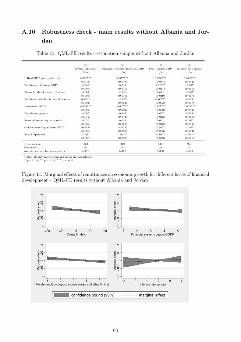
A.10 Robustness check - main results without Albania and Jor-

dan

Table 15: QML-FE results - estimation sample without Albania and Jordan

(1) (2) (3) (4)

Overall fin.cond. Financial systems deposits/GDP Priv. credit/GDP Interest rate spread

b/se b/se b/se b/se

L.Real GDP per capita (log) 0.862*** 0.857*** 0.856*** 0.823***

(0.044) (0.049) (0.047) (0.054)

Remittance inflows/GDP 0.003 0.018 0.023** -0.005

(0.003) (0.015) (0.011) (0.015)

Financial development (findev) 0.001 -0.004 0.002 -0.007

(0.003) (0.030) (0.019) (0.027)

Remittance-findev interaction term -0.001* -0.005 -0.007** 0.003

(0.001) (0.004) (0.003) (0.007)

Investment/GDP 0.008*** 0.007*** 0.007*** 0.009***

(0.002) (0.002) (0.002) (0.002)

Population growth 0.005 0.007 0.007 0.008

(0.012) (0.014) (0.013) (0.015)

Years of secondary education 0.036 0.043 0.041 0.067*

(0.029) (0.028) (0.028) (0.035)

Government expenditure/GDP -0.005* -0.005* -0.005* -0.005

(0.003) (0.003) (0.003) (0.004)

Trade Openness 0.001* 0.001** 0.001** 0.001**

(0.000) (0.000) (0.000) (0.001)

Observations 323 319 318 221

Countries 59 59 59 51

average no. of obs. per country 5.475 5.407 5.390 4.333

Notes: Bootstrapped standard errors in parentheses∗ p < 0.10, ∗∗ p < 0.05, ∗∗∗ p < 0.01

Figure 11: Marginal effects of remittances on economic growth for different levels of financialdevelopment – QML-FE results without Albania and Jordan

−.1

−.0

50

.05

.1M

arg

ina

l e

ffe

ct

−20 −10 0 10 20Overal fin.dev.

−.1

−.0

50

.05

.1M

arg

ina

l e

ffe

ct

1 2 3 4 5Financial systems deposits/GDP

−.1

−.0

50

.05

.1M

arg

ina

l e

ffe

ct

1 2 3 4 5Private credit by deposit money banks and other fin.inst./GDP

−.1

−.0

50

.05

.1M

arg

ina

l e

ffe

ct

−1 0 1 2 3 4Interest rate spread

confidence bound (90%) marginal effect

63