Embed Size (px)
Citation preview

Fit Adequacy of Dichotomous Logit Response Models of the Regressor Bernoulli and Binomial Probability Distributions
Ugwuanyim, G. Uzodinma1, a and Ogbonna, C. Justin1, b* 1Department of Statistics, Federal University of Technology, Owerri, Imo State, Nigeria
[email protected], [email protected]
Keywords: Logit models, Quantal Variables, Base Rate, Goodness-of-fit, Bernoulli distribution, Binomial Distribution.
Abstract: Logit models belong to the class of probability models that determine discrete
probabilities over a limited number of possible outcomes. They are often called ‘Quantal Variables’
or ‘Stimulus and Response Models’ in Biological Literature. The conventional 2R measure of
goodness-of-fit is problematic in logit models. This has therefore led to the proposal of several
alternative goodness-of-fit measures. But researchers in this area have identified the base rate
problem in using these several alternative goodness-of-fit measures. This research is an extension of
work done by people in this area. Specifically, this research is aimed at investigating the goodness-
of-fit performances of eight statistics using the Bernoulli and Binomial distributions as explanatory
variables under various scenarios. The study will draw conclusions on the “best” fit. The data for
the study was generated through simulation and analysed using the multiple correlation analysis.
The findings clearly show that for the Bernoulli Distribution, the goodness-of-fit statistics to use
are: 2 2 2, ,o C M pR R R and ; and for the Binomial Distribution, the goodness-of-fit statistics to use are:
2
NR and p . 2
oR stood out as the “best” goodness-of-fit statistics.
1.0. Introduction
Logit models belong to the class of probability models that determine discrete probabilities over a
limited number of possible outcomes [1]. Like the OLS regression model, the logit model permits
of all sorts of extensions and of quite sophisticated variants. Logit models are often called ‘Limited
Dependent Variable Models’ or ‘Qualitative or Categorical Response Models’ in Econometrics;
‘Quantal Variables’ or ‘Stimulus and Response Models’ in Biological Literature; ‘Discrete Choice’
in Psychology and Economics [1]. When the response takes one of only two possible values
representing success and failure, or more generally the presence or absence of an attribute of
interest, we say that it is binary or dichotomous; but if the response variable can have more than two
outcomes, then, we say that it is polytomous. In this category, if the response variable is ordered, it
gives rise to ordered logit or probit (ologit or oprobit) models; otherwise, it gives rise to
multinomial logit or multinomial probit models [2].
Originally, only researchers from medical disciplines (especially epidemiology)used this form of
regression. More recently, however, logistic regression has been discovered by those who conduct
empirical investigations in a wide array of disciplines. Its popularity continues to grow at such a
rate that it may soon overtake multiple regression and become the most frequently used regression
tool of all [3]. For instance, the Logit model has been used extensively in analyzing growth
phenomena, such as population, GNP, money supply, etc. [2]. It is now commonly used in many
disciplines; for example, in health-sciences research, particularly in medical sciences and
engineering settings. It is also becoming increasingly popular in the behavioural and social sciences
as it is an important endpoint in quality control and quality testing [4].
Historically, the roots of the logit model spread back to the 19th century, when the function was
invented to describe population growth and given its name by the Belgian mathematician Verhulst.
The rediscovery of the growth function is due to Pearl and Reed, the survival of the term logistic to
Yule, and the introduction of the function in bio-assay (and hence in statistics in general) to
Berkson[5].
Bulletin of Mathematical Sciences and Applications Submitted: 2016-03-29ISSN: 2278-9634, Vol. 16, pp 38-48 Accepted: 2016-07-06doi:10.18052/www.scipress.com/BMSA.16.38 Online: 2016-08-042016 SciPress Ltd, Switzerland
SciPress applies the CC-BY 4.0 license to works we publish: https://creativecommons.org/licenses/by/4.0/

In this study, the dichotomous logit model is studied since by far, the ‘most widely used discrete
choice model is logit’ [6].
The logit model as given in [4] is:
1
1
exp
( ) ;
1 exp
k
o i ij
i
j k
o i ij
i
x
p x
x
j = 1, 2, …, n (1)
where:
( )jp x Pr(Y = 1| X = jx ) = E(Y = 1| X =
jx ) denote the expected probability value of
Y given x
ijx = (1, ,...,oj j kjx x x ) denote the j th setting of values of k explanatory variables,
i = 1, 2, …, k , j = 1, 2, …, n , for which ojx = 1, k is a constant
n = the sample size
i , i = 1, 2, …, k are the model parameters.
In Eq. 1 above, the basic random variable Y is dichotomous response data taking the value 1 with
the success probability P , and the value 0 with the failure probability (1 – P ). Y is therefore
assumed to follow a Bernoulli ( P ) distribution.
One of the uses of Regression Analysis is forecasting. In this case, we are interested in how well
the regression model predicts movements in the dependent variable. A summary measure that tells
us how well the sample regression line fits the data is the 2R Statistic. It is a measure of goodness-
of-fit which measures the proportion or percentage of the total variation in Y (the regressand)
explained by the regression model. It is often measured as the squared correlation between the
observed values of Y and the predictions produced by the estimated regression equation [7].
[7]emphasizes that 2R is a measure of linear association between X (the independent variable) and
Y (the dependent variable). It usually lies in the interval [0, 1].
In ordinary least squares (OLS) regression, there appears to be a general consensus on the use of
the coefficient of determination or explained variance, 2R , as an indicator of model fit for a
quantitative dependent variable. In logistic regression analysis, by contrast, there is as yet no
consensus on how we should calculate corresponding measures of the strength of association
between the dependent variable and the total set of predictors. One reason is because, as described
by Efroncited in [8], there is only one reasonable residual variation criterion for quantitative
dependent variables in OLS, the familiar error sum of squares, 2ˆ( )y y , but there are several
possible residual variation criteria (entropy, squared error, qualitative difference) for binary
dependent variables. Another hindrance to consensus is the existence of numerous mathematical
equivalents to 2R in OLS, which are not necessarily mathematically (same formula) or conceptually
(same meaning in the context of the model) equivalent to 2R in logistic regression. This is probably
why [2] says that in binary regression models, goodness-of-fit models are of secondary importance.
What matters are the expected signs of the regression coefficients and their statistical and/or
practical importance. Also, John Aldrich and Forrest Nelson in [2] contend that “use of coefficient
of determination as a summary statistic should be avoided in models of qualitative dependent
variable”.
Since the conventional 2R measure of goodness-of-fit is problematic in limited variable models
where the predicted values are probabilities and the actual values are either 0 or 1, it is desirable to
generalize the definition of 2R to more general models for which the concept of residual variance
cannot be easily defined and maximum likelihood is the criterion of fit. This has therefore led to the
proposal of several alternative goodness-of-fit measures.
There are two groups of goodness-of-fit statistics used to evaluate the association between the
independent variables and the dependent variable in logistic regression analysis. One group is to
Bulletin of Mathematical Sciences and Applications Vol. 16 39

compare predicted and observed discrete values of the dependent variable, using prediction table
and to classify as errors qualitative differences between the observed and predicted outcomes for
each case (the person, place, or thing on which measurement is being performed) or on each
observation (the measurement that is taken) when there is more than one observation per case.
Such measures, says [8] are called Indexes of Predictive Efficiency and they use an absolute,
qualitative “right or wrong” standard for assessing accuracy of prediction. These indexes are
define𝑑 𝑎𝑠:
1p ii noden f n n (2)
1 ( )p ii i in f f n f n (3)
1p ii iin f n E f (4)
where:
n = sample size
moden = the observed number of cases in the modal category of the dependent variable
ijf = the number of cases observed as having discrete value i and predicted as having discrete
value j
iif = the number of cases for which the predicted value is equal to the observed value
if = the number of cases observed as having discrete value i (i.e., the row sum ( )ijif
where the rows represent observed values and the columns represent predicted values)
( )ijE f = ( ) ( )ij iji jf f n
= the expected cell frequency for any cell
( )iiE f = the expected number of correctly classified cases calculated as the product of the
row sum i and the column sum j divided by the total sample size.
All three indexes have proportional reduction in error interpretations (with negative coefficients
indicating an increase in error, a value of zero indicating no relationship and a value of one
indicating perfect prediction).
Another group is the use of 2R analogs (popularly called ‘pseudo- 2R s’) that compare the
discrete observed values (typically zero and one for a dichotomous dependent variable) with the
continuous predicted values (probabilities) that result from applying the logistic regression
equation. [8]also identifies five of these measures as follows:
2
2
2
ˆ( )1
( )o
y yR
y y
(5)
2 ln( )1
ln( )
MMF
o
LR
L
(6)
2/
2 1
n
oM
M
LR
L
(7)
2/
2
2/
1 ( / )
1 ( )
n
o M
N n
o
L LR
L
(8)
2 MC
M
GR
G n
(9)
40 BMSA Volume 16

where:
Eq. 5 – Eq. 9 are respectively: The Ordinary Least Squares 2R , the Log Likelihood Ratio 2R ,
the Geometric Mean Squared Improvement PerObservation 2R , The Adjusted Geometric
Mean Squared Improvement 2R , and, The Contingency Coefficient 2R . n =total sample size, the number of cases (people, cities, widgets) assuming asingle observation
per case, or the number of observations when there are multiple observations per case (as for
example in discrete event history models with pooled time series and cross-sectional data).
oL =the likelihood function of the model containing only the intercept.
ML =the likelihood function for the model containing all of the predictors.
MG = 2[ln( ) ln( )]o ML L = the model Chi-Square Statistic.
y = the predicted value of the dependent variableY ,obtained from the model, a continuous
probability with a value between 0 and 1.
y =the observed value of the dependent variableY , coded as discrete integer value.
y =the mean value of the dependent variable Y , a continuous probability.
Researchers in this area have identified the base rate problem in using the measures of predictive
efficiency and pseudo- 2R values as goodness-of-fit measures [9], [8], [4]. For instance, [8], in his
study posits that ‘in general, most of the coefficients of determination are so highly correlated with
the base rate that the base rate itself could practically be used as a coefficient of determination’. So,
those statistics that are base-rate invariant are seen to be the “best” measures of goodness-of-fit.
[8]thus recommends future research for a more detailed mathematical analysis to determine the
nature of the relationship of the various 2R analogs and indexes of predictive efficiency with the
base rate. In addition, he adds, simulation research like [9] research on the indices of predictive
efficiency would be useful in studying 2 2 2 2, , ,o MF M NR R R R and 2
CR to examine in more detail their
relationship to the base rate, their behavior in the presence of unreliability of measurement, and the
extent to which the limited result presented in his study may be peculiar to the data he used, or
generalizable to a broader range of data.
[9] define base rate to be ‘the relative frequency of occurrence (i.e., ratio of success to failures) of
the event being studied in the population of interest’. They opine that the base rate problem stems
from the fact that statistical prediction models often are not valid when applied to populations with
a different base rate than the population for which the prediction model was constructed. The
reason for this, they continued, is that the base rate for a dichotomous variable becomes the
marginal distribution of the outcome expectancy table and the computation of the predictive
accuracy index is based on this expectancy table. They give an example that if 40% of students
successfully complete a developmental mathematics program, then, a 40% base rate will be used in
the logistic regression prediction model. But if that same model is then used on a group of
developmental mathematics students representing a population with a true base rate of 20%, then,
many errors in classification will occur since the prediction model will be invalid for the latter
group of students.
Kvalsethcited in [8] stated that one of the eight properties 2R should have is that 2R should be such
that its values for different models fitted to the same dataset are directly comparable. Menard
explained this to mean that the coefficient of determination should be comparable across not only
different predictors but different dependent variables and different subsets of the dataset. An
unknown reviewer cited [8] however, cautions that comparisons of performance across different
datasets make sense only if the explanatory variables have a meaningfully defined distribution. In
response to this remark, [4], carried out a research on the assessment of the ‘adequacy-of-fit of logit
models’ under the dichotomous response classified by its probability levels using the Exponential,
Bernoulli and Multinomial distributed explanatory variables. They used a single sample size of 200
and a single replication size of 1000 in their study. Their study does not give the “best” goodness-
of-fit statistics among the studied statistics but they recommend that ‘further studies for more details
in the exponential explanatory distribution together with increased sample sizes’ be carried out.
Bulletin of Mathematical Sciences and Applications Vol. 16 41

This research is, therefore, an extension of the work of [4] and further investigates the goodness-of-
fit performances of the eight statistics of equations (2) – (9) using the Bernoulli and Binomial
distributions as explanatory variables by investigating the effect of base rates on the performances
of these statistics under variable conditions of sample sizes, replications and parameter values for
stability of results. The study also draws conclusions on the “best” fit.
2.0. Literature Review
[9] used Monte Carlo Simulation methods to investigate how the three indices of predictive
efficiency in equations (2), (3) and (4) as well as frequently used Relative Improvement Over
Chance (RIOC) and the Percentage Correct Classification Indices would be influenced by
fluctuations in the base rate given various constraints, namely, changes in measurement reliability
levels of predictor variables, changes in sample size and changes in the selection ratio of the logistic
regression model. In their finding, they say that p is the most base rate invariant index if the model
comprised of one continuous and one dichotomous predictor;p is the most base rate invariant
index if the model comprised of two dichotomous variables, while for either model, p is almost the
most sensitive to base rate changes. They recommended that future research should investigate
these same indices for base rate influence within other designs of logistic regression models, for, it
is possible that there are other predictor variable combinations which alter the patterns of the index
means. They insisted that the search for a base rate invariant predictive efficiency index continues
for as long as model conditions dictate the appropriateness of an index for assessing efficiency,
ambiguity will continue to exist regarding which index to use, and when to use it.
Again, in his study of ‘Coefficients of Determination for Multiple Logistic Regression Analysis’,
[8] discovered that 2
MFR seems preferable to the other 2R analogs in two respects. Firstly, 2
MFR has
the most intuitive reasonable interpretation as a proportional reduction in error measure, parallel to2
oR . Secondly, 2
MFR stands out for its independence from the base rate, relative to other 2R analogs.
He also says, with regard to his study, with a manipulated base rate but no constraints on the
selection ratio, p also stands out for its relative independence from the base rate. This contradicts
with the findings of [9] mentioned in the preceding paragraph that p is the best index of predictive
efficiency given that both the base rate and the selection ratio are fixed. [8] definesselection ratioas
the proportion of cases for which y = 1, and is of concern only when some fixed proportion of
cases is in some sense “selected” as successes or equivalently, when the threshold or “cut point” for
classification is fixed at some value other than the usual expected value of 1/k, where k is the
number of categories in the dependent variable. [8] thus recommends that future researches
undertake both a more detailed mathematical analysis to determine the nature of the relationship of
the various 2R analogs and indexes of predictive efficiency with the base rate. In addition, he goes
on to say that simulation research like [9]work on the indices of predictive efficiency would be
useful in studying 2 2 2 2, , ,o MF M NR R R R and 2
CR to examine in more detail their relationship to the base
rate, their behavior in the presence of unreliability of measurement, and the extent to which the
limited result presented in his study may be peculiar to the data he used, or generalizable to a
broader range of data.
In line with the two works cited above, [4], carried out a research on the assessment of the
‘adequacy-of-fit of logit models’ under the dichotomous response classified by its probability levels
using the Exponential, Bernoulli and Multinomial distributed explanatory variables. Their findings
show that the coefficients of correlation between 2R analogs and base rate levels of exponential-
distributed X s indicate that the 2 2,C MR R and 2
oR statistics are most useful in terms of smaller values of
their correlation coefficients with the base rate levels. Also, the results of the correlation
coefficients between the indexes of predictive efficiency and base rate levels of the exponential
42 BMSA Volume 16

distribution show that the statistics,p and
p have better performance than the p statistics. This
is contrary to the findings of [8] cited above probably because Menard (2000) used only categorical
predictors in his work. The findings agree more with [9] also cited above who say that p is the
most base rate invariant index if the model comprised of one continuous and one dichotomous
predictor;p is the most base rate invariant index if the model comprised of two dichotomous
variables; while for either model, p is almost the most sensitive to base rate changes. [4]results
further show that for the Bernoulli and Multinomial independent variable models, the correlation
coefficients are approximately the same for the 2R analogs and ‘most values’ tend to be more
independent from base rates than those of the exponential distribution. Furthermore, the results of
the correlation coefficients between the indexes of predictive efficiency and base rate levels show
that p and
p are better than p . This also agrees partly with the work of [9] who posit that
p is
the most base rate invariant index if the model comprised of two dichotomous variables, and partly
with the work of [8]. Finally, [4] recommend the use of2 2 2, , ,C M o pR R R and
p as goodness-of-fit
measures for logit models with dichotomous response and exponential explanatory variables. They,
however, say that when P is close to 0.5, the percentage correct is low and the range is high for the
exponential response model. They thus recommend that ‘further studies for more details in the
exponential explanatory distribution together with increased sample sizes’ be carried out.
[10, 11, 12], [13], [14] and [15] all investigated the properties of various pseudo-R2s using Monte
Carlo Experiments. These studies conducted simulations to determine how closely most of the
Pseudo-R2s correspond to the OLS-R
2 on the underlying latent variable model. This paper does not
use this approach but rather the approach specified in section 1.
3.0. Methodology
This paper is a comparative study of the performances of some goodness-of-fit statistics under
various scenarios. The Monte Carlo Simulation (Experimentation) method is used to generate the
data. The simulation study is undertaken using a sample size of 100, 200 and 500; a replication size
of 1000, 2000 and 5000 for stability of results. The base rates are: 0.20, 0.35, 0.50 and 0.65. The
analyses are carried out using the multiple correlation method. The correlation coefficients will
indicate which of the goodness-of-fit measures are correlated under the base rates, sample sizes,
replications and parameter values criteria. Any goodness-of-fit measure that is not correlated under
the above criteria are seen in this sense as a good measure of goodness-of-fit. For ease of
interpretation, the results of the analyses are ranked. Ranks are used to find out the “best” statistics
and the most variable of the studied probability distributions. “Best” in this study is used to
indicate the goodness-of-fit statistics that is most invariant to the base rate and any of the goodness-
of-fit statistics that has the least total rank under the studied scenarios is considered as the “best”
statistics. The coefficient of variation is used to find the variability of the distributions. Any of the
probability distributions that has the highest total variability rank for all the studied statistics is seen
as the most variable probability distribution.
All the analyses are carried out using STATA 12.0. The hypothesis of significant correlation
coefficients was tested at 5% level of significance and the significant correlation coefficients at this
level of significance are marked with asterisk (*). The Monte Carlos Simulation program was also
written with STATA 12.0 and attached to this paper as Appendix.
3.1. Description of the Simulation Study.In this section, we explain how each simulation was
carried out. In addition to the sample sizes, replications and base rate values:
3.1.1 The Bernoulli Distribution is studied under the following parameter values: 0.10,
0.30 and 0.45. In all, 108 simulations were carried out under the Bernoulli distribution.
Bulletin of Mathematical Sciences and Applications Vol. 16 43
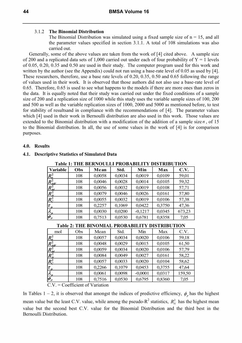
3.1.2 The Binomial Distribution The Binomial Distribution was simulated using a fixed sample size of n = 15, and all
the parameter values specified in section 3.1.1. A total of 108 simulations was also
carried out.
Generally, some of the above values are taken from the work of [4] cited above. A sample size
of 200 and a replicated data sets of 1,000 carried out under each of four probability of Y = 1 levels
of 0.05, 0.20, 0.35 and 0.50 are used in their study. The computer program used for this work and
written by the author (see the Appendix) could not run using a base-rate level of 0.05 as used by [4].
These researchers, therefore, use a base rate levels of 0.20, 0.35, 0.50 and 0.65 following the range
of values used in their work. It is observed that those authors did not also use a base-rate level of
0.65. Therefore, 0.65 is used to see what happens to the models if there are more ones than zeros in
the data. It is equally noted that their study was carried out under the fixed conditions of a sample
size of 200 and a replication size of 1000 while this study uses the variable sample sizes of 100, 200
and 500 as well as the variable replication sizes of 1000, 2000 and 5000 as mentioned before, to test
for stability of resultsand in compliance with the recommendations of [4]. The parameter values
which [4] used in their work in Bernoulli distribution are also used in this work. Those values are
extended to the Binomial distribution with a modification of the addition of a sample size n , of 15
to the Binomial distribution. In all, the use of some values in the work of [4] is for comparison
purposes.
4.0. Results
4.1. Descriptive Statistics of Simulated Data
Table 1: THE BERNOULLI PROBABILITY DISTRIBUTION
Variable Obs Mean Std. Min Max C.V.
108 0,0058 0,0034 0,0019 0,0109 59,01
108 0,0046 0,0028 0,0014 0,0105 59,32
108 0,0056 0,0032 0,0019 0,0108 57,71
108 0,0079 0,0046 0,0026 0,0161 57,80
108 0,0055 0,0032 0,0019 0,0106 57,38
108 0,2257 0,1069 0,0422 0,3750 47,36
108 0,0030 0,0200 -0,1217 0,0345 673,23
108 0,7513 0,0530 0,6781 0,8358 7,05
2
0R2
MFR2
MR2
NR2
CR
p
p
p
2
0R2
MFR2
MR2
NR2
CR
p
p
p
Table 2: THE BINOMIAL PROBABILITY DISTRIBUTION
mol Obs Mean Std. Min Max C.V.
108 0,0057 0,0034 0,0020 0,0106 59,18
108 0,0048 0,0029 0,0015 0,0105 61,50
108 0,0059 0,0034 0,0020 0,0106 57,79
108 0,0084 0,0049 0,0027 0,0161 58,22
108 0,0057 0,0033 0,0020 0,0104 58,62
108 0,2266 0,1079 0,0453 0,3755 47,64
108 0,0061 0,0098 -0,0001 0,0317 159,50
108 0,7516 0,0530 0,6795 0,8360 7,05
2
0R2
MFR2
MR2
NR2
CR
p
p
p
2
0R2
MFR2
MR2
NR2
CR
p
p
p C.V. = Coefficient of Variation
In Tables 1 – 2, it is observed that amongst the indices of predictive efficiency, p has the highest
mean value but the least C.V. value, while among the pseudo-R2 statistics, 2
NR has the highest mean
value but the second best C.V. value for the Binomial Distribution and the third best in the
Bernoulli Distribution.
44 BMSA Volume 16

4.2. ANALYSES OF SIMULATED DATA
Table 3: EFFECT OF BASE-RATE ON GOODNESS-OF-FIT MEASURES AT VARIOUS
VALUES OF n, REPLICATIONS AND PARAMETER VALUES FOR THE BERNOULLI
DISTRIBUTION CORRELATION COEFFICIENTS.
Table 3 gives one the general summary of the effect of base-rate on the goodness-of-fit measures at
various values of n, replications and parameter values (p).
(a) At various values of n, 2
oR is base-rate invariant. It is also independent of replications and
parameter values.
(b) 2
MR is independent of the base rate at sample sizes of 200 and 500. It is also independent of
the base rate at all replications and parameter values.
(c) 2
CR is independent of the base rate at sample sizes of 200 and 500 as well as all replications
and parameter values.
(d) p is uncorrelated with the base rate at the sample size of 500 and parameter value of 0.3.
Therefore thefollowing statistics are good for the Bernoulli Distribution: 2
oR , 2
MR , 2
CR and p ; and
2
NR at n = 100.
Table 4: EFFECT OF BASE-RATE ON GOODNESS-OF-FIT MEASURES AT VARIOUS
VALUES OF N, REPLICATIONS AND PARAMETER VALUES FOR THE BINOMIAL
DISTRIBUTION CORRELATION COEFFICIENTS.
(a) Base-rate is independent of the goodness-of-fit statistics at only the sample size, n, of 500 of 2
NR andp . All the other statistics are correlated with the base rate at the various sample
sizes under consideration.
(b) Base-rate is independent of all the pseudo-R2 statistics at all the replication values; it is not
also correlated with p at a replication value of 5,000.
(c) Base-rate is not correlated with the goodness-of-fit statistics at the considered parameter
values for all the pseudo-R2 statistics and
p at only the parameter values of 0.10 and 0.30.
Bulletin of Mathematical Sciences and Applications Vol. 16 45

It therefore indicates that 2
NR is the best pseudo- R2 statistics to use at the sample size of 500 and all
replication and parameter values. p is the best index of predictive efficiency statistics at the sample
size of 500, replication value of 5,000 and parameter values of 0.10 and 0.30.
Table 5: RANKS FOR FINDING THE “BEST” STATISTICS
Table 5 indicates that 2
oR with a total rank of 32 stands out as the “best” statistics. This is followed
by 2
CR and 2
MR in this order.
5.0. Conclusion
The findings of this paper clearly show that:For the Bernoulli Distribution,
(a) At various values of n, 2
oR is base-rate invariant. It is also independent of replications and
parameter values.
(b) 2
MR is independent of the base rate at sample sizes of 200 and 500. It is also independent of
the base rate at all replications and parameter values.
(c) 2
CR is independent of the base rate at sample sizes of 200 and 500 as well as all replications
and parameter values.
(d) p is uncorrelated with the base rate at the sample size of 500 and parameter value of 0.3.
For the Binomial Distribution,
(e) Base-rate is independent of the goodness-of-fit statistics at only the sample size, n, of 500 of 2
NR andp . All the other statistics are correlated with the base rate at the various sample
sizes under consideration.
(f) Base-rate is independent of all the pseudo-R2 statistics at all the replication values; it is not
also correlated with p at a replication value of 5,000.
(g) Base-rate is not correlated with the goodness-of-fit statistics at the considered parameter
values for all the pseudo-R2 statistics and
p at only the parameter values of 0.10 and 0.30.
In addition,
(h) 2
oR with a total rank of 32 stands out as the “best” statistics. This is followed by 2
CR and 2
MR
in this order.
(i) p was found not only to yield the highest estimates of predictive efficiency regardless of
base rate, sample size or replication conditions, but yielded the least variation among the
studied statistics.
(j) p consistently yielded the lowest and the most variable estimates of predictive efficiency
regardless of base rate, sample size, replication and parameter value conditions
(k) 2
MFR ,p and
p are not invariant to the base rate contrary to the findings of [8] and [9].
(l) The finding that 2
oR , 2
CR and 2
MR as good goodness-of-fit statistics in the Bernoulli
Distribution is in agreement with the work of [4].
VARIABLE BERNOULLI BINOMIAL GRAND TOTAL POSITION
16 16 32 1
49 54 103 6
21 31 52 3
35 34 69 4
26 22 48 2
59 58 117 7
49 42 91 5
69 67 136 8
46 BMSA Volume 16

APPENDIX
Here, we use one example of a Binomial Distribution with n = 15, p = 0.45 and a Bernoulli
Distribution with a base-rate of 0.65 as follows:
set more off
clear all
set seed 10101
postfile uz1 ro2 rl2 rm2 rn2 rc2 lambda_ptau_pphi_p using uzo1results, replace
forvalues i = 1/1000 {
drop _all
setobs 100
gen x1 = rbinomial(15, 0.45)
gen y1 = rbinomial(1, 0.65)
quietlylogit y1 x1
predict y2, pr
gen n = e(N)
gen c = e(ll)
gen d = e(ll_0)
gen y3 = (y1-y2)^2
egen y4 = mean(y1)
gen y5 = (y1-y4)^2
egen y6 = total(y3)
egen y7 = total(y5)
gen m = c-d
gen b = (-2/n)*m
gen z1 = exp(b)
gen z2 = (2/n)*d
gen z3 = exp(z2)
gen z4 = 1 - z3
gen ro2 = 1-(y6/y7)
gen rmf2 = 1 - c/d
gen rm2 = 1 - z1
gen rn2 = (rm2)/z4
gen rc2 = -2*(d-c)/(-2*(d-c) + n)
gen y8 = 1 if y2 > 0.5
replace y8 = 0 if y2 <= 0.5
rename y8 yhat
tab y1 yhat
gen y9 = 1 if y1 ==1 &yhat==1
gen y10 = 1 if y1 ==0 &yhat==0
gen y11 = 1 if y1 ==1 &yhat==0
gen y12 = 1 if y1 ==0 &yhat==1
egen mode = mode(y1), maxmode
gen y_1 = mode if y1 == mode
egenn_mode = count(y_1)
egen totaly9 = total(y9)
egen totaly10 = total(y10)
egen totaly11 = total(y11)
egen totaly12 = total(y12)
Bulletin of Mathematical Sciences and Applications Vol. 16 47
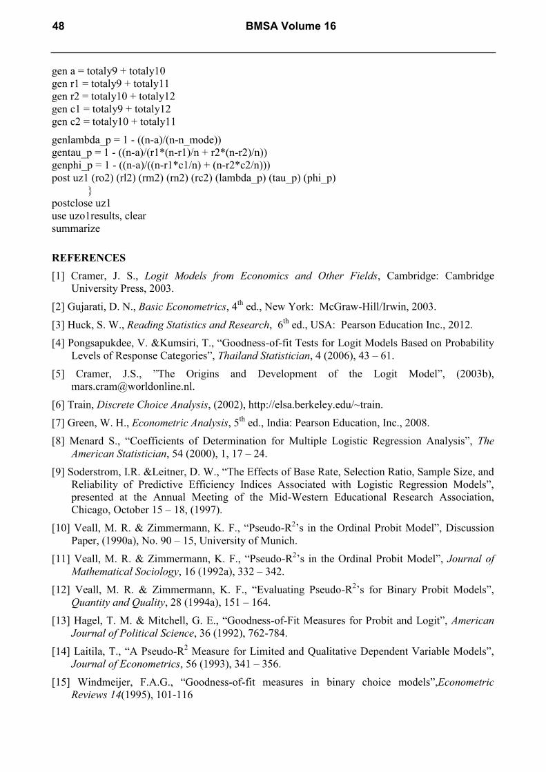
gen a = totaly9 + totaly10
gen r1 = totaly9 + totaly11
gen r2 = totaly10 + totaly12
gen c1 = totaly9 + totaly12
gen c2 = totaly10 + totaly11
genlambda_p = 1 - ((n-a)/(n-n_mode))
gentau_p = 1 - ((n-a)/(r1*(n-r1)/n + r2*(n-r2)/n))
genphi_p = 1 - ((n-a)/((n-r1*c1/n) + (n-r2*c2/n)))
post uz1 (ro2) (rl2) (rm2) (rn2) (rc2) (lambda_p) (tau_p) (phi_p)
}
postclose uz1
use uzo1results, clear
summarize
REFERENCES
[1] Cramer, J. S., Logit Models from Economics and Other Fields, Cambridge: Cambridge
University Press, 2003.
[2] Gujarati, D. N., Basic Econometrics, 4th
ed., New York: McGraw-Hill/Irwin, 2003.
[3] Huck, S. W., Reading Statistics and Research, 6th
ed., USA: Pearson Education Inc., 2012.
[4] Pongsapukdee, V. &Kumsiri, T., “Goodness-of-fit Tests for Logit Models Based on Probability
Levels of Response Categories”, Thailand Statistician, 4 (2006), 43 – 61.
[5] Cramer, J.S., ”The Origins and Development of the Logit Model”, (2003b),
[6] Train, Discrete Choice Analysis, (2002), http://elsa.berkeley.edu/~train.
[7] Green, W. H., Econometric Analysis, 5th
ed., India: Pearson Education, Inc., 2008.
[8] Menard S., “Coefficients of Determination for Multiple Logistic Regression Analysis”, The
American Statistician, 54 (2000), 1, 17 – 24.
[9] Soderstrom, I.R. &Leitner, D. W., “The Effects of Base Rate, Selection Ratio, Sample Size, and
Reliability of Predictive Efficiency Indices Associated with Logistic Regression Models”,
presented at the Annual Meeting of the Mid-Western Educational Research Association,
Chicago, October 15 – 18, (1997).
[10] Veall, M. R. & Zimmermann, K. F., “Pseudo-R2’s in the Ordinal Probit Model”, Discussion
Paper, (1990a), No. 90 – 15, University of Munich.
[11] Veall, M. R. & Zimmermann, K. F., “Pseudo-R2’s in the Ordinal Probit Model”, Journal of
Mathematical Sociology, 16 (1992a), 332 – 342.
[12] Veall, M. R. & Zimmermann, K. F., “Evaluating Pseudo-R2’s for Binary Probit Models”,
Quantity and Quality, 28 (1994a), 151 – 164.
[13] Hagel, T. M. & Mitchell, G. E., “Goodness-of-Fit Measures for Probit and Logit”, American
Journal of Political Science, 36 (1992), 762-784.
[14] Laitila, T., “A Pseudo-R2 Measure for Limited and Qualitative Dependent Variable Models”,
Journal of Econometrics, 56 (1993), 341 – 356.
[15] Windmeijer, F.A.G., “Goodness-of-fit measures in binary choice models”,Econometric
Reviews 14(1995), 101-116
48 BMSA Volume 16