Fısica de Neutrinos

A. Mondragon y E. Peinado

Escuela de Fısica Nuclear 2007

Contenido

Primera Parte

• Oscilaciones de los neutrinos entre estados del sabor

• Observaciones y Experimentos

• Breve recordatorio de la Teorıa: Modelo Estandar

• Neutrinos de Dirac y Majorana

• El mecanismo del subibaja (seesaw)

Segunda Parte

• Neutrinos en la Extension S3-invariante del Modelo Estandar

• Las corrientes neutras que cambian el sabor

1

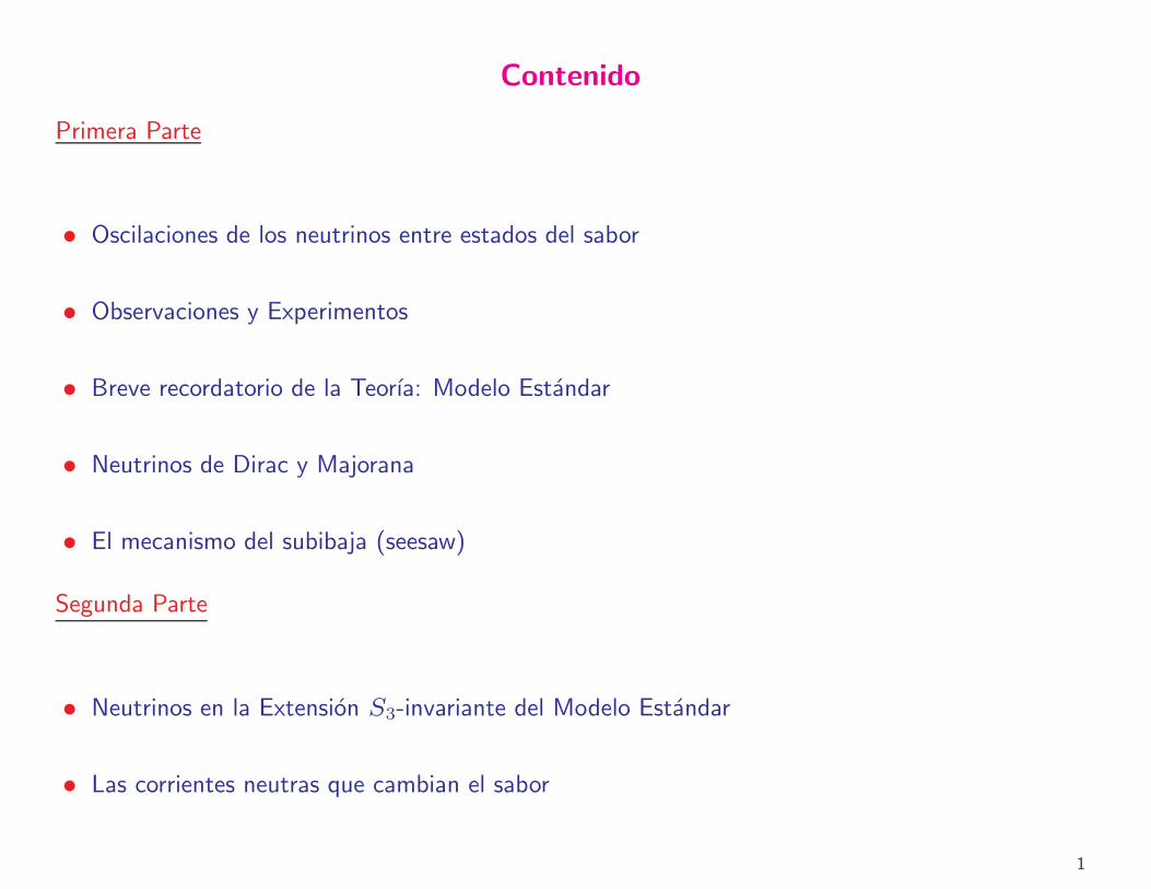
NEUTRINOS

Masas, mezclas de sabores y oscilaciones de los neutrinos

1957 Pontecorvo discutio las oscilaciones ν ↔ ν

1962 Maki, Nakagawa y Sakata propusieron las ”Transiciones virtuales” νe ↔ νµ

1964-1968 Davies observo el deficit de νe solares

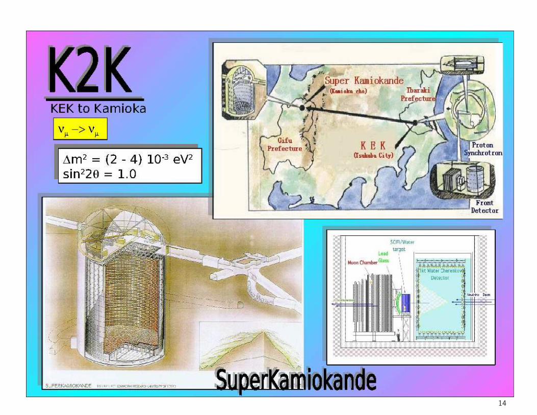
1998 Oscilaciones de los neutrinos νµ atmosfericos

(SuperKamiokande)

2000 Observacion directa de ντ en el experimento DONUT

2001 SNO mide las oscilaciones de los neutrinos νe solares y el flujo total de neutrinos

provenientes del Sol

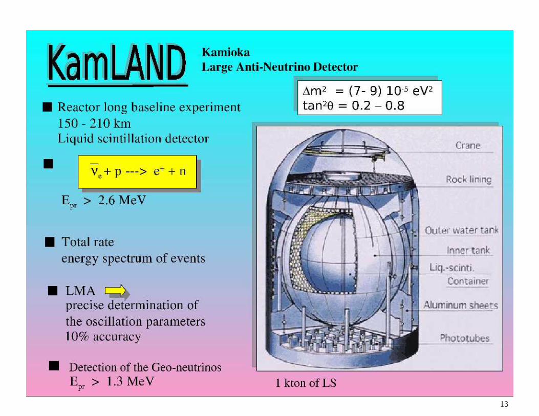
2003 KAMLAND mide los parametros de la oscilacion de los neutrinos νe solares y los de

la oscilacion de los νe de reactores

2003-2007 Se midieron las diferencias de los cuadrados de las masas ∆m2νi,νj

y los angulos

de mezcla en las oscilaciones de los neutrinos entre estados del sabor y se refinaron las cotas

sobre la suma de las masas de los neutrinos con las medidas cosmologicas de presicion.

ESTA ES LA EVIDENCIA EXPERIMENTAL INCONTROVERTIBLE DE FISICA NUEVA

MAS ALLA DEL MODELO STANDARD !!

2

3

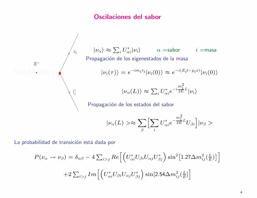
Oscilaciones del sabor

να

l+α

W+

|να〉 ≈P

iU∗αi|νi〉 α =sabor i =masa

Propagacion de los eigenestados de la masa

|νi(τ)〉 = e−imiτi|νi(0)〉 ≈ e−i(Eit−pix)|νi(0)〉

|να(L)〉 ≈P

iU∗αie−im

2i

2EL|νi〉

Propagacion de los estados del sabor

|να(L) >≈X

β

hX

i

U∗αie−m

2i

2ELUβii

|νβ >

La probabilidad de transicion esta dada por

P (να → νβ) = δαβ − 4P

i>j Reh“

U∗αiUβiUαjU∗βj

”

sin2ˆ

1.27∆m2ij(

LE)˜

i

+2P

i>j Imh“

U∗αiUβiUαjU∗βj

”

sin[2.54∆m2ij(

LE ]i

4

5

6

7

8

9

10

11

12

13

14

Grupo de Norma del Modelo Standard

SUc(3) ⊗ SUW (2) ⊗ UY (1)

⇑ ⇑ ⇑

fuerte debil electromagnetica

Los campos fermionicos se describen por sus componentes de quiralidad izquierda o derecha

ψL,R =1

2(1 ± γ5)ψ, ψL,R = ψ(1± γ5)

1

2

QILi(3, 2)+1/6, uRi(3, 1)+2/3, dRi(3, 1)−1/3, L

ILi(1, 2), lRi(1, 1)

sabor, color, isospin debil, hipercarga

En el Modelo Standard hay un campo escalar llamado el campo de Higgs

φ(1, 2)+1/2

15

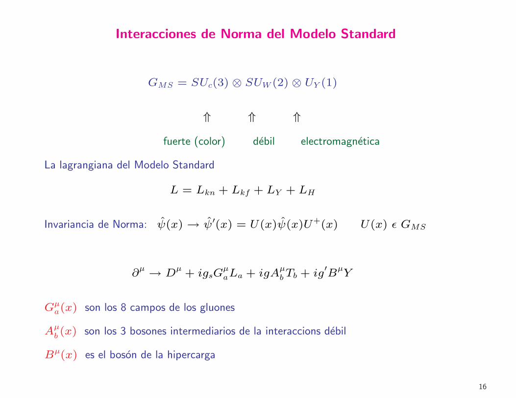
Interacciones de Norma del Modelo Standard

GMS = SUc(3) ⊗ SUW (2)⊗ UY (1)

⇑ ⇑ ⇑

fuerte (color) debil electromagnetica

La lagrangiana del Modelo Standard

L = Lkn + Lkf + LY + LH

Invariancia de Norma: ψ(x)→ ψ′(x) = U(x)ψ(x)U+(x) U(x) ǫ GMS

∂µ → D

µ+ igsG

µaLa + igA

µbTb + ig

′BµY

Gµa(x) son los 8 campos de los gluones

Aµb (x) son los 3 bosones intermediarios de la interaccions debil

Bµ(x) es el boson de la hipercarga

16

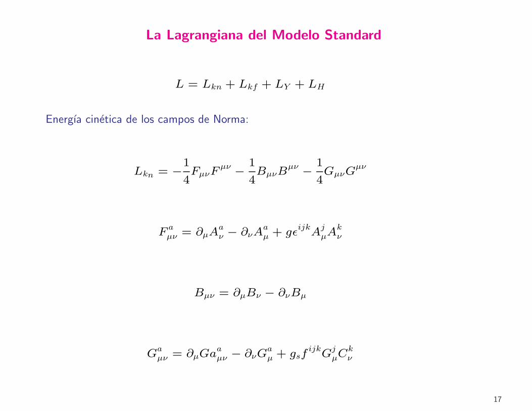
La Lagrangiana del Modelo Standard

L = Lkn + Lkf + LY + LH

Energıa cinetica de los campos de Norma:

Lkn = −1

4FµνF

µν − 1

4BµνB

µν − 1

4GµνG

µν

Faµν = ∂µA

aν − ∂νA

aµ + gǫ

ijkAjµA

kν

Bµν = ∂µBν − ∂νBµ

Gaµν = ∂µGa

aµν − ∂νG

aµ + gsf

ijkGjµC

kν

17

La Lagrangiana de los fermiones

Lkf =X

i

¯iψ+γµDµψ

+i

Dµ

= ∂µ

+ igsGµaLa + igA

µbTb + ig

′Bµ(x)Y

Lagrangiana del campo de Higgs

LH = (Dµφ)†(Dµφ)− V (φ

+φ)

φ(x) =1√

2

n

h(x)12×2 + iwα(x)σαo

Dµφ(x) =“

∂µ −i

2g~τ · ~Aµ −

i

2g′Bµ

”

φ

V (φ) = −µ2φ

+φ+ λ(φ

+φ)

2

18

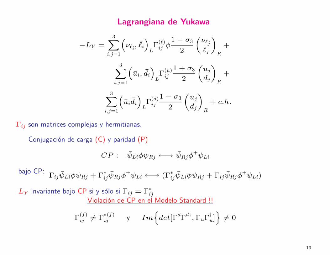
Lagrangiana de Yukawa

−LY =

3X

i,j=1

“

νℓi, ℓi”

LΓ

(ℓ)ij φ

1− σ3

2

„

νℓjℓj

«

R

+

3X

i,j=1

“

ui, di”

LΓ

(u)ij

1 + σ3

2

„

ujdj

«

R

+

3X

i,j=1

“

uidi”

LΓ

(d)ij

1− σ3

2

„

ujdj

«

R

+ c.h.

Γij son matrices complejas y hermitianas.

Conjugacion de carga (C) y paridad (P)

CP : ψLiφψRj ←→ ψRjφ+ψLi

bajo CP:ΓijψLiφψRj + Γ

∗ijψRjφ

+ψLi ←→ (Γ

∗ijψLiφψRj + ΓijψRjφ

+ψLi)

LY invariante bajo CP si y solo si Γij = Γ∗ijViolacion de CP en el Modelo Standard !!

Γ(f)ij 6= Γ

∗(f)ij y Im

n

det[ΓdΓd†,ΓuΓ

†u]o

6= 0

19

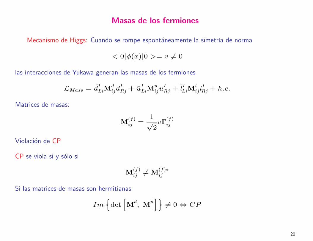
Masas de los fermiones

Mecanismo de Higgs: Cuando se rompe espontaneamente la simetrıa de norma

< 0|φ(x)|0 >= v 6= 0

las interacciones de Yukawa generan las masas de los fermiones

LMass = dILiMdijd

IRj + uILiM

uiju

IRj + l

ILiM

l

ijlIRj + h.c.

Matrices de masas:

M(f)ij =

1√

2vΓ

(f)ij

Violacion de CP

CP se viola si y solo si

M(f)ij 6= M

(f)∗ij

Si las matrices de masas son hermitianas

Imn

deth

Md, M

uio

6= 0⇔ CP

20

Los Neutrinos en el Modelo Estandar

En el Modelo Estandar

• Las masas de los quarks y los leptones cargados se generan en los sectores de Higgs y de Yukawa

• Los neutrinos no tienen masa

• El sector de Yukawa tiene demasiados parametros libres (13)

Por lo tanto, debemos extender la teorıa, con el objetivo de

• Dar masa a los neutrinos

• Sistematizar la fenomenologıa tan rica de las masas y mezclas de los fermiones

• Reducir el numero de parametros

En las Extensiones del Modelo Standard

• Extendimos el concepto del sabor y generacion al sector de Higgs

• Introdujimos una simetrıa permutacional del sabor en el sector de las masas

• Generamos las masas de los neutrinos con el mecanismo del subibaja

21

Neutrinos de Dirac y Neutrinos de Majorana I

Espinores de Dirac

iγµ∂µψ −mψ = 0.

Lagrangiana de Dirac

LD = iψγλ∂λψ −mψψ

Relacion de energıa y momento

pλpλ = m

2

ψ es un espinor de cuatro componentes

γµ son las matrices de Dirac

Neutrinos de Dirac 6= Antineutrinos de Dirac

22

Neutrinos de Dirac y Neutrinos de Majorana II

Espinores de Majorana

La carga electrica de los neutrinos es nula

Si el campo espinorial = al campo conjugado de carga

ψM = ψcM = Cψ

T

C es la matriz de conjugacion de carga

ψM =

„

ν

iσ2ν∗

«

ψM es un espinor de Majorana y tiene solo dos componentes

Neutrinos de Majorana = Antineutrinos de Majorana

23

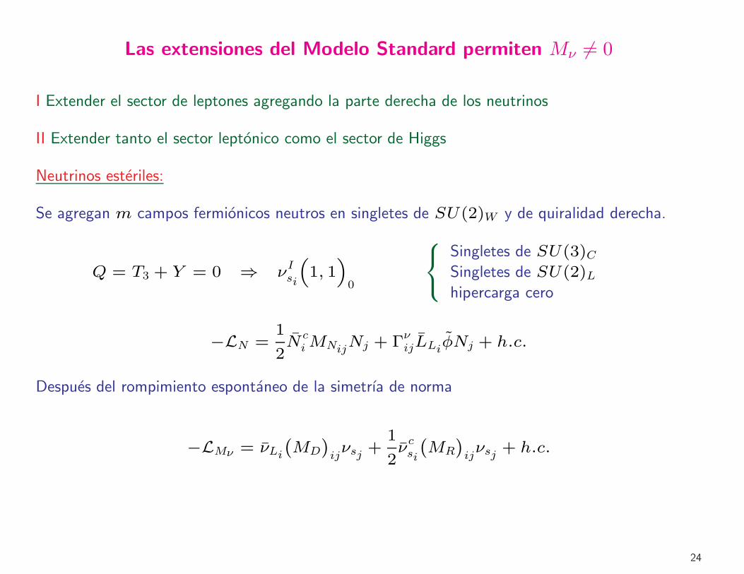
Las extensiones del Modelo Standard permiten Mν 6= 0

I Extender el sector de leptones agregando la parte derecha de los neutrinos

II Extender tanto el sector leptonico como el sector de Higgs

Neutrinos esteriles:

Se agregan m campos fermionicos neutros en singletes de SU(2)W y de quiralidad derecha.

Q = T3 + Y = 0 ⇒ νIsi

“

1, 1”

0

8

<

:

Singletes de SU(3)CSingletes de SU(2)Lhipercarga cero

−LN =1

2NciMNij

Nj + ΓνijLLiφNj + h.c.

Despues del rompimiento espontaneo de la simetrıa de norma

−LMν = νLi`

MD

´

ijνsj +

1

2νcsi

`

MR

´

ijνsj + h.c.

24

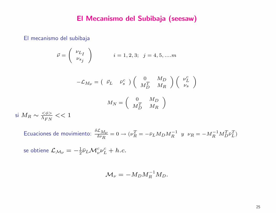
El Mecanismo del Subibaja (seesaw)

El mecanismo del subibaja

~ν =

νLIνsj

!

i = 1, 2, 3; j = 4, 5, ....m

−LMν =`

~νL νcs´

„

0 MD

MTD MR

«„

νcLνs

«

MN =

„

0 MD

MTD MR

«

si MR ∼ <φ>ΛFN

<< 1

Ecuaciones de movimiento:δLMνδνR

= 0→ (νTR = −νLMDM−1R y νR = −M−1

R MTDν

TL )

se obtiene LMν = −12νLM

cνν

cL + h.c.

Mν = −MDM−1R MD.

25

26

Contents

• Flavour permutational symmetry

• A minimal S3-invariant extension of the Standard Model

• Masses and mixings in the leptonic sector

• The neutrino mass spectrum

• FCNCs

• Summary and conclusions

27

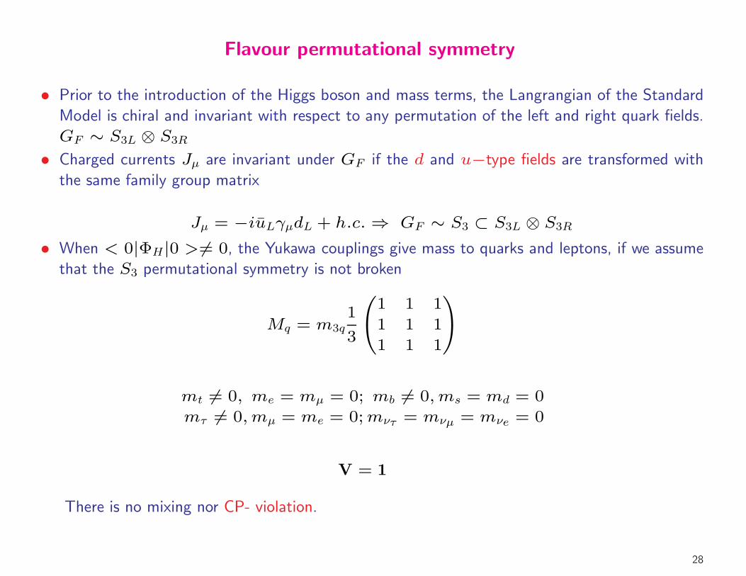
Flavour permutational symmetry

• Prior to the introduction of the Higgs boson and mass terms, the Langrangian of the Standard

Model is chiral and invariant with respect to any permutation of the left and right quark fields.

GF ∼ S3L ⊗ S3R

• Charged currents Jµ are invariant under GF if the d and u−type fields are transformed with

the same family group matrix

Jµ = −iuLγµdL + h.c.⇒ GF ∼ S3 ⊂ S3L ⊗ S3R

• When < 0|ΦH|0 > 6= 0, the Yukawa couplings give mass to quarks and leptons, if we assume

that the S3 permutational symmetry is not broken

Mq = m3q

1

3

0

@

1 1 1

1 1 1

1 1 1

1

A

mt 6= 0, me = mµ = 0; mb 6= 0,ms = md = 0

mτ 6= 0,mµ = me = 0;mντ = mνµ = mνe = 0

V = 1

There is no mixing nor CP- violation.

28

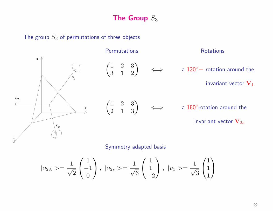
The Group S3

The group S3 of permutations of three objects

Permutations Rotations3

1

2

V2A

V2s

V1

„

1 2 3

3 1 2

«

⇐⇒ a 120◦− rotation around the

invariant vector V1

„

1 2 3

2 1 3

«

⇐⇒ a 180◦rotation around the

invariant vector V2s

Symmetry adapted basis

|v2A >=1√2

0

@

1

−1

0

1

A , |v2s >=1√6

0

@

1

1

−2

1

A , |v1 >=1√3

0

@

1

1

1

1

A

29

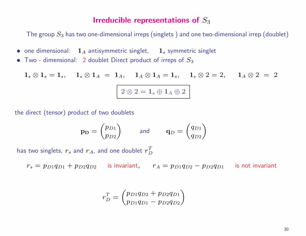
Irreducible representations of S3

The group S3 has two one-dimensional irreps (singlets ) and one two-dimensional irrep (doublet)

• one dimensional: 1A antisymmetric singlet, 1s symmetric singlet

• Two - dimensional: 2 doublet Direct product of irreps of S3

1s ⊗ 1s = 1s, 1s ⊗ 1A = 1A, 1A ⊗ 1A = 1s, 1s ⊗ 2 = 2, 1A ⊗ 2 = 2

2⊗ 2 = 1s ⊕ 1A ⊕ 2

the direct (tensor) product of two doublets

pD =

„

pD1

pD2

«

and qD =

„

qD1

qD2

«

has two singlets, rs and rA, and one doublet rTD

rs = pD1qD1 + pD2qD2 is invariant, rA = pD1qD2 − pD2qD1 is not invariant

rTD =

„

pD1qD2 + pD2qD1

pD1qD1 − pD2qD2

«

30

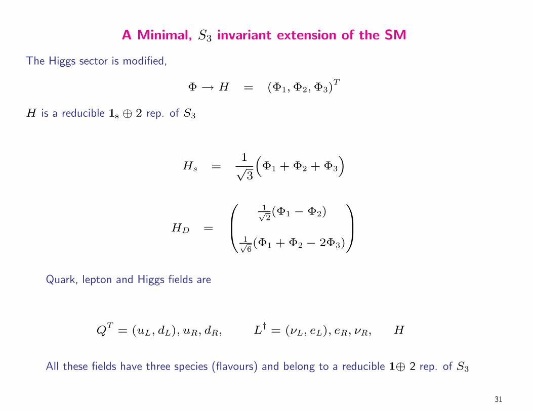
A Minimal, S3 invariant extension of the SM

The Higgs sector is modified,

Φ→ H = (Φ1,Φ2,Φ3)T

H is a reducible 1s ⊕ 2 rep. of S3

Hs =1√3

“

Φ1 + Φ2 + Φ3

”

HD =

0

B

@

1√2(Φ1 − Φ2)

1√6(Φ1 + Φ2 − 2Φ3)

1

C

A

Quark, lepton and Higgs fields are

QT = (uL, dL), uR, dR, L† = (νL, eL), eR, νR, H

All these fields have three species (flavours) and belong to a reducible 1⊕ 2 rep. of S3

31

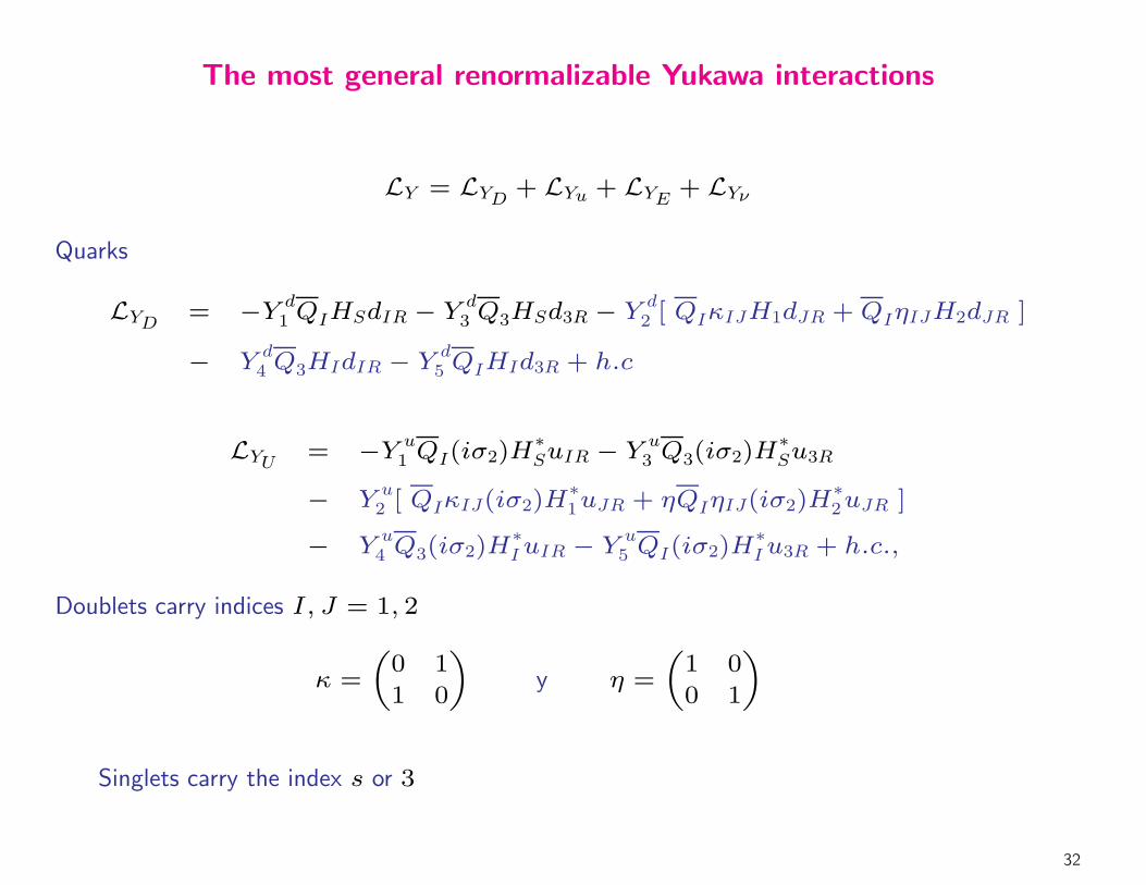
The most general renormalizable Yukawa interactions

LY = LYD + LYu + LYE + LYν

Quarks

LYD = −Y d1 QIHSdIR − Y d

3 Q3HSd3R − Y d2 [ QIκIJH1dJR +QIηIJH2dJR ]

− Yd4 Q3HIdIR − Y d

5 QIHId3R + h.c

LYU = −Y u1 QI(iσ2)H

∗SuIR − Y

u3 Q3(iσ2)H

∗Su3R

− Y u2 [ QIκIJ(iσ2)H

∗1uJR + ηQIηIJ(iσ2)H

∗2uJR ]

− Yu4 Q3(iσ2)H

∗IuIR − Y

u5 QI(iσ2)H

∗Iu3R + h.c.,

Doublets carry indices I, J = 1, 2

κ =

„

0 1

1 0

«

y η =

„

1 0

0 1

«

Singlets carry the index s or 3

32

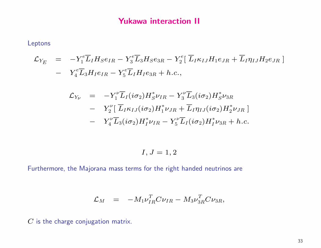
Yukawa interaction II

Leptons

LYE = −Y e1 LIHSeIR − Y e

3 L3HSe3R − Y e2 [ LIκIJH1eJR + LIηIJH2eJR ]

− Ye4 L3HIeIR − Y e

5 LIHIe3R + h.c.,

LYν = −Y ν1 LI(iσ2)H

∗SνIR − Y

ν3 L3(iσ2)H

∗Sν3R

− Yν2 [ LIκIJ(iσ2)H

∗1νJR + LIηIJ(iσ2)H

∗2νJR ]

− Y ν4 L3(iσ2)H

∗IνIR − Y

ν5 LI(iσ2)H

∗Iν3R + h.c.

I, J = 1, 2

Furthermore, the Majorana mass terms for the right handed neutrinos are

LM = −M1νTIRCνIR −M3ν

T3RCν3R,

C is the charge conjugation matrix.

33

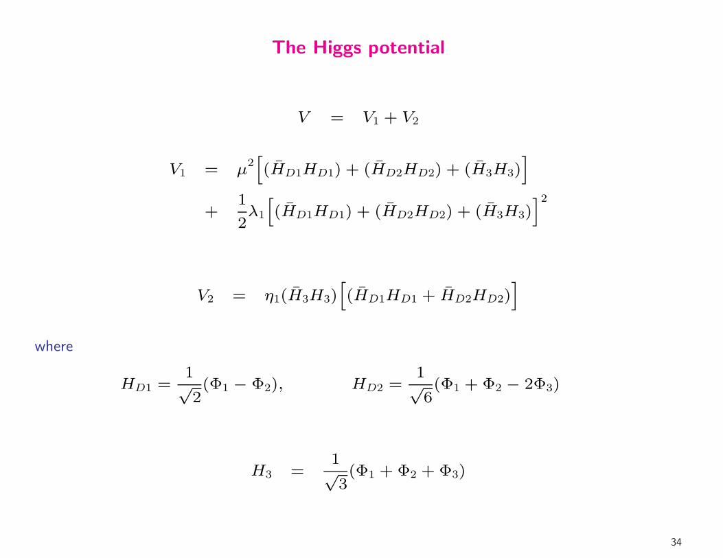
The Higgs potential

V = V1 + V2

V1 = µ2h

(HD1HD1) + (HD2HD2) + (H3H3)i

+1

2λ1

h

(HD1HD1) + (HD2HD2) + (H3H3)i2

V2 = η1(H3H3)h

(HD1HD1 + HD2HD2)i

where

HD1 =1√2(Φ1 − Φ2), HD2 =

1√6(Φ1 + Φ2 − 2Φ3)

H3 =1√

3(Φ1 + Φ2 + Φ3)

34

Mass matrices

We will assume that

< HD1 > = < HD2 > 6= 0 and < H3 > 6= 0

and

< H3 >2 + < HD1 >

2 + < HD2 >2 ≈

“246

2GeV

”2

Then, the Yukawa interactions yield mass matrices of the general form

M =

0

@

µ1 + µ2 µ2 µ5

µ2 µ1 − µ2 µ5

µ4 µ4 µ3

1

A

The Majorana masses for νL are obtained from the see-saw mechanism

Mν = MνDM−1

(MνD)T

with M = diag(M1,M1,M3)

35

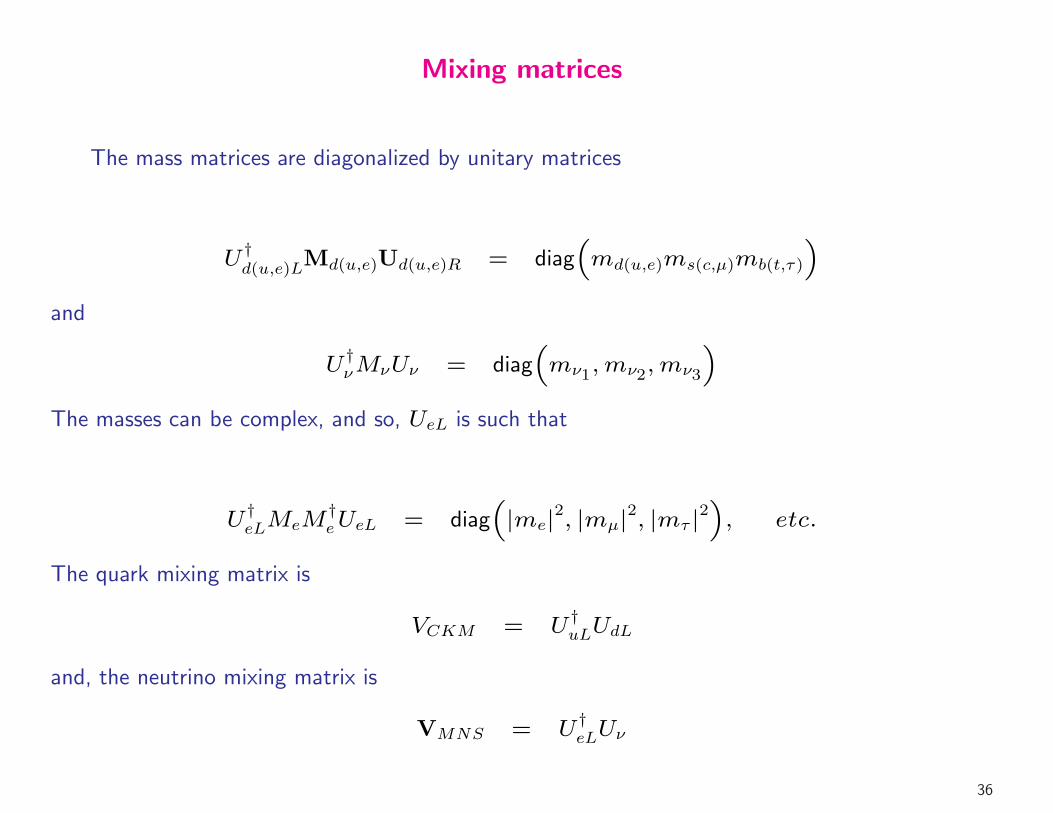
Mixing matrices

The mass matrices are diagonalized by unitary matrices

U†d(u,e)L

Md(u,e)Ud(u,e)R = diag“

md(u,e)ms(c,µ)mb(t,τ)

”

and

U†νMνUν = diag“

mν1,mν2

,mν3

”

The masses can be complex, and so, UeL is such that

U†eLMeM†eUeL = diag

“

|me|2, |mµ|2, |mτ |2”

, etc.

The quark mixing matrix is

VCKM = U†uLUdL

and, the neutrino mixing matrix is

VMNS = U†eLUν

36

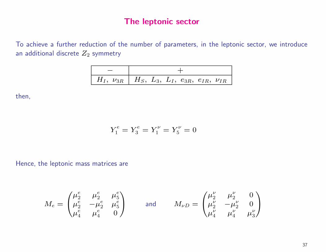
The leptonic sector

To achieve a further reduction of the number of parameters, in the leptonic sector, we introduce

an additional discrete Z2 symmetry

− +

HI, ν3R HS, L3, LI, e3R, eIR, νIR

then,

Ye1 = Y

e3 = Y

ν1 = Y

ν5 = 0

Hence, the leptonic mass matrices are

Me =

0

@

µe2 µe2 µe5µe2 −µe2 µe5µe4 µe4 0

1

A and MνD =

0

@

µν2 µν2 0

µν2 −µν2 0

µν4 µν4 µν3

1

A

37

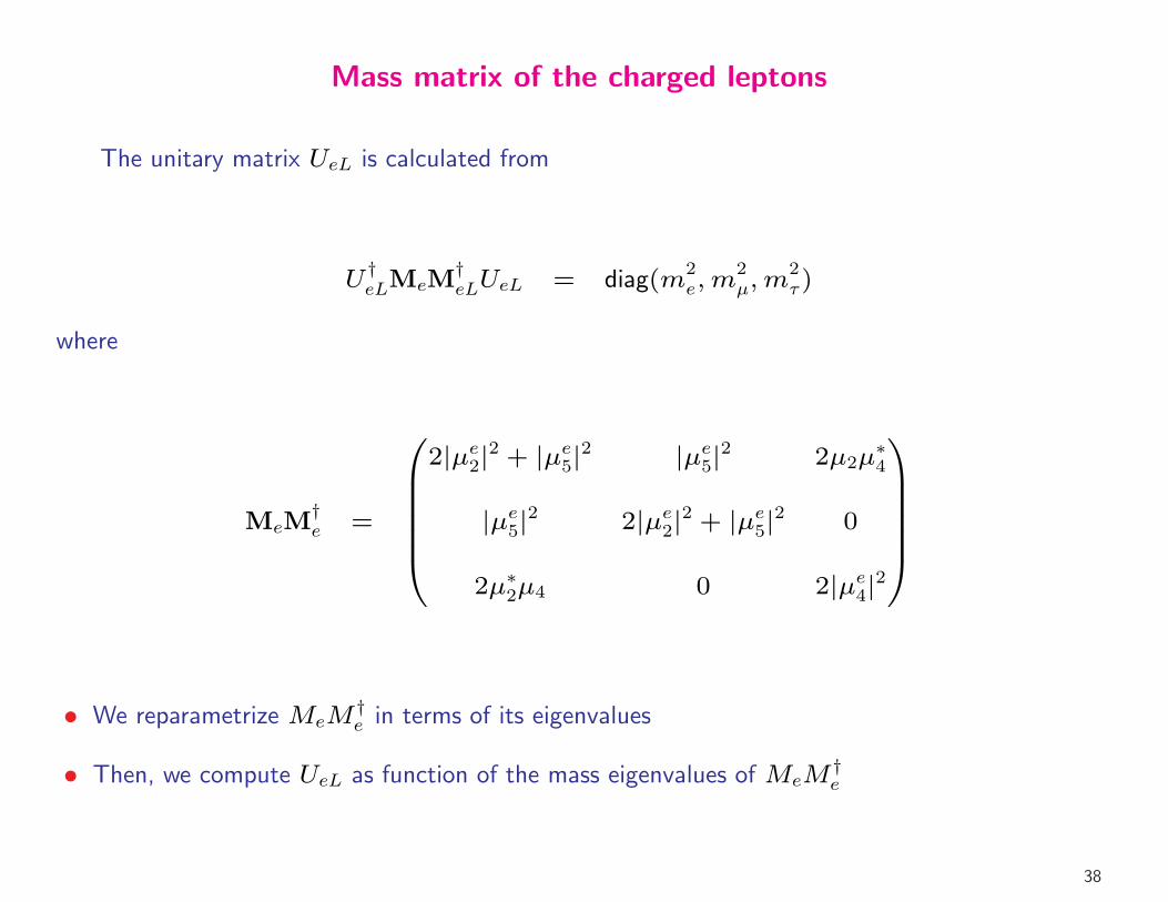
Mass matrix of the charged leptons

The unitary matrix UeL is calculated from

U†eLMeM

†eLUeL = diag(m

2e,m

2µ,m

2τ)

where

MeM†e =

0

B

B

B

B

B

@

2|µe2|2 + |µe5|2 |µe5|2 2µ2µ∗4

|µe5|2 2|µe2|2 + |µe5|2 0

2µ∗2µ4 0 2|µe4|2

1

C

C

C

C

C

A

• We reparametrize MeM†e in terms of its eigenvalues

• Then, we compute UeL as function of the mass eigenvalues of MeM†e

38

Reparametrization of the mass matrix I

From the invariants of MeM†e we obtain

Tr(MeM†e) = m

2e +m

2µ +m

2τ =

m2τ

h

4|µ2|2 + 2“

|µ4|2 + |µ5|2”i

,

χ(MeM†e) = m

2τ(m

2e +m

2µ) +m

2em

2µ =

4m4τ

h

|µ2|4 + |µ2|2“

|µ4|2 + |µ5|2”

+ |µ4|2|µ5|2i

,

and

det(MeM†e) = m

2em

2µm

2τ = 4m

6τ |µ2|2|µ4|2|µ5|2

39

Reparametrization of the Mass Matrix II

Solving for the parameters |µ2|2, |µ4|2, and |µ5|2, in terms of mµ/mτ and me/mτ we get,

|µ2|2 =m2µ

21+x4

1+x2+ β (1)

|µ4,5|2 = 14

“

1− m2µ

(1−x2)2

1+x2− 4β

”

∓14

v

u

u

u

u

t

“

1− m2µ

(1−x2)2

1+x2

”2

− 8m2e1+x2

1+x4+ 8β

0

B

@1− m2

µ(1−x2)2

1+x2+ x2

1+2β(1+x2)

m2µ(1+x4)

(1+x2)2

(1+x4)2

1

C

A+ 16β2

(2)

and

x = me/mµ, β ≈ 1

2

m2em

2µ

m4τ

40

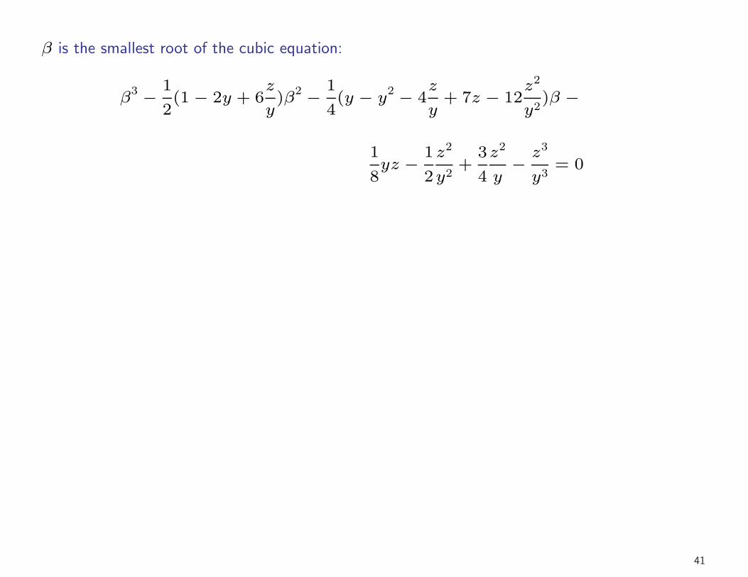
β is the smallest root of the cubic equation:

β3 − 1

2(1− 2y + 6

z

y)β

2 − 1

4(y − y2 − 4

z

y+ 7z − 12

z2

y2)β −

1

8yz − 1

2

z2

y2+

3

4

z2

y− z3

y3= 0

41

The Mass Matrix of the charged leptons as function of its eigenvalues

The mass matrix of the charged leptons is

Me ≈ mτ

0

B

B

B

B

B

B

B

B

B

B

B

@

1√2

mµ√1+x2

1√2

mµ√1+x2

1√2

r

1+x2−m2µ

1+x2

1√2

mµ√1+x2

− 1√2

mµ√1+x2

1√2

r

1+x2−m2µ

1+x2

me(1+x2)

q

1+x2−m2µ

eiδeme(1+x

2)q

1+x2−m2µ

eiδe 0

1

C

C

C

C

C

C

C

C

C

C

C

A

. (3)

This expression is accurate to order 10−9 in units of the τ mass

There are no free parameters in Me other than the Dirac Phase δ!!

42

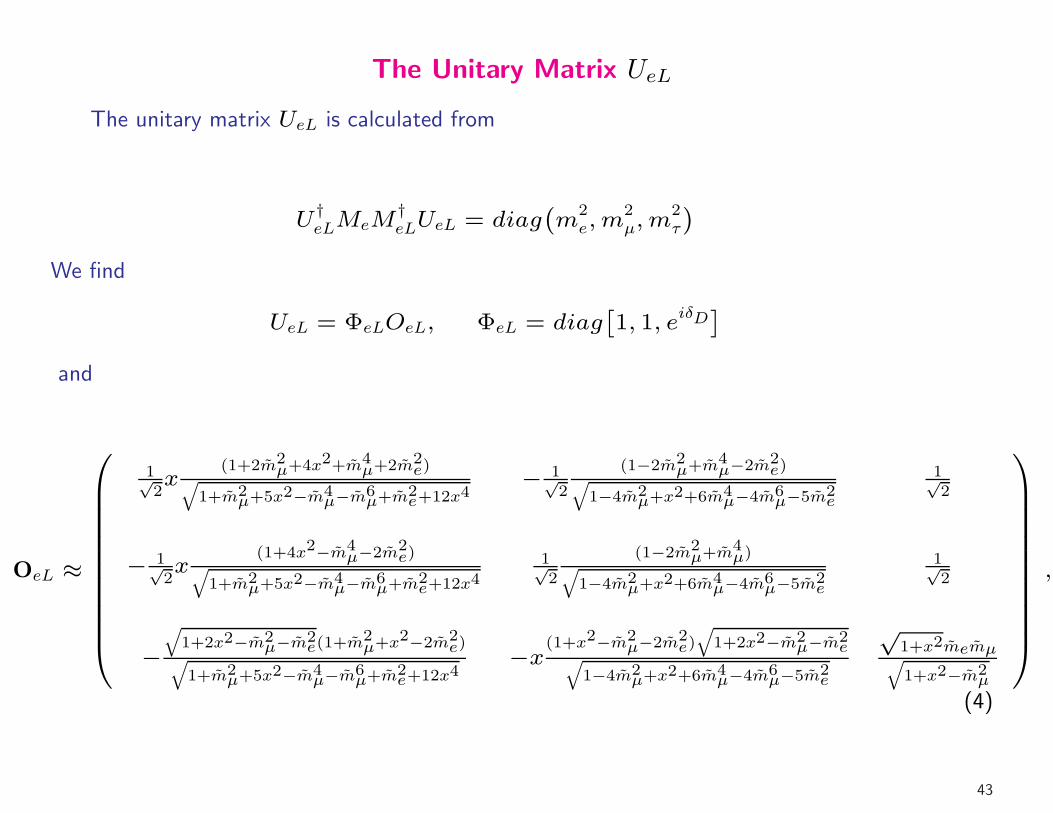
The Unitary Matrix UeL

The unitary matrix UeL is calculated from

U†eLMeM

†eLUeL = diag

`

m2e,m

2µ,m

2τ

´

We find

UeL = ΦeLOeL, ΦeL = diagˆ

1, 1, eiδD˜

and

OeL ≈

0

B

B

B

B

B

B

B

B

B

B

B

@

1√2x

(1+2m2µ+4x2+m4

µ+2m2e)

q

1+m2µ+5x2−m4

µ−m6µ+m2

e+12x4− 1√

2

(1−2m2µ+m4

µ−2m2e)

q

1−4m2µ+x2+6m4

µ−4m6µ−5m2

e

1√2

− 1√2x

(1+4x2−m4µ−2m2

e)q

1+m2µ+5x2−m4

µ−m6µ+m2

e+12x4

1√2

(1−2m2µ+m4

µ)q

1−4m2µ+x2+6m4

µ−4m6µ−5m2

e

1√2

−q

1+2x2−m2µ−m2

e(1+m2µ+x2−2m2

e)q

1+m2µ+5x2−m4

µ−m6µ+m2

e+12x4−x(1+x2−m2

µ−2m2e)q

1+2x2−m2µ−m2

eq

1−4m2µ+x2+6m4

µ−4m6µ−5m2

e

√1+x2memµq

1+x2−m2µ

1

C

C

C

C

C

C

C

C

C

C

C

A

,

(4)

43

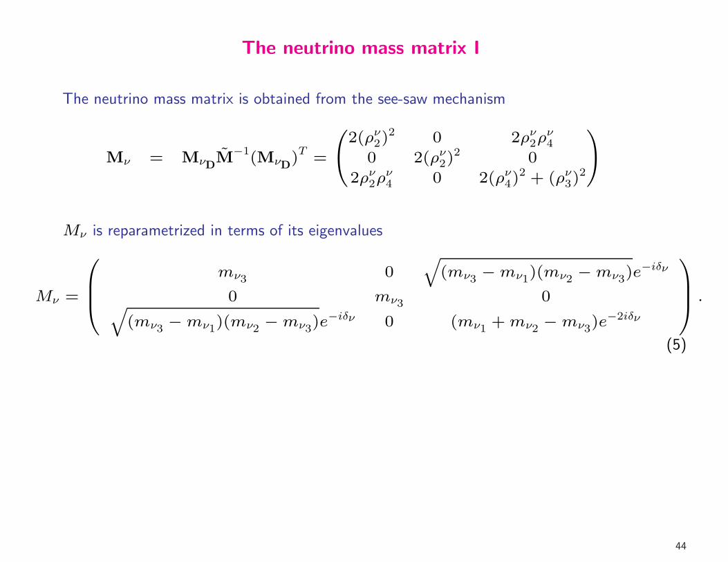
The neutrino mass matrix I

The neutrino mass matrix is obtained from the see-saw mechanism

Mν = MνDM−1(MνD

)T =

0

@

2(ρν2)2 0 2ρν2ρ

ν4

0 2(ρν2)2 0

2ρν2ρν4 0 2(ρν4)

2 + (ρν3)2

1

A

Mν is reparametrized in terms of its eigenvalues

Mν =

0

B

B

@

mν30

q

(mν3−mν1

)(mν2−mν3

)e−iδν

0 mν3 0q

(mν3−mν1

)(mν2−mν3

)e−iδν 0 (mν1+mν2

−mν3)e−2iδν

1

C

C

A

.

(5)

44

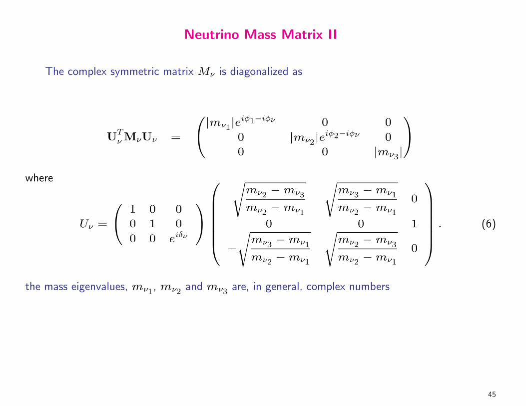
Neutrino Mass Matrix II

The complex symmetric matrix Mν is diagonalized as

UTνMνUν =

0

@

|mν1|eiφ1−iφν 0 0

0 |mν2|eiφ2−iφν 0

0 0 |mν3|

1

A

where

Uν =

0

@

1 0 0

0 1 0

0 0 eiδν

1

A

0

B

B

B

B

B

B

@

s

mν2−mν3

mν2−mν1

s

mν3−mν1

mν2−mν1

0

0 0 1

−s

mν3−mν1

mν2 −mν1

s

mν2−mν3

mν2 −mν1

0

1

C

C

C

C

C

C

A

. (6)

the mass eigenvalues, mν1, mν2 and mν3 are, in general, complex numbers

45

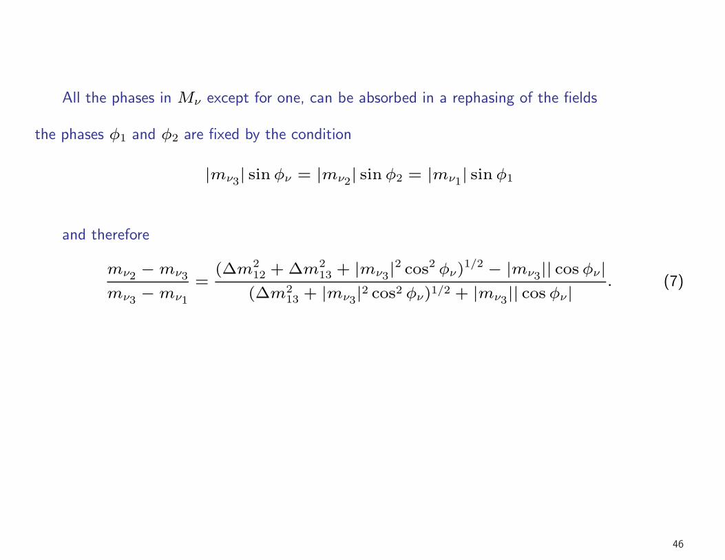
All the phases in Mν except for one, can be absorbed in a rephasing of the fields

the phases φ1 and φ2 are fixed by the condition

|mν3| sinφν = |mν2

| sinφ2 = |mν1| sinφ1

and therefore

mν2−mν3

mν3−mν1

=(∆m2

12 + ∆m213 + |mν3

|2 cos2 φν)1/2 − |mν3

|| cosφν|(∆m2

13 + |mν3|2 cos2 φν)1/2 + |mν3

|| cosφν|. (7)

46

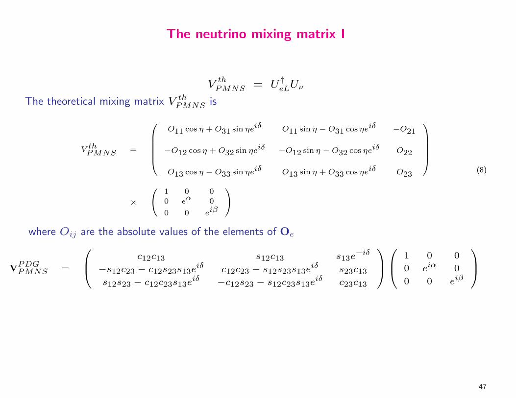
The neutrino mixing matrix I

V thPMNS = U†eLUν

The theoretical mixing matrix V thPMNS is

V thPMNS =

0

B

B

B

B

B

@

O11 cos η +O31 sin ηeiδ O11 sin η − O31 cos ηeiδ −O21

−O12 cos η + O32 sin ηeiδ −O12 sin η − O32 cos ηeiδ O22

O13 cos η − O33 sin ηeiδ O13 sin η +O33 cos ηeiδ O23

1

C

C

C

C

C

A

×

0

@

1 0 00 eα 0

0 0 eiβ

1

A

(8)

where Oij are the absolute values of the elements of Oe

VPDGPMNS =

0

B

@

c12c13 s12c13 s13e−iδ

−s12c23 − c12s23s13eiδ c12c23 − s12s23s13eiδ s23c13s12s23 − c12c23s13eiδ −c12s23 − s12c23s13eiδ c23c13

1

C

A

0

B

@

1 0 0

0 eiα 0

0 0 eiβ

1

C

A

47

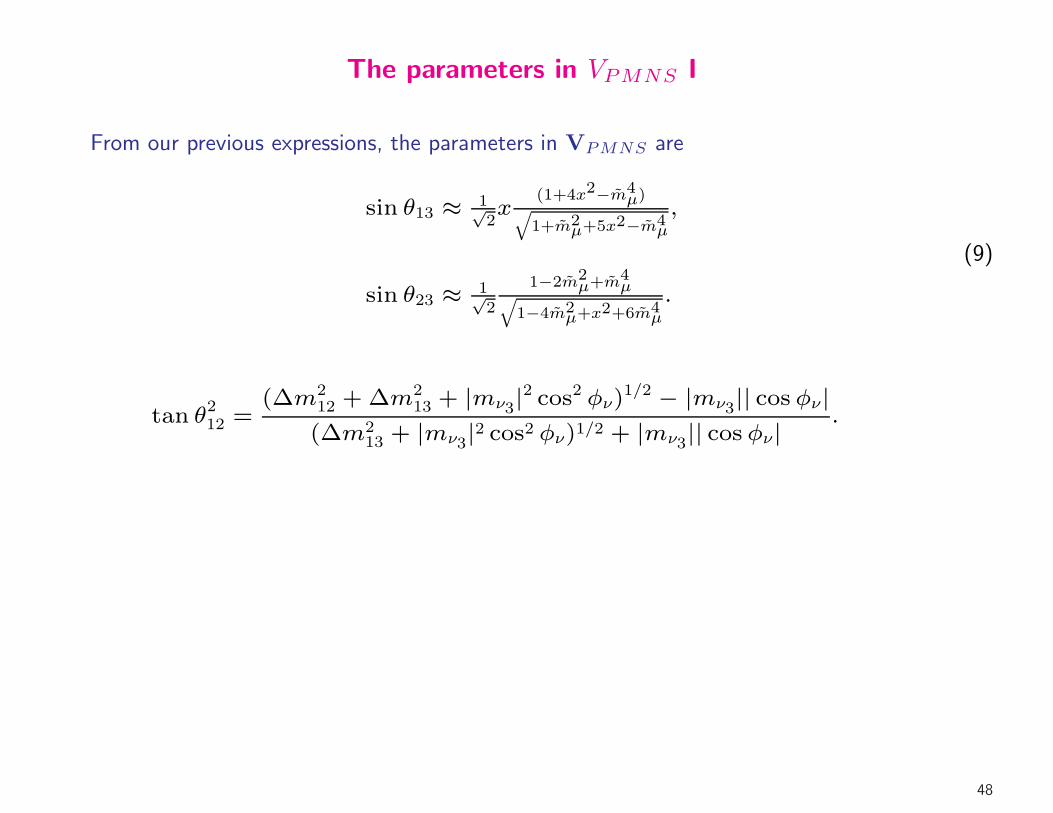
The parameters in VPMNS I

From our previous expressions, the parameters in VPMNS are

sin θ13 ≈ 1√2x

(1+4x2−m4µ)

q

1+m2µ+5x2−m4

µ

,

sin θ23 ≈ 1√2

1−2m2µ+m4

µq

1−4m2µ+x2+6m4

µ

.

(9)

tan θ212 =

(∆m212 + ∆m2

13 + |mν3|2 cos2 φν)

1/2 − |mν3|| cosφν|

(∆m213 + |mν3

|2 cos2 φν)1/2 + |mν3|| cosφν|

.

48

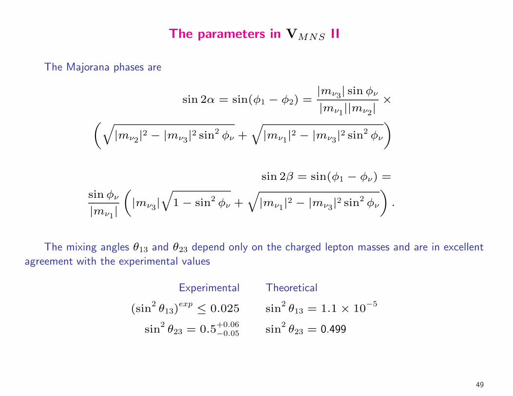
The parameters in VMNS II

The Majorana phases are

sin 2α = sin(φ1 − φ2) =|mν3| sinφν

|mν1||mν2|×

„

q

|mν2|2 − |mν3

|2 sin2 φν +q

|mν1|2 − |mν3

|2 sin2 φν

«

sin 2β = sin(φ1 − φν) =

sinφν

|mν1|

„

|mν3|q

1− sin2 φν +q

|mν1|2 − |mν3

|2 sin2 φν

«

.

The mixing angles θ13 and θ23 depend only on the charged lepton masses and are in excellent

agreement with the experimental values

Experimental Theoretical

(sin2θ13)

exp ≤ 0.025 sin2θ13 = 1.1× 10

−5

sin2θ23 = 0.5

+0.06−0.05 sin

2θ23 = 0.499

49

The neutrino mass spectrum I

In the present model, the experimental restriction

|∆m221| < |∆m

223|

implies an inverted neutrino mass spectrum mν3< mν1

,mν2

From our previous expressions

|mν3| =

q

∆m213

2 cosφν tan θ12

1− tan4 θ12 + r2

p

1 + tan2 θ12

p

1 + tan2 θ12 + r2,

where r = ∆m221/∆m

223.

The mass |mν3| assumes its minimal value when sinφν = 0,

|mν3| ≈ 1

2

q

∆m213

tan θ12

(1− tan2 θ12)

50

Neutrino mass spectrum II

• We wrote the neutrino mass differences, mνi−mνj

, in terms of the differences of the squared

masses ∆2ij = m2

νi−m2

νjand one of the neutrino masses, say mν3

.

• The mass mν2was taken as a free parameter in the fitting of our formula for tan θ12 to the

experimental value

• with

∆m213 = 2.6× 10

−3eV

2∆m

221 = 7.9× 10

−5eV

2

and

tan θ12 = 0.667

we get

|mν3| ≈ 0.022eV =⇒ |mν2

| ≈ 0.056eV and |mν1| ≈ 0.055eV

51

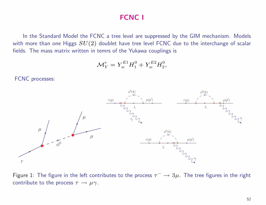
FCNC I

In the Standard Model the FCNC a tree level are suppressed by the GIM mechanism. Models

with more than one Higgs SU(2) doublet have tree level FCNC due to the interchange of scalar

fields. The mass matrix written in temrs of the Yukawa couplings is

MeY = Y

E1w H

01 + Y

E2w H

02 ,

FCNC processes:

τ

φ0

µ

µ

µ

τ(p)

τ(p)

τ(p)µ(p′) µ(p′)

µ(p′)

φ0(k)

li li

φ0(k)

φ0(k)

li

γ

γ

γ

Figure 1: The figure in the left contributes to the process τ− → 3µ. The tree figures in the right

contribute to the process τ → µγ.

52

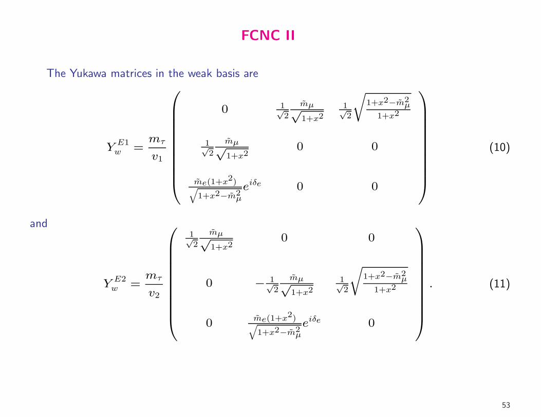
FCNC II

The Yukawa matrices in the weak basis are

YE1w =

mτ

v1

0

B

B

B

B

B

B

B

B

B

B

@

0 1√2

mµ√1+x2

1√2

r

1+x2−m2µ

1+x2

1√2

mµ√1+x2

0 0

me(1+x2)

q

1+x2−m2µ

eiδe 0 0

1

C

C

C

C

C

C

C

C

C

C

A

(10)

and

Y E2w =

mτ

v2

0

B

B

B

B

B

B

B

B

B

B

@

1√2

mµ√1+x2

0 0

0 − 1√2

mµ√1+x2

1√2

r

1+x2−m2µ

1+x2

0 me(1+x2)

q

1+x2−m2µ

eiδe 0

1

C

C

C

C

C

C

C

C

C

C

A

. (11)

53

FCNC III

The Yukawa matrices in the mass basis defined by

Y EIm = U†eLY

EIw UeR

YE1m ≈ mτ

v1

0

B

B

B

B

B

@

2me −12me

12x

−mµ12mµ −1

2

12mµx

2 −12mµ

12

1

C

C

C

C

C

A

m

,

and

Y E2m ≈ mτ

v2

0

B

B

B

B

B

@

−me12me −1

2x

mµ12mµ

12

−12mµx

2 12mµ

12

1

C

C

C

C

C

A

m

,

54

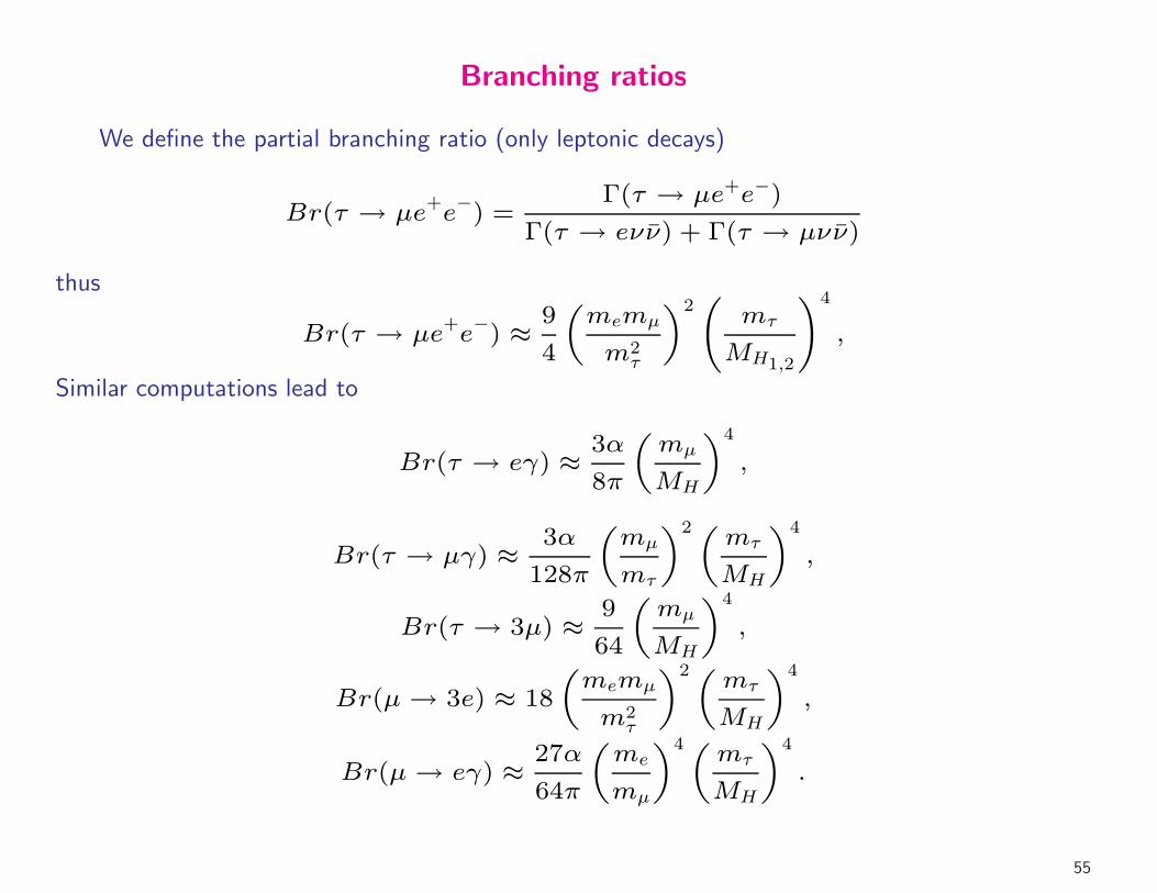
Branching ratios

We define the partial branching ratio (only leptonic decays)

Br(τ → µe+e−) =Γ(τ → µe+e−)

Γ(τ → eνν) + Γ(τ → µνν)

thus

Br(τ → µe+e−) ≈ 9

4

„

memµ

m2τ

«2

mτ

MH1,2

!4

,

Similar computations lead to

Br(τ → eγ) ≈ 3α

8π

„

mµ

MH

«4

,

Br(τ → µγ) ≈ 3α

128π

„

mµ

mτ

«2„mτ

MH

«4

,

Br(τ → 3µ) ≈ 9

64

„

mµ

MH

«4

,

Br(µ→ 3e) ≈ 18

„

memµ

m2τ

«2„mτ

MH

«4

,

Br(µ→ eγ) ≈ 27α

64π

„

me

mµ

«4„mτ

MH

«4

.

55

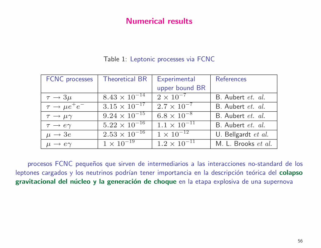
Numerical results

Table 1: Leptonic processes via FCNC

FCNC processes Theoretical BR Experimental References

upper bound BR

τ → 3µ 8.43× 10−14 2× 10−7 B. Aubert et. al.

τ → µe+e− 3.15× 10−17 2.7× 10−7 B. Aubert et. al.

τ → µγ 9.24× 10−15 6.8× 10−8 B. Aubert et. al.

τ → eγ 5.22× 10−16 1.1× 10−11 B. Aubert et. al.

µ→ 3e 2.53× 10−16 1× 10−12 U. Bellgardt et al.

µ→ eγ 1× 10−19 1.2× 10−11 M. L. Brooks et al.

procesos FCNC pequenos que sirven de intermediarios a las interacciones no-standard de los

leptones cargados y los neutrinos podrıan tener importancia en la descripcion teorica del colapso

gravitacional del nucleo y la generacion de choque en la etapa explosiva de una supernova

56

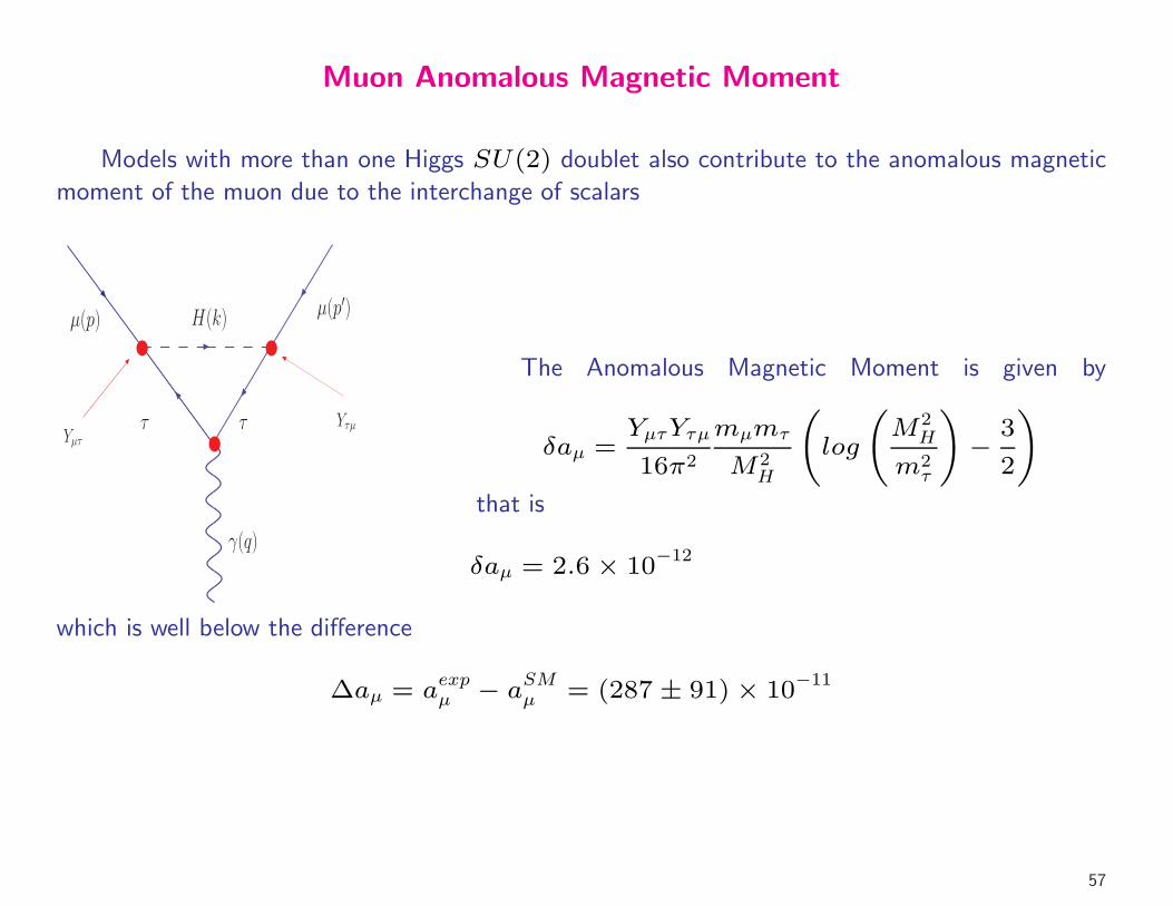
Muon Anomalous Magnetic Moment

Models with more than one Higgs SU(2) doublet also contribute to the anomalous magnetic

moment of the muon due to the interchange of scalars

µ(p′)H(k)µ(p)

γ(q)

ττYµτ

Yτµ

The Anomalous Magnetic Moment is given by

δaµ =YµτYτµ

16π2

mµmτ

M2H

log

M2H

m2τ

!

− 3

2

!

that is

δaµ = 2.6× 10−12

which is well below the difference

∆aµ = aexpµ − aSMµ = (287± 91)× 10−11

57

Conclusions I

• By introducing three SU(2)L Higgs doublet fields in the theory, we extended the concept of

flavour and generations to the Higss sector and formulated a minimal S3−invariant Extension

of the Standard Model

• A definite structure of the Yukawa couplings is obtained which permits the calculation of mass

and mixing matrices for quarks and leptons in a unified way

• A further reduction of free parameters is achieved in the leptonic sector by introducing a Z2

symmetry.

• The three charged lepton masses, three Majorana masses of the left-handed neutrinos and

the three mixing angles and the 2 Majorana phases are computed in terms of only seven free

parameters, in agreement with all the experimental observations at this time

• The magnitudes of the three mixing angles, θ12, θ23 , and θ13, are determined by an interplay

of the S3 × Z2 symmetry, the see saw mechanism and the lepton mass hierachy

58

Conclusions II

• The mixing angles θ23 and θ13 are insensitive to the values of the neutrino masses

• The solar mixing angle fixes the scale and origen of the mass spectrum

• The neutrino mass spectrum has an inverted mass hierarchy with the values

|mν2| ≈ 0.056eV, |mν1

| ≈ 0.055eV |mν3| ≈ 0.022eV,

• Numerical values for FCNC below experimental constraints

• FCNC processes considered are strongly suppressed by powers of the small mass ratios me/mτ

and mµ/mτ , and by the ratio“

mτ/MH1,2

”4

• Could be important in astrophysical processes

59