FISH AND TROPHIC CONNECTIVITY ACROSS CORAL REEF

AND MANGROVE HABITATS OF NORTH EASTERN

LANGKAWI ISLAND, PENINSULAR MALAYSIA

LAU CHAI MING

DISSERTATION SUBMITTED IN FULFILMENT OF

THE REQUIREMENTS FOR THE DEGREE OF

MASTER OF SCIENCE

INSTITUTE OF BIOLOGICAL SCIENCES

FACULTY OF SCIENCE

UNIVERSITY OF MALAYA

KUALA LUMPUR

2014

UNIVERSITI MALAYA

ORIGINAL LITERARY WORK DECLARATION

Name of Candidate: LAU CHAI MING

I/C/Passport No: 850409-05-5121

Regisration/Matric No.: SGR090054

Name of Degree: MASTER OF SCIENCE

Title of Project Paper/Research Report/Dissertation/Thesis (“this Work”):

“FISH AND TROPHIC CONNECTIVITY ACROSS CORAL REEF AND MANGROVE

HABITATS OF NORTH EASTERN LANGKAWI ISLAND, PENINSULAR MALAYSIA”

Field of Study: MARINE ECOLOGY & BIODIVERSITY

I do solemnly and sincerely declare that:

(1) I am the sole author/writer of this Work, (2) This Work is original,

(3) Any use of any work in which copyright exists was done by way of fair dealing and for

permitted purposes and any excerpt or extract from, or reference to or reproduction of any

copyright work has been disclosed expressly and sufficiently and the title of the Work and its authorship have been acknowledged in this Work,

(4) I do not have any actual knowledge nor do I ought reasonably to know that the making of

this work constitutes an infringement of any copyright work, (5) I hereby assign all and every rights in the copyright to this Work to the University of Malaya

(“UM”), who henceforth shall be owner of the copyright in this Work and that any

reproduction or use in any form or by any means whatsoever is prohibited without the written consent of UM having been first had and obtained,

(6) I am fully aware that if in the course of making this Work I have infringed any copyright

whether intentionally or otherwise, I may be subject to legal action or any other action as

may be determined by UM.

(Candidate Signature) Date:

Subscribed and solemnly declared before,

Witness’s Signature Date:

Name PROFESSOR DR CHONG VING CHING

Designation

iii

ABSTRACT

The presence of disparate biotopes of coral reefs and mangroves in one general area is

unique. These biotopes may form ecologically connected ecosystems when occurring in

close proximity such as in tropical Langkawi Island, Malaysia. Connected marine

biotopes can provide various ecological services to fish community such as nursery,

feeding habitats and shelter. As such, this study aims to test two hypotheses regarding

Langkawi’s coral reefs and mangroves 1) the biotopes are ecologically connected via

habitat utilization by the fish fauna and 2) the biotopes are ecologically connected via

trophic energy pathways. Gill nets and fish pots were deployed to determine common

overlapping fish species in both biotopes. Samples of primary producers, sediment and

consumers were subjected to dual stable isotope analysis and stomach content analysis

in the case of fishes. Coral community and habitat complexity as proxies for refuge

cover were determined based on r-K-S adaptive strategists and coral morphology

diversity respectively. The present study discovered a relatively high number of

common species, 31 out of a total of 149 fish species, suggested there was movement of

fishes between habitats. Despite the turbid water, the coral cover was considerably high,

47.21% with low mortality and dominated by stress-tolerators. The habitat complexity

was also relatively high with 2.06 index of morphological diversity indicated a fairly

good refuge area. Stomach content analysis of fish revealed benthic invertebrates and

small nekton as the main food items. Stable isotope analysis showed that the δ13

C

values of zooplankton (-21.66 ± 0.72 ‰ SE) were closer to phytoplankton (-21.64 ±

0.79 ‰ SE). The fishes even as far as the upstream mangrove had relatively enriched

δ13

C values (-8.88 to -22.37 ‰) close to the values of coral zooxanthellae (-15.39 ± 0.33

‰ SE) and phytoplankton, but distinctly distant from mangrove-derived source (-28.83

± 0.38 ‰ SE). A Bayesian mixing model of stable isotopic analysis in R (SIAR)

iv

depicted coral zooxanthellae as the major carbon contributor to fish nutrition in the

coral reefs (90.0%) and mangrove (63.7%). Since phytoplankton contributed 32.0% in

the mangrove estuary, mangrove carbon was relatively unimportant to the food web

even in the mangrove estuary itself. Under the turbid water condition, mucus

productions are expected by corals. It is hypothesized that coral mucus and zooplankton

are the vehicles of energy transfer from coral zooxanthellae to consumers in the

mangrove habitat. The present study suggests that fish movements and outwelling of

extruded mucus and zooplankton connect coral reef to mangrove.

v

ABSTRAK

Kewujudan habitat yang berbeza seperti terumbu karang dan bakau di satu kawasan

umum adalah unik. Kedua habitat ini boleh membentuk ekosistem yang terkait secara

ekologi apabila wujud berhampiran seperti yang terdapat di Pulau Langkawi, Malaysia.

Habitat marin yang terkait boleh memberi pelbagai khidmat ekologi kepada komuniti

ikan seperti tapak semaian, habitat makanan dan juga tempat berlindung. Justeru itu,

kajian ini adalah untuk menguji dua hipotesis tentang terumbu karang dan bakau di

Langkawi iaitu 1) kedua-dua biotop adalah terkait secara ekologi melalui penggunaan

habitat oleh fauna ikan 2) kedua-dua biotop adalah terkait secara ekologi melalui

pengaliran tenaga trofik. Pukat hanyut dan bubu dipasang untuk menentukan spesis

ikan yang sama di kedua habitat. Sampel bagi pengeluar utama, sedimen dan pengguna

telah dianalisis dengan menggunakan kaedah dwi isotop stabil dan kandungan perut

bagi ikan. Komuniti karang dan kekompleksan habitat sebagai proksi perlindungan telah

ditentukan melalui strategi adaptasi r-K-S dan kepelbagaian morfologi karang. Kajian

ini mendapati bilangan spesies ikan yang sama (31 spesies) bagi kedua habitat adalah

agak tinggi daripada jumlah 149 spesis ikan disampel. Ini memberikan bukti bahawa

terdapat pergerakan ikan di antara kedua habitat yang dikaji. Walaupun keadaan air laut

keruh, liputan karang adalah agak tinggi, 47.21% dengan kadar kematian yang rendah

dan didominasi karang yang bertoleransi tinggi terhadap tekanan alam sekitar.

Kekompleksan habitat juga agak tinggi dengan indeks kepelbagaian morfologi sebanyak

2.06. Ini menunjukkan bahawa ianya suatu kawasan perlindungan yang agak baik.

Analisis kandungan perut ikan menunjukkan bahawa makanan utamanya adalah ikan

kecil dan invertebrata bentik. Analisis isotop stabil menunjukkan bahawa nilai δ13

C

zooplankton (-21.66 ± 0.72 ‰ SE) adalah hampir sama kepada nilai fitoplankton (-

21.64 ± 0.79 ‰ SE). Ikan-ikan termasuklah yang dijumpai dalam bakau di hulu sungai

vi

mempunyai nilai δ13

C (-8.88 to -22.37 ‰) yang hampir sama kepada nilai zooxantela

karang (-15.39 ± 0.33 ‰ SE) dan fitoplankton tetapi jauh daripada nilai sumber bakau (-

28.83 ± 0.38 ‰ SE). Model campuran Bayesian analisis isotop stabil dalam R (SIAR)

menggambarkan zooxantela karang sebagai penyumbang utama karbon kepada

pemakanan ikan dalam habitat terumbu karang (90.0%) dan bakau (63.7%).

Memandangkan fitoplankton menyumbangkan 32.0% karbon dalam bakau, karbon

bakau adalah kurang penting kepada jaringan makanan dalam kawasan bakau. Dalam

keadaan air yang keruh, penghasilan mukus karang adalah dijangkakan tinggi. Oleh itu,

dihipotesiskan bahawa mukus karang dan zooplankton adalah pembawa bagi pertukaran

tenaga kepada pengguna dalam habitat bakau. Daripada hasil kajian adalah dicadangkan

bahawa pergerakan ikan dan pengaliran keluar mukus karang dan zooplankton

memperkaitkan terumbu karang kepada bakau.

vii

ACKNOWLEDGEMENTS

First and foremost, I would like to deeply thank my supervisor, Professor Dr. Chong

Ving Ching for all his time and effort in giving wise advice, esteemed guidance, highly

spirited motivation and encouragement along with invaluable mentoring. Your

kindness, care and concern on our welfare have been wonderful and it is an honour to be

a student under your supervision.

Next, I would like to express my gratitude to my co-supervisor, who is also a mentor to

me, Mr. Affendi Yang Amri for all his patient guidance, advice, ideas and invaluable

help particularly in works related to corals. Thanks to you, I am able to keep my

interests in coral related research.

I wish to thank the University of Malaya for the Skim Biasiswazah Universiti Malaya

(SBUM), the use of facilities and also the University of Malaya Research Grant

(UMRG) Project No: RG012-09SUS which enabled me to undertake and complete this

project.

I am entirely indebted to the fisherman, Hasbi who tirelessly helped in samples

collection even during unfriendly weather. My special thanks also go out to East Marine

Dive Centre and its crews especially Ms. Jenni, who provided diving gears and tanks at

discounted rates.

My gratitude also goes out to my field buddy, Adam who has always been helpful and a

great companion in fieldwork. Thanks for all the fun and joy during our sampling and

exploration trips. Thank you also to my wonderful bunch of B201 labmates, Li Lee,

Moh, Ai Lin, Jamizan (Dagoo), Raven, Tueanta, Jin Yung, Ng, Raymond, Loo and

Teoh for keeping the fun in the lab.

viii

I would also like to express my utmost appreciation to Faedz, Dr. Yuen, Dr. Louisa, Dr.

Loh, Dr. Sase, Kee, for all their ideas and help along the way in completing the work

and to Dr. Khang for the statistical advice. To Cecilia, Lutfi, Kojet, Marzuki, Mimi,

Azmut and Jamat, I just want to thank you for your help. Thank you to Mark and Anke

as well as Amy for your comments on the English in the thesis. I would also like to

shout out my thanks to the ISB drivers and Jebri as well as all staffs in the university.

The most instrumental people, my beloved family, Mom and Dad, Eddie, Edwina,

Eddora, Kak Arnida whom have been very supportive and kept me going even during

difficult times while working on the study, I deeply thank you and love you all!

The pillar of my strength has always been my dearest and most beloved darling Kuan

Ching, who always stood by me with continuous support, trust and love. I will never

forget your sacrifice, patience and you will always remain in my heart. Thank you and

love you deeply!

Last but not least, I wish to thank Lord Buddha for all His teachings that had kept me on

my ground and never giving up in pursuing my passion in the work.

ix

TABLE OF CONTENTS

PAGE

TITLE PAGE .............................................................................................................. i

ORIGINAL LITERARY WORK DECLARATION ................................................ ii

ABSTRACT .............................................................................................................. iii

ABSTRAK .................................................................................................................. v

ACKNOWLEDGEMENTS ..................................................................................... vii

TABLE OF CONTENTS .......................................................................................... ix

LIST OF FIGURES .................................................................................................. xi

LIST OF TABLES .................................................................................................. xiii

LIST OF ABBREVIATIONS .................................................................................. xv

LIST OF APPENDICES ......................................................................................... xvi

CHAPTER ONE

1.0 INTRODUCTION ................................................................................................. 1

1.1 What is connectivity? ............................................................................ 1

1.2 Ecological connectivity of biotopes ....................................................... 1

1.3 Coral reefs .............................................................................................. 2

1.4 Mangroves ............................................................................................. 4

1.5 Physical attributes of seawater and habitat complexity ....................... 5

1.6 Source contribution ................................................................................ 7

1.7 Stomach content and stable isotope analysis ....................................... 10

1.8 Research problems and questions ........................................................ 11

1.9 Significance of study ............................................................................. 13

1.10 Hypotheses and objectives .................................................................... 15

CHAPTER TWO

2.0 METHODOLOGY .............................................................................................. 16

2.1 Study site and habitat zoning ............................................................... 16

2.2 Fieldwork collection and sampling ...................................................... 19

2.2.1 Physical attributes of seawater .................................................. 19

2.2.2 Collection of fish samples ........................................................ 20

2.2.3 Measurements and identification of fish samples ...................... 20

2.2.4 Collection of corals and other samples...................................... 21

2.2.5 Coral community structure ....................................................... 21

2.3 Laboratory work .................................................................................. 23

x

2.3.1 Examination of stomach contents ............................................. 23

2.3.2 Sample preparation for isotopic analysis ................................... 23

2.4 Data analysis ......................................................................................... 25

2.4.1 Physical attributes of seawater and life forms cover .................. 25

2.4.2 Fish species cluster analysis ..................................................... 26

2.4.3 Habitat complexity and mortality index .................................... 26

2.4.4 Stomach content and Stable Isotope Analysis in R (SIAR) ....... 27

CHAPTER THREE

3.0 RESULTS ............................................................................................................ 29

3.1 Seawater physical attributes of biotopes ............................................. 29

3.2 Fish species diversity and similarity .................................................... 32

3.3 Coral community structure and habitat complexity ........................... 43

3.4 Stomach content analysis to determine trophic guilds ........................ 48

3.5 Stable isotopes of producers and consumers ....................................... 48

3.6 Fish nutrition by habitat zones ............................................................ 60

3.7 Source contribution to zooplankton and fish nutrition ....................... 60

CHAPTER FOUR

4.0 DISCUSSIONS .................................................................................................... 63

4.1 Source contribution to fish community ............................................... 63

4.2 Physical attributes of biotopes ............................................................. 66

4.3 Fish species diversity and similarity .................................................... 69

4.4 Habitat complexity ............................................................................... 73

4.5 Synthesis of findings ............................................................................. 77

4.6 Limitations of present study and suggestions for future research ...... 83

CHAPTER FIVE

5.0 CONCLUSION ................................................................................................... 85

REFERENCES ......................................................................................................... 86

xi

LIST OF FIGURES

Fig. 2.1 The study area, north east Langkawi separated into four major study sites, Tg.

Rhu, Kilim, Peluru Strait and Kisap. Sampling stations are shown in the legend above.

Sa, Sb and Sc represent stations whereby seston samples were collected from mangrove

creeks, mangrove estuary and nearshore waters respectively ....................................... 17

Fig. 2.2 Diagrammatic representations of the four habitat zones; coral (Coral), mixed

mangrove-coral (Mg-C), mangrove estuary (Mg) and creeks (Up). The coral zone is

encompassed by only the coral biotope while the Mg and Up zones are flanked by

mangrove forests. Mg-C zone is the mixed habitat of corals that grow on the submerged

limestone massive flanked by mangrove on the upper shore ........................................ 17

Fig. 2.3 Diagrammatic illustration of the connectivity between Coral Reef Biotope

and Mangrove Biotope which encompass their respective zones. Mixed mangrove –

coral zone (Mg-C) is excluded from either biotope because it is a mixed of overlapping

biotopes……............................................................................................................... 19

Fig. 2.4 Food web design based on the feeding guilds assigned to calculate the trophic

shift (∆13

C, ∆15

N). Arrows points from source to consumers with percentages indicating

proportions of diets consumed and trophic shift values stated in brackets (+ 13

C, + 15

N).

These proportional trophic shift values were used to calculate ∆13

C and ∆15

N. Primary

Consumers (Invertebrates) are included in the design because they are at least one

trophic level higher than the primary source ................................................................ 28

Fig. 3.1 Dendogram from complete linkage cluster analysis of fish species in North

East of Langkawi using presence-absence data. Three distinct clusters of (a), (b) and (c)

were able to be established .......................................................................................... 34

Fig. 3.2 Dendogram from complete linkage percent disagreement cluster analysis of

fish species in North East of Langkawi using presence-absence data ........................... 39

Fig. 3.3 r-K-S ternary diagram of corals in the Northeast Langkawi. Transects in each

site are represented in respective symbols and denoted with transect numbers: Grey =

Tg. Rhu (R1-R4); Red = Kilim (K1-K9); Green = Peluru (P1); Blue =

Kisap(S1-S5) .............................................................................................................. 46

Fig. 3.4 Percentage cover of various morphology categories of lifeforms in Northeast

Langkawi. The pattern fills in each bar represents the four main lifeform categories: 1)

Vertical stripes = Live scleractinian coral; 2) Horizontal stripes = Other non-coral live

fauna; 3) Grey = Non-living corals; 4) Dots = Abiotic ................................................. 47

Fig. 3.5 Principal component analysis (PCA) of stomach content of fishes with a)

arrows denoting food consumed: Fish, Prawn, Mysid, Copepod (Cope), Malacostracas

(Mala), Crab, Molluscs (Moll), Crustaceans (Crus), Echinoderms (Echi), Plant Detritus

(Detr), Polychaetes (Pcha), Diatoms (Dia), Porifera (Pori) and b) fish species grouped

into their respective feeding guilds: = Piscivores; = Carnivores; = Invertivores*;

= Omnivores; = Herbivores. *The feeding guild Invertivores were made up of the

combined prawn and mixed invertebrate feeders. See Table 1 for species

abbreviation….. ......................................................................................................... 49

xii

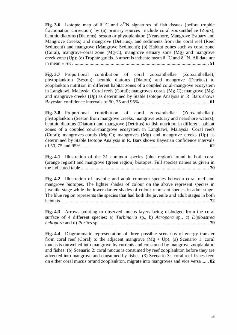
Fig. 3.6 Isotopic map of δ13

C and δ15

N signatures of fish tissues (before trophic

fractionation correction) by (a) primary sources include coral zooxanthellae (Zoox),

benthic diatoms (Diatoms), seston or phytoplankton (Nearshore, Mangrove Estuary and

Mangrove Creeks) and mangrove (Detritus), and sediments from the coral reef (Reef

Sediment) and mangrove (Mangrove Sediment); (b) Habitat zones such as coral zone

(Coral), mangrove-coral zone (Mg-C), mangrove estuary zone (Mg) and mangrove

creek zone (Up); (c) Trophic guilds. Numerals indicate mean δ13

C and δ15

N. All data are

in mean ± SE .............................................................................................................. 51

Fig. 3.7 Proportional contribution of coral zooxanthellae (Zooxanthellae);

phytoplankton (Seston); benthic diatoms (Diatom) and mangrove (Detritus) to

zooplankton nutrition in different habitat zones of a coupled coral-mangrove ecosystem

in Langkawi, Malaysia. Coral reefs (Coral); mangroves-corals (Mg-C); mangrove (Mg)

and mangrove creeks (Up) as determined by Stable Isotope Analysis in R. Bars shows

Bayesian confidence intervals of 50, 75 and 95% ........................................................ 61

Fig. 3.8 Proportional contribution of coral zooxanthellae (Zooxanthellae);

phytoplankton (Seston from mangrove creeks, mangrove estuary and nearshore waters);

benthic diatoms (Diatom) and mangrove (Detritus) to fish nutrition in different habitat

zones of a coupled coral-mangrove ecosystem in Langkawi, Malaysia. Coral reefs

(Coral); mangroves-corals (Mg-C); mangroves (Mg) and mangrove creeks (Up) as

determined by Stable Isotope Analysis in R. Bars shows Bayesian confidence intervals

of 50, 75 and 95% ....................................................................................................... 62

Fig. 4.1 Illustration of the 31 common species (blue region) found in both coral

(orange region) and mangrove (green region) biotopes. Full species names as given in

the indicated table ....................................................................................................... 70

Fig. 4.2 Illustration of juvenile and adult common species between coral reef and

mangrove biotopes. The lighter shades of colour on the above represent species in

juvenile stage while the lower darker shades of colour represent species in adult stage.

The blue region represents the species that had both the juvenile and adult stages in both

habitats……. ............................................................................................................... 72

Fig. 4.3 Arrows pointing to observed mucus layers being dislodged from the coral

surface of 4 different species: a) Turbinaria sp., b) Acropora sp., c) Diploastrea

heliopora and d) Porites sp. ....................................................................................... 79

Fig. 4.4 Diagrammatic representation of three possible scenarios of energy transfer

from coral reef (Coral) to the adjacent mangrove (Mg + Up). (a) Scenario 1: coral

mucus is outwelled into mangrove by currents and consumed by mangrove zooplankton

and fishes; (b) Scenario 2: coral mucus is consumed by reef zooplankton before they are

advected into mangrove and consumed by fishes. (3) Scenario 3: coral reef fishes feed

on either coral mucus or/and zooplankton, migrate into mangroves and vice versa ...... 82

xiii

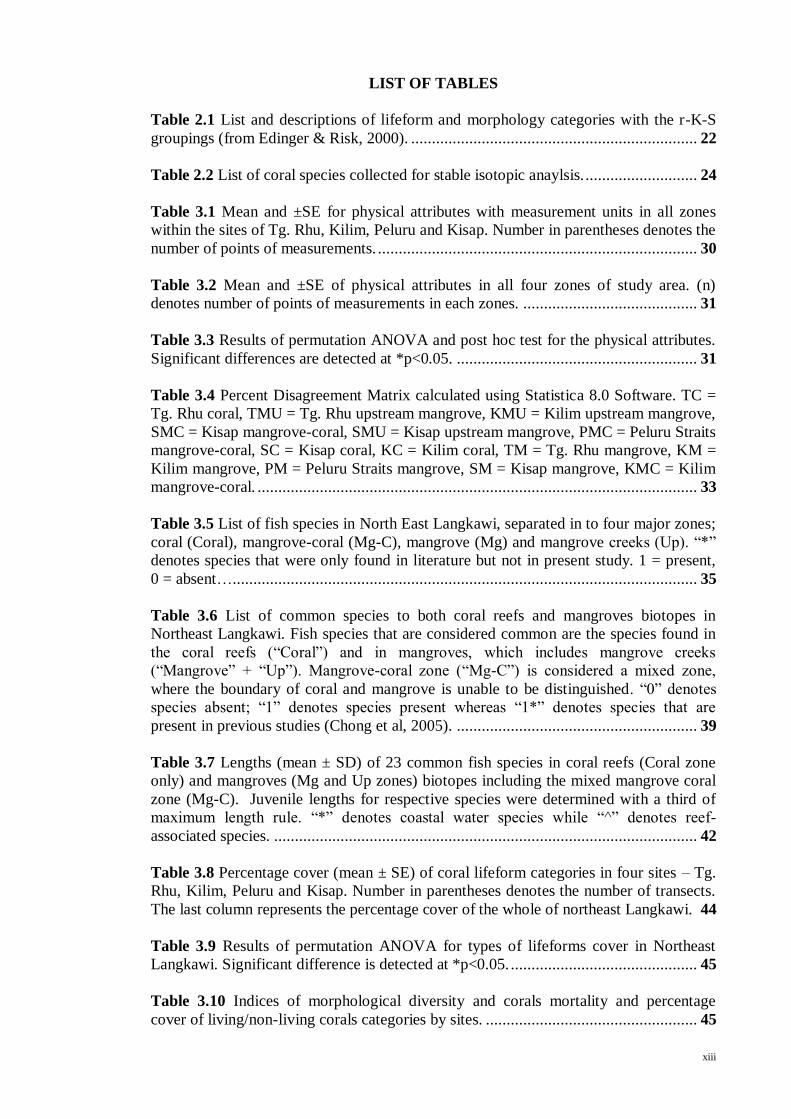
LIST OF TABLES

Table 2.1 List and descriptions of lifeform and morphology categories with the r-K-S

groupings (from Edinger & Risk, 2000). ..................................................................... 22

Table 2.2 List of coral species collected for stable isotopic anaylsis. ........................... 24

Table 3.1 Mean and ±SE for physical attributes with measurement units in all zones

within the sites of Tg. Rhu, Kilim, Peluru and Kisap. Number in parentheses denotes the

number of points of measurements. ............................................................................. 30

Table 3.2 Mean and ±SE of physical attributes in all four zones of study area. (n)

denotes number of points of measurements in each zones. .......................................... 31

Table 3.3 Results of permutation ANOVA and post hoc test for the physical attributes.

Significant differences are detected at *p<0.05. .......................................................... 31

Table 3.4 Percent Disagreement Matrix calculated using Statistica 8.0 Software. TC =

Tg. Rhu coral, TMU = Tg. Rhu upstream mangrove, KMU = Kilim upstream mangrove,

SMC = Kisap mangrove-coral, SMU = Kisap upstream mangrove, PMC = Peluru Straits

mangrove-coral, SC = Kisap coral, KC = Kilim coral, TM = Tg. Rhu mangrove, KM =

Kilim mangrove, PM = Peluru Straits mangrove, SM = Kisap mangrove, KMC = Kilim

mangrove-coral. .......................................................................................................... 33

Table 3.5 List of fish species in North East Langkawi, separated in to four major zones;

coral (Coral), mangrove-coral (Mg-C), mangrove (Mg) and mangrove creeks (Up). “*”

denotes species that were only found in literature but not in present study. 1 = present,

0 = absent…................................................................................................................ 35

Table 3.6 List of common species to both coral reefs and mangroves biotopes in

Northeast Langkawi. Fish species that are considered common are the species found in

the coral reefs (“Coral”) and in mangroves, which includes mangrove creeks

(“Mangrove” + “Up”). Mangrove-coral zone (“Mg-C”) is considered a mixed zone,

where the boundary of coral and mangrove is unable to be distinguished. “0” denotes

species absent; “1” denotes species present whereas “1*” denotes species that are

present in previous studies (Chong et al, 2005). .......................................................... 39

Table 3.7 Lengths (mean ± SD) of 23 common fish species in coral reefs (Coral zone

only) and mangroves (Mg and Up zones) biotopes including the mixed mangrove coral

zone (Mg-C). Juvenile lengths for respective species were determined with a third of

maximum length rule. “*” denotes coastal water species while “^” denotes reef-

associated species. ...................................................................................................... 42

Table 3.8 Percentage cover (mean ± SE) of coral lifeform categories in four sites – Tg.

Rhu, Kilim, Peluru and Kisap. Number in parentheses denotes the number of transects.

The last column represents the percentage cover of the whole of northeast Langkawi. 44

Table 3.9 Results of permutation ANOVA for types of lifeforms cover in Northeast

Langkawi. Significant difference is detected at *p<0.05. ............................................. 45

Table 3.10 Indices of morphological diversity and corals mortality and percentage

cover of living/non-living corals categories by sites. ................................................... 45

xiv

Table 3.11 Mean ± SE isotope values of δ13

C, δ15

N and C/N ratio of the possible

primary energy sources, zooplankton and sediments. n denotes the number of samples

collected for each source. *from Okamura et al. (2010). .............................................. 50

Table 3.12 Results of Kruskal-Wallis non-parametric test and post hoc Wilcoxon

Mann-Whitney test. Significant difference are at *p<0.001. Pairs of insignificant

difference are denoted by the same letters ................................................................... 52

Table 3.13 Mean and ±SE tissues isotopes of δ13

C, δ15

N (both expressed in ‰) and C/N

ratio of fish species (grouped into respective feeding guilds) with number of samples

collected (n) in each zone. ........................................................................................... 55

Table 3.14 Mean ± SE isotopes of δ13

C, δ15

N and C/N ratio of fish tissues pooled

according to different habitat zones where they were collected; coral reefs (Coral);

mixed mangroves-coral (MgC); mangrove estuary (Mangrove) and mangrove creeks

(Up). n = number of samples. ...................................................................................... 60

xv

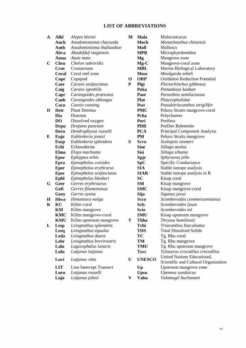
LIST OF ABBREVIATIONS

A Alkl Alepes kleinii M Mala Malacostracas

Anch Anodontostoma chacunda Moch Monachanthus chinensis

Anth Anodontostoma thailandiae Moll Molluscs

Abva Abudefduf vaigiensis MPB Microphytobenthos

Atma Atule mate Mg Mangrove zone

C Chsu Chelon subviridis Mg-C Mangrove-coral zone

Crus Crustaceans MBL Marine Biological Laboratory

Coral Coral reef zone Mose Moolgarda seheli

Cope Copepod O ORP Oxidation Reduction Potential

Case Caranx sexfasciatus P Plgi Plectorhinchus gibbosus

Caig Caranx ignobilis Poka Pomadasys kaakan

Capr Carangoides praeustus Pase Paranibea semiluctuosa

Caob Carangoides oblongus Plat Platycephalidae

Cacu Caesio cunning Psst Pseudotriacanthus strigilifer

D Detr Plant Detritus PMC Peluru Straits mangrove-coral

Dia Diatoms Pcha Polychaetes

DO Dissolved oxygen Pori Porifera

Drpu Drepane punctate PDB PeeDee Belemnite

Deru Dendrophyssa russelli PCA Principal Component Analysis

E Eujo Eubleekeria jonesi PM Peluru Straits mangrove

Eusp Eubleekeria splendens S Scvo Scolopsis vosmeri

Echi Echinoderms Siae Sillago aeolus

Elma Elops machnata Sisi Sillago sihama

Epor Ephippus orbis Spje Sphyraena jello

Epco Epinephelus coioides SpC Specific Conductance

Eper Epinephelus erythrurus SIA Stable isotope analysis

Epse Epinephelus sexfasciatus SIAR Stable isotope analysis in R

Epbl Epinephelus bleekeri SC Kisap coral

G Geer Gerres erythrourus SM Kisap mangrove

Gefi Gerres filamentosus SMC Kisap mangrove-coral

Geoy Gerres oyena Sija Siganus javus

H Hiwa Himantura walga Scco Scomberoides commersonnianus

K KC Kilim coral Scly Scomberoides lysan

KM Kilim mangrove Scto Scomberoides tol

KMC Kilim mangrove-coral SMU Kisap upstream mangrove

KMU Kilim upstream mangrove T Thha Thryssa hamiltonii

L Lesp Leiognathus splendens Trbi Triacanthus biaculeatus

Leeq Leiognathus equulus TDS Total Dissolved Solids

Leda Leiognathus daura TC Tg. Rhu coral

Lebr Leiognathus brevirostris TM Tg. Rhu mangrove

Lalu Lagocephalus lunaris TMU Tg. Rhu upstream mangrove

Lulu Lutjanus lutjanus Tycc Tylosurus crocodilus crocodilus

Luvi Lutjanus vitta U UNESCO United Nations Educational,

Scientific and Cultural Organization

LIT Line Intercept Transect Up Upstream mangrove zone

Luru Lutjanus russelli Upsu Upeneus sundaicus

Lujo Lutjanus johnii V Vabu Valamugil buchanani

xvi

LIST OF APPENDICES

APPENDIX I List of fish species caught at 4 sites in Northeastern Langkawi (Fig.

2.1). “0” denotes absent and “1” denotes present. “1*” denotes species present from

literature (Chong, 2005). ............................................................................................. 98

APPENDIX II Details of PCA on dietary composition of fish species computed in

Canoco software.... ................................................................................................... 104

APPENDIX III Results of the non-parametruc Kruskal-Wallis analysis on stable

isotope signatures…. ................................................................................................. 105

APPENDIX IV Results of 95%, 75% and 50% probability and mean values of

proportional source contribution to zooplankton in each habitat zone as determined by

SIAR.............. ……. .................................................................................................. 106

APPENDIX V Results of 95%, 75% and 50% probability and mean values of

proportional source contribution to fish in each habitat zone as determined by SIAR 107

APPENDIX VI Dietary composition of fish species used for computing PCA in

Canoco software…...… ............................................................................................. 108

APPENDIX VII Fish stable isotope signatures for carbon, δ13

C and nitrogen, δ15

N

with trophic fractionation correction for carbon, ∆13

C and nitrogen, ∆15

N used in

computing SIAR…….. ............................................................................................. 111

APPENDIX VIII Commands for computing SIAR package in R. ............................ 119

APPENDIX IX Commands for computing Permutation ANOVA and t-test in R .. 120

APPENDIX X Summary of permutation ANOVA test computed in R ................ 121

1

1.0 INTRODUCTION

1.1 What is connectivity?

In the large oceanic environments throughout the world, marine habitats or

biotopes such as coral reefs, mangroves and seagrass meadows are usually patchily

distributed. Due to the nature of such geographically patchy distributions, each biotope

is separated by seawater. The spaces or gaps between biotopes provide transportation

routes, like a “blue highway” (Kelley & Ryan, 2000). Through this blue highway, items

such as nutrients, organic matter, sediments, pollutants, energy, organisms and even

genes can regulate between biotopes, either of the same or different types. Such

regulation forms a connection between biotopes, which is termed as connectivity.

In general, connectivity can be divided into two different forms, namely, genetic

connectivity and ecological connectivity (Nagelkerken, 2009a; Sale et al., 2010). While

genetic connectivity mostly involves the flow of genes among populations between

biotopes, ecological connectivity, which requires a more complex understanding refers

to exchanges of nutrients, organic matter or abiotic materials and also movements of

living organism between biotopes (Nagelkerken, 2009a; Sale et al., 2010). In the

context of the present study, ecological connectivity is studied and focused on the coral

reef and mangrove biotopes.

1.2 Ecological connectivity of biotopes

There are three ways that adjacent disparate biotopes such as coral reef and

mangrove are ecologically connected. They can either be physically, biogeochemically

or biologically connected. Physical connectivity involves sediment transfers, flow

regulations and hydrodynamic processes such as waves, currents, tidal changes and

water body movements (Ogden & Gladfelter, 1983; Wolanski, 2001). Biogeochemical

connectivity on the other hand involve exchanges of nutrients and organic matters

2

between biotopes. Biological connectivity is probably the most complicated, involving

the study of life-cycles, nursery habitats, trophodynamics, movements and migrations of

organisms (Sheaves, 2005, 2009). Although all three forms of connectivity are strongly

related, this present study mainly focuses on biological connectivity, particularly on the

marine ichthyofauna.

Movement of marine fauna between biotopes is the most conspicuous

component of biological connectivity (Sheaves, 2009). Several studies on connectivity

involving movement or migration of marine fauna have been conducted in the past.

These include the juvenile and adult habitat connectivity among mobile fauna

(Gillanders, Able, Brown, Eggleston, & Sheridan, 2003), connectivity between fish in

seagrass beds, mangroves and coral reefs (Dorenbosch, 2006; Jaxion-Harm, Saunders,

& Speight, 2012), seagrass fish assemblages adjacent to mangroves and coral reefs

(Unsworth et al., 2008) and ontogenetic migration of Lutjanus fulvus, L. johnii and

several other coral reef fishes between habitats (Jones, Walter, Brooks, & Serafy, 2010;

Nakamura et al., 2008; Tanaka et al., 2011). Many of these studies have shown that

marine fauna, in particular fish, utilised more than one habitat during their life cycle,

either for nursery, shelter or for feeding. Such connectivity is crucial in ensuring the

survival of fish larvae, enhancing fish biomass, structuring populations, maintaining

food web dynamics and even increasing the resilience of habitats to natural disasters

(Mumby & Hastings, 2008; Mumby et al., 2004; Sheaves, 2009).

1.3 Coral reefs

Coral reefs are basically a framework of calcareous structures built mostly by

reef building corals known as scleractinian (hard) corals, hence the name. Coral reefs

are dynamic systems and they influence the oceans’ chemical balance due to their

ability to take in and temporarily bind calcium that enters sea water, which in turn each

3

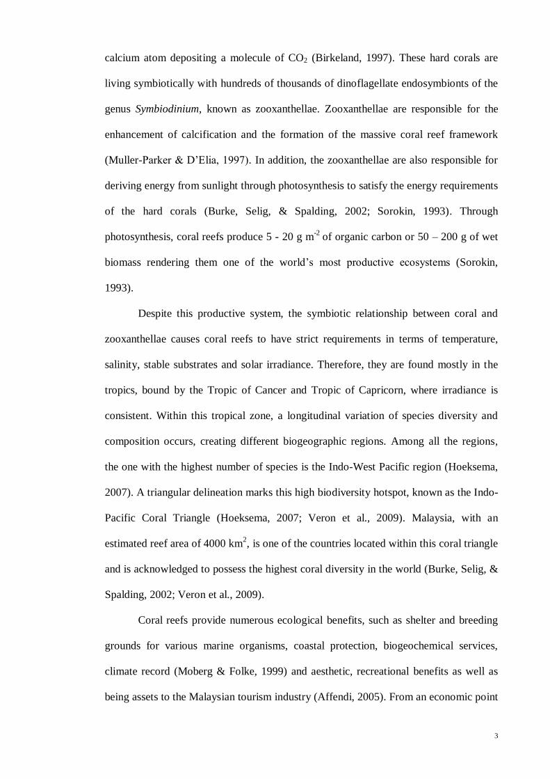
calcium atom depositing a molecule of CO2 (Birkeland, 1997). These hard corals are

living symbiotically with hundreds of thousands of dinoflagellate endosymbionts of the

genus Symbiodinium, known as zooxanthellae. Zooxanthellae are responsible for the

enhancement of calcification and the formation of the massive coral reef framework

(Muller-Parker & D’Elia, 1997). In addition, the zooxanthellae are also responsible for

deriving energy from sunlight through photosynthesis to satisfy the energy requirements

of the hard corals (Burke, Selig, & Spalding, 2002; Sorokin, 1993). Through

photosynthesis, coral reefs produce 5 - 20 g m-2

of organic carbon or 50 – 200 g of wet

biomass rendering them one of the world’s most productive ecosystems (Sorokin,

1993).

Despite this productive system, the symbiotic relationship between coral and

zooxanthellae causes coral reefs to have strict requirements in terms of temperature,

salinity, stable substrates and solar irradiance. Therefore, they are found mostly in the

tropics, bound by the Tropic of Cancer and Tropic of Capricorn, where irradiance is

consistent. Within this tropical zone, a longitudinal variation of species diversity and

composition occurs, creating different biogeographic regions. Among all the regions,

the one with the highest number of species is the Indo-West Pacific region (Hoeksema,

2007). A triangular delineation marks this high biodiversity hotspot, known as the Indo-

Pacific Coral Triangle (Hoeksema, 2007; Veron et al., 2009). Malaysia, with an

estimated reef area of 4000 km2, is one of the countries located within this coral triangle

and is acknowledged to possess the highest coral diversity in the world (Burke, Selig, &

Spalding, 2002; Veron et al., 2009).

Coral reefs provide numerous ecological benefits, such as shelter and breeding

grounds for various marine organisms, coastal protection, biogeochemical services,

climate record (Moberg & Folke, 1999) and aesthetic, recreational benefits as well as

being assets to the Malaysian tourism industry (Affendi, 2005). From an economic point

4

of view, it has been estimated that in South East Asia, coral reefs provide an annual net

value of between RM 75,000 to RM 900,000 per square kilometre which includes

tourism, fisheries and coastal protection (Burke et al., 2002). On the West Coast of

Peninsular Malaysia, the total annual economic value of coral reefs has been estimated

to be RM 41,407 per hectare of coral reef (MPP-EAS, 1999).

1.4 Mangroves

Mangrove habitats or mangals naturally exist on the boundary between

terrestrial and the saline sea environment. They are globally distributed only within the

latitude of 23.5°N and 23.5°S making them almost exclusively tropical, similar to the

coral reefs. Their latitudinal restriction is related to seawater temperature, which is

delimited by a 20°C isotherm during winter (Hogarth, 2007). Besides being globally

limited by temperature, mangroves are also subjected to local physiological constraints

such as rainfall, tidal regime, wave actions and river flow (Alongi, 2009). As a key

ecosystem occupying the harsh conditions between terrestrial and marine environment,

mangroves are fairly robust and highly adaptable to saline and inundated conditions

(Alongi, 2008).

One of the most notable adaptations of mangrove is the root architecture system

such as prop roots, knee roots and pneumatophores. Not only are these root systems

effective in gaseous transport in water-logged and anaerobic conditions, they are also

able to exclude salt during water uptake. In addition, mangrove roots provide anchorage

in unstable muddy soil, turning the soil into hard substrate while increasing the surface

area for various fauna (Hogarth, 2007). Mangrove roots also host many epibionts and

invertebrates such as annelid worms, arthropods, molluscs and crustaceans (Hogarth,

2007; Sasekumar & Ooi, 2005). Some of this fauna, particularly herbivorous crabs, are

able to break down mangrove leaves to litter which is subsequently decomposed to

5

detritus by microbes (Hogarth, 2007). The decomposed leaves contribute to the detritus

food chain rendering mangrove to be regarded as a productive feeding ground for

various marine fauna. The complex mangrove root system with substantial food

provision serves as a suitable nursery ground for fish communities (Laegdsgaard &

Johnson, 2001).

In addition to the nursery ground function, mangroves also function as a buffer

to erosion, sedimentation, storm, waves and tsunamis. Besides providing ecological

functions and coastal protection, Peninsular Malaysia’s mangroves’ worth of RM 3.4

billion or RM 41,407 per hectare proves that they are also economically important

(MPP-EAS, 1999). Despite the fact that mangroves have such important functions and

values, we are on the verge of losing them mostly due to irresponsible coastal

development and aggravated by natural disasters such as storms and tsunamis. This

development has caused a loss of approximately a third of the world’s mangrove in five

decades (Alongi, 2002). Meanwhile in Malaysia, an estimated total of 59,543 ha or 14%

of mangrove reserves were lost between 1984 and 2004 (Chong, 2007a; Chong, Lee, &

Lau, 2010).

1.5 Physical attributes of seawater and habitat complexity

The condition of seawater is important to determine the suitability of a habitat

for living marine organisms. Changes in the seawater’s physical attributes provide

insights to any environmental changes that may be detrimental to the biotopes and the

associated marine organisms. Environmental changes can happen due to local

anthropogenic activities or natural events such as daily tidal changes or the El-Niño

phenomena (Alongi, 2008; Glynn, 1997; Hoegh-Guldberg et al., 2009). On a global

level, both coral reefs and mangroves are subjected to larger scale impacts by events

6

such as rising temperature and ocean acidification (Hoegh-Guldberg et al., 2009; Veron,

et al., 2009).

Coral reefs are sensitive and susceptible to environmental changes, in contrast to

the robust and highly tolerant mangrove (Alongi, 2008; Kleypas, McManus, & Menez,

1999). Due to the different tolerance limits of mangroves and coral reefs, it is necessary

to examine the physical attributes that distinguish the water body of both biotopes.

Temperature and pH are most important attributes, because these are indicators for

ocean warming and acidification respectively. Salinity is also a crucial attribute,

because it can influence the species and type of organisms that resides in the habitat.

Turbidity is another important attribute particularly in coral reefs because the sediment

particles, plankton and even microscopic organisms within the water column scatter

sunlight and thus reduce the penetration of light required by the corals for

photosynthetic processes (Rogers, 1990). On the other hand, turbid water provides

higher chance for fish survival because it functions well as a shelter from visual

predators (Benfield & Minello, 1996).

An important element of reducing predation risk for fish besides turbid water is

structural or habitat complexity. A habitat with higher complexity will attract more

fishes due to the higher availability of shelter to avoid predation (Gratwicke & Speight,

2005) and the provision of food resources (Nagelkerken, 2009b; Nagelkerken et al.,

2008). In addition, the physical structures of habitat can interact with various complex

ecological processes, consequently influencing the assemblages of fish communities

and their interaction with predators (Caley & St John, 1996). Habitat complexity has

also been found to influence fish preference on habitat selection, such as larval

settlement and recruitment (Nakamura, Kawasaki, & Sano, 2007). As for mangroves,

fishes are shown to be attracted to the structural complexity and shade in mangrove

7

habitats (Cocheret de la Morinière, Nagelkerken, van der Meij, & van der Velde, 2004;

Nagelkerken et al., 2010; Verweij et al., 2006).

For the present study, the focus on habitat complexity is restricted to coral reefs

and the scope will cover only the provision of sufficient shelter or refugia. Habitat

complexity of coral reefs is referred to as the reef health condition and structural

complexity. A healthy reef condition is determined through a combination of several

measures - ecological strategy of corals, live coral cover, mortality index and the

morphological diversity of corals, which will also be used as an index for habitat

complexity in the coral reefs (Edinger & Risk, 2000).

Overall, physical attributes and habitat complexity are some of the factors

influencing the utilization of both coral reefs and mangroves by marine fauna

particularly fishes. The combination of both factors will ultimately provide important

evidence to prove the presence of an ecological connectivity between these two

biotopes. The juxtaposition of factors affecting the habitat conditions of coral reefs and

mangroves can provide explicit information on how connectivity is facilitated. For

instance, extreme physical attributes, unhealthy conditions and high predation risk in a

habitat can cause marine fauna to avoid that habitat and influence their distribution,

which consequently will disrupt ecological connectivity. Conversely, a good condition

of habitat can attract more fauna, widen their spatial distribution, influence their

resource partitioning and ultimately preserve a high biodiversity.

1.6 Source contribution

Coral reef and mangrove biotopes that occur in close proximity will usually

form a complex ecosystem with ecological connectivity (Dorenbosch et al., 2005;

Nagelkerken, 2007; Unsworth et al., 2008; Jones et al., 2010; Grol et al., 2011). In a

complex ecosystem, mangroves are known to serve as nursery ground for reef fishes,

8

providing food and shelter to their juveniles (Sheaves, 2005; Grol et al., 2011; Tanaka et

al., 2011). Among the functions of nursery grounds, food provision by mangrove to reef

fishes has been given the most attention (Nagelkerken et al., 2000; Laegdsgaard and

Johnson, 2001; Chong, 2007; Tanaka et al., 2011). The major contributor of food

sources to the fish community is often believed to be mangrove detritus, via direct or

indirect trophic pathways (Nakamura et al., 2008; Sheaves, 2005). Other studies have

revealed that various sources like phytoplankton and microphytobenthos (MPB) can

also contribute significantly in mangrove habitats (Bouillon, Mohan, Sreenivas, &

Dehairs, 2000), especially to the zooplankton and small nekton community (Chew,

Chong, Tanaka, & Sasekumar, 2012). However, in other coupled biotopes, such as

mangroves with seagrass beds, it appears that the mangroves’ contribution to the fish

food web is marginal compared to the seagrass beds (Lugendo, Nagelkerken, van der

Velde, & Mgaya, 2006; Marguillier, van der Velde, Dehairs, Hemminga, & Rajagopal,

1997; Nagelkerken & van der Velde, 2004a; Nyunja et al., 2009). This has been

attributed to the poor nutritional value of mangrove detritus, which is low in nitrogen,

i.e. high C/N ratio (Wolcott & O’Connor, 1992). Consumers are likely to shift their

food preference to more nutritious ones if available. Moreover, most fishes cannot

digest the largely lignin-cellulosic component of mangrove detritus (Wolcott &

O’Connor, 1992).

Compared to mangrove – seagrass bed connectivity, there is a paucity of

information on the trophic contribution of tropical coral reefs to mangrove and vice-

versa. Coral derived organic matter, largely in the form of mucus released into the water

column, is considered relatively nutritious due to its high protein content or lower C/N

ratio (Coles & Strathmann, 1973; Johannes, 1967; Wyatt, 2011). Coral mucus contains

nutrient rich components of lipids, triglycerides and proteins (Benson & Muscatine,

1974; Coles & Strathmann, 1973; Ducklow & Mitchell, 1979) and consequently has

9

been proposed as one of the energy transfer pathways from coral hosts and their

zooxanthellae to the reef consumers (Benson & Muscatine, 1974; Ducklow & Mitchell,

1979; Richman, Loya, & Slobodkin, 1975). The coral mucus aggregates to form

suspended flocs that are able to trap organic particles including bacteria (Naumann,

Richter, el-Zibdah, & Wild, 2009; Wild, Huettel, Klueter, & Kremb, 2004), further

enhancing their nutritional value (Johannes, 1967). The nutritional values are evident as

mucus is consumed by various reef-associated fauna such as fishes, crabs, shrimps,

zooplanktons and even benthic invertebrates (Benson & Muscatine, 1974; Johannes,

1967; Naumann, Mayr, Struck, & Wild, 2010; Richman et al., 1975). For example, in an

oligotrophic subtropical reef such as Heron Island, coral mucus flocs have been

hypothesized to fuel the benthic and pelagic food chains (Wild et al., 2004). Although

coral mucus contribution is apparent in the food web of subtropical nutrient-poor coral

reefs, its contribution in tropical coupled coral reef and mangrove biotopes is largely

unknown. In such tropical coupled systems where turbidity and dissolved inorganic

nutrients are usually higher, the trophic inputs from phytoplankton, MPB and mangrove

detritus may be equivocal.

Fish are highly diverse in trophic groups and feeding strategies, making their

community highly complex, particularly when they utilize different habitats that occur

adjacent to each other. Various studies have provided evidence of trophic links between

mangroves and adjacent habitats through fish movements as a result of life cycle

requirements, especially relating to ontogenetic shifts (Mumby et al., 2004; Nakamura

et al., 2008; Unsworth et al., 2008; Jones et al., 2010; Tanaka et al., 2011). Most of

these studies however have focused on only one or a few species, while investigations at

the community level with high numbers of species are unfortunately lacking. Such

studies are more likely to provide comprehension of broad-scale trophic connectivity

10

and interdependency between coral reefs and mangroves (Polis, 1994; Abrantes and

Sheaves, 2009).

1.7 Stomach content and stable isotope analysis

Traditional stomach content analysis assesses the consumer’s diet over a short

temporal scale of up to a few hours of recently ingested food and is able to provide a

diet description and determine feeding guilds (Cocheret de la Morinière et al., 2003;

Drazen et al., 2008). However, stable isotope analysis (SIA) has increasingly been used

in ecological studies, especially those related to the trophodynamics of various marine

ecosystems including connected habitats (Chew et al., 2012; Nagelkerken & van der

Velde, 2004b; Nakamura et al., 2008; Tanaka et al., 2011; Wyatt, Waite, & Humphries,

2012). SIA discriminates the heavier isotope of carbon (13

C) and nitrogen (15

N) in the

metabolic pathways of the consumers’ tissues. The measurements of heavy to light

isotopes ratio of carbon (13

C/12

C) and nitrogen (15

N/14

N), in the unit of ‰ (parts per

million), denoted as δ13

C and δ15

N respectively, are the basis of tracing the sources and

trophic pathways in ecological communities (Peterson & Fry, 1987; Hobson &

Wassenaar, 1999; Zanden & Rasmussen, 2001). It is generally accepted that δ15

N is

greatly enriched at successive trophic levels thus allowing it to estimate consumer’s

trophic position. On the other hand δ13

C, only marginally enriched with trophic transfer,

determines the primary sources of consumers’ diets (McCutchan, Lewis, & McGrath,

2003; Minagawa & Wada, 1984; Post, 2002; Vander Zanden & Rasmussen, 2001).

Based on this concept, one of the most common applications of SIA is the use of the

Bayesian mixing model to estimate the contribution of each primary source (Parnell,

Inger, Bearhop, & Jackson, 2010).

11

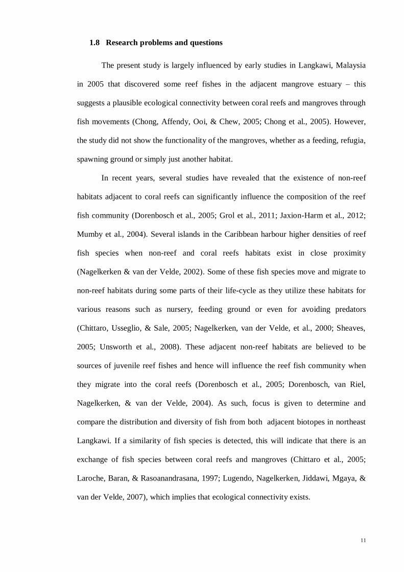
1.8 Research problems and questions

The present study is largely influenced by early studies in Langkawi, Malaysia

in 2005 that discovered some reef fishes in the adjacent mangrove estuary – this

suggests a plausible ecological connectivity between coral reefs and mangroves through

fish movements (Chong, Affendy, Ooi, & Chew, 2005; Chong et al., 2005). However,

the study did not show the functionality of the mangroves, whether as a feeding, refugia,

spawning ground or simply just another habitat.

In recent years, several studies have revealed that the existence of non-reef

habitats adjacent to coral reefs can significantly influence the composition of the reef

fish community (Dorenbosch et al., 2005; Grol et al., 2011; Jaxion-Harm et al., 2012;

Mumby et al., 2004). Several islands in the Caribbean harbour higher densities of reef

fish species when non-reef and coral reefs habitats exist in close proximity

(Nagelkerken & van der Velde, 2002). Some of these fish species move and migrate to

non-reef habitats during some parts of their life-cycle as they utilize these habitats for

various reasons such as nursery, feeding ground or even for avoiding predators

(Chittaro, Usseglio, & Sale, 2005; Nagelkerken, van der Velde, et al., 2000; Sheaves,

2005; Unsworth et al., 2008). These adjacent non-reef habitats are believed to be

sources of juvenile reef fishes and hence will influence the reef fish community when

they migrate into the coral reefs (Dorenbosch et al., 2005; Dorenbosch, van Riel,

Nagelkerken, & van der Velde, 2004). As such, focus is given to determine and

compare the distribution and diversity of fish from both adjacent biotopes in northeast

Langkawi. If a similarity of fish species is detected, this will indicate that there is an

exchange of fish species between coral reefs and mangroves (Chittaro et al., 2005;

Laroche, Baran, & Rasoanandrasana, 1997; Lugendo, Nagelkerken, Jiddawi, Mgaya, &

van der Velde, 2007), which implies that ecological connectivity exists.

12

A recent study in Matang Mangrove Forest, Malaysia showed evidence that

mangroves function as nursery area mainly due to the easily available food resource for

certain reef fishes (Tanaka et al., 2011). However, other studies in the Indo-Pacific

region suggested otherwise where the function of mangroves as nursery ground is

relatively minor and the connectivity was said to be less significant (Huxham, Kimani,

& Augley, 2004; Laroche et al., 1997). Although there are studies that reported the

presence of juvenile reef fishes in the mangroves, their function as nursery ground is

still largely unclear. The mangroves could serve as refugia, spawning or feeding

grounds or simply another habitat, but there is insufficient evidence to prove these

functionalities. Thus, the non-reef habitat function as nursery ground is not necessarily

true in all cases (Chittaro et al., 2005).

With regards to refugia, it is already generally accepted that mangroves provide

refuge for fishes (Sheaves, 2005). Therefore, fishes will face higher predation risk if

they swim out of the mangroves and into the coral reefs. However, if coral reefs can

provide substantial refuge cover, fishes can utilise coral reefs during low tide, when

mangroves are not fully inundated. The question of how much cover coral reefs can

provide to the fish communities can be answered through examining the habitat

complexity of the coral reef. This contributes to habitat connectivity and optimizes the

fish trade-off strategy between predation risk and food availability (Grol et al., 2011).

Food availability is another aspect that contributes to biotope connectivity, which gives

rise to the question of the primary source of food contribution to the fish community. To

answer this, both stomach content analysis and the SIA approach will be used in the

present study.

Most studies in other parts of the world have shown that connectivity exists

between coastal habitats and provides mutual benefits to the connected ecosystems.

However, the functionality of the connected habitats varies between locations and

13

provides different contributions to the fish community. Regardless, the important

factors that determine the functionality of connected habitats as nursery or feeding area

are the availability of food source and refuge space. Clearly, habitat connectivity studies

are still lacking, especially in the Indo-Pacific region as compared to the extensive

works done in the Caribbean region, (Dorenbosch, 2006). Therefore, there is a need for

this kind of study in Malaysia where several coastal biotopes often co-occur close to

each other, while the management of these biotopes is under the jurisdiction of different

government agencies.

1.9 Significance of study

The co-occurrence of disparate habitats such as coral reefs which are intolerant

to high total suspended solids and turbid water mangroves within one general area is

quite rare in Malaysia. The present study site in the northeast of Langkawi Island,

Kedah is one of the few while other sites are located in Merambong Shoal, Johor; Seri

Buat Island, Pahang and Banggi Island, Sabah in East Malaysia. These unique co-

occurring habitats have the potential to substantially contribute to the whole ecosystem

and its associated fauna. However, with the rapid development along the coastlines in

these locations, these unique co-occurring habitats are at risk of being lost. There is an

alarming concern that the hinterland in Langkawi is developing rapidly along with the

removal of mangrove forests (Shahbudin, Zuhairi, & Kamaruzzaman, 2012) and the

increased terrestrial downstream flow to the coral reefs (Jalal et al., 2009).

Coral reefs and mangroves are among the two most productive ecosystems, rich

in biodiversity and able to provide various ecological services. These two biotopes,

along with seagrass beds, are estimated to be able to support the livelihood of 275

million people from 100 developed countries that are dependent on coastal resources

(Wilkinson & Salvat, 2012). In the past few decades, mangroves and coral reefs have

14

suffered severe degradation due to various human pressures and natural impacts.

Approximately 35% of the world’s mangroves have been lost in over two decades due

to aquaculture, deforestation and freshwater diversion (Mooney et al., 2005), and on top

of that mangroves continue to face an average annual loss rate of 1 to 2% (Alongi,

2008). Likewise, coral reefs have suffered loss of 19% and it is estimated that a further

35% face the risk of being impacted directly by anthropogenic pressure (Wilkinson,

2008; Wilkinson & Salvat, 2012). The risk of coral reef degradation is estimated to have

increased by up to 75% if local threats are combined with rising global temperature

(Burke, Reytar, Spalding, & Perry, 2011). Due to these threats and risks, an urgency in

the protection and conservation of these valuable biotopes is desperately needed. Most

conservation efforts have focused on single biotope independently instead of the whole

entity of interconnected coupled biotopes (Nagelkerken, 2009b). An integrated

protection and management of such complex interconnected biotopes is imperative in

order to maintain the biodiversity and ecological services they provide (McCook et al.,

2009).

In Malaysia, coral reefs and mangroves are independently managed by different

government departments - the coral reefs by the Marine Parks Department while

mangroves are under the jurisdiction of the Forestry Department. The different

jurisdictions create difficulties for simultaneously managing both habitats. With regard

to rapid development rate along the coastlines, independent management only causes

delay and ineffective response in addressing mangrove forest removal and pollution or

sedimentation of the coral reefs. This study will provide additional information for the

promotion of integrated management for both habitats simultaneously.

As mentioned in the previous sections, studies in other parts of the world have

provided some evidence that coral reefs and mangroves are somehow connected. This

includes fish movements and trophic linkage connecting the physically separate habitats

15

of coral reefs and mangroves. However, one of the concerns is that the connectedness

between corals and mangroves may be severed due to the fast growing development. In

addition to that, independent management can disrupt the connectivity between habitats

because it does not concurrently address both habitats. Hence, there is a need to

elucidate this possible connectivity between the habitats. This study could provide the

scientific knowledge necessary for improving the design of management strategies and

protection measures.

1.10 Hypotheses and objectives

Chong et al. (2005) discovered the presence of similar fish species in both the

coastal open waters and the mangroves in Langkawi and suggested the possibility of

ecological connectivity between the mangroves and its closest adjacent biotope, coral

reefs. However, due to the short nature of the study, they could not determine the nature

of the connectivity. Thus, to continue this earlier work, the present study tested the

following two hypotheses regarding the coral reefs and mangroves of Northeast

Langkawi Island:-

1) The biotopes are ecologically connected via habitat utilisation by the fish fauna

2) The biotopes are ecologically connected via trophic energy pathways.

In order to test the two hypotheses, the study had the following objectives:-

i) To determine and compare the diversity and similarity of fish communities in the

coral reefs and mangroves

ii) To determine the habitat complexity of coral reef for fish fauna utilisation

iii) To trace the trophic pathway from primary sources to consumers using stable

isotope analysis

16

2.0 METHODOLOGY

2.1 Study site and habitat zoning

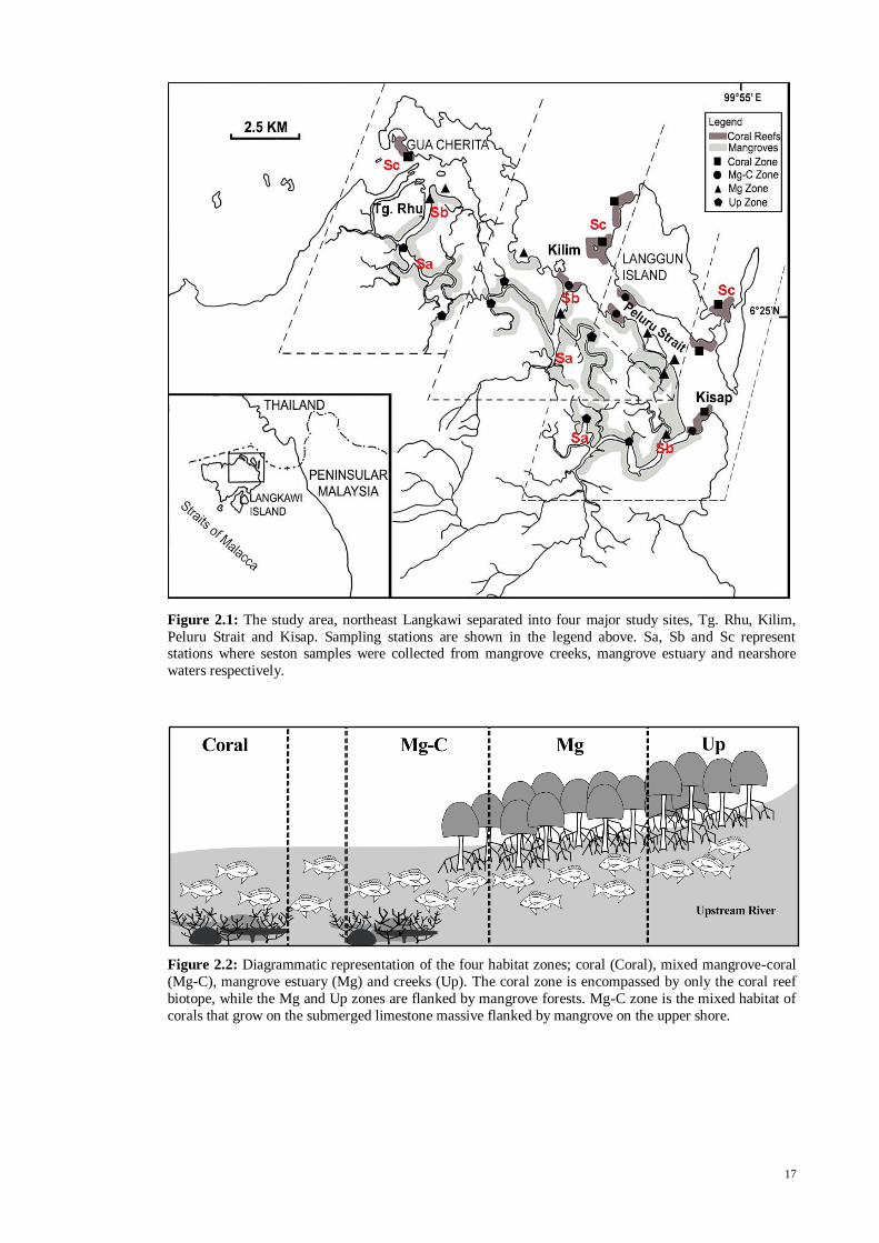
The study area was located at the northeast of Langkawi Island, Malaysia (Fig.

2.1). The area forms part of the Kilim Limestone Karst Geoforest Park (henceforth

mentioned as Kilim), the first geopark in Southeast Asia declared by UNESCO in 2007.

The geopark has approximately 1,987 ha of mangroves and patchy fringing coral reefs

around the near-shore islands of Langgun Island and Dendang Island, and the rocky

promontory of Gua Cherita, which cover an approximate total area of 40 ha. The

mangroves which grow on limestone karst have been classified as Thom (1984)’s Type

IV mangrove (Chong et al., 2005), dominated by Rhizophora apiculata and Ceriops

tagal (Sasekumar & Ooi, 2005). The coral reefs appear to thrive despite the relatively

turbid water (maximum horizontal visibility of 2 m) with live hard coral cover ranging

from 26 to 58% (Affendi, 2005).

Sampling stations were established at four major sites determined by the

estuarine drainage systems of the Rhu, Kilim and Kisap rivers and coastal water of the

Peluru Strait. Each site could be further separated into four zones of sampling (Fig. 2.2),

namely, coral reef (Coral), mixed mangrove-coral (Mg-C), mangrove estuary (Mg) and

mangrove creeks (Up). “Coral” denotes the zone that is strictly coral reef area only.

“Mg-C” is the zone at the river mouth where mangroves and corals are in close

proximity and the boundary could not be easily distinguished. “Mg” refers to the zone

restricted to mangroves area only, usually within the river, but upstream from the river

mouth. “Up” refers to the mangrove creek zone that is to the farthest upstream portion

of the river.

17

Figure 2.1: The study area, northeast Langkawi separated into four major study sites, Tg. Rhu, Kilim,

Peluru Strait and Kisap. Sampling stations are shown in the legend above. Sa, Sb and Sc represent stations where seston samples were collected from mangrove creeks, mangrove estuary and nearshore

waters respectively.

Figure 2.2: Diagrammatic representation of the four habitat zones; coral (Coral), mixed mangrove-coral

(Mg-C), mangrove estuary (Mg) and creeks (Up). The coral zone is encompassed by only the coral reef

biotope, while the Mg and Up zones are flanked by mangrove forests. Mg-C zone is the mixed habitat of

corals that grow on the submerged limestone massive flanked by mangrove on the upper shore.

18

Notably, only Kilim and Kisap contain all four zones, while Tg. Rhu has three

zones (Coral, Mg and Up) and Peluru Strait has only two zones (Mg-C and Mg). In Tg.

Rhu, the Mg-C zone was non-existent in their geographical structure and thus could not

be established. Similarly in Peluru, the Coral and Up zones could not be established. Tg.

Rhu, Kilim and Kisap are the estuarine drainage systems on the main island, while the

Peluru Strait is the coastal channel located between the main island and Langgun Island.

Hence, a total of 13 stations in four sites were established for the present study. The

nearest distances between the coral reef and the river mouth of Rhu, Kilim and Kisap

are 1.6, 0.4 and 0.7 km respectively. The farthest stations of sampling in the Up zone of

the Tg. Rhu, Kilim and Kisap sites were located 6.0, 5.5 and 5.0 km upstream from the

river mouth, respectively. Samplings in Peluru Strait were done in the coastal inlets and

bay on both sides of the channel. The zoning for each site was created to determine the

range of habitats in which fish species were found. This will give an indication of the

habitats that a fish species utilised in the area.

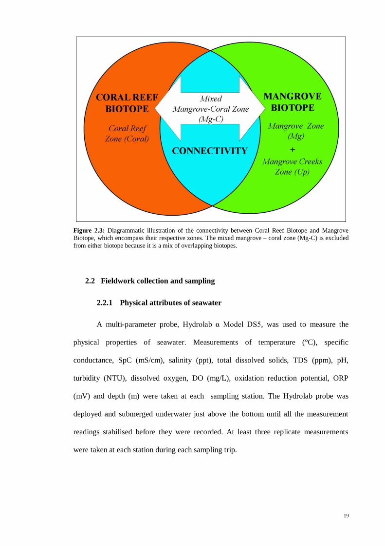
Although each site was zoned, there was still a need to categorize the zone as the

coral reef or mangrove biotope, which was the aim of the present study. Thus, the coral

reef biotope encompasses only the “Coral” zone while the mangrove biotope

encompasses the “Up” and “Mg” zones. Due to the difficulty of distinguishing the

distinct boundary of the “Mg-C” zone, this zone was not assigned to any one biotope

but rather as a mix of overlapping coral reef and mangrove biotopes (Fig. 2.3). Fishes

caught in this zone were difficult to determine as whether strictly coral or strictly

mangrove species. The term “common fish” in the present study refers to the fish

species that were found in both coral reef (“Coral”) and mangrove (“Mg” and “Up”)

biotopes (Fig. 2.3).

19

Figure 2.3: Diagrammatic illustration of the connectivity between Coral Reef Biotope and Mangrove

Biotope, which encompass their respective zones. The mixed mangrove – coral zone (Mg-C) is excluded

from either biotope because it is a mix of overlapping biotopes.

2.2 Fieldwork collection and sampling

2.2.1 Physical attributes of seawater

A multi-parameter probe, Hydrolab α Model DS5, was used to measure the

physical properties of seawater. Measurements of temperature (°C), specific

conductance, SpC (mS/cm), salinity (ppt), total dissolved solids, TDS (ppm), pH,

turbidity (NTU), dissolved oxygen, DO (mg/L), oxidation reduction potential, ORP

(mV) and depth (m) were taken at each sampling station. The Hydrolab probe was

deployed and submerged underwater just above the bottom until all the measurement

readings stabilised before they were recorded. At least three replicate measurements

were taken at each station during each sampling trip.

20

2.2.2 Collection of fish samples

Fishes were collected eight times between October 2009 and May 2011 using

bottom gill nets and fish pots (“bubu”) that were set at the fringe of both coral reefs and

mangrove habitats, in the four established zones during neap tide. The gill nets used

were of 1 inch and 2 inches mesh size. Both nets measured approximately 400m in

length. The gill net was set to surround, before the boat moved inside it and slowly

along the inner side of the net for two complete rounds before the net was retrieved. The

sound produced by the outboard engine frightened and drove the fishes into the net. All

fish caught were placed into separate bags according to the zones where they were

caught and immediately placed in a cooler box filled with ice. All caught fish were

collected at each zone, but species varied at all zones and sampling occasions.

2.2.3 Measurements and identification of fish samples

All fish samples were measured for their total length and photographs were

taken for identification purposes. A fish was considered a juvenile when its total length

was shorter than a third of the species’ maximum total length (Dorenbosch et al., 2005;

Nagelkerken & van der Velde, 2002). For species with a maximum length of more than

90 cm, it was recorded as juvenile when its total length was less than 30 cm

(Dorenbosch et al., 2005). The maximum total lengths of species were obtained from

FishBase World Wide Web (Froese & Pauly, 2012). Fish were identified to species

level whenever possible using several fish taxonomic guides (Fischer & Whitehead,

1974; De Bruin, Russel, & Bogusch, 1994; Kimura, Satapoomin, & Matsuura, 2009;

Mohsin & Ambak, 1996). The identified fish species name was then cross-checked with

FishBase World Wide Web (Froese & Pauly, 2012) to avoid synonyms. The species

name from FishBase was used if any discrepancy of synonym was found.

21

2.2.4 Collection of corals and other samples

Approximately 2 to 5 cm of coral fragments were collected using a chisel and

rubber hammer while SCUBA diving. Seston samples were collected at mangrove

creeks, mangrove estuarine and nearshore waters (Fig. 2.1) using a Van-Dorn water

sampler and were then pre-filtered through a 63µm mesh net in the field to remove

larger particulates. The filtered seawater samples were kept in individual bottles.

Zooplanktons were collected using a 163µm mesh plankton net. Fresh leaves of the

dominant mangrove species, R. apiculata and C. tagal were hand collected from the

branches along the fringes of the estuaries. Sediments in the coral reef were collected

while SCUBA diving and an Ekman grab was used to collect estuarine sediments. Upon

collection, all samples were immediately placed in a cooler box filled with ice at 4°C.

The samples were then brought back to camp before immediate processing or kept in a

deep freezer at -20°C.

2.2.5 Coral community structure

The coral reef areas in the sites Tg. Rhu, Kilim, Peluru and Kisap were surveyed

using the line intercept transect (LIT), and corals were classified using the standard

lifeform categories (English, Wilkinson, & Baker, 1997). Coral colony morphologies of

r, K and S adaptive strategists (r = disturbance adapted ruderals, K= competitors, S =

stress tolerators) as proposed by Edinger and Risk (2000) were used to determine the

relative ecological adaptive strategy of the coral community. The lifeform categories,

morphologies, codes, brief descriptions and r-K-S groupings used in the present study

are presented in Table 2.1. While SCUBA diving, a total of 19 sets (Tg. Rhu = 4, Kilim

= 9, Peluru = 1, Kisap = 5) of 20 m transect lines were set parallel to land at only 5m

depth or less, because the visibility was near zero when depth exceeded 5m. Percentage

of coral morphology categories was recorded on each transect. The coral community

22

structure for each site was determined by plotting the proportion of live coral

morphology based on their r-K-S strategist group onto the r-K-S ternary diagram. The

proximity of each transect point to any corner of the ternary diagram indicates the

relative ecological adaptive strategy of the coral community.

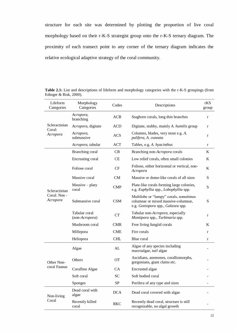
Table 2.1: List and descriptions of lifeform and morphology categories with the r-K-S groupings (from

Edinger & Risk, 2000).

Lifeform

Categories

Morphology

Categories Codes Descriptions

rKS

group

Scleractinian

Coral:

Acropora

Acropora, branching

ACB Staghorn corals, long thin branches r

Acropora, digitate ACD Digitate, stubby, mainly A. humilis group r

Acropora, submassive

ACS Columns, blades, very stout e.g. A. palifera, A. cuneata

r

Acropora, tabular ACT Tables, e.g. A. hyacinthus r

Scleractinian Coral: Non -

Acropora

Branching coral CB Branching non-Acropora corals K

Encrusting coral CE Low relief corals, often small colonies K

Foliose coral CF Foliose, either horizontal or vertical, non-Acropora

K

Massive coral CM Massive or dome-like corals of all sizes S

Massive – platy

coral CMP

Plate-like corals forming large colonies,

e.g. Euphyllia spp., Lobophyllia spp. S

Submassive coral CSM Multilobe or “lumpy” corals, sometimes

columnar or mixed massive-columnar,

e.g. Goniopora spp., Galaxea spp.

S

Tabular coral

(non-Acropora) CT

Tabular non-Acropora, especially

Montipora spp., Turbinaria spp. r

Mushroom coral CMR Free living fungiid corals K

Millepora CME Fire corals r

Heliopora CHL Blue coral r

Other Non-coral Faunas

Algae AL Algae of any species including

macroalgae, turf algae -

Others OT Ascidians, anemones, coralliomorphs, gorgonians, giant clams etc.

-

Coralline Algae CA Encrusted algae -

Soft coral SC Soft bodied coral -

Sponges SP Porifera of any type and sizes -

Non-living Coral

Dead coral with algae

DCA Dead coral covered with algae -

Recently killed

coral RKC

Recently dead coral, structure is still

recognizable, no algal growth -

23

Lifeform

Categories

Morphology

Categories Codes Descriptions

rKS

group

Abiotic

Rock RC Rock of all sizes -

Sand SD Coarse sediment grain, settles to the

bottom quickly if stirred -

Silt SI Fine sediment grain, forms cloud if stirred

-

2.3 Laboratory work

2.3.1 Examination of stomach contents

In the laboratory, stomach contents of 54 fish species were examined using the

volumetric method according to Hyslop (1980). The dietary composition was expressed

in percentage volume of food items averaged according to species. The dietary

composition of fish was used to assign them into or to the closest trophic guild that

would be later used to calculate the trophic fractionation correction for stable isotopic

analysis (see below). Based on its diet, each fish was assigned to one out of five feeding

guilds, namely, ‘Herbivores’ (species that feed largely on plant material including

phytoplankton), ‘Omnivores’ (species that feed on a mixture of plant materials and

animals), ‘Invertivores’ (species that feed entirely on invertebrates), ‘Carnivores’

(species that feed on mixture of fish and invertebrates) and ‘Piscivores’ (species that

feed largely on fish). Fish were assigned to their feeding guild based on the results

obtained from the principal component analysis of the stomach content data. For 23

other fish species with empty stomachs, they were assigned into the respective feeding

guilds based on published information.

2.3.2 Sample preparation for isotopic analysis

Of the total of 97 species sampled, 77 of the most common species were used

for the stable isotopic analysis. Fish tissue samples were dissected from the white

muscles below the dorsal fin. The tissue samples were then washed copiously with

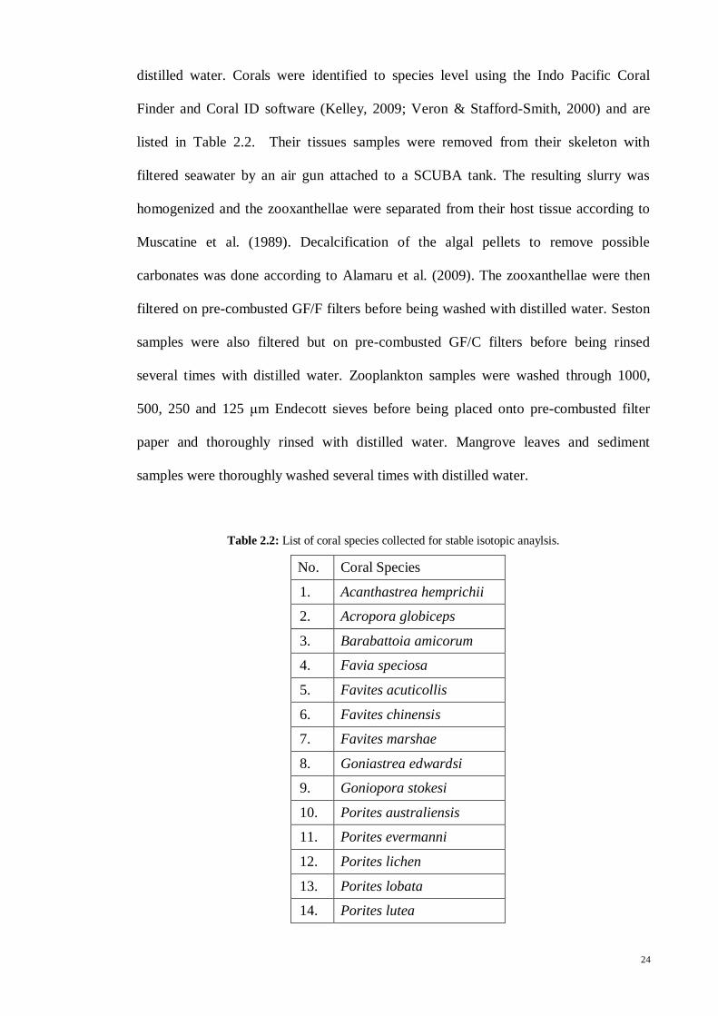
24

distilled water. Corals were identified to species level using the Indo Pacific Coral

Finder and Coral ID software (Kelley, 2009; Veron & Stafford-Smith, 2000) and are

listed in Table 2.2. Their tissues samples were removed from their skeleton with

filtered seawater by an air gun attached to a SCUBA tank. The resulting slurry was

homogenized and the zooxanthellae were separated from their host tissue according to

Muscatine et al. (1989). Decalcification of the algal pellets to remove possible

carbonates was done according to Alamaru et al. (2009). The zooxanthellae were then

filtered on pre-combusted GF/F filters before being washed with distilled water. Seston

samples were also filtered but on pre-combusted GF/C filters before being rinsed

several times with distilled water. Zooplankton samples were washed through 1000,

500, 250 and 125 μm Endecott sieves before being placed onto pre-combusted filter

paper and thoroughly rinsed with distilled water. Mangrove leaves and sediment

samples were thoroughly washed several times with distilled water.

Table 2.2: List of coral species collected for stable isotopic anaylsis.

No. Coral Species

1. Acanthastrea hemprichii

2. Acropora globiceps

3. Barabattoia amicorum

4. Favia speciosa

5. Favites acuticollis

6. Favites chinensis

7. Favites marshae

8. Goniastrea edwardsi

9. Goniopora stokesi

10. Porites australiensis

11. Porites evermanni

12. Porites lichen

13. Porites lobata

14. Porites lutea

25

All processed samples were then dried in the oven at 60°C for 5 days, except

seston and zooxanthellae samples for two days before they were cooled and kept in a

dessicator. All samples were sent to the Marine Biological Laboratory (MBL), Woods

Hole, USA, for dual 13

C and 15

N stable isotopic analysis. The sediment samples were

acid treated to remove particulate inorganic carbonates, whose presence was possible

given the limestone karst. The pulverised dried samples were combusted to N2 and CO2

gases by Europa ANCA-SL elemental analyser. The isotopic carbon and nitrogen ratios

were determined by gas chromatograph system attached to a continuous – flow Europa

20-20 mass spectrometer. Results were expressed in standard δ notation, and the values

were determined based on the following equations:

δ13

C, ‰ = [(13

C/12

C) sample / (13

C/12

C) standard, PDB − 1] × 1000

δ15

N, ‰ = [(15

N/14

N) sample / (15

N/14

N) standard, air − 1] × 1000

Peedee Belemnite (PDB) and N2 in air were used as the standard reference materials for

carbon and nitrogen in stable isotope analysis respectively. The analytical precision was

± 0.1‰ for both δ13

C and δ15

N.

2.4 Data analysis

2.4.1 Physical attributes of seawater and life forms cover

The physical attributes of seawater were tested for differences according to

zones with permutation ANOVA test followed by post hoc t-test whenever significant

difference was detected. Likewise, the same tests were used to detect significant

difference of life forms cover of coral community structure according to sites. These test

analyses were done using the open access R software version 2.15.1.

26

2.4.2 Fish species cluster analysis

Due to the limitation of the catch from gill nets and “bubu”, the species diversity

was likely to be under-estimated. Therefore, species lists from the recent literature were

included in the present study to determine the distribution and range of the fish species

found (Chong, 2005). The locations of sampled fish species from literature were

compared with the zones in the present study. They were then placed into the nearest

possible zones accordingly. Percent disagreement was used to compare the dissimilarity

between sites. Complete linkage percent disagreement cluster analysis was performed

using presence and absence data. A simple dendrogram was constructed to provide a

measure of dissimilarity between sites and habitats. The statistical analysis was

computed using Statistica 8.0 Software.

2.4.3 Habitat complexity and mortality index

The coral reef habitat complexity of each site was estimated as morphology

diversity, which was determined using the Shannon – Wiener diversity index, mH’ as

given below:-

mH’ = - Σ ((pi) (ln pi)),

where pi is the proportion of corals belonging to ith category of morphology (Roberts &

Ormond, 1987). The Shannon – Wiener diversity index was calculated for all of the

morphology categories, where the index near 0 indicates low complexity. Reef

condition was determined by the percentage of live coral cover over the total cover of

all lifeform categories. Mortality index, M was calculated as a proportion of standing

dead coral cover to the total cover of both dead and live corals, where

M = dead coral/(live corals + dead corals) (Gomez, Alino, Yap, & Licuanan,

1994).

27

The closer the index to 0 the more live coral is present in a particular site. The overall

coral cover and indices for the northeast Langkawi were calculated by pooling the data

of all transects over the four sites.

2.4.4 Stomach content and Stable Isotope Analysis in R (SIAR)

Principal component analysis (PCA) was performed on the fish’s dietary

composition from the stomach content analysis. All dietary composition data were

arcsine transformed prior to computing PCA and the result was illustrated in a 2-

dimensional biplot diagram. A simple food web design based on the feeding guilds (Fig.

2.4) was then constructed to determine the trophic fractionation of carbon (∆13

C) and

nitrogen (∆15

N) where ∆ denotes the change in isotope ratio between diet and consumer.

∆13

C and ∆15

N were calculated by adding the trophic shifts values with proportions of

type of food consumed along the path from primary producers to each consumer (Reid

et al. 2008). The trophic shift values between trophic levels were then averaged based

on McCutchan et al. (2003)’s summarised analyses of protein content values and

consumer’s tissue muscles. The calculated ∆13

C and ∆15

N values were incorporated into

the consumers’ isotopic signatures as corrections for trophic fractionation prior to

computing the Stable Isotope Analysis in R (SIAR).

The differences in δ13

C and δ15

N isotopes and C/N ratio were tested according to

two factors, feeding guilds and habitat zones. Both factors were tested separately using

the non-parametric Kruskal-Wallis test followed by a post hoc pairwise Mann-Whitney

analysis, whenever significance was detected. All statistical analyses were done using R

version 2.15.1.

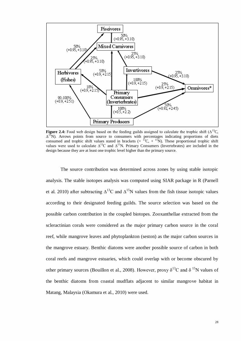
28

Figure 2.4: Food web design based on the feeding guilds assigned to calculate the trophic shift (∆13C,

∆15N). Arrows points from source to consumers with percentages indicating proportions of diets

consumed and trophic shift values stated in brackets (+ 13C, + 15N). These proportional trophic shift

values were used to calculate ∆13C and ∆15N. Primary Consumers (Invertebrates) are included in the

design because they are at least one trophic level higher than the primary source.

The source contribution was determined across zones by using stable isotopic

analysis. The stable isotopes analysis was computed using SIAR package in R (Parnell

et al. 2010) after subtracting ∆13

C and ∆15

N values from the fish tissue isotopic values

according to their designated feeding guilds. The source selection was based on the

possible carbon contribution in the coupled biotopes. Zooxanthellae extracted from the

scleractinian corals were considered as the major primary carbon source in the coral

reef, while mangrove leaves and phytoplankton (seston) as the major carbon sources in

the mangrove estuary. Benthic diatoms were another possible source of carbon in both

coral reefs and mangrove estuaries, which could overlap with or become obscured by

other primary sources (Bouillon et al., 2008). However, proxy δ13

C and δ 15

N values of

the benthic diatoms from coastal mudflats adjacent to similar mangrove habitat in

Matang, Malaysia (Okamura et al., 2010) were used.

29

3.0 RESULTS

3.1 Seawater physical attributes of biotopes

The measurements of all physical attributes in each zone are presented in Table

3.1 and Table 3.2. Salinity and pH showed a decreasing pattern from Coral zone (31.96

± 0.16 SE ‰ and 8.05 ± 0.15 SE respectively) towards the Up zone (29.99 ± 0.46 ‰

and 7.54 ± 0.10). Temperature was highest in the Coral zone, with 30.57 °C and

decreased towards the Mg-C zone, 29.74 °C and the Mg zone 29.84 °C. The lowest

temperature was recorded in the Up zone at 29.27 °C, approximately just 1 °C lower

than at the Coral zone. The opposite pattern was observed for TDS in which 31.30 was

measured in the Coral zone and decreased to 29.29 in the Mg zone before an increment

of just 0.24 in the Up zone. DO measurements recorded an inconsistent pattern from the

Coral zone towards the Up zone with readings of 5.52, 4.68, 5.33 and 4.36 mg/L,

respectively. Most physical parameters showed relatively consistent measurements

except for Turbidity and ORP, which had high SE values. The least turbid zone was in

the Up zone with just 9.71 ± 1.84 NTU, followed by Coral, 25.87 ± 7.70 NTU and Mg,

26.20 ± 5.87 NTU. The Mg-C zone measured as the most turbid zone with a reading of

54.05 ± 34.48 NTU. Despite the high SE of the ORP reading in the coral reef, the mean

of ORP across all zones remained within the range of between 349.33 to 409.92 mV. In

general, all physical attributes recorded higher values in the coral reef and lower values

in the mangrove creeks, except for ORP.

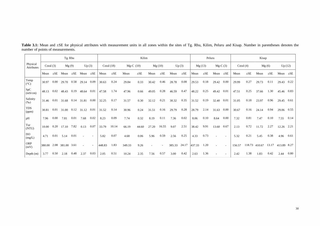
30

Table 3.1: Mean and ±SE for physical attributes with measurement units in all zones within the sites of Tg. Rhu, Kilim, Peluru and Kisap. Number in parentheses denotes the

number of points of measurements.

Physical

Attributes

Tg. Rhu Kilim Peluru Kisap

Coral (3) Mg (9) Up (3) Coral (18) Mg-C (10) Mg (10) Up (3) Mg (13) Mg-C (3) Coral (4) Mg (6) Up (12)

Mean ±SE Mean ±SE Mean ±SE Mean ±SE Mean ±SE Mean ±SE Mean ±SE Mean ±SE Mean ±SE Mean ±SE Mean ±SE Mean ±SE

Temp

(°C) 30.97 0.00 29.70 0.58 29.14 0.09 30.63 0.24 29.84 0.33 30.42 0.46 28.78 0.08 29.53 0.18 29.42 0.00 29.99 0.27 29.73 0.11 29.43 0.22

SpC

(mS/cm) 48.13 0.02 48.43 0.19 48.64 0.01 47.58 1.74 47.96 0.66 49.05 0.28 46.59 0.47 48.22 0.25 49.42 0.01 47.51 0.25 37.66 1.30 45.46 0.83

Salinity (‰)

31.46 0.01 31.68 0.14 31.81 0.00 32.25 0.17 31.57 0.30 32.12 0.21 30.32 0.35 31.52 0.19 32.40 0.01 31.05 0.18 23.97 0.96 29.45 0.61

TDS

(ppm) 30.81 0.01 31.00 0.12 31.12 0.01 31.52 0.14 30.96 0.24 31.51 0.16 29.79 0.28 28.79 2.14 31.63 0.00 30.67 0.16 24.14 0.94 29.06 0.55

pH 7.96 0.00 7.81 0.01 7.68 0.02 8.23 0.09 7.74 0.32 8.19 0.11 7.36 0.02 8.06 0.10 8.64 0.00 7.32 0.81 7.47 0.10 7.55 0.14

Tur (NTU)

10.00 0.20 17.10 7.82 0.13 0.07 33.79 10.14 66.19 44.60 27.20 16.55 9.07 2.51 38.42 9.91 13.60 0.67 2.13 0.72 11.72 2.27 12.26 2.21

DO

(mg/L) 4.71 0.01 5.14 0.01 - - 5.82 0.07 4.68 0.06 5.96 0.59 2.56 0.25 4.33 0.73 - - 5.32 0.21 5.45 0.38 4.96 0.61

ORP

(mV) 380.00 2.08 381.00 3.61 - - 448.83 1.83 349.33 9.26 - - 385.33 24.17 437.33 1.20 - - 156.57 118.73 410.67 13.17 413.89 8.27

Depth (m) 3.77 0.50 2.18 0.48 2.37 0.03 2.05 0.51 10.24 2.35 7.56 0.57 3.00 0.42 2.63 1.36 - - 2.42 1.38 1.83 0.42 2.44 0.80

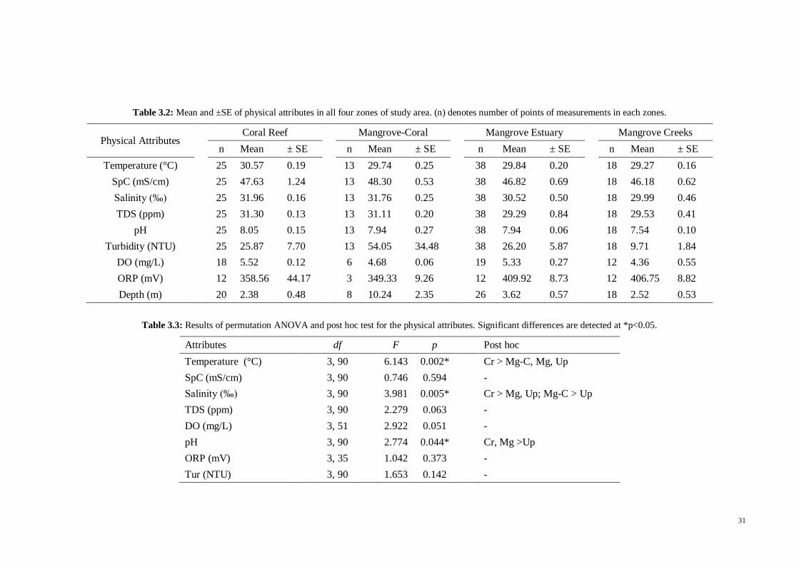
31

Table 3.2: Mean and ±SE of physical attributes in all four zones of study area. (n) denotes number of points of measurements in each zones.

Physical Attributes Coral Reef Mangrove-Coral Mangrove Estuary Mangrove Creeks

n Mean ± SE n Mean ± SE n Mean ± SE n Mean ± SE

Temperature (°C) 25 30.57 0.19 13 29.74 0.25 38 29.84 0.20 18 29.27 0.16

SpC (mS/cm) 25 47.63 1.24 13 48.30 0.53 38 46.82 0.69 18 46.18 0.62

Salinity (‰) 25 31.96 0.16 13 31.76 0.25 38 30.52 0.50 18 29.99 0.46

TDS (ppm) 25 31.30 0.13 13 31.11 0.20 38 29.29 0.84 18 29.53 0.41

pH 25 8.05 0.15 13 7.94 0.27 38 7.94 0.06 18 7.54 0.10

Turbidity (NTU) 25 25.87 7.70 13 54.05 34.48 38 26.20 5.87 18 9.71 1.84

DO (mg/L) 18 5.52 0.12 6 4.68 0.06 19 5.33 0.27 12 4.36 0.55

ORP (mV) 12 358.56 44.17 3 349.33 9.26 12 409.92 8.73 12 406.75 8.82

Depth (m) 20 2.38 0.48 8 10.24 2.35 26 3.62 0.57 18 2.52 0.53

Table 3.3: Results of permutation ANOVA and post hoc test for the physical attributes. Significant differences are detected at *p<0.05.

Attributes df F p Post hoc

Temperature (°C) 3, 90 6.143 0.002* Cr > Mg-C, Mg, Up

SpC (mS/cm) 3, 90 0.746 0.594 -

Salinity (‰) 3, 90 3.981 0.005* Cr > Mg, Up; Mg-C > Up

TDS (ppm) 3, 90 2.279 0.063 -

DO (mg/L) 3, 51 2.922 0.051 -

pH 3, 90 2.774 0.044* Cr, Mg >Up

ORP (mV) 3, 35 1.042 0.373 -

Tur (NTU) 3, 90 1.653 0.142 -

32

Permutation ANOVA revealed that the differences in physical attributes among

zones were all insignificant except for temperature, salinity and pH (p < 0.05). Post-hoc

t-test detected that the Coral zone was significantly different from all the other zones

with respect to temperature. In terms of salinity, significant differences were detected

between Coral and Mg, Coral and Up zones as well as between mixed Mg-C and Up

zones. As for pH, Coral and Mg zones were found to have significantly higher values

than the Up zone (Table 3.3). Although only these three physical attributes were

significantly different among zones, their mean differences were less than 2 units.

3.2 Fish species diversity and similarity

In the present study, a total of 97 species of fish from 38 families were sampled.

The inclusion from a previous study from Chong et al. (2005) adds up to a total number

of 147 fish species from 52 families for the whole northeast of Langkawi (see Appendix

I). In Tg. Rhu, the Coral, Mg-C and Mg zones had 18, 36 and 10 species respectively.

Kilim, where the main river system lies, had a total of 35, 47, 37 and 19 species in the

Coral, Mg-C, Mg and Up zones respectively. Peluru Straits on the other hand, had only

16 species in the Mg-C zone and 40 species in the Mg zone. Another site of major river

system, Kisap, had 22 species in its Coral zone and 29 in the mixed Mg-C zone station.

The Mg station in Kisap however, had only 10 species while the Up zone had an

additional 9 more species. Percent disagreement matrix and dendogram were then

constructed below (Table 3.4 and Fig. 3.1). This initial analysis was done to compare

the fish species composition between zones prior to further analysis.

33

Table 3.4: Percent Disagreement Matrix calculated using Statistica 8.0 Software. TC = Tg. Rhu coral, TMU = Tg. Rhu

upstream mangrove, KMU = Kilim upstream mangrove, SMC = Kisap mangrove-coral, SMU = Kisap upstream

mangrove, PMC = Peluru Straits mangrove-coral, SC = Kisap coral, KC = Kilim coral, TM = Tg. Rhu mangrove, KM =

Kilim mangrove, PM = Peluru Straits mangrove, SM = Kisap mangrove, KMC = Kilim mangrove-coral.

Percent disagreement (CA.sta)

TC TM TMU KC KMC KM KMU PMC PM SC SM SMC SMU

TC 0.00 0.31 0.18 0.27 0.39 0.31 0.22 0.20 0.31 0.23 0.27 0.16 0.21

TM 0.31 0.00 0.27 0.35 0.41 0.35 0.28 0.33 0.39 0.31 0.29 0.27 0.28

TMU 0.18 0.27 0.00 0.28 0.32 0.27 0.13 0.15 0.26 0.20 0.22 0.14 0.16

KC 0.27 0.35 0.28 0.00 0.41 0.37 0.29 0.32 0.40 0.28 0.38 0.29 0.29

KMC 0.39 0.41 0.32 0.41 0.00 0.31 0.30 0.31 0.46 0.39 0.46 0.35 0.34

KM 0.31 0.35 0.27 0.37 0.31 0.00 0.26 0.27 0.31 0.35 0.30 0.27 0.22

KMU 0.22 0.28 0.13 0.29 0.30 0.26 0.00 0.18 0.27 0.22 0.22 0.14 0.16

PMC 0.20 0.33 0.15 0.32 0.31 0.27 0.18 0.00 0.34 0.23 0.29 0.15 0.18

PM 0.31 0.39 0.26 0.40 0.46 0.31 0.27 0.34 0.00 0.31 0.25 0.26 0.24

SC 0.23 0.31 0.20 0.28 0.39 0.35 0.22 0.23 0.31 0.00 0.29 0.20 0.24

SM 0.27 0.29 0.22 0.38 0.46 0.30 0.22 0.29 0.25 0.29 0.00 0.18 0.19

SMC 0.16 0.27 0.14 0.29 0.35 0.27 0.14 0.15 0.26 0.20 0.18 0.00 0.14

SMU 0.21 0.28 0.16 0.29 0.34 0.22 0.16 0.18 0.24 0.24 0.19 0.14 0.00

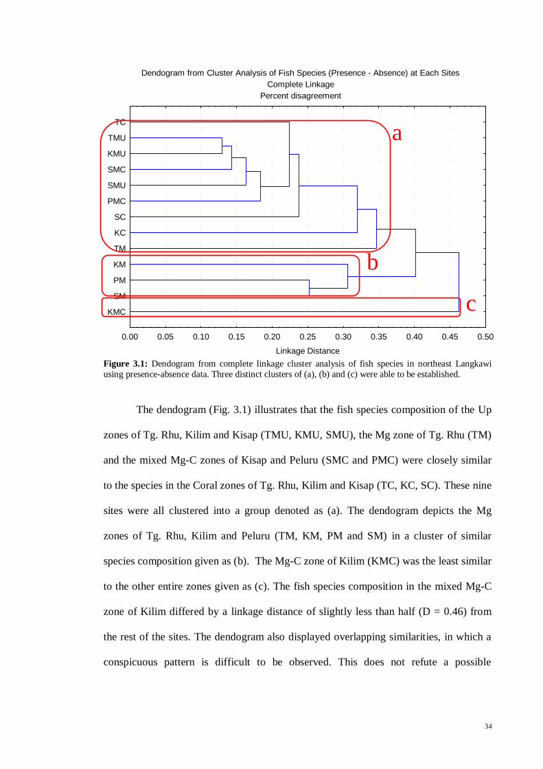
34

Dendogram from Cluster Analysis of Fish Species (Presence - Absence) at Each Sites

Complete Linkage

Percent disagreement

0.00 0.05 0.10 0.15 0.20 0.25 0.30 0.35 0.40 0.45 0.50

Linkage Distance

KMC

SM

PM

KM

TM

KC

SC

PMC

SMU

SMC

KMU

TMU

TC

Figure 3.1: Dendogram from complete linkage cluster analysis of fish species in northeast Langkawi

using presence-absence data. Three distinct clusters of (a), (b) and (c) were able to be established.

The dendogram (Fig. 3.1) illustrates that the fish species composition of the Up

zones of Tg. Rhu, Kilim and Kisap (TMU, KMU, SMU), the Mg zone of Tg. Rhu (TM)

and the mixed Mg-C zones of Kisap and Peluru (SMC and PMC) were closely similar

to the species in the Coral zones of Tg. Rhu, Kilim and Kisap (TC, KC, SC). These nine

sites were all clustered into a group denoted as (a). The dendogram depicts the Mg

zones of Tg. Rhu, Kilim and Peluru (TM, KM, PM and SM) in a cluster of similar

species composition given as (b). The Mg-C zone of Kilim (KMC) was the least similar

to the other entire zones given as (c). The fish species composition in the mixed Mg-C

zone of Kilim differed by a linkage distance of slightly less than half (D = 0.46) from

the rest of the sites. The dendogram also displayed overlapping similarities, in which a

conspicuous pattern is difficult to be observed. This does not refute a possible

a

c

b

35

connection, however a clear conclusion could not be drawn. Thus, in order to determine

if a conspicuous connection does exist, Table 3.5 and Fig. 3.2 were constructed.

Table 3.5 below displays a checklist of fish species which has been pooled into

the four given zones namely Coral, Mg-C, Mg and Up, regardless of sites. The lowest

number of fish species was in the Up zone with only 35 species. The fish diversity in

the northeast Langkawi was highest in the Mg zone with 90 species as compared to the

Coral zone, which harboured only 59 species. Since the mangrove biotope comprised

both Mg and Up zones, the species that occurs in both zones were counted only once,

making up the total number of 98 species present in the mangrove biotope. Finally, 60

species were found in the mixed Mg-C zone.

Table 3.5: List of fish species in northeast Langkawi, separated in to four major zones; coral (Coral),

mangrove-coral (Mg-C), mangrove (Mg) and mangrove creeks (Up). “*” denotes species that were only

found in literature but not in present study. 1 = present, 0 = absent

Family Species Coral Mg-C Mg Up

Ambassidae Ambassis nalua 0 0 1 1

Apogonidae Apogon hyalosoma 0 1 0 1

Ariidae Arius caelatus 0 1* 0 1*

Arius tenuispinis 0 0 0 1*

Arius venosus 0 1* 0 0

Hexanematichtys sagor 0 0 1 1

Osteogeneiosus militaris 0 0 1* 0

Batrachoididae Allenbatrachus grunniens 0 1* 0 0

Belonidae Strongylura strongylura 0 0 1 0

Tylosurus crocodilus

crocodilus

0 0 1 1

Caesionidae Caesio cunning 1 1 1 0

Callionymidae Callionymus sagitta 0 0 1* 0

Carangidae Alectis indicus 0 1* 0 0

Alepes djedaba 0 0 1 0

Alepes kleinii 1 0 0 0

Atule mate 1 0 0 0

Carangoides equula 1* 0 1* 0

Carangoides oblongus 0 0 1 0

Carangoides praeustus 1 1 1 1

Caranx ignobilis 0 1 1 1*

Caranx sexfasciatus 1 1 1 0

Scomberoides

commersonnianus

1 1 1 1

Scomberoides lysan 0 1 1 1

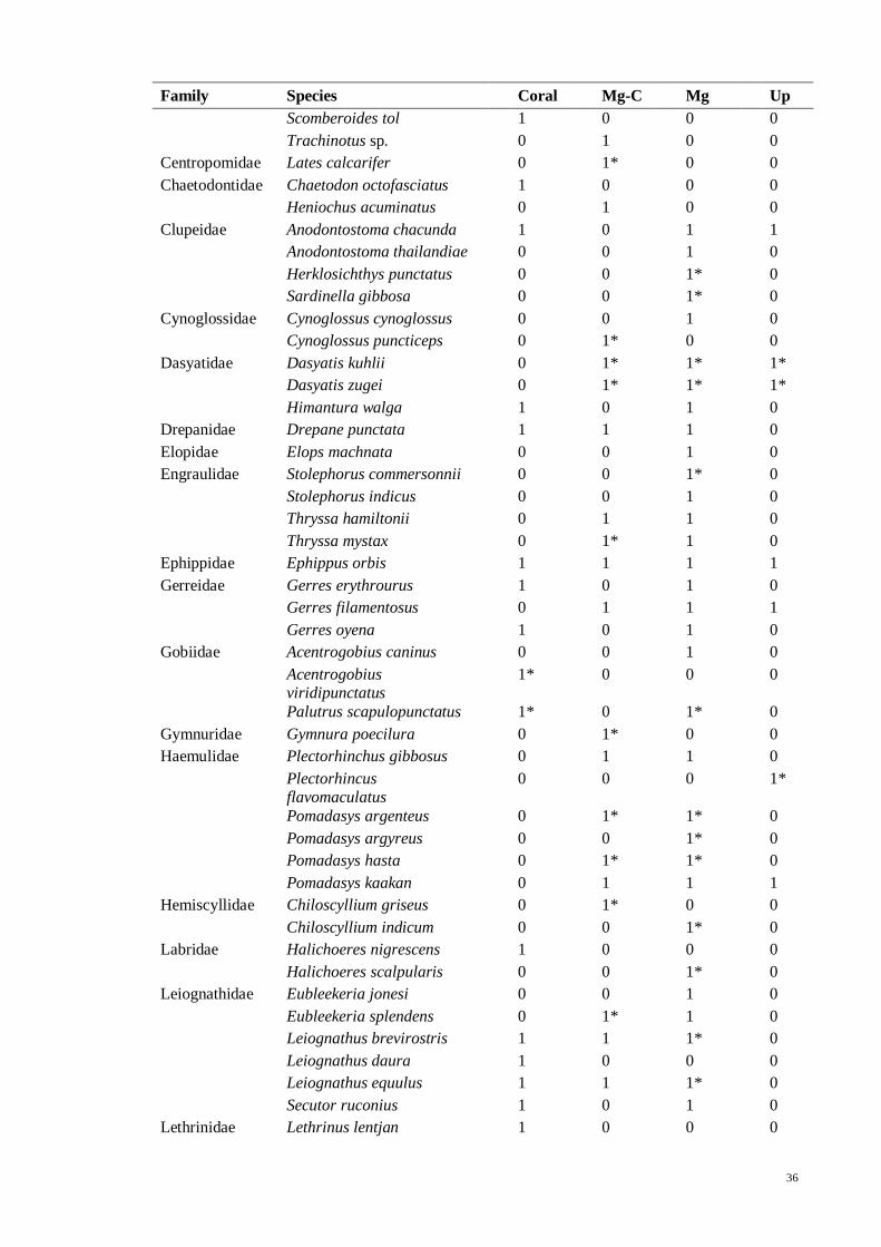
36

Family Species Coral Mg-C Mg Up

Scomberoides tol 1 0 0 0

Trachinotus sp. 0 1 0 0

Centropomidae Lates calcarifer 0 1* 0 0

Chaetodontidae Chaetodon octofasciatus 1 0 0 0

Heniochus acuminatus 0 1 0 0

Clupeidae Anodontostoma chacunda 1 0 1 1

Anodontostoma thailandiae 0 0 1 0

Herklosichthys punctatus 0 0 1* 0

Sardinella gibbosa 0 0 1* 0

Cynoglossidae Cynoglossus cynoglossus 0 0 1 0

Cynoglossus puncticeps 0 1* 0 0

Dasyatidae Dasyatis kuhlii 0 1* 1* 1*

Dasyatis zugei 0 1* 1* 1*

Himantura walga 1 0 1 0

Drepanidae Drepane punctata 1 1 1 0

Elopidae Elops machnata 0 0 1 0

Engraulidae Stolephorus commersonnii 0 0 1* 0

Stolephorus indicus 0 0 1 0

Thryssa hamiltonii 0 1 1 0

Thryssa mystax 0 1* 1 0

Ephippidae Ephippus orbis 1 1 1 1

Gerreidae Gerres erythrourus 1 0 1 0

Gerres filamentosus 0 1 1 1

Gerres oyena 1 0 1 0

Gobiidae Acentrogobius caninus 0 0 1 0

Acentrogobius viridipunctatus

1* 0 0 0

Palutrus scapulopunctatus 1* 0 1* 0

Gymnuridae Gymnura poecilura 0 1* 0 0

Haemulidae Plectorhinchus gibbosus 0 1 1 0

Plectorhincus flavomaculatus

0 0 0 1*

Pomadasys argenteus 0 1* 1* 0

Pomadasys argyreus 0 0 1* 0

Pomadasys hasta 0 1* 1* 0

Pomadasys kaakan 0 1 1 1

Hemiscyllidae Chiloscyllium griseus 0 1* 0 0

Chiloscyllium indicum 0 0 1* 0

Labridae Halichoeres nigrescens 1 0 0 0

Halichoeres scalpularis 0 0 1* 0

Leiognathidae Eubleekeria jonesi 0 0 1 0

Eubleekeria splendens 0 1* 1 0

Leiognathus brevirostris 1 1 1* 0

Leiognathus daura 1 0 0 0

Leiognathus equulus 1 1 1* 0

Secutor ruconius 1 0 1 0

Lethrinidae Lethrinus lentjan 1 0 0 0

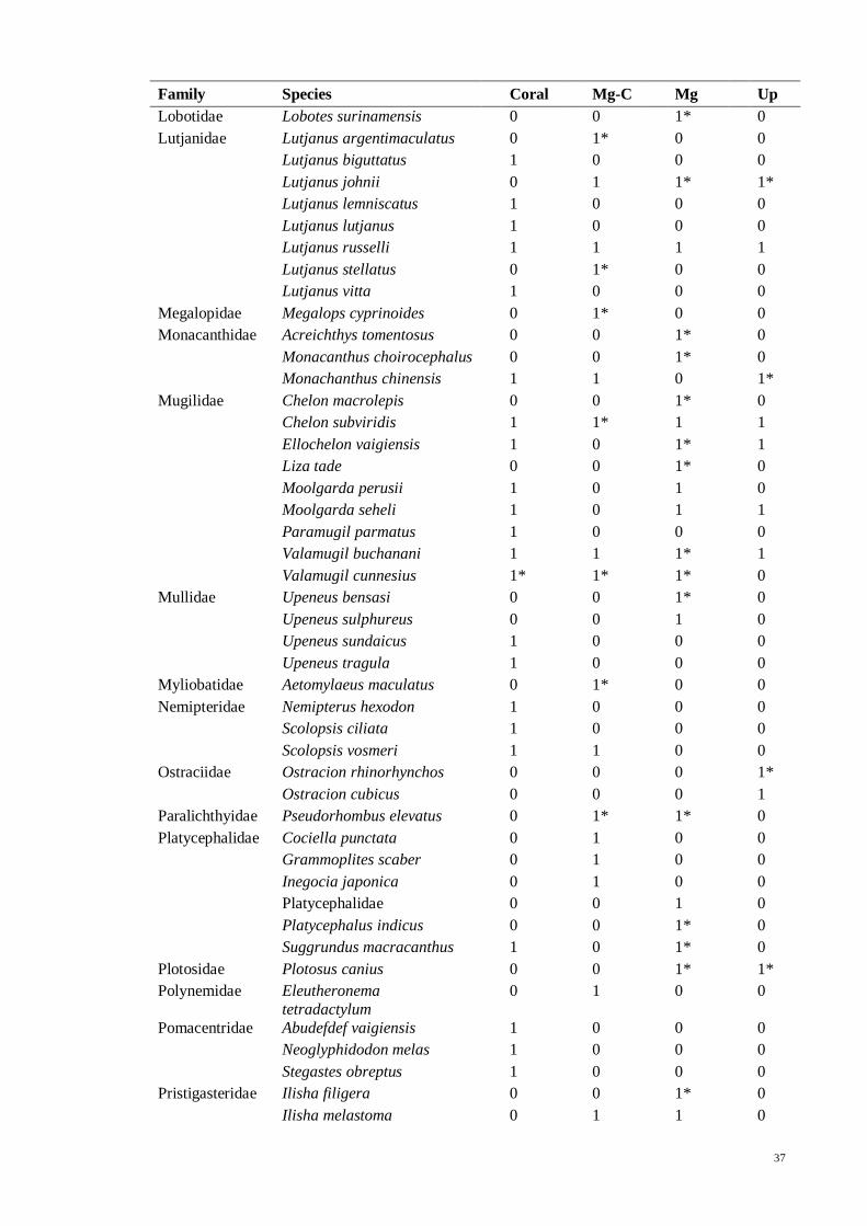
37

Family Species Coral Mg-C Mg Up

Lobotidae Lobotes surinamensis 0 0 1* 0

Lutjanidae Lutjanus argentimaculatus 0 1* 0 0

Lutjanus biguttatus 1 0 0 0

Lutjanus johnii 0 1 1* 1*

Lutjanus lemniscatus 1 0 0 0

Lutjanus lutjanus 1 0 0 0

Lutjanus russelli 1 1 1 1

Lutjanus stellatus 0 1* 0 0

Lutjanus vitta 1 0 0 0

Megalopidae Megalops cyprinoides 0 1* 0 0

Monacanthidae Acreichthys tomentosus 0 0 1* 0

Monacanthus choirocephalus 0 0 1* 0

Monachanthus chinensis 1 1 0 1*

Mugilidae Chelon macrolepis 0 0 1* 0

Chelon subviridis 1 1* 1 1

Ellochelon vaigiensis 1 0 1* 1

Liza tade 0 0 1* 0

Moolgarda perusii 1 0 1 0

Moolgarda seheli 1 0 1 1

Paramugil parmatus 1 0 0 0

Valamugil buchanani 1 1 1* 1

Valamugil cunnesius 1* 1* 1* 0

Mullidae Upeneus bensasi 0 0 1* 0

Upeneus sulphureus 0 0 1 0

Upeneus sundaicus 1 0 0 0

Upeneus tragula 1 0 0 0

Myliobatidae Aetomylaeus maculatus 0 1* 0 0

Nemipteridae Nemipterus hexodon 1 0 0 0

Scolopsis ciliata 1 0 0 0

Scolopsis vosmeri 1 1 0 0

Ostraciidae Ostracion rhinorhynchos 0 0 0 1*

Ostracion cubicus 0 0 0 1

Paralichthyidae Pseudorhombus elevatus 0 1* 1* 0

Platycephalidae Cociella punctata 0 1 0 0

Grammoplites scaber 0 1 0 0

Inegocia japonica 0 1 0 0

Platycephalidae 0 0 1 0

Platycephalus indicus 0 0 1* 0

Suggrundus macracanthus 1 0 1* 0

Plotosidae Plotosus canius 0 0 1* 1*

Polynemidae Eleutheronema

tetradactylum

0 1 0 0

Pomacentridae Abudefdef vaigiensis 1 0 0 0

Neoglyphidodon melas 1 0 0 0

Stegastes obreptus 1 0 0 0

Pristigasteridae Ilisha filigera 0 0 1* 0

Ilisha melastoma 0 1 1 0

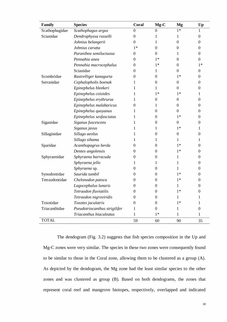
38

Family Species Coral Mg-C Mg Up

Scathophagidae Scathophagus argus 0 0 1* 1

Scianidae Dendrophyssa russelli 0 1 1 0

Johnius belangerii 0 1 0 0

Johnius carutta 1* 0 0 0

Paranibea semiluctuosa 0 0 1 0

Pennahia anea 0 1* 0 0

Pennahia macrocephalus 0 1* 0 1*

Scianidae 0 1 0 0

Scombridae Rastrelliger kanagurta 0 0 1* 0

Serranidae Cephalopholis boenak 1 0 0 0

Epinephelus bleekeri 1 1 0 0

Epinephelus coioides 1 1* 1* 1

Epinephelus erythrurus 1 0 0 0

Epinephelus malabaricus 0 1 0 0

Epinephelus quoyanus 1 0 0 0

Epinephelus sexfasciatus 1 0 1* 0

Siganidae Siganus fuscescens 1 0 0 0

Siganus javus 1 1 1* 1

Sillaginidae Sillago aeolus 1 0 0 0

Sillago sihama 1 1 1 1

Sparidae Acanthopagrus berda 0 0 1* 0

Dentex angolensis 0 0 1* 0

Sphyraenidae Sphyraena barracuda 0 0 1 0

Sphyraena jello 1 1 1 0

Sphyraena sp. 0 0 1 0

Synodontidae Saurida tumbil 0 0 1* 0

Tetraodontidae Chelonodon patoca 0 0 1* 0

Lagocephalus lunaris 0 0 1 0

Tetraodon fluviatilis 0 0 1* 0

Tetraodon nigroviridis 0 0 1 1

Toxotidae Toxotes jaculatrix 0 0 1* 1

Triacanthidae Pseudotriacanthus strigilifer 1 0 1 0

Triacanthus biaculeatus 1 1* 1 1

TOTAL 59 60 90 35

The dendogram (Fig. 3.2) suggests that fish species composition in the Up and

Mg-C zones were very similar. The species in these two zones were consequently found

to be similar to those in the Coral zone, allowing them to be clustered as a group (A).

As depicted by the dendogram, the Mg zone had the least similar species to the other

zones and was clustered as group (B). Based on both dendograms, the zones that

represent coral reef and mangrove biotopes, respectively, overlapped and indicated

39

some degree of similarity. This implies that there are common fishes in both biotopes,

and which are identified and listed in Table 3.6, illustrating the connectivity between

coral and mangrove biotopes.

Dendogram for Cluster Analysis of Four Zones of Habitats

Complete Linkage

Percent disagreement

0.30 0.35 0.40 0.45 0.50 0.55 0.60 0.65

Linkage Distance

Mangrove

Upper

Mg-C

Coral

Figure 3.2: Dendogram from complete linkage percent disagreement cluster analysis of fish species in northeast Langkawi using presence-absence data.

Table 3.6: List of common species to both coral reefs and mangroves biotopes in northeast Langkawi.

Fish species that are considered common are the species found in the coral reefs (“Coral”) and in

mangroves, which includes mangrove creeks (“Mangrove” + “Up”). Mangrove-coral zone (“Mg-C”) is

considered a mixed zone, where the boundary of coral and mangrove is unable to be distinguished. “0”

denotes species absent; “1” denotes species present whereas “1*” denotes species that are present in

previous studies (Chong et al, 2005).

Family Species Coral Mg-C Mg Up

Caesionidae Caesio cunning 1 1 1 0

Carangidae Carangoides equula 1* 0 1* 0

Carangidae Carangoides praeustus 1 1 1 1

Carangidae Caranx sexfasciatus 1 1 1 0

Carangidae Scomberoides commersonnianus 1 1 1 1

Clupeidae Anodontostoma chacunda 1 0 1 1

Dasyatidae Himantura walga 1 0 1 0

Drepanidae Drepane punctate 1 1 1 0

Ephippidae Ephippus orbis 1 1 1 1

A

B

40

Family Species Coral Mg-C Mg Up

Gerreidae Gerres erythrourus 1 0 1 0

Gerreidae Gerres oyena 1 0 1 0

Gobiidae Palutrus scapulopunctatus 1* 0 1* 0

Leiognathidae Leiognathus brevirostris 1 1 1* 0

Leiognathidae Leiognathus equulus 1 1 1* 0

Leiognathidae Secutor ruconius 1 0 1 0

Lutjanidae Lutjanus russelli 1 1 1 1

Monachantidae Monachanthus chinensis 1 1 0 1*

Mugilidae Chelon subviridis 1 1* 1 1

Mugilidae Ellochelon vaigiensis 1 0 1* 1

Mugilidae Moolgarda perusii 1 0 1 0

Mugilidae Moolgarda seheli 1 0 1 1

Mugilidae Valamugil buchanani 1 1 1* 1

Mugilidae Valamugil cunnesius 1* 1* 1* 0

Platycephalidae Suggrundus macracanthus 1 0 1* 0

Serranidae Epinephelus coioides 1 1* 1* 1

Serranidae Epinephelus sexfasciatus 1 0 1* 0

Siganidae Siganus javus 1 1 1* 1

Sillaginidae Sillago sihama 1 1 1 1

Sphyraenidae Sphyraena jello 1 1 1 0

Triacanthidae Pseudotriacanthus strigilifer 1 0 1 0

Triacanthidae Triacanthus biaculeatus 1 1* 1 1

TOTAL 31 18 30 14

Table 3.6 lists a total of 31 common species, with 8 represented from previous

studies. Thus, ten of the common fishes Carangoides praeustus, Scomberoides

commersonnianus, Ephippus orbis, Lutjanus russelli, Sillago sihama, Chelon subviridis,

Valamugil buchanani, Epinephelus coioides, Siganus javus and Triacanthus biaculeatus

were found in all four zones with the latter five species from previous studies found in

at least one zone. These 31 species signify that they were widely distributed in all zones.

Fourteen species were found in the mixed Mg-C zones in the present study, none could

be categorized as reef or mangrove dependent.

Table 3.7 displays the total length (TL) of the common species in all four zones,

separated into juveniles and adults based on the one third of maximum length rule

(Dorenbosch et al., 2005; Nagelkerken & van der Velde, 2002). Only Caranx

sexfasciatus and Scomberoides commersonnianus were caught as juvenile in both

biotopes as well as the mixed mangrove-coral zone. In contrast, other species were

41

caught as adult in both of the biotopes, such as Carangoides praestus, Anodontostoma

chachunda, Himantura walga, Ephippus orbis, Gerres oyena, Leiognathus brevirostris,

Chelon subviridis, Moolgarda perusii, Silago sihama, Sphyraena jello,

Pseudotriacanthus strigilifer and Triacanthus biaculaetus. Eight of the common

species, Caesio cunning, Drepane punctata, Gerres erythrourus, Lutjanus ruselli,

Ellochelon vaigiensis, Moolgarda seheli, Epinephelus coiodes and Siganus javus were

caught as a mixture of juveniles and adults in either biotope. Only one species of mullet,

Valamugil buchanani was caught as juvenile in the coral reef and as adult in the

mangrove. Table 3.7 also shows that there were more species at the adult than juvenile

stage in the mangrove and coral reef.

42

Table 3.7: Lengths (mean ± SD) of 23 common fish species in coral reefs (Coral zone only) and mangroves (Mg and Up zones) biotopes including the mixed mangrove coral zone

(Mg-C). Juvenile lengths for respective species were determined with a third of maximum length rule. “*” denotes coastal water species while “^” denotes reef-associated species.

Species

Max

Juvenile

Length

Juvenile Adult

Coral Mg-C Mg Up Coral Mg-C Mg Up

Caesio cunning* 20.00 16.03 ± 0.60 15.90 12.27 ± 0.14 0 0 0 21.80 ± 0.14 0

Carangoides praeustus* 8.30 0 0 0 0 15.00 13.57 ± 0.90 13.58 ± 1.46 14.57 ± 1.79

Caranx sexfasciatus^ 30.00 19.08 ± 1.61 18.40 ± 4.71 17.33 ± 3.59 0 0 0 0 0

Scomberoides commersonnianus^ 30.00 24.80 13.50 17.75 ± 3.52 14.77 ± 1.19 0 0 0 0

Anodontostoma chacunda 7.30 0 0 0 0 15.20 ± 0.66 0 13.15 ± 1.85 12.47 ± 0.71

Himantura walga 15.00 0 0 0 0 17.40 0 17.70 0

Drepane punctata^ 16.70 0 14.50 15.50 0 24.40 ± 8.63 21.18 ± 4.12 29.40 ± 7.50 0

Ephippus orbis^ 8.30 0 0 0 0 16.50 ± 0.71 16.80 ± 0.42 17.50 0

Gerres erythrourus^ 10.00 0 0 9.70 ± 0.28 0 20.60 0 12.75 ± 3.46 0

Gerres oyena^ 10.00 0 0 0 0 15.81 ± 3.31 0 11.30 ± 0.14 0

Leiognathus brevirostris 4.50 0 0 0 0 9.50 10.95 ± 0.35 10.08 ± 1.02 0

Lutjanus russelli^ 16.70 16.57 ± 0.67 15.75 ± 0.49 0 13.00 16.95 ± 0.07 17.50 17.40 0

Chelon subviridis 13.30 0 0 0 0 20.40 0 20.25 ± 4.39 18.60 ± 2.83

Ellochelon vaigiensis^ 21.00 18.00 ± 2.18 0 0 0 27.03 ± 6.38 0 0 28.07 ± 2.83

Moolgarda seheli^ 20.00 19.00 ± 1.41 0 19.05 ± 0.49 16.60 24.39 ± 3.89 0 26.79 ± 3.01 30.50 ± 7.09

Moolgarda perusii^ 8.30 0 0 0 0 20.24 ± 1.65 0 21.08 ± 2.43 0

Valamugil buchanani 30.00 19.10 ± 0.28 17.40 0 0 0 0 0 34.55 ± 2.76

Epinephelus coioides^ 30.00 20.78 ± 2.25 0 0 15.40 0 0 0 33.50 ± 4.24

Siganus javus^ 17.60 16.70 ± 1.13 0 0 10.50 23.20 ± 7.35 21.00 0 0

Sillago sihama^ 10.00 0 0 0 0 15.20 18.27 ± 1.52 17.15 ± 3.97 17.55 ± 4.31

Sphyraena jello^ 30.00 0 0 0 0 46.50 34.90 ± 0.28 33.00 ± 2.12 0

Pseudotriacanthus strigilifer 8.30 0 0 0 0 18.00 0 14.50 0

Triacanthus biaculeatus 10.00 0 0 0 0 18.50 0 11.75 ± 0.07 15.30 ± 3.51

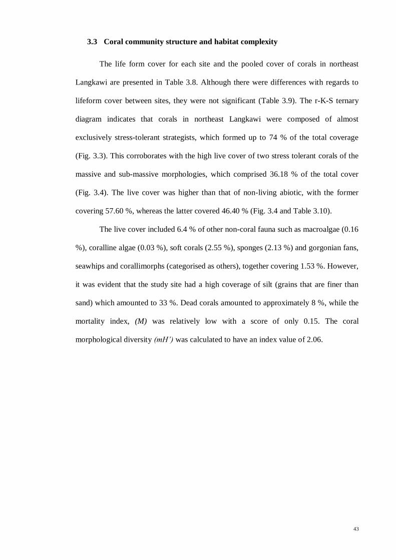
43

3.3 Coral community structure and habitat complexity

The life form cover for each site and the pooled cover of corals in northeast

Langkawi are presented in Table 3.8. Although there were differences with regards to

lifeform cover between sites, they were not significant (Table 3.9). The r-K-S ternary

diagram indicates that corals in northeast Langkawi were composed of almost

exclusively stress-tolerant strategists, which formed up to 74 % of the total coverage

(Fig. 3.3). This corroborates with the high live cover of two stress tolerant corals of the

massive and sub-massive morphologies, which comprised 36.18 % of the total cover

(Fig. 3.4). The live cover was higher than that of non-living abiotic, with the former

covering 57.60 %, whereas the latter covered 46.40 % (Fig. 3.4 and Table 3.10).

The live cover included 6.4 % of other non-coral fauna such as macroalgae (0.16

%), coralline algae (0.03 %), soft corals (2.55 %), sponges (2.13 %) and gorgonian fans,

seawhips and corallimorphs (categorised as others), together covering 1.53 %. However,

it was evident that the study site had a high coverage of silt (grains that are finer than

sand) which amounted to 33 %. Dead corals amounted to approximately 8 %, while the

mortality index, (M) was relatively low with a score of only 0.15. The coral

morphological diversity (mH’) was calculated to have an index value of 2.06.

44

Table 3.8: Percentage cover (mean ± SE) of coral life form categories in four sites – Tg. Rhu, Kilim, Peluru and Kisap. Number in parentheses denotes the number of transects. The

last column represents the percentage cover of the whole of northeast Langkawi.

Lifeform Categories CODES

SITES (%)

Tg Rhu (4) Kilim (9) Peluru (1) Kisap (5) NE Langkawi (19)

Mean ± SE Mean ± SE Mean ± SE Mean ± SE

Live Scleractinian Corals

ACB 0.00 0.00 0.00 0.00 0.00 0.30 0.30 0.08 0.02

ACS 6.13 6.13 0.00 0.00 0.00 1.10 1.10 1.58 0.36

ACT 0.25 0.25 0.00 0.00 0.00 0.00 0.00 0.05 0.01

CE 3.00 1.85 4.61 1.45 14.00 5.70 3.50 5.05 1.16

CF 0.00 0.00 3.67 1.85 0.00 0.20 0.20 1.79 0.41

CM 5.00 1.43 23.83 6.36 5.50 10.80 3.01 15.47 3.55

CMP 0.00 0.00 0.11 0.11 0.00 1.50 1.00 0.45 0.10

CMR 0.00 0.00 0.11 0.11 0.00 0.00 0.00 0.05 0.01

CSM 33.13 11.12 11.89 3.55 3.00 30.20 5.73 20.71 4.75

CT 0.13 0.13 3.94 1.58 1.50 0.00 0.00 1.97 0.45

Total 47.63 6.42 48.17 4.86 24.00 49.80 5.91 47.21 3.19

Live Non-coral Fauna

AL 0.00 0.00 0.33 0.33 0.00 0.00 0.00 0.16 10.83

CA 0.00 0.00 0.06 0.06 0.00 0.00 0.00 0.03 0.04

OT 0.00 0.00 2.61 0.93 0.00 1.10 0.78 1.53 0.01

SC 0.00 0.00 5.17 2.97 2.00 0.00 0.00 2.55 0.35

SP 4.25 1.05 0.89 0.55 0.00 3.10 2.73 2.13 0.59

Total 4.25 1.05 9.06 3.44 2.00 4.20 3.48 6.39 1.90

Non-living Corals

DCA 7.75 4.64 6.00 4.06 0.00 9.60 6.68 7.00 0.49

RKC 0.00 0.00 3.06 3.06 0.00 0.00 0.00 1.45 1.47

Total 7.75 4.64 9.06 5.48 0.00 9.60 6.68 8.45 3.15

Abiotic Materials

RC 5.13 5.13 1.78 1.60 0.00 3.10 1.91 2.74 1.61

SD 0.00 0.00 2.11 1.82 0.00 3.70 2.56 1.97 0.33

SI 35.25 7.11 29.83 5.31 74.00 29.60 8.36 33.24 1.94

Total 40.38 5.14 33.72 3.97 74.00 36.40 9.56 37.95 3.74

45

Table 3.9: Results of permutation ANOVA for types of life forms cover in northeast Langkawi. Significant difference is detected at *p<0.05.

Life forms cover df F p

Live scleractinian corals 3, 15 1.005 0.450

Other non-coral fauna 3, 15 0.567 0.609

Non-living corals 3, 15 0.126 0.953

Abiotic materials 3, 15 2.280 0.135

Table 3.10: Indices of morphological diversity and corals mortality and percentage cover of living/non-living corals categories by sites.

Sites Morphological

Diversity, mH'

Mortality

Index, M

% Live

Coral Cover

% Live Other

Non-coral Fauna

% Non-living coral

& Abiotic Cover

Tg. Rhu 1.67 0.14 47.63 4.25 48.13

Kilim 2.10 0.16 48.17 9.06 42.78

Peluru 0.90 0.00 24.00 2.00 74.00

Kisap 1.88 0.16 49.80 4.20 46.00

NE Langkawi 2.06 0.15 47.21 6.40 46.40

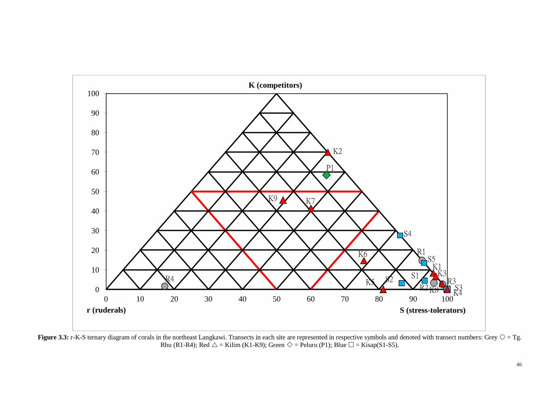
46

Figure 3.3: r-K-S ternary diagram of corals in the northeast Langkawi. Transects in each site are represented in respective symbols and denoted with transect numbers: Grey = Tg.

Rhu (R1-R4); Red = Kilim (K1-K9); Green = Peluru (P1); Blue = Kisap(S1-S5).

R1

R2 R3 R4

K1

K2

K3

S3 K5

K6

K7

K8

K9

S1 S2

K4

S4

S5

P1

0

10

20

30

40

50

60

70

80

90

100

0 10 20 30 40 50 60 70 80 90 100

K (competitors)

S (stress-tolerators) r (ruderals)

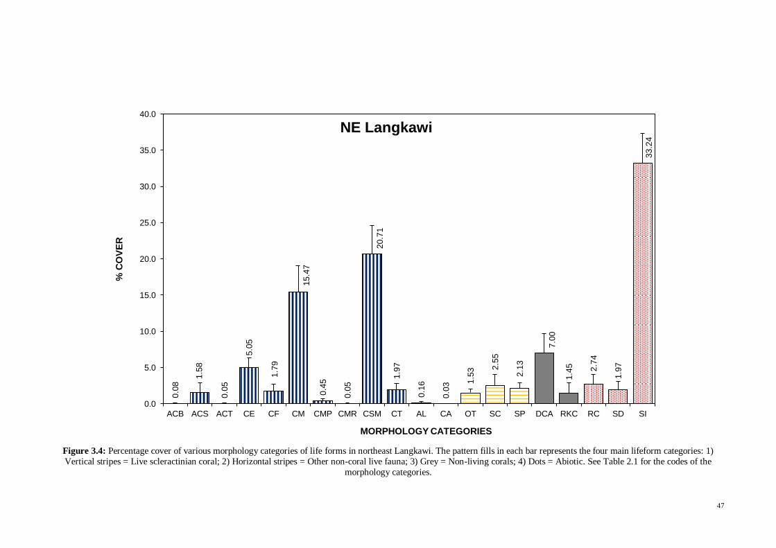
47

Figure 3.4: Percentage cover of various morphology categories of life forms in northeast Langkawi. The pattern fills in each bar represents the four main lifeform categories: 1)

Vertical stripes = Live scleractinian coral; 2) Horizontal stripes = Other non-coral live fauna; 3) Grey = Non-living corals; 4) Dots = Abiotic. See Table 2.1 for the codes of the

morphology categories.

0.0

8 1

.58

0.0

5

5.0

5

1.7

9

15.4

7

0.4

5

0.0

5

20.7

1

1.9

7

0.1

6

0.0

3 1.5

3 2.5

5

2.1

3

7.0

0

1.4

5

2.7

4

1.9

7

33.2

4

0.0

5.0

10.0

15.0

20.0

25.0

30.0

35.0

40.0

ACB ACS ACT CE CF CM CMP CMR CSM CT AL CA OT SC SP DCA RKC RC SD SI

% C

OV

ER

MORPHOLOGY CATEGORIES

NE Langkawi

48

3.4 Stomach content analysis to determine trophic guilds

The dietary composition of 54 fish species as depicted in the PCA biplot showed

the six conspicuous groupings conspicuously, namely Piscivores, Mixed Carnivores,

Omnivores, Herbivores, Prawn and Mixed Invertebrate feeders (Fig. 3.5a, 3.5b). The

Prawn and Mixed Invertebrate feeders were subsequently combined to form one trophic

guild, the Invertivores which comprised the largest number of species. Invertivores were

introduced because their ∆15

N values were significantly lower than carnivores that feed

on high-protein vertebrate animals (McCutchan et al. 2003). The first two PCA

functions, with respective eigen values of 0.289 and 0.189, explained 47.8% of the total

variance of the data (see Appendix II).

3.5 Stable isotopes of producers and consumers

The δ13

C and δ15

N dual stable isotope values of primary producers and fish

tissues are presented in Table 3.11. The mangrove plants, R. apiculata and C. tagal had

δ13

C mean values of -28.61 ± 0.17 ‰ (SE) and -29.05 ± 0.80 ‰, while their δ15

N mean

values were 3.48 ± 1.35 and 3.74 ± 1.04, respectively. Seston appeared to be more

enriched in δ13

C than mangrove detritus, with mean values of -21.64 ± 0.79. The most

enriched δ13

C values belonged to coral zooxanthellae (Zoox) with mean value of -15.39

± 0.33 ‰. The δ13

C values of reef sediment (-21.22 ± 0.31 ‰) were far from coral

zooxanthellae but close to seston, whereas the values for estuarine sediment (-26.30 ±

0.29 ‰) were closer to mangrove leaves. Primary carbon sources including sediments

ranked from depleted to most enriched δ13

C values were mangrove leaves, mangrove

sediments, estuarine seston, nearshore seston, reef sediments, mangrove creek seston,

benthic diatoms and coral zooxanthellae. Biplots of carbon sources and sediments are

illustrated in Figure 3.6a.

49

Figure 3.5: Principal component analysis (PCA) of stomach content of fishes with a) arrows denoting food consumed: Fish, Prawn, Mysid, Copepod (Cope), Malacostracas (Mala),

Crab, Molluscs (Moll), Crustaceans (Crus), Echinoderms (Echi), Plant Detritus (Detr), Polychaetes (Pcha), Diatoms (Dia), Porifera (Pori) and b) fish species grouped into their

respective feeding guilds: = Piscivores; = Carnivores; = Invertivores*; = Omnivores; = Herbivores. *The feeding guild Invertivores were made up of the combined

prawn and mixed invertebrate feeders. See Table 1 for species abbreviation.

50

Table 3.11: Mean ± SE isotope values of δ13C, δ15N and C/N ratio of the possible primary energy

sources, zooplankton and sediments. n denotes the number of samples collected for each source. *from

Okamura et al. (2010).

Sources

δ13

C (‰) δ15

N (‰) C:N

n Mean ± SE Mean ± SE Mean ± SE

Mangrove plants (Detritus)

6 -28.83 0.38 3.61 0.76 52.32 3.24

Rhizophora apiculata 3 -28.61 0.17 3.48 1.35 45.30 1.42

Ceriops tagal 3 -29.05 0.80 3.74 1.04 59.35 1.15

Phytoplankton (Seston)

15 -21.64 0.79 5.35 0.40 9.63 0.54

Coral zooxanthellae (Zoox)

23 -15.39 0.33 6.20 0.19 7.11 0.23

Benthic diatoms* (Diatoms)

3 -17.30 0.72 3.70 0.58 - -

Zooplankton 11 -21.66 0.72 7.38 0.43 5.07 0.08

Sediments (Reef) 19 -21.22 0.31 5.61 0.16 9.54 0.23

Sediments (Estuary) 17 -26.30 0.29 3.70 0.13 19.06 0.89

51

Figure 3.6: Isotopic map of δ13C and δ15N signatures of fish tissues (before trophic fractionation

correction) by (a) primary sources include coral zooxanthellae (Zoox), benthic diatoms (Diatoms), seston

or phytoplankton (Nearshore, Mangrove Estuary and Mangrove Creeks) and mangrove (Detritus), and

sediments from the coral reef (Reef Sediment) and mangrove (Mangrove Sediment); (b) Habitat zones

such as coral zone (Coral), mangrove-coral zone (Mg-C), mangrove estuary zone (Mg) and mangrove

creek zone (Up); (c) Trophic guilds. Numerals indicate mean δ13C and δ15N. All data are in mean ± SE.

c)

b)

a)

52

Kruskal-Wallis analysis revealed that trophic guilds differed significantly in

both their δ13

C (χ2 = 52.67, df = 4, p < 0.001) and δ

15N (χ

2 = 173.73, df = 4, p < 0.001)

values. Post hoc pairwise analysis suggested that trophic guilds significantly differed

(p<0.05) in terms of δ13

C between the following pairs: piscivores – invertivores,

piscivores – carnivores, piscivores – omnivores, invertivores – omnivores and

herbivores – omnivores. However, in terms of δ15

N, trophic guilds significantly differed

between all pairs except carnivores – invertivores (p<0.05) (Table 3.12; Fig. 3.6c; see

Appendix III) indicates that the trophic groupings determined by the PCA of stomach

content were satisfactory. The mean values of δ13

C, δ15

N and C/N ratio of the fish

species, assigned to respective feeding guilds, are presented in Table 3.13. Herbivorous

fishes had a large range of δ13

C mean values (-8.88 to -15.72 ‰), while their mean δ15

N

values ranged from 7.18 to 8.45 ‰. The demersal grey mullets, Moolgarda perusii,

Moolgarda seheli and Valamugil buchanani, were found in both reef and mangrove

suggesting that these species move between these habitats.

Table 3.12: Results of Kruskal-Wallis non-parametric test and post hoc Wilcoxon Mann-Whitney test.

Significant difference are at *p<0.001. Pairs of insignificant difference are denoted by the same letters.

Isotopic

composition

Kruskal-Wallis

Test*

Post hoc Wilcoxon Mann-Whitney Test df χ

2

δ13

C 4 51.67

Herbivores

a, Omnivores

a,b,c, Invertivores

b,c, Carnivores

c,

Piscivoresc,

δ15

N 4 173.72

Herbivores, Omnivores, Invertivores

a, Carnivores

a,

Piscivores

δ13

C 3 33.76

Coral, Mg-Ca, Mg

a, Up

δ15

N 3 53.66

Corala, Mg-C

a, Mg

b, Up

b

Another species of mullet also found in both habitats, Ellechelon vaigiensis was

classified as omnivorous based on PCA. This is corroborated by its δ15

N value of 9.52

‰, which reflects a higher trophic position than other herbivorous members of the

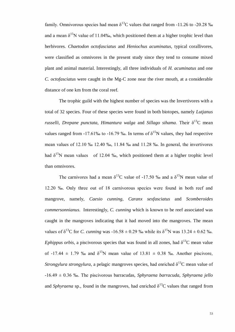
53

family. Omnivorous species had mean δ13

C values that ranged from -11.26 to -20.28 ‰

and a mean δ15

N value of 11.04‰, which positioned them at a higher trophic level than

herbivores. Chaetodon octofasciatus and Heniochus acuminatus, typical corallivores,

were classified as omnivores in the present study since they tend to consume mixed

plant and animal material. Interestingly, all three individuals of H. acuminatus and one

C. octofasciatus were caught in the Mg-C zone near the river mouth, at a considerable

distance of one km from the coral reef.

The trophic guild with the highest number of species was the Invertivores with a

total of 32 species. Four of these species were found in both biotopes, namely Lutjanus

russelli, Drepane punctata, Himantura walga and Sillago sihama. Their δ13

C mean

values ranged from -17.61‰ to -16.79 ‰. In terms of δ15

N values, they had respective

mean values of 12.10 ‰ 12.40 ‰, 11.84 ‰ and 11.28 ‰. In general, the invertivores

had δ15

N mean values of 12.04 ‰, which positioned them at a higher trophic level

than omnivores.

The carnivores had a mean δ13

C value of -17.50 ‰ and a δ15

N mean value of

12.20 ‰. Only three out of 18 carnivorous species were found in both reef and

mangrove, namely, Caesio cunning, Caranx sexfasciatus and Scomberoides

commersonnianus. Interestingly, C. cunning which is known to be reef associated was

caught in the mangroves indicating that it had moved into the mangroves. The mean

values of δ13

C for C. cunning was -16.58 ± 0.29 ‰ while its δ15

N was 13.24 ± 0.62 ‰.

Ephippus orbis, a piscivorous species that was found in all zones, had δ13

C mean value

of -17.44 ± 1.79 ‰ and δ15

N mean value of 13.81 ± 0.38 ‰. Another piscivore,

Strongylura strongylura, a pelagic mangroves species, had enriched δ13

C mean value of

-16.49 ± 0.36 ‰. The piscivorous barracudas, Sphyraena barracuda, Sphyraena jello

and Sphyraena sp., found in the mangroves, had enriched δ13

C values that ranged from

54

-15.56 to -17.88 ‰. On average, fish classified as piscivores had a relatively enriched

δ13

C value of -16.72 ± 1.49 ‰ and δ15

N value of 13.30 ± 0.78 ‰.

Biplots of the δ13

C and δ15

N values of the fish trophic guilds are given in Fig.

3.6c. The most enriched δ13

C value belonged to herbivores (-14.33 ± 0.43 ‰), whereas

the most depleted were mixed carnivores (-17.50 ± 0.21 ‰). The range of these δ13

C

values overlapped the values of benthic diatoms and coral zooxanthellae, but the values

were quite far from those of seston and mangrove (Fig. 3.6a). In terms of δ15

N values,

the piscivores (13.30 ± 0.16 ‰) were the most enriched with respect to the herbivores

(8.04 ± 0.15 ‰). The trophic guilds ranked in terms of δ15

N enrichment are as follows:

herbivores, omnivores, invertivores, carnivores and piscivores.

55

Table 3.13: Mean and ±SE tissues isotopes of δ13C, δ15N (both expressed in ‰) and C/N ratio of fish species (grouped into respective feeding guilds) with number of samples

collected (n) in each zone.

Sp. Abbrv./

Refs.

n δ13C δ15N C:N

Species Coral

Reefs

Mangrove-

Coral

Mangrove

Estuary

Mangrove

Creeks Total Mean ± SE Mean ± SE Mean ± SE

Herbivore 65 -14.33 0.43 8.04 0.15 3.83 0.01

Anodontostoma chacunda Anch 0 3 7 4 14 -15.27 0.61 8.39 0.21 3.86 0.03

Chelon subviridis Chsu 1 0 13 2 16 -15.72 0.84 8.45 0.17 3.74 0.02

Moolgarda perusii (a) 4 0 5 0 9 -11.70 0.46 7.44 0.53 3.93 0.04

Moolgarda seheli Mose 2 5 10 3 20 -13.90 0.84 7.98 0.11 3.82 0.01

Paramugil parmatus (b) 1 0 0 0 1 -8.88 0.00 7.47 3.82

Valamugil buchanani Vabu 2 1 0 2 5 -14.80 2.38 7.18 1.37 3.83 0.04

Omnivore 47 -15.74 0.50 11.04 0.24 3.81 0.02

Anodontostoma thailandiae Anth 0 0 1 0 1 -20.28 0.00 9.18 3.69

Chaetodon octofasciatus (d) 2 1 0 0 3 -13.03 0.41 11.90 0.11 3.79 0.03

Dendrophyssa russelli Deru 0 0 2 0 2 -19.71 0.05 11.28 0.07 3.75 0.06

Ellochelon vaigiensis (c) 3 2 0 3 8 -11.26 0.14 9.52 0.41 3.74 0.01

Gerres filamentosus Gefi 0 0 6 3 9 -17.46 0.81 10.95 0.29 3.81 0.03

Gerres oyena Geoy 4 0 2 0 6 -13.42 0.40 11.80 0.18 3.77 0.02

Heniochus acuminatus (d) 0 3 0 0 3 -17.50 0.08 13.80 0.20 4.18 0.12

Leiognathus splendens Lesp 0 0 4 0 4 -16.95 2.37 8.12 0.40 3.91 0.02

Monachanthus chinensis Moch 0 4 0 0 4 -16.00 0.32 12.64 0.44 3.74 0.01

Siganus javus Sija 2 2 0 1 5 -19.35 1.28 11.71 0.41 3.75 0.02

Triacanthus biaculeatus Trbi 0 0 2 0 2 -16.05 0.01 11.54 0.60 3.82 0.00

56

Sp.

Abbrv./

Refs.

n δ13C δ15N C:N

Species Coral

Reefs

Mangrove-

Coral

Mangrove

Estuary

Mangrove

Creeks Total Mean ± SE Mean ± SE Mean ± SE

Invertivore 84 -16.67 0.28 12.04 0.15 3.78 0.01

Ambassis nalua (e) 0 0 1 1 2 -19.93 0.67 12.37 0.01 3.77 0.02

Secutor ruconius (f) 0 1 0 0 1 -16.62 13.00 3.73

Stolephorus indicus (g) 0 0 1 0 1 -16.88 13.19 3.76

Abudefduf vaigiensis Abva 1 0 0 0 1 -18.27 11.69 3.75

Acentrogobius caninus (h) 0 0 1 0 1 -16.59 11.56 3.71

Cynoglossus cynoglossus (i) 0 0 1 0 1 -17.47 10.58 3.72

Drepane punctate Drpu 2 5 4 0 11 -17.61 0.79 12.40 0.27 3.80 0.03

Epinephelus coioides Epco 2 2 0 3 7 -17.35 1.24 12.93 0.61 3.75 0.01

Epinephelus erythrurus Eper 1 0 0 0 1 -13.17 12.15 3.78

Epinephelus sexfasciatus Epse 2 0 0 0 2 -15.98 0.14 13.30 0.34 3.80 0.02

Eubleekeria jonesi Eujo 0 0 2 0 2 -15.55 0.21 10.43 0.08 3.84 0.03

Eubleekeria splendens Eusp 0 0 1 0 1 -14.87 11.81 3.78

Gerres erythrourus Geer 0 0 4 0 4 -14.34 0.57 10.17 0.34 3.88 0.05

Himantura walga Hiwa 1 0 1 0 2 -16.79 2.12 11.84 0.33 3.43 0.06

Ilisha melastoma (g) 0 0 2 0 2 -19.30 0.73 11.94 0.28 3.78 0.01

Johnius belangerii (j) 0 1 0 0 1 -16.37 13.59 3.75

Lagocephalus lunaris Lalu 0 0 1 0 1 -14.03 11.32 3.80

Leiognathus brevirostris Lebr 0 3 5 0 8 -15.46 0.23 11.75 0.34 3.80 0.02

Leiognathus daura Leda 3 0 0 0 3 -16.54 0.13 13.30 0.24 3.78 0.02

Leiognathus equulus Leeq 0 2 0 0 2 -14.97 0.21 10.52 0.17 3.84 0.03

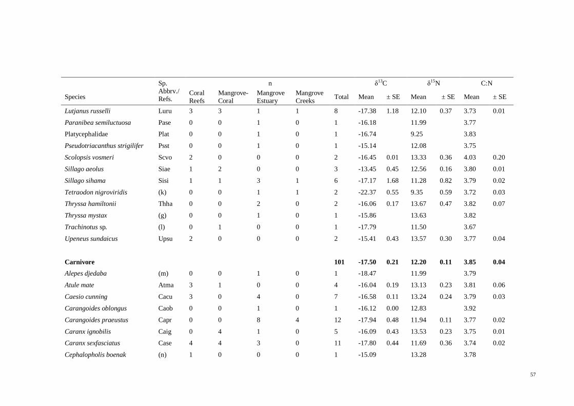
57

Sp.

Abbrv./

Refs.

n δ13C δ15N C:N

Species Coral

Reefs

Mangrove-

Coral

Mangrove

Estuary

Mangrove

Creeks Total Mean ± SE Mean ± SE Mean ± SE

Lutjanus russelli Luru 3 3 1 1 8 -17.38 1.18 12.10 0.37 3.73 0.01

Paranibea semiluctuosa Pase 0 0 1 0 1 -16.18 11.99 3.77

Platycephalidae Plat 0 0 1 0 1 -16.74 9.25 3.83

Pseudotriacanthus strigilifer Psst 0 0 1 0 1 -15.14 12.08 3.75

Scolopsis vosmeri Scvo 2 0 0 0 2 -16.45 0.01 13.33 0.36 4.03 0.20

Sillago aeolus Siae 1 2 0 0 3 -13.45 0.45 12.56 0.16 3.80 0.01

Sillago sihama Sisi 1 1 3 1 6 -17.17 1.68 11.28 0.82 3.79 0.02

Tetraodon nigroviridis (k) 0 0 1 1 2 -22.37 0.55 9.35 0.59 3.72 0.03

Thryssa hamiltonii Thha 0 0 2 0 2 -16.06 0.17 13.67 0.47 3.82 0.07

Thryssa mystax (g) 0 0 1 0 1 -15.86 13.63 3.82

Trachinotus sp. (l) 0 1 0 0 1 -17.79 11.50 3.67

Upeneus sundaicus Upsu 2 0 0 0 2 -15.41 0.43 13.57 0.30 3.77 0.04

Carnivore 101 -17.50 0.21 12.20 0.11 3.85 0.04

Alepes djedaba (m) 0 0 1 0 1 -18.47 11.99 3.79

Atule mate Atma 3 1 0 0 4 -16.04 0.19 13.13 0.23 3.81 0.06

Caesio cunning Cacu 3 0 4 0 7 -16.58 0.11 13.24 0.24 3.79 0.03

Carangoides oblongus Caob 0 0 1 0 1 -16.12 0.00 12.83 3.92

Carangoides praeustus Capr 0 0 8 4 12 -17.94 0.48 11.94 0.11 3.77 0.02

Caranx ignobilis Caig 0 4 1 0 5 -16.09 0.43 13.53 0.23 3.75 0.01

Caranx sexfasciatus Case 4 4 3 0 11 -17.80 0.44 11.69 0.36 3.74 0.02

Cephalopholis boenak (n) 1 0 0 0 1 -15.09 13.28 3.78

58

Sp.

Abbrv./

Refs.

n δ13C δ15N C:N

Species Coral

Reefs

Mangrove-

Coral

Mangrove

Estuary

Mangrove

Creeks Total Mean ± SE Mean ± SE Mean ± SE

Epinephelus bleekeri Epbl 4 3 0 0 7 -15.67 0.45 13.37 0.18 3.82 0.02

Epinephelus malabaricus (l) 0 2 0 0 2 -20.88 1.62 10.86 0.80 3.75 0.03

Hexanematichthys sagor (o) 0 0 1 1 2 -19.29 0.83 9.95 0.51 3.75 0.04

Lutjanus johnii Lujo 0 3 0 0 3 -16.49 0.86 12.19 0.39 3.74 0.04

Lutjanus lutjanus Lulu 3 0 0 0 3 -16.87 0.03 13.00 0.22 3.81 0.02

Lutjanus vitta Luvi 3 0 0 0 3 -16.29 0.20 13.20 0.12 3.82 0.02

Nemipterus hexodon (p) 0 3 0 0 3 -12.90 0.21 12.41 0.19 3.96 0.04

Plectorhinchus gibbosus Plgi 0 8 0 0 8 -19.31 0.76 12.22 0.33 4.59 0.41

Pomadasys kaakan Poka 0 2 10 1 13 -18.80 0.67 10.69 0.24 3.82 0.07

Scomberoides

commersonnianus Scco 1 0 11 3 15 -17.95 0.60 12.35 0.22 3.78 0.02

Piscivore 25 -16.72 0.30 13.30 0.16 3.78 0.01

Alepes kleinii Alkl 0 1 0 0 1 -16.41 13.66 3.79

Elops machnata Elma 0 0 1 0 1 -13.63 11.76 3.75

Ephippus orbis Epor 2 3 1 2 8 -17.44 0.63 13.81 0.13 3.83 0.03

Scomberoides lysan Scly 0 4 1 0 5 -16.32 0.08 13.13 0.12 3.80 0.03

Scomberoides tol Scto 1 0 0 0 1 -16.29 13.10 3.84

Sphyraena barracuda (e) 0 0 1 0 1 -17.88 12.54 3.68

Sphyraena jello Spje 0 1 2 0 3 -15.92 0.97 13.27 0.99 3.74 0.01

Sphyraena sp. (e) 0 0 1 0 1 -15.56 12.09 3.73

Strongylura strongylura (q) 0 0 2 0 2 -16.49 0.25 13.68 0.16 3.74 0.04

59

Sp.

Abbrv./

Refs.

n δ13C δ15N C:N

Species Coral

Reefs

Mangrove-

Coral

Mangrove

Estuary

Mangrove

Creeks Total Mean ± SE Mean ± SE Mean ± SE

Tylosurus crocodilus

crocodilus Tycc 0 0 1 1 2 -18.13 0.96 13.05 0.14 3.73 0.02

*Sp. abbrv. is the abbreviation of fish species for PCA in Fig. 3.5 b), while Ref. is the references used to assign fish species into their respective feeding guild as stomach

content data were not available and empty.

References: (a) Kanou & Sano, 2004; (b) closest species to C. subviridis; (c) Nanjo, Kohno, & Sano, 2008; (d) Cole, Pratchett, & Jones, 2008; (e) Abrantes & Sheaves, 2009;

(f) Liu, 1997; (g) Then, 2009; (h) Maugé, 1986; (i) Munroe, 2001; (j) Sasaki, 2001; (k) Shinnaka et al., 2007; (l) Smith-Vaniz, 1999; (m) Raje, 1993; (n) Beukers-Stewart &

Jones, 2004; (o) Hajisamae, Chou, & Ibrahim, 2004; (p) Salini, Blaber, & Brewer, 1994; (q) Baker & Sheaves, 2005.

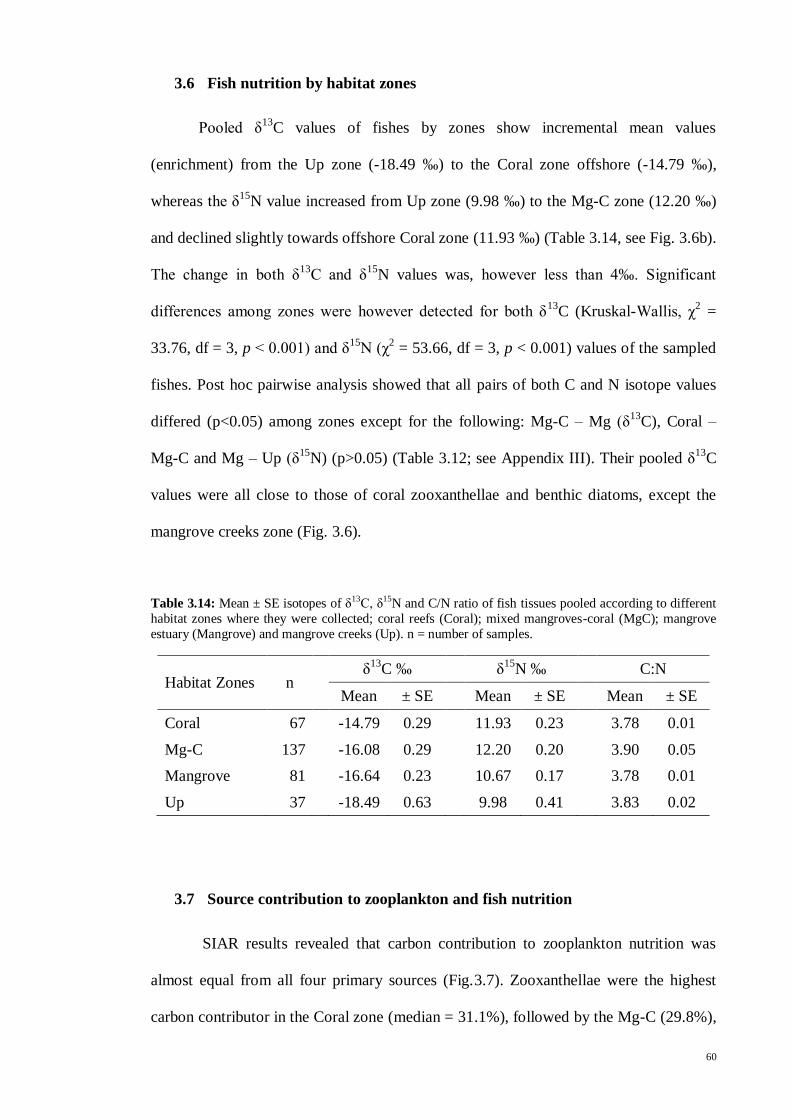
60

3.6 Fish nutrition by habitat zones

Pooled δ13

C values of fishes by zones show incremental mean values

(enrichment) from the Up zone (-18.49 ‰) to the Coral zone offshore (-14.79 ‰),

whereas the δ15

N value increased from Up zone (9.98 ‰) to the Mg-C zone (12.20 ‰)

and declined slightly towards offshore Coral zone (11.93 ‰) (Table 3.14, see Fig. 3.6b).

The change in both δ13

C and δ15

N values was, however less than 4‰. Significant

differences among zones were however detected for both δ13

C (Kruskal-Wallis, χ2 =

33.76, df = 3, p < 0.001) and δ15

N (χ2 = 53.66, df = 3, p < 0.001) values of the sampled

fishes. Post hoc pairwise analysis showed that all pairs of both C and N isotope values

differed (p<0.05) among zones except for the following: Mg-C – Mg (δ13

C), Coral –

Mg-C and Mg – Up (δ15

N) (p>0.05) (Table 3.12; see Appendix III). Their pooled δ13

C

values were all close to those of coral zooxanthellae and benthic diatoms, except the

mangrove creeks zone (Fig. 3.6).

Table 3.14: Mean ± SE isotopes of δ13C, δ15N and C/N ratio of fish tissues pooled according to different

habitat zones where they were collected; coral reefs (Coral); mixed mangroves-coral (MgC); mangrove

estuary (Mangrove) and mangrove creeks (Up). n = number of samples.

Habitat Zones n δ

13C ‰ δ

15N ‰ C:N

Mean ± SE Mean ± SE Mean ± SE

Coral 67 -14.79 0.29 11.93 0.23 3.78 0.01

Mg-C 137 -16.08 0.29 12.20 0.20 3.90 0.05

Mangrove 81 -16.64 0.23 10.67 0.17 3.78 0.01

Up 37 -18.49 0.63 9.98 0.41 3.83 0.02

3.7 Source contribution to zooplankton and fish nutrition

SIAR results revealed that carbon contribution to zooplankton nutrition was

almost equal from all four primary sources (Fig.3.7). Zooxanthellae were the highest

carbon contributor in the Coral zone (median = 31.1%), followed by the Mg-C (29.8%),

61

Mg (26.3%) and Up (13.8%) zones. The highest carbon contribution to zooplankton

nutrition in the Up zone came from mangrove detritus (38.8%). Mangrove detritus also

contributed to zooplankton nutrition in the Mg zone (27.9%), Mg-C zone (22.5%) and

Coral zone (26.3%). Zooplankton dependence on seston was about equal for all zones;

25.2% in Coral, 25.3% in Mg-C, 25.0% in both Mg and Up zones, respectively. Benthic

diatoms were the lowest carbon contributor to zooplankton nutrition; 17.4% in the Coral

zone, 23.2% in the Mg-C, 21.6% in the Mg zone and 18.3% in the Up zone (see

Appendix IV).

Figure 3.7: Proportional contribution of coral zooxanthellae (Zooxanthellae); phytoplankton (Seston);

benthic diatoms (Diatom) and mangrove (Detritus) to zooplankton nutrition in different habitat zones of a coupled coral-mangrove ecosystem in Langkawi, Malaysia. Coral reefs (Coral); mangroves-corals (Mg-

C); mangrove (Mg) and mangrove creeks (Up) as determined by Stable Isotope Analysis in R. Bars shows

Bayesian confidence intervals of 50, 75 and 95%.

In contrast to zooplankton, the SIAR results indicated a relatively high source

contribution of carbon from zooxanthellae to fish followed by seston in all four zones

62

(Fig. 3.8). Zooxanthellae contribution in the Coral zone was the highest at

approximately 90.0% (median) and decreased in the landward direction through the

mixed Mg-C zone (72.7%), the Mg zone (63.7%), to the Up zone (38.4%). Seston was

the second major contributor to fish nutrition, with an estimated 6.0% in the Coral zone

which increased to 22.6%, 32.0% and 38.4% in the Mg-C, Mg and Up zones

respectively. In the Up zone, fish dependence on carbon was multi-sourced with benthic

diatoms contributing 8.1% and mangrove 12.7%. Carbon signature of mangrove and

benthic diatoms was very weak for fishes in the Coral, Mg-C and Mg zones, where both

carbon sources contributed less than 2.9% (see Appendix V).

Figure 3.8: Proportional contribution of coral zooxanthellae (Zooxanthellae); phytoplankton (Seston

from mangrove creeks, mangrove estuary and nearshore waters); benthic diatoms (Diatom) and mangrove

(Detritus) to fish nutrition in different habitat zones of a coupled coral-mangrove ecosystem in Langkawi,

Malaysia. Coral reefs (Coral); mangroves-corals (Mg-C); mangroves (Mg) and mangrove creeks (Up) as

determined by Stable Isotope Analysis in R. Bars shows Bayesian confidence intervals of 50, 75 and 95%.

63

4.0 DISCUSSION

4.1 Source contribution to fish community

The present study suggests that fishes in Langkawi’s coral-mangrove system are

supported by carbon sources primarily from coral zooxanthellae and secondarily from

phytoplankton. Their combined contribution amounts to 96% in both the Coral and Mg

zones (Fig. 3.8), whereas mangrove and benthic diatom contribution are only marginal.

Zooxanthellae contribution to fish nutrition is important in three of the zones, Coral,

Mg-C and Mg, which was estimated to be more than 60% but recorded a drop in the Up

zone. While zooxanthellae contribution shows a decreasing trend, phytoplankton

contribution increases towards the Up zone. Mangrove detritus and diatom contribution

becomes more apparent in the Up zone with reduced zooxanthellae contribution.

Similarly, zooxanthellae contribution to zooplankton nutrition also follows a decreasing

trend towards the Up zone (Fig. 3.7) suggesting the outer limits of its contribution from

the coral reefs.

The mean δ13

C signature of fishes in the Up zone (-18.49 ‰) was more depleted

than coral zooxanthellae (-15.39 ‰) and closer to seston (-21.64 ‰) as compared to the

fishes from other zones. The mean δ13

C signature of bottom sediment at the Mg zone (-

26.30 ‰) was distant from that of coral zooxanthellae, further indicating that the energy

transport fell short at the estuary. Evidently, distance limits the influence of coral

zooxanthellae which decreases towards the Up zone, i.e. farther from the reef.

Nevertheless, coral zooxanthellae are still an important source of nutrition for fish

communities in the Mg and Up zones due to their significant contribution of 63.7% and

38.4%, respectively (Fig. 3.8). This suggests an energy transfer pathway from

zooxanthellae to consumers.

However, direct energy transfer from coral zooxanthellae to consumers is

uncertain except for only one specialized group of species that directly feed on the coral

64

polyps (Cole et al., 2008; Glynn, Stewart, & McCosker, 1972). Another possible

pathway of energy transfer is via the extrusion of coral mucus (Yonge, 1972). The δ13

C

value of coral mucus was reported to be similar and corresponds to the δ13

C value of

coral zooxanthellae (Naumann et al., 2010). Our zooxanthellae δ13

C value of -15.4 ±

0.33 ‰ (see Table 12) is within the range of reported coral mucus signatures of between

-15.2 ± 0.20 ‰ to -16.2 ± 0.40 ‰ (Naumann et al., 2010; Wyatt et al., 2012).

The above finding suggests that the trophic pathway from source to consumers

is likely mediated by coral mucus. This pathway is possible because zooxanthellae are

responsible for supplying trophic energy through translocation of the photosynthetically

fixed carbon to their coral hosts (Muscatine, McCloskey, & Marian, 1981; Tremblay,

Grover, Maguer, Legendre, & Ferrier-Pagès, 2012). Up to half of this assimilated

carbon is eventually used to synthesize coral mucus, which is then released into the

water column (Crossland, Barnes, & Borowitzka, 1980; Davies, 1984). Mucus can be

slowly dislodged from the coral surface by water movements (Coles & Strathmann,

1973) and becomes suspended mucus flocs. Subsequently, the mucus flocs are then

enriched by particulate organic matter (POM) and microbial communities that adhered

to them (Wild et al., 2004; Naumann et al., 2009). Hence, mucus flocs with lower C/N

ratio are a potential food source for zooplankton (Richman et al., 1975), invertebrates

and fishes (Johannes, 1967; Benson & Muscatine, 1974; Wyatt 2011).

Phytoplankton appears to be the next preferred food by both zooplankton and

fish, especially those in the Mg and Up zones. In a recent study, Chew et al. (2012)

showed that phytoplankton supplies energy to zooplankton and small fishes in turbid

water mangroves. The findings of Chew et al. (2012) suggest that zooplankton can

assimilate carbon from phytoplankton (Fig. 3.7). The phytoplankton contribution to the

fish community, however, is likely through multiple trophic levels of prey and predator

known as trophic relay (Kneib, 2002). Stomach content analysis of large fish revealed

65

that small fishes are among the highly consumed food items (Fig. 3.7), suggesting that

large piscivores and carnivores consumed these small phytoplankton-dependent fishes.

This is further evident from the δ13

C values of the predators, which were slightly closer

to phytoplankton than the rest. Aside from that, their δ13

C values reflect that of fishes in

the Mg and Up zones (Fig. 3.6) where zooxanthellae contribution decreased. This

trophic pathway is feasible because predators are found deep in the mangroves (Table

3.13).

Despite this, mangrove contribution to overall nutrition of fish appeared to be

marginal. For instance, zooplankton in the Up zone relies on detritus to almost 40%, but

this is not highly reflected in fishes, suggesting that the mangrove detritus contribution

is limited. This concurs with some insights from stable isotopic studies of late that

dispute the mangrove detritus contribution to higher consumers (fishes). Bouillon et al.

(2008) discussed and reviewed that contribution of mangrove detritus is uncertain and

most likely to be very limited. Studies have also shown that when nutritious sources are

made available, some species tend to rely on these sources rather than mangrove detritus

(Nagelkerken et al., 2008). Despite being rich in carbon, the nitrogen content in

mangrove leaf litter is often poor (high C/N ratio), which reduces its nutritious value.

The high tannin and lignocellulose content of mangrove detritus causes indigestion and

makes it less favourable food for consumers with the exception of some crab species

(Wolcott & O’Connor, 1992).

Overall, stomach content analysis revealed that benthic invertebrates (prawns,

polychaetes, crabs) and small fishes are the most highly consumed food items of

predatory fishes (Fig. 3.5). Stomach content of the demersal and benthic species

revealed a high volume of prawns and other crustaceans consumed, whereas the pelagic

fish C. cunning (both in mangrove and coral reef) revealed the presence of prawns. This

indicates that carbon was derived from benthic invertebrates, which could consume

66

settled coral mucus, benthic diatoms and phytoplankton. The intermediate δ13

C

signatures of predatory fishes (invertivores, carnivores and piscivores) lying between

that of phytoplankton and coral zooxanthellae sources (Fig. 3.6) showed that the

consumed benthic invertebrates were dependent on a mix of the aforementioned

sources. This also explains the significant contributions of these sources to the fish

community in the mangrove (Fig. 3.7). These observations illustrate that the energy

transfer from sources to fish consumers is via trophic relay.

4.2 Physical attributes of biotopes

In the Coral zone, the turbidity is considered moderate to high, with a mean of

25.87 ± 7.70 NTU (Table 3.2) and ranging from as low as one NTU to as high as 140

NTU. This is comparable to reports from natural turbid water reefs in Palumo Shoals,

Australia, where a turbidity range of 0 – 15 NTU is considered low while high turbidity

ranges from 50 – 200 NTU (Anthony & Larcombe, 2000; Larcombe, Costen, & Woolfe,

2001). High turbidity attenuates the light intensity, which is necessary for

endosymbiotic zooxanthellae for photosynthesis. Consequently, the physiological

processes and growth of the host corals are affected (Rogers, 1990). However, various

adaptive mechanisms by corals have enabled them to survive in naturally turbid and

high sedimentation environments (Anthony & Larcombe, 2000). Under turbid

conditions, corals are known to produce substantial amounts of mucus to waft sediments

from their surface (Hubbard & Pocock, 1972; Yonge, 1972; Schuhmacher, 1977). A

similar condition is observed in northeast Langkawi as the coral reefs here are exposed

to moderate turbidity, yet are low in mortality (Table 3.10). Nonetheless, the turbidity

measurements between coral reef and mangrove estuary are highly similar resulting in

an equal predation risk in both habitats which offer fishes larger refuge area.

67

Turbidity has been hypothesized to reduce the predation pressure because it

affects the reaction rate of predatory fishes (Benfield & Minello, 1996; Nagelkerken,

2009b). The suspended particles in turbid water scatter light and reduce the reaction rate

of predators, consequently reducing predatory success (Benfield & Minello, 1996). It is

one of the factors that attract fishes to brackish water habitats such as mangroves (Cyrus

& Blaber, 1987). The similar turbidity recorded in the coral reefs of northeast Langkawi

suggests that fishes would be equally attracted to coral reefs.

Although some of the differences in physical attributes, the zones are significant

according to statistical test, their difference margins are small, less than 2 units (Table

3.2). All measurements of the attributes were carried out as point measurements which

may not reflect the long term average, but are sufficient to measure the general physical

attributes of the seawater because they did not fluctuate drastically, with exception of

turbidity. Furthermore, measurements were carried out at many stations, resulting in

large numbers of replicates, thus giving a sufficient representation for each attribute.

The numbers of replicates for DO and ORP were different from the rest of the attributes

because the respective probes malfunctioned during the sampling trip and did not record

any readings (Table 3.1).

The measured physical attributes for coral reefs showed that the seawater

condition was relatively stressful for corals. All readings of attributes for the mangroves

were, however, within the tolerable range because of their robustness and high degree of

ecological stability (Alongi, 2008; Giesen, Wulffraat, Zieren, & Scholten, 2006).

Mangroves are well adapted to harsh environment as they are subjected to daily tidal

changes in temperature, salinity and different degrees of anoxia (Alongi, 2008).

Conversely, coral reefs are steno-tolerant and susceptible to even small environmental

changes (Kleypas et al., 1999). The measurements of the attributes in coral reef area

were found to be slightly lower than the reported measurements from Tuba Island, south

68

of Langkawi (Jalal et al., 2009), except for temperature, which was slightly higher in the

present study. The temperature readings recorded in the present study were within the

range as reported by Chong et al. (2005) at the same study sites. The temperature in all

zones reflect the typical tropical seawater temperature that ranges from 18 °C to 30 °C,

except in the Coral zone, which was measured at the mean of 30.57 °C. This mean

temperature, however, is still within the upper thermal limit of scleractinian corals of

between 31°C to 32°C, hence the coral reef of Langkawi can be categorised as a

marginal reef (Kleypas et al., 1999).

The reef’s mean salinity, which was measured at 31.96 ± 0.16 ppt, is considered

low and corroborates its categorisation as a marginal reef. Coral reefs with average

seawater salinity outside the range of 34 – 36 ppt will be affected in their coral

physiology (Moberg, Nyström, Kautsky, Tedengren, & Jarayabhand, 1997; Sheppard,

Davy, & Pilling, 2009). The relatively low salinity of the Coral zone in Langkawi is due

to freshwater inputs from nearby small rivers. However, tidal exchanges create a salinity

gradient from the Coral zone to the zone nearest to freshwater source, the Up zone.

Nevertheless, some corals have been reported to be able to adapt and respond

physiologically to salinity changes (Moberg et al., 1997), especially in an area where

there are freshwater discharges from rivers, similar to the conditions found in the

present study site.

The measured pH ranged from 7 – 8, within the basic water condition of

nearshore seawater. The readings corroborate with the reported pH from Tuba Island,

(Jalal et al., 2009) which generally indicates no signs of detrimental water quality with

regards to acidity. However, since the present site is within a limestone karst, any fall in

pH could have been buffered by this. Although no measurement of water chemical

attributes was done, Rau et al. (2007) reported that an increase of pH (acidity reduced)

69

is possible from accelerated weathering of limestone through seawater reactions with

bicarbonate ions.

The measurements of the physical attributes of the current study sites provide

useful information of the present status of both coral and mangrove habitats. This

information allows an evaluation of whether development affects the marine organisms

and consequently, the connectivity between both habitats. Kilim area has been

developed over the past decade, especially during the last few years, since the

declaration of its Geoforest Park by UNESCO in 2007. These developments, together

with the expansion of the tourism industry, have contributed to the habitat degradation,

especially of the mangrove forests (Shahbudin et al., 2012). Jalal et al. (2009) reported

that due to the rapid development of the tourism industry, Langkawi has been

increasingly polluted during the last decade. Thus, it is imperative to conserve and

protect both habitats from further destruction.

4.3 Fish species diversity and similarity

It is evident that the coral reef biotope comprising of only Coral zone is

connected to the mangrove biotope, which consists of the Mg and Up zones (Fig. 2.3)

via overlapping or common fish fauna (Fig. 4.1). For the present study, the zones at

both ends of the study area, the Coral zone (TC, KC and SC) and the Up zone (TMU,

KMU and SMU) show similar species composition indicating reef fish species are

likely to move deeper into the mangrove zone and vice versa (Fig. 3.1). Although the

fish species composition in the Mg zone (TM, KM, PM and SM) is slightly different

from that of the Coral zone, the linkage distance of disagreement is only marginally

more than half or 61% (Fig. 3.2), indicating that there is still some degree of similarity

in fish species composition between the zones. The overall total of 31 common species

listed (Table 3.6) constitutes approximately 21.1% of the total fish species (including

70

species from previous studies) in northeast Langkawi. The number of common fishes is

considerably high, as other studies have reported as low as only 6 and up to 43 common

species between reef and non-reef habitats (Laroche et al., 1997; Nagelkerken, 2007;

Thollot & Thollot, 1992). This indicates a fairly high exchange of fish species between

habitats, which suggests a relatively strong connectivity (Chittaro et al., 2005).

Figure 4.1: Illustration of the 31 common species (blue region) found in both coral (orange region) and

mangrove (green region) biotopes. Full species names as given in the indicated table.

The relatively high turbidity levels at Langkawi’s north eastern reefs and

mangroves result in low visibility, rendering the visual census of fishes by diving

difficult. Thus, traditional fishing methods such as gill nets and “bubu” had to be used

in both coral reefs and mangroves to reduce spatial bias. The same fishing methods had

similarly been applied to both biotopes to enable comparisons (Nagelkerken, 2007).

Nevertheless, catches from these passive fishing gears are expected to be an

underestimation (Olin, Malinen, & Ruuhijärvi, 2009). Although there were replicates,

the incorporation of other species from previous studies into the present species list has

resulted in a clearer picture of the fish composition in the study area. Chong et al.

(2005) reported a total of 91 species from 42 families, 6 species less but 4 families more

71

than in the present study of 97 species from 38 families. The incorporation of the

previous data, however, included an additional 50 species from 14 families to the

current study resulting in a total of 147 species from 52 families. This indicates that

only 41 species from previous studies were caught again, whereas 56 species had not

been previously found. Such a large difference is attributed to the use of different types

of fishing gear as well as spatial differences in sampling. The fishing gear deployed in

previous studies included gill nets, cast net and beam trawl, while only gill nets and

“bubu” were deployed in the present study. Furthermore, Chong et al. (2005) carried out

their sampling within a shorter period and did not sample in the coral reef. Although gill

net is highly selective, it is deemed a more suitable gear and effective in catching

actively mobile fishes (Olin et al. 2009), which are the key subjects connecting the

biotopes. Ideally, a combination of multiple active and passive types of fishing gear

should be used to ensure adequate catch of fishes (Olin et al., 2009; Rotherham,

Johnson, Kesby, & Gray, 2012). Nevertheless, applying multiple fishing gear requires a

higher amount of labour. Thus, the combination of previous and present results is the

best way to obtain a comprehensive species list for both biotopes in northeast

Langkawi.

The nursery function of mangroves in northeast Langkawi is explored by

differentiating between juvenile and adult sizes for each common species listed in this

study (Table 3.7). Several studies compared only the densities of juveniles in different

biotopes in order to determine the significance of nursery habitat, but such

generalizations should be avoided (Chittaro et al., 2005). A habitat could still potentially

serve as a nursery despite having lower densities of juvenile species and vice versa.

Some studies found that densities of juveniles were either equivalent or lower in the

nursery than in the adult habitat (Chittaro et al., 2005; Dorenbosch et al., 2005;

Nagelkerken & van der Velde, 2002). Similarly, although not in the terms of density

72

measures, the present study has shown that the number of common species in the

juvenile stage was low. Only 10 species in the mangrove biotope and 9 in the coral reef

are in the juvenile stage, which constituted half the number of species in the adult stage

for both of the biotopes (Fig. 4.2). This is an interesting finding because a higher

number of juvenile species was expected due to the higher species richness in the

mangrove biotope (Mg and Up zones) which was 98 species as compared to the coral

reef biotope of 59 species (Fig. 4.1). Even this is an interesting finding because it

contrasts with the findings reported elsewhere, where higher fish species richness was

reported in the reefs than in the mangroves (Dorenbosch et al., 2005; Honda, Nakamura,

Nakaoka, Uy, & Fortes, 2013; Jaxion-Harm et al., 2012; Nagelkerken & van der Velde,

2002).

Figure 4.2: Illustration of juvenile and adult common species between coral reef and mangrove biotopes.

The lighter shades of colour on the above represent species in juvenile stage while the lower darker

shades of colour represent species in adult stage. The blue region represents the species that had both the

juvenile and adult stages in both habitats.

The often reported nursery value of mangroves to fish may be contentious given

that the measuring methods are surrounded with controversy. Standard measurements

could not be agreed on among ecologists, causing difficulty in determining the value of

73

mangroves as nursery habitat for fish from other biotopes (Nagelkerken et al., 2008).

Chittaro et al. (2005) suggested that if a biotope functions as a nursery, there should be

exchanges and movements of fish between nursery and adult habitats, giving a high

number of overlapping common fishes. This was indeed observed in the present study

for northeast Langkawi (Fig. 4.2). Nevertheless, frequent movements of species may

also be due to utilisation of different biotopes only as a temporary habitat for daily

feeding or sheltering (Sheaves, 2005; Unsworth et al., 2008). Consequently, the

function of mangroves serving as nursery area to fishes from adjacent habitats could not

be concluded, but perhaps they function either as spawning or feeding area or even as

shelter.

4.4 Habitat complexity

Among the factors that attract fishes to mangroves are the root architectural

complexity and the turbid condition (Cocheret de la Morinière et al., 2004; Cyrus &

Blaber, 1987; Nagelkerken et al., 2010; Verweij et al., 2006). Fishes are attracted to

high habitat complexity and turbid conditions of mangrove because they provide canopy

cover for them to seek refuge from predators (Benfield & Minello, 1996; Cocheret de la

Morinière et al., 2004; Dominici-Arosemena & Wolff, 2005; Gratwicke & Speight,

2005).

The structurally complex roots of the mangrove are known to provide important

shelter to fishes (Nagelkerken et al., 2008). The pneumatophores or prop roots were

reported to harbour a higher density of smaller fishes and juveniles (Cocheret de la

Morinière et al., 2004; Nagelkerken et al., 2008). The mangrove roots are able to

provide effective refuge because the dense root and complex network make it difficult

for large predators to manoeuvre around them, hence restricting their movements.

Cocheret de la Morinière et al. (2004) acknowledged that aside from mangrove roots

74

providing shelter, the mangrove also provides above water canopy shading. The shade

reduces light in the already turbid water, allowing prey fish to effectively hide from

visual predators. Some fishes utilise the shade to make them invisible to predators while

they maintain escape routes without being hindered by the root structures (Cocheret de

la Morinière et al., 2004). Other fishes will optimize both shade and root structures to

continuously stay hidden from predators.

Besides functioning as structural complexity, mangrove roots are also known to

host a number of invertebrates such as shrimps, crabs, gastropods and zooplankton

(Hogarth, 2007), which serve as food to some fishes. These invertebrates were observed

in the stomach content of some of the sampled fishes (Fig. 3.5). As such, availability of

food resources is another factor that attracts smaller fishes to mangroves (Nagelkerken,

2009b). The combined factors of structural complexity and food provision suggest that

mangroves serve as a suitable feeding ground to the smaller sized fishes.

Unlike the usually clear water coral reef, the coral reef in northeast Langkawi is

also subjected to higher turbidity, similar to the adjacent mangroves. Despite the turbid

condition, the reefs are healthy with a live substrate cover of 53.8%. This is due to the

high cover of approximately 47.21% of stress-tolerant corals (Fig. 3.3). In addition, the

coral reefs habitat complexity with a mH’ index of 2.06 is higher than that of 1.77 for

habitats in Indonesia with similar stress-tolerant corals but with lower coral cover

(Edinger & Risk, 2000). The turbid water condition combined with the high habitat

complexity due to the rugosity of massive and submassive hard corals, offers a large

refuge space for fishes (Gratwicke & Speight, 2005). Although most studies reported

that reef fishes seek shelter in the mangroves (Cocheret de la Morinière et al., 2004;

Laegdsgaard & Johnson, 2001), fish in northeast Langkawi have the option to utilise

both coral reefs and mangroves instead of just either one. This is particularly beneficial

when the mangrove forest is uncovered due to low tide and fish can move into the coral

75

reefs. This likely encourages fish species to move between coral reefs and mangroves to

avoid predators, resulting in the presence of the same species in both habitats.

Consequently, this creates a connected complex ecosystem of coupled biotopes via fish

movements.

There are at least six reported variables that can be used to measure habitat

complexity in coral reefs namely rugosity of substratum, substratum diversity, variety of

refuge holes, height of substratum structure, live cover including corals and percentage

of hard substratum (Gratwicke & Speight, 2005). It is a difficult task to examine all six

variables simultaneously, especially in turbid waters where visibility is low, such as in

the present study site. Thus, the variable examined in the present study was substratum

diversity based on the Shannon – Wiener diversity index (mH’) of the coral morphology

(Edinger & Risk, 2000; Roberts & Ormond, 1987), which was used to represent habitat

complexity.

Three morphological types of corals, namely massive, sub-massive, and platy-

massive corals make up the category of stress-tolerators, based on the r-K-S strategy

(Table 2.1and Fig. 3.4). Corals of these morphologies are usually slow growing and

tolerant to high sedimentation (Edinger & Risk, 2000; Rogers, 1990). The massive and

sub-massive, dome-liked morphologies are more efficient in removing sediments than

the flattened types because they do not easily accumulate sediments on the surface

(Rogers, 1990), and thus are categorised as stress-tolerators. These features support the

marginal reef categorisation in northeast Langkawi coral reefs based on physical

attributes.

The tolerance of massive, submassive and platy-massive hard corals to a

stressful environment contributes to higher substratum diversity and hence the habitat

complexity. This is evident as they have a combined live cover of 36.6 % (Fig. 3.4),

which also provides a substantial hiding area for fishes. Fishes are able to hide under the

76

overhangs on the edges of the massive and submassive corals, whereas some can take

advantage of the canopy effect of the platy-massive corals (Kerry & Bellwood, 2011).

The more structurally complex branching corals are less susceptible to sediment

stress, but they are mechanically fragile to strong water hydrodynamics. The low cover

of branching coral in the present study suggests that the study site is exposed to strong

underwater currents, which helps to remove sedimentation on coral surfaces and thus

increases the survival ability of the corals. This further suggests that sediment particles

are often re-suspended due to the underwater currents as evident from the moderate

level of turbidity (Larcombe & Woofle, 1999). Strong water movement also aids the

removal of sediment and particle trapping mucus from the coral surface.

The moderate turbidity level conforms to the 33% cover of silt of the bottom

substratum (Fig. 3.4). The higher cover of silt over sand and the increasing gradient of

turbidity from the Up zone to the Coral zone suggest that sediments are transported

offshore from land and mangroves. However, despite the high silt cover, coral mortality

is low (mortality index, M=0.15), which connotes that the tolerant corals have thrived

and adapted to the harsh environment.

In brief, the combination of structurally complex mangroves, substantial

substratum diversity of live coral, and turbid waters in both biotopes makes the

ecosystem in northeast Langkawi a relatively complex habitat. Fish communities can

benefit from such a habitat, which provides a good refuge or shelter. Compared to

habitat that exists as a single entity, a coupled complex habitat provides a larger area of

shelter that will likely attract more fishes. On those accounts, connected biotopes

function as shelter for the fish communities and encourage fish movements between

them.

77

4.5 Synthesis of findings

Since δ13

C signatures (greater than -18 ‰) of all trophic groups in the fish

community are substantially enriched with respect to mangrove and phytoplankton

carbon sources, and SIAR estimated high zooxanthellae contribution (50-80%) to fish

nutrition, even in the mangrove estuary (Fig. 3.8), the coral reefs of northeast Langkawi

must play an important trophic role. The study area has no known seagrass beds as also

corroborated by its previous survey of biodiversity (Glenda, Azhar, Chong, & Phang,

2005). The question is how could energy from zooxanthellae in the coral reefs fuel

secondary production in the adjacent mangrove estuaries? Three possible scenarios of

energy transfer from the coral reefs to the adjacent mangroves are deduced, which are

not necessarily mutually exclusive.

These scenarios are contingent upon the following facts and suppositions:

(1) direct energy transfer from coral zooxanthellae to consumers is only evident

in a specialized group of species, such as fishes from the families of Balistidae,

Chaetodontidae, Scaridae and Tetraodontidae (Cole et al., 2008; Glynn et al., 1972);

nevertheless in this study, none or very few of these species were present (Table 3.5).

(2) Zooxanthellae may however support the reef system via extrusion of their

mucus which is of nutritional value (Wild et al., 2004; Yonge, 1972). Copious

extrusions of coral mucus were observed in the study sites (Fig. 4.3). The zooxanthellae

δ13

C value of -15.4 ± 0.33 ‰ (see Table 1) in the present study is very close to the coral

mucus signature of -15.6 ± 0.21 ‰ and -15.7 ± 0.20 ‰ reported by Wyatt et al. (2012)

and Naumann et al. (2010) respectively. This study postulates that the δ13

C signature of

zooxanthellae should reflect that of the coral mucus. This is supported by the fact that

zooxanthellae supply trophic energy by translocating photosynthetically fixed carbon to

their coral hosts (Muscatine et al., 1981; Tremblay et al., 2012) and half of this

assimilated carbon is used to synthesize coral mucus (Crossland et al., 1980; Davies,

78

1984; Wild et al., 2004). In addition, Meikle et al. (1988) suggested that most of the

translocated carbon ends up as mucus extruded by corals. Therefore, this study

hypothesizes that coral mucus mediates the energy transfer from zooxanthellae to fish in

the coupled habitats of Langkawi.

(3) Suspended mucus flocs are often enriched by particulate organic matter

(POM) and microbial communities that adhere to them (Naumann et al., 2009; Wild et

al., 2004). Hence, mucus flocs are a potential nutritional source for zooplankton

(Richman et al., 1975), invertebrates and fishes (Benson & Muscatine, 1974; Johannes,

1967; Wyatt, 2011).

Scenario 1 - In this scenario, the mucus produced by corals in the reef, sloughs off as

mucus flocs, which are advected by water currents into the adjacent mangrove estuaries,

where they support the resident consumers (Fig. 4.4a).

Scenario 1 is attractive based on the evidence from other studies. Under turbid

water condition such as in northeast Langkawi, corals are known to produce substantial

amount of mucus to waft sediments from their surface (Hubbard & Pocock, 1972;

Schuhmacher, 1977; Yonge, 1972). Such mucus is slowly dislodged from the coral

surface by water movements, as reported by Coles and Strathmann (1973), and also

observed in the present study sites (Fig. 4.3). Mucus flocs have been recorded to be

swept from reefs into adjacent lagoon waters (Coles & Strathmann, 1973; Marshall,

1965; Wild et al., 2004).

79

Figure 4.3: Arrows pointing to observed mucus layers being dislodged from the coral surface of 4

different species: a) Turbinaria sp., b) Acropora sp., c) Diploastrea heliopora and d) Porites sp.

Assuming the δ13

C signature of zooxanthellae as indicative of coral mucus, the

outwelling of coral mucus flocs into the mangrove estuaries shows a decreasing trend

with distance (i.e. from Coral to Up zone) as evident from its contribution to both

zooplankton (Fig. 3.7) and fish (Fig. 3.8) nutrition. Zooplankton in the Mg and Up

zones respectively utilized 30% and <15% of their total nutritional requirement from

coral mucus, the rest from phytoplankton and mangrove detritus. The unutilized coral

mucus flocs are less likely to have settled down on the estuary bed because the bottom

sediments do not reflect mucus, but instead a mangrove signature (Table 3.11 and Fig.

3.6). Interestingly too, the coral reef sediments (δ13

C = -21.22 ‰) also did not reflect

mucus but rather seston (-21.64 ‰) settling onto the sea bed. Thus, the outwelled mucus

energy is likely utilized via the pelagic pathway instead of the benthic pathway.

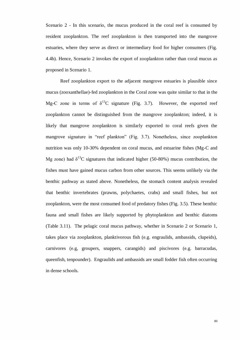
80

Scenario 2 - In this scenario, the mucus produced in the coral reef is consumed by

resident zooplankton. The reef zooplankton is then transported into the mangrove

estuaries, where they serve as direct or intermediary food for higher consumers (Fig.

4.4b). Hence, Scenario 2 invokes the export of zooplankton rather than coral mucus as

proposed in Scenario 1.

Reef zooplankton export to the adjacent mangrove estuaries is plausible since

mucus (zooxanthellae)-fed zooplankton in the Coral zone was quite similar to that in the

Mg-C zone in terms of δ13

C signature (Fig. 3.7). However, the exported reef

zooplankton cannot be distinguished from the mangrove zooplankton; indeed, it is

likely that mangrove zooplankton is similarly exported to coral reefs given the

mangrove signature in “reef plankton” (Fig. 3.7). Nonetheless, since zooplankton

nutrition was only 10-30% dependent on coral mucus, and estuarine fishes (Mg-C and

Mg zone) had δ13

C signatures that indicated higher (50-80%) mucus contribution, the

fishes must have gained mucus carbon from other sources. This seems unlikely via the

benthic pathway as stated above. Nonetheless, the stomach content analysis revealed

that benthic invertebrates (prawns, polychaetes, crabs) and small fishes, but not

zooplankton, were the most consumed food of predatory fishes (Fig. 3.5). These benthic

fauna and small fishes are likely supported by phytoplankton and benthic diatoms

(Table 3.11). The pelagic coral mucus pathway, whether in Scenario 2 or Scenario 1,

takes place via zooplankton, planktivorous fish (e.g. engraulids, ambassids, clupeids),

carnivores (e.g, groupers, snappers, carangids) and piscivores (e.g. barracudas,

queenfish, tenpounder). Engraulids and ambassids are small fodder fish often occurring

in dense schools.

81

Scenario 3 - Unlike Scenario 1 and 2, which invoke the outwelling of mucus or mucus-

fed zooplankton from reef to mangrove, Scenario 3 explains zooxanthellae contribution

by fish movements between coral reef and mangrove estuaries (Fig. 4.4c).

Movements of fish feeding in the reef area and then into the mangrove area, and

vice versa, can explain the strong δ13

C signature of zooxanthellae in both reef and

mangrove fishes (Fig. 3.8), which cannot be fully explained in Scenario 1 and 2. Mucus

or zooplankton drift alone cannot account for the much higher contribution of

zooxanthellae carbon in most fishes since few species are zooplankton feeders. Scenario

3 assumes that fishes in the reef feed directly on zooxanthellae and/or coral mucus, or

indirectly, that fauna that feeds on zooxanthellae or mucus. This scenario appears to be

feasible given the δ13

C values of fish species and the evidence that such species were

found in both reef and mangrove; these included 31 species or 40% of the 77 fish

species listed in Table 3.13, e.g. grey mullets such as Valamugil buchanani, the

pickhandle barracuda, Sphyraeno jello, the talang queenfish, Scomberoides

commersonianus, the yellowtail fusilier Caesio cunning, and the bigeye trevally,

Caranx sexfasciatus. However, some species are known to exhibit ontogenetic

migration between reef and mangrove, e.g. Russell’s snapper, Lutjanus russelli

(Sheaves, 1995), John’s snapper L. johnii (Tanaka et al., 2011) and the orange-spotted

grouper, Epinephelus coioides (Sheaves, 1995).

82

Figure 4.4: Diagrammatic representation of three possible scenarios of energy transfer from coral reef

(Coral) to the adjacent mangrove (Mg + Up). (a) Scenario 1: coral mucus is outwelled into mangrove by

currents and consumed by mangrove zooplankton and fishes; (b) Scenario 2: coral mucus is consumed by

reef zooplankton before they are advected into mangrove and consumed by fishes. (3) Scenario 3: coral

reef fishes feed on either coral mucus or/and zooplankton, migrate into mangroves and vice versa.

83

4.6 Limitations of present study and suggestions for future research

1) Sampling methods did not successfully sample, for each species, fish of

adequate size range (small and big). This possibly indicates that the gill nets

(mesh sizes are 1 inch and 2 inches) used were not able to sample all life history

stages of fishes in the corals and mangroves. Hence, the nursery ground value of

both corals and mangroves to fishes could not be determined.

2) The gill nets could not sample adequately the benthic and demersal fish.

Some may be caught by the fish pots. Hence, this study largely missed the

demersal or benthic species as well as not being able to quantify fish abundance.

Therefore, the species richness for both habitats is likely underestimated even

with data from previous studies. A more quantitative fishing method was not

used because fishing gears such as trawl nets is unavailable on the island.

3) This study has alluded to the major contribution of coral zooxanthellae as

primary producer in the study area, and that outwelled coral mucus or/and

zooplankton that feed on it, fuel the adjacent mangrove waters based on stable

isotope analysis. Unfortunately, the study did not sample the drifted mucus flocs

to show the connectivity directly. The study was also unable to obtain the δ13

C

signature of coral mucus. Future studies employing superior techniques and

methods of study are required to test the derived hypothesis.

4) It would be more informative and beneficial if the trophic pathway from

primary sources could be traced via the various trophic levels. This study did not

84

include the many invertebrates consumed by the fish (from stomach content

analysis) in the SIA, such as prawns, crabs and polychaetes, which are likely the

trophic intermediaries. This limitation was due to the lack of suitable gears as

well as the limited duration of the study.

5) Although this study attempted to at least sample the copepod fauna (major

zooplankton) for SIA, and to link them to their potential food of coral mucus and

phytoplankton, it did not attempt to sample and sort the other zooplankton fauna

due to time constraints. A more comprehensive sampling and analysis of other

zooplankton would be beneficial in future studies.

85

5.0 CONCLUSION

The fish communities of Langkawi’s northeastern coral reefs and mangroves

have a relatively high number of common (similar) species. Despite turbid waters due to

the island’s rapid development, the nearshore coral reefs still display relatively high

habitat complexity. These coral reefs coupled to the adjacent mainland mangroves offer

a suitable refuge, feeding and habitat space for marine fishes.

One major finding is that coral zooxanthellae and phytoplankton are the two

primary food sources in the coupled coastal biotopes. Based on stable isotope analysis,

outwelled coral mucus and zooplankton are hypothesized to be the vehicles of transfer

of source energy from coral zooxanthellae to fish consumers. However, the study has

put forward three possible scenarios of habitat connectivity involving not only the

transport of mucus and zooplankton, but also fish movements. Thus, the present

findings support the two hypotheses of ecological connectivity set up in the study.

This study has provided important information for the management of

Langkawi’s northeastern coral reefs and mangroves in general, and Kilim Geoforest

Park in particular. The study suggests that a comprehensive integrated management

strategy or plan should be instituted immediately in view of the fast developing tourism

industry, which has given impetus to the island’s rapid development, in order to protect

the health and function of the remaining mangroves and coral reef ecosystems of

Langkawi island.

86

REFERENCES

Abrantes, K., & Sheaves, M. (2009). Food web structure in a near-pristine mangrove

area of the Australian Wet Tropics. Estuarine, Coastal and Shelf Science, 82(4),

597–607.

Affendi, Y. A. (2005). Coral reefs of North East Pulau Langkawi. Malaysian Journal of

Science, 24, 145 – 158.

Alamaru, A., Loya, Y., Brokovich, E., Yam, R., & Shemesh, A. (2009). Carbon and

nitrogen utilization in two species of Red Sea corals along a depth gradient:

Insights from stable isotope analysis of total organic material and lipids.

Geochimica et Cosmochimica Acta, 73(18), 5333–5342.

Alongi, D. M. (2002). Present state and future of the world’s mangrove forests.

Environmental Conservation, 29, 331 - 349

Alongi, D. M. (2008). Mangrove forests: Resilience, protection from tsunamis, and

responses to global climate change. Estuarine, Coastal and Shelf Science, 76(1), 1–

13.

Alongi, D. M. (2009). The Energetics of Mangrove Forests. (p. 216).

Anthony, K. R. N., & Larcombe, P. (2000). Coral reefs in turbid waters: sediment-

induced stresses in corals and likely mechanisms of adaptation. In 9th

International Coral Reef Symposium (p. 6).

Baker, R., & Sheaves, M. (2005). Redefining the piscivore assemblage of shallow

estuarine nursery habitats. Marine Ecology Progress Series, 291, 197–213.

Benfield, M. C., & Minello, T. J. (1996). Relative effects of turbidity and light intensity

on reactive distance and feeding of an estuarine fish. Environmental Biology of

Fishes, 46(2), 211–216.

Benson, A. A., & Muscatine, L. (1974). Wax in coral mucus : Energy transfer from

corals to reef fishes. Limnology and Oceanography, 19(5), 810–814.

Beukers-Stewart, B., & Jones, G. (2004). The influence of prey abundance on the

feeding ecology of two piscivorous species of coral reef fish. Journal of

Experimental Marine Biology and Ecology, 299, 155–184.

Birkeland, C. (1997). Life and Death of Coral Reefs (p. 536). New York: Chapman &

Hall.

Bouillon, S., Connolly, R. M., & Lee, S. Y. (2008). Organic matter exchange and

cycling in mangrove ecosystems: Recent insights from stable isotope studies.

Journal of Sea Research, 59(1-2), 44–58.

Bouillon, S., Mohan, P. C., Sreenivas, N., & Dehairs, F. (2000). Sources of suspended

organic matter and selective feeding by zooplankton in an estuarine mangrove

87

ecosystem as traced by stable isotopes. Marine Ecology Progress Series, 208, 79–

92.

Burke, L., Reytar, K., Spalding, M., & Perry, A. (2011). Reefs at Risk Revisited.

Defenders (Vol. 74, p. 114).

Burke, L., Selig, E., & Spalding, M. (2002). Reefs at risk in Southeast Asia. World

Fishing (p. 72). World Resources Institute Washington, DC.

Caley, M. J., & St John, J. (1996). Refuge availability structures assemblages of tropical

reef fishes. Journal of Animal Ecology, 65(4), 414–428.

Chew, L. L., Chong, V. C., Tanaka, K., & Sasekumar, A. (2012). Phytoplankton fuel

the energy flow from zooplankton to small nekton in turbid mangrove waters.

Marine Ecology Progress Series, 469, 7–24.

Chittaro, P. M., Usseglio, P., & Sale, P. F. (2005). Variation in fish density, assemblage

composition and relative rates of predation among mangrove, seagrass and coral

reef habitats. Environmental Biology of Fishes, 72(2), 175–187.

Chong, V. C. (2007a). Importance of coastal habitats in sustaining the fisheries industry.

In P. E. Chee, M. N. Devakie, I. Ismail, A. L. Faazaz, N. Ahmad Adnan, D. R.

Shahuntala, & A. R. Masazurah (Eds.), Proceedings of the 4th National Fisheries

Symposium (pp. 113–137). Penang: Fisheries Research Institute.

Chong, V. C. (2007b). Mangroves-fisheries linkages - the Malaysian perspective.

Bulletin of Marine Science, 80(3), 755–772.

Chong, V. C., Lee, P. K. Y., & Lau, C. M. (2010). Diversity, extinction risk and

conservation of Malaysian fishes. Journal of Fish Biology, 76(9), 2009–66.

Chong, V. C., Affendy, N., Ooi, A. L., & Chew, L. L. (2005). The fishes and

invertebrates of mangrove estuaries in Northeastern Langkawi Island. Malayan

Nature Journal, 57(2), 193–208.

Chong, V. C., Ng, Y. P., Hairi, B. J., Ooi, A. L., Chew, L. L., Amirah, M., & Affendy,

N. (2005). Update of the fishes of mangrove and coastal waters of Northeastern

Langkawi. Malaysian Journal of Science, 24, 167–184.

Cocheret de la Morinière, E., Nagelkerken, I., van der Meij, H., & van der Velde, G.

(2004). What attracts juvenile coral reef fish to mangroves: habitat complexity or

shade? Marine Biology, 144(1), 139–145.

Cocheret de la Morinière, E., Pollux, B. J. A., Nagelkerken, I., Hemminga, M. A.,

Huiskes, A. H. L., & van der Velde, G. (2003). Ontogenetic dietary changes of

coral reef fishes in the mangrove-seagrass-reef continuum : stable isotopes and gut-

content analysis. Marine Ecology Progress Series, 246, 279–289.

Cole, A. J., Pratchett, M. S., & Jones, G. P. (2008). Diversity and functional importance

of coral-feeding fishes on tropical coral reefs. Fish and Fisheries, 9, 286–307.

88

Coles, S. L., & Strathmann, R. (1973). Observations on coral mucus “flocs” and their

potential trophic significance. Limnology and Oceanography, 18, 673–678.

Crossland, C. J., Barnes, D. J., & Borowitzka, M. a. (1980). Diurnal lipid and mucus

production in the staghorn coral Acropora acuminata. Marine Biology, 60(2-3),

81–90.

Cyrus, D., & Blaber, S. (1987). The influence of turbidity on juvenile marine fish in the

estuaries of Natal, South Africa. Continental Shelf Research, 7, 1411–1416.

Davies, P. S. (1984). The role of zooxanthellae in the nutritional energy requirements of

Pocillopora eydouxi. Coral Reefs, (2), 181–186.

De Bruin, G. H. P., Russel, B. C., & Bogusch, A. (1994). The marine fisheries

resources of Sri Lanka. In FAO Species Scientific Field Guide for Fishery

Purposes. Rome.

Dominici-Arosemena, A., & Wolff, M. (2005). Reef fish community structure in Bocas

del Toro (Caribbean, Panama): Gradients in habitat complexity and exposure.

Caribbean Journal of Science, 41(3), 613–637.

Dorenbosch, M. (2006). Connectivity Between Fish Assemblages of Seagrass Beds,

Mangroves and Coral Reefs: Evidence from the Caribbean and the western Indian

Ocean. (Doctoral dissertation, Radboud University Nijmegen, The Netherlands).

Retrieved from https://repository.ubn.kun.nl/bitstream/2066/27459/1/27459.pdf

Dorenbosch, M., Grol, M. G. G., Christianen, M., Nagelkerken, I., & van der Velde, G.

(2005). Indo-Pacific seagrass beds and mangroves contribute to fish density and

diversity on adjacent coral reefs. Marine Ecology Progress Series, 302, 63–76.

Dorenbosch, M., van Riel, M. C., Nagelkerken, I., & van der Velde, G. (2004). The

relationship of reef fish densities to the proximity of mangrove and seagrass

nurseries. Estuarine, Coastal and Shelf Science, 60(1), 37–48.

Drazen, J. C., Popp, B. N., Choy, C. A., Clemente, T., De Forest, L., & Smith, K. L. J.

(2008). Bypassing the abyssal benthic food web: Macrourid diet in the eastern

North Pacific inferred from stomach content and stable isotopes analyses.

Limnology and Oceanography, 53(6), 2644–2654

Ducklow, H. W., & Mitchell, R. (1979). Composition of mucus released by coral reef

coelenterates. Limnology and Oceanography, 24(4), 706–714.

Edinger, E. N., & Risk, M. J. (2000). Reef classification by coral morphology predicts

coral reef conservation value. Biological Conservation, 92, 1–13.

English, S., Wilkinson, C., & Baker, V. (1997). Line Intercept Transect. In Survey

Manual for Tropical Marine Resources. Townsville.

Fishcher, W., & Whitehead, P. J. P. (Eds.). (1974). FAO species identification sheets for

fisheries purposes. Eastern Indian Ocean and Western Central Pacific, Volume 1 –

4. Rome: FAO.

89

Froese, R., & Pauly, D. (2012). FishBase. World Wide Web electronic publication.

Retrieved from www.fishbase.org

Giesen, W., Wulffraat, S., Zieren, M., & Scholten, L. (2006). Mangrove Guidebook For

Southeast Asia (p. 186).

Gillanders, B. M., Able, K. W., Brown, J. A., Eggleston, D. B., & Sheridan, P. F.

(2003). Evidence of connectivity between juvenile and adult habitats for mobile

marine fauna: an important component of nurseries. Marine Ecology Progress

Series, 247, 281–295.

Glenda, N., Azhar, H., Chong, V. C., & Phang, S. M. (2005). The scientific, social,

environmental and economic value of N.E. Langkawi: an overview of the present

status. Malaysian Journal of Science, 24, 219–235.

Glynn, P. W. (1997). Bioerosion and Coral-Reef Growth: A Dynamic Balance. In C.

Birkeland (Ed.), Life and Death of Coral Reefs (pp. 68–95). Chapman & Hall.

Glynn, P. W., Stewart, R. H., & McCosker, J. E. (1972). Pacific Coral Reefs of Panama:

Structure, distribution and predators. Geologische Rundschau, 61(2), 483–519.

Gomez, E. D., Alino, P. M., Yap, H. T., & Licuanan, W. Y. (1994). A review of the

status of Philippine reefs. Marine Pollution Bulletin, 29(94), 62–68.

Gratwicke, B., & Speight, M. R. (2005). The relationship between fish species richness,

abundance and habitat complexity in a range of shallow tropical marine habitats.

Journal of Fish Biology, (66), 650–667.

Grol, M. G. G., Nagelkerken, I., Rypel, A. L., & Layman, C. A. (2011). Simple

ecological trade-offs give rise to emergent cross-ecosystem distributions of a coral

reef fish. Oecologia, 165(1), 79–88.

Hajisamae, S., Chou, L. M., & Ibrahim, S. (2004). Feeding habits and trophic

relationships of fishes utilizing an impacted coastal habitat, Singapore.

Hydrobiologia, 520, 61–71.

Hobson, K. A., & Wassenaar, L. I. (1999). Stable isotope ecology: an introduction.

Oecologia, 120(3), 312–313.

Hoegh-Guldberg, O., Hoegh-Guldberg, H., Veron, J. E. N., Green, A., Gomez, E. D.,

Lough, J., … Oliver, J. (2009). The Coral Triangle and Climate Change:

Ecosystems, People and Societies at Risk (p. 276). Brisbane.

Hoeksema, B. (2007). Delineation of the Indo-Malayan centre of maximum marine

biodiversity: the Coral Triangle. In W. Renema (Ed.), Biogeography, Time, and

Place: Distributions, Barriers, and Islands (pp. 117–178). Springer.

Hogarth, P. J. (2007). The Biology of Mangroves and Seagrasses (p. 272). Oxford

University Press.

90

Honda, K., Nakamura, Y., Nakaoka, M., Uy, W. H., & Fortes, M. D. (2013). Habitat

use by fishes in coral reefs, seagrass beds and mangrove habitats in the Philippines.

PloS One, 8(8), 10.

Hubbard, J. A. E. B., & Pocock, Y. P. (1972). Sediment rejection by recent scleractinian

corals: a key to palaeo-environmental reconstruction. Geologische Rundschau, 61,

598–626.

Huxham, M., Kimani, E., & Augley, J. (2004). Mangrove fish: a comparison of

community structure between forested and cleared habitats. Estuarine, Coastal and

Shelf Science, 60(4), 637–647.

Hyslop, E. J. (1980). Stomach contents analysis-a review of methods and their

application. Journal of Fish Biology, 17(4), 411–429.

Jalal, K. C. A., Faizul, H. N. N., Kamaruzzaman, B. Y., Shahbudin, S., Alam, M. Z., &

Irwandi, J. (2009). Studies on physico-chemical characteristics and sediment

environment along the coastal waters in Pulau Tuba, Langkawi, Malaysia. Aquatic

Ecosystem Health & Management, 12(4), 350–357.

Jaxion-Harm, J., Saunders, J., & Speight, M. R. (2012). Distribution of fish in seagrass,

mangroves and coral reefs: life-stage dependent habitat use in Honduras. Rev. Biol.

Trop, 60(June), 683–698.

Johannes, R. E. (1967). Ecology of organic aggregates in the vicinity of a coral reef.

Limnology and Oceanography, 12(2), 189–195.

Jones, D. L., Walter, J. F., Brooks, E. N., & Serafy, J. E. (2010). Connectivity through

ontogeny: fish population linkages among mangrove and coral reef habitats.

Marine Ecology Progress Series, 401, 245–258.

Kanou, K., & Sano, M. (2004). Food habits of fishes on unvegetated tidal mudflats in

Tokyo Bay, central Japan. Fisheries Science, 70, 978–987.

Kelley, R. A. (2009). Indo Pacific Coral Finder. Townsville: BYOGUIDES

Kelley, R., & Ryan, G. (2000). Crossing the Blue Highway. Australia: Australian Coral

Reef Society.

Kerry, J. T., & Bellwood, D. R. (2011). The effect of coral morphology on shelter

selection by coral reef fishes. Coral Reefs, 415–424.

Kimura, S., Satapoomin, U., & Matsuura, K. (Eds.). (2009). Fishes of Andaman Sea,

west coast of southern Thailand (p. vi+346). Tokyo: National Museum of Nature

and Science, Tokyo.

Kleypas, J. A., McManus, J. W., & Menez, L. A. B. (1999). Environmental limits to

coral reef development : Where do we draw the line? American Zoologist, 39, 146–

159.

Kneib, R. T. (2002). Salt marsh ecoscapes and production transfers by estuarine nekton

in the southeastern United States. In M. P. Weinstein & D. A. Kreeger (Eds.),

91

Concepts and Controversies in Tidal Marsh Ecology (pp. 267–291). New York,

Boston, Dordrecht, London, Moscow: Kluwer Academic Publishers.

Laegdsgaard, P., & Johnson, C. (2001). Why do juvenile fish utilise mangrove habitats?

Journal of Experimental Marine Biology and Ecology, 257(2), 229–253.

Larcombe, P., Costen, A., & Woolfe, K. J. (2001). The hydrodynamic and sedimentary

setting of nearshore coral reefs, central Great Barrier Reef shelf, Australia: Paluma

Shoals, a case study. Sedimentology, 48(4), 811–835.

Larcombe, P., & Woofle, K. J. (1999). Increased sediment supply to the Great Barrier

Reef will not increase sediment accumulation at most coral reefs. Coral Reefs,

(18), 163–169.

Laroche, J., Baran, E., & Rasoanandrasana, N. (1997). Temporal patterns in a fish

assemblage of a semiarid mangrove zone in Madagascar. Journal of Fish Biology,

51(1), 3–20.

Liu, J. (1997). Morphological comparison of the feeding apparatus of three co-occurring

species of ponyfishes (Leiognathidae). Chinese Journal of Oceanology and

Limnology, 15(3), 224–226.

Lugendo, B. R., Nagelkerken, I., Jiddawi, N., Mgaya, Y. D., & van der Velde, G.

(2007). Fish community composition of a tropical nonestuarine embayment in

Zanzibar, Tanzania. Fisheries Research, 73, 1213–1223.

Lugendo, B. R., Nagelkerken, I., van der Velde, G., & Mgaya, Y. D. (2006). The

importance of mangroves , mud and sand flats , and seagrass beds as feeding areas

for juvenile fishes in Chwaka Bay , Zanzibar : gut content and stable isotope

analyses. Journal of Fish Biology, 69, 1639–1661.

Marguillier, S., van der Velde, G., Dehairs, F., Hemminga, M. A., & Rajagopal, S.

(1997). Trophic relationships in an interlinked mangrove-seagrass ecosystem as

traced by δ13

C and δ15

N. Marine Ecology Progress Series, 151, 115–121.

Marshall, N. (1965). Detritus over the reef and its potential contribution to adjacent

waters of Eniwetok Atoll. Ecology, 46(3), 343–344.

Maugé, L. A. (1986). Gobiidae. In J. Daget, J. P. Gosse, & D. F. E. Thys van

denAudenaerde (Eds.), Check-list of the freshwater fishes of Africa (CLOFFA) (pp.

358–388). Brussels; Tervuren; Paris: ISNB; MRAC; ORSTOM. Retrieved from

http://www.fishbase.org/summary/Acentrogobius-caninus.html

McCook, L. J., Almany, G. R., Berumen, M. L., Day, J. C., Green, A. L., Jones, G. P.,

… Thorrold, S. R. (2009). Management under uncertainty: guide-lines for

incorporating connectivity into the protection of coral reefs. Coral Reefs, 28(2),

353–366.

McCutchan, J. H. J., Lewis, W. M. K., & McGrath, C. C. (2003). Variation in trophic

shift for stable isotope ratios of carbon, nitrogen, and sulfur. Oikos, 102(2), 378–

390.

92

Meikle, P., Richards, G. N., & Yellowlees, D. (1988). Structural investigations on the

mucus from six species of coral. Marine Biology, 99, 187–193.

Minagawa, M., & Wada, E. (1984). Stepwise enrichment of 15

N along food chains:

Further evidence and the relation between δ15

N and animal age. Geochimica et

Cosmochimica Acta, 48, 1135–1140.

Moberg, F., & Folke, C. (1999). Ecological goods and services of coral reef ecosystems.

Ecological Economics, 29(2), 215–233.

Moberg, F., Nyström, M., Kautsky, N., Tedengren, M., & Jarayabhand, P. (1997).

Effects of reduced salinity on the rates of photosynthesis and respiration in the

hermatypic corals Porites lutea and Pocillopora damicornis. Marine Ecology

Progress Series, 157, 53–59.

Mohsin, A. K. M., & Ambak, M. A. (1996). Marine Fishes and Fisheries of Malaysia

and Neighbouring Countries. Serdang: University Pertanian Press.

Mooney, H. A., Cropper, A., Capistrano, D., Carpenter, S. R., Chopra, K., Dasgupta, P.,

… Zhao, S. (2005). Ecosystems and Human Well-Being: Wetlands and Water

Synthesis : A Report of the Millennium Ecosystem Assessment. (J. Sarukhan & A.

Whyte, Eds.) (p. 68). Washington, DC.: World Resources Institute.

MPP-EAS. (1999). Total economic valuation: coastal and marine resources in the

Straits of Malacca (p. 52). Quezon City, the Philippines.

Muller-Parker, G., & D’Elia, C. F. (1997). Interactions Between Corals and Their

Symbiotic Algae. In Life and Death of Coral Reefs (pp. 96–113). New York:

Chapman & Hall.

Mumby, P. J., Edwards, A. J., Ernesto Arias-Gonzalez, J., Lindeman, K. C., Blackwell,

P. G., Gall, A., … Llewellyn, G. (2004). Mangroves enhance the biomass of coral

reef fish communities in the Caribbean. Journal of Geophysical Research,

108(B5), 533–536.

Mumby, P. J., & Hastings, A. (2008). The impact of ecosystem connectivity on coral

reef resilience. Journal of Applied Ecology, 45(3), 854–862.

Munroe, T. A. (2001). Cynoglossidae. In K. E. Carpenter & V. H. Niem (Eds.), FAO

species identification guide for fishery purposes. The living marine resources of

the Western Central Pacific. Volume 6. Bony fishes part 4 (Labridae to

Latimeriidae), estuarine crocodiles, sea turtles, sea snakes and marine mammals

(pp. 3381–4218). Rome: FAO.

Muscatine, L., McCloskey, L. R., & Marian, R. E. (1981). Estimating the daily

contribution of carbon from zooxanthellae to coral animal respiration. Limnology

and Oceanography, 26(4), 601–611.

Muscatine, L., Porter, J. W., & Kaplan, I. R. (1989). Resource partitioning by reef

corals as determined from stable isotope composition I. δ13

C of zooxanthellae and

animal tissue vs depth. Marine Biology, 193(100), 185 – 193.

93

Nagelkerken, I. (2007). Are non-estuarine mangroves connected to coral reefs through

fish migration? Bulletin of Marine Science, 80(3), 595–607.

Nagelkerken, I. (Ed.). (2009a). Ecological Connectivity among Tropical Coastal

Ecosystems (p. 615). Springer Science+Business Media.

Nagelkerken, I. (2009b). Evaluation of nursery function of mangroves and seagrass

beds for tropical decapods and reef fishes: Patterns and underlying mechanisms. In

I. Nagelkerken (Ed.), Ecological Connectivity among Tropical Coastal Ecosystems

(pp. 357 – 399). Springer Science+Business Media.

Nagelkerken, I., Blaber, S. J. M., Bouillon, S., Green, P., Haywood, M., Kirton, L. G.,

… Somerfield, P. J. (2008). The habitat function of mangroves for terrestrial and

marine fauna: A review. Aquatic Botany, 89(2), 155–185.

Nagelkerken, I., De Schryver, A. M., Verweij, M. C., Dahdouh-Guebas, F., van der

Velde, G., & Koedam, N. (2010). Differences in root architecture influence

attraction of fishes to mangroves: A field experiment mimicking roots of different

length, orientation, and complexity. Journal of Experimental Marine Biology and

Ecology, 396(1), 27–34.

Nagelkerken, I., Dorenbosch, M., Verberk, W., Cocheret de la Morinière, E., & van der

Velde, G. (2000). Importance of shallow-water biotopes of a Caribbean bay for

juvenile coral reef fishes: patterns in biotope association, community structure and

spatial distribution. Marine Ecology Progress Series, 202, 175–192.

Nagelkerken, I., & van der Velde, G. (2002). Do non-estuarine mangroves harbour

higher densities of juvenile fish than adjacent shallow-water and coral reef habitats

in Curacao (Netherlands Antilles)? Marine Ecology Progress Series, 245, 191–

204.

Nagelkerken, I., & van der Velde, G. (2004a). Are Caribbean mangroves important

feeding grounds for juvenile reef fish from adjacent seagrass beds? Marine

Ecology Progress Series, 274, 143–151.

Nagelkerken, I., & van der Velde, G. (2004b). Relative importance of interlinked

mangroves and seagrass beds as feeding habitats for juvenile reef fish on a

Caribbean island. Marine Ecology Progress Series, 274, 153–159.

Nagelkerken, I., van der Velde, G., Gorissen, M. W., Meijer, G. J., Van’t Hof, T., & den

Hartog, C. (2000). Importance of mangroves, seagrass beds and the shallow coral

reef as a nursery for important coral reef fishes, using a visual census technique.

Estuarine, Coastal and Shelf Science, 51(1), 31–44.

Nakamura, Y., Horinouchi, M., Shibuno, T., Tanaka, Y., Miyajima, T., Koike, I., …

Sano, M. (2008). Evidence of ontogenetic migration from mangroves to coral reefs

by black-tail snapper Lutjanus fulvus: stable isotope approach. Marine Ecology

Progress Series, 355(2001), 257–266.

Nakamura, Y., Kawasaki, H., & Sano, M. (2007). Experimental analysis of recruitment

patterns of coral reef fishes in seagrass beds: Effects of substrate type, shape, and

rigidity. Estuarine, Coastal and Shelf Science, 71(3-4), 559–568.

94

Nanjo, K., Kohno, H., & Sano, M. (2008). Food habits of fishes in the mangrove

estuary of Urauchi River, Iriomote Island, southern Japan. Fisheries Science, 74,

1024–1033.

Naumann, M. S., Mayr, C., Struck, U., & Wild, C. (2010). Coral mucus stable isotope

composition and labeling: experimental evidence for mucus uptake by epizoic

acoelomorph worms. Marine Biology, 157(11), 2521–2531.

Naumann, M. S., Richter, C., el-Zibdah, M., & Wild, C. (2009). Coral mucus as an

efficient trap for picoplanktonic cyanobacteria–implications for pelagic–benthic

coupling in the reef ecosystem. Marine Ecology Progress Series, 385, 65–76.

Nyunja, J., Ntiba, M., Onyari, J., Mavuti, K., Soetaert, K., & Bouillon, S. (2009).

Carbon sources supporting a diverse fish community in a tropical coastal

ecosystem (Gazi Bay, Kenya). Estuarine, Coastal and Shelf Science, 83(3), 333–

341.

Ogden, J. C., & Gladfelter, E. H. (1983). Coral reefs, seagrass beds and mangroves:

Their interaction in the coastal zones of the Caribbean (p. 133). St. Croix.

Okamura, K., Tanaka, K., Siow, R., Man, A., Kodama, M., & Ichikawa, T. (2010).

Spring tide hypoxia with relation to chemical properties of the sediments in the

Matang Mangrove Estuary, Malaysia. Japan Agricultural Research Quarterly:

JARQ, 44(3), 325–333.

Olin, M., Malinen, T., & Ruuhijärvi, J. (2009). Gillnet catch in estimating the density

and structure of fish community—Comparison of gillnet and trawl samples in a

eutrophic lake. Fisheries Research, 96(1), 88–94.

Parnell, A. C., Inger, R., Bearhop, S., & Jackson, A. L. (2010). Source partitioning

using stable isotopes: coping with too much variation. PloS One, 5(3), 5.

Peterson, B. J., & Fry, B. (1987). Stable isotopes in ecosystem studies. Annual Review

of Ecology and Systematics, 18(1), 293–320.

Polis, G. A. (1994). Food webs, trophic cascades and community structure. Australian

Journal of Ecology, 19, 121–136.

Post, D. M. (2002). Using stable isotopes to estimate trophic position: models, methods,

and assumptions. Ecology, 83(3), 703–718.

Raje, S. G. (1993). Some aspects of biology of Alepes djedaba (Forsskal) from Veraval,

Gujarat. Indian Journal of Fisheries, 40(3), 189 – 192.

Rau, G. H., Knauss, K. G., Langer, W. H., & Caldeira, K. (2007). Reducing energy-

related CO2 emissions using accelerated weathering of limestone. Energy, 32(8),

1471–1477.

Reid, D. D. J., Quinn, G. P. G., Lake, P. S. P., & Reich, P. (2008). Terrestrial detritus

supports the food webs in lowland intermittent streams of south-eastern Australia:

a stable isotope study. Freshwater Biology, 53(10), 2036–2050.

95

Richman, S., Loya, Y., & Slobodkin, L. B. (1975). The rate of mucus production by

corals and its assimilation by the coral reef copepod Acartia negligens. Limnology

and Oceanography, 20(November), 918–923.

Roberts, C. M., & Ormond, R. F. G. (1987). Habitat complexity and coral reef fish

diversity and abundance on Red Sea fringing reefs. Marine Ecology Progress

Series, 41(1972), 1–8.

Rogers, C. S. (1990). Responses of coral reefs and reef organisms to sedimentation.

Marine Ecology Progress Series, 62, 185–202.

Rotherham, D., Johnson, D. D., Kesby, C. L., & Gray, C. A. (2012). Sampling estuarine

fish and invertebrates with a beam trawl provides a different picture of populations

and assemblages than multi-mesh gillnets. Fisheries Research, 123-124, 49–55.

Sale, P. F., Van Lavieren, H., Ablan Lagman, M. C., Atema, J., Butler, M., Fauvelot, C.,

… Stewart, H. L. (2010). Preserving Reef Connectivity: A Handbook for Marine

Protected Area Managers. (L. Benedetti, Ed.) Management (p. 79). Connectivity

Working Group, Coral Reef Targeted Research & Capacity Building for

Management Program, UNU-INWEH.

Salini, J. P., Blaber, S. J. M., & Brewer, D. T. (1994). Diets of Trawled Predatory Fish

of the Gulf of Carpentaria, Australia, with Particular Reference to Predation on

Prawns. Australian Journal of Marine and Freshwater Research, 45, 397–411.

Sasaki, K. (2001). Sciaenidae. In K. E. Carpenter & V. H. Niem (Eds.), FAO species

identification guide for fishery purposes. The living marine resources of the

Western Central Pacific. Volume 5. Bony fishes part 3 (Menidae to

Pomacentridae) (pp. 2791–3380). Rome: FAO.

Sasekumar, A., & Ooi, A. L. (2005). Fauna of Langkawi Mangrove Forests. Malaysian

Journal of Science, 24, 123–132.

Schuhmacher, H. (1977). Ability in fungiid corals to overcome sedimentation. In

Proceedings of the 3rd International Coral Reef Symposium. Miami, Florida.

Shahbudin, S., Zuhairi, A., & Kamaruzzaman, B. Y. (2012). Impact of coastal

development on mangrove cover in Kilim river, Langkawi Island, Malaysia.

Journal of Forestry Research, 23(2), 185–190.

Sheaves, M. (1995). Large lutjanid and serranid fishes in tropical estuaries: Are they

adults or juveniles? Marine Ecology Progress Series, 129, 31–41.

Sheaves, M. (2005). Nature and consequences of biological connectivity in mangrove

systems. Marine Ecology Progress Series, 302, 293–305.

Sheaves, M. (2009). Consequences of ecological connectivity: the coastal ecosystem

mosaic. Marine Ecology Progress Series, 391, 107–115.

Sheppard, C. R. C., Davy, S. K., & Pilling, G. M. (2009). The Biology of Coral Reefs (p.

339). Oxford University Press.

96

Shinnaka, T., Sano, M., Ikejima, K., Tongnunui, P., Horinouchi, M., & Kurokura, H.

(2007). Effects of mangrove deforestation on fish assemblage at Pak Phanang Bay,

southern Thailand. Fisheries Science, 73(4), 862–870.

Smith-Vaniz, W. F. (1999). Carangidae. In K. E. Carpenter & V. H. Niem (Eds.), FAO

species identification guide for fishery purposes. The living marine resources of

the Western Central Pacific. Volume 4. Bony fishes part 2 (Mugilidae to

Carangidae) (pp. 2069–2790). Rome: FAO.

Sorokin, Y. I. (1993). Coral reef ecology (p. 465). Berlin: Springer-Verlag.

Tanaka, K., Hanamura, Y., Chong, V. C., Watanabe, S., Man, A., Mohd Kassim, F., …

Ichikawa, T. (2011). Stable isotope analysis reveals ontogenetic migration and the

importance of a large mangrove estuary as a feeding ground for juvenile John’s

snapper Lutjanus johnii. Fisheries Science, 77(5), 809–816.

Then, A. Y. H. (2009). The structure and trophodynamics of the fish community in

estuaries of Matang Mangrove Forest Reserve, Peninsular Malaysia.

(Unpublished Master’s Thesis) University of Malaya, Kuala Lumpur.

Thollot, & Thollot, P. (1992). Importance of mangroves for Pacific reef fish species,

myth or reality. In Proceedings of the 7th International Coral Reef Symposium

(Vol. 2, pp. 934–941).

Thom, B. G. (1984). Coastal landforms and geomorphic processes. In S. C. Snedaker &

J. G. Snedaker (Eds.), The Mangrove Ecosystem: Research Methods (pp. 3–17).

Paris: UNESCO.

Tremblay, P., Grover, R., Maguer, J. F., Legendre, L., & Ferrier-Pagès, C. (2012).

Autotrophic carbon budget in coral tissue: a new 13

C-based model of photosynthate

translocation. Journal of Experimental Biology, (215), 1384–1393.

Unsworth, R. K. F., De León, P. S., Garrard, S. L., Jompa, J., Smith, D. J., & Bell, J. J.

(2008). High connectivity of Indo-Pacific seagrass fish assemblages with

mangrove and coral reef habitats. Marine Ecology Progress Series, 353, 213–224.

Vander Zanden, M., & Rasmussen, J. (2001). Variation in δ15

N and δ13

C trophic

fractionation: Implications for aquatic food web studies. Limnology and

Oceanography, 46(8), 2061–2066.

Veron, J. E. N., Devantier, L. M., Turak, E., Green, A. L., Kininmonth, S., Stafford-

Smith, M. G., & Peterson, N. (2009). Delineating the Coral Triangle. Galaxea,

Journal of Coral Reef Studies, 11, 91–100.

Veron, J. E. N., Hoegh-Guldberg, O., Lenton, T. M., Lough, J. M., Obura, D. O.,

Pearce-Kelly, P., … Rogers, a D. (2009). The coral reef crisis: The critical

importance of 350 ppm CO2. Marine Pollution Bulletin, 58(10), 1428–36.

Veron, J. E. N., & Stafford-Smith, M. G. (2000). Coral ID. Townsville: Australian

Institute of Marine Science.

97

Verweij, M. C., Nagelkerken, I., de Graaff, D., Peeters, M., Bakker, E. J., & van der

Velde, G. (2006). Structure, food and shade attract juvenile coral reef fish to

mangrove and seagrass habitats: a field experiment. Marine Ecology Progress

Series, 306, 257–268.

Wild, C., Huettel, M., Klueter, A., & Kremb, S. (2004). Coral mucus functions as an

energy carrier and particle trap in the reef ecosystem. Nature, 428(March), 66–70.

Wilkinson, C. R. (2008). Status of Coral Reefs of the World: 2008 (p. 304). Townsville:

Global Coral Reef Monitoring Network Reef and Rainforest Research Centre.

Wilkinson, C. R., & Salvat, B. (2012). Coastal resource degradation in the tropics: Does

the tragedy of the commons apply for coral reefs, mangrove forests and seagrass

beds. Marine Pollution Bulletin, 64(6), 1096–1105.

Wolanski, E. (Ed.). (2001). Oceanographic Processes of Coral Reefs : Physical and

Biological Links in the Great Barrier Reef (p. 348). CRC Press.

Wolcott, D. L., & O’Connor, N. J. (1992). Herbivory in crabs: adaptations and

ecological considerations. American Zoologist, 32(3), 370–381.

Wyatt, A. S. J. (2011). Oceanographic ecology of coral reefs: the role of oceanographic

processes in reef-level biogeochemistry and trophic ecology. (Doctoral

dissertation, The University of Western Australia). Retrieved from

https://repository.uwa.edu.au/R/-?func=dbin-jump-

full&object_id=30834&local_base=GEN01-INS01

Wyatt, A. S. J., Waite, A. M., & Humphries, S. (2012). Stable isotope analysis reveals

community-level variation in fish trophodynamics across a fringing coral reef.

Coral Reefs, 31(4), 1029–1044.

Yonge, C. M. (1972). Aspects of productivity in coral reefs. In C. Mukundan & C. S.

Gopindha Pillai (Eds.), Proceedings of the First International Symposium on

Corals and Coral Reefs, Marine Biological Association of India (pp. 1–12).

Mandapam Camp, India.

98

APPENDIX I

List of fish species caught at 4 sites in northeast Langkawi (Fig. 2.1). “0” denotes absent and “1” denotes present. “1*” denotes species present from

literature (Chong, 2005).

Family Species Tg. Rhu Kilim Peluru Kisap

Coral Mg Up Coral Mg-C Mg Up Mg-C Mg Coral Mg-C Mg Up

Ambassidae Ambassis nalua 0 0 0 0 0 0 1 0 0 0 0 1 0

Apogonidae Apogon hyalosoma 0 0 1 0 1 0 1 0 0 0 0 0 0

Ariidae Arius caelatus 0 0 0 0 1* 0 0 0 0 0 0 0 1*

Ariidae Arius tenuispinis 0 0 0 0 0 0 0 0 0 0 0 0 1*

Ariidae Arius venosus 0 0 0 0 0 0 0 1* 0 0 0 0 0

Ariidae Hexanematichtys sagor 0 0 0 0 0 0 0 0 0 0 0 1 1

Ariidae Osteogeneiosus militaris 0 0 0 0 0 0 0 0 1* 0 0 0 0

Batrachoididae Allenbatrachus grunniens 0 0 0 0 0 0 0 0 0 0 1* 0 0

Belonidae Strongylura strongylura 0 0 0 0 0 0 0 0 1 0 0 1 0

Belonidae Tylosurus crocodilus crocodilus 0 0 0 0 0 1* 0 0 1* 0 0 1 1

Caesionidae Caesio cunning 1 0 0 1 1 1 0 0 0 0 0 0 0

Callionymidae Callionymus sagitta 0 1* 0 0 0 0 0 0 0 0 0 0 0

Carangidae Alectis indicus 0 0 0 0 0 0 0 1* 0 0 0 0 0

Carangidae Alepes djedaba 0 0 0 0 0 1 0 0 1* 0 0 0 0

Carangidae Alepes kleinii 0 0 0 0 0 0 0 0 0 1 0 0 0

Carangidae Atule mate 0 0 0 1 0 0 0 0 0 1 0 0 0

Carangidae Carangoides equula 0 1* 0 0 0 0 0 0 0 1* 0 0 0

Carangidae Carangoides oblongus 0 0 0 0 0 1 0 0 0 0 0 0 0

Carangidae Carangoides praeustus 1 1* 0 0 1 1 1 0 1 0 1* 1 1

Carangidae Caranx ignobilis 0 0 0 0 1 1 1 1 0 0 0 0 0

Carangidae Caranx sexfasciatus 0 1 0 1 1 1 0 0 0 0 0 0 0

Carangidae Scomberoides commersonnianus 0 1 0 1 1 1 1 0 1 0 0 1 1

99

Family Species Tg. Rhu Kilim Peluru Kisap

Coral Mg Up Coral Mg-C Mg Up Mg-C Mg Coral Mg-C Mg Up

Carangidae Scomberoides lysan 0 0 0 0 0 1 0 1 0 0 0 0 1

Carangidae Scomberoides tol 0 0 0 1 0 0 0 0 0 0 0 0 0

Carangidae Trachinotus sp. 0 0 0 0 1 0 0 0 0 0 0 0 0

Centropomidae Lates calcarifer 0 0 0 0 1* 0 0 0 0 0 0 0 0

Chaetodontidae Chaetodon octofasciatus 1 0 0 1 0 0 0 0 0 1 0 0 0

Chaetodontidae Heniochus acuminatus 0 0 0 0 1 0 0 0 0 0 0 0 0

Clupeidae Anodonstomata chacunda 0 1 0 0 0 1 0 0 1 1 0 1 1

Clupeidae Anodontostoma thailandiae 0 0 0 0 0 0 0 0 0 0 0 1 0

Clupeidae Herklosichthys punctatus 0 1* 0 0 0 0 0 0 0 0 0 0 0

Clupeidae Sardinella gibbosa 0 0 0 0 0 1* 0 0 0 0 0 0 0

Cynoglossidae Cynoglossus cynoglossus 0 0 0 0 0 0 0 0 0 0 0 1 0

Cynoglossidae Cynoglossus puncticeps 0 0 0 0 1* 0 0 0 0 0 0 0 0

Dasyatidae Dasyatis kuhlii 0 1* 0 0 1* 0 0 0 0 0 0 0 1*

Dasyatidae Dasyatis zugei 0 1* 0 0 0 0 1* 0 0 0 1* 1* 0

Dasyatidae Himantura walga 0 1* 0 1 0 1 0 0 0 0 0 0 0

Drepanidae Drepane punctata 0 1* 0 1 1 1 0 0 0 0 0 0 0

Elopidae Elops machnata 0 0 0 0 0 0 0 0 1 0 0 0 0

Engraulidae Stolephorus commersonnii 0 0 0 0 0 0 0 0 0 0 0 1* 0

Engraulidae Stolephorus indicus 0 1 0 0 0 1 0 0 0 0 0 0 0

Engraulidae Thryssa hamiltonii 0 0 0 0 1 1 0 0 0 0 0 0 0

Engraulidae Thryssa mystax 0 0 0 0 1* 1 0 0 0 0 0 0 0

Ephippidae Ephippus orbis 0 0 0 1 1 1 0 1 0 0 0 0 1

Gerreidae Gerres erythrourus 1 1 0 0 0 1* 0 0 1 0 0 1* 0

Gerreidae Gerres filamentosus 0 1 1 0 1 1 1 0 1 0 0 1* 1

Gerreidae Gerres oyena 1 0 0 1 0 0 0 0 1 0 0 0 0

Gobiidae Acentrogobius caninus 0 0 0 0 0 0 0 0 0 0 0 1 0

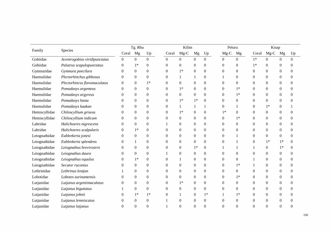
100

Family Species Tg. Rhu Kilim Peluru Kisap

Coral Mg Up Coral Mg-C Mg Up Mg-C Mg Coral Mg-C Mg Up

Gobiidae Acentrogobius viridipunctatus 0 0 0 0 0 0 0 0 0 1* 0 0 0

Gobiidae Palutrus scapulopunctatus 0 1* 0 0 0 0 0 0 0 1* 0 0 0

Gymnuridae Gymnura poecilura 0 0 0 0 1* 0 0 0 0 0 0 0 0

Haemulidae Plectorhinchus gibbosus 0 0 0 0 1 1 0 1 0 0 0 0 0

Haemulidae Plectorhincus flavomaculatus 0 0 1* 0 0 0 0 0 0 0 0 0 0

Haemulidae Pomadasys argenteus 0 0 0 0 1* 0 0 0 1* 0 0 0 0

Haemulidae Pomadasys argyreus 0 0 0 0 0 0 0 0 1* 0 0 0 0

Haemulidae Pomadasys hasta 0 0 0 0 1* 1* 0 0 0 0 0 0 0

Haemulidae Pomadasys kaakan 0 0 0 0 1 1 1 0 1 0 1* 0 1

Hemiscyllidae Chiloscyllium griseus 0 0 0 0 1* 0 0 1* 0 0 0 0 0

Hemiscyllidae Chiloscyllium indicum 0 0 0 0 0 0 0 0 1* 0 0 0 0

Labridae Halichoeres nigrescens 0 0 0 1 0 0 0 0 0 0 0 0 0

Labridae Halichoeres scalpularis 0 1* 0 0 0 0 0 0 0 0 0 0 0

Leiognathidae Eubleekeria jonesi 0 0 0 0 0 0 0 0 1 0 0 0 0

Leiognathidae Eubleekeria splendens 0 1 0 0 0 0 0 0 1 0 1* 1* 0

Leiognathidae Leiognathus brevirostris 0 0 0 0 0 1* 0 1 1 1 0 1* 0

Leiognathidae Leiognathus daura 0 0 0 1 0 0 0 0 0 0 0 0 0

Leiognathidae Leiognathus equulus 0 1* 0 0 1 0 0 0 0 1 0 0 0

Leiognathidae Secutor ruconius 0 0 0 0 0 0 0 0 1* 1 0 0 0

Lethrinidae Lethrinus lentjan 1 0 0 0 0 0 0 0 0 0 0 0 0

Lobotidae Lobotes surinamensis 0 0 0 0 0 0 0 0 1* 0 0 0 0

Lutjanidae Lutjanus argentimaculatus 0 0 0 0 1* 0 0 0 0 0 0 0 0

Lutjanidae Lutjanus biguttatus 1 0 0 0 0 0 0 0 0 0 0 0 0

Lutjanidae Lutjanus johnii 0 1* 1* 0 1 0 1* 1 1* 0 0 0 0

Lutjanidae Lutjanus lemniscatus 0 0 0 1 0 0 0 0 0 0 0 0 0

Lutjanidae Lutjanus lutjanus 0 0 0 1 0 0 0 0 0 0 0 0 0

101

Family Species Tg. Rhu Kilim Peluru Kisap

Coral Mg Up Coral Mg-C Mg Up Mg-C Mg Coral Mg-C Mg Up

Lutjanidae Lutjanus russelli 1 0 1 0 1 1 0 1 0 0 0 0 0

Lutjanidae Lutjanus stellatus 0 0 0 0 1* 0 0 0 0 0 0 0 0

Lutjanidae Lutjanus vitta 1 0 0 1 0 0 0 0 0 0 0 0 0

Megalopidae Megalops cyprinoides 0 0 0 0 1* 0 0 0 0 0 0 0 0

Monacanthidae Acreichthys tomentosus 0 1* 0 0 0 0 0 0 0 0 0 0 0

Monacanthidae Monacanthus choirocephalus 0 1* 0 0 0 0 0 0 0 0 0 0 0

Monachantidae Monachanthus chinensis 1 0 0 0 1 0 1* 1* 0 1 0 0 0

Mugilidae Chelon macrolepis 0 0 0 0 0 0 0 0 1* 0 0 1* 0

Mugilidae Chelon subviridis 0 0 0 1 0 1 1 0 1 0 1* 1 1

Mugilidae Ellochelon vaigiensis 1 1* 0 1 0 0 0 0 1* 1 0 0 1

Mugilidae Liza tade 0 0 0 0 0 0 0 0 1* 0 0 1* 0

Mugilidae Moolgarda perusii 1 1 0 1 0 0 0 0 0 0 0 1 0

Mugilidae Moolgarda seheli 0 0 1 1 0 1 1 0 1 1 0 1 1

Mugilidae Paramugil parmatus 0 0 0 1 0 0 0 0 0 0 0 0 0

Mugilidae Valamugil buchanani 0 1* 1 1 1 0 0 0 0 0 0 0 0

Mugillidae Valamugil cunnesius 0 0 0 0 0 0 0 0 1* 1* 1* 1* 0

Mullidae Upeneus bensasi 0 1* 0 0 0 0 0 0 0 0 0 0 0

Mullidae Upeneus sulphureus 0 1 0 0 0 0 0 0 0 0 0 0 0

Mullidae Upeneus sundaicus 0 0 0 1 0 0 0 0 0 0 0 0 0

Mullidae Upeneus tragula 0 0 0 1 0 0 0 0 0 0 0 0 0

Myliobatidae Aetomylaeus maculatus 0 0 0 0 0 0 0 1* 0 0 1* 0 0

Nemipteridae Nemipterus hexodon 0 0 0 0 0 0 0 0 0 1 0 0 0

Nemipteridae Scolopsis ciliata 1 0 0 0 0 0 0 0 0 0 0 0 0

Nemipteridae Scolopsis vosmeri 0 0 0 1 1 0 0 0 0 0 0 0 0

Ostraciidae Ostracion rhinorhynchos 0 0 0 0 0 0 1* 0 0 0 0 0 0

Ostraciidae Ostracion cubicus 0 0 0 0 0 0 1 0 0 0 0 0 0

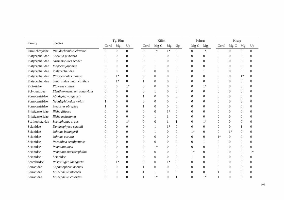
102

Family Species Tg. Rhu Kilim Peluru Kisap

Coral Mg Up Coral Mg-C Mg Up Mg-C Mg Coral Mg-C Mg Up

Paralichthyidae Pseudorhombus elevatus 0 0 0 0 1* 1* 0 0 1* 0 0 0 0

Platycephalidae Cociella punctata 0 0 0 0 1 0 0 0 0 0 0 0 0

Platycephalidae Grammoplites scaber 0 0 0 0 1 0 0 0 0 0 0 0 0

Platycephalidae Inegocia japonica 0 0 0 0 1 0 0 0 0 0 0 0 0

Platycephalidae Platycephalidae 0 0 0 0 0 0 0 0 1 0 0 0 0

Platycephalidae Platycephalus indicus 0 1* 0 0 0 0 0 0 0 0 0 1* 0

Platycephalidae Suggrundus macracanthus 0 1* 0 1 0 0 0 0 0 0 0 0 0

Plotosidae Plotosus canius 0 0 1* 0 0 0 0 0 1* 0 0 0 0

Polynemidae Eleutheronema tetradactylum 0 0 0 0 1 0 0 0 0 0 0 0 0

Pomacentridae Abudefdef vaigiensis 0 0 0 1 0 0 0 0 0 0 0 0 0

Pomacentridae Neoglyphidodon melas 1 0 0 0 0 0 0 0 0 0 0 0 0

Pomacentridae Stegastes obreptus 1 0 0 1 0 0 0 0 0 0 0 0 0

Pristigasteridae Ilisha filigera 0 0 0 0 0 1* 0 0 0 0 0 0 0

Pristigasteridae Ilisha melastoma 0 0 0 0 1 1 0 0 0 0 0 0 0

Scathophagidae Scatophagus argus 0 0 1* 0 0 1 1 0 1* 0 0 0 0

Scianidae Dendrophyssa russelli 0 0 0 0 1 1* 0 0 0 0 0 1 0

Scianidae Johnius belangerii 0 0 0 0 1 0 0 1* 0 0 1* 0 0

Scianidae Johnius carutta 0 0 0 0 0 0 0 0 0 1* 0 0 0

Scianidae Paranibea semiluctuosa 0 0 0 0 0 0 0 0 1 0 0 0 0

Scianidae Pennahia anea 0 0 0 0 1* 0 0 0 0 0 0 0 0

Scianidae Pennahia macrocephalus 0 0 0 0 0 0 0 1* 0 0 0 0 1*

Scianidae Scianidae 0 0 0 0 0 0 0 1 0 0 0 0 0

Scombridae Rastrelliger kanagurta 0 1* 0 0 0 1* 0 0 0 0 0 0 0

Serranidae Cephalopholis boenak 0 0 0 1 0 0 0 0 0 0 0 0 0

Serranidae Epinephelus bleekeri 0 0 0 1 1 0 0 0 0 1 0 0 0

Serranidae Epinephelus coioides 0 0 0 1 1* 0 1 0 1* 1 0 0 0

103

Family Species Tg. Rhu Kilim Peluru Kisap

Coral Mg Up Coral Mg-C Mg Up Mg-C Mg Coral Mg-C Mg Up

Serranidae Epinephelus erythrurus 0 0 0 1 0 0 0 0 0 0 0 0 0

Serranidae Epinephelus malabaricus 0 0 0 0 1 0 0 0 0 0 0 0 0

Serranidae Epinephelus quoyanus 1 0 0 0 0 0 0 0 0 0 0 0 0

Serranidae Epinephelus sexfasciatus 0 0 0 1 0 0 0 0 1* 0 0 0 0

Siganidae Siganus fuscescens 0 0 0 0 0 0 0 0 0 1 0 0 0

Siganidae Siganus javus 0 1* 0 1 1 0 1 0 0 1 0 0 0

Sillaginidae Sillago aeolus 0 0 0 1 0 0 0 0 0 1 0 0 0

Sillaginidae Sillago sihama 0 1 0 1 1 1* 1 1 1 0 0 0 1

Sparidae Acanthopagrus berda 0 1* 0 0 0 0 0 0 0 0 0 0 0

Sparidae Dentex angolensis 0 1* 0 0 0 0 0 0 0 0 0 0 0

Sphyraenidae Sphyraena barracuda 0 1* 0 0 0 0 0 0 0 0 0 1 0

Sphyraenidae Sphyraena jello 0 0 0 0 1 1 0 0 1 1 0 0 0

Sphyraenidae Sphyraena sp. 0 0 0 0 0 1 0 0 0 0 0 0 0

Synodontidae Saurida tumbil 0 0 0 0 0 0 0 0 1* 0 0 0 0

Tetraodontidae Chelonodon patoca 0 1* 0 0 0 0 0 0 0 0 0 0 0

Tetraodontidae Lagocephalus lunaris 0 0 0 0 0 1 0 0 0 0 0 0 0

Tetraodontidae Tetraodon fluviatilis 0 1* 0 0 0 0 0 0 0 0 0 1* 0

Tetraodontidae Tetraodon nigroviridis 0 0 0 0 0 0 1 0 0 0 0 1 0

Toxotidae Toxotes jaculatrix 0 0 1 0 0 0 0 0 1* 0 0 1* 1

Triacanthidae Pseudotriacanthus strigilifer 1 0 0 0 0 0 0 0 1 0 0 0 0

Triacanthidae Triacanthus biaculeatus 1 0 0 0 0 1 0 0 1 0 1* 1* 1

TOTAL 18 36 10 35 47 37 19 16 40 22 29 10 19

104

APPENDIX II

Details of PCA on dietary composition of fish species computed in Canoco software.

No samples omitted

Number of samples 63

Number of species 14

Number of occurrences 260

No transformation of species data

No species-weights specified

No sample-weights specified

Centering/standardization by species = 1

Centering/standardization by samples = 0

No. of active samples: 63

No. of passive samples: 0

No. of active species: 14

Total sum of squares in species data = 148901.

Total standard deviation in species data TAU = 12.9932

**** Summary ****

Axes 1 2 3 4 Total

variance

Eigenvalues : 0.289 0.189 0.125 0.09 1

Cumulative

percentage variance

of species data :

28.9 47.8 60.3 69.3

Sum of all eigenvalues 1.000

105

APPENDIX III

Results of the non-parametric Kruskal-Wallis analysis on stable isotope signatures.

a) Results of the non-parametric Kruskal-Wallis analysis of δ13

C between feeding

guilds, Kruskal-Wallis chi-squared, χ2 = 51.6659, df = 4, p-value = 1.62

e-10

Pairwise comparisons using Wilcoxon rank sum test

Carnivore Herbivore Invertivore Omnivore

Herbivore 3.70E-09

* - - -

Invertivore 2.80E-03

* 3.10E-06

* - -

Omnivore 0.0081* 0.1468 0.4398 -

Piscivore 0.4019 1.20E-03

* 0.4398 0.4398 *denotes pairs of significant different

b) Results of the non-parametric Kruskal-Wallis analysis of δ15

N between feeding

guilds, Kruskal-Wallis chi-squared, χ2 = 173.7278, df = 4, p-value < 2.2

e-16

Pairwise comparisons using Wilcoxon rank sum test

Carnivore Herbivore Invertivore Omnivore

Herbivore < 2e-16

* - - -

Invertivore 0.47 < 2e-16

* - -

Omnivore 0.00* 0.00* 0.00* -

Piscivore 0.00* 0.00* 0.00* 0.00* *denotes pairs of significant different

c) Result of the non-parametric Kruskal-Wallis analysis of δ13

C between habitat

zones, Kruskal-Wallis chi-squared, χ2 = 33.7551, df = 3, p-value = 2.232

e-07

Pairwise comparisons using Wilcoxon rank sum test

Coral Mangrove Mg-C

Mangrove 0.00028* - -

Mg-C 0.00555* 0.29527 -

Up 3.20E-06

* 0.00555* 0.00078* *denotes pairs of significant different

d) Results of the non-parametric Kruskal-Wallis analysis of δ15

N between habitat

zones, Kruskal-Wallis chi-squared, χ2 = 53.6565, df = 3, p-value = 1.328

e-11

Pairwise comparisons using Wilcoxon rank sum test

Coral Mangrove Mg-C

Mangrove 5.90E-06

* - -

Mg-C 0.41 4.10E-08

* -

Up 5.10E-05

* 0.28 5.30E-06

* *denotes pairs of significant different

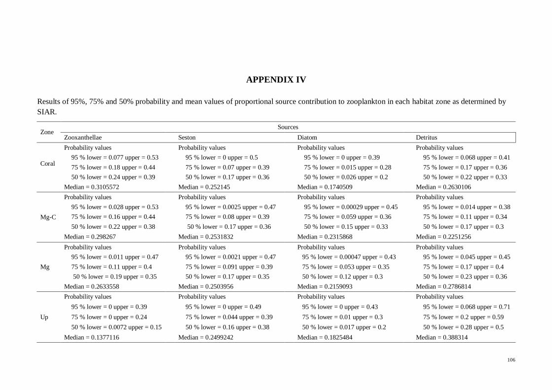
106

APPENDIX IV

Results of 95%, 75% and 50% probability and mean values of proportional source contribution to zooplankton in each habitat zone as determined by

SIAR.

Zone Sources

Zooxanthellae Seston Diatom Detritus

Coral

Probability values Probability values Probability values Probability values

95 % lower = 0.077 upper = 0.53 95 % lower = 0 upper = 0.5 95 % lower = 0 upper = 0.39 95 % lower = 0.068 upper = 0.41

75 % lower = 0.18 upper = 0.44 75 % lower = 0.07 upper = 0.39 75 % lower = 0.015 upper = 0.28 75 % lower = 0.17 upper = 0.36

50 % lower = 0.24 upper = 0.39 50 % lower = 0.17 upper = 0.36 50 % lower = 0.026 upper = 0.2 50 % lower = 0.22 upper = 0.33

Median = 0.3105572 Median = 0.252145 Median = 0.1740509 Median = 0.2630106

Mg-C

Probability values Probability values Probability values Probability values

95 % lower = 0.028 upper = 0.53 95 % lower = 0.0025 upper = 0.47 95 % lower = 0.00029 upper = 0.45 95 % lower = 0.014 upper = 0.38

75 % lower = 0.16 upper = 0.44 75 % lower = 0.08 upper = 0.39 75 % lower = 0.059 upper = 0.36 75 % lower = 0.11 upper = 0.34

50 % lower = 0.22 upper = 0.38 50 % lower = 0.17 upper = 0.36 50 % lower = 0.15 upper = 0.33 50 % lower = 0.17 upper = 0.3

Median = 0.298267 Median = 0.2531832 Median = 0.2315868 Median = 0.2251256

Mg

Probability values Probability values Probability values Probability values

95 % lower = 0.011 upper = 0.47 95 % lower = 0.0021 upper = 0.47 95 % lower = 0.00047 upper = 0.43 95 % lower = 0.045 upper = 0.45

75 % lower = 0.11 upper = 0.4 75 % lower = 0.091 upper = 0.39 75 % lower = 0.053 upper = 0.35 75 % lower = 0.17 upper = 0.4

50 % lower = 0.19 upper = 0.35 50 % lower = 0.17 upper = 0.35 50 % lower = 0.12 upper = 0.3 50 % lower = 0.23 upper = 0.36

Median = 0.2633558 Median = 0.2503956 Median = 0.2159093 Median = 0.2786814

Up

Probability values Probability values Probability values Probability values

95 % lower = 0 upper = 0.39 95 % lower = 0 upper = 0.49 95 % lower = 0 upper = 0.43 95 % lower = 0.068 upper = 0.71

75 % lower = 0 upper = 0.24 75 % lower = 0.044 upper = 0.39 75 % lower = 0.01 upper = 0.3 75 % lower = 0.2 upper = 0.59

50 % lower = 0.0072 upper = 0.15 50 % lower = 0.16 upper = 0.38 50 % lower = 0.017 upper = 0.2 50 % lower = 0.28 upper = 0.5

Median = 0.1377116 Median = 0.2499242 Median = 0.1825484 Median = 0.388314

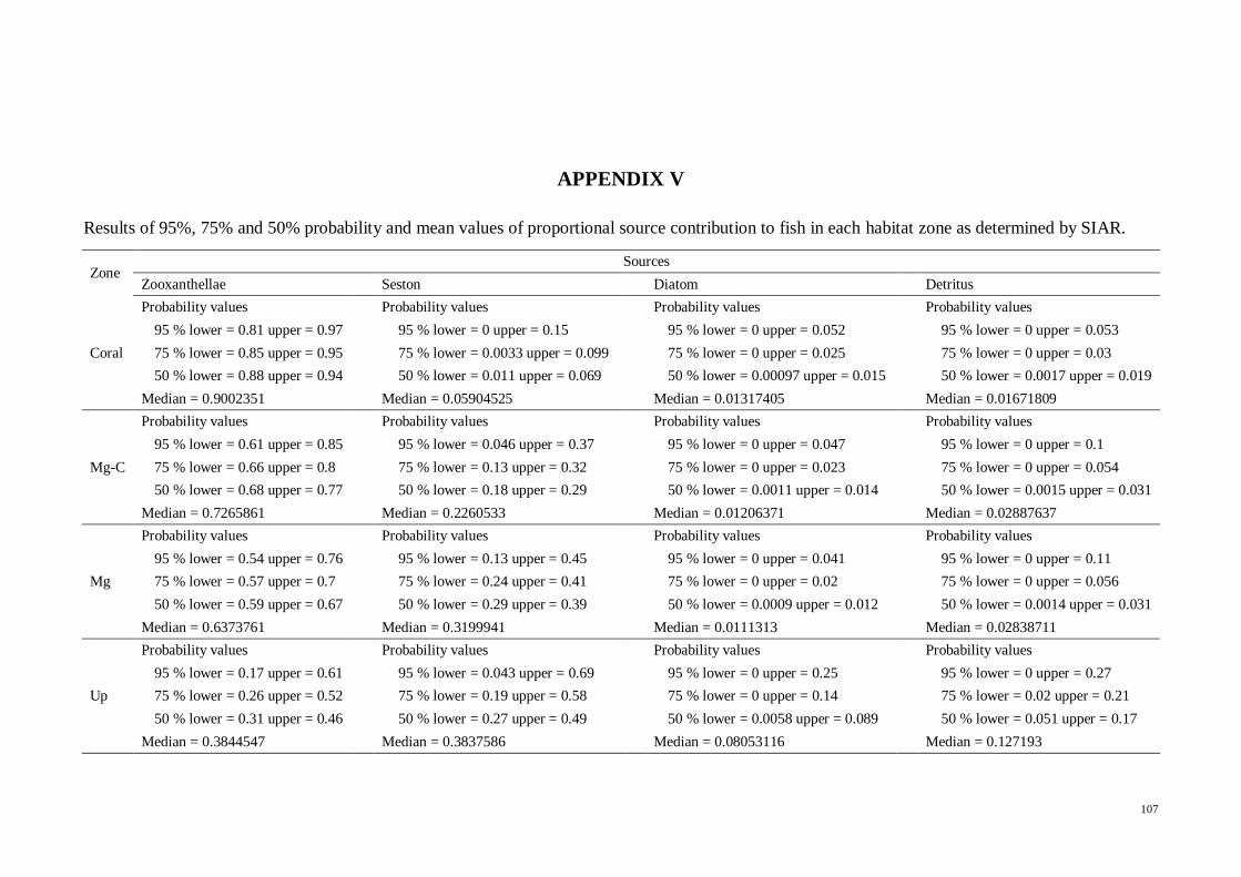
107

APPENDIX V

Results of 95%, 75% and 50% probability and mean values of proportional source contribution to fish in each habitat zone as determined by SIAR.

Zone Sources

Zooxanthellae Seston Diatom Detritus

Coral

Probability values Probability values Probability values Probability values

95 % lower = 0.81 upper = 0.97 95 % lower = 0 upper = 0.15 95 % lower = 0 upper = 0.052 95 % lower = 0 upper = 0.053

75 % lower = 0.85 upper = 0.95 75 % lower = 0.0033 upper = 0.099 75 % lower = 0 upper = 0.025 75 % lower = 0 upper = 0.03

50 % lower = 0.88 upper = 0.94 50 % lower = 0.011 upper = 0.069 50 % lower = 0.00097 upper = 0.015 50 % lower = 0.0017 upper = 0.019

Median = 0.9002351 Median = 0.05904525 Median = 0.01317405 Median = 0.01671809

Mg-C

Probability values Probability values Probability values Probability values

95 % lower = 0.61 upper = 0.85 95 % lower = 0.046 upper = 0.37 95 % lower = 0 upper = 0.047 95 % lower = 0 upper = 0.1

75 % lower = 0.66 upper = 0.8 75 % lower = 0.13 upper = 0.32 75 % lower = 0 upper = 0.023 75 % lower = 0 upper = 0.054

50 % lower = 0.68 upper = 0.77 50 % lower = 0.18 upper = 0.29 50 % lower = 0.0011 upper = 0.014 50 % lower = 0.0015 upper = 0.031

Median = 0.7265861 Median = 0.2260533 Median = 0.01206371 Median = 0.02887637

Mg

Probability values Probability values Probability values Probability values

95 % lower = 0.54 upper = 0.76 95 % lower = 0.13 upper = 0.45 95 % lower = 0 upper = 0.041 95 % lower = 0 upper = 0.11

75 % lower = 0.57 upper = 0.7 75 % lower = 0.24 upper = 0.41 75 % lower = 0 upper = 0.02 75 % lower = 0 upper = 0.056

50 % lower = 0.59 upper = 0.67 50 % lower = 0.29 upper = 0.39 50 % lower = 0.0009 upper = 0.012 50 % lower = 0.0014 upper = 0.031

Median = 0.6373761 Median = 0.3199941 Median = 0.0111313 Median = 0.02838711

Up

Probability values Probability values Probability values Probability values

95 % lower = 0.17 upper = 0.61 95 % lower = 0.043 upper = 0.69 95 % lower = 0 upper = 0.25 95 % lower = 0 upper = 0.27

75 % lower = 0.26 upper = 0.52 75 % lower = 0.19 upper = 0.58 75 % lower = 0 upper = 0.14 75 % lower = 0.02 upper = 0.21

50 % lower = 0.31 upper = 0.46 50 % lower = 0.27 upper = 0.49 50 % lower = 0.0058 upper = 0.089 50 % lower = 0.051 upper = 0.17

Median = 0.3844547 Median = 0.3837586 Median = 0.08053116 Median = 0.127193

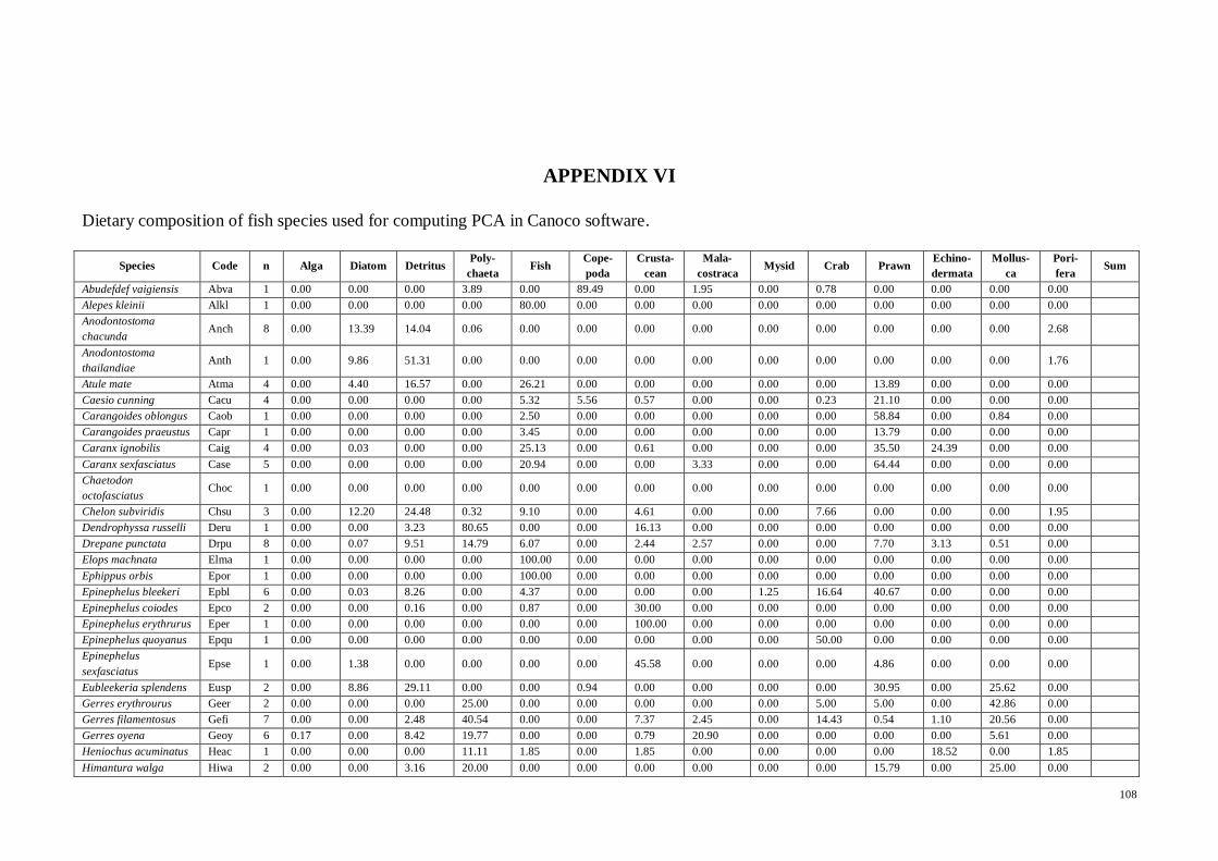
108

APPENDIX VI

Dietary composition of fish species used for computing PCA in Canoco software.

Species Code n Alga Diatom Detritus Poly-

chaeta Fish

Cope-

poda

Crusta-

cean

Mala-

costraca Mysid Crab Prawn

Echino-

dermata

Mollus-

ca

Pori-

fera Sum

Abudefdef vaigiensis Abva 1 0.00 0.00 0.00 3.89 0.00 89.49 0.00 1.95 0.00 0.78 0.00 0.00 0.00 0.00

Alepes kleinii Alkl 1 0.00 0.00 0.00 0.00 80.00 0.00 0.00 0.00 0.00 0.00 0.00 0.00 0.00 0.00

Anodontostoma

chacunda Anch 8 0.00 13.39 14.04 0.06 0.00 0.00 0.00 0.00 0.00 0.00 0.00 0.00 0.00 2.68

Anodontostoma

thailandiae Anth 1 0.00 9.86 51.31 0.00 0.00 0.00 0.00 0.00 0.00 0.00 0.00 0.00 0.00 1.76

Atule mate Atma 4 0.00 4.40 16.57 0.00 26.21 0.00 0.00 0.00 0.00 0.00 13.89 0.00 0.00 0.00

Caesio cunning Cacu 4 0.00 0.00 0.00 0.00 5.32 5.56 0.57 0.00 0.00 0.23 21.10 0.00 0.00 0.00

Carangoides oblongus Caob 1 0.00 0.00 0.00 0.00 2.50 0.00 0.00 0.00 0.00 0.00 58.84 0.00 0.84 0.00

Carangoides praeustus Capr 1 0.00 0.00 0.00 0.00 3.45 0.00 0.00 0.00 0.00 0.00 13.79 0.00 0.00 0.00

Caranx ignobilis Caig 4 0.00 0.03 0.00 0.00 25.13 0.00 0.61 0.00 0.00 0.00 35.50 24.39 0.00 0.00

Caranx sexfasciatus Case 5 0.00 0.00 0.00 0.00 20.94 0.00 0.00 3.33 0.00 0.00 64.44 0.00 0.00 0.00

Chaetodon

octofasciatus Choc 1 0.00 0.00 0.00 0.00 0.00 0.00 0.00 0.00 0.00 0.00 0.00 0.00 0.00 0.00

Chelon subviridis Chsu 3 0.00 12.20 24.48 0.32 9.10 0.00 4.61 0.00 0.00 7.66 0.00 0.00 0.00 1.95

Dendrophyssa russelli Deru 1 0.00 0.00 3.23 80.65 0.00 0.00 16.13 0.00 0.00 0.00 0.00 0.00 0.00 0.00

Drepane punctata Drpu 8 0.00 0.07 9.51 14.79 6.07 0.00 2.44 2.57 0.00 0.00 7.70 3.13 0.51 0.00

Elops machnata Elma 1 0.00 0.00 0.00 0.00 100.00 0.00 0.00 0.00 0.00 0.00 0.00 0.00 0.00 0.00

Ephippus orbis Epor 1 0.00 0.00 0.00 0.00 100.00 0.00 0.00 0.00 0.00 0.00 0.00 0.00 0.00 0.00

Epinephelus bleekeri Epbl 6 0.00 0.03 8.26 0.00 4.37 0.00 0.00 0.00 1.25 16.64 40.67 0.00 0.00 0.00

Epinephelus coiodes Epco 2 0.00 0.00 0.16 0.00 0.87 0.00 30.00 0.00 0.00 0.00 0.00 0.00 0.00 0.00

Epinephelus erythrurus Eper 1 0.00 0.00 0.00 0.00 0.00 0.00 100.00 0.00 0.00 0.00 0.00 0.00 0.00 0.00

Epinephelus quoyanus Epqu 1 0.00 0.00 0.00 0.00 0.00 0.00 0.00 0.00 0.00 50.00 0.00 0.00 0.00 0.00

Epinephelus

sexfasciatus Epse 1 0.00 1.38 0.00 0.00 0.00 0.00 45.58 0.00 0.00 0.00 4.86 0.00 0.00 0.00

Eubleekeria splendens Eusp 2 0.00 8.86 29.11 0.00 0.00 0.94 0.00 0.00 0.00 0.00 30.95 0.00 25.62 0.00

Gerres erythrourus Geer 2 0.00 0.00 0.00 25.00 0.00 0.00 0.00 0.00 0.00 5.00 5.00 0.00 42.86 0.00

Gerres filamentosus Gefi 7 0.00 0.00 2.48 40.54 0.00 0.00 7.37 2.45 0.00 14.43 0.54 1.10 20.56 0.00

Gerres oyena Geoy 6 0.17 0.00 8.42 19.77 0.00 0.00 0.79 20.90 0.00 0.00 0.00 0.00 5.61 0.00

Heniochus acuminatus Heac 1 0.00 0.00 0.00 11.11 1.85 0.00 1.85 0.00 0.00 0.00 0.00 18.52 0.00 1.85

Himantura walga Hiwa 2 0.00 0.00 3.16 20.00 0.00 0.00 0.00 0.00 0.00 0.00 15.79 0.00 25.00 0.00

109

Inegocia japonica Inja 2 0.00 0.00 0.00 0.00 50.00 0.00 0.00 0.00 0.00 0.00 31.25 0.00 0.00 0.00

Lagocephalus lunaris Lalu 5 0.00 0.00 0.00 0.00 0.00 0.00 0.00 0.00 0.00 99.00 0.00 0.00 1.00 0.00

Leiognathus

brevirostris Lebr 3 0.00 8.73 16.65 0.00 0.00 4.75 0.00 0.19 0.00 0.00 13.17 0.00 1.90 0.33

Leiognathus equulus Leeq 1 0.00 0.00 35.71 0.00 0.00 0.00 0.00 0.00 0.00 0.00 21.43 0.00 0.00 0.00

Leiognathus splendens Lesp 3 0.00 0.00 13.18 26.65 0.00 1.72 0.00 0.00 0.00 0.00 0.00 0.00 0.00 0.00

Leoignathus daura Leda 3 0.00 0.00 2.79 0.67 1.00 0.14 0.14 1.05 0.00 4.73 1.39 0.81 3.76 0.00

Lethrinus lentjan Lele 2 0.00 0.00 0.00 0.00 0.00 0.00 25.00 0.00 0.00 50.00 0.00 0.00 0.00 0.00

Lutjanus johnii Lujo 4 0.00 0.00 0.35 0.00 43.75 0.00 1.41 2.08 2.82 17.31 26.16 0.00 4.01 0.00

Lutjanus lemniscatus Lule 3 0.00 0.00 0.00 0.00 96.00 0.00 0.00 0.00 0.00 0.00 4.00 0.00 0.00 0.00

Lutjanus lutjanus Lulu 2 0.00 0.00 0.00 0.00 11.01 7.58 0.43 7.58 0.00 7.58 43.10 0.00 0.00 0.00

Lutjanus russelli Luru 4 0.00 0.00 0.00 0.00 0.00 0.00 0.00 0.00 0.00 0.00 100.00 0.00 0.00 0.00

Lutjanus vitta Luvi 4 0.00 0.00 0.00 0.00 39.41 0.00 0.20 0.00 0.00 0.00 34.48 0.00 0.00 0.00

Monachanthus

chinensis Moch 4 0.00 0.03 30.71 0.35 0.00 0.00 8.01 0.12 0.00 4.00 0.00 10.16 1.27 0.03

Moolgarda seheli Mose 4 0.00 7.53 17.52 0.00 0.00 0.00 0.12 0.00 0.00 0.00 0.00 0.00 0.00 0.52

Paranibea

semiluctuosa Pase 1 0.00 0.00 0.00 0.00 0.00 4.35 0.00 0.00 8.70 0.00 86.96 0.00 0.00 0.00

Platycephalidae Plat 4 0.00 0.00 0.00 0.00 0.00 0.00 0.00 0.00 0.00 33.33 66.67 0.00 0.00 0.00

Plectorhincus gibossus Plgi 10 0.00 0.14 0.38 3.62 11.38 0.77 1.69 0.00 0.00 38.98 20.61 0.00 1.17 0.05

Pomadasys kaakan Poka 10 0.00 0.04 2.36 4.00 8.11 0.11 3.40 0.11 0.00 17.08 21.86 0.00 0.00 0.01

Pseudotriacanthus

strigilifer Psst 2 0.00 0.00 7.89 0.00 0.00 0.00 0.56 8.95 0.00 22.37 2.45 41.65 4.70 0.00

Scolopsis ciliata Scci 5 0.00 0.00 24.10 26.10 0.00 0.00 0.80 2.01 0.00 6.02 0.80 4.02 0.00 0.00

Scolopsis vosmeri Scvo 3 0.00 0.00 4.12 0.73 0.00 0.00 0.00 0.13 0.00 48.33 0.36 3.30 0.73 0.00

Scomberoides

commersonnianus Scco 8 0.00 0.00 0.13 0.00 48.84 0.00 0.00 0.00 0.00 0.00 25.00 0.00 0.00 0.00

Scomberoides lysan Scly 3 0.00 0.00 0.00 0.00 67.21 0.00 0.00 0.00 0.00 0.00 0.00 0.00 0.00 0.00

Scomberoides tol Scto 2 0.00 0.00 0.00 0.00 24.00 0.00 0.00 0.00 0.00 0.00 0.00 0.00 0.00 0.00

Siganus fuscescens Sifu 4 79.68 0.00 0.00 0.00 0.00 0.40 0.00 0.00 0.00 0.00 0.00 0.00 0.00 0.00

Siganus javus Sija 5 6.74 1.61 13.44 0.05 0.00 0.97 0.00 0.11 0.00 0.00 0.00 0.21 0.30 44.08

Sillago aeolus Siae 4 0.00 0.00 0.00 0.00 0.00 0.00 0.00 0.00 0.00 35.29 0.00 0.00 0.00 0.00

Sillago sihama Sisi 5 0.00 0.00 1.39 1.39 0.00 0.00 10.63 10.91 0.00 20.00 26.11 0.00 0.00 0.00

Sphyraena jello Spje 3 0.00 0.55 6.36 0.00 62.22 0.00 0.00 0.00 0.00 0.00 0.00 0.00 4.44 0.00

Thryssa hamiltonii Thha 5 0.00 0.00 0.00 0.00 0.00 0.00 0.00 0.00 100.00 0.00 0.00 0.00 0.00 0.00

Toxotes jaculatrix Toja 2 0.00 0.00 0.00 0.00 0.00 0.00 0.00 0.00 0.00 26.98 25.40 0.00 0.00 0.00

Triacanthus

biaculeatus Trbi 2 0.00 0.00 6.00 1.50 0.00 0.00 0.00 0.00 0.00 8.51 0.00 0.00 47.46 0.00

110

Tylosurus crocodilus

crocodilus Tycc 2 0.00 0.00 0.00 0.00 100.00 0.00 0.00 0.00 0.00 0.00 0.00 0.00 0.00 0.00

Upeneus sundaicus Upsu 5 0.00 0.00 0.00 0.00 0.00 0.00 0.00 0.00 0.00 50.00 5.56 11.11 33.33 0.00

Upeneus tragula Uptr 5 0.00 0.00 0.00 0.00 0.00 0.00 25.93 0.00 0.00 0.00 74.07 0.00 0.00 0.00

Valamugil buchanani Vabu 5 0.00 26.01 11.32 0.00 0.00 0.00 0.00 0.00 0.00 0.00 0.00 0.00 0.00 1.91

Sum 86.592 94.860 365.119 281.199 948.730 116.771 288.274 64.431 112.763 584.266 943.894 118.393 225.078 55.170 4285.539

Mean 1.374 1.506 5.796 4.463 15.059 1.854 4.576 1.023 1.790 9.274 14.982 1.879 3.573 0.876

VOL% 2.021 2.213 8.520 6.562 22.138 2.725 6.727 1.503 2.631 13.633 22.025 2.763 5.252 1.287 100.000

FO 3 17 30 20 27 12 24 16 4 24 34 11 19 12 253

FO% 1.186 6.719 11.858 7.905 10.672 4.743 9.486 6.324 1.581 9.486 13.439 4.348 7.510 4.743

111

APPENDIX VII

Fish stable isotope signatures for carbon, δ13

C and nitrogen, δ15

N with trophic

fractionation correction for carbon, ∆13

C and nitrogen, ∆15

N used in computing SIAR.

Habitat Species Feeding

guilds δ

13C ∆

13C δ

15N ∆

15N C:N

Coral Chelon subviridis Herbivore -12.01 -12.96 9.34 6.65 3.76

Coral Moolgarda perusii Herbivore -10.44 -11.39 10.90 8.21 4.08

Coral Moolgarda perusii Herbivore -10.49 -11.44 7.23 4.54 3.78

Coral Moolgarda perusii Herbivore -10.59 -11.54 7.29 4.60 3.86

Coral Moolgarda perusii Herbivore -14.18 -15.13 9.16 6.47 3.96

Coral Moolgarda seheli Herbivore -12.69 -13.64 7.17 4.48 3.85

Coral Moolgarda seheli Herbivore -9.97 -10.92 8.07 5.38 3.79

Coral Paramugil parmatus Herbivore -8.88 -9.83 7.47 4.78 3.82

Coral Valamugil buchanani Herbivore -9.67 -10.62 8.06 5.37 3.80

Coral Valamugil buchanani Herbivore -10.40 -11.35 8.99 6.30 3.78

Coral Chaetodon octofasciatus Omnivore -13.52 -14.92 11.94 7.76 3.76

Coral Chaetodon octofasciatus Omnivore -13.36 -14.76 11.70 7.52 3.84

Coral Ellochelon vaigiensis Omnivore -11.40 -12.80 9.88 5.71 3.68

Coral Ellochelon vaigiensis Omnivore -11.01 -12.41 9.69 5.52 3.71

Coral Ellochelon vaigiensis Omnivore -11.24 -12.64 9.16 4.98 3.77

Coral Gerres oyena Omnivore -12.07 -13.47 12.05 7.87 3.76

Coral Gerres oyena Omnivore -14.34 -15.74 12.54 8.37 3.72

Coral Gerres oyena Omnivore -14.64 -16.04 11.74 7.56 3.73

Coral Gerres oyena Omnivore -13.61 -15.01 11.68 7.50 3.83

Coral Siganus javus Omnivore -16.62 -18.02 12.70 8.52 3.82

Coral Siganus javus Omnivore -21.10 -22.50 10.99 6.82 3.73

Coral Abudefduf vaigiensis Invertivore -18.27 -19.67 11.69 7.34 3.75

Coral Drepane punctata Invertivore -15.72 -17.12 13.45 9.10 3.77

Coral Drepane punctata Invertivore -15.79 -17.19 13.19 8.84 3.81

Coral Epinephelus coioides Invertivore -13.68 -15.08 11.82 7.47 3.77

Coral Epinephelus coioides Invertivore -15.87 -17.27 14.08 9.73 3.75

Coral Epinephelus erythrurus Invertivore -13.17 -14.57 12.15 7.80 3.78

Coral Epinephelus sexfasciatus Invertivore -15.83 -17.23 13.64 9.29 3.78

Coral Epinephelus sexfasciatus Invertivore -16.12 -17.52 12.96 8.61 3.82

Coral Himantura walga Invertivore -14.67 -16.07 12.16 7.81 3.38

Coral Leiognathus daura Invertivore -16.77 -18.17 13.09 8.74 3.81

Coral Leiognathus daura Invertivore -16.54 -17.94 13.04 8.69 3.73

Coral Leiognathus daura Invertivore -16.31 -17.71 13.78 9.43 3.80

Coral Lutjanus russelli Invertivore -12.93 -14.33 11.70 7.35 3.69

Coral Lutjanus russelli Invertivore -16.02 -17.42 11.66 7.31 3.72

Coral Lutjanus russelli Invertivore -15.30 -16.70 12.44 8.09 3.72

Coral Scolopsis vosmeri Invertivore -16.44 -17.84 13.69 9.34 4.23

Coral Scolopsis vosmeri Invertivore -16.47 -17.87 12.97 8.62 3.83

Coral Sillago aeolus Invertivore -13.87 -15.27 12.30 7.95 3.77

Coral Sillago sihama Invertivore -13.68 -15.08 12.86 8.51 3.72

Coral Upeneus sundaicus Invertivore -14.98 -16.38 13.27 8.92 3.73

112

Habitat Species Feeding

guilds δ

13C ∆

13C δ

15N ∆

15N C:N

Coral Upeneus sundaicus Invertivore -15.83 -17.23 13.87 9.52 3.81

Coral Atule mate Carnivore -15.87 -17.63 12.96 7.48 3.74

Coral Atule mate Carnivore -15.81 -17.57 13.09 7.61 3.81

Coral Atule mate Carnivore -15.86 -17.62 12.69 7.21 3.70

Coral Caesio cunning Carnivore -16.31 -18.07 12.60 7.11 3.82

Coral Caesio cunning Carnivore -16.57 -18.33 12.92 7.44 3.72

Coral Caesio cunning Carnivore -17.08 -18.84 12.59 7.11 3.71

Coral Caranx sexfasciatus Carnivore -17.60 -19.36 12.34 6.86 3.68

Coral Caranx sexfasciatus Carnivore -16.06 -17.82 11.91 6.42 3.69

Coral Caranx sexfasciatus Carnivore -15.88 -17.64 12.00 6.52 3.70

Coral Caranx sexfasciatus Carnivore -16.78 -18.54 9.08 3.60 3.70

Coral Cephalopholis boenak Carnivore -15.09 -16.85 13.28 7.79 3.78

Coral Epinephelus bleekeri Carnivore -13.00 -14.76 12.84 7.35 3.81

Coral Epinephelus bleekeri Carnivore -16.06 -17.82 13.24 7.75 3.77

Coral Epinephelus bleekeri Carnivore -16.07 -17.83 13.41 7.92 3.81

Coral Epinephelus bleekeri Carnivore -16.37 -18.13 12.89 7.41 3.78

Coral Lutjanus lutjanus Carnivore -16.93 -18.69 12.56 7.08 3.80

Coral Lutjanus lutjanus Carnivore -16.85 -18.61 13.26 7.78 3.84

Coral Lutjanus lutjanus Carnivore -16.83 -18.59 13.17 7.69 3.78

Coral Lutjanus vitta Carnivore -15.90 -17.66 13.05 7.57 3.82

Coral Lutjanus vitta Carnivore -16.37 -18.13 13.10 7.61 3.79

Coral Lutjanus vitta Carnivore -16.59 -18.35 13.44 7.95 3.86

Coral Scomberoides

commersonnianus Carnivore -16.05 -17.81 14.01 8.53 3.81

Coral Ephippus orbis Piscivore -15.94 -18.25 14.20 7.01 3.85

Coral Ephippus orbis Piscivore -16.04 -18.35 13.88 6.69 3.75

Coral Scomberoides tol Piscivore -16.29 -18.60 13.10 5.91 3.84

MgC Anodontostoma

chacunda Herbivore -13.30 -14.25 8.83 6.14 3.92

MgC Anodontostoma

chacunda Herbivore -13.69 -14.64 9.13 6.44 3.84

MgC Anodontostoma chacunda

Herbivore -13.23 -14.18 9.06 6.37 3.86

MgC Moolgarda seheli Herbivore -9.42 -10.37 8.23 5.54 3.80

MgC Moolgarda seheli Herbivore -12.25 -13.20 7.74 5.05 3.83

MgC Moolgarda seheli Herbivore -11.32 -12.27 8.83 6.14 3.77

MgC Moolgarda seheli Herbivore -10.52 -11.47 7.22 4.53 3.78

MgC Moolgarda seheli Herbivore -10.10 -11.05 7.32 4.63 3.80

MgC Valamugil buchanani Herbivore -13.12 -14.07 7.99 5.30 3.74

MgC Chaetodon octofasciatus Omnivore -12.21 -13.61 12.07 7.90 3.76

MgC Ellochelon vaigiensis Omnivore -11.18 -12.58 10.70 6.53 3.74

MgC Ellochelon vaigiensis Omnivore -11.57 -12.97 10.86 6.68 3.74

MgC Heniochus acuminatus Omnivore -17.44 -18.84 13.44 9.27 4.02

MgC Heniochus acuminatus Omnivore -17.65 -19.05 14.13 9.96 4.41

MgC Heniochus acuminatus Omnivore -17.40 -18.80 13.81 9.64 4.11

MgC Monachanthus chinensis Omnivore -16.47 -17.87 11.59 7.42 3.74

MgC Monachanthus chinensis Omnivore -15.18 -16.58 13.72 9.54 3.72

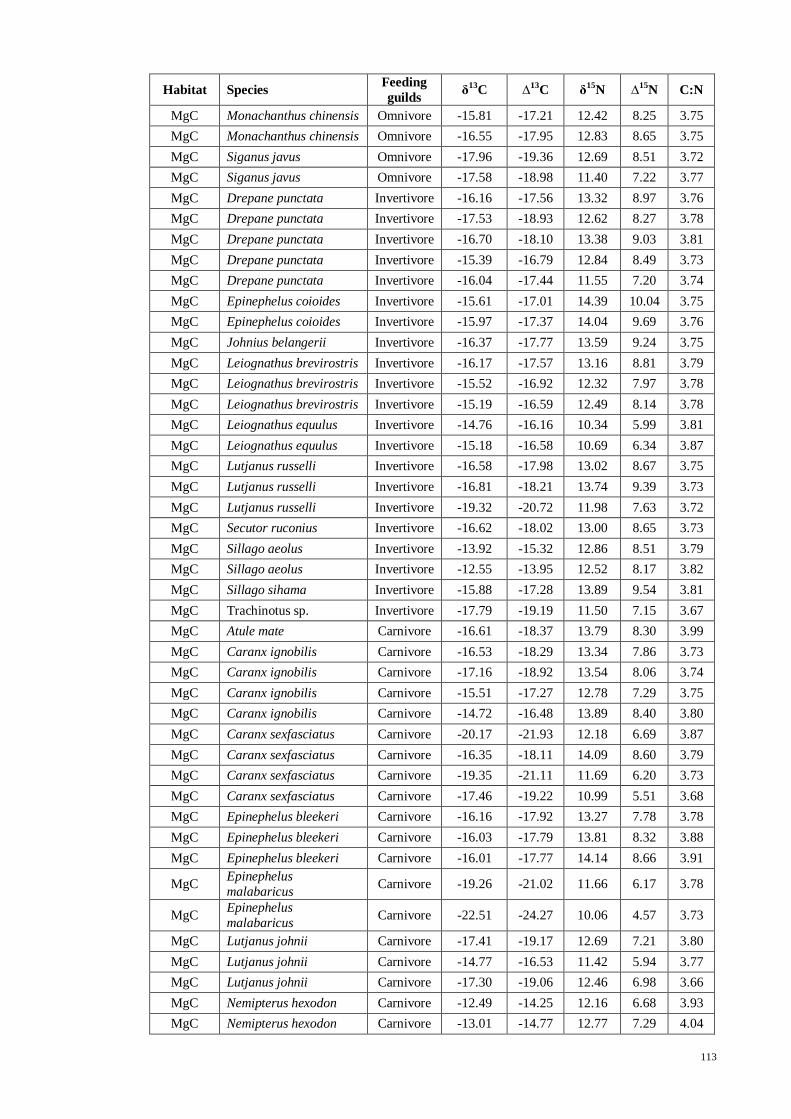
113

Habitat Species Feeding

guilds δ

13C ∆

13C δ

15N ∆

15N C:N

MgC Monachanthus chinensis Omnivore -15.81 -17.21 12.42 8.25 3.75

MgC Monachanthus chinensis Omnivore -16.55 -17.95 12.83 8.65 3.75

MgC Siganus javus Omnivore -17.96 -19.36 12.69 8.51 3.72

MgC Siganus javus Omnivore -17.58 -18.98 11.40 7.22 3.77

MgC Drepane punctata Invertivore -16.16 -17.56 13.32 8.97 3.76

MgC Drepane punctata Invertivore -17.53 -18.93 12.62 8.27 3.78

MgC Drepane punctata Invertivore -16.70 -18.10 13.38 9.03 3.81

MgC Drepane punctata Invertivore -15.39 -16.79 12.84 8.49 3.73

MgC Drepane punctata Invertivore -16.04 -17.44 11.55 7.20 3.74

MgC Epinephelus coioides Invertivore -15.61 -17.01 14.39 10.04 3.75

MgC Epinephelus coioides Invertivore -15.97 -17.37 14.04 9.69 3.76

MgC Johnius belangerii Invertivore -16.37 -17.77 13.59 9.24 3.75

MgC Leiognathus brevirostris Invertivore -16.17 -17.57 13.16 8.81 3.79

MgC Leiognathus brevirostris Invertivore -15.52 -16.92 12.32 7.97 3.78

MgC Leiognathus brevirostris Invertivore -15.19 -16.59 12.49 8.14 3.78

MgC Leiognathus equulus Invertivore -14.76 -16.16 10.34 5.99 3.81

MgC Leiognathus equulus Invertivore -15.18 -16.58 10.69 6.34 3.87

MgC Lutjanus russelli Invertivore -16.58 -17.98 13.02 8.67 3.75

MgC Lutjanus russelli Invertivore -16.81 -18.21 13.74 9.39 3.73

MgC Lutjanus russelli Invertivore -19.32 -20.72 11.98 7.63 3.72

MgC Secutor ruconius Invertivore -16.62 -18.02 13.00 8.65 3.73

MgC Sillago aeolus Invertivore -13.92 -15.32 12.86 8.51 3.79

MgC Sillago aeolus Invertivore -12.55 -13.95 12.52 8.17 3.82

MgC Sillago sihama Invertivore -15.88 -17.28 13.89 9.54 3.81

MgC Trachinotus sp. Invertivore -17.79 -19.19 11.50 7.15 3.67

MgC Atule mate Carnivore -16.61 -18.37 13.79 8.30 3.99

MgC Caranx ignobilis Carnivore -16.53 -18.29 13.34 7.86 3.73

MgC Caranx ignobilis Carnivore -17.16 -18.92 13.54 8.06 3.74

MgC Caranx ignobilis Carnivore -15.51 -17.27 12.78 7.29 3.75

MgC Caranx ignobilis Carnivore -14.72 -16.48 13.89 8.40 3.80

MgC Caranx sexfasciatus Carnivore -20.17 -21.93 12.18 6.69 3.87

MgC Caranx sexfasciatus Carnivore -16.35 -18.11 14.09 8.60 3.79

MgC Caranx sexfasciatus Carnivore -19.35 -21.11 11.69 6.20 3.73

MgC Caranx sexfasciatus Carnivore -17.46 -19.22 10.99 5.51 3.68

MgC Epinephelus bleekeri Carnivore -16.16 -17.92 13.27 7.78 3.78

MgC Epinephelus bleekeri Carnivore -16.03 -17.79 13.81 8.32 3.88

MgC Epinephelus bleekeri Carnivore -16.01 -17.77 14.14 8.66 3.91

MgC Epinephelus

malabaricus Carnivore -19.26 -21.02 11.66 6.17 3.78

MgC Epinephelus

malabaricus Carnivore -22.51 -24.27 10.06 4.57 3.73

MgC Lutjanus johnii Carnivore -17.41 -19.17 12.69 7.21 3.80

MgC Lutjanus johnii Carnivore -14.77 -16.53 11.42 5.94 3.77

MgC Lutjanus johnii Carnivore -17.30 -19.06 12.46 6.98 3.66

MgC Nemipterus hexodon Carnivore -12.49 -14.25 12.16 6.68 3.93

MgC Nemipterus hexodon Carnivore -13.01 -14.77 12.77 7.29 4.04

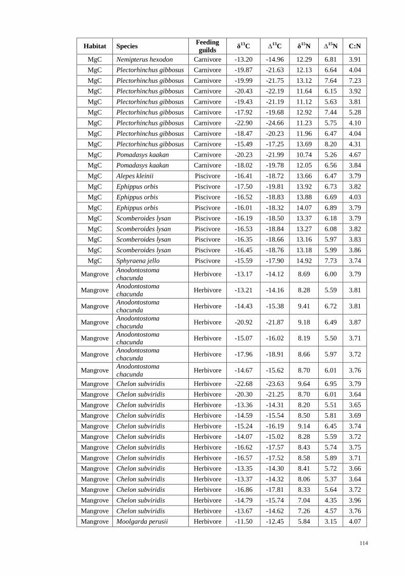
114

Habitat Species Feeding

guilds δ

13C ∆

13C δ

15N ∆

15N C:N

MgC Nemipterus hexodon Carnivore -13.20 -14.96 12.29 6.81 3.91

MgC Plectorhinchus gibbosus Carnivore -19.87 -21.63 12.13 6.64 4.04

MgC Plectorhinchus gibbosus Carnivore -19.99 -21.75 13.12 7.64 7.23

MgC Plectorhinchus gibbosus Carnivore -20.43 -22.19 11.64 6.15 3.92

MgC Plectorhinchus gibbosus Carnivore -19.43 -21.19 11.12 5.63 3.81

MgC Plectorhinchus gibbosus Carnivore -17.92 -19.68 12.92 7.44 5.28

MgC Plectorhinchus gibbosus Carnivore -22.90 -24.66 11.23 5.75 4.10

MgC Plectorhinchus gibbosus Carnivore -18.47 -20.23 11.96 6.47 4.04

MgC Plectorhinchus gibbosus Carnivore -15.49 -17.25 13.69 8.20 4.31

MgC Pomadasys kaakan Carnivore -20.23 -21.99 10.74 5.26 4.67

MgC Pomadasys kaakan Carnivore -18.02 -19.78 12.05 6.56 3.84

MgC Alepes kleinii Piscivore -16.41 -18.72 13.66 6.47 3.79

MgC Ephippus orbis Piscivore -17.50 -19.81 13.92 6.73 3.82

MgC Ephippus orbis Piscivore -16.52 -18.83 13.88 6.69 4.03

MgC Ephippus orbis Piscivore -16.01 -18.32 14.07 6.89 3.79

MgC Scomberoides lysan Piscivore -16.19 -18.50 13.37 6.18 3.79

MgC Scomberoides lysan Piscivore -16.53 -18.84 13.27 6.08 3.82

MgC Scomberoides lysan Piscivore -16.35 -18.66 13.16 5.97 3.83

MgC Scomberoides lysan Piscivore -16.45 -18.76 13.18 5.99 3.86

MgC Sphyraena jello Piscivore -15.59 -17.90 14.92 7.73 3.74

Mangrove Anodontostoma

chacunda Herbivore -13.17 -14.12 8.69 6.00 3.79

Mangrove Anodontostoma

chacunda Herbivore -13.21 -14.16 8.28 5.59 3.81

Mangrove Anodontostoma

chacunda Herbivore -14.43 -15.38 9.41 6.72 3.81

Mangrove Anodontostoma

chacunda Herbivore -20.92 -21.87 9.18 6.49 3.87

Mangrove Anodontostoma chacunda

Herbivore -15.07 -16.02 8.19 5.50 3.71

Mangrove Anodontostoma

chacunda Herbivore -17.96 -18.91 8.66 5.97 3.72

Mangrove Anodontostoma

chacunda Herbivore -14.67 -15.62 8.70 6.01 3.76

Mangrove Chelon subviridis Herbivore -22.68 -23.63 9.64 6.95 3.79

Mangrove Chelon subviridis Herbivore -20.30 -21.25 8.70 6.01 3.64

Mangrove Chelon subviridis Herbivore -13.36 -14.31 8.20 5.51 3.65

Mangrove Chelon subviridis Herbivore -14.59 -15.54 8.50 5.81 3.69

Mangrove Chelon subviridis Herbivore -15.24 -16.19 9.14 6.45 3.74

Mangrove Chelon subviridis Herbivore -14.07 -15.02 8.28 5.59 3.72

Mangrove Chelon subviridis Herbivore -16.62 -17.57 8.43 5.74 3.75

Mangrove Chelon subviridis Herbivore -16.57 -17.52 8.58 5.89 3.71

Mangrove Chelon subviridis Herbivore -13.35 -14.30 8.41 5.72 3.66

Mangrove Chelon subviridis Herbivore -13.37 -14.32 8.06 5.37 3.64

Mangrove Chelon subviridis Herbivore -16.86 -17.81 8.33 5.64 3.72

Mangrove Chelon subviridis Herbivore -14.79 -15.74 7.04 4.35 3.96

Mangrove Chelon subviridis Herbivore -13.67 -14.62 7.26 4.57 3.76

Mangrove Moolgarda perusii Herbivore -11.50 -12.45 5.84 3.15 4.07

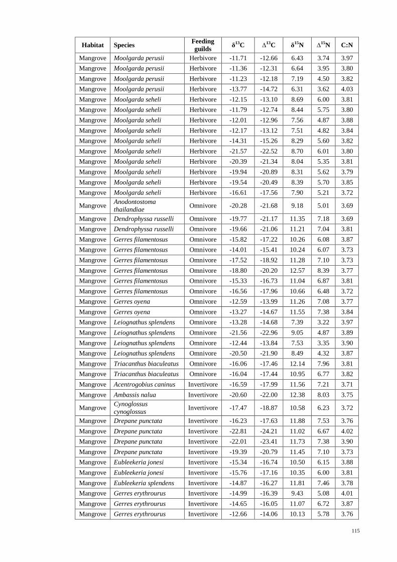
115

Habitat Species Feeding

guilds δ

13C ∆

13C δ

15N ∆

15N C:N

Mangrove Moolgarda perusii Herbivore -11.71 -12.66 6.43 3.74 3.97

Mangrove Moolgarda perusii Herbivore -11.36 -12.31 6.64 3.95 3.80

Mangrove Moolgarda perusii Herbivore -11.23 -12.18 7.19 4.50 3.82

Mangrove Moolgarda perusii Herbivore -13.77 -14.72 6.31 3.62 4.03

Mangrove Moolgarda seheli Herbivore -12.15 -13.10 8.69 6.00 3.81

Mangrove Moolgarda seheli Herbivore -11.79 -12.74 8.44 5.75 3.80

Mangrove Moolgarda seheli Herbivore -12.01 -12.96 7.56 4.87 3.88

Mangrove Moolgarda seheli Herbivore -12.17 -13.12 7.51 4.82 3.84

Mangrove Moolgarda seheli Herbivore -14.31 -15.26 8.29 5.60 3.82

Mangrove Moolgarda seheli Herbivore -21.57 -22.52 8.70 6.01 3.80

Mangrove Moolgarda seheli Herbivore -20.39 -21.34 8.04 5.35 3.81

Mangrove Moolgarda seheli Herbivore -19.94 -20.89 8.31 5.62 3.79

Mangrove Moolgarda seheli Herbivore -19.54 -20.49 8.39 5.70 3.85

Mangrove Moolgarda seheli Herbivore -16.61 -17.56 7.90 5.21 3.72

Mangrove Anodontostoma

thailandiae Omnivore -20.28 -21.68 9.18 5.01 3.69

Mangrove Dendrophyssa russelli Omnivore -19.77 -21.17 11.35 7.18 3.69

Mangrove Dendrophyssa russelli Omnivore -19.66 -21.06 11.21 7.04 3.81

Mangrove Gerres filamentosus Omnivore -15.82 -17.22 10.26 6.08 3.87

Mangrove Gerres filamentosus Omnivore -14.01 -15.41 10.24 6.07 3.73

Mangrove Gerres filamentosus Omnivore -17.52 -18.92 11.28 7.10 3.73

Mangrove Gerres filamentosus Omnivore -18.80 -20.20 12.57 8.39 3.77

Mangrove Gerres filamentosus Omnivore -15.33 -16.73 11.04 6.87 3.81

Mangrove Gerres filamentosus Omnivore -16.56 -17.96 10.66 6.48 3.72

Mangrove Gerres oyena Omnivore -12.59 -13.99 11.26 7.08 3.77

Mangrove Gerres oyena Omnivore -13.27 -14.67 11.55 7.38 3.84

Mangrove Leiognathus splendens Omnivore -13.28 -14.68 7.39 3.22 3.97

Mangrove Leiognathus splendens Omnivore -21.56 -22.96 9.05 4.87 3.89

Mangrove Leiognathus splendens Omnivore -12.44 -13.84 7.53 3.35 3.90

Mangrove Leiognathus splendens Omnivore -20.50 -21.90 8.49 4.32 3.87

Mangrove Triacanthus biaculeatus Omnivore -16.06 -17.46 12.14 7.96 3.81

Mangrove Triacanthus biaculeatus Omnivore -16.04 -17.44 10.95 6.77 3.82

Mangrove Acentrogobius caninus Invertivore -16.59 -17.99 11.56 7.21 3.71

Mangrove Ambassis nalua Invertivore -20.60 -22.00 12.38 8.03 3.75

Mangrove Cynoglossus

cynoglossus Invertivore -17.47 -18.87 10.58 6.23 3.72

Mangrove Drepane punctata Invertivore -16.23 -17.63 11.88 7.53 3.76

Mangrove Drepane punctata Invertivore -22.81 -24.21 11.02 6.67 4.02

Mangrove Drepane punctata Invertivore -22.01 -23.41 11.73 7.38 3.90

Mangrove Drepane punctata Invertivore -19.39 -20.79 11.45 7.10 3.73

Mangrove Eubleekeria jonesi Invertivore -15.34 -16.74 10.50 6.15 3.88

Mangrove Eubleekeria jonesi Invertivore -15.76 -17.16 10.35 6.00 3.81

Mangrove Eubleekeria splendens Invertivore -14.87 -16.27 11.81 7.46 3.78

Mangrove Gerres erythrourus Invertivore -14.99 -16.39 9.43 5.08 4.01

Mangrove Gerres erythrourus Invertivore -14.65 -16.05 11.07 6.72 3.87

Mangrove Gerres erythrourus Invertivore -12.66 -14.06 10.13 5.78 3.76

116

Habitat Species Feeding

guilds δ

13C ∆

13C δ

15N ∆

15N C:N

Mangrove Gerres erythrourus Invertivore -15.06 -16.46 10.04 5.69 3.87

Mangrove Himantura walga Invertivore -18.92 -20.32 11.51 7.16 3.49

Mangrove Ilisha melastoma Invertivore -18.57 -19.97 12.22 7.87 3.79

Mangrove Ilisha melastoma Invertivore -20.03 -21.43 11.66 7.31 3.76

Mangrove Lagocephalus lunaris Invertivore -14.03 -15.43 11.32 6.97 3.80

Mangrove Leiognathus brevirostris Invertivore -14.17 -15.57 12.43 8.08 3.75

Mangrove Leiognathus brevirostris Invertivore -16.13 -17.53 10.83 6.48 3.74

Mangrove Leiognathus brevirostris Invertivore -15.61 -17.01 10.59 6.24 3.81

Mangrove Leiognathus brevirostris Invertivore -15.21 -16.61 11.31 6.96 3.86

Mangrove Leiognathus brevirostris Invertivore -15.69 -17.09 10.89 6.54 3.88

Mangrove Lutjanus russelli Invertivore -17.83 -19.23 12.02 7.67 3.79

Mangrove Paranibea semiluctuosa Invertivore -16.18 -17.58 11.99 7.64 3.77

Mangrove Platycephalidae Invertivore -16.74 -18.14 9.25 4.90 3.83

Mangrove Pseudotriacanthus

strigilifer Invertivore -15.14 -16.54 12.08 7.73 3.75

Mangrove Sillago sihama Invertivore -14.95 -16.35 11.20 6.85 3.89

Mangrove Sillago sihama Invertivore -16.53 -17.93 10.78 6.43 3.76

Mangrove Sillago sihama Invertivore -16.74 -18.14 10.84 6.49 3.80

Mangrove Stolephorus indicus Invertivore -16.88 -18.28 13.19 8.84 3.76

Mangrove Tetraodon nigroviridis Invertivore -21.82 -23.22 9.95 5.60 3.69

Mangrove Thryssa hamiltonii Invertivore -15.89 -17.29 13.20 8.85 3.75

Mangrove Thryssa hamiltonii Invertivore -16.23 -17.63 14.14 9.79 3.89

Mangrove Thryssa mystax Invertivore -15.86 -17.26 13.63 9.28 3.82

Mangrove Alepes djedaba Carnivore -18.47 -20.23 11.99 6.50 3.79

Mangrove Caesio cunning Carnivore -16.43 -18.19 14.09 8.60 3.88

Mangrove Caesio cunning Carnivore -16.50 -18.26 13.20 7.71 3.76

Mangrove Caesio cunning Carnivore -16.27 -18.03 14.07 8.58 3.87

Mangrove Caesio cunning Carnivore -16.86 -18.62 13.20 7.72 3.76

Mangrove Carangoides oblongus Carnivore -16.12 -17.88 12.83 7.34 3.92

Mangrove Carangoides praeustus Carnivore -14.41 -16.17 11.23 5.74 3.77

Mangrove Carangoides praeustus Carnivore -19.23 -20.99 11.90 6.41 3.67

Mangrove Carangoides praeustus Carnivore -19.05 -20.81 12.25 6.77 3.78

Mangrove Carangoides praeustus Carnivore -16.47 -18.23 11.16 5.67 3.77

Mangrove Carangoides praeustus Carnivore -16.31 -18.07 12.42 6.93 3.81

Mangrove Carangoides praeustus Carnivore -17.79 -19.55 11.99 6.50 3.76

Mangrove Carangoides praeustus Carnivore -17.08 -18.84 12.34 6.85 3.71

Mangrove Carangoides praeustus Carnivore -18.14 -19.90 12.02 6.53 3.68

Mangrove Caranx ignobilis Carnivore -16.53 -18.29 14.08 8.59 3.72

Mangrove Caranx sexfasciatus Carnivore -19.14 -20.90 11.19 5.70 3.80

Mangrove Caranx sexfasciatus Carnivore -18.82 -20.58 11.49 6.01 3.77

Mangrove Caranx sexfasciatus Carnivore -18.21 -19.97 11.62 6.13 3.70

Mangrove Hexanematichthys sagor Carnivore -20.11 -21.87 9.44 3.96 3.72

Mangrove Pomadasys kaakan Carnivore -20.64 -22.40 9.96 4.47 3.75

Mangrove Pomadasys kaakan Carnivore -22.50 -24.26 9.33 3.84 3.76

Mangrove Pomadasys kaakan Carnivore -20.67 -22.43 10.27 4.79 3.80

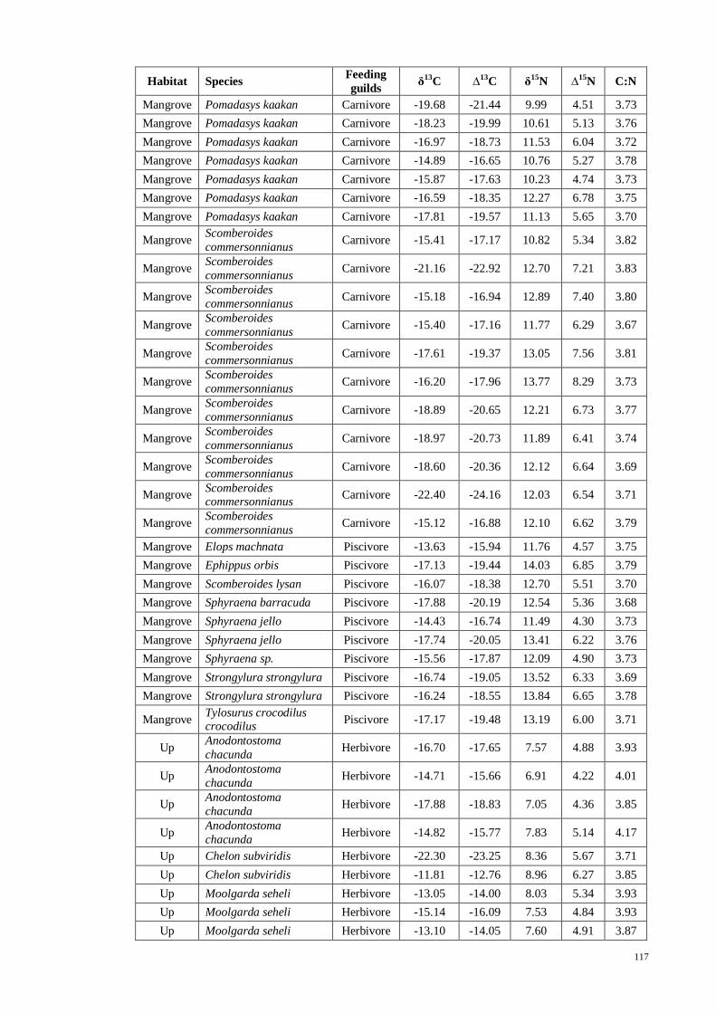
117

Habitat Species Feeding

guilds δ

13C ∆

13C δ

15N ∆

15N C:N

Mangrove Pomadasys kaakan Carnivore -19.68 -21.44 9.99 4.51 3.73

Mangrove Pomadasys kaakan Carnivore -18.23 -19.99 10.61 5.13 3.76

Mangrove Pomadasys kaakan Carnivore -16.97 -18.73 11.53 6.04 3.72

Mangrove Pomadasys kaakan Carnivore -14.89 -16.65 10.76 5.27 3.78

Mangrove Pomadasys kaakan Carnivore -15.87 -17.63 10.23 4.74 3.73

Mangrove Pomadasys kaakan Carnivore -16.59 -18.35 12.27 6.78 3.75

Mangrove Pomadasys kaakan Carnivore -17.81 -19.57 11.13 5.65 3.70

Mangrove Scomberoides

commersonnianus Carnivore -15.41 -17.17 10.82 5.34 3.82

Mangrove Scomberoides

commersonnianus Carnivore -21.16 -22.92 12.70 7.21 3.83

Mangrove Scomberoides

commersonnianus Carnivore -15.18 -16.94 12.89 7.40 3.80

Mangrove Scomberoides

commersonnianus Carnivore -15.40 -17.16 11.77 6.29 3.67

Mangrove Scomberoides

commersonnianus Carnivore -17.61 -19.37 13.05 7.56 3.81

Mangrove Scomberoides

commersonnianus Carnivore -16.20 -17.96 13.77 8.29 3.73

Mangrove Scomberoides

commersonnianus Carnivore -18.89 -20.65 12.21 6.73 3.77

Mangrove Scomberoides

commersonnianus Carnivore -18.97 -20.73 11.89 6.41 3.74

Mangrove Scomberoides

commersonnianus Carnivore -18.60 -20.36 12.12 6.64 3.69

Mangrove Scomberoides commersonnianus

Carnivore -22.40 -24.16 12.03 6.54 3.71

Mangrove Scomberoides

commersonnianus Carnivore -15.12 -16.88 12.10 6.62 3.79

Mangrove Elops machnata Piscivore -13.63 -15.94 11.76 4.57 3.75

Mangrove Ephippus orbis Piscivore -17.13 -19.44 14.03 6.85 3.79

Mangrove Scomberoides lysan Piscivore -16.07 -18.38 12.70 5.51 3.70

Mangrove Sphyraena barracuda Piscivore -17.88 -20.19 12.54 5.36 3.68

Mangrove Sphyraena jello Piscivore -14.43 -16.74 11.49 4.30 3.73

Mangrove Sphyraena jello Piscivore -17.74 -20.05 13.41 6.22 3.76

Mangrove Sphyraena sp. Piscivore -15.56 -17.87 12.09 4.90 3.73

Mangrove Strongylura strongylura Piscivore -16.74 -19.05 13.52 6.33 3.69

Mangrove Strongylura strongylura Piscivore -16.24 -18.55 13.84 6.65 3.78

Mangrove Tylosurus crocodilus crocodilus

Piscivore -17.17 -19.48 13.19 6.00 3.71

Up Anodontostoma

chacunda Herbivore -16.70 -17.65 7.57 4.88 3.93

Up Anodontostoma

chacunda Herbivore -14.71 -15.66 6.91 4.22 4.01

Up Anodontostoma

chacunda Herbivore -17.88 -18.83 7.05 4.36 3.85

Up Anodontostoma

chacunda Herbivore -14.82 -15.77 7.83 5.14 4.17

Up Chelon subviridis Herbivore -22.30 -23.25 8.36 5.67 3.71

Up Chelon subviridis Herbivore -11.81 -12.76 8.96 6.27 3.85

Up Moolgarda seheli Herbivore -13.05 -14.00 8.03 5.34 3.93

Up Moolgarda seheli Herbivore -15.14 -16.09 7.53 4.84 3.93

Up Moolgarda seheli Herbivore -13.10 -14.05 7.60 4.91 3.87

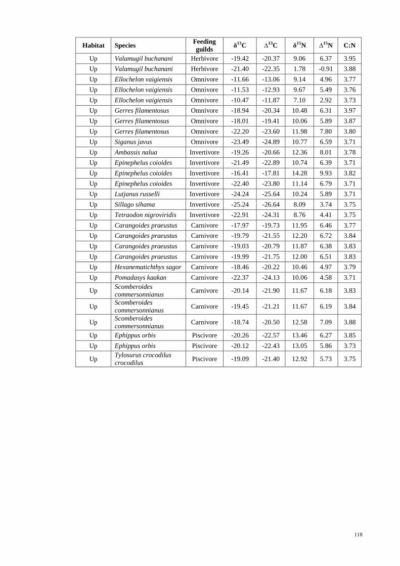
118

Habitat Species Feeding

guilds δ

13C ∆

13C δ

15N ∆

15N C:N

Up Valamugil buchanani Herbivore -19.42 -20.37 9.06 6.37 3.95

Up Valamugil buchanani Herbivore -21.40 -22.35 1.78 -0.91 3.88

Up Ellochelon vaigiensis Omnivore -11.66 -13.06 9.14 4.96 3.77

Up Ellochelon vaigiensis Omnivore -11.53 -12.93 9.67 5.49 3.76

Up Ellochelon vaigiensis Omnivore -10.47 -11.87 7.10 2.92 3.73

Up Gerres filamentosus Omnivore -18.94 -20.34 10.48 6.31 3.97

Up Gerres filamentosus Omnivore -18.01 -19.41 10.06 5.89 3.87

Up Gerres filamentosus Omnivore -22.20 -23.60 11.98 7.80 3.80

Up Siganus javus Omnivore -23.49 -24.89 10.77 6.59 3.71

Up Ambassis nalua Invertivore -19.26 -20.66 12.36 8.01 3.78

Up Epinephelus coioides Invertivore -21.49 -22.89 10.74 6.39 3.71

Up Epinephelus coioides Invertivore -16.41 -17.81 14.28 9.93 3.82

Up Epinephelus coioides Invertivore -22.40 -23.80 11.14 6.79 3.71

Up Lutjanus russelli Invertivore -24.24 -25.64 10.24 5.89 3.71

Up Sillago sihama Invertivore -25.24 -26.64 8.09 3.74 3.75

Up Tetraodon nigroviridis Invertivore -22.91 -24.31 8.76 4.41 3.75

Up Carangoides praeustus Carnivore -17.97 -19.73 11.95 6.46 3.77

Up Carangoides praeustus Carnivore -19.79 -21.55 12.20 6.72 3.84

Up Carangoides praeustus Carnivore -19.03 -20.79 11.87 6.38 3.83

Up Carangoides praeustus Carnivore -19.99 -21.75 12.00 6.51 3.83

Up Hexanematichthys sagor Carnivore -18.46 -20.22 10.46 4.97 3.79

Up Pomadasys kaakan Carnivore -22.37 -24.13 10.06 4.58 3.71

Up Scomberoides

commersonnianus Carnivore -20.14 -21.90 11.67 6.18 3.83

Up Scomberoides

commersonnianus Carnivore -19.45 -21.21 11.67 6.19 3.84

Up Scomberoides

commersonnianus Carnivore -18.74 -20.50 12.58 7.09 3.88

Up Ephippus orbis Piscivore -20.26 -22.57 13.46 6.27 3.85

Up Ephippus orbis Piscivore -20.12 -22.43 13.05 5.86 3.73

Up Tylosurus crocodilus

crocodilus Piscivore -19.09 -21.40 12.92 5.73 3.75

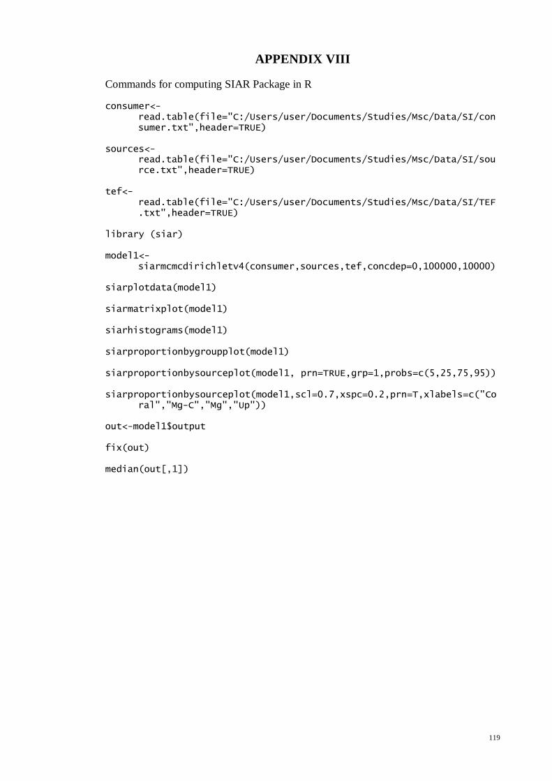
119

APPENDIX VIII

Commands for computing SIAR Package in R

consumer<-read.table(file="C:/Users/user/Documents/Studies/Msc/Data/SI/consumer.txt",header=TRUE)

sources<-

read.table(file="C:/Users/user/Documents/Studies/Msc/Data/SI/source.txt",header=TRUE)

tef<-

read.table(file="C:/Users/user/Documents/Studies/Msc/Data/SI/TEF.txt",header=TRUE)

library (siar) model1<-

siarmcmcdirichletv4(consumer,sources,tef,concdep=0,100000,10000) siarplotdata(model1) siarmatrixplot(model1) siarhistograms(model1) siarproportionbygroupplot(model1) siarproportionbysourceplot(model1, prn=TRUE,grp=1,probs=c(5,25,75,95)) siarproportionbysourceplot(model1,scl=0.7,xspc=0.2,prn=T,xlabels=c("Co

ral","Mg-C","Mg","Up")) out<-model1$output fix(out) median(out[,1])

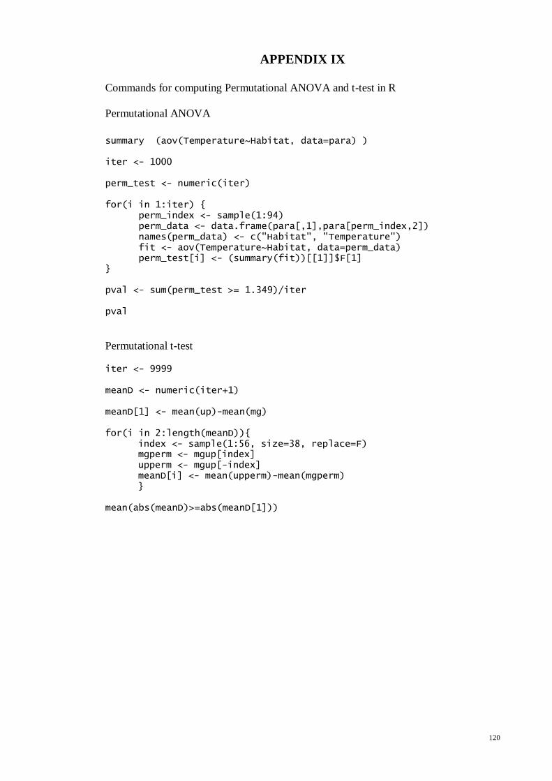
120

APPENDIX IX

Commands for computing Permutational ANOVA and t-test in R

Permutational ANOVA

summary (aov(Temperature~Habitat, data=para) ) iter <- 1000 perm_test <- numeric(iter) for(i in 1:iter) {

perm_index <- sample(1:94) perm_data <- data.frame(para[,1],para[perm_index,2]) names(perm_data) <- c("Habitat", "Temperature") fit <- aov(Temperature~Habitat, data=perm_data) perm_test[i] <- (summary(fit))[[1]]$F[1]

} pval <- sum(perm_test >= 1.349)/iter pval

Permutational t-test iter <- 9999 meanD <- numeric(iter+1) meanD[1] <- mean(up)-mean(mg) for(i in 2:length(meanD)){

index <- sample(1:56, size=38, replace=F) mgperm <- mgup[index] upperm <- mgup[-index] meanD[i] <- mean(upperm)-mean(mgperm) }

mean(abs(meanD)>=abs(meanD[1]))

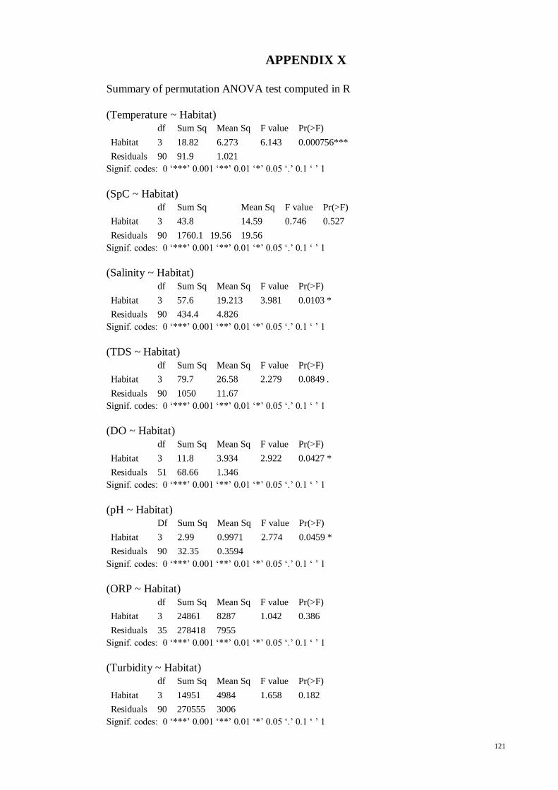
121

APPENDIX X

Summary of permutation ANOVA test computed in R

(Temperature ~ Habitat)

df Sum Sq Mean Sq F value Pr(>F)

Habitat 3 18.82 6.273 6.143 0.000756***

Residuals 90 91.9 1.021

Signif. codes: 0 ‘***’ 0.001 ‘**’ 0.01 ‘*’ 0.05 ‘.’ 0.1 ‘ ’ 1

(SpC ~ Habitat)

Signif. codes: 0 ‘***’ 0.001 ‘**’ 0.01 ‘*’ 0.05 ‘.’ 0.1 ‘ ’ 1

(Salinity ~ Habitat)

df Sum Sq Mean Sq F value Pr(>F)

Habitat 3 57.6 19.213 3.981 0.0103 *

Residuals 90 434.4 4.826

Signif. codes: 0 ‘***’ 0.001 ‘**’ 0.01 ‘*’ 0.05 ‘.’ 0.1 ‘ ’ 1

(TDS ~ Habitat)

df Sum Sq Mean Sq F value Pr(>F)

Habitat 3 79.7 26.58 2.279 0.0849 .

Residuals 90 1050 11.67

Signif. codes: 0 ‘***’ 0.001 ‘**’ 0.01 ‘*’ 0.05 ‘.’ 0.1 ‘ ’ 1

(DO ~ Habitat)

df Sum Sq Mean Sq F value Pr(>F)

Habitat 3 11.8 3.934 2.922 0.0427 *

Residuals 51 68.66 1.346

Signif. codes: 0 ‘***’ 0.001 ‘**’ 0.01 ‘*’ 0.05 ‘.’ 0.1 ‘ ’ 1

(pH ~ Habitat) Df Sum Sq Mean Sq F value Pr(>F)

Habitat 3 2.99 0.9971 2.774 0.0459 *

Residuals 90 32.35 0.3594

Signif. codes: 0 ‘***’ 0.001 ‘**’ 0.01 ‘*’ 0.05 ‘.’ 0.1 ‘ ’ 1

(ORP ~ Habitat)

df Sum Sq Mean Sq F value Pr(>F)

Habitat 3 24861 8287 1.042 0.386

Residuals 35 278418 7955

Signif. codes: 0 ‘***’ 0.001 ‘**’ 0.01 ‘*’ 0.05 ‘.’ 0.1 ‘ ’ 1

(Turbidity ~ Habitat)

df Sum Sq Mean Sq F value Pr(>F)

Habitat 3 14951 4984 1.658 0.182

Residuals 90 270555 3006

Signif. codes: 0 ‘***’ 0.001 ‘**’ 0.01 ‘*’ 0.05 ‘.’ 0.1 ‘ ’ 1

df Sum Sq Mean Sq F value Pr(>F)

Habitat 3 43.8 14.59 0.746 0.527

Residuals 90 1760.1 19.56 19.56