Fiscal Policy in the New Neoclassical Synthesis

Ludger Linnemann¤and Andreas Schaberty

December 5, 2000

¤Corresponding author. University of Cologne, Department of Economics (Staatswiss. Seminar), D-

50923 Koeln,, Germany, email: linnemann@wiso.uni-koeln.de, fax: +49/221/470-5077, tel: +49/221/470-

2999.yUniversity of Cologne.

1

Abstract: A sticky-price model is presented to analyze the cyclical e®ects of ¯scal shocks

under di®erent monetary policy regimes. Price stickiness has the consequence that changes

in the price-marginal-cost markup a®ect labor demand and can either counteract or en-

hance the wealth e®ect on labor supply. The direction of this markup e®ect depends on

the monetary policy regime; when the central bank targets money, ¯scal expansions are

contractive, while when it targets interest rates via a Taylor rule output, wages, and, ini-

tially, even consumption can rise. However, stickiness alone is not su±cient to explain the

persistent rise in consumption that recent empirical studies ¯nd.

Ludger Linnemann and Andreas Schabert

University of Cologne

Department of Economics (Staatswiss. Seminar)

Albertus Magnus Platz

D-50923 Koeln

Germany

tel +49/221/470-2999

fax +49/221/470-5077

e-mail linnemann@wiso.uni-koeln.de

2

1 Introduction

What are the e®ects of changes in government expenditure on the business cycle? His-

torically, two di®erent and mutually incompatible strands of theories have been advanced

to answer this question. Broadly characterized, there is the Keynesian tradition, on the

one hand, as captured in the familiar textbook IS-LM-Phillips-Curve model, with its focus

on the relevance of aggregate demand disturbances on cyclical conditions. Expansionary

¯scal policy, like any exogenous increase in aggregate demand, in this view allows demand

constrained ¯rms to sell more output, thus boosting income, employment, and, by the

multiplier e®ect, consumption, because the in°exibility of goods prices that prevails in

the short-run makes output demand determined; in other words, there is a non-vertical

short-run aggregate supply curve which is upward sloping because prices are temporarily

sticky and adjust only gradually, as typically captured in some version of a Phillips-Curve

speci¯cation. In the following, we will call this mechanism the `aggregate demand e®ect'

of ¯scal policy for short; see Taylor (2000) for a recent discussion.

On the other hand, the e®ects of ¯scal policy have been studied more recently in purely

real dynamic general equilibrium models with optimizing agents and fully °exible prices,

e.g. Baxter and King (1993). Here, the central mechanism by which ¯scal policy in°uences

the private economy is the negative wealth e®ect implied by the tax ¯nancing of rising

government expenditure which, with standard preferences, induces an increase in labor

supply, thus raising output and employment and depressing private consumption. This

chain of events, which we will sometimes simply abbreviate as the `wealth e®ect' in what

follows, is thoroughly di®erent from the aggregate demand e®ect story, as any change in

output and employment induced by ¯scal policy is due to the optimal response of household

labor supply. Consequently, the predictions of the neoclassical general equilibrium model

are directly opposed to those of the Keynesian theory with respect to some important

variables like wages and private consumption.

Both theories may be regarded as less than fully satisfactory due to debatable assump-

tions on which they are built. On the one hand, traditional IS-LM theorizing nowadays

seems outdated to most researchers due to its lack of conventional microfoundations and

rational expectations. On the other hand, the more recent real general equilibrium models

may be inappropriate, too, because of their neglect of any frictions in the goods or labor

market; particularly, there is a large and growing body of evidence in favor of temporary

price stickiness at business cycle frequencies (see the survey in Taylor, 1999) which points

to an important role for nominal variables to play in any business cycle theory. In related

research, namely the literature on the transmission of monetary policy, a recent consensus

model seems to have emerged, which is labelled either `New Neoclassical Synthesis' (by

Goodfriend and King, 1997), or interchangeably `New-Keynesianism' (by, among oth-

ers, Hairault and Portier, 1993), or `Neo-Monetarism' (by Kimball, 1995), or `Optimizing

IS-LM' model (by McCallum and Nelson, 1999, and Casares and McCallum, 2000); hence-

forth, we prefer the term New Neoclassical Synthesis which we will abbreviate by NNS.

The gist of this approach is the combination of an explicitly dynamic representative agent

3

optimizing general equilibrium framework with short-run nominal frictions, particularly

temporary stickiness of nominal goods prices, hence with a strong in°uence of monetary

policy on real aggregates over the business cycle. Recent research in this area, particularly

that by McCallum and Nelson (1999), has shown that much of the intuition gained from

the simple IS-LM model carries over to the NNS model as far as the e®ects of monetary

policy are concerned. Indeed, a (very) stylized version of this model has become the basic

workhorse in the literature on monetary policy; see the survey by Clarida et al. (1999).

But if price stickiness is, as perceived in a large literature, the main reason why mone-

tary policy matters, the question naturally arises whether this has any implications for the

understanding of the way ¯scal policy works. This is what the present paper intends to

contribute. One of the questions that we pursue by this approach is in how far ¯scal policy

in a typical NNS model can serve as a microfoundation for the intuition conveyed by the

IS-LM framework, thus complementing the work that McCallum and Nelson (1999) have

done for the case of monetary policy. Speci¯cally, we model a monetary economy with

a cash-in-advance constraint where optimizing households accumulate capital subject to

adjustment costs. Firms are assumed to be monopolistic competitors striving to realize a

constant markup of product prices over marginal costs, which is hampered by the presence

of the type of price stickiness originally presented in Calvo (1983), i.e. a stochastically

arriving temporary inability on the part of a subset of all ¯rms to change their output

prices as they desire in any given period. The government collects lump-sum taxes and

seignorage and uses the receipts to purchase goods; in one variant of the model these may

provide utility to the representative household, who ¯nds government consumption to be

an imperfect substitute for private consumption. Fiscal policy is modelled as a serially

correlated exogenous increase in real government expenditures. In addition, we allow a

monetary authority to endogenously react to the ¯scal stance by adjusting nominal interest

rates according to a feedback rule of the type advocated in Taylor (1993) and analyzed in

a large monetary policy literature thereafter (see, e.g., the contributions in Taylor, 1999).

Our theoretical results allow us to take a position on some unresolved issues. Particu-

larly, by considering the interaction of ¯scal with monetary policies, we obtain a possibility

to interpret some empirical results that have been reported in the literature. In principle,

empirical evidence could be expected to be useful for the purpose of distinguishing between

di®erent theories of how ¯scal policy works. This is because Keynesian and neoclassical

theories, while both predicting rising output and employment in response to temporary

¯scal expansions, have markedly di®erent implications for the responses of some other

variables, particularly for private consumption and real wages. In the Keynesian story,

private consumption should rise with government spending because income rises, due to

the aggregate demand e®ect, and exerts the usual multiplier e®ect. Real wages should rise,

too, in this view, as typical Phillips-Curves posit that because rising aggregate demand

leads to output being above its natural rate, the consequence are nominal wage increases

which in turn let goods prices rise. Both responses are predicted to be of the opposite sign

in neoclassical general equilibrium models, because the wealth e®ect depresses household

demand for leisure and private consumption, and rising labor supply leads to decreasing

4

marginal productivity of that production factor, thus lowering real wages.1 Consequently,

the empirical responses of private consumption and real wages could discriminate between

the plausibility of alternative models.

Unfortunately, the empirical literature has produced di®erent and mutually incompat-

ible results concerning the reaction of these key variables to government spending shocks.

The main reason for the opposing results seems to stem from di®erences in the empirical

methods used. There are basically two approaches: Ramey and Shapiro (1998) and the

subsequent re¯nements by Edelberg et al. (1998) and Burnside et al. (1999) consider gov-

ernment spending in speci¯c historical episodes, such as the Korean war and the Reagan

military buildup in the early 50ies and 80ies, respectively, as dictated by unique political

constellations, hence not merely being made in response to economic conditions them-

selves and thus exogenous in a statistical sense. Using dummy variables for the historical

episodes to represent exogenous ¯scal spending surges, these studies ¯nd consistently that

real wages fall while employment rises, and Ramey and Shapiro (1998) and Edelberg et

al. (1998) also ¯nd decreasing private consumption. The second empirical pocedure used

to assess the e®ects of spending shocks is the VAR innovations approach, with various

auxiliary assumptions intended to identify truly exogenous components of government ex-

penditure changes. These studies broadly produce the opposite result: Rotemberg and

Woodford (1992) and Fatas and Mihov (2000) ¯nd that most measures of real wages

increase after positive ¯scal shocks, along with output and employment, and the latter

authors also report, in accordance with Blanchard and Perotti (1999) and Mountford and

Uhlig (2000), that private consumption rises robustly with public spending.

In our model, not only can any type of real wage response to a government expenditure

shock arise as a function of the postulated degree of price stickiness, but the probability

of occurrence of a speci¯c sign of the real wage response depends on the way monetary

policy is conducted. The reason is that nominal price stickiness introduces a way for the

markup of price over marginal cost to vary inversely with employment. Thus, there is

a wedge between the real wage and the marginal product of labor which is larger when

output and employment are above normal, e.g. because a ¯scal expansion has stimulated

labor supply. Hence, price stickiness allows a second channel through which ¯scal shocks

can have e®ects on the real wage, in that the labor supply response due to the wealth e®ect

is supplemented by a labor demand e®ect due to a declining markup. This e®ect drives

the results in Rotemberg and Woodford (1992), who present a purely real model where

a countercyclical markup arises because collusion between oligopolistic ¯rms is weaker in

expansions. In our model, the result arises because some ¯rms cannot immediately adjust

prices, which seems a less controversial assumption empirically.

However, sticky prices do not only provide an alternative microfoundation for a markup

1The latter e®ect could be overridden if there were increasing returns to scale of an important size (as

assumed in Devereux et al., 1996), which is, however, empirically doubtful in the light of recent evidence

(see Basu and Fernald, 1997). The e®ect need also not arise in the neoclassical multisector model by

Ramey and Shapiro (1998).

5

e®ect in our model. More importantly, the presence of stickiness gives a role for nominal

variables to play in our story, such that the interaction of ¯scal and monetary policy

becomes crucial.2 Particularly, the markup only declines in response to a positive ¯scal

shock in our model when the central bank does not ¯x the nominal money supply, but

if it instead follows a Taylor (1993)-style feedback rule in setting the short-run nominal

interest rate in response to developments of in°ation and possibly output. The reason is

that with price stickiness the markup is negatively related to the in°ation rate, and ¯scal

expansions require falling prices when the nominal money stock is ¯xed, while they set

forth rising prices when money is endogenous and the central bank sets nominal interest

rates according to a Taylor rule. Ultimately, the e®ect of ¯scal policy on wages depends

on the monetary policy rule.

This having said, it is important to note that, even with an accomodative monetary

policy, the markup-induced labor demand e®ect just described is not identical to the

aggregate demand e®ect of ¯scal policy in the sense the term was used above to convey

the intuition for the working of the IS-LM model. On the contrary, in our model there is

no such thing as an aggregate demand e®ect because, as we demonstrate, the only reason

for output and employment to rise in the ¯rst place in response to a ¯scal shock is the

wealth e®ect on labor supply, as in the purely neoclassical model by Baxter and King

(1993). Switching o® the wealth e®ect leads to a model where ¯scal policy has no e®ect

other than crowding out private consumption one for one, leaving output unaltered. This

is the `neoclassical' side of the model, and it is entirely una®ected by the degree of price

stickiness, as well as by di®erent monetary policy rules.

One important consequence of this is that our NNS model is in con°ict with much of

the empirical evidence in that it cannot generally produce a positive reaction of private

consumption to government spending shocks. In a model where events are driven by the

wealth e®ect, private consumption should be expected to fall when public consumption

rises, as the representative agent feels having become poorer. We discuss two possibilities

to overturn this e®ect and thus to produce a positive consumption response: one is through

the Taylor rule-style monetary policy, by which endogenously expanding nominal money

exerts a counterbalancing e®ect on private consumption for some parameter constellations;

basically, when the central bank sets interest rates according to the Taylor rule, it provides

endogenous seignorage to the government which alleviates the e®ects from the ¯nancing

side of the budget expansion on private consumption partially. However, this e®ect is

not very strong in our model and can, at most, make private consumption rise in the

¯rst period following the spending shock, before the wealth e®ect again dominates. The

second possibility is to have public consumption enter the representative household's utility

function; indeed, we present a version of our model where private and public consumption

both provide utility and the elasticity of substitution between the two is constant and

2Though we emphasize the policy interaction, it should be noted that the paper is not intended to

add to the recent literature on the ¯scal theory of price determination (see, e.g., Woodford, 1994, Sims,

1994, Canozeri et al., 1998). In contrast to this approach, we apply a conventional Ricardian regime and

disregard any further restrictions on ¯scal policy.

6

¯nite. If the elasticity of substitution is below some speci¯ed value, an increase in public

spending can raise the marginal utility of private consumption, which will consequently

rise, too. However, a low elasticity of substitution implies a comparatively strong wealth

e®ect, hence relatively large additional labor input and strongly diminishing returns, which

put pressure on wages. For our preferred parametrization, no degree of price stickiness and

hence no induced markup decline is large enough to o®set this in°uence. As a consequence,

while the model can separately explain why real wages or consumption rise in response to

¯scal shocks, it cannot explain why they rise both. Thus, in sum, though equipped with

some features prominent in the Keynesian literature, the way ¯scal shocks work in our

NNS model is fundamentally more reminiscent of the neoclassical story.

The rest of this paper is organized as follows. Section 2 describes the model and, in

section 2.5, its parameterization, and section 3 presents the results by displaying impulse

responses and some sensitivity analysis with respect to important parameters. In order

to clearly work out the dependance of results on di®erent assumptions, we ¯rst explore in

section 3.1 the case of ¯scal policy with a central bank that exogenously ¯xes the nominal

money stock, and then do the same for the case of the central bank following a Taylor rule

in section 3.2. Section 4 concludes.

2 The Model

In this section we present a sticky price model which allows the analysis of ¯scal policy

shocks. The latter are identi¯ed with innovations to government expenditures which are

¯nanced in a lump-sum fashion. Money demand is introduced via a cash-in-advance

constraint. Firms are assumed to be monopolistically competitive and to adjust prices

according to Calvo's (1983) price staggering formulation. We further introduce adjustment

costs of capital as to generate reasonable investment reactions (see Casares and McCallum,

2000). Monetary policy is speci¯ed either as exogenous money growth or by a Taylor rule.

2.1 Households

Throughout the paper, nominal variables are denoted by upper-case letters, while real

variables are denoted by lower-case letters. The typical household is in¯nitely lived, with

preferences given by the expected value of a discounted stream of instantaneous utility

u (:) :

E0

" 1X

t=0

¯tu (cpt ; 1 ¡ lt)

#; ¯ 2 (0; 1); (1)

where E0 is the expectation operator conditional on the time 0 information set and ¯

is the discount factor. Instantaneous utility u (:) depends on a Cobb-Douglas bundle of

private consumption cp and leisure 1 ¡ l, where l is working time. We assume constant

relative risk aversion (CRRA):

u (cpt ; 1 ¡ lt) =[(cpt )

°(1 ¡ lt)1¡° ]1¡¾ ¡ 1

1 ¡ ¾; ° 2 (0; 1); 0 · µ · 1: (2)

7

At the beginning of period t; the representative household owns the entire stock of money

Mt in the economy. It must decide how much of this cash holdings to keep for contempo-

raneous consumption expenditures:

Ptcpt · Mt + Pt¿t; (3)

where P and ¿ denote the aggregate price level and lump-sum government transfers, re-

spectively. The cash-in-advance constraint in (3) implies that only investment is a credit

goods in this economy. This ensures that, in a variant to be explored later, when gov-

ernment expenditures enter the utility function, they are treated perfectly symmetrically

to private consumption in that they are included in the cash-in-advance constraint. The

household receives dividends ­ and the rental rate r on physical capital k as additional

°ows from monopolistically competitive ¯rms indexed by i 2 (0; 1). In period t the house-

hold chooses consumption cpt and investment expenditures et, nominal money holdings

Mt+1, and nominal riskless one-period pure discount bond holdings (1 + it+1)¡1Bt+1.

Mt+1 + (1 + it+1)¡1 Bt+1 (4)

=Ptrtkt + Bt + Mt + Pt¿t ¡ Pt(cpt + et) +

Z 1

0­itdi:

The household maximizes (1) subject to its cash-in-advance constraint (3), its budget

constraint (4), and the following condition for the accumulation of physical capital:

kt+1 = ©

µetkt

¶kt + (1 ¡ ±) kt; (5)

where ± denotes the depreciation rate of capital and ©(:) the adjustment cost function.3

This function is identical to the one used in, e.g., Bernanke et al. (1999), and is increasing

and concave. Accordingly, investment expenditures e yield a gross output of new capital

goods © (e=k) k: The inclusion of adjustment costs permits to analyze the cyclical behavior

of the price q of physical capital.4 The household's ¯rst order conditions for private

consumption, labor supply, investment expenditures and for physical capital are given by

¸t = °

£(cpt )

°(1 ¡ lt)1¡°

¤1¡¾

cpt (1 + it); (6)

wt¸t = (1 ¡ °)

£(cpt )

° (1 ¡ lt)1¡°¤1¡¾

(1 ¡ lt); (7)

¸t¯

= Et

·¸t+1

1 + it+1¼t+1

¸; (8)

qt = ©0µ

etkt

¶¡1; (9)

3The introduction of a similar adjustment cost function is suggested by Casares and McCallum (2000)

in order to generate reasonable investment responses in a sticky price model.4The function © is chosen to obtain a steady state value of the capital price q equal to one.

8

qt¯

= Et

·¸t+1¸t

µrt+1 + qt+1

µ©

µet+1kt+1

¶¡ ©0

et+1kt+1

+ (1 ¡ ±)

¶¶¸; (10)

where ¸ and ¼ denote the Lagrange multiplier for the budget constraint and the gross

in°ation rate, respectively. Furthermore, in an optimum the cash-in-advance constraint

(3) holds with equality for i > 0. Regarding the household's assets, the optimal choices

must also satisfy the following transversality conditions:

limt!1

¯tuctxt = 0; for x = k;m; b. (11)

2.2 Production

The ¯nal good which is consumed and invested in the stock of physical capital is an

aggregate of a continuum of di®erentiated goods produced by monopolistically competitive

¯rms indexed with i 2 (0; 1) . The aggregator of di®erentiated goods is de¯ned as follows:

yt =

·Z 1

0y(²¡1)²

it di

¸ ²²¡1

; with ² > 1; (12)

where y is the number of units of the ¯nal good, yi the amount produced by ¯rm i, and

² the constant elasticity of substitution between these di®erentiated goods. Let Pi and P

denote the price of good i set by ¯rm i and the price index for the ¯nal good. The demand

for each di®erentiated good is derived by minimizing the total costs of obtaining y subject

to (12):

yit =µ

PitPt

¶¡²yt: (13)

Hence, the demand for good i increases with aggregate output and decreases in its relative

price. For the price index P of the ¯nal good cost minimization implies

Pt =

·Z 1

0P(1¡²)it di

¸ 11¡²

: (14)

A monopolistically competitive ¯rm i produces good i using labor and physical capital

according to the following technology with ¯xed costs of production · :

yit =

(k®itl

1¡®it ¡ ·; if k®itl

1¡®it > ·

0 otherwisewith 0 < ® < 1; (15)

Entry and exit into the production sector is ruled out; in the steady state, there will be

zero pro¯ts because we impose a scale elasticity equal to the markup such that any excess

of revenue over factor costs will be absorbed by ¯xed costs. The ¯rms rent labor and

capital in perfectly competitive factor markets. Cost minimization for given aggregate

prices leads to real marginal costs mc which only depend on the real factor prices:

mct(wt; rt) = ®¡®(1 ¡ ®)¡(1¡®)w1¡®t r®t : (16)

9

We introduce a nominal stickiness in form of staggered price setting as developed by Calvo

(1983). Each period ¯rms may reset their prices with the probability 1 ¡ Á independent

of the time elapsed since the last price setting. The fraction Á of ¯rms are assumed to

adjust their previous period's prices according to the following simple rule:

Pit = ¼Pit¡1; (17)

where ¼ denotes the average of the in°ation rate ¼t = Pt=Pt¡1. In each period a measure

1 ¡Á of randomly selected ¯rms set new prices ePit in order to maximize the value of their

shares

maxePit

Et

" 1X

s=0

(¯Á)s #t;t+s³¼s ePityit+s ¡ Pt+smct+s(yit+s + ·)

´#; (18)

subject to yit+s =³¼s ePit

´¡²P ²t+syt+s.

Since the ¯rms are owned by the households, the weights #t;t+s of dividend payments con-

sist of the marginal utilities of consumption: #t;t+s = ¸t+s¸t

PtPt+s

. The ¯rst order condition

for the optimal price setting of °ex-price producers is given by

ePit =²

² ¡ 1

P1s=0 (¯Á)s Et

h#t;t+syt+sP

²+1t+s ¼¡²smct+s

i

P1s=0 (¯Á)sEt

h#t;t+syt+sP

²t+s¼

(1¡²)si : (19)

Using the simple price rule for the fraction Á of the ¯rms (17), the price index for the ¯nal

good as de¯ned in (14) evolves recursively over time

Pt =hÁ (¼Pt¡1)

1¡² + (1 ¡ Á) eP 1¡²t

i 11¡² : (20)

In the case of °exible prices (Á = 0) we obtain: Pit = Ptmct²=(²¡1): Hence, in a symmetric

equilibrium real marginal costs mc are constant over time when prices are °exible (mct =

(² ¡ 1)=²), while they vary in the sticky price version of the model. In the latter case the

in°ation rate evolves according to

b¼t = (1 ¡ Á)(1 ¡ ¯Á)Á¡1 cmct + ¯Et[b¼t+1];

here and in what follows for any variable x the notation bxt means the percent deviation of

xt from its steady state value xt : bxt = log(xt=xt). At the end of the period the nominal

pro¯ts ­it = Pityit ¡Ptmct(yit + ·) of ¯rm i are distributed to the household which owns

the ¯rm. All ¯rms face the same identical production technology and the same costs for

their factor inputs. In view of this symmetry the cost minimizing factor demand schedules

can be written in aggregate quantities

wt = mct (1 ¡ ®) k®t l¡®t ; (21)

rt = mct®k®¡1t l1¡®t : (22)

10

2.3 Fiscal and Monetary Policies

We consider two kinds of public liabilities, i.e. monetary balances and one-period discount

bonds. That is, the amount of borrowing in period t is Eth(1 + it+1)

¡1iBt+1 and the

amount to be repaid in period t+1 is Bt+1. The revenues of issuing public liabilities (debt

and money) net of government spending g is transferred in a lump-sum way (¿ ) to the

households. The government's budget constraint is given by

Pt¿t + Ptgt + Mt + Bt = (1 + it+1)¡1 Bt+1 + Mt+1: (23)

We set the amount of bonds equal to zero in every period. Hence, the government's

period-by-period budget constraint (23) can then be rewritten as

Pt(¿t + gt) = Mt+1 ¡ Mt: (24)

We assume that the monetary authority sets the short run nominal interest rate according

to a Taylor rule.bit = ½ibit¡1 + ½¼b¼t¡t + ½ybyt¡1: (25)

The occurrence of lagged values of the deviations of the variables on the right hand side

re°ects the critique made by McCallum (1999) that for a policy rule to be operational

the central bank should in fact be able to observe the variables it is assumed to respond

to before it comes to making decisions; Taylor rules with lagged variables are analyzed

in Rotemberg and Woodford (1999), too. Alternatively, we assume that the monetary

authority directly controls the growth rate  of the monetary aggregate: Ât = Mt+1=Mt.

Real government expenditures follow a ¯rst order autoregressive process:

log gt = ½g log gt¡1 + (1 ¡ ½i) log g + "t; (26)

where g denotes the amount of government expenditures in steady state. The autoregres-

sive parameter ½g is between zero and one and the innovations " are i.i.d. with a constant

variance ¾2" .

2.4 Rational Expectations Equilibrium

In order to induce stationarity, the model is expressed in real terms, with mt = Mt=Pt: The

endogenous state of the economy is represented by values taken by k;m; i. We restrict our

attention to equilibria with positive values of the nominal interest rate so that the house-

hold's cash-in-advance constraint (3) always binds. A rational expectations equilibrium,

then, consists of an allocation fcpt ; et; lt; kt+1;mt+1; ¿t; gtg1t=0 and a sequence of prices and

costates f¼t; wt; rt;mct; qt; ¸tg1t=0 such that (i) the household's ¯rst order conditions (6)-

(10) together with the cash-in-advance constraint (3), the capital accumulation equation

(5) and the transversality conditions are satis¯ed; (ii) the factor demand conditions (21)

and (22) as well as the pricing equations (19) and (20) are ful¯lled; (iii) the government

budget constraint (24) is satis¯ed, while the nominal interest rate is given by the rule (25);

11

(iv) the market for ¯nal output clears: yt = cpt + et + gt:

2.5 Model Parametrization

The model's equilibrium conditions are linearized around a non-stochastic steady state

and the resulting approximate linear system is solved relying on the methods in Uhlig

(1999). For that purpose, we have to supply parameters that characterize the steady state

of the model. The values for the preference and technology parameters are fairly standard

in the business cycle literature; see, e.g., Christiano and Eichenbaum (1992). The discount

factor of households ¯ is set equal to 1:03¡0:25. The production elasticity of capital ® is

set equal to 0.36. Quarterly depreciation of physical capital ± is assigned a value of 0.0212.

Steady state labor input is equal to 0.33 implying a value of 0.2925 for the consumption

expenditure share in the utility function, °. The parameter ¾ which governs the risk

aversion of the household is set to 2.

The elasticity of the price of capital with respect to the investment ratio, ©00 ¢ ( ek )=©0;

is set to -0.25. This value is taken from Bernanke et al. (1999) who also identify monetary

policy shocks with innovations to the nominal interest rate. Following Christiano et al.

(1997), the price elasticity of demand ² is assigned a value of 6, implying a mark-up equal

to 1.2. The ¯xed cost parameter is scaled to · = y=(² ¡ 1) so that in a steady state the

elasticity of scale is equal to the markup, thus entailing zero pro¯ts. The probability for

a ¯rm to be allowed to reset its price in a given period, 1 ¡ Á; is assigned a value of 0.25.

This value is conservative with respect to the estimates by Gali and Gertler (1999) and is

consistent with an average period of three quarters between price adjustments. The long-

run share of government expenditures g=y = 21% is taken from Edelberg et al. (1998).

The parameter ½g of the AR1 process is set equal to 0.9. The steady state in°ation rate

is estimated to be 1.0189.

A well known phenomenon associated with interest rate rules is the occurrence of

real indeterminacy of rational expectation equilibria in monetary business cycle models.

As shown Kerr and King (1996), uniqueness of rational expectation equilibria crucially

depends on the state contingency of the central bank's interest rate setting behavior. Con-

ventionally, a central bank's policy is called passive (active) when the partial derivative

of the nominal interest rate rule with respect to the expected in°ation rate is less (larger)

than one. Regarding a simple expectational IS-LM model, one typically ¯nds that an

active monetary policy is required to ensure equilibrium uniqueness. What is essentially

needed for this is to raise not only the nominal interest rate but even the real interest

rate in response to higher expected in°ation. Consequently, we set the parameter ½¼

governing this response equal to 1.5 which is also suggested in Taylor's (1993) famous

discussion of interest rate feedback rules. In accordance with Christiano and Gust (1999)

and Rotemberg and Woodford (1999), our results reveal that an active policy is not suf-

¯cient for uniqueness in standard dynamic general equilibrium models and needs to be

supplemented by a high autocorrelation of nominal interest rates. In order to achieve

uniqueness, we henceforth apply a value of 0.97 for the autoregressive parameter ½i in

our interest rate rule, while ½y is set to zero. The following table gives an overview over

12

parameter choices.

Table 1: Values of Preference and Technological Parameters

Parameter Descriptions Value

® production elasticity of capital 0.36

¾ relative risk aversion 2

² substitution elasticity of di®erentiated goods 6

¯ discount rate 0.9926

± depreciation rate of physical capital 0.0212

©00 ek =©0 elasticity of capital adjustment cost ¡0.25

g=y government expenditure share 0.21

l steady state labor supply 0.33

½g autoregressive shock parameter 0.9

¼ steady state in°ation 1.0189

1 ¡ Á probability of price adjustment 0.25

½i; ½¼ ; ½y Taylor rule parameters 0.97, 1.5, 0

3 Results

We present our results by discussing impulse response functions to unanticipated govern-

ment expenditure shocks for two versions of the model which are distinguished by the way

monetary policy is conducted. Subsection 3.1 analyzes the case of an exogenous growth

path of the nominal money supply which is thus unchanged by ¯scal actions, whereafter

subsection 3.2 does the same for the case of the central bank following a Taylor rule in

setting nominal interest rates. This type of presentation is to most clearly expose our

main point, the importance of the interactions between ¯scal policy and the monetary

policy regime. In our model, this importance stems from the fact that we can distinguish

two channels by which ¯scal policy impacts on the economy: the wealth e®ect by which

¯scal policy in°uences labor supply, and the markup e®ect implied by price staggering

by which government demand shifts labor demand. When nominal money is exogenous

and constant, then, concerning the determination of output and employment, both ef-

fects counteract each other, while when the central bank sets interest rates according to a

feedback rule, they work in the same direction.

3.1 Exogenous money

In this section, we assume that the nominal money stock is constant and exogenous. In

¯gure 1, we present the model's impulse responses to an unanticipated one percent increase

in government expenditure in period one, with an autoregressive parameter of the shock

process equal to 0.9. The ¯gure gives the variables' percentage response for the ¯rst twenty

13

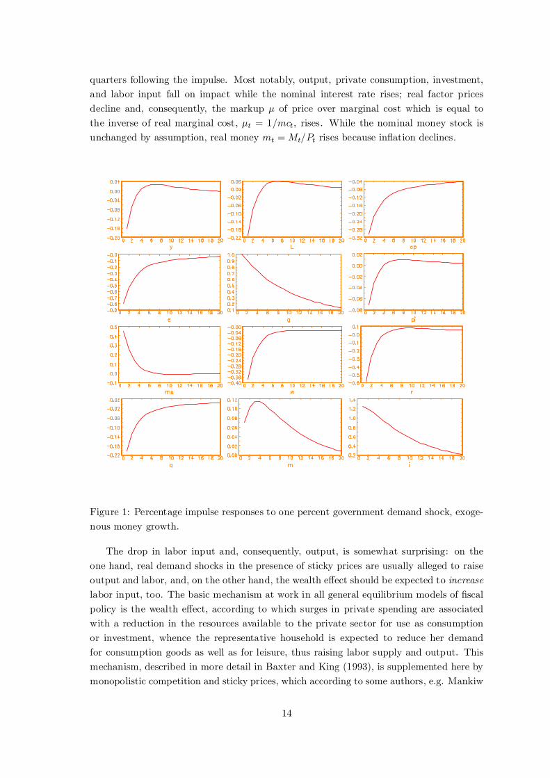
quarters following the impulse. Most notably, output, private consumption, investment,

and labor input fall on impact while the nominal interest rate rises; real factor prices

decline and, consequently, the markup ¹ of price over marginal cost which is equal to

the inverse of real marginal cost, ¹t = 1=mct, rises. While the nominal money stock is

unchanged by assumption, real money mt = Mt=Pt rises because in°ation declines.

Figure 1: Percentage impulse responses to one percent government demand shock, exoge-

nous money growth.

The drop in labor input and, consequently, output, is somewhat surprising: on the

one hand, real demand shocks in the presence of sticky prices are usually alleged to raise

output and labor, and, on the other hand, the wealth e®ect should be expected to increase

labor input, too. The basic mechanism at work in all general equilibrium models of ¯scal

policy is the wealth e®ect, according to which surges in private spending are associated

with a reduction in the resources available to the private sector for use as consumption

or investment, whence the representative household is expected to reduce her demand

for consumption goods as well as for leisure, thus raising labor supply and output. This

mechanism, described in more detail in Baxter and King (1993), is supplemented here by

monopolistic competition and sticky prices, which according to some authors, e.g. Mankiw

14

(1988), or Dixon and Lawler (1996), should provide a separate source for the expansionary

e®ects of ¯scal policy. The alleged e®ect, namely, of additional government demand in a

regime with sticky prices, is to relieve the demand constraint of monopolistically com-

petitive ¯rms, who because of their positive markups of price over marginal cost ¯nd it

pro¯table to supply more output even though they are partially unable to raise prices in

response to rising factor prices. Obviously, none of these explanations seems to ¯t the

results displayed in ¯gure 1.

The reason is that the wealth e®ect and price stickiness work in opposite directions

in this model. It remains true, in the model displayed in ¯gure 1 as in all variants to

be presented later, that the wealth e®ect is central to the understanding of ¯scal policy

e®ects. This can easily be checked (see Finn, 1998) if private consumption cpt in the utility

function of the representative agent (2) is replaced by total consumption ct as an aggregate

of private and public consumption, ct = cpt +gt, i.e. by assuming that private consumption

and government expenditures are perfect substitutes. In that case, the wealth e®ect is

switched o® and the only e®ect of a ¯scal expansion is to reduce private consumption one

for one, while all other variables are unchanged. Thus, the existence of a wealth e®ect is

necessary for the model to show any interesting responses at all. This holds for all variants

of the model we consider, irrespective of parameter choices and speci¯cations.

Given the existence of a wealth e®ect, with fully °exible prices and leisure a normal

good, one would then expect labor input to rise, thus enabling a positive output response.

This consequence of the wealth e®ect is, however, counteracted here by the presence of

price stickiness. With some prices not able to adjust immediately, the markup of price

over marginal cost, ¹t, is negatively related to in°ation, as stressed by Goodfriend and

King (1997), because changing factor prices cannot be passed instantly through to goods

prices. As the markup is the wedge between the real wage and the marginal product of

labor, the ceteris paribus e®ect of an increase in the markup is a reduction in the real wage

brought about by diminished labor demand at all wage levels. But with a given stock of

nominal money, prices must necessarily decline in this model. This can be demonstrated

by inserting the government budget constraint (24) into the cash in advance constraint

(3), resulting in

(gt + cpt ) = Mt+1=Pt: (27)

If the wealth e®ect were the only mechanism here, a rise in g initially implies falling

private consumption and rising labor supply, whence, given investment, output and the left

hand side of 27 should expand.5 Hence, with future nominal money given, the price level

must decline in order to let real money Mt+1=Pt rise, too. But this sets in motion a further

e®ect, because falling prices with staggering are equivalent to a rise in the markup of those

¯rms who are temporarily unable to decrease their output prices while the factor prices

they face decline. This markup rise is a negative labor demand e®ect in the sense just

described. As a consequence, the real wage is reduced sharply, which lowers the incentive

5The argumentmakes use of the result that the response of investment, due to the presence of adjustment

costs, is not so strongly negative that output must fall.

15

to work and thus reduces labor supply. The in°uences of labor supply and demand hence

work in opposite directions here with respect to labor input, while they mutually reinforce

each other to unambiguously lower wages.

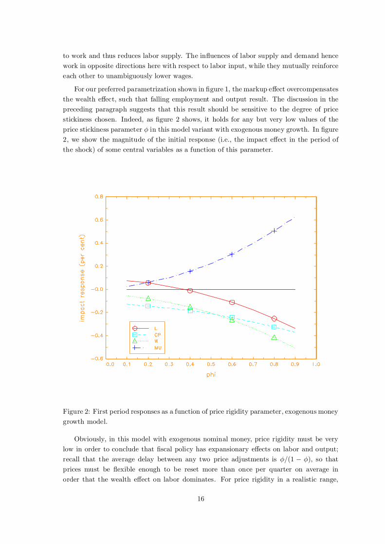
For our preferred parametrization shown in ¯gure 1, the markup e®ect overcompensates

the wealth e®ect, such that falling employment and output result. The discussion in the

preceding paragraph suggests that this result should be sensitive to the degree of price

stickiness chosen. Indeed, as ¯gure 2 shows, it holds for any but very low values of the

price stickiness parameter Á in this model variant with exogenous money growth. In ¯gure

2, we show the magnitude of the initial response (i.e., the impact e®ect in the period of

the shock) of some central variables as a function of this parameter.

Figure 2: First period responses as a function of price rigidity parameter, exogenous money

growth model.

Obviously, in this model with exogenous nominal money, price rigidity must be very

low in order to conclude that ¯scal policy has expansionary e®ects on labor and output;

recall that the average delay between any two price adjustments is Á=(1 ¡ Á), so that

prices must be °exible enough to be reset more than once per quarter on average in

order that the wealth e®ect on labor dominates. For price rigidity in a realistic range,

16

jugded by the results in Gali and Gertler (1999), the markup rises so strongly that the

resulting wage decrease discourages additional labor supply. Note, from ¯gure 2, that

private consumption decreases for any degree of the price stickiness parameter, a direct

consequence of the wealth e®ect to which we will return below.

For a realistic extent of slow price adjustment, the model variant presented so far

delivers just the opposite of what one would expect if it were truly just capturing some

modernized version of the working of IS-LM models. The very presence of price stickiness,

often alleged to be a source for large output e®ects of demand shocks, has on the con-

trary been shown to lead to output decreases for empirically plausible parameter values.

Furthermore, some other of the model's implications are in stark contrast to much of the

received empirical evidence cited in the introduction, which points to positive e®ects of

¯scal expansions on output, consumption, and real wages. Thus, the conclusion so far

is that while NNS models like ours have been found useful to give a microfoundation to

models usable for the analysis of monetary policy, the same does not seem to be true for

¯scal policy. However, this might be due to an inadequate representation of the interaction

between ¯scal and monetary policies in the model variant discussed so far. This is what

we turn to now.

3.2 Interest rate rules

The model of the preceding subsection has taken the nominal stock of money to be ex-

ogenously given and growing at a constant rate. The recent literature, however, has seen

a strongly growing occupation with explicit models of interest rate policy, where the cen-

tral bank is assumed to control the short term nominal rate according to some rule that

typically implies feedback between the state of the economy and the target rate. In this

section, we take up this issue and study the e®ects of ¯scal shocks when the central bank

follows a state contingent rule in setting interest rates. In the context of ¯scal policy, the

di®erence between the two speci¯cations of central bank behavior is crucial if there is a

friction present that makes it possible for nominal variables to in°uence the real economy,

as is the case in the present model through nominal price stickiness. If monetary policy

is conducted in terms of a feedback rule for the nominal interest rate, then the nomi-

nal money stock is endogenous, of course, and adjusts in response to disturbances like

¯scal policy. We explore the implications for the e®ects of ¯scal shocks in the following

subsections.

3.2.1 Baseline results

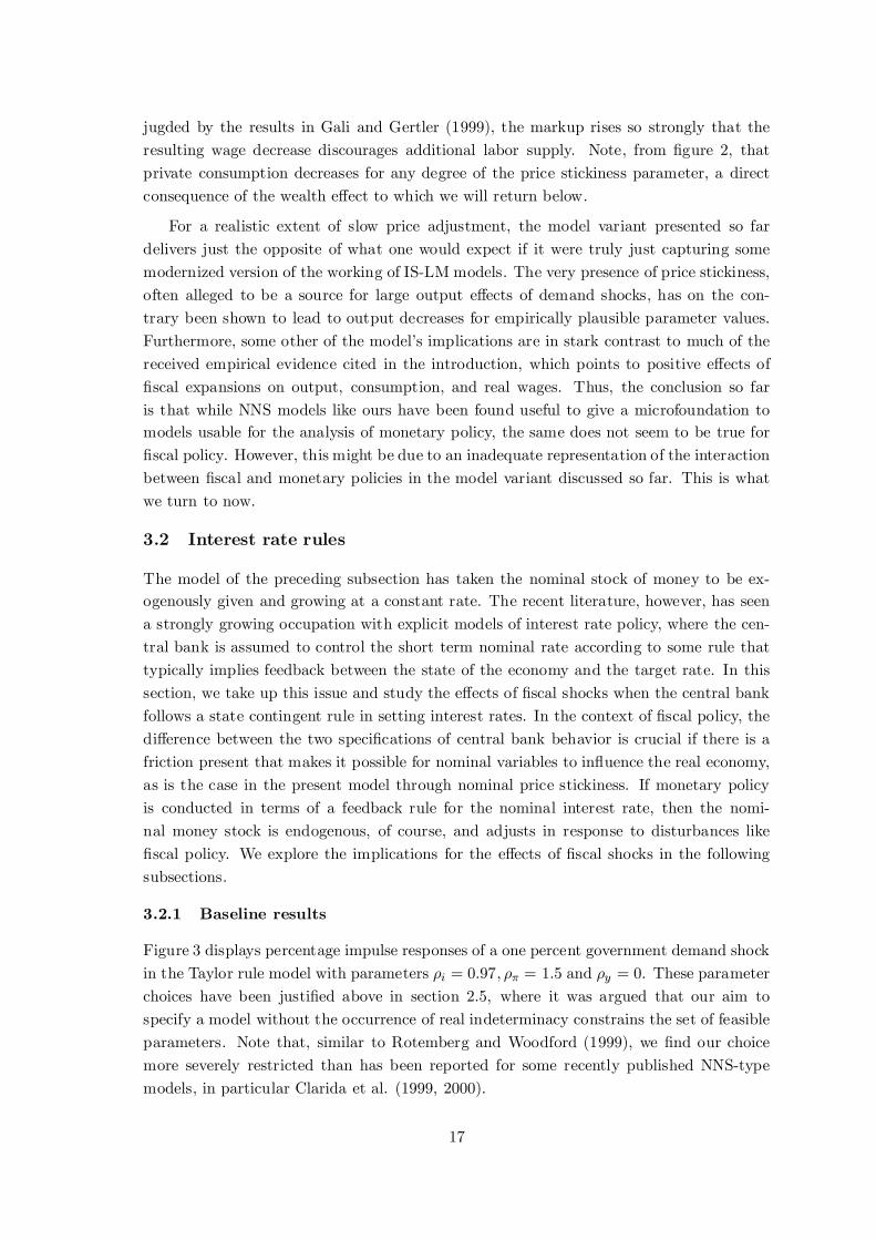
Figure 3 displays percentage impulse responses of a one percent government demand shock

in the Taylor rule model with parameters ½i = 0:97; ½¼ = 1:5 and ½y = 0. These parameter

choices have been justi¯ed above in section 2.5, where it was argued that our aim to

specify a model without the occurrence of real indeterminacy constrains the set of feasible

parameters. Note that, similar to Rotemberg and Woodford (1999), we ¯nd our choice

more severely restricted than has been reported for some recently published NNS-type

models, in particular Clarida et al. (1999, 2000).

17

Figure 3: Percentage impulse responses to one percent government demand shock, Taylor

rule model.

Obviously, results are in stark contrast to those obtained in the model with exogenous

money. In particular, the ¯scal spending shock now has a strong expansionary e®ect on

output and employment. Interestingly, even private consumption and investment rise in

the ¯rst period when the shock arrives, but afterwards their responses turn persistently

negative. The real wage and the real capital rental rate display relatively large increases,

as does real marginal cost, consequently, while in°ation rises slightly. The nominal interest

rate is increased by a very small amount only which is clearly due to the assumed interest

rate smoothing behavior of the central bank. Real money rises strongly, almost four times

as large on impact as in the case of exogenous nominal money; combined with the positive

but quantitatively small in°ation response, this shows that the nominal money stock in

the Taylor rule model is expanded strongly and about as much as output.

Why has a government demand shock so markedly di®erent e®ects in this model com-

pared to the exogenous money growth model of the previous subsection? Like before, the

explanation must start with the wealth e®ect, as there would be no response other than

crowding out of private consumption if the wealth e®ect were eliminated through the as-

18

sumption of perfect substitutability between private and public consumption. Therefore,

the initial reaction of the representative agent to a government expenditure shock is a

ceteris paribus increase in labor supply and a reduction in private consumption. But now

money is endogenous, which has the important consequence that the equilibrium price

level has to rise, so that a gradual adjustment of in°ation lowers the markup and thus

exerts an expansionary labor demand e®ect. To see this, consider again equation (27). In

the present Taylor rule model, the nominal interest rate rises by far not as much as in

the exogenous money model of the previous section, as the central bank tends to smooth

interest rates strongly. This means that private consumption falls by less than in the ¯xed

money model, such that cpt + gt is increased more; consequently, real money Mt+1=Pt has

to rise more here, too. In principle, this could be brought about by a price level that falls

more than in the constant money model. But this is impossible, since it would imply a

larger markup increase and, hence, a stronger contractive labor demand e®ect, which is in

contradiction to the statement that the output e®ect be larger than in the other model.6

Thus, the necessary increase in real money is realized through rising future nominal money.

This has the usual e®ects of an anticipated increase in the nominal money supply, most

notably an increase in the equilibrium price level and hence in in°ation. This, eventually,

reduces the markup, implying a positive labor demand e®ect. By the interaction of wealth

e®ect and markup e®ect, labor input rises unambiguosly, while real wages may rise or fall

depending on parameter values.

Particularly, the degree of price rigidity can be expected to have a decisive in°uence

here. Again, the impact e®ects of a ¯scal expansion are displayed in ¯gure 4 as a function of

the degree of price rigidity, Á. For the variables shown, the impact e®ects point in exactly

the opposite direction than was the case in the model with an exogenous money supply.

More stickiness in nominal goods prices (a higher value of Á) leads to larger responses

of labor, consumption and real wages, and to larger declines of the markup. Moreover,

although labor rises relatively strongly, this coincides for most parameter values with

rising rather than falling real wages due to the strong reduction in the markup; private

consumption, in contrast, initially falls for modest price stickiness and experiences a short-

lived ¯rst period increase only with larger values of Á, even if these are in the range found

empirically plausible by Gali and Gertler (1999).

What remains to be explained is the positive ¯rst period response of private consump-

tion. The rise in the nominal money stock has a transfer e®ect on the representative

household's wealth, thus partially o®setting the negative wealth e®ect of additional gov-

ernment spending. In other words, the combination of an increase in money demand with

a central bank that sets and smoothes nominal interest rates allows the government to

¯nance part of the expenditure shock by seignorage, which in a sticky-price model has,

ceteris paribus, the usual expansionary e®ects. Which of the opposing channels, wealth ef-

fect or seignorage e®ect, dominates the response of private consumption is thus a question

6Again, this argument equates output with the sum of private consumption and government spending,

tacitly taken as given that the investment response is too weak to alter the conclusion.

19

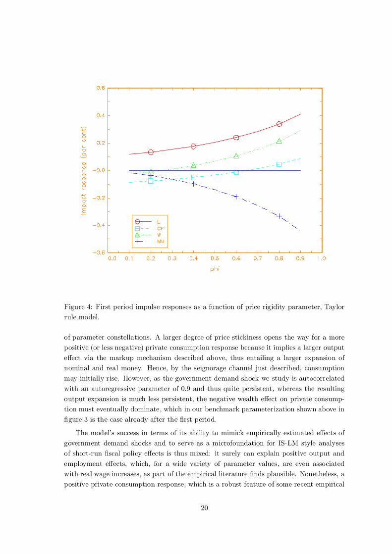
Figure 4: First period impulse responses as a function of price rigidity parameter, Taylor

rule model.

of parameter constellations. A larger degree of price stickiness opens the way for a more

positive (or less negative) private consumption response because it implies a larger output

e®ect via the markup mechanism described above, thus entailing a larger expansion of

nominal and real money. Hence, by the seignorage channel just described, consumption

may initially rise. However, as the government demand shock we study is autocorrelated

with an autoregressive parameter of 0.9 and thus quite persistent, whereas the resulting

output expansion is much less persistent, the negative wealth e®ect on private consump-

tion must eventually dominate, which in our benchmark parameterization shown above in

¯gure 3 is the case already after the ¯rst period.

The model's success in terms of its ability to mimick empirically estimated e®ects of

government demand shocks and to serve as a microfoundation for IS-LM style analyses

of short-run ¯scal policy e®ects is thus mixed: it surely can explain positive output and

employment e®ects, which, for a wide variety of parameter values, are even associated

with real wage increases, as part of the empirical literature ¯nds plausible. Nonetheless, a

positive private consumption response, which is a robust feature of some recent empirical

20

VARs, can hardly be obtained, as consumption can only rise with relatively extreme price

stickiness, and even then only for a short period of time. The next subsection analyzes

consumption in more detail.

3.2.2 Consumption and real wages.

The model is so far not able to produce a reasonably persistent positive private con-

sumption response, because the wealth e®ect of government spending which underlies its

mechanism must sooner or later dominate, at least for quite persistent shocks like the

one we speci¯ed using an autoregressive parameter for the shock process of 0.9. However,

an obvious way around this problem is to make government spending an argument of the

representative household's utility function. This is a thoroughly sensible assumption, since

governments typically do not produce only waste, but supply goods which are of value to

the household and which are, moreover, more or less substitutable with private spendings;

examples comprise schools, roads, local public utilities, etc. If, however, the household's

elasticity of substitution between private and public consumption is su±ciently low, an

increase in public spending can increase the marginal utility of private consumption and,

therefore, private consumption itself. Consider the replacement of private consumption

cpt in the utility function by a constant elasticity of substitution aggregate ct of private

consumption and government consumption gt,

ct =

·b ¢ (cpt )

( z¡1z ) + (1 ¡ b) ¢ g( z¡1z )t

¸ zz¡1

; b 2 (0; 1); z > 0;

where z is the elasticity of substitution between private and public consumption. Then,

the sign of the derivative of the marginal utility of private consumption with respect to

government consumption is equal to the sign of °(1 ¡ ¾) ¡ (z ¡ 1)=z: In the benchmark

parameterization of the model, we chose ¾ = 2 and calibrated ° just below 0.3, such that

a government demand shock will raise private consumption if the elasticity of substitution

is less than about 0.77. Figure 5 shows the impulse responses of private consumption and

the real wage to a one percent government demand shock for the benchmark parameter

choice of the preceding subsection combined with b = 0:5 and z 2 f0:3; 0:6g.

Clearly, as expected, consumption now reacts markedly positively and quite persis-

tently to the ¯scal expansion, because the utility function implies weak substitution be-

tween public and private consumption, such that the household's desire to limit changes in

the relation between the two and thus expand private spending is stronger than the wealth

e®ect which tends to reduce it. Obviously, the e®ect is the stronger the less substitutabil-

ity there is. While this is an easy method to generate positive consumption responses to

¯scal shocks, and thus to bring one of the model's properties more in line with empirical

results, ¯gure 5 also shows the °ip side of this achievement: the real wage has to fall, and

the amount of its decline is larger with a smaller elasticity of substitution; thus, the more

positive is the consumption response, the more pronouncedly negative is by implication

the real wage response.

21

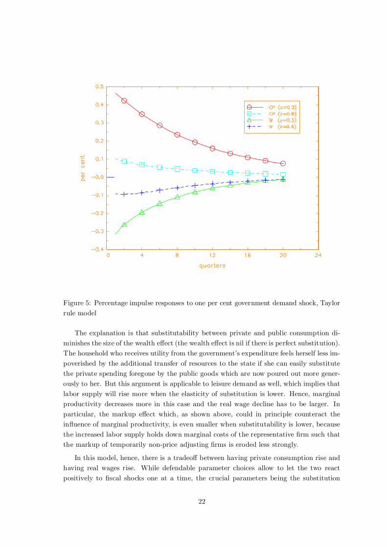
Figure 5: Percentage impulse responses to one per cent government demand shock, Taylor

rule model

The explanation is that substitutability between private and public consumption di-

minishes the size of the wealth e®ect (the wealth e®ect is nil if there is perfect substitution).

The household who receives utility from the government's expenditure feels herself less im-

poverished by the additional transfer of resources to the state if she can easily substitute

the private spending foregone by the public goods which are now poured out more gener-

ously to her. But this argument is applicable to leisure demand as well, which implies that

labor supply will rise more when the elasticity of substitution is lower. Hence, marginal

productivity decreases more in this case and the real wage decline has to be larger. In

particular, the markup e®ect which, as shown above, could in principle counteract the

in°uence of marginal productivity, is even smaller when substitutability is lower, because

the increased labor supply holds down marginal costs of the representative ¯rm such that

the markup of temporarily non-price adjusting ¯rms is eroded less strongly.

In this model, hence, there is a tradeo® between having private consumption rise and

having real wages rise. While defendable parameter choices allow to let the two react

positively to ¯scal shocks one at a time, the crucial parameters being the substitution

22

elasticity for private consumption and the degree of price stickiness for the wage, the com-

bined result of both variables rising is not possible for our speci¯cation. This, again, points

to the fact that, despite New Keynesian assumptions such as monopolistic competition

and price staggering, the model is predominantly neoclassical in that it heavily relies on

the wealth e®ect as its central mechanism. Therefore, its working is quite far detached

from what one would expect from a modernized version of IS-LM.

4 Conclusion

In this paper, we have investigated the e®ects of ¯scal policy in an environment of sticky

prices. The reason for doing so was twofold: one question we pursued was to what extent

monopolistic competition between ¯rms and staggered price adjustment makes the e®ects

of ¯scal policy look Keynesian, i.e. raise output, employment, real wages and consump-

tion temporarily. The other question was what kind of in°uence the speci¯cation of the

monetary policy regime has on the results once money begins to matter because of price

stickiness.

We ¯nd that monetary policy behavior is crucial for understanding ¯scal policy e®ects.

In particular, for our preferred parameterization of the model, ¯scal policy is only expan-

sionary at all if the central bank adheres to a Taylor rule-style policy in setting nominal

interest rates. In that case, output and employment rise, while the same is true for real

wages and private consumption, but only for a limited number of periods following the

shock. The result regarding the real wage is due to the e®ect ¯scal policy has on the

price level in our economy; when it is able to raise prices, as is the case when the central

bank accomodates money demand by targeting interest rates, then in°ation will erode

the markup and labor demand will rise at all wage levels. While this has admittedly a

Keynesian °avor, the same is not true for the private consumption, which experiences

only a one-period expansion before perstently falling; the latter result could be reversed

by making government expenditure an imperfect substitute for private consumption in

the utility function, but this works only at the expense of having ¯scal shocks strongly

depress real wages. As a result, we conclude that even with sticky prices and a monetary

authority that targets nominal interest rates, there is no aggregate demand e®ect of ¯scal

policy in our model that could remind in any precise way of the Keynesian story.

Finally, we should comment on why this result is in contrast to part of the literature.

In several recent papers, e.g. Clarida et al. (1999, 2000), a stylized version of an NNS-type

model has been presented consisting of three basic ingredients: a Taylor rule for nominal

interest rates, an 'expectational IS equation', i.e. a ¯rst order condition for consumption

coupled with market clearing, and a Phillips-curve equation, e.g. the one resulting from the

Calvo (1983)-type model that we used above, too. A graphical and verbal presentation of

the workings of such a model is given by Taylor (2000), where he emphasizes the usefulness

of a model of this type for what he calls 'new normative macroeconomics' and by which he

means the quantitative exploration of macro policies in small dynamic stochastic models.

We do not doubt the usefulness of small-scale NNS models of the three equation vari-

23

ety for the purpose of analyzing monetary policy, which is the objective in Clarida et al.

(1999, 2000). However, we think it misleading to couch discussions of ¯scal policy in the

same stylized framework, as does Taylor (2000) when he describes the working of a gov-

ernment spending shock to 'shift the AD [aggregate demand] curve'. As we demonstrated

above, the assumptions of sticky prices and a Taylor rule are not enough to produce re-

sults that deviate much from the neoclassical benchmark elaborated on by, e.g., Baxter

and King (1993) for the basic mechanism by which the model works is still the neoclas-

sical wealth e®ect on labor supply, even if in some parameter constellations, or through

endogenous monetary policy, this may sometimes be attenuated or even overcompensated.

Yet this mechanism is missing from the three equation models just cited because there

is no consideration at all of labor supply issues. Consequently, the description of ¯scal

policy e®ects in these models based on aggregate demand e®ects is misleading unless one

argues that there is an implicit assumption of underutilized labor resources which make

labor supply considerations irrelevant, as is sometimes suggested in textbook versions of

IS-LM models. In that case, however, the existence of chronic underemployment should

rather be modelled directly rather than just used as a justi¯cation for short-cutting the

way ¯scal policy works.

24

5 References

Basu, S., and J.G. Fernald, , 1997, Returns to Scale in U.S. Production: Estimates

and Implications, Journal of Political Economy, vol. 105, 249-283.

Bernanke, B.S., M. Gertler, and S. Gilchrist, 1999, The Financial Accelerator in a

Quantitative Business Cycle Framework, in: Handbook of Macroeconomics, Chapter

21, edited by J.B. Taylor and M. Woodford, Amsterdam: Elsevier.

Baxter, M., and R.G. King, 1993, Fiscal Policy in General Equilibrium, American

Economic Review, vol. 83, 315-334.

Blanchard, O.J., and R. Perotti, 1999, An Empirical Characterization of the Dy-

namic E®ects of Changes in Government Spending and Taxes on Output, Working

paper.

Burnside, C., M. Eichenbaum, and J.D.M. Fischer, 1998, Assessing the e®ects of

¯scal shocks, Working paper.

Calvo, G., 1983, Staggered Prices in a Utility-Maximizing Framework, Journal of Mon-

etary Economics, vol. 12, 383-398.

Canozeri, M., Crumby, R., and B., Diba, 1998, Is the Price Level Determined by

the Needs of Fiscal Solvency? CEPR Working Paper no. 1772.

Casares, M., and B.T. McCallum, 2000, An Optimizing IS-LM Framework with En-

dogenous Investment, NBER Working Paper, no. 7908.

Christiano, J.L., and M. Eichenbaum, 1992, Liquidity E®ects and the Monetary Trans-

mission Mechanism, American Economic Review, vol. 82, 346-53.

Christiano, J.L., M. Eichenbaum, and C. Evans, 1997, Sticky price and Limited

Participation Models of Money: A Comparison, European Economic Review, vol. 41,

1201-49.

Christiano, J.L., and G. Gust, 1999, Taylor Rules in a Limited Parizipation Model,

in: Monetary Policy Rules, edited by J.B. Taylor, University of Chicago Press.

Clarida, R., J. Gali, and M. Gertler, 1999, The Science of Monetary Policy: A New

Keynesian Perspective, Journal of Economic Literature, vol. XXXVII, 1661-1707.

Clarida, R., J. Gali, and M. Gertler, 2000, Monetary Policy Rules and Macroeco-

nomic Stability: Evidence and Some Theory, Quarterly Journal of Economics, vol.

CXL, 147-180.

Devereux, M.B., A.C. Head, and B.L. Lapham, 1996, Monopolistic Competition,

Increasing Returns, and the E®ects of Government Spending, Journal of Money,

Credit, and Banking, vol. 28, 233- 254.

25

Dixon, H., and P. Lawler, 1996, Imperfect Competition and the Fiscal Multiplier, Scan-

dinavian Journal of Economics, vol. 98, 219-231.

Edelberg, W., M. Eichenbaum, and J.D.M. Fisher, 1999, Understanding the Ef-

fects of Shocks to Government Purchases, Review of Economic Dynamics, 166-206.

Fatas, A., and I. Mihov, 2000, Fiscal Policy and Business Cycles: An Empirical Inves-

tigation, Working paper.

Finn, M.G., 1998, Cyclical E®ects of Government's employment and goods purchases,

International Economic Review, vol. 39, 635-657.

Gali, J., and M. Gertler, 1999, In°ation Dynamics: A Structural Econometric Analy-

sis, Journal of Monetary Economics, vol. 44, 195-222.

Goodfriend, M., and R.G. King, 1997, The New Neoclassical Synthesis and the Role

of Monetary Policy, NBER Macroeconomics Annual, 231-283.

Hairault, J.O., and F. Portier, 1993, Money, New-Keynesian Macroeconomics, and

the Business Cycle, European Economic Review, vol. 37, 1533-1568.

Kerr, W., and R.G. King, 1996, Limits on Interest Rate Rules in the IS Model, Fed-

eral Reseve Bank of Richmond Economic Quarterly, vol. 82, 47-75.

Kimball, M.S., 1995, The quantitative analytics of the basic neomonetarist model, Jour-

nal of Money, Credit, and Banking, vol. 27, 1241-1289.

Mankiw, N.G., 1988, Imperfect Competition and the Keynesian Cross, Economics Let-

ters, vol. 26, 7-14.

McCallum, B.T., 1999, Issues in the Design of Monetary Policy Rules, in: Handbook of

Macroeconomics, Chapter 23, edited by J.B. Taylor and M. Woodford, Amsterdam:

Elsevier.

McCallum, B.T., and E. Nelson, 1999, An Optimizing IS-LM Speci¯cation for Mon-

etary Policy and Business Cycle Analysis, Journal of Money, Credit, and Banking,

vol. 31, 296-316.

Mountford, A., and H. Uhlig, 2000, What are the E®ects of Fiscal Policy Shocks?,

Working paper.

Ramey, V.A., and M.D. Shapiro, 1998, Costly Capital Reallocation and the E®ects

of Government Spending, Carnegie-Rochester Conference Series on Public Policy,

vol. 48, 145-194.

Rotemberg, J.J., and M. Woodford, 1992, Oligopolistic Pricing and the E®ects of

Aggregate Demand on Economic Activity, Journal of Political Economy, vol. 100,

1153-1207.

26

Rotemberg, J.J., and M. Woodford, 1997, An Optimization-based Econometric Frame-

work for the Evaluation of Monetary Policy, NBER Macroeconomics Annual, 297-

346.

Rotemberg, J.J., and M. Woodford, 1999, Interest Rate Rules in an Estimated Sticky

Price Model, in: Monetary Policy Rules, edited by J.B. Taylor, University of Chicago

Press.

Sims, C., 1994, A Simple Model of the Determination of the Price Level and the Inter-

action of Monetary and Fiscal Policy, Economic Theory, vol. 4., 381-399.

Taylor, J.B., 1993, Discretion versus Policy Rules in Practice, Carnegie-Rochester Con-

ference series on Public Policy, vol. 39, 195-214.

Taylor, J.B., 1999, Staggered price and wage setting in macroeconomics, in: Handbook

of Macroeconomics, Chapter 15, edited by J.B. Taylor and M. Woodford, Amster-

dam: Elsevier.

Taylor, J.B., 2000, Reassessing Discretionary Fiscal Policy, Journal of Economic Per-

spectives, vol 14, 21-36.

Uhlig, H., 1999, A Toolkit for Analysing Nonlinear Dynamic Stochastic Models Easily,

in: Computational Methods for the Study of Dynamic Economies, edited by R.

Marimon and A. Scott, Oxford: Oxford University Press.

Woodford, M., 1994, Monetary Policy and Price Level Determinacy in a Cash-in-advance

Economy, Economic Theory, vol. 4., 345-380.

27