Fiscal Deficits and GovernmentDebt in India: Implications for

Growth and Stabilisation

C. Rangarajan* and

D.K.Srivastava**

Abstract

This paper examines the long term profile of fiscal deficit anddebt relative to GDP in India, with a view to analysing debt-deficitsustainability issues along with the considerations relevant fordetermining suitable medium and short-term fiscal policy stance. Theimpact of debt and fiscal deficit on growth and interest rates that arisesfrom their effect on saving and investment are critical in any examinationof sustainability of debt and deficit. It is argued that large structuralprimary deficits and interest payments relative to GDP have had anadverse effect on growth in recent years. The Fiscal Responsibility andBudget management Act (FRBMA) of the central government has certainpositive features. While the fiscal deficit target has been defined, itshould be considered in conjunction with a target debt-GDP ratio.Further, the central FRBMA should be supplemented by state level fiscalresponsibility legislations and an effective hard budget constraint on sub-national borrowing. There is a clear need to bring down the combineddebt-GDP ratio from its current level, which is in excess of 80 percent ofGDP. The process of adjustment can be considered in two phases:adjustment phase and stabilisation phase. In the adjustment phase,

-----------------------------------------------* Chairman, National Institute of Public Finance and Policy, New Delhi.** Senior Fellow, National Institute of Public Finance and Policy, New Delhi.Authors are thankful to Amaresh Bagchi for helpful comments on an earlierversion of the paper.

4

fiscal deficit should be reduced in each successive year until revenuedeficit, and correspondingly, government dissaving, is eliminated. In thesecond phase, fiscal deficit could be stabilised at 6 percent of GDP. Thedebt-GDP ratio would eventually stabilise at 56 percent. In this process,the ratio of interest payments to revenue receipts will fall, enabling aprogressively larger amount of primary revenue expenditure to beincurred on the social sectors.

5

Fiscal Deficits and GovernmentDebt in India: Implications for

Growth and Stabilisation

Fiscal deficits are like obesity. You can see your weight rising onthe scale and your clothing size increasing, but there is no sense ofurgency in dealing with the problem.

Martin Feldstein

Address to Reserve Bank of India, January 12, 2004

Introduction

High levels of fiscal deficit relative to GDP tend not only tocause sharp increases in the debt-GDP ratio, but also adversely affectsavings and investment, and consequently growth. The usability of fiscalpolicy as a tool of countercyclical intervention is also compromised whenfiscal deficit is high and structural in nature. This paper examines thelong term profile of fiscal deficits in India, its impact on growth that arisesfrom its impact on savings and investment, which may occur directly orthrough its effects on interest rates and inflation. It also looks at relevantconsiderations for determining levels of debt and deficit relative to GDPat which these should be stabilised in India, given the currentconfiguration of key determinants like the revenue to GDP ratio andpublic and private saving rates consistent with the objective of achievinghigher growth.

The combined fiscal deficit of the centre and states stood at 9.3percent of GDP in 1990-91. There was a clear improvement in the earlynineties. After falling to 6.26 percent in 1996-97, the fiscal deficit to GDPratio started rising again and was around 10 percent in 2001-02 and2002-03. Although only marginally higher than that in 1990-91, this levelof fiscal deficit was qualitatively much different because it wasaccompanied by much higher levels of the debt-GDP ratio, the ratio ofinterest payments to revenue receipts, and the share of revenue deficit in

6

fiscal deficit. The debt-GDP ratio has risen from 61.7 percent in 1990-91to about 76 percent in 2002-03, when external debt is considered athistorical exchange rates and liabilities of states on account of reservefunds and deposits are not included. When these are included andexternal debt is evaluated at current exchange rates an upwardadjustment of about 9 percentage points of GDP is called for, consistingof 3 and 6 percentage points for the two factors, respectively, takinggovernment liabilities to about 85 percent of GDP at the end of 2002-03.

This paper is divided into seven sections. Section 2 gives asummary of the theoretical perspectives that provide an insight into waysin which fiscal deficits can affect some of the important macro variablesof the economy. Section 3 summarises the main issues in the Indiancontext. Section 4 looks at the conditions of sustainability of fiscal deficitsand its relationship with growth, primary deficits and interest rate in thecontext of the dynamics of debt accumulation and examines the growthof the debt-GDP ratio in India in a long term perspective. Section 5 looksat the saving and investment performance in India and empiricallyinvestigates certain critical relationships describing the impact of fiscaldeficit on saving and investment that have a bearing on the growthprospects in India. Section 6 distinguishes between structural andcyclical deficits and the role of discretionary policy for macroeconomicstabilisation. Section 7 provides concluding observations.

II. Theoretical Perspectives

There is no agreement among economists either on analyticalgrounds or on the basis of empirical results whether financinggovernment expenditure by incurring a fiscal deficit is good, bad, orneutral in terms of its real effects, particularly on investment and growth.Among the mainstream analytical perspectives, the neo-classical viewconsiders fiscal deficits detrimental to investment and growth, while inthe Keynesian paradigm, it constitutes a key policy prescription.Theorists persuaded by Ricardian equivalence assert that fiscal deficitsdo not really matter except for smoothening the adjustment toexpenditure or revenue shocks. While the neo-classical and Ricardianschools focus on the long run, the Keynesian view emphasises the shortrun effects.

7

The Neo-Classical View

The component of revenue deficit in fiscal deficits implies areduction in government saving or an increase in government dis-saving.In the neoclassical perspective (see, e.g. Bernheim, 1989), this will havea detrimental effect on growth if the reduction in government saving isnot fully offset by a rise in private saving, thereby resulting in a fall in theoverall saving rate. This, apart from putting pressure on the interest rate,will adversely affect growth. The neo-classical economists assume thatmarkets clear so that full employment of resources is attained. In thisparadigm, fiscal deficits raise lifetime consumption by shifting taxes tothe future generations. If economic resources are fully employed,increased consumption necessarily implies decreased savings in aclosed economy. In an open economy, real interest rates and investmentmay remain unaffected, but the fall in national saving is financed byhigher external borrowing accompanied by an appreciation of thedomestic currency and fall in exports. In both cases, net national savingfalls and consumption rises accompanied by some combination of fall ininvestment and exports. The neo-classical paradigm assumes that theconsumption of each individual is determined as the solution to an inter-temporal optimisation problem where both borrowing and lending arepermitted at the market rate of interest. It also assumes that individualshave finite life spans where each consumer belongs to a specificgeneration and the life spans of successive generations overlap.

Citing recent evidence in the US context, Gale and Orszag(2002), observe that a reasonable estimate is that a reduction in theprojected budget surplus (or increase in the projected budget deficit) ofone percent of GDP will raise long-term interest rates by 50 to 100 basispoints. In their view, fiscal discipline promotes long-term growth primarilybecause budget surpluses are a form of national saving.

Keynesian View of Fiscal Deficits

The Keynesian view (see, e.g., Eisner, 1989), in the context ofthe existence of some unemployed resources, envisages that anincrease in autonomous government expenditure, whether investment orconsumption, financed by borrowing would cause output to expandthrough a multiplier process. The traditional Keynesian framework doesnot distinguish between alternative uses of the fiscal deficit as betweengovernment consumption or investment expenditure, nor does it

8

distinguish between alternative sources of financing the fiscal deficitthrough monetisation or external or internal borrowing. In fact, there is noexplicit budget constraint in the analysis. Subsequent elaborations of theKeynesian paradigm envisage that the multiplier-based expansion ofoutput leads to a rise in the demand for money, and if money supply isfixed and deficit is bond financed, interest rates would rise partiallyoffsetting the multiplier effect. However, the Keynesians argue thatincreased aggregate demand enhances the profitability of privateinvestment and leads to higher investment at any given rate of interest.The effect of a rise in interest rate may thus be more than neutralised bythe increased profitability of investment. Keynesians argue that deficitsmay stimulate savings and investment even if interest rate rises,primarily because of the employment of hitherto unutilised resources.However, at full employment, deficits would lead to crowding out even inthe Keynesian paradigm. In the standard Keynesian analysis, if everyone thinks that a budget deficit makes them wealthier, it would raise theoutput and employment, and thereby actually make people wealthier.Unlike the loanable funds theory, the Keynesian paradigm rules out anydirect effect on interest rate of borrowing by the government.

Ricardian Equivalence Perspective

In the perspective of Ricardian equivalence (e.g. Barro, 1974,1976, 1979, 1987, 1989), fiscal deficits are viewed as neutral in terms oftheir impact on growth. The financing of budgets by deficits amounts onlyto postponement of taxes. The deficit in any current period is exactlyequal to the present value of future taxation that is required to pay off theincrement to debt resulting from the deficit. In other words, governmentspending must be paid for, whether now or later, and the present valueof spending must be equal to the present value of tax and non-taxrevenues. Fiscal deficits are a useful device for smoothening the impactof revenue shocks or for meeting the requirements of lumpyexpenditures, the financing of which through taxes may be spread over aperiod of time. However, such fiscal deficits do not have an impact onaggregate demand if household spending decisions are based on thepresent value of their incomes that takes into account the present valueof their future tax liabilities. Alternatively, a decrease in currentgovernment saving that is implied by the fiscal deficit may beaccompanied by an offsetting increase in private saving, leaving thenational saving and, therefore, investment unchanged. Then, there is noimpact on the real interest rate. Ricardian equivalence requires the

9

assumption that individuals in the economy are foresighted, they havediscount rates that are equal to governments’ discount rates on spendingand they have extremely long time horizons for evaluating the presentvalue of future taxes. In particular, such a time horizon may well extendbeyond their own lives in which case they save with a view to makingaltruistic transfers to take care of the tax liabilities of their futuregenerations.

The economic universe of these alternative schools of thoughtalso is characterised by individuals who differ in their behavioralresponses in critical respects. The Keynesian world is inhabited bymyopic, liquidity constrained individuals who behave under moneyillusion, and have a high propensity to consume out of current disposableincome. The Ricardian equivalence people conceive of a universe offarsighted, fully informed, altruistic individuals. The neo-classical world isinhabited by rational individuals who respond to real changes in theirwealth portfolios, and who are farsighted enough to plan consumptionover their life-cycle. Table 1 summarises the main differences in thesealternative paradigms.

Table 1: Fiscal Deficits and the Economy: Salient Features of Alternative Paradigms

Neo-Classical Ricardian Keynesian

ConsumersFinite, life-timehorizon

Infinite timeperspective throughaltruistic transfers

Myopic,liquidityconstrained

Effects of a deficitbased tax cut onprivate saving

Private savingwould fall

Private savingremains unaffected

Aggregatedemandincreases

Employment ofresources

Full employment Full employmentResourcesnot fullyemployed

Effect on interestrate

Interest rateincreases

No effectInterest rateincreases

ContentionFiscal deficitsdetrimental

Fiscal deficitsirrelevant

Fiscaldeficitsbeneficial

10

In reality, an economy may be populated by all the three types ofconsumers. Depending on which group is relatively larger, one or theother theory may be found to be more relevant in different contexts.

The ‘Tax and Spend’ Hypothesis

A fourth hypothesis formalised by supply side economists, issometimes called the “tax and spend” hypothesis. An exposition of thehypothesis is given in Vedder, Gallaway, and Frenze (1987). In theirview, raising taxes with a view to cutting down deficits would not workbecause it would only encourage the politicians to spend more. Theresult would be that while the deficit would remain the same, in the longrun the size of the private sector would be cut down. In their view, a taxcut, which puts pressure for contraction of government spending leavingdeficits and national savings unchanged, and which leads to an increasein private consumption, should be considered more desirable. The mainproblem is that when government expenditure does not fall, it has to runa deficit, which raises interest payments and causes total governmentexpenditure including interest payments to rise as a share of GDP.

III. Debt and Fiscal Deficit: Issuesin

the Indian Context

The issue of fiscal deficit assumed importance in India in the lateeighties when the fiscal deficit to GDP ratio rose to levels above 7percent. In the early nineties, it was above 9 percent, and after someimprovement, it started rising again, crossing the threshold of 10 percentof GDP in 2001-02. In the context of fiscal deficits in India, severaldistinct sets of issues have been examined from time to time. Some ofthe important issues that have been noted in the literature are listedbelow:

• whether fiscal deficits of the central and state governments,considered together, and separately are sustainable;

• whether these governments are solvent, given their debt anddeficit levels;

11

• whether the presence of high levels of structural fiscaldeficits has constrained the usability of fiscal policy as a toolof stabilisation in respect of output as well as prices;

• whether there is a meaningful asymmetry betweenaccumulation of fiscal liabilities by the central and stategovernments;

• whether there is potential for additional seigniorage in thesystem for financing fiscal deficits;

• whether there is need to formulate rules and targets tostabilise debt and deficits, and how should these targets bederived;

• whether, apart from the size, the quality of fiscal deficit hasprogressively become more of a problem and, in particular,whether the rising share of revenue deficit in fiscal deficit, i.e.government dis-savings have resulted in a fall of the overallsaving rate, thereby adversely affecting growth;

• whether fiscal deficits have crowded out private investmentby putting pressure on interest rates, thereby adverselyaffecting growth;

• whether continued high levels of fiscal deficits, resulting ingrowing interest payments, have crowded out governmentcapital expenditure; and

• whether public investment financed by fiscal deficits has thepotential of crowding-in private investment, thereby positivelyaffecting growth.

These issues are interdependent as the impact of fiscal deficitson growth affects its sustainability. Although the major focus of this studyis on the implications of fiscal deficits for growth and stabilisation, someof the extant literature on the above issues is briefly reviewed here underdifferent heads.

Fiscal Stance: Inflation and Output Stabilisation

One set of issues concerns whether the fiscal policy as a policyinstrument has been used to obtain the appropriate fiscal stance,expansionary or otherwise, given the prevailing economic conditions(e.g. Joshi and Little, 1994; and RBI, 2002). In this context, reviewing thesituation over the period 1974-75 to 1989-90, Joshi and Little (1994) hadobserved that there was a clear tendency in India for fiscal contraction

12

when inflation was above the trend, and fiscal expansion when inflationwas below the trend. They found that in 19 out of 29 years during 1970-71 to 1989-90, this tendency was clearly visible. On the other hand, thefiscal stance was much less responsive to stabilising output. Theyobserved that prima facie fiscal policy was destabilising in no less than22 out of the 29 years under review in their study. In some of theseyears, when output was below trend, the fiscal authorities were inhibitedfrom adopting an expansionary fiscal policy either by inflation or bybalance of payment difficulties. In the pre-1990 situation, in their view,inflation was the main consideration guiding India’s fiscal policy. Writingat the beginning of 90s they observed “there would have been moreroom for fiscal policy to be devoted to (stabilising output), if the economyhad possessed greater stocks of foreign exchange reserves andcommodities, specially food grains, the use of which would have reducedinflation by increasing supplies, and would have either ameliorated orfinanced a deterioration in the balance of payments”. In recent years,these constraints have ceased to be binding, with a comfortable positionin regard to the foreign exchange reserves, stocks of food grains andbalance of payments. There is therefore a case for aligning better thefiscal stance to make it more responsive to output stabilisation. TheReserve Bank of India (2002) in its Report on Currency and Finance for2001-02, provides estimates of structural and cyclical fiscal deficits. Intheir estimates, fiscal deficits in India are predominantly structural innature and the cyclical component is very small in magnitude rangingbetween a deficit of 0.12 percent of GDP and a surplus of 0.21 percent ofGDP. Automatic stabilisers exist if revenues respond more to outputchanges than expenditures. The RBI estimates that the elasticity ofreceipts of the combined government sector is 1.07 whereas that forcombined non-interest expenditure is 1.06. Since the difference betweenthe two magnitudes is small, even if there is an automatic stabiliser, it islikely to be weak. Discretionary fiscal measures are therefore required forstabilisation.

Impact on Saving, Investment, and Growth

The link between fiscal deficit and growth, saving and investmentrates, inflation and current account deficits have also been examined inmany studies. The relationship between fiscal deficit and interest rateand the existence of crowding out are important considerations indetermining the advisability of deficit-financed expansionary fiscalpolicies. Authors like Sunderarajan and Thakur (1980); Pradhan et. al.,

13

(1990); and Parker (1995) had earlier examined the issue of crowdingout in the Indian context. More recently, Chakraborty (2002) finds thatfiscal deficit does not put upward pressure on the interest rate whileGoyal (2004), using monthly data argues that there is a two-waycausality between fiscal deficit and interest rates. In his view, interestrates did not rise in recent years in spite of high fiscal deficits because oflarger liquidity available to the system. RBI (2002) has noted that raisingpublic sector investment to boost aggregate demand in the economycrowds-out both private consumption and investment with no long-lastingimpact on output. On the other hand, infrastructure investment by thepublic sector crowds-in private investment while public investment inmanufacturing crowds-out private investment.

Solvency of the Public Sector

In the accounting approach to public sector solvency, Buiter[1985, 1988] suggests that sustainable deficit levels can be financedwithout raising debt levels relative to GDP under feasible rates of growth,real interest, and inflation. Following the neo-classical solvencyapproach, Buiter and Patel (1992) observe that the relevant criterion forthe no-ponzi game condition on public debt is to judge it by comparingthe rate of growth of public debt relative to GDP with the real interestrate. If the debt ratio systematically grows faster than the real interestrate, the public sector is insolvent.

Buiter and Patel (1992) examined the issue of solvency of theIndian public sector by studying trends in debt, primary budget surplus,and seigniorage. Solvency requires that, with a finite time horizon, publicdebt in the last period becomes non- positive, i.e., no debt is left forfurther servicing. If the time horizon is infinity, the existing debt shouldbe serviceable by current and future primary surpluses and futureseigniorage. This implies that, at any time, the present value of futurepublic debt becomes zero in the limit. If it becomes less than zero, itindicates a situation of ‘super-solvency’. The requirement of presentvalue of debt to be zero or less holds as long as the economy is notdynamically inefficient, i.e. it is not the case where interest rate is belowgrowth rate forever. For a dynamically inefficient system (where growthrate is higher than the interest rate forever) Ponzi games can be viable.Buiter and Patel contend that while interest rate can be below the growthrate for extended finite periods of time, the Indian economy is notdynamically inefficient over the long run, and that “there are no social

14

free lunches to be earned by increasing the public debt”. Calling the buildup of public debt in India, ‘this remarkable fiscal high wire act’, theycontend that continuation of existing patterns of behaviour will eventuallythreaten the solvency of the government. They also observe thatsolvency is a very weak criterion with which to evaluate the sustainabilityof fiscal and financial policy. They observe that a government can remainsolvent even though its debt relative to GDP grows unbound, if the longrun growth rate of the debt-GDP ratio, while positive, is less than the longrun value of the excess of the interest rate over the growth rate. Thus,unbounded debt-GDP ratios can still be consistent with solvency. Theissue of solvency could be important in the context of external debt, butthis does not appear to be much of a concern in the Indian context. Theissue of sustainability and its link with growth is more relevant.

Implications for Sustainability

The issue of sustainability of debt should be considered asdistinct from that of solvency. Sustainability can be seen as the capacityto keep balance between costs of additional borrowing with returns fromsuch borrowing, which could be in the form of higher growth that resultsin higher government revenues that can be used for servicing theadditional borrowing. Sustainability issues should be viewed forcombinations of debt and fiscal deficit, and not in isolation for either debtor fiscal deficit. Thus, a fiscal deficit of 10 percent combined with say adebt-GDP ratio of 100 percent will have sustainability implications thatare quite different from those of a 10 percent fiscal deficit when the debt-GDP ratio is 50 percent. Thus, sustainability should not be treated assynonymous with stability of the debt-GDP ratio at whatever level it mighthave reached.

The level of debt in combination with interest rate determines thelevel of interest payments. Fiscal deficit minus interest paymentsdetermine primary deficit. Primary deficit represents the extent ofborrowing used by the government for current expenditures, revenue andcapital. The remaining part of fiscal deficit is claimed by interestpayments, which are transfer payments that go back into the income-expenditure stream. In particular, government interest payments add tothe disposable incomes in the private sector. This has implications forgovernment revenues as well.

15

At the same time, interest payments add to government’srevenue expenditures leaving less of current fiscal deficit for use forgovernment capital expenditure. Increases in revenue expenditures,ceteris paribus, lead to a fall in government’s net savings, which has anadverse impact on the overall savings and consequently on the growthrate. However, private savings may be positively affected by a higherfiscal deficit because of a positive impact due to higher wealth in theprivate sector in the form of government bonds. As government capitalexpenditure on infrastructure and other vital public goods is increased,the growth impulse is positively affected. The impact of fiscal deficit andlevel of debt on savings and investment as a result of the configuration ofthese variables determines the impact on growth as well as interest rate.Considering the various interrelationships involved, the appropriateframework is a macroeconomic model. Such a model can also bringtogether the monetary side influences on interest, growth rate, andinflation rates. Even while recognising that growth and interest rates areendogenously determined, a large literature is devoted to sustainabilityanalytics treating growth and interest rates as exogenous. This approachcan be considered useful only as a frame of reference. It is relevant toconsider the impact of fiscal deficit and debt on the growth and interestrates.

Debt would become unsustainable, if fiscal deficits follow acourse that leads to a self-perpetuating rise in the debt-GDP ratio, whichaffects negatively the growth rate and positively the interest rate, suchthat the existing levels of primary government expenditures cannot besustained, given the configuration of growth and interest rates. Asustainable debt-deficit combination would be stable in terms of debt-GDP ratio and fiscal-deficit GDP ratio consistent with the permissiblelevels of primary expenditures.

An alternative method by which the sustainability issues havebeen examined in the literature is to look at the growth and interest ratesas stochastic processes. Although such an analytical framework doesnot help directly in designing fiscal policy, it helps ascertain whether debtand deficits show signs of unsustainability. In a recent contribution,Papadopoulos and Sidiropoulos (1999) show that a test for sustainabilityshould check for the cointegartion of government expenditures andrevenues. If these are cointegrated with the cointegrating vector of (1, -1), the necessary condition for sustainability of debt is satisfied. Jha andSharma (2004) have carried out empirical tests to ascertain whether

16

government expenditures and revenues are cointegarted in India usinglong time series data. They find, on the basis of a sample period startingin the early fifties, that if structural breaks are taken into account,government expenditures and revenues were cointegrated and, thereforegrowth in government debt in India has been consistent with therequirements of sustainability. An implication of the presence ofcointegration is that adjustments in revenues and expenditures takeplace such that these move together. Thus, for example, if interestpayments to GDP ratios increase, adjustments in other components ofexpenditure, notably, government capital expenditure which, by itself,may not be desirable, would take place so that the co-movement ofexpenditure with revenues is maintained.

Financing Deficits by Alternative Channels

The fourth issue, that has received attention, relates to therelative merits of financing fiscal deficits by domestic borrowing, externalborrowing, or borrowing from the central bank. In theory, financing byexternal debt would lead to pressure on the exchange rate. Financingdomestic debt by monetisation would put pressure on inflation and thatby domestic borrowing, on interest rates. For example, Moorthy et.al.,(2000), while examining the issue of bond-financing versus monetisation,in the context of debt stabilisation, conclude that the emphasis on marketborrowing rather than borrowing from the RBI as part of economicreforms in India in the nineties has proved to be beneficial. InRangarajan, Basu, and Jhadav (1994), the inter-temporal budgetconstraint was used to study the dynamic inter-linkages betweengovernment deficits and alternative modes of financing these. Inparticular, given the set of revenue and expenditure parameters, relevantfor the late eighties, it was shown that the bond-financing scenario led toan explosive growth in the debt-GDP ratio, and the monetary-financingscenario led to an unacceptably high inflation rate within a short span oftime1.

Asymmetry in Central and Sub-National Debt

Another dimension that has received attention relates to thedesirability of asymmetric treatment of central and sub-national debt anddeficits on grounds of different degrees of endogeneity of interest, growthand other relevant variables. For example, Chelliah (2001) has arguedthat ‘we must recognise that the state is borrowing largely from outsiders

17

and paying interest to them’ and that ‘state governments do not haveaccess to created credit’. In his view, the constraints on sub-nationaldeficits must be stronger than those pertaining to the centralgovernment. The interest rates applicable to the borrowing by the states,both average rates and marginal rates are higher as compared to thosefor the centre, implying the need for more stringent norms for the samerates of growth of GDP.

Controlling Debt and Deficit: Rules and Targets

Borrowing by the government often appears to be a softer optionthan increasing taxes or reducing expenditures. That is why, asestablished by international experience also, it is important to provideexogenous limits on borrowing by governments, whether central or sub-national. Such limits can be exercised through fiscal responsibilitylegislations, or other institutional arrangements like the Australian LoanCouncil and the Maastricht Treaty for member countries of the EuropeanEconomic Community. The Maastricht Treaty on Economic andMonetary Union, for example, has two convergence conditions for themembers of the European Monetary Union: (i) country’s overall budgetdeficit for each fiscal year must be equal to or below 3 percent of theGDP and (ii) a country’s stock of public debt must be equal to or lessthan 60 percent of the GDP. The 3 percent limit is not meant to beexceeded in ‘normal’ economic downturns.

There has been a discussion in the literature as to whetherdeficit targeting works in practice. The main institutional reforms forcontrolling the growth of debt and deficit relate to (i) formal deficit anddebt rules, (ii) expenditure limits, and (iii) requirements of transparency.In regard to the first, apart from the Maastricht Treaty norms, the U. K.has operated a Golden Rule since 1997 whereby borrowing is done onlyto finance capital spending. Several countries have deficit and debt rulesat the sub national level. In the US, all states except two have lawsrequiring balanced budgets and limiting the states to raise debt. Theprovinces and territories of Canada generally have fiscal rules withbalanced budgets requiring them to take on debt only for the purpose offinancing investment projects. Canada has also focused on instituting arigorous expenditure review process. Debt ceiling can serve as a usefulcomplement to deficit rules. The main criticism of the deficit rules ingeneral and balanced budget rules in particular is that they are invariantand therefore tend to be pro-cyclical. This is particularly important for

18

national governments. For this reason the deficit rules for the nationalgovernment have increasingly been defined in terms of a cyclicallyadjusted deficit measure or as an average over the economic cycle sothat the operation of domestic stabilisers and some room fordiscretionary policy within the cycle may be permitted.

Transparency in fiscal management has been emphasised bycountries like New Zealand, Australia, and the U.K. Transparency isbest served when there is an explicit legal provision for it requiringelaboration of the guiding principles of fiscal policy, clear statement ofobjectives of changes in fiscal policies, the need for a long term focus onfiscal policy, and requirements for providing fiscal information to thepublic. The U.K., U.S., and New Zealand have enacted legislations fortransparency, which require statements indicating the objectives fordeficits and debt. International experience also suggests that expenditurerules have often proved to be effective. These rules typically emphasiseceilings on specific areas of expenditure like discretionary expenditure asopposed to non-discretionary expenditure and in some cases withrespect to particular programmes.

In the Indian context, as far the central finances are concerned, aFiscal Responsibility and Budget Management Act (FRBMA) wasenacted in 2003. Some states have also enacted fiscal responsibilitylegislations. The central government has also framed rules under theFRBMA. The Act and the Rules, as these presently stand, haveprovided for the elimination of the revenue deficit by 2008-09, with 0.5percentage point of GDP as the minimum annual reduction target, andfiscal deficit to be brought to the level of 3 percent of GDP, with 0.3percentage point of GDP, as the minimum annual reduction target. TheFRBMA has some built-in flexibility in achieving revenue and fiscal deficitreduction targets as there is a provision that the specified limits may beexceeded ‘due to ground or grounds of national security or nationalcalamity or such other exceptional grounds as the Central Governmentmay specify’. The Act has also provided that ‘Reserve Bank of India maysubscribe to the primary issues to the Central Government Securities’ forspecified reasons.

19

IV. Sustainability of Debt and FiscalDeficit

In Domar’s analysis of the dynamics of debt accumulation, bothinterest rate and growth rate are taken as exogenous. Based on thisassumption, results can be derived that can serve as useful benchmarks.

Sustainability Analytics Under the Canonical (Domar) Model

In considering the dynamics of debt accumulation, the followingnotations will be used: bt: debt-GDP ratio in period t; gt: nominal growthrate in period t; it: nominal interest rate in period t; and pt: primary deficitrelative to GDP in period t. The standard equation for debt accumulationis written as2

bt = pt + bt-1[(1+it)/ (1+gt)] (1)

Equation 1 can be written as

bt = pt + xtbt-1 [ where xt = (1+it)/ (1+gt)] (2)

If b0 = p0, we have, b1 = p1 + x1 p0

b2 = p2+ x2p1 +x2x1p0

Generalising, we can write

bt = pt + (xt) pt-1+ (xtxt-1) pt-2+…. + (xtxt-1….x1) p0 (3)

If it is assumed that xt is constant, implying g and i are constantfor all t,

We can write

bt = pt + x pt-1 +x2 pt-2+…. +xt-1 pt-1+xt p0 (4)

20

The canonical model (Domar, 1944) requires the additionalassumption that p’s are also constant for all t. Since xt = (1+it)/(1+gt) = xfor all t, three cases arise (1) when g = i, (2) when g > i, and (3) wheng<i.

In the first case, we can write t-1 bt = p + ∑p = (t+1) p (5) i=0

This implies that if g=i, the debt-GDP ratio is the cumulated sumof the primary deficits in all the previous periods. In the second case,when g>i,

bt = p {1 + x +x2+…. +xt-1 +xt} (6)

The term within parenthesis is a geometric series with commonratio x<1. As t tends to infinity, this sum tends to x/ (1-x). Then the longrun value of the debt-GDP ratio can be written as

bt = p + p x/ (1-x) = p/ (1-x)

bt = p (1+g)/ (g-i) as t →∞ (7)

In the third case, when g<i, x>1, and b t will grow indefinitely.

Thus, a value of p>0, will eventually become unsustainable forboth cases when g=i and when g<i. In the case, when g=i, the debt-GDPratio grows linearly by the size of the primary deficit, and when g<i, thedebt-GDP ratio grows explosively if the primary deficit-GDP ratio ispositive.

We will now focus on the case where g>i. From (7), the long runequilibrium value of bt = b* is given by

b* = p (1+g)/ (g-i) (8)

The fiscal deficit to GDP ratio (f*) corresponding to a stable debt-GDP ratio (b*) will be:

f*=p.g/ (g-i) (9)

21

Equations (8) and (9) provide a system of two equations in threeunknowns, viz., b, f, and p, assuming values of g and i are given (g>i),and consistent with the a stable debt-GDP ratio3. It is indicated that highvalues of p will be associated with high levels of b and f. However, theseequations do not provide a unique solution as the unknowns are morethan the number of the equations.

Using equations (8) and (9) together, the relationship between b*and f* can be written as:

b*=f*.(1+g)/ g (10)

The pair (b*, f*) gives that level of fiscal deficit-GDP ratio atwhich the debt-GDP ratio remains unchanged at b*. As shown in Figure1, equation (10) gives a family of straight lines rising to the right, showingcombinations of fiscal deficit-GDP ratio and corresponding stable debt-GDP ratio, for a given growth rate. This line shifts upward as growthrates are lowered.

Figure 1: Stable Combinations of Debt- and Fiscal Deficit to GDPRatios for Different Growth Rates

Vertical axis: debt-GDP ratio; Horizontal axis: fiscal deficit-GDP ratio.

22

For lower growth rates, the line is closer to the vertical axis; as growth ratesare higher, for the same fiscal deficit ratio, debt-GDP ratios are lower.

Alternatively, the stabilisation conditions can be expressed in anequivalent way in terms of the ratio of interest payments to GDP.Defining interest payments to GDP ratio as (ipy), we have

IPt = i.Bt-1 or (ipy)t = ibt-1/ (1+g) (11)As debt is stabilised bt=bt-1=b* and (ipy) t = (ipy)* t

b*= (ipy)* .(1+g)/i (12)

The corresponding level of fiscal deficit to GDP ratio is given by

f* = (ipy)* g/i (13)

Equations (12) and (13) provide a set of two equations in termsof three unknowns, (b, f, and ipy). Again, the system can determineunique values of any two of the three unknowns, provided one of theunknown is pre-specified. Clearly, additional information is needed tosolve the system described by either (8) and (9) or (12) and (13).

The critical question is whether, when g>i, sustainability isimplied for any value p>0. To address this question, it is useful torecognise that g t and i t are neither constant nor independent of the levelof p. In particular, both gt and it should be taken as stochastic processesand dependent on the levels of debt and fiscal deficit relative to GDP. Atany time t, the debt-GDP ratio bt will be higher than its previous year’slevel bt-1, as long as the primary deficit to GDP ratio in the current periodpt satisfies the following condition:

pt=bt-1[(gt-it)/(1+gt)= pst (14)

Here, it is the average interest rate and pst is called the debt-

stabilising primary deficit to GDP ratio. As long as pt in any given year isequal to or less than ps

t for that year, debt-GDP ratio will not rise in thatyear compared to its level in the previous year. Since ps

t depends on thedifference between gt and it, it is important to consider how should p bedetermined in any year since it may affect g and i in that year.

23

The pre-specification of either the primary-deficit to GDP ratio orthe ratio of interest payments to GDP requires consideration of theappropriate fiscal stance in the medium to long term. The medium termfiscal stance should aim at achieving the maximum possible trend growthrate. Such a fiscal stance should be consistent with growth-maximisingcombination of stable debt-GDP ratio and a stable fiscal deficit to GDPratio consistent with both maximum growth and stable debt-GDP ratio.The short fiscal stance should be designed to keep the economy close tothe long term growth and debt-GDP ratios using temporary variations infiscal deficit. These issues are discussed in the next section.

The main lessons from the canonical model can be summarisedas follows:

• The debt-GDP ratio will rise continuously for positive valuesof the primary deficit relative to GDP, if the growth rate isequal to or less than the interest rate.

• If growth rate is higher than the interest rate, and both ofthese are unaffected by the levels of fiscal deficit and debtlevels relative to GDP, the debt-GDP ratio and the fiscaldeficit to GDP ratio will eventually stabilise.

• The level of fiscal deficit relative to GDP that keeps the debt-GDP ratio stable can be specified as dependent on thegrowth rate only.

• The system of equations implicit in the canonical model candefine combinations of stable debt-GDP ratio and fiscaldeficit to GDP ratio but does not determine their best or mostdesirable values.

• In deciding a suitable fiscal stance for the medium to longrun, it is best to consider the debt-GDP ratio and fiscal deficitto GDP ratio together rather than only one of them.

• The long term fiscal stance requires additional informationon the impact of debt and deficit levels on growth, and theassumption of constancy of growth and interest rates shouldbe given up. In this case, the ratio of debt to GDP will riseprogressively, even if the growth rate is higher than theinterest rate, if primary deficit to GDP ratio is above athreshold level given by ps, which can be specified as

24

dependent on previous year’s debt-GDP ratio, growth rateand interest rate.

The following section provides an analytical framework withinwhich the trend or structural values of a debt-stabilising and growth-maximising fiscal stance may be determined. The short-term fiscalstance can subsequently be decided around the long-run levels.

Sustainability, Optimality, and Stability

The canonical framework indicates permissible levels of primarydeficits for given combinations of growth and interest rates, for differentlevels of the debt-GDSP ratio. It does not indicate whether, a higher orlower debt-GDP ratio may also be sustainable. It also does not indicateas to what may be the optimal ratio at which the debt-GDP ratio shouldbe stabilised4. These questions require a consideration of the impact ofdebt and deficit on interest rates and growth rates. Since variousinterrelationships are involved, in effect, a macro-model with thespecification of the relevant structural equations is required. However, forexplaining the conceptual framework in distinguishing between stability,optimality, and sustainability, we consider first a diagrammaticframework. It is assumed that both growth rate and interest rate may befunctions of fiscal deficit, among other factors, and that this relationshipis non-linear in both cases. As fiscal deficit levels relative to GDP riseinitially the growth rate rises up to a point. This is so because, initially, asfiscal deficit rises, government investment also increases, which crowds-in private investment and also positively affects the private savings asthe bond holdings of the private sector increases. As shown in figure 1,higher levels of fiscal deficit would be associated with higher levels ofdebt-GDP ratio at which it can be stabilised. With the higher debt-GDPratio, the interest payments to GDP ratio also increase. Beyond a point,interest payments become so large as to result in revenue deficit, givenother parameters, particularly the ratio of revenue receipts to GDP. Asrevenue deficit rises, government savings and capital expenditures fall.The overall saving rate also falls, and the growth rate begins to fall.

Also, as fiscal deficit relative to GDP rises, interest rate risesslowly in the initial stages. However, at very large levels of fiscal deficitrelative to GDP with the associated high levels of debt-GDP ratios,interest rates rise steeply. Figure 2 has four quadrants. In quadrant I, thegrowth rate curve [g=G(f,..)] shows growth rates at different levels offiscal deficit relative to GDP under ceteris paribus assumptions and the

25

interest rate curve [i=I(f,..)] shows interest rates at different fiscal deficitto GDP ratios under similar assumptions. Both growth and interest ratesare in nominal terms. The growth curve lies above the interest rate curvefor the range shown by OB on the horizontal axis. Throughout this rangea country can afford to have a primary deficit.

In quadrant IV, the debt-GDP ratio is shown on the vertical axis.For any given growth rate, a curve showing the debt-GDP ratio for levelsof fiscal deficit ratio can be shown, capturing the relationship[b*=f*(1+g)/g]. This relationship is the same as depicted in figure 1,except that it is now shown upside down. For higher levels of growthrate, the curve will shift inward towards the horizontal axis, showing thatwith a higher growth, the debt-GDP ratio can be maintained at a lowerlevel for a given fiscal deficit to GDP ratio.

The interest rate associated with any fiscal deficit to GDP ratio inthe first quadrant is taken to the horizontal axis of quadrant II, through a450 line. Using this and the debt-GDP ratio shown in quadrant IV, theratio of interest payments to GDP can be shown as their product inquadrant III, that is, by the area of the relevant rectangle. As an example,two growth rates are considered: a low growth rate (gl) and a high growth(gh). With the high growth rate, the interest payments to GDP ratio shownby the rectangle OPRb(gh) is much lower than that associated with thelower growth rate as shown by OQSb(gl). Considering quadrant I again,the levels of fiscal deficit in the range BC require primary surpluses tokeep the debt-GDP ratio constant. But in this range interest paymentsrelative to GDP would have become so high as to make obtainingprimary surplus very difficult. Close to the left of point B on the horizontalaxis, while primary deficit may be permissible, interest payments are toolarge leading to government dissavings resulting in growth rates that areless than the potentially achievable levels. In effect, the optimal level offiscal deficit is given by OA, where growth is highest obtainable, primarydeficit is consistent with sustainability, and interest payments arerelatively low so that government is able to make enough savings thatcan contribute to attaining the higher growth. Combinations of high fiscaldeficit and debt relative to GDP are detrimental to growth. While it mayappear that primary deficit can be maintained for a large range of fiscaldeficit to GDP ratios, it is appropriate to search, in the context of amedium-to-long term fiscal stance, for the growth maximisingcombination of fiscal deficit and debt relative to GDP, and attempt to holdthe economy around this combination.

26

Analytically speaking, the issue is one of determining that level offiscal deficit, which will stabilise the debt-GDP ratio and, at the sametime, can promote growth. The question is not whether or not thereshould be deficit. The relevant question is the appropriate level of deficit.The preceding analytical expose is aimed at obtaining certain directionalguidelines in this regard. An important consideration in deciding theappropriate level of fiscal deficit will be the existing level of debt-GDPratio. When this ratio is adversely impacting savings and investment,fiscal deficit may have to be brought down sharply until the debt-GDPratio reaches a level at which the overall savings ratio will be consistentwith achieving the medium-term growth potential of the economy. It isalso important to distinguish between long-term and short-termcomponents of fiscal deficit. We review below the impact of high interestpayments relative to GDP on saving and investment in India.

450 II g,i Igh i=I(f,..)

gl

g=G(f,…)

i Q P O A B C f*

Rb(gh)

b=f(1+gh)/gh

S b(gl)

b=f(1+gl)/gl

III IVb*

Figure 2: Aspects of Fiscal and Debt Sustainability

27

V. Fiscal Deficit, Saving, andInvestmentin India

An understanding of the behaviour of saving and investment by theprivate and public sectors is important for considering their impact onfiscal deficit and vice versa. As long as the household sector is providingenough financeable savings, these may be absorbed by the public sectorwithout putting pressure on the interest rates. Also, it has been arguedthat any reduction in public saving is a loss to the overall saving rate on aone to one basis.

Trends in Saving and Investment in India

In this section, we look at the profile of the saving-GDP ratio(henceforth, saving rate) since 1950-51 and the relative contribution ofthe household, private corporate, and public sectors. The followingsymbols are used:

I = Gross domestic capital formation at current pricesIa= Gross domestic capital formation at current prices adjusted forerrors and omissions (investment)S= Gross domestic savings at current prices( savings)Ih= Gross domestic capital formation by the household sectorIc= Gross domestic capital formation by the private corporatesectorIp= Gross domestic capital formation by the public sectorSh= Gross domestic savings by the household sectorShf= Gross domestic financial savings by the household sectorSc= Gross domestic savings by the private corporate sectorSp= Gross domestic savings by the public sectorDc= Shortfall of the savings of the private corporate sector relativeto its investmentDp= Shortfall of the savings of the public sector relative to itsinvestmentEh= Excess of the saving of the household sector relative to itsinvestment

28

Z = Excess of adjusted gross domestic capital formation overgross domestic savingsE = Errors and omissions in gross domestic capital formationFrom these, the following identities can then be written:

Gross investment is the sum of investments in household, privatecorporate, and public sectors:

Ih + Ic + Ip = I (15)

Gross capital formation minus errors and omissions gives‘adjusted’ investment

I = Ia + E (16)

Savings are the sum of household, private corporate, and publicsector savings:

Sh + Sc + Sp = S (17)S + Z = Ia (18)

The excess of public sector investment over its own saving isfinanced by excess of domestic sector saving over domestic investmentnet of the private sector investment over their saving plus the adjustmentterms.

(Ip-Sp) = (Sh-Ih) – (Ic-Sc) + Z (19)or (Ip-Sp) - (Sh-Ih) = (Ic-Sc) + Zor + Dc = Eh + Z (20)

It is the excess of household saving over its domestic investmentthat is being used to finance the excess of investment over saving forboth the public and the private corporate sectors. It may also be seenthat the financial saving of the household sector is identically equal to theexcess of total saving of the household sector over its investment (Shf =Sh-Ih).

Table A1 gives the saving-GDP ratio of the household, privatecorporate, and public sectors in India over the period 1950-51 to 2001-02. The public sector relative to GDP had peaked in 1976-77 at 4.9percent. They fell marginally but had a local peak in 1981-82 at 4.5

29

percent. Since then there has been a steady decline. The public sectorsaving to GDP ratio turned negative in 1998-99 and the dis-savingrelative to GDP continued to increase in magnitude reaching a level ofnegative 2.5 percent in 2001-02. This amounts to a fall of 7 percentagepoints from the level of 4.5 percent achieved in 1981-82. Chart 4 showsthe profile of the saving-GDP ratio of the household, private corporate,and public sectors over the period 1951-52 to 2001-02. Starting from alevel of just 6 percent of GDP, the household sector saving ratio hasshown a steady rise reaching levels of 22 percent of GDP.

The saving ratio of the private corporate sector has beensomewhat stagnant at below 2 percent of GDP until 1987-88 after whichit steadily rose to cross 4 percent of GDP in 1995-96. Since then it hasgenerally been above 4 percent but is not rising any further. The publicsector savings, which reached a peak in 1976-77 have now becomenegative. Chart 5 shows the time profile of public and private investmentrelative to GDP since 1950-51. Until 1988-89, both of these were risingalong a trend path. Since then, while private investment has continued torise along a trend path, public investment has fallen steeply. In the latterpart of the nineties, it may be noted that the private investment demandfell. In particular, the private corporate sector investment demand fell

30

Chart 1: Savings Relative to GDP: Household, PrivateCorporate and Public Sector

from a peak of 9.6 percent of GDP in 1995-96 to 4.8 percent in 2001-02.Among other factors, the fall in the nominal interest rates in the latter partof the nineties is attributable to the decline in corporate investment.

Chart 2: Investment Relative to GDP: Private and Public Sector

Within the public sector, savings and investment ofadministrative departments and departmental enterprises is referred toas ‘government’ savings and investment. These are more directly relatedto fiscal deficit, and its impact on growth. The remaining public sectorcomprises non-departmental enterprises and quasi-government bodies.Table 2 gives the saving-investment profile of the different componentsof the public sector. Comparing 1996-97 with 2001-02 figures, it is

31

apparent that the draft of the government sector (administrativedepartments and departmental enterprises) as measured by the excessof investment over saving has increased from 4.7 percent of GDP to 8.6percent in 2001-02. This was clearly the result of the increase in the ratioof revenue deficit to fiscal deficit during this period. It did not lead to arise in the interest rate because of the fall in private investment as wellas government investment during this period. The key to improving themedium term fiscal stance that can sustain a higher growth rate is toreduce government dissavings and increase government capitalexpenditure relative to GDP. These changes can happen when the pre-emptive claim of interest payments relative to GDP falls and/orgovernment revenues relative to GDP rise.

Table 2: Gross Domestic Saving and Capital Formation of the Public Sector Relative to GDP

(percent)Admn.departments

Dep.Enterp-

rises

Non-depart-mentalenterp-rises

Quasi-govern-

mentbodies

Admn.dept.and

dept.enterp-rises

Non-dept.enterp-

rises andquasi-govt.

bodies

Gross Domestic Saving

1993-94 -3.16 0.86 2.79 0.14 -2.30 2.93

1994-95 -2.68 0.99 3.23 0.12 -1.69 3.36

1995-96 -2.14 0.83 3.19 0.14 -1.30 3.33

1996-97 -2.41 0.75 3.25 0.09 -1.66 3.34

1997-98 -2.92 0.68 3.45 0.13 -2.25 3.58

1998-99 -5.23 0.57 3.53 0.14 -4.66 3.67

1999-00 -5.10 0.57 3.36 0.14 -4.53 3.49

2000-01 -5.55 0.23 2.86 0.14 -5.32 3.00

2001-02 -6.22 0.04 3.29 0.14 -6.18 3.43

2002-03 -5.81 0.09 3.72 0.14 -5.72 3.87

Gross Domestic Investment

1993-94 1.68 1.94 4.47 0.15 3.62 4.62

1994-95 1.93 1.80 4.85 0.16 3.73 5.01

1995-96 1.77 1.72 3.96 0.14 3.49 4.11

1996-97 1.66 1.54 3.71 0.12 3.20 3.83

1997-98 1.44 1.60 3.44 0.14 3.04 3.57

32

1998-99 1.61 1.40 3.37 0.19 3.02 3.56

1999-00 1.70 1.48 3.58 0.18 3.18 3.76

2000-01 1.70 0.11 4.30 0.18 1.81 4.48

2001-02 1.61 0.81 3.23 0.19 2.41 3.41

33

Table 2: Gross Domestic Saving and Capital Formation of thePublic Sector Relative to GDP (contd.)

(percent)Admn.departments

Dep.Enterp-

rises

Non-depart-mentalenterp-rises

Quasi-govern-

mentbodies

Admn.dept.and

dept.enterp-rises

Non-dept.enterp-

rises andquasi-govt.

bodiesExcess of Investment over Saving

1993-94 4.84 1.08 1.68 0.01 5.92 1.69

1994-95 4.61 0.81 1.62 0.03 5.42 1.65

1995-96 3.91 0.89 0.78 0.00 4.80 0.78

1996-97 4.07 0.79 0.46 0.03 4.86 0.49

1997-98 4.36 0.92 -0.01 0.00 5.28 0.00

1998-99 6.84 0.83 -0.16 0.05 7.67 -0.11

1999-00 6.81 0.90 0.22 0.05 7.71 0.27

2000-01 7.25 -0.13 1.44 0.04 7.13 1.48

2001-02 7.83 0.76 -0.06 0.05 8.59 -0.01Source: National Income Accounts, CSO.

Some Empirical Relations

In the argument that high levels of debt-GDP lead to high interestpayments relative to GDP, which crowd out government capitalexpenditure and reduce the overall saving rate, two relationships are ofcritical importance:

• The responsiveness of changes in the saving ratio withrespect to changes in the fiscal deficit levels; and

• The responsiveness of government capital expenditure tochanges in the level of interest payments.

We provide some empirical estimates of the short-term and long-term relationships, using a sample period from 1950-51 to 2001-02. Withthe concept of cointegration proposed by Engle and Granger (1987), ithas been possible to distinguish between long-run equilibrium relationsand short-term dynamics among variables. Identification conditionsbetween cointegrated time series models or error correction models (alsoknown as equilibrium correction models) have been explored in

34

Johansen (1991), and Johansen and Juselius (1995). In Hsiao (1997), itwas shown that under certain conditions, virtually all the results for thestationary case also apply to structural models involving integratedvariables. It is also demonstrated that the identification of long-runequilibrium relations is not independent of the short-run dynamics.

In the present analysis, the dynamics of a few key relations isstudied. The estimated structural relationships should be considered asembedded in a full structural model and as preliminary findings. Thevariables used in this exercise are defined below. Variables in real termsare derived by deflating by the implicit price deflator of GDP at factor cost(IPDFC). In the case of interest rate, the inflation rate pertaining to theIPDFC is deducted to obtain the real interest rate. First differences areshown by prefixing a variable by D, and the second difference, byprefixing a variable by DD.

IPDFC: Implicit price deflator of GDP at factor costSPVR: private sector saving in real terms PVYR: private disposable income in real termsSPUBR: public sector saving in real termsI3R: interest rate on deposits of 3 to 5 yearsI3SR: ex-ante interest rate on deposits of 3 to 5 years obtained bydeducting from I3R, the expected rate of inflationIPVTR: private investment in real termsISBI: State Bank of India advance rateRISBI: State Bank of India advance rate in real terms obtained bydeducting the inflation rateRCMRR: combined revenue receipts of the central and stategovernments in real termsRCMIP: interest payments on the combined account of central andstate governments in real termsRCMCE: combined capital expenditure of the central and stategovernments in real termsCMDFD: combined derived fiscal deficit

Private Savings Function: Impact of Public Savings

A critical hypothesis that requires to be tested is whether any fallin the public sector savings, implying an increase in revenue deficit, iscompensated by a rise in private sector savings, and if that is so whetherthe compensation is full or partial and whether the effect takes place with

35

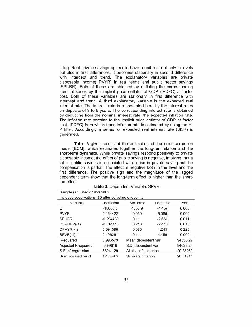
a lag. Real private savings appear to have a unit root not only in levelsbut also in first differences. It becomes stationary in second differencewith intercept and trend. The explanatory variables are privatedisposable income( PVYR) in real terms and public sector savings(SPUBR). Both of these are obtained by deflating the correspondingnominal series by the implicit price deflator of GDP (IPDFC) at factorcost. Both of these variables are stationary in first difference withintercept and trend. A third explanatory variable is the expected realinterest rate. The interest rate is represented here by the interest rateson deposits of 3 to 5 years. The corresponding interest rate is obtainedby deducting from the nominal interest rate, the expected inflation rate.The inflation rate pertains to the implicit price deflator of GDP at factorcost (IPDFC) from which trend inflation rate is estimated by using the H-P filter. Accordingly a series for expected real interest rate (SI3R) isgenerated.

Table 3 gives results of the estimation of the error correctionmodel [ECM], which estimates together the long-run relation and theshort-term dynamics. While private savings respond positively to privatedisposable income, the effect of public saving is negative, implying that afall in public savings is associated with a rise in private saving but thecompensation is partial. The effect is negative both in the level and thefirst difference. The positive sign and the magnitude of the laggeddependent term show that the long-term effect is higher than the short-run effect.

Table 3: Dependent Variable: SPVRSample (adjusted): 1953 2002

Included observations: 50 after adjusting endpoints

Variable Coefficient Std. error t-Statistic Prob.

C -18068.6 4053.9 -4.457 0.000

PVYR 0.154422 0.030 5.085 0.000

SPUBR -0.294430 0.111 -2.661 0.011

DSPUBR(-1) -0.514448 0.210 -2.448 0.018

DPVYR(-1) 0.094398 0.076 1.245 0.220

SPVR(-1) 0.496261 0.111 4.459 0.000

R-squared 0.996579 Mean dependent var 94558.22

Adjusted R-squared 0.99619 S.D. dependent var 94033.24

S.E. of regression 5804.129 Akaike info criterion 20.28269

Sum squared resid 1.48E+09 Schwarz criterion 20.51214

36

Table 3: Dependent Variable: SPVR (contd.)Sample (adjusted): 1953 2002

Included observations: 50 after adjusting endpoints

Variable Coefficient Std. error t-Statistic Prob.

Log likelihood -501.0673 F-statistic 2563.459

Durbin-Watson stat 1.73141 Prob (F-statistic) 0

Fiscal Deficit and Government Capital Expenditure

It has been argued in an earlier section that as interest ratesincrease relative to current revenues of the government, a process ofadjustment starts in government expenditure. This may lead to areduction in public investment, particularly, government investmentrelative to GDP. We look at the relationship between government capitalexpenditure, interest payments and revenue receipts with reference tothe combined account of central and state governments. These areconverted into real terms by deflating with the GDP deflator. All the threeseries are stationary in first difference. Table 4 gives the estimatedrelationship within the ECM framework. It is seen that while interestpayments in real terms affect negatively the real government capitalexpenditure, revenue receipts in real terms have a positive impact.

Table 4: Dependent Variable: RCMCEMethod: Least squares

Sample (adjusted): 1953 2002

Included observations: 50 after adjusting endpoints

Variable Coefficient Std. error t-Statistic Prob.

C 824.1816 1008.755 0.817028 0.4182

RCMIP -0.452654 0.110548 -4.094651 0.0002

RCMRR 0.237316 0.053105 4.468815 0.0001

DRCMRR(-1) -0.103212 0.09703 -1.063706 0.2931

RCMCE(-1) 0.545986 0.096808 5.639866 0

R-squared 0.951796 Mean dependent var 25509.16

Adjusted R-squared 0.947511 S.D. dependent var 13173.31

S.E. of regression 3018.071 Akaike info criterion 18.95726

Sum squared resid 4.10E+08 Schwarz criterion 19.14847

Log likelihood -468.9316 F-statistic 222.1319

Durbin-Watson stat 1.941086 Prob(F-statistic) 0

37

VI. Growth in Combined Debt of Centreand States: A Historical Perspective

The decision as to the appropriate level of fiscal deficit in thecurrent period has to take into account the levels of the accumulateddebt relative to GDP, particularly in view of the impact it has on interestliabilities. In an earlier contribution, we had looked at the experience ofdebt accumulation in respect of central debt-relative to GDP [Rangarajanand Srivastava, 2003]. In this paper, we look at the growth of thecombined debt-GDP ratio and examine the relative contribution ofcumulated primary deficits and the cumulated effect of the excess ofgrowth rate over interest rate over the period 1951-52 to 2001-02.Interest rate in this discussion refers to the effective interest rate of thecentral and state governments, calculated as the ratio of interestpayments in a year to the outstanding liabilities at the beginning of theyear. Throughout the forty-five year stretch from 1955-56 to 1999-00,the growth rate was in excess of the interest rate. Since 2000-01, forthree consecutive years, the growth rate has been less than the interestrate both in real and nominal terms. During the nineties, even when theGDP growth rate remained in excess of the interest rate, the gapbetween the two has been narrowing.

The standard specification of the equation describing debtdynamics with discrete time periods is given by equation (1) [bt = pt + bt-1

{(1+it)/ (1+gt)}]. As discussed in Rangarajan and Srivastava (2003),writing zt = bt - bt-1, equation (1) can also be written as

zt = pt - bt-1 [(gt –it) (1+gt)-1]

or pt = zt + bt-1 [(gt –it) (1+gt)-1] (21)

Summing up over any two benchmark years 1 and T, we have

Σ pt = Σ zt + Σ bt-1 [(gt –it) (1+gt)-1] (t=1,…, T) (22)

The term

A1= Σ zt /Σ pt (t=1,…T) (23)

38

shows the extent to which the cumulated primary deficits translate intoaccumulation of debt. On the other hand, the term

A2=Σ bt-1 [(gt –it )(1+gt )-1] /Σ pt (t=1,…T) (24)

shows the extent to which the impact of cumulated primary deficits isabsorbed by the excess of growth over interest rate. For the purpose ofthe historical review, debt includes external debt evaluated at historicalexchange rates and state debt does not include reserve funds anddeposits.

According to available information, the combined debt-GDP ratioof the central and state governments at the end of 1950-51 was 29.6percent. During 1951-52 to 1959-60 a little less than 13 percentagepoints were added to the debt-GDP ratio. An additional accretion ofabout 4 percentage points took place in the sixties. In the seventies,there was hardly any change in the debt-GDP ratio. It was in the eightiesand nineties (up to 2002-03) that there was an increase respectively of14.7 percentage points for each period in the debt-GDP ratio. Table 5and chart 3 show the relative effects of the cumulated primary deficitsand the factor reflecting the effect of growth-interest rate differential inthe process of accumulation of combined debt of the central and stategovernments since 1951-52. The Indian experience shows that asignificant part of the pressure of primary deficit could be absorbed bythe excess of growth over interest rates. In particular, it was able toabsorb nearly 72 percent of the cumulated primary deficits. Had thiscushion not been available, cumulated primary deficits through 1951-52to 2002-03 would have added about 169 percentage points to thecombined debt to GDP ratio.

39

Chart 3: Growth of State Debt Relative to GDP: Relative Roles ofCumulated Primary Deficits and Excess of Growth Over

Interest Rates

Key:Cum p: Cumulated primary deficit to GDP ratioCum b: Cumulated debt to GDP ratioCum w (g-i): Cumulated effect of weighted excess of growth over interestrate

The decade-wise picture indicates that in the fifties, 33.5 percentof the impact of cumulative primary deficit was absorbed by the growth-interest rate differential. The remaining 66.4 percent of the cumulatedprimary deficit of 19.4 percentage points resulted in an increase in thedebt-GDP ratio of 12.9 percentage points. In the sixties, the pressureput by the cumulated primary deficit was relatively larger (32.2percentage points). However, 88 percent of this was absorbed by thedifferential of growth over interest rate, resulting in only a small increaseof 3.9 percentage points in the debt-GDP ratio. During the seventies,

40

nearly hundred percent of the impact of cumulated primary deficit wasabsorbed by the growth/ interest rate differential leading to a negligibleincrease in the debt-GDP ratio. In the eighties and the nineties (up to2002-03), about 72 and 62 percent respectively of the pressure ofcumulated primary deficit could be absorbed by the (g-i) differential.Chart 3 also shows how the accumulated primary deficit was the mostpersistent factor in causing the debt-GDP ratio to rise and how thegrowth-interest differential was able to absorb a significant portion of it inseveral stretches of time.

Table 5: Decadewise Decomposition of Debt Accumulation Relative to GDP

Cumulated changes in Relative impact of

cumulated primary deficitIncrease indebt-GDP

ratio

Absorptionby growth-

interestdifferential

Debt-GDPratio

Primarydef-GDP

ratio

Growth &interest

ratedifferential

D/p W(g-i)/p

1951-52 to 1959-60 12.89 19.39 6.50 66.47 33.53

1960-61 to 1969-70 3.87 32.18 28.31 12.03 87.97

1970-71 to 1979-80 0.07 26.18 26.12 0.25 99.75

1980-81 to 1989-90 14.71 52.09 37.38 28.24 71.76

1990-91 to 2002-03 14.67 39.09 24.42 37.53 62.47

1951-52 to 2002-03 46.21 168.94 122.73 27.82 72.18

Memo:

1996-97 to 2002-03 19.55 19.77 0.22 101.14 1.13

Debt-GDP Ratio at the end of--

1950-51 29.6

2002-03 75.8 Source: (Basic Data): Indian Public Finance Statistics, Ministry of Finance, Government ofIndia, and National Income Accounts, CSO.

However, for three consecutive years, viz., 2000-01, 2001-02,and 2002-03, the nominal growth rate fell below the effective interestrate. In these years, instead of absorbing the impact of primary deficits,the growth-interest differential, being negative, worked in the reverse byadding to the debt-GDP ratio. Further, since this effect depends on theprevious year’s debt-GDP ratio, its impact became progressively largerfor the same shortfall in the growth rate relative to the interest rate. At the

41

end of 2002-03, the combined debt-GDP ratio stood at 76 percent whenexternal debt is evaluated at historical exchange rates and, for thestates, reserve funds and deposits are not included. If these adjustmentsare made, the combined debt-GDP ratio at the end of 2002-23 isestimated to be about 85 percent of GDP.

VII. Medium and Short Term Fiscal Policy Stance

The management of fiscal deficit needs to distinguish betweenthe long term or trend growth after adjusting for the cyclical component ofgrowth and correspondingly between structural or cyclically neutral deficitand transitory deficit. The structural deficit must be determined within asustainability framework aiming at maximising trend growth rate. Theshort-term component of fiscal deficit should be used to minimise theimpact of cyclical changes while keeping the economy along its longterm growth path. The use of discretionary expenditure to stimulate theeconomy when it is below potential output and contain inflationarypressure when prices are above trend levels is meant to serve theobjective of macroeconomic stabilisation. The neo-classical analysisargues about the deleterious effect of high permanent deficits on savingsand suggests stabilising fluctuations around the equilibrium path withhigh rather than low level of national savings.

In the Maastricht Treaty (MT) norms read with the Pact onGrowth and Stability (PSG), it is provided for the member countries thatunder normal circumstances the structural balance should be zero and,when facing a slow-down, the net budget deficit could be up to amaximum of 3 percent of GDP5. On a long-term basis the debt-GDP ratioshould not be allowed to exceed 60 percent of GDP. It is only under anexceptional down turn or recession that the budget deficit may beallowed to exceed the 3 percent reference value6.

Measuring Structural and Cyclical Components of Deficit

Several methods have been used in the literature for estimatingstructural deficit. Considering actual fiscal deficits as the sum ofstructural and cyclical components, if one of the two components is

42

estimated, the other can be derived as a residual. There are three mainmethods that have been used in the literature: (a) constant elasticitiesmethod, where the cyclical component is estimates first based onestimated of revenue and expenditure elasticities with respect to income;(b) smoothed-ratio approach where the structural fiscal deficit isestimated first by smoothening the revenue and expenditure ratios toGDP; and (c) structural time series approach where time-varyingelasticities are used and the cyclical component is estimated first. Thereare some difficulties with each of these approaches. The more traditionalapproach of constant elasticities used by OECD, among others, involvesa three-step procedure. First, the output gap is calculated by taking thedifference between potential output and actual output; secondly,response of revenue and expenditure categories to changes in theoutput gap are calculated by estimating the relevant elasticities,providing an estimate of the cyclical component of deficit; and finally, thestructural deficit is calculated as a residual. As shown by Barrel et.al.,(1994), and Bradner, Diebalk, and Schuberth (1998), estimates ofstructural balances are highly sensitive to the method of estimating trendoutput and uncertainty surrounding the output-elasticities of expenditureand revenue categories. The structural time series approach, assuggested by Jaeger (1990), also has some problems. In particular, thevariances of the parameters are not well defined. It has been shown byHarvey (1989) that in such models, the exogenous variables must bebounded from above and non-stochastic. Url (1997) has pointed out thatnominal potential output cannot be regarded as bounded from above.The smoothed-ratio approach, suggested by Cano and Kanutin (1996)provides a direct and simpler method of calculating the structural deficit.In this approach, revenues and expenditures, expressed as ratios toGDP, are decomposed into a structural and residual component by usinga Hodrick – Prescott (H-P) filter7.

Let rs and es be the trend ratios of revenues and expendituresrelative to GDP (these can be disaggregated categories also), and rc andec be corresponding cyclical components. Then the structural deficit toGDP ratio is derived directly as

fs= es-rs (25)

The cyclical deficit fc is obtained as a residual. Bradner, Diebalk,and Schuberth (1998) argue that this method has several advantages.The H-P filter is relatively judgment free since only one parameter,

43

namely the length of the business cycle, has to be fixed. As a directmethod, it is able to exclude transitory non-cyclical events. The linearityof the H-P filter also facilitates using a disaggregated approach since thedisaggregated structural components add to 1. This method is also notvery demanding in terms of data requirements. One disadvantagehowever, is that it cannot capture the impact of fiscal policy changes ifthese are located at the end-points of the sample.

Trends in Structural and Cyclical Deficits

In this analysis, a distinction is made between structural fiscaldeficit and structural primary deficit by calculating the trend ratios ofprimary expenditure (pes) and interest payments relative to GDP ips

separately. Thus,

fs= (pe) s-rs+(ip) s and fc= f-fs (26)

Thus, f = ps + (ip)s + fc where ps = (pe)s – rs (27)

The fiscal deficit to GDP ratio thus has three components:primary structural deficit, structural interest payments relative to GDP,and cyclical fiscal deficit. Table 6 shows the structural and actual fiscaldeficits since 1990-91. Clearly, structural fiscal deficits account for alarge part of actual fiscal deficit in the nineties. The correspondingestimates for the years since 1951-52 are given in table A2. Structuralinterest payments to GDP ratio has increased continuously from 4.3percent in 1990-91 to 5.9 percent in 2001-02, amounting to an increaseof 2.6 percentage points. Structural primary deficit can be seen to havefallen from the peak of 4.14 percent in 1990-91 to 2.75 percent in 1997-98, before it started rising again. Although both factors have contributedto structural fiscal deficit, the impact of structural interest payments hasbeen larger in the nineties and also more persistent.

44

Table 6: Combined Central and State Finances: Structural and Cyclical Deficits Relative to GDP

(percent to GDP)

Actualfiscaldeficit

Struc-turalfiscaldeficit

Cycli-calfiscaldeficit

Struc-turalprim-arydeficit

Debt-stabili-singprimarydeficit

Actualinter-estpay-ments

Struct-uralinterestpaym-ents

1990-91 9.383 8.433 0.950 4.144 4.4757 4.397 4.288

1991-92 7.162 8.302 -1.140 3.822 3.2284 4.746 4.480

1992-93 7.240 8.171 -0.931 3.516 2.9542 4.792 4.656

1993-94 9.824 8.059 1.765 3.243 2.8343 4.953 4.816

1994-95 6.945 7.975 -1.030 3.012 4.3319 5.128 4.963

1995-96 6.778 7.947 -1.169 2.846 3.8711 4.962 5.101

1996-97 6.081 7.993 -1.912 2.757 2.5044 5.111 5.236

1997-98 7.660 8.118 -0.459 2.748 0.5467 5.159 5.370

1998-99 8.227 8.309 -0.083 2.801 1.9892 5.318 5.508

1999-00 9.002 8.548 0.453 2.899 0.3002 5.682 5.650

2000-01 8.792 8.816 -0.024 3.022 -1.1835 5.727 5.794

2001-02 10.557 9.099 1.458 3.159 -0.4902 6.098 5.939Source (basic data): Indian Public Finance Statistics and National Income Accounts.

Structural Primary Gap

The structural ‘primary gap’ is defined as the difference betweenactual structural primary deficit and the debt-stabilising primary deficit(ps) defined as {bt-1*(1+gt)/(gt-it)}. Table 6 also shows that the primarydeficit has been higher than the ‘debt-stabilising’ primary deficit, in mostof the years in the nineties except 1990-91, 1994-95, and 1995-96. Thestructural primary balance has been used in the literature to assess themedium-term fiscal stance. The large values of the structural primarybalance since the late nineties clearly indicate that the current medium-term fiscal stance is not sustainable.

The profile of structural and debt-stabilising primary deficit iscompared in chart 4 since 1951-52. The structural primary deficit isshown by the bolder line. There are long stretches towards the end of theeighties and the latter part of the nineties that the structural primary

45

deficit has been much higher than the debt-stabilising primary deficit.These are the episodes in time where large accretion of debt relative toGDP took place. This led to larger structural interest payments relative toGDP. Together, structural primary deficit and structural interestpayments have caused structural fiscal deficits to be large.

Chart 4: Comparison of Structural and Debt-Stabilizing PrimaryDeficit

In view of the large structural fiscal deficit, the role that cyclical

Chart 4: Comparison of Structural and Debt-Stablising Primary Deficit

In view of the large structural fiscal deficit, the role that cyclicaldeficit can play has become extremely limited in periods of recession.Table A3 shows estimates of cyclical deficit against the differencebetween actual growth rate and trend growth rate. It is expected that asuitable short-term fiscal stance would show opposite signs betweencyclical deficit and departures of actual growth from trend growth, that is,when actual growth is below trend, the cyclical deficit should be positiveand vice versa. It would be seen that throughout the period from 1965-66to 1987-88, the short-term stance was in the correct direction. It is in theperiod since 1988-89 that the short-term stance has not been robustexcept in the mid-nineties.

46

Policy Options

In considering the policy options for India at the current juncture,it may be noted that the debt-GDP ratio, according to availableinformation, is estimated to be in excess of 80 percent of GDP at the endof 2004-05. This includes reserve funds and deposits for both the centreand states but external debt is evaluated at historical exchange rates.Also, liabilities of the market stabilisation fund are not included againstwhich an equivalent asset in the form of cash reserves is held with theRBI. Ruling out any further increase in the debt-GDP as undesirable, thepolicy option is whether to stabilise the debt-GDP ratio at its present levelor bring it down before stabilising. From the viewpoint of a suitablemedium-term fiscal policy stance, a combination of high fiscal deficit,high debt, and high-interest payments relative to-GDP will negativelyimpact on the trend-growth rate by keeping the saving-GDP ratio belowits potential. By reducing the debt-GDP ratio, interest payments relativeto GDP will also be reduced such that, in combination with feasible levelsof revenue receipts relative to GDP, government will be able to balanceits revenue account and eliminate dissaving. Such a fiscal stance wouldfacilitate achieving a higher level of growth rate on a sustained basis.This calls for a period of adjustment during which fiscal deficit is loweredeach year from the previous year’s level such that, in each successiveyear, the debt-GDP ratio falls. This adjustment phase may continue untilrevenue deficit is eliminated. Thereafter, a stabilisation phase canemerge when the fiscal deficit may remain constant at a level leadingeventually also to debt-stabilisation.

The FRBMA enacted by the central government, read with itsrules and subsequent amendment, specifies the target for achieving afiscal deficit to GDP ratio of 3 percent by 2008-09. The FRBMA, as itstands at present, is incomplete in two respects. First, it does not definea debt-GDP ratio that would be required for keeping the economy on itspotential growth path, and secondly, it does not define suitable limits ofdeparture from the medium-term stance to cope with cyclical fluctuations.The prescription under the FRBMA can be evaluated in relation to theMaastricht Treaty norms read with the Growth and Stability Pact. In theEuropean context, countries are supposed to maintain balance (zerofiscal deficit) under normal circumstances and up to 3 percent fiscaldeficit, when faced with a downturn. Undoubtedly, the higher growth ratein India will allow a higher level of fiscal deficit relative to GDP to bemaintained. A combined fiscal deficit of 6 percent of GDP for the

47

government sector would be consistent with the available supply of fundsin the form of financial savings of the household sector of the order ofabout 10-11 percent of GDP and feasible levels of current account deficitof about 1.5 to 2 percent of GDP. This order of supply of funds would beadequate for meeting the demand for these funds from the privatecorporate sector to an extent of about 4-5 percent of GDP, demand fromthe government sector (administrative departments and departmentalenterprises) of 6 percent of GDP (fiscal deficit) and that from the non-departmental public enterprises of about 1.5 to 2 percent of GDP. Thus,a combined fiscal deficit of 6 percent of GDP is consistent with theexisting ratio of the savings of the household sector in financial assetsrelative to GDP and prudent levels of current account deficit, and thedemand on these by the private corporate sector and non-departmentalpublic enterprises.

The FRBMA of the central government has indicated the need tocontain the fiscal deficit of the centre to 3 percent of GDP by 2008-09. Indetermining a limit for the states considered together, it might berecognised that the states have a higher share in the combined revenuereceipts after transfers, and therefore, in the context of sustainability,they may be allowed a higher limit of fiscal deficit relative to GDP. Butthe states also face a higher interest rate on average. If these two factorsroughly neutralise each other, allowing a target limit of fiscal deficitrelative to GDP for the states similar to that for the centre, it would resultin a ratio of interest payments to revenue receipts for the states similar tothat for the centre8. Thus, fiscal deficit may be stabilised at 6 percent ofGDP on the combined account of the central and state governments with3 percent each on their separate accounts, assuming that these levels offiscal deficits relate to the ‘own’ requirements of the two levels ofgovernment. This should be considered as the relevant target over acycle. The Twelfth Finance Commission in the suggested programme forrestructuring public finances has recommended the target of reaching acombined fiscal deficit of 6 percent of GDP by 2008-09. Among importantobservers of the fiscal scene in India, Chelliah (2001, 2004) has arguedfor this level of combined fiscal deficit. In a recent analysis of debtsustainability, Ram Mohan, Dholakia, and Karan (2005), while dealingwith central debt, highlight a number of measurement issues. In theiradjustment programme, two scenarios are drawn with alternativeassumptions. In both cases, the central fiscal deficit to GDP ratio isbrought down to 3.9 percent by 2009-10. This is under the assumption ofthe system of on-lending from the central to state governments being

48

continued. About 0.8 percentage points of central fiscal deficit may onlybe for on-lending to the states. Thus, for central fiscal deficit,representing borrowing only for ‘own’ needs, the target level afteradjustment that is considered feasible in their analysis does not appearto be much different from the one suggested here, although there aredifferences in the initial levels.

As already mentioned, before the stabilisation phase is reached,

the Indian economy will have to pass through an adjustment phase.During this phase, the debt-GDP ratio will have to fall. This can be doneby reducing the fiscal deficit to GDP ratio each year to a level lower thanthat, which will stabilise the debt-GDP ratio at the previous year’s level.For example, if the previous year’s debt-GDP ratio is 80 percent, and thenominal growth rate is 12 percent, a fiscal deficit to GDP ratio of about8.57 percent would leave it unchanged at 80 percent at the end of thecurrent year. A fiscal deficit that is below this level would lead to areduction in the debt-GDP ratio. The period of the adjustment phase willbe shorter, the larger the extent by which the actual fiscal deficit relativeto GDP is lower than the debt-stabilising level, and the faster theimprovement in the revenue to GDP ratio on the combined account ofcentral and state governments. Once the adjustment phase is over, andthe combined fiscal deficit of the centre and the states remains fixed at 6percent, the debt-GDP ratio would still keep falling and eventuallystabilise at 56 percent of GDP9. This is under the assumption that thenominal growth rate would be 12 percent. At that stage, the interestpayments to revenue receipts ratio will stabilise at 17 percent10 . Thisratio would be most desirable as it would permit a larger primary revenueexpenditure to be incurred on the social sectors. In fact, this will behappening as the ratio of interest payments to revenue receipts begins tofall from its present level of around 34 percent. The decomposition of thisoverall interest payment to revenue receipts ratio between the centre andthe states will depend on their revenue receipts to GDP ratios and theirrespective average interest rates. Maintaining balance on revenueaccount will be facilitated as interest payment to GDP ratio falls. Underthese circumstances, the government can maintain a capital expenditureto GDP ratio reasonably above 6 percent with some positive non-debtcapital receipts. In the medium term, a strategy of fiscal correctionbroadly on these lines would support growth on a sustained basis asgovernment dissavings are reduced and government capital expenditure,focused on infrastructure, is increased and kept above the level of 6

49

percent of GDP. The behaviour of the debt-GDP ratio under theproposed reform scenario is given in chart 5 and appendix table A4.

Chart 5: Debt and Fiscal Deficit to GDP Ratios under the Reform Scenario

Note: Debt-GDP ratio (b) is shown on the left hand vertical axis and fiscal deficitto GDP ratio (fa) is shown on the right hand vertical axis with a different scale.

An argument is sometimes advanced that in the currenteconomic scenario, higher fiscal deficits should be used foraccommodating higher expenditure on infrastructure and social sectors.While an increase in expenditures in some of these areas may bedesirable and even necessary, they ought to be undertaken in such away that there is no increase in primary deficit and debt-GDP ratio.Expenditure prioritisation is thus requisite under such a situation. In fact,as a result of expanding expenditures, government dissaving increases,a sustained increase in the growth rate cannot emerge. With high levelsof revenue deficit, increased levels of expenditures on infrastructure andsocial sectors cannot also be sustained. As demand for funds from theprivate corporate sector increases, it cannot be assumed that the cost offunds will remain benign, if government dis-savings do not come down.An appropriate medium term strategy is to control fiscal deficit, reducedebt-GDP ratio so that interest payments relative to revenue receipts can

0.0

10.0

20.0

30.0

40.0

50.0

60.0

70.0

80.0

90.0

2004

-05

2006

-07

2008

-09

2010

-11

2012

-13

2014

-15

2016

-17

2018

-19

2020

-21

2022

-23

2024

-25

2026

-27

2028

-29

2030

-31

2032

-33

2034

-35

2036

-37

0.0

1.0

2.0

3.0

4.0

5.0

6.0

7.0

8.0

9.0

10.0

b fa

50

be reduced and government dissavings can be eliminated. This willaugment the overall saving rate. With stable costs of borrowing, overallinvestment will increase to sustain a growth rate of 7 percent and above.With the ratio of revenue deficit to GDP coming down progressively tozero, the entire amount of borrowing supplemented by non-debt capitalreceipts can be used for capital investment by the government. The righttime for the adjustment phase is at present when the economy is on theupswing.

VIII. Concluding Observations

This paper has looked at the impact of fiscal deficits on saving,investment, and growth in the light of the theoretical literature on thesubject in the context of the fiscal deficit and debt on the combinedaccounts of the central and state governments. Revenue deficits amountto reduction in government savings, which may not be fully offset by acorresponding rise in the private savings, leading to a fall in the overallsaving rate. The impact of fiscal deficit on investment arises both from itsimpact on private investment and government investment. The adverseeffects on private investment occur if fiscal deficits put pressure oninterest rates, and if private investment is sensitive to the interest rate.The effect on government capital expenditure is through committedinterest payments, which rise if the debt-GDP ratio rises and/or interestrate rises. In the context of debt accumulation in India, the main findingsare summarised below.

• Fiscal deficit and government debt in India, have received growingattention of analysts and policymakers, particularly since thenineties, when in most years the combined fiscal deficit was higherthan 9 percent of GDP. The concerns have become more serious inrecent years when there has been an explosive rise in the debt-GDPratio in spite of the fact that the nominal interest rates have fallen.This is because, during 2000-03, nominal growth rates fell evenmore. With growth rate being less than the effective interest rate, thedebt-GDP ratio increased both because of cumulated primary deficitsand excess of interest rate over growth rate during 2000-01 to 2002-03.

51

• Even if fiscal deficits may appear to be sustainable according tosome studies, the critical issue relates to determining appropriatelevels of debt and deficit relative to GDP on which these should bestabilised. This can be done by developing rules with given growthand interest rates and initial debt levels. However, since fiscaldeficits and debt affect growth and interest rates, answers need to bederived using information on their impact on savings and investment,which ultimately determine the growth rate. The interest rates arealso affected by the fiscal deficit and monetary policy, but there mayalso be exogenous influences, particularly international interest ratesand inflow of foreign capital.

• When fiscal deficits are high in magnitude relative to GDP andlargely structural in nature, government’s ability to mount counter-cyclical interventions could be compromised, particularly whengrowth is below trend levels and intervention is needed. This wasclearly experienced in the late nineties and the early part of the newdecade.

• In India, the household sector saves more than it invests, and theexcess becomes available in the form of financial savings of thissector to the private corporate sector and the government sector fortheir investment requirements that are not financed by their ownsavings. Although government dissavings increased since the latenineties, the pressure on interest rates was not witnessed becauseof a fall in investment demand by the private corporate sector. Thismay prove to be temporary.

• The overall growth rate depends on the overall savings rate andinvestment rate. There is reason to believe that when governmentsaving falls, private saving rate increases as wealth held in theprivate sector in the form of government bonds increases. Thiscompensatory rise in the private sector saving rate has been partial.On the investment side, government’s own investment demand alsofell as its debt-GDP ratio and the ratio of interest payments torevenue receipts rose. Empirical tests indicate that governmentcapital expenditures do respond negatively to the interest paymentsand positively to revenue receipts. If interest payments rise fasterthan revenue receipts, government capital expenditure falls. Privateinvestment responds negatively to a rise in expected interest rates.In the nineties and beyond, government capital expenditures relativeto GDP fell not only because interest payments relative to GDPincreased but also because ratio of revenue receipts to GDP fell.

52

• The FRBMA has certain positive features. It is incomplete in tworespects. One, it does not indicate a suitable level of debt-GDP ratioalong with the specified fiscal deficit target, and secondly, it does notprovide for a suitable strategy for coping with short-term fluctuations.

• It is important that centre’s FRBMA is supplemented by state levelfiscal responsibility legislations because, taken together, states’borrowing and debt contribute significantly to the overall fiscal deficitand debt relative to GDP and have significant macro implications.

• To achieve and sustain growth at high levels, it is required that theoverall savings ratio is increased leading to a rise in the investmentratio, and revenue and fiscal deficits should be so managed as toserve this purpose. In the context of the present policy options, thereis a need to bring down the debt-GDP ratio from its present level,which is in excess of 80 percent of GDP. The process of adjustmentcan be considered in two phases: adjustment phase and stabilisationphase. In the adjustment phase, fiscal deficit will have to be reducedin each successive year to a level, which is less than the level offiscal deficit relative to GDP that will stabilise the debt-GDP ratio atits previous year’s level. This phase should be continued until therevenue deficit is eliminated. In the second phase, the fiscal deficitcould be stabilised at 6 percent of GDP. In this phase, the debt-GDPratio would fall for some more years and eventually stabilise at 56percent. At this level of debt-GDP ratio, it is estimated that theinterest payment to revenue receipts ratio, under given assumptions,would fall to 17 percent. As the ratio of interest payments to revenuereceipts begins to fall, it will enable a progressively larger amount ofprimary revenue expenditure to be incurred on the social sectors.

54

References

Abel, Andrew et.al. “Assessing Dynamic Efficiency: Theory andEvidence”, Review of Economic Studies, Vol. 56, 1989; 1-20.

Barro, Robert J. “Are Government Bonds Net Wealth?”, Journal ofPolitical Economy, 82, November/December 1974;1095-1117.

Barro, Robert “Reply to Feldstein and Buchanan”, Journal of PoliticalEconomy, 84(2), 1976; 343-49.

------------------. “On the Determination of the Public Debt,” Journal ofPolitical Economy, 87 October 1979; 940-971.

-----------------. “Government Spending, Interest Rates, Prices, and BudgetDeficits in the United Kingdom, 1701-1918,” Journal of MonetaryEconomics, 20 September 1987; 221-247.

----------------. “The Ricardian Approach to Budget Deficit”, Journal ofEconomic Perspectives, 3(2), 1989; 37-54.

Barrel, R. et.al. The Cyclical Adjustment of Budget Balances, ReportSeries No.8, National Institute of Economic and Social Research (1994).

Barsky, Robert et.al. “Ricardian Consumers with KeynesianPropensities”, American Economic Review, 76 September 1986; 676-691.

Bernheim, B. Douglas and Kyle Bagwell. “Is Everything Neutral?”Journal of Political Economy, 96, April; 308-338.

Bernheim, Douglas B. “A Neoclassical Perspective on Budget Deficits”,Journal of Economic Perspectives, 3(2), 1989; 55-72.

Bradner, P., L.Diebalek, and H. Schuberth. “Structural Budget Deficitsand Sustainability of Fiscal Positions in the European Union”, WorkingPaper No. 26, Oesterreichische National Bank (1998).

55

Buchanan, James M., Richard A. Musgrave 1999. Public Finance andPublic Choice: Two Contrasting Visions of the State. Cambridge,Massachusetts: MIT Press; 272.

Buiter, W.H. “Guide to Public Sector Deficit and Debt” Economic Policy,November, 1985;13-79.

----------------. “Some Thoughts on the Role of Fiscal Policy in Stabilisationand Structural Adjustment in Developing Countries”, Working Paper No.2603, NBER (May 1988).

Buiter, Willem H. and Urjit R Patel. ”Debt, Deficits and Inflation: AnApplication to the Public Finances of India”, Journal of Public Economics,47, March 1992; 172-305.

Cano, L., and A. Kanutin. “Estimation of Structural Deficits in EUCountries”, mimeo, London School of Economics (1996).

Chakraborty Lekha S. “Fiscal Deficit and Rate of Interest: AnEconometric Analysis of the Deregulated Financial Regime”, Economicand Political Weekly, 37(19), May 11, 2002.

Chelliah, R. J. 1996. “The Meaning and Significance of the FiscalDeficit”, in Towards Sustainable Growth: Essays in Fiscal and FinancialState Reforms in India, Delhi: Oxford University Press.

----------------------. 2001.“The Nature of the Fiscal Crisis in IndianFederation and Calibrating Fiscal Policy”, Money and Finance, ICRABulletin, 2(4-5).

----------------------. “Implementing FRBM Act, 2003: Evaluating KelkarTask Force Report”, Economic and Political Weekly, September, 2004.

Domar, E., “The ‘Burden’ of Public Debt and National Income”, AmericanEconomic Review, 34, 1944.

Eisner, Robert and Paul J Pieper. “A New View of the Federal Debt andBudget Deficit” American Economic Review, 74, March 1984;11-29.

Eisner, Robert. “Budget Deficits: Rhetoric and Reality”, Journal ofEconomic Perspectives, 3(2), Spring 1989; 73-93.

56

Engle, R.F. and C.W.J. Granger. “Cointegration and Error Correction:Representation, Estimation and Testing”, Econometrica, 55,1987; 251-276.

Feldstein, Martin S. “Perceived Wealth in Bonds and Social Security: AComment,” Journal of Political Economy, 84, April 1976;331-336.

Gale William G. and Orszag Peter R. “The Economic Effects of LongTerm Fiscal Discipline,” Urban-Brookings Tax Policy Center DiscussionPaper, December 17, 2002.

Goyal, Rajan, “Does Higher Fiscal Deficit Lead to Rise in Interest Rates?An Empirical Investigation”, Economic and Political Weekly, 39(21) May,2004; 2128-2133.

Gramlich, Edward M. “Budget Deficits and National Saving: ArePoliticians Exogenous”, Journal of Economic Perspectives, 3(2), 1989;23-35.

Harvey, A. 1989. Forecasting, Structural Time Series Models and theKalman Filter. Cambridge: Cambridge University Press.

Hsiao, C. “Cointegration and Dynamic Simultaneous Equation Model,”Econometrica, 65(3), May 1997;647-70.

------------. “Identification and Dichotomization of Long- and Short- RunRelations of Cointegrated Vector Autoregressive Models, EconometricTheory, 17, 2001;889-912.

Hodrick, R. and Prescott, E. “Post-War U.S. Business Cycles: AnEmpirical Investigation”, Discussion Paper No. 451, Carnegie-MellonUniversity, Pittsburgh (1981).

Inman, Robert P. “Do Balanced Budget Rules Work? US Experience andPossible Lessons for the EMU,” Working Paper 5838, National Bureau ofEconomic Research, Cambridge, MA 02138 (November, 1996).

Jaeger, A. “The Measurement and Interpretation of Structural BudgetBalances”, Empirica, 2(17), 1990.

57

Jha, R. and A. Sharma. “Structural Breaks, Unit Roots, andCointegration: A Further Test of the Sustainability of the Indian FiscalDeficit,” Public Finance Review, 32, 2004;220-231.

Johansen, S. “Estimation and Hypothesis Testing of CointegratedVectors in Gaussian Vector Autoregressive Models,” Econometrica, 59,1991;1555-1580.

Johansen, S. and K. Juselius. “Identification of the Long-run and ShortRun Structure: An Application to the ISLM Model,” Journal ofEconometrics, 63, 1995;7-36.

Joshi Vijay and IMD Little, “Fiscal Policy”, in Macroeconomics andPolitical Economy:1964-1991. Washington, D.C: The World Bank.

Juselius, K. “Do Purchasing Power Parity and Uncovered Interest RateParity Hold in the Long Run? An Example of Likelihood Inference inMultivariate Time Series Model”, Journal of Econometrics, 69, 1995;211-240.

Kotlikoff, Laurence J. “Applying Generational Accounting to DevelopingCountries”, IED Discussion Paper Series, No 67, Institute for EconomicDevelopment, Boston University (December, 1995).

-------------------. “Intergenerational Transfers and Savings”, Journal ofEconomic Perspectives, 2, 1988;41-58.

Lahiri, A. and R. Kannan , “India’s Fiscal Deficits and Their Sustainabilityin Perspective” Paper presented at World Bank-NIPFP seminar onFiscal Policies for Growth, New Delhi (2001).

Moorthy, Vivek, B. Singh, and S. C. Dhal. “Bond Financing and DebtStability: Theoretical Issues and Empirical Analysis for India”,Development Research Group Study, 19, RBI, Mumbai (June, 2000).

Papadopoulos, A. and M. Sidiropoulos, “The Sustainability of FiscalDeficit in the European Union”, Advances in Economic Research, 5(3),1999;289-307.

Parker, K. “The Behaviour of Private Investment”, IMF Occasional PaperNo.134, IMF, Washington,D.C. (1995).

58

Patnaik, Prabhat. “Fiscal Deficits and Real Interest Rates”, Economicand Political Weekly, April 12-20, 2001.

Pinto, Brian and Farah Zahir, “Why Fiscal Adjustment Now?”, Economicand Political Weekly, 39, March 6, 2004.

Pradhan, B. K. D. K. Ratha and Atul Sarma. “Complementarily BetweenPublic and Private Investment in India”, Journal of DevelopmentEconomics, 33, 1990.

Rajaraman, Indira and Abhiroop Mukhopadhyay, 2000. “Sustainability ofPublic Domestic Debt in India”, in (ed.) D.K. Srivastava, “FiscalFederalism in India: Contemporary Challenges, Issues before theEleventh Finance Commission”. New Delhi: Har Anand Publications Pvt.Ltd.

Rajaraman, I. S. Bhide, and R.K. Pattnaik, “A Study of DebtSustainability at the State Level in India”, Reserve Bank of India. 2004(mimeo).

Rakshit, Mihir. “On Correcting Fiscal Imbalances in the Indian Economy:Some Perspectives”, Money and Finance, ICRA Bulletin, 2(2), 2000.

------------------. “Budget Deficit: Sustainability, Solvency, and Optimally” in(ed.) A. Bagchi, 2005. Readings in Public Finance. New Delhi: OxfordUniversity Press. Ram Mohan et.al., “Is India’s Central Debt Sustainable? Revisiting anOld Debate”, Economic and Political Weekly, March 5, 2005.

Rangarajan, C. Anupam Basu and Narendra Jadhav. “Dynamics ofInteraction between Government Deficit and Domestic Debt in India”,RBI Occasional Papers, September, 1989; also included in AmareshBagchi and Nicholas Stern (eds.) (1994) Tax Policy and Planning inDeveloping Countries. New Delhi: Oxford University Press.

Rangarajan, C. and D.K. Srivastava, “Dynamics of Debt Accumulation inIndia: Impact of Primary Deficit, Growth and Interest Rate, Economic andPolitical Weekly”, 38(46), November, 2003.

Reserve Bank of India, 2002. Report on Currency and Finance, 2000-01.

59

Reynolds, Patricia. “Fiscal Adjustment and Growth Prospects in India”, in(eds.) 2001, Tim Callen, Patricia Reynolds, and Christopher Towe Indiaat the Crossroads: Sustaining Growth and Reducing Poverty.Washington D.C: International Monetary Fund.

Seshan, A. “The Burden of Domestic Public Debt in India, RBIOccasional Papers, 8(1), 1987.

Shigehara Kumiharu. “Commentary: Long Term Tendencies in BudgetDeficits and Debt”, in Budget Deficits and Debt: Issues and Options,Proceedings of a Symposium Federal Reserve Bank of Kansas City,USA (August 31-September 2).

Sunderarajan, V. and Subhash Thakur. “Public Investment, Crowing Out,and Growth: A Dynamic Model Applied to India and Korea”, IMF StaffPapers, 27(4), 1980.

Url, Th. “How Serious is the Pact on Stability and Growth?”, WorkingPaper No. 92, Austrian Institute of Economic Research, (1997).

Vedder, R., L.Galloway, and C.Frenze. “Federal Tax Increases and theBudget Deficit, 1947-86: Some Empirical Evidence”, Joint EconomicCommittee Minority Staff Paper (1987).

Khatkhate, Deena. “On Fiscal Deficits and Real Interest Rates”Economic and Political Weekly, May 12, 2001.

Von Furstenberg, et.al., “Tax and Spend, or Spend and Tax”, Review ofEconomics and Statistics, 68, May 1986;179-188.

Yellen Janet L., “Symposium on the Budget Deficit”, Journal of EconomicPerspectives, 3(2), 1989;17-21.

60

Table A1: Savings and Investment Relative to GDP at Market Prices (percent to GDP)

Gross Domestic Savings Gross Domestic Capital FormationHousehold

sectorPrivate

corporatesector

Totalprivate

Publicsector

Total(2+3+4) Public

sectorPrivatesector

Total(12+13)

Adjustedtotal

(14+15)SH SPC SPVT SPUB S IPUB IPVT ISUM IADJ

1950-51 6.16 0.94 7.10 1.83 8.93 2.78 7.73 10.51 8.721951-52 5.52 1.29 6.80 2.52 9.32 3.04 7.81 10.85 11.051952-53 6.15 0.62 6.76 1.54 8.31 2.64 6.20 8.85 7.981953-54 5.81 0.80 6.60 1.27 7.87 2.76 4.63 7.38 7.761954-55 6.73 1.11 7.84 1.57 9.41 4.47 5.49 9.96 9.561955-56 9.62 1.23 10.85 1.75 12.60 4.80 7.72 12.52 12.961956-57 9.10 1.20 10.29 1.94 12.23 5.34 9.19 14.52 15.011957-58 7.47 0.91 8.38 1.99 10.37 6.43 8.24 14.68 13.911958-59 6.83 0.94 7.77 1.69 9.46 5.67 6.02 11.70 11.991959-60 8.30 1.18 9.48 1.67 11.15 5.95 7.47 13.42 12.631960-61 7.30 1.64 8.94 2.64 11.59 6.86 7.79 14.66 14.391961-62 7.04 1.76 8.80 2.89 11.69 6.52 8.44 14.96 13.591962-63 7.84 1.76 9.59 3.08 12.67 7.62 8.04 15.65 14.921963-64 7.20 1.75 8.95 3.34 12.29 7.71 7.76 15.47 14.251964-65 7.15 1.48 8.63 3.30 11.93 7.65 7.88 15.54 14.221965-66 9.40 1.46 10.87 3.12 13.99 8.25 8.08 16.33 16.151966-67 10.30 1.35 11.65 2.33 13.98 7.06 9.53 16.59 16.921967-68 8.76 1.12 9.88 2.01 11.88 6.59 8.64 15.23 14.171968-69 8.63 1.13 9.76 2.40 12.16 5.82 8.56 14.38 13.231969-70 10.39 1.28 11.67 2.61 14.28 5.52 9.82 15.34 14.841970-71 10.15 1.47 11.62 2.94 14.56 6.39 9.43 15.82 15.421971-72 10.67 1.57 12.24 2.82 15.06 6.98 9.95 16.93 16.031972-73 10.43 1.49 11.92 2.67 14.59 7.18 8.98 16.17 15.14

61

Table A1: Savings and Investment Relative to GDP at Market Prices (contd.) (percent to GDP)

Gross Domestic Savings Gross Domestic Capital FormationHousehold

sectorPrivate

corporatesector

Totalprivate

Publicsector

Total(2+3+4) Public

sectorPrivatesector

Total(12+13)

Adjustedtotal

(14+15)SH SPC SPVT SPUB S IPUB IPVT ISUM IADJ

1973-74 12.17 1.65 13.82 2.94 16.76 7.47 9.18 16.66 17.361974-75 10.43 1.89 12.32 3.66 15.98 7.43 10.89 18.32 16.821975-76 11.70 1.30 13.00 4.23 17.23 9.37 9.60 18.97 17.091976-77 13.20 1.32 14.52 4.88 19.40 9.83 9.27 19.10 17.941977-78 14.13 1.39 15.52 4.31 19.83 7.97 10.71 18.68 18.381978-79 15.45 1.50 16.95 4.55 21.50 9.23 11.48 20.71 21.611979-80 13.81 1.98 15.80 4.32 20.12 10.04 11.33 21.37 20.601980-81 13.82 1.63 15.45 3.43 18.88 8.42 10.27 18.69 20.331981-82 12.59 1.52 14.11 4.49 18.60 10.07 12.34 22.41 20.151982-83 12.33 1.58 13.91 4.34 18.26 10.70 10.97 21.66 19.621983-84 12.83 1.48 14.31 3.27 17.58 9.69 9.99 19.68 18.731984-85 14.28 1.65 15.93 2.83 18.76 10.43 11.17 21.60 20.101985-86 14.32 1.95 16.27 3.22 19.49 10.79 12.88 23.67 21.731986-87 14.48 1.71 16.20 2.75 18.94 11.17 12.03 23.20 20.991987-88 16.69 1.67 18.37 2.21 20.58 9.53 12.59 22.11 22.501988-89 16.76 2.01 18.77 2.08 20.85 9.52 14.17 23.69 23.771989-90 17.89 2.44 20.32 1.68 22.00 9.54 14.12 23.66 24.531990-91 19.33 2.67 21.99 1.10 23.10 9.34 14.73 24.07 26.301991-92 16.96 3.11 20.06 1.97 22.03 8.82 13.11 21.93 22.551992-93 17.51 2.67 20.18 1.59 21.77 8.55 15.24 23.79 23.611993-94 18.42 3.48 21.90 0.63 22.53 8.24 13.01 21.25 23.091994-95 19.68 3.48 23.17 1.66 24.83 8.71 14.67 23.38 26.001995-96 18.19 4.93 23.12 2.03 25.15 7.66 18.87 26.53 26.90

62

Table A1: Savings and Investment Relative to GDP at Market Prices (contd.) (percent to GDP)

Gross Domestic Savings Gross Domestic Capital FormationHousehold

sectorPrivate

corporatesector

Totalprivate

Publicsector

Total(2+3+4) Public

sectorPrivatesector

Total(12+13)

Adjustedtotal

(14+15)SH SPC SPVT SPUB S IPUB IPVT ISUM IADJ

1996-97 17.05 4.47 21.51 1.67 23.19 7.03 14.74 21.77 24.481997-98 17.63 4.17 21.80 1.33 23.13 6.61 15.96 22.57 24.601998-99 18.77 3.74 22.51 -0.99 21.52 6.58 14.80 21.38 22.571999-00 20.88 4.35 25.23 -1.04 24.20 6.94 16.72 23.66 25.332000-01 21.93 4.12 26.05 -2.31 23.74 6.29 16.33 22.62 24.352001-02 22.74 3.46 26.20 -2.75 23.45 5.83 16.48 22.31 23.132002-03 22.65 3.41 26.05 -1.85 24.20 5.68 17.15 22.83 23.28

Source: National Income Accounts, CSO.

Table A2: Combined Central and State Finances: Structural and Cyclical Deficits (percent to GDP)

Actualfiscal

deficit

Structuralfiscal

deficit

Cyclicalfiscal

deficit(1-2)

Structuralprimary

deficit (2-7)

Debt-stabilising

primarydeficit

Actualinterest

payments

Structuralinterest

payments

Structuralprimary

gap(4-5)

(1) (2) (3) (4) (5) (6) (7) (8)1951-52 1.121 0.850 0.271 0.160 1.1299 0.644 0.690 -0.9691952-53 0.639 1.371 -0.733 0.614 -1.283 0.724 0.757 1.8961953-54 0.701 1.896 -1.195 1.071 1.714 0.736 0.825 -0.6431954-55 2.582 2.418 0.164 1.527 -2.647 1.040 0.891 4.1751955-56 2.771 2.922 -0.151 1.968 -0.556 1.140 0.954 2.5241956-57 2.928 3.393 -0.465 2.379 4.626 0.957 1.014 -2.247

63

Table A2: Combined Central and State Finances: Structural and Cyclical Deficits (contd.) (percent to GDP)

Actualfiscal

deficit

Structuralfiscal

deficit

Cyclicalfiscal

deficit(1-2)

Structuralprimary

deficit (2-7)

Debt-stabilising

primarydeficit

Actualinterest

payments

Structuralinterest

payments

Structuralprimary

gap(4-5)

(1) (2) (3) (4) (5) (6) (7) (8)1957-58 4.913 3.813 1.099 2.741 -0.031 0.989 1.072 2.7721958-59 6.312 4.163 2.149 3.033 2.713 0.988 1.130 0.3201959-60 5.785 4.432 1.353 3.244 0.836 1.142 1.188 2.4081960-61 3.506 4.631 -1.125 3.387 2.425 1.270 1.245 0.9611961-62 2.928 4.786 -1.858 3.487 1.053 1.341 1.298 2.4351962-63 3.987 4.909 -0.923 3.562 1.534 1.467 1.348 2.0271963-64 4.862 4.997 -0.135 3.605 4.339 1.348 1.392 -0.7341964-65 5.723 5.035 0.689 3.604 4.783 1.350 1.431 -1.1801965-66 5.658 5.007 0.652 3.542 0.705 1.525 1.465 2.8371966-67 9.705 4.904 4.801 3.412 3.672 1.677 1.493 -0.2601967-68 4.529 4.726 -0.197 3.212 5.790 1.558 1.514 -2.5781968-69 3.251 4.517 -1.267 2.987 1.114 1.551 1.530 1.8741969-70 2.648 4.322 -1.674 2.779 2.894 1.530 1.543 -0.1151970-71 2.380 4.172 -1.792 2.617 1.337 1.635 1.555 1.2801971-72 6.816 4.081 2.734 2.514 1.346 1.700 1.567 1.1681972-73 4.126 4.047 0.079 2.463 3.006 1.602 1.583 -0.5421973-74 1.100 4.092 -2.992 2.485 7.195 1.532 1.607 -4.7101974-75 3.037 4.242 -1.205 2.599 4.841 1.508 1.643 -2.2421975-76 2.090 4.492 -2.403 2.798 1.258 1.394 1.694 1.5401976-77 7.361 4.824 2.537 3.061 0.762 1.948 1.763 2.2991977-78 7.118 5.198 1.921 3.348 3.206 1.723 1.849 0.1421978-79 3.312 5.596 -2.284 3.643 1.453 1.990 1.953 2.190

64

Table A2: Combined Central and State Finances: Structural and Cyclical Deficits (contd.) (percent to GDP)

Actualfiscal

deficit

Structuralfiscal

deficit

Cyclicalfiscal

deficit(1-2)

Structuralprimary

deficit (2-7)

Debt-stabilising

primarydeficit

Actualinterest

payments

Structuralinterest

payments

Structuralprimary

gap(4-5)

(1) (2) (3) (4) (5) (6) (7) (8)1979-80 6.086 6.023 0.062 3.949 1.713 2.212 2.075 2.2361980-81 7.372 6.459 0.912 4.246 5.342 2.065 2.214 -1.0961981-82 5.983 6.886 -0.903 4.514 4.611 2.228 2.372 -0.0971982-83 9.177 7.293 1.884 4.743 2.295 2.464 2.550 2.4481983-84 5.389 7.661 -2.272 4.916 4.581 2.531 2.745 0.3351984-85 8.551 7.991 0.560 5.035 2.189 2.925 2.956 2.8461985-86 8.995 8.261 0.734 5.082 2.895 3.144 3.179 2.1871986-87 10.123 8.452 1.671 5.045 2.385 3.443 3.407 2.6601987-88 9.010 8.556 0.454 4.918 3.514 3.666 3.637 1.4041988-89 9.089 8.578 0.510 4.715 5.790 3.901 3.863 -1.0751989-90 8.991 8.532 0.459 4.450 3.780 4.217 4.082 0.6701990-91 9.383 8.433 0.950 4.144 4.476 4.397 4.288 -0.3311991-92 7.162 8.302 -1.140 3.822 3.228 4.746 4.480 0.5941992-93 7.240 8.171 -0.931 3.516 2.954 4.792 4.656 0.5611993-94 9.824 8.059 1.765 3.243 2.834 4.953 4.816 0.4081994-95 6.945 7.975 -1.030 3.012 4.332 5.128 4.963 -1.3201995-96 6.778 7.947 -1.169 2.846 3.871 4.962 5.101 -1.0251996-97 6.081 7.993 -1.912 2.757 2.504 5.111 5.236 0.2531997-98 7.660 8.118 -0.459 2.748 0.547 5.159 5.370 2.2011998-99 8.227 8.309 -0.083 2.801 1.989 5.318 5.508 0.8121999-00 9.002 8.548 0.453 2.899 0.300 5.682 5.650 2.5982000-01 8.792 8.816 -0.024 3.022 -1.184 5.727 5.794 4.2062001-02 10.557 9.099 1.458 3.159 -0.490 6.098 5.939 3.649Source (Basic data): Indian Public Finance Statistics, Ministry of Finance and National Income Accounts, CSO.

65

Table A3: Consistency of Short-Run Fiscal Stance

(percent to GDP)Cyclical

fiscaldeficit

Actualgrowth ratein GDP atfactor cost

Trendgrowth inGDP at

factor cost

Actualgrowthminustrend

growthrate

(% points)

Oppositesigns [cyc.

def and(actual –

trend)growth rate]

1951-52 0.271 2.334 4.445 -2.110 Y1952-53 -0.733 2.838 4.277 -1.4391953-54 -1.195 6.087 4.144 1.943 Y1954-55 0.164 4.245 4.029 0.2161955-56 -0.151 2.562 3.937 -1.3751956-57 -0.465 5.692 3.871 1.821 Y1957-58 1.099 -1.209 3.825 -5.034 Y1958-59 2.149 7.589 3.806 3.7831959-60 1.353 2.188 3.776 -1.588 Y1960-61 -1.125 7.080 3.735 3.345 Y1961-62 -1.858 3.103 3.668 -0.5651962-63 -0.923 2.115 3.594 -1.4791963-64 -0.135 5.063 3.522 1.540 Y1964-65 0.689 7.584 3.449 4.1351965-66 0.652 -3.655 3.382 -7.037 Y1966-67 4.801 1.017 3.371 -2.354 Y1967-68 -0.197 8.138 3.388 4.750 Y1968-69 -1.267 2.609 3.386 -0.7771969-70 -1.674 6.517 3.369 3.148 Y1970-71 -1.792 5.013 3.331 1.682 Y1971-72 2.734 1.010 3.297 -2.288 Y1972-73 0.079 -0.318 3.305 -3.624 Y1973-74 -2.992 4.552 3.366 1.185 Y1974-75 -1.205 1.161 3.455 -2.2941975-76 -2.403 9.004 3.559 5.445 Y1976-77 2.537 1.250 3.647 -2.397 Y1977-78 1.921 7.470 3.741 3.7291978-79 -2.284 5.503 3.836 1.667 Y1979-80 0.062 -5.202 3.963 -9.164 Y1980-81 0.912 7.170 4.164 3.0061981-82 -0.903 5.969 4.386 1.584 Y1982-83 1.884 3.060 4.606 -1.547 Y1983-84 -2.272 7.684 4.822 2.862 Y1984-85 0.560 4.311 5.016 -0.705 Y1985-86 0.734 4.453 5.199 -0.746 Y

66

Table A3: Consistency of Short-Run Fiscal Stance (contd.)

(percent to GDP)Cyclical

fiscaldeficit

Actualgrowth ratein GDP atfactor cost

Trendgrowth inGDP at

factor cost

Actualgrowthminustrend

growthrate

(% points)

Oppositesigns [cyc.

def and(actual –

trend)growth rate]

1986-87 1.671 4.332 5.375 -1.043 Y1987-88 0.454 3.827 5.539 -1.712 Y1988-89 0.510 10.475 5.679 4.7961989-90 0.459 6.703 5.769 0.9341990-91 0.950 5.567 5.833 -0.266 Y1991-92 -1.140 1.298 5.898 -4.6001992-93 -0.931 5.119 5.982 -0.8631993-94 1.765 5.903 6.059 -0.156 Y1994-95 -1.030 7.255 6.100 1.155 Y1995-96 -1.169 7.342 6.082 1.261 Y1996-97 -1.912 7.839 5.996 1.844 Y1997-98 -0.459 4.795 5.849 -1.0541998-99 -0.083 6.507 5.663 0.844 Y1999-00 0.453 6.061 5.446 0.6152000-01 -0.024 4.374 5.211 -0.8382001-02 1.458 5.777 4.975 0.801

Source (Basic Data): National Income Accounts, CSO, and Indian Public Finance Statistics.

Table A4: Debt and Fiscal Deficit Relative to GDP Under Reforms

( percent)Year Debt-GDP ratio Fiscal deficit to GDP

ratio under reforms

b Fa2004-05 80.80 8.902005-06 81.04 8.182006-07 80.53 7.452007-08 79.36 6.732008-09 77.58 6.002009-10 75.27 6.00

67

Table A4: Debt and Fiscal Deficit Relative to GDP Under Reforms (contd.)

( percent)Year Debt-GDP ratio Fiscal deficit to GDP

ratio under reforms

b Fa2010-11 73.20 6.002011-12 71.36 6.002012-13 69.71 6.002013-14 68.24 6.002014-15 66.93 6.002015-16 65.76 6.002016-17 64.72 6.002017-18 63.78 6.002018-19 62.95 6.002019-20 62.20 6.002020-21 61.54 6.002021-22 60.95 6.002022-23 60.42 6.002023-24 59.94 6.002024-25 59.52 6.002025-26 59.14 6.002026-27 58.81 6.002027-28 58.51 6.002028-29 58.24 6.002029-30 58.00 6.002030-31 57.78 6.002031-32 57.59 6.002032-33 57.42 6.002033-34 57.27 6.002034-35 57.13 6.002035-36 57.01 6.002036-37 56.90 6.002037-38 56.81 6.00

Source: based on estimation

52

End Notes 1 To an extent, monetisation of fiscal deficits can help reduce the cost of

servicing debt in terms of the interest payments directly or indirectly.The direct impact obtains when the government borrows from thecentral bank at less than market or sometimes zero interest rates. Theindirect impact obtains when the government borrows from the Centralbank at comparable interest costs but gets higher dividends from theCentral bank, thereby reducing the effective cost of borrowing. At atheoretical level, the benefit of expansion in money supply throughseigniorage is limited by the increase in money supply that is justifiable,taking into account the need for maintaining reasonable price stability.Any rise in prices fuelled by excessive increase in money supply mayworsen the budgetary gap, if revenues respond less than expendituresto increase in prices. In the present Indian conditions, nominal interestrates are low because of excess liquidity conditions due to theexpansion of reserve money based on the accretion of foreignexchange reserves. In fact, through stabilisation bonds, the governmentis trying to suck liquidity. The benefit of low interest rates is available tothe government and others. Any additional expansion of money supplycould lower nominal and real interest rates further and adversely affectprivate sector savings. Any build-up of inflationary expectations wouldalso adversely affect growth.

2 Sometimes this equation is defined with an explicit term for the ratio ofseigniorage to GDP. Seigniorage can be obtained in many forms. It maybe explicit in the form of printed money. It may be implicit if thegovernment is able to borrow with the help of the central bank atadministered rates, which are less than what the market woulddetermine otherwise. Seigniorage also arises if the government borrowsfrom the central bank at non-zero interest rates, but gets dividends fromthe central bank on such earnings.

3 It can be shown thatδf*/δg = -p.i/(g-i)2

Similarly, δd*/δg = -p.(1+i)/(g-i)2

The effect of an increase in the growth rate, given the interest rate andholding other variables unchanged, is to lower the equilibrium levels offiscal deficit and debt.

4 For a discussion on the issue of optimality also see Rakshit (2005).5 According to the Pact for Stability and Growth (PSG), in the medium

term, the net deficit or the net borrowing to GDP ratio should be “closeto balance or in net surplus”. However, the net deficit may exceed 3percent of GDP under exceptional or temporary circumstances. The

53

PSG acknowledges the need to distinguish between cyclical andstructural components of budget balance. In any case, the three-percent reference value should not be exceeded during normaleconomic downturns.

6 An economic downturn is considered exceptional if there is an annualfall of real GDP of at least 2 percent. A severe recession is defined as adownturn with a negative annual real GDP growth of 0.75 percent ormore.

7 The Hodrick-Prescott filter is a two-sided linear filter. It is widely used toobtain estimates of the trend component of a long series. This filtercomputes the smoothed series s of y by minimising the variance of yaround s, subject to the penalty that constrains the second difference ofs. s is chosen so as to minimise, the following expression:

Σ(yt-st)2 (t varies from 1,2,…,T)

+ λΣ{(st+1-st) -(st-st-1)}

2 (t varies from 2 to T-1)

The penalty parameter λ is set so as to control the smoothness of thederived series s. For annual series, the recommended value of λ is 100.As λ approaches infinity, s will approach a straight line.

8 The ratio of interest payments to revenue receipts of the states will beequal to or less than that for the centre as long as the ratio of states'revenue receipts to the that of the centre equals or exceeds the ratio ofthe average interest rate paid by the states to that paid by the centre,after the fiscal deficit and debt-GDP ratios are equalised for the twolevels of the government.

9 This is derived on the assumption of a nominal growth rate of 12percent using equation (10).

10 This is based on the assumption of revenue receipts to GDP ratio ofabout 21 percent.