Embed Size (px)
Citation preview
WP/14/85
Fiscal Adjustment and Income Inequality: Sub-
national Evidence from Brazil
João Pedro Azevedo, Antonio C. David, Fabiano Rodrigues
Bastos, Emilio Pineda
© 2014 International Monetary Fund WP/14/85
IMF Working Paper
Institute for Capacity Development
Fiscal Adjustment and Income Inequality: Sub-national Evidence from Brazil1
Prepared by João Pedro Azevedo, Antonio C. David, Fabiano Rodrigues Bastos, and
Emilio Pineda
Authorized for distribution by Marc Quintyn
May 2014
Abstract
We combine state-level fiscal data with household survey data to assess the links between
sub-national fiscal policy and income inequality in Brazil over the period 1995-2011. The
results indicate that a tighter fiscal stance at the sub-national level is not associated with a
deterioration in inequality measures. This finding contrasts with the conclusions of several
papers in the burgeoning literature on the effects of fiscal consolidation on inequality
using national data for OECD economies. In addition, we find that a tighter stance is
typically positively associated with a measure of “shared prosperity”. Hence, our results
caution against extrapolating policy implications of the literature focusing on advanced
economies to other settings.
JEL Classification Numbers: D30, O40, O11
Keywords: Fiscal Adjustment, Fiscal Policy, Income Inequality, Brazil
Author’s E-Mail Addresses: [email protected], [email protected],
[email protected], [email protected]
1 We would like to thank Alina Carare, Davide Furceri, Mercedes Garcia-Escribano, Joana Pereira, Marcos
Poplawski-Ribeiro, Felix Vardy and participants at the IMF’s Institute for Capacity Development lunchtime
seminar series and at the World Bank’s PIMA PG seminar for very useful comments. Fernando Aguiar provided
excellent research assistance. The usual caveats apply.
This Working Paper should not be reported as representing the views of the IMF.
The views expressed in this Working Paper are those of the author(s) and do not necessarily
represent those of the IMF or IMF policy. Working Papers describe research in progress by the
author(s) and are published to elicit comments and to further debate.
2
Contents
Abstract ..................................................................................................................................... 1
I. Introduction ........................................................................................................................... 3
II. Background on the Literature ............................................................................................... 4
III. Fiscal Institutions and Fiscal Structure at the State-level in Brazil .................................... 7
IV. Data Description: Inequality Dynamics and Fiscal Policy at the State Level in Brazil ..... 8
V. Modeling Approach and Results ........................................................................................ 10
VI. Robustness Checks ........................................................................................................... 20
VII. Conclusions ..................................................................................................................... 24
References ............................................................................................................................... 25
Annex A: Variables Definitions and Sources ......................................................................... 28
Annex B: Descriptive Statistics for Selected Variables .......................................................... 29
Annex C: Panel Unit Root and Cross-sectional Dependence Tests for Selected Variables ... 30
3
I. INTRODUCTION
The redistributive consequences of economic adjustment following the great recession of
2007/09 have been at the center of policy discussions in both advanced and emerging
economies. Social discontent has been brewing even in economies with a positive track
record of sustained growth and reductions in poverty and inequality. In this context, there has
been an increased policy interest in the macroeconomic determinants of income inequality
and, in particular, the link between inequality and fiscal policy. While the empirical literature
on the microeconomic determinants of inequality is vast, especially in Latin America, much
less attention has been paid to the underlying macroeconomic setting. This paper attempts to
bridge this gap by combining fiscal data with household survey information at the state level
for Brazil over the period 1995-2011 to assess the links between sub-national fiscal policy
and income inequality.
The rich data available for Brazil provides a unique opportunity for assessing this issue.
Brazil is organized politically and administratively as a federal system consisting of 26 states
and one federal district. The states are characterized by heterogeneous levels of inequality
and fiscal outcomes, but share common institutions and federal regulations. The period under
analysis is marked by important changes in fiscal institutions as states had to increase their
primary balances in order to comply with debt renegotiation programs agreed with the
federal government in the late 1990’s. Even those states that did not have significant debt
levels were bound by new fiscal rules. This fiscally-constrained environment reshaped
revenue and expenditure policies at the sub-national level after 2000.
Against this backdrop, income inequality decreased significantly over the last two decades.
The Gini coefficient declined from 57.7 in 1995 to 52.2 percent in 2011, although it remains
among the highest in the world. Microeconomic studies have linked inequality reduction in
Brazil to changes in labor income, including changes in both the supply and demand for
skilled workers, and to the emergence of effective social transfer programs at the federal
level (Azevedo and others, 2013, Barros and others, 2010, Lopez-Calva and Rocha, 2012,
and, Foguel and Azevedo, 2007).
Our paper sheds further light into this issue by exploiting the role of macroeconomic factors,
namely the fiscal policy at the sub-national level. The results indicate that a tighter fiscal
stance in Brazilian states, measured by changes in their cyclically adjusted primary balance,
is not linked to a deterioration in inequality. This conclusion differs from the results of
several papers that analyze the impact of fiscal consolidations on inequality at the national
level for OECD countries, which typically conclude that fiscal consolidations are associated
with increases in inequality. In addition, we find that a tighter fiscal stance at the sub-national
level is often positively associated with a measure of “shared prosperity.” Our findings
caution against extrapolating policy implications of the literature focusing on advanced
economies to other settings.
The paper is structured as follows. Section II provides a literature review on the relationship
between income inequality and macroeconomic factors with a focus on fiscal policy. Section
III presents stylized evidence on fiscal dynamics and income inequality for Brazilian states.
4
Section IV presents the econometric methodology for linking inequality and fiscal
performance at the state-level along with the results. Section V discusses the robustness of
the results obtained and section VI concludes.
II. BACKGROUND ON THE LITERATURE
Macroeconomic Factors and Inequality Dynamics
The literature on the impact of macroeconomic conditions on inequality typically focuses on
two main channels: unemployment and inflation (Marrero and Rodriguez, 2012, Jantti and
Jenkins, 2010, and Bittencourt, 2009). The empirical evidence confirms that the
unemployment rate tends to be positively correlated with inequality. Nevertheless, the effects
of inflation on inequality are likely to be non-linear. High inflation can lead to an increase in
inequality as poorer segments of the population cannot protect themselves against the
“inflation tax”. However, it is possible that moderate inflation is associated with reductions
in inequality as real debt burdens are eroded, as the evidence for developed economies
suggests (Marrero and Rodriguez, 2012). On the other hand, Bittencourt (2009) provides a
recent analysis for Brazil during the period 1983–1994, which indicates that extreme rates of
anticipated and unanticipated inflation have significantly increased inequality.
Economic theory points to ambiguous effects of overall economic growth on inequality
(Garcia-Penalosa, 2010). For instance, if growth is driven by increased human capital
accumulation, it is likely to lead to a reduction in the relative wage of skilled workers (as the
relative supply of skilled labor increases) and therefore to a reduction in inequality. On the
other hand, when growth is driven by technological change that is skill-biased, it is likely that
faster growth will lead to more inequality, as the wage premium for skilled workers
increases. The empirical evidence on the impact of overall growth on inequality is also
mixed. Cross-country studies tend to find evidence of both positive and negative correlations
(Duflo and Banerjee, 2003).
In turn, inequality is also likely to have an important impact on macroeconomic variables,
most notably on overall economic growth. Aghion, Caroli, and Garcia-Penalosa (1999)
provide a survey of the topic from the perspective of new growth theories. Political economy
and institutional implications of highly polarized societies and their consequences for
macroeconomic policies and outcomes have also been highlighted by several authors
(Acemoglu and others, 2003).
Fiscal Policy and Inequality
The recent empirical literature on the effects of the fiscal policy stance on inequality has
focused mostly on OECD/Advanced economies and used data at the national level. Wolff
and Zacharias (2007) show that net government spending reduces inequality at the national
level in the US and this is mostly due to expenditures rather than taxes. Agnello and Sousa
(2012) look at the impact of fiscal consolidation on inequality in a panel of 18 industrialized
countries and find that inequality increases during periods of fiscal consolidation. In addition,
consolidation is particularly detrimental to inequality if led by expenditure cuts. On the other
5
hand, fiscal consolidations that are driven by revenue increases are associated with
reductions in inequality.
Nevertheless, Ball and others (2013) find that both expenditure and taxed-based fiscal
consolidations at the national level have typically raised inequality for a panel of OECD
countries, even if the distributional effects of spending-based adjustments tends to be larger
relative to tax-based adjustments. These conclusions are largely confirmed for a broader
panel of countries that also includes emerging markets in a study by Woo and others (2013).
These authors find positive and statistically significant elasticities of spending-based
consolidations on inequality (of around 1.5 to 2), but the coefficients for tax-based
consolidations are not statistically significant.
Several papers in this fiscal consolidation literature use so-called “action-based” data at the
national level constructed for OECD economies by Devries and others (2011). The Devries
and others data focuses on discretionary changes in taxes and expenditures motivated by a
desire to reduce the budget deficit and as such these authors attempt to exclude fiscal policy
changes that would be a response to prospective economic conditions. Such consolidation
episodes are identified by examining contemporaneous policy documents. We use more
“conventional” measures of the fiscal stance as described in the next section. Another
difference is that these papers tend to focus on large fiscal adjustments, whereas we also
consider gradual changes. Moreover, the literature tends to consider data at the national
(central government) level, while we focus on evidence at the sub-national level.
Afonso, Schuknecht and Tanzi (2010) look at the impact of public social spending on income
distribution for a sample of OECD countries. They find that social spending is linked to a
more equal income distribution when it is coupled with good educational achievement and
that there is a low marginal product of higher spending in terms of equality. But the impact of
overall government spending on inequality in developing countries is less clear-cut. Lim and
McNelis (2014) do not find a systematic link between the ratio of government spending to
GDP and the Gini coefficient across regions of the world.
The impact of fiscal policy on inequality in developing economies is typically shaped by
lower levels of taxes and transfers relative to advanced economies, which is compounded by
greater reliance on regressive taxes (such as consumption taxes) and low coverage and
benefit levels of transfer programs (Bastagli, Coady, and Gupta, 2012). Furthermore, overall
in-kind public expenditures (on health and education for example) have been found to be
regressive in several developing countries, reflecting the lack of access by lower- income
households to public services (Bastagli, Coady, and Gupta, ibid.).
Lustig and others (2012) undertake a static analysis of the incidence of fiscal policy for
several Latin American countries, including Brazil. They find that typically the extent of
inequality reduction due to direct taxes and transfers is relatively small compared to what is
observed for Western Europe. In the case of Brazil, taxes and transfers lead to a 3 percentage
points reduction in the Gini coefficient compared to 15 percentage points for Western
European countries. In Brazil, this is mostly explained by the fact that the government spends
less (as a share of GDP) on progressive transfers. Using data from the 2009 household budget
6
survey (Pesquisa de Orçamento Familiar, POF) they conclude that direct taxes (such as
personal income taxes) in Brazil appear to be progressive, but their impact on inequality is
relatively small because of their small size relative to GDP, whereas indirect taxes are
regressive. Lustig and others (2012) also examine the incidence of direct cash transfers and
conclude that it varies significantly depending on the program. Bolsa Familia is well targeted
to the poor, but other programs such as the Special Circumstances Pensions (SCP) benefit
relatively more the top quintile.
Azevedo and others (2013) show that between 2001 and 2011, approximately 40 percent of
the reduction of inequality in Brazil can be attributed to changes in the labor markets, in
particular to higher hourly earnings of low-skilled workers. Transfers (public and private)
and noncontributory pensions2, contributed 20 percent and 18 percent to the reduction of
inequality respectively. Demographic factors are one last important component in the
reduction of inequality in this period—Brazil, as many other Latin American countries, is
currently benefiting from its demographic dividend. The current UN World Population
projections suggest that by 2020 the total-dependency ratio in Brazil will start to rise again.
The fiscal implications for this can be significant, especially given the associated higher
health and noncontributory pension expenditures.
The regressive nature of the overall tax system in Brazil is emphasized by Soares and others
(2009). As of 2007, based on national accounts data, these authors estimate that indirect taxes
accounted for over 40 percent of the total gross tax burden (excluding government transfers),
whereas income and property taxes accounted for less than 30 percent.3 Most of the taxation
of income and property can be decomposed into corporate income taxes (close to 39 percent
of the total taxation of income and property); property taxes, including the financial
transactions tax (close to 27 percent); and personal income taxes (21 percent). In addition,
these authors estimate that income and property taxes accounted for close to 44 percent of the
increase in tax buoyancy (tax to GDP ratio) between 1997 and 2007, whereas indirect taxes
accounted for about 33 percent of the increase.
Ferreira, Leite and Ravaillon (2010) look at the importance of changes in sectoral growth,
heterogeneity in initial conditions, and macroeconomic and redistributive policy variables
(social expenditures and inflation) on poverty dynamics in Brazil over the period 1985–2004,
focusing on state-level data, as we do in this paper. They find significant differences in the
poverty reducing effect of growth across sectors, but they argue that the largest source of
poverty reduction over the period were government macroeconomic stabilization and
redistribution policies, in particular, the large reduction in inflation and the expansion of
Federal social security and social assistance programs. In contrast, state and municipal
2 The Benefício de Prestação Continuada (BPC) program is a noncontributory pension addressed to poor elders
over 65 years old and disable individuals with a per capita family income no greater than 25% of the minimum
wage (around US$ 2.5 a day in 2012) . The BPC benefit started being paid in 1996 (one minimum wage for
each beneficiary).
3 These taxes are estimated by the authors to amount to about 10 percent of GDP.
7
“social” public expenditures were found to have had an adverse effect on poverty (regressive
incidence), whereas state-level investment spending had no significant effect.
III. FISCAL INSTITUTIONS AND FISCAL STRUCTURE AT THE STATE-LEVEL IN BRAZIL
Brazil’s current fiscal federalism arrangements were shaped by the 1988 Constitution, which
created an environment of fiscal decentralization with transfer mechanisms inspired by
equity concerns. The first ten years after the 1988 Constitution witnessed a sequence of sub-
national fiscal crises, which originated in great part from the lack of fiscal discipline and
moral hazard associated with federal bail-out packages. High sub-national indebtedness
turned into a macroeconomic risk factor for the entire country.
In 1997, the federal government and the states engaged in a debt restructuring agreement,
whereby the former would take on most of the states’ debt stock, while the latter would be
given 30 years to repay the assumed debt. The debt restructuring agreement introduced
binding constraints to the fiscal behavior of the states and explicit commitments to a detailed
fiscal adjustment program. These changes were reinforced by the 2000 Fiscal Responsibility
Law (LRF), which is considered to be a landmark of fiscal reform in Brazil. Among other
features, the LRF imposed quantitative restrictions such as caps on payroll expenditure, as
well as limits on the debt level as a share of tax revenue (Sturzenegger and Werneck, 2006).
Hence, since 2000, there has been a new environment in which fiscal decentralization was
accompanied by constraints limiting sub-national debt build-up. The fiscal performance of
sub-national entities improved quickly thereafter. Nevertheless, the sub-national fiscal
adjustment period also involved costs. States and municipalities faced current expenditures
with considerable downward rigidity, which absorbed the bulk of revenue growth. Given the
limitation on new borrowing, public investment became the adjustment variable for sub-
national public finances in many instances. This situation led to the accumulation of
infrastructure weaknesses as well other repressed investment needs.
Over time, the main state-level tax (ICMS) which is a value-added tax on consumption of
goods and services became the center of fiscal federalism tensions. States began to compete
with each other and offer ICMS exemptions to attract firms, which further compressed fiscal
space for public investment. Moreover, as discussed in Sturzenegger and Werneck (2006),
most federal revenue transfers to state governments stem from the revenue-sharing of a tax
on manufactured products (the IPI). Thus, Brazilian states rely mostly on tax revenue from
so-called “indirect taxes” rather than taxes on income or property.
However, there is large heterogeneity regarding the relative importance of the ICMS and
federal revenue transfers across states. The median ICMS to GDP ratio in 2012 is around 8
percent. For richer states, the ICMS corresponds to more than 50 percent of total revenue,
while federal revenue transfers amount to very little. The opposite is true for states with a
less developed economic base. On the expenditure side, the median investment to GDP ratio
is around 1.5 percent with strong heterogeneity as well—for instance, in 2012, the lowest
investment to GDP ratio was 0.3 percent while the highest was 8.2 percent. Another
important expenditure category is compensation of employees, which reached around 9
percent of GDP in 2012 for the median state.
8
IV. DATA DESCRIPTION: INEQUALITY DYNAMICS AND FISCAL POLICY AT THE STATE
LEVEL IN BRAZIL
The Data
Annex A presents a description of data definitions and sources. The measures of inequality in
income per capita (after public and private transfers, but before taxes) and the employment
rate variable were constructed using data from an annual household survey (Pesquisa
Nacional por Amostra de Domicilios, PNAD) undertaken by Brazil’s Institute of Geography
and Statistics (IBGE) and compiled by the Socio-Economic Database for Latin America and
the Caribbean (SEDLAC), a joint effort of the Centro de Estudios Distributivos Laborales y
Sociales of the Universidad Nacional de La Plata and the World Bank’s Poverty, Gender and
Equity group for Latin America. PNAD is a representative survey both at the national and
state level, but the surveys are not undertaken during Census years (2000 and 2010 in our
sample).4
State-level fiscal data were constructed based on a dataset compiled by the National Treasury
Department at the Ministry of Finance. The dataset provides comprehensive information on
revenue, expenditures, assets, and liabilities. Some financing items such as disbursements
and other financing flows, as well as financing outflows such as amortization payments, are
classified “above the line” in the dataset. Hence, we adjust the revenue and expenditure
concepts to include only non-financing items. As a result, the difference between our
adjusted revenue and expenditure measures equals the nominal fiscal balance and, if interest
rate payments are also subtracted, the difference equals the primary fiscal balance.5 We also
used the Treasury database to obtain information on “social” public expenditures both at the
state and municipal level, which comprises expenditure on education and culture, health and
sanitation as well as social security and social assistance (similar to what was used in
Ferreira, Leite and Ravaillon, 2010).
Moreover, we used Regional National Accounts Statistics from IBGE to obtain a series for
state-level GDP and the respective deflators. Finally, we also use information on federal
social transfers at the state level from a dataset constructed by the Institute for Applied
Economic Research (IPEA). This comprises information on three main federal social
programs: Bolsa Familia, Beneficio de Prestacao Continuada, and Renda Mensal Vitalicia.
These federal social transfers are direct cash transfers to households.
4 We linearly interpolate values for these years based on information from adjacent years. We also exclude
households that reported zero income so that different measures of inequality could be computed in a
comparable manner. Sensitivity analysis shows that our results remain broadly the same when households with
zero income are included in the calculation of inequality indicators.
5 The National Treasury dataset used is publicly available at https://www.tesouro.fazenda.gov.br/pt/prefeituras-
governos-estaduais/sobre.
9
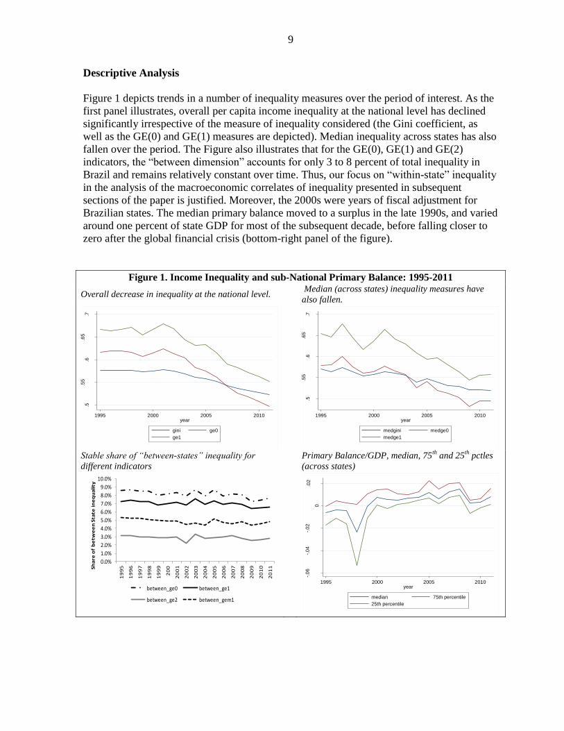
Descriptive Analysis
Figure 1 depicts trends in a number of inequality measures over the period of interest. As the
first panel illustrates, overall per capita income inequality at the national level has declined
significantly irrespective of the measure of inequality considered (the Gini coefficient, as
well as the GE(0) and GE(1) measures are depicted). Median inequality across states has also
fallen over the period. The Figure also illustrates that for the GE(0), GE(1) and GE(2)
indicators, the “between dimension” accounts for only 3 to 8 percent of total inequality in
Brazil and remains relatively constant over time. Thus, our focus on “within-state” inequality
in the analysis of the macroeconomic correlates of inequality presented in subsequent
sections of the paper is justified. Moreover, the 2000s were years of fiscal adjustment for
Brazilian states. The median primary balance moved to a surplus in the late 1990s, and varied
around one percent of state GDP for most of the subsequent decade, before falling closer to
zero after the global financial crisis (bottom-right panel of the figure).
Figure 1. Income Inequality and sub-National Primary Balance: 1995-2011
Overall decrease in inequality at the national level. Median (across states) inequality measures have
also fallen.
Stable share of “between-states” inequality for
different indicators
Primary Balance/GDP, median, 75th
and 25th
pctles
(across states)
.5.5
5.6
.65
.7
1995 2000 2005 2010year
gini ge0
ge1
.5.5
5.6
.65
.7
1995 2000 2005 2010year
medgini medge0
medge1
0.0%
1.0%
2.0%
3.0%
4.0%
5.0%
6.0%
7.0%
8.0%
9.0%
10.0%
19
95
19
96
19
97
19
98
19
99
20
0
20
01
20
02
20
03
20
04
20
05
20
06
20
07
20
08
20
09
20
10
20
11Sh
are
of
be
twe
en
Sta
te i
ne
qu
ali
ty
between_ge0 between_ge1
between_ge2 between_gem1
-.0
6-.
04
-.0
2
0
.02
pri
mary
ba
lance
1995 2000 2005 2010year
median 75th percentile
25th percentile

10
V. MODELING APPROACH AND RESULTS
We follow a parsimonious empirical specification summarized in Equation 1 for 1,...,i N
states; 1,...,t T time periods and 1,...,m M control variables. The variable ity represents
one of the PNAD-based income inequality measure (we focus on the log of the Gini index) at
the state level; Δpb are changes in the cyclically-adjusted primary balance as a share of state
GDP (a measure of the fiscal stance); X is a set of controls; i are state-specific fixed-effects;
it is the error term, assumed to be white noise. When estimating equation 1, we also include
time dummies and a time trend in the specification.
,, 1 , 1 , , 1
1
, ,
,
t
M
m i ti t i t m i tm
i t i i t
i ty y pb X u
u
(1)
We consider the following macroeconomic and fiscal variables as controls in the baseline
regressions: the employment rate; the state-level GDP per capita growth rate; inflation
(measured by changes in the state GDP deflator); state and municipal “social” expenditure as
a share of state-GDP; Federal social transfers as a share of state GDP. See annex A for data
definitions and sources.
The construction of the cyclically-adjusted primary balance warrants a more detailed
explanation. We focus on adjustments of revenue and expenditure to the output gap and do
not consider the impact of equity or commodity price fluctuations. We believe that this is
justified given the results discussed in IMF (2011) suggesting that, at the national level,
revenue elasticites relative to cycles in equity and commodity prices appear to be very small.
We follow the “aggregated method” described in Bornhorst and others (2011) and focus on
the sensitivity of aggregate revenues and expenditures to the output gap at the state-level.
The results presented in subsequently sections continue to hold when we consider the
unadjusted primary balance.
The output gap is calculated by applying the Hodrick-Prescott filter to the log of the real
state-level GDP series with a smoothing parameter of 6.25, as suggested by Ravn and Uhlig
(2002) for annual data. We experimented with different smoothing parameters that might be
more appropriate for cycles in developing countries, which tend to have shorter duration
(Rand and Tarp, 2002), as well as with the use of alternative filters (for example, the
Christiano and Fitzgerald filter), but found that these variations in the methodology do not
substantially affect the estimates of the output gap.
We use the revenue and expenditure elasticities estimated by Arena and Revilla (2009) for
Brazilian states over the period 1991-2006. These authors estimate a total revenue elasticity
11
of around 1.7 and total expenditure elasticity of 1.3.6 Thus, the cyclically-adjusted primary
balance as a share of state GDP is given by Equation 2, where R denotes state-level primary
revenue, G denotes state-level primary expenditures, Y is state-GDP, PY is potential output,
and are the respective elasticities.
R GP P
t t t tt
t t t t
R Y G Ycapb
Y Y Y Y (2)
Our measure of the fiscal stance differs from the “action-based” fiscal consolidation
measures constructed by Devries and others (2011) and used in several papers in the
literature for OECD economies. The construction of a similar “action-based” measure for
Brazilian states is more difficult given that historical policy documents providing information
on discretionary changes in taxes and expenditures are not readily available at the sub-
national level. Furthermore, we are also considering the effects of gradual continuous
adjustment in our analysis rather than focusing exclusively on large consolidation episodes,
as it is frequently done when analyzing fiscal consolidation (Alesina and Ardagna, 2012).
Finally, a structurally-adjusted primary balance (i.e. the primary balance adjusted not only
for cyclical fluctuations, but also for one-off fiscal operations) would provide a better
measure of the fiscal stance. However, it was not possible to remove one-off fiscal operations
at the state-level in a consistent and systematic way due to lack of information and
accounting challenges. In any case, one-off fiscal operations are more likely to occur at the
federal level and in this context; we believe that the use of the cyclically-adjusted balance is
adequate.
Descriptive statistics for selected variables are presented in Annex B. We test for unit root
and cross-sectional dependence in the main variables (Annex C). The Pesaran (2007) test,
which allows for cross-sectional heterogeneity and models cross-sectional dependence as an
unobserved common factor, suggests that all variables are stationary and therefore
conventional panel techniques might be appropriate for the analysis. Nevertheless, there is
strong evidence that cross sectional dependence is a problem, as indicated by the Pesaran
(2004) test.
Cross-sectional dependence can arise because of spill-overs and/or spatial effects among the
states or because of the presence of common (unobserved) factors. Estimators conventionally
used in panel data analysis require the assumption of cross-sectional independence across
panel members. In the presence of cross-sectionally correlated error terms, these methods do
not produce consistent estimates and can lead to incorrect inference (Kapetanios, Pesaran and
Yamagata, 2011). We attempt to mitigate cross-sectional dependence through different
strategies.
6 Our results still hold when we assume a unit elasticity for revenues and a zero elasticity for expenditures as it
is commonly done in the literature.
12
Fixed Effects Models
We first present results of the estimation of Equation 1 using fixed-effects models that take
into account state characteristics that are time invariant. In order to mitigate possible
endogeneity problems, we use lagged values of the control variables and therefore assume
that they are weakly exogenous. We also address cross-sectional dependence problems by
including time effects in the regressions and by using Driscoll and Kraay (1998) corrected
standard errors.
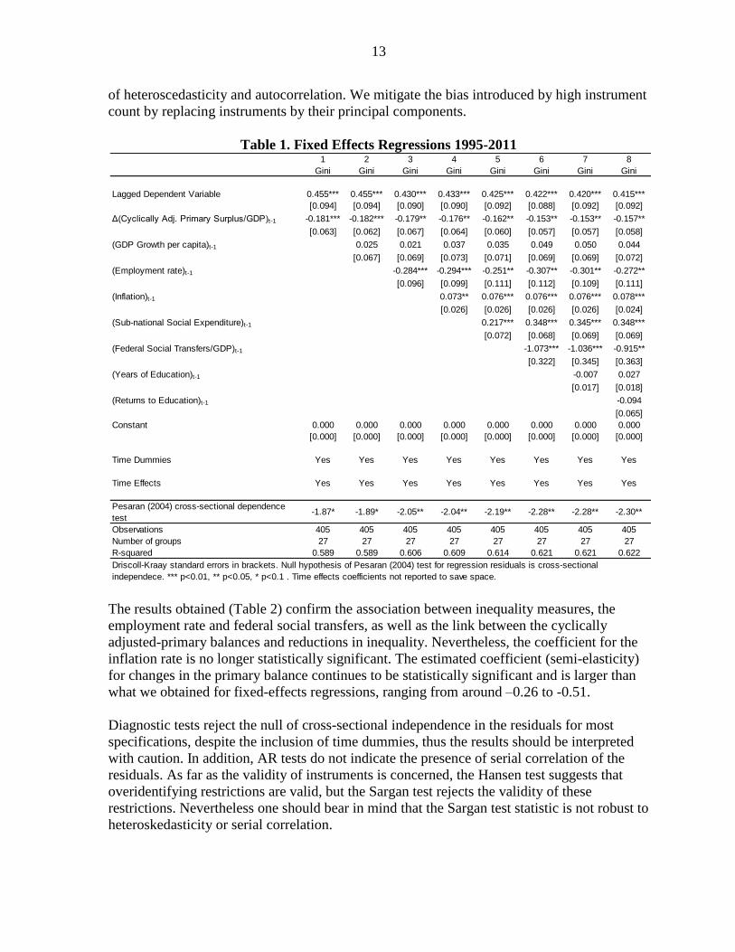
The results presented in Table 1 indicate that the employment rate is an important factor in
explaining inequality over the period. Furthermore, both real GDP per capita growth and the
inflation rate are linked to increases in inequality, but only the coefficients obtained for the
inflation rate are statistically significant, mirroring some of the results of the literature. This
highlights the importance of macroeconomic stabilization in inequality reduction, a well
established result in the Brazilian context.
More importantly for our purposes, fiscal variables seem to matter. Somewhat intriguingly, a
tighter fiscal stance is associated with less inequality. In addition, as expected, the highly
progressive social transfers at the federal level are strongly associated with reductions in
inequality with economically large coefficients. Finally, the level of social expenditures at
the state and municipal level appears to be associated with higher levels of inequality with
positive and statistically significant coefficients for all specifications, in line with the results
obtained by Lim and McNelis (2014)7 for Latin American countries and with results by
Ferreira, Leite and Ravaillon (2010) for Brazil.8
The effect of changes in the cyclically-adjusted primary balance remains significant when we
control for average years of education and average returns to education at the state level
(specifications 7 and 8 in the Table). The short-run coefficients for the effects of changes in
the primary surplus as a share of GDP on inequality range from -0.18 to -0.15 (the long-run
effects are around -0.4). These coefficients can be interpreted as semi-elasticities (note that
the dependent variable is expressed in logs).
GMM Estimation
It is possible that the results obtained with fixed effects specifications are due to
shortcomings in statistical techniques. Hence we re-estimate the models using GMM
techniques, namely the system (Blundell-Bond) GMM estimator (see Roodman, 2009 for a
discussion), which allow us to handle the potential endogeneity of some regressors by using
lagged values of these variables as instruments. We transform instruments using forward
orthogonal deviations and present robust standard errors, which are consistent in the presence
7 One should note that Lim and McNelis focus on overall spending rather than social spending and use country-
level data.
8 Ferreira, Leite and Ravaillon focus on the determinants of poverty reduction rather than inequality.
13
of heteroscedasticity and autocorrelation. We mitigate the bias introduced by high instrument
count by replacing instruments by their principal components.
Table 1. Fixed Effects Regressions 1995-2011
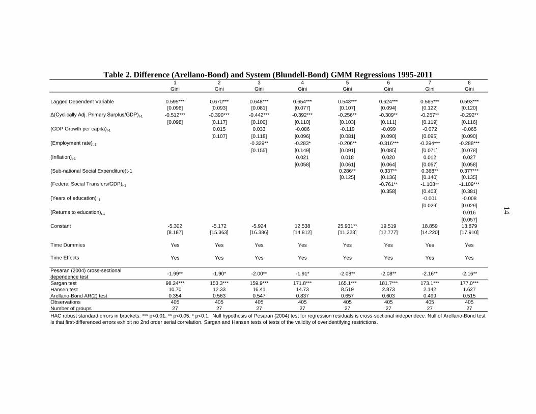
The results obtained (Table 2) confirm the association between inequality measures, the
employment rate and federal social transfers, as well as the link between the cyclically
adjusted-primary balances and reductions in inequality. Nevertheless, the coefficient for the
inflation rate is no longer statistically significant. The estimated coefficient (semi-elasticity)
for changes in the primary balance continues to be statistically significant and is larger than
what we obtained for fixed-effects regressions, ranging from around –0.26 to -0.51.
Diagnostic tests reject the null of cross-sectional independence in the residuals for most
specifications, despite the inclusion of time dummies, thus the results should be interpreted
with caution. In addition, AR tests do not indicate the presence of serial correlation of the
residuals. As far as the validity of instruments is concerned, the Hansen test suggests that
overidentifying restrictions are valid, but the Sargan test rejects the validity of these
restrictions. Nevertheless one should bear in mind that the Sargan test statistic is not robust to
heteroskedasticity or serial correlation.
1 2 3 4 5 6 7 8
Gini Gini Gini Gini Gini Gini Gini Gini
Lagged Dependent Variable 0.455*** 0.455*** 0.430*** 0.433*** 0.425*** 0.422*** 0.420*** 0.415***
[0.094] [0.094] [0.090] [0.090] [0.092] [0.088] [0.092] [0.092]
Δ(Cyclically Adj. Primary Surplus/GDP)t-1 -0.181*** -0.182*** -0.179** -0.176** -0.162** -0.153** -0.153** -0.157**
[0.063] [0.062] [0.067] [0.064] [0.060] [0.057] [0.057] [0.058]
(GDP Growth per capita)t-1 0.025 0.021 0.037 0.035 0.049 0.050 0.044
[0.067] [0.069] [0.073] [0.071] [0.069] [0.069] [0.072]
(Employment rate)t-1 -0.284*** -0.294*** -0.251** -0.307** -0.301** -0.272**
[0.096] [0.099] [0.111] [0.112] [0.109] [0.111]
(Inflation)t-1 0.073** 0.076*** 0.076*** 0.076*** 0.078***
[0.026] [0.026] [0.026] [0.026] [0.024]
(Sub-national Social Expenditure)t-1 0.217*** 0.348*** 0.345*** 0.348***
[0.072] [0.068] [0.069] [0.069]
(Federal Social Transfers/GDP)t-1 -1.073*** -1.036*** -0.915**
[0.322] [0.345] [0.363]
(Years of Education)t-1 -0.007 0.027
[0.017] [0.018]
(Returns to Education)t-1 -0.094
[0.065]
Constant 0.000 0.000 0.000 0.000 0.000 0.000 0.000 0.000
[0.000] [0.000] [0.000] [0.000] [0.000] [0.000] [0.000] [0.000]
Time Dummies Yes Yes Yes Yes Yes Yes Yes Yes
Time Effects Yes Yes Yes Yes Yes Yes Yes Yes
Pesaran (2004) cross-sectional dependence
test-1.87* -1.89* -2.05** -2.04** -2.19** -2.28** -2.28** -2.30**
Observations 405 405 405 405 405 405 405 405
Number of groups 27 27 27 27 27 27 27 27
R-squared 0.589 0.589 0.606 0.609 0.614 0.621 0.621 0.622
Driscoll-Kraay standard errors in brackets. Null hypothesis of Pesaran (2004) test for regression residuals is cross-sectional
independece. *** p<0.01, ** p<0.05, * p<0.1 . Time effects coefficients not reported to save space.
14
Table 2. Difference (Arellano-Bond) and System (Blundell-Bond) GMM Regressions 1995-2011
1 2 3 4 5 6 7 8
Gini Gini Gini Gini Gini Gini Gini Gini
Lagged Dependent Variable 0.595*** 0.670*** 0.648*** 0.654*** 0.543*** 0.624*** 0.565*** 0.593***
[0.096] [0.093] [0.081] [0.077] [0.107] [0.094] [0.122] [0.120]
Δ(Cyclically Adj. Primary Surplus/GDP)t-1 -0.512*** -0.390*** -0.442*** -0.392*** -0.256** -0.309** -0.257** -0.292**
[0.098] [0.117] [0.100] [0.110] [0.103] [0.111] [0.119] [0.116]
(GDP Growth per capita)t-1 0.015 0.033 -0.086 -0.119 -0.099 -0.072 -0.065
[0.107] [0.118] [0.096] [0.081] [0.090] [0.095] [0.090]
(Employment rate)t-1 -0.329** -0.283* -0.206** -0.316*** -0.294*** -0.288***
[0.155] [0.149] [0.091] [0.085] [0.071] [0.078]
(Inflation)t-1 0.021 0.018 0.020 0.012 0.027
[0.058] [0.061] [0.064] [0.057] [0.058]
(Sub-national Social Expenditure)t-1 0.286** 0.337** 0.368** 0.377***
[0.125] [0.136] [0.140] [0.135]
(Federal Social Transfers/GDP)t-1 -0.761** -1.108** -1.109***
[0.358] [0.403] [0.381]
(Years of education)t-1 -0.001 -0.008
[0.029] [0.029]
(Returns to education)t-1 0.016
[0.057]
Constant -5.302 -5.172 -5.924 12.538 25.931** 19.519 18.859 13.879
[8.187] [15.363] [16.386] [14.812] [11.323] [12.777] [14.220] [17.910]
Time Dummies Yes Yes Yes Yes Yes Yes Yes Yes
Time Effects Yes Yes Yes Yes Yes Yes Yes Yes
Pesaran (2004) cross-sectional
dependence test-1.99** -1.90* -2.00** -1.91* -2.08** -2.08** -2.16** -2.16**
Sargan test 98.24*** 153.3*** 159.9*** 171.8*** 165.1*** 181.7*** 173.1*** 177.0***
Hansen test 10.70 12.33 16.41 14.73 8.519 2.873 2.142 1.627
Arellano-Bond AR(2) test 0.354 0.563 0.547 0.837 0.657 0.603 0.499 0.515
Observations 405 405 405 405 405 405 405 405
Number of groups 27 27 27 27 27 27 27 27
HAC robust standard errors in brackets. *** p<0.01, ** p<0.05, * p<0.1. Null hypothesis of Pesaran (2004) test for regression residuals is cross-sectional independece. Null of Arellano-Bond test
is that first-differenced errors exhibit no 2nd order serial correlation. Sargan and Hansen tests of tests of the validity of overidentifying restrictions.
15
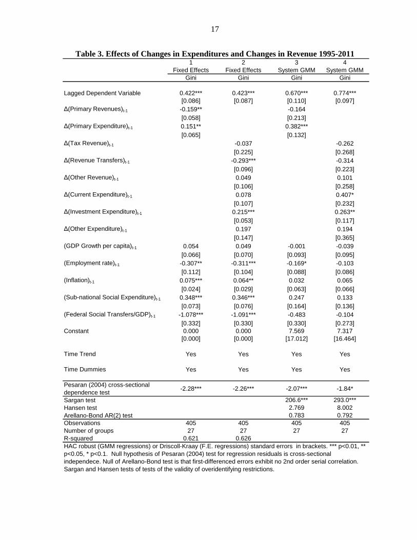
Disentangling the Effects of Changes in Expenditures and Changes in Revenue
As we have seen in previous sections, a number of papers in the cross-country literature on
fiscal consolidations at the national level tend to find different effects on inequality
depending on whether the consolidation is “expenditure-based” or “revenue-based”. In this
section we will explore these differential channels for the Brazilian case by separately
including changes in revenues and changes in primary expenditures in our regressions rather
than focusing on the cyclically adjusted primary balance. We do not attempt to describe the
precise mechanism driving these results, but to shed light on possible candidates for
transmission channels.
The evidence at the national level for Brazil and other Latin American countries points to a
greater reliance on indirect (regressive) taxes relative to income taxes, which would suggest
that higher primary surpluses driven by higher tax revenues would tend to be associated with
increases in inequality (Bastagli, Coady and Gupta, 2012 and Goni, Lopez and Serven,
2011). On the other hand, the evidence at the national level also indicates that a large share of
social spending is captured by the better off, and thus reductions of these expenditures would
not necessarily lead to increases in inequality.
Prior to presenting the regression results, it is important to note that revenues have played an
influential role in those years in which the state-level primary surpluses experienced a
positive change. Expenditures, on the other hand, have been relatively more influential in
those years in which the state-level primary surpluses experienced negative changes. Hence,
fluctuations of the overall fiscal adjustment process embed changing roles for revenue and
expenditure. Also, from a descriptive perspective, the fiscal adjustment process at the state-
level appears to have a relatively stronger revenue-side component on aggregate, though this
pattern can vary significantly by state.
The regression results are presented in Table 3. In fixed-effects regressions (specification 1 in
the Table), changes in revenues are negatively associated with inequality, whereas changes in
primary expenditures present a positive association. Further disaggregation of revenues and
expenditures suggests that these results are driven by changes in revenues linked to revenue
transfers to states9 and by changes in investment expenditure (specification 2), with
coefficients for these variables being significant at the 1 percent level. These relations hold
with the same signs for GMM regressions as well, nevertheless only changes in primary
expenditures are statistically significant. Cross-sectional dependence of the residuals
continues to be a problem in GMM regressions.
9 Note that the federal revenue transfers go to state governments, whereas federal social transfers also
considered in the regressions are direct cash transfers to households, thus these components have very different
implications for inequality. The bulk of revenue transfers originate from the “States’ Participation Fund”, which
comprises revenues from income taxes and the IPI tax on manufactured products (21.5% of the revenues linked
to these taxes is allocated to the Fund). States with lower GDP per capita receive a relatively larger share of the
transfers.
16
In this context, we can conclude that revenue increases in Brazilian states were not typically
linked to increases in inequality over the period of analysis. Furthermore, reductions in
primary expenditures also do not seem to have had deleterious impacts on inequality
measures. The behavior of revenue transfers to states and investment expenditure seem to be
particularly important to explain these results. Changes in revenues linked to revenue
transfers are associated with reductions in “within-state” income inequality, though between-
state inequality has remained broadly stable (as discussed previously). The rules that govern
federal revenue transfers to states in Brazil do favor poorer states (in terms of GDP per
capita), which tend to present higher inequality indicators as well.
Changes in investment expenditure also seem to have played a role in inequality dynamics,
but in the direction of increasing inequality. As argued by Lim and McNelis (2014), capital
spending (especially infrastructure spending) enhances the returns to capital and might
contribute to increase inequality. In the case of Brazil, public investment does appear to have
an infrastructure bias. Evidently, our results do not show that infrastructure investment has a
permanent negative impact on inequality.
Finally, it is important to note that the scope for efficiency gains in revenue mobilization at
the state-level a decade ago were substantial, so it would have been plausible for states to
raise revenues without necessarily exacerbating existing inefficiencies. In addition, current
public spending could also have been captured by the better off, and thus controlling the
growth of these expenditures would not necessarily lead to increases in inequality. Overall,
our results are consistent with the view that the observed fiscal adjustment process has
contributed to a better economic environment and to a more judicious and efficient use of
public resources.
One important caveat regarding the disaggregated results is that the quality of the fiscal
information deteriorates as one considers the breakdown of revenues and expenditures at the
state level. This is due to potential misclassification and lack of harmonized classification
practices across states. The primary surplus measure is significantly less affected by such
issues. The primary balance is also calculated by the Central Bank using financing
information and by the Treasury using information above the line.
17
Table 3. Effects of Changes in Expenditures and Changes in Revenue 1995-2011
1 2 3 4
Fixed Effects Fixed Effects System GMM System GMM
Gini Gini Gini Gini
Lagged Dependent Variable 0.422*** 0.423*** 0.670*** 0.774***
[0.086] [0.087] [0.110] [0.097]
Δ(Primary Revenues)t-1 -0.159** -0.164
[0.058] [0.213]
Δ(Primary Expenditure)t-1 0.151** 0.382***
[0.065] [0.132]
Δ(Tax Revenue)t-1 -0.037 -0.262
[0.225] [0.268]
Δ(Revenue Transfers)t-1 -0.293*** -0.314
[0.096] [0.223]
Δ(Other Revenue)t-1 0.049 0.101
[0.106] [0.258]
Δ(Current Expenditure)t-1 0.078 0.407*
[0.107] [0.232]
Δ(Investment Expenditure)t-1 0.215*** 0.263**
[0.053] [0.117]
Δ(Other Expenditure)t-1 0.197 0.194
[0.147] [0.365]
(GDP Growth per capita)t-1 0.054 0.049 -0.001 -0.039
[0.066] [0.070] [0.093] [0.095]
(Employment rate)t-1 -0.307** -0.311*** -0.169* -0.103
[0.112] [0.104] [0.088] [0.086]
(Inflation)t-1 0.075*** 0.064** 0.032 0.065
[0.024] [0.029] [0.063] [0.066]
(Sub-national Social Expenditure)t-1 0.348*** 0.346*** 0.247 0.133
[0.073] [0.076] [0.164] [0.136]
(Federal Social Transfers/GDP)t-1 -1.078*** -1.091*** -0.483 -0.104
[0.332] [0.330] [0.330] [0.273]
Constant 0.000 0.000 7.569 7.317
[0.000] [0.000] [17.012] [16.464]
Time Trend Yes Yes Yes Yes
Time Dummies Yes Yes Yes Yes
Pesaran (2004) cross-sectional
dependence test-2.28*** -2.26*** -2.07*** -1.84*
Sargan test 206.6*** 293.0***
Hansen test 2.769 8.002
Arellano-Bond AR(2) test 0.783 0.792
Observations 405 405 405 405
Number of groups 27 27 27 27
R-squared 0.621 0.626
HAC robust (GMM regressions) or Driscoll-Kraay (F.E. regressions) standard errors in brackets. *** p<0.01, **
p<0.05, * p<0.1. Null hypothesis of Pesaran (2004) test for regression residuals is cross-sectional
independece. Null of Arellano-Bond test is that first-differenced errors exhibit no 2nd order serial correlation.
Sargan and Hansen tests of tests of the validity of overidentifying restrictions.
18
Fiscal Adjustment and “Shared Prosperity”
The World Bank has recently advocated the notion of “shared prosperity” as a major policy
goal in order to address the shortcomings of standard measures of economic development
(Word Bank, 2013). The World Bank’s shared prosperity indicator is defined as the growth
rate of the income of the bottom 40 percent of the income distribution. Contrary to indicators
of economic development from national accounts (such as GDP growth), improvements in
share prosperity require growth to be inclusive of the less well-off segments of the population
(Basu, 2013).
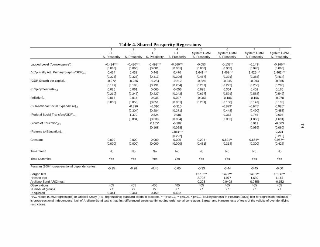
We examine the links between fiscal policy at the state-level and shared prosperity in Brazil.
The results obtained when regressing the first difference of the log income of the bottom 40
percent on our baseline control variables are presented in Table 4. Since the dependent
variable is now a growth rate, we modify Equation 2 and include the lagged level of the log
of the income of the bottom 40 percent as a control variable to capture convergence effects
(see equation 3). Time dummies were also included, but not a time trend.
,, 1 , 1 , , 1
1
, ,
, 40
t
M
m i ti t i t m i tm
i t i i t
i tSP Incb pb X u
u
(3)
The results are mixed for the main variable of interest. The coefficients for changes in the
cyclically-adjusted primary balance are positive, but not statistically significant in fixed-
effects regressions. Nevertheless, the coefficients are highly significant for all GMM
specifications (with semi-elasticities ranging from 1.4 to 1.6). Diagnostic tests do not indicate
that cross-sectional dependence is a problem for these models. Overall, except for the
convergence term, the other control variables included do not seem to present a robust
statistically significant association with our shared prosperity measure, which indicates that
exploring the correlates of shared prosperity at the sub-national level remains an interesting
avenue for further research.
Summing up, in all specifications presented in this section, a tighter fiscal stance at the sub-
national level is negatively associated with inequality and positively associated with our
measure of shared prosperity. Nevertheless, in what concerns the shared prosperity
regressions, the coefficient of the change in the cyclically-adjusted primary balance is not
statistically significant in fixed-effect specifications. In none of the specifications the tighter
fiscal stance is linked to a deterioration in inequality.
These conclusions contrast with the literature based on cross-country data that examines the
link between fiscal consolidation and inequality at the national level. These differences could
be explained by the fact that several of these studies employ measures of fiscal adjustment
that are different from the ones used here. The difference could also be linked to the
definition of income used to measure inequality. Some studies use measures based on
disposable income, while in Brazil we use income after transfers and before taxes.
19
Table 4. Shared Prosperity Regressions
1 2 3 4 5 6 7 8
F.E. F.E. F.E. F.E. System GMM System GMM System GMM System GMM
S. Prosperity S. Prosperity S. Prosperity S. Prosperity S. Prosperity S. Prosperity S. Prosperity S. Prosperity
Lagged Level ("convergence") -0.424*** -0.430*** -0.492*** -0.566*** -0.053 -0.138** -0.143* -0.166**
[0.063] [0.066] [0.081] [0.081] [0.038] [0.062] [0.070] [0.068]
Δ(Cyclically Adj. Primary Surplus/GDP)t-1 0.464 0.438 0.443 0.470 1.641*** 1.468*** 1.425*** 1.462***
[0.325] [0.328] [0.313] [0.309] [0.457] [0.391] [0.388] [0.414]
(GDP Growth per capita)t-1 -0.272 -0.286 -0.284 -0.212 -0.324 -0.245 -0.293 -0.356
[0.197] [0.198] [0.191] [0.204] [0.287] [0.272] [0.256] [0.285]
(Employment rate)t-1 0.026 0.061 0.060 -0.056 0.095 0.364 0.402 0.165
[0.210] [0.243] [0.227] [0.242] [0.677] [0.591] [0.588] [0.542]
(Inflation)t-1 0.017 0.014 0.038 0.027 -0.083 -0.186 -0.156 -0.078
[0.056] [0.055] [0.051] [0.051] [0.231] [0.168] [0.147] [0.190]
(Sub-national Social Expenditure)t-1 -0.396 -0.310 -0.315 -0.879* -0.945* -0.926*
[0.304] [0.284] [0.271] [0.448] [0.490] [0.456]
(Federal Social Transfers/GDP)t-1 1.379 0.824 -0.081 0.362 0.746 0.608
[0.834] [0.638] [0.984] [2.052] [1.866] [1.691]
(Years of Education)t-1 0.185* -0.102 0.011 -0.083
[0.108] [0.068] [0.059] [0.060]
(Returns to Education)t-1 0.881*** 0.231
[0.222] [0.213]
Constant 0.000 0.000 0.000 0.000 0.294 0.691** 0.664** 0.967**
[0.000] [0.000] [0.000] [0.000] [0.431] [0.314] [0.300] [0.425]
Time Trend No No No No No No No No
Time Dummies Yes Yes Yes Yes Yes Yes Yes Yes
Pesaran (2004) cross-sectional dependence test-0.15 -0.26 -0.45 -0.65 -0.33 -0.44 -0.45 -0.60
Sargan test 127.8*** 142.2** 149.1** 161.4***
Hansen test 3.728 1.977 1.639 1.167
Arellano-Bond AR(2) test 0.223 0.0408 -0.0356 -0.152
Observations 405 405 405 405 405 405 405 405
Number of groups 27 27 27 27 27 27 27 27
R-squared 0.441 0.444 0.459 0.482
HAC robust (GMM regressions) or Driscoll-Kraay (F.E. regressions) standard errors in brackets. *** p<0.01, ** p<0.05, * p<0.1. Null hypothesis of Pesaran (2004) test for regression residuals
is cross-sectional independece. Null of Arellano-Bond test is that first-differenced errors exhibit no 2nd order serial correlation. Sargan and Hansen tests of tests of the validity of overidentifying
restrictions.

20
Nevertheless, we believe that the bulk of the differences in results are explained by
differences in structural characteristics (fiscal, social, and economic). Finally, it is worth
noting that all measures of inequality used in this paper came from the same survey, which is
conducted using the exact same questionnaire, with the same field work protocols, and using
the same period of reference. As Beegle and others (2012) rigorously demonstrate survey
design and implementation effects can have significant impacts on the final indicators, which
can confound any cross country analysis in this field.
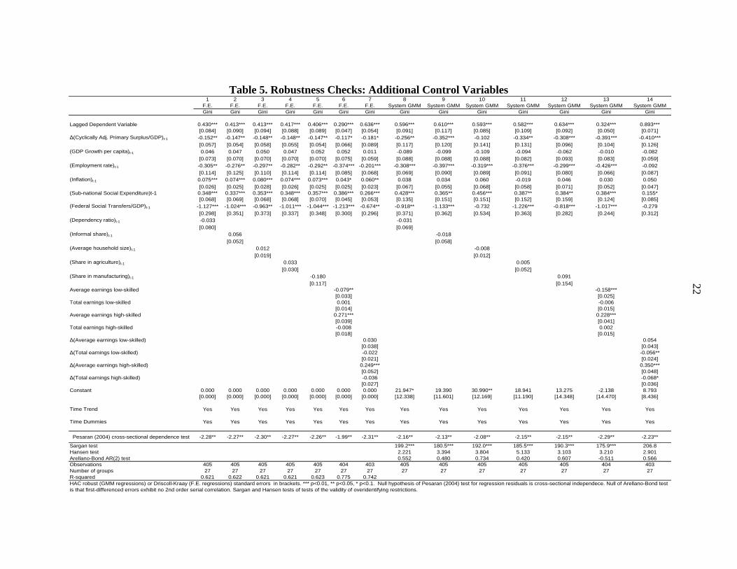
VI. ROBUSTNESS CHECKS
In this section, we discuss a number of alternative specifications. We start by estimating
regressions including additional control variables (Table 5), namely the share of prime-age
workers in the informal sector, the share of employment in agriculture, the share of
employment in manufacturing, as well as some demographic variables (the dependency ratio
and the average household size). Specifications 1 to 7 of the Table present results for fixed
effects regressions and the columns 8 to 14 present results for system GMM specifications.
None of the additional control variables present statistically significant coefficients, but
otherwise the results are broadly similar to the ones obtained previously. The coefficients for
the employment rate, federal direct transfers and the primary balance being negative and
statistically significant in most specifications (except for one in the case of the latter
variable). In addition, we estimated models that include the share of employment in all
sectors (excluding manufacturing) and our benchmark results did not change (results are
available upon request).
Moreover, we also considered specifications that include the log of the average labor income
of low-skilled workers (defined as workers with 8 years of education or less) and the log of
average labor income of high-skilled workers as well as the total labor income of low and
high-skilled workers as control variables. Specifications 6 and 13 include these additional
control variables in levels using fixed effects and the GMM estimators respectively, whereas
specifications 7 and 14 consider the first differences.
As expected, the coefficient for average earnings of high-skilled workers is positive and
significant and the earnings for low-skilled workers present a negative coefficient. More
importantly for our purposes, the coefficient for the primary balance continues to be negative
and significant in all specifications, although its statistical significance is reduced to the 10%
level in fixed-effects regressions (but not in GMM ones).
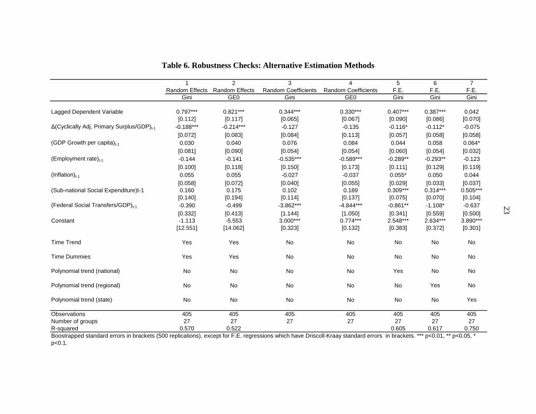
In Table 6 we consider alternative estimation methods. The first two columns present
estimates from random effects models. Overall, these models do not perform well (in the
sense that most variables are not statistically significant), but the link between changes in the
cyclically-adjusted primary balance and inequality remains negative and statistically
significant. We also consider models that allow both the intercept and slope coefficients to
vary across panel members, following the random coefficient model proposed by Swamy
(1970). We use bootstrapping to obtain robust standard errors in this case and present

21
specifications with and without a deterministic trend. For these models, the coefficient for the
primary balance continues to be negative, but is no longer statistically significant.
We also experimented with specifications that model deterministic components (i.e. time
trends and time effects) in a different way. We estimated regressions including national,
regional and state-level polynomial time trends and results are qualitatively similar to those
already presented (see specifications 5 to 7 in the Table). Even if the statistical significance
of the results for the primary balance is reduced (as we lose degrees of freedom), the
coefficient for these variables remains negative in all specifications.
Overall, the robustness checks confirm that there is no evidence that fiscal adjustment at the
sub-national level is positively linked to inequality in Brazil. On the contrary, for several
specifications, changes in the primary balance are negatively associated with inequality
measures with statistically significant coefficients.
22
Table 5. Robustness Checks: Additional Control Variables
1 2 3 4 5 6 7 8 9 10 11 12 13 14
F.E. F.E. F.E. F.E. F.E. F.E. F.E. System GMM System GMM System GMM System GMM System GMM System GMM System GMM
Gini Gini Gini Gini Gini Gini Gini Gini Gini Gini Gini Gini Gini Gini
Lagged Dependent Variable 0.430*** 0.413*** 0.413*** 0.417*** 0.406*** 0.290*** 0.636*** 0.596*** 0.610*** 0.593*** 0.582*** 0.634*** 0.324*** 0.893***
[0.084] [0.090] [0.094] [0.088] [0.089] [0.047] [0.054] [0.091] [0.117] [0.085] [0.109] [0.092] [0.050] [0.071]
Δ(Cyclically Adj. Primary Surplus/GDP)t-1 -0.152** -0.147** -0.148** -0.148** -0.147** -0.117* -0.181* -0.256** -0.352*** -0.102 -0.334** -0.308*** -0.391*** -0.410***
[0.057] [0.054] [0.058] [0.055] [0.054] [0.066] [0.089] [0.117] [0.120] [0.141] [0.131] [0.096] [0.104] [0.126]
(GDP Growth per capita)t-1 0.046 0.047 0.050 0.047 0.052 0.052 0.011 -0.089 -0.099 -0.109 -0.094 -0.062 -0.010 -0.082
[0.073] [0.070] [0.070] [0.070] [0.070] [0.075] [0.059] [0.088] [0.088] [0.088] [0.082] [0.093] [0.083] [0.059]
(Employment rate)t-1 -0.305** -0.276** -0.297** -0.282** -0.292** -0.374*** -0.201*** -0.308*** -0.397*** -0.319*** -0.376*** -0.299*** -0.426*** -0.092
[0.114] [0.125] [0.110] [0.114] [0.114] [0.085] [0.068] [0.069] [0.090] [0.089] [0.091] [0.080] [0.066] [0.087]
(Inflation)t-1 0.075*** 0.074*** 0.080*** 0.074*** 0.073*** 0.043* 0.060** 0.038 0.034 0.060 -0.019 0.046 0.030 0.050
[0.026] [0.025] [0.028] [0.026] [0.025] [0.025] [0.023] [0.067] [0.055] [0.068] [0.058] [0.071] [0.052] [0.047]
(Sub-national Social Expenditure)t-1 0.348*** 0.337*** 0.353*** 0.348*** 0.357*** 0.386*** 0.266*** 0.428*** 0.365** 0.456*** 0.387** 0.384** 0.384*** 0.155*
[0.068] [0.069] [0.068] [0.068] [0.070] [0.045] [0.053] [0.135] [0.151] [0.151] [0.152] [0.159] [0.124] [0.085]
(Federal Social Transfers/GDP)t-1 -1.127*** -1.024*** -0.963** -1.011*** -1.044*** -1.213*** -0.674** -0.918** -1.133*** -0.732 -1.226*** -0.818*** -1.017*** -0.279
[0.298] [0.351] [0.373] [0.337] [0.348] [0.300] [0.296] [0.371] [0.362] [0.534] [0.363] [0.282] [0.244] [0.312]
(Dependency ratio)t-1 -0.033 -0.031
[0.080] [0.069]
(Informal share)t-1 0.056 -0.018
[0.052] [0.058]
(Average household size)t-1 0.012 -0.008
[0.019] [0.012]
(Share in agriculture)t-1 0.033 0.005
[0.030] [0.052]
(Share in manufacturing)t-1 -0.180 0.091
[0.117] [0.154]
Average earnings low-skilled -0.079** -0.158***
[0.033] [0.025]
Total earnings low-skilled 0.001 -0.006
[0.014] [0.015]
Average earnings high-skilled 0.271*** 0.228***
[0.039] [0.041]
Total earnings high-skilled -0.008 0.002
[0.018] [0.015]
Δ(Average earnings low-skilled) 0.030 0.054
[0.038] [0.043]
Δ(Total earnings low-skilled) -0.022 -0.056**
[0.021] [0.024]
Δ(Average earnings high-skilled) 0.249*** 0.350***
[0.052] [0.048]
Δ(Total earnings high-skilled) -0.036 -0.068*
[0.027] [0.036]
Constant 0.000 0.000 0.000 0.000 0.000 0.000 0.000 21.947* 19.390 30.990** 18.941 13.275 -2.138 8.793
[0.000] [0.000] [0.000] [0.000] [0.000] [0.000] [0.000] [12.338] [11.601] [12.169] [11.190] [14.348] [14.470] [8.436]
Time Trend Yes Yes Yes Yes Yes Yes Yes Yes Yes Yes Yes Yes Yes Yes
Time Dummies Yes Yes Yes Yes Yes Yes Yes Yes Yes Yes Yes Yes Yes Yes
Pesaran (2004) cross-sectional dependence test -2.28** -2.27** -2.30** -2.27** -2.26** -1.99** -2.31** -2.16** -2.13** -2.08** -2.15** -2.15** -2.29** -2.23**
Sargan test 199.2*** 180.5*** 192.0*** 185.5*** 190.3*** 175.9*** 206.8
Hansen test 2.221 3.394 3.804 5.133 3.103 3.210 2.901
Arellano-Bond AR(2) test 0.552 0.480 0.734 0.420 0.607 -0.511 0.566
Observations 405 405 405 405 405 404 403 405 405 405 405 405 404 403
Number of groups 27 27 27 27 27 27 27 27 27 27 27 27 27 27
R-squared 0.621 0.622 0.621 0.621 0.623 0.775 0.742
HAC robust (GMM regressions) or Driscoll-Kraay (F.E. regressions) standard errors in brackets. *** p<0.01, ** p<0.05, * p<0.1. Null hypothesis of Pesaran (2004) test for regression residuals is cross-sectional independece. Null of Arellano-Bond test
is that first-differenced errors exhibit no 2nd order serial correlation. Sargan and Hansen tests of tests of the validity of overidentifying restrictions.
23
Table 6. Robustness Checks: Alternative Estimation Methods
1 2 3 4 5 6 7
Random Effects Random Effects Random Coefficients Random Coefficients F.E. F.E. F.E.
Gini GE0 Gini GE0 Gini Gini Gini
Lagged Dependent Variable 0.797*** 0.821*** 0.344*** 0.330*** 0.407*** 0.387*** 0.042
[0.112] [0.117] [0.065] [0.067] [0.090] [0.086] [0.070]
Δ(Cyclically Adj. Primary Surplus/GDP)t-1 -0.188*** -0.214*** -0.127 -0.135 -0.116* -0.112* -0.075
[0.072] [0.083] [0.084] [0.113] [0.057] [0.058] [0.058]
(GDP Growth per capita)t-1 0.030 0.040 0.076 0.084 0.044 0.058 0.064*
[0.081] [0.090] [0.054] [0.054] [0.060] [0.054] [0.032]
(Employment rate)t-1 -0.144 -0.141 -0.535*** -0.589*** -0.289** -0.293** -0.123
[0.100] [0.118] [0.150] [0.173] [0.111] [0.129] [0.119]
(Inflation)t-1 0.055 0.055 -0.027 -0.037 0.055* 0.050 0.044
[0.058] [0.072] [0.040] [0.055] [0.029] [0.033] [0.037]
(Sub-national Social Expenditure)t-1 0.160 0.175 0.102 0.189 0.309*** 0.314*** 0.505***
[0.140] [0.194] [0.114] [0.137] [0.075] [0.070] [0.104]
(Federal Social Transfers/GDP)t-1 -0.390 -0.499 -3.862*** -4.844*** -0.861** -1.108* -0.637
[0.332] [0.413] [1.144] [1.050] [0.341] [0.559] [0.500]
Constant -1.113 -5.553 3.000*** 0.774*** 2.548*** 2.634*** 3.890***
[12.551] [14.062] [0.323] [0.132] [0.383] [0.372] [0.301]
Time Trend Yes Yes No No No No No
Time Dummies Yes Yes No No No No No
Polynomial trend (national) No No No No Yes No No
Polynomial trend (regional) No No No No No Yes No
Polynomial trend (state) No No No No No No Yes
Observations 405 405 405 405 405 405 405
Number of groups 27 27 27 27 27 27 27
R-squared 0.570 0.522 0.605 0.617 0.750
Boostrapped standard errors in brackets (500 replications), except for F.E. regressions which have Driscoll-Kraay standard errors in brackets. *** p<0.01, ** p<0.05, *
p<0.1.
24
VII. CONCLUSIONS
In this paper, we find that a tighter fiscal stance in Brazilian states, measured by changes in
the cyclically-adjusted primary balance, does not seem to increase inequality over the period
1995–2011. This conclusion contrasts to the results of several papers that analyze the impact
of fiscal consolidations on inequality at the national level for OECD countries (Ball and
others, 2013). All measures of inequality considered in this paper came from the same survey
and therefore are not subject to “spurious” design and implementation effects that can
confound a cross-country analysis of heterogeneous surveys.
Our results also suggest that revenue increases in Brazilian states were not associated with
increases in inequality. In addition, reductions in primary expenditures do not seem to have
had deleterious impacts on inequality measures. Some further disaggregation indicates that
revenue increases due to revenue transfers to states are linked to decreases in inequality,
whereas changes in investment expenditure are positively linked to inequality measures.
Several robustness checks performed confirm that there is no evidence that fiscal adjustment
at the sub-national level is positively linked to inequality.
The different conclusions obtained relative to the rest of the literature could be explained by
differences in the institutional setting and in the structural characteristics of Brazilian states
relative to OECD economies, such as the importance of transfers of revenues. The paper does
not attempt to establish the precise mechanism at play, but possible differences driving the
result include: higher initial levels of inequality; lesser reliance on progressive taxation; the
absence of extensive social safety nets and other automatic stabilizers; scope to significantly
improve the efficiency of public spending and the quality of public services; and the
regressive nature of some forms of public expenditure at the state level.
Furthermore, fiscal adjustment at the state-level might also have been achieved through
efficiency gains both on the expenditure-side, but also in terms of revenue collection with no
discernible impact in terms of increasing inequality. In addition, greater fiscal discipline
could also have improved the investment climate within states, which facilitated job creation
and investment.
Future research could focus on drilling down on the mechanism linking the fiscal stance and
inequality dynamics. This would be important to ascertain where the relationship is likely to
be maintained over time as the country macroeconomic and social conditions evolve, thus
informing policy making more precisely. A central message, however, is that the results
linking fiscal adjustment to an increase in inequality in advanced economies cannot be easily
generalized to developing countries, given the Brazilian experience.
25
REFERENCES
Acemoglu, D., Johnson, S., Robinson, J. and Thaicharoen, Y., 2003, “Institutional Causes,
Macroeconomic Symptoms: Volatility, Crises and Growth,” Journal of Monetary
Economics, Vol. 50(1), pp. 49–123.
Afonso, A., Schuknecht, L. and Tanzi, V., 2010, “Income distribution Determinants and
Public Spending efficiency,” Journal of Economic Inequality, Vol. 8, pp. 367–389.
Aghion, P. Caroli, E. and Garcia-Penalosa, C., 1999, “Inequality and Growth: The
Perspective of New Growth Theories,” Journal of Economic Literature, Vol. 37(4),
pp. 1615–1660.
Agnello, L. and Sousa, R.M., 2012, “How does Fiscal Consolidation Impact on Income
Inequality,” Banque de France, Document de Travail No 382 (May).
Alesina, A. and Ardagna, S., 2012, “The Design of Fiscal Adjustments,” NBER Working
Paper 18423, September (Cambridge).
Arena, M. & Revilla, J.E., 2009, “Pro-cyclical Fiscal Policy in Brazil: Evidence from the
States,” World Bank Policy Research Working Paper 5144 (Washington: The World
Bank).
Azevedo, J. P., Davalos, M. E., Diaz-Bonilla, C., Atuesta, B. and Castaneda, R., 2013,
“Fifteen years of inequality in Latin America how have labor markets helped?” World
Bank Policy Research Working Paper 6384 (Washington: The World Bank).
Azevedo, J. P., Inchauste, G. and Sanfelice. V., 2013, “Decomposing the recent inequality
decline in Latin America,” World Bank Policy Research Working Paper Series 6715
(Washington: The World Bank).
Ball, L., Furceri, D., Leigh, D. and Loungani, P., 2013, “The Distributional Effects of Fiscal
Consolidation,” IMF Working Paper 13/151 (Washington: International Monetary
Fund).
Bastagli, F., Coady, D. and Gupta, S., 2012, “Income Inequality and Fiscal Policy” IMF Staff
Discussion Note 12/08 (Washington: International Monetary Fund).
Barros, R., De Carvalho, M., Franco, S. & Mendonça, R., 2010, “Markets, the state and the
dynamics of inequality in Brazil,” in Declining inequality in Latin America: A decade
of progress?, L. F. Lopez-Calva & N. Lustig (Eds.), Chapter 6 (Washington:
Brookings Institution and UNDP).
Basu, K., 2013, “Shared prosperity and the mitigation of poverty: in practice and in precept,”
World Bank Policy Research Working Paper Series 6700 (Washington: The World
Bank).
26
Beegle, K., De Weerdt, J., Friedman, J. and Gibson, J., 2012, “Methods of household
consumption measurement through surveys: Experimental results from Tanzania,”
Journal of Development Economics, Vol. 98(1), pp. 3–18.
Bittencourt, M., 2009, “Macroeconomic Performance and Inequality in Brazil, 1983-94,” The
Developing Economies, Vol. 47(1), pp. 30–52.
Bornhorst, F., Dobrescu, G., Fedelino, A., Gottschalk, J., and T. Nakata, 2011, “When and
How to Adjust Beyond the Business Cycle? A Guide to Structural Fiscal Balances,”
IMF Technical Note and Manuals 11/02 (Washington: International Monetary Fund).
Devries, P., Guajardo, J., Leigh, D. and Pescatori, A., 2011, “A New Action-Based Dataset
of Fiscal Consolidation,” IMF Working Paper 11/128 (Washington: International
Monetary Fund).
Driscoll, J. C., and Kraay, A. C., 1998, “Consistent covariance matrix estimation with
spatially dependent panel data,” The Review of Economics and Statistics, Vol. 80,
pp. 549–560.
Ferreira, F., Leite, P.G., and Ravallion, M., 2010, “Poverty Reduction without Economic
Growth? Explaining Brazil’s Poverty Dynamics, 1985-1994,” Journal of
Development Economics, Vol. 93 (1), pp. 20–36.
Foguel, M. and Azevedo, J. P., 2007, “Uma decomposição da desigualdade de rendimento no
Brasil: 1984-2005,” In Desigualdade de Renda no Brasil: uma análise da queda
recente, vol.2, organized by Ricardo Paes de Barros, Miguel Nathan Foguel, and
Gabriel Ulyssea (Brasília: IPEA).
Garcia-Penalosa, C., 2010, “Income Distribution, Economic Growth and European
Integration,” Journal of Economic Inequality, Vol. 8, pp. 277–292.
Goñi, E., López, H. & Servén, L., 2011, “Fiscal Redistribution and Income Inequality in
Latin America,” World Development, Vol. 39, pp. 1558–1569.
International Monetary Fund (IMF), 2011, “Brazil: Selected Issues Paper” SM/11/153
(Washington: International Monetary Fund).
Kapetanios, G., M.H. Pesaran, and T. Yamagata, 2011, “Panels with nonstationary
multifactor error structures,” Journal of Econometrics, Vol. 160, pp. 326–348.
Lim, G.C. and McNelis, P.D., 2014, “Income Inequality, Trade and Financial Openness,”
paper presented at the conference Macroeconomic Challenges in Low-Income
Countries (January).
Lopez-Calva, L.F. and Rocha, S., 2012, “Exiting Belindia? Lessons from the Recent Decline
in Income Inequality in Brazil,” Poverty, Equity and Gender Unit, Latin America and
The Caribbean (Washington: The World Bank).
27
Lustig, N. and others, 2012, “The Impact of Taxes and Social Spending on Inequality and
Poverty in Argentina, Bolivia, Brazil, Mexico, and Peru: a Synthesis of Results,”
mimeo, Tulane University (August).
Marrero, G. and Rodriguez, J., 2012, “Macroeconomic Determinants of Inequality of
Opportunity and Effort in the US: 1970-2009,” ECINEQ Working Paper 12/249
(February).
Pesaran, H., 2007, “A Simple Panel Unit Root Test in the Presence of Cross-Section
Dependence,” Journal of Applied Econometrics, Vol. 22, pp. 265–312.
Pesaran, H., 2004, “General Diagnostic Tests for Cross Section Dependence in Panels,”
Cambridge Working Papers in Economics, 0435, University of Cambridge.
Rand, J. & Tarp, F., 2002, “Business Cycles in Developing Countries: Are They Different?”
World Development, Vol. 30(12), pp. 2071–2088.
Ravn, M. O. & Uhlig, H., 2002, “On adjusting the Hodrick-Prescott filter for the frequency
of observations,” The Review of Economics and Statistics, Vol. 84, pp. 371–375.
Roodman, D., 2009, “How to Do xtabond2: An Introduction to “Difference” and “System”
GMM in Stata,” Stata Journal, Vol. 9, No. 1, pp. 86–136.
Soares, S., Silveira, F. G., dos Santos, C. H., Vaz, F.M. & Souza, A. L., 2009, “O Potencial
Distributivo do Imposto de Renda-Pessoa Física (IRPF),” IPEA Texto para
Discussão, Working Paper No. 1433 (November), Rio de Janeiro.
Sturzenegger, F. & Werneck, R.L.F., 2006, “Fiscal Federalism and Procyclical Spending:
The Cases of Argentina and Brazil,” Económica, Vol. 52 (1–2), pp. 151–194.
Swamy, P., 1970, “Efficient Inference in a Random Coefficient Regression Model,”
Econometrica, Vol. 38, pp. 311–323.
Weill, L., 2009, “Convergence in Banking Efficiency across European Countries” Journal of
International Financial Markets, Institutions & Money, Vol.19, pp. 818–833.
Wolff, E.N. and Zacharias, A., 2007, “The Distributional Consequences of Government
Spending and Taxation in the US, 1989 and 2000,” Review of Income and Wealth,
Vol. 53(4), pp. 692–715.
Woo, J., Bova, E., Kinda, T. and Zhang, Y.S., 2013, “Distributional Consequences of Fiscal
Consolidation and the Role of Fiscal Policy: What Do the Data Say?” IMF Working
Paper 13/195 (Washington: International Monetary Fund).
World Bank Group, 2013, World Bank Group Strategy (Washington: © World Bank).
Available via the Internet: https://openknowledge.worldbank.org/handle/10986/16095
License: Attribution-NonCommercial-NoDerivs 3.0 Unported.
28
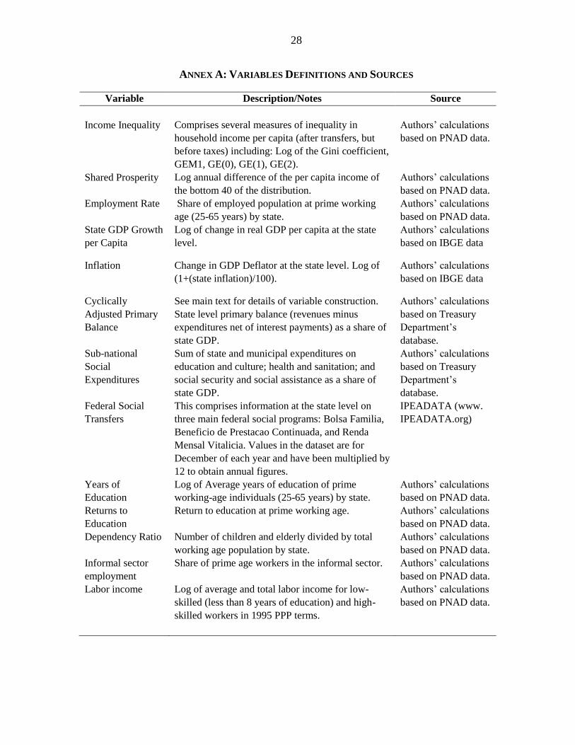
ANNEX A: VARIABLES DEFINITIONS AND SOURCES
Variable Description/Notes Source
Income Inequality Comprises several measures of inequality in
household income per capita (after transfers, but
before taxes) including: Log of the Gini coefficient,
GEM1, GE(0), GE(1), GE(2).
Authors’ calculations
based on PNAD data.
Shared Prosperity Log annual difference of the per capita income of
the bottom 40 of the distribution.
Authors’ calculations
based on PNAD data.
Employment Rate Share of employed population at prime working
age (25-65 years) by state.
Authors’ calculations
based on PNAD data.
State GDP Growth
per Capita
Log of change in real GDP per capita at the state
level.
Authors’ calculations
based on IBGE data
Inflation Change in GDP Deflator at the state level. Log of
(1+(state inflation)/100).
Authors’ calculations
based on IBGE data
Cyclically
Adjusted Primary
Balance
See main text for details of variable construction.
State level primary balance (revenues minus
expenditures net of interest payments) as a share of
state GDP.
Authors’ calculations
based on Treasury
Department’s
database.
Sub-national
Social
Expenditures
Sum of state and municipal expenditures on
education and culture; health and sanitation; and
social security and social assistance as a share of
state GDP.
Authors’ calculations
based on Treasury
Department’s
database.
Federal Social
Transfers
This comprises information at the state level on
three main federal social programs: Bolsa Familia,
Beneficio de Prestacao Continuada, and Renda
Mensal Vitalicia. Values in the dataset are for
December of each year and have been multiplied by
12 to obtain annual figures.
IPEADATA (www.
IPEADATA.org)
Years of
Education
Log of Average years of education of prime
working-age individuals (25-65 years) by state.
Authors’ calculations
based on PNAD data.
Returns to
Education
Return to education at prime working age. Authors’ calculations
based on PNAD data.
Dependency Ratio Number of children and elderly divided by total
working age population by state.
Authors’ calculations
based on PNAD data.
Informal sector
employment
Share of prime age workers in the informal sector. Authors’ calculations
based on PNAD data.
Labor income Log of average and total labor income for low-
skilled (less than 8 years of education) and high-
skilled workers in 1995 PPP terms.
Authors’ calculations
based on PNAD data.
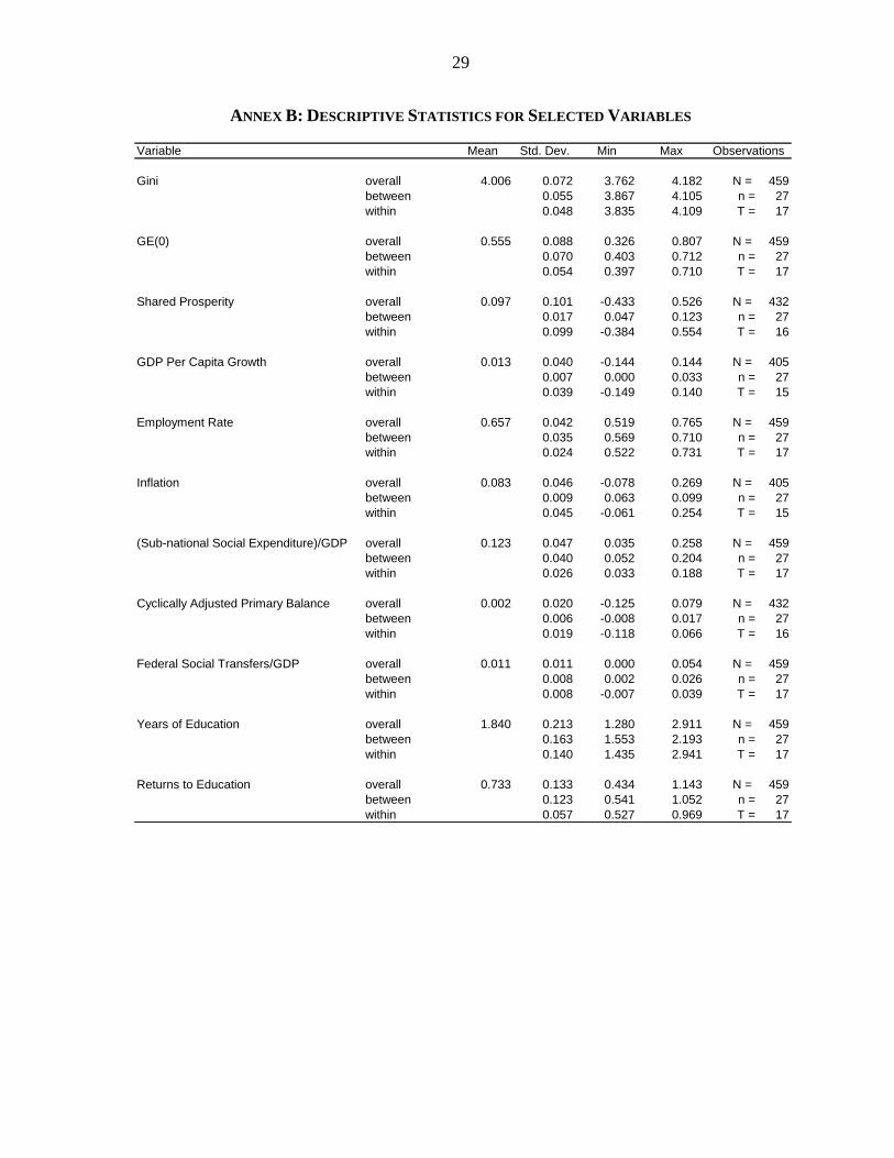
29
ANNEX B: DESCRIPTIVE STATISTICS FOR SELECTED VARIABLES
Variable Mean Std. Dev. Min Max Observations
Gini overall 4.006 0.072 3.762 4.182 N = 459
between 0.055 3.867 4.105 n = 27
within 0.048 3.835 4.109 T = 17
GE(0) overall 0.555 0.088 0.326 0.807 N = 459
between 0.070 0.403 0.712 n = 27
within 0.054 0.397 0.710 T = 17
Shared Prosperity overall 0.097 0.101 -0.433 0.526 N = 432
between 0.017 0.047 0.123 n = 27
within 0.099 -0.384 0.554 T = 16
GDP Per Capita Growth overall 0.013 0.040 -0.144 0.144 N = 405
between 0.007 0.000 0.033 n = 27
within 0.039 -0.149 0.140 T = 15
Employment Rate overall 0.657 0.042 0.519 0.765 N = 459
between 0.035 0.569 0.710 n = 27
within 0.024 0.522 0.731 T = 17
Inflation overall 0.083 0.046 -0.078 0.269 N = 405
between 0.009 0.063 0.099 n = 27
within 0.045 -0.061 0.254 T = 15
(Sub-national Social Expenditure)/GDP overall 0.123 0.047 0.035 0.258 N = 459
between 0.040 0.052 0.204 n = 27
within 0.026 0.033 0.188 T = 17
Cyclically Adjusted Primary Balance overall 0.002 0.020 -0.125 0.079 N = 432
between 0.006 -0.008 0.017 n = 27
within 0.019 -0.118 0.066 T = 16
Federal Social Transfers/GDP overall 0.011 0.011 0.000 0.054 N = 459
between 0.008 0.002 0.026 n = 27
within 0.008 -0.007 0.039 T = 17
Years of Education overall 1.840 0.213 1.280 2.911 N = 459
between 0.163 1.553 2.193 n = 27
within 0.140 1.435 2.941 T = 17
Returns to Education overall 0.733 0.133 0.434 1.143 N = 459
between 0.123 0.541 1.052 n = 27
within 0.057 0.527 0.969 T = 17
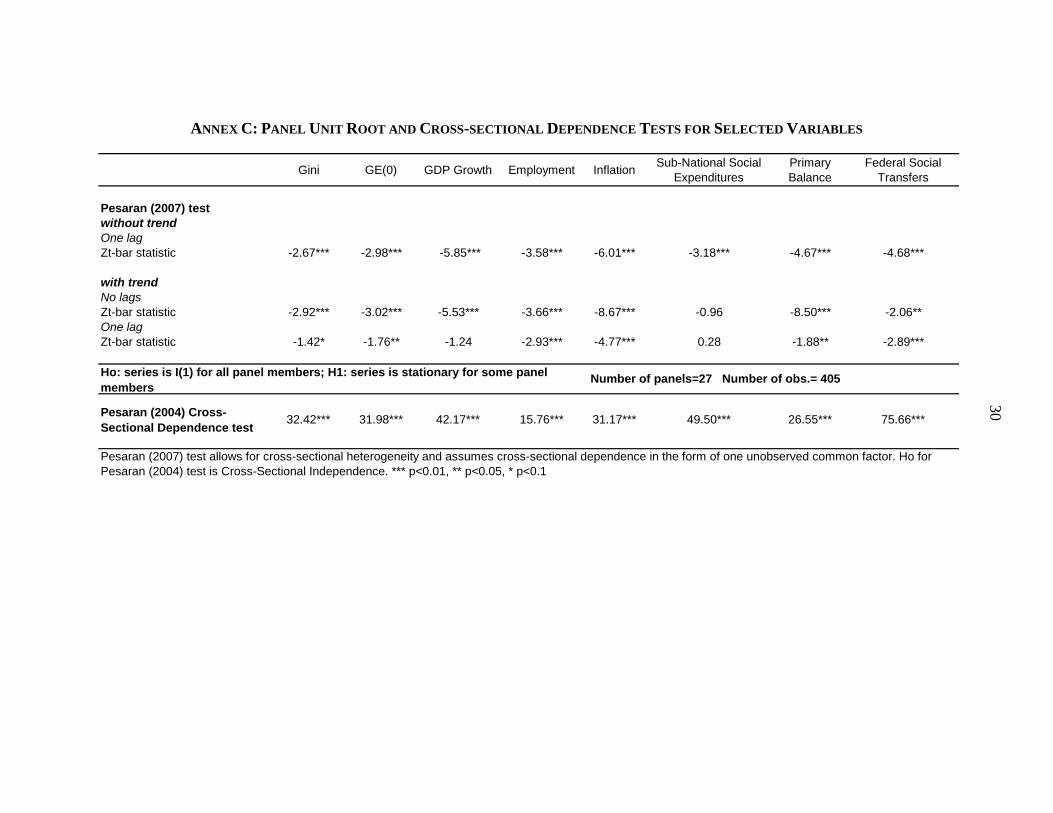
30
ANNEX C: PANEL UNIT ROOT AND CROSS-SECTIONAL DEPENDENCE TESTS FOR SELECTED VARIABLES
Gini GE(0) GDP Growth Employment InflationSub-National Social
Expenditures
Primary
Balance
Federal Social
Transfers
Pesaran (2007) test
without trend
One lag
Zt-bar statistic -2.67*** -2.98*** -5.85*** -3.58*** -6.01*** -3.18*** -4.67*** -4.68***
with trend
No lags
Zt-bar statistic -2.92*** -3.02*** -5.53*** -3.66*** -8.67*** -0.96 -8.50*** -2.06**
One lag
Zt-bar statistic -1.42* -1.76** -1.24 -2.93*** -4.77*** 0.28 -1.88** -2.89***
75.66***
Pesaran (2007) test allows for cross-sectional heterogeneity and assumes cross-sectional dependence in the form of one unobserved common factor. Ho for
Pesaran (2004) test is Cross-Sectional Independence. *** p<0.01, ** p<0.05, * p<0.1
Number of panels=27 Number of obs.= 405Ho: series is I(1) for all panel members; H1: series is stationary for some panel
members
Pesaran (2004) Cross-
Sectional Dependence test32.42*** 26.55***31.98*** 42.17*** 15.76*** 31.17*** 49.50***